Numerical piecewise approximate solution of Fredholm integro-differential equations by the Tau method

www.elsevier.com/locate/apm

Applied Mathematical Modelling 29 (2005) 1005–1021

Numerical piecewise approximate solution of Fredholmintegro-differential equations by the Tau method

S. Mohammad Hosseini a,*, S. Shahmorad b

a Department of Mathematics, Tarbiat Modarres University, P.O. Box 14115-175, Tehran, Iranb Department of Applied Mathematics, Tabriz University, Tabriz, Iran

Received 1 October 2003; received in revised form 1 December 2004; accepted 8 February 2005Available online 19 March 2005

Abstract

A general form of numerical piecewise approximate solution of linear integro-differential equations ofFredholm type is discussed. It is formulated for using the operational Tau method to convert the differentialpart of a given integro-differential equation, or IDE for short, to its matrix representation. This formulationof the Tau method can be useful for such problems over long intervals and also can be used as a good andsimple alternative algorithm for other piecewise approximations such as splines or collocation. A Tau errorestimator is also adapted for piecewise application of the Tau method. Some numerical examples are con-sidered to demonstrate the implementation and general effect of application of this (segmented) piecewiseChebyshev Tau method.� 2005 Elsevier Inc. All rights reserved.

Keywords: Piecewise approximate; Piecewise Tau method; Integro-differential equations; Segmented Tau method

1. Introduction

We extend (see [1–4]), the operational approach of the Tau method (see [5]), to the numericalsolution of general form of linear Fredholm and Volterra integro-differential equations and obtainaccurate results, except for the problems defined over a long interval.

0307-904X/$ - see front matter � 2005 Elsevier Inc. All rights reserved.doi:10.1016/j.apm.2005.02.003

* Corresponding author.E-mail address: [email protected] (S.M. Hosseini).

1006 S.M. Hosseini, S. Shahmorad / Applied Mathematical Modelling 29 (2005) 1005–1021

In this method, we only replace the operator matrix representation for the differential part ofthe equation using the operational Tau method. However, a full matrix formulation of the Taumethod [3] can also be implemented, for which the details appear in another paper. The remainderof the paper is organized as follows:

Section 2, is devoted to introducing the problem and some preliminary results concerning theTau method. In Section 3, details of the formulation of the new method are explained. In Section4, the way of implementing the method is demonstrated. Section 5 provides some numericalresults used to clarify the efficiency of the method.

2. The problem and some preliminary results of the Tau method

Let us consider the general linear Fredholm integro-differential equation

DyðxÞ � kZ b

akðx; tÞyðtÞdt ¼ f ðxÞ; x 2 ½a; b� ð2:1Þ

with m independent conditions

cð1Þjk yðk�1ÞðaÞ þ cð2Þjk y

ðk�1ÞðbÞh i

¼ cj; j ¼ 1; . . . ; m; ð2:2Þ

where cj is constant and m is the order of the differential operator D with polynomial coefficientspi(x)

D ¼Xmr¼0

prðxÞdr

dxr; prðxÞ ¼

Xarj¼0

prjxj ¼ p

rX ; ð2:3Þ

where ar is the degree of pr(x), pr¼ ðpr0; pr1; . . . ; prar ; 0; 0; . . .Þ and X ¼ ð1; x; . . . ÞT.

k(x,t) is a bivariate polynomial or its bivariate Tau polynomial approximation of degree pairs,say, (k1,k2). Similarly, f(x) is a polynomial or a suitable polynomial approximation of it.

The operational Tau method is generally based on three simple matrices

g ¼

0 0 0 0 � � �1 0 0 0 � � �0 2 0 0 � � �... ..

. ... ..

. . ..

0BBBB@

1CCCCA; l ¼

0 1 0 0 � � �0 0 1 0 � � �0 0 0 1 � � �... ..

. ... ..

. . ..

0BBBB@

1CCCCA; i ¼

0 1 0 0 � � �0 0 1

20 � � �

0 0 0 13

� � �

..

. ... ..

. ... . .

.

0BBBB@

1CCCCA:

In this paper, we have only used g, l for the differential part of (2.1). See [5] for more applica-tion of these three matrices. The matrices g, l have the following effects:

Lemma 2.1. If yn(x) = anX, with an = (a0,a1, . . . , an, 0,0, . . .), then

dynðxÞdx

¼ angX ; xynðxÞ ¼ a

nlX :

Let V = {vi(x):i = 0,1, . . .} be a polynomial base given by V = VX where V is a nonsingular lowertriangular matrix and V �1 its inverse.

S.M. Hosseini, S. Shahmorad / Applied Mathematical Modelling 29 (2005) 1005–1021 1007

We recall the following theorem from [5]:

Theorem 2.2. For any linear differential operator D defined by (2.3) and any series y(x) = bV, b =(b0,b1, . . .) or y(x) = aX, a = (a0,a1, . . .) we have

DyðxÞ ¼ aYx

X ¼ bYv

V ; ð2:4Þ

where

¼Xmi¼0

gipiðlÞ;Yv

¼ VYx

V �1: ð2:5Þ

3. Formulation of the piecewise method

Let

a ¼ x0 < x1 < � � � < xn ¼ b

be a partition of [a,b], and

½xi�m; xðiþ1Þ�m�;

m, be subintervals of [a,b], on which we want to approximate the solu-tion y(x) of (2.1) and (2.2), as pieces of polynomials yi(x) of degree m with unknown coefficientsyi0, . . .,yim, i.e.,

yðxÞ �

Pmj¼0

y0jv�0jðxÞ; x 2 ½x0; xm�;

Pmj¼0

y1jv�1jðxÞ; x 2 ½xm; x2m�;

..

. ...

Pmj¼0

yp�1;jv�p�1jðxÞ; x 2 ½xn�m; xn�;

8>>>>>>>>>>><>>>>>>>>>>>:

ð3:1Þ

where the basis functions v�ijðxÞ are shifted to suitable polynomials (such as Chebyshev or Legen-dre) of degree j in [xi·m,x(i+1)·m] for j = 0,1, . . .. We set

V �i ¼ v�i0ðxÞ; v�i1ðxÞ; . . .

� �T ð3:2Þ

so that expansion of the functions k(x,t), f(x) and y(x) for x 2 [xi·m, x(i+1)·m], t 2 [tj·m, t(j+1)·m]and i, j = 0,1, . . ., p � 1, can be expressed as

kðx; tÞ �Xmr¼0

Xmq¼0

kijrqv�irðxÞv�jqðtÞ; ð3:3Þ

f ðxÞ � fiðxÞ ¼Xmr¼0

firv�irðxÞ ¼ fiV �

i ð3:4Þ

1008 S.M. Hosseini, S. Shahmorad / Applied Mathematical Modelling 29 (2005) 1005–1021

and

yðxÞ � yiðxÞ ¼Xmr¼0

yirv�irðxÞ ¼ y

iV �

i ; ð3:5Þ

where fi = (fi0, fi1, . . ., fim, 0,0, . . .) and yi = (yi0,yi1, . . ., yim, 0,0, . . .).Hence, on [xi·m,x(i+1)·m], using Theorem 2.2, we have

DyðxÞ ¼ yi

Yvi

V �i : ð3:6ÞQ

Note that viis computed by (2.5), after restricting V to this subinterval.

Substituting k(x,t) and yi(t) from (3.3) and (3.5) into integral part of (2.1), one obtains

akðx; tÞyiðtÞdt �

Xmr¼0

Xmq¼0

Xml¼0

Xp�1

j¼0

yjlkijrqv�irðxÞ

Z tðjþ1Þ�m

tj�m

v�jqðtÞv�jlðtÞdt: ð3:7Þ

Setting

aljq ¼Z tðjþ1Þ�m

tj�m

v�jqðtÞv�jlðtÞdt ð3:8Þ

the coefficient of v�irðxÞ in (3.7) is then as follows:

Xmq¼0

Xml¼0

Xp�1

j¼0

yjlkijrqaljq ¼Xp�1

j¼0

yjRðiÞjr ð3:9Þ

with

RðiÞjr ¼

Pmq¼0

kijrqa0jq

..

.

Pmq¼0

kijrqamjq

0BBBBBB@

1CCCCCCA; i; j ¼ 0; 1; . . . ; p � 1: ð3:10Þ

So that

Z b

akðx; tÞyiðtÞdt �

Xmr¼0

Xp�1

j¼0

yjRðiÞjr

!v�irðxÞ ¼

Xp�1

j¼0

yjRðiÞj0 ; . . . ;R

ðiÞjm

� �V �

i

¼Xp�1

j¼0

yjAij

!V �

i ; i ¼ 0; 1; . . . ; p � 1 ð3:11Þ

with

Aij ¼ RðiÞj0 ; . . . ;R

ðiÞjm

� �: ð3:12Þ

S.M. Hosseini, S. Shahmorad / Applied Mathematical Modelling 29 (2005) 1005–1021 1009

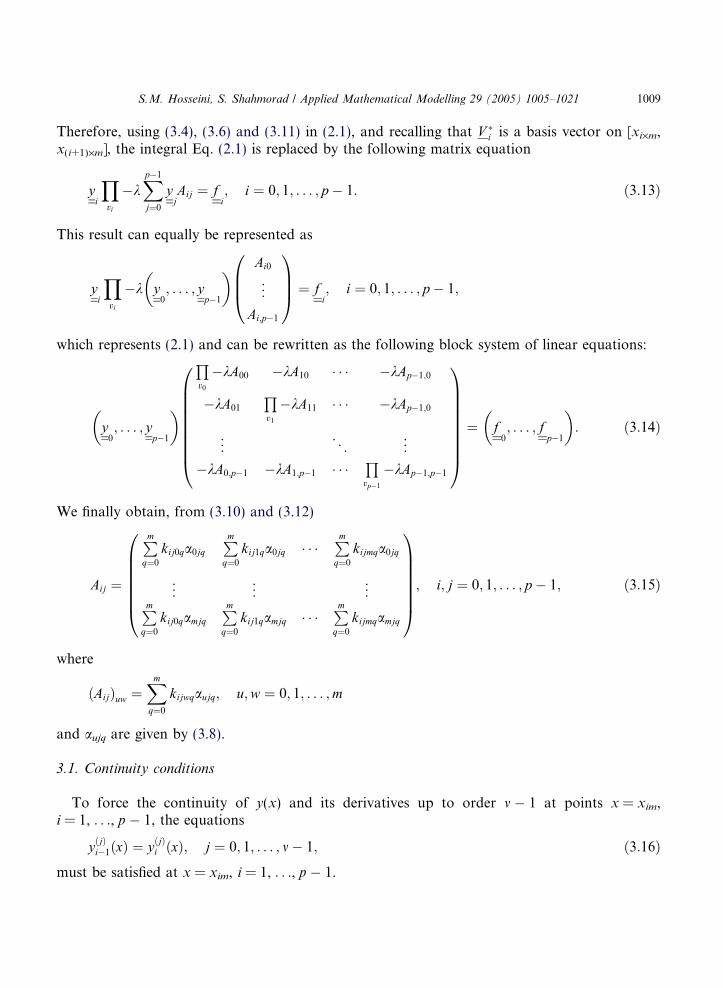
Therefore, using (3.4), (3.6) and (3.11) in (2.1), and recalling that V �i is a basis vector on [xi·m,

x(i+1)·m], the integral Eq. (2.1) is replaced by the following matrix equation

yi

Yvi

�kXp�1

j¼0

yjAij ¼ f

i; i ¼ 0; 1; . . . ; p � 1: ð3:13Þ

This result can equally be represented as

yi

Yvi

�k y0; . . . ; y

p�1

� � Ai0

..

.

Ai;p�1

0BB@

1CCA ¼ f

i; i ¼ 0; 1; . . . ; p � 1;

which represents (2.1) and can be rewritten as the following block system of linear equations:

y0; . . . ; y

p�1

� �Qv0

�kA00 �kA10 � � � �kAp�1;0

�kA01

Qv1

�kA11 � � � �kAp�1;0

..

. . .. ..

.

�kA0;p�1 �kA1;p�1 � � �Qvp�1

�kAp�1;p�1

0BBBBBBBB@

1CCCCCCCCA

¼ f0; . . . ; f

p�1

� �: ð3:14Þ

We finally obtain, from (3.10) and (3.12)

Aij ¼

Pmq¼0

kij0qa0jqPmq¼0

kij1qa0jq � � �Pmq¼0

kijmqa0jq

..

. ... ..

.

Pmq¼0

kij0qamjqPmq¼0

kij1qamjq � � �Pmq¼0

kijmqamjq

0BBBBBB@

1CCCCCCA; i; j ¼ 0; 1; . . . ; p � 1; ð3:15Þ

where

ðAijÞuw ¼Xmq¼0

kijwqaujq; u;w ¼ 0; 1; . . . ;m

and aujq are given by (3.8).

3.1. Continuity conditions

To force the continuity of y(x) and its derivatives up to order m � 1 at points x = xim,i = 1, . . ., p � 1, the equations

yðjÞi�1ðxÞ ¼ yðjÞi ðxÞ; j ¼ 0; 1; . . . ; m� 1; ð3:16Þ

1010 S.M. Hosseini, S. Shahmorad / Applied Mathematical Modelling 29 (2005) 1005–1021

Satisfying (3.16) at x = xim, from (3.5) and since degree of v�ij 6 j , one obtains

yi�1

v�i�1;0ðximÞ 0 � � � 0

v�i�1;1ðximÞ v�ð1Þi�1;1ðximÞ � � � 0

..

. ... ..

.

v�i�1;m�1ðximÞ v�ð1Þi�1;m�1ðximÞ � � � v�ðm�1Þi�1;m�1ðximÞ

..

. ... ..

.

v�i�1;mðximÞ v�ð1Þi�1;mðximÞ � � � v�ðm�1Þi�1;m ðximÞ

0BBBBBBBBBBBBB@

1CCCCCCCCCCCCCA

� yi

v�i;0ðximÞ 0 � � � 0

v�i;1ðximÞ v�ð1Þi;1 ðximÞ � � � 0

..

. ... ..

.

v�i;m�1ðximÞ v�ð1Þi;m�1ðximÞ � � � v�ðm�1Þi;m�1 ðximÞ

..

. ... ..

.

v�i;mðximÞ v�ð1Þi;m ðximÞ � � � v�ðm�1Þi;m ðximÞ

0BBBBBBBBBBBBB@

1CCCCCCCCCCCCCA

¼ ð0; 0; . . . ; 0Þ: ð3:17Þ

3.2. Matrix representation for supplementary conditions

Since a 2 [x0,xm] and b 2 [xn � m,xn], the supplementary conditions (2.2) must be written as

Xmk¼1

cð1Þjk yðk�1ÞðaÞ þ cð2Þjk y

ðk�1ÞðbÞ� �

¼Xmk¼1

cð1Þjk yðk�1Þ0 ðaÞ þ cð2Þjk y

ðk�1Þp�1 ðbÞ

� �

¼Xmk¼1

cð1Þjk yðk�1Þ0 ðaÞ þ

Xmk¼1

cð2Þjk yðk�1Þp�1 ðbÞ ð3:18Þ

and since

yiðxÞ ¼Xmr¼0

yirv�irðxÞ; i ¼ 0; 1; . . . ; p � 1;

we have for the first term of (3.18)

Xmk¼1

cð1Þjk yðk�1Þ0 ðaÞ ¼

Xmk¼1

cð1Þjk

Xmr¼0

y0rv�0rðaÞ

!¼Xmr¼0

y0rXmk¼1

cð1Þjk v�0rðaÞ ¼ y

0B0j

with

S.M. Hosseini, S. Shahmorad / Applied Mathematical Modelling 29 (2005) 1005–1021 1011

B0j ¼

cð1Þj1 v�00ðaÞP2

k¼1

cð1Þjk v�ðk�1Þ01 ðaÞ

..

.

Pmk¼1

cð1Þjk v�ðk�1Þ0;m�1 ðaÞ

..

.

Pmk¼1

cð1Þjk v�ðk�1Þ0m ðaÞ

0BBBBBBBBBBBBBBBBB@

1CCCCCCCCCCCCCCCCCA

: ð3:19Þ

Similarly, for the second term of (3.18)

Xmk¼1

cð2Þjk yðk�1Þp�1 ðbÞ ¼

Xmk¼1

cð2Þjk

Xmr¼0

yp�1;rv�p�1;rðbÞ

!¼Xmr¼0

yp�1;r

Xmk¼1

cð2Þjk v�p�1;rðbÞ ¼ y

p�1Bp�1;j

with

Bp�1;j ¼

cð2Þj1 v�p�1;0ðbÞP2

k¼1

cð2Þjk v�ðk�1Þp�1;1 ðbÞ

..

.

Pmk¼1

cð2Þjk v�ðk�1Þp�1;m�1ðbÞ

..

.

Pmk¼1

cð2Þjk v�ðk�1Þp�1;m ðbÞ

0BBBBBBBBBBBBBBBBB@

1CCCCCCCCCCCCCCCCCA

: ð3:20Þ

Hence

Xmk¼1

cð1Þjk yðk�1ÞðaÞ þ cð2Þjk y

ðk�1ÞðbÞ� �

¼ y0B0j þ y

p�1Bp�1;j; j ¼ 1; . . . ; m: ð3:21Þ

We refer to B as the supplementary conditions matrix, B0j and Bp�1,j as jth columns of the sub-matrices of B in the first and last subintervals.

3.3. Determining the final linear equations

We recall that we want to approximate y(x) with

yiðxÞ ¼Xmr¼0

yirv�irðxÞ ¼ y

iV �

i

1012 S.M. Hosseini, S. Shahmorad / Applied Mathematical Modelling 29 (2005) 1005–1021

in each subinterval of the form [xi·m,x(i+1)·m]. Since there are p subintervals of this form, the num-ber of required unknowns and corresponding linear equations will be (m + 1) · p. Note that thenumber of equations that can be obtained from continuity conditions (3.17) is equal to (p � 1) · m.We also obtain m equations from supplementary conditions (3.21). So, the total number of equa-tions that can be obtained from the continuity and supplementary conditions will be p · m. There-fore, we need

ðmþ 1Þ � p � p � m ¼ ðmþ 1� mÞ � p;

other linear equations that must be obtained from (3.14).Therefore, we have the following three steps:

Step 1. For i,j = 0, . . ., p � 1, l1 = 0, . . ., m and l2 = 0, . . ., m � m, set

ðGijÞl1;l2 ¼Qvj

�kAij

!l1;l2

; if i ¼ j;

�kðAjiÞl1;l2 ; if i 6¼ j;

8>><>>:

ðFjÞl2 ¼ ðf

jÞl2 :

Step 2. For i = 0, . . ., p � 1, l1 = 0, . . ., m and l2 = m � m + 1 . . .,m, set

ðGi�1;i�1Þl1;l2 ¼ ðCi�1Þl1;l2 ;

ðGi;i�1Þl1;l2 ¼ ðCiÞl1;l2 ;

ðFi�1

Þl2 ¼ 0;

where Ci�1 and Ci are matrices corresponding to continuity conditions.Step 3. For l1 = 0, . . ., m and l2 = 1, . . ., m, set

ðGi;p�1Þl1;m�mþl2¼

ðBil2Þl1 ; for i ¼ 0; p � 1;

0; for i ¼ 1; . . . ; p � 2;

�

ðFp�1

Þm�mþl2¼ cl2 :

By these three steps, we make the block system

y0; . . . ; y

p�1

� � G00 G10 � � � G0;p�1

G10 G11 � � � G1;p�1

..

. . .. ..

.

Gp�1;0 Gp�1;1 � � � Gp�1;p�1

0BBBB@

1CCCCA ¼ F

0; . . . ; F

p�1

� �ð3:22Þ

and solve it for the vectors

y0; . . . ; y

p�1

S.M. Hosseini, S. Shahmorad / Applied Mathematical Modelling 29 (2005) 1005–1021 1013

by a Gaussian elimination method in which, to avoid direct inversion of diagonal blocks, we haveapplied the QR factorization, providing the possibility of taking advantage of numerical stabilityof QR method.

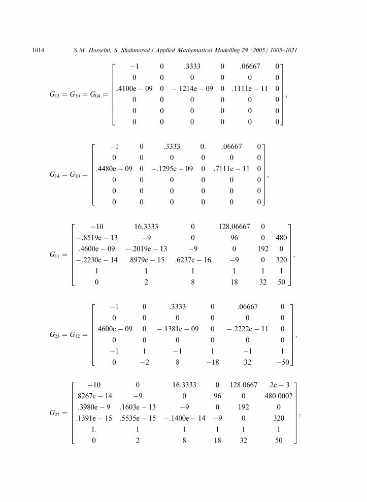
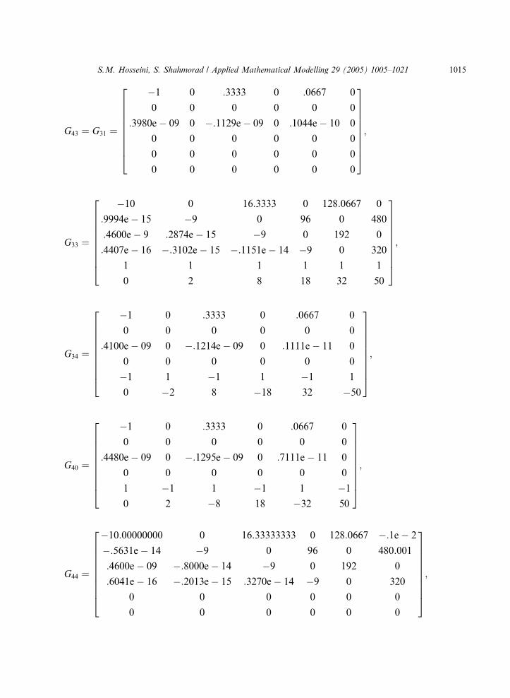
4. How to implement this piecewise method

To show the structure of final system (3.22), we give block matrices Gij and other related vectorsfor

y00ðxÞ ¼ 9yðxÞ þ e�15 � 1

3þZ 5

0

yðtÞdt; x 2 ½0; 5�

yð0Þ ¼ 1;

y0ð0Þ ¼ �3

with exact solution y(x) = e�3x for m = 5, p = 5

G00 ¼

�10 0 16:3333 0 128:0667 0

0 �9 0 96 0 480

:4600e� 9 :7674e� 14 �9 0 192 0

0 :7780e� 14 :2185e� 14 �9 0 320

1 1 1 1 1 1

0 2 8 18 32 50

2666666664

3777777775;

G01 ¼

�1 0 :3333 0 :0667 0

0 0 0 0 0 0

:3980e� 09 0 �:1129e� 09 0 :1044e� 10 0

0 0 0 0 0 0

�1 1 �1 1 �1 1

0 �2 8 �18 32 �50

2666666664

3777777775;

G03 ¼ G20 ¼ G21 ¼ G24 ¼ G32 ¼ G41 ¼ G42 ¼ G02

¼

�1 0 :3333 0 :06667 0

0 0 0 0 0 0

:4600e� 09 0 �:1381e� 09 0 �:2222e� 11 0

0 0 0 0 0 0

0 0 0 0 0 0

0 0 0 0 0 0

26666666664

37777777775;

1014 S.M. Hosseini, S. Shahmorad / Applied Mathematical Modelling 29 (2005) 1005–1021

G13 ¼ G30 ¼ G04 ¼

�1 0 :3333 0 :06667 0

0 0 0 0 0 0

:4100e� 09 0 �:1214e� 09 0 :1111e� 11 0

0 0 0 0 0 0

0 0 0 0 0 0

0 0 0 0 0 0

2666666664

3777777775;

G14 ¼ G10 ¼

�1 0 :3333 0: :06667 0

0 0 0 0 0 0

:4480e� 09 0 �:1295e� 09 0 :7111e� 11 0

0 0 0 0 0 0

0 0 0 0 0 0

0 0 0 0 0 0

2666666664

3777777775;

G11 ¼

�10 16:3333 0 128:06667 0

�:8519e� 13 �9 0 96 0 480

:4600e� 09 �:2019e� 13 �9 0 192 0

�:2230e� 14 :8979e� 15 :6237e� 16 �9 0 320

1 1 1 1 1 1

0 2 8 18 32 50

2666666664

3777777775;

G23 ¼ G12 ¼

�1 0 :3333 0 :06667 0

0 0 0 0 0 0

:4600e� 09 0 �:1381e� 09 0 �:2222e� 11 0

0 0 0 0 0 0

�1 1 �1 1 �1 1

0 �2 8 �18 32 �50

2666666664

3777777775;

G22 ¼

�10 0 16:3333 0 128:0667 :2e� 3

:8267e� 14 �9 0 96 0 480:0002

:3980e� 9 :1603e� 13 �9 0 192 0

:1391e� 15 :5535e� 15 �:1400e� 14 �9 0 320

1: 1 1 1 1 1

0 2 8 18 32 50

2666666664

3777777775;

S.M. Hosseini, S. Shahmorad / Applied Mathematical Modelling 29 (2005) 1005–1021 1015

G43 ¼ G31 ¼

�1 0 :3333 0 :0667 0

0 0 0 0 0 0

:3980e� 09 0 �:1129e� 09 0 :1044e� 10 0

0 0 0 0 0 0

0 0 0 0 0 0

0 0 0 0 0 0

2666666664

3777777775;

G33 ¼

�10 0 16:3333 0 128:0667 0

:9994e� 15 �9 0 96 0 480

:4600e� 9 :2874e� 15 �9 0 192 0

:4407e� 16 �:3102e� 15 �:1151e� 14 �9 0 320

1 1 1 1 1 1

0 2 8 18 32 50

2666666664

3777777775;

G34 ¼

�1 0 :3333 0 :0667 0

0 0 0 0 0 0

:4100e� 09 0 �:1214e� 09 0 :1111e� 11 0

0 0 0 0 0 0

�1 1 �1 1 �1 1

0 �2 8 �18 32 �50

2666666664

3777777775;

G40 ¼

�1 0 :3333 0 :0667 0

0 0 0 0 0 0

:4480e� 09 0 �:1295e� 09 0 :7111e� 11 0

0 0 0 0 0 0

1 �1 1 �1 1 �1

0 2 �8 18 �32 50

2666666664

3777777775;

G44 ¼

�10:00000000 0 16:33333333 0 128:0667 �:1e� 2

�:5631e� 14 �9 0 96 0 480:001

:4600e� 09 �:8000e� 14 �9 0 192 0

:6041e� 16 �:2013e� 15 :3270e� 14 �9 0 320

0 0 0 0 0 0

0 0 0 0 0 0

2666666664

3777777775;

Table 1Maximum absolute error

m p

1 2 3 4 5

3 1.61e+00 8.79e+00 2.15e�01 6.34e�01 1.59e+005 2.1e+00 8.31e�01 1.63e�01 4.71e�02 4.40e�0210 1.56e�02 1.50e�04 3.81e�06 2.66e�07 8.26e�08

1016 S.M. Hosseini, S. Shahmorad / Applied Mathematical Modelling 29 (2005) 1005–1021

F0¼ F

1¼ F

2¼ F

3¼ F

4¼ �:3333 0 0 0 0 0½ �:

Then the coefficient vector solutions y0,y1,y2,y3,y4, on the subintervals [0.0,1.0], [1.0,2.0], [2.0,3.0],[3.0,4.0], [4.0,5.0], respectively, are

y0¼ :3680 �:4378 :1501 �:3599e� 1 :7036e� 2 �:1012e� 2½ �;

y1¼ :1920e� 1 �:2159e� 1 :7402e� 2 �:1775e� 2 :34696e� 3 �:4992e� 4½ �;

y2¼ :1961e� 2 �:1113e� 2 :3486e� 3 �:9147e� 4 :1634e� 4 �:2572e� 5½ �;

y3¼ :3357e� 3 �:1027e� 2 �:3163e� 3 �:8445e� 4 �:1483e� 4 �:2375e� 5½ �;

y4¼ �:1546e� 1 �:1977e� 1 �:6778e� 2 �:1625e� 2 �:31770e� 3 �:4571e� 4½ �:

See Table 1 for further numerical results of this example.

5. Error estimation

When the solution is not known, the need for an error estimator presents itself as a vital com-ponent for any given algorithm. To this end, one can follow the same lines of a similar discussionin [1] and extend the method for piecewise approximation. Let us call em(x) = y(x) � ym(x) the‘‘mth-order Tau error function’’ which is to be approximated by the same method of Tau.For an integro-differential equation ID(y) = 0 with conditions B(y) = b0, the Tau problemID(ym) = Hm(x) with B(ym(x)) = b0 is associated which is defined by the same integro-differentialoperator ID; Hm(x) is a polynomial of degree m chosen for the exact solution ym(x) to be a poly-nomial of a prescribed degree. Subtracting the equations related to the Tau problem from those ofthe exact problem one obtains the Tau error problem ID(em(x)) = �Hm(x), with B(em(x)) = 0.

Like the original problem we proceed in the same manner to estimate em(x) with the Taumethod. We seek a polynomial approximation em,n(x) for n > m which provides the Tau errorestimation and is denoted by ‘‘Est.Err’’ in the following Table 6. The terms ‘‘exact’’, ‘‘Tau’’,and ‘‘Ext.Err’’ denote exact solution, Tau approximate solution, and difference between thosevalues, respectively.

S.M. Hosseini, S. Shahmorad / Applied Mathematical Modelling 29 (2005) 1005–1021 1017

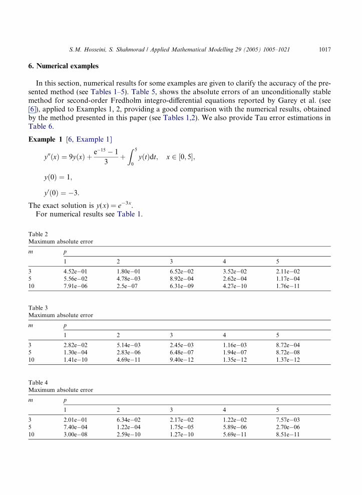
6. Numerical examples

In this section, numerical results for some examples are given to clarify the accuracy of the pre-sented method (see Tables 1–5). Table 5, shows the absolute errors of an unconditionally stablemethod for second-order Fredholm integro-differential equations reported by Garey et al. (see[6]), applied to Examples 1, 2, providing a good comparison with the numerical results, obtainedby the method presented in this paper (see Tables 1,2). We also provide Tau error estimations inTable 6.

Example 1 [6, Example 1]

TableMaxim

m

3510

TableMaxim

m

3510

TableMaxim

m

3510

y00ðxÞ ¼ 9yðxÞ þ e�15 � 1

3þZ 5

0

yðtÞdt; x 2 ½0; 5�;

yð0Þ ¼ 1;

y0ð0Þ ¼ �3:

The exact solution is y(x) = e�3x.For numerical results see Table 1.

2um absolute error

p

1 2 3 4 5

4.52e�01 1.80e�01 6.52e�02 3.52e�02 2.11e�025.56e�02 4.78e�03 8.92e�04 2.62e�04 1.17e�047.91e�06 2.5e�07 6.31e�09 4.27e�10 1.76e�11

3um absolute error

p

1 2 3 4 5

2.82e�02 5.14e�03 2.45e�03 1.16e�03 8.72e�041.30e�04 2.83e�06 6.48e�07 1.94e�07 8.72e�081.41e�10 4.69e�11 9.40e�12 1.35e�12 1.37e�12

4um absolute error

p

1 2 3 4 5

2.01e�01 6.34e�02 2.17e�02 1.22e�02 7.57e�037.40e�04 1.22e�04 1.75e�05 5.89e�06 2.70e�063.00e�08 2.59e�10 1.27e�10 5.69e�11 8.51e�11

Table 5Summary of errors (en = yn � y(xn), h = .10)

(L = 0.0) (L = 5.0)

xn yn en yn en

Example 11.0 .04917 �6.167(�4) .04981 2.274(�5)2.0 .00079 �1.679(�3) .00248 2.632(�6)3.0 �.00442 �4.540(�3) .00012 �1.955(�6)4.0 �.01239 �1.240(�2) �.00004 �4.346(�5)5.0 �.03626 �3.624(�2) �.00087 �8.740(�4)

Example 21.0 .13522 �1.086(�4) .13535 1.922(�5)2.0 .01809 �2.241(�4) .01832 �3.111(�7)3.0 .00204 �4.390(�4) .00248 �3.718(�6)4.0 �.00532 �8.672(�4) .00033 �2.863(�6)5.0 �.00174 �1.787(�3) .00004 3.346(�6)

Note. In [6] L is a nonnegative parameter and is referred to as a stabilization parameter.

1018 S.M. Hosseini, S. Shahmorad / Applied Mathematical Modelling 29 (2005) 1005–1021

Example 2 [6, Example 2]

y 00ðxÞ ¼ 4yðxÞ þ 1

2ln

xþ e�10

xþ 1

� �þZ 5

0

yðtÞxþ e�2x

dt; x 2 ½0; 5�;

yð0Þ ¼ 1;

y 0ð0Þ ¼ �2:

The exact solution is yðxÞ ¼ e�2x.For numerical results see Table 2.

Example 3 [7, p. 136]

y 00ðxÞ ¼ yðxÞ � 4

p

Z p2

0

xtyðtÞdt; x 2 0;p2

h i;

yð0Þ ¼ 0;

y 0ð0Þ ¼ 1:

The exact solution is yðxÞ ¼ sinðxÞ.For numerical results see Table 3.

Example 4 [8, p. 361]

y 00ðxÞ ¼ yðxÞ � 4

p

Z p

0

cosðx� tÞyðtÞdt; x 2 ½0;p�;

yð0Þ ¼ 1;

y 0ðpÞ ¼ 0:

Table 6The error-estimation ‘‘Est.err’’ for Example 4, (m = 5, n = 7)

s Exact Tau Ext.err Est.err

[0.00, 0.79]0.00 1.00000000 1.00000000 2.600e�09 5.300e�140.10 0.99500417 0.99500529 1.125e�06 1.129e�060.20 0.98006658 0.98006793 1.350e�06 1.352e�060.30 0.95533649 0.95533756 1.076e�06 1.079e�060.40 0.92106099 0.92106237 1.381e�06 1.385e�060.50 0.87758256 0.87758525 2.688e�06 2.691e�060.60 0.82533561 0.82534001 4.400e�06 4.403e�060 .70 0.76484219 0.76484764 5.449e�06 5.453e�06

[0.79, 1.57]0.79 0.70710678 0.70711245 5.664e�06 5.668e�060.89 0.63298131 0.63298726 5.950e�06 5.954e�060.99 0.55253129 0.55253710 5.807e�06 5.810e�061.09 0.46656057 0.46656601 5.441e�06 5.444e�061.19 0.37592812 0.37593343 5.308e�06 5.311e�061.29 0.28153953 0.28154508 5.548e�06 5.551e�061.39 0.18433789 0.18434377 5.885e�06 5.887e�061.49 0.08529440 0.08530030 5.896e�06 5.898e�06

[1.57, 2.36]1.57 �0.00000000 0.00000561 5.612e�06 5.612e�061.67 �0.09983342 �0.09982817 5.243e�06 5.242e�061.77 �0.19866933 �0.19866418 5.152e�06 5.151e�061.87 �0.29552021 �0.29551498 5.224e�06 5.223e�061.97 �0.38941834 �0.38941331 5.035e�06 5.033e�062.07 �0.47942554 �0.47942118 4.361e�06 4.359e�062.17 �0.56464247 �0.56463906 3.411e�06 3.408e�062.27 �0.64421769 �0.64421503 2.657e�06 2.653e�06

[2.36, 3.14]2.36 �0.70710678 �0.70710451 2.274e�06 2.267e�062.46 �0.77416708 �0.77416533 1.744e�06 1.739e�062.56 �0.83349215 �0.83349012 2.036e�06 2.029e�062.66 �0.88448925 �0.88448646 2.791e�06 2.785e�062.76 �0.92664883 �0.92664587 2.951e�06 2.953e�062.86 �0.95954963 �0.95954757 2.061e�06 2.058e�062.96 �0.98286293 �0.98286223 6.990e�07 6.860e�073.06 �0.99635579 �0.99635583 3.730e�08 4.700e�08

S.M. Hosseini, S. Shahmorad / Applied Mathematical Modelling 29 (2005) 1005–1021 1019

The exact solution is yðxÞ ¼ cosðxÞ.For numerical results see Table 4.

6.1. Examples for the Tau estimator

To clarify the efficiency and use of the Tau estimator, we consider again the test Example 4. Thenumerical results for (m = 5,n = 7) are given in Table 6. The results confirm that Ext.err andEst.err are in good agreement.

1020 S.M. Hosseini, S. Shahmorad / Applied Mathematical Modelling 29 (2005) 1005–1021

Example 5. We consider a test problem in which the coefficients are not polynomial and againconfirms that the Tau method is capable of dealing with such problems without having to facevery much computational effort. Again, well agreement between exact and estimated errors isillustrated in Table 7.

TableThe e

s

[�1.0�1.�0.�0.�0.�0.�0.

[�0.5�0.�0.�0.�0.�0.0.00

[0.00,0.000.100.200.300.400.50

[0.50,0.500.600.700.800.901.00

exy 00ðxÞ þ cosðxÞy 0ðxÞ þ sinðxÞyðxÞ þZ 1

�1

eððxþ1ÞtÞyðtÞdt

¼ ðcosðxÞ þ sinðxÞ þ exÞex þ 2sinhðxþ 2Þ

xþ 2; x 2 ½�1; 1�;

yð�1Þ þ yð1Þ ¼ eþ 1=e;

yð�1Þ � y0ð�1Þ þ yð1Þ ¼ e:

The exact solution is y(x) = exp(x).

7rror-estimation ‘‘Est.err’’ for Example 5, (m = 9, n = 11)

Exact Tau Ext.err Est.err

0,�0.50]00 0.36787944 0.36787792 1.521e�06 1.748e�0690 0.40656966 0.40656806 1.604e�06 1.826e�0680 0.44932896 0.44932722 1.746e�06 1.958e�0670 0.49658530 0.49658343 1.871e�06 2.072e�0660 0.54881164 0.54880968 1.958e�06 2.148e�0650 0.60653066 0.60652865 2.008e�06 2.188e�06

0,0.00]50 0.60653066 0.60652865 2.008e�06 2.188e�0640 0.67032005 0.67031802 2.025e�06 2.193e�0630 0.74081822 0.74081621 2.012e�06 2.170e�0620 0.81873075 0.81872878 1.975e�06 2.122e�0610 0.90483742 0.90483550 1.917e�06 2.052e�06

1.00000000 0.99999816 1.839e�06 1.963e�06

0.50]1.00000000 0.99999816 1.839e�06 1.963e�061.10517092 1.10516917 1.744e�06 1.855e�061.22140276 1.22140113 1.632e�06 1.732e�061.34985881 1.34985730 1.506e�06 1.593e�061.49182470 1.49182333 1.367e�06 1.440e�061.64872127 1.64872006 1.215e�06 1.275e�06

1.00]1.64872127 1.64872006 1.215e�06 1.275e�061.82211880 1.82211775 1.047e�06 1.094e�062.01375271 2.01375186 8.493e�07 8.807e�072.22554093 2.22554037 5.562e�07 5.648e�072.45960311 2.45960315 4.018e�08 8.766e�082.71828183 2.71828335 1.522e�06 1.748e�06

S.M. Hosseini, S. Shahmorad / Applied Mathematical Modelling 29 (2005) 1005–1021 1021

7. Conclusions

The formulation of the piecewise Tau method, or segmented Tau, was given. We demonstratedthe implementation and accuracy of the method for some examples with different degrees and seg-mentations. Although in the classical Tau method one is required to use an initial approximation ofthe nonpolynomial coefficient functions appearing in the equation, this should not cause anyone tohesitate about applying the Taumethod and taking advantage of its features that have already beenintroduced through different papers during last 30 years. However, in some examples that we haveconsidered, the coefficients and the kernels are nonpolynomials which have been replaced by easilyobtained interpolating polynomials based on zeros of the Chebyshev polynomials. Comparisonswith some other well known methods have often been reported in some related articles, but herewe would particularly like to comment on the application of the classical collocation method. In[9] it has been shown that collocation approximations of any given degree can be simulated throughthe Tau method by using a special perturbation term. In doing so, the collocation method acquiresthe permanence property of the Taumethod and consequently the number of arithmetic operationsrequired to compute collocation approximations can be reduced considerably.

We finally have adapted a Tau estimator to estimate the error of approximations on each seg-ment. The results given in Tables 6 and 7 confirm the efficiency of the introduced Tau errorestimator.

References

[1] S.M. Hosseini, S. Shahmorad, Numerical solution of a class of integro-differential equations with the Tau methodwith an error estimation, Appl. Math. Comput. 136 (2003) 559–570.

[2] S.M. Hosseini, S. Shahmorad, Tau numerical solution of Fredholm integro-differential equations with arbitrarypolynomial bases, Appl. Math. Model 27 (2003) 145–154.

[3] S.M. Hosseini, S. Shahmorad, A matrix formulation of the tau for the Fredholm and Volterra linear integro-differential equations, Korean J. Comput. Appl. Math. 9 (2) (2002) 497–507.

[4] S. Shahmorad, Numerical solution of a class of integro-differential equations by the Tau method, Ph.D Thesis,Tarbiat Modarres University, Tehran, 2002.

[5] E.L. Ortiz, H. Samara, An operational approach to the Tau method for the numerical solution of nonlineardifferential equations, Computing 27 (1981) 15–25.

[6] L.E. Garey, C.J. Gladwin, R.E. Shaw, Unconditionally stable method for second-order Fredholm integro-differential equations, Appl. Math. Comput. 81 (1997) 275–286.

[7] A.M. Wazwaz, A First Course in Integral Equations, World Scientific, River Edge, NJ, 1997.[8] L.M. Delves, J.L. Mohamed, Computational Methods for Integral Equations, Cambridge University Press,

Cambridge, 1985.[9] M.K. EL-Daou, E.L. Ortiz, A recursive formulation of collocation in terms of canonical polynomials, Computing

52 (1994) 177–202.