• • •

Welcome message from author
This document is posted to help you gain knowledge. Please leave a comment to let me know what you think about it! Share it to your friends and learn new things together.
Transcript
Durham E-Theses
Numerical modelling of the stress regime at subduction
zones
Waghorn, G. D.
How to cite:
Waghorn, G. D. (1984) Numerical modelling of the stress regime at subduction zones, Durham theses,Durham University. Available at Durham E-Theses Online: http://etheses.dur.ac.uk/7581/
Use policy
The full-text may be used and/or reproduced, and given to third parties in any format or medium, without prior permission orcharge, for personal research or study, educational, or not-for-pro�t purposes provided that:
• a full bibliographic reference is made to the original source
• a link is made to the metadata record in Durham E-Theses
• the full-text is not changed in any way
The full-text must not be sold in any format or medium without the formal permission of the copyright holders.
Please consult the full Durham E-Theses policy for further details.
Academic Support O�ce, Durham University, University O�ce, Old Elvet, Durham DH1 3HPe-mail: [email protected] Tel: +44 0191 334 6107
http://etheses.dur.ac.uk
NUMERICAL MODELLING OF THE
STRESS REGIME
AT SUBDUCT ION ZONES
by
G.D. WAGHORN
The copyright of this thesis rests with the author.
No quotation from it should be published without
his prior written consent and information derived
from it should be acknowledged.
A t h e s i s s u b m i t t e d t o t h e U n i v e r s i t y
o f Durham f o r t h e Degree o f
Doctor o f P h i l o s o p h y
Graduate S o c i e t y November 1984
ABSTRACT
The s t r e s s regime a t s u b d u c t i o n zones has been m o d e l l e d u s i n g a
v i s c o - e l a s t i c , q u a d r a t i c i s o p a r a m e t r i c f i n i t e element model. An
i s o p a r a m e t r i c model i s used because i t p e r f o r m s more a c c u r a t e l y t h a n
c o n s t a n t s t r a i n t r i a n g u l a r elements (CST) and a l s o a l l o w s c u r v e d s i d e d
elements t o be i n t r o d u c e d .
A method f o r m o d e l l i n g t h e f r i c t i o n a l s l i d i n g on i s o p a r a m e t r i c f a u l t
e lements has been d e v e l o p e d by e x t e n d i n g M i t h e n ' s (1980) CST model. The
r e s u l t i n g method i s s u i t a b l e f o r m o d e l l i n g t h e d e f o r m a t i o n on b o t h p l a n e
and l i s t r i c , normal and t h r u s t f a u l t s . Graben w i d t h s p r e d i c t e d by normal
f a u l t models agree w i t h a n a l y t i c s o l u t i o n s and t h i s i m p l i e s t h a t M i t h e n ' s
CST models f a i l e d t o do so because t h e y were to o s t i f f .
A p p l i c a t i o n o f t h i s modal t o s u b d u c t i o n zones d e m o n s t r a t e s t h a t t h e
s l a b p u l l f o r c e i n d u c e s t e n s i o n i n t h e s u b d u c t i n g p l a t e and c o m p r e s s i o n i n
t h e o v e r l y i n g p l a t e . P a r t o f t h e l a t e r a l v a r i a t i o n i n s t r e s s w h i c h i s
o b s e r v e d a t a l l s u b d u c t i o n zones i s t h e r e f o r e i n f e r r e d t o a r i s e f r o m t h e
s l a b p u l l f o r c e . D i f f e r e n c e s i n t h e magnitude o f t h e s e s t r e s s e s a t
d i f f e r e n t s u b d u c t i o n zones may t h e r e f o r e be a c c o u n t e d f o r by l o c a l
v a r i a t i o n s i n t h e magnitude o r d i p o f t h e s l a b p u l l f o r c e , and a l s o by t h e
e x t e n t o f t h e c o u p l i n g a c r o s s t h e p l a t e boundary.
V a r i o u s f o r c e s a c c o u n t f o r t h e s t r e s s regime i n back a r c r e g i o n s .
T e n s i o n a l s t r e s s i s g e n e r a t e d by l a t e r a l d e n s i t y v a r i a t i o n s , and t h e
h e a t i n g and s h e a r i n g caused by s l a b i n d u c e d c o n v e c t i o n . Compressive
s t r e s s , a r i s i n g f r o m t h e s l a b p u l l f o r c e , i s superimposed upon t h i s . The
magnitude o f t h e c o m p r e s s i o n , however, i s dependent upon t h e d i p and s i z e
o f t h e s l a b p u l l f o r c e and a l s o t h e degree o f m e c h a n i c a l c o u p l i n g between
t h e p l a t e s a t t h e s u b d u c t i o n zone f a u l t . L o c a l v a r i a t i o n s i n t h e m a g n i t u d e
of t h e c ompressive s t r e s s may t h e r e f o r e e x p l a i n why t h e s t r e s s regime i s
o b s erved t o be so v a r i a b l e i n back a r c r e g i o n s , and i s more commonly
t e n s i o n than c o m p r e s s i o n .
ACKNOWLEDGEMENTS
I would l i k e t o express my g r a t i t u d e t o my s u p e r v i s o r , P r o f . M.H.P.
B o t t , f o r h i s h e l p f u l c r i t i c i s m s d u r i n g t h e 3 ye a r s o f my r e s e a r c h , and t o
Dr. M.D. L i n t o n f o r many i l l u m i n a t i n g d i s c u s s i o n s about f i n i t e element
t e c h n i q u e s . I would a l s o l i k e t o thank M.J. Snuth f o r f o r w a r d i n g some
f i n a l p l o t s t o me i n London.
T h i s r e s e a r c h was done w h i l s t I was i n r e c e i p t o f a s t u d e n t s h i p f r o m
NERC, t o whom I am v e r y g r a t e f u l .
F i n a l l y , I would l i k e t o express my g r a t i t u d e t o B.P. f o r p r o v i d i n g
t h e s u p p o r t and f a c i l i t i e s t o complete t h i s t h e s i s .
" On t h e f i r s t day t h e y had gone up t o t h e
mountains and had a p i c n i c i n t h e p i n e f o r e s t .
'We g o t a c o u r s e i n p i c n i c k i n g a t t h i s u n i v e r s i t y , '
s a i d Dr. Bourbon.
' I t ' s c a l l e d g e o l o g y , b u t i t ' s r e a l l y p i c n i c k i n g ' "
M. B r a d b u r y
CONTENTS
Page
ABSTRACT
ACKNOWLEDGEMENTS
CONTENTS
CHAPTER 1 AN INTRODUCTION TO SU2DUCTI0N ZONES
1.1 Ev i d e n c e For S u b d u c t i o n 2
1.1.1 S e i s m o l o g i c a l e v i d e n c e 3
1.1.2 Other g e o p h y s i c a l e v i d e n c e 4
1.2 Morphology And Deep S t r u c t u r e Of "Subduction Zones . 6
1.3 Thermal S t r u c t u r e Of S u b d u c t i o n Zones. 9
1.3.1 Thermal s t r u c t u r e o f t h e s u b d u c t i n g p l a t e . . . . 9
1.3.2 The t h e r m a l regime o f t h e o v e r l y i n g p l a t e and t h e
a s t h e n o s p h e r i c wedge 10
1.4 The Observed S t a t e Of S t r e s s At S u b d u c t i o n Zones . 11
1.4.1 T r e n c h - o u t e r r i s e system 12
1.4.2 The l e a d i n g edge o f t h e o v e r l y i n g p l a t e . . . . 13
1.4.3 S u b d u c t i n g p l a t e 15
1.4.4 Back a r c r e g i o n s 16
1.5 Sources Of S t r e s s 21
1.6 Aims Of The T h e s i s 24
CHAPTER 2 THE RHEOLOGY OF THE LITHOSPHERE
2.1 I n t r o d u c t i o n 25
2.2 R h e o l o g i c a l Response Of The E a r t h To P e r s i s t e n t
G e o l o g i c a l Loads 26
2.3 S e i s m o l o g i c a l Evidence 27
2.3.1 Seismic e v i d e n c e f o r t h e l i t h o s p h e r e and
as t h e n o s p h e r e 27
2.3.2 V a r i a t i o n o f e l a s t i c p a r a m e t e r s w i t h d e p t h . . . 28
2.3.3 N o n - e l a s t i c d e f o r m a t i o n 28
2.4 L i t h o s p h e r i c F l e x u r e 29
2.5 Rock Mechanics 30
2.5.1 B r i t t l e f r a c t u r e : m o d i f i e d G r i f f i t h t h e o r y . . . 31
2.5.2 D u c t i l e b e h a v i o u r 34
2.6 C o n c l u s i o n : A R h e o l o g i c a l Model Of The L i t h o s p h e r e 37
CHAPTER 3 THE ISOPARAMETRIC FINITE ELEMENT METHOD
3.1 I n t r o d u c t i o n 39
3.2 The L o c a l C o - o r d i n a t e System 41
3.2.1 L o c a l c o - o r d i n a t e system f o r t r i a n g u l a r elements 41
3.2.2 L o c a l c o - o r d i n a t e system f o r q u a d r i l a t e r a l
elements 42
3.3 The I s o p a r a m e t r i c Concept 42
3.4 Shape F u n c t i o n s 43
3.4.1 G e n e r a l d e f i n i t i o n and e v a l u a t i o n o f shape
f u n c t i o n s 44
3.4.2 Shape f u n c t i o n s o f a t r i a n g u l a r element . . . . 46
3.4.3 D i s p l a c e m e n t shape f u n c t i o n s 46
3.4.3.1 Geometric shape f u n c t i o n s 49
3.4.4 Shape f u n c t i o n s f o r q u a d r i l a t e r a l elements . . . 49
3.4.4.1 D i s p l a c e m e n t shape f u n c t i o n s 49
3.4.4.2 Geometric shape f u n c t i o n s 52
3.4.5 Summary 52
3.5 D i f f e r e n t i a t i o n And I n t e g r a t i o n Of The Shape
F u n c t i o n s 54
3.5.1 D i f f e r e n t i a t i o n : The J a c o b i a n m a t r i x 54
3.5.2 I n t e g r a t i o n : N u m e r i c a l i n t e g r a t i o n 55
3.6 E v a l u a t i o n Of The S t i f f n e s s M a t r i x 57
3.6.1 The s t r a i n m a t r i x 57
3.6.2 The e l a s t i c i t y m a t r i x 60
3.6.3 The s t i f f n e s s m a t r i x 61
3.7 Nodal R e p r e s e n t a t i o n Of Forces 64
3.7.1 Body f o r c e s 65
3.7.2 S u r f a c e t r a c t i o n 65
3.7.2.1 The l o c a l c o - o r d i n a t e system 65
3.7.2.2 Nodal r e p r e s e n t a t i o n o f f o r c e s due t o a s u r f a c e
t r a c t i o n 67
3.7.2.3 I s o s t a t i c c o m p e n s a t i o n 69
3.8 Thermal S t r e s s e s 70
3.9 V i s c o - e l a s t i c A n a l y s i s 70
CHAPTER 4 COMPARISON OF FINITE ELEMENTS
4.1 I n t r o d u c t i o n 73
4.2 C o n s t a n t S t r a i n Elements 73
4.3 C a n t i l e v e r Bending 75
4.3.1 A n a l y t i c s o l u t i o n 75
4.3.2 F i n i t e element s o l u t i o n s 75
4.4 Body Forces 78
4.4.1 A n a l y t i c s o l u t i o n 78
4.4.2 F i n i t e e i nent s o l u t i o n s 79
4.5 V i s c o - e l a s t i c C y l i n d e r 82
4.5.1 A n a l y t i c s o l u t i o n 82
4.5.2 F i n i t e element s o l u t i o n s 83
4.6 Summary Ana C o n c l u s i o n s 35
CHAPTER 5 THE ISOPARAMETRIC FINITE ELEMENT FAULT MODEL
5.1 I n t r o d u c t i o n 87
5.2 Review Of F i n i t e Element F a u l t Models 88
5.3 L o c a l C o - o r d i n a t e System For A F a u l t Element . . . 90
5.4 S t i f f n e s s Of An I s o p a r a m e t r i c F a u l t Element . . . 91
5.5 M o d e l l i n g Of F r i c t i o n a l S l i d i n g 95
5.5.1 C a l c u l a t i o n o f t h e s t r e s s on t h e f a u l t p l a n e . . 95
5.5.2 S l i p c o n d i t i o n s 98
5.5.3 C a l c u l a t i o n o f t h e excess shear s t r e s s and f a u l t
f o r c e v e c t o r 98
5.5.4 I t e r a t i o n t o remove t h e excess shear s t r e s s . . 99
CHAPTER 6 FRICTIONAL SLIDING ON PLANE AND LISTRIC FAULTS
6.1 F r i c t i o n a l S l i d i n g On A Plane S i d e d Normal F a u l t . 100
6.1.1 D e s c r i p t i o n o f t h e f i n i t e element mesh 100
6.1.2 Response o f t h e f i n i t e element model t o f l e x u r e 101
6.1.3 I n i t i a l e l a s t i c d e f o r m a t i o n o f t h e model . . . . 102
6.1.4 F r i c t i o n a l s l i d i n g i n response t o a 50 MPa
t e n s i o n 105
6.1.5 Convergence f a c t o r 106
6.1.6 F r i c t i o n a l s l i d i n g i n response t o 40 and 30 MPa
t e n s i o n 107
6.1.7 P r e d i c t e d g r a ben w i d t h s 108
6.1.3 I s o s t a t i c c o mpensation on t h e upper s u r f a c e o f
t h e model I l l
6.2 L i s t r i c Normal F a u l t 112
6.2.1 D e s c r i p t i o n o f t h e f i n i t e element mesh 112
6.2.2 D i s c u s s i o n o f r e s u l t s 113
6.3 T h r u s t F a u l t s 114
6.3.1 Plane t h r u s t f a u l t s 114
6.3.2 L i s t r i c t h r u s t f a u l t s . . .- 115
6.4 Summary And C o n c l u s i o n s 117
CHAPTER 7 THE STRESS -REGIME AT SUBDUCTION ZONES
7.1 I n t r o d u c t i o n 119
7.2 D e s c r i p t i o n Of The F i n i t e Element Mesh 119
7.3 L a t e r a l D e n s i t y V a r i a t i o n s 122
7.3.1 D e s c r i p t i o n o f t h e f i n i t e element model 123
7.3.2 D i s c u s s i o n o f r e s u l t s 124
7.3.3 F u r t h e r c o n s i d e r a t i o n s : Other l a t e r a l d e n s i t y
v a r i a t i o n s a t s u b d u c t i o n zones 126
7.3.4 L i m i t a t i o n s o f t h e models 127
7.4 Slab P u l l 129
7.4.1 D e s c r i p t i o n o f t h e f i n i t e element model . . . . 130
7.4.2 The s t r e s s regime produced by a v e r t i c a l s l a b
p u l l f o r c e 132
7.4.3 E f f e c t o f a d i p p i n g s l a b p u l l f o r c e 134
7.4.4 D i s c u s s i o n 135
7.4.5 L i m i t a t i o n s o f t h e models 136
7.5 E f f e c t Of The S u b d u c t i o n Zone F a u l t 136
7.5.1 D e s c r i p t i o n o f t h e f i n i t e element model . . . . 137
7.5.2 E f f e c t o f r e d u c i n g t h e shear s t i f f n e s s o f t h e
s u b d u c t i o n zone f a u l t 138
7.5.3 D i s c u s s i o n 140
7.6 C o n v e c t i o n I n The A s t h e n o s p h e r i c Wedge 141
7.6.1 E f f e c t o f shear s t r e s s 142
7.6.2 E f f e c t o f t h e r m a l volume changes 144
7.6.3 D i s c u s s i o n 146
7.7 Summary And C o n c l u s i o n s 148
CHAPTER 8 SUMMARY AND CONCLUSIONS «, 153
APPENDIX A COMPUTER PROGRAMS
A . l I n t r o d u c t i o n 158
A.2 ISOLIB: D e s c r i p t i o n Of S u b r o u t i n e s 159
A.2.1 F i n i t e element s u b r o u t i n e s 159
A.2.2 E x t e r n a l s u b r o u t i n e s 161
A.3 ISOFELP: The C o n s t r u c t i o n Of A C a l l i n g Sequence . 161
A.4 U t i l i s a t i o n 161
A.4.1 I n p u t s p e c i f i c a t i o n : Device 4 162
A.4.2 I n p u t s p e c i f i c a t i o n : Device 3 169
A.4.3 I n p u t s p e c i f i c a t i o n : Device 5 170
A. 4.4 Running t h e programs 170
A.5 Program L i s t i n g s 172
FERENCES 224
CHAPTER 1
AN INTRODUCTION TO SUBDUCTION ZONES
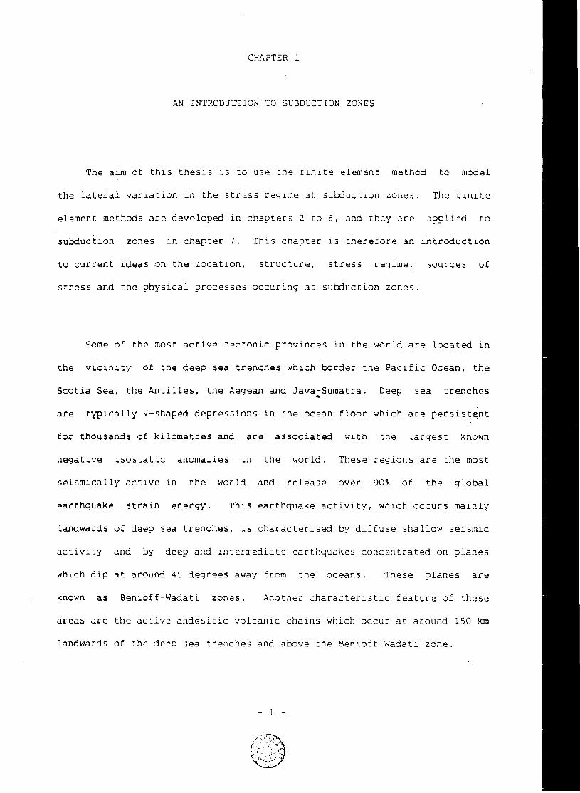
The aim o f t h i s t h e s i s i s t o use t h e f i n i t e element method t o model
th e l a t e r a l v a r i a t i o n i n t h e s t r 3 s s regime a t s u b d u c t i o n zones. The f i n i t e
element methods a r e d e v e l o p e d i n c h a p t e r s 2 t o 6, and t h e y a r e a p p l i e d t o
s u b d u c t i o n zones i n c h a p t e r 7. T h i s c h a p t e r i s t h e r e f o r e an i n t r o d u c t i o n
t o c u r r e n t i d e a s on t h e l o c a t i o n , s t r u c t u r e , s t r e s s r e g i m e , sources o f
s t r e s s and t h e p h y s i c a l p r o c e s s e s o c c u r i n g a t s u b d u c t i o n zones.
Some o f t h e most a c t i v e t e c t o n i c p r o v i n c e s i n t h e w o r l d a r e l o c a t e d i n
t h e v i c i n i t y o f th e deep sea t r e n c h e s w h i c h b o r d e r t h e P a c i f i c Ocean, t h e
S c o t i a Sea, t h e A n t i l l e s , t h e Aegean and Java-Sumatra. Deeo sea t r e n c h e s
a r e t y p i c a l l y v-shaped d e p r e s s i o n s i n t h e ocean f l o o r w h i c h a r e p e r s i s t e n t
f o r thousands o f k i l o m e t r e s and a r e a s s o c i a t e d w i t h t h e l a r g e s t known
n e g a t i v e i s o s t a t i c a n o m a l i e s i n t h e w o r l d . These r e g i o n s a r e t h e most
s e i s m i c a l l y a c t i v e i n t h e w o r l d and r e l e a s e over 90% o f t h e g l o b a l
e a r t h q u a k e s t r a i n e n ergy. T h i s e a r t h q u a k e a c t i v i t y , w h i c h o c c u r s m a i n l y
landwards o f deep sea t r e n c h e s , i s c h a r a c t e r i s e d by d i f f u s e s h a l l o w s e i s m i c
a c t i v i t y and by deep and i n t e r m e d i a t e e a r t h q u a k e s c o n c e n t r a t e d on p l a n e s
which d i p a t around 45 degrees away fr o m t h e oceans. These p l a n e s a r e
known as B e n i o f f - W a d a t i zones. Another c h a r a c t e r i s t i c f e a t u r e o f t h e s e
areas a r e t h e a c t i v e a n d e s i t i c v o l c a n i c c h a i n s which o c c u r a t aro u n d 150 km
landwards o f the deep sea t r e n c h e s and above t h e S e n i o f f - W a d a t i zone.
- 1 -
D u r i n g t h e l a s t t w e n t y y e a r s i t has been r e a l i s e d t h a t t h e t e c t o n i c
a c t i v i t y w h i c h o c c u r s a t deep sea t r e n c h e s o r i g i n a t e s f r o m a common cause,
t h e s u b d u c t i o n o f o c e a n i c l i t h o s p h e r e . I n t h e s u b d u c t i o n h y p o t h e s i s deep
sea t r e n c h e s a r e c o n s i d e r e d t o be t h e s i t e s a t which two l i t h o s p h e r i c
p l a t e s a r e c o n v e r g i n g w i t h t h e r e s u l t t h a t an o c e a n i c p l a t e i s t h r u s t
beneath t h e o t h e r p l a t e and r e c y c l e d i n t o t h e m a n t l e . T h i s c o n c e p t forms
an i n t e g r a l p a r t o f t h e t h e o r y o f p l a t e t e c t o n i c s .
The e v i d e n c e w h i c h s u p p o r t s t h e h y p o t h e s i s t h a t s u b d u c t i o n o c c u r s a t
deep sea t r e n c h e s i s d i s c u s s e d i n t h e n e x t s e c t i o n .
1.1 Evidence For S u b d u c t i o n
The concep t t h a t t h e o c e a n i c l i t h o s p h e r e i s b e i n g s u b d u c t e d a r i s e s
f r o m two i m p o r t a n t g e o p h y s i c a l o b s e r v a t i o n s . The f i r s t o f t h e s e i s t h a t
new r i g i d p l a t e s o f o c e a n i c l i t h o s p h e r e a r e b e i n g c r e a t e d a t mid ocean
r i d g e s by t h e p r o c e s s o f sea f l o o r s p r e a d i n g ( V i n e and Matthews, 1963).
The second p i e c e o f e v i d e n c e , which has r e c e n t l y been r e v i e w e d by B o t t
( 1 9 8 2 a ) , i s t h a t t h e e a r t h i s p r o b a b l y n o t expanding by any s i g n i f i c a n t
amount. The l o g i c a l consequence o f these two o b s e r v a t i o n s i s t h a t o c e a n i c
l i t h o s p h e r e must be c o n t i n u o u s l y r e c y c l e d ( i . e . s u bducted) back i n t o t h e
m a n t l e somewhere.
T h i s p r o c e s s i s p r o b a b l y o c c u r i n g a t deep sea t r e n c h e s . The
o b s e r v a t i o n s w h i c h s u p p o r t t h i s h y p o t h e s i s a re m a i n l y s e i s m o l o g i c a l b u t
o t h e r g e o p h y s i c a l e v i d e n c e has been i m p o r t a n t i n d e m o n s t r a t i n g t h e
f e a s i b i l i t y o f t h i s c o n c e p t .
- 2 -
1.1.1 S e i s m o l o g i c a l e v i d e n c e
The most c o n v i n c i n g e v i d e n c e which s u p p o r t s t h e h y p o t h e s i s t h a t
s u b d u c t i o n o c c u r s a t deep sea t r e n c h e s i s based on t h e f o l l o w i n g
s e i s m o l o g i c a l o b s e r v a t i o n s ( I s a c k s e t a l , 1968):
1. Almost a l l deep and i n t e r m e d i a t e e a r t h q u a k e s a r e s p a t i a l l y
c o n r e n t r a t e d a t deep sea t r e n c h e s .
2. The h y p o c e n t r e s o f t h e s e e a r t h q u a k e s f a l l on a p l a n e w h i c h d i p s a t
30-80 degrees away f r o m t h e t r e n c h and to w a r d s t h e v o l c a n i c a r c
( B e n i o f f , 1954; Sykes, 1966; I s a c k s and B a r a z a n g i , 1977). T h i s
p l a n e i s known as t h e B e n o i f f - W a d a t i zone.
3. The B e n i o f f - W a d a t i zone i n t e r s e c t s t h e e a r t h % s u r f a c e c l o s e t o t h e
a x i s o f deep sea t r e n c h e s (Sykes, 1966).
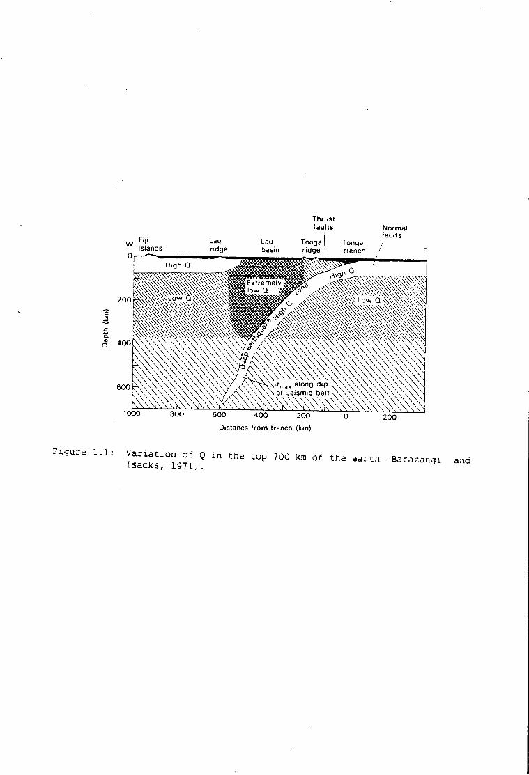
4. The 3 e n i o f f - W a d a t i zone i s l o c a t e d i n t h e upper 30 km o f an
anomalous r e g i o n o f h i g h Q i n an o t h e r w i s e low Q upper m a n t l e
( O l i v e r and I s a c k s , 1 9 6 7 ) . T h i s tongue o f h i g h Q i s a p p r o x i m a t e l y
100 km t h i c k and i s c o n t i n u o u s w i t h , and has s i m i l a r p r o p e r t i e s
t o , t h e o c e a n i c l i t h o s p h e r e ( F i g u r e 1 . 1 ) . T h i s f e a t u r e was
i n i t i a l l y o b s e r v e d i n t h e t h e F i j i - T o n g a r e g i o n b u t i t has
s u b s e q u e n t l y been o b s e r v e d a t o t h e r s u b d u c t i o n zones ( e . g . U t s u ,
1971).
Recent i n v e s t i g a t i o n s have d e m o n s t r a t e d t h a t a r e g i o n o f
e x t r e m e l y low Q o c c u r s i m m e d i a t e l y above t h e h i g h Q ton g u e
( B a r a z a n g i and I s a c k s , 1971).
5. A d d i t i o n a l e v i d e n c e , w h i c h was r e v i e w e d by I s a c k s e t a l ( 1 9 6 8 ) ,
comes f r o m t h e f o c a l mechanism s o l u t i o n s o f t h e e a r t h q u a k e s i n
- 3 -
Thrust faults Normal
faults Lau basin
Tonga / trench / Islands
Extremely
m „ along dip of seismic belt
600 400 200
Distance from trench (km) 200
F i g u r e 1.1: V a r i a t i o n o f Q i n t h e t o p 700 km o f t h e e a r t h ( B a r a z a n g i and I s a c k s , 1 9 7 1 ) .
s u b d u c t i o n zones. The s h a l l o w e a r t h q u a k e s have two t y p e s o f f o c a l
mechanisms. These a r e t e n s i o n a l i n t h e s u b d u c t i n g p l a t e and
c o m p r e s s i v e i n t h e o v e r l y i n g p l a t e . T h i s s u g g e s t s t h a t
u n d e r t h r u s t i n g i s o c c u r i n g i n t h e s e r e g i o n s .
I n t e r m e d i a t e and deep e a r t h q u a k e s have t h e i r axes o f maximum
and minimum p r i n c i p a l s t r e s s a J i g n e d down t h e d i o o f t h e
B e n i o f f - W a d a t i zone and i n t e r m e d i a t e p r i n c i p a l s t r e s s p a r a l l e l and
h o r i z o n t a l t o t h e s t r i k e o f t h e B e n i o f f Zone. These o b s e r v a t i o n s
a r e c o n s i s t e n t w i t h t h e r e l e a s e o f s t r e s s which would o c c u r w i t h i n
a s i n k i n g p l a t e o f o c e a n i c l i t h o s p h e r e <;isacks and M o l n a r , 1969).
Double p l a n e d B e n i o f f - W a d a t i zones have been o b s e r v e d between
100 and 150 km d e p t h a t some, b u t n o t a l l , s u b d u c t i o n zones
( F u j i t a and Kanamori, 1981). The e a r t h q u a k e s on t h e upper p l a n e
a r e l o c a t e d near t o t h e t o p o f t h e s u b d u c t i n g p l a t e and have
c o m p r e s s i v e f o c a l mechanisms. About 30 km beneath t h i s a l o w e r
p l a n e o f e a r t h q u a k e s w i t h t e n s i o n a l f o c a l mechanisms i s o b s e r v e d .
T h i s s t r e s s regime may be caused e i t h e r by t h e r m a l s t r e s s
(Woodward, 1975), an unbending (Samowitz and F o r s y t h , 1981) o r a
s a g g i n g o f t h e s u b d u c t i n g p l a t e ( S l e e p , 1979).
T h i s e v i d e n c e suggests t h a t a t deep sea t r e n c h e s a p l a t e o f r i g i d
o c e a n i c l i t h o s p h e r e i s r e c y c l e d i n t o t h e weak upper m a n t l e .
1.1.2 Other g e o p h y s i c a l e v i d e n c e
There a r e f o u r main o t h e r g e o p h y s i c a l o b s e r v a t i o n s w h i c h s u p p o r t t h e
s u b d u c t i o n h y p o t h e s i s . These a r e :
- 4 -
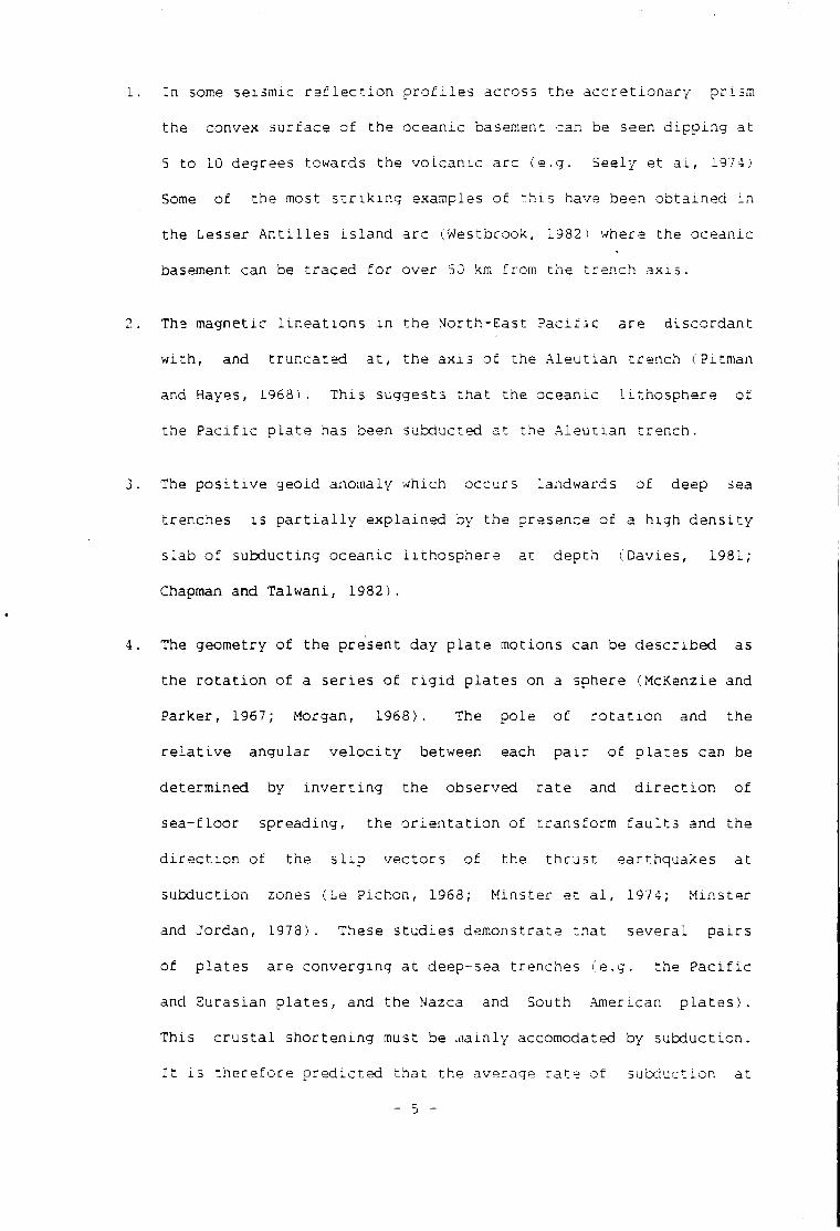
In some seismic r e f l e c t i o n p r o f i l e s across the a c c r e t i o n a r y prism
the convex surface of the oceanic basement can be seen d i p p i n g at
5 to 10 degrees towards the v o l c a n i c arc (e.g. Seely et a l , 1974)
Some of the most s t r i k i n g examples of t h i s have been obtained i n
the Lesser A n t i l l e s i s l a n d arc (Westbrook, 1982) where the oceanic
basement can be traced f o r over 50 km from the trench a x i s .
The magnetic l m e a t i o n s i n the North-East P a c i f i c are discordant
w i t h , and truncated a t , the ax i s of the A l e u t i a n trench (Pitman
and Hayes, 1968). This suggests t h a t the oceanic l i t h o s p h e r e of
the P a c i f i c p l a t e has been subducted at the A l e u t i a n trench.
The p o s i t i v e geoid anomaly which occurs landwards of deep sea
trenches i s p a r t i a l l y explained by the presence of a high d e n s i t y
slab of subducting oceanic i i t h o s p h e r e at depth (Davies, 1981;
Chapman and Talwani, 1982).
The geometry of the present day p l a t e motions can be described as
the r o t a t i o n of a series of r i g i d p l a t e s on a sphere (McKenzie and
Parker, 1967; Morgan, 1968). The pole of r o t a t i o n and the
r e l a t i v e angular v e l o c i t y between each p a i r of p l a t e s can be
determined by i n v e r t i n g the observed r a t e and d i r e c t i o n of
sea-floor spreading, the o r i e n t a t i o n of transform f a u l t s and the
d i r e c t i o n of the s l i p vectors of the t h r u s t earthquakes at
subduction zones (Le Pichon, 1968; Minster et a l , 1974; Minster
and Jordan, 1978). These studies demonstrate t h a t several p a i r s
of p l a t e s are converging at deep-sea trenches (e.g. the P a c i f i c
and Eurasian p l a t e s , and the Nazca and South American p l a t e s ) .
This c r u s t a l shortening must be aiainly accomodated by subduction.
I t i s t h e r e f o r e p r e d i c t e d t h a t the average r a t e of su'cduction at
the deep sea trenches which border the P a c i f i c i s about 9 cm/yr.
1.2 Morphology And Deep S t r u c t u r e Of Subduction Zones
In t h i s t h e s i s the term subduction zone i s used i n i t s broadest sense
to describe the wide range of feat u r e s which are produced by,, or associated
w i t h , the subduction of oceanic l i t h o s p h e r e . Subduction zones have
c h a r a c t e r i s t i c morphological f e a t u r e s which are continuous f o r thousands of
kilom e t r e s along t h e i r s t r i k e . The ma]or s t r u c t u r a l u n i t s w i l l t h e r e f o r e
be d e f i n e d by d e s c r i b i n g a cross se c t i o n through a t y p i c a l subduction zone.
The evidence discussed i n Section 1.1 suggests t h a t a subduction zone
i s formed where two l i t h o s p h e r i c p l a t e s , of which at l e a s t one i s oceanic,
are converging. These two p l a t e s are r e f e r r e d to as the subducting and
o v e r l y i n g p l a t e s . The subducting p l a t e i s d e f i n e d as the p l a t e which i s
bent i n t o the mantle, w h i l s t the o v e r l y i n g p l a t e i s the one which o v e r r i d e s
the subducting p l a t e and s u f f e r s l i t t l e v e r t i c a l displacement. The
subducting p l a t e i s always composed of oceanic l i t h o s p h e r e . This i s
because c o n t i n e n t a l l i t h o s p h e r e has a t h i c k low d e n s i t y c r u s t which i s too
buoyant to be subducted (McKenzie, 1969). The o v e r l y i n g p l a t e , however,
can be composed of e i t h e r oceanic or c o n t i n e n t a l l i t h o s p h e r e . Where the
o v e r l y i n g p l a t e i s oceanic we r e f e r to i t as an i s l a n d arc subducticn zone,
and where the o v e r l y i n g p l a t e i s c o n t i n e n t a l we r e f e r to i t as an a c t i v e
c o n t i n e n t a l margin subduction zone. I s l a n d arcs are common i n the West
P a c i f i c w h i l s t a c t i v e c o n t i n e n t a l margins are common i n the East P a c i f i c .
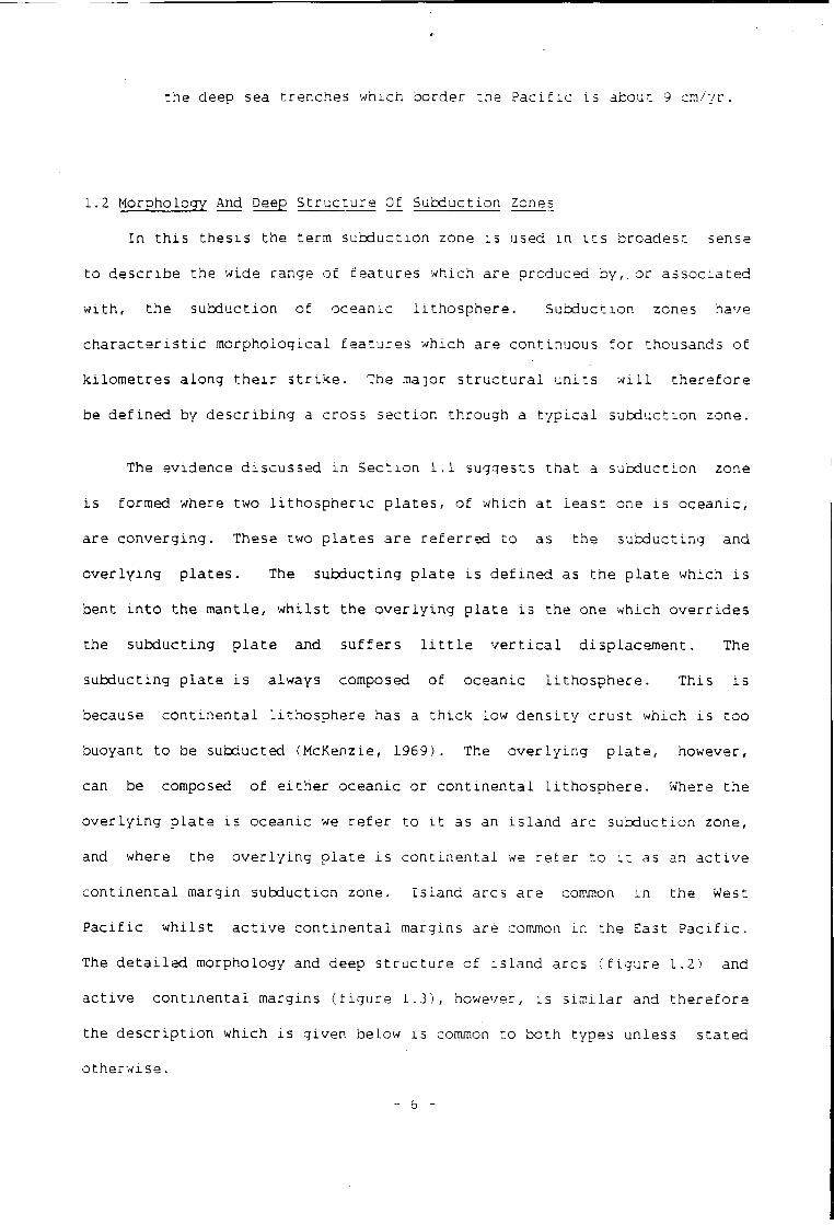
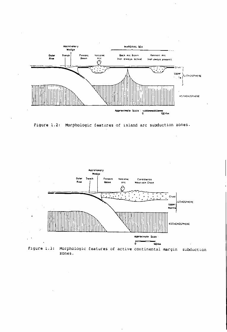
The d e t a i l e d morphology and deep s t r u c t u r e of i s l a n d arcs ( f i g u r e 1.2) and
a c t i v e c o n t i n e n t a l margins ( f i g u r e 1.3), however, i s s i m i l a r and t h e r e f o r e
the d e s c r i p t i o n which i s given below i s common to both types unless s t a t e d
otherwi se.
- 6 -
A c c r e h o n o r /
W e d g . M A R G I N A L S E A
O u t « r T r e n c h
R i t a F o r e o r c V o l c a n i c
S a t i n A r c
S a c k A r c B a s i n R « m n a n l A r c
I n o t a l w a y s a c l i v e l I n o l o l w a y t p r e s e n ! )
U p p e r / U T H O S P H E R E
A S 7 H E N 0 S P H E R E
A p p r a n i m a l t S e a l * 100 K m
Figure 1.2: Morphologic f e a t u r e s of i s l a n d arc subduction zones,
A c c r e l i o n a r y
W e d r g e
O u t e r T r t n c h F o r e a r c
R i s « 1 B a s i n M o u n t a i n C h a i n
C r u s t
M a n t l e
U T H O S P H E R E
Figure 1.3:
A S T H E N O S P H E f i E
A p p r o * i m o t « S c a l e .
0 ttOKm
Morphologic f e a t u r e s of a c t i v e c o n t i n e n t a l margin subduction zones.
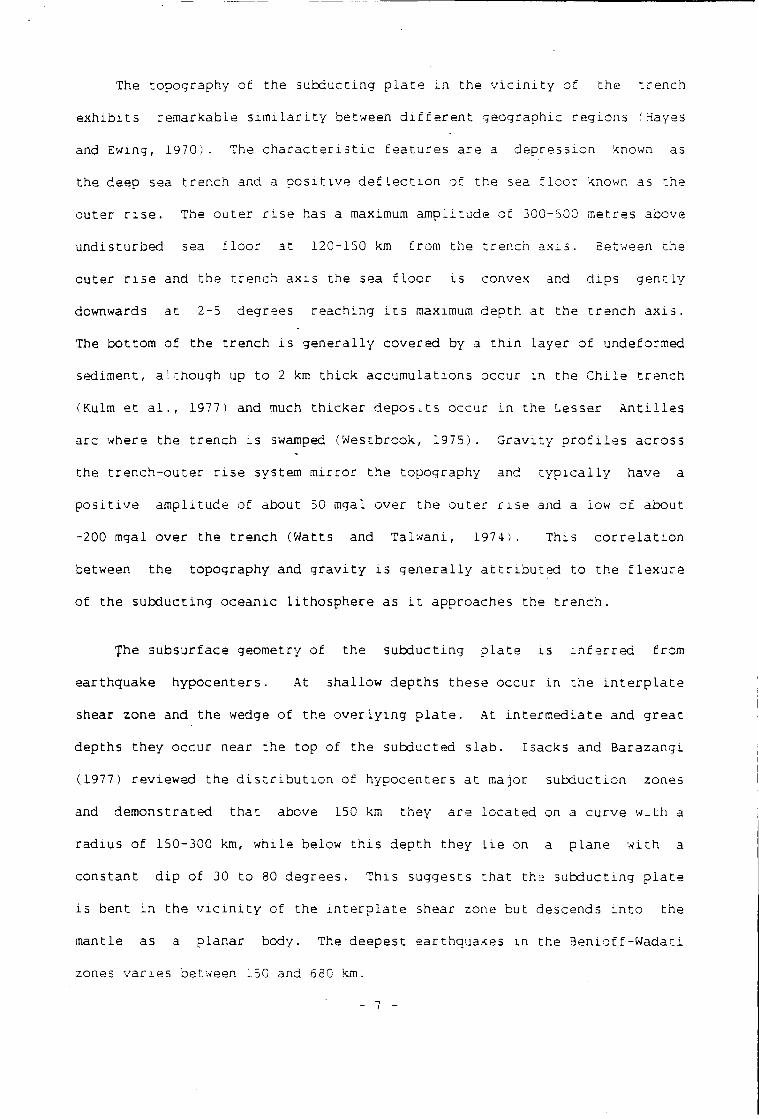
The topography of the subducting p l a t e i n the v i c i n i t y of the trench
e x h i b i t s remarkable s i m i l a r i t y between d i f f e r e n t geographic regions (Hayes
and Ewing, 1970) . The c h a r a c t e r i s t i c f e a t u r e s are a depression known as
the deep sea trench and a p o s i t i v e d e f l e c t i o n of the sea f l o o r known as the
outer r i s e . The outer r i s e has a maximum amplitude of 300-500 metres above
undisturbed sea f l o o r at 120-150 km from the trench a x i s . Between the
outer r i s e and the trench a x i s the sea f l o o r i s convex and dips g e n t l y
downwards at 2-5 degrees reaching i t s maximum depth at the trench a x i s .
The bottom of the trench i s g e n e r a l l y covered by a t h i n layer of undeformed
sediment, although up t o 2 km t h i c k accumulations occur i n the C h i l e trench
(Kulm et a l . , 1977) and much t h i c k e r d e p o s i t s occur i n the Lesser A n t i l l e s
arc where the trench i s swamped (Westbrook, 1975). G r a v i t y p r o f i l e s across
the trench-outer r i s e system m i r r o r the topography and t y p i c a l l y have a
p o s i t i v e amplitude of about 50 mgal over the outer r i s e and a low of about
-200 mgal over the trench (Watts and Taiwani, 1974). This c o r r e l a t i o n
between the topography and g r a v i t y i s g e n e r a l l y a t t r i b u t e d to the f l e x u r e
of the subducting oceanic l i t h o s p h e r e as i t approaches the tre n c h .
The subsurface geometry of the subducting p l a t e i s i n f e r r e d from
earthquake hypocenters. At shallow depths these occur i n the i n t e r p l a t e
shear zone and the wedge of the o v e r l y i n g p l a t e . At i n t e r m e d i a t e and great
depths they occur near the top of the subducted slab. Isacks and Barazangi
(1977) reviewed the d i s t r i b u t i o n of hypocenters a t major subduction zones
and demonstrated t h a t above 150 km they are located on a curve w i t h a
radius of 150-300 km, while below t h i s depth they l i e on a plane w i t h a
constant d i p of 30 to 80 degrees. This suggests t h a t the subducting p l a t e
i s bent i n the v i c i n i t y of the i n t e r p l a t e shear zone but descends i n t o the
mantle as a planar body. The deepest earthquakes i n the Benioff-Wadati
zones v a r i e s between 150 and 680 km.
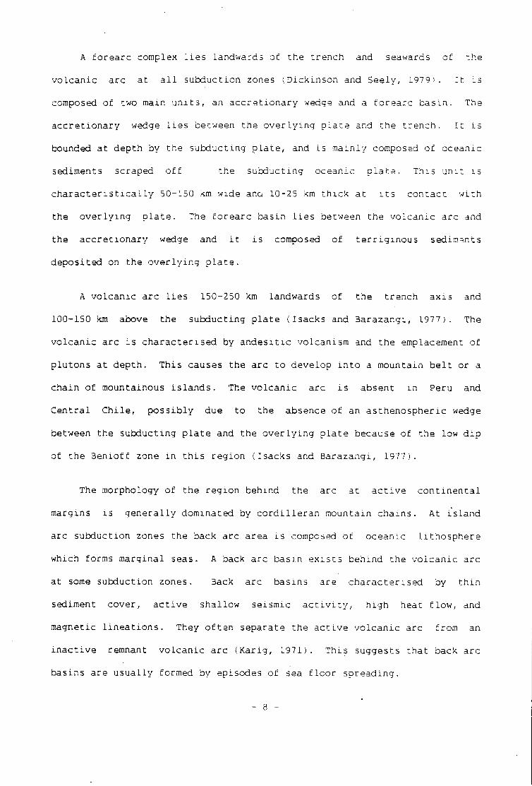
A f o r e a r c complex l i e s landwards of the trench and seawards of the
v o l c a n i c arc at a l l subduction zones (^Dickinson and Seely, 1979 ) . I t i s
composed of two main u n i t s , an a c c r e t i o n a r y wedge and a f o r e a r c basin. The
a c c r e t i o n a r y wedge l i e s between the o v e r l y i n g p l a t e and the trench. I t i s
bounded at depth by the subducting p l a t e , and i s mainly composed of oceanic
sediments scraped o f f the subducting oceanic p l a t e . This u n i t i s
c h a r a c t e r i s t i c a l l y 50-150 km wide ana 10-25 km t h i c k at i t s contact w i t h
the o v e r l y i n g p l a t e . The f o r e a r c basin l i e s between the v o l c a n i c arc and
the a c c r e t i o n a r y wedge and i t i s composed of t e r r i g i n o u s sediments
deposited on the o v e r l y i n g p l a t e .
A v o l c a n i c arc l i e s 150-250 km landwards of the trench a x i s and
100-150 km above the subducting p l a t e (Isacks and Barazangi, 1977). The
v o l c a n i c arc i s c h a r a c t e r i s e d by a n d e s i t i c volcanism and the emplacement of
plutons at depth. This causes the arc t o develop i n t o a mountain b e l t or a
chain of mountainous i s l a n d s . The v o l c a n i c arc i s absent i n Peru and
C e n t r a l C h i l e , p o s s i b l y due t o the absence of an asthenospheric wedge
between the subducting p l a t e and the o v e r l y i n g p l a t e because of the low d i p
of the 3 e n i o f f zone i n t h i s region (Isacks and Barazangi, 1977).
The morphology of the region behind the arc at a c t i v e c o n t i n e n t a l
margins i s g e n e r a l l y dominated by c o r d i l l e r a n mountain chains. At i s l a n d
arc subduction zones the back arc area i s composed of oceanic l i t h o s p h e r e
which forms marginal seas. A back arc basin e x i s t s behind the v o l c a n i c arc
at some subduction zones. Back arc basins are c h a r a c t e r i s e d by t h i n
sediment cover, a c t i v e shallow seismic a c t i v i t y , high heat flow, and
magnetic l i n e a t i o n s . They o f t e n separate the a c t i v e v o l c a n i c arc from an
i n a c t i v e remnant v o l c a n i c arc ( K a r i g , 1971). This suggests t h a t back arc
basins are u s u a l l y formed by episodes of sea f l o o r spreading.
- 3 -
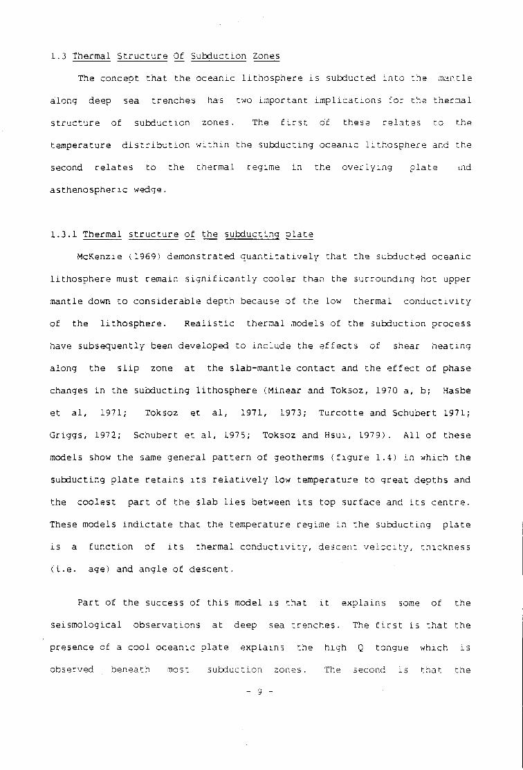
1.3 Thermal S t r u c t u r e Of Subduction Zones
The concept th a t the oceanic l i t h o s p h e r e i s subducted i n t o the mantle
along deep sea trenches has two important i m p l i c a t i o n s f o r the thermal
s t r u c t u r e of subduction zones. The f i r s t of these r e l a t e s to the
temperature d i s t r i b u t i o n w i t h i n the subducting oceanic l i t h o s p h e r e and the
second r e l a t e s to the thermal regime i n the o v e r l y i n g p l a t e md
asthenospheric wedge.
1.3.1 Thermal s t r u c t u r e of the subducting p l a t e
McKenzie (1969) demonstrated q u a n t i t a t i v e l y t h a t the subducted oceanic
l i t h o s p h e r e must remain s i g n i f i c a n t l y cooler than the surrounding hot upper
mantle down to considerable depth because of the low thermal c o n d u c t i v i t y
of the l i t h o s p h e r e . R e a l i s t i c thermal models of the subduction process
have subsequently been developed to include the e f f e c t s of shear h e a t i n g
along the s l i p zone at the slab-mantle contact and the e f f e c t of phase
changes i n the subducting l i t h o s p h e r e (Minear and Toksoz, 1970 a, b; Hasbe
et a l , 1971; Toksoz et a l , 1971, 1973; T u r c o t t e and Schubert 1971;
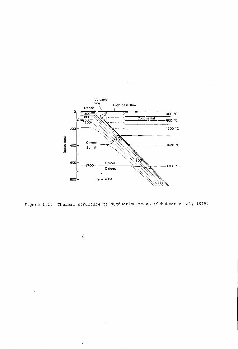
Griggs, 1972; Schubert et a l , 1975; Toksoz and Hsui, 1979). A l l of these
models show the same general p a t t e r n of geotherms ( f i g u r e 1.4) i n which the
subducting p l a t e r e t a i n s i t s r e l a t i v e l y low temperature to great depths and
the coolest p a r t of the slab l i e s between i t s top surface and i t s c e n t r e .
These models i n d i c t a t e t h a t the temperature regime i n the subducting p l a t e
i s a f u n c t i o n of i t s thermal c o n d u c t i v i t y , descent v e l o c i t y , thickness
( i . e . age) and angle of descent.
Part of the success of t h i s model i s that i t explains some of the
seismological observations at deep sea trenches. The f i r s t i s t h a t the
presence of a cool oceanic p l a t e explains the high Q tongue which i s
observed beneath most subduction zones. The second i s t h a t the
Volcanic line High heat flow
Trench \ 0
400 400 °C Continental \ Oceanic 800 °C
1200 °C 200
600 Olivine
1600 °C £ 400 Spinel \
6 0 0 Spinel 1700 1700 °C
Oxides
True scale 8 0 0
Figure 1 . 4 : Thermal s t r u c t u r e of subduction zones (Schubert et a l , 1975)
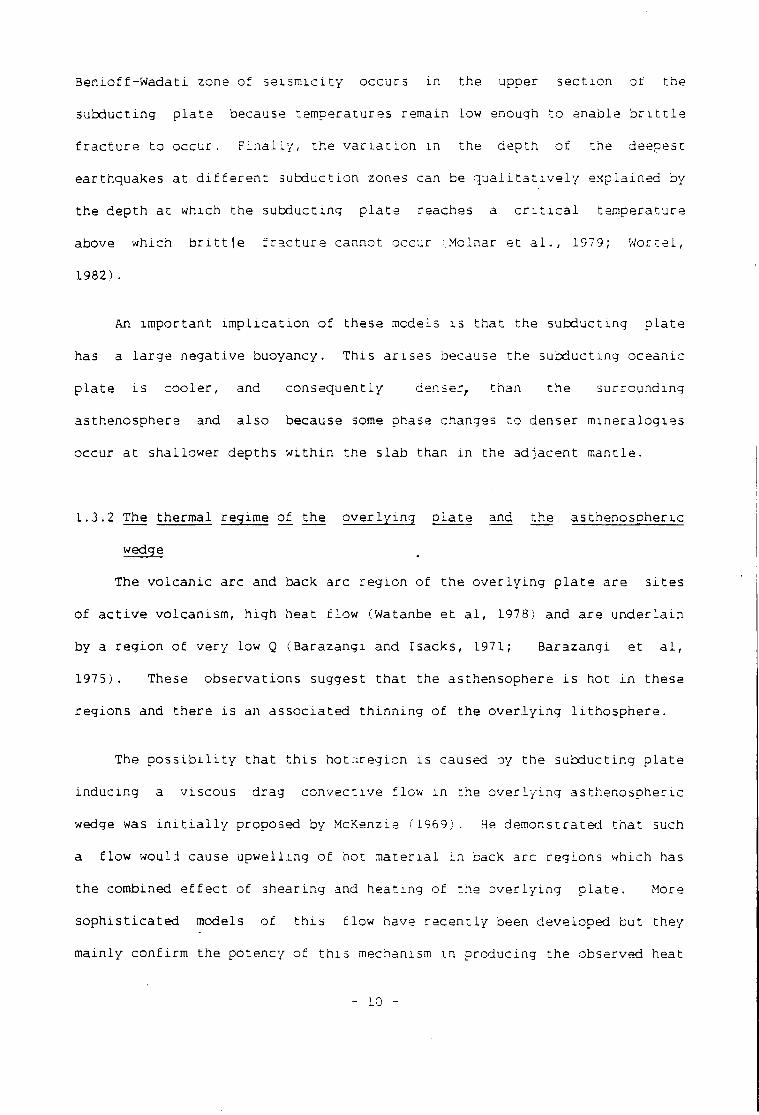
Benioff-Wadati zone of s a i s m i c i t y occurs i n the upper s e c t i o n of the
subducting p l a t e because temperatures remain low enough t o enable b r i t t l e
f r a c t u r e to occur. F i n a l l y , the v a r i a t i o n i n the depth of the deepest
earthquakes at d i f f e r e n t subduction zones can be q u a l i t a t i v e l y explained by
the depth at which the subducting p l a t e reaches a c r i t i c a l temperature
above which b r i t t l e f r a c t u r e cannot occur •: Molnar et a l . , 1979; Wortel,
1982) .
An important i m p l i c a t i o n of these models i s t h a t the subducting p l a t e
has a l a r g e negative buoyancy. This a r i s e s because the subducting oceanic
p l a t e i s c o o l e r , and consequently denser, than the surrounding
asthenosphere and also because some phase changes to denser mineralogies
occur at shallower depths w i t h i n the slab than i n the adjacent mantle.
1.3.2 The thermal regime of the o v e r l y i n g p l a t e and the asthenospheric
wedge
The v o l c a n i c arc and back arc re g i o n of the o v e r l y i n g p l a t e are s i t e s
of a c t i v e volcanism, high heat flow (Watanbe et a l , 1978) and are u n d e r l a i n
by a r e g i o n of very low Q (Barazangi and I sacks, 1971; Barazangi et a l ,
1975). These observations suggest t h a t the asthensophere i s hot i n these
regions and there i s an associated t h i n n i n g of the o v e r l y i n g l i t h o s p h e r e .
The p o s s i b i l i t y t h a t t h i s hot.-region i s caused by the subducting p l a t e
inducing a viscous drag convective flow i n the o v e r l y i n g asthenospherIC
wedge was i n i t i a l l y proposed by McKenzie (1969). He demonstrated t h a t such
a flow would cause upwelling of hot m a t e r i a l i n back arc regions which has
the combined e f f e c t of shearing and heating of the o v e r l y i n g p l a t e . More
s o p h i s t i c a t e d models of t h i s flow have r e c e n t l y been developed but they
mainly c o n f i r m the potency of t h i s mechanism i n producing the observed heat
- 10 -
flow i n back arc regions (.e.g. Toksoz and Hsui, 1978). These authors have
i m p l i e d from these models t h a t t h i s flow could also provide the ma]or
d r i v i n g force of back arc spreading.
An a d d i t i o n a l process which may c o n t r i b u t e tc the development of the
hot, very low Q zone i n the asthenospheric wedge and the surface a n d e s i t i c
"O.lcanism i s the release of water from the subducted oceanic c r u s t
(Ringwood, 1977).
1.4 The Observed State Of Stress At Subduction Zones
The f i r s t aim of t h i s s e c t i o n i s t o review the observed s t a t e of
stress at subduction zones. These observations w i l l be used to c o n s t r a i n
the models which w i l l be developed i n chapter 7. Th-e second aim i s to
review c u r r e n t ideas on the o r i g i n of the stress regime a t subduction
zones-.
The present-day s t a t e of stress i n the the l i t h o s p h e r e can be
determined by three main methods. The f i r s t i s to i n f e r the p r i n c i p a l
stress o r i e n t a t i o n s from the f o c a l mechanisms of earthquakes. This method
can only be used i n l i m i t e d areas, such as new p l a t e boundaries, which are
s e i s m i c a l l y a c t i v e . The second method i s t o i n f e r the p r i n c i p a l s tress
o r i e n t a t i o n from stress s e n s i t i v e g e o l o g i c a l s t r u c t u r e s . This method
requires r e l i a b l e d a t i n g of the s t r u c t u r e s and i s r e s t r i c t e d to
g e o g r a p h i c a l l y accessible areas, but i t i s u s e f u l i n regions where f o c a l
mechanism studies are absent. The t h i r d method i s to evaluate the s t r e s s
regime using i n s i t u techniques (McGarr and Gay, 1978). These methods are
r e s t r i c t e d t o g e o g r a p h i c a l l y accessible areas and have not been a p p l i e d at
subduction zones.
- 11 -
The subducting p l a t e and the leading edge of the o v e r l y i n g p l a t e are
both s e i s m i c a l l y a c t i v e and consequently t h e i r s tress regime can g e n e r a l l y
be i n f e r r e d from seismic f o c a l mechanism s o l u t i o n s . The oack arc area,
however, i s less s e i s m i c a l l y a c t i v e and consequently the stress regime L S
p r i n c i p a l l y i n f e r r e d from stress s e n s i t i v e g e o l o g i c a l f e a t u r e s .
The s t a t e of stress i s observed to be r e g i o n a l l y c o n s i s t e n t along the
s t r i k e of subduction zones. The stress regime at subduction zones can
t h e r e f o r e be adequately modelled i n two dimensions. The observed s t a t e of
stress i s consequently described i n t h i s s e c t i o n as a two dimensional cross
sec t i o n through the t e c t o n i c provinces of a subduction zone.
1.4.1 Trench-outer r i s e system
Seismic r e f l e c t i o n p r o f i l e s show t h a t the seismic basement and
o v e r l y i n g sediments i n the trench-outer r i s e system are d i s s e c t e d by
numerous normal f a u l t s (Ludwig et a l , 1973). The earthquakes i n t h i s area
are located a t depths of less than 25 km and are i n f e r r e d from t h e i r f o c a l
mechanism s o l u t i o n s to be produced by h o r i z o n t a l t e n s i o n a l stresses which
are o r i e n t a t e d normal to the trench a x i s (Chappie and Forsyth, 1979). This
stress p a t t e r n i s g e n e r a l l y considered t o r e s u l t from the f l e x u r e of the
oceanic l i t h o s p h e r e as i t i s bent i n t o the subduction zone (e.g. Watts and
Talwani, 1974).
Recently, however, Christensen and Ruff (1983) have presented evidence
which suggests t h a t the s t a t e of stress i n t h i s r e g i o n may be more
complicated. They demonstrated t h a t a small number of compressional
earthquakes are observed i n the shallow p o r t i o n of the subducting p l a t e
p r i o r t o major subduction zone earthquakes. This evidence suggests t h a t
h o r i z o n t a l compressive stress may b u i l d up i n the trench-outer r i s e
- 12 -
immediately before major u n d e r t h r u i t i n g occurs.
1.4.2 The leading edge of the o v e r l y i n g p l a t e
The leading edge of the o v e r l y i n g p l a t e , which comprises the region
between the trench a x i s and the v o l c a n i c arc, i s the most s e i s m i c a l l y
a c t i v e environment i n the world. I t i s c h a r a c t e r i s e d by numerous shallow
earthquakes. Kanamori (1977) demonstrated t h a t ten great earthquakes
(magnitude greater than 7.5) r e l e a s i n g over 90% of the worlds t o t a l seismic
energy occurred i n t h i s r e g i o n between 1904 and 1976. He also demonstrated
th a t these earthquakes occurred predominantly on low angle t h r u s t f a u l t s .
The numerous smaller magnitude earthquakes which occur i n t h i s region are
also considered to be produced by t h r u s t f a u l t s (Stauder, 1968; 1975).
Seismic r e f l e c t i o n p r o f i l e s across the sedimentary wedge have also shown
th a t the major s t r u c t u r a l f e a t u r e s i n t h i s region are landward d i p p i n g
t h r u s t f a u l t s (Dickenson and Seely, 1979) .
The observation t h a t the deformation at the l e a d i n g edge of the
o v e r l y i n g p l a t e occurs almost e x c l u s i v e l y on low angle t h r u s t f a u l t s
suggests t h a t the p r i n c i p a l s tress i n t h i s r e g i o n i s predominantly
h o r i z o n t a l compression o r i e n t a t e d perpendicular t o the trench a x i s . I t i s
g e n e r a l l y considered t h a t t h i s s t r e s s regime i s caused by the r e l a t i v e
motion of the two converging p l a t e s (e.g. Isacks et a l , 1968). This
i n t e r p r e t a t i o n i s supported by the observed surface deformation which
f o l l o w s l a rge t h r u s t earthquakes (e.g. P l a f k e r , 1965).
Kanamori (1977) demonstrated t h a t the magnitude of the compression i n
t h i s r egion may vary between subduction zones. He has shown t h a t :
- 13 -
1. Great t h r u s t earthquakes are s p a t i a l l y concentrated at c e r t a i n
subduction zones.
2. At the subduction zones where great t h r u s t earthquakes occur (.e.g.
C h i l e , Alaska, the Al e u t i a n s and Kuril-Kamchatka) the seismic s l i p
r a t e (estimated from the displacement on the r u p t u r e plane and the
recurrence time) i s equal to the displacement p r e d i c t e d by the
kinematic p l a t e motions. These subduction zones c o r r e l a t e w i t h
strong r e g i o n a l compression i n the o v e r l y i n g p l a t e .
3. At subduction zones where great earthquakes do not occur (e.g the
Marianas, Izu-Bonin, Java-Sumatra and Tonga-Kermadec), the seismic
s l i p r a t e i s less than the displacement p r e d i c t e d by the kinematic
models of p l a t e motion. These subduction zones are c h a r a c t e r i s e d
by t e n s i o n a l s t r e s s i n the back arc areas.
Kanamori has explained these observations by a model i n which the
degree of mechanical c o u p l i n g of the p l a t e s v a r i e s between subduction
zones. He suggested t h a t where the c o u p l i n g i s strong great earthquakes
occur and the stress i s r e g i o n a l compression, but where the co u p l i n g i s
weak great earthquakes are absent and t e n s i o n a l stresses may occur i n the
back arc areas. This model suggests t h a t the mechanical coupling between
the p l a t e s c o n t r o l s the amount of compression which i s t r a n s m i t t e d i n t o the
o v e r l y i n g p l a t e .
Ruff and Kanamori (1983a, 1983b) demonstrated t h a t the t h r u s t
earthquakes at coupled subduction zones have r e l a t i v e l y l a r g e r a s p e r i t i e s
(regions r e s i s t i n g motion on the f a u l t plane) than those at uncoupled
subduction zones. They suggested t h a t the magnitude of the h o r i z o n t a l
compressive stress at the leading edge of the o v e r l y i n g p l a t e i s
- 14 -
p r o p o r t i o n a l t o the r a t i o of the area of the a s p e r i t e s to the t o t a l area of
the f a u l t plane.
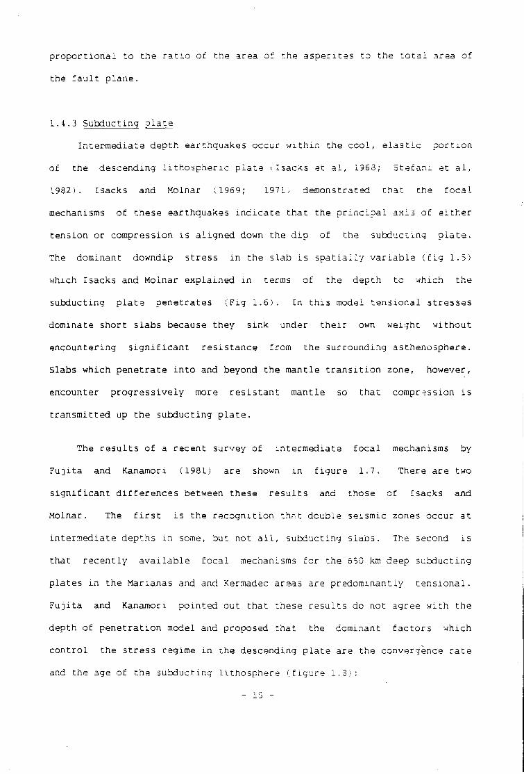
1.4.3 Subducting p l a t e
Intermediate depth earthquakes occur w i t h i n the c o o l , e l a s t i c p o r t i o n
of the descending i i t h o s p h e r i c p l a t e (Isacks et a l , 1963; S t e f a n i et a l ,
1982). Isacks and Molnar (1969; 1971; demonstrated t h a t the f o c a l
mechanisms of these earthquakes i n d i c a t e t h a t the p r i n c i p a l a xis of e i t h e r
tension or compression i s a l i g n e d down the d i p of the subducting p l a t e .
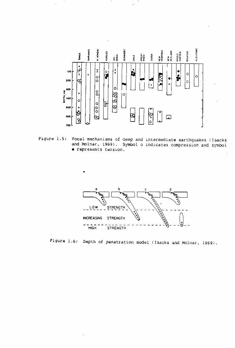
The dominant downdip stress i n the slab i s s p a t i a l l y v a r i a b l e ( f i g 1.5)
which Isacks and Molnar explained i n terms of the depth to which the
subducting p l a t e penetrates ( F i g 1.6). I n t h i s model t e n s i o n a l stresses
dominate short slabs because they sink under t h e i r own weight w i t h o u t
encountering s i g n i f i c a n t r e s i s t a n c e from the surrounding asthenosphere.
Slabs which penetrate i n t o and beyond the mantle t r a n s i t i o n zone, however,
en'counter p r o g r e s s i v e l y more r e s i s t a n t mantle so t h a t compression i s
t r a n s m i t t e d up the subducting p l a t e .
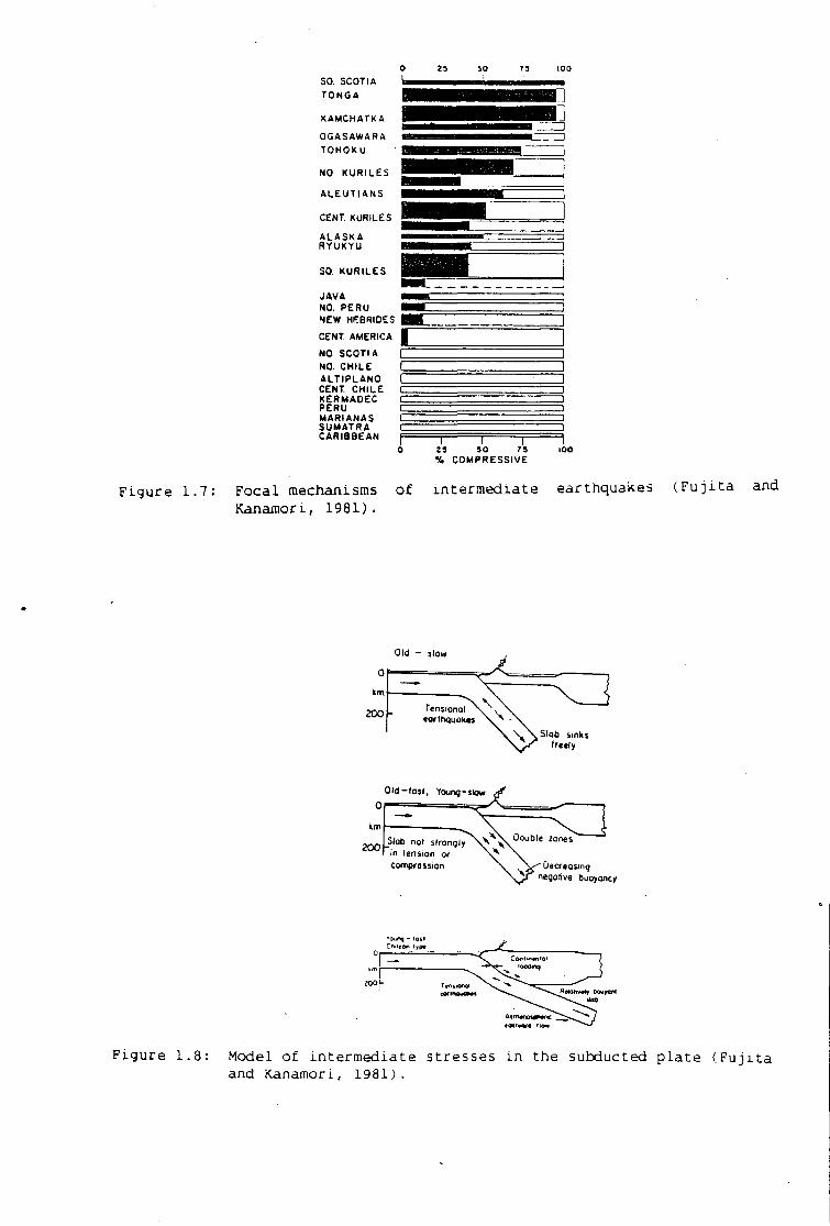
The r e s u l t s of a recent survey of i n t e r m e d i a t e f o c a l mechanisms by
F u j i t a and Kanamori (1981) are shown i n f i g u r e 1.7. There are two
s i g n i f i c a n t d i f f e r e n c e s between these r e s u l t s and those of Isacks and
Molnar. The f i r s t i s the r e c o g n i t i o n t h a t double seismic zones occur at
intermediate depths i n some, but not a l l , subducting slabs. The second i s
t h a t r e c e n t l y a v a i l a b l e f o c a l mechanisms f o r the 550 km deep subducting
pl a t e s i n the Marianas and and Kermadec areas are predominantly t e n s i o n a l .
F u j i t a and Kanamori pointed out t h a t these r e s u l t s do not agree w i t h the
depth of p e n e t r a t i o n model and proposed t h a t the dominant f a c t o r s which
c o n t r o l the s t r e s s regime i n the descending p l a t e are the convergence r a t e
and the age of the subducting l i t h o s p h e r e ( f i g u r e 1.3):
- 15 -
2 3: 3 u
900
600
TOO
95
L Q J
O
o
o o
o o o °c
O o
o 3
6 !
ft 5? o
o
8
a
o c
Figure 1.5: Focal mechanisms of deep and inte r m e d i a t e earthquakes (Isacks and Molnar, 1969). Symbol o i n d i c a t e s compression and symbol • represents t e n s i o n .
L O W STRENGTH
INCREASING STRENGTH
HIGH S T R E N G T H
Figure 1.6: Depth of p e n e t r a t i o n model (Isacks and Molnar, 1969)
S O . S C O T I A
T O N G A
K A M C H A T K A
O G A S A W A R A
T O H O K U
N O K U R I L E S
A L E U T I A N S
C E N T . K U R I L E S
A L A S K A R Y U K Y U
S O K U R I L E S
J A V A
N O . P E R U
N E W H E B R I D E S
C E N T A M E R I C A
N O . S C O T I A
N O . C H I L E
A L T I P L A N O C E N T . C H I L E K E R M A O E C P E R U M A R I A N A S S U M A T R A C A R I B B E A N -\ i r
2 9 1 0 7 S
% C O M P R E S S I V E
Figure 1.7: Focal mechanisms of Kanamori, 1981).
inte r m e d i a t e earthquakes ( F u j i t a and
O l d s l o w
k m
T e n s i o n o l 2 0 0 e a r t h q u a k e s
f r e e l y
O l d - f a s t , Y o u n g - s t o w
k m
200 S l a t ) n o t s t r o n g l y
i n t e n s i o n o r
c o m p r e s s i o n
D o u b l e z o n e s
D e c r e a s i n g
n e g a t i v e b u o y a n c y
rot^o - (at Cnnton tyD* 2 ContwtfttQl
2 0 0 r MI n a n a corinautno*
A i i n c n o u r w i C *<Hi«o(d flow
Figure 1.8: Model of i n t e r m e d i a t e stresses i n the subducted p l a t e ( F u j i t a and Kanamori, 1981).
1. Old and slow slabs: The s t a t e of stress i n o l d slabs w i t h a low
convergence r a t e i s dominantly t e n s i o n a l . This i s because the o l d
l i t h o s p h e r e has a large negative buoyancy and t h e r e f o r e tends to
sink i n t o the mantle f a s t e r than the plates are converging. This
causes the subducting p l a t e to ' p u l l ' i t s e l f i n t o the mantle and
t h e r e f o r e t e n s i o n a i streses dominate i t .
2. Old and f a s t , and young and slow: These c o n d i t i o n s favour the
development of double seismic zones. This i s because the
convergence r a t e i s almost equivalent t o the age c o n t r o l l e d r a t e
at which the slab i s s i n k i n g i n t o the mantle and t h e r e f o r e l o c a l
effects such as unbending (Engdahl and Scholz, 1977), sagging
(Sleep, 1979), or thermal e f f e c t s ( V e i t h , 1977) dominate the
stress i n the slab and produce double seismic zones.
3. Young and f a s t : Under these c o n d i t i o n s compression dominates the
s i n k i n g p l a t e . This i s because the convergence r a t e i s f a s t e r
than the speed at which the slab i s s i n k i n g due to i t s negative
buoyancy, and t h e r e f o r e , the subducting p l a t e i s pushed i n t o the
mantle and i s consequently dominated by compressional stresses.
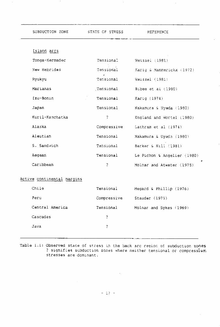
1.4.4 Back arc regions
Because of the l i m i t e d seismic a c t i v i t y i n the back arc areas of
subduction zones, the stress regime has to be p r i n c i p a l l y i n f e r r e d from
stress s e n s i t i v e g e o l o g i c a l f e a t u r e s and marine observations. These
observations have shown t h a t , u n l i k e other provinces associated w i t h
subduction zones the dominant h o r i z o n t a l p r i n c i p a l stress i n back arc areas
v a r i e s from region to region (Table 1.1).
- 16 -
SUBDUCTION ZONE STATE OF STRESS REFERENCE
Is l a n d arcs
Tonga-Kermadec
New Hebrides
Ryukyu
Marianas
Izu-Bonin
Japan
Kuril-Kamchatka
Alaska
A l e u t i a n
S. Sandwich
Aegean
Caribbean
Tensionai
Tensiorial
Tensionai
.Tensional
Tensional
Tensional
Compressive
Tensional
Tensional
Tensional
Weissel (.1981)
Karig & Mammerickx (1972)
Weissel (1981)
Bibee et a l (1980)
Karig (1974)
Nakamura & Uyeda (.1980)
England and Wortel (1980)
Lathram et a l (1974)
Nakamura & Uyeda (1980)
Barker & H i l l (1981)
Le Pichon & Angelier (1980)
Molnar and Atwater (1978)
A c t i v e c o n t i n e n t a l margins
C h i l e
Peru
Cent r a l America
Cascades
Java
Tensional
Compressive
Tensional
Megard & P h i l l i p (1976)
Stauder (1975)
Molnar and Sykes (1969)
Table 1.1: Observed s t a t e of stress i n the back arc region of subduction zones ? s i g n i f i e s subduction zones where n e i t h e r t e n s i o n a i or compression stresses are dominant.
- 17 -
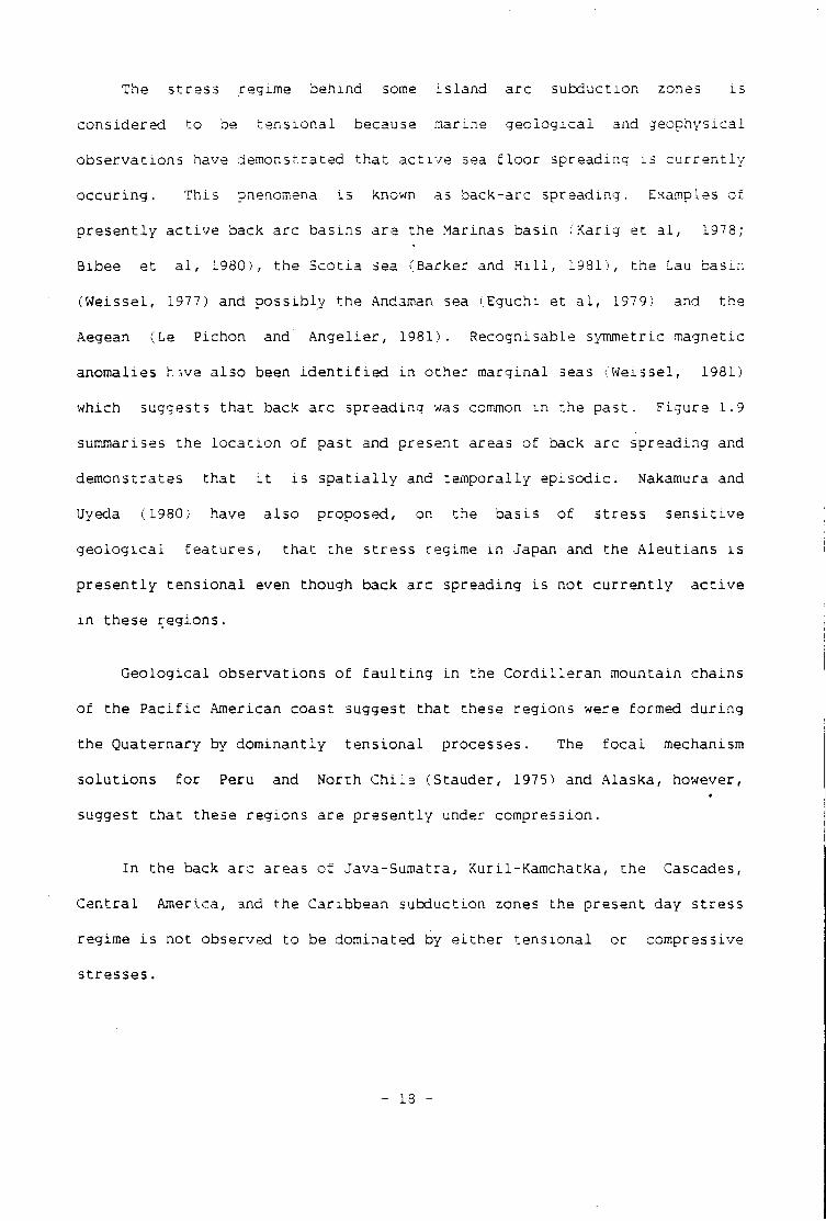
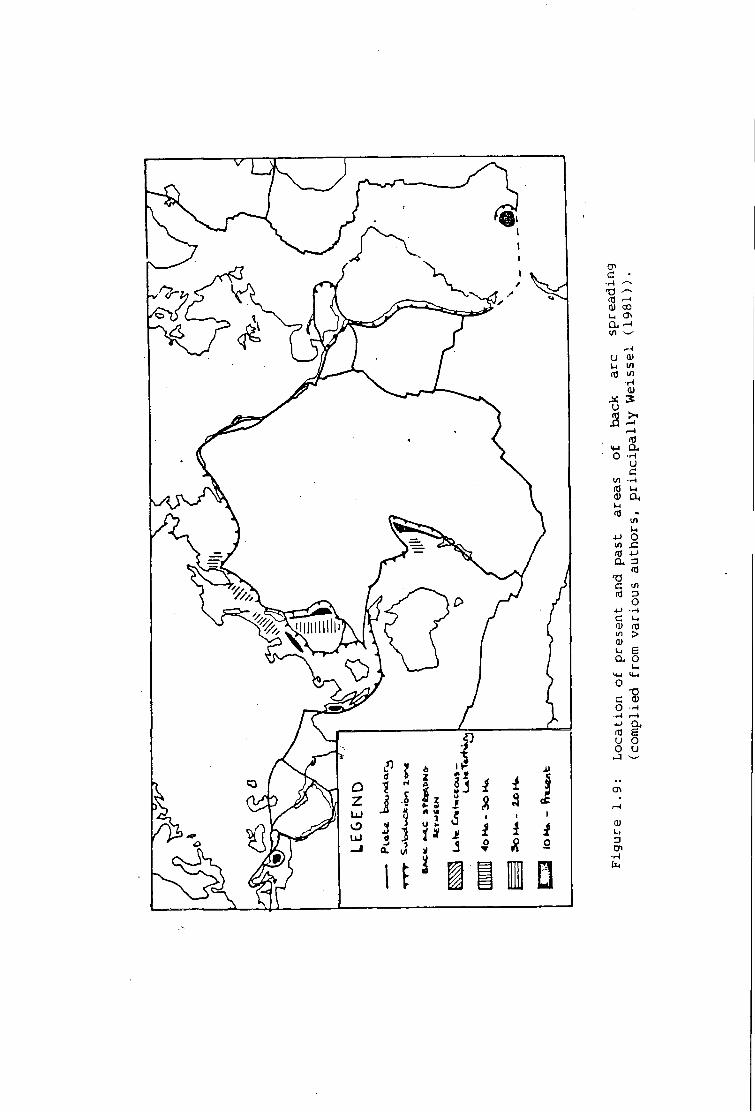
The stress regime behind some i s l a n d arc subduction zones i s
considered to be t e n s i o n a l because marine g e o l o g i c a l and geophysical
observations have demonstrated t h a t a c t i v e sea f l o o r spreading i s c u r r e n t l y
o c c u r i n g . This phenomena i s known as back-arc spreading. Examples of
p r e s e n t l y a c t i v e back arc basins are the Marinas basin ( K a r i g et a l , 1978;
Bibee et a l , 1980), the Scotia sea (Barker and H i l l , 1981), the Lau basin
(Weissel, 1977) and p o s s i b l y the Andaman sea (Eguchi et a l , 1979) and the
Aegean (Le Pichon and A n g e l i e r , 1981). Recognisable symmetric magnetic
anomalies have also been i d e n t i f i e d i n other marginal seas (Weissel, 1981)
which suggests t h a t back arc spreading was common i n the past. Figure 1.9
summarises the l o c a t i o n of past and present areas of back arc spreading and
demonstrates t h a t i t i s s p a t i a l l y and temporally e p i s o d i c . Nakamura and
Uyeda (1980) have also proposed, on the basis of stress s e n s i t i v e
g e o l o g i c a l f e a t u r e s , t h a t the s t r e s s regime i n Japan and the A l e u t i a n s i s
p r e s e n t l y t e n s i o n a l even though back arc spreading i s not c u r r e n t l y a c t i v e
i n these regions.
Geological observations of f a u l t i n g i n the C o r d i l l e r a n mountain chains
of the P a c i f i c American coast suggest t h a t these regions were formed d u r i n g
the Quaternary by dominantly t e n s i o n a l processes. The f o c a l mechanism
s o l u t i o n s f o r Peru and North Chi I a (Stauder, 197 5) and Alaska, however,
suggest t h a t these regions are p r e s e n t l y under compression.
In the back arc areas of Java-Sumatra, Kuril-Kamchatka, the Cascades,
Ce n t r a l America, and the Caribbean subduction zones the present day stress
regime i s not observed to be dominated by e i t h e r t e n s i o n a l or compressive
stresses.
- 18 -
{ 1 £
i
1 1 re
0 01
CP c • •l-l T3 ^ 01 '-' 0) CO
a ^ i/i ^
u <u
•H <D
X 3 u a s
r-l (T3
<M a. o H u c i/i a) Ou M m -
Ul u
4 J O i/i x: (0 -u a => m c </i
o C u <D n3 i/i > a> u e cx o i t
•4-1 lt-1 o
O — I f-H 4J a m e u o o u
Because the kinematics of the subduction process p r e d i c t s t h a t
subduction zones are s i t e s of c r u s t a l shortening they would be p r e d i c t e d to
be s i t e s of r e g i o n a l compression. The observations reviewed i n t h i s
s e c t i o n , however, demonstrate that tension i s more common i n back arc
regions. Several models have been proposed to e x p l a i n the o r i g i n of t h i s
t e n s i o n a l s t r e s s :
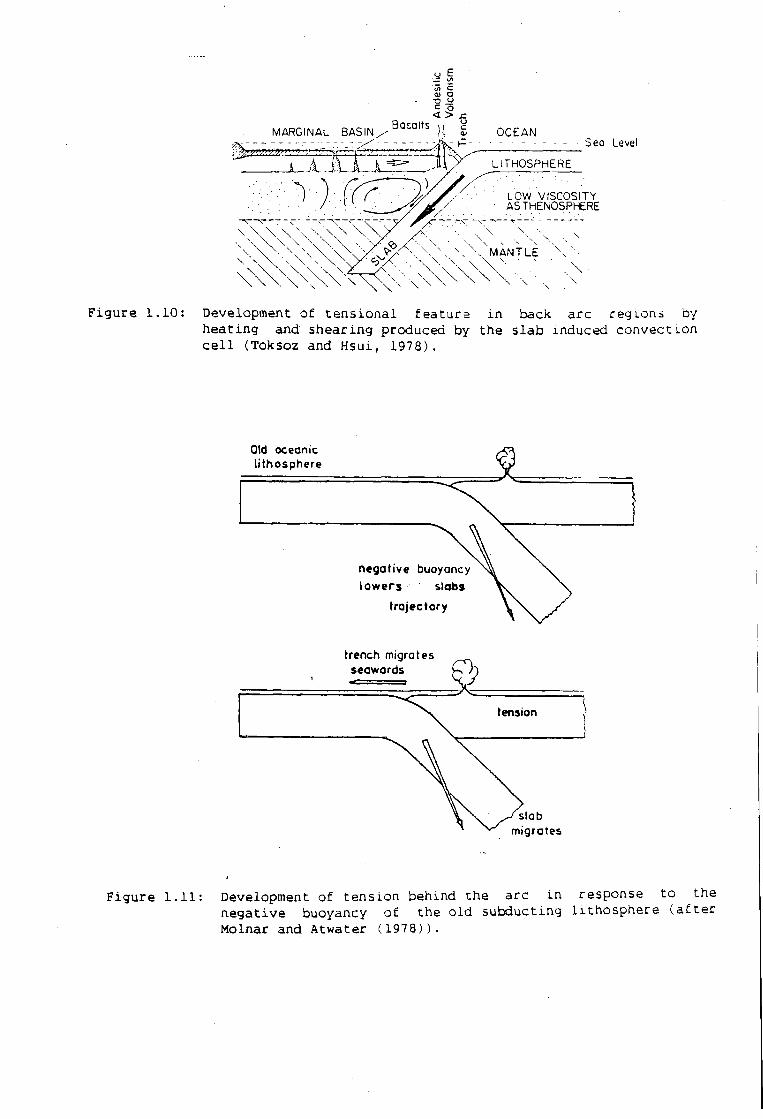
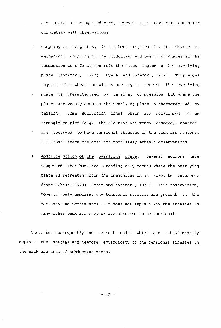
1. Slab induced, convection. Several authors have proposed t h a t the
tensi o n i n back arc basins, and more s p e c i f i c a l l y the f o r c e
d r i v i n g back arc spreading, i s produced by the combination of
heating and shearing which i s associated w i t h slab induced
convection (Figure 1.10). This mechanism should produce t e n s i o n a l
stresses at those subduction zones where the slab penetrates
deeper than several hundred k i l o m e t r e s . Because the
Kuril-Kamchatka and Java-Sumatra subduction zones have deep slabs
but are not t e n s i o n a l , t h i s p r e d i c t i o n i s ' not supported by
observations. A f u r t h e r l i m i t a t i o n of t h i s model i s t h a t i t does
not provide a s a t i s f a c t o r y mechanism to stop back arc spreading
other than by cessation of subduction.
2. Negative buoyancy• Observations i n d i c a t e t h a t compression i s
dominant i n regions where young slabs are being subducted and
tension where o l d slabs are being subducted. This suggests t h a t
the stress regime i n the o v e r l y i n g p l a t e may be c o n t r o l l e d by the
age of the subducting p l a t e because of the incr e a s i n g negative
buoyancy of the oceanic l i t h o s p h e r e as i t ages (Molnar and
Atwater, 1978; England and Wortel, 1980). Because the stresses
are t e n s i o n a l a t some subduction zones where very young slabs are
being subducted (e.g. C h i l e ) and are not t e n s i o n a l where every
- 19 -
u E S c 0> o •o -!=> c o < > -g
MARGINAL BASIN / B a £ a l t s )(, £ O C E A N Sea Level
THOSPHERE
LOW VISCOSITY ASTHENOSPHERE
M A N T L E
Figure 1.10: Development of t e n s i o n a l f e a t u r e i n back arc regions by heat i n g and shearing produced by the slab induced convection c e l l (Toksoz and Hsui, 1978).
Old oceanic l ithosphere
negative buoyancy l o w e r s slabs
trajectory
trench migrates seawards
tension
slab migrates
Figure 1.11: Development of ten s i o n behind the arc i n response t o the negative buoyancy of the o l d subducting l i t h o s p h e r e ( a f t e r Molnar and Atwater (1978)).
o l d p l a t e i s being subducted, however, t h i s model does not agree
completely w i t h observations.
3. Coupling of the p l a t e s . I t has been proposed t h a t the degree of
mechanical coupling of the subducting and o v e r l y i n g p l a t e s at the
subduction zone f a u l t c o n t r o l s the stress regime i n the o v e r l y i n g
p l a t e (Kana.no r i , 1977; Uyeda and Kan amor L, 1979). This mode]
sugg€;Str> t h a t where the p l a t e s are h i g h l y coupled the o v e r l y i n g
p l a t e i s c h a r a c t e r i s e d by r e g i o n a l compression but where the
p l a t e s are weakly coupled the o v e r l y i n g p l a t e i s c h a r a c t e r i s e d by
ten s i o n . Some subduction zones which are considered t o be
s t r o n g l y coupled (e.g. the A l e u t i a n and Tonga-Kermadec), however,
are observed t o have t e n s i o n a l stresses i n the back arc regions.
This model t h e r e f o r e does not completely explain observations.
4. Absolute motion of the o v e r l y i n g p l a t e . Several authors have
suggested that back arc spreading only occurs where the o v e r l y i n g
p l a t e i s r e t r e a t i n g from the t r e n c h l i n e i n an absolute reference
frame (Chase, 1978; Uyeda and Kanamori, 1979). This o b s e r v a t i o n ,
however, only explains why t e n s i o n a l stresses are present i n the
Marianas and Scotia arcs. I t does not exp l a i n why the stresses i n
many other back arc regions are observed t o be t e n s i o n a l .
There i s consequently no c u r r e n t model which can s a t i s f a c t o r i l y
e x p l a i n the s p a t i a l and temporal e p i s o d i c i t y of the t e n s i o n a l stresses i n
the back arc area of subduction zones.
- 20 -
1.5 Sources Of Stress
Stresses are produced i n the l i t h o s p h e r e by the a c t i o n of boundary and
body f o r c e s . The s t r e s s regime which these forces produce, i n p a r t i c u l a r
t h e i r response over time, i s con-.rolled by the rheology of the l i t h o s p h e r e .
The rheology of the l i t h o s p h e r e i s reviewed i n chapter 2 and i t i s
t h e r e f o r e the aim of t h i s s e c t i o n to review the sources of l i t h o s p h e r i c
s t r e s s .
The sources of s t r e s s i n an e l a s t i c l i t h s o p h e r e were reviewed by
T u r c o t t e and Oxburgh (1976). They considered t h a t the l i t h o s p h e r i c s t r e s s
regime i s the product of the system of boundary and body forces which
p r e s e n t l y act upon i t and the i n i t i a l s t r a i n s which were produced by
e a r l i e r t e c t o n i c events. Since then, however, several advances i n our
knowledge of the time dependent nature of the rheology of the l i t h o s p h e r e
have improved our understanding of the sources of t e c t o n i c s t r e s s . These
advances l e d Bott (1982a) t o r e c l a s s i f y the sources of l i t h o s p h e r i c s t r e s s
i n t o renewable or non-renewable stress systems. Renewable sources of
stress are produced by forces which continuously regenerate s t r a i n energy
(e.g. body forces and p l a t e d r i v i n g f o r c e s ) . Non-renewable stresses are
produced by i n i t i a l s t r a i n s which do not continuously generate s t r a i n
energy (e.g. thermal and bending s t r e s s e s ) . Unlike non-renewable s t r e s s ,
renewable stresses are not r e l i e v e d by t r a n s i e n t creep and they are
consequently subject to stress a m p l i f i c a t i o n i n the upper e l a s t i c layer of
the l i t h o s p h e r e (Kusznir and B o t t , 1977; Bott and Kusznir, 1979). The
forces which generate renewable stress are t h e r e f o r e the major sources of
t e c t o n i c s t r e s s i n the l i t h o s p h e r e .
The main sources of stress i n the l i t h o s p h e r e are:
- 21 -
Plate d r i v i n g f o r c e s . These force s , which are a renewable source
of s t r e s s , are of p l a t e t e c t o n i c o r i g i n (Forsyth and Uyeda, 1975).
They i n c l u d e ;
1. Ridge push. Which r e s u l t s from the continuous up w e l l i n g of
hot, low d e n s i t y m a t e r i a l beneath mid ocean rid g e s .
2. Slab p u l l . Which a r i s e s from the large negative buoyancy of
the c o o l , and consequently dense, subducting slab.
3. Trench s u c t i o n . This i s a f o r c e which p u l l s the o v e r l y i n g
p l a t e towards the subducting p l a t e (Elsasser, 1971). The
o r i g i n of trench s u c t i o n i s not w e l l understood. I t may
p o s s i b l y r e s u l t from the r o l l - b a c k of the subducting p l a t e
(Chase, 1978; Molnar and Atwater, 1978) or the shear stress
a r i s i n g from slab induced convection ( R i c h t e r , 1975).
These f o r c e s , which are probably the l a r g e s t of p l a t e t e c t o n i c
o r i g i n , are r e s i s t e d by viscous drag along the i n t e r f a c e of the
p l a t e s w i t h the mantle and by f r i c t i o n a l r e s i s t a n c e along
i n t e r p l a t e boundaries.
Loading f o r c e s . Body fo r c e s , r e s u l t i n g from the weight of the
l i t h o s p h e r e , produce l a r g e stresses i n the l i t h o s p h e r e . Important
d e v i a t o r i c stress regimes are produced where there are l o c a l
changes i n the magnitude of loading forces, e i t h e r r e s u l t i n g from
l a t e r a l v a r i a t i o n s i n the d e n s i t y of the l i t h o s p h e r e or from
changes i n the magnitude of topographic loads:
1. Topographic surface loads w i t h a short wavelength (.ess than
h a l f the thickness of the l i t h o s p h e r e ) do not r e s u l t i n
- 22 -
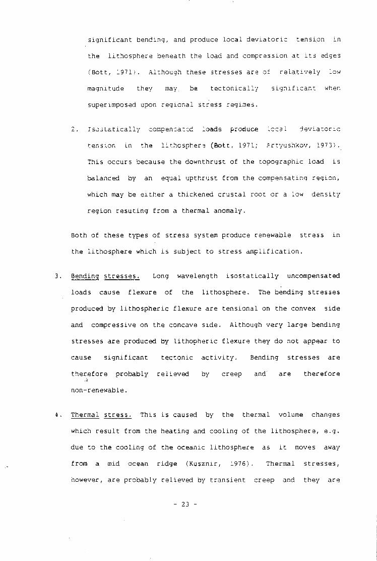
s i g n i f i c a n t bending, and produce l o c a l d e v i a t o r i c tension i n
the l i t h o s p h e r e beneath the load and compression at i t s edges
( B o t t , 1971). Although these stresses are of r e l a t i v e l y low
magnitude they may. be t e c t o n i c a l l y s i g n i f i c a n t ' when
superimposed upon r e g i o n a l stress regimes.
2. I s o j t a t i c a l l y compensated loads produce l e c a i d e v i a t o r i c
tension i n the l i t h o s p h e r e ( B o t t , 1971; Artyushkov, 1973).
This occurs because the downthrust of the topographic load i s
balanced by an equal upthrust from the compensating reg i o n ,
which may be e i t h e r a thickened c r u s t a l root or a low d e n s i t y
region r e s u t i n g from a thermal anomaly.
Both of these types of stress system produce renewable s t r e s s i n
the l i t h o s p h e r e which i s subject t o stress a m p l i f i c a t i o n .
Bending stresses. Long wavelength i s o s t a t i c a l l y uncompensated
loads cause f l e x u r e of the l i t h o s p h e r e . The bending stresses
produced by l i t h o s p h e r i c f l e x u r e are t e n s i o n a l on the convex side
and compressive on the concave side. Although very large bending
stresses are produced by l i t h o p h e r i c f l e x u r e they do not appear to
cause s i g n i f i c a n t t e c t o n i c a c t i v i t y . Bending stresses are
t h e r e f o r e probably r e l i e v e d by creep and are t h e r e f o r e
non-renewable.
Thermal s t r e s s . This i s caused by the thermal volume changes
which r e s u l t from the heating and c o o l i n g of the l i t h o s p h e r e , e.g.
due t o the c o o l i n g of the oceanic l i t h o s p h e r e as i t moves away
from a mid ocean r i d g e (Kusznir, 1976). Thermal stresses,
however, are probably r e l i e v e d by t r a n s i e n t creep and they are
t h e r e f o r e non-renewable.
5. Membrane stresses. These are caused by the motion of the
l i t h o s p h e r e over an e l l i p s o i d a l e arth ( T u r c o t t e , 1974). The
stresses produced by t h i s mechanism, however, are non-renewable
and are almost c e r t a i n l y r e l i e v e d by t r a n s i e n t creep.
1.6 Aims Of The Thesis
There are two aims of t h i s t h e s i s . The f i r s t i s t o determine the
o r i g i n of the l a t e r a l v a r i a t i o n i n the stress regime which i s observed
between the subducting p l a t e and the leading edge of the o v e r l y i n g p l a t e at
a l l subduction zones. The second i s to determine the o r i g i n of the various
stress regimes which are observed i n the back arc areas of d i f f e r e n t
subduction zones.
The stress regime at subduction zones i s modelled i n chapter 7.
Before q u a n t i t a t i v e models of the stress regime can be constructed,
however, i t i s necessary t o o b t a i n a p r e d i c t i v e r h e o l o g i c a l model of the
l i t h o s p h e r e (Chapter 2) and t o develop two modelling techniques. The f i r s t
of these i s a numerical method which i s capable of a c c u r a t e l y modelling the
complex geometry and p h y s i c a l processes oecttrnru^ at subduction zone
(Chapters 3 and 4 ) . The second i s a method which can model the deformation
associated w i t h the curved sided subduction zone f a u l t (Chapters 5 and 6 ) .
- 24 -
CHAPTER 2
THE RHEOLOGY OF THE LITHOSPHERE
2.1 I n t r o d u c t i o n
A rheo l o g i c a l model describes the deformation which a materia. 1
undergoes i n response to loading. The i n i t i a l problem, i n s t r e s s a n a l y s i s
i s t o d e f i n e t h i s model. I t can subsequently be used to p r e d i c t the stress
regime which w i l l be produced by a s p e c i f i e d system of boundary c o n d i t i o n s
and body for c e s .
The rheology of a m a t e r i a l i s de f i n e d by i n v e r t i n g i t s observed
s t r e s s - s t r a i n behaviour i n response to load i n g . The s t r e s s - s t r a i n response
at depths greater than several k i l o m e t r e s cannot be sampled i n s i t u i n the
ea r t h , and consequently, i t s rheology has t o be i n f e r r e d from s e i s m o l o g i c a l
observations, rock mechanics and i t s observed response t o p e r s i s t e n t
g e o l o g i c a l loads.
A consenus model of the rheology of the near surface l a y e r s of the
earth i s beginning t o emerge from such analyses. This model suggests t h a t
there i s a mobile near surface layer of s t r e n g t h , known as the l i t h o s p h e r e ,
which o v e r l i e s a weaker l a y e r , known as the asthenosphere. The observed
response of the l i t h o s p h e r e t o loads of d i f f e r e n t d u r a t i o n s , however,
suggests that t h i s layer can be subdivided i n t o two u n i t s . The f i r s t i s an
upper layer which responds i n an e l a s t i c - b r i t t l e fashion to loads of a l l
du r a t i o n s . The second i s a lower d u c t i l e layer which responds e l a s t i c a l l y
to short term loads but which creeps i n response, to loads of a longer
d u r a t i o n . The thickness of both layers i s observed to increase w i t h the
age of the l i t h o s p h e r e . This i s because the T h e o l o g i c a l p r o p e r t i e s of the
l i t h o s p h e r e are dominantly t h e r m a l l y c o n t r o l l e d .
There are two aims of t h i s chapter. The f i r s t i s to review the
evidence upon which t h i s r h e o l o g i c a l model i s based. The second i s to
d e f i n e i t s mechanical p r o p e r t i e s as a f u n c t i o n of depth. This r h e o l c g i c a i
model forms the basis f o r the mathematical models which are developed i n
subsequent chapters.
2.2 Rheological Response Of The Earth To P e r s i s t e n t Geological Loads
The concept t h a t the outer layers of the ea r t h are d i v i d e d i n t o a
strong e l a s t i c l i t h o s p h e r e o v e r l y i n g a weak asthenosphere was i n i t i a l l y
i ntroduced by B a r r e l l (1914) to e x p l a i n the observation t h a t p e r s i s t e n t
short wavelength loads, such as d e l t a s , are i s o s t a t i c a l l y uncompensated
w h i l s t p e r s i s t e n t long wavelength loads, such as mountain chains, are
i s o s t a t i c a l l y compensated. In t h i s r h e o l o g i c a l model the l i t h o s p h e r e i s
def i n e d as the strong near surface layer which supports long term short
wavelength loads, w h i l e the asthenosphere i s d e f i n e d as the weak u n d e r l y i n g
layer which flows i n response to long wavelength loads.
A recent j u s t i f i c a t i o n of t h i s model has been provided by p l a t e
t e c t o n i c s . This theory p o s t u l a t e s t h a t the outer layer of the earth i s
d i v i d e d i n t o a number of l i t h o s p h e r i c p l a t e s which move r e l a t i v e to one
another. These p l a t e s s u f f e r l i t t l e i n t e r n a l deformation which suggests
t h a t t h i s outer layer behaves as a r i g i d ( i . e . e l a s t i c ) layer which acts
as a stress guide (Elsasser, 1969).
- 26 -
2.3 Seismological Evidence
Seismic sources l o c a l l y stress the earth and produce e l a s t i c waves
which propagate through i t . The t y p i c a l time span of seismic disturbances
i s 1-100 seconds and they consequently provide i n f o r m a t i o n on the
r h e o l o g i c a l response of the ea r t h to short term loads.
Seismological observations provide d i r e c t evidence for a seismic
lithosphere-asl'.henor.phere s u b d i v i s i o n . They also provide i n f o r m a t i o n on
the v a r i a t i o n of e l a s t i c p r o p e r t i e s of the l i t h o s p h e r e w i t h depth, and
demonstrate t h a t the top of the seismic l i t h o s p h e r e deforms a n e l a s t i c a l l y
by b r i t t l e f r a c t u r e .
2.3.1 Seismic evidence f o r the l i t h o s p h e r e and asthenosphere
A major change i n the seismological p r o p e r t i e s of the upper mantle i s
observed between 100 and 200 km depth (e.g. B o t t , 1982a). The p r i n c i p a l
seismological c h a r a c t e r i s t i c s of t h i s zone, which d i s t i n g u i s h i t from the
o v e r l y i n g r e g i o n , are th a t i t has a low v e l o c i t y t o S waves and a low Q.
There have been many attempts t o e x p l a i n t h i s o b s e r v a t i o n , but the most
widely accepted view i s t h a t i t represents the region where the mantle i s
close s t t o i t s m e l t i n g p o i n t .
The low v e l o c i t y zone i s g e n e r a l l y considered t o provide d i r e c t
evidence f o r the existence of an asthenosphere. The seismic d e f i n i t i o n of
the l i t h o s p h e r e i s t h e r e f o r e as the region which l i e s above the low
v e l o c i t y zone (Le Pichon et a l , 1973).
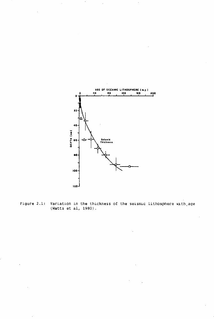
Much a t t e n t i o n has been d i r e c t e d to e s t a b l i s h i n g the thickness of the
seismic l i t h o s p h e r e . Surface wave analyses have demonstrated (Figure 2.1)
th a t the oceanic l i t h o s p h e r e increases i n thickness from 25 km at 5 m i l l i o n
years to 90 km at 100 m i l l i o n years.(Leeds et a l , 1974; Forsyth, 1977).
- 27 -
101 OF OCEANIC LITHOIPHCDC («.».) 00 120 180 too 1 I J •
£0
40
TMe&noao
ao
100
I 1 0 J
Figure 2.1: V a r i a t i o n i n the thickness of the seismic l i t h o s p h e r e w x t h a g e (Watts et a l , 1980).
These observations suggest t h a t the l i t h o s p h e r e increases i n thickness as
i t c o o l s . The c o n t i n e n t a l l i t h o s p h e r e i s g e n e r a l l y t h i c k e r than the
oceanic l i t h o s p h e r e .
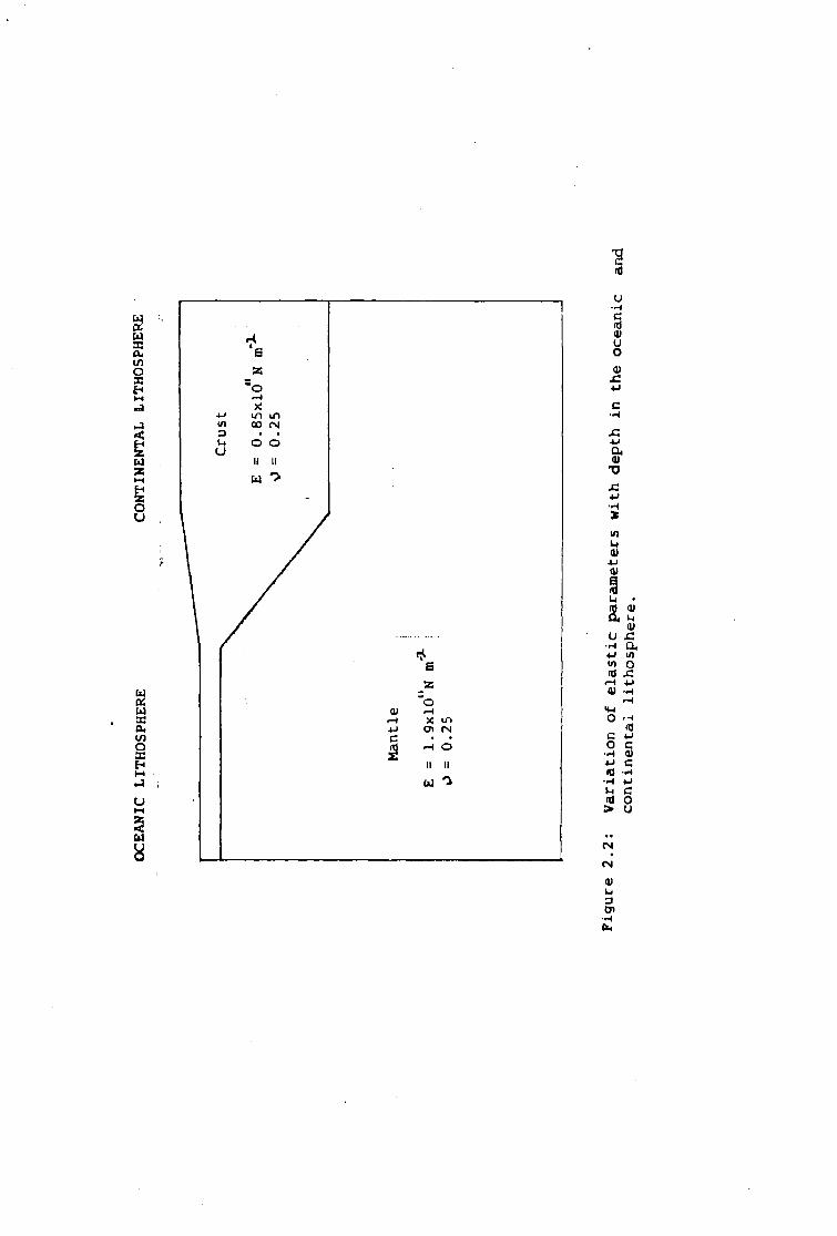
2.3.2 V a r i a t i o n of e l a s t i c parameters w i t h depth
The v e l o c i t y of seismic waves are dependant upon the e l a s t i c
p r o p e r t i e s and d e n s i t y of the medium through which they t r a v e l . The w e l l
known v e l o c i t y and d e n s i t y d i s t r i b u t i o n i n the seismic l i t h o s p h e r e can
consequently be i n v e r t e d t o y i e l d the v a r i a t i o n i n Young's modulus, E, and
Poisson's r a t i o , V, w i t h depth (e.g. Mithen, 1980). This procedure y i e l d s
a d i f f e r e n t p r o f i l e of e l a s t i c parameters i n the c o n t i n e n t a l and oceanic
l i t h o s p h e r e s because of the d i f f e r e n c e s i n t h e i r v e l o c i t y d i s t r i b u t i o n .
The v a r i a t i o n i n the e l a s t i c parameters w i t h depth i n the oceanic and
c o n t i n e n t a l l i t h o s p h e r e which were c a l c u l a t e d by Park (1981) from t h e i r
average v e l o c i t y and d e n s i t y d i s t r i b u t i o n are shown i n f i g u r e 2.2. These
parameters w i l l be used i n subsequent chapters to model the l i t h o s p h e r i c
stress regime.
2.3.3 Non-elastic deformation
Earthquakes are n a t u r a l seismic sources which a r i s e from the
n o n - e l a s t i c deformation of the e a r t h . The r a d i a l d i s t r i b u t i o n of
earthquake f o c i , o u t s i d e of p l a t e c o l l i s i o n zones, i s observed t o be
r e s t r i c t e d t o the upper 10-30 km of the seismic l i t h o s p h e r e ( V e t t e r and
Meissner, 1979). This observation suggests t h a t the l i t h o s p h e r e has a
f i n i t e s t r e n g t h and deforms as a b r i t t l e s o l i d i n the near surface when the
load exceeds the s t r e n g t h of the rocks.
- 23 -
s 41 U
IX 1/1 <U
i n CO (N
U <u i ii
u 0) 01
Li
8, 01 H a, 4-1 l/l in o 0) -H
•4-1 01 <0 0> (N in
II II (0 -H u 1 m o u
(N
01
2.4 Li t h o s p h e r i c Flexure
The l i t h o s p h e r e responds to v e r t i c a l loads, such as those at seamcunts
and deep sea trenches, by bending. The c h a r a c t e r i s t i c f e a t u r e s of t h i s
f l e x u r e are an uparching of the seafloor (known as the outer r i s e a t
trenches and the p e r i p h e r a l bulge at seamounts) some 100-150 km from the
load and a downwards displacement towards i t . This f l e x u r e o r i g i n a t e s a t
seamounts from a s t a t i c v o l c a n i c load, w h i l e at trenches i t r e s u l t s from
the dynamic forces associated w i t h p l a t e convergence. Although the forces
causing f l e x u r e a t trenches and seamounts are d i f f e r e n t the i m p l i c a t i o n s
f o r the the mid to long term rheology of the l i t h o s p h e r e are s i m i l a r .
These i m p l i c a t i o n s are reviewed i n t h i s s e c t i o n .
The l i t h o s p h e r i c f l e x u r e seawards of trenches and seamounts has been
s u c c e s s f u l l y modelled using t h i n e l a s t i c p l a t e theory (Walcott, 1970, 1976 ;
Hanks, 1971; Watts and Talwani, 1974; Watts and Cochran, 1974; Watts et
a l , 1975; Parsons and Molnar, 1976; Caldwell et a l , 1976; Watts, 1978).
This model represents the l i t h o s p h e r e as an e l a s t i c layer and the
asthenosphere as a f l u i d substratum. The two major r e s u l t s which have been
obtained from these models are ( f i g u r e 2.3):
1. The mechanical thickness of the e l a s t i c layer which supports the
load i s between a h a l f or a t h i r d of the seismic thickness of the
l i t h o s p h e r e .
2. The thickness of the e l a s t i c layer increases w i t h age and f o l l o w s
the 300-700°C isotherm of Parsons and Scla t e r (1977).
These r e s u l t s have been i n t e r p r e t e d as demonstrating t h a t the e n t i r e
seismic thickness of the l i t h o s p h e r e does not support long term loads and
t h e r e f o r e t h a t the seismic l i t h o s p h e r e i s d i v i d e d i n t o an e l a s t i c upper
- 29 -
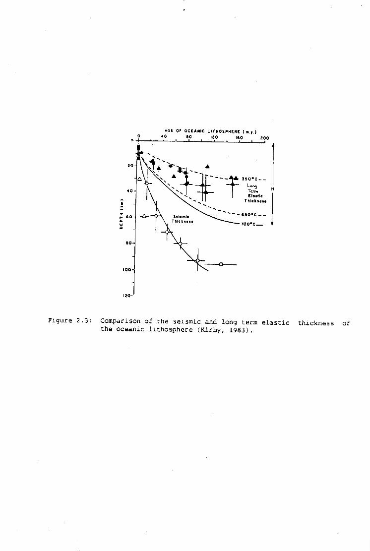
AGE OF OCEANIC LI THOSPHERE I m.j.) 40 80 120 ISO 200 r> -J I I
20
J 5 0 ° C
Lo Tern, 4 0 E la i l l e
Thlckno»«
6 S 0 - C 60-^ - £ * -T h l c t n t a t roo°c
8 0
100
120
Figure 2.3: Comparison of the seismic and long term e l a s t i c thickness of the oceanic l i t h o s p h e r e ( K i r b y , 1983).
layer and a d u c t i l e lower layer whose p o s i t i o n i s t h e r m a l l y c o n t r o l l e d .
Recent models of the topography of these features have shown t h a t
b e t t e r f i t s to p r o f i l e s which have a l a r g e curvature can be obtained using
a rheology which allows some n o n - e l a s t i c deformation to occur i n the
e l a s t i c layer •McAcco et a l , 1978; T u r c o t t e et a l , 1973; 3odine and
Watts, 1979; • Chappie and Forsyth, 1 9 7 9 ) . These models use an
e l a s t i c - p l a s t i c rheolcgy f o r the l i t h o s p h e r e which y i e l d s p l a s t i c a l l y when
the stress i n the e l a s t i c layer exceeds the y i e l d s t r e n g t h of the rocks.
The advantages of t h i s model are t h a t i t produces much more r e a l i s t i c
stresses i n the e l a s t i c layer and i s compatible w i t h the observations of
rock mechanics.
The c o n t i n e n t a l l i t h o s p h e r e , however, has not been subjected to such
exhaustive modelling. This i s because i t i s less homogeneous than the
oceanic l i t h o s p h e r e and because s u i t a b l e loading s t r u c t u r e s do not r e a d i l y
occur. The a v a i l a b l e evidence, however, demonstrates t h a t the c o n t i n e n t a l
l i t h o s p h e r e behaves l i k e the oceanic l i t h o s p h e r e i n t h a t the mechanical
thickness of the e l a s t i c layer i s t h e r m a l l y c o n t r o l l e d and s u b s t a n t i a l l y
t h i n n e r than the seismic thickness (Karner et a l , 1983).
2.5 Rock Mechanics
Rock mechanics can be used to measure the s t r e s s - s t r a i n behaviour of
various l i t h o s p h e r i c c o n s t i t u e n t s at d i f f e r e n t pressures and temperatures
to simulate t h e i r p h y s i c a l behaviour a t depths w i t h i n the e a r t h . Such
experiments provide i n f o r m a t i o n on the p h y s i c a l mechanisms of deformation
w i t h i n the l i t h o s p h e r e and help to e x p l a i n i t s observed time dependent
response to l o a d i n g .
- 30 -
2.5.1 B r i t t l e f r a c t u r e : modified G r i f f i t h theory
The great number of micro- and macro-fractures which are observed i n
c r u s t a l rocks demonstrates t h a t n o n - e l a s t i c deformation occurs near t o the
earths surface. The hypocentres of the earthquakes which occur i n the
upper e l a s t i c l i t h o s p h e r e demonstrates t h a t t h i s b r i t t l e f r a c t u r e extends
to depths of 10-30 km.
These observations are i n agreement w i t h tho known behaviour of
l i t h o s p h e r i c rocks i n l a b o r a t o r y experiments conducted at low temperatures
and pressures. These analyses show t h a t rocks have a f i n i t e s t r e n g t h and
f r a c t u r e when the magnitude of the load exceeds a c r i t i c a l value.
Mathematical d e s c r i p t i o n s of the f a i l u r e of rocks have been proposed
by Coulomb, Mohr and G r i f f i t h s and are reviewed i n Jaeger and Cook (1977).
For reasons discussed i n Mithen (1930), i t i s g e n e r a l l y accepted t h a t a
modified form of the G r i f f i t h f r a c t u r e c r i t e r i o n f i t s best w i t h l a b o r a t o r y
experiments and w i t h the observed f a i l u r e of l i t h o s p h e r i c rocks. This
f a i l u r e c r i t e r i a has been used i n t h i s t h e s i s .
convenient t o describe the modified G r i f f i t h f a i l u r e c r i t e r i a i n
the mean s t r e s s , ^ , and the mean shear s t r e s s , X. , which are
0" + c r » x
2
2
where 0\ and are the maximum and minimum p r i n c i p a l stresses ( w i t h the
convention that tension i s p o s i t i v e ) . The modified G r i f f i t h f a i l u r e
c r i t e r i a can then be defined i n terms of the t e n s i l e s t r e n g t h of the rock, - 31 -
I t i s
terms of
d e f i n e d
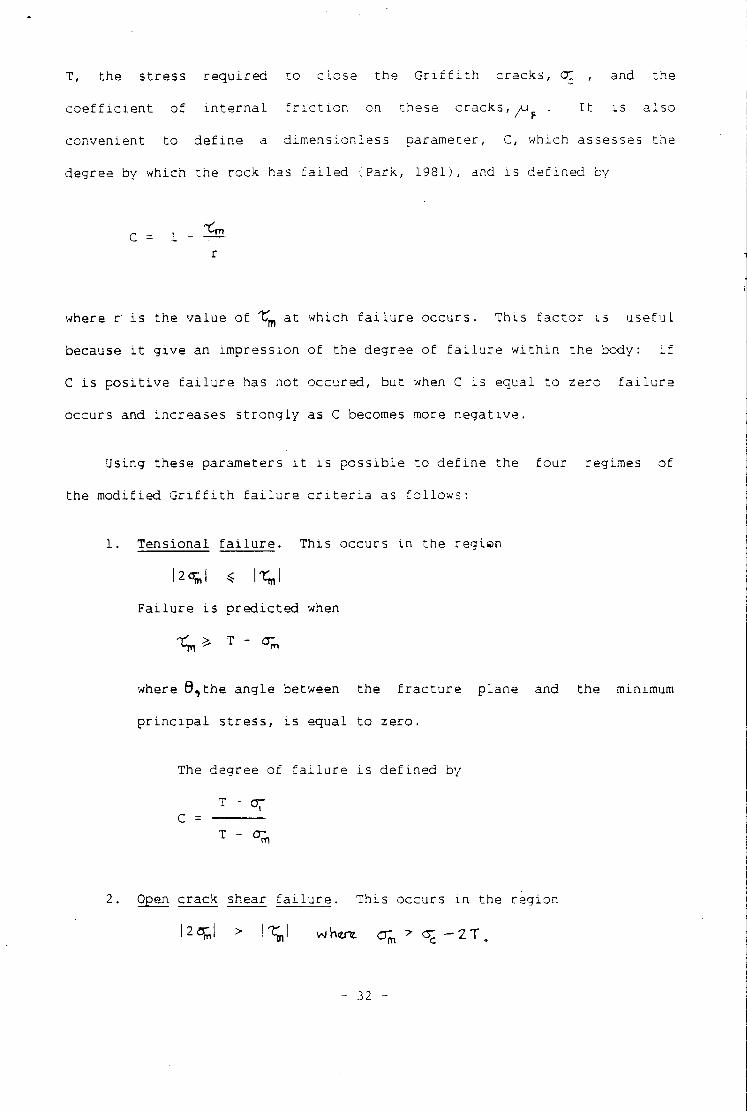
T, the stress r e q u i r e d to close the G r i f f i t h cracks, c£ , and the
c o e f f i c i e n t of i n t e r n a l f r i c t i o n on these cracks,yu . I t i s a l s o
convenient t o d e f i n e a dimensionless parameter, C, which assesses the
degree by which the rock has f a i l e d (Park, 1981), and i s d e f i n e d by
1
where r i s the value of f m at which f a i l u r e occurs. This f a c t o r i s u s e f u l
because i t give an impression of the degree of f a i l u r e w i t h i n the body: i f
C i s p o s i t i v e f a i l u r e has not occured, but when C i s equal t o zero f a i l u r e
occurs and increases s t r o n g l y as C becomes more negative.
Using these parameters i t i s p o s s i b l e to d e f i n e the f o u r regimes of
the modified G r i f f i t h f a i l u r e c r i t e r i a as f o l l o w s :
1. Tensional f a i l u r e • This occurs i n the region
F a i l u r e i s p r e d i c t e d when
where 8,the angle between the f r a c t u r e plane and the minimum
p r i n c i p a l s t r e s s , i s equal t o zero.
The degree of f a i l u r e i s d e f i n e d by
T - 0 7 c =
2. Open crack shear f a i l u r e . This occurs i n the region
|2££,| > 1 w h e n t crm
7 or: - Z T .
- 32 -
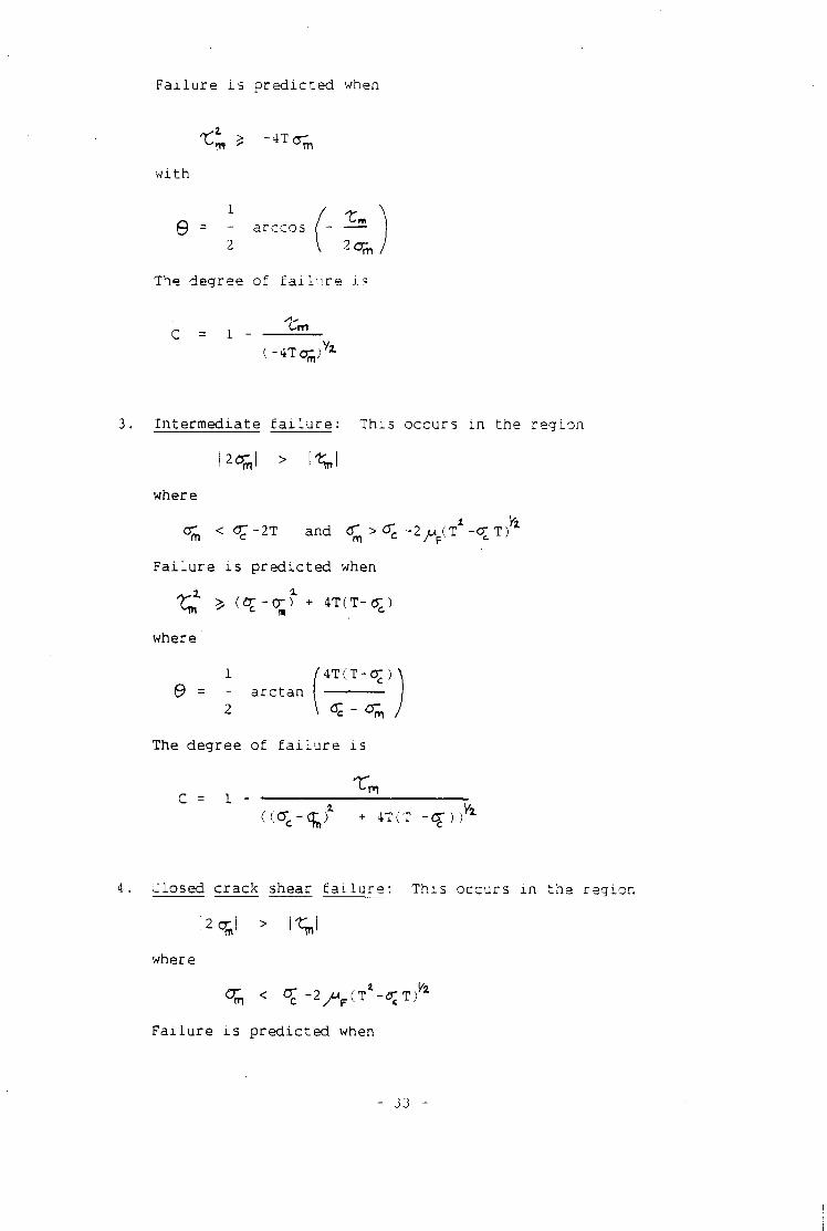
F a i l u r e i s p r e d i c t e d when
< * - 4 T * r n w i t h
1 / X = - arccos ( -
The degree of f a i l u r e i s
C = 1 (-4Tq;) V l
3. Intermediate f a i l u r e : This occurs i n the region
l 2 ^ l > \%\
where
<Tm < 0--2T and <T ><TC -Z^i?* -cr T ) 5 4
F a i l u r e i s p r e d i c t e d when
where
1 /4T(T-Cp\ & = - arctan
2 \ <Z-<rm
The degree of f a i l u r e i s
( ( c r - q ^ ) 1 + 4T(T -Cj ) ) V' 1
4. Closed crack shear f a i l u r e : This occurs i n the region
where
F a i l u r e i s p r e d i c t e d when
- 33 -
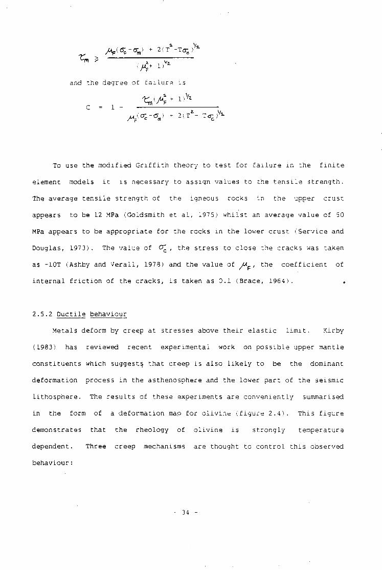
/VCer-cV • 2 ( T 1 - T < 3 - C ) V I -4n 2
and the degree of f a i l u r e i s
C = 1 -^ ( c r - c r ) • 2( T - T«rc)'
To use the modified G r i f f i t h theory to t e s t f o r f a i l u r e i n the f i n i t e
element models i t i s necessary t o assign values to the t e n s i l e s t r e n g t h .
The average t e n s i l e s t r e n g t h of the igneous rocks i n the upper c r u s t
appears to be 12 MPa (Goldsmith et a l , 1975) w h i l s t an average value of 50
MPa appears to be a p p r o p r i a t e f o r the rocks i n the lower c r u s t (Service and
Douglas, 1973). The value of <XC , the stress to close the cracks was taken
as -10T (Ashby and V e r a l l , 1978) and the value of / ^ p / the c o e f f i c i e n t of
i n t e r n a l f r i c t i o n of the cracks, i s taken as 0.1 (Brace, 1964).
2.5.2 D u c t i l e behaviour
Metals deform by creep at stresses above t h e i r e l a s t i c l i m i t . K i rby
(1983) has reviewed recent experimental work on p o s s i b l e upper mantle
c o n s t i t u e n t s which suggests t h a t creep i s also l i k e l y to be the dominant
deformation process i n the asthenosphere and the lower p a r t of the seismic
l i t h o s p h e r e . The r e s u l t s of these experiments are c o n v e n i e n t l y summarised
i n the form of a deformation map f o r o l i v i n e ( f i g u r e 2.4). This f i g u r e
demonstrates that the rheology of o l i v i n e i s s t r o n g l y temperature
dependent. Three creep mechanisms are thought to c o n t r o l t h i s observed
behaviour:
- 34 -
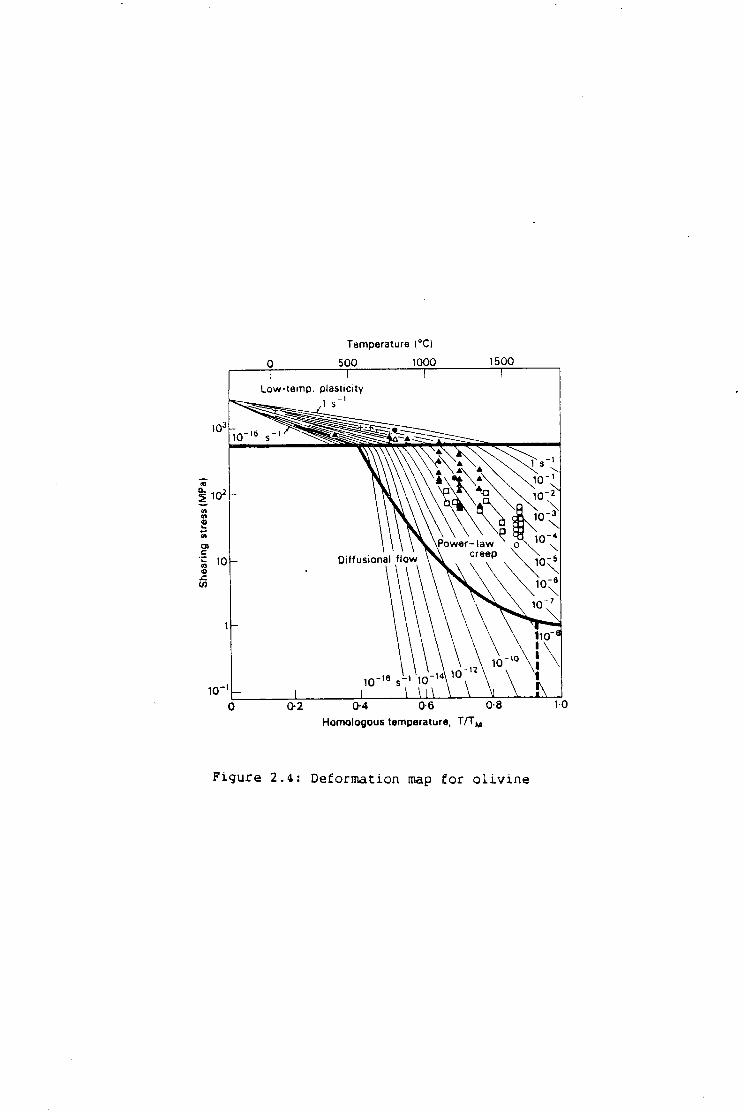
Temperature ( C)
1500 1000 500
Low-temp, plasticity
1 s
103
10
5 102
(A 10 en
\ (A 10 Power- law creep Diffusional flow 10 <0
a 10
10 \ 1 no \ I \ I 10 0 I 12
\ I 18 ' 10 10 10
10 0-8 0-6 0-4 0-2 Homologous temperature, T/T
Figure 2.4: Deformation map f o r o l i v i n e
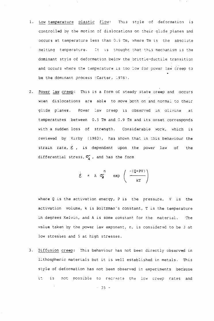
Low temperature p l a s t i c f l o w : This s t y l e of deformation i s
c o n t r o l l e d by the motion of d i s l o c a t i o n s on t h e i r g l i d e planes and
occurs at temperature less than 0.5 Tm, where Tm i s the absolute
m e l t i n g temperature. I t i s thought t h a t t h i s mechanism i s the
dominant s t y l e of deformation below the b r i t t l e - d u c t i l e t r a n s i t i o n
and occurs where the temperature i s too low f o r power law creep to
be the dominant process ( C a r t e r , 1976).
Power law creep: This i s a form of steady s t a t e creep and occurs
when d i s l o c a t i o n s are able to move both on and normal to t h e i r
g l i d e planes. Power law creep i s observed i n o l i v i n e at
temperatures between 0.5 Tm and 0.9 Tm and i t s onset corresponds
w i t h a sudden loss of s t r e n g t h . Considerable work, which i s
reviewed by Ki r b y (1983), has shown t h a t i n t h i s behaviour the
s t r a i n r a t e , £ , i s dependent upon the power law of the
d i f f e r e n t i a l s t r e s s , OT , and has the form
where Q i s the a c t i v a t i o n energy, P i s the pressure, V i s the
a c t i v a t i o n volume, k i s Boltzman's constant, T i s the temperature
i n degrees K e l v i n , and A i s some constant f o r the m a t e r i a l . The
value taken by the power law exponent, n, i s considered to be 3 at
low stresses and 5 a t high stresses.
D i f f u s i o n creep: This behaviour has not been d i r e c t l y observed i n
l i t h o s p h e r i c m a t e r i a l s but i t i s w e l l e s t a b l i s h e d i n metals. This
s t y l e of deformation has not been observed i n experiments because
i t i s not pos s i b l e to recreate the low creep rates and
n (Q+PV) exp
kT
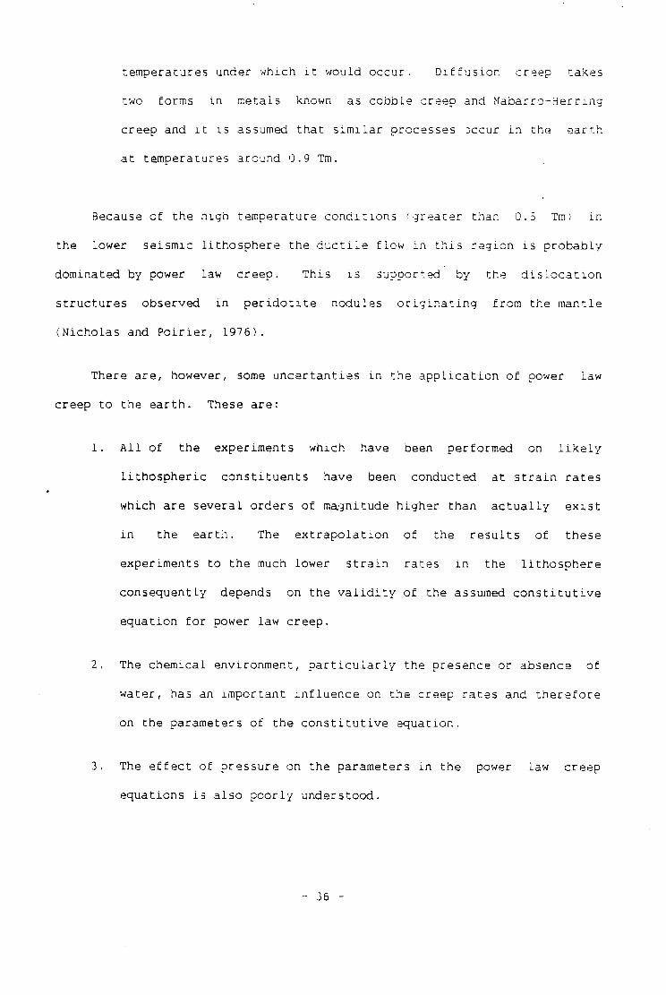
temperatures under which i t would occur. D i f f u s i o n creep takes
two forms i n metals known as cobble creep and Nabarro-Herrmg
creep and i t i s assumed t h a t s i m i l a r processes occur i n the ea r t h
at temperatures around 0.9 Tm.
Because of the high temperature c o n d i t i o n s f g r e a t e r than 0.5 Tm) i n
the lower seismic l i t h o s p h e r e the d u c t i l e flow i n t h i s region i s probably
dominated by power law creep. This i s supported by the d i s l o c a t i o n
s t r u c t u r e s observed i n p e r i d o t i t e nodules o r i g i n a t i n g from the mantle
(Nicholas and P o i r i e r , 1976).
There are, however, some u n c e r t a n t i e s i n the a p p l i c a t i o n of power law
creep t o the e a r t h . These are:
1. A l l of the experiments which have been performed on l i k e l y
l i t h o s p h e r i c c o n s t i t u e n t s have been conducted at s t r a i n r a t e s
which are several orders of magnitude higher than a c t u a l l y e x i s t
i n the ea r t h . The e x t r a p o l a t i o n of the r e s u l t s of these
experiments to the much lower s t r a i n rates i n the l i t h o s p h e r e
consequently depends on the v a l i d i t y of the assumed c o n s t i t u t i v e
equation f o r power law creep.
2. The chemical environment, p a r t i c u l a r l y the presence or absence of
water, has an important i n f l u e n c e on the creep rates and t h e r e f o r e
on the parameters of the c o n s t i t u t i v e equation.
3. The e f f e c t of pressure on the parameters i n the power law creep
equations i s also p o o r l y understood.
- 36 -
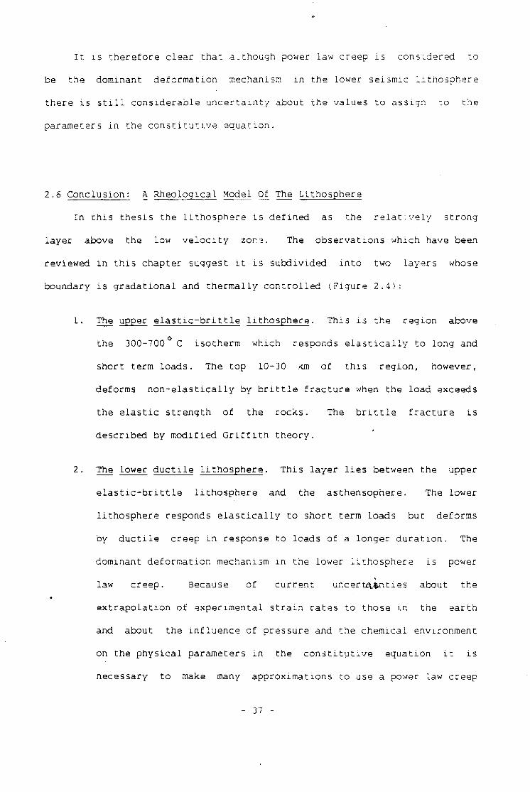
I t i s t h e r e f o r e c l e a r t h a t a.though power law creep i s considered t o
be the dominant deformation mechanism i n the lower seismic l i t h o s p h e r e
there i s s t i l l considerable u n c e r t a i n t y about the values t o assign to the
parameters i n the c o n s t i t u t i v e equation.
2.6 Conclusion: A Rheological Model Of The Lithosphere
In t h i s t h e s i s the l i t h o s p h e r e i s d e f i n e d as the r e l a t i v e l y strong
layer above the low v e l o c i t y zor3. The observations which have been
reviewed i n t h i s chapter suggest i t i s subdivided i n t o two layers whose
boundary i s g r a d a t i o n a l and t h e r m a l l y c o n t r o l l e d (Figure 2 . 4 ) :
1. The upper e l a s t i c - b r i t t l e l i t h o s p h e r e . This i s the region above
the 300-700° C isotherm which responds e l a s t i c a l l y t o long and
short term loads. The top 10-30 km of t h i s r e g i o n , however,
deforms n o n - e l a s t i c a l l y by b r i t t l e f r a c t u r e when the load exceeds
the e l a s t i c s t r e n g t h of the rocks. The b r i t t l e f r a c t u r e i s
described by modified G r i f f i t h theory.
2. The lower d u c t i l e l i t h o s p h e r e . This l a y e r l i e s between the upper
e l a s t i c - b r i t t l e l i t h o s p h e r e and the asthensophere. The lower
l i t h o s p h e r e responds e l a s t i c a l l y t o short term loads but deforms
by d u c t i l e creep i n response to loads of a longer d u r a t i o n . The
dominant deformation mechanism i n the lower l i t h o s p h e r e i s power
law creep. Because of c u r r e n t u n c e r t a i n t i e s about the
e x t r a p o l a t i o n of experimental s t r a i n r ates t o those i n the ea r t h
and about the i n f l u e n c e of pressure and the chemical environment
on the p h y s i c a l parameters i n the c o n s t i t u t i v e equation i t i s
necessary to make many approximations to use a power law creep
- 37 -
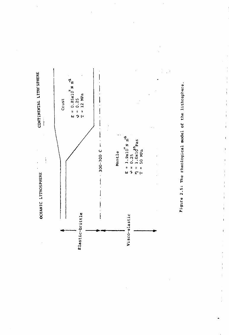
u X CL 1/1 t_ X E-t
•J
U
o u
w « a. tn o x H
u t-H
u 8
O
•a
"o r-l rO ui if) J oo (N • • (N
O O r-t
II II II
U "> t-i
u o o r-i o o m
•a 2 "o
in rd a.
c rd
<J> fN O • • . o
h o m II II
w o ii ii
C E-t
I u in
«
u •w 4-1
rd r - t 01 I o (J 1/1
>
a in O J5
0)
0 .-i
rd U
o o tu x: u at c ft in <N
<U u 3 Co
rheology t o model deformation i n the lower l i t h o s p h e r e . An
a l t e r n a t i v e and simpler approach i s to use a Maxwell v i s c o - e l a s t i c
rheology to model deformation i n t h i s l a y e r . Recent studies
(Mithen, 1980; Melosh and Raefsky, 1980) have demonstrated t h a t
the f i n a l s t r e s s regime using e i t h e r power law creep or a 23
v i s c o - e l a s t i c rheology w i t h a v i s c o s i t y of 1.0x10 Pa s are almost
i d e n t i c a l . The major d i f f e r e n c e between these two deformation
mechanisms i s that higher d e v i a t o r i c stresses i n i t i a l l y r e l a x
f a s t e r i n a power law creep m a t e r i a l . The deformation p r e d i c t e d
by these two r h e o l o g i c a l models, however, converges once
e q u i l i b r i u m i s reached and both mechanisms produce stress
c o n c e n t r a t i o n i n the upper e l a s t i c l i t h o s p h e r e ( 3 o t t and Kusznir,
1979; Mithen, 1980). In t h i s t h e s i s the deformation of t h i s
l ayer w i l l consequently be modelled by a v i s c o - e l a s t i c substance
w i t h a v i s c o s i t y of 1.0x10 Pa s. I t i s important, however, t o
appreciate t h a t t h i s i s j u s t a convenient s i m p l i f i c a t i o n t o model
the stress regime at subduction zones.
This model i s summarised i n f i g u r e 2.5.
- 33 -
CHAPTER 3
THE ISOPARAMETRIC FINITE ELEMENT METHOD
3.1 I n t r o d u c t i o n
To o b t a i n r e a l i s t i c models of the stress regime at subduction zones i t
i s necessary to use a s o l u t i o n technique which i s capable of g i v i n g
accurate and p r e d i c t i v e aaswers t o problems i n v o l v i n g :
1. Flexure of the l i t h o s p h e r e .
2. Bodies w i t h various m a t e r i a l types.
3. Bodies w i t h complex geometries.
4. Complex boundary c o n d i t i o n s .
5. The curved d i s c o n t i n u i t y of the subduction zone f a u l t .
6. E l a s t i c and time dependent r h e o l o g i e s .
A n a l y t i c s o l u t i o n s to problems of t h i s complexity are i m p r a c t i c a b l e . I t i s
t h e r e f o r e d e s i r a b l e t o use d i g i t a l computers t o o b t a i n approximate
s o l u t i o n s using numerical mathematical techniques. One numerical method
which has been e x t e n s i v e l y and s u c c e s s f u l l y used i n stress a n a l y s i s i s the
f i n i t e element method. This technique w i l l consequently be used i n t h i s
t h e s i s t o model l i t h o s p h e r i c stress regimes.
The f i r s t step i n the f i n i t e element method i s to d i v i d e the body i n t o
a number of f i n i t e elements which interconnect a t a series of nodes.
Assumptions are then made about the behaviour of the major v a r i a b l e s w i t h i n
each element. The main assumption i s the choice of the order of the
displacement f u n c t i o n , which defines the v a r i a t i o n of the displacements
w i t h i n each element. Once t h i s f u n c t i o n has been chosen i t i s p o s s i b l e t o
- 39 -
express the displacement of a general p o i n t w i t h i n an element as an
i n t e r p o l a t i o n of i t s known nodal values. Expressions can then be obtained
f o r the stress and s t r a i n at a general p o i n t w i t h i n an element so t h a t , by
con s i d e r i n g the energy of the system, an e q u i l i b r i u m equation can be
derive d which r e l a t e s the displacement and the a p p l i e d forces at the nodes
to the s t i f f n e s s of the body.
The f i n i t e elements used by previous researchers at Durham (Dean,
1973; Kusznir, 1976; Woodward, 1976; Mithen, 1980; Park, 1981; L i n t o n ,
1982) were based upon a l i n e a r displacement f u n c t i o n . This r e s u l t s i n a
constant s t r a i n w i t h i n each element. This i s the simplest of the two
dimensional f i n i t e elements and i t s major advantage i s that i t allows an
e x p l i c i t expression t o be d e r i v e d f o r the s t i f f n e s s of the body. For
reasons discussed i n Chapter 4, however, t h i s element does not perform w e l l
i n many e l a s t i c and v i s c o - e l a s t i c problems where the s t r a i n g r a d i e n t i s
h i gh.
Because of these l i m i t a t i o n s a higher order f i n i t e element, which i s
based upon a q u a d r a t i c displacement f u n c t i o n , i s used i n t h i s t h e s i s .
Since the s t r a i n v a r i e s l i n e a r l y w i t h i n these elements they should perform
b e t t e r i n regions w i t h a high s t r a i n g r a d i e n t .
The simplest two dimensional f i n i t e element which i s based upon a
quadratic displacement f u n c t i o n i s the plane sided t r i a n g u l a r element
(F e l i p p a , 1966; Desai and Abel, 1972). The advantage of t h i s element i s
t h a t an e x p l i c i t expression can be obtained f o r the s t i f f n e s s of the body
by using a s p e c i a l l o c a l co-ordinate system. This approach provides a
simple t r a n s i t i o n between the l i n e a r c-.nd q u a d r a t i c displacement f u n c t i o n
methods but i t cannot be used to introduce curved sided elements.
- 40 -
Another technique which i s based upon a q u a d r a t i c displacement
f u n c t i o n i s the isoparametric f i n i t e element method ( Z i e n k i e w i c z , 1977;
Cook, 1981). This method allows curved sided f i n i t e elements to be
introduced, and consequently, i t i s used i n t h i s t h e s i s to model
l i t h o s p h e r i c stress regimes.
In t h i s chapter the theory of the isoparametric method i n e l a s t i c and
v i s c o - e l a s t i c problems i s given f o r both t r i a n g u l a r and q u a d r i l a t e r a l
f i n i t e elements. A computer program (I50FELP) which i s based upon t h i s
technique i s described i n the Appendix.
3.2 The Local Co-ordinate System
When curved sided isoparametric f i n i t e elements are being used i t i s
convenient t o perform the necessary mathematical operations i n a simple
l o c a l co-ordinate system.
3.2.1 Local co-ordinate system f o r t r i a n g u l a r elements
The t r i a n g u l a r element which w i l l be used i n t h i s t h e s i s has a t o t a l
of s i x nodes, three of which l i e a t the v e r t i c e s and three at the midpoints
of the sides of the t r i a n g l e . The nodes of the element are numbered
clockwise or a n t i c l o c k w i s e around the element s t a r t i n g w i t h one of the
nodes at an apex. Figure 3.1 i l l u s t r a t e s "the geometry of t h i s element and
f i g u r e 3.2 shows how the g l o b a l element geometry i s mapped onto the l o c a l
( s , t ) space. I t can be seen t h a t the curved sides of the element i n g l o b a l
co-ordinates are transformed t o s t r a i g h t sided sections of u n i t l e n g t h i n
the l o c a l reference system, which has i t s o r i g i n at node 1.
- 41 -
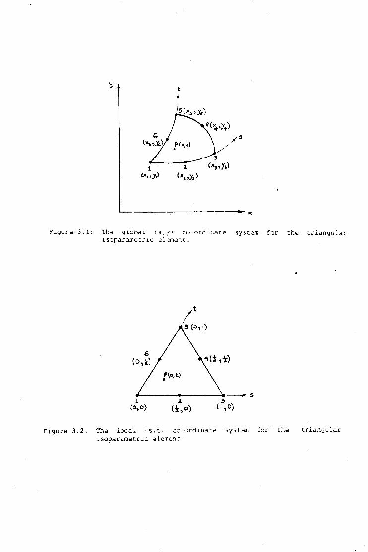
F i g u r e 3.1 The g l o b a l x,y; c o - o r d i n a t e system f o r t h e t r i a n g u l a i s o p a r a m e t r i c element
a (o, i)
1 (1,0)
F i g u r e 3.2: The l o c a l (s,t.> c o - o r d i n a t e system f o r t h e t r i a n g u l a r i s o p a r a m e t r i c element.
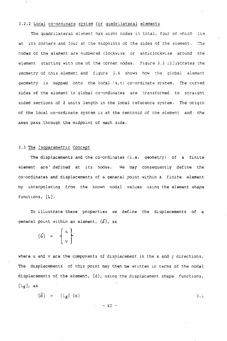
3.2.2 L o c a l c o - o r d i n a t e systam f o r q u a d r i l a t e r a l elements
The q u a d r i l a t e r a l element has e i g h t nodes i n t o t a l , f o u r o f w h i c h l i e
a t i t s c o r n e r s and f o u r a t t h e m i d p o i n t s o f t h e s i d e s o f t h e e l e m e n t . The
nodes o f t h e element a r e numbered c l o c k w i s e o r a n t i c l o c k w i s e around t h e
element s t a r t i n g w i t h one o f t h e c o r n e r nodes. F i g u r e 3.3 i l l u s t r a t e s t h e
geometry o f t h i s element and f i g u r e 3.4 shows how t h e g l o b a l element
geometry i s mapped o n t o t h e l o c a l ( s , t ) c o - o r d i n a t e system. The c u r v e d
s i d e s o f t h e element i n g l o b a l c o - o r d i n a t e s a r e t r a n s f o r m e d t o s t r a i g h t
s i d e d s e c t i o n s o f 2 u n i t s l e n g t h i n t h e l o c a l r e f e r e n c e system. The o r i g i n
o f t h e l o c a l c o - o r d i n a t e system i s a t t h e c e n t r o i d o f t h e element and t h e
axes pass t h r o u g h t h e m i d p o i n t o f each s i d e .
3.3 The I s o p a r a m e t r i c Concept
The d i s p l a c e m e n t s and t h e c o - o r d i n a t e s ( i . e . geometry) o f a f i n i t e
element a r e " d e f i n e d a t i t s nodes. We may c o n s e q u e n t l y d e f i n e t h e
c o - o r d i n a t e s and d i s p l a c e m e n t s o f a g e n e r a l p o i n t w i t h i n a f i n i t e element
by i n t e r p o l a t i n g f r o m t h e known n o d a l v a l u e s u s i n g t h e element shape
f u n c t i o n s , [ L ] .
To i l l u s t r a t e t h e s e p r o p e r t i e s we d e f i n e t h e d i s p l a c e m e n t s o f a
g e n e r a l p o i n t w i t h i n an e l e m e n t , (<£"}, as
u
v
where u and v a r e t h e components o f d i s p l a c e m e n t i n t h e x and y d i r e c t i o n s .
The d i s p l a c e m e n t s o f t h i s p o i n t may t h e n be w r i t t e n i n terms o f t h e n o d a l
d i s p l a c e m e n t s o f t h e element, { d } , u s i n g t h e - d i s p l a c e m e n t shape f u n c t i o n s ,
[ L j ] , as
(£} = [Lg] i d } 3.1
- 42 -
3 i
F i g u r e 3.3: The g l o b a l <x,y> c o - o r d i n a t e system f o r t h e q u a d r i l a t e r a l i s o p a r a m e t r i c f i n i t e e l e m e n t .
(-1,0)
i
6(0.0 ^ ( • i 0 • * ^ ( • i 0
1 * © p
(«,0 •- ( »3f l .-ft
f-i»-0 (0,-1) F i g u r e 3.4: The l o c a l ( s , t > c o - o r d i n a t e system f o r t h e q u a d r i l a t e r a l
i s o p a r a m e t r i c f i n i t e e l ement.
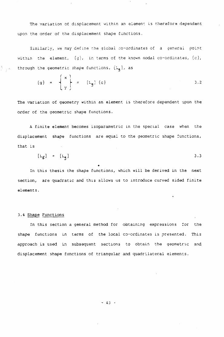
The v a r i a t i o n o f d i s p l a c e m e n t w i t h i n an element i s t h e r e f o r e dependent
upon t h e o r d e r o f t h e d i s p l a c e m e n t shape f u n c t i o n s .
S i m i l a r l y , we may d e f i n e t h e g l o b a l c o - o r d i n a t e s of a g e n e r a l p o i n t
w i t h i n t h e element, ( g ) , i n terms o f t h e known n o d a l c o - o r d i n a t e s , f c } ,
t h r o u g h t h e g e o m e t r i c shape f u n c t i o n s , [ L ^ ] , as
r x 1
Cg} = -I I- = [L ] { c } 3.2 I Y J 3
The v a r i a t i o n o f geometry w i t h i n an element i s t h e r e f o r e dependent upon t h e
o r d e r o f t h e g e o m e t r i c shape f u n c t i o n s .
A f i n i t e element becomes i s o p a r a m e t r i c i n t h e s p e c i a l case when t h e
d i s p l a c e m e n t shape f u n c t i o n s a r e e q u a l t o t h e g e o m e t r i c shape f u n c t i o n s ,
t h a t i s
[LS] = [ L a J 3.3
I n t h i s t h e s i s t h e shape f u n c t i o n s , w h i c h w i l l be d e r i v e d i n t h e n e x t
s e c t i o n , a r e q u a d r a t i c and t h i s a l l o w s us t o i n t r o d u c e c u r v e d s i d e d f i n i t e
element s.
3.4 Shape F u n c t i o n s
I n t h i s s e c t i o n a g e n e r a l method f o r
shape f u n c t i o n s i n terms o f t h e l o c a l
a p p r o a c h i s used i n subsequent s e c t i o n s
d i s p l a c e m e n t shape f u n c t i o n s o f t r i a n g u l a r
o b t a i n i n g e x p r e s s i o n s f o r t h e
c o - o r d i n a t e s i s p r e s e n t e d . T h i s
t o o b t a i n t h e g e o m e t r i c and
and q u a d r i l a t e r a l e l e m e n t s .
- 43 -
3.4.1 G e n e r al d e f i n i t i o n and e v a l u a t i o n o f shape f u n c t i o n s
Shape f u n c t i o n s , N^, d e f i n e t h e v a l u e o f an a r b i t r a r y f u n c t i o n , f , az
any p o i n t w i t h i n an element t h r o u g h an i n t e r p o l a t i o n o f t h e known n o d a l
v a l u e s , f n , o f t h e f u n c t i o n .
We may d e f i n e t h e shape f u n c t i o n s N ^ S j t ) , N z ( s , t ) , , N ( 5 , t ) , o f
an m-noded f i n i t e element w i t h n o d a l v a l u e s f, , f , f m , o f t h e
f u n c t i o n f such t h a t i t s v a l u e a t a g e n e r a l p o i n t , f ( s , t ) , w i t h i n , t h e
element i s g i v e n by
f ( s , t ) = N k ( s , t ) f , + N 2 ( s , t ) f 2 + + N m ( s , t ) f m 3.4
We must a l s o choose t h e shape f u n c t i o n s f o r t h e i - t h node such t h a t
f ( s ^ t ^ ) = f j _ , and t h e r e f o r e we d e f i n e
N . ( s L , t c ) = 1
N ^ ( s - , t j ) - 0 i i j
E x p r e s s i o n s f o r t h e shape f u n c t i o n s can be o b t a i n e d by d e f i n i n g t h e
way i n which t h e f u n c t i o n f v a r i e s w i t h i n an e l e m e n t . The most g e n e r a l
r e p r e s e n t a t i o n i s by a p o l y n o m i a l chosen such t h a t
f ( s , t ) = a, + a 2 s + a 3 t + + at n
s' V t' V 3 - 5
where t h e c o e f f i c i e n t s o f t h e p o l y n o m i a l , a- , a r e c o n s t a n t f o r any e l e m e n t .
E q u a t i o n 3.5 can be r e w r i t t e n i n m a t r i x form as
f = [Q] ( a } 3.6
where
[Qj = [ 1 s t s 1.... s * t v ]
and
T f a ) = f a a a, a }
- 44 -
We now seek t o s o l v e e q u a t i o n 3.6 f o r t h e unknown c o n s t a n t s [ a } .
E x a m i n a t i o n o f e q u a t i o n 3.6 d e m o n s t r a t e s t h a t t h e v a l u e t a k e n by t h e
f u n c t i o n f i s dependent upon p o s i t i o n i n t h e element, and t h e r e f o r e ,
because t h e p o s i t i o n o f t h e nodes a r e known i t i s p o s s i b l e t o use t h i s
e q u a t i o n t o o b t a i n e x p r e s s i o n s f o r t h e n o d a l v a l u e s o f the f u n c t i o n f .
f, ( s , , t . )
f z f s z , t 2 )
f (s„,t m) = m m' trv a, + a s_ + a , t + . y "v + a _ t _ s _ .
These n o d a l v a l u e s , ( f n ) , o f t h e f u n c t i o n f can be w r i t t e n i n m a t r i x
f o r m as
where
{ f n } = [A] { a }
[A ]
1 s, t ,
1 st tz
1 s_ t _
3.7
We can t h e r e f o r e o b t a i n e x p r e s s i o n s f o r t h e c o e f f i c i e n t s , { a } , by
i n v e r t i n g e q u a t i o n 3.7. T h i s g i v e s
{a} = [A ] Cf„} 3.8
An e x p r e s s i o n f o r t h e v a l u e o f t h e f u n c t i o n f a t a g e n e r a l p o i n t can
now be o b t a i n e d by s u b s t i t u t i n g t h e above a q u a t i o n i n t o e q u a t i o n 3.6,
g i v i n g
f = [Q] [ A ] { f h } 3.9
R e c a l l i n g e q u a t i o n 3.4, we a r e s e e k i n g shape f u n c t i o n s , such t h a t
N,f, + N t f z •
45
w h i c h may be w r i t t e n i n m a t r i x form as
f = [N] Ce h) 3.10
where
[N] = [ M, N 3 N m ]
Comparing e q u a t i o n s 3.9 and 3.10 we may w r i t e t h e shape f u n c t i o n s as
- 1 [N] • [ 1 ] [ A ] 3..U
We can t h e r e f o r e o b t a i n e x p r e s s i o n s f o r t h e shape f u n c t i o n s i f we can
o b t a i n an i n v e r s e o f t h e m a t r i x [ A ] .
3.4.2 Shape f u n c t i o n s o f a t r i a n g u l a r element
We now proceed t o e v a l u a t e t h e shape f u n c t i o n s f o r a s i x noded
t r i a n g u l a r i s o p a r a m e t r i c f i n i t e e l e m e n t .
3.4.3 Di s p l a c e m e n t shape f u n c t i o n s
The d i s p l a c e m e n t shape f u n c t i o n s can be e v a l u a t e d by d e f i n i n g t h e way
i n w h i c h t h e d i s p l a c e m e n t s v a r y w i t h i n t h e el e m e n t . I n t h i s t h e s i s a
q u a d r a t i c d i s p l a c e m e n t f u n c t i o n has been chosen and we may t h e r e f o r e
express t h e components o f t h e d i s p l a c e m e n t s o f a g e n e r a l p o i n t , u s i n g t h e
q u a d r a t i c f o r m o f t h e p o l y n o m i a l ( e q u a t i o n 3 .5), as
u ( s , t ) = a ( + a^s + a 3 t + a.. s l + a 5 t * + a f a s t 3.12
v ( s , t ) = b, + b s + b t + bi s 2 + b - 1 2 + b, s t ' 2*. 3 ^ ^ k
where t h e u component o f d i s p l a c e m e n t may be w r i t t e n i n m a t r i x f o r m as
u = [Q] ( a } 3.13
i n w h i c h
and
[Q] = [ 1 s t s1" t 1 s t ]
T (a} = ( a , az a^ a^ a 5 aQ }
- 46 -
S i n c e t h e d i s p l a c e m e n t i s a f u n c t i o n o f p o s i t i o n w i t h i n t h e element
and t h e l o c a l c o - o r d i n a t e o f each node i s known ( f i g u r e 3.1) we can
e v a l u a t e e q u a t i o n 3.12 a t each node, g i v i n g
u,( 0 , 0 ) - a,
1 1 u ( - , 0 )
2 ( 4 a , + 2a + a^ )
u ? ( 1 , 0 )
u<( 1 1
2 2
a, + a 1 + a 4
(4a, + 2a, + 2a„ + a^ + a_ + a, ) l 2. ^ <?• 5 fc.
u 5 ( 0 , 1 )
U f( 0 , - ) 2
(4a + 2 a ? + a s )
whi c h may be w r i t t e n i n m a t r i x f o r m as
( u n } = [ A ] { a }
where
[A]
0
2
4
2
0
0
0
0
0
2
4
2
0 0
0 0
0 4
0
1
0
0
3.14
and
C u t u. u 3 u ^ u ^
We can o b t a i n e x p r e s s i o n s f o r t h e c o e f f i c i e n t s , ( a } , by i n v e r t i n g
e q u a t i o n 3.14, wh i c h g i v e s
- 1 { a } = [A] ( u n ) 3.15
- 47
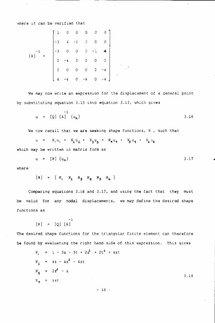
where i t can be v e r i f i e d t h a t
- 1 [ A ]
1 0 0 0 0 0
-3 4 -1 0 0 0
-3 0 0 0 - 1 4 2 -4 2 0 0 0
2 0 0 0 2 -4
4 -4 0 -4 0 -4
We may now w r i t e an e x p r e s s i o n f o r t h e d i s p l a c e m e n t o f a g e n e r a l p o i n t
by s u b s t i t u t i n g e q u a t i o n 3.15 i n t o e q u a t i o n 3.13, which g i v e s
- 1 [Q] [ A ] ( u j 3.16
We now r e c a l l t h a t we a r e s e e k i n g shape f u n c t i o n s , N , such t h a t
u = N,u, + bf 1u 2_ + N 3 u 3 + N^u 4 + N 5 u s + N bu f c
w h i c h may be w r i t t e n i n m a t r i x f o r m as
u = [N] { u n } 3.17
where
[N] = [ N, N 2 N 5 N s Nfe ]
Comparing e q u a t i o n s 3.16 and 3.17, and u s i n g t h e f a c t t h a t t h e y must
be v a l i d f o r any n o d a l d i s p l a c e m e n t s , we may d e f i n e t h e d e s i r e d shape
f u n c t i o n s as
- 1 [N] = [Q] [ A ]
The d e s i r e d shape f u n c t i o n s f o r t h e t r i a n g u l a r f i n i t e element can t h e r e f o r e
be f o u n d by e v a l u a t i n g t h e r i g h t hand s i d e o f t h i s e x p r e s s i o n . T h i s g i v e s
M, = 1 - 3s - 3 t + 2sL + 2tx + 4 s t
N„ = 4s - 4 s 2 - 4 s t
N 5 = 2s 2 - s
= 4st 3.18
43
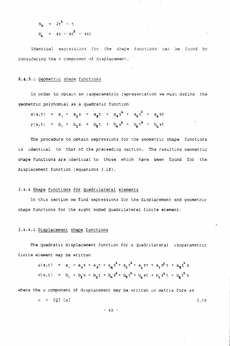
N 5 = 2 t * - t
2 N, = 4t - 4 t - 4 s t 6
I d e n t i c a l e x p r e s s i o n s f o r t h e shape f u n c t i o n s can be fou n d by
c o n s i d e r i n g t h e v component o f d i s p l a c e m e n t .
3 . 4.3.1 Geomet r i c shape f u n c t i o n s
I n o r d e r t o o b t a i n an i s o p a r a m e t r i c r e p r e s e n t a t i o n we must d e f i n e t h e
g e o m e t r i c p o l y n o m i a l as a q u a d r a t i c f u n c t i o n X i
x ( s , t ) = a, + a^s + a 3 t + a 4 s + a $ t + a ^ s t
y ( s , t ) = b, + bLs + b 3 t + b^ s z + b ? t 1 + b f c s t
The p r o c e d u r e t o o b t a i n e x p r e s s i o n s f o r t h e g e o m e t r i c shape f u n c t i o n s
i s i d e n t i c a l t o t h a t o f t h e p r e c e e d i n g s e c t i o n . The r e s u l t i n g g e o m e t r i c
shape f u n c t i o n s a r e i d e n t i c a l t o t h o s e w h i c h have been f o u n d f o r t h e
d i s p l a c e m e n t f u n c t i o n ( e q u a t i o n s 3.18).
3.4.4 Shape f u n c t i o n s f o r q u a d r i l a t e r a l elements
I n t h i s s e c t i o n we f i n d e x p r e s s i o n s f o r t h e d i s p l a c e m e n t and g e o m e t r i c
shape f u n c t i o n s f o r t h e e i g h t noded q u a d r i l a t e r a l f i n i t e e l e m e n t .
3.4.4.1 D i s p l a c e m e n t shape f u n c t i o n s
The q u a d r a t i c d i s p l a c e m e n t f u n c t i o n f o r a q u a d r i l a t e r a l i s o p a r a m e t r i c
f i n i t e element may be w r i t t e n
u ( s , t ) = a, + a s + a , t +• a s 1 * a t Z + a, s t + a s z t + a . t ^ s I 2. 3 4- 3 b 7 B
v ( s , t ) = b, + b 2 s + b 3 t + b ^ s a + bg t 2 " * b ^ s t + b s l t + b^tS
where t h e u component o f d i s p l a c e m e n t may be w r i t t e n i n m a t r i x f o r m as
u = [Q] ( a } 3.19
- 49 -
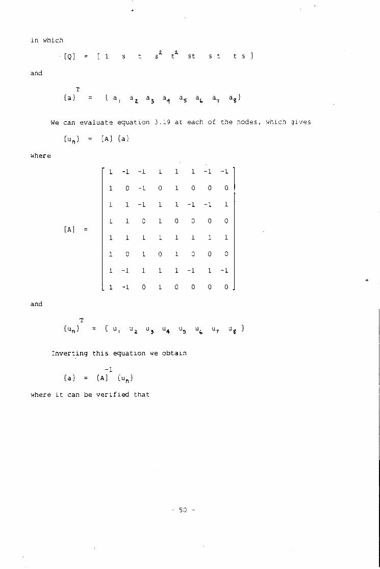
i n w hich
[Q] = [ 1 S t 5 Z t 1 St S t t S
and
( a ) C a i at a 3 a 1 aS afc a7 a S }
We can e v a l u a t e e q u a t i o n 3.19 a t each o f t h e nodes, which g i v e s
Cu n} = [ A ] { a }
where
[A]
1 - 1
1 0
1 - 1
1 - 1
1
0
1
1
1 1
0
1
1
1 1 - 1 - 1
1 0 0 0
1 - 1 - 1 1
0 0
1
1 0
1 - 1
0 0
0 0
1 1
0 0
1 - 1
0 0
and
Cu h} C u, u 2 u 3 u 4 u 5 u f c u 7 u% }
I n v e r t i n g t h i s e q u a t i o n we o b t a i n
( a ) = [ A ] ( u n )
where i t can be v e r i f i e d t h a t
- 50 -
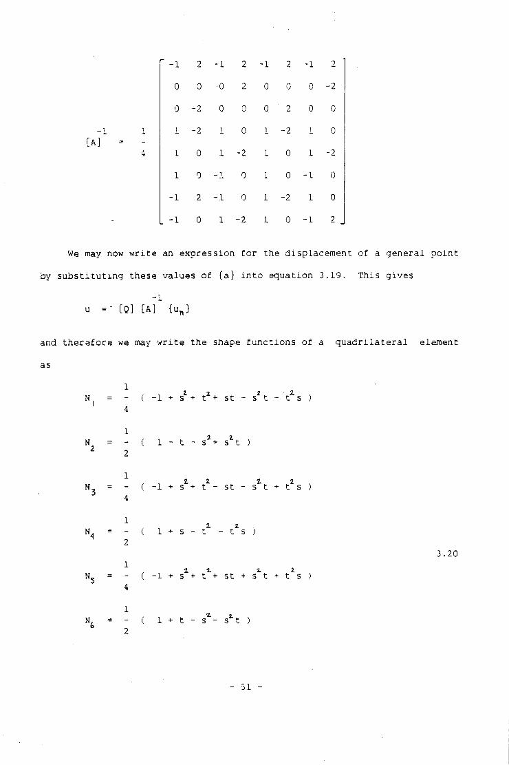
[ A ] - -
1 2 - 1 2 - 1 2 - 1 2
0 0 •0 2 0 0 0 -2
0 -2 0 0 0 2 0 0
1 -2 L 0 L -2 L 0
1 0 1 -2 1 0 1 -2
1 0 _ i 0 1 0 - 1 0
1 2 - 1 0 1 -2 1 0
1 0 1 -2 1 0 - 1 2
We may now w r i t e an e x p r e s s i o n f o r t h e d i s p l a c e m e n t o f a g e n e r a l p o i n t
by s u b s t i t u t i n g t h e s e v a l u e s o f { a } i n t o e q u a t i o n 3.19. T h i s g i v e s
- 1 u =" [Q] [ A ] { u n }
and t h e r e f o r e we may w r i t e t h e shape f u n c t i o n s o f a q u a d r i l a t e r a l element
as
1 2 2 Z - 1 + s + t + s t - s t - t s )
2 2 1 - t - S + S t )
1 Z I 2 - l + s + t - s t - s t + t s )
1 + s - t - t s )
3.20 1 % a. z
- l + s + t + s t + s t + t s )
1 + t - s2"- s x t )
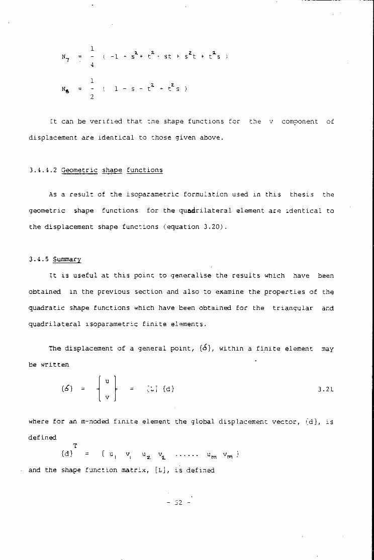
N 7 = - ( - 1 t S l+ t 1 - St t S*t + tN ) 4
1 N 6 = - ( 1 - 3 - t Z + t Z s )
2
I t can be v e r i f i e d t h a t t h e shape f u n c t i o n s f o r t h e v component o f
d i s p l a c e m e n t a r e i d e n t i c a l t o t h o s e g i v e n above.
3.4.4.2 Geometric shape f u n c t i o n s
As a r e s u l t o f t h e i s o p a r a m e t r i c f o r m u l a t i o n used i n t h i s t h e s i s t h e
g e o m e t r i c shape f u n c t i o n s f o r t h e q u a d r i l a t e r a l element a r e i d e n t i c a l t o
t h e d i s p l a c e m e n t shape f u n c t i o n s ( e q u a t i o n 3.20).
3.4.5 Summary
I t i s u s e f u l a t t h i s p o i n t t o g e n e r a l i s e t h e r e s u l t s w h i c h have been
o b t a i n e d i n t h e p r e v i o u s s e c t i o n and a l s o t o examine t h e p r o p e r t i e s o f t h e
q u a d r a t i c shape f u n c t i o n s w h i c h have been o b t a i n e d f o r t h e t r i a n g u l a r and
q u a d r i l a t e r a l i s o p a r a m e t r i c f i n i t e e l e m e n t s .
The d i s p l a c e m e n t o f a g e n e r a l p o i n t , [ & } , w i t h i n a f i n i t e element may
be w r i t t e n
[ L ] Cd} 3.21
where f o r an m-noded f i n i t e element t h e g l o b a l d i s p l a c e m e n t v e c t o r , ( d ) , i s
d e f i n e d
{ d } C u, v u z v^
and t h e shape f u n c t i o n m a t r i x , [ L ] , i s d e f i n e d
- 52 -
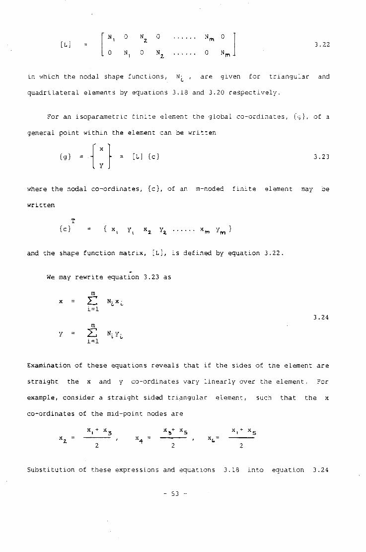
[ L ] Nx 0 0
0 N, 0 0 N r n 3 .22
i n w h i c h t h e n o d a l shape f u n c t i o n s , , a r e g i v e n f o r t r i a n g u l a r and
q u a d r i l a t e r a l elements by e q u a t i o n s 3.18 and 3.20 r e s p e c t i v e l y .
For an i s o p a r a m e t r i c f i n i t e element t h e g l o b a l c o - o r d i n a t e s , [ g } , o f a
g e n e r a l p o i n t w i t h i n t h e element can be w r i t t e n
( g ) = - [ L ] { c } 3.23
where t h e n o d a l c o - o r d i n a t e s , ( c ) , o f an m-noded f i n i t e element nnay be
w r i t t e n
T Cc} ( x . y, x z yz
and t h e shape f u n c t i o n m a t r i x , [ L ] , i s d e f i n e d by e q u a t i o n 3.22.
We may r e w r i t e e q u a t i o n 3.23 as
TL N L X L
i = l 3.24
y = m
i=l
E x a m i n a t i o n o f t h e s e e q u a t i o n s r e v e a l s t h a t i f t h e s i d e s o f t h e element a r e
s t r a i g h t t h e x and y c o - o r d i n a t e s v a r y l i n e a r l y o v e r t h e e l e m e n t . For
example, c o n s i d e r a s t r a i g h t s i d e d t r i a n g u l a r element, such t h a t t h e x
c o - o r d i n a t e s o f t h e m i d - p o i n t nodes a r e
x,+ x 3 X 3 + X S x,+ x 5
S u b s t i t u t i o n o f t h e s e e x p r e s s i o n s and e q u a t i o n s 3.18 i n t o e q u a t i o n 3.24
- 53
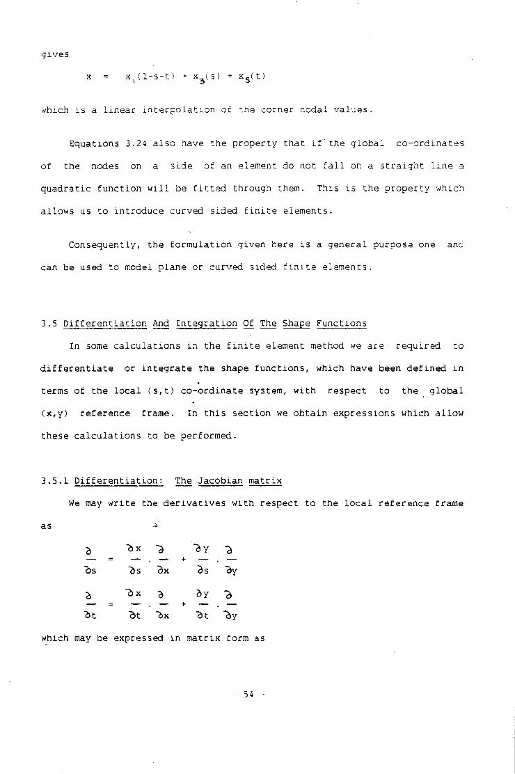
g i v e s
x = x ^ l - s - t ) + x ( s ) + x s ( t )
w hich i s a l i n e a r i n t e r p o l a t i o n o f t h e c o r n e r n o d a l v a l u e s .
E q u a t i o n s 3.24 a l s o have t h e p r o p e r t y t h a t i f t h e g l o b a l c o - o r d i n a t e s
o f t h e nodes on a s i d e o f an element do n o t f a l l on a s t r a i g h t l i n e a
q u a d r a t i c f u n c t i o n w i l l be f i t t e d t h r o u g h them. T h i s i s t h e p r o p e r t y w h i c h
a l l o w s us t o i n t r o d u c e c u r v e d s i d e d f i n i t e e l e m e n t s .
C o n s e q u e n t l y , t h e f o r m u l a t i o n g i v e n here i s a g e n e r a l p u r p o s e one anc
can be used t o model p l a n e o r c u r v e d s i d e d f i n i t e e l e m e n t s .
3.5 D i f f e r e n t i a t i o n And I n t e g r a t i o n Of The Shape F u n c t i o n s
I n some c a l c u l a t i o n s i n t h e f i n i t e element method we a r e r e q u i r e d t o
d i f f e r e n t i a t e o r i n t e g r a t e t h e shape f u n c t i o n s , w h i c h have been d e f i n e d i n
terms o f t h e l o c a l ( s , t ) c o - o r d i n a t e system, w i t h r e s p e c t t o t h e g l o b a l
( x , y ) r e f e r e n c e frame. I n t h i s s e c t i o n we o b t a i n e x p r e s s i o n s w h i c h a l l o w
t h e s e c a l c u l a t i o n s t o be p e r f o r m e d .
3.5.1 D i f f e r e n t i a t i o n : The J a c o b i a n m a t r i x
We may w r i t e t h e d e r i v a t i v e s w i t h r e s p e c t t o t h e l o c a l r e f e r e n c e frame
as
£ "bx "5 1 y
~bs "3s Bx ds "by
2, "bx 2i 2>y
b t "dt "bx "St "by
which may be expressed i n m a t r i x f o r m as
- 54 -
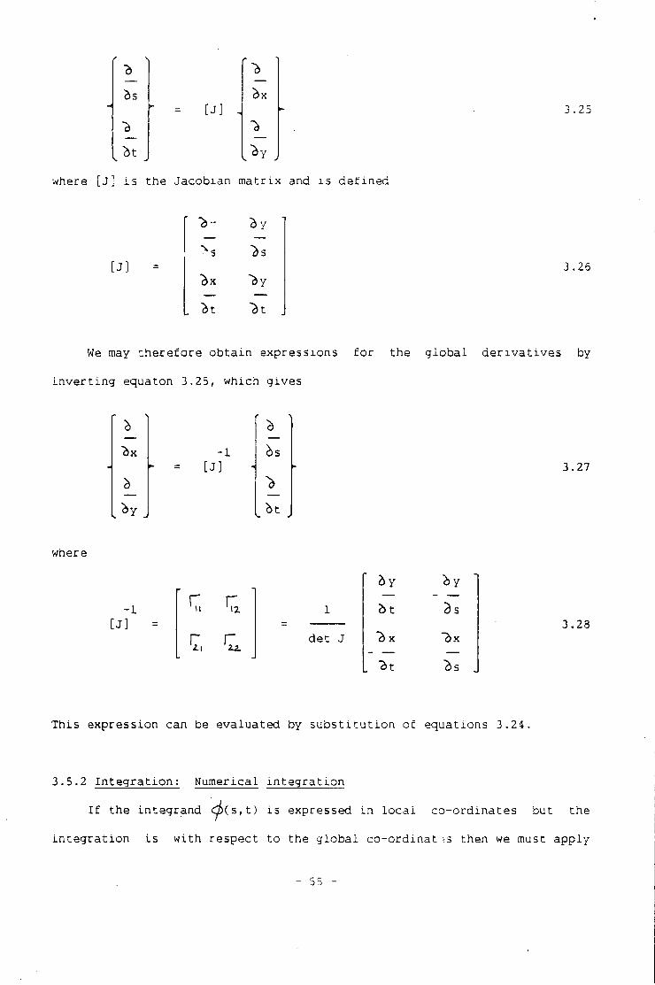
b t
[ J ] ,
I ^ y I
3 .25
where [ J ] i s t h e J a c o b i a n m a t r i x and i s d e f i n e d
[ J ] % s
^ x
3 y
^ s
^ t
3 .26
We may t h e r e f o r e o b t a i n e x p r e s s i o n s f o r t h e g l o b a l d e r i v a t i v e s by
i n v e r t i n g equaton 3.25, w h i c h g i v e s
- 1 [ J ]
bt
3.27
where
- 1 [ J ]
1 , ^ d e t J
2>y
b t
^ x
* y
3s
^ s
3.28
T h i s e x p r e s s i o n can be e v a l u a t e d by s u b s t i t u t i o n o f e q u a t i o n s 3.24.
3.5.2 I n t e g r a t i o n : N u m e r i c a l i n t e g r a t i o n
I f t h e i n t e g r a n d c ^ ( s , t ) i s exp r e s s e d i n l o c a l c o - o r d i n a t e s b u t t h e
i n t e g r a t i o n i s w i t h r e s p e c t t o t h e g l o b a l c o - o r d i n a t ?s then we must a p p l y
- 55 -
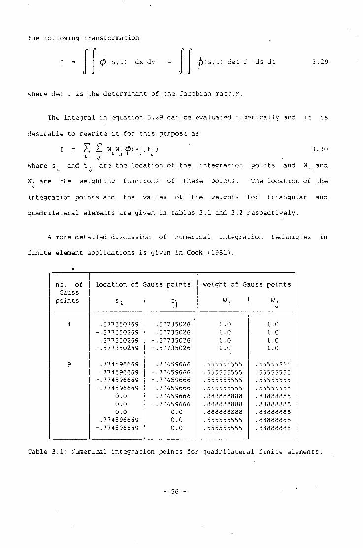
t h e f o l l o w i n g t r a n s f o r m a t i o n
I = (p ( s, t ) dx dy t ) d e t J ds d t 3 .29
where d e t J i s t h e d e t e r m i n a n t o f t h e J a c o b i a n m a t r i x .
The i n t e g r a l i n e q u a t i o n 3.29 can be e v a l u a t e d n u m e r i c a l l y and i t i s
d e s i r a b l e t o r e w r i t e i t f o r t h i s p urpose as
I = X Z! W. W. 4>(s- , t ; ) 3.30 •L t j T c J where s. and t - a r e t h e l o c a t i o n o f t h e i n t e g r a t i o n p o i n t s and W- and c 0 <-Wj a r e t h e w e i g h t i n g f u n c t i o n s o f t h e s e p o i n t s . The l o c a t i o n o f t h e
i n t e g r a t i o n p o i n t s and t h e v a l u e s o f t h e w e i g h t s f o r t r i a n g u l a r and
q u a d r i l a t e r a l elements a r e g i v e n i n t a b l e s 3.1 and 3.2 r e s p e c t i v e l y .
A more d e t a i l e d d i s c u s s i o n o f n u m e r i c a l i n t e g r a t i o n t e c h n i q u e s i n
f i n i t e , element a p p l i c a t i o n s i s g i v e n i n Cook ( 1 9 8 1 ) .
no. o f l o c a t i o n o f Gauss p o i n t s w e i g h t o f Gauss p o i n t s Gauss
p o i n t s 'j
W-W j
4 .577350269 .57735026 ' 1.0 1.0 -.577350269 .57735026 1.0 1.0 .577350269 -.57735026 1.0 1.0
-.577350269 -.57735026 1.0 1.0
9 .774596669 .77459666 .555555555 .55555555 .774596669 -.77459666 .555555555 .55555555
-.774596669 -.77459666 . 5555555 55 .55555555 -.774596669 .77459666 .55 5555555 .55555555
0.0 .77459666 .383888888 .88888888 0.0 -.77459666 .888888888 .88388888 0.0 0.0 .388888888 .88838888
.774596669 0.0 .555555555 .88888388 -.774596669 0.0 .555555555 .88888838
T a b l e 3.1: N u m e r i c a l i n t e g r a t i o n p o i n t s f o r q u a d r i l a t e r a l f i n i t e e l e m e n t s .
- 56 -
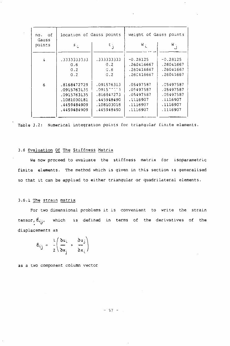
no. o f l o c a t i o n o f Gauss p o i n t s w e i g h t o f Gauss p o i n t s Gauss
p o i n t s 3 • W • W • J
4 .3333333333 .333333333 -0.28125 -0 .28125 0.6 0.2 .260416667 .26041667 0.2 0.6 .260416667 .26041667 0.2 0.2 .260416667 .26041667
6 .8168472729 .091576313 .05497587 .05497587 .0915763135 .0915""." 3 .05497587 .05497587 .0915763135 .816347273 .05497587 .05497587 .1081030181 . 445948490 .1116907 . 1116907 .4459484909 .108103018 .1116907 .1116907 .4459484909 . 445948490 .1116907 .1116907
T a b l e 3.2: N u m e r i c a l i n t e g r a t i o n p o i n t s f o r t r i a n g u l a r f i n i t e e l e m e n t s .
3.6 E v a l u a t i o n Of The S t i f f n e s s M a t r i x
We now p r o c e e d t o e v a l u a t e t h e s t i f f n e s s m a t r i x f o r i s o p a r a m e t r i c
f i n i t e e l e m e n t s . The method w h i c h i s g i v e n i n t h i s s e c t i o n i s g e n e r a l i s e d
so t h a t i t can be a p p l i e d t o e i t h e r t r i a n g u l a r o r q u a d r i l a t e r a l e l e m e n t s .
3.6.1 The s t r a i n m a t r i x
For two d i m e n s i o n a l problems i t i s c o n v e n i e n t t o w r i t e t h e s t r a i n
t e n s o r , w h i c h i s d e f i n e d i n terms o f t h e d e r i v a t i v e s o f t h e
d i s p l a c e m e n t s as
£. - + ^ ^ 2\"2>Xj + b x c
as a two component column v e c t o r
- 57 -
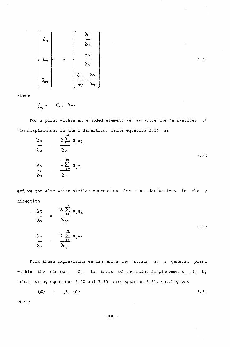
- £
where
b x
b v
cbu ~bv
b y ~bx
3.31
For a p o i n t w i t h i n an m-noded element we may w r i t e t h e d e r i v a t i v e s o f
t h e d i s p l a c e m e n t i n t h e x d i r e c t i o n , u s i n g e q u a t i o n 3.24, as
^ u
*x ^ x
m b v
hx
3.32
and we can a l s o w r i t e s i m i l a r e x p r e s s i o n s f o r t h e d e r i v a t i v e s i n t h e y
d i r e c t i o n
In
^ v
3.33
^ H N L=.l
From t h e s e e x p r e s s i o n s we can w r i t e t h e s t r a i n a t a g e n e r a l p o i n t
w i t h i n t h e element, {£}, i n terms o f t h e n o d a l d i s p l a c e m e n t s , { d } , by
s u b s t i t u t i n g e q u a t i o n s 3.32 and 3.33 i n t o e q u a t i o n 3.31, which g i v e s
{£} = [ B ] Cd} 3.34
where
- 58 -
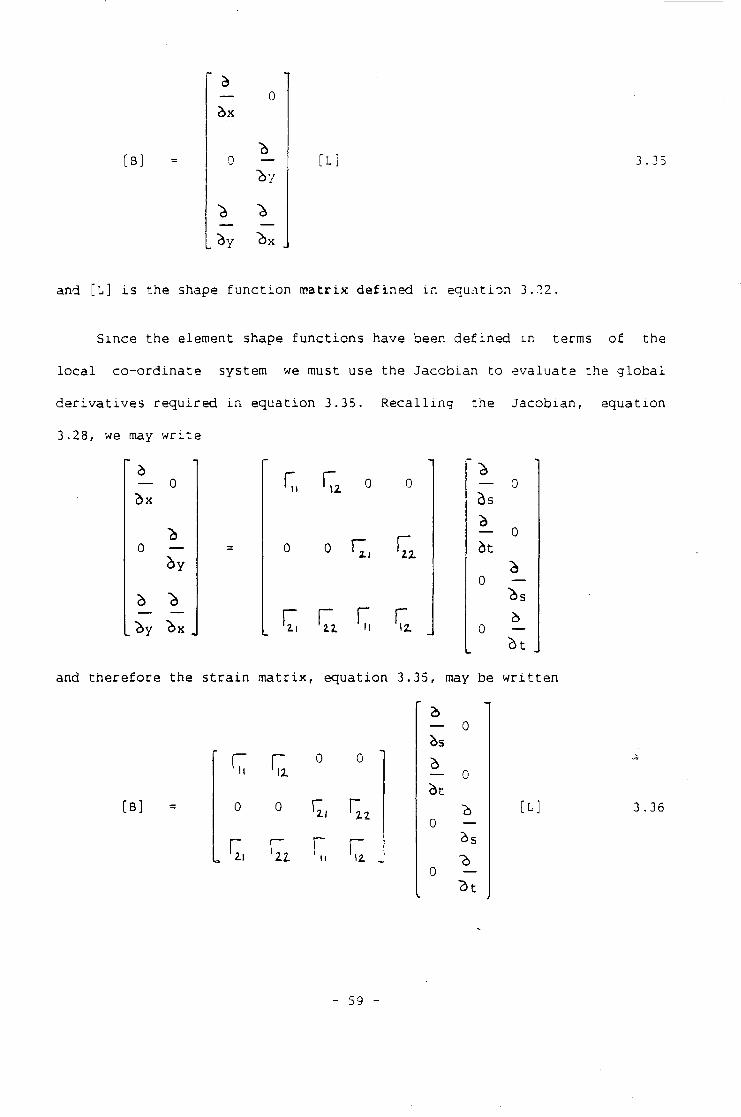
[ B ]
b — 0 bx
"b
0 —
b y
[ L ] 3.3:
and [l] i s t h e shape f u n c t i o n m a t r i x d e f i n e d i n e q u a t i o n 3.22,
S i n c e t h e element shape f u n c t i o n s have been d e f i n e d i n terms o f t h e
l o c a l c o - o r d i n a t e system we must use t h e J a c o b i a n t o e v a l u a t e t h e g l o b a l
d e r i v a t i v e s r e q u i r e d i n e q u a t i o n 3.35. R e c a l l i n g t h e J a c o b i a n , e q u a t i o n
3.28, we may w r i t e
" b — 0 b x
"b 0 — =
b "b
_ y ^ x .
0
r r r r
— o bs b — 0 b t
b o —
^>s h
0 — b t
and t h e r e f o r e t h e s t r a i n m a t r i x , e q u a t i o n 3.35, may be w r i t t e n
[ B ]
r r 0 0
0 0 ^ riz
r r r r
b — o bs b — 0 b t
"b 0 —
bs
2>t
[ L ; 3.3c
- 59 -

T h i s e x p r e s s i o n can be e v a l u a t e d i f t h e a p p r o p r i a t e shape f u n c t i o n s ,
e q u a t i o n 3.22, a r e s u b s t i t u t e d i n t o i t .
3.6.2 The e l a s t i c i t y m a t r i x
For two d i m e n s i o n a l problems i t i s c o n v e n i e n t t o w r i t e t h e s t r e s s
t e n s o r , w h i c h i s d e f i n e d i n terms o f t h e s t r a i n t h r o u g h Hooka's law as
X e + 2 u £..
where A and u a r e Lame's c o n s t a n t s and &.. i s t h e Kroneker d e l t a f u n c t i o n ,
as a two component column v e c t o r
C<r} Ox
3.37
The s t r a i n s may be w r i t t e n i n terms o f t h e s t r e s s e s , i n c l u d i n g any
i n i t i a l s t r a i n s , £ Q , i n terms o f Poisson's r a t i o , x> , and Young's modulus,
E, as
1
E
2 (l+\»
For t h e two d i m e n s i o n a l case o f p l a n e s t r a i n t h e s t r e s s i n t h e z
d i r e c t i o n i s
9 ( cr + cr )
which upon s u b s t i t u t i o n i n t o e q u a t i o n 3.37 g i v e s
- 60 -
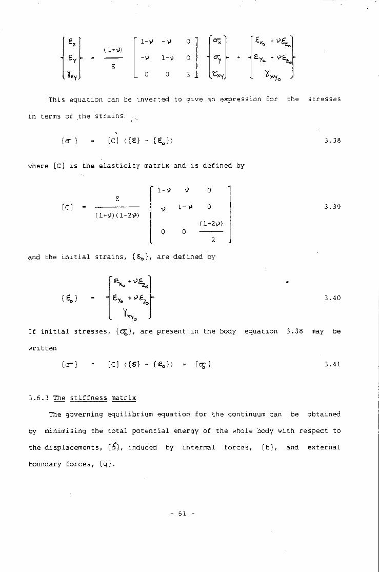
u
( l + v>) 1-V -v> 0
-v> 1-V 0 > cr 7 +
0 0 2
T h i s e q u a t i o n can be i n v e r t e d t o g i v e an e x p r e s s i o n f o r t h e s t r e s s e s
i n terms o f t h e s t r a i n s .
{o- } = [C] ((£} - ( £ J )
where [C] i s t h e e l a s t i c i t y m a t r i x and i s d e f i n e d by
[C] = ( i + * ) ( i - 2 * )
l - v \>
1- V
0
0
(l-2v»
and t h e i n i t i a l s t r a i n s , (£*>}, a r e d e f i n e d by
3 .38
3.39
- £y a +v>£, f- 3.40
I f i n i t i a l s t r e s s e s , [0~], a r e p r e s e n t i n t h e body e q u a t i o n 3.38 may be
w r i t t e n
Co-} = [C] ((£} - ( % } ) + { C T } 3.41
3.6.3 The s t i f f n e s s m a t r i x
The g o v e r n i n g e q u i l i b r i u m e q u a t i o n f o r t h e c o n t i n u u m can be o b t a i n e d
by m i n i m i s i n g t h e t o t a l p o t e n t i a l e n e r g y o f t h e whole body w i t h r e s p e c t t o
t h e d i s p l a c e m e n t s , [£}, i n d u c e d by i n t e r n a l f o r c e s , ( b } , and e x t e r n a l
boundary f o r c e s , Cq}.
- 61 -
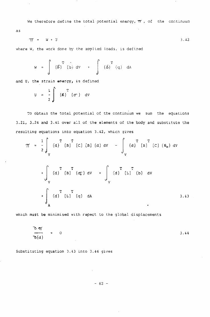
We t h e r e f o r e d e f i n e t h e t o t a l p o t e n t i a l energy, TT , o f t h e c o n t i n u u m
as
TT = W + U
where W, t h e work done by t h e a p p l i e d l o a d s , i s d e f i n e d
3.42
{8} [ b ] dV +
and U, t h e s t r a i n e n e r g y , i s d e f i n e d
{6} { q } dA
U = (£} (O- } dV
To o b t a i n t h e t o t a l p o t e n t i a l o f t h e c o n t i n u u m we sum t h e e q u a t i o n s
3.21, 3.24 and 3.41 o v e r a l l o f t h e elements o f t h e body and s u b s t i t u t e t h e
r e s u l t i n g e q u a t i o n s i n t o e q u a t i o n 3.42, w h i c h g i v e s
T T Cd} [ B ] [C] [ B ] (d} dV
T T Cd} [ B ] [C] [ 6 0 ] dV
T T [ d } [ B ] {07} dV +
T T { d } [ L ] { b } dV
T T (d} [ L ] { q } dA 3.43
w h i c h must be m i n i m i s e d w i t h r e p e c t t o t h e g l o b a l d i s p l a c e m e n t s
"b T f
-o{d} 3 .44
S u b s t i t u t i n g e q u a t i o n 3.43 i n t o 3.44 g i v e s
- 62 -
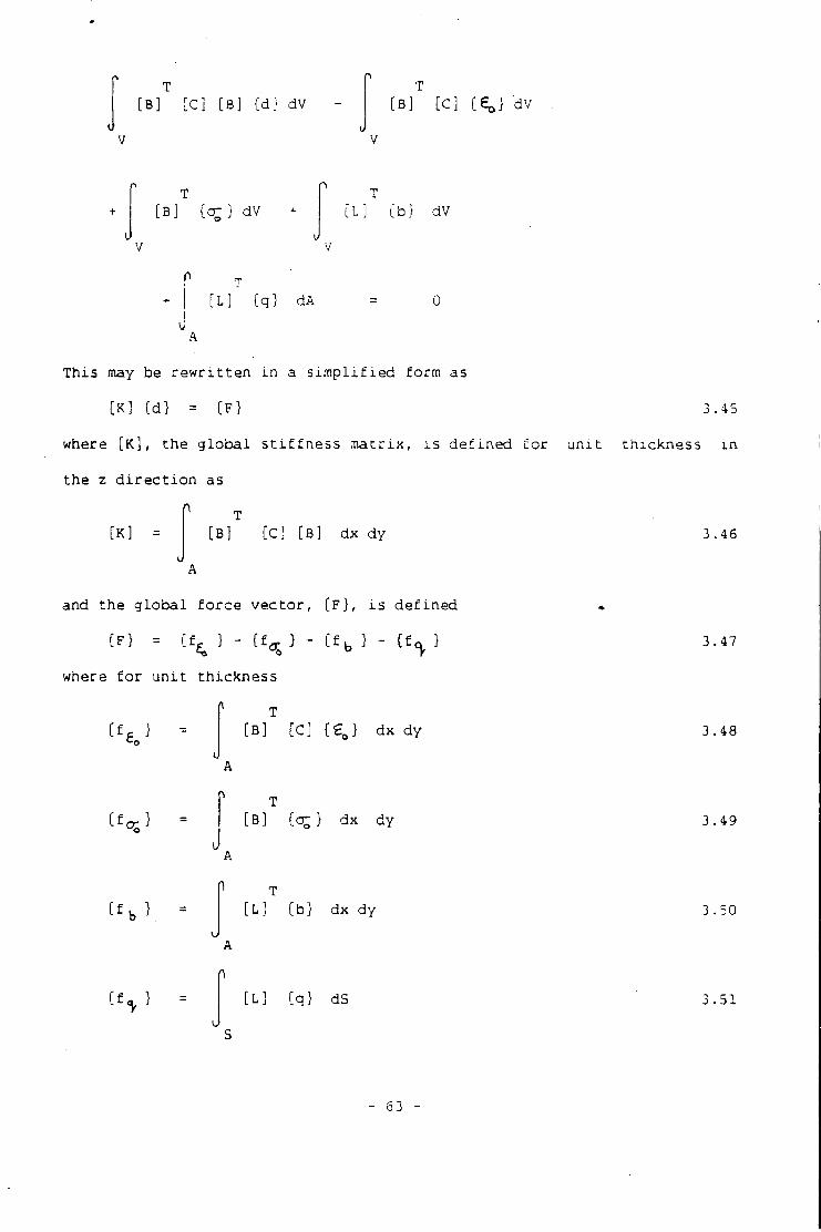
[ B ] [ C ] [ B ] ( d ) dV :B] [ C ] [ e j dv
[B] ( c r ) dV + [ L ] ( b ) dV
? T + | [ L ] { q } dA = 0
I
A
T h i s may be r e w r i t t e n i n a s i m p l i f i e d f o r m as
[ K ] { d } = ( F ) 3.45
where [ K ] , t h e g l o b a l s t i f f n e s s m a t r i x , i s d e f i n e d f o r u n i t t h i c k n e s s i n
t h e z d i r e c t i o n as
[K] [ B ] [C] [ B ] dx dy 3.46
and t h e g l o b a l f o r c e v e c t o r , ( F } , i s d e f i n e d
( F ) = ( f ^ } " [ f a r ) " Cf b } - { f < )
where f o r u n i t t h i c k n e s s
3.47
[B] [C] ( £ J dx dy 3.48
[B] ( o r } dx dy 3.49
[ L ] ( b ) dx dy 3.50
tty) [ L ] { q } dS 3.51
- 63 -
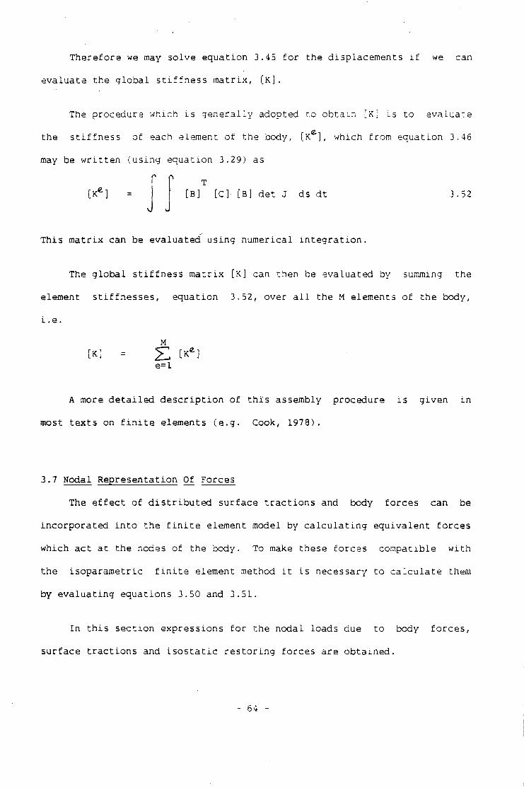
T h e r e f o r e we may s o l v e e q u a t i o n 3.45 f o r t h e d i s p l a c e m e n t s i f we can
e v a l u a t e t h e g l o b a l s t i f f n e s s m a t r i x , [ K ] .
The p r o c e d u r e w h i c h i s g e n e r a l l y a d o p t e d t o o b t a i n [ K ] i s t o e v a l u a t e
t h e s t i f f n e s s o f each element o f t h e body, [ K a ] , w h i c h f r o m e q u a t i o n 3.46
may be w r i t t e n ( u s i n g e q u a t i o n 3.29) as
[ K E ] = T
[B] [C] [ B ] d e t J ds d t 3.52
T h i s m a t r i x can be e v a l u a t e d u s i n g n u m e r i c a l i n t e g r a t i o n .
The g l o b a l s t i f f n e s s m a t r i x [K] can t h e n be e v a l u a t e d by summing t h e
element s t i f f n e s s e s , e q u a t i o n 3.52, o v e r a l l t h e M elements o f t h e body,
i . e .
M [K] = 2
e = l
A more d e t a i l e d d e s c r i p t i o n o f t h i s assembly p r o c e d u r e i s g i v e n i n
most t e x t s on f i n i t e e l ements ( e . g . Cook, 19 7 8 ) .
3.7 Nodal R e p r e s e n t a t i o n Of Forces
The e f f e c t o f d i s t r i b u t e d s u r f a c e t r a c t i o n s and body f o r c e s can be
i n c o r p o r a t e d i n t o t h e f i n i t e element model by c a l c u l a t i n g e q u i v a l e n t f o r c e s
w h i c h a c t a t t h e nodes o f t h e body. To make t h e s e f o r c e s c o m p a t i b l e w i t h
t h e i s o p a r a m e t r i c f i n i t e element method i t i s n e c e s s a r y t o c a l c u l a t e them
by e v a l u a t i n g e q u a t i o n s 3.50 and 3.51.
I n t h i s s e c t i o n e x p r e s s i o n s f o r t h e n o d a l l o a d s due t o body f o r c e s ,
s u r f a c e t r a c t i o n s and i s o s t a t i c r e s t o r i n g f o r c e s a r e o b t a i n e d .
- 64 -
3.7.1 Body f o r c e s
The body f o r c e v e c t o r , [ b ] , due t o g r a v i t y , g, ( d i r e c t e d down t h e
n e g a t i v e y a x i s ) a c t i n g upon a m a t e r i a l o f d e n s i t y f> i s g i v e n by
0 [ b }
T h e r e f o r e i f we e v a l u a t e t h i g l o b a l body f o r c e v e c t o r , ( f ^ l , g i v e n r y
e q u a t i o n 3.50, a t each element o f t h e body we may o b t a i n t h e element, boc<"
f o r c e v e c t o r , ( f e } , w h i c h i s d e f i n e d
T f ~\ 0
[ L ] - *> - d e t J ds d t 3.53
which must be e v a l u a t e d by n u m e r i c a l i n t e g r a t i o n .
The g l o b a l body f o r c e v e c t o r ( f ^ } can be e v a l u a t e d by summing e q u a t i o n
3.53 o v e r a l l t h e ele m e n t s o f t h e body.
3.7.2 S u r f a c e t r a c t i o n
I n t h i s s e c t i o n e x p r e s s i o n s f o r t h e n o d a l r e p r e s e n t a t i o n o f f o r c e s due
t o s u r f a c e l o a d s a r e o b t a i n e d . These f o r c e s , by d e f i n i t i o n , a c t o n l y upon
an edge o f an element and i t i s c o n v e n i e n t i f we p e r f o r m t h e r e q u i r e d
c a l c u l a t i o n s i n a s p e c i a l l o c a l c o - o r d i n a t e system.
3.7.2.1 The l o c a l c o - o r d i n a t e system
C o n s i d e r t h e edge o f an element formed by nodes 1, 2 and 3 w h i c h have
t h e n o d a l c o - o r d i n a t e s ( x , ,y ( ) , ( x ^ / Y j a n c ^ <- X3'^5' ) r e s P e c t ^ v e l Y • Then we
may l e t t h i s edge d e f i n e t h e l o c a l c o - o r d i n a t e s - a x i s which has i t s o r i g i n
a t node 2 and i t s p o s i t i v e a x i s d i r e c t e d t o w a r d s node 1 ( f i g u r e 3 . 5 ) .
- 65 -
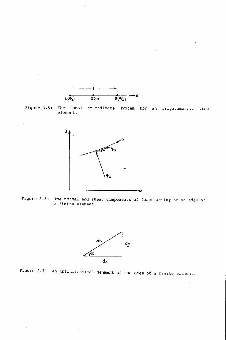
I
F i g u r e 3.5: The l o c a l c o - o r d i n a t e system Cor an i s o p a r a m e t r i c L i n e e l e m e n t .
F i g u r e 3.6: The normal and shear components o f f o r c e a c t i n g ac an edge o f a f i n i t e e l e m e n t .
F i g u r e 3.7: An i n f i m t e s s i m a l segment o f t h e edge o f a f i n i t e element.
I t i s p o s s i b l e t o d e f i n e t h e q u a d r a t i c shape f u n c t i o n s o f t h i s system
as 2s — + 1 I
4 s' 3.54
s / 2s
i \ ~ t + 1 /
where £ i s t h e l e n g t h o f t h e s i d e .
We may use t h e s e shape f u n c t i o n s t o exp r e s s t h e c a r t e s i a n c o - o r d i n a t e s
( x , y ) o f a g e n e r a l p o i n t on t h e edge i n terms o f i t s n o d a l v a l u e s as
= [ L ] Cc}
where t h e shape f u n c t i o n m a t r i x i s
3.55
[ L ] = N, 0 N 2 0 N 3 0
0 N( 0 N 2 0 N
and { c } , t h e n o d a l c o - o r d i n a t e v e c t o r , i s
T ( c ) ( x, y ( x z y z x 3 y 3 }
I t i s a l s o n e c e s s a r y t o use a d i f f e r e n t n u m e r i c a l i n t e g r a t i o n scheme
when u s i n g t h i s l o c a l c o - o r d i n a t e system such t h a t
<£(s) ds = £ W. (^>(sc 3.56
where t h e l o c a t i o n o f t h e i n t e g r a t i o n p o i n t s and t h e i r w e i g h t s a r e g i v e n i n
t a b l e 3.3.
- 66 -
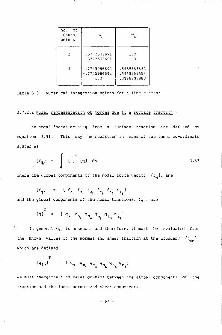
no. o f Gauss
p o i n t s s.
2 .5773502691 1.0 -.5773502691 1.0
3 .7745966692 .5555555555 -.7745966692 .5555o555 5 5
.3338838888
T a b l e 3.3: N u m e r i c a l i n t e g r a t i o n p o i n t s f o r a l i n e e l e m e n t .
3.7.2.2 Nodal r e p r e s e n t a t i o n o f f o r c e s due t o a s u r f a c e t r a c t i o n -
The n o d a l f o r c e s a r i s i n g f r o m a s u r f a c e t r a c t i o n a r e d e f i n e d by
e q u a t i o n 3.51. T h i s may be r e w r i t t e n i n terms o f t h e l o c a l c o - o r d i n a t e
system as
T [ L ] { q } ds 3.57
where t h e g l o b a l components o f t h e n o d a l f o r c e v e c t o r , ( f , ^ } , a r e
T
and t h e g l o b a l components o f t h e n o d a l t r a c t i o n s , ( q ) , a r e
T Cq) = C q x q y q% q y q x q y }
I n g e n e r a l {q} i s unknown, and t h e r e f o r e , i t must be e v a l u a t e d from
t h e known v a l u e s o f t h e n o r m a l and shear t r a c t i o n a t t h e boundary, Cq 5 n}/
which a r e d e f i n e d
T Cq s n} - C q q q q q s q }
1 > i e. 3 s
We must t h e r e f o r e f i n d r e l a t i o n s h i p s between t h e g l o b a l components o f t h e
t r a c t i o n and t h e l o c a l n o r m a l and shear components.
- 67 -
U s i n g f i g u r e 3.7 we may w r i t e t h e r e l a t i o n s h i p between t h e s e a t a
g e n e r a l p o i n t as
q, 3.53
COScC - s i n c e
) s inoC cosoC .
From f i g u r e 3.8, however, we know t h a t
dx = cos pC ds
dy = s i n oC ds
and t h e r e f o r e we may r a w i t e e q u a t i o n 3.58 as
qv i n w h i c h
[R ' ] -
dx dy
ds ds
dy dx
ds ds
3.59
E v a l u a t i n g e q u a t i o n 3.59 a t t h e t h r e e nodes on t h e boundary we o b t a i n
Cq} = [R] ( q 5 n ) 3.60
i n w h i c h
[R'J 0 0
[R] = 0 [R'J 0
0 0 [R' ]
We t h e r e f o r e o b t a i n t h e d e s i r e d f o r c e e q u a t i o n by s u b s t i t u t i n g e q u a t i o n
3.60 i n t o e q u a t i o n 3.57, g i v i n g
T [ L ] [R] ( q } ds 3 .61
whic h must be e v a l u a t e d by n u m e r i c a l i n t e g r a t i o n .
- 68 -
3.7.2.3 I s o s t a t i c c o m p e n s a t i o n
The s i t u a t i o n where t h e body i s bounded by a f l u i d i s now c o n s i d e r e d .
I n t h i s case t h e d i s p l a c e m e n t s o f t h e body a r e r e s i s t e d by h y d r o s t a t i c
r e s t o r i n g f o r c e s (Dean, 1973).
The p r e s s u r e i n a f l u i d , q, r e s i s t i n g a v e r t i c a l d i s p l a c e m e n t , v, i s
q = - fi Sf v
where p i s t h e d e n s i t y o f t h e f l u i d and g i s t h e a c c e l e r a t i o n due t o
g r a v i t y . T h i s r e s t o r i n g f o r c e a c t s normal t o t h e boundary o f t h e element,
and t h e r e f o r e , we may w r i t e t h e no r m a l and shear f o r c e v e c t o r , C q S r ) } f as
( q ^ } = pq { d } 3.62
where
T Cd} = C 0 v ( 0 v z 0 v 3 }
We t h e r e f o r e o b t a i n the d e s i r e d e x p r e s s i o n by s u b s t i t u t i n g equation
3.62 i n t o equation 3.61, g i v i n g
Cf^} = [ K z ] Cd} 3.63
where
[ K T ] [ L ] [R] ds
which may be i n c o r p o r a t e d as a f o r c e i n the g l o b a l s t i f f n e s s equation
(equation 3.45)
[ K ] Cd}
so t h a t by s u b s t i t u t i o n of equation 3.61 we o b t a i n
[ K ] Cd}
and t h e r e f o r e
f F } = [K - K r ] Cd}
- 69 -
C F + • [ K x ] ( d } )
We can c o n s e q u e n t l y i n c o r p o r a t e i s o s t a t i c r e s t o r i n g f o r c e s i n t h e
model by s u b t r a c t i n g t h e i s o s t a t i c m a t r i x f r o m t h e g l o b a l s t i f f n e s s m a t r i x ,
[ K ] .
3.8 Thermal S t r e s s e s
The - a f f e c t of. t h e r m a l volume changes can be i n c o r p o r a t e d i n t o t h e
f i n i t e element model u s i n g t h e i n i t i a l s t r a i n approach (Ccck, 1981). For
p l a n e s t r a i n we can t h e r e f o r e w r i t e t h e i n i t i a l s t r a i n , {€,,}, as
(So) ( l + v>) - ^ A T -
where d. i s t h e volume c o e f f i c i e n t o f t h e r m a l e x p a n s i o n and A T i s t h e
t e m p e r a t u r e change.
These i n i t i a l s t r a i n s can be i n c o r p o r a t e d i n t o t h e f i n i t e element
c a l c u l a t i o n s by e v a l u a t i n g t h e i n i t i a l s t r a i n f o r c e v e c t o r ( e q u a t i o n 3 . 4 8 ) .
S o l u t i o n o f t h e s t i f f n e s s e q u a t i o n t h e n y i e l d s t h e s t r a i n i n t h e body, so
t h a t t h e t h e r m a l s t r e s s can be c a l c u l a t e d f r o m
Co-} = [c] ((£} - ce Q}) where, f o r p l a n e s t r a i n ,
= v>(cy+cr.) " E*AT
3 .9 V i s c o - e l a s t i c A n a l y s i s
V i s c o - e l a s t i c b e h a v i o u r can be i n c o r p o r a t e d i n t o t h e f i n i t e element
method by u s i n g t h e i n i t i a l s t r a i n a p r o a c h ( Z i e n k i e w i c z e t a l , 1 9 6 8 ) .
- 70 -
The s t r a i n r a t e t e n s o r , ( }, a t a g e n e r a l p o i n t i n a Maxwell body
w i t h v i s c o s i t y , C| , i s
( W ) 07-
2 1 3.64
where OT i s t h e d e v i t o r i c s t r e s s t e n s o r w h i c h i s d e f i n e d
cr'. = cr. -
The second t e r m on t h e r i g h t hand s i d e o f e q u a t i o n 3.54 i s t h e v i s c o u s
c r e e p r a t e ( £ ) c w h i c h i s d e f i n e d a t a g e n e r a l p o i n t i n t h e body as
( e Y } c
C J
1
5 - ° w
a: - c r .
where cT , t h e h y d r o s t a t i c s t r e s s , i s d e f i n e d n
(cr > c r Y + c r )
Because o f t h e e x i s t e n c e o f t h e d e v i a t o r i c s t r e s s t h e z component o f
c r e e p C^zl i s n o t z e r o . C o n s e q u e n t l y t o f u l f i l l t h e c o n d i t i o n o f p l a n e
s t r a i n i t i s n e c e s s a r y t h a t t h e t o t a l s t r a i n i n t h e z d i r e c t i o n e q u a l s
z e r o , t h a t i s
(<S - <Th ) ( l + v>)
I t i s now p o s s i b l e t o e v a l u a t e t h e t o t a l c r e e p s t r a i n (£) c.over a
t i m e s t e p t by t h e s i m p l e i n t e g r a t i o n
(£} c - ( £ ) c t
whi c h may be w r i t t e n as an i n i t i a l s t r a i n
CS 0] = ( € } c
and i n c o r p o r a t e d as a f o r c e due t o t h e i n i t i a l s t r a i n s
- 71 -
T [B ] [C] { £ ) dx dy
T h i s must be e v a l u a t e d by n u m e r i c a l i n t e g r a t i o n and added t o t h e
g l o b a l f o r c e v e c t o r . The s t i f f n e s s e q u a t i o n can t h e n be r e s o l v e d u s i n g
t h i s new f o r c e v e c t o r , w h i c h g i v e s t h e s t r e s s a t t h e end o f t h e t i m e
i n c r e m e n t , and t h e r e f o r e a new e s t i m a t e of. t h e c r e e p s t r a i n s and t h e
i n i t i a l S t r a i n f o r c e v e c t o r . The f t i . f f n e s s e q u a t i o n i s t h e n r e s o l v e d u s i n g
t h i s new f o r c e v e c t o r and t h e p r o c e d u r e i s r e p e a t e d u n t i l t h e c r e e p s t r e s s
a t t h e end o f t h e t i m e i n c r e m e n t f a l l s t o an a c c e p t a b l e l e v e l .
A more c o m p l e t e d i s c u s s i o n o f t h i s a l g o r i t h m i s g i v e n i n Park ( 1 9 8 1 ) .
- 72 -
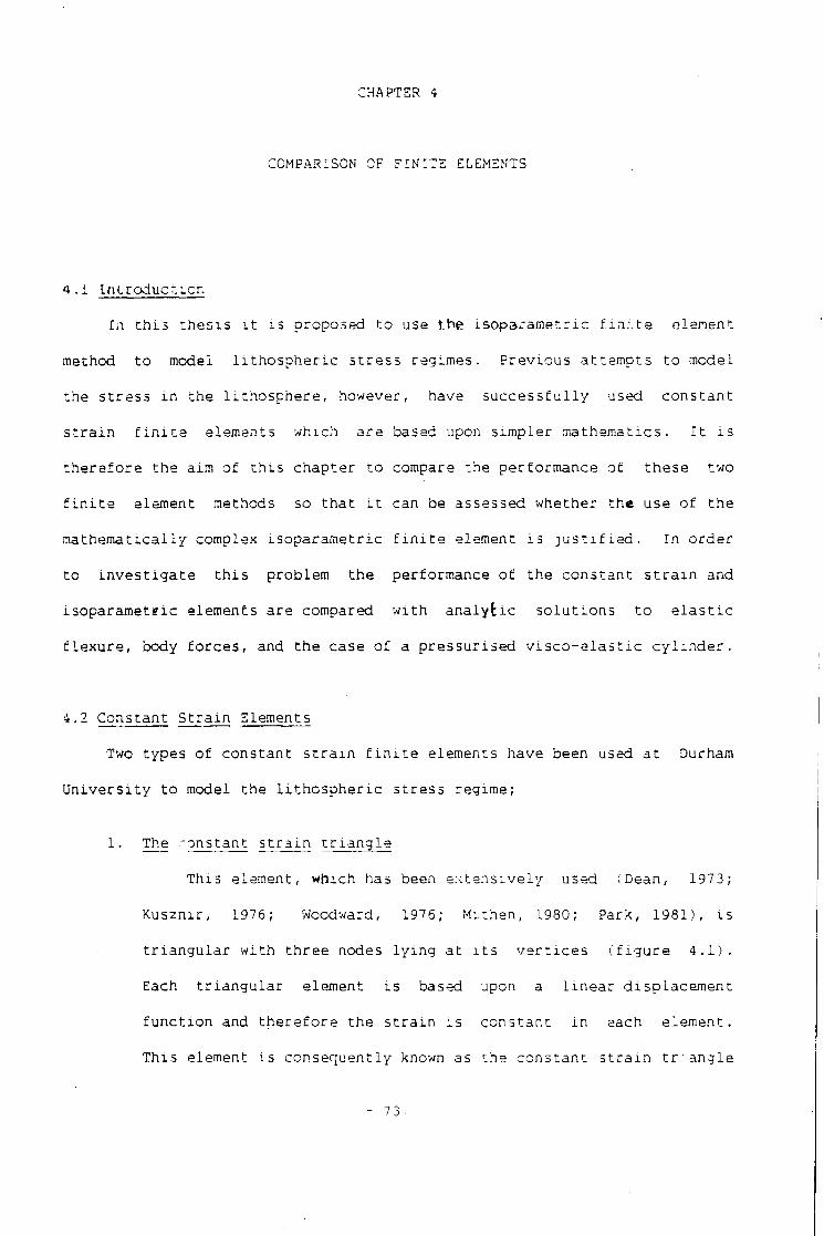
CHAPTER 4
COMPARISON OF FINITE ELEMENTS
4. i i n t r o d u c t i o n
I n t h i s t h e s i s i t i s proposed t o use t h e i s o p a r a m e t r i c f i n i t e element
method t o model l i t h o s p h e r i c s t r e s s r e g i m e s . P r e v i o u s a t t e m p t s t o model
th e s t r e s s i n t h e l i t h o s p h e r e , however, have s u c c e s s f u l l y used c o n s t a n t
s t r a i n f i n i t e elements which a r e based upon s i m p l e r m a t h e m a t i c s . I t i s
t h e r e f o r e t h e aim o f t h i s c h a p t e r t o compare t h e p e r f o r m a n c e of t h e s e two
f i n i t e element methods so t h a t i t can be assessed whether t h e use o f t h e
m a t h e m a t i c a l l y complex i s o p a r a m e t r i c f i n i t e element i s j u s t i f i e d . I n o r d e r
t o i n v e s t i g a t e t h i s p r o b l e m t h e performance o f t h e c o n s t a n t s t r a i n and
i s o p a r a m e t r i c elements a r e compared w i t h a n a l y t i c s o l u t i o n s t o e l a s t i c
f l e x u r e , body f o r c e s , and t h e case o f a p r e s s u r i s e d v i s c o - e l a s t i c c y l i n d e r .
4.2 C o n s t a n t S t r a i n Elements
Two t y p e s o f c o n s t a n t s t r a i n f i n i t e elements have been used a t Durham
U n i v e r s i t y t o model t h e l i t h c s p h e r i c s t r e s s r egime;
1. The - o n s t a n t s t r a i n t r i a n g l e
T h i s element, which has been e x t e n s i v e l y used (Dean, 1973;
K u s z n i r , 1976; Woodward, 1976; M i t h e n , 1980; Park, 1 9 8 1 ) , i s
t r i a n g u l a r w i t h t h r e e nodes l y i n g a t i t s v e r t i c e s ( f i g u r e 4 . 1 ) .
Each t r i a n g u l a r element i s based upon a l i n e a r d i s p l a c e m e n t
f u n c t i o n and t h e r e f o r e t h e s t r a i n i s c o n s t a n t i n each e l e m e n t .
T h i s element i s c o n s e q u e n t l y known as t h e c o n s t a n t s t r a i n t r .angle
- 73 • -
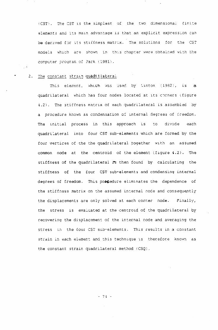
(CST). The CST i s t h e s i m p l e s t o f t h e two d i m e n s i o n a l f i n i t e
elements and i t s main advantage i s t h a t an e x p l i c i t e x p r e s s i o n can
be d e r i v e d f ^ r i t s s t i f f n e s s m a t r i x . The s o l u t i o n s f o r t h e CST
models w h i c h a r e shown i n t h i s c h a p t e r were o b t a i n e d w i t h t h e
computer program o f Park ( 1 9 8 1 ) .
2. The c o n s t a n t s t r a i n q u a d r i l a t e r a l
T h i s element, whLch was used by L i n t o n ( 1 9 3 2 ) , i s a
q u a d r i l a t e r a l w h i c h has f o u r nodes l o c a t e d a t i t s c o r n e r s ( f i g u r e
4.2). The s t i f f n e s s m a t r i x o f each q u a d r i l a t e r a l i s assembled by
a p r o c e d u r e known as c o n d e n s a t i o n o f i n t e r n a l d e g rees o f freedom.
The i n i t i a l p r o c e s s i n t h i s approach i s t o d i v i d e each
q u a d r i l a t e r a l i n t o f o u r CST sub-elements which a r e formed by t h e
f o u r v e r t i c e s o f t h e t h e q u a d r i l a t e r a l t o g e t h e r w i t h an assumed
common node a t t h e c e n t r o i d o f t h e element ( f i g u r e 4 . 2 ) . The
s t i f f n e s s o f t h e q u a d r i l a t e r a l r>s t h e n f o u n d by c a l c u l a t i n g t h e
s t i f f n e s s o f t h e f o u r CST sub-elements and c o n d e n s i n g i n t e r n a l
degrees o f freedom. T h i s p r o c e d u r e e l i m i n a t e s t h e dependence o f
t h e s t i f f n e s s m a t r i x on t h e assumed i n t e r n a l node and c o n s e q u e n t l y
t h e d i s p l a c e m e n t s a r e o n l y s o l v e d a t each c o r n e r node. F i n a l l y ,
t h e s t r e s s i s e v a l u a t e d a t t h e c e n t r o i d o f t h e q u a d r i l a t e r a l by
r e c o v e r i n g t h e d i s p l a c e m e n t o f t h e i n t e r n a l node and a v e r a g i n g t h e
s t r e s s i n t h e f o u r CST sub-elements. T h i s r e s u l t s i n a c o n s t a n t
s t r a i n i n each element and t h i s t e c h n i q u e i s t h e r e f o r e known as
t h e c o n s t a n t s t r a i n q u a d r i l a t e r a l method (CSQ) .
- 74 -
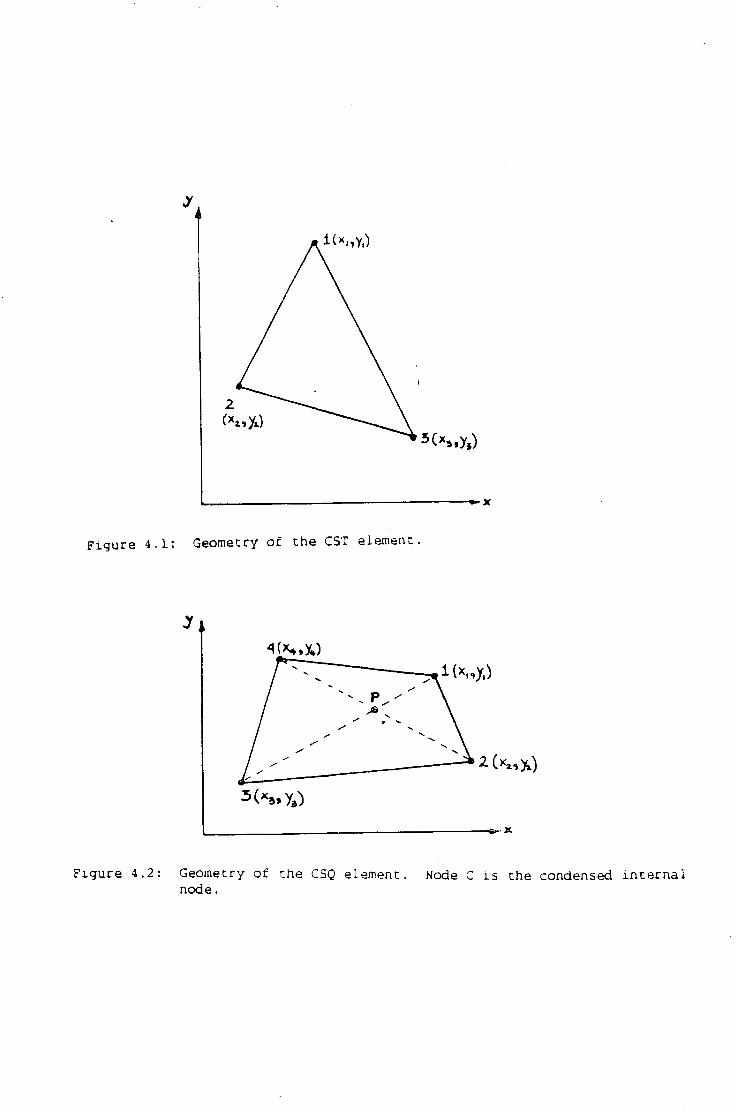
F i g u r e 4.1: Geometry o f t h e CST element
4
6»1C
F i g u r e 4.2: Geometry o f t h e CSQ elem e n t . Node C i s t h e condensed i n t e r n a l node.
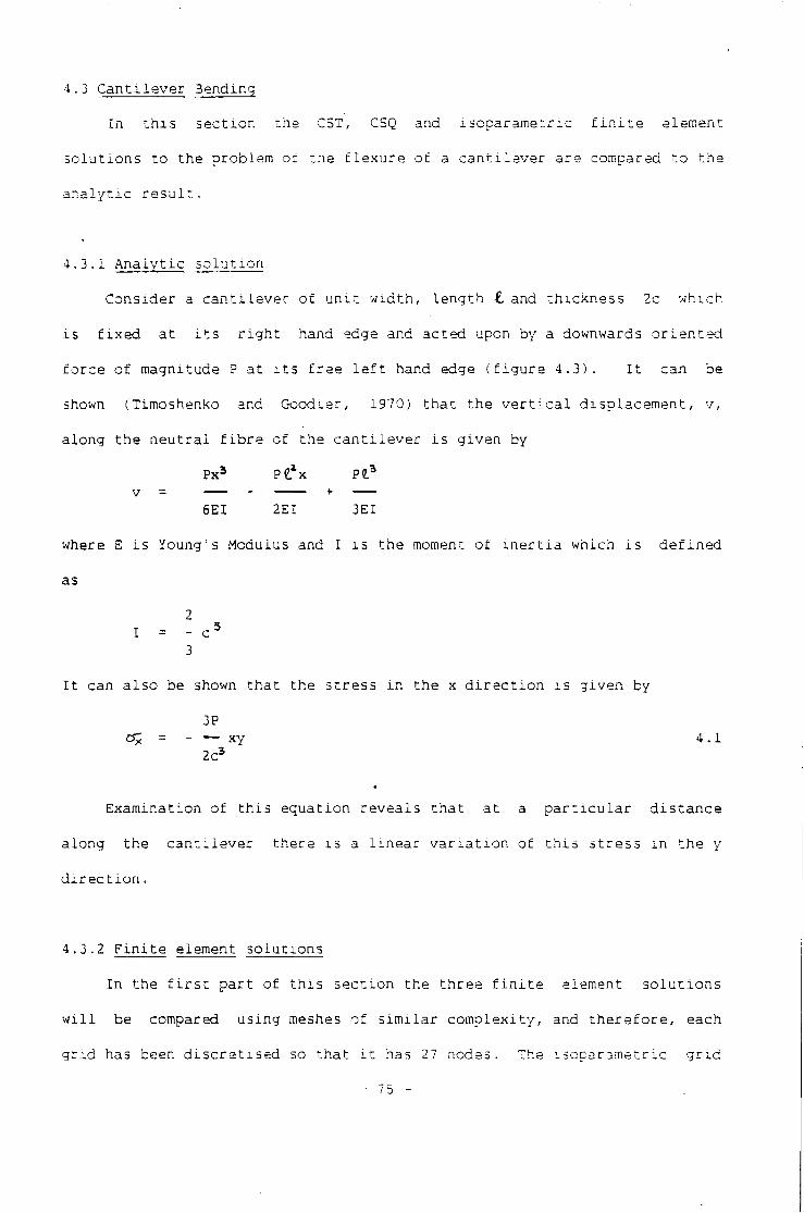
4.3 C a n t i l e v e r Bending
I n t h i s s e c t i o n t h e CST, CSQ and i s o p a r a m e t r i c f i n i t e e lement
s o l u t i o n s t o t h e p r o b l e m of t h e f l e x u r e o f a c a n t i l e v e r a r e compared t o t h e
a n a l y t i c r e s u l t .
4.3.1 A n a l y t i c s o l u t i o n
C o n s i d e r a c a n t i l e v e r o f u n i t w i d t h , l e n g t h •£, and t h i c k n e s s 2c w h i c h
i s f i x e d a t i t s r i g h t hand edge and a c t e d upon by a downwards o r i e n t e d
f o r c e o f magnitude P a t i t s f r e e l e f t hand edge ( f i g u r e 4 .3). I t can be
shown (Timoshenko and Goodi e r , 1970) t h a t t h e v e r t i c a l d i s p l a c e m e n t , v,
a l o n g t h e n e u t r a l f i b r e o f t h e c a n t i l e v e r i s g i v e n by
Px 3 P^x P I 3
6EI 2EI 3EI
where E i s Young's Modulus and I i s t h e moment o f i n e r t i a which i s d e f i n e d
as
2 I = - c 3
3
I t can a l s o be shown t h a t t h e s t r e s s i n t h e x d i r e c t i o n i s g i v e n by
3P = - — xy 4.1
2c 3
E x a m i n a t i o n o f t h i s e q u a t i o n r e v e a l s t h a t a t a p a r t i c u l a r d i s t a n c e
a l o n g t h e c a n t i l e v e r t h e r e i s a l i n e a r v a r i a t i o n o f t h i s s t r e s s i n t h e y
d i r e c t i o n .
4.3.2 F i n i t e element s o l u t i o n s
I n t h e f i r s t p a r t o f t h i s s e c t i o n t h e t h r e e f i n i t e element s o l u t i o n s
w i l l be compared u s i n g meshes o f s i m i l a r c o m p l e x i t y , and t h e r e f o r e , each
g r i d has been d i s c r e t i s e d so t h a t i t has 27 nodes. The i s o p a r a m e t r i c g r i d
- 75 -
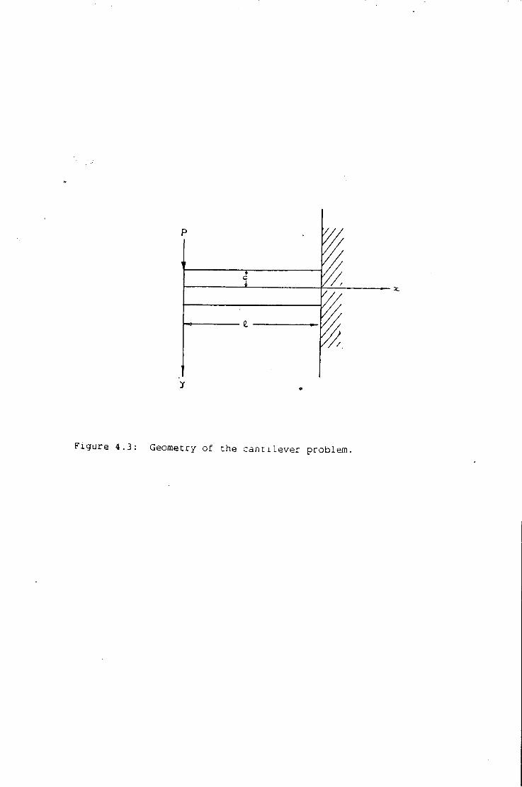
y
F i g u r e 4.3: Geometry o f t h e c a n t i l e v e r p r o b l e m .
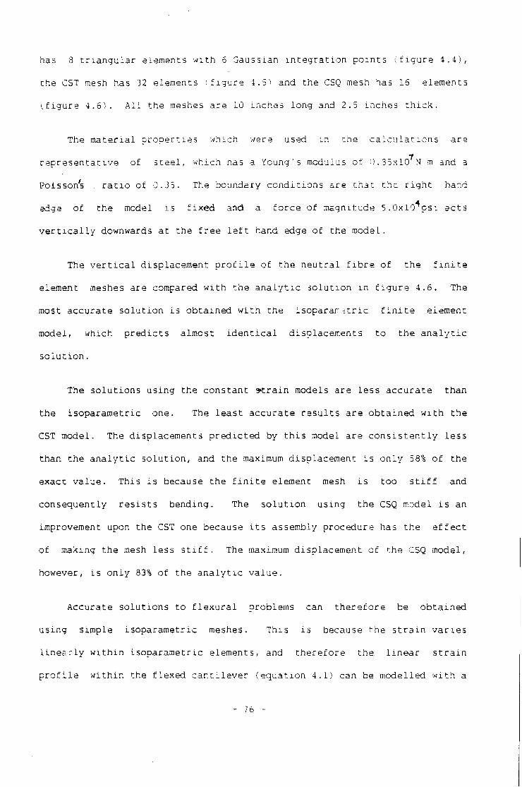
has 3 t r i a n g u l a r elements w i t h 6 Gaussian i n t e g r a t i o n p o i n t s ( f i g u r e 4 . 4 ) ,
t h e CST mesh has 32 elements ( f i g u r e 4.5) and t h e CSQ mesh has 16 e l e m e n t s
(.figure 4.6). A l l t h e meshes a r e 10 i n c h e s l o n g and 2.5 i n c h e s t h i c k .
The m a t e r i a l p r o p e r t i e s which were used i n t h e c a l c u l a t i o n s a r e
r e p r e s e n t a t i v e o f s t e e l , w h i c h has a Young's modulus of O.35xl0 TN m and a
Poisson's . r a t i o of 0.35. The boundary c o n d i t i o n s a r e chat t h e r i g h t hand
edge o f t h e model i s f i x e d and a f o r c e o f magnitude 5.0x10 p s i a c t s
v e r t i c a l l y downwards a t t h e f r e e l e f t hand edge of t h e model.
The v e r t i c a l d i s p l a c e m e n t p r o f i l e o f t h e n e u t r a l f i b r e o f t h e f i n i t e
element meshes ar e compared w i t h t h e a n a l y t i c s o l u t i o n i n f i g u r e 4.6. The
most a c c u r a t e s o l u t i o n i s o b t a i n e d w i t h t h e i s o p a r a m e t r i c f i n i t e element
model, which p r e d i c t s a l m o s t i d e n t i c a l d i s p l a c e m e n t s t o t h e a n a l y t i c
s o l u t i o n .
The s o l u t i o n s u s i n g t h e c o n s t a n t s t r a i n models a r e l e s s a c c u r a t e t h a n
t h e i s o p a r a m e t r i c one. The l e a s t a c c u r a t e r e s u l t s a r e o b t a i n e d w i t h t h e
CST model. The d i s p l a c e m e n t s p r e d i c t e d by t h i s model a r e c o n s i s t e n t l y l e s s
t h a n t h e a n a l y t i c s o l u t i o n , and t h e maximum d i s p l a c e m e n t i s o n l y 53% o f t h e
e x a c t v a l u e . T h i s i s because t h e f i n i t e element mesh i s t o o s t i f f and
c o n s e q u e n t l y r e s i s t s b e n d i n g . The s o l u t i o n u s i n g t h e CSQ model i s an
improvement upon th e CST one because i t s assembly p r o c e d u r e has t h e e f f e c t
o f making t h e mesh l e s s s t i f f . The maximum d i s p l a c e m e n t o f t h e CSQ model,
however, i s o n l y 83% o f t h e a n a l y t i c v a l u e .
A c c u r a t e s o l u t i o n s t o f l e x u r a l problems can t h e r e f o r e be o b t a i n e d
u s i n g s i m p l e i s o p a r a m e t r i c meshes. T h i s i s because t h e s t r a i n v a r i e s
l i n e a r l y w i t h i n i s o p a r a m e t r i c e l e m e n t s , and t h e r e f o r e the. l i n e a r s t r a i n
p r o f i l e w i t h i n the f l e x e d c a n t i l e v e r ( e q u a t i o n 4.1) can be m o d e l l e d w i t h a
- 76 -
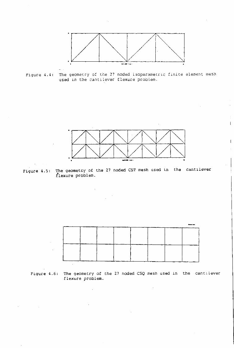
F i g u r e 4.4: The geometry o f t h e 27 noded i s o p a r a m e t r i c f i n i t e element mesh used i n t h e c a n t i l e v e r f l e x u r e p r o b l e m .
F i g u r e 4.5: The geometr.y of the 27 noded CST mesh used i n the c a n t i l e v e r f l e x u r e problem.
F i g u r e 4.6: The geometry of the 27 noded CSQ mesh used i n the c a n t i l e v e r f l e x u r e problem.
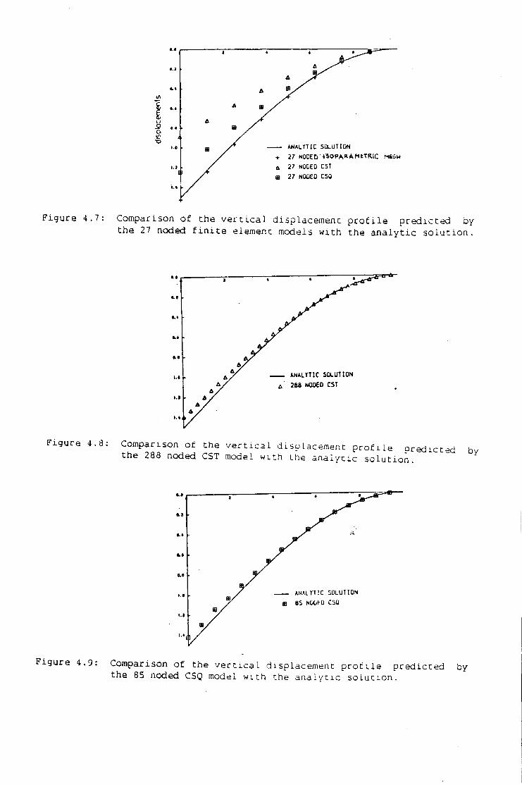
•.1
s l/l
ANALYTIC SOLUTION i.t + 27 NOOED - t S O P A ^ A M t T R I C M i S H
a 27 NCDED CST t ffl 27 NOUEO CSO
F i g u r e 4.7: Comparison o f t h e v e r t i c a l d i s p l a c e m e n t p r o f i l e p r e d i c t e d by t h e 27 noded f i n i t e element models w i t h t h e a n a l y t i c s o l u t i o n .
n
t.4
ANALYTIC SOLUTION
a 208 NODEO CST
I . I
i . « , .
F i g u r e 4.8 Comparison o f t h e v e r t i c a l d i s p l a c e m e n t p r o f i l e p r e d i c t e d by t h e 288 noded CST model w i t h t h n a l y t i c s o l u t i o n
4.6
6.8
ANALYTIC SOLUTION I . *
m ffl 85 NObt-D C5U
a I . I
F i g u r e 4.9: Comparison o f t h e v e r t i c a l d i s p l a c e m e n t p r o f i l e p r e d i c t e d by t h e 85 noded CSQ model w i t h t h e a n a l y t i c s o l u t i o n .
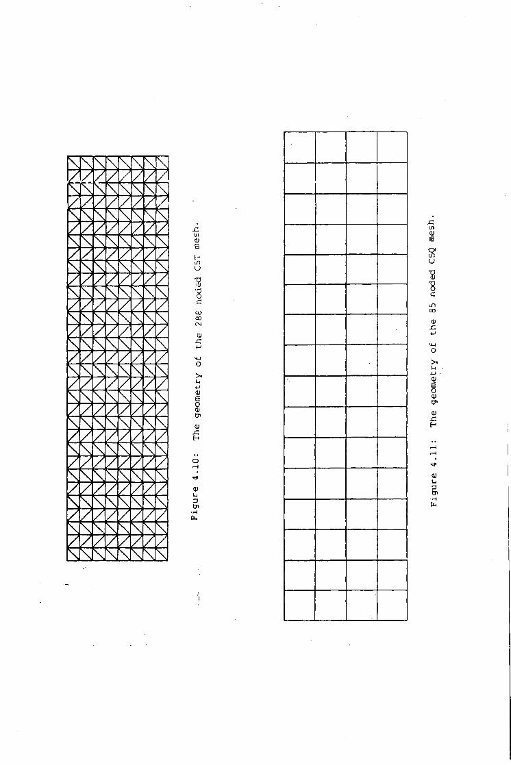
e H U "8 '8 c CO CO r-j <V -C
M 4-1 <U s o CU CP
OJ x;
o l—i
L i a 01 El4
.c 01 E O u "8 "8 in CO
ai
I * L i 4-1 -0) £ 0 ai CP
0)
u
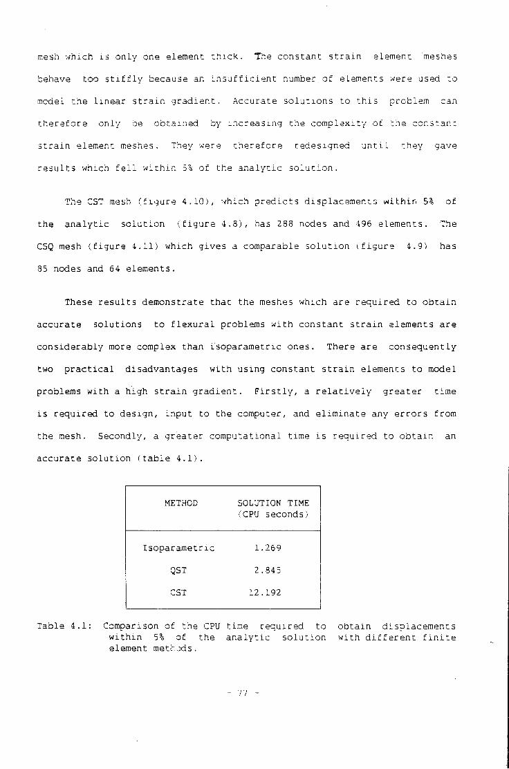
mesh whic h i s o n l y one element t h i c k . The c o n s t a n t s t r a i n element meshes
behave t o o s t i f f l y because an i n s u f f i c i e n t number.of elements were used t o
model t h e l i n e a r s t r a i n g r a d i e n t . A c c u r a t e s o l u t i o n s t o t h i s p r o b l e m can
t h e r e f o r e o n l y be o b t a i n e d by i n c r e a s i n g t h e c o m p l e x i t y o f t h e c o n s t a n t
s t r a i n element meshes. They were t h e r e f o r e r e d e s i g n e d u n t i l t h e y gave
r e s u l t s which f e l l w i t h i n 5% o f t h e a n a l y t i c s o l u t i o n .
The CST mesh ( f i g u r e 4.10), w h i c h p r e d i c t s d i s p l a c e m e n t s w i t h i n 5% o f
t h e a n a l y t i c s o l u t i o n ( f i g u r e 4 .8), has 288 nodes and 496 e l e m e n t s . The
CSQ mesh ( f i g u r e 4.11) which g i v e s a comparable s o l u t i o n ( f i g u r e 4.9) has
35 nodes and 64 e l e m e n t s .
These r e s u l t s d e m o n s t r a t e t h a t t h e meshes whic h a r e r e q u i r e d t o o b t a i n
a c c u r a t e s o l u t i o n s t o f l e x u r a l problems w i t h c o n s t a n t s t r a i n e lements a r e
c o n s i d e r a b l y more complex t h a n i s o p a r a m e t r i c ones. There a r e c o n s e q u e n t l y
two p r a c t i c a l d i s a d v a n t a g e s w i t h u s i n g c o n s t a n t s t r a i n e lements t o model
problems w i t h a h i g h s t r a i n g r a d i e n t . F i r s t l y , a r e l a t i v e l y g r e a t e r t i m e
i s r e q u i r e d t o d e s i g n , i n p u t t o t h e computer, and e l i m i n a t e any e r r o r s f r o m
t h e mesh. Secondly, a g r e a t e r c o m p u t a t i o n a l t i m e i s r e q u i r e d t o o b t a i n an
a c c u r a t e s o l u t i o n ( t a b l e 4 . 1 ) .
METHOD SOLUTION TIME (CPU seconds)
I s o p a r a m e t r i c 1.269
QST 2.345
CST 12.192
Ta b l e 4.1: Comparison o f t h e CPU t i m e r e q u i r e d t o o b t a i n d i s p l a c e m e n t s w i t h i n 5% o f t h e a n a l y t i c s o l u t i o n w i t h d i f f e r e n t f i n i t e element methods.
There i s , however, a more i m p o r t a n t d i s a d v a n t a g e i n u s i n g t h e c o n s t a n t
s t r a i n element t o model l i t h o s p h e r i c s t r e s s r e g i m e s . T h i s i s t h a t we can
o n l y be sure t h e model i s g i v i n g an a c c u r a t e s o l u t i o n by i t e r a t i v e l y
r e d e s i g n i n g t h e mesh u n t i l c o n v e r g e n t s o l u t i o n s a r e o b t a i n e d . T h i s
p r o c e d u r e , however, i s r a r e l y adopted i n p r a c t i s e because i t i s v e r y t i m e
consuming. I t i s t h e r e f o r e always p o s s i b l e t h a t c o n s t a n t s t r a i n models
w i l l a c t t o o s t i f f l y .
I t i s c o n s e q u e n t l y d e s i r a b l e t o use t h e i s o p a r a m e t r i c f i n i t e element
method t o model complex l i t h o s p h e r i c s t r e s s d i s t r i b u t i o n s because i t g i v e s
a c c u r a t e r e s u l t s w i t h a r e l a t i v e l y s i m p l e mesh d e s i g n .
4 . 4 Body Forces
The s t r e s s e s i n t h e l i t h o s p h e r e r e s u l t i n g f r o m t h e a c t i o n o f body
f o r c e s a r e g e n e r a l l y o f g r e a t e r magnitude t h a n t h o s e f r o m o t h e r s o u r c e s .
I t i s t h e r e f o r e i m p o r t a n t t h a t t h e f i n i t e element method w h i c h i s a d o p t e d
can a c c u r a t e l y model t h e s e s t r e s s e s .
I n t h i s s e c t i o n t h e s o l u t i o n s u s i n g t h e t h r e e f i n i t e element methods
a r e compared w i t h t h e a n a l y t i c s o l u t i o n f o r t h e p r o b l e m o f body f o r c e s
a c t i n g upon a f l a t c o n s t r a i n e d r e g i o n .
4.4.1 A n a l y t i c s o l u t i o n
Consider a f l a t r e g i o n , c o n s t r a i n e d f o r z e r o h o r i z o n t a l d i s p l a c e m e n t ,
of u n i f o r m d e n s i t y , p , a c t e d upon by g r a v i t y , g. Because t h e r e i s no
h o r i z o n t a l d i s p l a c e m e n t anywhere i n t h e body t h e s t r a i n , i n t h e x d i r e c t i o n
i s z e r o , i . e .
e x = o
- 78 -
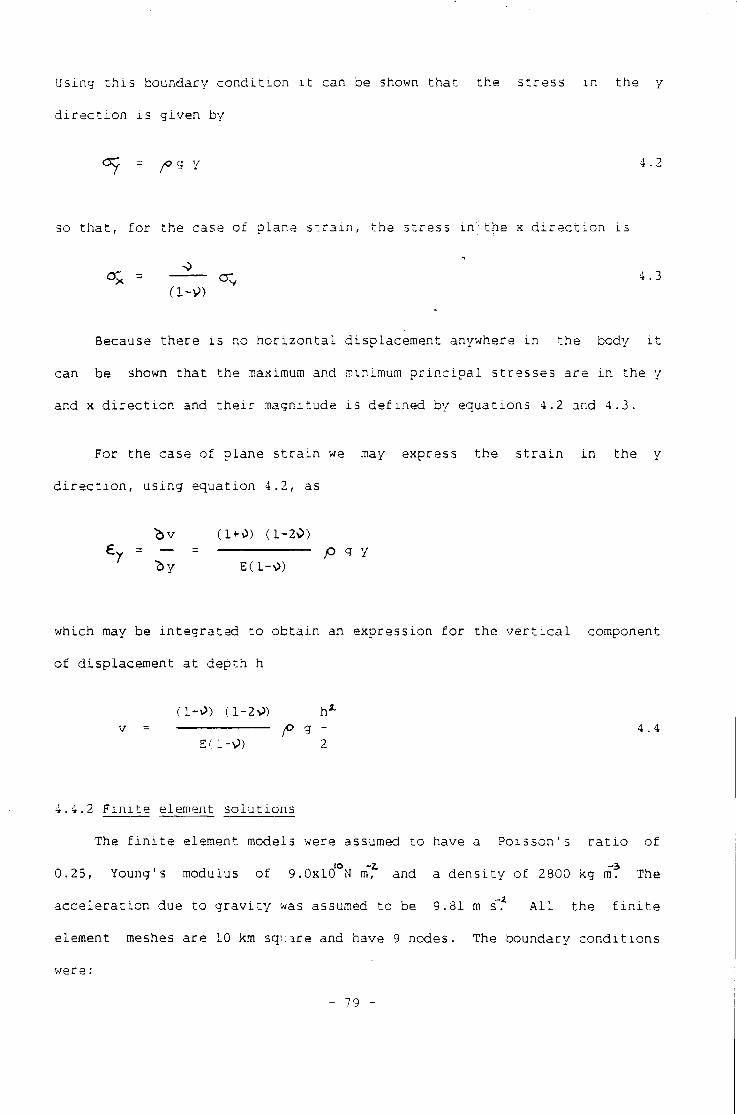
Using t h i s boundary c o n d i t i o n i t can be shown t h a t t h e s t r e s s i n t h e y
d i r e c t i o n i s g i v e n by
<3y = y 4.2
so t h a t , f o r t h e case o f p l a n e s t r a i n , t h e s t r e s s i n • t h e x d i r e c t i o n i ;
_2_ a - \ »
°; = crv 4.3
Because t h e r e i s no h o r i z o n t a l d i s p l a c e m e n t anywhere i n t h e body i t
can be shown t h a t t h e maximum and minimum p r i n c i p a l s t r e s s e s a r e m t h e y
and x d i r e c t i o n and t h e i r magnitude i s d e f i n e d by e q u a t i o n s 4.2 and 4.3.
For t h e case o f p l a n e s t r a i n we may express t h e s t r a i n i n t h e y
d i r e c t i o n , u s i n g e q u a t i o n 4.2, as
b v ( 1 + 0) (l-2v>) £y = — = — p g y
"by E(l->»
which may be i n t e g r a t e d t o o b t a i n an
o f d i s p l a c e m e n t a t d e p t h h
<l+v>) (1-20) h A
v = jO g -E(l-v>) 2
e x p r e s s i o n f o r t h e v e r t i c a l component
4 . 4
4.4.2 F i n i t e element s o l u t i o n s
The f i n i t e element models were assumed t o have a Poi s s o n ' s r a t i o o f
0.25, Young's modulus o f 9.0xlo'°N mf" and a d e n s i t y o f 2800 kg mf The
a c c e l e r a t i o n due t o g r a v i t y was assumed t o be 9.81 m s".2 A l l t h e f i n i t e
element meshes a r e 10 km square and have 9 nodes. The boundary c o n d i t i o n s
wer e:
- 79 -
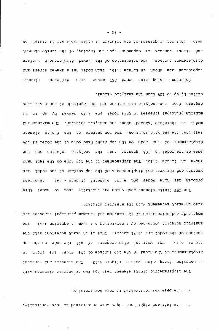
- 0 8 -
Aq pesneo EX pus e ^ q t j x s a p u n EX uoirrnxos aq3 30 ssauanbxun uou s i q j , •qseu: 3U3UI3X© a3xuxx eU3 JO A6oxodo3 sq3 uodn }UBpuadap sx SJOUDBA ssaJ3S puB B D B j j n s 3UBureDBxdsxp pa^a^E aq3 30 u o i a B i u a T j o a m -eoegjns 3uaujaoBxdsxp puB SSBJ3S pswa^s B SBq "[apouj qopg ' 9X' 1> a j n 6 x 3 ux uwoqs B J P SBT6o"[odoa 3ueui3T3 4 u e j o 3 3 T p q3Tw saqsaw iSD papou BUTU 6uTsn suoT^njos
•sanjeA DT^A-[PUP aq3 UOJ3 % 0 T 03 dn Aq j a g g x p
59sse:;s esaq3 30 apn3xu6pui aq3 pue UOT3B3UBTJO OT3AXPUB aq3 1110J3 s a a j b a p
£j 03 dn Aq pawa^s osjv B J B X 3 P O U U STq3 UT s a s s e j t j s TBdtDUTjd umuiTUTui
puB uiniuTXPUJ a m •uoT^nios OT3AXPUB 3q3 3noqp , peMa>{S, 3:1033 jaq3 ST xspou 1
3uaui3ia 33111x3 aq3 30 aopgjns do3 a q i "00x30x05 ox3AXPUB 9143 ueq3 ssax
% 0 T sx x sPOi" 3U3 3° 3bpa puBq 3U6TJ do3 aq3 uo 3pou aq} 30 3U3ui3DBxdsxp
ai(3 puB uox3nxos 0X3AXBUB aq3 upq3 J 3 3 P 3 J 6 %0X ST X 3 P ° H 5U3 30 abpa
pueq 3 j a x aq3 uo apou do3 3q3 30 3U3waopxdsxp 3m ' 'ST'f' a j n b x g UT UMOqs
a j B x A P O M 3U3 7° B^EJJns do3 aq3 30 S3uaui33exdsTp x^^x3J8A ei[3 puB S J 0 3 0 3 A
S S B J I S a q i ' ( f ' T ' t 1 a j n 6 x 3 ) S3uauiex3 3qbT3 PUB sapou BUTU spq ujsxqojd
STL{3 x s P ° ^ 03 pasn Axx ?T3TUT SPM qDTqM qssui 3uaui3X3 33TUT3 I S D aqx
' UOT3 nXOS OX 3AX BUB aU;3 q3TM 3UBUUaaj6B 30BX3 ux OSXP
BJB S3SS3J3S X p d T : ) U T : r d UintL'TUTU] pUB UinUIXKBUJ BU3 J O UOX3P3UBXJO puB 3pn3TU6BUJ
s m ' ( f t uoT3Bnbs UT uiiiOT = q £>ux3n3T3sqns Aq p3UXB3qo) uoj3nxos 0T3AXPUP
3L[3 q3XK 3uauj3aj6p 3 0 P X 3 ux sx STUJ, • saJ33UJ J L ' Z I 3 J E xepoui 3U3 ?o aoegjns
U03 au3 uo sspou aq") XT'? 3° S3uauiaoBxdsxp X e : ; t 3 J 3 A sqx 'CT't- 3.106x3
ux u.icq; e j p -apouj sua 30 eopgjns 003 eq3 uu sapou eq; 30 E3uaur3 0PT,dsTp
XB0X3ja / i pup sassaj3S . a q i '(ZT'f BJHDxg'; s3uxod UOT3PJ6B3UT uBTSsnpo 9
U 3 X A'. E 3 UBUJB X S JBxn6UBXJ"4 OM3 S Bq USBUJ 3U3UI9X3 B 4 TUT 3 OX J33UIB JBdOE T 3qX
• A x x E 3 u o z x j o q BAOUJ 03 P S U T P J 3 S U O O sew sspq aqx
•AXXEOX3J3A BAOui 03 P3UXBJ3SUOO BJBM ssbpa pueq 3q£xj puB 333x a q i 'X
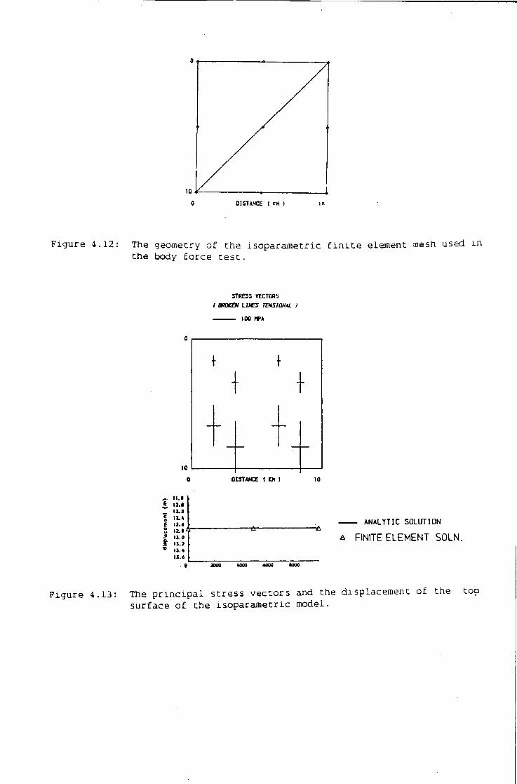
MSTA.NCE I rM )
F i g u r e 4.12: The geometry of the i s o p a r a m e t r i c f i n i t e element mesh used i n the body f o r c e t e s t .
STRESS VICTORS ( BROKBt UAE5 TdHSlQNAL )
100 M>A
DISTANCE t KH )
I I . * 1J.S ia.3 I I . * 13.*
11.0 13.J ' J *
ANALYTIC SOLUTION
A FINITE ELEMENT SOLN.
F i g u r e 4.13: The p r i n c i p a l s t r e s s v e c t o r s and the displacement of the top s u r f a c e of the i s o p a r a m e t r i c model.
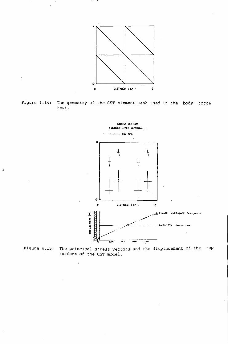
0
10
\ \ \ \1
0 OlSTANCt I th i 10
F i g u r e 4.14: The geometry o f t h e CST element mesh used i n t h e body f o r c e t e s t .
STRESS VECTORS ( BfXKEN LIKES T&G1IWAL J
100 HPA
01STANCE ( Ol )
? I I : S it.* 13.0 U.2 I I . * I3.» 13.0 I I . J IJ.» 11.4 l l .« .
' a
F i u i T t £LEHet<T ba_orvoAJ
woo 4000 caw
F i g u r e 4.15: The p r i n c i p a l s t r e s s v e c t o r s and t h e d i s p l a c e m e n t o f t h e t o p s u r f a c e o f t h e CST model.
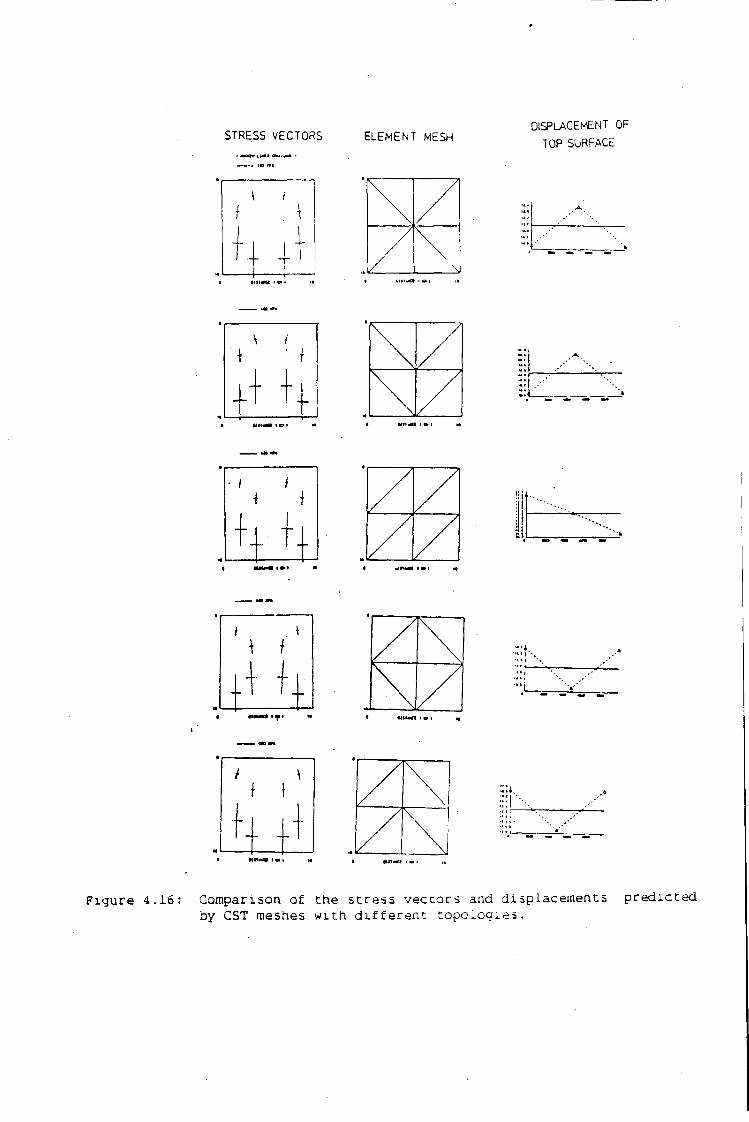
DISPLACEMENT OF S T R E S S V E C T O R S E L E M E N T MESH TOP SURFACE
H U M O I
7 /
T I
T T
l o w
F i g u r e 4.16: Comparison o f t h e s t r e s s v e c t o r s and d i s p l a c e m e n t s p r e d i c t e d by CST meshes w i t h d i f f e r e n t t o p o l o g i e s .
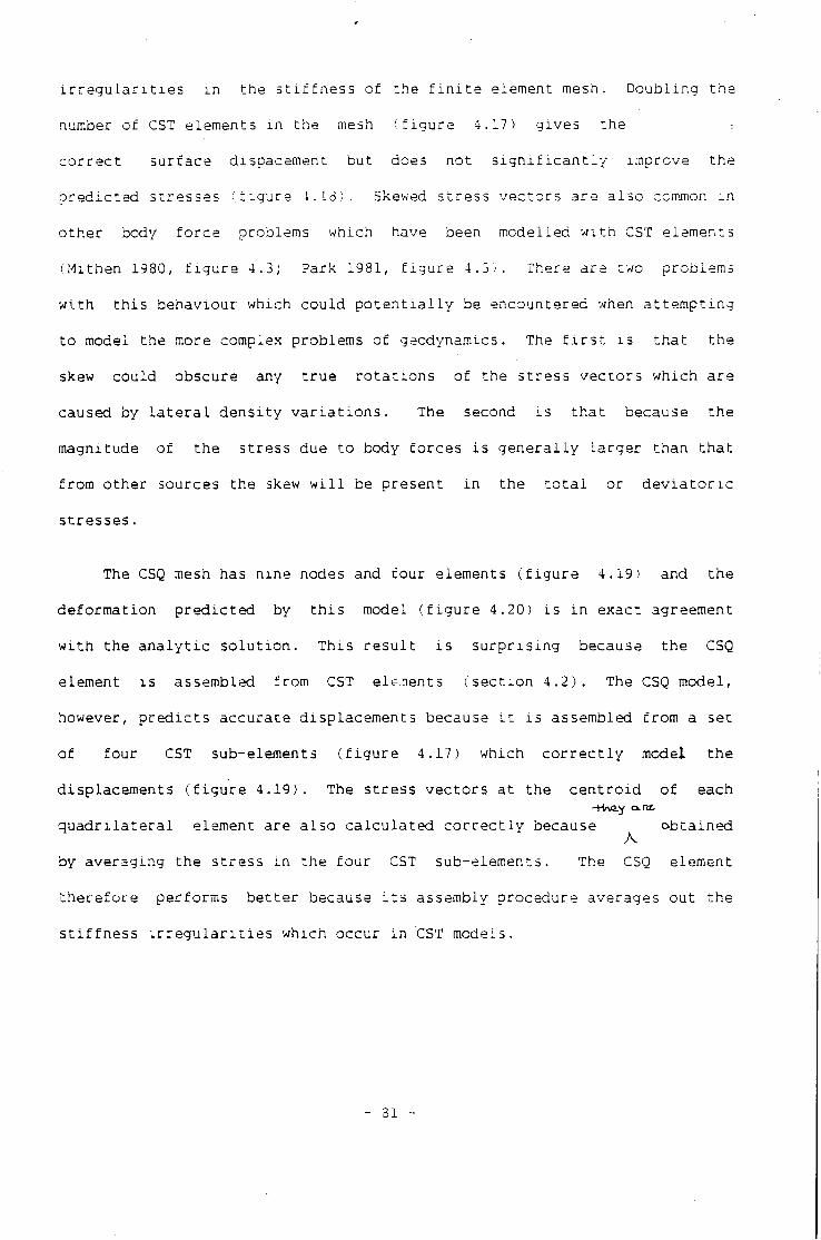
i r r e g u l a r i t i e s i n t h e s t i f f n e s s o f t h e f i n i t e element mesh. D o u b l i n g t h e
number o f CST elements i n t h e mesh ( f i g u r e 4.17) g i v e s t h e -.
c o r r e c t s u r f a c e dispacement bu t does n o t s i g n i f i c a n t l y i m p rove t h e
p r e d i c t e d s t r e s s e s ( f i g u r e 4.13'). Skewed s t r e s s v e c t o r s a r e a l s o common i n
o t h e r body f o r c e problems which have been m o d e l l e d w i t h CST e l e m e n t s
i M i t h e n 1980, f i g u r e 4.3; Park 1981, f i g u r e 4.5). There a r e two problems
w i t h t h i s b e h a v i o u r which c o u l d p o t e n t i a l l y be e n c o u n t e r e d when a t t e m p t i n g
t o model t h e more complex problems o f gecdynamics. The f i r s t i s t h a t t h e
skew c o u l d o b s c u r e any t r u e r o t a t i o n s o f t h e s t r e s s v e c t o r s w h i c h a r e
caused by l a t e r a l d e n s i t y v a r i a t i o n s . The second i s t h a t because t h e
magnitude o f t h e s t r e s s due t o body f o r c e s i s g e n e r a l l y l a r g e r t h a n t h a t
f r o m o t h e r sources t h e skew w i l l be p r e s e n t i n t h e t o t a l or d e v i a t o r i c
s t r e s s e s .
The CSQ mesh has n i n e nodes and f o u r elements ( f i g u r e 4.19) and t h e
d e f o r m a t i o n p r e d i c t e d by t h i s model ( f i g u r e 4.20) i s i n e x a c t agreement
w i t h t h e a n a l y t i c s o l u t i o n . T h i s r e s u l t i s s u r p r i s i n g because t h e CSQ
element i s assembled f r o m CST elements ( s e c t i o n 4 . 2 ) . The CSQ model,
however, p r e d i c t s a c c u r a t e d i s p l a c e m e n t s because i t i s assembled f r o m a s e t
o f f o u r CST sub-elements ( f i g u r e 4.17) which c o r r e c t l y model t h e
d i s p l a c e m e n t s ( f i g u r e 4.19). The s t r e s s v e c t o r s a t t h e c e n t r o i d o f each -H»\a.y a nz.
q u a d r i l a t e r a l element a r e a l s o c a l c u l a t e d c o r r e c t l y because o b t a i n e d
by a v e r a g i n g t h e s t r e s s i n t h e f o u r CST sub-elements. The CSO element
t h e r e f o r e p e r f o r m s b e t t e r because i t s assembly p r o c e d u r e averages o u t t h e
s t i f f n e s s i r r e g u l a r i t i e s w h i c h o c c u r i n CST models.
- 31 -
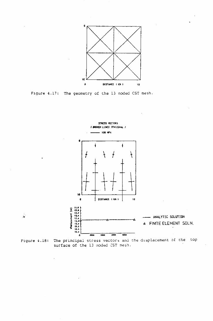
i DISTANCE < Ol 1 10
F i g u r e 4.17: The geometry o f t h e 13 noded CST mesh.
5TRE33 VECTORS 1 snaxH LIttS TTHSIONAL J
100 MPA
INSTANCE ( KM )
11. • 12. e j IX.« U.4 l l V 11.0
11.1 11.4
ANALYTIC SOLUTION
-a FINITE ELEMENT SOLN.
eooo
F i g u r e 4.18: The p r i n c i p a l s t r e s s v e c t o r s and t h e d i s p l a c e m e n t of t h e s u r f a c e o f t h e 13 noded CST mesh.
t o p
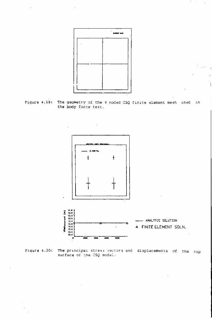
F i g u r e 4.19: The geometry of. t h e 9 noded CSQ f i n i t e e lement mesh used t h e body f o r c e t e s t .
mrmn I i ^ t m n i » u •
1.1 toe f».
T I
I I . I • 12.0 • 11.1
c o
11.» E 11.* o u ii.«Y a I
11.0 • a I 11.1 • s 11. t
ii.i
ANALYTIC SOLUTION
a FINITE ELEMENT SOLN.
F i g u r e 4.20: The p r i n c i p a l s t r e s s v e c t o r s and d i s p l a c e m e n t s o f t h e s u r f a c e o f t h e CSQ model.
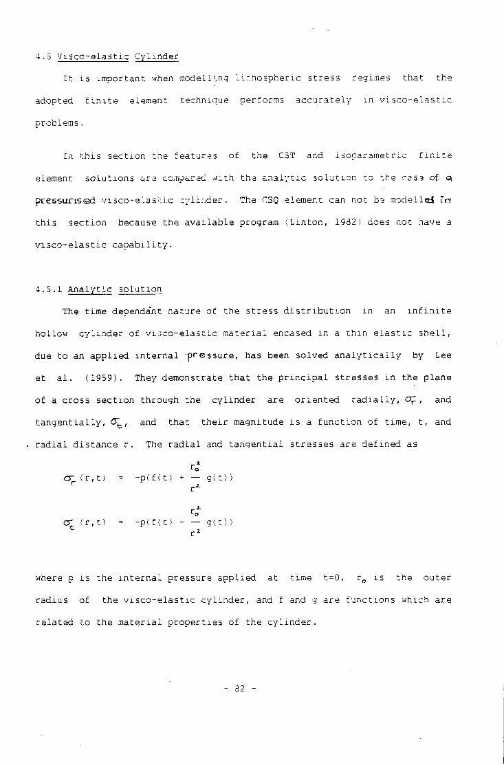
4 . 5 V i s c o - e l a s t i c C y l i n d e r
I t i s i m p o r t a n t when m o d e l l i n g l i t h o s p h e r i c s t r e s s regimes t h a t t h e
adopted f i n i t e element t e c h n i q u e p e r f o r m s a c c u r a t e l y i n v i s c o - e l a s t i c
p roblems.
I n t h i s s e c t i o n t h e f e a t u r e s o f t h e CST and i s o p a r a m e t r i c f i n i t e
element s o l u t i o n s a r e compared tii th t h e i n a l y t i c s o l u t i o n t o -.he r a s a of. a
p r e s s u r i s e d visco-e.lasci.c c y l i n d e r . The CSQ element can n o t be m o d e l l e d *r{
t h i s s e c t i o n because t h e a v a i l a b l e program ( L i n t o n , 1982) does not have a
v i s c o - e l a s t i c c a p a b i l i t y .
4.5.1 A n a l y t i c s o l u t i o n
The t i m e dependant n a t u r e o f t h e s t r e s s d i s t r i b u t i o n i n an i n f i n i t e
h o l l o w c y l i n d e r o f v i s c o - e l a s t i c m a t e r i a l encased i n a t h i n e l a s t i c s h e l l ,
due t o an a p p l i e d i n t e r n a l p r e s s u r e , has been s o l v e d a n a l y t i c a l l y by Lee
e t a l . ( 1 9 5 9 ) . They d e m o n s t r a t e t h a t t h e p r i n c i p a l s t r e s s e s i n t h e p l a n e
of a c r o s s s e c t i o n t h r o u g h t h e c y l i n d e r a r e o r i e n t e d r a d i a l l y , C£ , and
t a n g e n t i a l l y , <3J_, and t h a t t h e i r magnitude i s a f u n c t i o n o f t i m e , t , and
r a d i a l d i s t a n c e r . The r a d i a l and t a n g e n t i a l s t r e s s e s a r e d e f i n e d as
To O l ( r , t ) = - p ( f ( t ) + — g ( t ) )
r r *
c r ( r , t ) = - p ( f ( t ) g ( t ) ) * r *
where p i s t h e i n t e r n a l p r e s s u r e a p p l i e d a t t i m e t = 0 , r 0 i s t h e o u t e r
r a d i u s o f t h e v i s c o - e l a s t i c c y l i n d e r , and f and g a r e f u n c t i o n s w h i c h a r e
r e l a t e d t o t h e m a t e r i a l p r o p e r t i e s o f t h e c y l i n d e r .
- 32 -
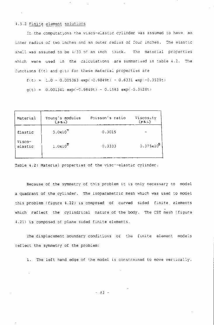
4.5.2 F i n i t e element s o l u t i o n s
I n t h e c o m p u t a t i o n s t h e v i s c o - e l a s t i c c y l i n d e r was assumed t o have an
i n n e r r a d i u s o f two i n c h e s and an o u t e r r a d i u s o f f o u r i n c h e s . The e l a s t i c
s h e l l was assumed t o be 4/33 o f an i n c h t h i c k . The m a t e r i a l p r o p e r t i e s
which were used i n t h e c a l c u l a t i o n s a r e summarised m t a b l e 4.2. The
f u n c t i o n s f ( t ) and g ( t ) f o r these m a t e r i a l p r o p e r t i e s a r e
f ( t ) = 1.0 - 0.005363 e x p ( - 0 . 9 8 4 9 t ) - 0.6331 e x p i - 0 .3523t)
g ( t ) = 0.001341 e x p ( - 0 . 9 8 4 9 t ) - 0.1583 exp(-0.3528t.)
M a t e r i a l Young's modulus Cp-3-0
Poisson's r a t i o V i s c o s i t y
E l a s t i c 3 . 0 x l 0 T 0.3015 -
V i s c o -e l a s t i c l . O x l O 5 0.3333 0.37 5 x l 0 5
T a b l e 4.2: M a t e r i a l p r o p e r t i e s o f t h e v i s e " - e l a s t i c c y l i n d e r .
Because o f t h e symmetry o f t h i s p r o b l e m i t i s o n l y n e c e s s a r y t o model
a q u a d r a n t o f t h e c y l i n d e r . The i s o p a r a m e t r i c mesh whic h was used t o model
t h i s p r o b l e m ( f i g u r e 4.22) i s composed o f c u r v e d s i d e d f i n i t e , e l ements
which r e f l e c t t h e c y l i n d r i c a l n a t u r e o f t h e body. The CST mesh ( f i g u r e
4.21) i s composed o f p l a n e s i d e d f i n i t e e l e m e n t s .
The d i s p l a c e m e n t boundary c o n d i t i o n s o f t h e f i n i t e element models
r e f l e c t t h e symmetry o f t h e p r o b l e m :
1. The l e f t hand edge o f t h e model i s c o n s t r a i n e d t o move v e r t i c a l l y .
- 33 -
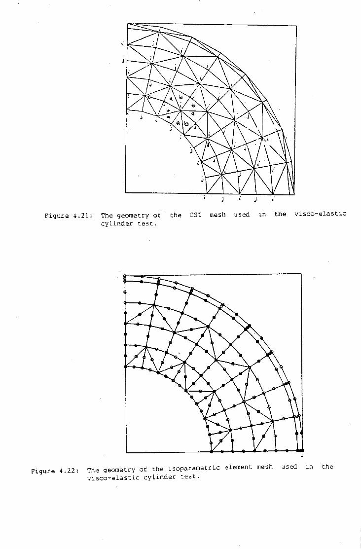
F i g u r e 4.21: The geometry o f t h e CST mesh used i n t h e v i s c o - e l a s t i c c y l i n d e r t e s t .
t h e i s o p a r a m e t r i c element mesh used i n t h e The geometry o t F i g u r e 4.22 v i s c o - e l a s t i c c y l i n d e r t e a t
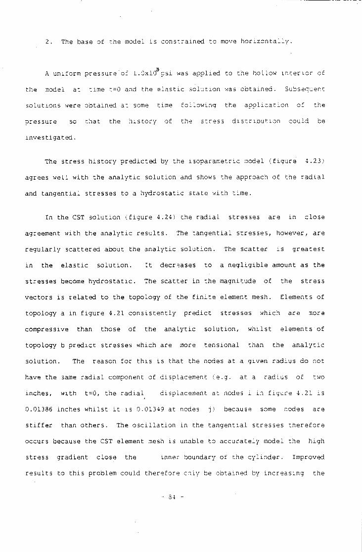
2. The base of t h e model i s c o n s t r a i n e d t o move h o r i z o n t a l l y .
3
A u n i f o r m p r e s s u r e o f i.OxlO p s i was a p p l i e d t o t h e h o l l o w i n t e r i o r o f
t h e model a t t i m e t=0 and t h e e l a s t i c s o l u t i o n was o b t a i n e d . Subsequent
s o l u t i o n s were o b t a i n e d a t some t i m e f o l l o w i n g t h e a p p l i c a t i o n o f t h e
p r e s s u r e so t h a t t h e h i s t o r y o f t h e s t r e s s d i s t r i b u t i o n c o u l d be
i n v e s t i g a t e d .
The s t r e s s h i s t o r y p r e d i c t e d by t h e i s o p a r a m e t r i c model ( f i g u r e 4.23)
agrees w e l l w i t h t h e a n a l y t i c s o l u t i o n and shows t h e approach o f t h e r a d i a l
and t a n g e n t i a l s t r e s s e s t o a h y d r o s t a t i c s t a t e w i t h t i m e .
I n t h e CST s o l u t i o n ( f i g u r e 4.24) t h e r a d i a l s t r e s s e s a r e i n c l o s e
agreement w i t h t h e a n a l y t i c r e s u l t s . The t a n g e n t i a l s t r e s s e s , however, a r e
r e g u l a r l y s c a t t e r e d about t h e a n a l y t i c s o l u t i o n . The s c a t t e r i s g r e a t e s t
i n t h e e l a s t i c s o l u t i o n . I t decreases t o a n e g l i g i b l e amount as t h e
s t r e s s e s become h y d r o s t a t i c . The s c a t t e r i n t h e magnitude o f t h e s t r e s s
v e c t o r s i s r e l a t e d t o t h e t o p o l o g y o f t h e f i n i t e element mesh. Elements o f
t o p o l o g y a i n f i g u r e 4.21 c o n s i s t e n t l y p r e d i c t s t r e s s e s w h i c h a r e more
compressive t h a n t h o s e o f t h e a n a l y t i c s o l u t i o n , w h i l s t e l e m e n t s o f
t o p o l o g y b p r e d i c t s t r e s s e s which a r e more t e n s i o n a l t h a n t h e a n a l y t i c
s o l u t i o n . The reason f o r t h i s i s t h a t t h e nodes a t a g i v e n r a d i u s do n o t
have t h e same r a d i a l component o f d i s p l a c e m e n t ( e . g . a t a r a d i u s o f two
i n c h e s , w i t h t = 0 , t h e r a d i a l d i s p l a c e m e n t a t nodes i i n f i g u r e 4.21 i s
0.01386 i n c h e s w h i l s t i t i s 0.01349 a t nodes j ) because some nodes a r e
s t i f f e r t h a n o t h e r s . The o s c i l l a t i o n i n t h e t a n g e n t i a l s t r e s s e s t h e r e f o r e
o c c u r s because t h e CST element mesh i s u n a ble t o a c c u r a t e l y model t h e h i g h
s t r e s s g r a d i e n t c l o s e t h e i n n e r boundary o f t h e c y l i n d e r . Improved
r e s u l t s t o t h i s p r o b l e m c o u l d t h e r e f o r e c n l y be o b t a i n e d by i n c r e a s i n g t h e
- 34 -
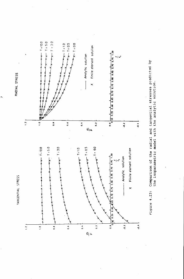
o o o b iri n — d o
o
in 1/1 L U
cr
< < cr
a
<
LU O z <
o
o c
O
c a* E
c
o o
o iri
o
3.
"8 u "9 4 u Cb c o tfl —1 0) u> VI 3 l/l a) o u 1/1
in u —4
r-t +J <fl ix —1 r-4 4-1 m c c a> a) CP c 0)
x; J-l i-j XI .c c
IT) r—1 .-t 0) T3 n) 0 u e d) u C — i *J
<u O § c o m in a 0
in (0 a. E a) O x: o
m IN
(U 1-1 •P CP
6|
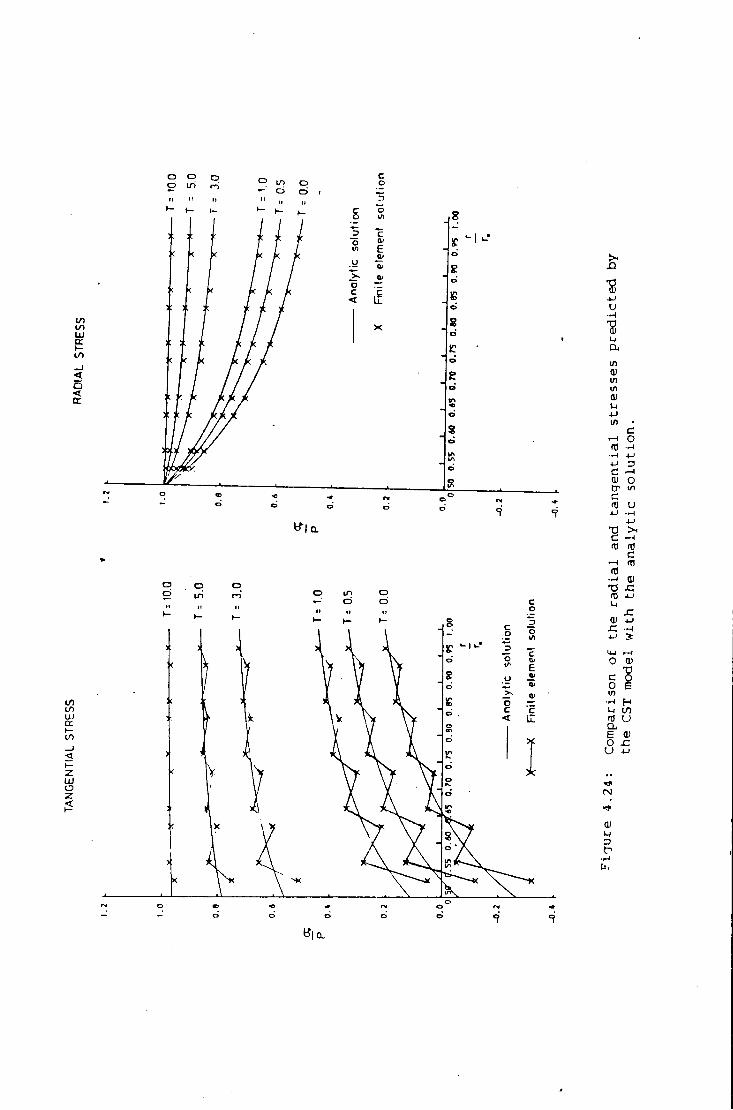
in to L U I T h-(/) < < EC
CO CO cu a: i — co _ i < t-2 L U O
10.0 o O
ro O l( H M I I
(-
o o
_3 o
D C <
c o
c a> E at c I I
o o
o iri
XI
•8 4-1 u •8 u CX
d) 10 in a) 4 J in c I—1 o m •H — i 4-1
3 c 0) o cr 1/1 c a) u j-i — I
4-J •a >s d —1
m c ~<
f0 •-i •o x: in 4_) u x: <D 4-1 r.
U-l 0
l — l d) X)
son 0
e —t H u in m u a, E 0) o JZ u 4-J
0) D
B|0L
c o m p l e x i t y o f t h e f i n i t e element mesh.
Z i e n k i e w i c z e t a l £'1963; p i o n e e r e d the a l g o r i t h m w h i c h has been used
t o model v i s c o - e l a s t i c problems i n t h i s t h e s i s . They t e s t e d t h i s a l g o r i t h m
u s i n g an i d e n t i c a l CST mesh t o the one which has been used i n t h i s s e c t i o n .
T h e i r t a n g e n t i a l s t r e s s v e c t o r s , however, agree w i t h t h e a n a l y t i c s o l u t i o n
and do noc e x h i b i t any o j c i l l a t i c n i n magnitude. D e t a i l e d c o mparison o f
t h e i r r e s u l t s w i t h t h o s e i n f i g u r e 4.24, however, shews t h a t , t h e c o r r e c t
s o l u t i o n was o b t a i n e d o n l y because t h e y averaged t h e s t r e s s i n a d j a c e n t
elements (a and b i n f i g u r e 4.21). T h e i r model t h e r e f o r e o b s c u r e s t h e t r u e
o s c i l l a t i o n i n t h e s t r e s s v e c t o r s because t h e s t i f f n e s s i r r e g u l a r i t i e s o f
th e CST mesh have been averag e d o u t .
A s i m i l a r a v e r a g i n g p r o c e d u r e has been adopted by p r e v i o u s r e s e a r c h e r s
who have m o d e l l e d t h i s t e s t case ( K u s z n i r , 1976; Woodward, 1976; M i t h e n ,
1980; Park, 1981). T h i s p r o c e d u r e , however, has n o t been a d o p t e d i n t h e i r
subsequent models, w h i c h e x p l a i n s why some o f t h e i r v i s c o - e l a s t i c s o l u t i o n s
have o s c i l l a t i n g s t r e s s v e c t o r s even a f t e r s e v e r a l m i l l i o n y e a r s r e l a x a t i o n
(e. g f i g u r e 4.13 o f Park, 1981; f i g u r e 4.4 o f M i t h e n , 1 9 8 0 ) .
I t i s t h e r e f o r e d e s i r a b l e t o adopt t h e i s o p a r a m e t r i c f i n i t e element
method t o model v i s c o - e l a s t i c s t r e s s regimes because t h i s method does n o t
e x h i b i t o s c i l l a t i o n o f t h e s t r e s s v e c t o r s .
4.6 Summary And C o n c l u s i o n s
The major r e q u i r e m e n t o f t h e f i n i t e element method w h i c h i s a d o p t e d t o
model l i t h o s p h e r i c s t r e s s regimes i s t h a t i t s h o u l d be s u f f i c i e n t l y
v e r s a t i l e t o g i v e a c c u r a t e and p r e d i c t i v e s o l u t i o n s t o a v a r i e t y o f e l a s t i c
and v i s c o - e l a s t i c p r o b l e m s .
- 35 -
I t has been shown i n t h i s c h a p t e r t h a t t h e CST element e x h i b i t s two
u n d e s i r a b l e f e a t u r e s which r e s t r i c t i t s a c c u r a c y and p r e d i c t i v e n e s s ;
1. I t behaves t o o s t i f f l y i f the mesh i s n o t o p t i m a l l y d e s i g n e d .
2. I t has a tendancy t o g i v e skewed o r o s c i l l a t i n g s t r e s s v e c t o r s i n
r e g i o n s where t h e s t r a i n g r a d i e n t i s h i g h .
The i s o p a r a m e t r i c f i n i t e element, however, p e r f o r m s a c c u r a t e l y i n e l a s t i c
and v i s c o - e l a s t i c t e s t s u s i n g r e l a t i v e l y s i m p l e meshes.
I t i s t h e r e f o r e c o n c l u d e d t h a t i t i s d e s i r a b l e t o use t h e
i s o p a r a m e t r i c f i n i t e element method t o modal l i t h o s p h e r i c s t r e s s r e g i m e s .
- 36 -
CHAPTER 5
THE ISOPARAMETRIC FINITE ELEMENT FAULT MODEL
5.1 I n t r o d u c t i o n
A f a u l t i s a p l a n e o f d i s c o n t i n u i t y a l o n g w h i c h r e l a t i v e d i s p l a c e m e n t s
have o c c u r r e d . A f a u l t o r i g i n a t e s as a f r a c t u r e p l a n e w h i c h d e v e l o p s when
t h e l i t h o s p h e r i c s t r e s s r e g i m e exceeds t h e e l a s t i c s t r e n g t h o f t h e r o c k s .
S l i p s u b s e q u e n t l y o c c u r s a l o n g t h e f r a c t u r e p l a n e . T h i s causes r e l a t i v e
d i s p l a c e m e n t s i n t h e p r e v i o u s l y c o n t i n u o u s r o c k mass and a r e d i s t r i b u t i o n
o f s t r e s s .
F o l l o w i n g t h i s p e r i o d o f i n s t a n t a n e o u s d e f o r m a t i o n t h e f a u l t e i t h e r
c o n t i n u e s t o move as a r e s u l t o f c r e e p o r i t becomes l o c k e d f o r a p e r i o d o f
t i m e , d u r i n g w h i c h s t r e s s e s a r e t r a n s m i t t e d a c r o s s t h e f a u l t p l a n e , u n t i l
t h e s t r e s s becomes l a r g e enough t o i n i t i a t e a n o t h e r p e r i o d o f i n s t a n t a n e o u s
s l i p .
C o n s e q u e n t l y , when f a u l t i n g o c c u r s a l o n g a major f a u l t p l a n e i t
m o d i f i e s t h e s t r e s s r e g i m e w h i c h e x i s t e d p r i o r t o f r a c t u r e . To b u i l d
r e a l i s t i c models o f t h e l i t h o s p h e r i c s t r e s s regime, i t i s t h e r e f o r e
n e c e s s a r y t o have a method f o r m o d e l l i n g t h e d e f o r m a t i o n a s s o c i a t e d w i t h
f a u l t s .
I n t h i s c h a p t e r a method t o model t h e f i r s t o r d e r e f f e c t s o f f a u l t i n g ,
w h i c h have been d e s c r i b e d above, i s d e v e l o p e d u s i n g t h e i s o p a r a m e t r i c
f i n i t e element method. T h i s t e c h n i q u e i s a m o d i f i c a t i o n o f t h e d u a l node
method w h i c h was d e v e l o p e d by Mi t h e n (1980) t o model f r i c t i o n a l s l i d i n g i n
c o n s t a n t s t r a i n f i n i t e e l e m e n t s . The advantage o f a f a u l t model based upon
- 37 -
t h e i s o p a r a m e t r i c f i n i t e element method i s t h a t i t a l l o w s t h e f r i c t i o n a l
s l i d i n g on c u r v e d f a u l t s t o be m o d e l l e d .
The f i r s t s e c t i o n o f t h i s c h a p t e r r e v i e w s p r e v i o u s methods which have
been proposed t o model f a u l t s u s i n g f i n i t e e l e m e n t s , f o l l o w i n g which a
method t o o b t a i n t h e s t i f f n e s s and model t h e f r i c t i c n a i s l i d i n g a l o n g t h e
f a u l t p l a n e i s d e s c r i b e d .
5.2 Review Of F i n i t e Element F a u l t Models
S e r v i c e and Douglas (1973) have suggested t h a t a f a u l t may be m o d e l l e d
i n f i n i t e element c o m p u t a t i o n s by i n t r o d u c i n g elements w i t h weak e l a s t i c
p r o p e r t i e s . M i t h e n (1980) has p o i n t e d o u t t h a t t h i s approach s u f f e r s from
two d i s a d v a n t a g e s . F i r s t l y , t h e amount by whi c h t h e e l a s t i c p a r a m e t e r s
s h o u l d be red u c e d by i s n o t known. Secondly, i t can n o t be j u s t i f i e d
t h a t a f a u l t a c t u a l l y behaves i n t h i s way. C o n s e q u e n t l y , t h i s t e c h n i q u e
w i l l n o t be used i n t h i s t h e s i s .
A s i m p l e and e f f e c t i v e method f o r i n t r o d u c i n g f a u l t s i n t o f i n i t e
element c a l c u l a t i o n s has been d e s c r i b e d by Melosh and Raefsky ( 1 9 8 1 ) . T h i s
t e c h n i q u e i s known as t h e s p l i t node t e c h n i q u e and r e q u i r e s t h a t t h e
r e l a t i v e d i s p l a c e m e n t s o f t h e nodes l y i n g on t h e f a u l t p l a n e a r e known.
These d i s p l a c e m e n t s a r e t h e n i n t r o d u c e d as p r e s c r i b e d r e l a t i v e
d i s p l a c e m e n t s by m o d i f y i n g t h e f o r c e v e c t o r . C o n s e q u e n t l y , s o l u t i o n o f t h e
s t i f f n e s s e q u a t i o n a l l o w s t h e s t r e s s e s due t o t h e p r e s c r i b e d d i s p l a c e m e n t s
t o be e v a l u a t e d .
The s p l i t node t e c h n i q u e has t h e adavantage t h a t a f a u l t can be
i n t r o d u c e d a t any node o f t h e body w i t h o u t h a v i n g t o make any a l t e r a t i o n s
t o t h e f i n i t e element mesh o r t o the s t i f f n e s s m a t r i x . The d i s a d v a n t a g e o f
th e method i s t h a t i t can n o t be used t o model t h e d e f o r m a t i o n on deep
- 38 -
f a u l t s where t h e d i s p l a c e m e n t s a r e g e n e r a l l y unknown. C o n s e q u e n t l y , t h i s
method w i l l n o t be used i n t h i s t h e s i s .
An a l t e r n a t i v e approach t o model t h e d e f o r m a t i o n a s s o c i a t e d w i t h
f a u l t i n g has been proposed by M i t h e n ( 1 9 8 0 ) , and i s known as t h e d u a l node
method. T h i s t e c h n i q u e i s an a d a p t a t i o n o f t h e method d e v e l o p e d by Goodman
e t a l (1968, t o model r e c k j o i n t s . The d u a l node method assumes t h a t t h e
l o c a t i o n o f t h e f a u l t p l a n e t s known, so t h a t i n i t i a l l y two s e p a r a t a b o d i e s
can be c o n s i d e r e d t o e x i s t t o t h e r i g h t and l e f t hand s i d e s o f t h e f a u l t
p l a n e . The f i n i t e element mesh i s t h e n d i s c r e t i s e d f o r t h e s e two b o d i e s
d u r i n g w h i c h i t i s ensured t h a t t h e nodes w h i c h f a l l on t h e f a u l t p l a n e a r e
d u a l nodes, t h a t i s , t h e y a r e formed by two nodes which a r e p r e s e n t a t t h e
same s p a t i a l l o c a t i o n s , b u t w h i c h b e l o n g t o t h e elements on o p p o s i t e s i d e s
o f t h e f a u l t p l a n e ( f i g u r e 5 . 1 ) . The s t i f f n e s s o f t h e b o d i e s on e i t h e r
s i d e o f t h e f a u l t a r e t h e n c a l c u l a t e d and i n c o r p o r a t e d i n t o t h e g l o b a l
s t i f f n e s s m a t r i x * i n t h e nor m a l way. The s t i f f n e s s m a t r i x t h e r e f o r e
c o n t a i n s t h e e l a s t i c p r o p e r t i e s o f t h e two s e p a r a t e b o d i e s and i t i s
c o n s e q u e n t l y n e c e s s a r y t o l i n k them by d e f i n i n g t h e e l a s t i c p r o p e r t i e s o f
the f a u l t . S o l u t i o n o f t h e s t i f f n e s s e q u a t i o n t h e r e f o r e y i e l d s t h e
d i s p l a c e m e n t s o f t h e f a u l t and t h e s u r r o u n d i n g m a t e r i a l under a p a r t i c u l a r
se t o f boundary c o n d i t i o n s . From t h e s e d i s p l a c e m e n t s t h e shear s t r e s s on
the f a u l t p l a n e can be c a l c u l a t e d and, i f i t i s g r e a t e r t h a n t h e f r i c t i o n a l
s t r e n g t h o f t h e f a u l t , s l i p i s a l l o w e d t o oc c u r on t h e f a u l t p l a n e u n t i l
e q u i l i b r i u m i s a c h i e v e d .
The d u a l node method i s c o m p a t i b l e w i t h t h e approach w h i c h i s t o be
ad o p t e d i n t h i s t h e s i s because i t a l l o w s t h e d i s p l a c e m e n t o f t h e f a u l t and
th e r e s u l t i n g s t r e s s e s t o be computed f o r v a r i o u s t y p e s o f boundary
c o n d i t i o n s . C o n s e q u e n t l y , t h e d u a l node method w i l l be m o d i f i e d i n t h i s
- 89 -
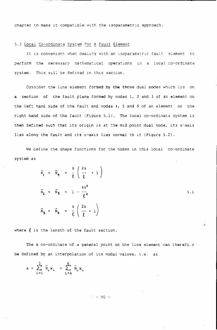
c h a p t e r t o make i t c o m p a t i b l e w i t h t h e i s o p a r a m e t r i c a p p r o a c h .
5.3 L o c a l C o - o r d i n a t e System For A F a u l t Element
I t i s c o n v e n i e n t when d e a l i n g w i t h an i s o p a r a m e t r i c f a u l t element t o
p e r f o r m t h e n e c e s s a r y m a t h e m a t i c a l o p e r a t i o n s i n a l o c a l c o - o r d i n a t e
system. T h i s w i l l be d e f i n e d i n t h i s s e c t i o n .
C o n s i d e r t h e l i n e element formed by t h e t h r e e d u a l nodes w h i c h l i e on
a s e c t i o n o f t h e f a u l t p l a n e formed by nodes 1, 2 and 3 o f an element on
t h e l e f t hand s i d e o f t h e f a u l t and nodes 4, 5 and 6 o f an element on t h e
r i g h t hand s i d e o f t h e f a u l t ( F i g u r e 5 . 1 ) . The l o c a l c o - o r d i n a t e system i s
t h e n d e f i n e d such t h a t i t s o r i g i n i s a t t h e mid p o i n t d u a l node, i t s s - a x i s
l i e s a l o n g t h e f a u l t and i t s n - a x i s l i e s normal t o i t ( F i g u r e 5 . 2 ) .
We d e f i n e t h e shape f u n c t i o n s f o r t h e nodes i n t h i s l o c a l c o - o r d i n a t e
system as
2s N N
i
4s N N
2s N N
i
5.1
where % i s t h e l e n g t h o f t h e f a u l t s e c t i o n .
The x c o - o r d i n a t e o f a g e n e r a l p o i n t on t h e l i n e element can t h e r e f o r e
be d e f i n e d by an i n t e r p o l a t i o n o f i t s n o d a l v a l u e s , i . e . as
3 6
x = H N L x u = 52 NLx-^ i = l i = 4
- 90 -

A y
s \ 4
fault plane
F i g u r e 5.1: The geometry o f t h e i s o p a r a m e t r i c f a u l t model.
F i g u r e 5.2: The l o c a l (. s,rn c o - o r d i n a t e system o f an i s o p a r a m e t r i c e l e m e n t .
f a u l t
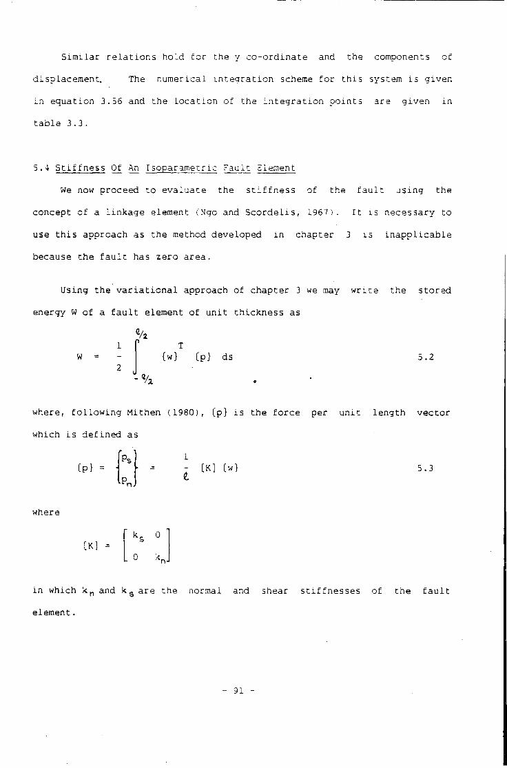
S i m i l a r r e l a t i o n s h o l d f o r the y c o - o r d i n a t e and t h e components o f
d i s p l a c e m e n t . The n u m e r i c a l i n t e g r a t i o n scheme f o r t h i s system i s g i v e n
i n e q u a t i o n 3.56 and t h e l o c a t i o n o f t h e i n t e g r a t i o n p o i n t s a r e g i v e n i n
t a b l e 3.3.
5.4 S t i f f n e s s Of An I s o p a r a m e t r i c F a u l t Element
We now p r o c e e d t o e v a l u a t e t h e s t i f f n e s s o f t h e f a u l t u s i n g t h e
c o n c e p t o f a l i n k a g e element (Ngo and S c o r d e l i s , 1967). I t i s n e c e s s a r y t o
use t h i s a p proach as t h e method d e v e l o p e d i n c h a p t e r 3 i s i n a p p l i c a b l e
because t h e f a u l t has z e r o a r e a .
U s i n g t h e v a r i a t i o n a l approach o f c h a p t e r 3 we may w r i t e t h e s t o r e d
energy W o f a f a u l t element o f u n i t t h i c k n e s s as
w = Cw} (p) ds 5.2
where, f o l l o w i n g M i t h e n ( 1 9 8 0 ) , {p} i s t h e f o r c e per u n i t l e n g t h v e c t o r
w h i c h i s d e f i n e d as
1 Cp} =
r \ p. [ K ] Cw} 5.3
where
[ K ] = k s 0
0 K
i n w h i c h k n and k s a r e t h e normal and shear s t i f f n e s s e s o f t h e f a u l t
e l e m e n t .
- 91 -
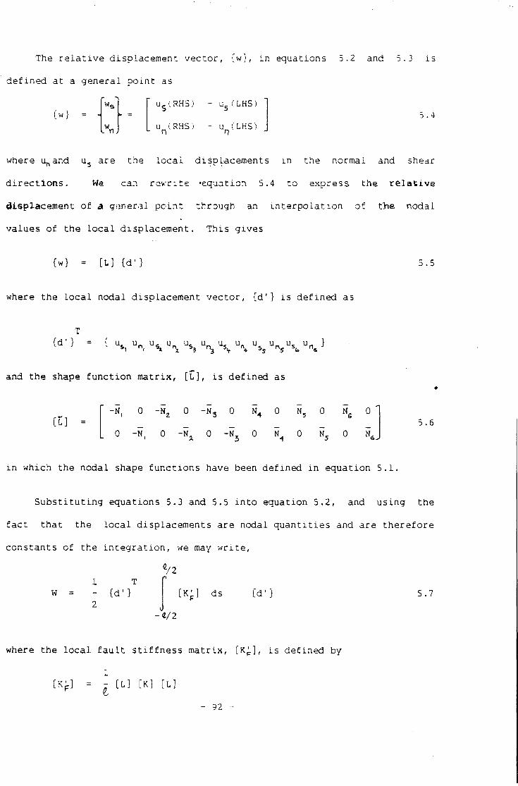
The r e l a t i v e d i s p l a c e m e n t v e c t o r , [ w ] , i n e q u a t i o n s 5.2 and 5.3 i s
d e f i n e d a t a g e n e r a l p o i n t as
fw} - =
L nj
u $(RHS) - u s(LHS)
u (RHS) - u (LHS) n n
5 . 4
where u h a n d u 5 a r e t h e . l o c a l d i s p l a c e m e n t s i n t h e normal and shear
d i r e c t i o n s . We can r e w r i t e • e q u a t i o n 5.4 t o express, t h e r e l a t i v e
d isplacement o f a g o r e r a l p o i n t t h r o u g h an i n t e r p o l a t i o n o f the n o d a l
v a l u e s o f the l o c a l d i s p l a c e m e n t . T h i s g i v e s
{w} = [ L ] ( d ' }
where t h e l o c a l n o d a l d i s p l a c e m e n t v e c t o r , ( d ' } i s d e f i n e d as
5.5
Cd' } = { u S i u n > u ^ U | v u % u ^ u n 5 u 5 f o u n s }
and the shape f u n c t i o n matrix, [ L ] , i s d e f i n e d as
[ L ] = -N, 0 -N 2 0 -N 3 0 N 4 0 N 5 0 N g 0
0 -N. 0 -Na 0 -Nj 0 0 N 5 0 N 6 J
i n w h i c h t h e n o d a l shape f u n c t i o n s have been d e f i n e d i n e q u a t i o n 5.1.
5.6
S u b s t i t u t i n g e q u a t i o n s 5.3 and 5.5 i n t o e q u a t i o n 5.2, and u s i n g t h e
f a c t t h a t t h e l o c a l d i s p l a c e m e n t s a r e n o d a l q u a n t i t i e s and a r e t h e r e f o r e
c o n s t a n t s o f t h e i n t e g r a t i o n , we may w r i t e ,
72 1 T
W = - ( d ' } 2
[ K ' j ds ( d ' } 5.7
•4/2
where t h e l o c a l f a u l t s t i f f n e s s m a t r i x , [ K ^ ] , i s d e f i n e d by
1 [Kp] = - [ L ] [K] [ L ]
- 92
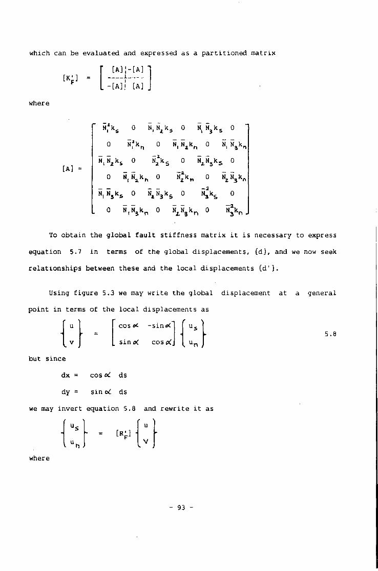
which can be evalu a t e d and expressed as a p a r t i t i o n e d matrix
where
[ A ] J - [ A ] 1
L - [ A ] ) [ A ]
t A ] =
N( k s 0 N,N zk 5 0 N tN 3k s 0
0 0 S,N ak n 0 S,S 3k n
NjNgkj 0 N*k s 0 ^ N j k s 0
0 N (N ak h 0 N X 0 N 2N 3k f t
N, N s k s 0 N xN 3k s 0 N j k s 0
0 S r S a k n 0 N ^ k , , 0 N*k„.
To o b t a i n the g l o b a l f a u l t s t i f f n e s s matrix i t i s n e c e s s a r y to express
equation 5.7 i n terms of the g l o b a l displacements, { d } , and we now seek
r e l a t i o n s h i p s between these and the l o c a l displacements { d ' } .
Using f i g u r e 5.3 we may w r i t e the g l o b a l displacement a t a ge n e r a l
p o i n t i n terms of the l o c a l displacements as
u<
v n )
u cos oC - s i n e * r =
v sino< cospCj
but s i n c e
dx = cos oC ds
dy = s i n aC ds
we may i n v e r t equation 5.8 and r e w r i t e i t as
5.8
[Rp] u
V
where
- 93 -
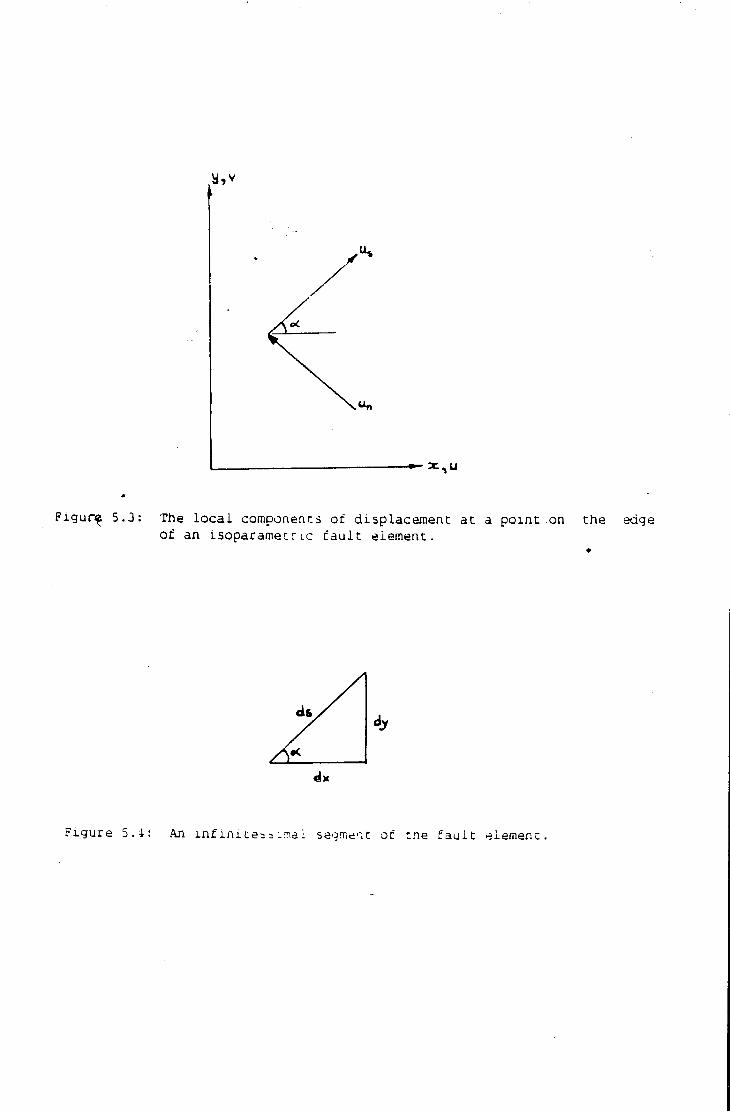
...
/
F i g u r ^ 5.3: The l o c a l components o f d i s p l a c e m e n t a t a p o i n t on t h e edge o f an i s o p a r a m e t r i c f a u l t e l ement.
as
F i g u r e 5.4: An i n f i n i c e s s . m a i segment o f t h e f a u l t element.
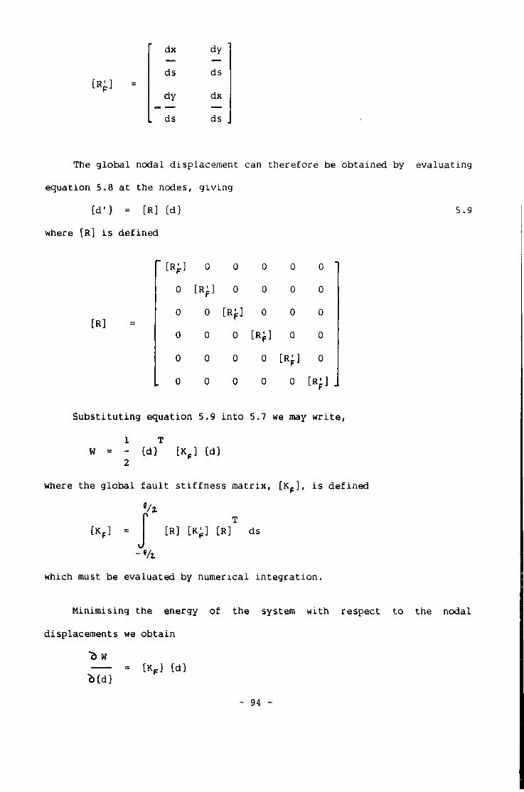
dx dy
ds ds
dy dx
ds ds
The g l o b a l nodal displacement can t h e r e f o r e be obtained by e v a l u a t i n g
equation 5.8 a t the nodes, g i v i n g
Cd 1} = [R] (d) 5.9
where [R] i s d e f i n e d
[R]
[Rp] 0 0
0 [R'] 0
0 0 0
0 0 0
0 0 [R'f] 0 0 0
0 0 0 [R'f] 0 0
0 0 0 0 [R'] 0
0 0 0 0 0 [R']
S u b s t i t u t i n g equation 5.9 i n t o 5.7 we may w r i t e ,
1 T W = - {d} [K_] {d}
2 P
where the g l o b a l f a u l t s t i f f n e s s matrix, [ K p ] , i s d e f i n e d
[ K f ] = [R] [Kp] [R] ds
which must be eval u a t e d by numerical i n t e g r a t i o n .
Minimising the energy of the system with r e s p e c t to the nodal
displacements we o b t a i n
"d W
M d } = [ K F ] ( d )
94
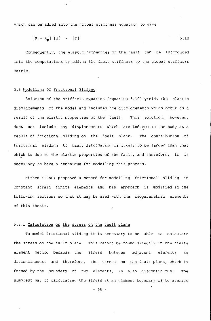
w h i c h can be added i n t o t h e g l o b a l s t i f f n e s s e q u a t i o n t o g i v e
[K + K p ] Cd} = ( F ) 5.10
C o n s e q u e n t l y , t h e e l a s t i c p r o p e r t i e s o f t h e f a u l t can be i n t r o d u c e d
i n t o t h e c o m p u t a t i o n s by a d d i n g t h e f a u l t s t i f f n e s s t o t h e g l o b a l s t i f f n e s s
m a t r i x .
5.5 M o d e l l i n g Of F r i c t i o n a l S l i d i n g
S o l u t i o n o f t h e s t i f f n e s s e q u a t i o n ( e q u a t i o n 5.10) y i e l d s t h e e l a s t i c
d i s p l a c e m e n t s o f t h e model and i n c l u d e s t h e d i s p l a c e m e n t s w h i c h o c c u r as a
r e s u l t o f t h e e l a s t i c p r o p e r t i e s o f t h e f a u l t . T h i s s o l u t i o n , however,
does n o t i n c l u d e any d i s p l a c e m e n t s w h i c h a r e i n d u c e d i n t h e body as a
r e s u l t o f f r i c t i o n a l s l i d i n g on t h e f a u l t p l a n e . The c o n t r i b u t i o n o f
f r i c t i o n a l s l i d i n g t o f a u l t d e f o r m a t i o n i s l i k e l y t o be l a r g e r t h a n t h a t
w h i c h i s due t o t h e e l a s t i c p r o p e r t i e s o f t h e f a u l t , and t h e r e f o r e , i t i s
n e c e s s a r y t o have a t e c h n i q u e f o r m o d e l l i n g t h i s p r o c e s s .
M i t h e n (1980) proposed a method f o r m o d e l l i n g f r i c t i o n a l s l i d i n g i n
c o n s t a n t s t r a i n f i n i t e e lements and h i s approach i s m o d i f i e d i n t h e
f o l l o w i n g s e c t i o n s so t h a t i t may be used w i t h t h e i s o p a r a m e t r i c elements
o f t h i s t h e s i s .
5.5.1 C a l c u l a t i o n o f t h e s t r e s s on t h e f a u l t p l a n e
To model f r i c t i o n a l s l i d i n g i t i s n e c e s sary t o be a b l e t o c a l c u l a t e
t h e s t r e s s on t h e f a u l t p l a n e . T h i s cannot be f o u n d d i r e c t l y i n t h e f i n i t e
element method because t h e s t r e s s between a d j a c e n t elements i s
d i s c o n t i n u o u s , and t h e r e f o r e , t h e s t r e s s on t h e f a u l t p l a n e , w h i c h i s
formed by t h e boundary o f two elements, i s a l s o d i s c o n t i n u o u s . The
s i m p l e s t way o f c a l c u l a t i n g t h e s t r e s s a t an element boundary i s t o average
- 95 -
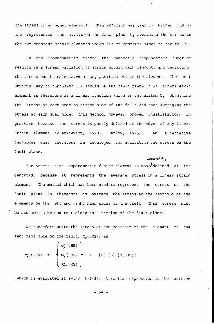
t h e s t r e s s i n a d j a c e n t e l e m e n t s . T h i s approach was used by M i t h e n (1980)
who r e p r e s e n t e d t h e s t r e s s on t h e f a u l t p l a n e by a v e r a g i n g t h e s t r e s s i n
t h e two c o n s t a n t s t r a i n elements w h i c h l i e on o p p o s i t e s i d e s o f t h e f a u l t .
I n t h e i s o p a r a m e t r i c method t h e q u a d r a t i c d i s p l a c e m e n t f u n c t i o n
r e s u l t s i n a l i n e a r v a r i a t i o n of s t r a i n w i t h i n each element, and t h e r e f o r e ,
che a t r e s s can be c a l c u l a t e d a t any p o s i t i o n w i t h i n t h e e lement. The most
o b v i o u s way t o r e p r e s e n t s t r e s s on t h e f a u l t p l a n e i n an i s o p a r a m e t r i c
element i s t h e r e f o r e as a l i n e a r f u n c t i o n w h i c h i s c a l c u l a t e d by o b t a i n i n g
t h e s t r e s s a t each node on e i t h e r s i d e o f t h e f a u l t and t h e n a v e r a g i n g t h e
s t r e s s a t each d u a l node. T h i s method, however, p r o v e d u n s a t i s f a c t o r y i n
p r a c t i s e because t h e s t r e s s i s p o o r l y d e f i n e d a t t h e edges o f any l i n e a r
s t r a i n element ( Z i e n k i e w i c z , 1979; B arlow, 1976). An a l t e r n a t i v e
t e c h n i q u e must t h e r e f o r e be d e v e l o p e d f o r e v a l u a t i n g t h e s t r e s s on t h e
f a u l t p l a n e .
The s t r e s s i n an i s o p a r a m e t r i c f i n i t e element i s m o s t / d e f i n e d a t i t s
c e n t r o i d , because i t r e p r e s e n t s t h e average s t r e s s i n a l i n e a r s t r a i n
e l e ment. The method wh i c h has been used t o r e p r e s e n t t h e s t r e s s on t h e
f a u l t p l a n e i s t h e r e f o r e t o average t h e s t r e s s a t t h e c e n t r o i d o f t h e
elements on t h e l e f t and r i g h t hand s i d e s o f t h e f a u l t . T h i s s t r e s s must
be assumed t o be c o n s t a n t a l o n g t h i s s e c t i o n o f t h e f a u l t p l a n e .
We t h e r e f o r e w r i t e t h e s t r e s s a t t h e c e n t r o i d o f t h e element on t h e
l e f t hand s i d e o f t h e f a u l t , 0~(LHS), as
( w h i c h i s e v a l u a t e d a t s = l / 3 , t = l / 3 ) . A s i m i l a r e x p r e s s i o n can be w r i t t e n
aCCurat«U*
d e f i n
c r(LHS)
c r (LHS) = c r ( L H S ) "
^x/LHS) _
[C] [ B ] ( d ( L H S ) }
- 96 -

f o r t h e s t r e s s a t t h e c e n t r o i d o f t h e element on t h e r i g h t hand s i d e o f t h e
f a u l t p l a n e , <3^(RHS). We may t h e r e f o r e w r i t e t h e s t r e s s on t h e f a u l t
p l a n e , ( ^ j , as t h e average o f t h e s e components
Co;} =
<S;(LHS) + o"^(RHS)
= - i <rY(LHS) - o^(RHS) -
We can now _ i n d e x p r e s s i o n s f o r t h e normal ? t r e s s , C , and shear
s t r e s s , £ , on t h e f a u l t p l a n e
0~ - <T^ cos*© + <Ty s i n * 6 + 2 t J ^ c o s 0 sin©
t = ( i g - O " ) s i n 0 c o s 6 + ^ ( c o s ^ S - sin2"© )
where 0 i s the hade of the f a u l t and i s d e f i n e d
a r c t a n \- — dx
dy
where
dx
dy
dx
ds
dy
ds
d H N
ds
ds
5.11
w h i c h i s e v a l u a t e d a t t h e m i d p o i n t d u a l node on t h e f a u l t segment as t h i s
r e p r e s e n t s t h e average hade o f t h e f a u l t element.
I f body f o r c e s have n o t been i n c l u d e d i n t h e model i t i s n e c e s s a r y t o
m o d i f y t h e normal s t r e s s component 3 and f o r a l i t h o s t a t i c s t r e s s
d i s t r i b u t i o n t h i s may be w r i t t e n
<r = <r+ pq Y m
where i s t h e d e n s i t y , g i s t h e a c c e l e r a t i o n due t o g r a v i t y and y m i s t h e
- 97
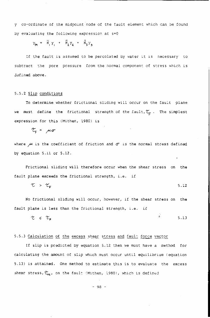
y c o - o r d i n a t e o f t h e m i d p o i n t node of t h e f a u l t element w h i c h can be f o u n d
by e v a l u a t i n g t h e f o l l o w i n g e x p r e s s i o n a t s=0
Y_ = N y + N„ y, + N, y
I f t h e f a u l t i s assumed t o be p e r c o l a t e d by water i t i s n e c e s s a r y t o
s u b t r a c t t h e p o r e p r e s s u r e f r o m t h e normal component o f s t r e s s w h i c h i s
d e f i n e d above.
5.5.2 S l i p c o n d i t i o n s
To d e t e r m i n e whether f r i c t i o n a l s l i d i n g w i l l o c c u r on t h e f a u l t p l a n e
we must d e f i n e t h e f r i c t i o n a l s t r e n g t h o f t h e f a u l t , X.^. . The s i m p l e s t
e x p r e s s i o n f o r t h i s ( M i t h e n , 1980) i s
f p = / u c r
where yU i s t h e c o e f f i c i e n t o f f r i c t i o n and C~ i s t h e normal s t r e s s d e f i n e d
by e q u a t i o n 5.11 o r 5.12.
F r i c t i o n a l s l i d i n g w i l l t h e r e f o r e o c c u r when t h e shear s t r e s s on t h e
f a u l t p l a n e exceeds t h e f r i c t i o n a l s t r e n g t h , i . e . i f
K > X? 5.12
No f r i c t i o n a l s l i d i n g w i l l o c c u r , however, i f t h e shear s t r e s s on t h e
f a u l t p l a n e i s l e s s t h a n t h e f r i c t i o n a l s t r e n g t h , i . e . i f
t $ r F - 5 . 1 3
5.5.3 C a l c u l a t i o n o f t h e excess shear s t r e s s and f a u l t f o r c e v e c t o r
I f s l i p i s p r e d i c t e d by e q u a t i o n 5.12 t h e n we must have a method f o r
c a l c u l a t i n g t h e amount o f s l i p w hich must occur u n t i l e q u i l i b r i u m ( e q u a t i o n
5.13) i s a t t a i n e d . One method t o e s t i m a t e t h i s i s t o e v a l u a t e t h e excess
shear s t r e s s , ^ , on t h e f a u l t ( M i t h e n , 1980), which i s d e f i n e d
- 98 -
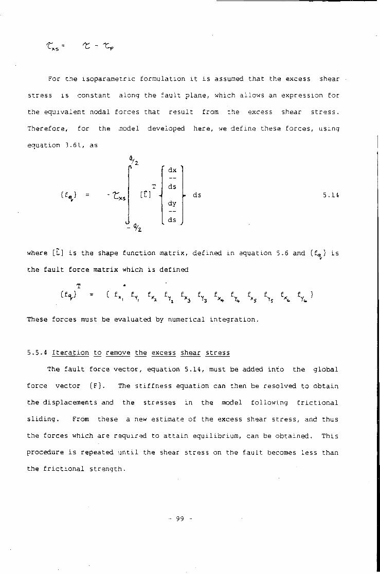
For t h e i s o p a r a m e t r i c f o r m u l a t i o n i t i s assumed t h a t t h e excess shear
s t r e s s i s c o n s t a n t a l o n g t h e f a u l t p l a n e , w h i c h a l l o w s an e x p r e s s i o n f o r
t h e e q u i v a l e n t n o d a l f o r c e s t h a t r e s u l t f r o m t h e excess shear s t r e s s .
T h e r e f o r e , f o r t h e model d e v e l o p e d h e r e , we d e f i n e t h e s e f o r c e s , u s i n g
e q u a t i o n 3.61, as
1 ' dx '
T ds [ L ] . -
dy -
dy
ds
ds 5 .14
where [ L ] i s t h e shape f u n c t i o n m a t r i x , d e f i n e d i n e q u a t i o n 5.6 and {f<^} i s
t h e f a u l t f o r c e m a t r i x w h i c h i s d e f i n e d
C f ~ f„ f« f. f.. f x, -y, ^ ^ -Y3 X X % S, fxfc fyfc
] C f ^ } = C fw f
These f o r c e s must be e v a l u a t e d by n u m e r i c a l i n t e g r a t i o n .
5.5.4 I t e r a t i o n t o remove t h e excess shear s t r e s s
The f a u l t f o r c e v e c t o r , e q u a t i o n 5.14, must be added i n t o t h e g l o b a l
f o r c e v e c t o r ( F } . The s t i f f n e s s e q u a t i o n can t h e n be r e s o l v e d t o o b t a i n
t h e d i s p l a c e m e n t s and t h e s t r e s s e s i n t h e model f o l l o w i n g f r i c t i o n a l
s l i d i n g . From these a new e s t i m a t e o f t h e excess shear s t r e s s , and t h u s
t h e f o r c e s w h i c h a r e r e q u i r e d t o a t t a i n e q u i l i b r i u m , can be o b t a i n e d . T h i s
p r o c e d u r e i s r e p e a t e d u n t i l t h e shear s t r e s s on t h e f a u l t becomes l e s s t h a n
t h e f r i c t i o n a l s t r e n g t h .
- 99 -
CHAPTER 6
FRICTIONAL SLIDING ON PLANE AND LISTRIC FAULTS
I n t h i s c h a p t e r t h e i s o p a r a m e t r i c f a u l t model ( c h a p t e r 5) i s used t o
a n a l y s e t h e d e f o r m a t i o n w h i c n r e s u l t s from f r i c t i o n a l s l i d i n g on p l a n e and
l i s t r i c f a u l t s .
There a r e t h r e e aims t o t h i s c h a p t e r . The f i r s t i s t o examine t h e
c h a r a c t e r i s t i c s o f t h e model by e x a m i n i n g i t s response t o f r i c t i o n a l
s l i d i n g on p l a n e n o r m a l f a u l t s . The second aim i s t o e x t e n d t h i s a n a l y s i s
t o p r e d i c t t h e d e f o r m a t i o n w h i c h o c c u r s on l i s t r i c normal f a u l t s . The
f i n a l aim i s t o examine t h e d e f o r m a t i o n w h i c h o c c u r s on t h r u s t f a u l t s .
•
6.1 F r i c t i o n a l S l i d i n g On A Plane Sided Normal F a u l t
The d e f o r m a t i o n f o l l o w i n g f r i c t i o n a l s l i d i n g on a p l a n e - s i d e d normal
f a u l t has been p r e v i o u s l y m o d e l l e d by M i t h e n (1930) u s i n g c o n s t a n t s t r a i n
f i n i t e e l e m e n t s . The aim o f t h i s s e c t i o n i s t o compare and c o n t r a s t t h e
d e f o r m a t i o n o f M i t h e n ' s models w i t h t h o s e o b t a i n e d u s i n g t h e i s o p a r a m e t r i c
f o r m u l a t i o n .
6.1.1 D e s c r i p t i o n o f t h e f i n i t e element mesh
The f i n i t e element mesh ( f i g u r e 6.1) r e p r e s e n t s a 1000 km l o n g s e c t i o n
t h r o u g h t h e upper 20 km o f t h e e l a s t i c l i t h o s p h e r e . The f a u l t , w h i c h i s
l o c a t e d a t t h e c e n t r e o f t h e mesh, d i p s a t 63.43 d e g r e e s .
- 100 -
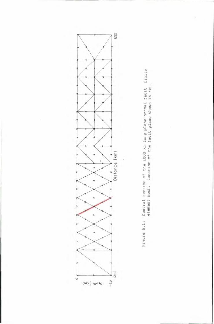
Ifl
M I c
4-J J)
3
a o O i/i C
at 0) c c m (0 . - I
a 4-1
C => o m
1 ^ u o
O t-i o o c o (0 (J o o - J c o .c u </l 0) <U in £
nj c « e c <u u <u
0)
=> CP
The mesh i s formed f r o m LOO t r i a n g u l a r i s o p a r a m e t r i c e l e m e n t s , each
h a v i n g s i x Gaussian i n t e g r a t i o n p o i n t s . The e l a s t i c p r o p e r t i e s a r e
summarised i n t a b l e 6.1. The f o l l o w i n g boundary c o n d i t i o n s were a p p l i e d :
1. The r i g h t hand edge was c o n s t r a i n e d t o move v e r t i c a l l y .
2. The l e f t hand edge was f r e e , so t h a t v a r i o u s t e n s i l e s t r e s s e s
c o u l d be a p p l i e d .
3. The base was assumed t o be u n d e r l a i n by a f l u i d w i t h a d e n s i t y o f
2900 kg m"3.
T h i s f i n i t e element mesh has i d e n t i c a l d i m e n s i o n s and p h y s i c a l p a r a m e t e r s
t o t h a t used by M i t h e n ( 1 9 8 0 ) .
PARAMETER VALUE
Young's modulus II -A Young's modulus 0.85x10 N m
Poisson's r a t i o 0.25
D e n s i t y 27 50.0 kg rrf 3
T a b l e 6.1: Values a s s i g n e d t o e l a s t i c p a r a m e t e r s o f t h e f i n i t e element model.
6.1.2 Response o f t h e f i n i t e element model t o f l e x u r e
The models o f M i t h e n (1980) p r e d i c t t h a t t h e d e f o r m a t i o n p r o d u c e d by
f r i c t i o n a l s l i d i n g on a p l a n e - s i d e d f a u l t i s d o m inated by l i t h o s p h e r i c
f l e x u r e . I t i s c o n s e q u e n t l y d e s i r a b l e t o compare t h e response o f t h e
f i n i t e element model ( s e c t i o n 6.1.1) w i t h t h e a n a l y t i c s o l u t i o n f o r t h e
f l e x u r e o f a t h i n e l a s t i c beam u n d e r l a i n by a f l u i d s u b s t r a t u m . The
a n a l y t i c s o l u t i o n t o t h i s p r o b l e m i s w e l l known ( e . g . M i t h e n , 1980).
- 101 -
So t h a t t h e a n a l y t i c and f i n i t e element s o l u t i o n s c o u l d be compared
t h e f o l l o w i n g a d d i t i o n a l boundary c o n d i t i o n s were i n i t i a l l y a p p l i e d t o t h e
model:
1. The l e f t and r i g h t hand edges o f t h e model were c o n s t r a i n e d t o
move v e r t i c a l l y .
2. The normal and shear s t i f f n e s s o f t h e f a u l t were s e t t o a h i g h
v a l u e o f 1 . 0 x l d 5 N m'so t h a t t h e ^iodel a p p r o x i m a t e s a c o n t i n u u m .
12
3. A v e r t i c a l f o r c e o f 2.0x10 MPa was a p p l i e d t o t h e c e n t r a l node (P
i n f i g u r e 6.1) o f t h e f i n i t e element mesh.
The v e r t i c a l d i s p l a c e m e n t p r o f i l e s f o r t h e two s o l u t i o n s a r e compared
i n f i g u r e 6.2. The d i s p l a c e m e n t s a r e a l m o s t i d e n t i c a l . T h i s shows t h a t
t h e f i n i t e element mesh i s c o r r e c t l y d e s i g n e d and i s s u i t a b l e f o r
p r e d i c t i n g t h e d e f o r m a t i o n a s s o c i a t e d w i t h l i t h o s p h e r i c f l e x u r e . I t a l s o 15 - i
shows t h a t t h e v a l u e o f 1.0x10 N m a s s i g n e d t o t h e n o r m a l and shear
s t i f f n e s s o f t h e f a u l t has t h e d e s i r e d e f f e c t o f making t h e model behave as
an e l a s t i c c o n t i n u u m .
T h i s t e s t was a p p l i e d t o a l l o f t h e f i n i t e element meshes o f t h i s
c h a p t e r t o check t h a t no e r r o r s had been i n t r o d u c e d i n t h e c o m p u t a t i o n a l
d e s c r i p t i o n o f t h e model and t o v e r i f y t h a t t h e mcdel was s u f f i c i e n t l y w e l l
d e f i n e d t o g i v e a c c u r a t e s o l u t i o n s t o f l e x u r a l p r o b l e m s .
6.1.3 I n i t i a l e l a s t i c d e f o r m a t i o n o f t h e model
I t was assumed i n t h e development o f t h e f a u l t model ( C h a p t e r 5) t h a t
d e f o r m a t i o n would p r o c e e d i n two phases. F i r s t l y , by an i n i t i a l e l a s t i c
d i s p l a c e p w r ^ a r i s i n g f r o m t h e c o n t r a s t i n g e l a s t i c p r o p e r t i e s o f t h e f a u l t
- 102 -
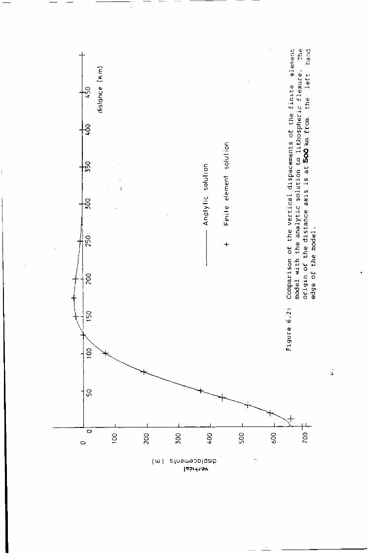
e
Qj O C _o TO
o o
o rO
O
ro
c o
o
o c <
c o
o 1/1
c I K
e 0/
c LL
o
o o
o in
o o
o in
c n c a) H m e c. 0)
0) (XI 4-1
a 0) 0) X H
4 J d) • H r H C t-J 0) r:
<M U - U • H
0) M .c o> e •*-» £ o Qi l-i
<U VI u O O « 4 J 5 C r H g a) o § 2 « U 4-> <o c m a, o l / l - H l / l H 4 J r-t T3 3
0 u
U *-> H L) 4-1
a) >, (0
01 c x: in 4-1
0) M H x: O 4-1
c JC O 4-1 Ul H
•rJ S I H rO r-t CU D §"8 u e I N
(TJ
<D U C (0
0)
0)
•8 e
o <tH
c o en a)
• H cn U TJ o a>
0) u 3 CP
o o o o (M
O O fO
O o -J
o o in o o -o
o o
(uu) S}ueuuaoD|dsip
and t h e s u r r o u n d i n g l i t h o s p h e r e , and s e c o n d l y , by f r i c t i o n a l s l i d i n g i n
o r d e r t o reduce any excess shear s t r e s s on t h e f a u l t . T h i s s e c t i o n
i l l u s t r a t e s t h e p r i m a r y s t a g e o f f a u l t d e f o r m a t i o n , t h e i n i t i a l e l a s t i c
response, and c o n t r a s t s t h e s o l u t i o n s w i t h t h o s e o f M i t h e n ( 1 9 3 0 ) .
B e f o r e i t i s p o s s i b l e t o model any f a u l t d e f o r m a t i o n , however, i t i s
n e cessary t o a s s i g n v a l u e s t o t h e normal and shear s t i f f n e s s e s o f t h e
f a u l t . These parameter;; cannot be measured a t d e p t h i n t h e e a r t h a n d
c o n s e q u e n t l y t h e v a l u e s a s s i g n e d t o them must be chosen t o c o n f o r m w i t h
o b s e r v e d f a u l t b e h a v i o u r .
The w a l l s o f t h e f a u l t would be e x p e c t e d t o be c l o s e d a t d e p t h because
of t h e l i t h o s t a t i c p r e s s u r e . The v a l u e chosen f o r t h e n o r m a l s t i f f n e s s IS - j
s h o u l d t h e r e f o r e s i m u l a t e t h i s b e h a v i o u r . The v a l u e o f 1.0x10 N m a s s i g n e d
t o t h e s t i f f n e s s o f t h e f a u l t i n t h e p r e v i o u s s e c t i o n had t h e e f f e c t o f
c l o s i n g t h e s i d e s o f t h e f a u l t and making t h e model behave as an e l a s t i c
c o n t i n u u m . The normal s t i f f n e s s o f t h e f a u l t was t h e r e f o r e a s s i g n e d a
v a l u e o f 1.0xl0 l SN m".'
Because t h e f a u l t would be e x p e c t e d t o be i n i t i a l l y l o c k e d by
a s p e r i t i e s , M i t h e n (1980) proposed t h a t t h e v a l u e o f t h e shear s t i f f n e s s o f
t h e f a u l t s h o u l d be a p p r o x i m a t e l y t h e same as t h e s t i f f n e s s o f t h e
s u r r o u n d i n g l i t h o s p h e r e . He t h e r e f o r e m o d e l l e d d e f o r m a t i o n on t h e f a u l t 10 -1
u s i n g a shear s t i f f n e s s o f 5.0x10 N m. I n c~der t o compare t h e
i s o p a r a m e t r i c model w i t h t h e CST model, the same v a l u e has been used i n
t h i s s e c t i o n . The e f f e c t o f c h a n g i n g t h e shear s t i f f n e s s i s c o n s i d e r e d
l a t e r .
F i g u r e 6.3 shows t h e v e r t i c a l d i s p l a c e m e n t and s t r e s s i n t h e c e n t r a l
s e c t i o n of t h e model when a 50 MPa t e n s i o n a l s t r e s s i s a p p l i e d t o i t s l e f t
- 103 -
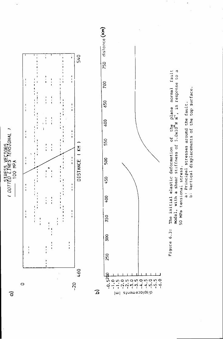
—J
1 <JT—, CUT) I—Uj
Uj Q.
m~j o ex o
o c o
T3
O Ln
o o
o un
o o
o I T i in
o o in
o in
o o • J
o m K )
O o
O in (N
Q i i i i I I 1 1 1 1 1
O
i
i n o i n o i n o m o i n o i n o o — — ojrN]hOfO-3--a-inLno
i i i i i i i i i i i i (uu) s } u e w e 3 0 | d s ) p
4-1 >—i D O m 4-J
0) 1/1
r-1 c G £ a i/i
0 m c u
c OJ c oi -a s
z (Do JC o 4->
o • O i n
4-1 c o o •r-( in
4-1 m 0) 0) e C u 4-4 o 4-1
14-1 r-4 (11 tJ
TJ l/l
U u .-1 r0 -U D
£1 ft) in rH (U ro
1—1 ffl 4-1 •H 4-1 s •H c •H
a)
<D U <0
4-1 l-( a u i
a o
01 0) £ .c 4-1 4-> T3 4 - I C O D o l-( rd
i/i
a in
c a)
in g at a) l/l (J in ro 01 i-i 4-1 (/)
X) . — I ro rH a m •H u U H C 4J H l-i u cu a, >
5 "8
U 3
ro 04 2
o in
u en
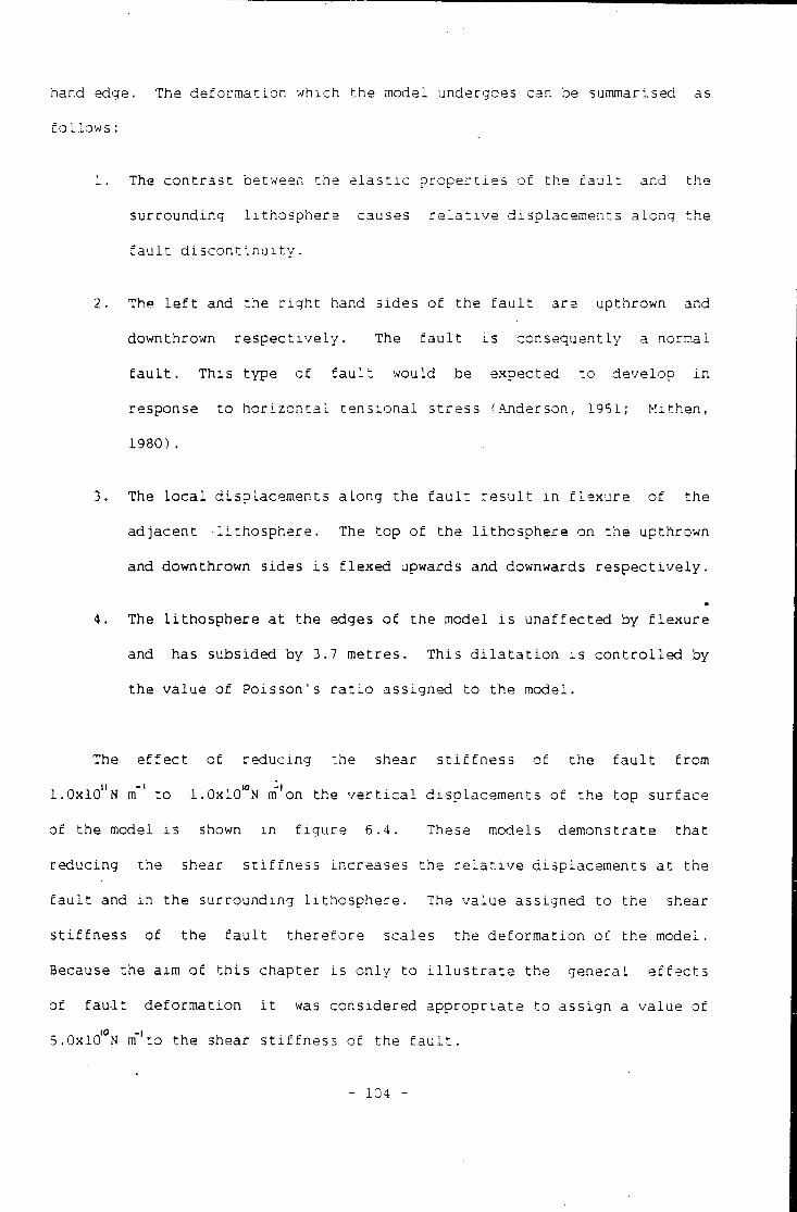
hand edge. The d e f o r m a t i o n which t h e model undergoes can be summarised as
f o l l o w s :
1. The c o n t r a s t between t h e e l a s t i c p r o p e r t i e s o f the f a u l t and t h e
s u r r o u n d i n g l i t h o s p h e r e causes r e l a t i v e d i s p l a c e m e n t s a l o n g t h e
f a u l t d i s c o n t i n u i t y .
2. The l e f t and t h e r i g h t hand s i d e s o f t h e f a u l t a r e u p t h r o w n and
downthrown r e s p e c t i v e l y . The f a u l t i s c o n s e q u e n t l y a normal
f a u l t . T h i s t y p e o f f a u l t would be e x p e c t e d t o d e v e l o p i n
response t o h o r i z o n t a l t e n s i o n a l s t r e s s (Anderson, 1951; M i t h e n ,
1980) .
3. The l o c a l d i s p l a c e m e n t s a l o n g t h e f a u l t r e s u l t i n f l e x u r e o f t h e
a d j a c e n t l i t h o s p h e r e . The t o p o f t h e l i t h o s p h e r e on t h e u p t h r o w n
and downthrown s i d e s i s f l e x e d upwards and downwards r e s p e c t i v e l y .
4. The l i t h o s p h e r e a t t h e edges o f t h e model i s u n a f f e c t e d by f l e x u r e
and has s u b s i d e d by 3.7 m e t r e s . T h i s d i l a t a t i o n i s c o n t r o l l e d by
t h e v a l u e o f Poisson's r a t i o a s s i g n e d t o t h e model.
The e f f e c t o f r e d u c i n g the shear s t i f f n e s s o f t h e f a u l t f r o m
1.0X10"N m ' t o 1 . 0 x 1 0 % nf'on t h e v e r t i c a l d i s p l a c e m e n t s o f t h e t o p s u r f a c e
o f t h e model i s shown i n f i g u r e 6.4. These models d e m o n s t r a t e t h a t
r e d u c i n g t h e shear s t i f f n e s s i n c r e a s e s t h e r e l a t i v e d i s p l a c e m e n t s a t t h e
f a u l t and i n t h e s u r r o u n d i n g l i t h o s p h e r e . The v a l u e a s s i g n e d t o t h e shear
s t i f f n e s s o f t h e f a u l t t h e r e f o r e s c a l e s t h e d e f o r m a t i o n o f t h e . m o d e l .
Because t h e aim o f t h i s c h a p t e r i s o n l y t o i l l u s t r a t e t h e g e n e r a l e f f e c t s
o f f a u l t d e f o r m a t i o n i t was c o n s i d e r e d a p p r o p r i a t e t o a s s i g n a v a l u e o f
5.0xl0'°N nf'to t h e shear s t i f f n e s s o f t h e f a u l t .
- 104 -
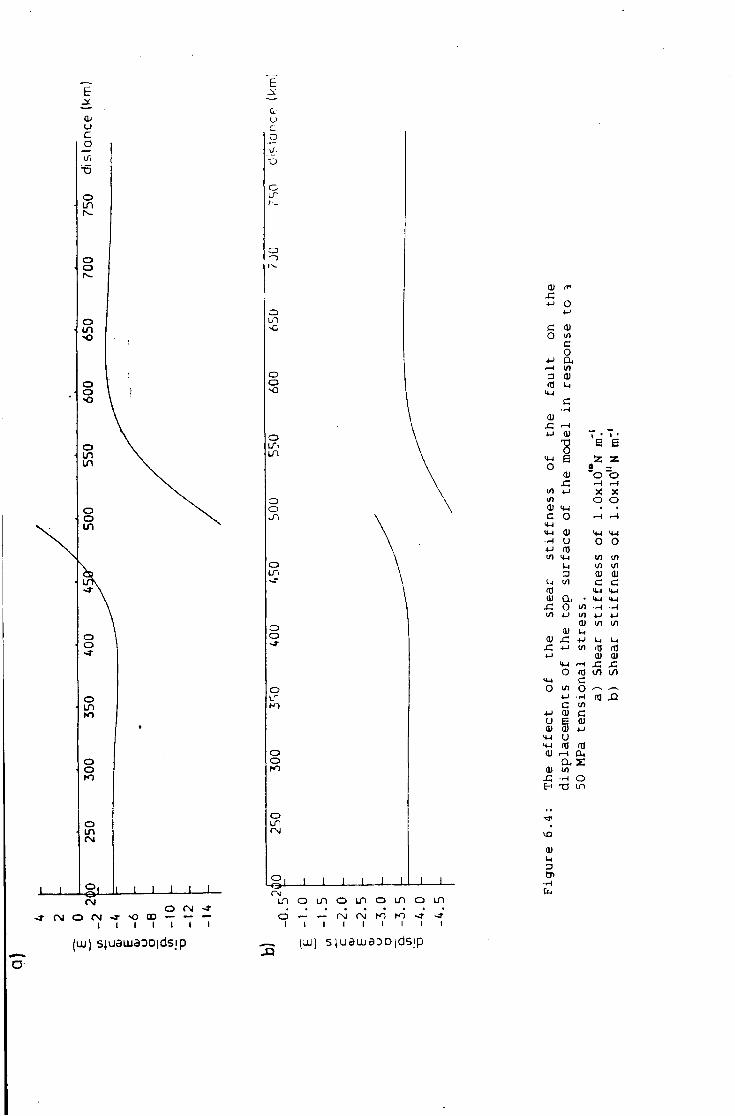
' — 0 Qj U U r~ c o o u. l/l X) T5
o LP in r -f -
o o — i o i ^ -
o o in i n S3 !
I o o 1 o O \ 1 SD •o \
\ o o \ LTi i n \ in i n \
o o \. o O \ j~< \ i n
\ v o
in
\ o o o o ~r
o o i n H I
• O
o o o K )
O O in i n r>j rsi
o. 1 1 o.
— L I 1 1 1-1 J I L J L
O <N «* ^ M O f M - f - O O D - - -
I I I I I I I
(UJ) sjuawaDD|dsjp
m o m o i n o i n o m o
i — — fM (M K ) ro
I I I I I I I
01 c x : 4-1 O
J-J
c 0) o in
c o
4-1 a, in 3 01
IB 1-1 M-l
c
0) XI i—1 4 J 0) i • "8 S E
M-l E 55 z o a —
01 " o " b x : r - l r-4
1/1 *-> X 1/1 o o 0) M-l • «
c o ,-1 <4-l <*-! •H u o 0 4 J rO in M-l m in U in in
=J 01 01 in C C
<0 M-l MJ 01 a • M-4 M-4
x : o in •H in in 4-1 +-> Oi m in
01 i-i 0) x : u i-i i j n 4-J in fO rO u 0> 01
M-l H x ; x : o m to u-l c
O in o ^ •H rO C in •u Q) C u 0) 0> 01 4-1
M-l u MJ ra <D r-t a.
a x 0> m x : •H o
in
l£>
01 Ul D en •H
^ (UU) 5 J U d U U a D D j d S j P
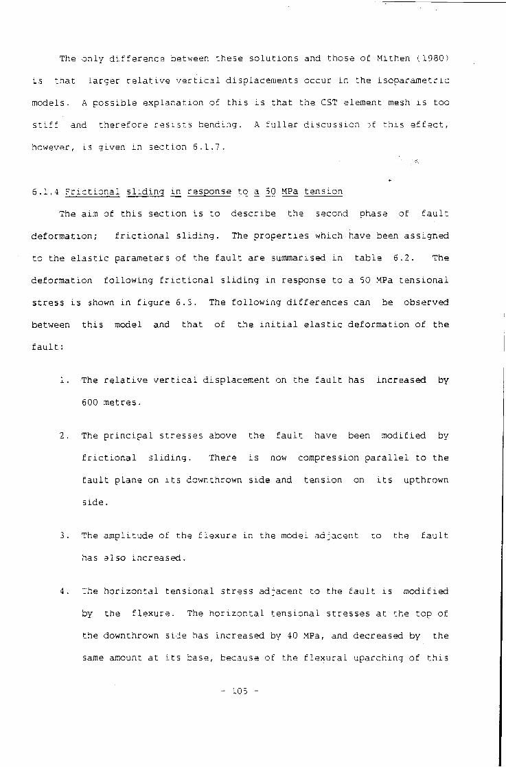
The o n l y d i f f e r e n c e between t h e s e s o l u t i o n s and t h o s e o f M i t h e n (1980)
i s t h a t l a r g e r r e l a t i v e v e r t i c a l d i s p l a c e m e n t s o c c u r i n t h e i s o p a r a m e t r i c
models. A p o s s i b l e e x p l a n a t i o n o f t h i s i s t h a t t h e CST element mesh i s t o o
s t i f f and t h e r e f o r e r e s i s t s b e n d i n g . A f u l l e r d i s c u s s i o n of t h i s e f f e c t ,
however, i s g i v e n i n s e c t i o n 6.1.7.
6.1.4 F r i c t i o n a l s l i d i n g i n response t o a 50 MPa t e n s i o n
The aim o f t h i s s e c t i o n i s t o d e s c r i b e t h e second phase o f f a u l t
d e f o r m a t i o n ; f r i c t i o n a l s l i d i n g . The p r o p e r t i e s w h i c h have been a s s i g n e d
t o t h e e l a s t i c p a rameters o f t h e f a u l t a r e summarised i n t a b l e 6.2. The
d e f o r m a t i o n f o l l o w i n g f r i c t i o n a l s l i d i n g i n response t o a 50 MPa t e n s i o n a l
s t r e s s i s shown i n f i g u r e 6.5. The f o l l o w i n g d i f f e r e n c e s can be o b s e r v e d
between t h i s model and t h a t o f t h e i n i t i a l e l a s t i c d e f o r m a t i o n o f t h e
f a u l t :
1. The r e l a t i v e v e r t i c a l d i s p l a c e m e n t on t h e f a u l t has i n c r e a s e d by
600 m e t r e s .
2. The p r i n c i p a l s t r e s s e s above t h e f a u l t have been m o d i f i e d by
f r i c t i o n a l s l i d i n g . There i s now c o m p r e s s i o n p a r a l l e l t o t h e
f a u l t p l a n e on i t s downthrown s i d e and t e n s i o n on i t s u p t h r o w n
s i d e .
3. The a m p l i t u d e o f t h e f l e x u r e i n t h e model a d j a c e n t t o t h e f a u l t
has a l s o . i n c r e a s e d .
4. The h o r i z o n t a l t e n s i o n a l s t r e s s a d j a c e n t t o t h e f a u l t i s m o d i f i e d
by t h e f l e x u r e . The h o r i z o n t a l t e n s i o n a l s t r e s s e s a t the t o p o f
t h e downthrown s i d e has i n c r e a s e d by 40 MPa, and d e c r e a s e d by t h e
same amount a t i t s base, because o f t h e f l e x u r a l u p a r c h i n g o f t h i s
- 105 -
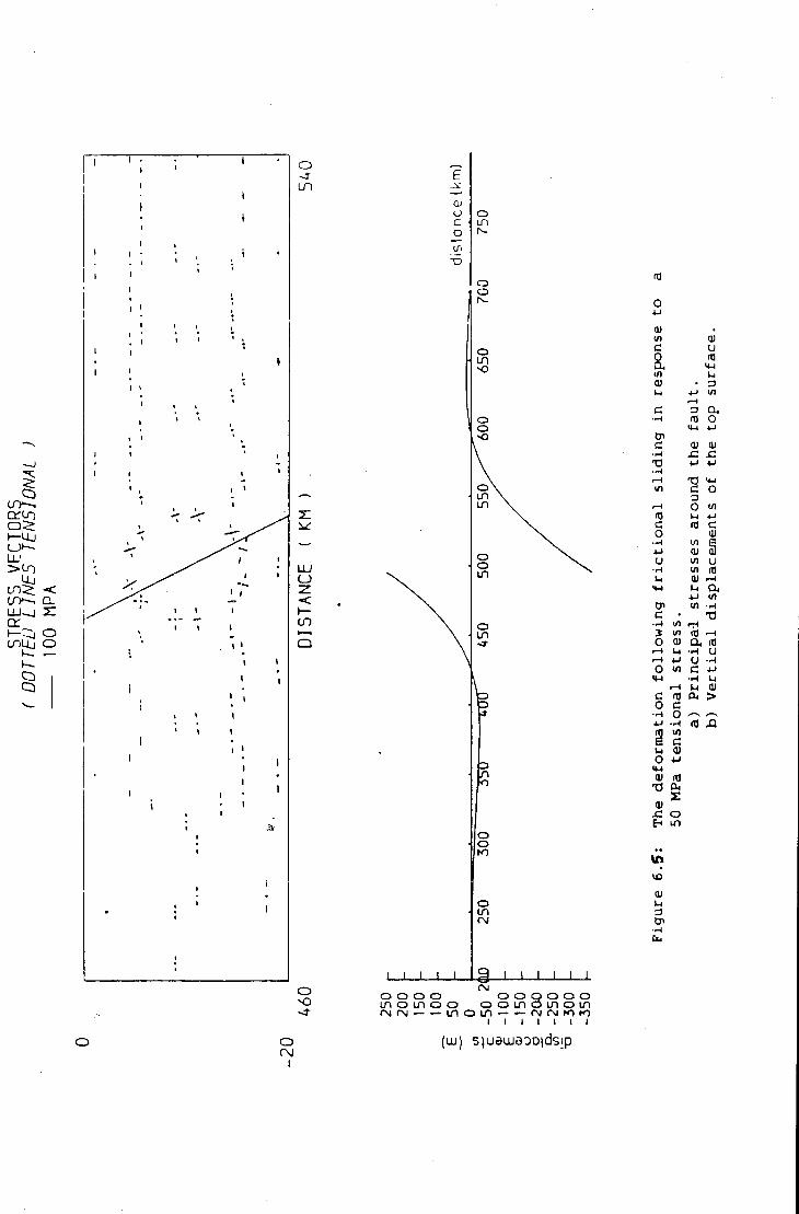
— —J
or co a 5 <_»— 1 1 I LL.
t n ^ . •< CO*-, CL UJ^J J :
or i — o cnuj o
. —
—
< I I >
o - J -
o
E
cu o c o T3
O
o o
o i n
I I I I
o i n
n
o o
o i n CM
I I I I I I o o o o i n o i n o o CNJ r \ j — — m
rsi o o o o o o
o o i n o in o in o i n — — I N rg K i m
i i i i i i i
O i
(UJI sjuaoieoDidsip
0 4J 0) l/l a) c u 0 (0 a, in i j • l-l 4J i/i
r—1 c a •H rU o
M-l 4-1 c 1) 0)
•H x: x: T3 4-1 *-> —4 r - l T3 l*-l 1/1 C o f—4 0 Ul (TJ 4J C c 0 a)
VI 4-1 <u <D u l/l u •-4 1/1 in u 01
i-l a, 4-1 i/i l/l
C • •o —4 rrl 3 i/i 0 ai a,
u • H u 4-1 u •H
o i/i c 4-1 <t-J • H 14
I-l 01 c (0 a. > o c •-4. 0 4J
1/) g e u ai o 4-> <D T3 T3 0) .c o H m
I-l 3 en - 4
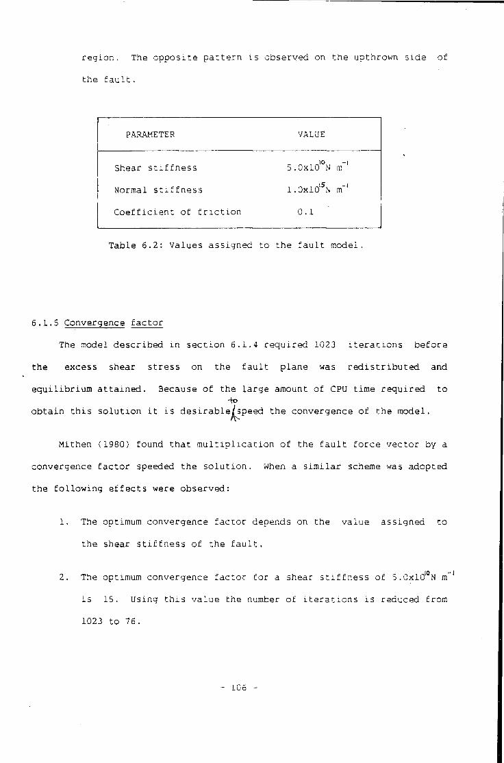
r e g i o n . The o p p o s i t e p a t t e r n i s o b s e r v e d on t h e u p t h r o w n s i d e o f
t h e f a u l t .
PARAMETER VALUE
Shear s t i f f n e s s 5.0x10 N m - i
Normal s t i f f n e s s 1.0xlo' 5N m' - i
C o e f f i c i e n t o f f r i c t i o n 0.1
T a b l e 6.2: Values a s s i g n e d t o t h e f a u l t model.
6.1.5 Convergence f a c t o r
The model d e s c r i b e d i n s e c t i o n 6.1.4 r e q u i r e d 1023 i t e r a t i o n s b e f o r e
t h e excess shear s t r e s s on t h e f a u l t p l a n e was r e d i s t r i b u t e d and
e q u i l i b r i u m a t t a i n e d . Because o f t h e l a r g e amount o f CPU t i m e r e q u i r e d t o
o b t a i n t h i s s o l u t i o n i t i s d e s i r a b l e / s p e e d t h e convergence o f t h e model.
M i t h e n (1980) f o u n d t h a t m u l t i p l i c a t i o n o f t h e f a u l t f o r c e v e c t o r by a
convergence f a c t o r speeded t h e s o l u t i o n , when a s i m i l a r scheme was a d o p t e d
t h e f o l l o w i n g e f f e c t s were o b s e r v e d :
1. The optimum convergence f a c t o r depends on t h e v a l u e a s s i g n e d t o
t h e shear s t i f f n e s s o f t h e f a u l t .
2. The optimum convergence f a c t o r f o r a shear s t i f f n e s s o f 5.0xl0 l oN m
i s 15. Using t h i s v a l u e t h e number o f i t e r a t i o n s i s reduced from
1023 t o 76.
- 106 -
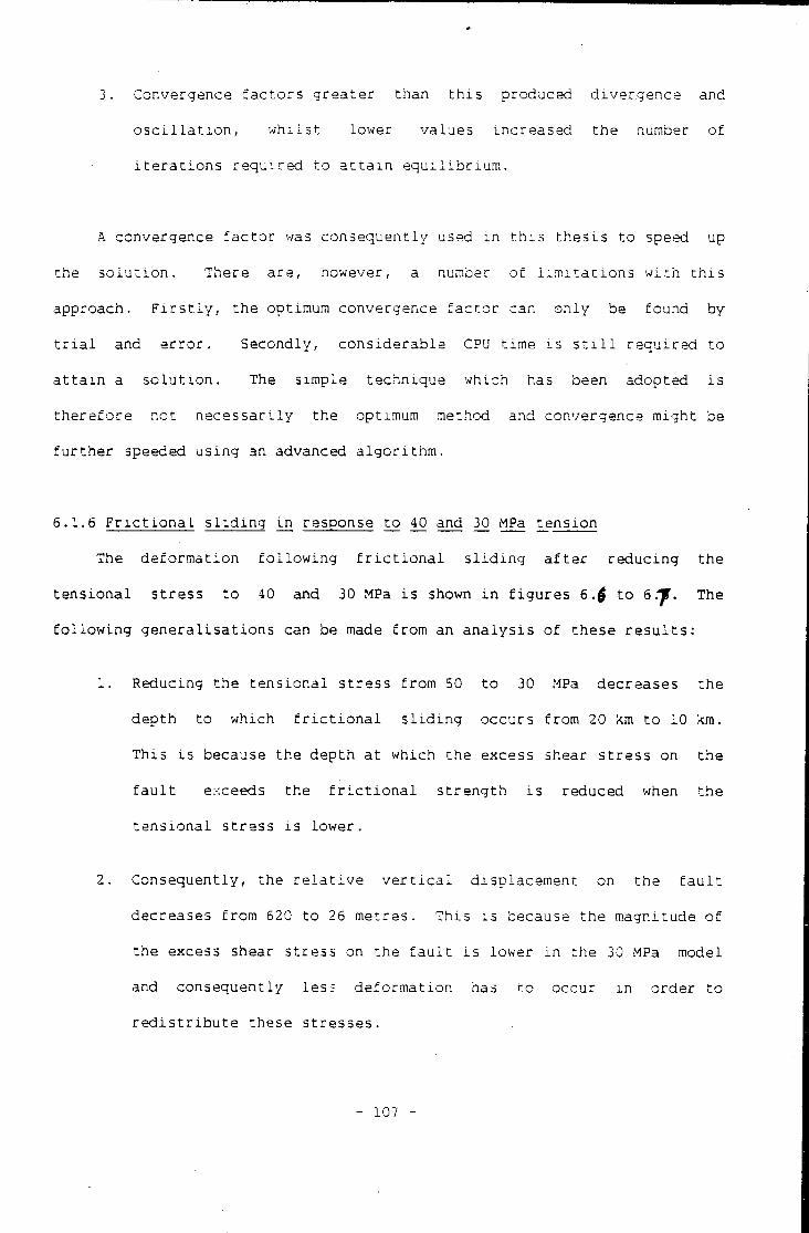
3. Convergence f a c t o r s g r e a t e r t h a n t h i s produced d i v e r g e n c e and
o s c i l l a t i o n , w h i l s t lower v a l u e s i n c r e a s e d t h e number o f
i t e r a t i o n s r e q u i r e d t o a t t a i n e q u i l i b r i u m .
A convergence f a c t o r was c o n s e q u e n t l y used i n t h i s t h e s i s t o speed up
t h e s o l u t i o n . There a r e , however, a number o f l i m i t a t i o n s w i t h t h i s
approach. F i r s t l y , t h e optimum convergence f a c t o r can o n l y be f o u n d by
t r i a l and e r r o r . Secondly, c o n s i d e r a b l e CPU t i m e i s s t i l l r e q u i r e d t o
a t t a i n a s o l u t i o n . The s i m p l e t e c h n i q u e w h i c h has been a d o p t e d i s
t h e r e f o r e n o t n e c e s s a r i l y t h e optimum method and convergence m i g h t be
f u r t h e r speeded u s i n g an advanced a l g o r i t h m .
6.1.6 F r i c t i o n a l s l i d i n g i n response t o 40 and 30 MPa t e n s i o n
The d e f o r m a t i o n f o l l o w i n g f r i c t i o n a l s l i d i n g a f t e r r e d u c i n g t h e
t e n s i o n a l s t r e s s t o 40 and 30 MPa i s shown i n f i g u r e s 6.$ t o 6/^. The
f o l l o w i n g g e n e r a l i s a t i o n s can be made f r o m an a n a l y s i s o f t h e s e r e s u l t s :
1. Reducing t h e t e n s i o n a l s t r e s s f r o m 50 t o 30 MPa d e c r e a s e s t h e
d e p t h t o w h i c h f r i c t i o n a l s l i d i n g o c c u r s from 20 km t o 10 km.
T h i s i s because t h e d e p t h a t w h i c h t h e excess shear s t r e s s on t h e
f a u l t exceeds t h e f r i c t i o n a l s t r e n g t h i s reduced when t h e
t e n s i o n a l s t r e s s i s l o w e r .
2. C o n s e q u e n t l y , t h e r e l a t i v e v e r t i c a l d i s p l a c e m e n t on t h e f a u l t
d e creases f r o m 620 t o 26 m e t r e s . T h i s i s because t h e magnitude o f
t h e excess shear s t r e s s on t h e f a u l t i s lower i n t h e 30 MPa model
and c o n s e q u e n t l y l e s s d e f o r m a t i o n has t o o c c u r i n o r d e r t o
r e d i s t r i b u t e t h e s e s t r e s s e s .
- 107 -
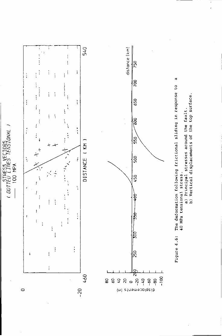
o un
E
QJ O c o
T5
o in
o o
o in -o
o O
f
0) l / l 01 c u
m in u o> • U 4-J l / l
1—1 C 3 a
(0 o VI •u CP
c 01 •H x: T> 4J 4-1 •H 1-4, X) 4-4 l / l c o r-t o l / l TJ u 4 J C ITJ c 0 01
•-4 Ul 6 4J 01 a) u l / l u
•H ui m l j 0) i-H U-l u a,
4-1 V I <7> l / l
C • •a •H 1—1
in (0 i - i 0 01 Q, it) r-4 u •H u r~i 4-1 U ••H 0 in c 4-1
"4-1 •r-1 1-4 rH U 0)
c (X > o c •H 0 —* 4 J •f-l
l / l £ c l-i 01 0 4->
<u (0 T3
0) JC o Til
lO
01 u 3 tn •H Li
o o o o o o o o o O D O » I - < M O ( M > * > O C D —
O CM
I
(w) s |ueajaoD|ds ip
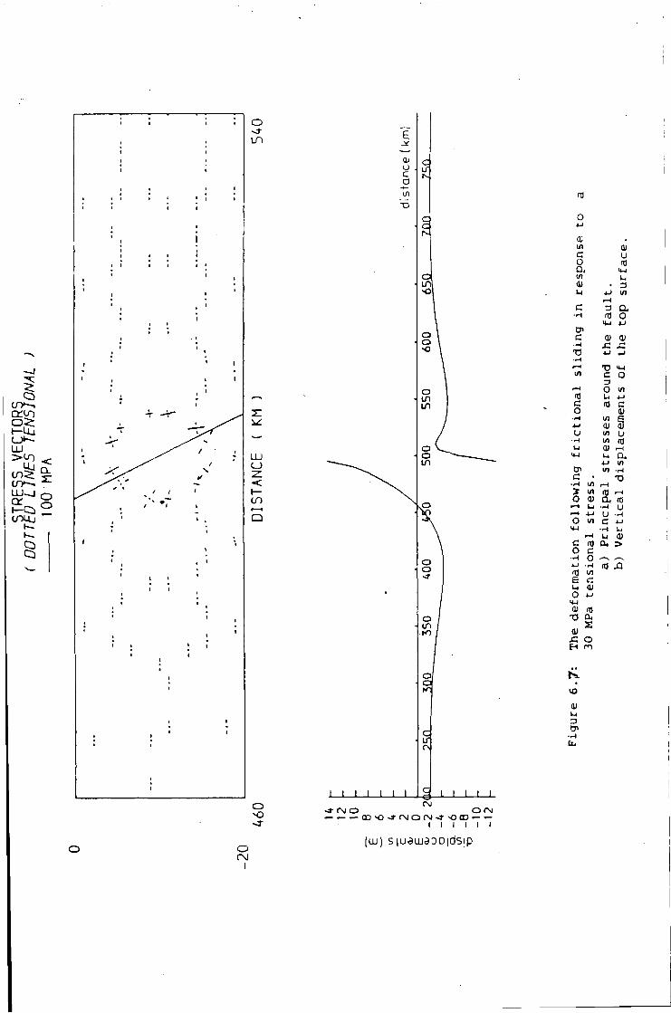
o - J -LTl E
l_l c a
T3
I I I I I I I
c IT
C c N
I I I I 1 o - J -
o i
- j - rsi o o r\j - - — 0 D O J T \ l o r M J - - O C D - -
I I I I I I
(uu) S ) u e w a o D | d s i p
o 4 J
a in c u o ro a, 4-1 Ul Li 0) • D U 4-> in
i-H c 3 a,
• H rfl 0 •4-4 4-1
Cn C 01
• H SZ sz T ) 4-J 4-1 • H .-1 T) 4-1 1/) C o
i-H O in T3 u 4-1 C rfl c o CD
in 4 J aj 5J U m u
•H m ro Ll <U i—i
M-l u a. 4-1 in
C7> in C • T3
• H l/l r-1 J «/l ra r-l o <u a. rO r-l U —i U r-t 4-1 u •~l O m c 4 J •W • H Li
•-4 Li C <T3 04 > o c -4 o .—. 4-J H rO ra w s c O 4 J
4-1 ai m -o o.
a> £ o
ai Li a cn [14
3. The a m p l i t u d e o f t h e f l e x u r e i n t h e model a d j a c e n t t o t h e f a u l t i s
reduced. T h i s d e c r e a s e s t h e magnitude o f t h e h o r i z o n t a l t e n s i o n a l
s t r e s s a t t h e t o p o f t h e model on t h e downthrown s i d e o f t h e
f a u l t .
4. At low t e n s i o n a l s t r e s s e s a s h o r t w a v e l e n g t h upwards f l e x u r e
occurs, on t h e downchrown Side o f t h e f a u l t . T h i s f l e x u r e , w h i c h
has i t s a x i s a t 15 km from d i e f a u l t p l a n e , has p r e v i o u s l y been
n o t e d by M i t h e n ( 1980)". T h i s f l e x u r e c ; c u r s when f r i c t i o n a l
s l i d i n g has n o t p e n e t r a t e d t h r o u g h o u t t h e e l a s t i c l a y e r and i t i s
th e r e s u l t o f f l e x u r e above a c o n t i n u o u s e l a s t i c s u b s t r a t u m .
These r e s u l t s a r e q u a l i t a t i v e l y s i m i l a r t o t h o s e o b t a i n e d by M i t h e n
(1980) who p e r f o r m e d i d e n t i c a l t e s t s w i t h CST e l e m e n t s . The major
d i f f e r e n c e i s t h a t t h e r e l a t i v e d i s p l a c e m e n t s o f t h e i s o p a r a m e t r i c model
a r e c o n s i s t e n t l y h i g h e r t h a n t h a n t h o s e o f t h e CST model: f o r 50 MPa t h e
th r o w o f t h e f a u l t i n t h e i s o p a r a m e t r i c models i s 100 metres g r e a t e r .
L a r g e r t e n s i o n s c o n s e q u e n t l y o c c u r a t t h e t o p o f t h e downthrown s i d e o f t h e
f a u l t i n t h e i s o p a r a m e t r i c model. The i m p l i c a t i o n s and o r i g i n s o f t h e s e
d i f f e r e n c e s a r e d i s c u s s e d i n t h e n e x t s e c t i o n .
6.1.7 P r e d i c t e d graben w i d t h s
The models p r e s e n t e d i n s e c t i o n 6.1.6 d e m o n s t r a t e t h a t l a r g e near
s u r f a c e h o r i z o n t a l t e n s i o n a i s t r e s s o c c u r s on t h e downthrown s i d e o f t h e
f a u l t because o f t h e f l e x u r e produced by f r i c t i o n a l s l i d i n g . A consequence
o f t h i s i s t h a t t e n s i o n a i f a i l u r e i s l i k e l y t o o c c u r on t h e downthrown s i d e
o f t h e f a u l t . The m o d i f i e d G r i f f i t h t h e o r y i s t h e r e f o r e used i n t h i s
s e c t i o n t o p r e d i c t t h e d i s t a n c e from t h e f a u l t where f a i l u r e i s most l i k e l y
t o o c c u r . T h i s d i s t a n c e w i l l be r e f e r r e d t o as t h e p r e d i c t e d graben w i d t h .
- 103 -
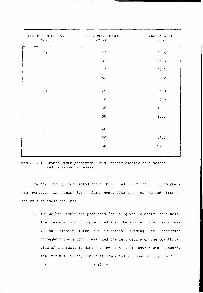
ELASTIC THICKNESS (km)
TENSIONAL STRESS (MPa)
GRABEN WIDTH (km)
10 20 22 .5
30 26 . 5
40 0-7 i
50 27.2
20 20 15.0
40 15.0
60 45 .5
80 45.5
30 40 10.5
60 17 .0
80 57 .5
T a b l e 6.3: Graben w i d t h p r e d i c t e d f o r d i f f e r e n t e l a s t i c t h i c k n e s s e s and t e n s i o n a l s t r e s s e s .
The p r e d i c t e d graben w i d t h s f o r a 10, 20 and 30 km t h i c k l i t h o s p h e r e
a r e compared i n t a b l e 6.3. Some g e n e r a l i s a t i o n s can be made f r o m an
a n a l y s i s o f t h e s e r e s u l t s :
1. Two graben w i d t h s a r e p r e d i c t e d f o r a g i v e n e l a s t i c t h i c k n e s s .
The maximum w i d t h i s p r e d i c t e d when t h e a p p l i e d t a n s i o n a l s t r e s s
i s s u f f i c i e n t l y l a r g e f o r f r i c t i o n a l s l i d i n g t o p e n e t r a t e
t h r o u g h o u t t h e e l a s t i c l a y e r and t h e d e f o r m a t i o n on t h e downthrown
s i d e o f t h e f a u l t i s d o m inated by t h e l o n g w a v e l e n g t h f l e x u r e .
The minimum w i d t h , which i s p r e d i c t e d a t lower a p p l i e d t e n s i o n ,
- 109 -
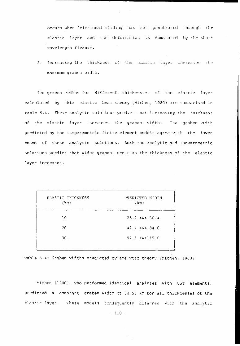
o c c u r s when f r i c t i o n a l s l i d i n g has n o t p e n e t r a t e d t h r o u g h t h e
e l a s t i c l a y e r and t h e d e f o r m a t i o n i s d o m i n a t e d by t h e s h o r t
w a v e l e n g t h f l e x u r e .
2. I n c r e a s i n g t h e t h i c k n e s s o f t h e e l a s t i c l a y e r i n c r e a s e s t h e
maximum graben w i d t h .
The graben w i d t h s f o r d i f f e r e n t t h i c k n e s s e s o f t h e e l a s t i c l a y e r
c a l c u l a t e d by t h i n e l a s t i c beam t h e o r y ( M i t h e n , 1980) a r e summarised i n
t a b l e 6.4. These a n a l y t i c s o l u t i o n s p r e d i c t t h a t i n c r e a s i n g t h e t h i c k n e s s
o f t h e e l a s t i c l a y e r i n c r e a s e s t h e graben w i d t h . The graben w i d t h
p r e d i c t e d by t h e i s o p a r a m e t r i c f i n i t e element models agree w i t h t h e lower
bound o f these a n a l y t i c s o l u t i o n s . Both t h e a n a l y t i c and i s o p a r a m e t r i c
s o l u t i o n s p r e d i c t t h a t w i d e r grabens occur as t h e t h i c k n e s s o f t h e e l a s t i c
l a y e r i n c r e a s e s .
ELASTIC THICKNESS PREDICTED WIDTH (km) (km)
10 25.2 <w< 50.4
20 42.4 <w< 84.0
30 57.5 <w<115.0
Tabl e 6.4: Graben w i d t h s p r e d i c t e d by a n a l y t i c t h e o r y ( M i t h e n , 1980)
M i t h e n ( 1 9 8 0 ) , who p e r f o r m e d i d e n t i c a l a n a l y s e s w i t h CST el e m e n t s ,
p r e d i c t e d a c o n s t a n t graben w i d t h of 50-55 km f o r a l l t h i c k n e s s e s o f t h e
e l a s t i c l a y e r . • These models r o n s e q u e n t l y d i s a g r e e w i t h t h e a n a l y t i c
- 110 -
s o l u t i o n s . M i t h e n (1980) proposed t h a t t h i s d i s c r e p a n c y a r o s e because t h e
a p p r o x i m a t i o n s made i n t h e t h i n e l a s t i c beam s o l u t i o n s o v e r s i m p l i f y t h e
t r u e c o m p l e x i t y o f t h e p r o b l e m .
The agreement between t h e graban w i d t h s p r e d i c t e d by t h e a n a l y t i c
s o l u t i o n s and t h e i s o p a r a m e t r i c models o f t h i s t h e s i s , however, suggests an
a l t e r n a t i v e e x p l a n a t i o n ; t h e CST meshes w h i c h were used by Mi t h e n (1980)
a r e t o o s t i f f t o a c c u r a t e / model l i t h o s p h a r i c f l e x u r e . T h i s c o n c l u s i o n i s
s u p p o r t e d by t h e o b s e r v a t i o n s i n p r e v i o u s s e c t i o n s o f t h i s c h a p t e r t h a t t h e
d i s p l a c e m e n t s o f t h e CST models a r e c o n s i s t e n t l y l e s s t h a n t h o s e o f t h e
i s o p a r a m e t r i c s o l u t i o n s . As shown i n Chapter 4 t h i s commonly o c c u r s i n
f l e x u r a l problems when t h e CST f i n i t e element mesh i s t o o s t i f f because an
i n s u f f i c i e n t number o f elements have been used t o model t h e l i n e a r s t r a i n
g r a d i e n t . M i t h e n ( 1 9 8 0 ) , however, used r e l a t i v e l y c o a r s e CST e l e r r ^ n t
meshes t o e x t e n d h i s a n a l y s i s t o p r e d i c t graben w i d t h s i n much more complex
s i t u a t i o n s . Those o f M i t h e n ' s c o n c l u s i o n s w h i c h a r e dependent upon t h e
f l e x u r a l response o f CST meshes s h o u l d tto.re.fore. be t r e a t e d c a u t i o u s l y u n t i l
v e r i f i e d by i s o p a r a m e t r i c s o l u t i o n s .
6.1.8 I s o s t a t i c c o mpensation on t h e upper s u r f a c e o f t h e model
Some o f t h e models i n t h e p r e v i o u s s e c t i o n s show l a r g e v e r t i c a l
d i s p l a c e m e n t s o f t h e t o p s u r f a c e o f t h e model. I n r e a l i t y i s o s t a t i c
r e s t o r i n g f o r c e s oppose t h e development o f l a r g e v e r t i c a l upward o r
downward d i s p l a c e m e n t s . An i s o s t a t i c r e s t o r i n g f o r c e e q u i v a l e n t t o t h e
t o p o g r a p h i c l o a d on t h e t o p s u r f a c e o f t h e model i s t h e r e f o r e i n t r o d u c e d i n
t h i s s e c t i o n . T h i s compensation p r o c e d u r e i s i d e n t i c a l t o t h a t a p p l i e d a t
t h e base o f t h e f i n i t e element models.
- I l l -
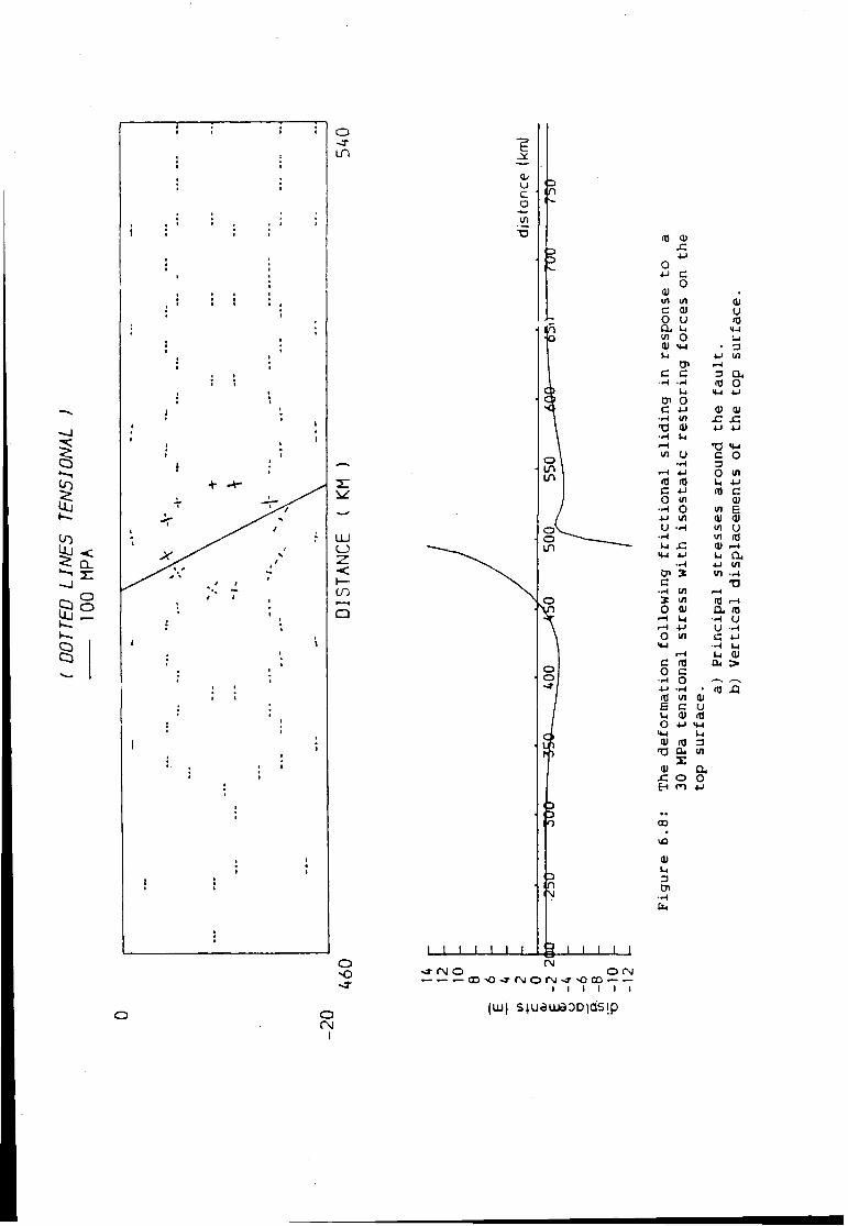
1
to £ Q.
§ 2
C5
o -3" I f )
E -X dl l_> c o in
o n
3
I I I I I I 1
O O I 0
o (M •J- rvj o o rsj — • < r > o - j - r \ i o r \ i < r - o c o ^ ^
i i i i i i
O
i (LU) s j u e u B O D i d s i p
01
the
o 4-1
on
0) • l / l in 01 c 01 u o U m cu u I J l / l 0 '—1
M-l • 3 u
01 *-> in
c c 3 a u fa
to
cn O c 4-> o> 01
-H" l / l x: x: T ) <U 4-J 4-1 •H I-l i - l •a <M
l / l u •H
un O i - l 4-1 0 in
IT) H) Ul 4-1 c 4-1 I D C 0 in 01
•H o in p 4-1 71 01 ol u •H in u
•-I in fO U x: 0) r—1
V I 4 J u a. •H 4-1 in
CP in •f-i c •a •w in i—i % in a) r-4 0 at a, m
i-i • H u r-H • M u • H
fo
in c ••4
4-1 Ll
r H u 0) c m cu > o c
•.-4 o —V 4-> • H • a) XI IT) l / l 01 a c u l-l 0) m
fo
4-1
rf
m 3 T3 0 4 Ul T3
m a, J C o o H en *->
00
lO
01 Ul 3 0 i
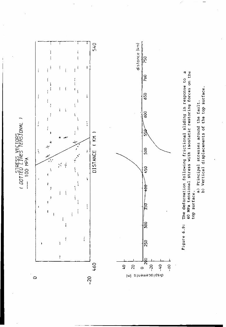
uy—i
t-Uj <_)•-. U J
t—Q
£ QJ O c o to
o
the
o 4-1
on
QJ • 1/1 </i 0) C 0) u o u m a , u <4-l i/i o L l
• 3 L i
O i It
i/l
c c 3 a •r4. •-4,
u fa
to
0 c 4 J 01 ai
•r-t l/l xz T3 01 4-1 4-1 • H L i r- l <t-l i/l
ic
un o
*—* 4-1 0 l/l Hi L i 4 J
c 4-1 nj c o l/l 0>
0 in 4-1 l/l 01 oi u • H i/i u
• H >/> nj u JC 0) •—1
<*J 4-> L , a •r4 4 J l/l
cn X VI • H c n
• H l/l r-4 s 1/1 ns »—i 0 0) a , m
L i u 4-1 u • H
fo
i/l
in 4-1
L i r-l L i 0)
c 04 > o c • H o —^ 4-1 XI ITJ l/l e c u L i 01 HJ o *J >M
<«-l L i no 3
T3 04 V) T3 X
oi a , o o
H 4 J
OS
a> Li a Cn
O (NJ I
(UJ) s )uau j30D|ds ip
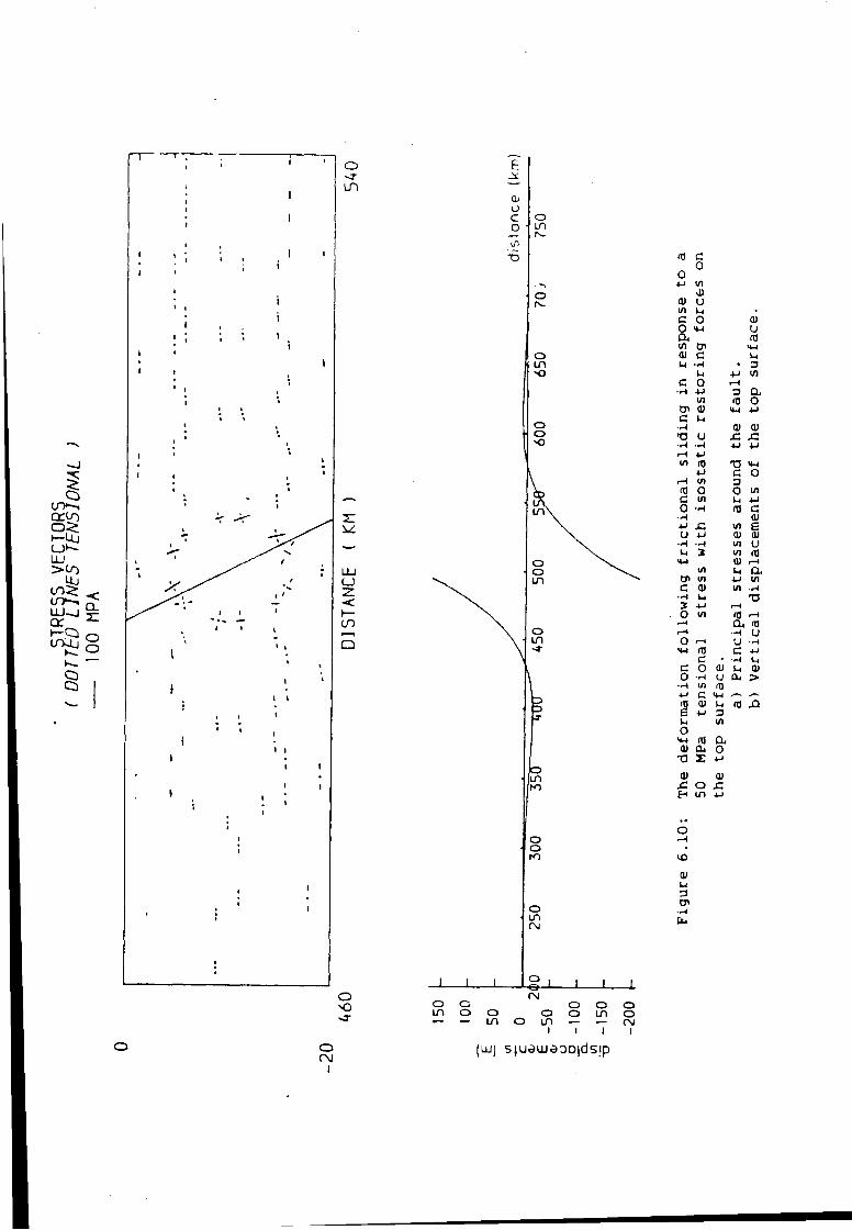
- J
1 H - U j (_)•--U J
IT*-, 5 cr i-c n i u g
< I
O
LTl
E
O c o o LTl
ID TO
O
o i n -o
o o
i n \
O o \ -m
o \ • i n
<r
\ \
ID
J -
O i n
o o r o
o i n r\i
i i i ° i i i i —i i ' J 1 1 L o o
o CM I
o o o o o i n o o o o i n o •— — i n o u n — =— CM
i i i i
(UJ) s juaweoDids ip
(TJ c 0
o u W
d) 0) u in u • c o 0) o •4-1 u a . in V-4 01 c u
•H • D •M l/l
C 0 r-t •*-t 4-> 3 a ,
1/1 HJ o Q) •4-4 4-1
c l-i <D 0)
T3 U JZ • H 4-1 4-J
r-( 4-J 10 73 >4-4 4-1 C o
c- l Ul a m O o in c VI 4-1 0 •H (0 c
—1 <D 4 J x ; 1/1 e u 4-1 ai 0)
• H • H in u Ul in
<4-l <U Ul L i a
cn in 4-1 in c a) in • r-l
u * 4-1 r-4 o i/i (0 r-H
.-H a <—1 • H u 0 i—i u
ra c 4-J c • Ul
c o at 0) 0 •H u a , > 1/1 m
4 J c <u -— ng 0) U m
4-1 D Ui 1/1 O
"4-1 m a 0) o
• a s 4 J
dJ
£. o H i n 4-1
a>
The e f f e c t o f i n t r o d u c i n g t h i s boundary c o n d i t i o n t o t h e models w h i c h
have 30, 40 and 50 MPa t e n s i o n a p p l i e d t o them i s shown i n f i g u r e s 6.8 t o
6.10. Comparing t h e s e r e s u l t s w i t h t h e p r e v i o u s s o l u t i o n s ( s e c t i o n 6.1.5)
de m o n s t r a t e s t h a t t h e i n t r o d u c t i o n o f t h e i s o s t a t i c r e s t o r i n g f o r c e s on t h e
to p s u r f a c e reduces t h e l a r g e v e r t i c a l d i s p l a c e m e n t s i n t h e 50 and 40 MPa
models, b u t has l i t t l e e f f e c t on t h e s m a l l e r d i s p l a c e m e n t s i n t h e 30 MPa
s o l u t i o n . The o v e r a l l shape o f t h e d i s p l a c e m e n t p r o f i l e i n t h e s u r r o u n d i n g
l i t h o s p h e r e , however, i s unchanged. C o n s e q u e n t l y , t h e p r e d i c t e d g r a b e n
w i d t h s do n o t d i f f e r f r o m t h e p r e v i o u s s o l u t i o n .
Because t h i s boundary c o n d i t i o n i s c o n s i d e r e d t o be r e a l i s t i c i t i s
a p p l i e d t o t h e models which a r e p r e s e n t e d i n l a t e r s e c t i o n s o f t h i s
c h a p t e r .
6.2 L i s t r i c Normal F a u l t
• The r e s u l t s o f s e c t i o n 6.1 d e m o n s t r a t e t h a t t h e model o f f r i c t i o n a l
s l i d i n g a c c u r a t e l y s i m u l a t e s t h e d e f o r m a t i o n on a p l a n e normal f a u l t . T h i s
a n a l y s i s i s now e x t e n d e d t o p r e d i c t t h e d e f o r m a t i o n on l i s t r i c n o r m a l
f a u l t s . T h i s s e c t i o n compares and c o n t r a s t s t h e m o d e l l e d d e f o r m a t i o n on a
l i s t r i c n o rmal f a u l t w i t h t h a t on p l a n e normal f a u l t s .
6.2.1 D e s c r i p t i o n o f t h e f i n i t e element mesh
The c e n t r a l s e c t i o n o f t h e 800 '<m l o n g f i n i t e element mesh and t h e
p o s i t i o n o f t h e l i s t r i c f a u l t a r e shown i n f i g u r e 6.11. The f a u l t has t h e
f o l l o w i n g geometry:
1. Between t h e s u r f a c e and 10 km i t i s p l a n e and has a d i p o f 63.43
d e g r e e s .
- 112 -
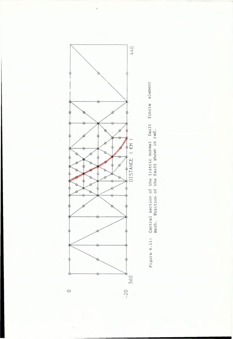
o -4
U 2 < >— CO o
o o to
o o rsj i
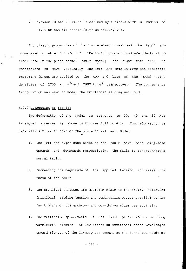
2. Between 10 and 20 km i t i s d e f i n e d by a c i r c l e w i t h a r a d i u s o f
21.25 km and i t s c e n t r e <"x,y) a t ( 4 1 7 . 5 , 0 . 0 ) .
The e l a s t i c p r o p e r t i e s o f t h e f i n i t e element mesh and t h e f a u l t a r e
summarised i n t a b l e s 6.1 and 6.2. The boundary c o n d i t i o n s a r e i d e n t i c a l t o
those used i n t h e p l a n e normal f a u l t model; t h e r i g h t hand s i d e .--as
c o n s t r a i n e d t o move v e r t i c a l l y , t h e l e f t hand edge i s t r e e and i s o s t a t i c
r e s t o r i n g f o r c e s a r e a p p l i e d t o t h e t o p and base o f t h e model u s i n g
d e n s i t i e s o f 2700 kg m"3 and 2900 kg m~3 r e s p e c t i v e l y . The conver g e n c e
f a c t o r w h i c h was used t o model t h e f r i c t i o n a l s l i d i n g was 15.0.
6.2.2 D i s c u s s i o n o f r e s u l t s
The d e f o r m a t i o n o f t h e model i n response t o 30, 40 and 50 MPa
t e n s i o n a l s t r e s s e s i s shown i n f i g u r e s 6.12 t o 6.14. The d e f o r m a t i o n i s
g e n e r a l l y s i m i l a r t o t h a t o f t h e p l a n e normal f a u l t model:
1. The l e f t and r i g h t hand s i d e s o f t h e f a u l t have been d i s p l a c e d
upwards and downwards r e s p e c t i v e l y . The f a u l t i s c o n s e q u e n t l y a
normal f a u l t .
2. I n c r e a s i n g t h e magnitude o f t h e a p p l i e d t e n s i o n i n c r e a s e s t h e
t h r o w o f t h e f a u l t .
3. The p r i n c i p a l s t r e s s e s a r e m o d i f i e d c l o s e t o t h e f a u l t . F o l l o w i n g
f r i c t i o n a l s l i d i n g t e n s i o n and compression o c c u r s p a r a l l e l t o t h e
f a u l t p l a n e on i t s u p t h r o w n and downthrown s i d e s r e s p e c t i v e l y .
4. The v e r t i c a l d i s p l a c e m e n t s a t t h e f a u l t p l a n e i n d u c e a l o n g
w a v e l e n g t h f l e x u r e . At low s t r e s s an a d d i t i o n a l s h o r t w a v e l e n g t h
upward f l e x u r e o f t h e l i t h o s p h e r e o c c u r s on t h e downthrown s i d e o f
- 113 -
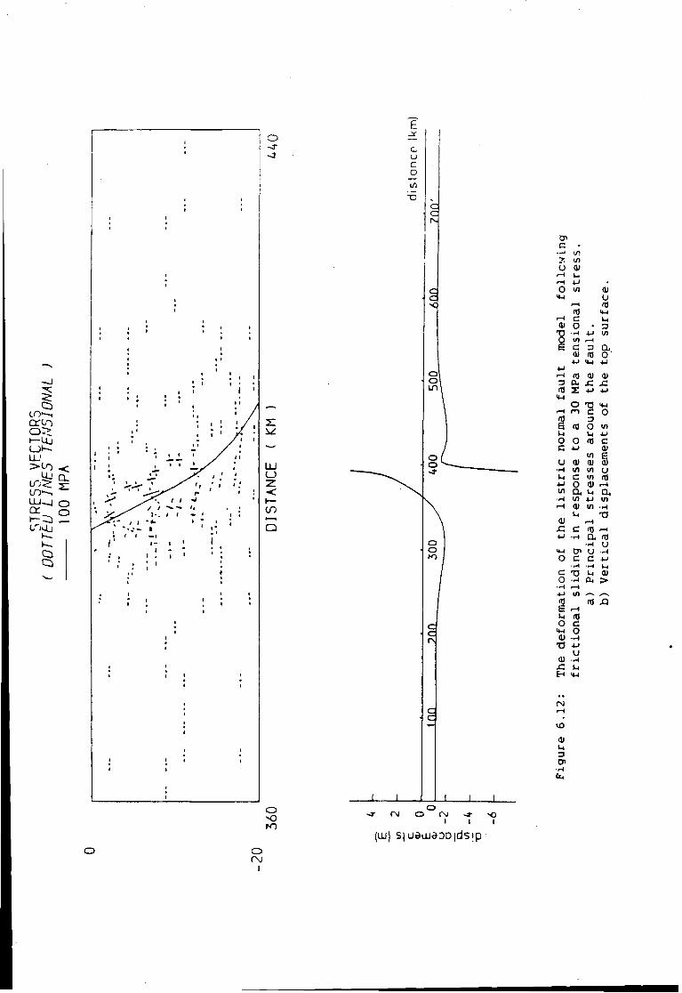
•< Q .
L O - — .
O
Q>
-
o -4
2 :
o < t o
Q
c • —1 1/1 •> i/l 0 &> <-< u
4 J • 0 1/1 (1)
<4-l u »—(
t- l c 1-1
0) 0 • D 32 • - 4 4 J V) 0 V) 1—1 E C 3 a
(1) OJ O ' u <4-l 4-1
4-< 1—t m a) 3 a . . c m
H | 4-1 4-1
0 T3 <*-i r-l m C 0 IS 3 a <tl O in u u 4-1
0 O (0 C c 4-1
in u 01 HI
•-4. VI in u kl C in (0
4-1 0 <U r- l t/1 a u a •w in 4-1 in
<U VI • H T3
QJ r-4 JC C 1—1 4-1 • H nl
U X-l CP u • H O c c 4 J
• r 4 •rH u C XJ O • H 04 > •H »-4
4-1 V) / N <g (0 £; f—1 U (0 O c
<M 0 0) • H
- o 4 J u
0) • H
<*-!
0) u
O
r o 1 1
(uu) s jueujeoDids ip o 0 0 1
o e -X u c o
o o
o o
o - o to
o CM
i
o o i n — i n o i n — —
i i i
(LU) s }uewa3D |ds ip
cn c • 2 ui O 0)
O ul
m c o
T ) •-1 4->
O "1 <-i Ul C 3 0> 0} 4-1 "4-4
0) u ITS
1-1
Ul
a o
3 04
>4-l o
i—* E (3 u O O C 4 J
U 01 -J u) l-i c 4-J 0 <n a
in .-( a)
u
<u at x : x:
01 a) U> (J ui m 0)
O C - H
C TJ O
f-H 4-1 Ul ft} B r-t u ns O C >w o at - H
• a 4 - J u
x: u
a 4-1 Ul Ul
1—1 rrj >-i a f0
• H U U w C 4->
• H 1-1 u a) 04 >
(0 XI
at 1-4 3 Oi
- H
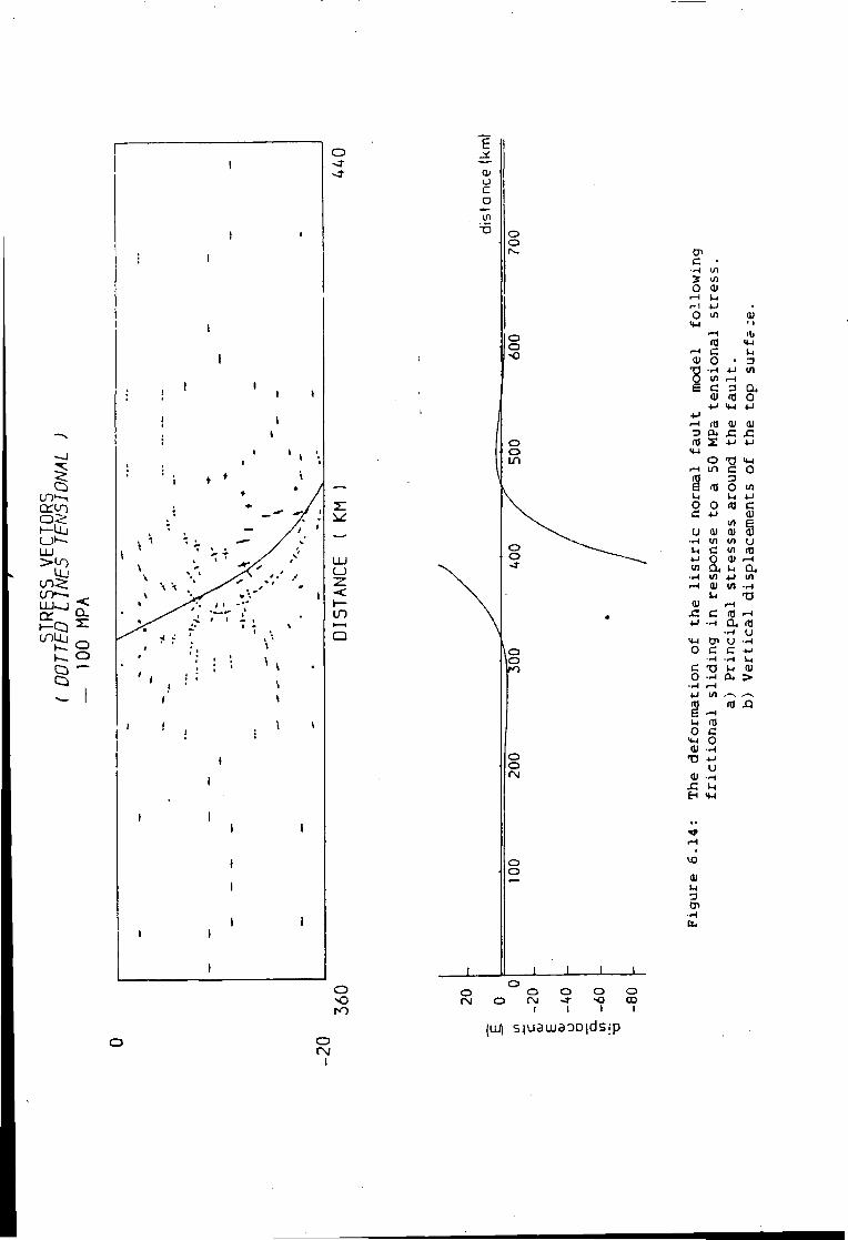
o
i »
i !
e O c o in T5 o
o
o o
o o in
o o
o o CM
o o
o -o o
o o Cst O CM
o S3
o 03
O (M I
(uJ ) s j u a u j a o D i d s i p
c •H i/l s l/l o 01 i—1 r-l 4J • o H )
l/l 0) r-l III m
i—1 c Li 01 0 • 3
13 •i-t 4-1 l/l 0 l/l i-H e c 3 Q-.
01 "3 O 4-> <t-4 4-1
*J i-i m 01 01 3 x: c <0 X 4-1 4-1
o <4-l i—i m c o <S 3 E m o Ul Li Li 4-1 O o (0 c a 4-> 01
l/l e u 0) 0) S •r4 in l/l u U C i/l m 4-1 0 0) i—i l/l a Li a , r4 in 4-1 l/l r-4 01 l/l •i-4
Li T3 01 rH
C 10 •-I 4-1 -.-1 CU (0
•r4 o <4J CP u •H o c c 4-1
•H •H Li c T) Li 0) o •.-1 Q. > •1-1 •-I 4-1 i/l nj ro XI e i-H u O c U-l o 01 •H
Tf 4-1 u
01 x: M
01 u 3 CP
t h e f a u l t . T h i s f l e x u r e , which has i t s a x i s 15 km fr o m t h e f a u l t
p l a n e , d i s a p p e a r s as t h e a p p l i e d t e n s i o n a l s t r e s s i s i n c r e a s e d .
5. I n c r e a s i n g t h e t e n s i o n a i s t r e s s i n c r e a s e s t h e d e p t h t o which
f r i c t i o n a l s l i d i n g o c c u r s . At 30 MPa f r i c t i o n a l s l i d i n g o c c u r s
down t o 10 km, w h i l s t a t 50 MPa i t extends t h r o u g h o u t t h e e l a s t i c
l a y e r . T h i s means t h a t i n c r e a s i n g l y more d e f o r m a t i o n o c c u r s on
the l i s t r i c s e c t i o n o f t h e f a u l t as t h e t e n s i o n i n c r e a s e s .
The v e r t i c a l d i s p l a c e m e n t s i n t h e l i s t r i c f a u l t model a r e c o n s i s t e n t l y
l e s s t h a n t h o s e o f t h e c o r r e s p o n d i n g p l a n e normal f a u l t model. T h i s i s
because r o t a t i o n has t o oc c u r on t h e i i s t r i c f a u l t p l a n e t o m a i n t a i n i t s
geometry.
6.3 T h r u s t F a u l t s
The p r e v i o u s s e c t i o n s o f t h i s c h a p t e r have shown t h a t t h e model o f
f r i c t i o n a l s l i d i n g can s i m u l a t e t h e d e f o r m a t i o n on p l a n e and l i s t r i c n o r m a l
f a u l t s . I n t h i s s e c t i o n t h i s a n a l y s i s i s extended t o model t h e d e f o r m a t i o n
on p l a n e and l i s t r i c t h r u s t f a u l t s .
6.3.1 Plane t h r u s t f a u l t s
The c e n t r a l s e c t i o n o f t h e 1000 km l o n g f i n i t e element mesh and t h e
p o s i t i o n o f t h e p l a n e t h r u s t f a u l t a r e shown i n f i g u r e 6.15. The t h r u s t
f a u l t has a d i p o f 26.57 d e g r e e s . The e l a s t i c p r o p e r t i e s o f t h e f i n i t e
element mesh and t h e f a u l t i r e summarised i n t a b l e s 6.1 and 6.2. The
boundary c o n d i t i o n s which were a p p l i e d t o t h i s body were i d e n t i c a l t o t h o s e
used i n t h e normal f a u l t models ( s e c t i o n 6.2.1).
- 114 -
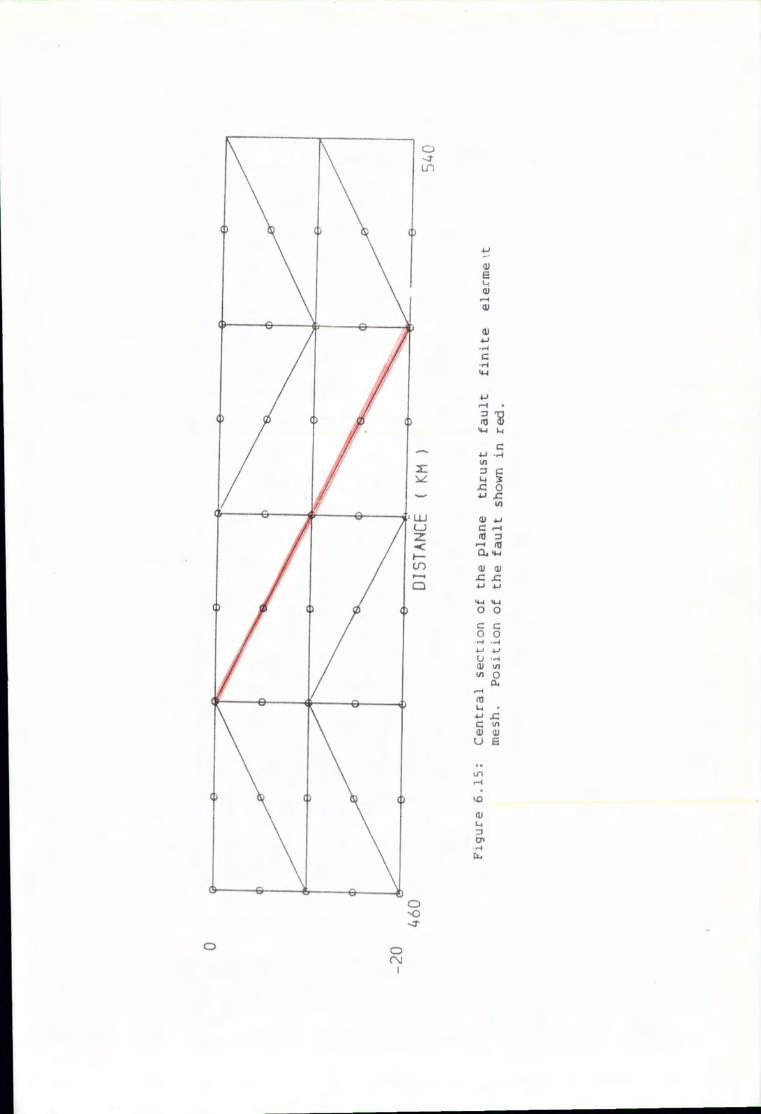
o • J -
e 0)
4-1
•H c
3 TJ fO 5) H-4 1_|
C
4-1 -iH
3 p . c o 4J sz
Ul 4-J
c i 3 r-i
•U t-i OJ 0 £ 4-J
't-l >4-4
o O c c o o
•H -4 4-J u OJ (/) 1/1 o
a, rd
• 4-1
c u i
111 1-1
01
o CM I
The i n i t i a l e l a s t i c d e f o r m a t i o n o f t h e model i n response t o a 30 MPa
compressive s t r e s s i s shown i n f i g u r e 6.16. The t o p s u r f a c e o f t h i s model
t o t h e l e f t and r i g h t hand s i d e s o f t h e f a u l t i s d i s p l a c e d upwards and
downwards r e s p e c t i v e l y . The f a u l t i s c o n s e q u e n t l y a t h r u s t f a u l t . T h i s
t y p e o f f a u l t would be e x p e c t e d t o d e v e l o p i n response t o h o r i z o n t a l
c o m pressive s t r e s s (Anderson, 1951). The e f f e c t of t h e s e l o c a l
d i s p l a c e m e n t s a l o n g t h e f a u l t p l a n e i s t o i n d u c e a l o n g w a v e l e n g t h f l e x u r e
i n t h e a d j a c e n t l i t h o s p h e r e . T h i s e f f e c t has been p r e v i o u s l y o b s e r v e d i n
t h e normal f a u l t models.
The d e f o r m a t i o n f o l l o w i n g f r i c t i o n a l s l i d i n g on t h e f a u l t i s shown i n
f i g u r e 6.17. The f o l l o w i n g g e n e r a l i s a t i o n s can be made fr o m an a n a l y s i s o f
these r e s u l t s :
1. The r e l a t i v e v e r t i c a l d i s p l a c e m e n t s a t t h e f a u l t p l a n e a r e
i n c r e a s e d by f r i c t i o n a l s l i d i n g .
2. The s t r e s s c l o s e t o t h e f a u l t i s m o d i f i e d by t h e f r i c t i o n a l
s l i d i n g . T e n s i o n o c c u r s p a r a l l e l t o t h e f a u l t p l a n e on i t s
o v e r t h r u s t s i d e and compression o c c u r s on i t s d o w n t h r u s t s i d e .
3. A s h o r t w a v e l e n g t h downwards f l e x u r e o f t h e l i t h o s p h e r e o c c u r s on
t h e downthrown s i d e o f t h e f a u l t . T h i s s h o r t w a v e l e n g t h f l e x u r e ,
w h i c h has i t s a x i s 15 km f r o m t h e f a u l t , i s superimposed upon t h e
l o n g w a v e l e n g t h f l e x u r e w h i c h a f f e c t s b o t h s i d e s o f t h e f a u l t . A
s i m i l a r s h o r t w a v e l e n g t h f l e x u r e was o b s e r v e d a t low s t r e s s i n t h e
n o r m a l f a u l t models. T h i s f l e x u r e o c c u r s above t h e f a u l t p l a n e
becau-e f r i c t i o n a l s l i d i n g i s l i m i t e d t o t h e upper p a r t o f t h e
t h r u s t p l a n e .
- 115 -
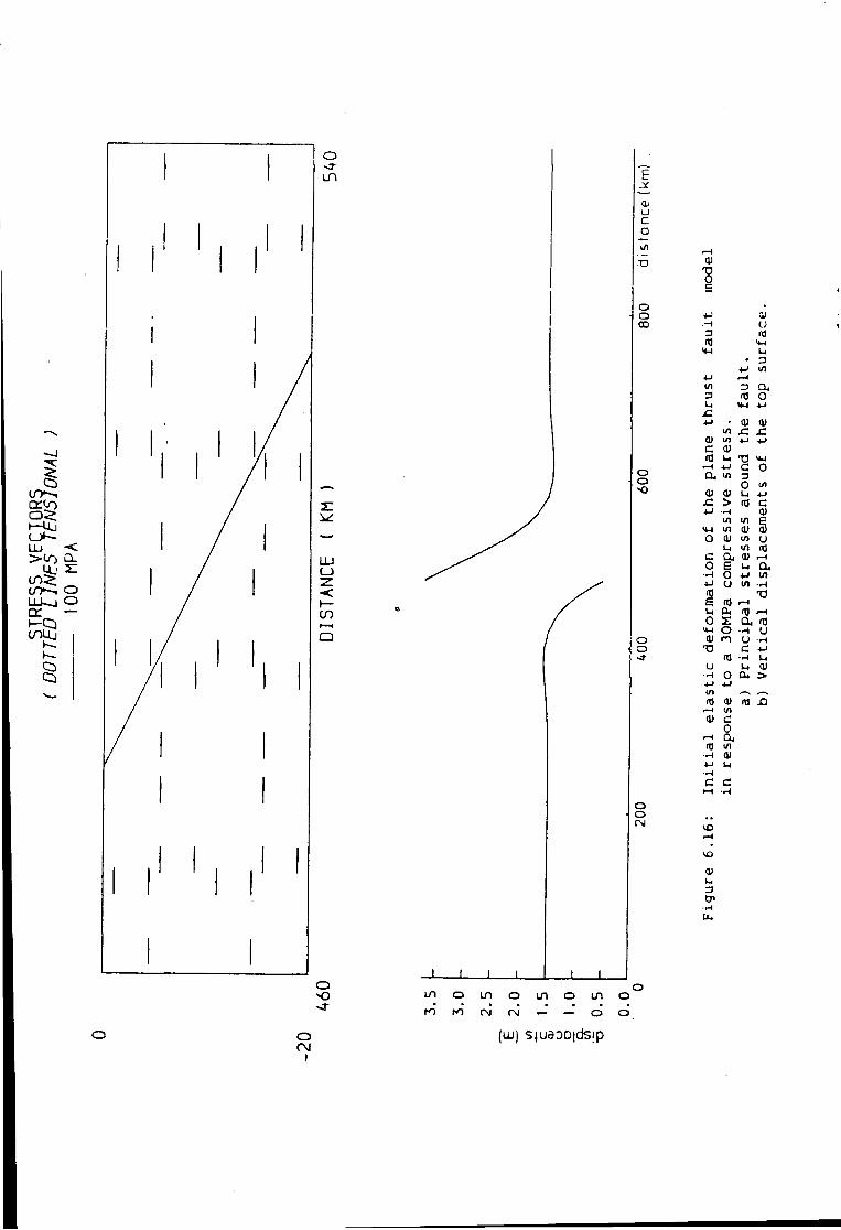
1 cr<-o
<_>-L U • < > t O C L
U j 2= (/>—1 o UJ-J O cr — O T U j
j L _L
O o
ID
O o (M I
( u i ) s } u e o o | d s i p
01
"8
4 J cu .-1 u 3 nJ
4-1 sur
4-1 —4 W 3 a 3 m 0
•4-1 4-1 C 4-1 • 0) o>
1/1 JZ sz 01 l/l 4 J 4-> c 01
u T> W-l i-l 4-1 C 0 a W
no in 0) u 4-1
> td c 4-1
in 1/1 0)
<4-l in o> O 01 in u
u i/j (0 c a, 0) 0 e u a ,
•r4 0 4-» in 4-1 u in •H m X ) e m .-4
X )
IX a) >-H 0 2: a IT]
0 •H U 01 m u •H
T> e 4-> m • H 14
U l-l —1 0 Ou > 4-> 4-1 in ,—, m 0) m XI 1-4 1/1 0)
on
1—1 a , HJ in
01 4 J u c C
•P4
10
ai
3 en [I*
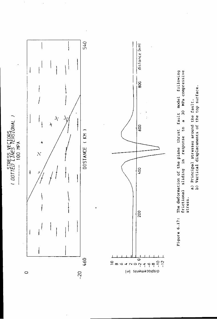
c t r t o
° ^
UJ
co—, U J - J cr »—CTJ COUj
CL
o o
E
o c o
t7> 01 c > .-1 2 1/1 0 1/1 1—1 0) .—I u • o a , 01
s u o <o u 14-4
1—1 U 0> ra • 3 T1 4 J w Q X r—1
3 a ro o
o <4-i 4-1 •u e l •—I 01 3 x : x :
IW (0 4-1 4-1
T3 14-1 O C o
4-1 4-1 3 V) O in 3 u 4-1
a> HJ c w 01
4-1 C m o 0) ol cu in u
0) in in 10 c at 01 f—1 m U a ,
r-4 * J in a in
c TD i-i
x: rfl .-4. 4-1 a< (0
CP •H U <4-4 c U •H o •H c 4-1
T3 1-4 c —4 01 o r-l cu > •iH in 4-1 —*
XJ i-H
u <a O c
<4-4 o • <u •H w
4-1 in U 01
•rH t-i x : 1-1 4-1
4-1 in
i a
a*
3 0>
o CM
I
(ui) s^aaiaoD|dsip
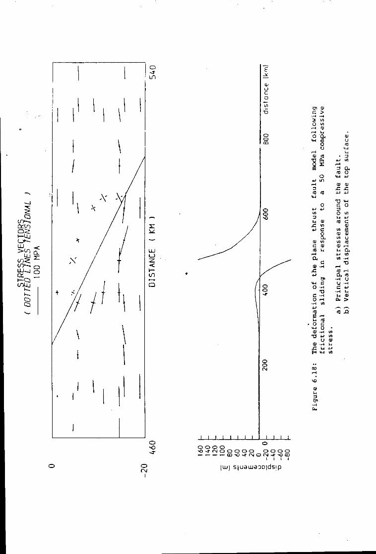
— I
Q CO-, o> H - U j O -LU « c
C O 1 — 0
•-p ~" COUj
8
E
o> o c o
o o 00
I I I 1 1 _L_L
o o
o o
o o CM
1 1 1 1 o o o o • o - r r s i o o o o o o o o o — • -OOOJ-(MO(M-JOCD
I I I I
01 0) C > •H •1-1
3 l/l O l/l
•—1 D r-4 t-i • o O , 01
>4-l
co
m
u H-l
i-l u 01 m • 3 V 4-1 Ul
0 X i-l 6
o
3 m
<4-l top
+ J i n r-l 01 01 3 Xt x : m (0 4-1 4-1
<t-i <4-4
0 C o 4-1 4-> 3 1/1 o l/l 3 l-i 4-1 l_ oi C in 4 J C
a 01 i/l C 01 m u i-l a
e 01 JC u
0> <t-i C O H
T( C -H O rH
•H in
(0 C 0)
ul S oi <D Ul u ui 03 0) «-4
I - I a 4-> Ul
rO .-4
a t> • H U U "H C 4-1
• H L4 Ul 01
O . >
u o 14-1 0) •a 0)
x : H
00
0) 1-4 3
(0 c o •
•H Ul 4-1 l/l U 0)
o Csl I
(UJ) s juaajaoD)dsip
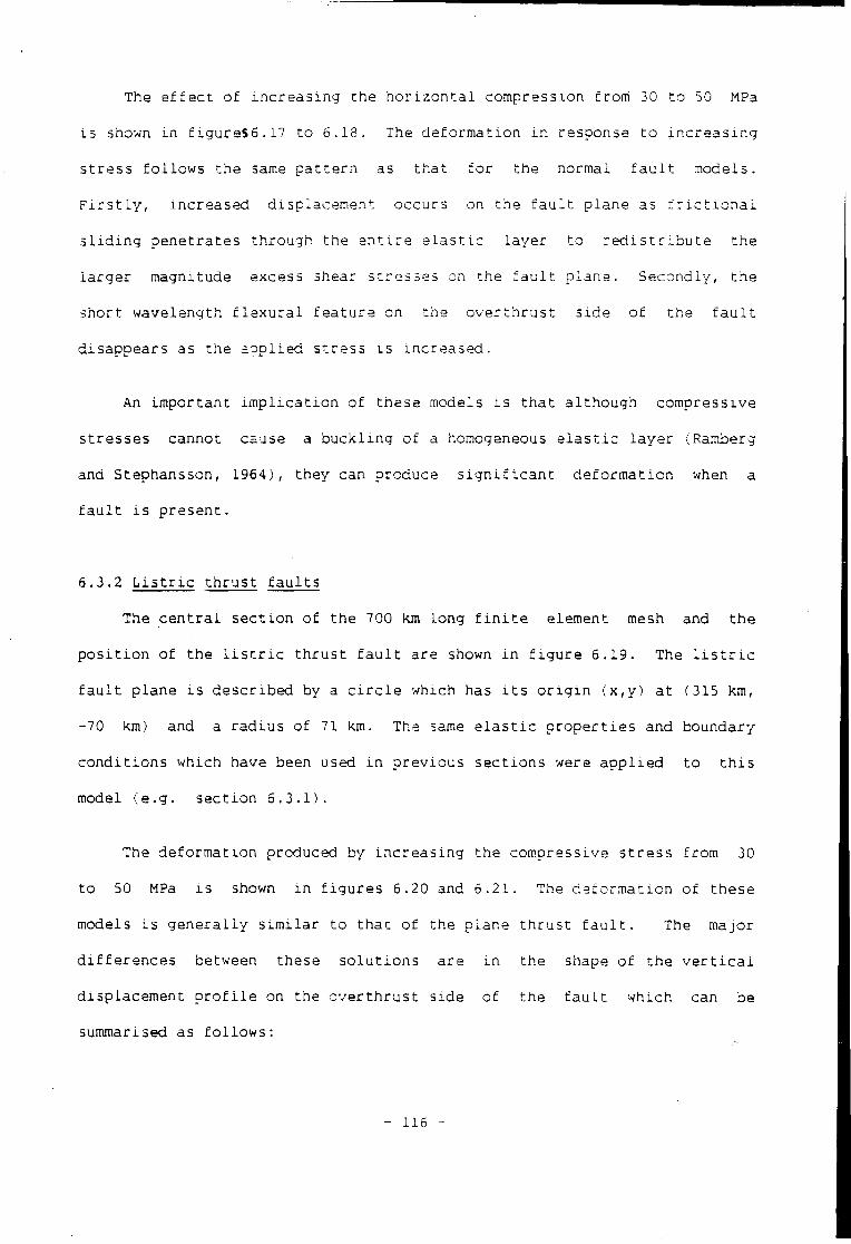
The e f f e c t o f i n c r e a s i n g t h e h o r i z o n t a l c o m p r e s s i o n f r o m 30 t o 50 MPa
15 shown i n f i g u r e S 6 . 1 7 t o 6.18. The d e f o r m a t i o n i n response t o i n c r e a s i n g
s t r e s s f o l l o w s t h e same p a t t e r n as t h a t f o r t h e normal f a u l t models.
F i r s t l y , i n c r e a s e d d i s p l a c e m e n t o c c u r s on t h e f a u l t p l a n e as f r i c t i o n a l
s l i d i n g p e n e t r a t e s t h r o u g h t h e e n t i r e e l a s t i c l a y e r t o r e d i s t r i b u t e t h e
l a r g e r magnitude excess shear s t r e s s e s on t h e f a u l t p l a n e . S e condly, t h e
s h o r t w a v e l e n g t h f l e x u r a l f e a t u r e on t h e o v e r t h r u s t s i d e o f t h e f a u l t
d i s a p p e a r s as t h e a p p l i e d s t r e s s i s i n c r e a s e d .
An i m p o r t a n t i m p l i c a t i o n o f t h e s e models i s t h a t a l t h o u g h c o m p r e s s i v e
s t r e s s e s cannot cause a b u c k l i n g o f a homogeneous e l a s t i c l a y e r (Ramberg
and Stephansson, 1964), t h e y can produce s i g n i f i c a n t d e f o r m a t i o n when a
f a u l t i s p r e s e n t .
6.3.2 L i s t r i c t h r u s t f a u l t s
The c e n t r a l s e c t i o n o f t h e 700 km l o n g f i n i t e element mesh and t h e
p o s i t i o n o f t h e l i s t r i c t h r u s t f a u l t a r e shown i n f i g u r e 6.19. The l i s t r i c
f a u l t p l a n e i s d e s c r i b e d by a c i r c l e which has i t s o r i g i n ( x , y ) a t (315 km,
-70 km) and a r a d i u s o f 71 km. The same e l a s t i c p r o p e r t i e s and boundary
c o n d i t i o n s w h i c h have been used i n p r e v i o u s s e c t i o n s were a p p l i e d t o t h i s
model ( e . g . s e c t i o n 6.3.1).
The d e f o r m a t i o n produced by i n c r e a s i n g t h e c o m p r e s s i v e s t r e s s f r o m 30
t o 50 MPa i s shown i n f i g u r e s 6.20 and 6.21. The d e f o r m a t i o n o f t h e s e
models i s g e n e r a l l y s i m i l a r t o t h a t o f t h e p l a n e t h r u s t f a u l t . The m a j o r
d i f f e r e n c e s between these s o l u t i o n s a r e i n t h e shape o f t h e v e r t i c a l
d i s p l a c e m e n t p r o f i l e on t h e o v e r t h r u s t s i d e o f t h e f a u l t w h i c h can be
summarised as f o l l o w s :
- 116 -
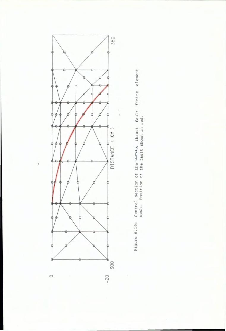
c p V
a • M
fO TJ <4-i 0>
-U C Ul - H 3 Z g *-> O x: VI
? 3 3 <t>
01 01 x: JC
o o c c o o U »H 0) ui ui o ft
r-»
m *-> x: c ui 01 01 U E
H
-o
01 Di
O o (~xJ I
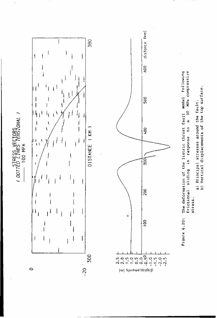
1 i—Lu
>CQ < U j Q=
c r y - , ^
ex. 0
c n u j
I
E
o c o
o o
en 01 c •>
• H S Ul 0 1/1
r-1 0) u •
0 a 0) H-l e u
0 (0 u
r-( u 0) ra • 3 "5 a , 4 J ul 0 X «—1
E a , m 0
0 •4-1 4 J 4-1 n rH 0) 01 3 x :
<*!3 ITJ u 4-1
T3 •4-1
u O C O l/l 4-1 3 3 0 in
1-1 4 J 01 u d Ul 01 C m
u 0 0) o) •H 1/1 u
in IB 4 J 0) 0) r-l 1/1 a ,
-i- l 4- ) l/l r-l 1/1
c •a •-( t~<
£ a) .—1 4-1 cu m
- 4 u c u —1
O c 4.1
t-i c U o> 0 1—1 a , > ••A 1/1
4-> —, (0 X I s i-H l-l 0 c
M-4 0 • d) •H l/l
X) 4-1 Ul u 0)
•H u sz 4-1 H v i 1/1
O
0>
a Di
i n o i n o L n o i n o i n O L n (N(N — — 0 0 0 — — fM(M
1 I I I ! O CM
I (LU) s juamaoDidsjp
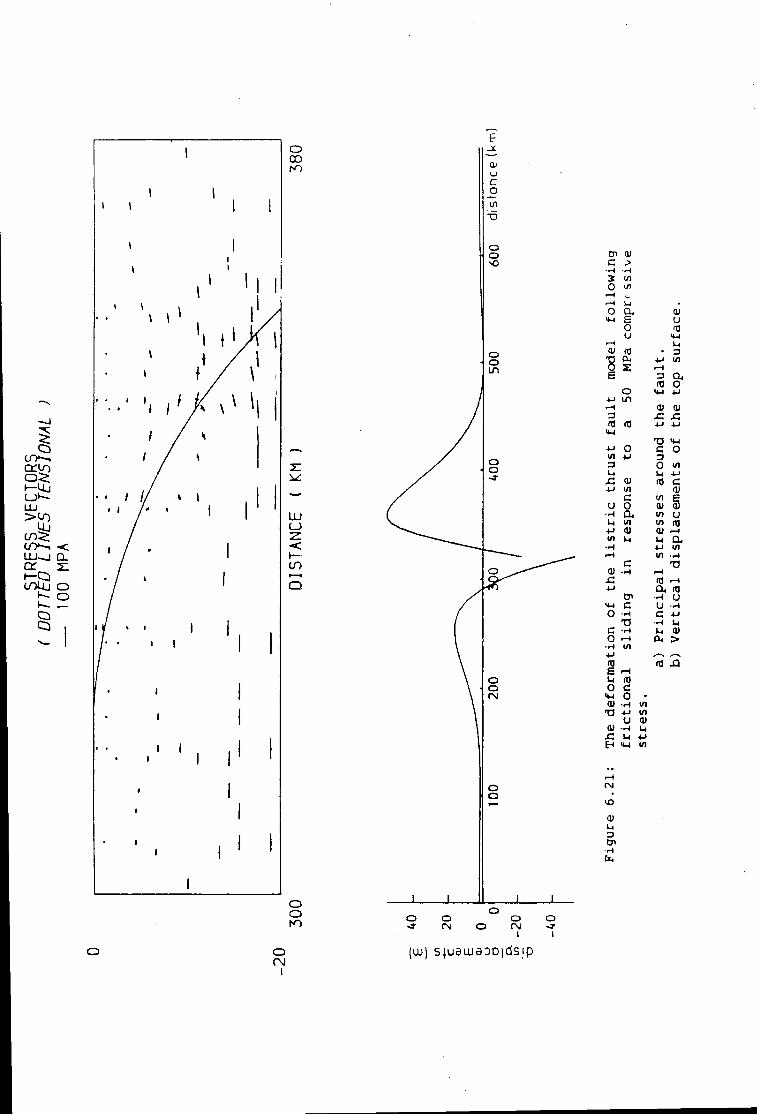
o 0 0
—J
1 t o - - ,
h-U, (_>~ L U
U > - > • < U J - J CL Q: 2;
COUj o
E - X
u c _o in
T5
o o
O o t o
CP Q) c .>
•H —I
0 u> »—( . - I u o a 4-1 E 0
u (V 01
"8 o
4-1 i n
3 1-1
•M in •.-I
43
<n C o a 01 u
01 c
O H T I
C 0 -H • r - | in
I j O
o> T3
0) 43
3 <0
0> U
t-i 3
a , o
0) 01 43 43
t - i C O 3 0 <n i - i 4-1 (fl C
0) 1/1 E 01 <D in u i n m
1- a 4-1 VI 1/1 H
T3
a , 10 •H U U H C 4-1
• ~ l Li U 0) 04 > IT) 43
rtJ c o • H in 4-1 in U 0)
1-1
I O
0> l - i 3
o f M
I
(ui) s } U 5 a i e o D | d s i p
L. Only s e v e r a l metres o f v e r t i c a l d i s p l a c e m e n t o c c u r s a t t h e t o p o f
th e l i s t r i c f a u l t because o f i t s v e r y low a n g l e near t h e s u r f a c e .
2. An upwards f l e x u r e o c c u r s above t h e s t e e p l y d i p p i n g s e c t i o n o f t h e
l i s t r i c f a u l t w h i c h makes t h e s t r e s s e s more t e n s i o n a l a t t h e t o p
o f t h e o v e r t h r u s t l i t h o s p h e r e .
These medals d e m o n s t r a t e t h a t 1: s t r ^ . . ,_..rust f a u l t s can be m o d e l l e d
u s i n g t h e methods o f c h a p t e r 5. The f r i c t i o n a i s l i d i n g model i s t h e r e f o r e
s u i t a b l e f o r a n a l y s i n g t h e d e f o r m a t i o n which o c c u r s on t h e s u b d u c t i o n zone
f a u l t .
6.4 Summary And C o n c l u s i o n s
I n t h i s c h a p t e r t h e p -rformance o f t h e model o f f r i c t i o n a i s l i d i n g
( c h a p t e r 5) has been e v a l u a t e d . The most i m p o r t a n t p o i n t s can be
summarised as f o l l o w s : •
1. The t e s t s have d e m o n s t r a t e d t h a t t h e d u a l node model i s s u i t a b l e
f o r p r e d i c t i n g t h e t y p e o f f a u l t and t h e d e f o r m a t i o n w h i c h i s
produced by f r i c t i o n a i s l i d i n g i n response t o a p p l i e d h o r i z o n t a l
s t r e s s . These r e s u l t s show t h a t t h r u s t f a u l t s a r e p r e d i c t e d i n
response t o c o m p r e s s i o n and normal f a u l t s a r e p r e d i c t e d i n
response t o h o r i z o n t a l t e n s i o n . The model i s c o n s e q u e n t l y
s u i t a b l e f o r p r e d i c t i n g t h e d e f o r m a t i o n w h i c h w i l l o c c u r i n
response t o any s t r e s s regime i f t h e geometry o f t h e f a u l t and i t s
me c h a n i c a l p r o p e r t i e s a r e known o r can be assumed.
2. The model i s c a p a b l e o f a n a l y s i n g t h e d e f o r m a t i o n on b o t h p l a n e
and l i s t r i c f a u l t s .
- 117 -
3. The model p r e d i c t s graben w i d t h s w h i c h a r e comparable w i t h t h e
r e s u l t s w h i c h a r e d e r i v e d from a n a l y t i c t h i n e l a s t i c beam t h e o r y .
The f a i l u r e t o o b t a i n s i m i l a r r e s u l t s w i t h CST elem e n t s ( M i t h e n ,
1980) a r i s e s because t h e f i n i t e element mesh 1 5 t o o s t i f f as an
i n s u f f i c i e n t number o f elements were used t o g i v e a c c u r a t e
s o l u t i o n s t o f l e x u r a l p r o blems. The c o n c l u s i o n s o f M i t h e n ' 3
t h e s i s c o n c e r n i n g t h e f a i l u r e a r i s i n g f r o m l i t h o s p h e r i c f l e x u r e
s h o u l d t h e r e f o r e be used w i t h c a u t i o n u n t i l t h e y have been
v e r i f i e d by co m p a r i s o n w i t h r e s u l t s f r o m i s o p a r a m e t r i c models.
D e s p i t e t h e g e n e r a l success o f t h e model s e v e r a l l i m i t a t i o n s have been
i d e n t i f i e d . F i r s t l y , t h e i t e r a t i v e a l g o r i t h m w h i c h has been used t c model
f r i c t i o n a l s l i d i n g on f a u l t s i s n o t o p t i m a l l y d e s i g n e d . F u t u r e a n a l y s e s
s h o u l d t h e r e f o r e a t t e m p t t o improve t h i s p a r t o f t h e model. Secondly, t h e
p r e d i c t i v e n e s s o f t h e model i s l i m i t e d because t h e v a l u e o f t h e shear
s t i f f n e s s , which c o n t r o l s t h e s c a l e o f t h e f a u l t d e f o r m a t i o n , i s n o t
c o n s t r a i n e d by e x p e r i m e n t a l i n d i c a t i o n s . F u t u r e a n a l y s e s s h o u l d t h e r e f o r e
a t t e m p t t o c o n s t r a i n t h e shear s t i f f n e s s o f f a u l t s by e s t i m a t i n g i t f r o m
r e a l w o r l d examples.
I n c o n c l u s i o n , t h e model which has been d e v e l o p e d i n c h a p t e r 5 i s
c a p a b l e o f m o d e l l i n g f a u l t d e f o r m a t i o n i n a v a r i e t y o f t e c t o n i c s e t t i n g s .
T h i s model w i l l c o n s e q u e n t l y be used i n t h e n e x t c h a p t e r t o a n a l y s e t h e
s t r e s s regime a t s u b d u c t i o n zones.
- 113 -
CHAPTER 7
THE STRESS REGIME AT SUBDUCTION ZONES
7.1 I n t r o d u c t i o n
I n p r e v i o u s c h a p t e r s o f t h i s t h e s i s an i s o p a r a m e t r i c f i n i t e element
method has been d e v e l o p e d w h i c h i s c a p a b l e o f m o d e l l i n g t h e d e f o r m a t i o n
w h i c h o c c u r s a t s u b d u c t i o n zones. I n t h i s c h a p t e r t h i s method i s used t o
model t h e s t r e s s r e g i m e which i s produced a t s u b d u c t i o n zones by l a t e r a l
d e n s i t y v a r i a t i o n s , t h e s l a b p u l l f o r c e , t h e m e c h a n i c a l c o u p l i n g o f t h e
p l a t e s and t h e s l a b i n d u c e d c o n v e c t i o n . The s t r e s s regime p r e d i c t e d by
th e s e models i s t h e n compared w i t h t h e obs e r v e d s t a t e o f s t r e s s a t
s u b d u c t i o n zones t o i n v e s t i g a t e why:
1. A l a t e r a l v a r i a t i o n i n s t r e s s i s o b s e r v e d a c r o s s t h e s t r i k e o f a l l
s u b d u c t i o n zones.
2. The s t a t e o f s t r e s s i n t h e back a r c a r e a o f t h e o v e r l y i n g p l a t e i s
so v a r i a b l e between d i f f e r e n t s u b d u c t i o n zones.
7.2 D e s c r i p t i o n Of The F i n i t e Element Mesh
The f i n i t e element mesh whic h has been used t o model t h e s t r e s s regime
a t s u b d u c t i o n zones i s shown i n f i g u r e 7.1. I t r e p r e s e n t s an i d e a l i s e d two
d i m e n s i o n a l c r o s s s e c t i o n t h r o u g h t h e upper 95 km of an a c t i v e c o n t i n e n t a l
m a r g i n s u b d u c t i o n zone. The f i n i t e element mesh r.as been s i m p l i f i e d by
o m i t t i n g t h e deep s t r u c t u r e o f t h e s u b d u c t i n g p l a t e f r o m t h e model. The
f o r c e s w h i c h a r e t r a n s m i t t e d t o t h e s u r f a c e p l a t e s by t h e subducted o c e a n i c
- 119 -
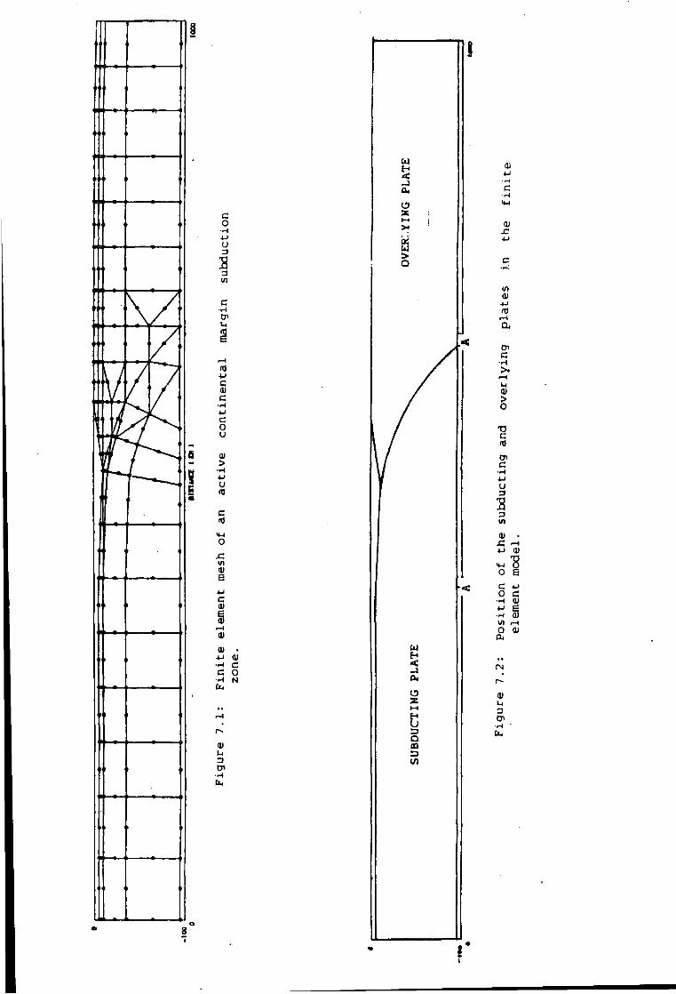
01
01
u 3 s 3
V) 0)
01 01
T3 U
01 C7>
u u 3 s 3 «s i n 01
• J 0)
-8 0)
H 0) 01
O 01 01
w 01 *-> 01
^ N 01
01 HO
in CP
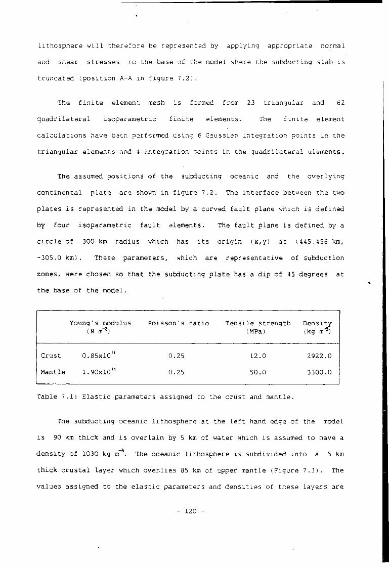
l i t h o s p h e r e w i l l t h e r e f o r e be r e p r e s e n t e d by a p p l y i n g a p p r o p r i a t e normal
and shear s t r e s s e s t o t h e base o f t h e model where t h e s u b d u c t i n g s l a b i s
t r u n c a t e d ( p o s i t i o n A-A i n f i g u r e 7 . 2 ) .
The f i n i t e element mesh i s formed from 23 t r i a n g u l a r and 62
q u a d r i l a t e r a l i s o p a r a m e t r i c f i n i t e e l e m e n t s . The f i n i t e element
c a l c u l a t i o n s have bacn p e r f o r m e d u s i n g 6 Gaussian i n t e g r a t i o n p o i n t s i n t h e
t r i a n g u l a r e l e m e n t s and 4 i n t e g r a t i o n p o i n t s i n t h e q u a d r i l a t e r a l e l e m e n t s .
The assumed p o s i t i o n s o f t h e s u b d u c t i n g o c e a n i c and t h e o v e r l y i n g
c o n t i n e n t a l p l a t e a r e shown i n f i g u r e 7.2. The i n t e r f a c e between t h e two
p l a t e s i s r e p r e s e n t e d i n t h e model by a c u r v e d f a u l t p l a n e w h i c h i s d e f i n e d
by f o u r i s o p a r a m e t r i c f a u l t e l e m e n t s . The f a u l t p l a n e i s d e f i n e d by a
c i r c l e o f 300 km r a d i u s w h i c h has i t s o r i g i n ( x , y ) a t (445.456 km,
-305.0 km). These p a r a m e t e r s , w h i c h a r e r e p r e s e n t a t i v e o f s u b d u c t i o n
zones, were chosen so t h a t t h e s u b d u c t i n g p l a t e has a d i p o f 45 degrees a t
t h e base o f t h e model.
Young's modulus Poisson's r a t i o T e n s i l e s t r e n g t h D e n s i t y (N nf 2) (MPa) ( k g n f 3)
C r u s t 0.85x10" 0.25 12.0 2922 .0
M a n t l e 1.90x10" 0.25 50.0 3300 .0
T a b l e 7.1: E l a s t i c p a r a m e t e r s a s s i g n e d t o t h e c r u s t and m a n t l e .
The s u b d u c t i n g o c e a n i c l i t h o s p h e r e a t t h e l e f t hand edge o f t h e model
i s 90 km t h i c k and i s o v e r l a i n by 5 km o f water which i s assumed t o have a
d e n s i t y o f 1030 kg m"3. The o c e a n i c l i t h o s p h e r e i s s u b d i v i d e d i n t o a 5 km
t h i c k c r u s t a l l a y e r w h i c h o v e r l i e s 85 km o f upper m a n t l e ( F i g u r e 7 . 3 ) . The
v a l u e s a s s i g n e d t o t h e e l a s t i c p a r a m e t e r s and d e n s i t i e s o f t h e s e l a y e r s a r e
- 120 -
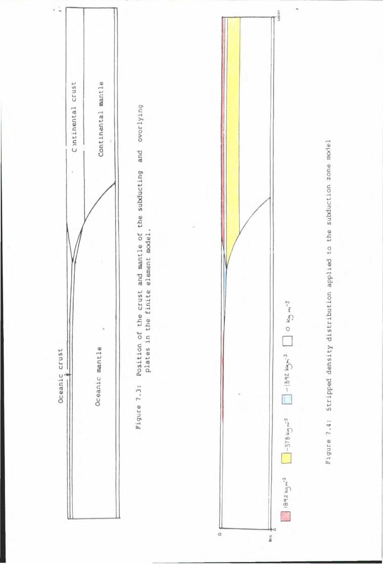
I/] 3 U u 4
C
U
10
c —I
in 3 U u
c 41
a c
<D U O
0i c
CI > o
tjl c
u 3
3 71
<D C
o m 0)
C 4 J
§ § T3 § C n) oi 4-1 01
3 -H l-i C U -H <w 01
J C 01
o c c O i/i •H 01 4 J 4-1 •H ID in ^ O Q, a.
rn
3 CP
15
• M
•
C O
ft I • £ P w tr 00
•
01 c o N c o
u 3 s 3 in D
1 a a a c o
3 A •H M in
•H VI C (1)
-a
r> HI k( 3 CP
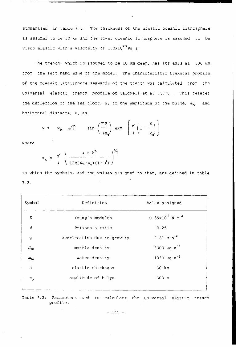
summarised i n t a b l e 7.1. The t h i c k n e s s o f t h e e l a s t i c o c e a n i c l i t h o s p h e r e
i s assumed t o be 30 km and t h e lower o c e a n i c l i t h o s p h e r e i s assumed t o be
23 v i s c o - e l a s t i c w i t h a v i s c o s i t y o f 1.0x10 Pa s.
The t r e n c h , which i s assumed t o be 10 km deep, has i t s a x i s a t 500 km
f r o m t h e l e f t hand edge o f t h e model. The c h a r a c t e r i s t i c f l e x u r a l p r o f i l e
o£ t h e o c e a n i c l i t h o s p h e r a seawards o f t h e t r e n c h was c a l c u l a t e d f r o m the*
u n i v e r s a l e l a s t i c t r e n c h p r o f i l e o f C a l d w e l l e t a] (1976,. T h i s r e l a t e s
t h e d e f l e c t i o n o f t h e sea f l o o r , w, t o t h e a m p l i t u d e o f t h e b u l g e , w b, and
h o r i z o n t a l d i s t a n c e , x, as
w = w b V? • -rrx
s i n | j exp 4x,
where
1Y 4 E h 3
4 \ 1 2 g ( ( o m - / o w ) ( l - I
i n w h i c h t h e symbols, and t h e v a l u e s a s s i g n e d t o them, a r e d e f i n e d i n t a b l e
7.2.
Symbol D e f i n i t i o n Value a s s i g n e d
E Young's modulus 0.85x10" N m~l
\) Poisson's r a t i o 0.25
g a c c e l e r a t i o n due t o g r a v i t y 9.81 m s" 2
m a n t l e d e n s i t y 3300 kg m"3
w a t e r d e n s i t y 1030 kg m"3
h e l a s t i c t h i c k n e s s 30 km
w b a m p l i t u d e o f b u l g e 300 m
T a b l e 7.2: Parameters used t o c a l c u l a t e t h e u n i v e r s a l e l a s t i c t r e n c h p r o f i l e .
- 121 -
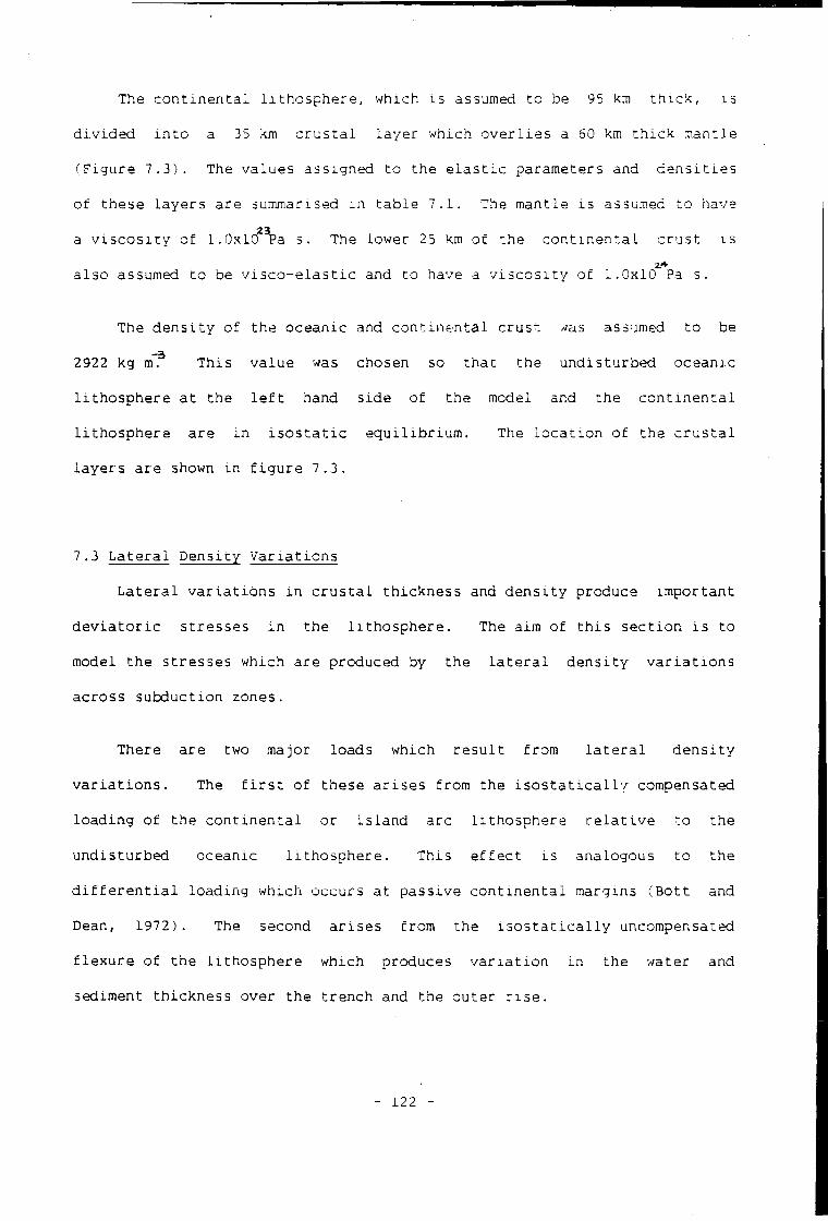
The c o n t i n e n t a l l i t h o s p h e r e , w h i c h i s assumed t o be 95 km t h i c k , i s
d i v i d e d i n t o a 35 km c r u s t a l l a y e r which o v e r l i e s a 60 km t h i c k m a n t l e
( F i g u r e 7 . 3 ) . The v a l u e s a s s i g n e d t o t h e e l a s t i c p a r a m e t e r s and d e n s i t i e s
o f t h e s e l a y e r s a r e summarised i n t a b l e 7.1. The m a n t l e i s assumed t o have
a v i s c o s i t y o f 1.0xl0 2 3Pa s. The lower 25 km o f t h e c o n t i n e n t a l c r u s t i s
a l s o assumed t o be v i s c o - e l a s t i c and t o have a v i s c o s i t y o f 1.0x10 Pa s.
The d e n s i t y o f t h e o c e a n i c and c o n t i n e n t a l c r u s t « s assumed t o be
2922 kg m.3 T h i s v a l u e was chosen so t h a t t h e u n d i s t u r b e d o c e a n i c
l i t h o s p h e r e a t t h e l e f t hand s i d e o f t h e model and t h e c o n t i n e n t a l
l i t h o s p h e r e a r e i n i s o s t a t i c e q u i l i b r i u m . The l o c a t i o n o f t h e c r u s t a l
l a y e r s a r e shown i n f i g u r e 7.3.
7.3 L a t e r a l D e n s i t y V a r i a t i o n s
L a t e r a l v a r i a t i o n s i n c r u s t a l t h i c k n e s s and d e n s i t y produce i m p o r t a n t
d e v i a t o r i c s t r e s s e s i n t h e l i t h o s p h e r e . The aim o f t h i s s e c t i o n i s t o
model t h e s t r e s s e s which a r e produced by t h e l a t e r a l d e n s i t y v a r i a t i o n s
a c r o s s s u b d u c t i o n zones.
There a r e two major l o a d s w h i c h r e s u l t f r o m l a t e r a l d e n s i t y
v a r i a t i o n s . The f i r s t o f t h e s e a r i s e s f r o m t h e i s o s t a t i c a l l y compensated
l o a d i n g o f t h e c o n t i n e n t a l o r i s l a n d a r c l i t h o s p h e r e r e l a t i v e t o t h e
u n d i s t u r b e d o c e a n i c l i t h o s p h e r e . T h i s e f f e c t i s a n a l o g o u s t o t h e
d i f f e r e n t i a l l o a d i n g w h i c h o c c u r s a t p a s s i v e c o n t i n e n t a l m argins ( B o t t and
Dean, 1972). The second a r i s e s f r o m t h e i s o s t a t i c a l l y uncompensated
f l e x u r e o f t h e l i t h o s p h e r e w h i c h produces v a r i a t i o n i n t h e w ater and
sediment t h i c k n e s s o v e r t h e t r e n c h and t h e o u t e r r i s e .
- 122 -
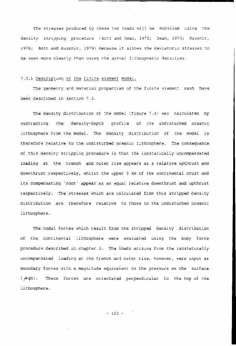
The s t r e s s e s produced by t h e s e two l o a d s w i l l be m o d e l l e d u s i n g t h e
d e n s i t y s t r i p p i n g p r o c e d u r e ( B o t t and Dean, 1972; Dean, 1973; K u s z n i r ,
1976; B o t t and K u s z n i r , 1979) because i t a l l o w s t h e d e v i a t o r i c s t r e s s e s t o
be seen more c l e a r l y t h a n u s i n g t h e a c t u a l l i t h o s p h e r i c d e n s i t i e s .
7.3.1 D e s c r i p t i o n o f t h e f i n i t e element model•
The geometry and m a t e r i a l p r o p e r t i e s o f t h e f i n i t e element mesh have
been d e s c r i b e d i n s e c t i o n 7.2.
The d e n s i t y d i s t r i b u t i o n o f t h e model ( f i g u r e 7.4) was c a l c u l a t e d by
s u b t r a c t i n g t h e d e n s i t y - d e p t h p r o f i l e o f t h e u n d i s t u r b e d o c e a n i c
l i t h o s p h e r e f r o m t h e model. The d e n s i t y d i s t r i b u t i o n o f t h e model i s
t h e r e f o r e r e l a t i v e t o t h e u n d i s t u r b e d o c e a n i c l i t h o s p h e r e . The consequence
o f t h i s d e n s i t y s t r i p p i n g p r o c e d u r e i s t h a t t h e i s o s t a t i c a l l y uncompensated
l o a d i n g a t t h e t r e n c h and o u t e r r i s e appears as a r e l a t i v e u p t h r u s t and
d o w n t h r u s t r e s p e c t i v e l y , w h i l s t t h e upper 5 km o f t h e c o n t i n e n t a l c r u s t and
i t s c o m p e n s a t i n g ' r o o t ' appear as an e q u a l r e l a t i v e d o w n t h r u s t and u p t h r u s t
r e s p e c t i v e l y . The s t r e s s e s w h i c h a r e c a l c u l a t e d f r o m t h i s s t r i p p e d d e n s i t y
d i s t r i b u t i o n a r e t h e r e f o r e r e l a t i v e t o t h o s e i n t h e u n d i s t u r b e d o c e a n i c
l i t h o s p h e r e .
The n o d a l f o r c e s w h i c h r e s u l t f r o m t h e s t r i p p e d d e n s i t y d i s t r i b u t i o n
o f t h e c o n t i n e n t a l l i t h o s p h e r e were e v a l u a t e d u s i n g t h e body f o r c e
p r o c e d u r e d e s c r i b e d i n c h a p t e r 3. The l o a d s a r i s i n g f r o m t h e i s o s t a t i c a l l y
uncompensated l o a d i n g a t t h e t r e n c h and o u t e r r i s e , however, were i n p u t as
boundary f o r c e s w i t h a magnitude e q u i v a l e n t t o t h e p r e s s u r e on t h e s u r f a c e
( /°gh) • These f o r c e s a r e o r i e n t a t e d p e r p e n d i c u l a r t o t h e t o p o f t h e
l i t h o s p h e r e .
- 123 -
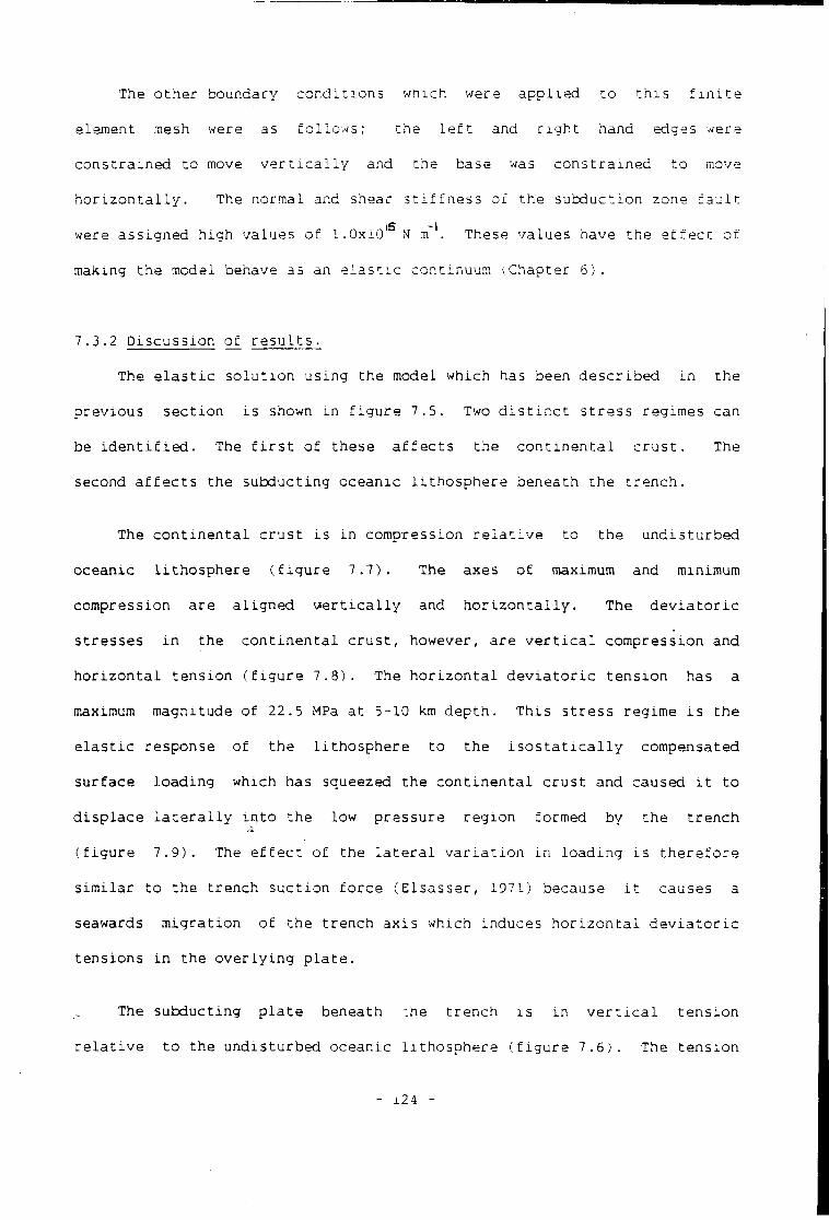
The o t h e r boundary c o n d i t i o n s w h i c h were a p p l i e d to t h i s f i n i t e
element mesh were as f o l l o w s ; t h e l e f t and r i g h t hand edges were
c o n s t r a i n e d t o move v e r t i c a l l y and t h e base was c o n s t r a i n e d to move
h o r i z o n t a l l y . The normal and shear s t i f f n e s s of t h e s u b d u c t i o n zone f a u l t
were a s s i g n e d h i g h v a l u e s of 1 . 0 x l 0 l S N m'. These v a l u e s have t h e e f f e c t of
making t h e model behave as an e l a s t i c c o n t i n u u m ( C h a p t e r 6 ) .
7.3.2 D i s c u s s i o n of r e s u l t s .
The e l a s t i c s o l u t i o n u s i n g t h e model wh i c h has been d e s c r i b e d i n t h e
p r e v i o u s s e c t i o n i s shown i n f i g u r e 7.5. Two d i s t i n c t s t r e s s regimes can
be i d e n t i f i e d . The f i r s t o f t h e s e a f f e c t s t h e c o n t i n e n t a l c r u s t . The
second a f f e c t s t h e s u b d u c t i n g o c e a n i c l i t h o s p h e r e b eneath t h e t r e n c h .
The c o n t i n e n t a l c r u s t i s i n co m p r e s s i o n r e l a t i v e t o t h e u n d i s t u r b e d
o c e a n i c l i t h o s p h e r e ( f i g u r e 7 . 7 ) . The axes o f maximum and minimum
comp r e s s i o n a r e a l i g n e d v e r t i c a l l y and h o r i z o n t a l l y . The d e v i a t o r i c
s t r e s s e s i n t h e c o n t i n e n t a l c r u s t , however, a r e v e r t i c a l c o m p r e s s i o n and
h o r i z o n t a l t e n s i o n ( f i g u r e 7 . 8 ) . The h o r i z o n t a l d e v i a t o r i c t e n s i o n has a
maximum magnitude o f 22.5 MPa a t 5-10 km d e p t h . T h i s s t r e s s r e g i m e i s t h e
e l a s t i c response o f t h e l i t h o s p h e r e t o t h e i s o s t a t i c a l l y compensated
s u r f a c e l o a d i n g w h i c h has squeezed t h e c o n t i n e n t a l c r u s t and caused i t t o
d i s p l a c e l a t e r a l l y i n t o t h e low p r e s s u r e r e g i o n formed by t h e t r e n c h
( f i g u r e 7 . 9 ) . The e f f e c t o f t h e l a t e r a l v a r i a t i o n i n l o a d i n g i s t h e r e f o r e
s i m i l a r t o t h e t r e n c h s u c t i o n f o r c e ( E l s a s s e r , 1971) because i t causes a
seawards m i g r a t i o n o f t h e t r e n c h a x i s which induces h o r i z o n t a l d e v i a t o r i c
t e n s i o n s i n t h e o v e r l y i n g p l a t e .
The s u b d u c t i n g p l a t e beneath :he t r e n c h i s i n v e r t i c a l t e n s i o n
r e l a t i v e t o t h e u n d i s t u r b e d o c e a n i c l i t h o s p h e r e ( f i g u r e 7 . 6 ) . The t e n s i o n
- 124 -
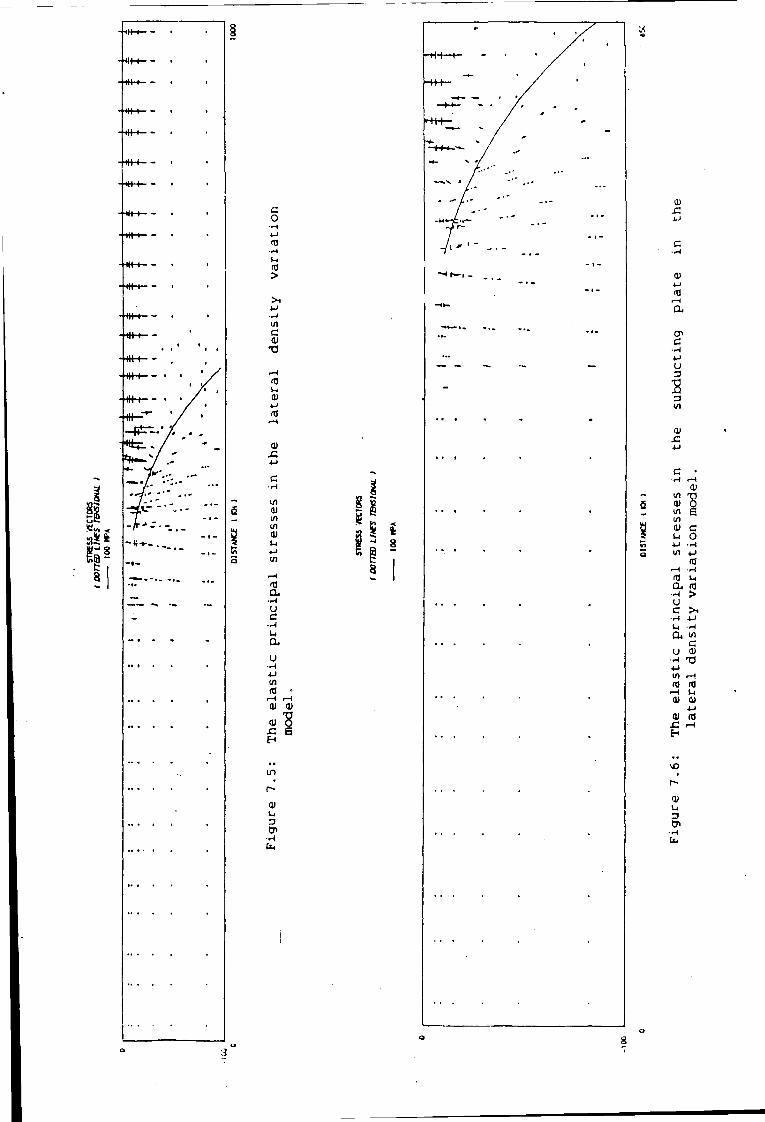
c o
>
• r J U l c
m l - l 01 4-1 m
01 JZ 4->
c • H
l/l 01 l/l U l 01 u 4-> U l
(0 a. u c
•r4 U a. u
• H + J U l m •
.—1 01 0)
rr-i
01 S H
in r-0>
t-l
CP
i -8 I
c . •<-t • - I 0)
U l "0 01 0 i/i s U l 0) c u 0 4-> U l 4->
nj r - l H> U l a.
• H > u c •r-t 4-1
• H Q 4 U l
c u 0) • H T3 4-> U l r H m (0 i-H l - l 01 0>
4-1 01 ia
i-H
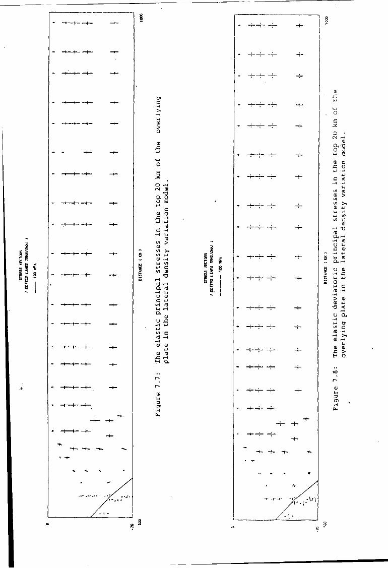
i
CP c
u
> o
0)
H 1 (-
H (-
O r - ( CM 0) a o 1
o e c
a) o
-t ( 1-
C H
HJ V) > 0) in > . in i-J 0) H u V I 4-1 C </> at
T3
a <TJ
U 0) c *-> U r-\
a, u c
8s
8.
H 1 H
v i C (TJ - H
. — I Q) 0)
01 (0 & <-*
i t-
H H
0) 1-4 p
N
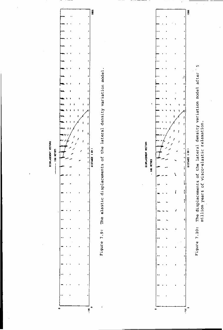
0)
"8 6 C o
l - l
>
in c 0)
T3
m
o in
c
u ITJ
i-H a in
U
in ro
0) C E-t
CM
0) t-i
3 • H
01 4->
0)
"8 e c o 4-1 IT)
> • c
>i o in (tj C *! 0) IT)
01 ft l-i m « u u
Q <J> --4 4-1 4 J (TJ in
• - I (0 f-t a) o> x: i
* j o u t - i i n
m 4-1 c 0> s d) U (TJ
in
(TJ 0) r - i >i a, in c H O T3 - H
I - I
H S
01 l-l 3
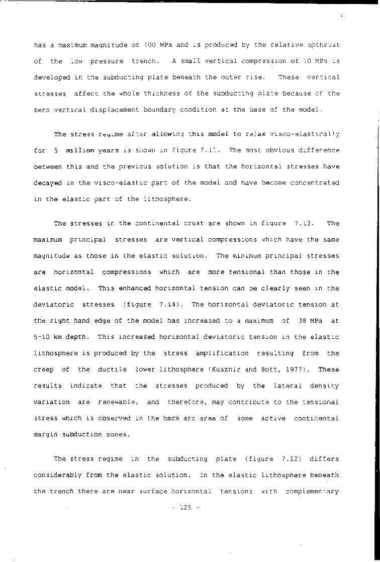
has a maximum magnitude o f 100 MPa and i s produce d by t h e r e l a t i v e u p t h r u s t
o f t h e low p r e s s u r e t r e n c h . A s m a l l v e r t i c a l c o m p r e s s i o n o f 10 MPa i s
de v e l o p e d i n t h e s u b d u c t i n g p l a t e beneath t h e o u t e r r i s e . These v e r t i c a l
s t r e s s e s a f f e c t t h e whole t h i c k n e s s o f t h e s u b d u c t i n g p l a t e because of t h e
ze r o v e r t i c a l d i s p l a c e m e n t boundary c o n d i t i o n a t t h e base o f t h e model.
The s t r e s s r e g i m e a f t e r a l l o w i n g t h i s model t o re J a x v i s c o - e l a s t i c a l l y
f o r 5 m i l l i o n y e a r s i s shown i n f i g u r e 7.1.\. The most o b v i o u s d i f f e r e n c e
between t h i s and t h e p r e v i o u s s o l u t i o n i s t h a t t h e h o r i z o n t a l s t r e s s e s have
decayed i n t h e v i s c o - e l a s t i c p a r t o f t h e model and have become c o n c e n t r a t e d
i n t h e e l a s t i c p a r t o f t h e l i t h o s p h e r e .
The s t r e s s e s i n t h e c o n t i n e n t a l c r u s t a r e shown i n f i g u r e 7.13. The
maximum p r i n c i p a l s t r e s s e s a r e v e r t i c a l c o mpressions w h i c h have t h e same
magnitude as t h o s e i n t h e e l a s t i c s o l u t i o n . The minimum p r i n c i p a l s t r e s s e s
a r e h o r i z o n t a l c ompressions w h i c h a r e more t e n s i o n a l t h a n t h o s e i n t h e
e l a s t i c model. T h i s enhanced h o r i z o n t a l t e n s i o n can be c l e a r l y seen i n t h e
d e v i a t o r i c s t r e s s e s ( f i g u r e 7 . 14). The h o r i z o n t a l d e v i a t o r i c t e n s i o n a t
t h e r i g h t hand edge o f t h e model has i n c r e a s e d t o a maximum o f 38 MPa a t
5-10 km d e p t h . T h i s i n c r e a s e d h o r i z o n t a l d e v i a t o r i c t e n s i o n i n t h e e l a s t i c
l i t h o s p h e r e i s produc e d by t h e s t r e s s a m p l i f i c a t i o n r e s u l t i n g f r o m t h e
cre e p o f t h e d u c t i l e lower l i t h o s p h e r e ( K u s z n i r and B o t t , 1 9 7 7 ). These
r e s u l t s i n d i c a t e t h a t t h e s t r e s s e s produced by t h e l a t e r a l d e n s i t y
v a r i a t i o n a r e r e n e w a b l e , and t h e r e f o r e , may c o n t r i b u t e t o t h e t e n s i o n a l
s t r e s s which i s o b s e r v e d i n t h e back a r c a r e a o f some a c t i v e c o n t i n e n t a l
m a r g i n s u b d u c t i o n zones.
The s t r e s s regime i n t h e s u b d u c t i n g p l a t e ( f i g u r e 7.12) d i f f e r s
c o n s i d e r a b l y f r o m t h e e l a s t i c s o l u t i o n . I n t h e e l a s t i c l i t h o s p h e r e b e n e a t h
th e t r e n c h t h e r e a r e near s u r f a c e h o r i z o n t a l t e n s i o n s w i t h complementary
- 125 -
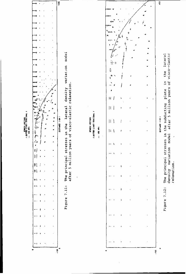
r *
i s
HI <
i i \
0>
V 0 e
c o
w m
• rH
M (0 > •
C o
• H
-M 4-1 • H (0 </l X C m d) i—1
X3 01 l-l
f-H u (0 • H
l-l +J <u U 1
(0 r—1
r-H 01 1
o 0> u
( / I 4-1
> c - 4 .
o 1/1
01 i n 1/1 u 1/1 aj 0> 0> L i > i
4->
i/l c o
i -H •l-l (0 1—1
CL l - l • I H • H
u e c
i n u a , i-i
0) <u u c <t-i
m
01 L-l 3 en
• H
§ § 3 .
II 1
11 \
5
1—1 u rtj •H 1H 4-1 OJ 1/1
4 J m m i—i i—i c
1 o
01 u JC 1/1 4-1 • H
> c <»-l
• H o i n
0> 4-1 (0 (0 01
l - l >1 a c 0
en • H
c l - l - H l - l 4 J • H U
s 73 u 1/1 01
4 J 01 > w
x ; «J 4->
c i—i • l - l 01
l / l
0< e 1/1 1/1 <U c l j o
4 J • H U l 4 J
a) f—t • H
m l-l a , •
• H > C u o c • l - l
> 1 4 -1 u 4 J n) Cu • H X
i n (0 01 c i - l
0> 0> T 3 l-l
01 u D
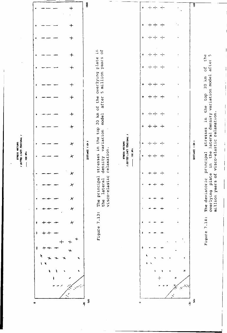
+
+
+
+
+
-+--+- Jr
- + - H — - V -
+ H — i -
+ + +
^ % - i - -y. x
c * - i —1 0
<D in *-J
(13 m r - l 01 a ,
cn c c o •A • H >1 r - l
r - l r—1 -<
0) e > 0 i n
u c 0)
4-1
rd o
e r-H
a; o CM e a , o c 4 J o
•r-1
0) 4->
sz nj u • H
i-i c in «
•r-1 > c o
l / l
QJ >• 4 J
i/i <tl i/i - i X 0) in ro i-i C r-4
u ai ai i/i T> u
r—( u r - 1 • H
a , «3 4 J L l 1/1
(J a> rfl c • P r -H
(0 0 ) U > - i 1
a , o u
(U 0) in . c c H 4 J >
0) L l a
+ -7-
•t \
1 >l
ai in
-M i-i 0) u
U-l <*-i
0 rtj i—i
e "8
o £ c o
a , • H o 4-1
4-1 m • H U
Q j m C > 4 J •
> c 4-i 0
c • W -<H
•1-1 l/l 4-1
C nj Q)
l/l T 3 03 CD r - l i/l r-H 0) i/l a) I-I 0) u u 0) u
4-1 4 J • rH
l/l IT) 4-1
—1 in
r - l 0> r-H
<D IX 4 J 1
• r - | O U U C c l/l r-* -r-1 1-1 > a
0) 4-1 O
u rtj • H r - 1 t / i
u a I-I o n) 4-1 a) (0 >*
•H c > r-l c aj >! 0 TJ i—1 •-i
1-1 r - l 0) r - l -c > • r 4
H o e
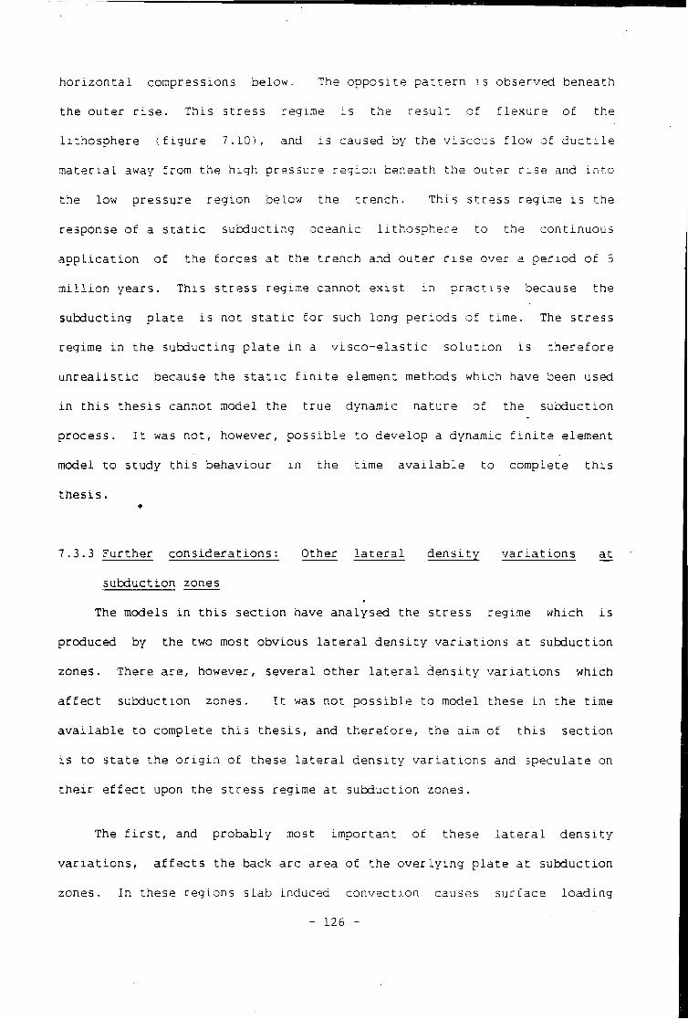
h o r i z o n t a l c ompressions below. The o p p o s i t e p a t t e r n i s o b s e r v e d b e n e a t h
th e o u t e r r i s e . T h i s s t r e s s regime i s t h e r e s u l t o f f l e x u r e o f t h e
l i t h o s p h e r e ( f i g u r e 7.10), and i s caused by t h e v i s c o u s f l o w o f d u c t i l e
m a t e r i a l away from t h e h i g h p r e s s u r e r e g i o n beneath t h e o u t e r r i s e and i n t o
t h e low p r e s s u r e r e g i o n below t h e t r e n c h . T h i s s t r e s s regime i s t h e
response o f a s t a t i c s u b d u c t i n g o c e a n i c l i t h o s p h e r e t o t h e c o n t i n u o u s
a p p l i c a t i o n o f t h e f o r c e s a t t h e t r e n c h and o u t e r r i s e over a p e r i o d o f 5
m i l l i o n y e a r s . T h i s s t r e s s regime cannot e x i s t i n p r a c t i s e because t h e
s u b d u c t i n g p l a t e i s n o t s t a t i c f o r such l o n g p e r i o d s o f t i m e . The s t r e s s
regime i n t h e s u b d u c t i n g p l a t e i n a v i s c o - e l a s t i c s o l u t i o n i s t h e r e f o r e
u n r e a l i s t i c because t h e s t a t i c f i n i t e element methods which have been used
i n t h i s t h e s i s cannot model t h e t r u e dynamic n a t u r e o f t h e s u b d u c t i o n
p r o c e s s . I t was n o t , however, p o s s i b l e t o d e v e l o p a dynamic f i n i t e element
model t o s t u d y t h i s b e h a v i o u r i n t h e t i m e a v a i l a b l e t o c o m p l e t e t h i s
t h e s i s . 9
7.3.3 F u r t h e r c o n s i d e r a t i o n s : Other l a t e r a l d e n s i t y v a r i a t i o n s a t
s u b d u c t i o n zones
The models i n t h i s s e c t i o n have a n a l y s e d t h e s t r e s s regime w h i c h i s
produced by t h e two most o b v i o u s l a t e r a l d e n s i t y v a r i a t i o n s a t s u b d u c t i o n
zones. There a r e , however, s e v e r a l o t h e r l a t e r a l d e n s i t y v a r i a t i o n s w h i c h
a f f e c t s u b d u c t i o n zones. I t was n o t p o s s i b l e t o model t h e s e i n t h e t i m e
a v a i l a b l e t o c o m p l e t e t h i s t h e s i s , and t h e r e f o r e , t h e aim o f t h i s s e c t i o n
i s t o s t a t e t h e o r i g i n o f t h e s e l a t e r a l d e n s i t y v a r i a t i o n s and s p e c u l a t e on
t h e i r e f f e c t upon t h e s t r e s s regime a t s u b d u c t i o n zones.
The f i r s t , and p r o b a b l y most i m p o r t a n t o f t h e s e l a t e r a l d e n s i t y
v a r i a t i o n s , a f f e c t s t h e back a r c a r e a o f t h e o v e r l y i n g p l a t e a t s u b d u c t i o n
zones. I n t h e s e r e g i o n s s l a b i n d u c e d c o n v e c t i o n causes s u r f a c e l o a d i n g
- 126 -
w h i c h i s i s o s t a t i c a l l y compensated by a h o t , low d e n s i t y r e g i o n i n t h e
u n d e r l y i n g l i t h o s p h e r e . T h i s l o a d would be e x p e c t e d t o p r o d u c e h o r i z o n t a l
d e v i a t o r i c t e n s i o n s which would be a m p l i f i e d i n a way analogous t o t h o s e i n
r e g i o n s o f p l a t e a u u p l i f t ( B o t t and K u s z n i r , 1979). S i n c e t h e s e s t r e s s e s
a r e renewable t h i s l o a d i n g i s p o t e n t i a l l y i m p o r t a n t i n p r o d u c i n g t h e
o b s e r v e d t e n s i o n a l s t r e s s e s i n back a r c r e g i o n s .
The second l a t e r a l d e n s i t y _ a t i o n a f f e c t s t h e c r u s t b eneath the.
v o l c a n i c a r c . I n t h i s r e g i o n t h e s h o r t w a v e l e n g t h s u r f a c e l o a d o f t h e
v o l c a n i c a r c i s compensated by an u n d e r l y i n g , h o t low d e n s i t y r e g i o n . The
e f f e c t o f t h i s l o a d would be t o produce h o r i z o n t a l d e v i a t o r i c t e n s i o n s i n
t h e c r u s t beneath t h e v o l c a n i c e d i f i c e ( B o t t , 1971). T h i s l o a d c o u l d
t h e r e f o r e be i m p o r t a n t i n l o c a l l y m o d i f y i n g t h e r e g i o n a l s t r e s s r e g i m e , and
c o n s e q u e n t l y , i t may be an i m p o r t a n t f a c t o r i n e x p l a i n i n g t h e o b s e r v a t i o n
t h a t t e n s i o n a l f a i l u r e o c c u r s a t t h e v o l c a n i c a r c d u r i n g t h e i n i t i a t i o n o f
back a r c s p r e a d i n g .
The t h i r d l a t e r a l d e n s i t y v a r i a t i o n w h i c h has been n e g l e c t e d a f f e c t s
t h e back a r c a r e a o f t h e o v e r l y i n g p l a t e a t a c t i v e c o n t i n e n t a l m a r g i n s .
T h i s i s produced by t h e s u r f a c e l o a d i n g o f a c o r d i l l e r a n m o u n t a i n range and
t h e u p t h r u s t o f t h e low d e n s i t y r o o t which compensates t h e l o a d . The
e f f e c t o f t h i s l o a d i n g would be t o produce a d d i t i o n a l h o r i z o n t a l d e v i a t o r i c
t e n s i o n s i n t h e c r u s t b eneath t h e m o u n t a i n range, and t h e s e would be
superimposed upon t h e s t r e s s e s which have been m o d e l l e d i n t h i s s e c t i o n .
7.3.4 L i m i t a t i o n s o f t h e models
There a r e s e v e r a l l i m i t a t i o n s o f t h e models which have been d e v e l o p e d .
These a r e :
- 127 -
1. The models have used t h e d e n s i t y s t r i p p i n g a p p r o a c h r a t h e r t h a n
t h e f u l l l i t h o s p h e r i c d e n s i t i e s . The ma]or l i m i t a t i o n o f t h i s
approach i s t h a t i t n e g l e c t s t h e c o n t r a s t i n t h e e l a s t i c
p r o p e r t i e s between t h e h o r i z o n t a l l a y e r s which a r e s t r i p p e d ( P a r k ,
1981). T h i s l i m i t a t i o n , however, i s u n l i k e l y t o have a major
i n f l u e n c e upon t h e r e s u l t s which have been o b t a i n e d .
2. The d e f o r m a t i o n a r i s i n g f r o m t h e l a t e r a l d e n s i t y v a r i a t i o n s a t
i s l a n d a r c s u b d u c t i o n zones has n o t been m o d e l l e d . The r e s u l t s
which have been o b t a i n e d i n t h i s s e c t i o n , however, a r e a p p l i c a b l e
t o i s l a n d a r c s . T h i s i s because a l t h o u g h t h e o v e r l y i n g p l a t e i n
t h e s e r e g i o n s i s m a i n l y o c e a n i c t h e r e i s an i s o s t a t i c a l l y
compensated c r u s t a l l o a d i n t h e v i c i n i t y o f t h e v o l c a n i c a r c .
T h i s l o a d would be e x p e c t e d t o i n d u c e h o r i z o n t a l d e v i a t o r i c
t e n s i o n s i n t h e i s l a n d a r c c r u s t . These t e n s i o n s , however, would
"not e x t e n d i n t o t h e o c e a n i c l i t h o s p h e r e o f t h e back a r c p l a t e a t
i s l a n d a r c s u b d u c t i o n zones.
3. The base o f t h e model has been c o n s t r a i n e d by t h e z e r o v e r t i c a l
d i s p l a c e m e n t boundary c o n d i t i o n . The v e r t i c a l component o f t h e
l o a d a p p l i e d a t t h e upper s u r f a c e o f t h e t r e n c h - o u t e r r i s e has
t h e r e f o r e been i m p l i c i t y b a l a n c e d by e q u i v a l e n t v e r t i c a l b oundary
f o r c e s d i s t r i b u t e d a l o n g t h e base o f t h i s r e g i o n . At s u b d u c t i o n
zones, however, i t would be ex p e c t e d t h a t t h e l o a d s a t t h e t o p
s u r f a c e o f t h e s u b d u c t i n g p l a t e would be b a l a n c e d by a more
l o c a l i s e d system o f v e r t i c a l f o r c e s a r i s i n g f r o m s l a b p u l l . The
zero v e r t i c a l d i s p l a c e m e n t boundary c o n d i t i o n t h e r e f o r e does n o t
c o r r e c t l y model t h e f o r c e d i s t r i b u t i o n a r i s i n g f r o m t h e v e r t i c a l
component o f t h e s l a b p u l l f o r c e and i t a l s o i n h i b i t s b e n d i n g .
- 123 -
4. A f u r t h e r l i m i t a t i o n o f t h e models i s t h a t t h e y p r e d i c t t h a t
h o r i z o n t a l d e v i a t o r i c t e n s i o n i s p r e s e n t t h r o u g h o u t t h e c r u s t o f
t h e o v e r l y i n g p l a t e . T h i s i s i n c o m p a t i b l e w i t h t h e o b s e r v e d
s t r e s s regime a t many s u b d u c t i o n zones and suggests t h a t o t h e r
f o r c e s a c t on t h e o v e r l y i n g p l a t e .
The l i m i t a t i o n s d i s c u s s e d i n p o i n t s 3 and 4 can be m a i n l y overcome by
i n t r o d u c i n g a s l a b p u l l f o r c e t o t h e base o f t h e model T h i s s i t u a t i o n i s
c o n s i d e r e d i n t h e n e x t s e c t i o n .
7.4 Slab P u l l
The s u b d u c t i n g o c e a n i c p l a t e has a l a r g e n e g a t i v e buoyancy because i t
i s c o o l e r , and c o n s e q u e n t l y d e n s e r , t h a n t h e s u r r o u n d i n g m a n t l e and a l s o
because phase t r a n s i t i o n s t o denser m i n e r a l o g i e s a r e e l e v a t e d i n t h e
s u b d u c t i n g p l a t e (McKenzie, 1969; T u r c o t t e and Oxburgh, 1969; Minear and
Toksoz, 1970a,b; Hasebe e t a l , 1970; Toksoz e t a l , 1971, 1973; T u r c o t t e
and S c h u b e r t , 1971, 1973; G r i g g s , 1972; Schubert e t a l , 1 9 7 5 ). The
p o s s i b i l i t y t h a t a component o f t h i s n e g a t i v e buoyancy f o r c e i s t r a n s m i t t e d
a l o n g t h e s u b d u c t i n g o c e a n i c l i t h o s p h e r e t o d r i v e t h e h o r i z o n t a l m o t i o n s o f
t h e s u r f a c e p l a t e s was suggested by E l s a s s e r ( 1 9 6 9 ) . S i n c e t h e n v a r i o u s
i n dependent approaches have d e m o n s t r a t e d t h e i m p o r t a n c e o f t h i s f o r c e ,
known as s l a b p u l l , i n d r i v i n g t h e o b s e r v e d p l a t e m o t i o n s ( F o r s y t h and
Uyeda, 1975; Harper, 1975; Chappie and T u i l i s , 1977; R i c h a r d s o n e t a l ,
1979). A l l o f these s t u d i e s have d e m o n s t r a t e d t h a t o n l y a f r a c t i o n o f t h e
g r a v i t a t i o n a l p o t e n t i a l o f t h e dense s u b d u c t i n g p l a t e i s t r a n s m i t t e d t o
d r i v e t h e m o t i o n s o f t h e s u r f a c e p l a t e s , and t h e r e f o r e t h a t a s u b s t a n t i a l
p a r t o f t h e n e g a t i v e buoyancy f o r c e must be b a l a n c e d by r e s i s t i n g f o r c e s .
The r e s i s t i n g f o r c e s a r i s e from f r i c t i o n a t t h e i n t e r p l a t e shear zone and
- 129 -
from v i s c o u s d r a g a t t h e c o n t a c t o f t h e s u b d u c t i n g l i t h o s p h e r e w i t h t h e
a s t h e n o s p h e r e ( D a v i e s , 1980). The n e t s l a b p u l l f o r c e which i s t r a n s m i t t e d
t o d r i v e t h e s u r f a c e p l a t e m o t i o n s i s t h e r e f o r e e s t i m a t e d t o be o f a
s i m i l a r magnitude t o t h e r i d g e push f o r c e ('Davies, 1983).
D e s p i t e t h e d e m o n s t r a t i o n t h a t t h e s l a b p u l l f o r c e i s i m p o r t a n t i n
d r i v i n g p l a t e m o t i o n s , t h e r a have b^en no d i r e c t a t t e m p t s t o model t h e
s t r e s s regime which t h i s f o r c e produces i n t h e near s u r f a c e p l a t e s a t a
s u b d u c t i o n zone. T h i s i s because t h e aim o f most p r e v i o u s models o f t h e
s l a b p u l l f o r c e has been t o a n a l y s e t h e s t r e s s a t deep and i n t e r m e d i a t e
d e p t h s i n t h e s u b d u c t i n g p l a t e ( S m i t h and Toksoz, 1972; Neugebauer and
8 r i e t m a y e r , 1975).
The aim o f t h i s s e c t i o n i s t h e r e f o r e t o model t h e s t r e s s regime w h i c h
i s p roduced by t h e s l a b p u l l f o r c e i n t h e upper 95 km o f t h e p l a t e s a t a
s u b d u c t i o n zone.
7.4.1 D e s c r i p t i o n o f t h e f i n i t e element model
The f i n i t e element model i s d e s c r i b e d i n s e c t i o n 7.2. The l e f t and
r i g h t hand s i d e s o f t h i s model were c o n s t r a i n e d t o move v e r t i c a l l y . The
base o f t h e model i s assumed t o be u n d e r l a i n by a f l u i d a s t h e n o s p h e r e w i t h
a d e n s i t y o f 3300 kg m.3 I t i s n e c e s s a r y t o i n t r o d u c e t h i s b o u n dary
c o n d i t i o n so t h a t t h e s l a b p u l l f o r c e can be a p p l i e d t o t h e nodes a t t h e
base o f t h e model. The s u b d u c t i o n zone f a u l t was ' l o c k e d ' by a s s i g n i n g is - I
v a l u e s o f 1.0x10 N m t o i t s normal and shear s t i f f n e s s e s .
The s t r i p p e d i e n s i t y d i s t r i b u t i o n ( s e c t i o n 7.3.1) was a p p l i e d t o t h i s
model t o s i m u l a t e t h e l o a d s w h i c h a r e p r o d u c e d by t h e l a t e r a l d e n s i t y
v a r i a t i o n s a t a s u b d u c t i o n zone. A p p l y i n g t h e s e f o r c e s t o a model w i t h t h e
base u n d e r l a i n by a f l u i d has two e f f e c t s . F i r s t l y , the v e r t i c a l f o r c e s
- 130 -
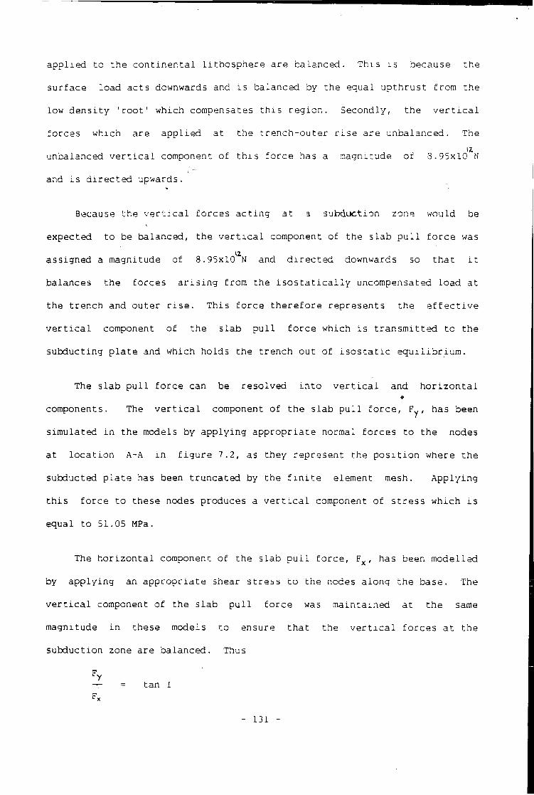
a p p l i e d t o t h e c o n t i n e n t a l l i t h o s p h e r e a r e b a l a n c e d . T h i s i s because t h e
s u r f a c e l o a d a c t s downwards and i s b a l a n c e d by t h e e q u a l u p t h r u s t f r o m t h e
low d e n s i t y ' r o o t ' w h i c h compensates t h i s r e g i o n . Secondly, t h e v e r t i c a l
f o r c e s w h i c h a r e a p p l i e d a t t h e t r e n c h - o u t e r r i s e a r e u n b a l a n c e d . The iz
u nbalanced v e r t i c a l component o f t h i s f o r c e has a magnitude o f 3.95x10 N
and i s d i r e c t e d upwards.
Because t h e v e r t i c a l f o r c e s a c t i n g a t a s u b d u c t i o n zone would be
e x p e c t e d t o be b a l a n c e d , t h e v e r t i c a l component o f t h e s l a b p u l l f o r c e was
a s s i g n e d a magnitude o f 8.95x10 N and d i r e c t e d downwards so t h a t i t
b a l a n c e s t h e f o r c e s a r i s i n g f r o m t h e i s o s t a t i c a l l y uncompensated l o a d a t
t h e t r e n c h and o u t e r r i s e . T h i s f o r c e t h e r e f o r e r e p r e s e n t s t h e e f f e c t i v e
v e r t i c a l component o f t h e s l a b p u l l f o r c e w h i c h i s t r a n s m i t t e d t o t h e
s u b d u c t i n g p l a t e and which h o l d s t h e t r e n c h o u t o f i s o s t a t i c e q u i l i b r i u m .
The s l a b p u l l f o r c e can be r e s o l v e d i n t o v e r t i c a l and h o r i z o n t a l 9
components. The v e r t i c a l component o f t h e s l a b p u l l f o r c e , Fy, has been
s i m u l a t e d i n t h e models by a p p l y i n g a p p r o p r i a t e normal f o r c e s t o t h e nodes
a t l o c a t i o n A-A i n f i g u r e 7.2, as t h e y r e p r e s e n t t h e p o s i t i o n where t h e
subducted p l a t e has been t r u n c a t e d by t h e f i n i t e element mesh. A p p l y i n g
t h i s f o r c e t o these nodes produces a v e r t i c a l component o f s t r e s s w h i c h i s
e q u a l t o 51.05 MPa.
The h o r i z o n t a l component o f t h e s l a b p u l l f o r c e , F , has been m o d e l l e d
by a p p l y i n g an a p p r o p r i a t e shear s t r e s s t o t h e nodes a l o n g t h e base. The
v e r t i c a l component o f t h e s l a b p u l l f o r c e was m a i n t a i n e d a t t h e same
magnitude i n t h e s e models t o ensure t h a t t h e v e r t i c a l f o r c e s a t t h e
s u b d u c t i o n zone a r e b a l a n c e d . Thus
— = t a n I Fx
- 131 -
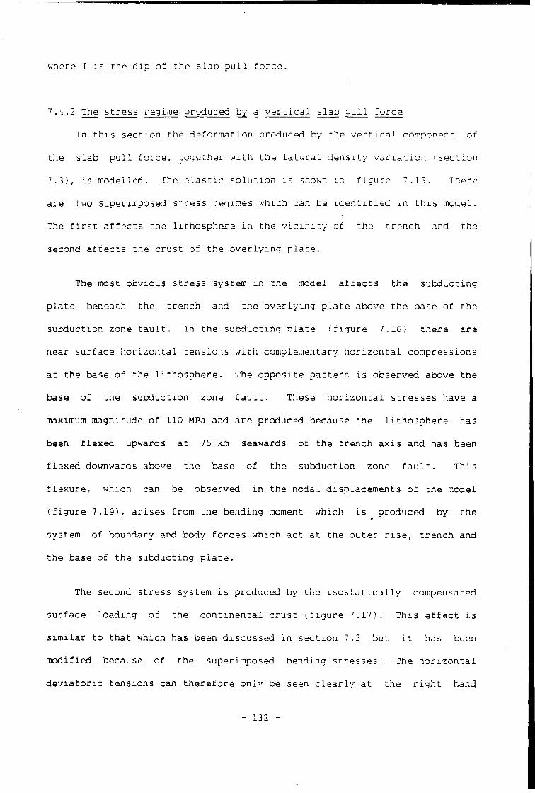
where I i s t h e d i p o f t h e s l a b p u l l f o r c e .
7.4.2 The s t r e s s regime produced by a v e r t i c a l s l a b p u l l f o r c e
I n t h i s s e c t i o n t h e d e f o r m a t i o n produced by t h e v e r t i c a l component o f
t h e s l a b p u l l f o r c e , t o g e t h e r w i t h t h e l a t e r a l d e n s i t y v a r i a t i o n ; s e c t i o n
7 . 3 ) , i s m o d e l l e d . The e l a s t i c s o l u t i o n i s shown i n f i g u r e 7.15. There
a r e two superimposed s t r e s s regimes w h i c h can be i d e n t i f i e d i n t h i s model.
The f i r s t a f f e c t s t h e l i t h o s p h e r e i n t h e v i c i n i t y o f t h e t r e n c h and t h e
second a f f e c t s t h e c r u s t o f t h e o v e r l y i n g p l a t e .
The most o b v i o u s s t r e s s system i n t h e model a f f e c t s t h e s u b d u c t i n g
p l a t e beneath t h e t r e n c h and t h e o v e r l y i n g p l a t e above t h e base o f t h e
s u b d u c t i o n zone f a u l t . I n t h e s u b d u c t i n g p l a t e ( f i g u r e 7.16) t h e r e a r e
near s u r f a c e h o r i z o n t a l t e n s i o n s w i t h complementary h o r i z o n t a l c o m p r e s s i o n s
a t t h e base o f t h e l i t h o s p h e r e . The o p p o s i t e p a t t e r n i s o b s e r v e d above t h e
base o f t h e s u b d u c t i o n zone f a u l t . These h o r i z o n t a l s t r e s s e s have a
maximum magnitude o f 110 MPa and a r e produce d because t h e l i t h o s p h e r e has
been f l e x e d upwards a t 75 km seawards o f t h e t r e n c h a x i s and has been
f l e x e d downwards above t h e base o f t h e s u b d u c t i o n zone f a u l t . T h i s
f l e x u r e , w h i c h can be o b s e r v e d i n t h e n o d a l d i s p l a c e m e n t s o f t h e model
( f i g u r e 7.19), a r i s e s f r o m t h e b e n d i n g moment whic h i s p r o d u c e d by t h e «
system of boundary and body f o r c e s w h i c h a c t a t t h e o u t e r r i s e , t r e n c h and
t h e base o f t h e s u b d u c t i n g p l a t e .
The second s t r e s s system i s produce d by t h e i s o s t a t i c a l l y compensated
s u r f a c e l o a d i n g o f t h e c o n t i n e n t a l c r u s t ( f i g u r e 7 . 1 7). T h i s e f f e c t i s
s i m i l a r t o t h a t w h i c h has been d i s c u s s e d i n s e c t i o n 7.3 b u t i t has been
m o d i f i e d because o f t h e superimposed b e n d i n g s t r e s s e s . The h o r i z o n t a l
d e v i a t o r i c t e n s i o n s can t h e r e f o r e o n l y be seen c l e a r l y a t t h e r i g h t hand
- 132 -
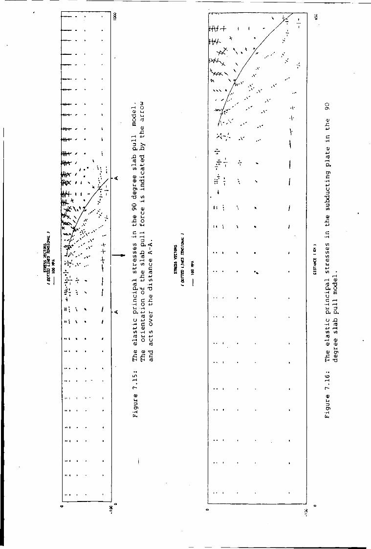
fc ~ a i
frf-» • - / i
I
•<
. 3 r H O <1J u V u 0 (T) e
0> r :
r H 4-1
3 >i a. xi XJ (TJ CD
r H 4 J 1/1
u 01 H <U T3 u C c n • H 01
T3 i n
O <J> CD
U <D U x : O
<4-4
c f—i • H »—( • in a < 01 1 1/1 X)
(Tl
ai r H 0) in U
• U c in m £ 4 J
r H 4-1 1/1
« J • H
• H 0 u 01 c c JC
• H o 4 J 1-1 • H
a, 4-> 03 01
u 4 J > • H c 0 4-1 cu in • •H in
ra U 4 J
i - t o u 01 nj
01 0) T 3 x : C
H
01 1-1 3
8 *
I -8 I
11
8
o ON
at
c •rH 0)
4-J
(0 r H
a c n c
u 3
3 3 1/1
0>
in 01 t/1 i/l 01 u
r - l 01 V
Cu o e
u C r H
• H r H l-i 3 CU CU U XI
• H (XJ 4 J r H
in i/i r H 01 01 01
U cu c n JZ 0) H T3
01 t-4 3 Cn
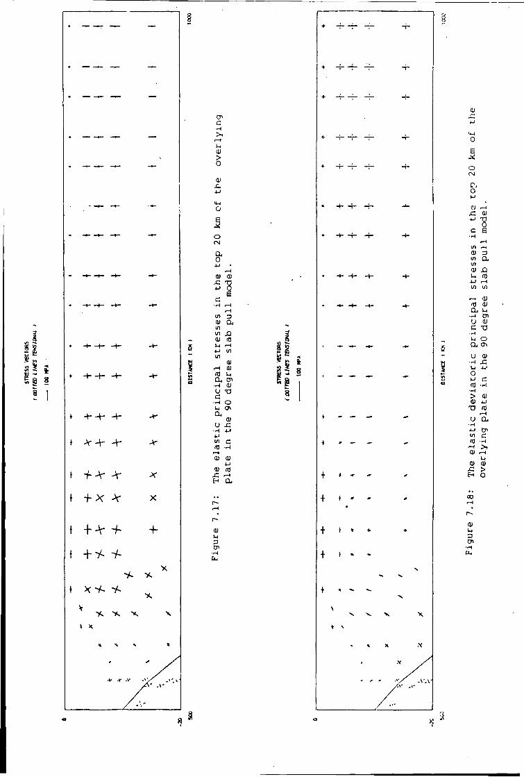
1
• •+-
t - f -X -V x
Vs x
» * N
+ .V -V .»
CP c
1-1 0) > o
01
e
o (N a o
01 01
u "8
IN 3 oi a IN J 3 oi m U r H 4-i in w
01 f - H 01 ro u
• H 01 U T 3 C o IN (JL a 01 U £
10 H r-i 01 01
4-1 o> m
x : - t H a,
0)
Cn • •H
2 ? 8
+ » -
+ • •
+ • *
>. v
-v-.\
0) sz 4-1
0
e
o
c, o 4-1 w r H
x : 01 4-J "8 c £
• H r H
L/> r-H
01 3 IN a IN 0i X I u m 4-1 r H M IN
r H ai IT) 0i a, u H Cn U 0) c TJ
•l-t u O a, a\
u 0) • H x : u 4 J
O 4-1 c: 03 •--!
•H
> 01 0> 4-1 X) m
r H
U a, • H 4-1 o» IN c nj - H
r H > 1 01 r H
1H 01 01
x : > H o
* 3
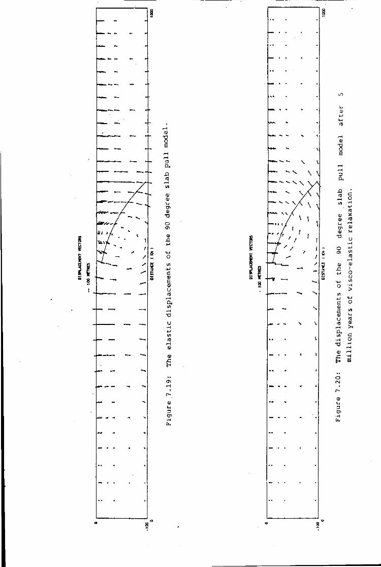
§
LTl
0)
-8 0)
•8 s
^ \ 1/1
01 ^ v \ 01
0)
ID nj
01 CP
T3 U
«3 s
s 1/1
in 3 as in
in cu N i/l
T3 0) <0
a. i/i ui (0
0 )
8 8
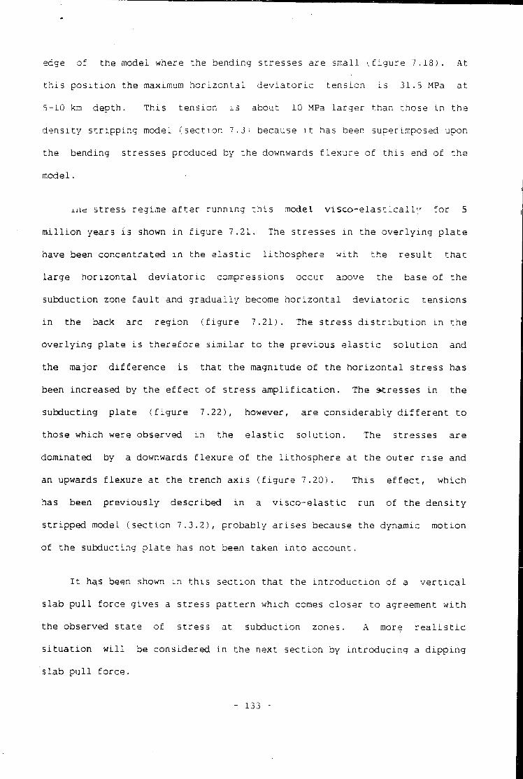
edge o f t h e model where t h e b e n d i n g s t r e s s e s a r e s m a l l ( f i g u r e 7 . 1 8 ) . At
t h i s p o s i t i o n t h e maximum h o r i z o n t a l d e v i a t o r i c t e n s i o n i s 31 .5 MPa a t
5-10 km d e p t h . T h i s t e n s i o n i s about 10 MPa l a r g e r t h a n t h o s e i n t h e
d e n s i t y s t r i p p i n g model ( s e c t i o n 7.3') because i t has been superimposed upon
t h e b e n d i n g s t r e s s e s produced by t h e downwards f l e x u r e o f t h i s end o f t h e
model.
iiirt s t r e s s r e g i m e a f t e r r u n n i n g t h i s model v i s c o - e l a s t i c a i l y f o r 5
m i l l i o n y e a r s i s shown i n f i g u r e 7 . 2 1 . The s t r e s s e s i n t h e o v e r l y i n g p l a t e
have been c o n c e n t r a t e d i n t h e e l a s t i c l i t h o s p h e r e w i t h t h e r e s u l t t h a t
l a r g e h o r i z o n t a l d e v i a t o r i c compressions o c c u r above t h e base o f t h e
s u b d u c t i o n zone f a u l t and g r a d u a l l y become h o r i z o n t a l d e v i a t o r i c t e n s i o n s
i n t h e back a r c r e g i o n ( f i g u r e 7 . 2 1 ) . The s t r e s s d i s t r i b u t i o n i n t h e
o v e r l y i n g p l a t e i s t h e r e f o r e s i m i l a r t o t h e p r e v i o u s e l a s t i c s o l u t i o n and
t h e major d i f f e r e n c e i s t h a t t h e magnitude o f t h e h o r i z o n t a l s t r e s s has
been i n c r e a s e d by t h e e f f e c t o f s t r e s s a m p l i f i c a t i o n . The P r e s s e s i n t h e
s u b d u c t i n g p l a t e ( f i g u r e 7 . 2 2 ) , however, a r e c o n s i d e r a b l y d i f f e r e n t t o
t h o s e w h i c h were o b s e r v e d i n t h e e l a s t i c s o l u t i o n . The s t r e s s e s a r e
do m i n a t e d by a downwards f l e x u r e o f t h e l i t h o s p h e r e a t t h e o u t e r r i s e and
an upwards f l e x u r e a t t h e t r e n c h a x i s ( f i g u r e 7 . 2 0 ) . T h i s e f f e c t , w h i c h
has been p r e v i o u s l y d e s c r i b e d i n a v i s c o - e l a s t i c r u n o f t h e d e n s i t y
s t r i p p e d model ( s e c t i o n 7 . 3 . 2 ) , p r o b a b l y a r i s e s because t h e dynamic m o t i o n
o f t h e s u b d u c t i n g p l a t e has n o t been t a k e n i n t o a c c o u n t .
I t has been shown i n t h i s s e c t i o n t h a t t h e i n t r o d u c t i o n o f a v e r t i c a l
s l a b p u l l f o r c e g i v e s a s t r e s s p a t t e r n which comes c l o s e r t o agreement w i t h
t h e o b served s t a t e o f s t r e s s a t s u b d u c t i o n zones. A more r e a l i s t i c
s i t u a t i o n w i l l be c o n s i d e r e d i n t h e ne x t s e c t i o n by i n t r o d u c i n g a d i p p i n g
s l a b p u l l f o r c e .
- 133 -
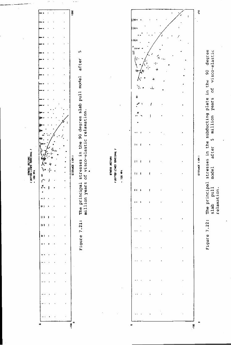
I
i s
II I >
I I I I
I I I I
I I I I
r - l <D
• c 0 e
i -H i - (
a ,
X I m •-I •
C o
0) • r H
ai 4-1 u rrj r j i X <u (0
i—i
(V o r- l
Ox u
m • r - l
r : 4-1 4-1 l / l
IT) c r - l
• r H 0) 1/1
1 0 0) u
</> U l i / l • rH
0) > • 1-1 4-1 M-J l / l o
r - l i n (0 1-4 a . m
• H
U > 4
d • r - | c I-I o a , • H
r -H ai r - 1
. c • r - |
H E
<N r -
a> u Z3
n
f ' '
I I I I
I I I I
i l l I
M I i
01 U <u •r-| 1-1 4-> Cn l/l <D rd T3 r - 4
01 O
1 O
rj> u i n • r H
V > r C 4 J
c ; 0
ni i/i 4-1 u m m
r - l a) a , > i
CP c c
• H o 4-1 •>H
u r - l
3 r - l
• H
J5 r j
6
l / l t n
01 . C 4-1 r- l
<U c 4 J
• rH <t- l
ro l / l ai in i/i r—1
0) 0) U | V 4-1 0 U l e
r -H
a r -H • •r-1 r—1 c u 3 o c a • r - |
• H 4-1 IH ra a , X
X I m m n) r -H
, C r -H <D H l / l M
CM CM
oi 1H 3 c j i
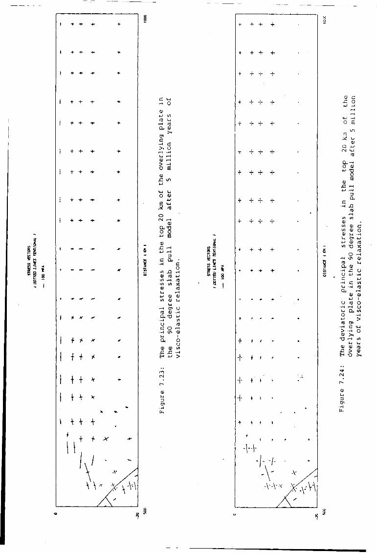
t + -t- *
+ • - t - - + •
+ + •+•
+ •+• -4-
\ i + *
I I f "
I T + *
c t-i H o 0) 4-1 l/l (0 l-i
.—i rO C L 0) CP c
- I c o l - l U —< 0) r—4 > o e 0) x : i n
O 0 ) 4-> S <*-l .2 fO
o CN rH
0)
4 J E CU
x : r - » 4-1 f—4
a c a, c
o 4-1
m i/i l/l 1/1 0) i-i W 0) J) i/i a; u
^ CP u
a , xs +•> rH l / l
(TJ
U £ O H Cfi 4)
I o u
(D CD i/l x : x :
r n
0) 1-1 3 CP
• l-l
B s 8 ,
+ + +
+ + +
+ T -r +
+ 4- ~
+ + + +
• - t - +
t ' ' '
"I" + ' '
•I- + " • ' •
•I- + » <
+ * » i
•/•
•V
•\-Vv ^ v - \ \
CD C x : 0
• H r - l
r - t —(
O s i n
i - i CU
o i - J <4-!
rtJ
O. r-H
0 4)
e 4) x :
—{
a c •H X) (0
r H 1/1 l/l cu •
l/l CD c t/1 0) o cu l - i • H
u 0> 4 J 4-1 0) <TJ i / i XI X
(0 o •~i
>—( O l <V ro u a 41
x ; u u 4 J —t c 4-1
— 1 c 1/1 1-1 • rH (TJ
a r -H 41 a>
4-1 1 u ro o
• H i -H u 1 - ! Q, 1/1 O 4-1 > <o CP •H c >4-t
> — I o >1
TJ r-H 1/1 l-l u
cu ai (t) xz > 01
•o >1
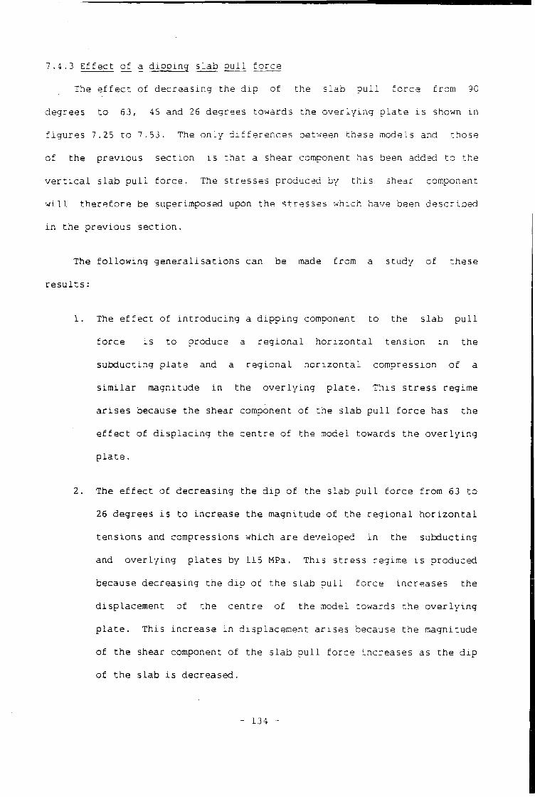
7.4.3 E f f e c t o f a d i p p i n g s l a b p u l l f o r c e
The e f f e c t o f d e c r e a s i n g t h e d i p o f t h e s l a b p u l l f o r c e f r o m 90
degrees t o 63, 45 and 26 degrees t o w a r d s t h e o v e r l y i n g p l a t e i s shown i n
f i g u r e s 7.25 t o 7.53. The o n l y d i f f e r e n c e s between t h e s e models and t h o s e
o f t h e p r e v i o u s s e c t i o n i s t h a t a shear component has been added t o t h e
v e r t i c a l s l a b p u l l f o r c e . The s t r e s s e s p r o d u c e d by t h i s shear component
w i l l t h e r e f o r e be superimposed upon t h e s t r e s s e s which have been d e s c r i b e d
i n t h e p r e v i o u s s e c t i o n .
The f o l l o w i n g g e n e r a l i s a t i o n s can be made fr o m a s t u d y o f t h e s e
r e s u l t s :
1. The e f f e c t o f i n t r o d u c i n g a d i p p i n g component t o t h e s l a b p u l l
f o r c e i s t o produce a r e g i o n a l h o r i z o n t a l t e n s i o n i n t h e
s u b d u c t i n g p l a t e and a r e g i o n a l h o r i z o n t a l c o m p r e s s i o n o f a
s i m i l a r magnitude i n t h e o v e r l y i n g p l a t e . T h i s s t r e s s regime
a r i s e s because t h e shear component o f t h e s l a b p u l l f o r c e has t h e
e f f e c t o f d i s p l a c i n g t h e c e n t r e o f t h e model towards t h e o v e r l y i n g
p l a t e .
2 . The e f f e c t o f d e c r e a s i n g t h e d i p o f t h e s l a b p u l l f o r c e f r o m 63 t o
26 degrees i s t o i n c r e a s e t h e m a g n i t u d e o f t h e r e g i o n a l h o r i z o n t a l
t e n s i o n s and compressions w h i c h a r e d e v e l o p e d i n t h e s u b d u c t i n g
and o v e r l y i n g p l a t e s by L15 MPa. T h i s s t r e s s regime i s p r o d u c e d
because d e c r e a s i n g t h e d i p o f t h e s i a b p u l l f o r c e i n c r e a s e s t h e
d i s p l a c e m e n t of t h e c e n t r e o f t h e model towards t h e o v e r l y i n g
p l a t e . T h i s i n c r e a s e i n d i s p l a c e m e n t a r i s e s because t h e m a g n i t u d e
o f t h e shear component o f t h e s l a b p u l l f o r c e i n c r e a s e s as t h e d i p
o f t h e s l a b i s d e c r e a s e d .
- 134 -
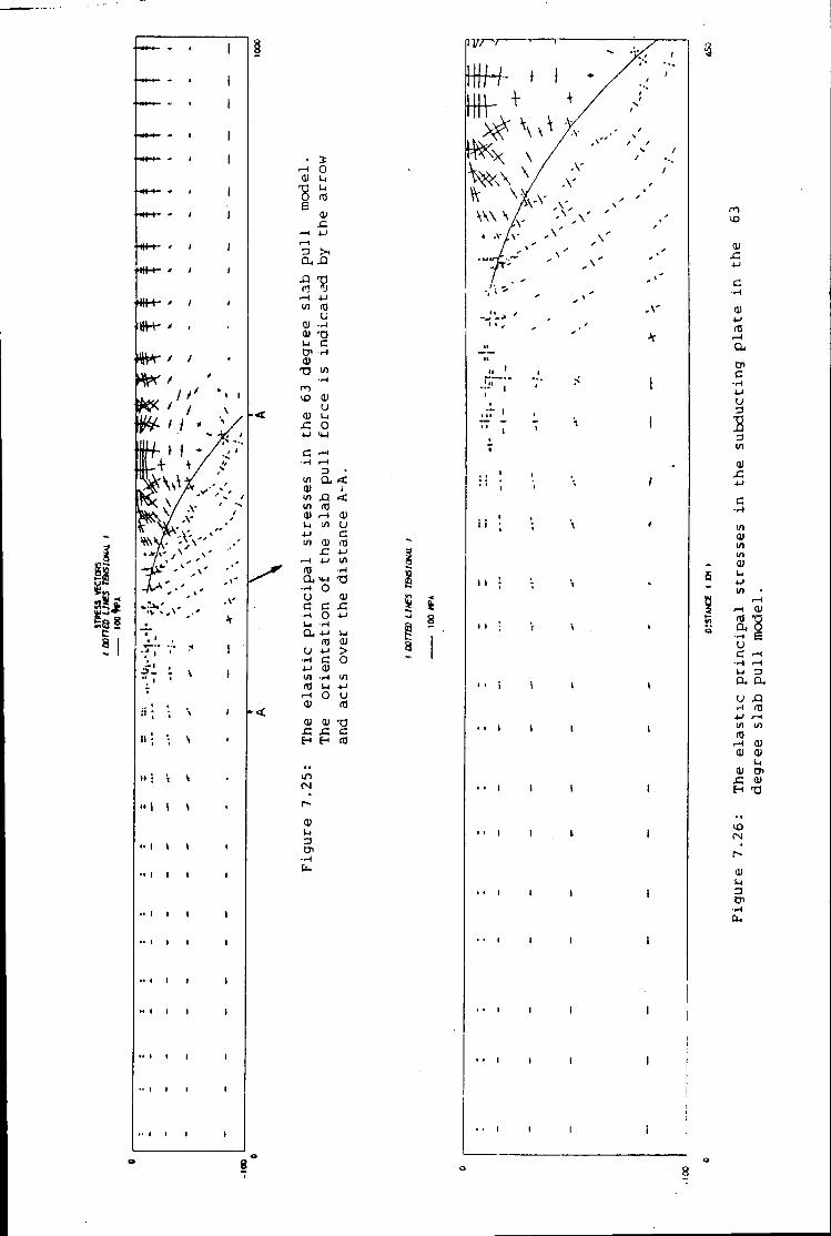
» i »
• 2 r H 0
1-1 u
0 m e at r H 4-J i—1 a > i a, XI XI "P a 1)
r H 4-1 in m u 0J •iH 0) X) Ul c cn - H
d) TD Ul
• H r o
a> u
a) u x: o
<4-l
c r H —t r H
3 • Ul a < a) I
XI < ui ai r H 01 Ul Ul u 4-1 c Ul 0) m 4->
r H 4-> U) • H
CU H-i T3 • H o u a) c c x:
• H o 4J 1-1 a, 4-i Ul
(0 u 4-1 > H c o 4-1 ai Ul • H Ul « Ui 4 J
r H O u 0) ro ai CD T3 c XI C
H
i n (N
u
• s
3
\ \ \ V
. V
s
x: 4J
<u 4 J (0 1—1 a< Oi c •H 4J
u 3
2 3 Ul a) x:
c •H m a> Ul Ul 0) 1-1
r H 0) m -a a, 0 •H e u CI r H
• H r H U 3 a. a , u XI
• H fO 4-1 r H Ul l / l
ro r H CD ai ai
u CD CP x: ai H T3
CN
0) u 3 t n
• • i i
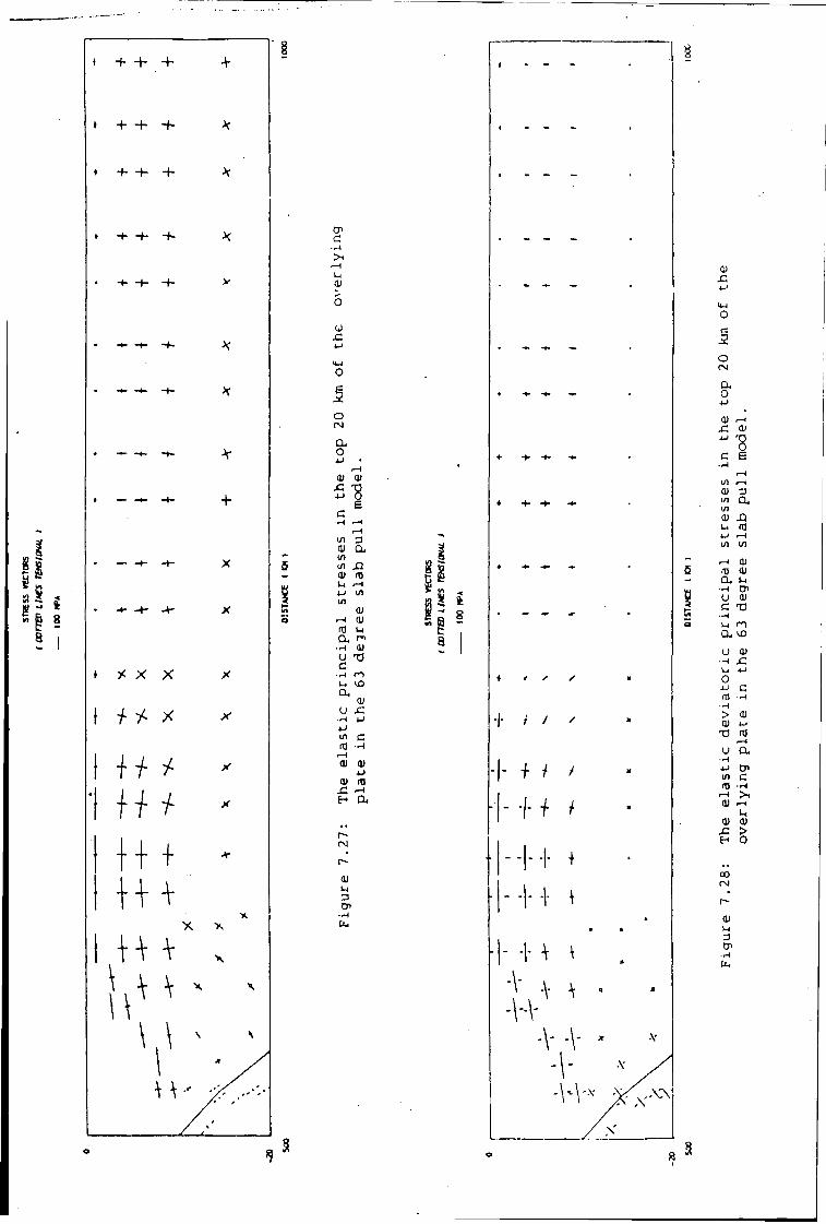
« + - + - + +
• -+• -+- -+• *
5 B
8 I
t * X X
I H /
1
H + H +
V
+
x x
CP C
—( > i
.—4 Ul
o (J
O
km
o
a o i->
.—i 01 01
5 " 8 e c —< •-<
in O o> a, — in
s in X ) 01 (0
UJ U r-H 4-1 1/1
5 1^ E> OJ a r-l 01
a ^ u -a c
a u £
•*-4 U u in C id w r-t QJ 0)
o) m H a
I N
r -
Ol u
8 s
B 8
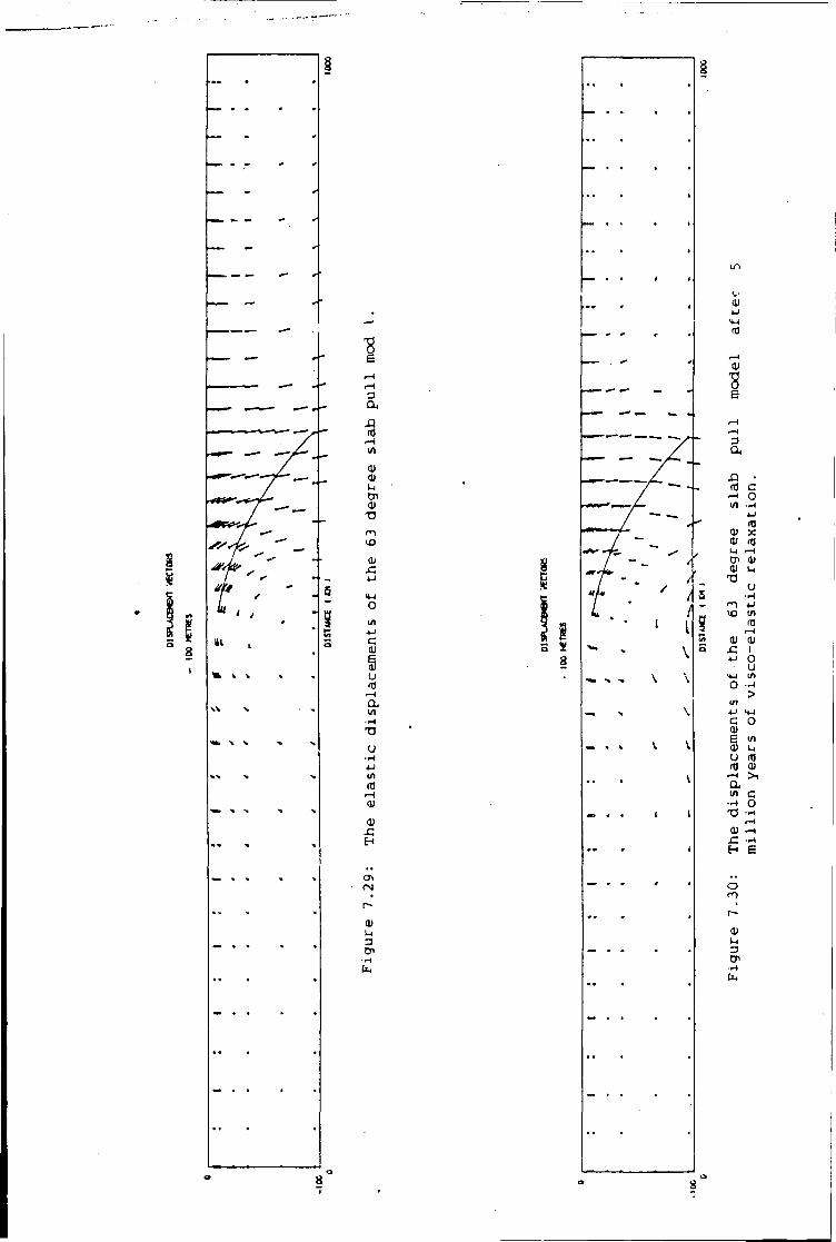
a
a QU
(0
oi ai u o> ai -a
m
01
c 01
u
a I / I
T3
U
0)
01 u 3
XI . (0 c l-( 0 to •A
i-> 0) 01 m i-i a> 0> 01 U
T3 u 4-1
VO ui
01 0) 1
4-1 o u
o —1 > 1/1 4-1 <4-4
C o 0) 6 1/1 01 u rtj
01 r-H >1 a VI c •H 0 -a •w
r-( 01 f-l c
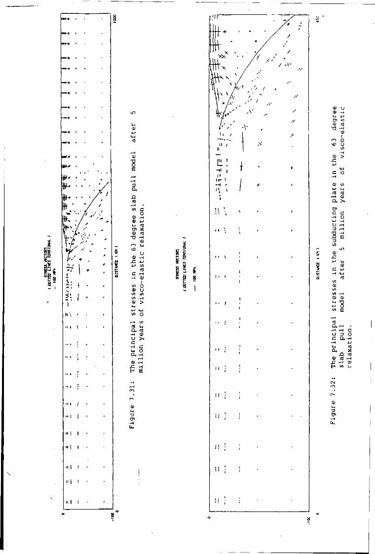
? • 1
•I i i \
i» \ '
"1 ;
•• I !
» I I
0)
<4-l
0J
e
3
a « r H
i/i c o
01 -H 0) ±J 1-1 ft) a) m
TJ - I 0>
c i u l£>
u 0) --H
-c - u 4-J in
(fl C rH
•H 01 I
i/i o QJ U ui 1/1 in H oi > u i/i O
r-l 1/1 OJ U a, in H CD U > c i-i o
r H OJ r H
H S
r -
0)
3 CP
8 i ! § 8 I
s
0) U •rl
lH 4-1 l/l
0) •a r H
01
m f o u 1/1
> c t H
c o
ai 1/1 u HJ
r H 01 a. >i t n c C
•rH o 4-1 -H U r H 3 r H
-r-l i5 —j
G i/i
i n 01
_c 4-1 u
0) c 4-) •H <4H
1/1 01 in i/i r H 01 01 u 4-1 0 l/l E
r H f0 Q j r H •
•rt r H c U 3 o c a •rH •H 4." lH m a , X
XI fO 0) m r H x: r H (!)
t/1 l.(
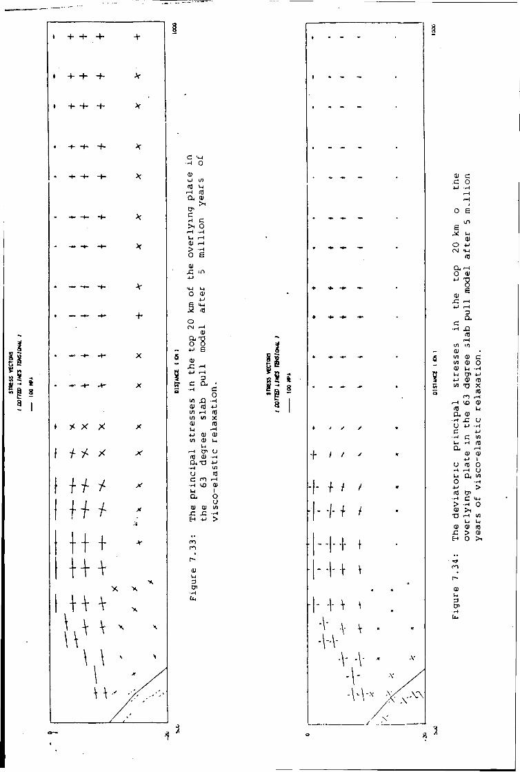
» + •+-
• + -+ - - * -
• H (-
t y. x x
f *
f i + /
H + H +
V
+
X x
8
•H 0 01 O 1/1 (0 U
i-i (0 a a) CP c
•H C > 0
rH -J . U rH
> o s ai 4-i
O 0) 4-1
o at
4-> E o> 4-1 r-l
3 c a . •
•H (3 0
in .Q •M 0) a) *J in r-H HJ i/i i/i 01 aj U4 r-l 4-1 01 01 1/1 0) U
r-4 cn u HJ 01 •H CU TD +J
(/l u IT) C rn rH
•-4 VO 0> u 1
o u
a) ai i/i •r-|
H 4J >
01 U 3 Di
•H Cl,
8 i
• / /• /
\ \ / '
I- + >
I - + i
• i - +
9
- -
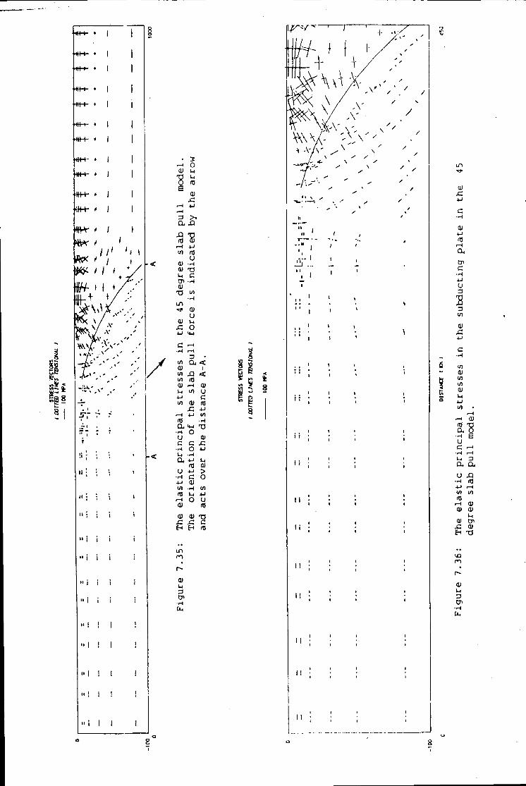
II I
" I I I
" i i i
" i i i
» I i i
•• ! ! i
" I ! I
" I I I
» ! I !
. 3: t—1 O 0) u
od
u rtJ
e 0)
r-1 4-» r-H 3 >< a xa XI ? m 4)
r - t +J i/i m
u 01 a) i-i c tn 01
T3 l/ l •-J.
ur> ^ > 0>
u 01 1-1
C o 4-> U-l
c • H r—1
3 • 1/1 a < 01 i l/> XI < Ul a) 01 0) u in u 4-> c 1/1 0) (0
x: 4-1 «—1 4-1 t/1 (0 a U-l
• H O u 0) c c x;
•r-l o 4-1 u a. 4-J
01 u 4-1 >
c o 4-1 01 t / i l/ l (0 l-l 4-1 .-t o u 0> m
01 01 T3 sz x: c H H
i n
ai L4 3
*. 8
I ii
T • ; • « .:. i
...
" L i
i
11
i i
i i
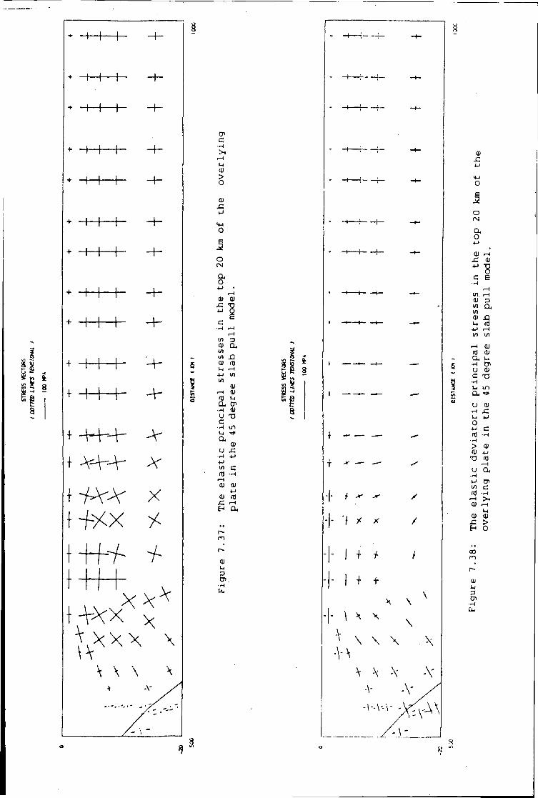
5
CP C
M 01 > o
CU x:
<4-l o
o (N
o
cu cu
a c
3 CU
X) rO
ui cu u i Ul CU u 4-1 Ul l/l
0) CD u CP 01
U TJ C
• H i n u •># a U XJ
(XJ a
c •rH
CU 0) 4-1
0) rfl X. rH en a ,
r o
01
3 CP.
I —
'\ * X /
\ - \ - - \ -
01 x : 4-J
•4-1 0
o
a o 4-1
01 rH c CU 4-1 •8 c I J
E •H rH
l/l rH CD 3 Ul a Ul CD X} u rd 4-J rH Ul Ul
rH 01 ra CD a 1-4
•H CP u 01 c T3
•H U i n
u cu •H SZ 1-1 4-1 o 4J c ro •H
•H > 0) 0) 4-J
T3 ro rH
U a •H 4J CP Ul c rd H
rH > 1 0) rH
H cu 01 c > H o
oo r o
r~
01 U 3 CP
•H U.
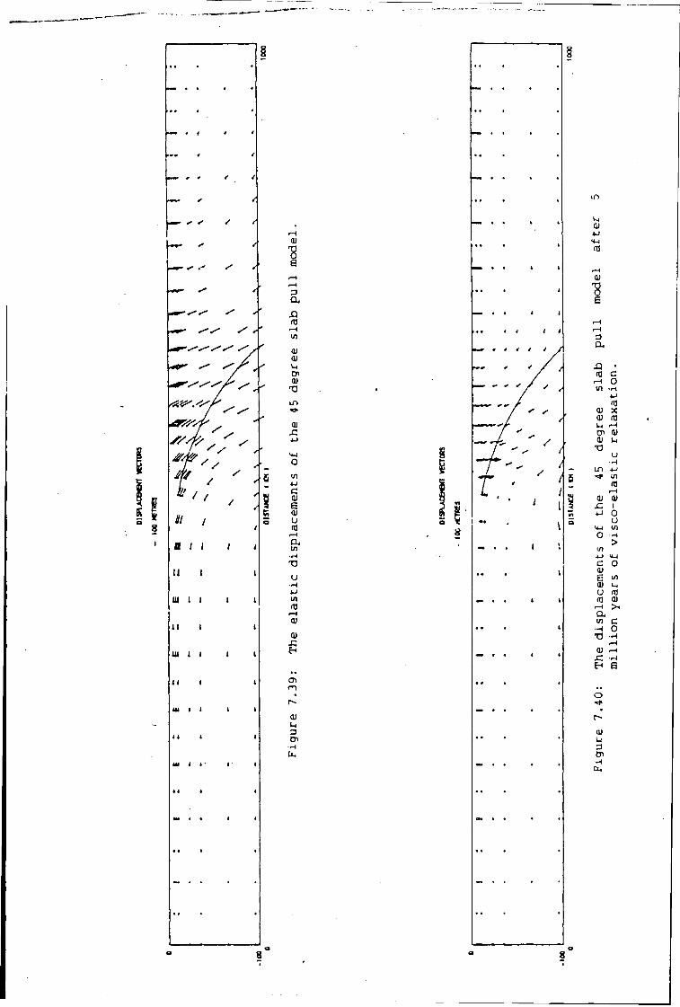
Ul t I
Ul I
01
"8 s
3 a XI
a) 0) In Cn 0)
TJ
01
<4H O
c 01 6 (U u m
r-l a. in
• H
T3
U
ITJ
01 x:
Ol <*1
01 u D
• H Ctv,
XI . m C rH o Ul •rH
4-> nj
01 >; 0) m in r-l 0> 01 01 u
XI u •r-l
LTl 4J I * l/l
m r—l ai i
4-1 0 u U-l in O
> i/l 4-> C O 01 E in 01 u u m m 01 r-l >< cu l/l c •-< o
T3 •H r-H
01 rH •rH s
8 8
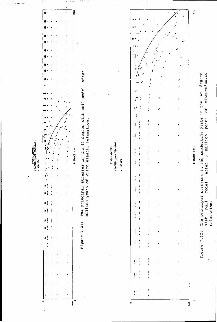
w • •
itH • •
iW • •
W« • •
I H - •
« • •
im - •
•
IW« •
IH • • • *..
I « 4 j « * •
— • • 1
r * •« * / /
"* . 'J
1 ' / «• •/ 1 •/•
• / / ./ / / * ***
/ /
* }•'» / ,•
1 / ; A '
/ *
- / < • /
i » ,
• • • *
/ , * ;
1 i t
M • ' 1
«i ! •
"i i •
•<• i
" I ;
»; i
«; i
ni
»;
"i
1 1 ;
i II ;
u 01 4-1
01
"8 e
3 a
X !
c o
(0 X
•—i 0 ) L4
01 01 u CP 01
T 3
i n
' u 01 —I
.C 4-1 4-< i/>
ITS C r-4
01 I o u I / I
•r-* >
IT) Q 4 —I U c
•H U a at c
01
3 CP
O
1/1 U l
(0 0 ) >i c o
I I
I I
I I
I I
I I
I I
I I
I I
0) CJ a U 4-» C " 1/1 0 ) m r-
0 )
0 u 01
01 > 4->
c O
01 1/1 4-> 1-1 (0 rt)
>—1 0 ) CL, > 1
CP c c
0 «-< •H u rH 3 1—1
•H XI e </i
i n
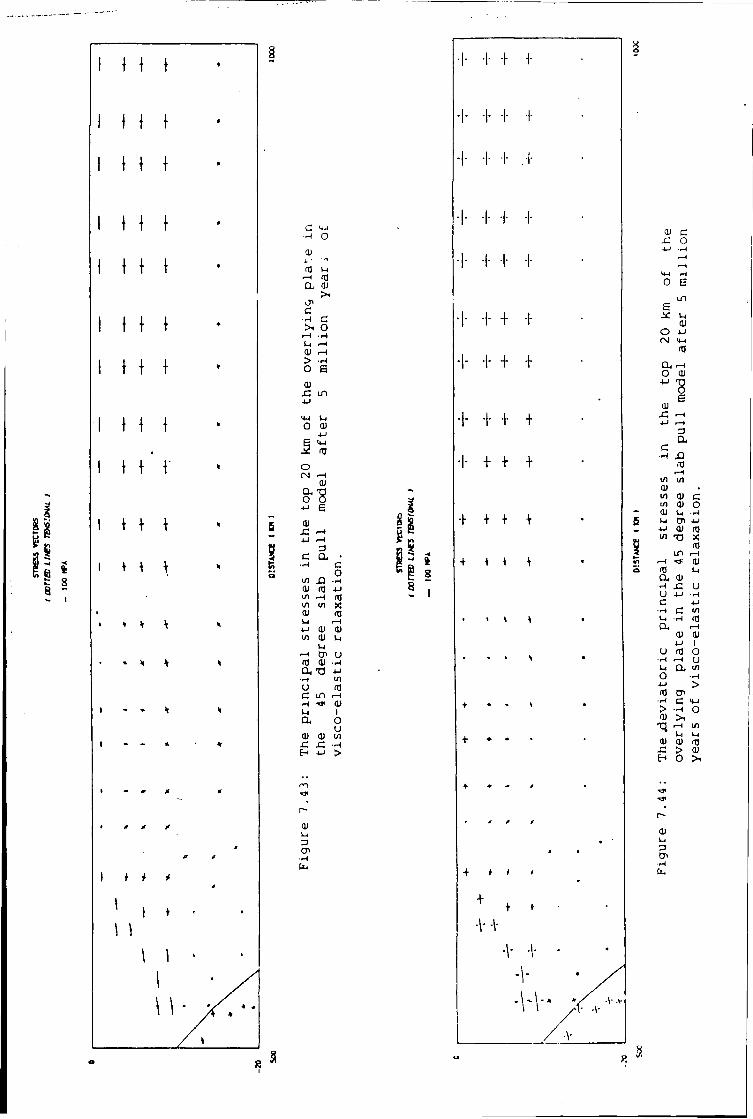
I t { } •
1 1 i } *
1 1 } } •
1 1 } } *
' 1 \ \ *
1 1 } \ •
' 1 \ \ *
•1 \ \ \
\' \
\ \
1 t 1 1 \ T
1 *
•I- I -I- +
1 I
\ i
c 14-4 • H O
0) 4 '
m i-l r H
a 01 > 1
c • H c
o r H • H 1-1 r H D r H
> • H O E 01 x: in u
14-1 1 4
o 01 4 J
E 14-1
ra O
r H 01
a. "3 0 0 4-1 E 01
JS r H 4 J r H
3 c CU •
• H c o
Ul X I • H 01 m 4-1 Ul r H (TJ Ul Ul X 01 m i - i r H 4-J ai 01 Ul 01 M
u r H CP U m 0) • H a, X J 4-1
• H Ul
u (0 c in r H
• H 01 L i 1 a o
u 01 01 U l
x: x: • H H 4 J >
01 1-1 3 CP
• H
-I- •!• -I-
•<
a * | 8 5 i
I- -I- + +
•I- + + +
•I- + + +
+ + + +
0 i
\ + •
•\- -\-
f> >—I
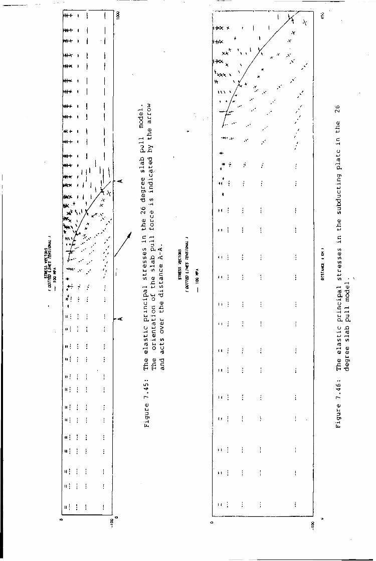
w - v t I t I
Ut t * • |
• I » I
UK* I | i
. 5 o
0) •O u 0 e
0) x:
r-l ~3 > i a, X5
"9 m $ * J
(«. u
0) 01 T3 u C CP 0) •o Ul
<N 0) U
01 u sz 0 4->
c r - l .—1 3
l / l O-. < 0) I
o> >-< 01 u </» u 4-1 C ui oi nj
£ 4 J i—I 4-* Ul IT) H a, <« •a •-4 O U O) c c c
• ~ i o a< 4-i i-i
HJ 0) 4-> > c o 01
u
U l
01
U l
01 0) T3 x: x: c H E-4 rtJ
i n
01
3 t n
a >
0) x: 4 J
c •r-i
U 4 J
a.
C - 4
4-1
du
e
X I 3 Ul
01 x; 4 J
c • H
Ul 0) Ul Ul a>
4-1 Ul •
H pH 0>
V cu 0
•r-t e u c • H r - l u 3 a. a u XI
• H m 4-J >—i Ul Ul
m r -4 0> 0) 01
u 0> cn x: 0)
T3
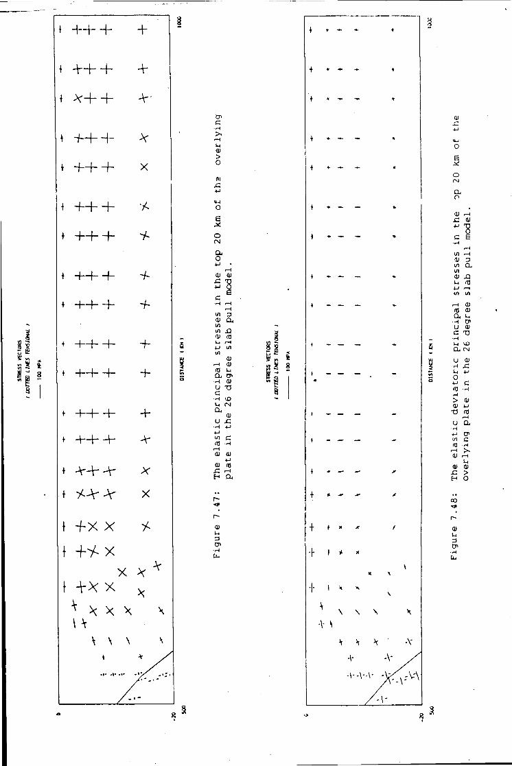
</i —» *• * s 8
++ +
-v-
x
- f -
+
+
X
} -f x x y-
x *
x x x
CP C
u 01
> o m
<*-l
o e o
CU o 01 01
2 a
ul 3 oi a , ui X ! 01 ra 1-4 r H 4-1 ui ui
0> r H 0) ra t i Cu en H 01 U TD c H lO u CM cu
0) U £
- H 4-1 4-1 "1 c ra H
r H 01 01
4-1 0) ro
X : r H H a
• 5 ?
01 u
CP • H U4
a * 8
+ • - »
+ « - > • -
4 - - -
•I- *
•I- » *
\ \ \
5
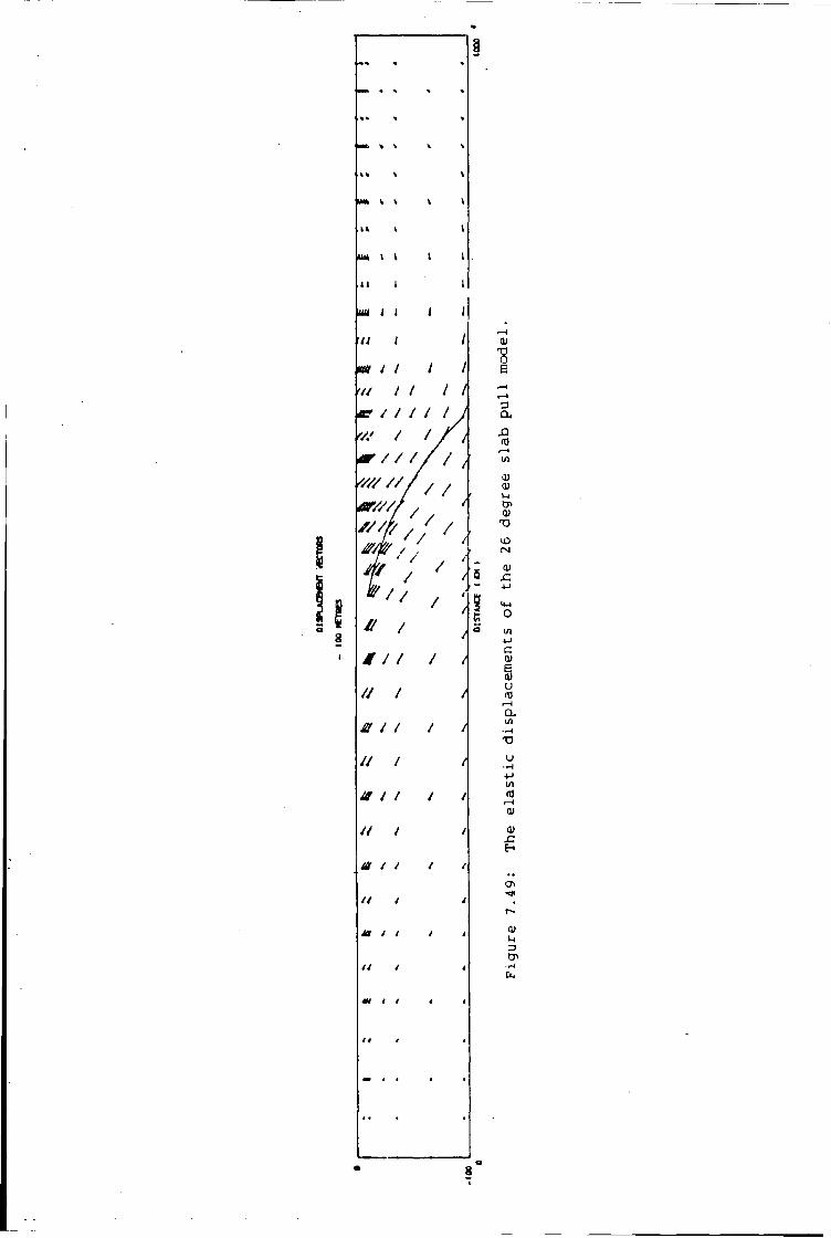
i
I t
m i
mil I I • a i t I t te / / / / / w / / or / / / / / j v// // / /
/ /
/ /
# /
t / /
// /
JB / /
// /
a / /
// /
ti i
a 8 "7
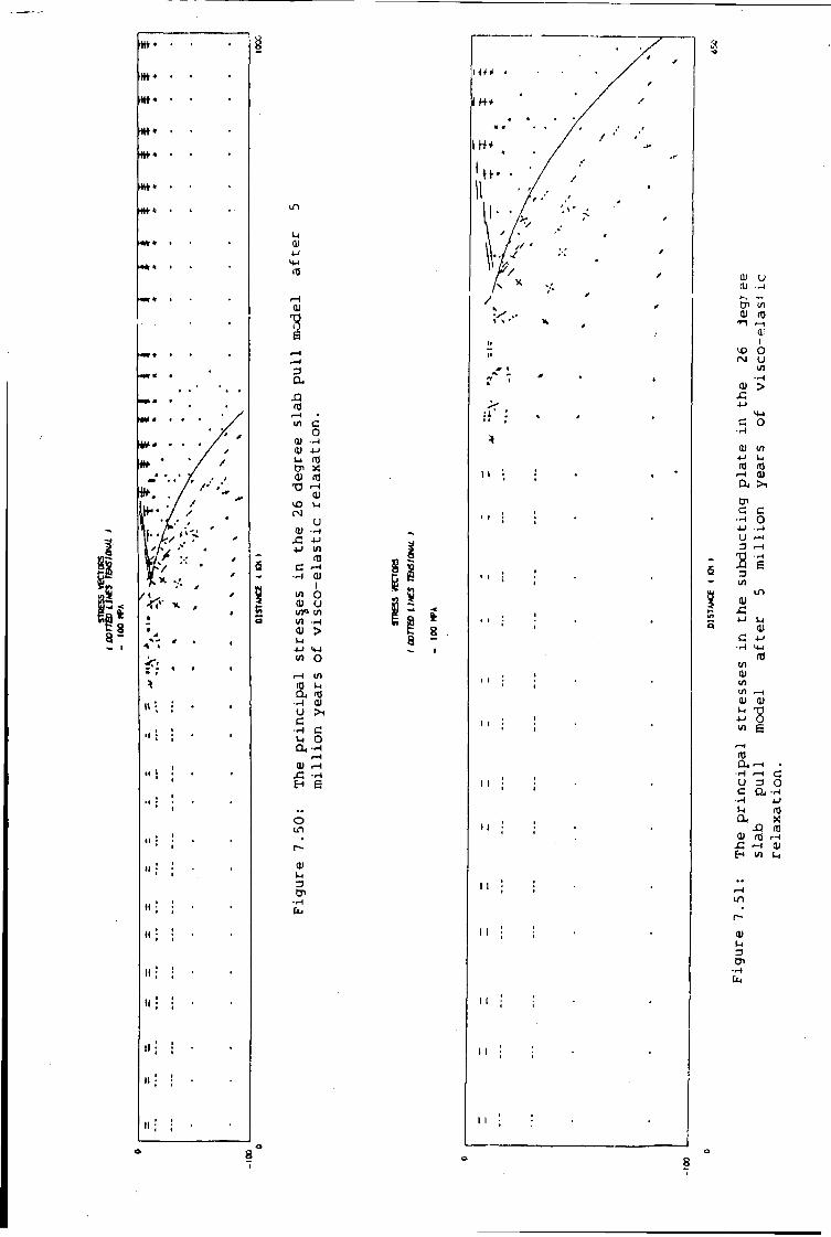
• •
• •
• •
• •
• • •
• • • •
*» « •
«*» • •
*m * •
«•» •
* • •
M l
*¥ • • • •
* r » • /' ' /
' / /
^ '/'/•'
/ *
x • /
> * •
• 0
»
• * 1
Z ' * * 1
• •
1 1 " I • •
l« I • (
, 1
• •
1
i 1 I I ;
* I
i t I I *
1 i •
" ; ;' •
•
»; i •
•
«! i
»'; ;'
L i 0>
01
£
3 CU XX I f l
r H w c
O 01 - H 0) 4-1 u rd cn x o> nj
X> 0)
v£> t-i CN
U 01 —I .C 4 J
4-i in (0
C r H •W 0)
I in O 0) U in* m U1 - H 0) > u 4-1 <4-l
in o i—i in n) u Cu nj
• H 0) U >i c
- H C u O d i - H
r H 01 r H x: - H H e
o i n
Oi L l 3 CP
-«-l
s i
it' :
11
11
0) u 01 • H
^ ,_• CP in 0)
" - I '—1 a-
VO f
o IN u in •rH
OI > SZ •t-i c o
• H
01 <n 4-1 L i m <tj r-i 0) a. > 1
CP c c • H o 4-1 rH U r H 3 r - l
T3 • H
25 E in
in 01 r: 4-1 u 0) C 4-J
Uj 03
in 01 in in r H 0> 0) L i 13 4-1 0 in B
r H (0 CU r H
• H r H C u 3 o c a • H
• H 4J L i nj 0k
XJ (D 0) r H
JZ r H 01 H in L,
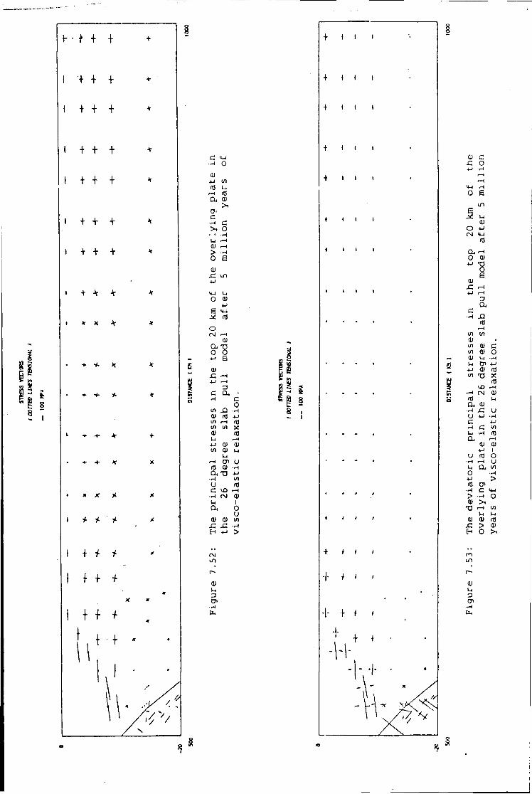
* + +
I + + +
I + + +
I + + +
I + + +
I + + +
i + + +
• + -V 4-
* x
~ + x
I t + +
c - H o Q) 4-1 rO u
r H ra a 01
> 1 0< C
• H c > ( o
r 1 —t u r H
1—1 > • H 0 6
0) sz LT1 4J
I j 0 01
4J e <*-i
rO
o .—i
01 a V 0 0 4-> E
0) jC . H
4-1 r H 3
c a H c
0 ui X I -4 0) m 4-1 i/i 1—1 m i/i Ul X 01 ro L i r H 4-1 01 01 t/1 01 U
1-1 i—I CP U rO Oi • H a TD 4-1
• H Ul u ra c
• H <s 01 U 1 a o
u 01 0) Ul
XI x: • H H 4-1 >
CN i n
0) L i 3 CP
- ft ^ 8 8 ~
+ t I i
+ 4 1 1
+ 1 1 1
4 ) 1 1
4 ) 1 1
• i > »
• i / /
+ 4 I I
"I" * > I
01 c x: o 4-1 H
r H r H
MH H 0 e
m u 01
o 4-1 (Nl H-l
rd
CU - H o 01 4-1 "8
E 01 c r H 4J r H
a c
• H X) rO
r H Ul U l 0) • Ul 0) c Ul 0) 0 01 L i • H u CP 4-> 4-1 01 ro Ul T f X
ro 1X1 r H
r H r-j 01 ra L l a 01
• H x: U u 4-1 • H c 4-1
• H c Ul • H m
a r H 01 CU
4-> 1 u rd o
• H r H u L| a Ul 0 • H 4-J > rd CP • H c <4-l
> • H o 01
T3 f—( Ul L l L i
01 01 rd x: > 0> H 0 ><
The d e f o r m a t i o n a f t e r a l l o w i n g t h e s e models t o r e l a x v i s c o - e l a s t i c a l l y
f o r 5 m i l l i o n y e a r s i s shown i n f i g u r e s 7.30 t o 7.34, 7.40 t o 7.44, and
7.50 t o 7.53. The e f f e c t o f t h i s v i s c o - e l a s t i c model i s t o c o n c e n t r a t e and
a m p l i f y t h e s t r e s s e s o b s e r v e d i n t h e e l a s t i c s o l u t i o n i n t o t h e e l a s t i c
l a y e r s o f t h e l i t h o s p h e r e .
7.4.4 D i s c u s s i o n
The models which have been p r e s e n t e d m t h i s s e c t i o n p r e d i c t t h a t zhe
e f f e c t o f t h e v e r t i c a l component o f t h e s l a b p u l l f o r c e i s t o i n d u c e
h o r i z o n t a l t e n s i o n i n t h e s u b d u c t i n g p l a t e and h o r i z o n t a l c o m p r e s s i o n i n
t h e o v e r y l i n g p l a t e between t h e t r e n c h a x i s and t h e v o l c a n i c a r c . T h i s
l a t e r a l v a r i a t i o n o f t h e h o r i z o n t a l s t r e s s i s o b s e r v e d a t a l l s u b d u c t i o n
zones. The models t h e r e f o r e suggest t h a t t h e s l a b p u l l f o r c e c o n t r i b u t e s
t o t h e o b s e r v e d l a t e r a l v a r i a t i o n o f s t r e s s a c r o s s t h e s t r i k e o f s u b d u c t i o n
zones.
The models show t h a t a h o r i z o n t a l component o f s l a b p u l l f o r c e
produces a r e g i o n a l h o r i z o n t a l t e n s i o n i n t h e s u b d u c t i n g p l a t e and a
r e g i o n a l h o r i z o n t a l compression i n t h e o v e r l y i n g p l a t e . Because t h e s l a b
p u l l f o r c e p r o b a b l y a c t s a p p r o x i m a t e l y down t h e d i p o f t h e s u b d u c t i n g s l a b ,
i t may e x p l a i n t h e o b s e r v e d v a r i a t i o n i n t h e s t r e s s regime between t h e back
a r c areas o f d i f f e r e n t s u b d u c t i o n zones. The models p r e d i c t t h a t
s u b d u c t i o n zones w i t h a s h a l l o w d i p s h o u l d have co m p r e s s i o n i n t h e back a r c
areas w h i l s t t h o s e w i t h h i g h d i p s s h o u l d be l e s s c o m p r e s s i v e . T h i s
p r e d i c t i o n i s i n r e a s o n a b l e agreement w i t h o b s e r v a t i o n s .
- 1 3 5 -
7.4.5 L i m i t a t i o n s of the models
The models i n t h i s s e c t i o n have three main l i m i t a t i o n s .
F i r s t l y , , the magnitude of the v e r t i c a l component of the slab p u l l
f o r c e i s an upper l i m i t . This i s because i t has been estimated from a 5 km
deep trench which i s the l a r g e s t observed depth of any trench i.Greilet and
LubOxS, 1932). The magnitude of the stresses i n the medals are t h e r e f o r e
an upper l i m i t on those which the slab p u l l f o r c e produces. The models
t h e r e f o r e demonstrate the general i m p l i c a t i o n s of the slab p u l l f o r c e
rat h e r than make s p e c i f i c p r e d i c t i o n s f o r the magnitude of the stresses at
any p a r t i c u l a r subduction zone. The models imply, however, t h a t f o r a
lower slab p u l l f o r c e the magnitude of the stress would be reduced.
The second l i m i t a t i o n i s t h a t mantle drag, which r e s i s t s the motion of
the subducting p l a t e , has been neglected. I t i s , however, u n l i k e l y t h a t
t h i s f o r c e could have an important e f f e c t on the stress regime which has
been modelled. This i s because the r e s i s t a n c e produced by mantle drag over
the 500 km long base of the subducting p l a t e would be small.
The t h i r d l i m i t a t i o n i s t h a t the subduction zone f a u l t has been
assumed to be locked. Stresses i n these models have t h e r e f o r e been
t r a n s m i t t e d p e r f e c t l y across the f a u l t zone. This i s u n r e a l i s t i c because
i t neglects any e f f e c t of the e l a s t i c p r o p e r t i e s of the subduction zone
f a u l t . To overcome t h i s l i m i t a t i o n the e f f e c t of f r e e i n g the f a u l t i s
considered i n the next s e c t i o n .
7.5 E f f e c t Of The 5ubduction Zone Fault
The e f f e c t of l o c k i n g the subduction zone f a u l t i s to c o n s t r a i n each
dual node to have i d e n t i c a l displacements. The previous models have
- 136 -
consequently behaved as a s i n g l e e l a s t i c continuum i n which s t r e s s i s
t r a n s m i t t e d p e r f e c t l y across the f a u l t plane. They have t h e r e f o r e assumed
tha t the p l a t e s are p e r f e c t l y e l a s t i c a l l y coupled a t the subduction zone
f a u l t .
Kanamori (1977) suggested t h a t the coupling between the p l a t e s a r
sutduction zones i s s p a c i a i i y v a r i a b l e . He demonstrated t h a t the seismic
s l i p r a t e at subducticn ^.outs .vhich have great t h r u s t earthquakes (e.g.
C h i l e ) i s comparable w i t h the subduction r a t e p r e d i c t e d by p l a t e motion
models. Elsewhere, where there are no great t h r u s t earthquakes (e.g.
Marianas), the subduction r a t e i s many times greater than the seismic s l i p
r a t e . Kanamori explained t h i s observation by proposing t h a t the degree of
mechanical co u p l i n g of the p l a t e s v a r i e s between d i f f e r e n t subduction
zones. Kanamori, and more r e c e n t l y Uyeda and Kanamori (1979), also
demonstrated t h a t the subduction zones at which p l a t e s are s t r o n g l y coupled
have compression i n the back arc region w h i l s t those which are weakly
coupled have t e n s i o n a l stresses which give r i s e t o a c t i v e back arc
spreading.
These observations suggest t h a t the stress regime i n the o v e r l y i n g
p l a t e may be c o n t r o l l e d by the degree of mechanical c o u p l i n g between the
p l a t e s at a subduction zone. The aim of t h i s s e c t i o n i s t h e r e f o r e t o
i n v e s t i g a t e the e f f e c t of v a r y i n g the e l a s t i c p r o p e r t i e s of the subduction
zone f a u l t .
7.5.1 D e s c r i p t i o n of the f i n i t e element model
The e f f e c t of d i f f e r e n t p r o p e r t i e s of the subduction zone f a u l t has
been i n v e s t i g a t e d by reducing the shear s t i f f n e s s of the 45 degree slab
p u l l model ( s e c t i o n 7.4.2) to values of 1.0x10 N m , b.OxlO N m and
- 137 -
1.0x10% m~' The f a u l t was assumed to have a c o e f f i c i e n t of f r i c t i o n equal
to 0.1 and f r i c t i o n a l s l i d i n g was allowed to occur. To ensure t h a t both
sides of the f a u l t plane remain i n contact d u r i n g f r i c t i o n a l s l i d i n g the
normal s t i f f n e s s of the f a u l t has been assigned a value of L.Oxlo'SN nf.1
7.5.2 E f f e c t of reducing the shear s t i f f n e s s of the subduction zone f a u l t
The stress regime which has been c a l c u l a t e d a f t e r reducing the shear is _ i io -|
s t i f f n e s s of the subduction zone f a u l t from L.OxlO N m to 1.0x10 H m,
5.0x10% m'1 and 1.0x10% m"1 i s shown i n f i g u r e s 7.35 t o 7.39, 7.54 t o
7.57, 7.58 t o 7.61 and 7.62 to 7.65 r e s p e c t i v e l y . The v a r i a t i o n of the
h o r i z o n t a l d e v i a t o r i c stress w i t h depth at the r i g h t hand edge of the
o v e r l y i n g p l a t e and the l e f t hand edge of the subducting p l a t e i s shown i n
f i g u r e s 7.66 and 7.67.
These r e s u l t s demonstrate t h a t reducing the shear s t i f f n e s s of the i5 -i i - i subduction zone f a u l t from 1.0x10 N m to 1.0x10 N m has two e f f e c t s upon
the r e g i o n a l stress regime which i s produced by the H o r i z o n t a l component of
the slab p u l l f o r c e . F i r s t l y , i t reduces the r e g i o n a l h o r i z o n t a l
compression i n the o v e r l y i n g p l a t e by 40 MPa i n the mantle and 17.5 MPa i n
the c r u s t (the d i f f e r e n c e being due to the c o n t r a s t i n g Young's moduli of
these l a y e r s ) . The magnitude of the r e g i o n a l h o r i z o n t a l compression which
i s t r a n s m i t t e d i n t o the o v e r l y i n g p l a t e by the h o r i z o n t a l component of the
slab p u l l f o r c e i s t h e r e f o r e s t r o n g l y c o n t r o l l e d by the shear s t i f f n e s s of
the subduction zone f a u l t . Secondly, the r e g i o n a l h o r i z o n t a l tension i n
the subducting p l a t e i s increased by a commeasurate amount. The e f f e c t of
reducing the shear s t i f f n e s s of the subduction zone f a u l t i s t h e r e f o r e t o
make the h o r i z o n t a l stresses more t e n s i o n a l throughout the model.
- 138 -
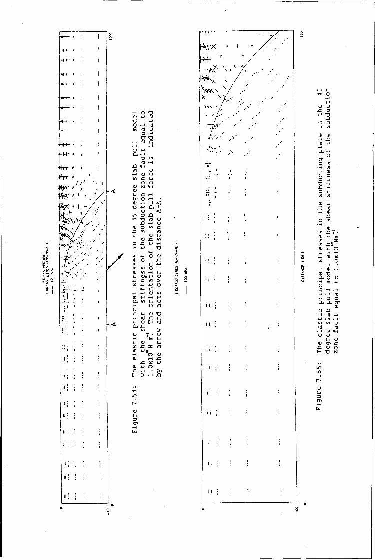
-<
0 "9 0) 4-> CD
4-1 0 r—i r0 E ra U
^ a 1 T3 —4 0) C i—1 • r 4 3 4 J
a 1/1
m XI <*-( ra oi
a) u i/i c u o o (V N 0) u C r—i
0 1 o i - | • 0) • r - | a < T> 4-J a 1
u < 3 XI
(0 0 )
25 < u 01 3 in c
U l ra 4-1 ai 4 J
01 in c XI 4-1 • H
• H 4 J X) 1/1 O 0) 0) o JS 1/1 c 4-1 W 1/1 o 0) W • H u u 0> 4-1 c ra > U1 4-< 0
>4-l c r H —( oi in (tl 4 J • r - | 4-1
a l/l u • H o ra u c u a> n
• H fO x: c U 0) H ra a, £
1/1
u r * o 6 l-l
4 J 0) u U l £ 2 ra m
O a> at i—t G
Xt X 4->
at 4-1 o • H • > i
H i H XI
in
tl) i-i 3 CP
8 i
in c r j> 0
-l 4-1
0) u X a 4-> 3 C 3
• H in 0) 0)
4-1 J C ID 4-> I
o CP c in
•l-l in 4-> ai u c 3 U J
2 • H 3 4-)
l/l in u
x: ra 4-> ai
x: c in
• H 0)
l/l X 7 * a> 4 J E i/i Z i/i x s 0) 4-1 O u • H i - ( 4-1 2 X in O
l - l • r—l at (0 *n a. Q O
• H £ 4-1
u c 1—I i - 4
l - l ra U 3 3 a, • 4 tr
o> u X!
•<H ra 4-> 4-1 i-H
in in 3 ra rfl .-i 01 14-1 0) 0)
l-i 01 ai CP c
01 0 TJ N
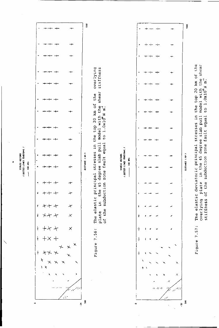
I s l a § a
* •+--+- -+•
\ x
t + X + x
\ \ \
CP ui C ui
• H 0) >i c >-) <l-l 0) - H > 4-1 0 ui
01 (0 . C 0)
•u .c l/l
O (P7 • £ e
6 * J Z
£ o O 4 J t 5 < N W r - i a, o o • 4-1 0) r - l
0) "8 O JC B 4-i
• H D P a cr
tn o> ai xi U l f f l 4-1 l / l H r H 111 U l
1-1
3 (tj
4J 0) <*-J U l Q)
0) c o
a, x i N H U LD C • » H
a, J S
c o
u
•iJ 2 4-> C 3 l/l r l in m
r H 0 ) ai a) J C
4-1 4-1 C -> "4-1 H a O i£> in
o> I-I a CP
i s . s -in 9 fc a
0) 1-4 x: 4-J a)
U )
o a> 7 • e 4-'
o I N 4J o
• H r-l
a s X 0 o 4-1 ,—i •
s: 0 0 4-J 6 4-) c —1 .-1
• H r—1 (0 3 3
V I a, cr 01 01 U l XI U l ra 4-< 01 l-< r-4 l-i 1/1 3 4-1 <T3 U l 0)
a) r-H u 01
W> c a a) o
• H T 3 N u c LO c —1 o u a 0) 4.J
x: U u 4J 3
T2 1-1 c i5 o •r-4. 3 4J U l
m - H 0 ) ai > 4-> ai m 4J
XI r-l a, H-l
u o • H 4-1 CP U l U l U l
(tJ 01 • -H >. c 0) I-I <4-l
I-I >4-l 0) a> •r-i > 4J H o U l
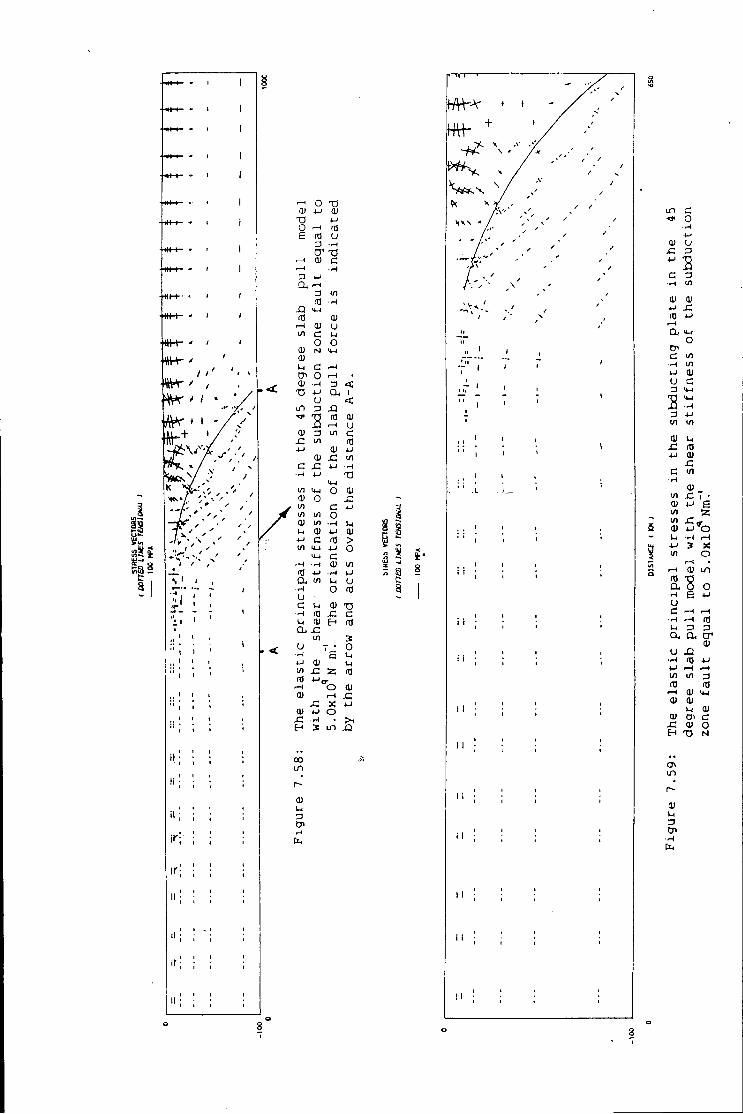
i i
i i
• i i
i t <
i i •
1—I o T3 0) 4-1 0)
TJ •u 0 r—\ m £ <n u
3 •w ,—i o> c i — i 1 3 4 J
3
ra H
a 0)
r-t 01 u m c u
o o o) N <4 - l 0) u, c en 0 r-H • 0J —1 3 < T3 4 -J a . 1
u < in 3 XI
01 xS .—t u
0) 3 i / i c xz i/) a) 4 -J 0) 4 J
QJ Ul c £ 4 -J •H
•r - l 4-> n l/l U - i O 01 0 XC l/l c 4 J 1/1 i / i o 0) i / i •H Ul 1-1 at 4 J 0) 4-J c m > in 14-1 4-1 0
14-4 c ~< •--1 0) i / i m 4 -J •H 4 J
in 1-1 u o <a
U c i-i 01
<a x: ai E-I
a , xz m
U 7 • •~i e 4 J 01 "1 X: 2 n) 4 - i „ .
•H O 01
JZ X 01 4-1 O x: H • >-,
00
c (0
3 0 tj I - I
m 01
x:
0) u a en
• H
t
T 1
i • ~ ' • i
i
i i
m c 0 . 4
0) u xz 3 4 J 2 c 3 •H Ul
0) 0> i-> xz IXJ 4-1 •—i
a U-l
o CP
c Ul Ul
4 J 01 U c 3
>4 - l
is —( 3 4 - J Ul Ul
01 xz m 4-1 01
x: c Ul
01 l/l xz i ' 01 u 6 Ul Z Ul XZ 0) 4 J o I-i •.-( rH 4 J X! Ul O
>-( • r—i 0)
"5 a 0 o •H E 4 J u d »—1
•rH H (0 1-1 3 3
a a cr o>
u X! 10 4-1
4-1 i - H r-4 Ul Ul 3 (TJ (TJ
. -H Oi <4 - l 01 Ol
l-i 01 01 Oi c
x: 01 0 T5 N
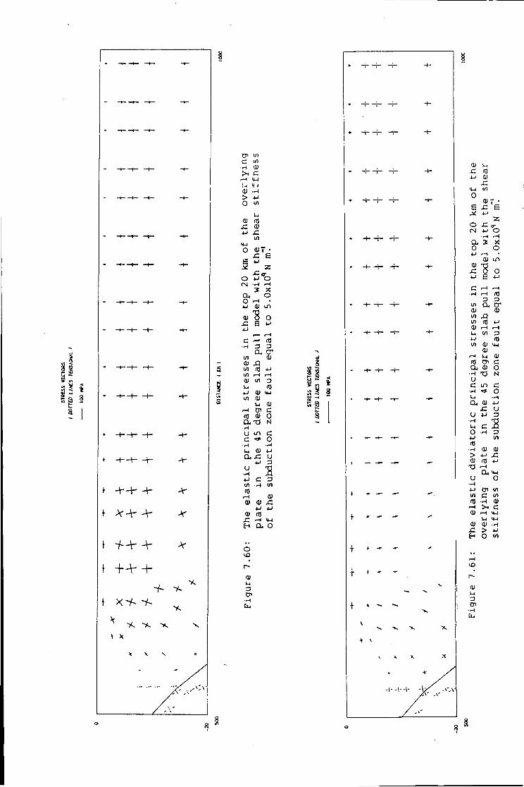
n
a -
a I
^ x
* \ \
CP w C in
• H 0) >i c r-1 M-l
1/1
u Q) «J
£ 0) 4 J £
in U-l O 0)7 • £ e
2 z XI <r O <-> O
(M -H rH a o 0 • 4-1 0) in
H I ? O x: e *J
• — ( i — ( c ^ rcJ
•H 3 3 a cr in d) ai X) w ni -u l/l H H 01 w 3 u m
4-< 0 ) <4-i in 0)
U 0 ) H 0 1 C m a> o a, T > N -1-4 u m c c o H —t M 11 ^
o< x: u 4 J 3
.y s 4- i C 3 1/1 H 1/1
m a) oi x:
4-1 4->
a) ra XT r-t <*-!
H a o o I D
0) u 3 cn •-(
% 8
Is I
• — ^
• I -
0)
4-> 0) x:
0 0) 1 * s x; 6
4 - ' 2
o x: <r 4 J O
rH a, X o o
4-" • 0) m
0) "5 x: 0 O 4 - J H 4-1
c r—1 r-H •rH r-1 m
3 3 1/1 a, tr 0) 0) l/l t/1 0) r-t u V 3
4 J nj t/1 0) <4-l
a) i—1 1-4 01 (0 c a. a> o •H T 3 N u c in c
• H o I j - H
a 0) 4->
x; u u 4-1 3
• H U c xl o •H 3 4-1 l/l <a
•r-| 0) 0)
> 4-1 x: ( t j 4-1
T 3
a <4-l U 0
• H 4-1 cn l/l l/l c in
01 f-l C D M-l
U K-l 0) 0) •H sz > 4-1
H o in
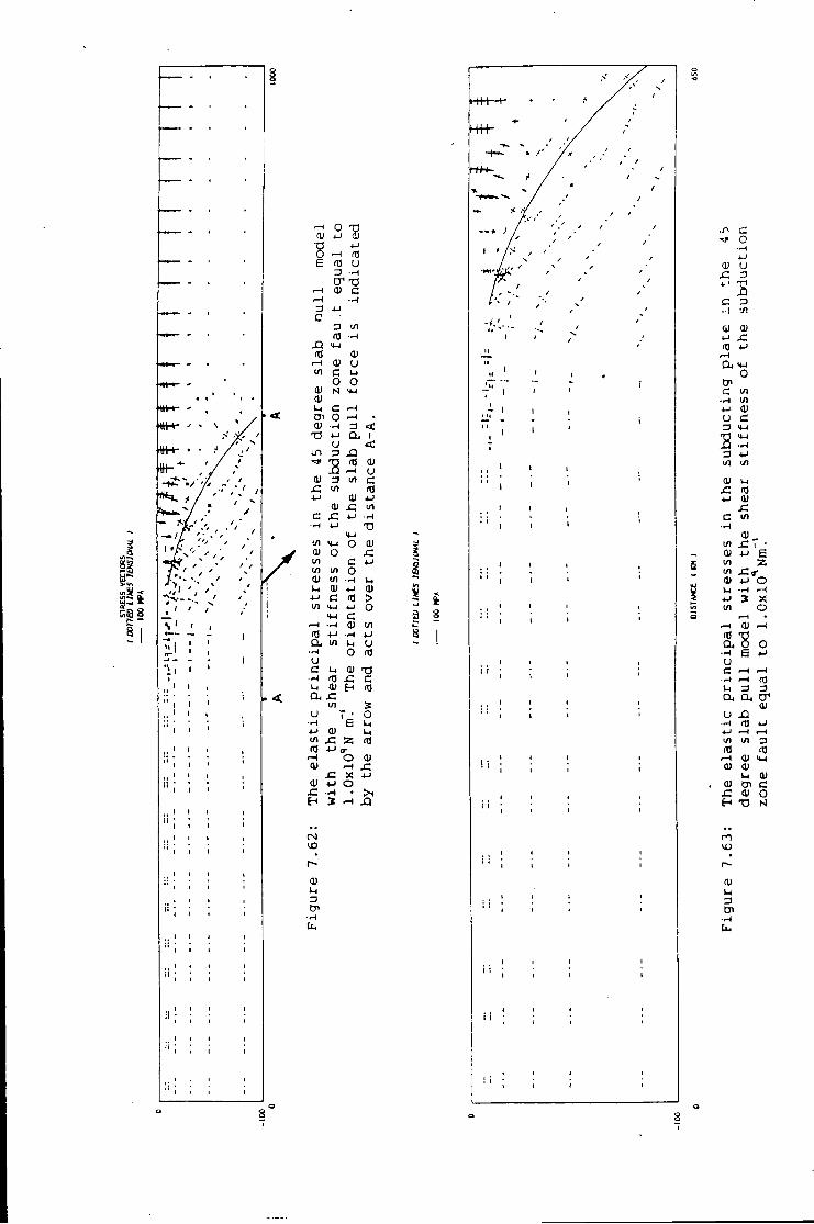
a i
1 1 O T3 (1) * J 4 X) j-i o H m e ra u ^ 0 ) c 3 4 J C
3 ra ra --I (D c o QJ N 01 U CP 0)
in
c o
L A
4-1
u 3 s
0) 3 X m 4 J
O) C X
• H 4-1
01 u u o
V I
3 -a:
Q, l
XI ra
0) u c ra 4-1 1/1
-<H
in vt O CU 0) O m in l/l 01 in U 01 -M C W vi
ra Q, l/l
X C 4-1
o 01 > O c
0) in
ra
u u o ra u c • H ra x u 0 ) H a x
in u V
4-> ai w .c 55 ra +J o-r-l O 01 0 ) rH
X X 4-1 0) 4-1 O X • >, H J H J 3
( N l£>
01 TJ " c ra o u u ra
0) i-i 3 CP
• H
i
T ' '
i l l 1
". 1 '
,, 1 1 >
'' i i
I I <
LTI c •O" o 01 u
X 3 4- 1 s c 3 .•! 7!
OJ 01 4-1 X ra 4-1 r-H CU vi
0 CP G in
•H m 4-1 0) U 3 fn
bd
if
3 4 J m in 01 i-i
X ra 4-1 0) X
c in
in X i • oi 4 J e in 2 in X « -01 4-1 O l-l r-l 4 J 3 X in o
i—i H HI r l ra v a. o o •-1 E 4-> u C i-l • i - i I - H ra l-i 3 3 a a D 1
01 U XX
• H ra 4-1 4-1 --I .—I in in 3 ra ra r-H 01 VI CU 0 )
I-i 01 01 CP c
X 01 o H T 3 N
lO
01 l-i 3 CP
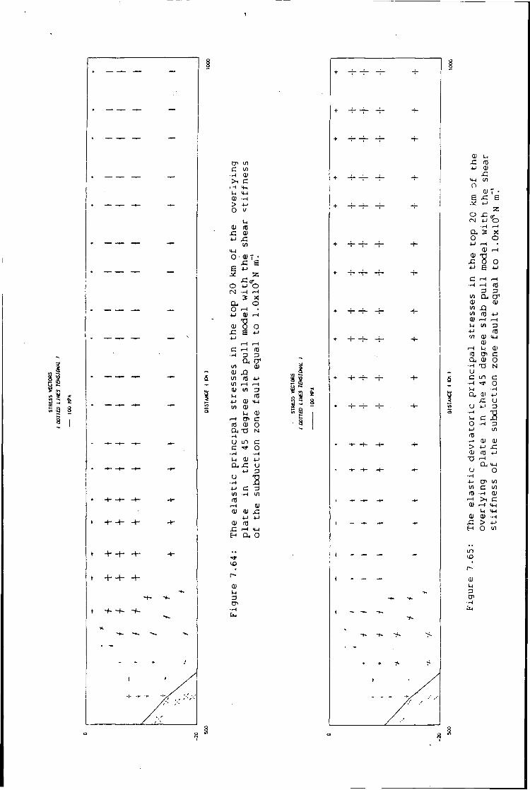
a i
tP Ul C u>
• H 0) >i c
. H I-I <4H 01 • H
> 4-i
o U
I - I oi 03
0) •u x:
U) <4-l 0 o> " •
x: e E 4-> y 2
X l a -O 4J o CM •r-l r - l
s X a, o 0 r H • 4-1 0> r H
OJ "8 O x: E 4 J 4 J
r H r H c r H rtj
• H a 3 a CP
U l 01 a> r Q in IT) 4-1 Ul r H r H
Ul 3 >-i m 4-> 01 u-l l / l 01
l-i 0) r - l CP c m 0> o a -a N H u in c c o
• H H U 0> 4J a x: u
4-1 3 u
• H - Q 4-J C 3 l / l • H Ul (TJ
r - l 0) 0 ) <u x:
4-1 4-1 cu m x: r H «H H o
Id r~ 0) u 3 CP
ii » a % § 3 8 In § a
0) x: 4-J 0)
x: Ul
n 1 "
e x: E .* 4-J
0 x: 0* CM 4 J
• H r H CU 2 0 O 4-1 r H •
0) r H cu "3 x: 0 O
4-1 E 4-1
c r H r H • H r H m
3 3 Ul a CP Oi 0) U) X 3 Ul ro j~j Q) r H r H 1-1 Ul 3 4-1 m U l QJ <4J
0) r H 1-1 01
CP c a 0< 0
• H T 3 N u c i n C
• H -a 1 0 I - i •H
a 0) 4-J
x: u u 4 J 3 H 1-1 c ± 1 O • H 3 4-1 Ul ra
- H 0) 01 > 4-J sz 01 (0 4-1
TJ r H
a >4-l
u O - H 4-1 CP Ul Ul c U l ra • H 0>
r H >i C 0) r H <4-l
I - I <4-l 0> 0) • H
rC > 4-1
O U l
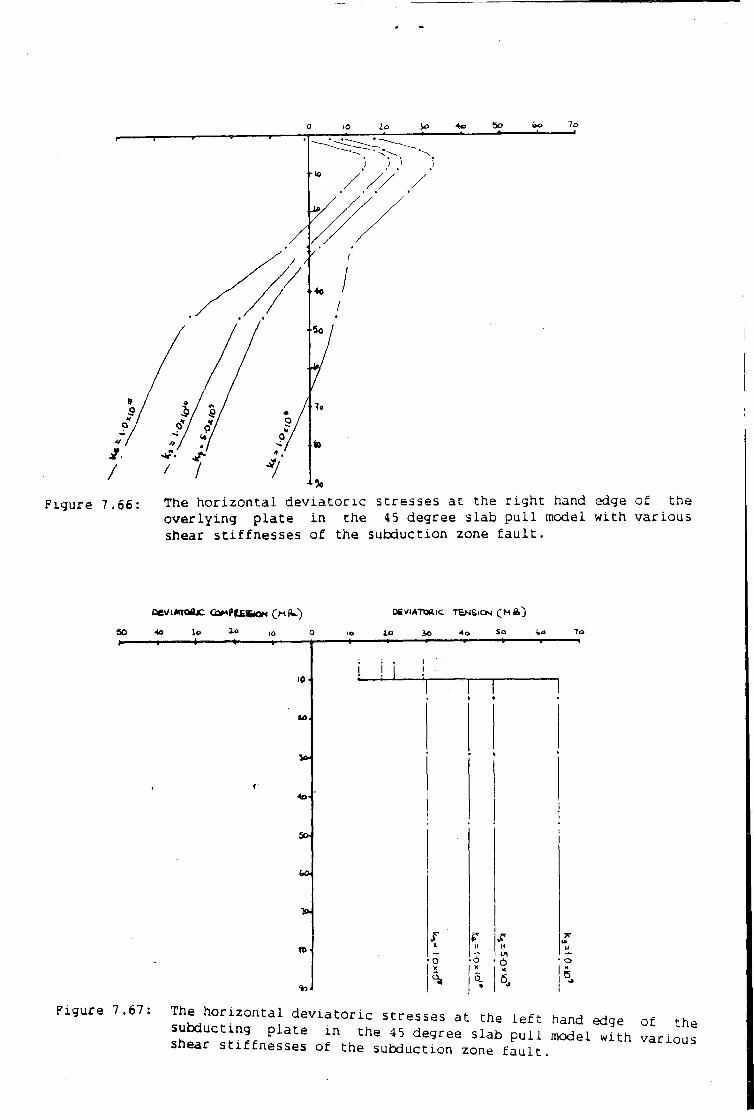
Figure 7,66: A 9o
The h o r i z o n t a l d e v i a t o r i c stresses at the r i g h t hand edge of the o v e r l y i n g p l a t e i n the 45 degree slab p u l l model w i t h v a r i o u s shear s t i f f n e s s e s of the subduction zone f a u l t .
so
D S V I A T O B . I C T E N S l C N CM BM)
>o lo Jo 4a So to 7o
• t o -
*5
I
Figure 7.67:
o X
The h o r i z o n t a l d e v i a t o r i c stresses at the l e f t hand edge of the subducting p l a t e i n the 45 degree slab p u l l model w i t n v a r i o u s shear s t i f f n e s s e s of the subduction zone f a u l t .
The reason for t h i s response can be seen i n the nodal displacements.
When the f a u l t i s locked ( f i g u r e 7.39) each dual node i s con s t r a i n e d to
have the same displacement and consequently the slab p u l l f o r c e acts
e q u a l l y to deform both the o v e r l y i n g and subducting p l a t e s . The r e s u l t of
t h i s strong coupling of the p l a t e s i s t h a t the 45 degree slab p u l l f o r c e
pushes the centre of the model to the r i g h t , which compresses the o v e r l y i n g
p l a t e and produces tensions i n the subducting p l a t e . Reducing the shear
s t i f f n e s s of the f a u l t increases the r e l a t i v e displacement on the dual
nodes so th a t the two p l a t e s s l i d e past one another ( f i g u r e s 7.68 t o 7.70).
This occurs because the h o r i z o n t a l component of the slab p u l l f o r c e acts
unequally on the two p l a t e s ; more of i t i s used to p u l l the subducting
p l a t e i n t o the mantle and less i s t r a n s m i t t e d to compress the o v e r l y i n g
p l a t e . Reducing the shear s t i f f n e s s consequently decouples the
displacement and the stresses of the two p l a t e s . The models t h e r e f o r e
suggest th a t the degree of mechanical co u p l i n g between the p l a t e s at a
subduction zone determines the amount of compression which the shear
component of the slab p u l l f o r c e transmits i n t o the o v e r l y i n g p l a t e .
I n the f i n a l model ( f i g u r e 7.62), i n which the shear s t i f f n e s s of the "[ -I
subduction zone f a u l t has been reduced t o 1.0x10 N m, the r e g i o n a l
h o r i z o n t a l compressive stress produced by the shear component of the slab
p u l l f o r c e has been reduced to less than 5 MPa. In t h i s model, however,
near surface h o r i z o n t a l compression of 25 MPa s t i l l occurs i n the o v e r l y i n g
p l a t e between the trench a x i s and the v o l c a n i c arc. This i s because the
o v e r l y i n g p l a t e i s s t i l l bending i n response to the v e r t i c a l component of
the slab p u l l f o r c e ( f i g u r e 7.70). This deformation occurs because the
high value which has been assigned t o the normal s t i f f n e s s of the
subduction zone f a u l t allows a component of the slab p u l l f o r c e to be
t r a n s m i t t e d normally across the f a u l t plane to deform the leading edge of - 139 -
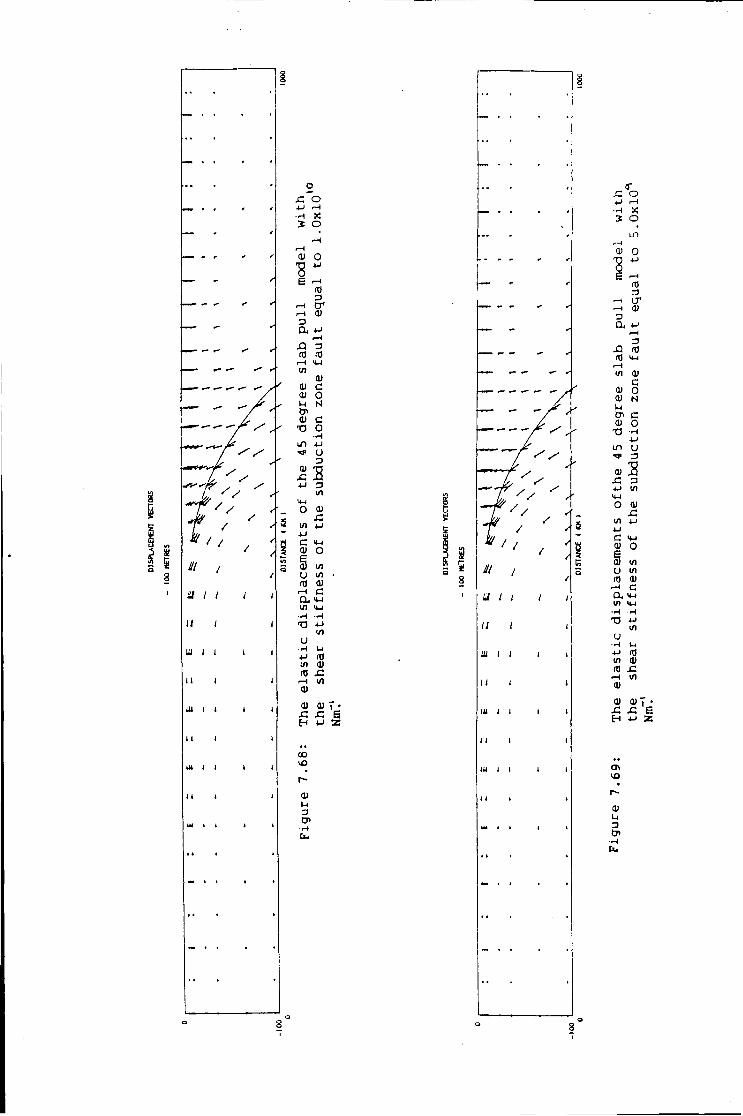
i
i l I
JIB
m i i
M i l I
xz o 4-> r- l • H
o in
i — i a) 0
"8 4 J
a i—1 IT)
•—* (T 0)
3
a, * J i — i a XI IT)
n) 14-1 •-I i/ i 0)
c 0) 0 <u N t-l
en c <D o
T 3 • H 4-1
in u •»*
0J 2 XZ 3 4-1 l / l
14-4
o 01
n l / l 4 J 4 J
c <4J
O U l
u U l IT) 01
C a <4-l i / i <t-l
• H • H
T) 4-/ U l
U • - J . 1-4 4-> TI l / l 0>
m XZ r-H U l 01
0> ar x: xz H 4-1
•
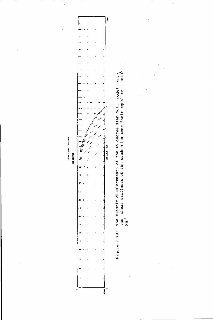
i
1 1 i
o 4-J • H s o
r-i r-( 0) o
4-1
B .—( (0 3
i - t cr 0)
3 Q , 4 J
•-( X) 3 >H <M V)
0) (1) c 01 o l-l N CP 01 c T3 o
•-( in 4 J
u 0) 3
XI i5 4-1 3 VI
*M 0 0)
x: l/l 4-1
4 J C <t-4 01 o e 0) l/l u l/l m 01
• — I c Q i >M l/l —I T> 4 J
l/l U
•H 4-> nj l/l 0) m x:
r-i
0) 01 0) x: x; H 4->
O r-t -
0) u 3 0>
• H
the o v e r l y i n g p l a t e . Reducing the shear s t i f f n e s s of the subduction zone
f a u l t t h e r e f o r e does not decrease the l o c a l h o r i z o n t a l compression which
the v e r t i c a l component slab p u l l f o r c e produces at the leading edge of the
o v e r l y i n g p l a t e .
7.5.3 Discussion
The models presented i n t h i s s e c t i o n demonstrate t h a t the r e g i o n a l
h o r i z o n t a l compression which i s t r a n s m i t t e d i n t o the back arc re g i o n by the
slab p u l l f o r c e i s s t r o n g l y c o n t r o l l e d by the mechanical c o u p l i n g between
the p l a t e s at the subduction zone f a u l t . The mocals p r e d i c t t h a t the
stress regime i n the back arc regions of subduction zones which are
s t r o n g l y coupled w i l l be more compressive than at subduction zones which
are weakly coupled. The models t h e r e f o r e e x p l a i n t h a t the degree of
mechanical coupling i s an a d d i t i o n a l f a c t o r i n e x p l a i n i n g why the stress
regime i n the back arc regions i s v a r i a b l e between d i f f e r e n t subduction
zones. These models q u a n t i t a t i v e l y demonstrate that the decoupling
hypothesis of Kanamori (1971; 1977) i s p l a u s i b l e .
An important i m p l i c a t i o n of these models i s t h a t whatever the c o u p l i n g
of the p l a t e s , near surface h o r i z o n t a l compression occurs at the leading
edge of the subducting p l a t e . This may e x p l a i n why the s t r e s s i n t h i s
region i s c o n s i s t e n t l y observed to be compressive, whatever the s t a t e of
stress i s i n the back arc basins. These models demonstrate, however, t h a t
the magnitude of the compression i s increased when the cou p l i n g between the
pl a t e s i s higher. This implies t h a t great t h r u s t earthquakes are more
l i k e l y to occur at subduction zones which are s t r o n g l y coupled than at
those which are weakly coupled. This p r e d i c t i o n helps to e x p l a i n why the
t e c t o n i c deformation of the o v e r l y i n g p l a t e i s so v a r i a b l e between
d i f f e r e n t subduction zones (Kanamori, 1977).
- 140 -
The models t h e r e f o r e e x p l a i n
subduction zones without producing
why c r u s t a l shortening can occur
r e g i o n a l h o r i z o n t a l compression.
at
7 .6 Convection In The Asthenospheric Wedge
The p o s s i b i l i t y t h a : the subducting p l a t e induces a viscous drag
convective flow i n the o v e r l y i n g a s i h ^ i a ^ . i e r i : v:edge which heats and
shears the o v e r l y i n g p l a t e was i n i t i a l l y ^ j ^ s a d by McKenzie (1969.) t o
ex p l a i n the high heat flow which i s observed i n the back arc areas of
subduction zones. Following t h i s proposal, Karig (1970; 1971a, b)
demonstrated t h a t i n the i s l a n d arcs of the Western P a c i f i c the high heat
flow coincides w i t h p r e s e n t l y or r e c e n t l y a c t i v e s i t e s of back arc
spreading. This observation s t i m u l a t e d the development of i n c r e a s i n g l y
s o p h i s t i c a t e d numerical models of the slab induced convection (Sleep and
Toksoz, 1971; Andrews and Sleep, 1974; Toksoz and B i r d , 1977; Toksoz and
Hsui, 1978) which propose th a t back arc spreading i s i n i t i a t e d and d r i v e n
by the combination of shearing and heating of the o v e r l y i n g p l a t e produced
by the viscous flow.
The hypothesis t h a t slab induced convection i n i t i a t e s back arc
spreading, however, has r e c e n t l y been challenged because the model cannot
exp l a i n the observed s p a t i a l and temporal e p i s o d i c i t y of back arc spreading
(Chase, 1978; Uyeda and Kanamori, 1979). Hsui and Toksoz i1981), however,
concluded t h a t the one a v a i l a b l e f o c a l mechanism s o l u t i o n f o r back arc
areas agrees w i t h t h e i r hypothesis (Toksoz and Hsui, 1976) th a t back arc
spreading i s i n i t i a t e d and d r i v e n by slab induced convection. This
a s s e r t i o n i s o b v i o u s l y based upon an extremely l i m i t e d data set and
t h e r e f o r e the r o l e of slab induced convection i n d r i v i n g back arc basins
remains u n c e r t a i n .
- 141 -
One of the reasons f o r t h i s u n c e r t a i n t y about the r o l e of slab induced
convection i n d r i v i n g back arc spreading i s t h a t the stress regime which i s
produced by t h i s mechanism has only been q u a l i t a t i v e l y assessed. The
so p h i s t i c a t e d models of slab induced convection, however, make q u a n t i t a t i v e
p r e d i c t i o n s about the heating and shearing of the o v e r l y i n g p l a t e . The
model of Toksoz and Hsui (1973), f o r example, p r e d i c t s t h a t f o r a slab
d i p p i n g a t 45 degrees and subducting a t 3 cm/yr the slab induced convection
c e l l w i l l exert a shear stress of 3.5 MPa on the base of the o v e r l y i n g
p l a t e and w i l l r a i s e the temperature of the base of the l i t h o s p h e r e by
250°C at 75 m i l l i o n years a f t e r the i n i t i a t i o n of subduction. These
p r e d i c t i o n . can t h e r e f o r e be used to q u a n t i f y the stress regime which i s
produced by slab induced convection.
In t h i s s e c t i o n the stress regime produced by the shearing and thermal
volume changes which are p r e d i c t e d by the model of Toksoz and Hsui (1978)
are evaluated. The r e s u l t s w i l l be used to t e s t two hypotheses. F i r s t l y ,
does the slab induced convection generate s u f f i c i e n t t e n s i o n t o i n i t i a t e
back arc spreading by f a i l u r e a t the vo l c a n i c arc ? Secondly, i s the slab
induced convection able to produce the t e n s i o n a l stress observed i n many
back arc basins, and which may d r i v e a c t i v e back arc spreading i n some
areas ?
7.6.1 E f f e c t of shear stress
The model of Toksoz and Hsui (1978) p r e d i c t s that the slab induced
convection c e l l exerts a shear stress of 3.5 MPa on the base of the
o v e r l y i n g p l a t e at subduction zones. The stress regime produced by the
a c t i o n of t h i s basal shear stress i s evaluated i n t h i s s e c t i o n .
- 142 -
The f i n i t e element mesh i s d e s c r i b e d i n s e c t i o n 7.2. The s i d e s o f
t h i s model were c o n s t r a i n e d f o r z e r o h o r i z o n t a l d i s p l a c e m e n t and t h e base
was assumed t o be u n d e r l a i n by a f l u i d a s t h e n s o p h e r e w i t h a d e n s i t y o f
3300 kg m~ . A b a s a l shear s t r e s s o f 3.5 iMPa was a p p l i e d t o t h e 260 km l o n g
base o f t h e o v e r l y i n g p l a t e shown i n f i g u r e 7.71. The s u b d u c t i o n zone
f a u l t was assumed t o be l o c k e d .
The e l a s t i c s o l u t i o n i s shewn i n L ^ j r e , 7.72 t o 7.75. The b a s a l
shear s t r e s s has two e f f e c t s . The f i r s t i s t h a t i t d i s p l a c e s t h e c e n t r e o f
t h e model t o t h e l e f t w hich produces a r e g i o n a l h o r i z o n t a l c o m p r e s s i o n o f
4 MPa i n t h e s u b d u c t i n g p l a t e and a r e g i o n a l h o r i z o n t a l c o m p r e s s i o n o f a
s i m i l a r magnitude i n t h e o v e r l y i n g p l a t e . The second i s t h a t i t i n d u c e s a
b e n d i n g moment which causes an upwards f l e x u r e o f t h e model a b o u t an a x i s
above t h e base o f t h e s u b d u c t i o n zone f a u l t , and a downwards f l e x u r e a t t h e
r i g h t hand edge o f t h e model ( f i g u r e 7.76). The upward f l e x u r e produces
near surfafce h o r i z o n t a l t e n s i o n s o f 4 MPa w i t h u n d e r l y i n g c o m p r e s s i o n s o f
10 MPa, and t h e downward f l e x u r e produces near s u r f a c e s t r e s s e s o f z e r o
w i t h u n d e r l y i n g h o r i z o n t a l t e n s i o n s o f 14 MPa. The e f f e c t s o f t h e b e n d i n g
moment t h e r e f o r e d o m i n a t e s t h e s t r e s s regime i n t h e o v e r l y i n g p l a t e . The
s t r e s s a s s o c i a t e d w i t h i t , however, i s i n s u f f i c i e n t t o cause f a i l u r e
anywhere i n t h e model.
The shear s t r e s s produced by s l a b i nduced c o n v e c t i o n i s a ren e w a b l e
source o f s t r e s s , as l o n g as s u b d u c t i o n c o n t i n u e s , and t h e r e f o r e t h e above
model was a l l o w e d t o r e l a x v i s c o - e l a s t i c a l l y f o r 5 m i l l i o n y e a r s . The
r e s u l t s o f t h i s a n a l y s i s a r e shown i n f i g u r e s 7.78 t o 7.81. The major
d i f f e r e n c e between t h i s and t h e e l a s t i c s o l u t i o n i s t h a t t h e r e g i o n a l
c o m p r e s s i o n and t e n s i o n has been a m p l i f i e d i n - t h e e l a s t i c l a y e r s , b u t t h e
superimposed f l e x u r a l s t r e s s e s a r e u n a l t e r e d and a r e c o n s e q u e n t l y l e s s
- 143 -
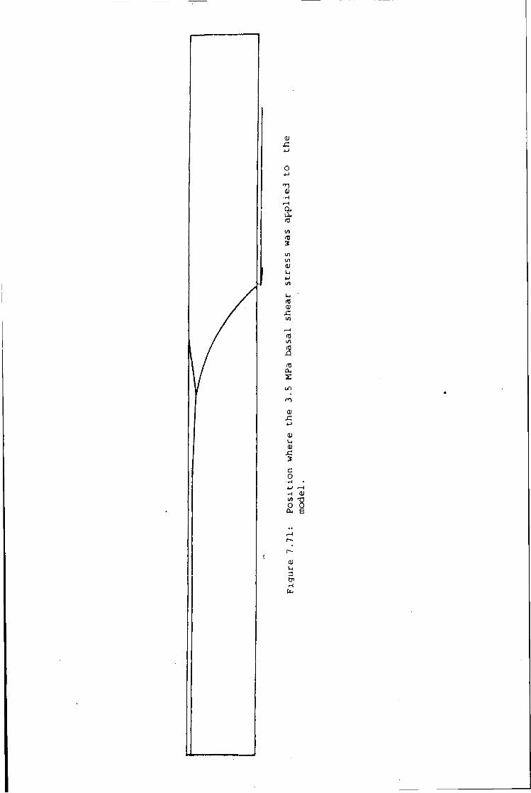
"1 0)
•H <—( a
1/1
3
0)
1-J
01 i/l
rtJ i/i
01
0) u OJ sz
c o 01
"8
r— <V u a CP
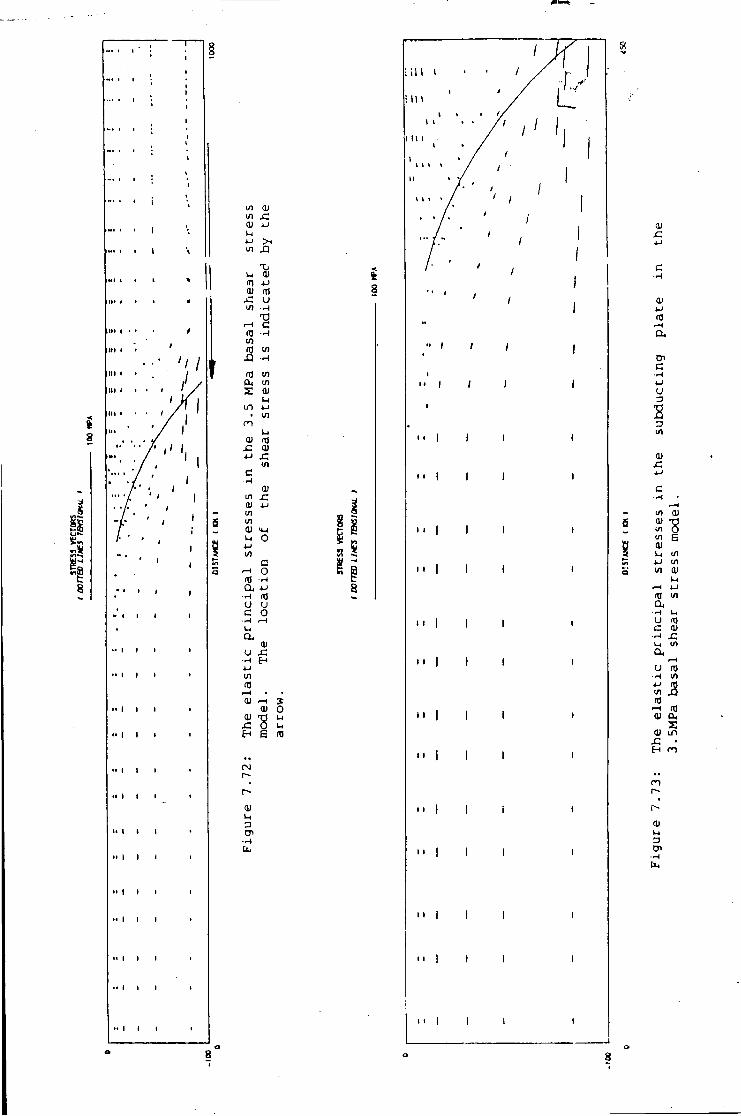
I l l I
I I I I
( I I
> l l i
Ul Ul
4-1 U 4J >1 Ul XI
T . u ai m * J 01 m jZ u l/l
XI r H c nj •r4 ui (3 1/1 J3 •rH
nj Qu X ai
u m 4-1 • Ul
0) HJ £ ai . c Ul
C (D
I/l r: Q) 4-> </> in 01 t-i o i-> Ul
c r—1 o
- I a * J
•H u u c o
•H >—1
a
u •W
ui (TJ i—i • a) 1—1
a)
r-
P
CP
O
"8 £
8
U H
8
n | | I
| | I I I
i i I I I
M i l I
H I I i
II I I I
H I I i
H I I
I I I I I
4-1
c r-l
Ul 0) a> i/i 0 Ul s ai u Ul 4-1 U) Ul a)
u r-l 4-1 m Ul a •H t-i u c 01
•r-l jC 1-1 Ul a ,
»—i u ID
•H Ul 4-1 <s Ul m
>-( as 01 &
(U in . c • H
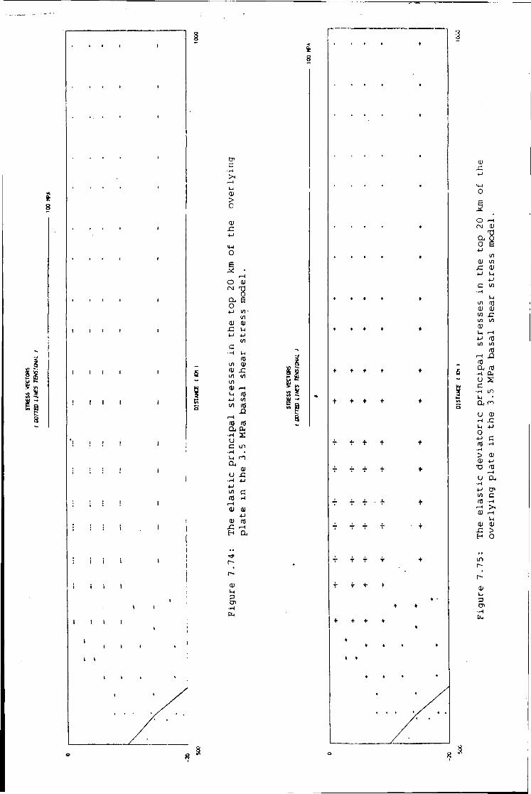
8
i i i i
i i i i
i I l l
I I I I
5
CP c -I—J
>• <-H
ai > c o>
a o
f
<—i o (N T? CL u E O
i/i • in
01 ai u
t-J u l/l c
•H m
in a> ai x: l/l </i 1/1 a> u m *-i in i/i
.—1 ITJ m a a< H U c in
- H • l-i a,
0) u C
• H 4-1 1/1 c <T> •H
r H <U 01
4 J o> m
rH H a
•ST
r~ t-»
0) u
tn
p
t • • •
• t • •
+ + + +
+ + +
+ +
+ + • •
0)
e O rH (N 01
0 e 4-1
1/1 01 in
C 0) 4-J U
4-1 C in
• H u
in in 01 01 l/l £ 1/1 l/l 0) U rH 4J 03 l/l l/l
it) ITJ a , m H cu u x c -H LO
CL
U 01 •H" JC l-l 4-> o 4 J C aj H
•H > 0) 01 4-J TD m
rH U CL
•H 4-1 en in c (0 H
rH > 0) rH
01 0) c > H O
in
u 3 •H
I I I * • »
• « •
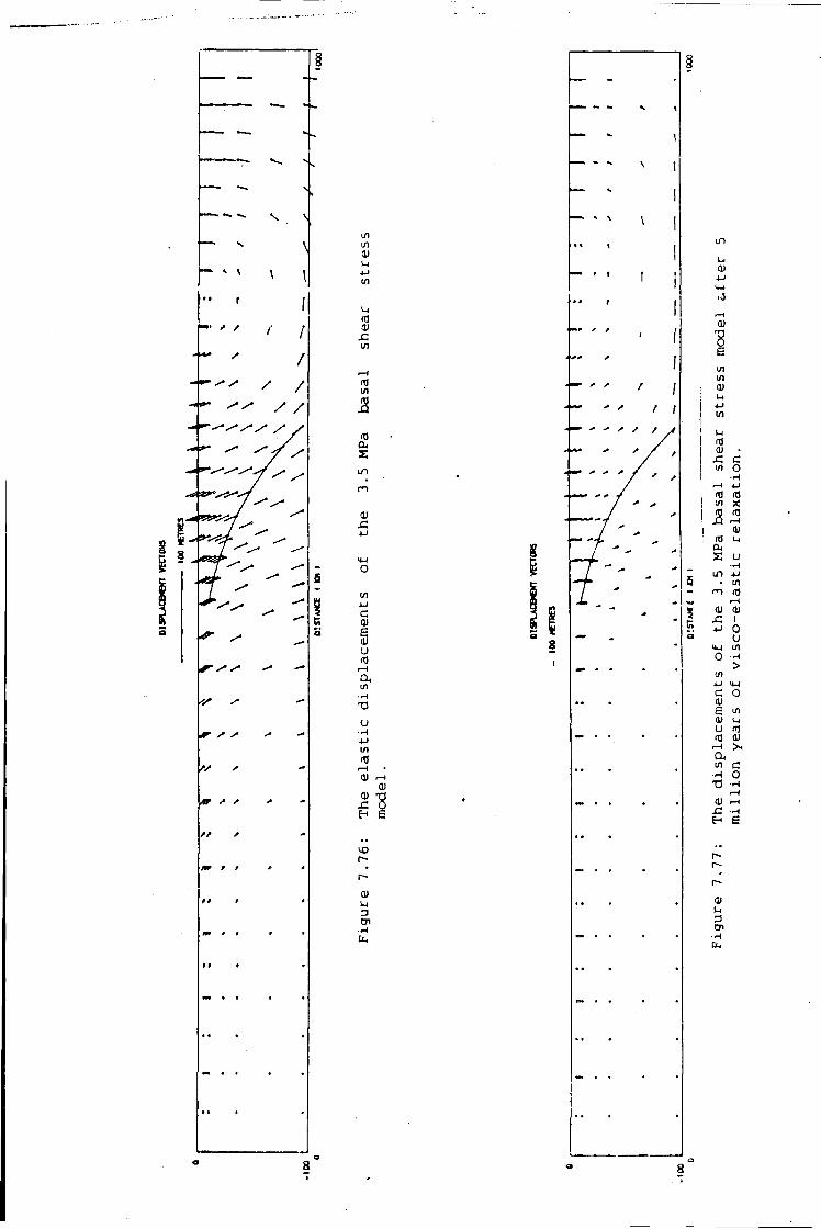
m 1/1 0) u
u
£ in
in
3
c 01 e 0)
u
a 1/1
•H
-a u i/i
i-H 01 Q) J! "8
r-
0)
Cn
1/1
u 01 4-J U-l
.0 r—1 0)
0 e t/i I/I 01 u in u m o> •
c in o
•H ^ - i 4-J rfl m i/l x a <o
r-H
0> u
a. s u
•H
in 4-1 • Ul
C I m i—i 01 £ i 0 u w o > 1/1
c o 01 s in 0) ( J in rfl <D ,-1 a, in c
•H 0 T3 •H
.-1 0) r-t
H 6
r-r-r-
01
3 •H
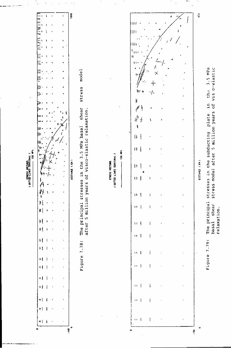
Ill III
Ml
I I I
«l Hi M l
I 1
I •
t •
\ \
I
\
ii» • *
I •
HI I
»l I
" I I
••I I
••I I
"8 6 m m 0)
u • rO c 0) 0 U] •u
(0 r-H « rd 1/1 ai
u u
(t) (X 4-1 z: in
rO in i-< 0) ro 1
o m u
in 4-1
> c •.-1 4-1
0 Ul 0) l/l Ul u Ul m (U aj t-4 >i 4-i l/l c
o r-H r0 i—1 -•H •rJ U E c —4 in 1-1
u a) 4-1
m
00
ai 1-4 D
3 8
-5 *
..V -/• \
11
" I
11
ro u a, —1
4-1 1/1
in r0 r-l
ro 01 1 o Ul
4-> •H
> c 1 o
Ul ai i-. 4-1 (0 <0 a)
>1 a
c o
CP •H c r-H
r-4 4-1 •H U £ 3 m
3 in <D
4J 0)
(0 4-1
r~l c •H "8 in 6 0) i/i ui in Ul 0) CD u i-i 4-J 4-> 1/1 Ul
ra i-i a , m • •H 0) c u . c o C U) -H -H 4-1 u rd
rO (0 II III H
£ rd a) E-I ia u r-
ai 3 (Ji
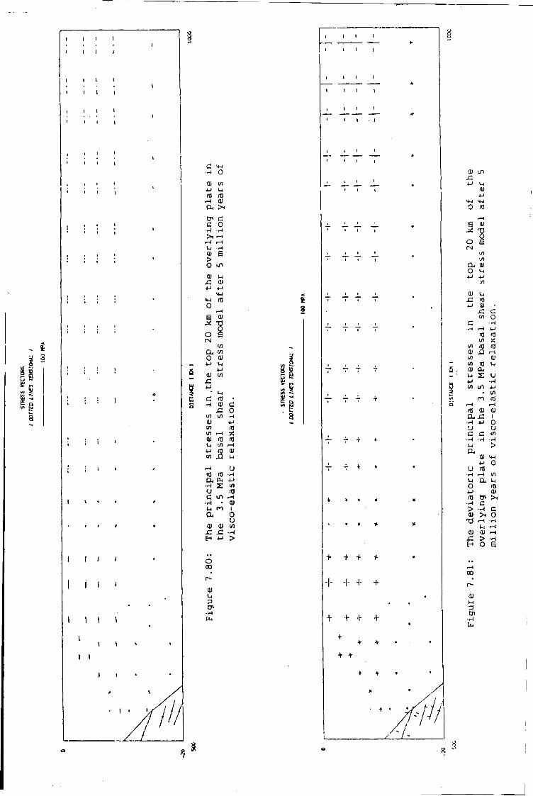
c —I 0 0) in 4-1 u m m «—i 01 a >>
cn c c 0 •H •H
.-1 i—i —\ E
> o in 01 u
x: 0) 4-1 4->
•4-1 m
O i—i
E 0)
"8 o u
E CM
Ul a , i/i 0 01 4-> lH
4-1 0) Ul
4J u
c fO • —t 01 c
x: 0 l/l Ul —I 0) 4-1 l/J IT) 1/1 t -H X 01 m a) u 1/1 r - l 4-1 m 01
XI u r - l u
(0 a , CU 4-> •-i l/l u <TJ c in i-H •H • 0) Ul 1 a , 0
u 0) 01 Ul x: x: H 4-1 >
o CO
01 u a CP
T T T
T T »
— r + *
+ • « «
• * *
+ + + +
-|- -I- + +
+ + + +
+ + + + +
p r o m i n e n t . D e s p i t e t h i s s t r e s s a m p l i f i c a t i o n , however, f a i l u r e i s n o t
p r e d i c t e d anywhere i n t h e model.
These r e s u l t s d e m o n s t r a t e t h a t t h e shear s t r e s s p r e d i c t e d by t h e s l a b
i n d u c e d c o n v e c t i o n model o f Tokscz and Hsui (1973) produces h o r i z o n t a l
t e a s i o n a l s t r e s s e s i n t h e back a r c area o f s u b d u c t i o n zones. The model
" t h e r e f o r e agrees w i t h t h e s u g g e s t i o n o f t h a se a u t h o r s t h a t t h i s f o r c e can
h e l p t o d r i v e back a r c s p r e a d i n g and can account f o r t h e t e n s i o n commonly
ob s e r v e d i n t h e s e r e g i o n s . The magnitude o f t h e t e n s i o n a l s t r e s s , however,
i s i n s u f f i c i e n t t o cause f a i l u r e o f t h e l i t h o s p h e r e and t h e r e f o r e c a n n o t
s o l e l y a c c o u n t f o r i n i t i a t i o n o f back a r c s p r e a d i n g . I n o r d e r f o r t h e
b a s a l shear s t r e s s t o cause f a i l u r e i t would t h e r e f o r e e i t h e r have t o be o f
a l a r g e r magnitude o r a c t over a g r e a t e r d i s t a n c e . A much more f u n d a m e n t a l
problem, however, i s t h a t t h e v o l c a n i c a r c i s i n c o m p r e s s i o n and t h e r e f o r e
t h i s mechanism cannot a c c o u n t f o r why t h e back a r c s p r e a d i n g i s i n i t i a t e d
by f r a c t u r e a t t h e v o l c a n i c a r c . *
The s l a b i n d u c e d c o n v e c t i o n causes t h e o v e r l y i n g p l a t e t o be d i s p l a c e d
towards t h e t r e n c h , i . e . t o o v e r r i d e t h e s u b d u c t i n g p l a t e . T h i s s u p p o r t s
t h e p r o p o s a l o f R i c h t e r (1973) t h a t t h i s f o r c e c o n t r i b u t e s towards t h e
t r e n c h s u c t i o n e f f e c t . The model, however, i n d i c a t e s t h a t t h e c o n t r i b u t i o n
would be r e l a t i v e l y s m a l l u n l e s s t h e b a s a l shear s t r e s s i s much l a r g e r .
7.6.2 E f f e c t o f t h e r m a l volume changes
The model o f Toksoz and Ksui (1978) p r e d i c t s t h a t a f t e r 75 m i l l i o n
y e a r s t h e s l a b i n d u c e d c o n v e c t i o n c e l l causes a 250 C h e a t i n g o f t h e base
of t h e o v e r l y i n g p l a t e . The s t r e s s regime produced by t h e r e s u l t i n g
t h e r m a l volume changes a r e m o d e l l e d i n t h i s s e c t i o n .
- 144 -
The f i n i t e element mesh i s d e s c r i b e d i n s e c t i o n 7.2. The s i d e s o f
t h i s model were c o n s t r a i n e d f o r z e r o h o r i z o n t a l d i s p l a c e m e n t and t h e base
was assumed t o be u n d e r l a i n by a f l u i d a s t h e n o s p h e r e w i t h a d e n s i t y o f
3300 kg m"3
The t e m p e r a t u r e anomaly ( f i g u r e 7.82) whi c h was used i n t h e f i n i t e
element c a l c u l a t i o n s i s c y l i n d r i c a l , w i t h i t s a ^ i s p e r p e n d i c u l a r t o t h e
s t r i k e , and has i t s c e n t r e ( x c , y c ) a t (780.0 km, -123.239 km). The
t e m p e r a t u r e r i s e , T, a t a p o i n t ( x j , , y ^ ) i n t h e o v e r l y i n g p l a t e was
c a l c u l a t e d f r o m t h e f u n c t i o n
T = • e
where 2,, t h e t h i c k n e s s o f t h e l i t h o s p h e r e was t a k e n as 95 km, ^T^,, t h e
t e m p e r a t u r e r i s e o f t h e base was assumed t o be 250°C, and r ^ , t h e r a d i a l
d i s t a n c e t o t h e p o i n t p was c a l c u l a t e d from t h e e x p r e s s i o n
^ = / ( x j , - x c ) * + (vP-yc )*v
T h i s t e m p e r a t u r e anomaly a p p r o x i m a t e s t h a t i n t h e model o f Toksoz and
Hsui ( 1 9 7 8 ) . The t h e r m a l s t r e s s e s were c a l c u l a t e d u s i n g t h e i n i t i a l s t r a i n
method ( s e c t i o n 3.8) assuming t h a t t h e volume c o e f f i c i e n t o f e x p a n s i o n , * * ,
i s 1 . 0 x l 0 ~ *
The e l a s t i c s o l u t i o n u s i n g t h i s model i s shown i n f i g u r e s 7.83 t o
7.86. These r e s u l t s d e m o n s t r a t e t h a t t h e t h e r m a l volume changes w h i c h a r e
produced by a h e a t i n g o f t h e o v e r l y i n g p l a t e by a s l a b i n d u c e d c o n v e c t i o n
c e l l has two e f f e c t s . The f i r s t i s t o i n d u c e a f l e x u r e o f t h e o v e r l y i n g
p l a t e w i t h an a x i s a t t h e c e n t r e o f t h e t e m p e r a t u r e anomaly ( f i g u r e 7 . 8 7 ) .
- 145 -
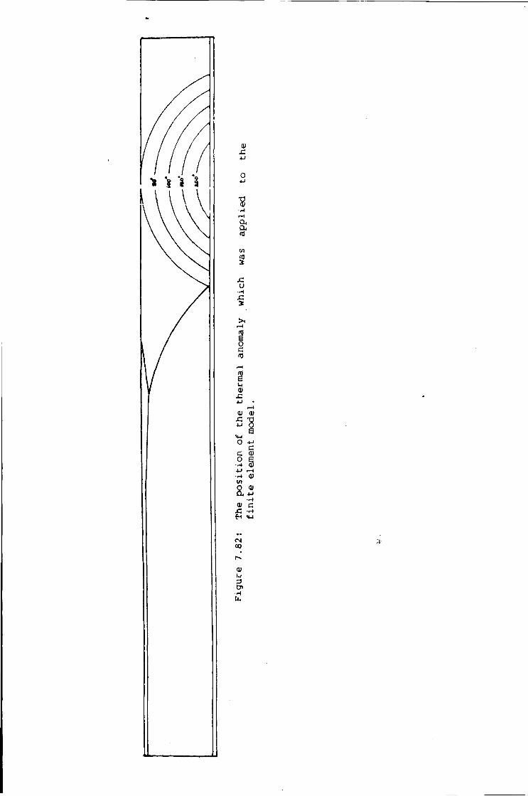
0)
3 a, a m
i/i 2
u
f0 E o c
t-i
0> 0)
s O 4-1 c C 01 2 § 4-1 i-H r4, 0)
O 0) a 4-i
a» c H "4-1
CM CO
0)
o o
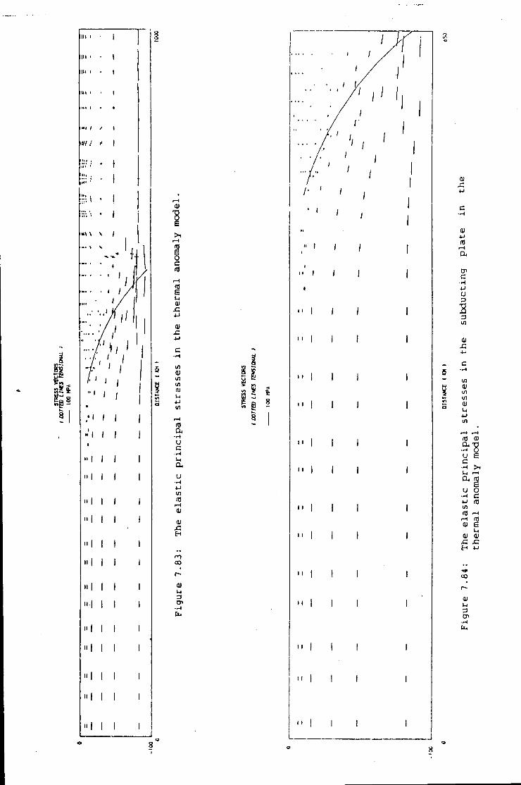
1 in i
in >
in i
in i"
/ it
-8 0) M
CP i'
u 3 2 01
11 01
01
Ul
Ul in i Ul o> 8 Ul
Ul 8 in 8 o> 8 ! ! Ul
a -(0 01 " a. •8
a, a, u o Ul
(0 u m Ul 01
01 Oi S
0< 0> «
00
" CO
01
01 I .
»
•«
8
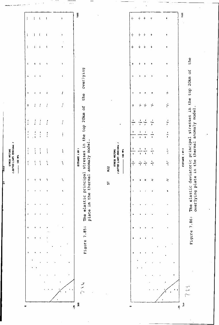
I. I
i I I
I 1 I I
I I I I
I I I I
• I I I
i i ' '
I I I !
I i I '
1 1 1 »
I I I
CP c
> o
01
0
Ej J2 o
a . o •u 01 x: 4-1 •
1—( c "8
Ul 6 01 1/1 >i Ul rH 01 ro Ul £ 4-1 O Ul c
rd r-4 rd i—i a , rd £ u Ul c 0) •r-l x: Ul 4J a
01 u JZ
4J 4-1 Ul e rd i—i 01 01
4-1 01 id
i-i H a ,
in oo
0) Ul 3 CP
T T T +
T T T +
+ + + •
» * 4 *
• * + •
I I I I
I I I I
I I I I
I I I I
I I I I
I I I I
I I » I
I I I I
• » t
0 6
o CM
a o 4J
01 r. 4->
c r-l •H 0) U) Q 0) Ul Ul 01 r-l Ui rd 4-> £ Ul O
c 1—1 rd rd a , -4 •r-i a) u E c u -H 11 Ul JC CLi 4J
( J 0) -4 Ul 4-1 O 4-1 d rd •p-i -r-l
> at 0) 4J T3 rd
r-l U a , •r-1 4-1 cn Ul c rd r-t > i 01 r-H
Ul 01 0) -C > E-i o
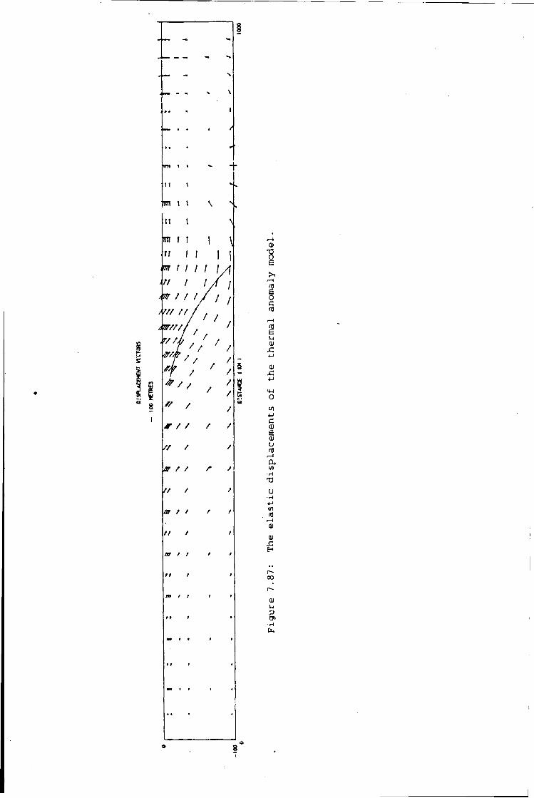
MM
mi
It m 1 t
0)
"8 W i l l i /
(0 >vr r t ! I J
/ / / /
.r/ / /
(1)
/
5 r H a. 1/1
at ft
m f
it CO
m 0)
8
T h i s f l e x u r e produces a h o r i z o n t a l t e n s i o n o f 62 MPa a t t h e t o p o f t h e
c r u s t and a h o r i z o n t a l c ompression of 130 MPa a t t h e base o f t h e
l i t h o s p h e r e . I t i s p r e d i c t e d from t h e s e s t r e s s e s t h a t f a i l u r e w i l l o c c u r
a t 1 km d e p t h i n t h e element above t h e c e n t r e o f t h e t e m p e r a t u r e anomaly.
F a i l u r e i s n o t p r e d i c t e d anywhere e l s e i n t h e model. The second e f f e c t i s
t h a t t h e t h e r m a l e x p a n s i o n o f t h e o v e r l y i n g p l a t e produces a r e g i o n a l
h o r i z o n t a l compression o f 60 MPa i n t h e s u b d u c t i n g p l a t e and t h e r e g i o n o f
the o v e r l y i n g p l a t e above t h e s u b d u c t i o n zone f a u l t . T h i s c o m p r e s s i o n
r e s u l t s f r o m t h e z e r o h o r i z o n t a l d i s p l a c e m e n t boundary c o n d i t i o n a p p l i e d t o
th e l e f t hand edge o f t h e model. Because c o m p r e s s i v e s t r e s s o f t h i s
magnitude i s not observed, a t s u b d u c t i o n zones i t i s c o n c l u d e d t h a t t h i s
boundary c o n d i t i o n i s u n r e a l i s t i c .
These r e s u l t s d e m o n s t r a t e t h a t t h e t e m p e r a t u r e anomaly whi c h i s
produced by t h e s l a b i n d u c e d c o n v e c t i o n model o f Toksoz and Hsui (1978)
causes t h e r m a l volume changes w h i c t i p roduce near s u r f a c e h o r i z o n t a l
t e n s i o n a l s t r e s s e s i n t h e back a r c a r e a o f s u b d u c t i o n zones. The model
p r e d i c t s t h a t t h e se s t r e s s e s w i l l be a maximum above t h e c e n t r e o f t h e
t e m p e r a t u r e anomaly and t h e r e f o r e agrees w i t h t h e h y p o t h e s i s t h a t t h e
t e n s i o n d r i v i n g back a r c s p r e a d i n g can be produced by t h e t h e r m a l e f f e c t s
o f s l a b i n d u c e d c o n v e c t i o n . The model, however, does n o t a g r e e w i t h t h e
t h e h y p o t h e s i s t h a t back a r c s p r e a d i n g i s i n i t i a t e d by t h e t h e r m a l e f f e c t s
of s l a b i n d u c e d c o n v e c t i o n because t e n s i o n a l s t r e s s e s a r e n o t p r e d i c t e d i n
t h e r e g i o n o f t h e v o l c a n i c a r c .
7.6.3 D i s c u s s i o n
The models which have been p r e s e n t e d i n t h i s s e c t i o n show t h a t b o t h
the b a s a l shear s t r e s s and t h e t h e r m a l volu.ne changes produ c e near s u r f a c e
h o r i z o n t a l t e n s i o n a l s t r e s s e s i n t h e back a r c area o f s u b d u c t i o n zones.
- 146 -
The model t h e r e f o r e s u p p o r t s t h e h y p o t h e s i s t h a t s l a b i n d u c e d c o n v e c t i o n
can cause t e n s i o n a l t e c t o n i c s i n t h e o v e r l y i n g p l a t e and c o n s e q u e n t l y may
p r o v i d e the t e n s i o n t o d r i v e back a r c s p r e a d i n g .
Both t h e b a s a l shear s t r e s s and t h e t h e r m a l volume changes, however,
g i v e r i s e t o e i t h e r c o m p r e s s i o n or low magnitude t e n s i o n m t h e v i c i n i t y o f
t h e v o l c a n i c a r c . T h a s j r e s u l t s t h e r 3 f o r e suggest t h a t back a r c s p r e a d i n g
i s n o t i n i t i a t e d by t h e s l a b i n d u c e d c o n v e c t i o n c e l l , c o n t r a r y t o t h e
h y p o t h e s i s o f Toksoz and Hsui ( 1 9 7 3 ) . Back a r c s p r e a d i n g must t h e r e f o r e be
i n i t a t e d by some o t h e r mechanism as has been proposed by o t h e r a u t h o r s
(Chase, 1978; Uyeda and Kanamori, 1979). Once back a r c s p r e a d i n g has been
i n i t i a t e d , however, t h e s l a b i n d u c e d c o n v e c t i o n c e l l can p r o v i d e a d d i t i o n a l
t e n s i o n t o d r i v e t h e s p r e a d i n g .
The models which have been p r e s e n t e d i n t h i s s e c t i o n assume a
s u b d u c t i o n r a t e o f 1 cm/yr and a d i p o f 45 d e g r e e s . A l t h o u g h t h e s e v a l u e s
a r e r e p r e s e n t a t i v e o f s e v e r a l s u b d u c t i o n zones t h e r e a r e some i m p o r t a n t
d e v i a t i o n s f r o m t h i s , n o t a b l y t h e Marianas where t h e d i p i s 80 d egrees and
t h e C h i l e area where t h e d i p i s about 20 d e g r e e s . I t was, however, n o t
p o s s i b l e t o q u a n t i t a t i v e l y examine t h e e f f e c t o f v a r y i n g t h e s e p a r a m e t e r s .
An a d d i t i o n a l l i m i t a t i o n o f t h e models o f t h e t h e r m a l anomaly i s t h a t
i t has been assumed t h a t t h e t h e r m a l s t r e s s e s a f t e r 75 m i l l i o n y e a r s can be
e v a l u a t e d u s i n g an e l a s t i c s o l u t i o n . Thermal s t r a i n s , however, may be
r e l i e v e d by c r e e p o v e r a much s h o r t e r p e r i o d because t h e y a r e
non-renewable. The model o f s e c t i o n 7.6.2 c o n s e q u e n t l y r e p r e s e n t s t h e
maximum s t r e s s which c o u l d be produced by t h e t e m p e r a t u r e anomaly.
Another l i m i t a t i o n i s t h a t u s i n g t h e z e r o d i s p l a c e m e n t boundary
c o n d i t i o n a t t h e edges o f t h e model r e s u l t s i n t h e development o f
- 147 -
u n r e a l i s t i c a l l y l a r g e compressions i n t h e s u b d u c t i n g p l a t e . A more
r e a l i s t i c s o l u t i o n c o u l d p o s s i b l y be o b t a i n e d i f t h e l e f t hand boundary was
u n c o n s t r a i n e d .
The f i n a l l i m i t a t i o n o f t h e models i s t h a t t h e y n e g l e c t t h e s t r e s s
produced by i s o s t a t i c a l l y compensated l o a d i n g o v e r t h e h o t , low d e n s i t y
r e g i o n in t h e back a r c a r e a s . T h i s may oe a s i g n i f i c a n t source o f t e n s i o n
i n back a r c b a s i n s .
7.7 Summary And C o n c l u s i o n s
A c o n s i s t e n t s t r e s s regime i s p r e d i c t e d i n t h e s u b d u c t i n g p l a t e and i n
t h e p o r t i o n o f t h e o v e r l y i n g p l a t e between t h e t r e n c h a x i s and t h e v o l c a n i c
a r c i n a l l o f t h e models wh i c h have a s l a b p u l l f o r c e a p p l i e d t o them.
T h i s s t r e s s regime i s h o r i z o n t a l t e n s i o n i n t h e s u b d u c t i n g p l a t e and
h o r i z o n t a l c o m p r e s s i o n i n t h e o v e r l y i n g p l a t e . I t has been stiown t h a t t h i s
s t r e s s system i s p r e d i c t e d whatever t h e a n g l e o f t h e s l a b p u l l f o r c e , t h e
degree o f m e c h a n i c a l c o u p l i n g o f t h e p l a t e s or t h e magnitude o f t h e s l a b
p u l l f o r c e a r e assumed t o be. The c o n s i s t e n c y o f t h e s e s t r e s s e s i m p l i e s
t h a t t h e l a t e r a l v a r i a t i o n i n t h e h o r i z o n t a l s t r e s s w h i c h i s o b s e r v e d i n
these r e g i o n s a t a l l s u b d u c t i o n zones i s produced by t h e s l a b p u l l f o r c e .
I t has, however, been shown t h a t t h e magnitude o f t h e h o r i z o n t a l s t r e s s Magnitude
which i s produced by t h e s l a b p u l l f o r c e i s dependent upon t h e ^ o f t h e
s l a b p u l l f o r c e , i t s d i p and t h e degree o f m e c h a n i c a l c o u p l i n g o f t h e
p l a t e s . The o b s e r v e d v a r i a t i o n i n t h e d i p o f t h e s l a b and t h e d e g r e e o f
m e c h a n i c a l c o u p l i n g between t h e p l a t e s , t h e r e f o r e , p r o b a b l y e x p l a i n s t h e
observed v a r i a t i o n i n t h e t e c t o n i c d e f o r m a t i o n a t t h e l e a d i n g edge o f t h e
o v e r l y i n g p l a t e a t d i f f e r e n t s u b d u c t i o n zones.
The s t a t e of stress i n back arc areas, however, has been shown to be
v a r i a b l e . Both h o r i z o n t a l tension and compression can occur. H o r i z o n t a l
tension i s produced at a c t i v e c o n t i n e n t a l margins by the i s o s t a t i c a l l y
compensated loading of the cruse. Local h o r i z o n t a l t e n s i o n i s also
produced by heating and shearing associated w i t h slab induced convection
wherever the subducted slab penetrates deeper than a few hundred
k i l o m e t r e s . Renewable h o r i z o n t a l tension may also be generated by
i s o s t a t i c a l l y compensated loading r e s u l t i n g ' from the hot, low d e n s i t y
mantle associated w i t h slab induced convection. The t e n s i o n a l stress from
these sources not be expected to vary g r e a t l y i n magnitude between
d i f f e r e n t subduction zones. Regional h o r i z o n t a l compressive stress a r i s i n g
from the slab p u l l f o r c e may be superimposed upon these t e n s i o n a l stresses.
Their magnitude, however, i s dependent upon :he d i p and the magnitude of
the slab p u l l f o r c e . Unlike the t e n s i o n a l stresses, however, the amount of
compression which i s t r a n s m i t t e d i n t o t h i s region i s s t r o n g l y c o n t r o l l e d by
the degree of mechanical co u p l i n g of the p l a t e s at the subduction zone
f a u l t . The models t h e r e f o r e demonstrate t h a t the s t a t e c f s t r e s s i n back
arc areas i s c r i t i c a l l y dependent upon the l o c a l i n t e r p l a y between the
processes producing tension and compression. This may e x p l a i n why the
stress regime i s observed to be so v a r i a b l e i n back arc areas.
An important i m p l i c a t i o n of the models i s t h a t the l a r g e s t magnitude
t e n s i o n a l stresses, and t h e r e f o r e the most favourable c o n d i t i o n s f o r the
development of a c t i v e l y spreading back arc basins, w i l l be developed where
the d i p of the slab p u l l f o r c e i s high and/or the p l a t e s are decoupled at
the subduction zone f a u l t . This p r e d i c t i o n i s i n good agreement w i t h
observations (Uyeda and Kanamori, 1979). The models do not, however,
provide a c l e a r explanation of how back arc spreading can be i n i t i a t e d by
f a i l u r e at the volcanic arc. One p o s s i b i l i t y i s that the compression i n
- 149 -
t h i s region i s reduced as a r e s u l t of a decoupling of the p l a t e s at the
subduction zone f a u l t so th a t the t e n s i o n a l stresses produced by the short
wavelength load of the volca n i c arc can produce f r a c t u r e i n the c r u s t . An
a l t e r n a t i v e e x p l a i n a t i o n i s t h a t the dynamics of the subduction process,
which i n c l u d e r o l l - b a c k (Chase, 1978; Molnar and Atwater, 1978) and the
un d e r t h r u s t i n g r e s u l t i n g from subduction zone earthquakes ',Melosh and
F l e i t o u t , 1982) could i n i t i a t e the f r a c t u r e . The f a c t o r s which cause the
i n i t i a t i o n c; back arc spreading t h e r e f o r e remain a major o u t s t a n d i n g
problem.
The models also make two proposals about the o r i g i n of the trench
suction f o r c e . F i r s t l y , they suggest t h a t t h i s a r i s e s from the l a t e r a l
pressure v a r i a t i o n s at a subduction zone. This occurs because the trench
i s a low pressure region and the o v e r l y i n g c r u s t a high pressure r e g i o n .
This pressure grad i e n t causes diplacement of the high pressure o v e r l y i n g
p l a t e i n t o the low pressure trench. The e f f e c t of t h i s displacement i s t o
induce h o r i o n t a l d e v i a t o r i c tensions i n the c r u s t of the o v e r l y i n g p l a t e .
These stresses would be expected t o be renewable as long as the trench
remains and t h e r e f o r e could e x p l a i n why t h i s f a c t o r i s r e q u i r e d i n a l l of
the models of the p l a t e t e c t o n i c d r i v i n g f o r c e . An a d d i t i o n a l , although
much lower magnitude, e f f e c t i s the renewable shear stress produced by the
slab induced convection c e l l .
The demonstration t h a t the l a t e r a l d e n s i t y v a r i a t i o n s a t a c t i v e
c o n t i n e n t a l margins produces a s i m i l a r e f f e c t to the trench s u c t i o n force
has an important i m p l i c a t i o n f o r the c o n t i n e n t a l s p l i t t i n g mechanism. This
i s because i t i s g e n e r a l l y considered t h a t Pangea was almost completely
surrounded by a c t i v e c o n t i n e n t a l margin subduction zones. The subducted
p l a t e i n these regions would probably have a steep d i p because i t would not
- 150 -
be a c t i v e l y o v e r r i d e n by the supercontinent. I n t h i s s i t u a t i o n che
compression t r a n s m i t t e d i n t o the o v e r l y i n g p l a t e would be of a low
magnitude so t h a t the trench suction force could cause the tension r e q u i r e d
to m i t i t i a t e c o n t i n e n t a l s p l i t t i n g ( B o t t , 1982b).
In conclusion, the models are important i n demonstrating t h a t c r u s t a i
shortening can occur at Subductlcn zones without n e c e s s a r i l y producing
r e g i o n a l compression i n the o v e r l y i n g p l a t e . They e x p l a i n t h a t t h =
observed l a t e r a l v a r i a t i o n i n stress across the subducting p l a t e and the
o v e r l y i n g p l a t e i s caused by the combined e f f e c t of l a t e r a l d e n s i t y
v a r i a t i o n s and the slab p u l l f o r c e . The v a r i a t i o n i n s t r e s s across the
back arc region of subduction zones, however, has been explained i n terms
of the l o c a l balance of the forces producing tension and compression and
the mechanical coupling of the p l a t e s a t the subduction zone f a u l t .
The models developed i n t h i s chapter have t h e r e f o r e gone some way
towards e s t a b l i s h i n g the major sources of stress a t a general subduction
zone. Future analyses should concentrate on analysing the stress produced
by these forces at p a r t i c u l a r examples of subduction zones.
Despite tha general success of the models which have been presented i n
t h i s chapter there are some shortcomings of the present a n a l y s i s . These
are:
1. The bending stress a r i s i n g from the f l e x u r e of the subducting
p l a t e have not been modelled. These stresses would be
superimposed upon the stress regime modelled i n the subducting
p l a t e and would t h e r e f o r e l o c a l l y modify the stress regime.
- 151 -
2. The downpull e f f e c t of the viscous drag flow i n the asthenospheric
wedge between the subducting and o v e r l y i n g p l a t e (Tovish et a l ,
1978) has not been modelled. This e f f e c t may c o n t r i b u t e to the
compression at the leading edge of the o v e r l y i n g p l a t e .
3. The dynamic forces a r i s i n g from the subduction process have not
been modelled. The p r i n c i p a l dynamic forces are the r o l l back, of
the subducting p l a t e ( c l s a s s e r , 1971; Chase, 1973; ' Moinar and
Atwater, 1978; Kanamori and Uyeda, 1979) and the under t h r u s t i n g
occuring d u r i n g earthquakes (Melosh and F l e i t o u t , 1982). These
forces may c o n t r i b u t e towards the trench s u c t i o n e f f e c t and may
cause the i n i t i a t i o n of back arc spreading by f a i l u r e at the
volcanic arc.
Future analyses should t h e r e f o r e give a t t e n t i o n to these e f f e c t s .
- 152 -
CHAPTER 8
SUMMARY AND CONCLUSIONS
The isoparametric f i n i t e element method has been used i n t h i s t h e s i s
tc model the stress regime a t subduction zones. There have been two aims
to t h i s study. The f i r s t has been to i n v e s t i g a t e why a l a t e r a l v a r i a t i o n
of s t ress i s observed between the subducting p l a t e and the leading edge of
the o v e r l y i n g p l a t e a t a l l subduction zones. The second has been t o
determine why the stress regime i n back arc regions i s so v a r i a b l e between
d i f f e r e n t subduction zones.
Several problems are posed when attempting to model the st r e s s regime
i n such t e c t o n i c a l l y complex areas as subduction zones, and consequently,
much of t h i s t h e s i s has been an attempt to resolve these d i f f i c u l t i e s .
The i n i t i a l problem was to chose a r e a l i s t i c r h e o l o g i c a l model of the
li t h o s p h e r e upon which the mathematical models can be based. A s i m p l i f i e d
r h e o l o g i c a l model has been used i n which the l i t h o s p h e r e i s assumed to be
subdivided i n t o an upper e l a s t i c l a y e r , which deforms n o n - e l a s t i c a l l y by
b r i t t l e f r a c t u r e , and an under l y i n g v i s c o - e l a s t i c layer which creeps i n
response to long term loads.
The second problem has been to chose a s u i t a b l e mathematical technique
which can r e a l i s t i c a l l y model the stress regime i n such complex regions as
subduction zones. One technique which has been popular and successful i n
modelling l i t h o s p h e r i c stress regimes i s the constant s t r a i n t r i a n g l e (CST)
f i n i t e element method. I t has been demonstrated i n t h i s t h e s i s , however,
- 153 -
t h a t t h i s method has two disadvantages. F i r s t l y , i t acts too s t i f f l y i f
the f i n i t e element mesh i s not o p t i m a l l y designed. Secondly, i t gives
skewed stress and displacement vectors i n e l a s t i c and v i s c o - e l a s t i c
problems when the s t r a i n gradient i s high. These two l i m i t a t i o n s degrade
the p r e d i c t i v e n e s s and accuracy of CST models. A higher order q u a d r a t i c
isoparametric f i n i t e element, which does not e x h i b i t any of these
undesirable f e a t u r e s , has consequently been used i n t h i s t h e s i s . An
a d d i t i o n a l advantage of t h i s method i s that i t enables curved-sided f i n i t e
elements to be introduced.
The f i n a l problem has been to develop a method which i s capable of
modelling the deformation on the subduction zone f a u l t . The s o l u t i o n
adopted i n t h i s t h e s i s was t o adapt Mithen's (1980) CST model of f r i c t i o n a l
s l i d i n g to the isoparametric method. This method was used to model the
deformation f o l l o w i n g f r i c t i o n a l s l i d i n g on plane normal f a u l t s and
p r e d i c t e d graben widths which agree w i t h a n a l y t i c s o l u t i o n s . This suggests
t h a t Mithen's CST models f a i l e d to agree w i t h a n a l y t i c s o l u t i o n s because
they were too s t i f f , and consequently, that the isoparametric methcd should
be used to r e - i n v e s t i g a t e his subsequent an a l y s i s of graben development.
Two a d d i t i o n a l advantages of the isoparametric f a u l t model are th a t i t can
be used t o study the deformation on t h r u s t f a u l t s , and a l s o on l i s t r i c
f a u l t s . This method i s consequently s u i t a b l e f o r modelling the deformation
on the curved subduction zone f a u l t .
These isoparametric f i n i t e element methods have been i n c o r p o r a t e d i n t o
a computer program which i s s u i t a b l e f o r modelling s t a t i c l i t h o s p h e r i c
stess d i s t r i b u t i o n s m a v a r i e t y of t e c t o n i c s e t t i n g s .
- 154 -
Analysis of the stress regime at subduction zones has shown t h a t the
slab p u l l f o r c e causes tension i n the subducting p l a t e and compression a t
the leading edge of the o v e r l y i n g p l a t e . This force may p o s s i b l y be the
dominant cause of the l a t e r a l v a r i a t i o n m stress which i s observed i n t h i s
region at a l l subduction zones. The magnitude of the stress produced by
the slab p u l l f o r c e , however, i s dependent upon che d i p , age and depth
extent of the subducted p l a t e . The stress d i s t r i b u t i o n i s also dependent
upon the degree of mechanical coupling between the p l a t e s at the subduction
zone f a u l t . Local d i f f e r e n c e s i n these f a c t o r s may t h e r e f o r e e x p l a i n the
observed v a r i a t i o n i n the t e c t o n i c deformation of t h i s region at d i f f e r e n t
subduction zones.
Several forces produce d i f f e r e n t stress regimes i n the back arc region
of subduction zones. Tension i s produced by l a t e r a l d e n s i t y v a r i a t i o n s and
a l s o by the heating and shearing a r i s i n g from the slab induced convection.
The magnitude of the t e n s i o n a l stress a r i s i n g from these mechanisms should
be approximately constant at a l l subduction zones. Compressive s t r e s s ,
a r i s i n g from the slab p u l l f o r c e , i s superimposed upon the t e n s i o n a l
s t r e s s . The magnitude of the compressive s t r e s s , however, i s dependent
upon two f a c t o r s . F i r s t l y , the d i p and the magnitude of the slab p u l l
f o r c e . Secondly, upon the degree of mechanical coupling between the p l a t e s
a t the subduction zone f a u l t . I t has been shown t h a t i f the c o u p l i n g i s
weak, no compression w i l l be t r a n s m i t t e d i n t o the back arc region by the
slab p u l l f o r c e . Local d i f f e r e n c e s i n these two f a c t o r s may t h e r e f o r e
e x p l a i n why the s t a t e of stress i s so v a r i a b l e i n the back arc regions of
d i f f e r e n t subduction zones, and also why tension i s more common than
compression. Roll-back of the subducting p l a t e , which has not been
included i n the models, may be an a d d i t i o n a l cause of the dominance of
t e n s i o n a l stress i n the o v e r l y i n g p l a t e . Future i n v e s t i g a t i o n s should
- 155 -
t h e r e f o r e evaluate the stress regime which i s produced by t h i s mechanism.
The models which have been produced have accounted f o r some of the
p r i n c i p a l features of the observed stress regime at subduction zones.
There are, however, three ma]or l i m i t a t i o n s of the present a n a l y s i s :
1. A v i s c o - e l a s t i c rheology has been used to model creep i n the lower
seismic l i t h o s p h e r e rather than the power law creep rheology which
i s suggested by rock mechanic experiments. Although t h i s
represents a major s i m p l i f i c a t i o n , previous analyses have
demonstrated t h a t the stress f o l l o w i n g r e l a x a t i o n i s independent
of which rheology i s used, and i t i s t h e r e f o r e u n l i k e l y t h a t using
a power law creep rheology would s u b s t a n t i a l l y modify the
conclusions of t h i s a n a l y s i s .
2. Bending stresses a r i s i n g from the f l e x u r e of the subducting p l a t e
have not been included i n the models. Stresses from t h i s source
would be superimposed upon those which have been modelled and
could cause important l o c a l v a r i a t i o n s i n the st r e s s i n the
subducting p l a t e .
3. The e f f e c t of the dynamic forces associated w i t h the subduction
process have not been modelled. This i s because the f i n i t e
element methods which have been used can only model s t a t i c stress
d i s t r i b u t i o n s . This i s a major l i m i t a t i o n of the present a n a l y s i s
because dynamic f o r c e s , p a r t i c u l a r l y those a r i s i n g from the
r o l l - b a c k of the subducting p l a t e , may be an important cause of
the trench suction e f f e c t and consequently important i n generating
the stress regime i n the o v e r l y i n g p l a t e . This may e x p l a i n why
the present analysis has been unable to exp l a i n how back arc
spreading i s i n i t i a t e d by a f r a c t u r e at the vol c a n i c arc.
Our understanding of the o r i g i n of the stress regime at subduction
zones could consequently be improved by developing more s o p h i s t i c a t e d
models of these regions.
•
- 157 -
APPENDIX
COMPUTER PROGRAMS
A. 1 I n t r o d u c t i o n
The computer programs which have been w r i t t e n t o analyse l i t h o s p h e r i c
stress regimes are based upon the isoparametric f i n i t e element f o r m u l a t i o n
which has been described i n chapters 3 and 5. They are capable of
modelling the e l a s t i c or v i s c o - e l a s t i c stresses which are produced by body
force s , boundary f o r c e s , thermal volume changes and f r i c t i o n a l s l i d i n g on a
f a u l t .
The programs are w r i t t e n i n a modular form i n IBM FORTRAN IV and are
stored i n two f i l e s c a l l e d ISOFELP and ISOLIB. ISOLIB i s a l i b r a r y f i l e
which contains one subroutine to perform each f i n i t e element o p e r a t i o n ,
such as assembling or i n v e r t i n g the s t i f f n e s s m a t r i x . ISOFELP i s a c a l l i n g
program through which the user may c a l l any combination of the a v a i l a b l e
modules i n ISOLIB.
There are three steps which must be followed when using these programs
to run a f i n i t e element model. The f i r s t i s to modify ISOFELP so t h a t i t c
c a l l s the d e s i r e d f i n i t e element r o u t i n e s . The second i s t o input data
d e s c r i b i n g the f i n i t e element model. The f i n a l step i s to l i n k and run the
programs. The aim of t h i s appendix i s to document each of these procedures
so t h a t the programs can be used to model l i t h o s p h e r i c stress regimes.
- 158 -
A.2 ISOLIB: D e s c r i p t i o n Of Subroutines
To keep the programs as f l e x i b l e as possible each f i n i t e element
op e r a t i o n has been coded as a separate subroutine and stored i n a l i b r a r y
f i l e c a l l e d ISOLIB. In a d d i t i o n to these several e x t e r n a l subroutines are
c a l l e d . The aim of t h i s section i s to describe the f u n c t i o n of each of
these subroutines so that the user can construct a c a l l i n g sequence
( s e c t i o n A.3) .
A.2.1 F i n i t e element subroutines
The aim of t h i s section i s to describe the operations which are
performed by each of the f i n i t e element subroutines which can be c a l l e d by
ISOFELP.
READ : reads i n a l l the data which are required to set up a p a r t i c u l a r
f i n i t e element model. The input s p e c i f i c a t i o n f o r t h i s
subroutine i s described i n se c t i o n A.3.
p r i n t s the data read i n by READ on device 5. The f u n c t i o n of
t h i s module i s t o allow the user to check th a t t h e re are no
er r o r s i n the data f i l e which was read i n by READ.
assembles the g l o b a l s t i f f n e s s m a t r i x of the f i n i t e element
model. I t should be c a l l e d every r.ime an e l a s t i c or
v i s c o - e l a s t i c s tress d i s t r i b u t i o n i s to be evaluated.
TANOM : c a l c u l a t e s the body forces a r i s i n g from thermal volume changes.
BODY4S: c a l c u l a t e s the body forces a r i s i n g from the d e n s i t y
d i s t r i b u t i o n of the model.
ISOS : c a l c u l a t e s i s o s t a t i c r e s t o r i n g forces at s p e c i f i e d nodes of the
ECHO
FORMK :
- 159 -
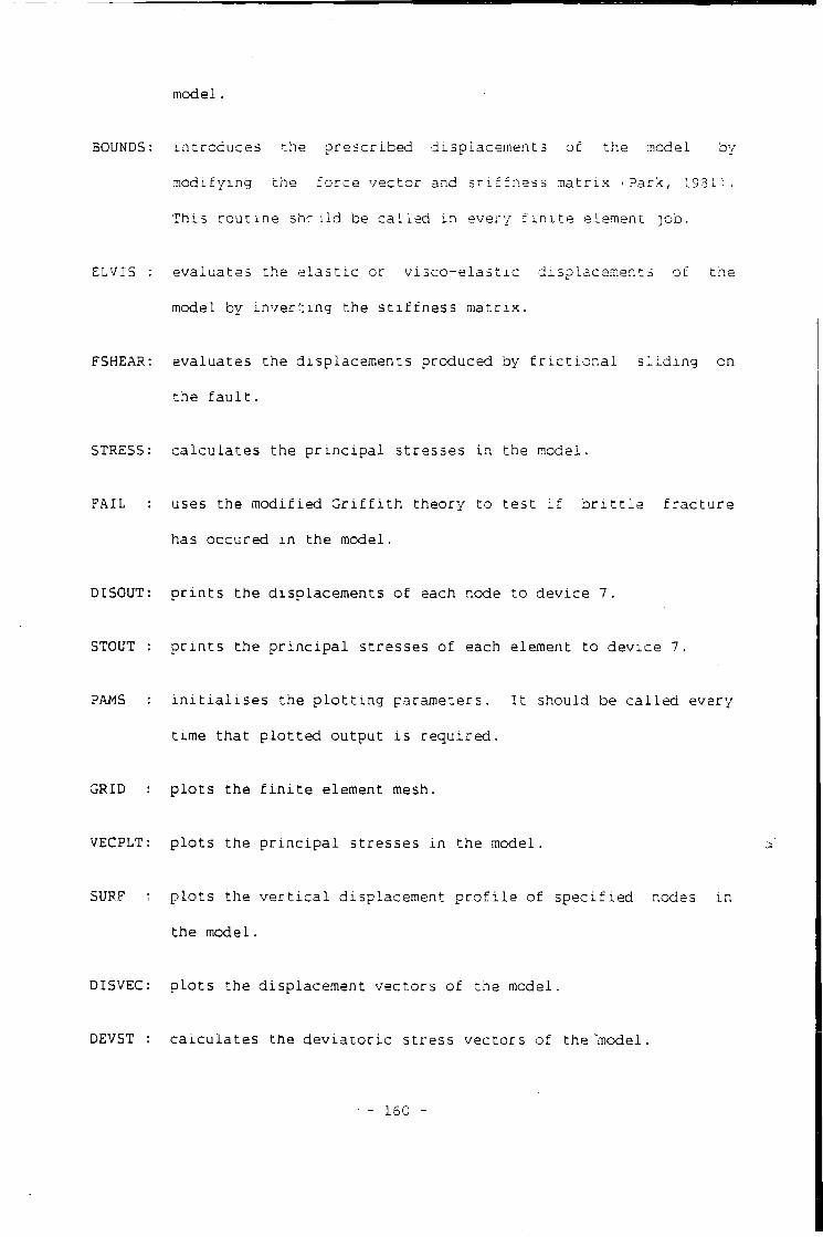
model.
BOUNDS: introduces the prescribed displacements of the model by
modifying the force vector and s t i f f n e s s matrix (Park, 1931';.
This r o u t i n e she ;Id be c a l l e d i n every f i n i t e element ]ob.
ELVIS : evaluates the e l a s t i c or v i s c o - e l a s t i c displacements of the
model by i n v e r t i n g the s t i f f n e s s m a t r i x .
FSHEAR: evaluates the displacements produced by f r i c t i o n a l s l i d i n g on
the f a u l t .
STRESS: c a l c u l a t e s the p r i n c i p a l stresses i n the model.
FAIL : uses the modified G r i f f i t h theory t o t e s t i f b r i t t l e f r a c t u r e
has occured i n the model.
DISOUT: p r i n t s the displacements of each node to device 7.
STOUT : p r i n t s the p r i n c i p a l stresses of each element t o device 7.
PAMS : i n i t i a l i s e s the p l o t t i n g parameters. I t should be c a l l e d every
time t h a t p l o t t e d output i s r e q u i r e d .
GRID : p l o t s the f i n i t e element mesh.
VECPLT: p l o t s the p r i n c i p a l stresses i n the model.
SURF : p l o t s the v e r t i c a l displacement p r o f i l e of s p e c i f i e d nodes i n
the model.
DISVEC: p l o t s the displacement vectors of the model.
DEVST : c a l c u l a t e s the d e v i a t o r i c stress vectors of the "model.
- 160 -
A . 2 . 2 E x ternal subroutines
Three e x t e r n a l subroutine l i b r a r i e s are i n t e r n a l l y referenced i n
ISOLIB. The f i r s t i s the MTS system subroutine TIME which evaluates the
CPU time which elapses between s p e c i f i e d i n s t r u c t i o n s . The second i s the
*HARWELL subroutine MA07BD which i n v e r t s a banded c o e f f i c i e n t m a t r i x . The
t h i r d i s the *GHOST p l o t t i n g system. There are numerous c a l l s to r o u t i n e s
i n t h i s l i b r a r y (e.g. FRAME and GREND) .
A . 3 ISOFELP: The Construction Of A C a l l i n g Sequence
ISOFELP (.isoparametric F i n i t e ELement Package) i s the main FORTRAN
w r i t t e n programming segment. This program contains a c a l l to each of the
f i n i t e element subroutines which have been described i n sec t i o n A . 2 . 1 . In
most f i n i t e element jobs i t w i l l not be desired to c a l l a l l of the
a v a i l a b l e subroutines. The user must t h e r e f o r e d e f i n e those modules which
are not t o be c a l l e d by i n s e r t i n g a C i n the f i r s t column of the r e l e v a n t
l i n e ( s ) . This has the e f f e c t of making the c a l l a comment, which i s
non-executable d u r i n g running of the program.
This approach t h e r e f o r e provides the user w i t h a set of subroutines
which can be used t o model a wide range of problems simply by modifying the
subroutines which are c a l l e d .
A.4 U t i l i s a t i o n
Once the user has modified ISOFELP there are two f u r t h e r steps t o
complete. The f i r s t i s to generate a set of input data which describes the
geometry, p h y s i c a l p r o p e r t i e s and boundary c o n d i t i o n s of the model. The
second step i s to l i n k and run the programs. These two steps are
- 1 6 1 -
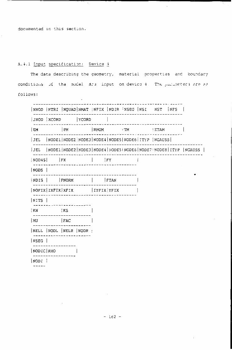
documented i n t h i s s e c t i o n .
A.4.1 Input s p e c i f i c a t i o n : Device 4
The data d e s c r i b i n g the geometry, m a t e r i a l p r o p e r t i e s and boundary
c o n d i t i o n s J £ the model a~ra i n p u t on device 4. The _u._:vieter s ere ??
f o l l o w s :
NNOD NTRI |NQUAD|NMAT NFIX |NDIR NSEG NSI NST |NFS 1 JNOD XCORD |YCORD 1 EM | PM RHOM TM ETAM |
JEL NODEl|NODE2|NODE3 NODE4|N0DE5 NODE6 ITYP NGALJSS |
JEL NODEl|NODE2|NODE3 NODE4!NODE5 NODES NODE7 NODE8|lTYP INGAUSS
N0D4S 1 FX i FY
NODS
NDIS IFNORM | FTAN
NOFIX IXFIX|XFIX IYFIX|YFIX
NITS
KN I K S
MU | F A C
NELL NODL |NELR |NODR
NSEG
NODIC RHO |
NODI
- 162 -
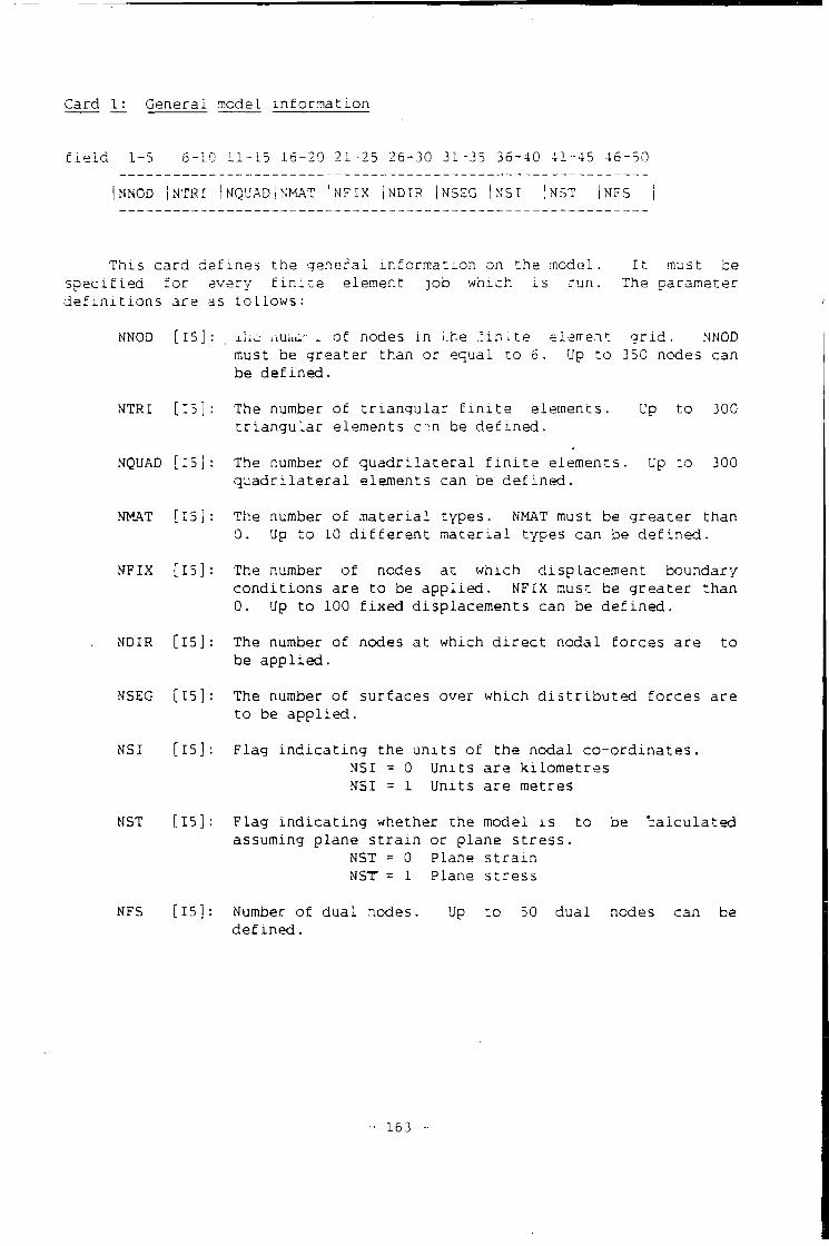
Card 1: General model i n f o r m a t i o n
f i e l d 1 - 5 6 - 1 0 1 1 - 1 5 1 6 - 2 0 2 1 - 2 5 2 6 - 3 0 3 1 - 3 5 3 6 - 4 0 4 1 - 4 5 4 6 - 5 0
NNOD IMTRI iNQUADlMMAT 'NFIX |NDIR | NSEG |NSI |NST |NFS \
This card defines the general i n f o r m a t i o n on the model. I t must be s p e c i f i e d f o r every f i n i t e element job which i s run. The parameter d e f i n i t i o n s are as f o l l o w s :
NNOD [15] : . of nodes i n i.he .:in.L.te elerrent g r i d . NNOD must be greater than or equal to 6 . Up t o 350 nodes can be d e f i n e d .
NTRI [ 1 5 ] : The number of t r i a n g u l a r f i n i t e elements. Up to 300 t r i a n g u l a r elements c.n be de f i n e d .
NQUAD [ 1 5 ] : The number of q u a d r i l a t e r a l f i n i t e elements. Up to 300 q u a d r i l a t e r a l elements can be d e f i n e d .
NMAT [ 1 5 ] : The number of m a t e r i a l types. NMAT must be greater than 0. Up t o 10 d i f f e r e n t m a t e r i a l types can be d e f i n e d .
NFIX [ 1 5 ] : The number of nodes at which displacement boundary c o n d i t i o n s are t o be ap p l i e d . NFIX must be greater than 0. Up to 100 f i x e d displacements can be d e f i n e d .
NDIR [ 1 5 ] : The number of nodes at which d i r e c t nodal forces are to be a p p l i e d .
NSEG [ 1 5 ] : The number of surfaces over which d i s t r i b u t e d forces are to be a p p l i e d .
NSI [ 1 5 ] : Flag i n d i c a t i n g the u n i t s of the nodal co-ordinates. NSI = 0 Units are ki l o m e t r e s NSI = 1 Units are metres
NST [ 1 5 ] : Flag i n d i c a t i n g whether the model i s to be c a l c u l a t e d assuming plane s t r a i n or plane s t r e s s .
NST = 0 Plane s t r a i n NST = 1 Plane s t r e s s
NFS [ 1 5 ] : Number of dual nodes. Up to 50 dual nodes can be de f i n e d .
- 1 6 3 -
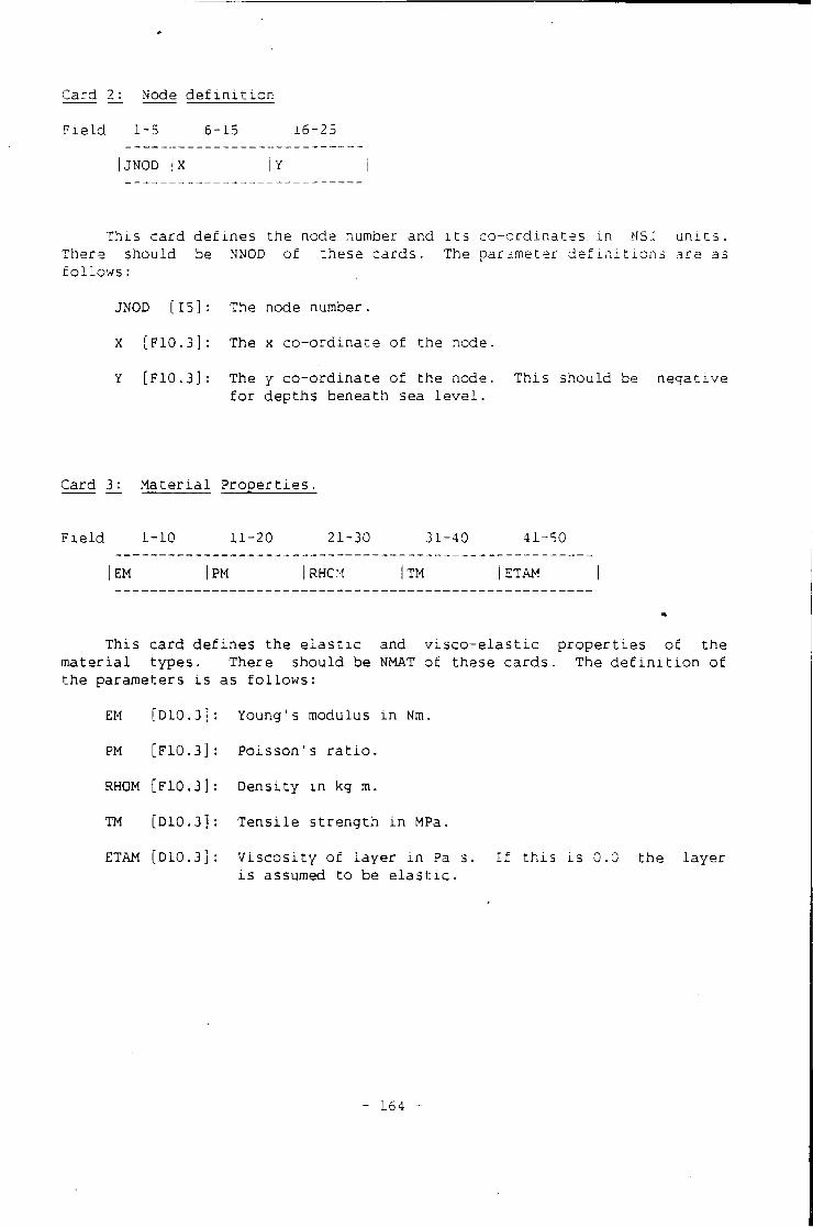
Card 2: Node d e f i n i t i o n
F i e l d 1-5 6-15
i JNOD IX
16-25
This card defines the node number and i t s co-ordinates i n NSI u n i t s , There should be NNOD of these cards. The parameter d e f i n i t i o n s are as f o l l o w s :
JNOD [ 1 5 ] : The node number.
X [F10.3]: The x co-ordinate of the node.
Y [F10.3]: The y co-ordinate of the node. This should be negative f o r depths beneath sea l e v e l .
Card 3: M a t e r i a l P r o p e r t i e s .
F i e l d 1-10
I EM 11-20 21-30 31-40 41-50
P M I R H C M I T M I E T A M
This card defines the e l a s t i c and v i s c o - e l a s t i c p r o p e r t i e s of the ma t e r i a l types. There should be NMAT of these cards. The d e f i n i t i o n of the parameters i s as f o l l o w s :
EM [D10.3]
PM [F10.3]
RHOM [F10.3]
TM [D10.3]
ETAM [D10.3]
Young's modulus i n Nm.
Poisson's r a t i o .
Density i n kg m.
Tensile s t r e n g t h i n MPa.
V i s c o s i t y of layer i n Pa s, i s assumed to be e l a s t i c .
I f t h i s i s 0.0 the layer
- 164 -
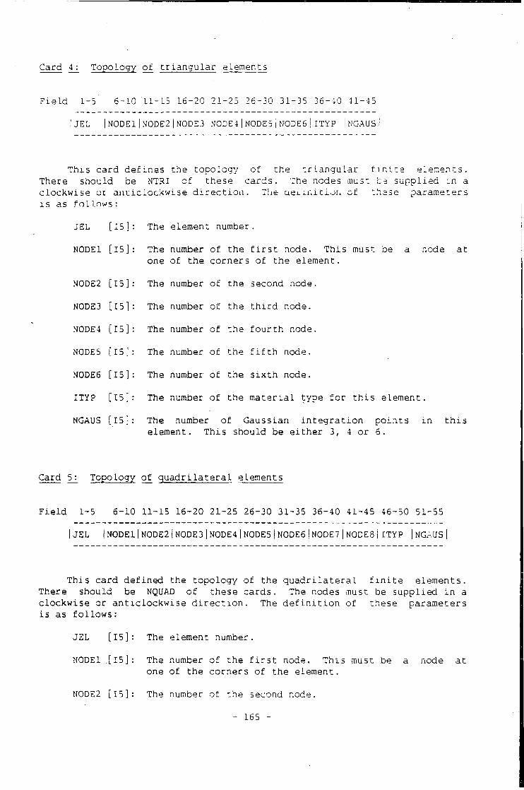
Card 4: Topology of t r i a n g u l a r elements
F i e l d 1-5' 6 - 1 0 1 1 - 1 5 1 6 - 2 0 2 1 - 2 5 2 6 - 3 0 3 1 - 3 5 3 6 - 4 0 4 1 - 4 5
|JEL I N 0 D E 1 I N 0 D E 2 ! N 0 D E 3 j N 0 D E 4 I N 0 D E 5 I K 0 D E 6 I I T Y P |NGAUS|
This card defines the topology of the t r i a n g u l a r f i n i t e elements. There should be NTRI of these cards. The nodes must ca supplied i n a clockwise or a n t i c l o c k w i s e d i r e c t i o n . The a e i m i t i o n of these parameters i s as f o l l o w s ;
JEL [ 1 5 ] : The element number .
N0DE1 [ 1 5 ] : The one
number of the
of the f i r s t node. This must be a node at corners of the element.
N0DE2 [ 1 5 ] : The number of the second node.
N0DE3 [ 1 5 ] : The number of the t h i r d node.
NODE 4 [ 1 5 ] : The number of the f o u r t h node.
NODES [15] : The number of the f i f t h node.
NODE 6 [ 1 5 ] : The number of the s i x t h node.
ITYP [ 1 5 ] : The number of the m a t e r i a l type f o r t h i s element.
NGAUS [ 1 5 ] : The number of Gaussian i n t e g r a t i o n p o i n t s i n t h i s element. This should be e i t h e r 3, 4 or 6.
Card 5: Topology of q u a d r i l a t e r a l elements
F i e l d 1-5 6-10 11-15 16-20 21-25 26-30 31-35 36-40 41-45 46-50 51-55
IJEL IN0DE1IN0DE2|N0DE3|NODE4|N0DE5|NODE6|N0DE7|NODE8|ITYP |NGAUS|
This card defined the topology of the q u a d r i l a t e r a l f i n i t e elements. There should be NQUAD of these cards. The nodes must be supplied i n a clockwise or a n t i c l o c k w i s e d i r e c t i o n . The d e f i n i t i o n of these parameters i s as f o l l o w s :
JEL [ 1 5 ] : The element number.
NODE1 [ 1 5 ] : The number of the f i r s t node. This must be a node at one of the corners of the element.
NODE2 [ 1 5 ] : The number of the second node.
- 1 6 5 -
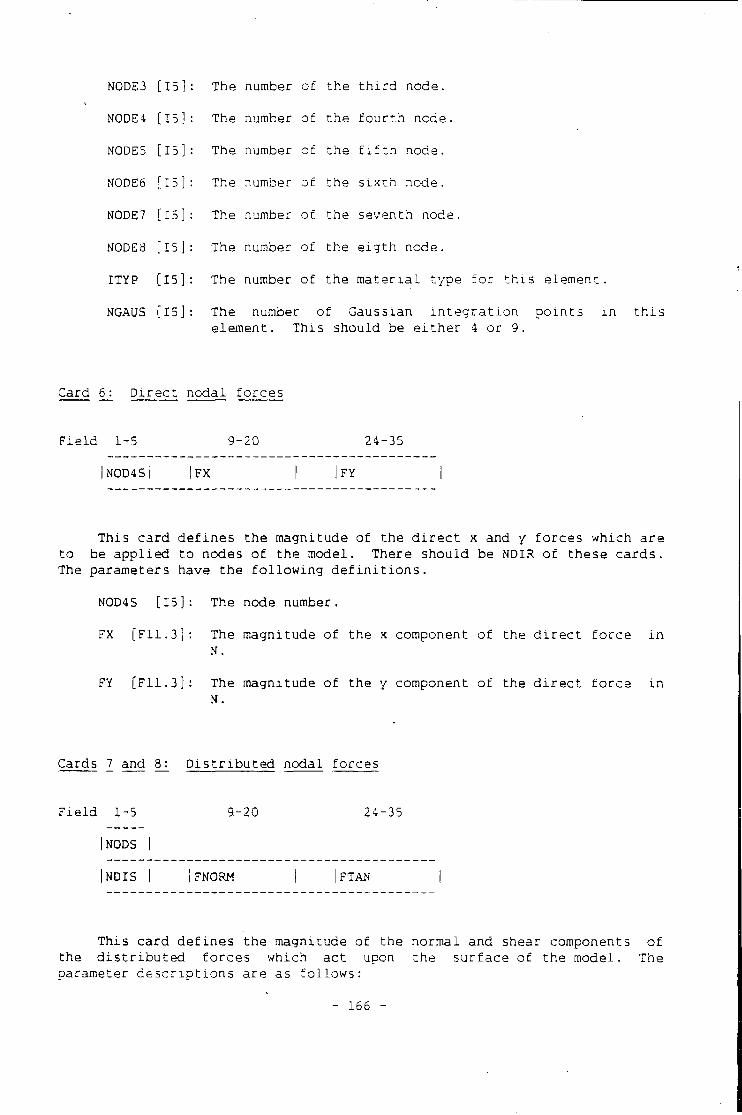
1 5 ] : The number of the t h i r d node.
1 5 ] : The number of the f o u r t h node.
1 5 ] : The number of the f i f t h node.
1 5 ] : The number of the s i x t h node.
1 5 ] : The number of the seventh node.
1 5 ] : The number of the e i g t h node.
1 5 ] : The number of the m a t e r i a l type f o r t h i s element.
1 5 ] : The number of Gaussian i n t e g r a t i o n p o i n t s i n t h i s element. This should be e i t h e r 4 or 9.
Card 6: D i r e c t nodal forces
F i e l d 1-5 9 - 2 0 2 4 - 3 5
|N0D4S| I FX I I FY |
This card defines the magnitude of the d i r e c t x and y forces which are to be app l i e d t o nodes of the model. There should be NDIR of these cards. The parameters have the f o l l o w i n g d e f i n i t i o n s .
N0D4S [ 1 5 ] : The node number.
FX [F11.3]: The magnitude of the x component of the d i r e c t f o r c e i n N.
FY [F11.3]: The magnitude of the y component of the d i r e c t f o r c e i n N.
Cards 7 and 8: D i s t r i b u t e d nodal forces
F i e l d 1-5 9 - 2 0 24-35
I NODS |
I N D I S I IFNORM I |FTAN |
This card d e f i n e s the magnitude of the normal and shear components of the d i s t r i b u t e d forces which act upon the surface of the model. The parameter d e s c r i p t i o n s are as f o l l o w s :
N0DE3
NODE 4
N0DE5
N0DE6
N0DE7
NODES
ITYP
NGAUS
- 1 6 6 -
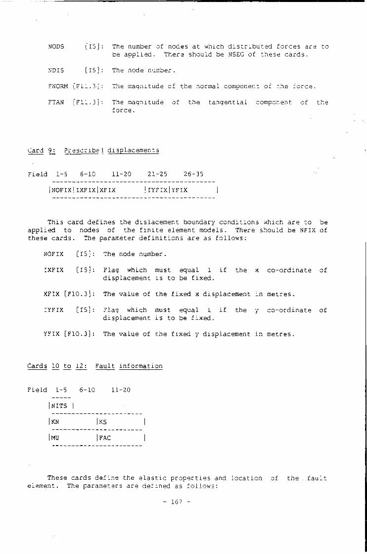
MODS [ 1 5 ] : The number of nodes at which d i s t r i b u t e d forces are to be a p p l i e d . There should be NSEG of these cards.
NDIS [ 1 5 ] : The node number.
FNORM [F11.3]: .The magnitude of the normal component of the f o r c e .
FTAN [F11.3]: The magnitude of the t a n g e n t i a l component of the fo r c e .
Card 9: Prescribed displacements
F i e l d 1-5 6-10 11-20 21-25 26-35
NOFIXlIXFIX|XFIX | I Y F I X | Y F I X
This card defines the dislacement boundary c o n d i t i o n s which are to be ap p l i e d to nodes of the f i n i t e element models. There should be N F I X of these cards. The parameter d e f i n i t i o n s are as f o l l o w s :
NOFIX
IXFIX
[15]
[15]
XFIX [F10.3]
IYFIX [15]
The node number.
Flag which must equal 1 i f the x co-ordinate of displacement i s t o be f i x e d .
The value of the f i x e d x displacement i n metres.
Flag which must equal 1 i f the y co-ordinate of displacement i s to be f i x e d .
YFIX [F10.3]: The value of the f i x e d y displacement i n metres
Cards 10 t o 12: Fault i n f o r m a t i o n
1-5 6-10 11-20
N I T S
KN I K S
MU |FAC
These cards d e f i n e the e l a s t i c p r o p e r t i e s and l o c a t i o n of the . f a u l t element. The parameters are de f i n e d as f o l l o w s :
- 167 -
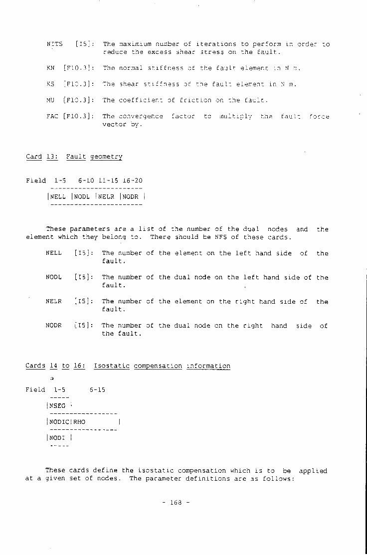
NITS [ 1 5 ] : The maximium number of i t e r a t i o n s to perform i n order t o reduce the excess shear stress on the f a u l t .
KN [F10.3]: The normal s t i f f n e s s of the f a u l t element i n N m.
KS [F10.3]: The shear s t i f f n e s s of the f a u l t element i n N m.
MU [F10.3]: The c o e f f i c i e n t of f r i c t i o n on the f a u l t .
FAC [F10.3]: The convergence f a c t o r to m u l t i p l y the f a u l t f o r c e vector bv.
Card 13: Fault geometry
F i e l d 1-5 6-10 11-15 16-20
I NELL INODL INELR |NODR I
These parameters are a l i s t of the number of the dual nodes and the element which they belong t o . There should be NFS of these cards.
NELL [ 1 5 ] : The number of the element on the l e f t hand side of the f a u l t .
NODL [ 1 5 ] : The number of the dual node on the l e f t hand side of the f a u l t .
NELR [ 1 5 ] : The number of the element on the r i g h t hand side of the f a u l t .
NODR [ 1 5 ] : The number of the dual node on the r i g h t hand side of the f a u l t .
Cards 14 to 16: I s o s t a t i c compensation i n f o r m a t i o n
F i e l d 1-5 6-15
NSEG |
NODICIRHO
NODI
These cards d e f i n e the i s o s t a t i c compensation which i s t o be a p p l i e d at a given set of nodes. The parameter d e f i n i t i o n s are as f o l l o w s :
- 1 6 3 -
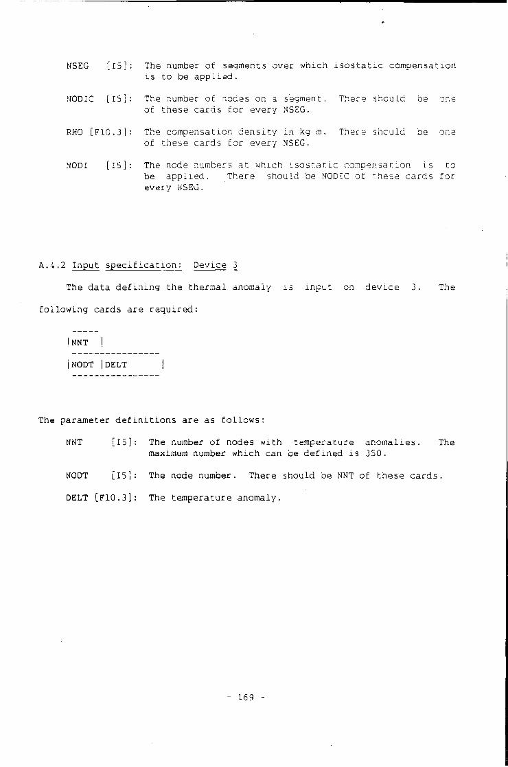
NSEG [ l b ] : The number of segments over which i s o s t a t i c compensation i s to be a p p l i e d .
NODIC [ 1 5 ] : The number of nodes on a segment. There should be one of these cards f o r every NSEG.
RHO [F10.3]: The compensation d e n s i t y i n kg m. There should be one of these cards f o r every NSEG.
NODI [ 1 5 ] : The node numbers at which i s o s t a t i c compensation i s to be a p p l i e d . There should be NODIC of these cards f o r every NSEG.
A.4.2 Input s p e c i f i c a t i o n : Device 3
The data d e f i n i n g the thermal anomaly i s i n p u t on device 3. The
f o l l o w i n g cards are re q u i r e d :
| NNT !
INODT IDELT I
The parameter d e f i n i t i o n s are as f o l l o w s :
NNT [ 1 5 ] : The number of nodes w i t h temperature anomalies. The maximum number which can be defined i s 350.
NODT [ 1 5 ] : The node number. There should be NNT of these cards.
DELT [F10.3]: The temperature anomaly.
- 1 6 9 -
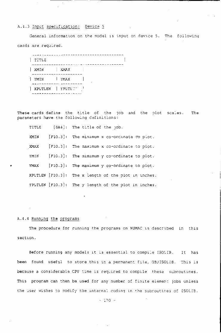
A.4.3 Input s p e c i f i c a t i o n : Device 5
General i n f o r m a t i o n on the model i s i n p u t on device 5. The f o l l o w i n g
cards are req u i r e d .
TITLE
XMIN I XMAX
YMIN 1 YMAX
XPLTLEN I YPLTL":"
These cards d e f i n e the t i t l e of the job and the p l o t scales parameters have the f o l l o w i n g d e f i n i t i o n s :
The
TITLE
XMIN
XMAX
YMIN
YMAX
[8A4]
[F10.3]
[F10.3]
[F10.3]
[F10.3]
XPLTLEN [F10.3]
YPLTLEN [F10.3]
The t i t l e of the job.
The minimum x co-ordinate Do p l o t .
The maximum x co-ordinate to p l o t .
The mimimum y co-ordinate to p l o t .
The maximum y co-ordinate to p l o t .
The x length of the p l o t i n inches.
The y length of the p l o t i n inches.
A.4.4 Running the programs
The procedure f o r running the programs on NUMAC i s described i n t h i s
s e c t i o n .
Before running any models i t i s e s s e n t i a l to compile ISOLIB. I t has
been found u s e f u l to st o r e t h i s i n a permanent f i l e , OBJISOLIB. This i s
because a considerable CPU time i s r e q u i r e d to compile these s u b r o u t i n e s .
This program can then be used f o r any number of f i n i t e element jobs unless
the user wishes to modify the i n t e r n a l coding i n the subroutines of ISOLIB.
- 1 7 0 -
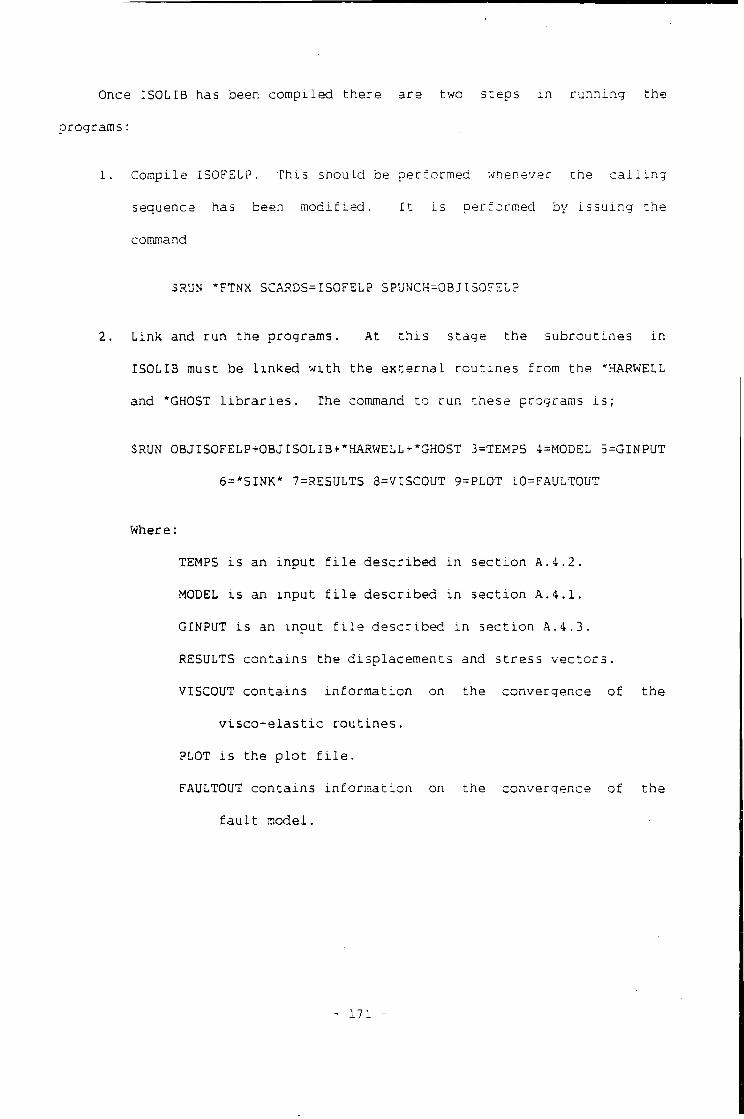
Once ISOLIB has been compiled there are two steps i n running the
programs:
1. Compile ISOFELP. This should be performed whenever the c a l l i n g
sequence has been modified. I t i s performed by i s s u i n g the
command
$RUN *FTNX SCARDS=ISOFEL? SPUNCH=OBJISOFEL?
2. Link and run the programs. At t h i s stage the subroutines i n
ISOLIB must be l i n k e d w i t h the e x t e r n a l r o u t i n e s from the "HARWELL
and *GHOST l i b r a r i e s . The command to run these programs i s ;
$RUN OBJISOFELP+OBJISOLIB+'HARWELL+'GHOST 3=TEMPS 4=M0DEL 5=GINPUT
6=*SINK* 7=RESULTS 8=VISC0UT 9=PL0T 1OFAULT0UT
Where:
TEMPS i s an in p u t f i l e described i n s e c t i o n A.4.2.
MODEL i s an inp u t f i l e described i n se c t i o n A.4.1.
GINPUT i s an input f i l e described i n s e c t i o n A.4.3.
RESULTS contains the displacements and stress v e c t o r s .
VISCOUT contains i n f o r m a t i o n on the convergence of the
v i s c o - e l a s t i c r o u t i n e s .
PLOT i s the p l o t f i l e .
FAULTOUT contains i n f o r m a t i o n on the convergence of the
f a u l t model.
- 171 -

A.5 Program L i s t i n g s
- 1 7 2
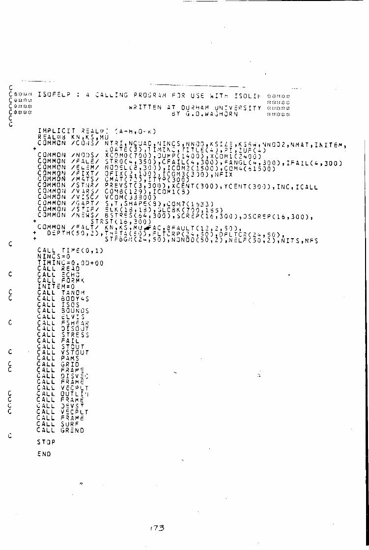
c c
c c
ISOFELP A CALLING PROGRAM FOR USE *ITh ISOLIe WRITTEN AT DURHAM UNIVERSITY
SY G.Q.WAGHORN
I M P L I C I T REAL R E A L * 3 K N , K S , M U C O M M O N / C Q• J5/
:A-h,o-w)
C O M M O N C O M M O N C O M M O N C O M M O N C O M M O N C O M M O N C O M M O N C O M M O N C O M M O N C O M M O N C O M M O N
C O M M O N
/NODS/ /rALE/ /E L EM/ / F I X T / /MATS/ / S T N R / / V A R S/ /VISC/ / G A P T / /S TIF/ /NEWS/
ST /FALT/
D£PTH(5 0,2)
N T R I , N C U A Q , N I N C S , N N a O , H S I Z = i K 5 B w , N N a 0 2 i N M A T | I N I T g M » iOATt(3> ,1 I M I N C , T I T L E ( 4 j , ? I , I U F U ) XCOM0(7OO),-IUNP(l<t00),XCQMl(2tQ0) S T R O ( < , , 3 5 0 ) , C F A I L ( < M 3 0 0 ) , F A N G L ( < » , 3 0 0 ) , I F A I L U , 3 0 0 ) N Q D E L C 3 , 3 0 0 ) , I C O M 2 C 1 5 0 Q ) . C C M 4 C 6 1 5 0 0 )
TY»C300) i300),XCENTC300),YCENT(30 0 ) , I N C F I C A L L PREVSTC3
CQM3C129),IC0M1C5) VCQMCJ3300) S,T,SHAPEC3),C0M7(153 3 ) ELKC18 ,13),GLC3K(700,1S5) 6STRES(64,300),SCR£PC16,300 ),OSCREP<:i6,300), RSU 16 . 200 ) KN,KS,WU^FAC,8PAULT(12,2.5 0 ) , ,TnETA(5 0),PLTCRPC2^,50),OFLTCRC2 STroGN(2<-,50), NONO0C50, 2) ,N~ . - » 50) ,
L F ( 5 0 , 2 ) , N I T S , N F S
C A L L T I M E C O , 1) N I N C S = 0 T I M I N C = 0 . O D + 0 0 C A L L R E A D C A L L E C H O C A L L F O R M * INITEM=0 C A L L T A N Q M C A L L 6 0 D Y 4 S C A L L I S O S C A L L 3 0 U N D S C A L L ( E L V I S C A L L F S M E A R C A L L O I S O U T C A L L S T R E S S C A L L F A I L C A L L S T O U T C A L L V S T 0 U T C A L L P A M S C A L L G R I D C A L L F R A M E C A L L Q I S V E C C A L L F R A M E C A L L V E C P L T C A L L O U T L I ' I C A L L F R A M E C A L L 3 E V S T
C A L L V E C P L T C A L L F R A M E C A L L S U R F C A L L G R E N O
S T O P
E N D
173
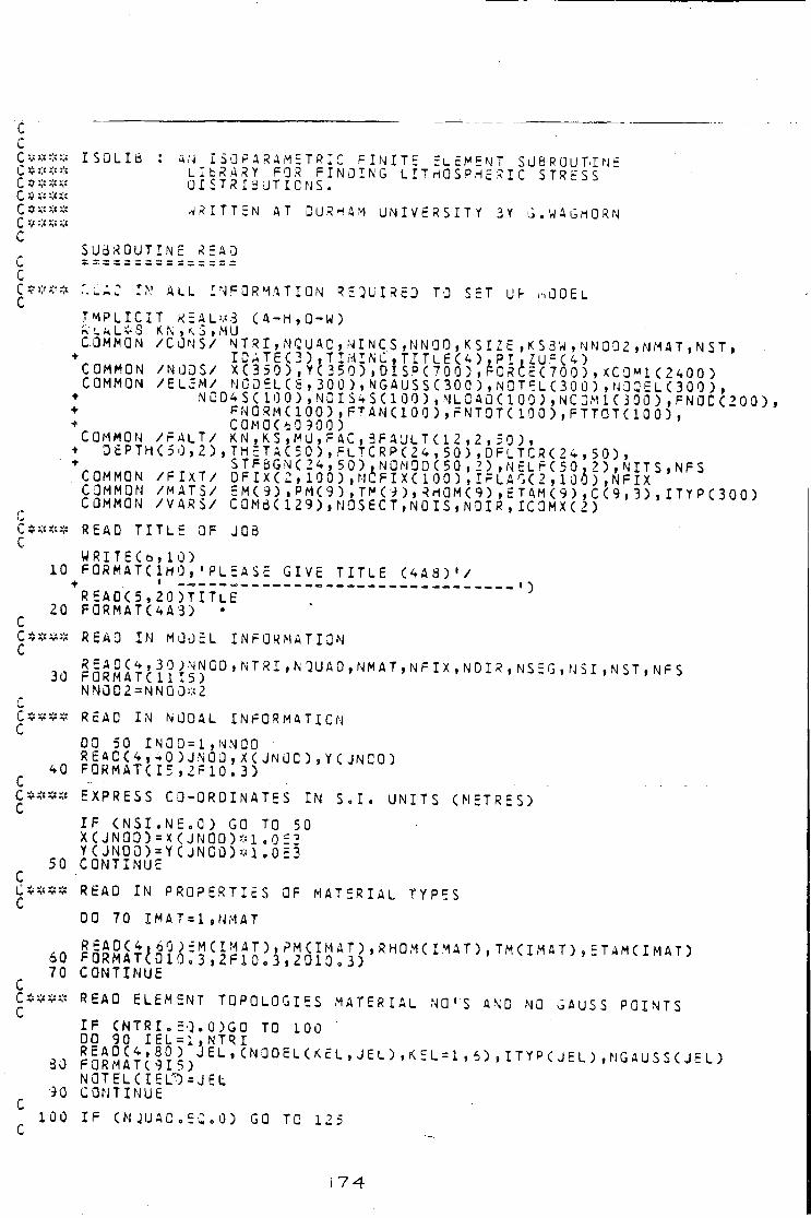
SUBROUTINE SEAO
C***:;; ISOLIB : A N ISOPARAMETRIC F I N I T E E L E M E N T S J B R O U T . T N P J-**** LlbRARY F O R F I N O I N G LITriOSPHERIC S T R E S S C * ? f * OISTRI3UTICNS. j r * * * * W R I T T E N A T D U R H A M UNIVERSITY 3Y G . W A G H Q R N
C :r *>J *«: -JS
c c c C P * I M A L L I N F O R M A T I O N R E Q U I R E D T O S E T ut- C , O O E L
I M P L I C I T REALMS (A-HtQ-W) ^LkL*3 K N , K . 3 , M U COMMON /CONS/ NTRI,NCUAC,NINCS ,NNOO,KSIZE , K S 8W , NN 002 , NM A T . N S T ,
• I 0 A T E C 2 ) , T I M I N C , T I T L E C 4 ) , P I .ZUF(0 COMMON /NODS/ XC 3 50 ) , YC 350) , 0 I SP( 700 ) ,F0RtEC 700),X C0M1(2 *00) COMMON / E L E M / NGDEL(6 , 300),NGAUSS(300),NOTELC300),NOQFLC300),
+ NCQ4SC10 0),NGIS*S(100),NLCAO(10Q),NC3M1(JOO),FNOCC200), • pNORMC100),FTANC100)irNTOTC100),FTTOT(100), + CQMOC60900) COMMON /FALT/ K N , K S , MU,FAC,3FAULT (12,2,50), • OtPTHC5 0,2),THETAC50),FLTCRP<24,50),OFLTCRC24,50), , STFSGNC24,50),NONODC50,2) , N E L F < 5 0 . 2 ) , N I T S , NF S COMMON /FIXT/ D F I X ( 2 , 1 0 0 ) , M C F I X C 1 0 0 ) , I r L AG ( 2 , 1 0 5 ) , N F I X COMMON /MATS/ EM(9),PM(9),TMC9),RdaM<9),ETAMC9),CC9,3),ITYPC300) COMMON /VARS/ C0M6<129),N0S6CT,N0IS,N0IR,IC0MXC2) C*f« READ TITLE OF JOB C
WRITECotlO) 10 FORMATC1H0,'PLEASE GIVE TITLE ( 4 A 8 ) ' /
R EAO(5,20)TITLE~~ ' 5
20 FGRMATC4A3) C * # * « READ IN MODEL INFORMATION
30 F Q R M A T < 1 1 I 5 ) G D , N T R I ' N Q U A 0 • N M A T » N F 1 X • N ' 0 1 R ' N ^ E G , N S I , N S T , N F S NNGD2=NNOD*2
C C***s READ IN NODAL INFORMATION
00 50 IN00=1,NN00 REACC4,40)JN00,X(:JN0C),Y<JNC0)
40 F0RMATCI5 ,2F10.3) C***3 EXPRESS CO-ORDINATES IN S.I. UNITS (METRES)
IF CNSI.NE .O) GO TO 50 X(JNOO )=X<JNOO)*1 „0E2 Y <JNOD ) = Y (JNG0)*1.0E3 50 CONTINUE
C
C***s READ IN PROPERTIES OF MATERIAL TYPES DO 70 IMAT=1jNMAT
60 n^ikin^^^ 70 CONTINUE
C C**3* READ ELEMENT TOPOLOGIES MATERIAL NO 'S AND NO GAUSS POINTS
IF (NTRIoEO.O)GO TO 100 DO 90 IEL=1,NTRI
30 F a R M A T C 9 I 5 ) J E t " C N 0 0 E L U £ L ' J £ L ) > * E L = 1 > ^ »ITYP(JEL ) , N G A US S C J E L )
NGTELC IEL^) = JEL 90 CONTINUE
100 IF (NJUACEw . O ) GO TO 125 c
1 7 4
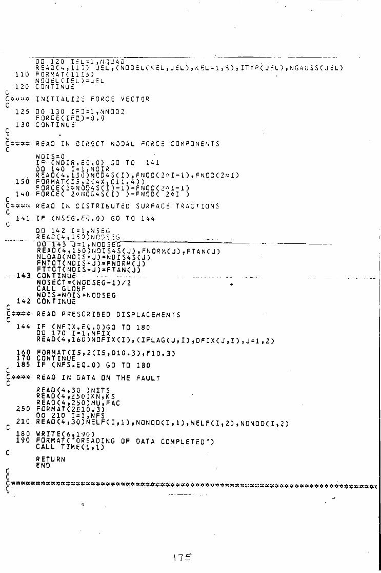
0 0 1 2 0 I E L = 1 , N - J U 4 0 R E A D ( T , 1 1 0 ) J £ L , C N 0 0 E L C K E L , J E L ) , K E L = 1 ) S ) , I T Y P ( J E L ) , N G A U S S ( J C L )
1 1 0 F 0 R M A T ( 1 1 I 5 ) N O U E L ( I E L ) = J E L
1 2 0 C O N T I N U E C C S ^ * * I N I T I A L I Z E F O R C E V E C T O R C
1 2 5 0 0 1 3 0 I F G = 1 , N N 0 0 2 F O R C 5 C I F C . ) = 0 . 0
1 3 0 C O N T I N U E ' C
CSitifZ R E A D I N O I R E C T N O D A L F O R C E C O M P O N E N T S C
N O I S = 0 IP' ( N O I R . E Q . O ) G O T O 1 4 1 00 1 4 0 I = 1 , N 0 I R R = A 0 ( 4 , 1 5 0 ) N C D 4 S ( I ) , F N 0 Q C 2 * I - 1 ) , F N 0 C ( 2 * I )
150 F 0 R M A T < I 5 , 2 C 4 X , C 1 1 . 4 ) ) F 0 R C E ( 2 * N 0 D 4 S ( I ) - 1 ) = F N 0 C ( 2 * 1 - 1 )
1 4 0 FORCEC 2 * N 0 0 4 $ ( I ) ) = F N G O C 2 * 1 ) C C*S** R E A D I N D I S T R I B U T E D S U R F A C E T R A C T I O N S C
1 4 1 I F CNSEG . E Q . O ) G O T O 1 4 4 C
D O 1 4 2 I = 1 , N S E G R EA. cJ_ 4il 5 0 ) N C Q vS G 00 143 J = l , NODSE~G READ(4,lbO)NDIS4SCJ),FNORM<J),FTANCJ) NL0ADCNOIS+J)=N0IS4S(J) FNTOT(NDIS+J)=FNORM(J) FTTOT(NOIS+J)=FTAN<J) — 1 * 3 - CONTINUE -N0SECT=(N00SEG=l)/2 CALL GLOBF NDIS=NOIS+NODSEG 142 CONTINUE
r C*$*« READ PRESCRIBED DISPLACEMENTS
144 I F CNFIX. EQ.OGO TO 1 8 0 00 170 I=1,NFIX READ(4,160)NOFIXCI),CIFLAGCJiI) iDFIXCJ, I ) , J = l ,2)
tfi C F O Q 5 ? ^ E l 5 , 2 C I 5 ' D 1 ° - 3 ) ' F 1 0 - 3 )
185 IF (NFS.EQ.O) GO TO 180 C***« R EAO IN DATA ON THE FAULT C
READC4 ,30 )NITS READ(4,250)KN,KS REA0C4,250)MU,FAC 250 FORMATC2E10.3) DO 210 I= 1,NFS
210 REAO<4,30)NELFCI,l),NONODCI,n,NELFCI,2),NQNODCI,2) 180 W R I T E < 6 , 1 9 0 ) 190 FORMATC'OREADING OF DATA COMPLETED') CALL TIMECl.l)
RETURN END C c
175
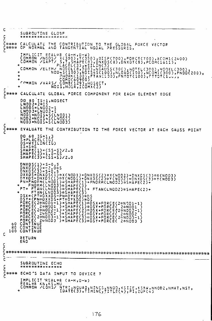
c : • SUBROUTINE GL03F C =================
c C$s*s CALCULATE THE CONTRIBUTION TO THE GLOBAL FORCE VECTOR C***s OF NORMAL AND TANGENTIAL NODAL PRESSURES.
IMPLICIT REAL#8 CA-H,0-W) COMMON /NODS/ X(350) , YC350 ) , DISPC700) , FORCE<700) , XC0M1(2400 ) COMMON /GAPT/ S,T,SHAPEC8),DNXDSC8) , DNXDT(8) , PCOMC1611 ) ,
+ - PLACELC3).WEILINC3) COMMON /EL EM/ NQDELC8i300)tNGAUSSC30C),NOTF.LC300)fNOQELC30O)i + NOD^S(100),NDIS4S(1005,NLOADC100),NCOMl(3O0),FNODC200) • PNORKC130) I F T A M C I O O ) I F N T O T C I O O ) iTTTOTCl-wwy , + CQMOC60900) r n MMON /VASS/ COMBC129).NGScCT,
• NOISiNOIRfICQMXC2) C*#S* CALCUL ATh GLOBAL FORCE COMPONENT FOR EACH ELEMENT EDGE
DO 80 'lS = l .NOSECT LN0D2=2*IS LN0D1=LN0D2-1 LNOQ3=LNOD2+1 N0D1=N0IS4SCLN0D1) N002=NDIS4SCLN0D2 ) N0D3=NDIS4SCLN0D3)
C C*«** EVALUATE THE CONTRIBUTION TO THE FORCE VECTOR AT EACH GAUSS POINT
DO 60 IG=1,3 S=PLACELCIG) OS=WEILINCIG) s S=S SS SHAPfECl) = CSS-S)/2.0 SHAPEC2)=1.0-SS SHAPEC3)=CSS+S)/2.0 DNX0SCl)=S-0.5 DNXOSC2)=-2.0*S DNXDSC3)=S+0.5 DXXDS = 0NXDSC1)*XCN0D1)+DNXDSC2)*XCN0D2)+0NXCS C3)*XCN00 3) DYXOS=DNXDSCl)*YCNODl)+DNXDSC2)*YCNaD2)+ONXDSC3)*YCNOD3) PN = FN0PMCLN0D1)*SHAP5C1) +FNORMCLN002)*SHA PEC 2) + • FNQRM(LN0D3)*SHAPEC3) PT= FTAN(LN0D1)#SHAPEC1)+ FT ANCLNQD2)*SHAPEC2) + • FTAN(LN0D3)*SHAPEC3) DSX=CPT*DXXDS-PN*DYXDS)*OS DSY=CPN*OXXDS+PT*OYXDS)#OS F0RCEC2SN0D1-1)=SHAPEC1)*0SX+F0RCEC2*NQD1-1) FORCEC 2*NQD1 )=SHAPEC1)*DSY+F0RCEC 2*N0D1 ) FORCEC 2*N0D2-1) = SHAPEC2OS X+ F0RCEC2SN0D2-1) FORCEC 2*NCD2 )=SHAPEC2)*0SY + FORC5C 2SN002 ) FORCEC 2*N0D3-1)=SHAPEC3)*0SX+F0RCEC2*N003-1) FORCEC 2*N0D3 )=SHAPEC3)*DSY +FORCEC 2*N0D3 ) 60 CONTINUE 80 CONTINUE 100 CONTINUE C RETURN END C C
C " • • SUBROUTINE ECHO
C 3 S S S 3 3 3 3 = = = = S = = c C#*3* ECHO'S DATA INPUT TO OEVICE 7
IMPLICIT T?5AL*8 CA-H.O-W) R EAL*8 KN,KS,MU COMMON /CONS/ NTRI,NQUAD,NINCS,NNaD,KSi:E,KSRW,NNQD2,NMAT,NST. + IDATEC3),TIMINC,TITLEC4),PI SZUFC4)
176
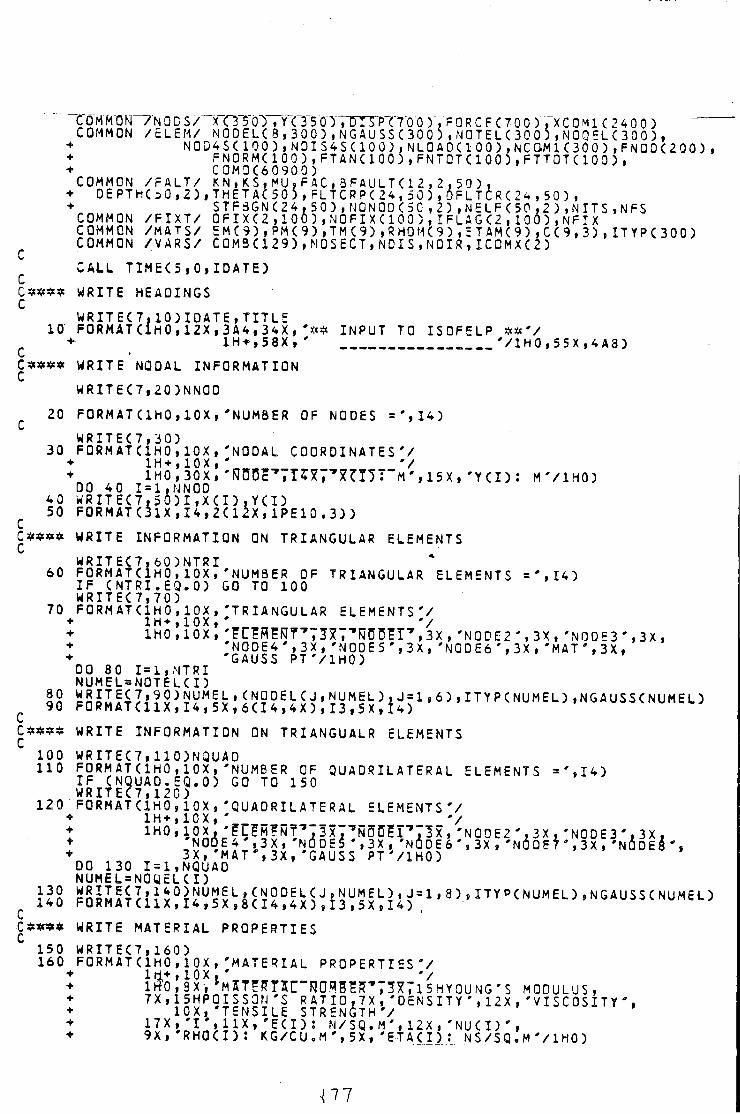
C O M M O N / N O D S / X OTO") . Y C3"5"0" TDTSlPT7 0 0 ) ' . PQ R C F. ( 7 0 0 ) T X C O M 1 C 2 4 0 0 ) C O M M O N / E L E M / N 0 D E L ( 8 , 3 0 0 ) , N G A U S S ( 3 0 0 5 , N 0 T E L < 3 0 0 ) , N 0 Q E L ( 3 0 0 ) ,
+ N O D 4 S ( 1 0 0 ) , N D I S 4 S ( 1 0 0 ) , N L O A D ( 1 0 0 ) , N C Q - M 1 ( 3 0 0 ) , F N O 0 ( 2 0 0 ) , + F N O R M ( 1 0 0 ) , F T A N ( 1 0 0 ) , F N T O T ( 1 0 0 ) , F T T O T ( 1 0 0 ) , + C O M O ( 6 0 9 0 0 )
C O M M O N / F A L T / K N , K S , M U , F A C , 3 F A U L T ( 1 2 , 2 , 5 0 ) , • D E P T H ( 5 0 , 2 ) , T H E T A ( 5 0 ) , F L T C R P ( 2 4 , 5 0 ) , 6 F L T C R ( 2 4 , 5 0 ) , + S T F 3 G N ( 2 4 . 5 0 ) , N O N O D ( 5 0 , 2 ) , N E L F ( 5 P , 2 ) , N I T S , N F S
C O M M O N / F I X T / 0 F I X ( 2 , 1 0 0 ) , N 0 F I X ( 1 0 0 ) , I F L A G ( 2 , 1 0 0 ) , N F I X C O M M O N / M A T S / E M ( 9 ) , P M ( 9 ) , T M ( 9 ) , R H O M ( 9 ) , E T A M ( 9 ) , C ( 9 , 3 ) , I T Y P ( 3 0 0 ) C O M M O N / V A R S / C O M B ( 1 2 9 ) , M O S E C T , N O I S , N D I R , I C O M X ( 2 )
CALL T I M E ( 5 , 0 , I D A T E ) C C * * * $ WRITE HEADINGS C
10 WRITE(7.10)IDATE,TITLE FORMAT(lH0,12X,3A4,34X,'** INPUT TO ISOFELP *#'/
+ 1H+,58X,' V1H0,55X,4A3) C**«* WRITE NODAL INFORMATION
WRITE(7,20)NN0D 20 FORMAT(lh0,10X,'NUMBER OF NODES = ' , I 4 )
W R I T E ( 7 , 3 0 ) 30 FORMAT(1HO,10X, 'NODAL COORDINATES'/
• 1H+.10X,' '/ + 1H0 , 30X . 'FJnnP"*TTI7T'77TTT~M ' DO 40 I=1.NN0D
40 W R I T E ( 7 . 5 0 ) I , X ( I ) , Y ( I ) 50 FORMAT(31X,I4,2(12X,1PE10.3))
1M+ , 1 0 X , '/ 1H0,30X, 'fIBBE" ,7TSx7" Fx7IT7~M' Ii5X, ' Y ( I ) : MVIHO)
c C * * * * WRITE INFORMATION ON TRIANGULAR ELEMENTS C
WRITE(7,60)NTRI 60 FORMATUHO,10X, 'NUMBER OF TRIANGULAR ELEMENTS = ' , I 4 ) IF (NTRI.EQ.O) GO TO 100 WRITE(7,70) 70 FORMATUHO , 10X , 'TRIANGULAR ELEMENTS'/ + 1H+,10X,' '/ 1H +, 10X , '/
1H0,10X, '?C?RFFIT"'T3"7T""FJ0C?T"', 3X , 'NODE 2 ' , 3X , 'NODE 3 ' , 3X , 'N0DE4',3X, 'N0DE5',3X, 'NQDE6',3X, 'MAT',3X, 'GAUSS PT'/IHO) DO 80 I=1,NTRI NUME L= NOT E L ( I ) IS H S n ! i J , » 9 0 j N U M E L » <NOOEL( J.NUMEL) , J = l ,6) ,ITYP(NUMEL) ,NGAUSS(NUMEL) 90 F0RMAT(11X,I4 I5X,6(I4,4X),I3,5X,I4)
C * « * * WRITE INFORMATION ON TRIANGUALR ELEMENTS 100 WRITE(7,110)NQUAD 110 FORMAT(1H0,10X, 'NUMBER OF QUADRILATERAL ELEMENTS = ' , I 4 ) IF (NQUAD.EQ.O) GO TO 150 WRITE(7,120) 120 FORMAT(1H0,10X, 'QUADRILATERAL ELEMENTS'/
• 1H+.1CX,' */ + iHO.iqx, ' f t E M f N T ^ ^ J ^ N ^ • 'NODE 4',3X, 'NODES *,3X, 'NODE 6',3X, 'N00E7',3X,'NODES', + ,„„ 3X, 'MAT',3X, 'GAUSS PT'/IHO) DO 130 I=1,NQUAD NUME L = NOQEL(I)
^ 140 FORMAT(11X,14,5X,8(14,4X),13 ,5X,14) C * * « * WRITE MATERIAL PROPERTIES
150 WRITE(7,160) 160 FQRMATUHO , 10X ,'MATERIAL PROPERTIES'/
• 1H +,10 X. ' ' / + l t t O i 9X-, *MlTETr5C~R0RBEff'73x7l5HY0UNG*S MODULUS, • 7X,15HP0ISS0N 'S RAT 10 , 7 X , * DENSITY',12X, ' V I SC0SITY + 10X, TENSILE STRENGTH'/ • 17X, 'I',11X, ' E ( I ) : N/SQ.M ' ,12X, ' N U ( I ) ' , • 9X,'RH0(I): KG/CU.M',5X, ' E T A ( I ) : NS/SQ.M'/IHO)
01
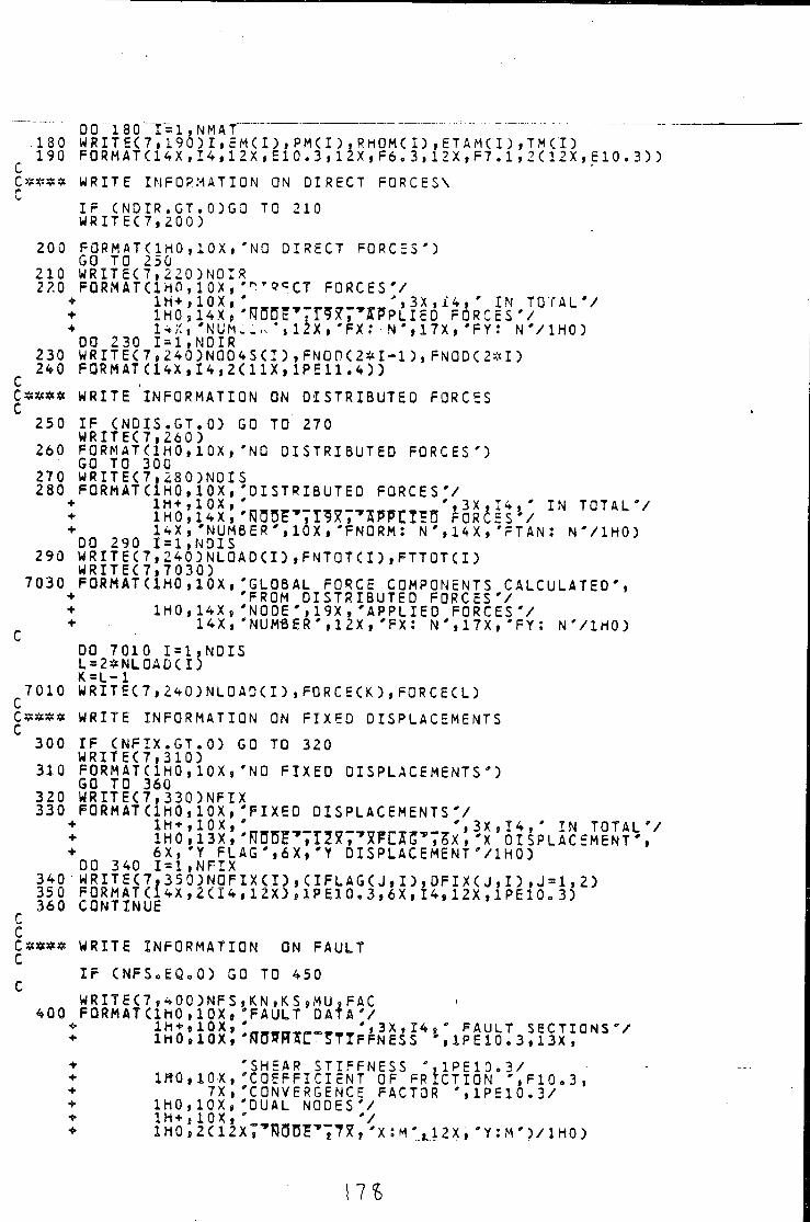
00 1 80 1 = 1 , NM AT 180 WRITE(7,190)I,EM(I),PM<I),RhOM(I),ETAM(I),TM<:i) 190 FORMAT(14X,I4,12X,E10.3,12X,F6.3,12X,F7.1,2(12X,E10.3))
C##** WRITE INFORMATION ON DIRECT FORCESN C I F (NDIR.GT.O)GO TO 210 WRITE(7,200) 200 FORMATC1H0,lOXi 'NO DIRECT FORCES') GO TO 250 210 WRITE(7,220)N0IR 220 FQRMAT(1H0,10X, ' n T s c C T FORCES'/
• 1H+,10X,' ' , 3 X , i 4 , ' IN TOTAL'/ + 1H0,14X, RCSF tT^X^j APPLIED FORCES'/ + 14 X j 'NUMw-.N*»12Xf'FX; N ' , 1 7 X » 'FY! N'/IHO) DO 230 I=1,NDIR 230 WRITE(7,240)N004S(I) ,FNODC 2*1-1 ),FNQDC 2 # I ) 240 FQRMAT(14X,I4,2C11X, 1PE11.4))
C***« WRITE INFORMATION ON DISTRIBUTED FORCES C 250 IF (NDIS.GT.O) GO TO 270 WRITEC7.260) 260 FORMATQHO, 10X , 'NO DISTRIBUTED FORCES') GO TO 300 270 WRITE<7,280)N0IS 280 FORMATC1H0,10X, 'DISTRIBUTED FORCES'/ + l H + ' 1 0 X ' ' ™ , - r , „ - , , „ I . , „ ' » 3 X 1 I 4 , ' IN TOTAL'/ + 1H0,14X , 'ROBE* ,T9T,'ATPCTSD FORCES'/ + 14X, 'NUMBER',10X, 'FNORM! N ' , 14X , ' FT ANi N'/IHO) DO 290 I=1,NDIS 290 WRITEC7,240)NLQADCI) ,FNTOTCI) ,FTTQTCI) WRITEC7.7030)
7030 FQRMATC1H0,10X,'GLOBAL FORCE COMPONENTS CALCULATED', • 'FROM DISTRIBUTED FORCES'/ + 1H0,14X, 'NODE',19X, 'APPLIED FORCES'/ + 14X, 'NUMBER',12X, 'FX! N',17X,'FY: N'/IHO) DO 7010 I=1,NDIS L=2*NL0A0(I) K=L-1
^7010 WRITEC7,2^0)NLOADCI),FORCECK),FORCECL) Csss* WRITE INFORMATION ON FIXED DISPLACEMENTS
300 IF CNFIX.GT.O) GO TO 320 WRITEC7.310) 310 FORMATC1H0,10X, 'NO FIXED DISPLACEMENTS') GO TO 360 320 WRITEC7,330)NFIX 330 FORMATClHOjlOX, 'FIXED DISPLACEMENTS'/ + 1H+,10X,' ',3X,X4,' IN TOTAL'/ + 1H0,13X, 'FJff5E^,m,^FTS5'75x , 'X DISPLACEMENT', + 6X,'Y FLAG',6X,'Y DISPLACEMENT '/1H0) DO 340 I=1,NFIX
340 WRITEC7,35 0)NOFIXCI),(IFLAGCJ,I),DFIXCJ,I),J=1,2) 35 0 F0RMATC14X,2CI4,12X),1PE10.3.6X,14,12X,1PE10,3) 360 CONTINUE C C
C**#$ WRITE INFORMATION ON FAULT IF CNFSoEQoO) GO TO 450
C WRITEC7,<*00)NFS,KN,KS ,MU ,FAC 400 FORMATC1H0,1 OXs 'FAULT DATA'/ • 1H*,10Xi * _ _ _ _ 3 X , 1 4 , ' FAULT SECTIONS "/ • 1H0,10X, 'RffffRAT STIFFNESS ', 1PE10.3,13X ,
+ 'SHEAR STIFFNESS '.1PE10.3/ + IROjIOX, 'COEFFICIENT OF FRICTION '.F10.3, + 7X , 'CONVERGENCE FACTOR '.1PE10.3/ • 1H0 , 10X, 'DUAL NODES'/ • 1H+, 10X , ' V • 1H0 ,2C12X7"'fla*D"E"B77x', 'X SM'j.l2X, 'Y!M')/1H0)
1 7 $
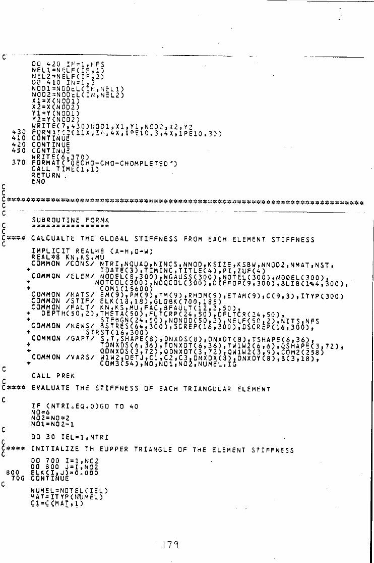
DO 420 Ir=l,MFS NEL1=NELFCIF,1) NEL2=NELFCIF,2) 00 410 IN=1,3 N0D1=NDDELCIN|NEL1) N0D2=N0DtLCIN,NcL2) XlaXCNOOl) X2=XCN0D2) Yl=YCN00l) Y2=YCN0D2) WRITEC7,430)NOD1,X1,Y1,NOD2,X2,Y2
1U ?S5^Tll'1g^lx»--^**X,l«>E10.3,*X,lPE10.3}) 410 CONTINUE
420 CONTINUE 45 0 CONTINUE
WRITEC6.370) 370 FORMAT(OECHO-CHO-CHOMPLETED') CALL TIMEC1.1) RETURN . END C
C
C*********V*****************************^
SUBROUTINE FORM* c C**S* CALCUALTE THE GLOBAL STIFFNESS FROM EACH ELEMENT STIFFNESS
IMPLICIT REALS8 CA-H»0-W) REAL*8 KN,KS,MU COMMON /CONS/ NTRI,NQUAO,NINCS,NNOD,KSI2E , XSBW,NNOD2,NMAT,NST,
• IDATEC3),TIMINC,TITLEC4),PI,ZUFC4) COMMON /ELEM/ NODEL< 8 ,300),NGAUSSC300) , NOTELC300),NOQELC300),
+ NOTCOU300).NOQCOLC3 00).OIFFOPC9,300),8LI8(1^4,300),' COMMON /MATS/ EMC9),PMC9),TMC9),RH3MC9),ETAMC9),CC9,3)tITYPC300) COMMON /STIF/ ELKC13 ,13),GL08KC700, 185) COMMON /FALT/ KN , KS,MU,FAC,3FAULTC12 , 2 , 5 0 ) ,
• DEPTH<50,2).THETAC50).FLTCRPC24, 5 0 ) , 0FLTCR(24 , 5 0 ) , • „ STFBGNC24.50).N0N00C50,2),NELFC50,2),NITS,NFS COMMON /NEWS/ BSTRES C 64 . 300 5 , SCREP06 , 300 ) , DSCR E>(16 , 3 o 5 ) , + STRSTC16,300) COMMON /GAPT/ S,T , SHAPEC8),DNXDSC8),DNXDTC8),TSHAP = C6,36),
+ TDNXDSC6,36),TDNXDTC6,36),TWlW2C6t6),ySHAP5C3,72), + , QDNXDSC3,72),QDNX0TC3,72),QW1W2C3,9),C0M2C258) COMMON /VARS/ Wl W2 , D ET J , CI , C2 ( C3 , DNXDX C 3 ) , DNX 0Y C 8 ) , 8 C 3 , 18 ) , + C0M3C54),N0,N01,N02,NUMEL,IG CALL PREK.
C C**** EVALUATE THE STIFFNESS OF EACH TRIANGULAR ELEMENT C
IF CNTRIeEQ,0)GO TO 40 N0=6 N02=N0*2 N01=N02-1 C DO 30 IEL=1,NTRI C**** INITIALIZE TH EUPPER TRIANGLE OF THE ELEMENT STIFFNESS
DO 700 1=1,N02 00 800 J=I,N02 800 ELKCI.J)=0o000 700 CONTINUE C NUMEL=NOTELCIEL) MAT=ITYPCN\IMEL) C1=C<MAT,1)
1 7 ^
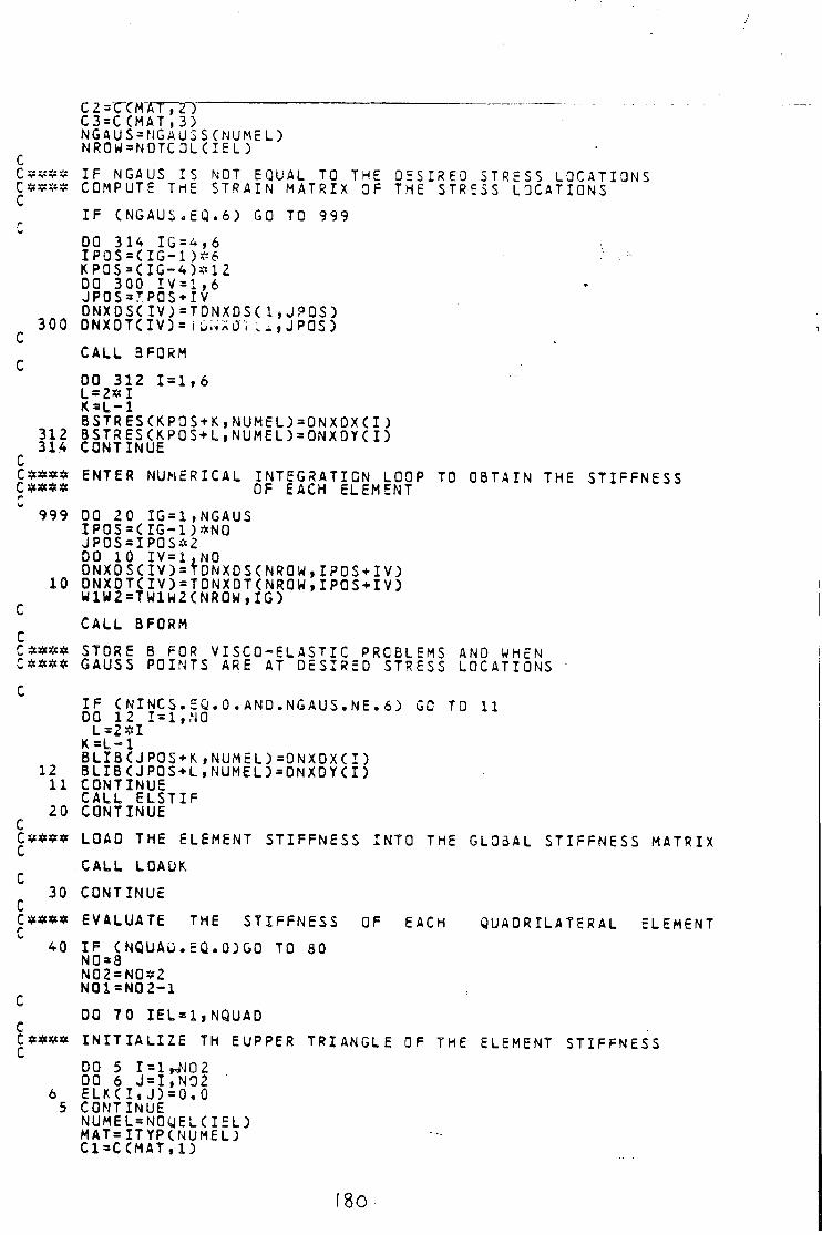
C2=CCMATT2) C3=CCMAT,3) NGAUS=MGAUSSCNUMEL) NROH=NOTCDLCIEL) C C?¥#« IF NGAUS IS NOT EQUAL TO THE DESIRED STRESS LOCATIONS C***s COMPUTE THE STRAIN MATRIX OF THE STRESS LOCATIONS C
IF (NGAUS.EQ.6) GO TO 999 r
00 314 IG=4,6 IP0S=(IG-1)*6 KP0S=(IG-4)*12 DO 300 IV=1,6 JP0S=7PQS+IV ONXOSCIV)=TDNXDS(1,JPQS)
300 DNXDT<IV)= i i ' l iAJi JPOS) C
CALL 3FORM C
DO 312 1=1,6 L = 2 * I K = L-1 BSTRES(KPOS + K,NUMEL.)=DNXDX(I ) 312 BSTRES(K.POS+L,NUMEL) = ONXDYC I ) 31.4 CONTINUE C ENTER NUMERICAL INTEGRATION LOOP TO OBTAIN THE STIFFNESS C**** OF EACH ELEMENT
999 00 20 IG = 1, NGAUS IPOS=(IG-1)*N0 JP0S=IP0S*2 00 10 IV=i,NO DNXOSCIV)=TDNXDS(NROW,IPOS+IV)
10 DNXOTCIV)=TONXDTCNROW,IPOS+IV) W1W2=TW1W2CNR0W,IG) CALL B FORM
C C**#* STORE B FOR VISC0-ELASTIC PROBLEMS AND WHEN C*##* GAUSS POINTS ARE AT DESIRED STRESS LOCATIONS ' C
IF (NINCS.EQ.O.AND.NGAUS.NE.6) GO TO 11 00 12 1=1,NO L=2*I K=L-1 BLIBCJ POS + K. ,NUMEL)=ONXDXCI ) 12 BLIB<JPOS+L,NUMEL)=DNXDY<I) 11 CONTINUE CALL ELSTIF
20 CONTINUE C C**** LOAD THE ELEMENT STIFFNESS INTO THE GL05AL STIFFNESS MATRIX
CALL LOAUK C
30 CONTINUE C C***« EVALUATE THE STIFFNESS OF EACH QUADRILATERAL ELEMENT
40 I F (NQUAD.EQ.O)GO TO 80 N0 = 8 N02=NO*2 N01=N02-1
C DO 70 IEL=1,NQUAD
C*#** INITIALIZE TH EUPPER TRIANGLE OF THE ELEMENT STIFFNESS DO 5 I=1*N02 DO 6 J=I,N02 6 ELK(I,J)=0.0 5 CONTINUE NUMEL=NOyEL(IEL) MAT=ITYPCNUMEL; C1=CCMAT,1)
! 8 0
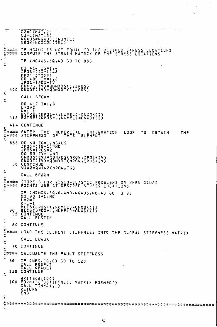
C2=C(MAT,2 ) C3=CCMAT,3) NGAUS=NGAUSS(NUMEL) NRO^=NOQCQLCIEL)
C * * S * I F NGAUS I S NOT EQUAL TO THE OESIREO STRESS LOCATIONS C * * * 3 COMPUTE THE STRAIN MATRIX OF THE STRESS LOCATIONS
I F ( N G A U S . E Q . 4 ) GO TO 888 C
DO 414 I G = 1 , 4 I P O S * ( I G - l ) * 8 K P C ! DO 400 I V = 1 , 3 JPOS=IPOS+IV DH>ww;IV)»QDNXDSCl »JPOS)
400 DNXDTCIV)=Q0NXDT(1 ,JPOS)
CALL 8 FORM C
DO 41^ 1 = 1 , 8 L = 2 * I K=L-1 BSTRESCKPOS+K,NUMEL)=ON X D X ( I )
412 BSTRESCKPOS+LiNUMEL)=DNXDYCI)
414 CONTINUE C C*=* * * ENTER THE NUMERICAL INTEGRATION LOOP TO OBTAIN THE C * $ * * S T I F F N E S S OF THIS ELEMENT C
888 00 60 IG=1,NGAUS I P O S = C I G - 1 ) * N 0 J P 0 S = I P 0 S * 2 00 50 IV=1,N0 ONXOSCIV) = QDNXDS<NROW,IPOS-HV) ONXOTCIV)=QDNXDT<NROW,IPOS+IV)
50 CONTINUE W1W2=QW1W2CNR0U,IG)
C CALL B FORM
C C 3 * * 5 STORE B FOR V I S C O - E L A S T I C PROBLEMS OR WHEN GAUSS C s * # # POINTS ARE AT DESIRED STRESS LOCATIONS
I F C N I N C S . E Q . O . A N D . N G A U S . N E . 4 ) GO TO 95 00 90 1=1,NO L = 2 * I K=L-1 BLIBCJPOS+K,NUMEL)=ONXDXCI)
90 B L I B ( J P Q S + L , N U M E L ) = D N X D Y C I ) 95 CONTINUE
CALL E L S T I F C
60 CONTINUE C C * * * * .LOAD THE ELEMENT S T I F F N E S S INTO THE GLOBAL S T I F F N E S S MATRIX
CALL LOADK C
70 CONTINUE C C * * # * CALCUALTE THE FAULT S T I F F N E S S
80 I F ( N F S . E Q . O ) GO TO 120 CALL PREFLT CALL K.FAULT
120 CONTINUE W R I T E C 6 , 1 0 0 )
100 FORMATC ' O S T I F F N E S S MATRIX FORMEO') CALL T I M c ^ l . U RETURN ENO
C C
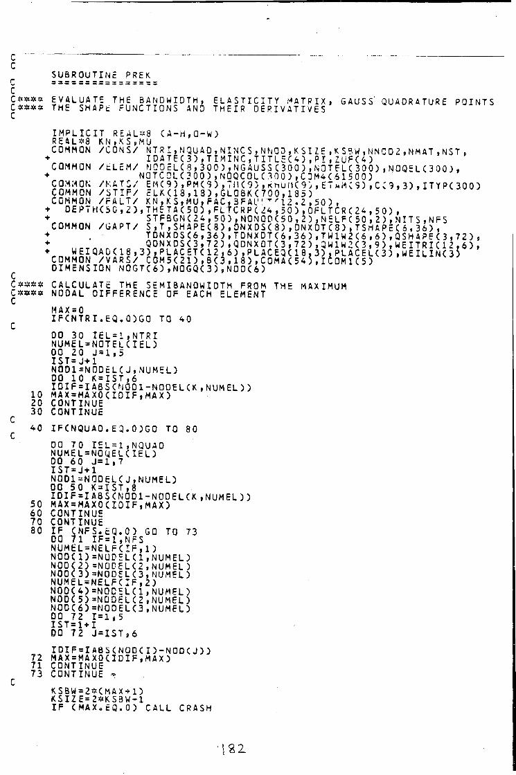
SUBROUTINE PREK
£ * * * « EVALUATE THE 3ANDWIDTH, E L A S T I C I T Y MATRIX, GAUSS QUADRATURE POINTS C * * * * THE SHAPE FUNCTIONS AND THEIR D E R I V A T I V E S
I M P L I C I T REAL~8 C A - H , 0 - W ) R E A L * 8 KN,KS,MU COMMON / C O N S / N T R I , NQUAO , NINCS ,NNOD , K S I ZE ,K,S?W,NNOD2,NMAT,NST.
I D A T E C 3 ) , T I M I N G , T I T L E C O , P I i Z U F C O COMMON / c L E M / NOD ELC 8 , 300 ) , NGAUSS( 300 ) ,NOTELC 3 0 0 ) , N O Q E L C 3 0 0 ) ,
• NOTCOLC300) ,NOQCOLC300) .C0M4C61500) COMMON / M A T S / EMC 9 ) , PMC 9 ) , TfK 9 ) , khuMC 9*, , E T M H < S ) , C C 9 , 3 ) , I T Y P C 3 COMMON / S T I F / ELKC18 , 1 3 ) , G L O B K C 700 , 185 ) COMMON / F A L T / K N , K S , M U , F AC , 3 F A I". ' I 2 . 2 , 50 ) ,
+ D E P T H C 5 C , 2 ) , T H E T A C 5 0 ) , F L T C R P C 2 4 , 5 0 ) , D F L T C R C 2 4 , 5 0 ) , + S T F B G N C 2 4 , 5 0 ) , N O N O O C 5 0 , 2 ) , N E L F C 5 0 , 2 ) , N I T S , N F S
S , T , S H A P E C 8 ) , D N X D S C 8 ) , 0 N X D T C 8 ) , T S H A P E C 6 , 3 6 ) , T D N X D S C 6 , 3 6 ) , T D N X D T C 6 , 3 6 ) , T W 1 W 2 C 6 , 6 ) , Q S H A P E C 3 , 7 2 ) o n w y n < ; M . 7 ? , i . n n w v n T n . 7 i > _ T u i L i c i a\ u c T - r n T ^ i - > ^ N
S T F B G N C 2 4 , 5 0 ) , N 0 N 0 D C 5 0 , 2 ) , N E L F C 5 0 , 2 ) , N I T S COMMON / G A P T / " ~ -
+ '<-"•> nuo w i J O ; I I U H A U H O I J O ; I i m « a o i o ; ) i j j n A ) ' c U i + , Q D N X D S C 3 , 7 2 ) , Q D N X D T C 3 , 7 2 ) , a w i W 2 C 3 , 9 ) , W E I T R I C 1 2 , 6 ) • WEIQADCI 8 , 3 ) , P L AC ETC 1 2 , 6 ) , P L A C E Q C 1 8 , 3 ) , P L A C E L C 3 ) . W E I L I N C 3 )
CDMMON / V A R S / COM5C21) , 3 C 3 , 1 8 ) , COMAC54) , ICOM1C5) DIMENSION N0GTC6) ,NQGQC3) ,N0DC6)
C * * * # CALCULATE THE SEMIBANOWIDTH FROM THE MAXIMUM C =C*xs«! NODAL D I F F E R E N C E OF EACH ELEMENT C
MAX = 0 I F C N T R I . E Q . 0 ) G 0 TO 40 DO 30 I E L = 1 , N T R I NUMEL=NOTELCIEL) 00 20 J = l , 5 I S T = J + l N0D1=N0DELCJ.NUMEL) DO 10 K = I S T , 6 I D I F = IABSCNOD 1-NODELCK,NUMEL) )
10 MAX=MAXOCIDIF,MAX) 20 CONTINUE 30 CONTINUE
40 IFCNQUAD.EQ.0 )GO TO 80
00 70 IEL=1,NQUAD NUMEL=NOQELCIEL) 00 60 J = l , 7 IST=J+1 N0D1=NQDELCJ,NUMEL) 00 50 K = I S T , 8 I D I F = I A 8 S C N 0 D 1 - N 0 D E L C K , N U M E L ) )
50 MAX=MAXOCXDIF,MAX) 60 CONTINUE 70 CONTINUE 80 I F C N F S . E Q . O ) GO TO 73
DO 71 I F = 1 , N F S N U M E L = N E L F C I F , 1 ) N00C1)=NUDELC1,NUMEL) N00C2)=NODELC2 » NUMEL ) NOOC 3)=N0DELC3,NUMEL) NUMEL=N£LFCIF ,2 ) N0DC4)=NODELCl ,NUMEL) NOD(5)=NODELC2,NUMEL) N0DC6)=N00ELC3,NUMEL) DO 72 1=1,5 I S T = 1 + I DO 72 J = I S T , 6
I D I F = I A B S C N O D C l ) - N O D C J ) ) 72 MAX=MAXOCIDIF,MAX) 71 CONTINUE 73 CONTINUE *
KSBW=2*CMAX+1) K S I Z E= 2SK.S3W-1 I F CMAX. tQ .O) CALL CRASH
1 8 2
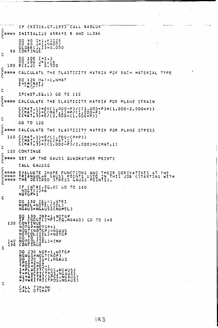
I F ( K S I 2 t . G T . 1 8 5T~CA L L 3A 0 1 U K " C C * * x t * I N I T I A L I Z E A R R A Y S B AND G L O B K C
DO 9 0 1 = 1 , K S I Z E D O 9 0 J = l , N N 0 D 2 G L D B K C J , I ) = O . O D 0
9 0 C O N T I N U E C
DQ 100 1 = 1 , 3 DO 100 J = l , 1 6
100 B C I . J ) = 0 . 0 0 0 C C S S S * C A L C U L A T E T H E E L A S T I C I T Y M A T R I X FOR E A C H M A T E R I A L T Y P E C
DO 1 2 0 MA r = 1 , N M A T E = E M ( M A T )
: ~ '« i' • C
I F ( N S T . E Q . l ) GO TO 1 1 0 C C » « * * C A L C U L A T E T H E E L A S T I C I T Y M A T R I X FOR P L A N E S T R A I N C
C ( M A T , l ) = E * ( 1 . 0 D O - P ) / ( ( 1 . 0 O 0 + P ) * ( 1 . 0 D 0 - 2 . 0 D 0 * P ) ) C C M A T , 2 ) = C ( M A T . 1 ) * P / ( 1 . 0 D O - P ) C C M A T , 3 ) = E / ( 2 . 6 0 0 * ( 1 . 0 D O + P ) )
GO T O 1 2 0 C C * * * $ C A L C U L A T E T H E E L A S T I C I T Y M A T R I X F O R P L A N E S T R E S S
1 1 0 C C M A T , l ) = E / ( 1 . 0 D O - ( P * P ) ) C ( M A T , 2 ) = P * C ( M A T , 1 )
C C M A T , 3 ) = ( ( 1 , 0 0 0 - P ) / 2 . 0 0 0 ) * . C ( M A T , 1 )
1 2 0 C O N T I N U E C C * * * * S E T UP T H E G A U S S Q U A D R A T U R E P O I N T S C
C A L L G A U S S Q C C * * * * E V A L U A T E S H A P E F U N C T I O N S AND T H E I R D E R I V A T I V E S AT T H E C * * * * T R I A N G U L A R G A U S S P O I N T S U S E D I N T H I S J O B ( S T A R T I N G W I T H C * # * « T H E D E S I R E D S T R E S S G A U S S P O I N T S ) . C
I F ( N T R I . E Q . O ) GO TO 1 6 0 N 0 G T ( 1 ) = 6
N 0 T G P * = 1 C
DO 1 5 0 I E L = 1 , N T P I N U M E L = N Q T E L ( I E L ) N G A U S = N G A U S S ( N U M 5 L )
DO 1 3 0 I M P = 1 . N 0 T G P I F ( N O G T ( I M P ) . E Q . N G A U S ) GO TO 1 4 0
1 3 0 C O N T I N U E N O T G P = N O T G P + 1 N O G T ( N O T G P ) = N G A U S N O T C O L ( I E L ) = N Q T G P GO T O 1 5 0
1 4 0 N O T C 0 L ( I E L ) = I M P 1 5 0 C O N T I N U E
C 0 0 2 3 0 N 0 P = 1 , N 0 T G P N G A U S = N O G T ( N O P ) DO 2 2 0 I G = 1 , N G A U S S P 0 S = 2 * I G T P 0 S = S P 0 S - 1 S = P L A C E T ( S P O S , N G A U S ) T - P L A C E T C T P O S . N G A U S ) W 1 = W E I T R I C S P C $ , N G A U S ) W 2 = W E I T R I ( T P 0 S , N G A U S )
C C A L L TSHAF^N C A L L D T S H A P
123
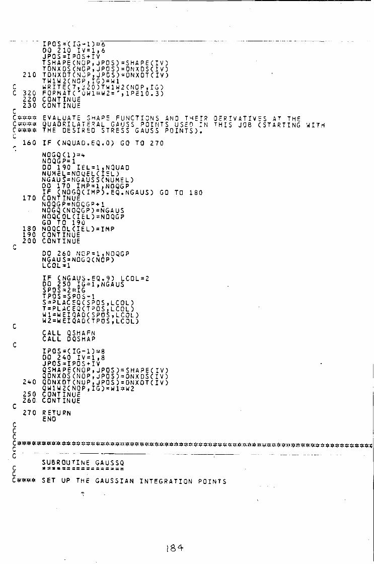
I P O S = < I G - 1 ) * 6 " " 0 0 2 1 0 I V = 1 , 6 J P O S = I P O S + I V T S H A P E C N G P , J P O S ) = S H A P E C I V ) T 0 N X D S ( N O P , J P O S ) = 0 N X D S ( I V )
2 1 0 T D N X D T C N U P , J P C S ) = ONX DT C I V ) T W 1 W 2 ( N 0 P , I G ) = W 1
C W R I T E C 7 , 3 2 0 ) T W 1 W 2 < N O P , I G ) C 3 2 0 F O R M A T C ' 0 W l * W 2 » ' i l P E 1 0 . 3 )
2 2 0 C O N T I N U E 2 3 0 C O N T I N U E
C C $ * * S E V A L U A T E S H A P E F U N C T I O N S AMD T H E I R D E R I V A T I V E S AT T H E C * * # * Q U A O R I L A T E R A L G A U S S P O I N T S U S E D I N T H I S J O B ( S T A R T I N G W I T H
T H E D E S I R E D S T R E S S G A U S S P O I N T S ) . C
1 6 0 I F C N Q U A D . E Q . O ) GO TO 2 7 0
N O G Q Q ) = <» N O Q G P = 1 DO 1 9 0 I E L = 1 , N Q U A 0 N U M c L = N O U E L C I E L ) N G A U S " = N G A U S S ( N U M E L ) DO 1 7 0 I M P = 1 , N 0 Q G P I F ( N O G Q C I M P ) . E Q . N G A U S ) GO TO 1 8 0
1 7 0 C O N T I N U E N 0 Q G P = N 0 C G P + 1 N O G Q C N O G G P ) = N G A U S N 0 Q C 0 L C I E L ) = N 0 Q G P GO T O 1 9 0
1 8 0 N O Q C O L C I E L ) = I M P 1 9 0 C O N T I N U E 2 0 0 C O N T I N U E
r DO 2 6 0 N C P = 1 , N 0 Q G P N G A U S = N O G Q ( N O P ) L C 0 L = 1
I F ( N G A U S . 5 Q . 9 ) L C 0 L = 2 DO 2 5 0 I G = 1 , N G A U S S P 0 S = 2 * I G T P 0 S = S P 0 S - 1 S = P L A C E Q C S ? O S , L C O L ) T«PLACEQCTi'QSiLCOL) W 1 = W E I Q A D ( S P O S , L C O L ) W 2 = W E I Q A D ( T P 0 S , L C O L )
CALL Q S H A F N CALL D Q S H A P
C I P 0 S = ( I G - 1 ) * 8 DO 2 4 0 I V = 1 , 8 J P O S = I P O S + I V Q S H A P E C N Q P , J P O S ) = S H A P E C I V ) Q O N X D S ( N O P , J P 0 S 5 = D N X 0 S C I V )
2 4 0 Q D N X D T C N U P , J P O S ) = D N X D T C I V ) QW1W2C N O P , I G ) = W 1 * W 2
2 5 0 C O N T I N U E 2 6 0 . C O N T I N U E
C 2 7 0 R E T U R N
E N D C c c
C S U B R O U T I N E G A U S S Q
C * * * * S E T U P T H E G A U S S I A N I N T E G R A T I O N P O I N T S
184
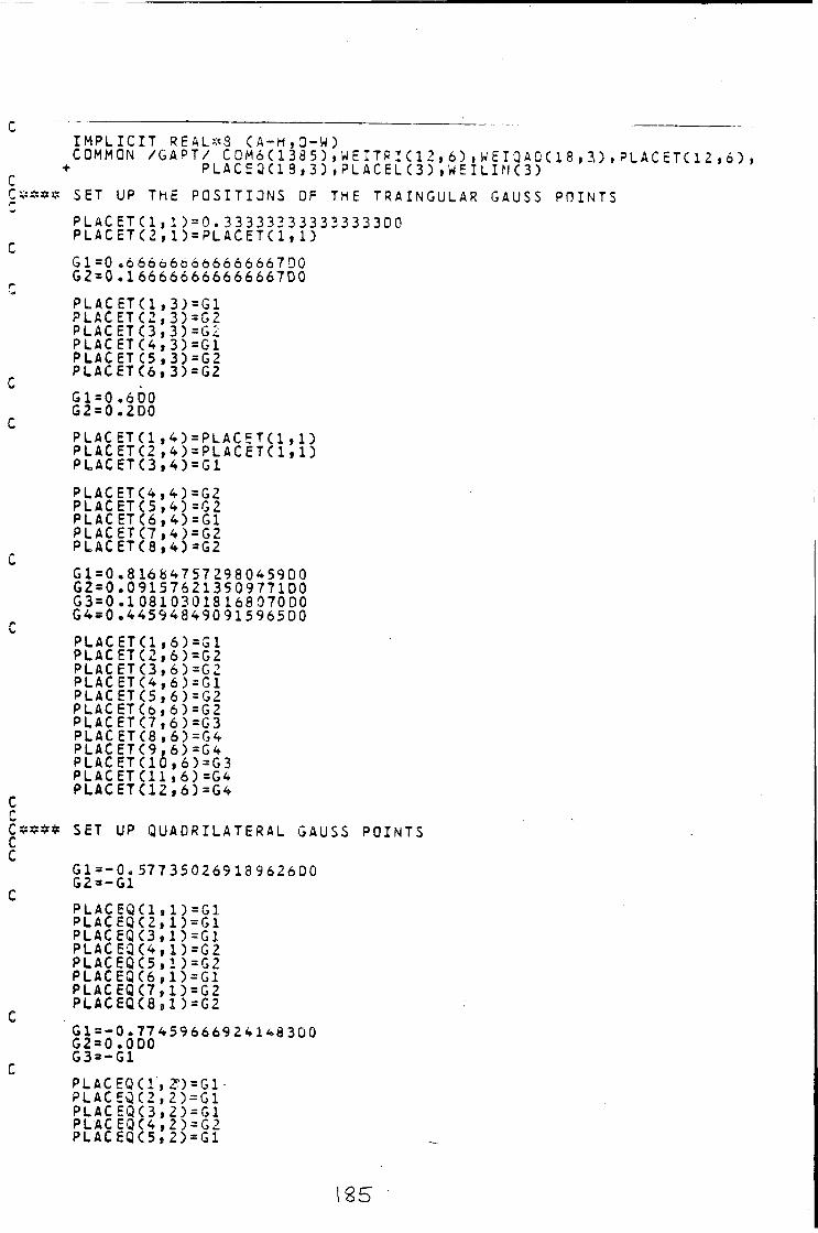
I M P L I C I T R E A L M S CA-M,3-W) COMMON / G A P T / C0M6( 1 38 5 ) , W E I T P I C 1 2 , 6 5 , W E I Q A 0 C 1 8 , 3 . ) , P L A C E T ( 1 2 ,
• P L A C E Q C 1 3 , 3 ) , P L A C E L ( 3 ) , W E I L I N < 3 )
SET UP THE POSITIONS OF THE TRAINGULAR GAUSS POINTS
P L A C E T C 1 i 1 ) = 0 . 3 3 3 3 3 3 3 3 3 3 3 3 3 3 3 D 0 P L A C E T C 2 , 1 ) = P L A C E T ( 1 , 1 )
G l = 0 . 6 66 66o66666666700 G 2 = 0 . 1 6 6 6 6 6 6 6 6 6 6 6 6 6 7 0 0
P L A C E T ( 1 , 3 ) = G 1 P L A C E T C 2 , 3 ) = G 2 P L A C E T C 3 , 3 ) = G 2 P L A C E T ( 4 , 3 ) = G 1 P L A C E T C 5 , 3 ) = G 2 P L A C E T C 6 , 3 ) = G2
G1 = 0 .6D0 G2=0.2D0
P L A C E T C l , 4 ) = PLACET(1 , 1 ) P L A C E T C 2 , 4 ) = P L A C E T C 1 , 1 ) P L A C E T C 3 , 4 ) = G 1
P L A C E T ( 4 f 4 ) = G 2 P L A C E T ( 5 , 4 ) = G 2 P L A C E T ( 6 , 4 ) = G 1 P L A C E T C 7 , 4 ) = G 2 P L A C E T C 8 , 4 ) = G 2
G l = 0 . 8 1 6 8 4 7 5 7 2 9 8 0 4 5 9 0 0 G2 = 0 . 091576213509771D0 G 3 = 0 . 1 0 8 1 0 3 0 1 8 1 6 8 0 7000 G4=0 .445948490 915 965 00
P L A C E T C 1 , 6 ) = G 1 P L A C E T C 2 , 6 ) = G 2 P L A C E T ( 3 , 6 ) = G 2 P L A C E T C 4 , 6 ) = G 1 P L A C E T ( 5 , 6 ) = G 2 P L A C E T C 6 , 6 ) = G 2 P L A C E T C 7 , 6 ) = G 3 P L A C E T C 8 , 6 ) = G 4 P L A C E T C 9 . 6 ) = G 4 P L A C E T C 1 0 , 6 ) = G 3 P L A C E T ( 1 1 , 6 ) = G 4 P L A C E T C 1 2 , 6 ) = G 4
6 )
SET UP QUADRILATERAL GAUSS POINTS
G l = - 0 . 5 7 7 3 5 0 2 6913962600 G2=-G1
P L A C E Q C l f 1 ) = G 1 PLACEQC2,1 )=G1 P L A C E Q ( 3 , 1 ) = G 1 P L A C E Q ( 4 , 1 ) = G 2 P L A C E Q C 5 , 1 ) = G 2 PLACEQC6,1 )=G1 P L A C E Q C 7 , 1 ) = G 2 P L A C E Q C 8 S 1 ) = G 2
G l = - 0 . 7 7 4 5 9 6 6 6 9 2 4 1 4 8 3 0 0 G2=0.ODO G3=-G1 PLACEQC1,2 )=G1 PLACEQC2,2 )=G1 PLACEQC3,2 )=G1 P L A C E Q C 4 , 2 ) = G 2 PLACEQC5,2 )=G1
125
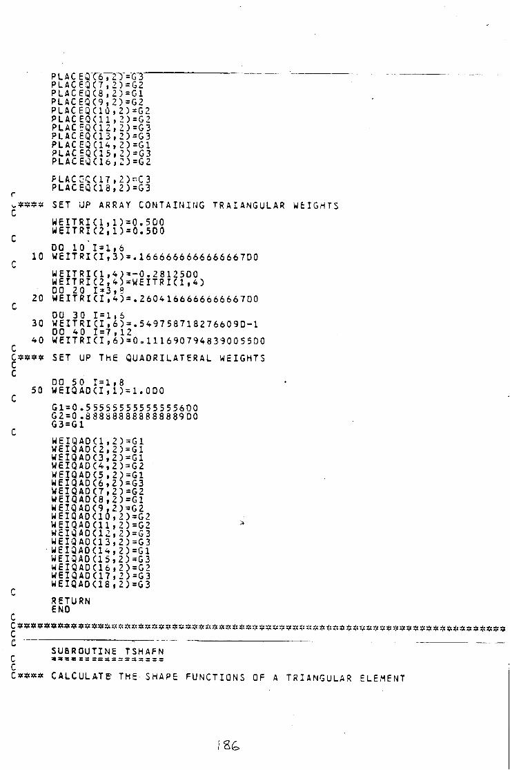
PL AC E"QT6T2T=G"3 P L A C E Q ( 7 , 2 ) = G 2 PLACEQC8,2 )=G1 PLACEQC9 ,2 )=G2 PLAC EQC10 , 2)=G2 PLAC EQC11 ,2 )=G2 P L A C E Q C 1 2 , 2 ) = G 3 P L A C E Q C 1 3 , 2 ) = G 3 PLACEQC14 ,2 )=G1 P L A C E Q ( 1 5 , 2 ) = G 3 P L A C E Q C 1 6 , 2 ) = G 2
P L A C £ C ( 1 7 , 2 ) ^ C 3 P L A C E Q ( 1 3 , 2 ) = G 3
^ZitZZ SET UP ARRAY CONTAINING TR AI ANGULAR WEIGHTS
W E I T R I C 1 , l ) = 0 . 5 O 0 W E I T R I ( 2 , 1 ) = 0 . 5 D 0
C DO 10 1=1,6
10 W E I T R I C I i 3 ) * . 1 6 6 6 6 6 6 6 6 6 6 6 6 6 6 7 D 0 W E I T R K 1 , 4 ) = - 0 . 2812500 W E I T R I C 2 , 4 ) = W E I T R I ( 1 , 4 ) DO 2 0 1=3,9
20 W E I T R I C I ,<O=.2604166666666667D0
DO 30 1=1,6 30 WEITRI ( I » 6 ) = . 5 4 9 7 5 8 7 1 8 2 7 6 6 0 9 0-1
DO 40 1=7 ,12 40 W E I T R I C I , 6 ) = 0 . 1 1 1 6 9 0 7 9 4 8 3 9 0 0 5 5 0 0
C * * 3 * SET UP THE QUADRILATERAL WEIGHTS C
DO 50 1=1,8 50 W E I Q A D C I , 1 ) = 1 . 0 0 0
G1 = 0 . 5 5555555555555600 G2 = 0 . 8 8 8 8 8 8 8 8 8 8 8 8 8 8 9 DO G3 = G1
C WEIQADCI ,2 )=G1 WEIQADC2,2)=G1 WEIQADC3,2)=G1 W6IQADC4,2)=G2 WEIQADC5,2)=G1 WEIQADC6,2)=G3 WEIQAD(7 ,2 )=G2 WEIQAOC8,2)=G1 WEIQADC9,2)=G2 WEIQAOC10,2)=G2 WEIQADC11, 2)=G2 : s
W E I Q A O a Z , 2) = G3 WEIQA0C13,2 )=G3 WEIQA0C14,2)=G1 WEIQADC15,2)=G3 WEIQADC16,2)=G2 WEIQADC17,2)=G3 WEIQADC18,2)=G3 RETURN END
C
C ' SUBROUTINE TSHAFN
c C * * * « CALCULATE THE SHAPE FUNCTIONS OF A TRIANGULAR ELEMENT
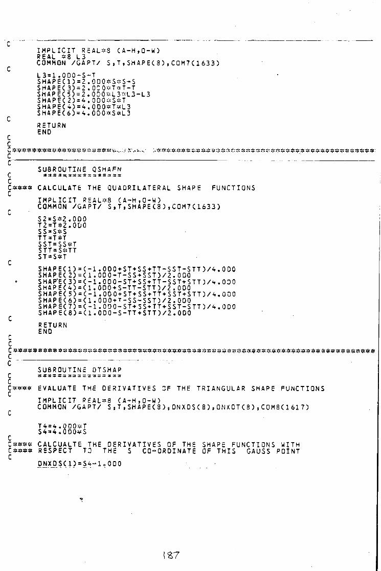
c I M P L I C I T R£AL*8 CA-H.O-W) REAL * 8 L3 COMMON / G A P T / S , T , SH AP E ( 8 ) , C OM7 C 1 63 3 ) L 3 = 1 . 0 D 0 - S - T S H A P E C 1 ) = 2 . 0 D 0 * S * S - S S H A P E C 3 ) s 2 . 0 0 0 # T * T - T S H A P E ( 5 ) = 2 . 0 D 0 * L 3 * L 3 - L 3 S H A P E < 2 ) a 4 . 0 0 0 * S * T S H A P E C 4 ) = 4 . 0 D O * T * L 3 S H A P E C 6 ) * 4 . 0 0 0 * S * L 3
C RETURN END
C C L. <v» ^ ^ * ^**r* -v * v > ^ J? * i * * ~ v* ,— . 1 ,«- ,•• ,•-.»••,•» -v -s» -v> i" - v * ' ^ -i» - . 5 " . * -f» -».» 7fi v -i* ?»* -s* ^ 5 3?;«*£ *»« *r
C c
SUBROUTINE QSHAFN C = = = = =.== = = = = = = = = = c C * # * 3 CALCULATE THE QUAORILATERAL SHAPE FUNCTIONS C
I M P L I C I T REALS8 ( A - H . O - W ) COMMON / G A P T / S , T , S H A P E C 8 ) , C O M 7 ( 1 6 3 3 ) S 2 = S * 2 . 0 D 0 T 2 = T * 2 . 0 D 0 S S = S * S TT=T*T S S T = S S * T STT=S*TT ST=S*T
C S H A P E C 1 ) = C - 1 . 0 D 0 + S T + S S + T T - S S T - S T T ) / 4 . 0 D 0 SHAPEC2) = C 1 . 0 0 0 - T - S S + S S T ) / 2 . 0 00 SHAP'E(3) = < - 1 . 0 D 0 - S T + S S + T T - S S T + S T T ) / 4 . 0 D 0 S H A P E C 4 ) = C 1 . 0 0 0 + S - T T - S T T ) / 2 . 0 D O S H A P E C 5 ) = C - 1 . 0 D 0 + S T + S S + T T + S S T + S T T ) / 4 . 0 D 0 S M A P E C 6 ) = C 1 . 0 D O + T - S S - S S T ) / 2 . 0 0 0 S H A P E C 7 ) = C - 1 . 0 D 0 - S T + S S + T T + S S T - S T T ) / 4 . 0 D 0 S H A P E C 8 ) = C 1 . 0 D 0 - S - T T + S T T ) / 2 . 0 D 0
C RETURN END
r v
C C C '
SUBROUTINE DTSHAP C ================= C O * * * EVALUATE THE D E R I V A T I V E S OF THE TRIANGULAR SHAPE FUNCTIONS C
I M P L I C I T REALS8 ( A - H , Q - W ) COMMON / G A P T / S , T , SHAPEC3 ) , D N X 0 S C 8 ) , O N X D T ( 8 ) , C 0 M 8 C 1 6 1 7 )
T 4 = 4 „ 0 D 0 * T S 4 = 4 . 0 0 0 * S
C Zz#*if CALCUALTE THE D E R I V A T I V E S OF THE SHAPE FUNCTIONS WITH C**x t * RESPECT TD THE S CO-ORDINATE OF THIS GAUSS POINT C
DNXDSCl )=S4- loOOO
(27
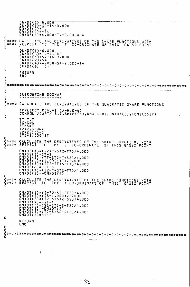
DNXDSC 3) = 0 .'0D"C ~~ " " DNXDSC5) = S4-*-T4-3.0DO DNXDSC 2) = T4 DNXDSC4)=-T<* D N X D S C 6 ) = 4 . O D O - T 4 - 2 . 0 D 0 * S 4
C C * * * ? CALCULATE The D E R I V A T I V E S OF THE SHAPE FUNCTIONS WITH C * * * f c RESPECT TO THE T CO-ORDINATE OF THIS GAUSS POINT
DNXDTC1)=0.0D0 DNXDT(3 )=T4 -1 .0D0 DNXDTC 5) = S4 + T4 -3 .ODO DNXDTC 2) = S4 O N X D T C 4 ) = 4 . O D 0 - S 4 - 2 . 0 D O * T 4 DNXDTC6: : v c RETURN END
C C
c t
SUBROUTINE DQSHAP
c " C * * * « CALCULATE THE D E R I V A T I V E S OF THE QUADRATIC SHAPE FUNCTIONS
I M P L I C I T R E A L * 9 C A - H , 0 - W ) COMMON / G A P T / S i T , SHAPEC8) ,DNXDSC8) ,DNXDTC3) ,C0M8C1617 ) TT=T*T S S = S * S ST=S*T T2=2 .0D0*T S2 = 2 .ODOvS S T 2 = 2 . 0 D 0 * S T
C C * * * « CALCULATE THE D E R I V A T I V E S OF THE SHAPE FUNCTIONS WITH C * $ * * RESPECT TO THE S CO-ORDINATE OF THIS GAUSS POINT
D N X D S C 1 ) = C S 2 + T - S T 2 - T T ) / 4 . 0 D 0 DNXOSC 2) = S T - S DNXDSC3) = C T T - S T 2 - T + S 2 ) / 4 . OOO D N X D S C 4 ) = C 1 . 0 D 0 - T T ) / 2 . 0 D 0 DNXDSC 5) = CST2 + TT + S2 + T ) / 4 . 0 D 0 D N X 0 S C 6 ) = - S T - S DNXDS(7)=CS2-T+ S T 2 - T T ) / 4 . 000 DNXDS<8)=-0NXDSC4)
C * * S * CALCULATE THE D E R I V A T I V E S OF THE SHAPE FUNCTIONS WITH C * * * * RESPECT TO THE T CO-ORDINATE OF THIS GAUSS POINT
D N X D T C 1 ) = C S + T 2 - S S - S T 2 ) / 4 . 0 D 0 D N X D T C 2 ) = C S S - 1 . 0 0 0 ) / 2 . O D O D N X 0 T C 3 ) = C T 2 - S + S T 2 - S S ) / 4 . 0 D 0 0 N X D T C 4 ) = - S T - T ONXDTC5)=CSS+ST2+S+T2 ) / 4 .000 DNXDTC6)=-0NX0TC2) D N X D T C 7 ) = ( T 2 - S + S S - S T 2 ) / 4 . 0 D 0 DNXDTC8)=ST-T
RETURN END
I 8%
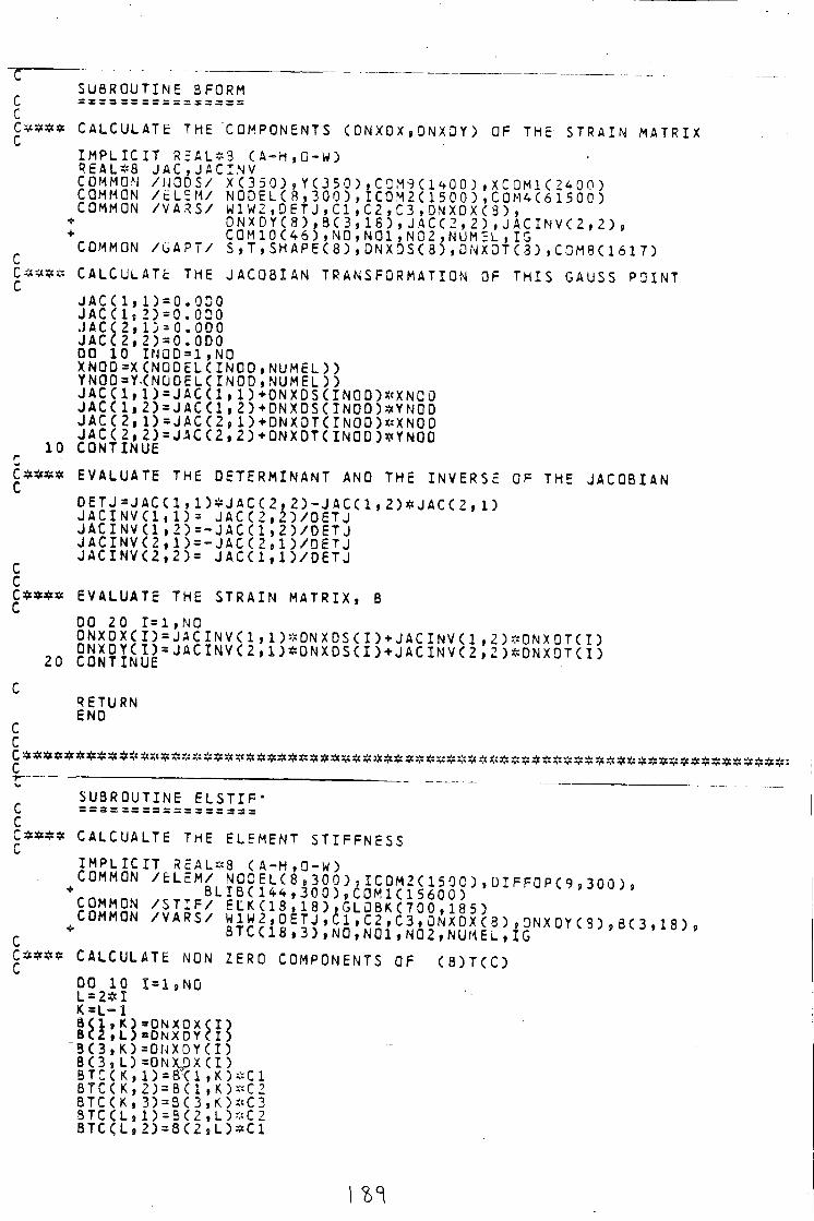
c C * * s * CALCULATE THE COMPONENTS CONXDX,DNX3Y) OF THE STRAIN MATRIX
I M P L I C I T R5ALS3 ( A - H . O - W ) REAL*8 J A C J A C I N V COMMON /NODS/ XC3 5 0 ) , Y C 3 5 0 ) , CQM9(1400) , XCOM1C2400 ) COMMON / E LE M/ NODELC8, 3 0 0 ) , I COM2C 1 5 0 0 ) , C 0 M 4 ( 6 1 5 0 0 ) COMMON / V A R S / W 1 W 2 , D E T J , C 1 , C 2 , C 3 , ON XDX(3 ) ,
• D N X D Y ( 8 ) , B ( 3 , 1 8 ) , J A C C 2 , 2 ) , J A C I N V < 2 t 2 ) , + C0M10C46) ,N0 ,N01 ,N02 ,NUMEL , IG
COMMON /GA P T / S , T , S H A P E C 8 ) , D N X 0 S C 8 ) , D N X O T C 3 ) , COM8C1617) C * « c * CALCULATE THE J ACQBIAN TRANSFORMATION OF THIS GAUSS POINT
J A C C 1 , 1) = 0.0D0 J A C C 1 , 2 ) = 0 . 0 0 0 J A C ( 2 » l ) = 0 . 0 O 0 J A C C 2 , 2 ) = 0 . 0 D 0 DO 10 INQD=1,N0 XNOD=XCNQDELCIN0D,NUMEL)) YNOO=Y.(NODELCINOD,NUMED) J A C C 1 , 1 ) = J A C C 1 , 1 ) + 0 N X D S C I N 0 D ) * X N C D J A C C l f 2 ) = J AC C I ,2 )+DNXDSCIN0D)*YN0D J A C C 2 , 1 ) = J A C C 2 , 1 ) + D N X D T C I N 0 D ) * X N 0 0 JACC 2 , 2 )=JACC2,2)+ONXDTCINO0)*YNO0
10 CONTINUE r C * * * * EVALUATE THE DETERMINANT ANO THE INVERSE OF THE JACOBIAN
0 E T J = J A C C 1 , 1 ) * J A C C 2 , 2 ) - J A C C 1 , 2 ) * J A C C 2 , 1 ) J A C I N V C 1 , 1 ) = J A C ( 2 , 2 ) / D E T J JAC I N V C I , 2 ) = - J AC C I , 2 ) / D E T j J A C I N V C 2 , l ) = - J A C C 2 , l ) / D E T j J A C I N V C 2 , 2 ) = J A C C l , l ) / D E T J
C * * * s EVALUATE THE STRAIN MATRIX, B
DO 20 1=1,NO S N £ S S m = J A C I N V ( l , l ) * D N X D S C I ) + J A C l N V C l , 2 ) * 0 N X 0 T C I )
20 C O N T I N U E * J A ^ ' 2 J*DNX0TCI3 C
RETURN END
C C
r — — SUBROUTINE E L S T I F •
C --======
C * * * * CALCUALTE THE ELEMENT S T I F F N E S S
C
I M P L I C I T REALS8 C A - H , 0 - W ) COMMON / E L E M / N0DELC8 , 3 0 0 ) , I C 0 M 2 C 1 5 Q 0 ) , D I F F 0 P C 9 , 3 0 0 ) »
' „ B L I B C 1 4 4 , 3 0 0 ) , C O M 1 C 1 5 6 0 0 ) ' £2222!^ ^ S T I F / E L K C 1 8 , 1 8 ) , G L 0 B K C 7 0 0 , 185) COMMON / V A R S / W 1 W 2 , D E T J , t 1 , C 2 , C 3 , D N X D X C 8 ) , D N X 0 Y C 3 ) , 8 C 3 , 1 8 ) ,
B T C C 1 8 , 3 ) , N 0 , N 0 1 , N 0 2 , N U M E L , I G ' ' C * * S * CALCULATE NON ZERO COMPONENTS OF C B ) T C C )
00 10 1=1,NO L = 2 * I K=L-1 a C l . K J a Q N X O X C I ) B C 2 , L ) * D N X D Y C I ) 3 C 3 , K ) = D N X 0 Y C I ) B C 3 , L ) =ONX,OXCI) BTCCK, 1) = B"C1 , K ) * C 1 B T C C K , 2 ) = B C l , K ) * C 2 B T C C K , 3 ) = 3 C 3 , K ) * C 3 3 T C C L , 1 ) = BC2 , L ) * C 2 B T C C L , 2 ) = 8 C 2 , L ) * C 1
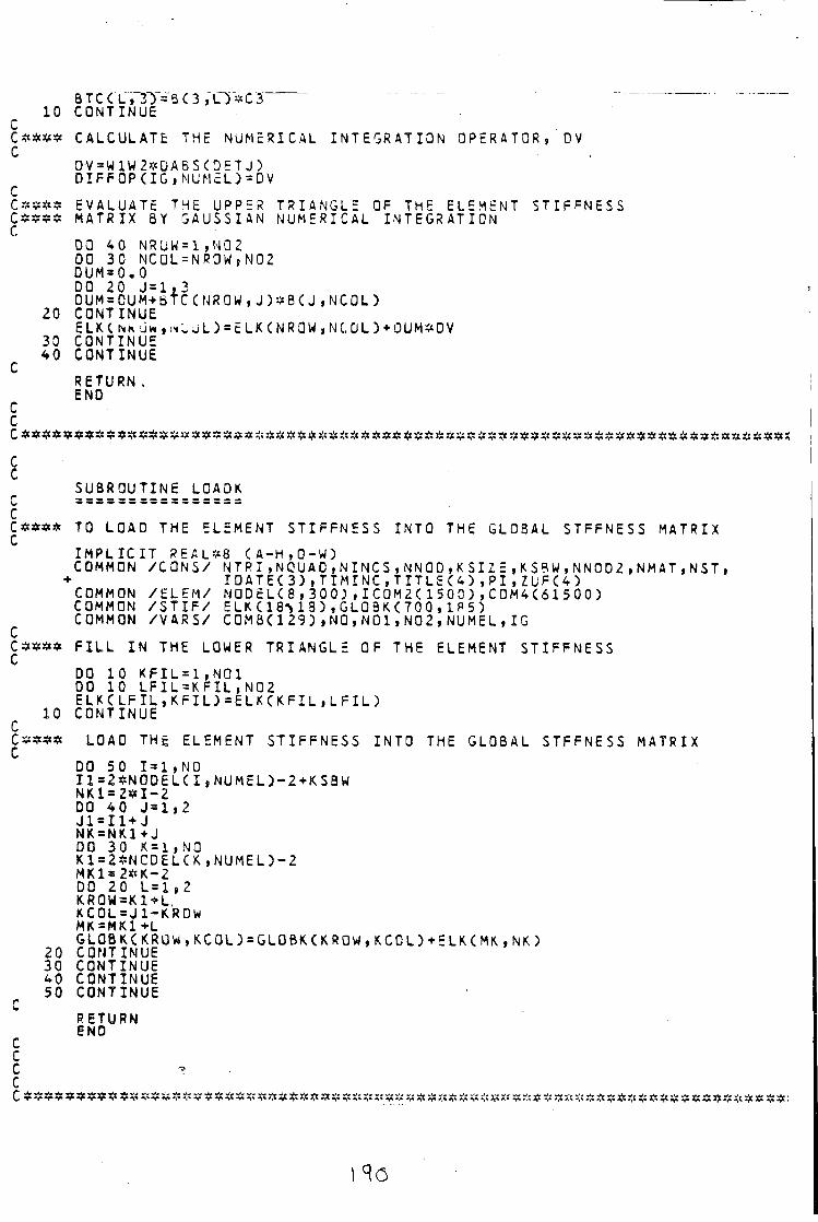
B T C C l , 2 y = & C 3 , L ) * C 3 10 CONTINUE
C * * « * CALCULATE THE NUMERICAL INTEGRATION OPERATOR, DV C
DV=W1W2*DA5S(DETJ) D IFFOP( IG,MUMcL)=OV
C C * * * * EVALUATE THE UPPER TRIANGLE OF THE ELEMENT S T I F F N E S S C * * * * MATRIX B Y GAUSSIAN NUMERICAL INTEGRATION C
00 40 NRLiW = l , NO 2 00 30 NCOL=NR0W,N02 DUM=0.0 DO 20 J = l , 3 OUM = OUM+BTC C N R O W , J ) * B ( J , N C O L )
20 CONTINUE ELKC NkUw, * w u L ) = ELK(NRQW ,NC;OL) + OUM*DV
30 CONTINUE 40 CONTINUE
C RETURN . END
C c C * * * * * * * * * * * * * * * ^ * * * * * * * * * * * * * * * * * * * * * * * * * * * * * * * * * * * * * * * * * * * * * * * * * * * * * * * * * C C
SUBROUTINE LOADK U * = - -
C C * * * * TO LOAD THE ELEMENT S T I F F N E S S INTO THE GL03AL STFFNES5 MATRIX
I M P L I C I T REALMS ( A - H . O - W ) COMMON / C O N S / NTR I ,NQUAD,N INCS,NN0D,KS IZE ,KSBW,NNO02 ,NMAT,NST ,
• I D A T E C 3 ) , T I M I N C , T I T L E ( 4 ) , P I , Z U F C 4 ) COMMON / E L EM/ NODELC8 , 3 0 0 ) , I COM 2( 1 5 0 0 ) , C 0 M 4 C 6 1 5 0 0 ) COMMON / S T I F / ELK ( 1 8 M 8 ) , GLO BK ( 70 0 , 1 8 5 ) COMMON / V A R S / COMB(129) , NO,NO 1,NO 2 ,NUMEL, IG
C * * * * F I L L IN THE LOWER TRIANGLE OF THE ELEMENT S T I F F N E S S
DO 10 KFIL=1 ,M01 DO 10 L F I L = K F I L , N 0 2 E L K ( L F I L » K F I L ) = E L K ( K F I L » L F I L )
10 CONTINUE C C * * * * LOAD THE ELEMENT S T I F F N E S S INTO THE GLOBAL STFFNESS MATRIX
DO 50 1=1,NO 11*2*NODEL( I ,NUMEL3-2+KSBW NK1= 2 * 1 - 2 DO 40 J = l , 2 J1 = I 1 + J NK=NK1+J DO 30 K=1,N0 K1 = 2 *NCDEL(K. ,NUMEL) -2 MK1 = 2 * K - 2 DO 20 L = l , 2 KR0W = K1 + L, KCOL=J 1-K.R0W MK=MK1+L GLQBK(KRGW,KCQL) = GLOBK(KROW,KCOL)+ELK(MK»NK.)
20 CONTINUE 30 CONTINUE 40 CONTINUE 50 CONTINUE
r RETURN END
C C c <? . c C * * * * * * * * * * * * * * * * * * * * * * * * * * * * * * * * * * * * * * * * * * * * * * * * * * * * * * * ^
I S O
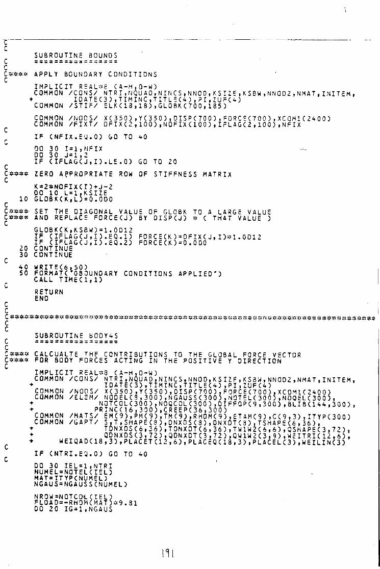
c SUBROUTINE BOUNDS C ================= c C * $ * s APPLY BOUNDARY CONDITIONS C I M P L I C I T REALMS CA-H.O-W)
COMMON / C O N S / N T R I , N Q U A 0 , N I N C S , N N 0 D , K S I Z E , K S B W , N N 0 D 2 , N M A T , I N I T E M , • I D A T E ( 3 ) , T I M I N C , T I T L E D ) , P I , Z U F < 4 )
COMMON / S T I F / E L K ( 1 8 , 1 8 ) , G L O B K C 7 0 0 , 1 8 5 ) COMMON / N O D S / XC 350 ) , Y (350 ) , D I S P C 700 ) , F 0 R C E C 7 0 0 ) ,XCOM1C2400) COMMON / F I X T / 0 F I X<2 , 100) , N 0 F I X ( 1 0 0 ) , I F L A G C 2 , 1 0 0 ) , N F I X
I F C N F I X . E Q . O ) GO TO ^0 DO 3 0 I=1 ,MFIX DO 30 J = l , 2 I F C I F L A G C J . D . L E . O ) GO TO 20
C C # $ # * ZERO APPROPRIATE ROW OF S T I F F N E S S MATRIX
K = 2 * N 0 F l X ( I ) + J - 2 00 10 L = 1 , K S I Z E
10 G L O B K ( K , L 5 = 0 . 0 D 0 C C * * * « SET THE DIAGONAL VALUE OF GLQBK TO A LARGE VALUE
AND REPLACE F O R C E C J ) BY D I S P C J ) * C THAT VALUE )
GL0BKCK,KSBW)=1 .0D12 I F C I F L A G C J i D . E Q . l ) FO R C E ( K ) = OF IX C J , I ) * 1. 0 Dl 2 I F < I F L A G C J , I ) . E Q . 2 ) FORCECK) = 0 .0 DO
20 CONTINUE 30 CONTINUE
C 40 W R I T E C 6 . 5 0 ) 50 FORMATC'OBOUNDARY CONDITIONS A P P L I E D ' )
CALL T I M E < 1 , 1 )
RETURN END
C C C
c SUBROUTINE B0DY4 S
C * * * * CALCUALTE THE CONTRIBUTIONS TO THE GLOBAL FORCE VECTOR FOR BODY FORCES ACTING IN THE P O S I T I V E Y DIRECTION
I M P L I C I T R E A L * 3 ( A - H . O - W ) COMMON / C O N S / NTRI ,NQUAD,N INCS,NN0D,KSIZF ,KSBW,NN0D2 ,NMAT, IN ITEM»
+ I D A T E C 3 ) , T I M I N C , T I T L E C 4 ) , P I , Z U F ( 4 ) COMMON / N O D S / X( 350 ) , YC 350 ) , D I S P ( 7 0 0 ) , F G R C E C 7 0 0 ) ,XC0M1C2400 ) COMMON / E L E M / NOOELC 9 , 300 ) ,NGAUSS( 3005 iNOT E L ( 3005 iNOQELC 300 ) i
• • N O T C 0 L C 3 0 0 ) , N O Q C Q L C 3 0 0 ) , D I F F O P < : 9 > 3 0 0 ) , 3 L I B C 1 4 4 , 3 O 0 ) , + P R I N C C 1 6 , 3 0 0 ) , C R E E P C 3 6 , 3 0 0 )
COMMON / M A T S / E M C 9 ) , P M C 9 ) , T M C 9 ) , R H 0 M ( 9 ) , E T A M < 9 ) , C C 9 , 3 ) , I T Y P ( 3 0 0 ) COMMON / G A P T / S , T , SHAPEC8 ) , 0 N X D S < 3 ) , O N X D T ( 8 ) , T S H A P E ( 6 , 3 6 ) ,
+ T D N X D S ( 6 , 3 6 ) , T 0 N X 0 T C 6 , 3 6 ) , T W 1 W 2 C 6 , 6 ) , Q S H A P E C 3 , 7 2 ) , • Q D N X D S C 3 , 7 2 ) , Q D N X D T ( 3 , 7 2 ) , Q W 1 W 2 ( 3 , 9 ) , W E I T R I C 1 2 , 6 ) , • W E I Q A D C 1 8 , 3 ) , P L A C E T C 1 2 , 6 ) , P L A C E Q C 1 8 , 3 ) , P L A C E L C 3 ) , W E I L I N C 3 )
I F C N T R I . E Q . O ) GO TO 40
DO 30 I E L = 1 , N T R I NUMEL=NOTELCIEL) MAT=ITYPCNUMEL) NGAUS=NGAUSSCNUMEL)
NR0W=N0TCO=L C I E L ) FL0AD=-RH0M(MAT)*9 .31 DO 20 IG=1,NGAUS
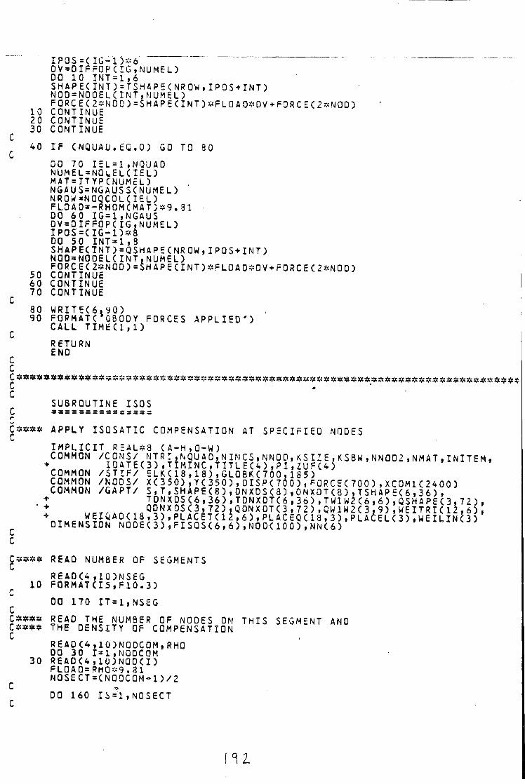
I P O S = C I G - 1 ) * 6 ~~" " " O V = D I F F O P C : G , N U M E L ) DO 10 I N T = 1 , 6 SHAPECINT)=TSHAP5CNR0W, IP0S+INT) N 0 D = N 0 0 E L C I N T , N U M E L ) F 0 R C E C 2 * N 0 D ) = S H A P E C I N T ) * F L 0 A D * D V + F 0 R C E C 2 * N 0 Q )
10 CONTINUE 20 CONTINUE 30 CONTINUE
C 40 I F CNQUAU.EG.O) GO TO 30
00 70 I E L = 1 » NQU A0 NUMEL=NQuELCIEL) MAT=JTYPCNUMEL) NGAUS=NGAUSSCNUMEL) NROW=NOQCOLCIEL) FL0A0»-RH0MCMAT)#9 .31 DO 60 IG=1,NGAUS DV=DIFFOPCIG,NUMEL) I P 0 S = C I G - 1 ) * 8 DO 50 INT=1,8 SHAPECTNT)=QSHAPECNROW,IPOS+INT) NOD=NQDELCINT.NUMEL) F 0 R C E C 2 * N 0 D ) = S H A P E C I N T ) * F L 0 A 0 * 0 V + F 0 R C E C 2 * N 0 D )
50 CONTINUE 60 CONTINUE 70 CONTINUE
C 80 W R I T E C 6 . 9 0 ) 90 FORMATC O B O D Y FORCES A P P L I E D ' )
CALL T I M E C l . l ) RETURN END
r C
c SUBROUTINE ISOS
r
C « * * « APPLY I S O S A T I C COMPENSATION AT S P E C I F I E D NODES
I M P L I C I T R=AL*8 ( A - H . O - W ; COMMON / C O N S / NTRI ,NQUAD,N INCS,NNO 0 , K S I Z E . K S B W , N N 0 0 2 , N M A T , I N I T E M ,
+ I D A T E C 3 ) , T I M I N C , T I T L E C 4 ) , P I , Z U F C 4 ) COMMON / S T I F / E L K C 1 8 . 1 8 ) , G L O B K ( 700 , 185 ) COMMON / N O D S / X C 3 5 0 ) , Y C 3 5 0 ) , D I S P C 7 0 0 ) , F O R C E C 7 0 0 ) , X C O M 1 C 2 4 0 0 ) COMMON / G A P T / S , T , S H A P E C 8 ) , O N X D S C 8 ) , 0 N X O T < 8 ) , T S H A P £ C 6 , 3 6 ) ,
• T D N X D S C 6 , 3 6 ) , T D N X D T C 6 , 3 b ) , T W l W 2 C 6 , 6 ) , Q S H A P E C 3 , 7 2 ) , 1 u = T • Q QDNXDSC3, 72_» , Q DN X DT C 3 , 7 2 ) ,QW1W2C3,9) , W E I T R I ( 1 2 , 6 ) • W E I U A D C 1 8 , 3 ) , P L A C E T C l i , 6 ) , P L A C E Q C 1 8 , 3 ) , P L A C E L C 3 ) , W E I L I N C 3 )
OIMENSION N0DEC3) , F I S 0 S C 6 , 6 ) ,NODC100) ,NNC6) C
READ NUMBER OF SEGMENTS
READC4 , 1 0 ) N S E G 10 F O R M A T C I 5 , F 1 0 . 3 )
DO 170 I T = 1 , N S E G C
READ THE NUMBER OF NODES ON THIS SEGMENT AND C * * # * THE DENSITY OF COMPENSATION
REA0C4,10)N0DC0M,RH0 DO 30 I=1,N0DC0M
30 REA0C4 , 1 0 ) N 0 D C I ) FL0A0=RHQ*9 .81 N0SECT=CN0DC0M- l ) / 2
DO 160 I S = 1 , N 0 S E C T
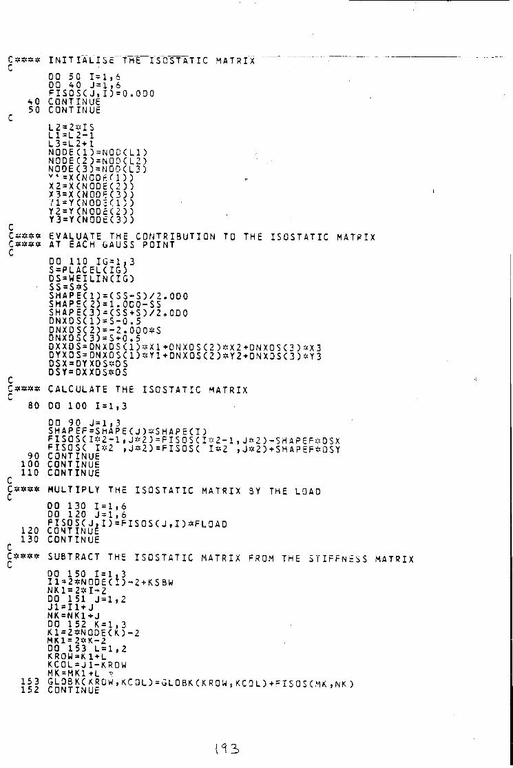
C « * * * I N I T I A L I S E THE I S O S T A T I C MATRIX
40 50
C
C
00 50 1=1,6 00 40 J = l , 6 F I S O S C J , I ) = 0 CONTINUE CONTINUE
000
L 2 = 2 * I S L 1 = L 2 - 1 L3=L2+1 N0DEC1)=N0DCL1) N0DEC2)=N0DCL2) NODE C3) = N0QCL3) v " =X(NOOr.n )) X2=XCNOOEC2)) X3 = X CN0DEC3)) V l = Y ( N 0 0 c C n ) Y2=YCN00cC2) ) Y3=YCN0DtC3) )
EVALUATE THE AT EACH GAUSS
CONTRIBUTION POINT
TO THE I S O S T A T I C MATRIX
00 110 I G = 1 , 3 S = P L A C E L C I G ) D S = W E I L I N C I G ) S S = S * S S H A P E C l ) = C S S - S ) / 2 . O D O S H A P E C 2 ) = 1 . 0 D 0 - S S S H A P E C 3 ) = C S S + S ) / 2 . 0 D 0 D N X O S C l ) = S - 0 . 5 DNXDSC 2) = - 2 . 0 0 0 * S DNX0SC3)=S+0.5 0XX0S=DNXDSC1)*X1>0NX0SC2)*X2+ONXOSC3)*X3 OYXOS=DNXOSC1)*Y1+DNXOSC2)*Y2+DNXQSC3)*Y3 OSX=OYXOS*DS DSY=DXXOS*OS
<* CALCULATE THE I S O S T A T I C MATRIX
00 100 1=1 ,3
DO 90 J = l , 3 S H A P E F = S H A P E C J ) - S H A P E C I ) F I S O S C 1 * 2 - 1 , J * 2 ) = F I S 0 S C 1 * 2 - 1 , J * 2 ) - S H A P E F * Q S X F I S O S C 1*2 , J * 2 ) = F I S 0 S C 1*2 , J * 2 ) + SHAPEF*DSY
90 CONTINUE 100 CONTINUE 110 CONTINUE
MULTIPLY THE I S O S T A T I C MATRIX BY THE LOAD DO 130 1=1 ,6 DO 120 J = l , 6 F I S O S C J , I ) = F I S O S C J , I ) * F L O A O CONTINUE CONTINUE
SUBTRACT THE I S O S T A T I C MATRIX FROM THE S T I F F N E S S MATRIX DO 150 1=1 ,3 I l = 2 * N 0 D E C I ) - 2 + K S B W N K l = 2 * I - 2 DO 151 J = l , 2 J1 = 11 + J NK=NK1+J DO 152 K = l , 3 K1=2*N0DECK)=2 MK1= 2 * K - 2 DO 153 L = l , 2 KROW=K1+L KCOL = J 1-K.ROW MK=MK1+L *
153 GLOBKCKROW,KCOL) = GLOBKCKROW,KCOL)-t-FISQSCMK,NK) 152 CONTINUE
H2>
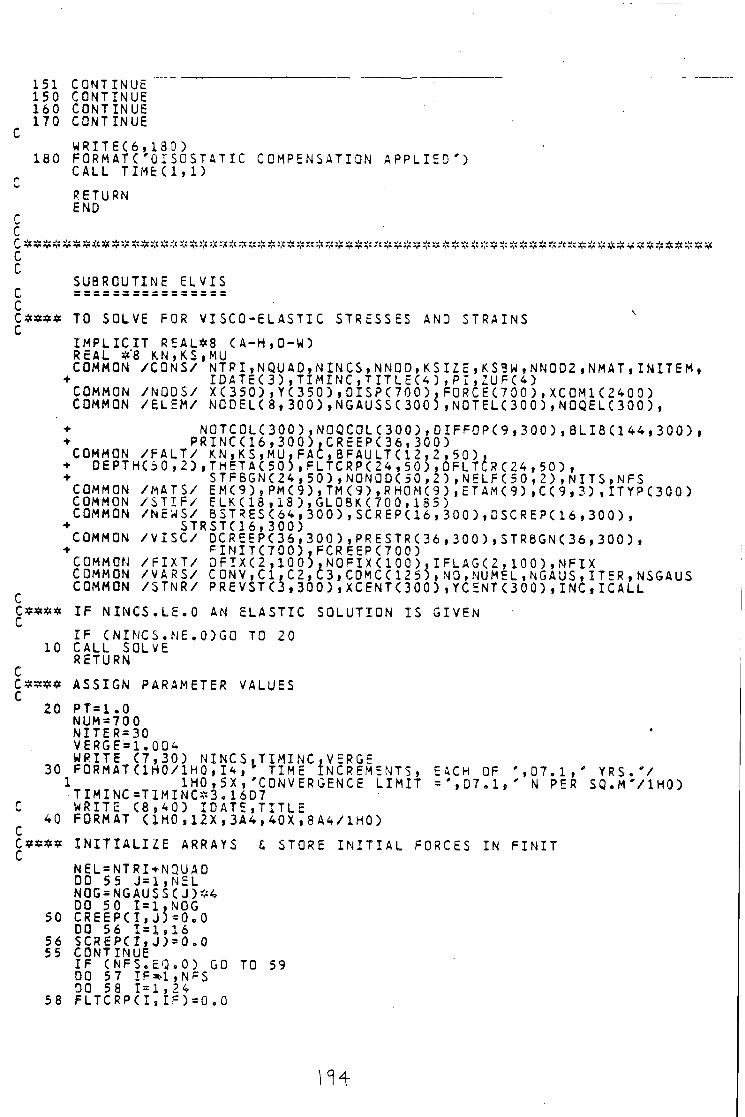
151 150 160 170
180
CONTINUE CONTINUE CONT INUE CONT INUE
W R I T E C 6 , FORMAT C '
180 ) O ISOSTATIC COMPENSATION A P P L I E D ' )
CALL T I M E ( 1 , 1 )
RETURN END
C C C C
C C Csas* C
SUBROUTINE E L V I S
TO SOLVE FOR V I S C 0 - E L A S T I C S T R E S S E S AND STRAINS
I M P L I C I T R E A L * 8 CA-H ,0 -W) REAL *'8 K.N,KS,MU COMMON / C O N S / NTP I ,NQUAD,N INCS,NNQD,KS IZE ,KS3W,NN002 ,NMAT, IN ITEM,
+ I D A T E < 3 ) , T I M I N C , T I T L E C 4 ) , P I , Z U F ( 4 ) COMMON / N O D S / XC350) , Y C 3 5 0 ) , 0 1 S P C 7 0 0 ) , FORCEC700 ) , X C O M 1 ( 2 4 0 0 ) COMMON / E L EM/ NODELC 8 , 3 0 0 ) , N G A U S S C 3 0 0 ) , N O T E L C 3 0 0 ) , N O Q E L C 3 0 0 ) ,
C
C
10
N O T C O L C 3 0 0 ) , N O Q C O L C 3 0 0 ) , D I F F a P C 9 , 3 0 0 ) , 8 L I B C l 4 4 , 3 0 0 ) . P R I N C ( 1 6 , 3 0 0 ) . C R E E P ( 3 6 , 3 0 0 )
COMMON / F A L T / KN,KS,MU,FAC,BFAULT(12,2,50), C 5 0 , 2 ) , T H E T A C 5 0 ) , F L T C R P C 2 4 , 5 0 ) , D F L T C R C 2 4 , 5 0 ) ,
STFBGNC24 , 5 0 ) , N O N 0 D C 5 0 , 2 ) , N E L F C 5 0 , 2 ) , N I T S , N F S / M A T S / E M < 9 ) , P M < 9 ) , T M ( 9 ) , R H 0 M C 9 ) , E T A M ( 9 ) , C ( 9 , 3 ) , I T Y P ( 3 0 0 ) / S T I F / E L K C 1 8 , 1 8 ) , G L O B K C 7 0 0 , 1 3 5 ) / N E W S / B S T R E S C 6 4 , 3 0 0 ) , S C R E P ( 1 6 , 3 0 0 ) , D S C R E P C 1 6 , 3 0 0 ) ,
S T R S T C 1 6 , 3 0 0 ) COMMON / V I S C / 0 C R E E P ( 3 6 , 3 0 0 ) , P R E S T R ( 3 6 , 3 0 0 ) , S T R 8 G N < 3 6 , 3 0 0 ) ,
F I N I T C 7 0 0 ) , F C R E E P C 7 0 0 ) / F I X T / O F I X C 2 , 1 0 0 ) . N a P I X C 1 0 0 ) , I F L A G ( 2 , 1 0 0 ) , N F I X / V A R S / C O N V , C 1 , C 2 , C 3 , C O M C ( 1 2 5 ) , N O , N U M E L , N G A U S , I T E R , N S G A U S / S T N R / P R E V S T C 3 , 3 0 0 ) , X C E N T ( 3 0 0 ) , Y C E N T C 3 0 0 ) , I N C , I C A L L
I F N I N C S . L E . O AN E L A S T I C SOLUTION I S GIVEN
+ O E P T H C 5 0 . 2 ) +
COMMON COMMON COMMON
+
COMMON COMMON COMMON
I F ( N I N C S . N E . O ) G O TO 20 CALL SOLVE RETURN
:* ASSIGN PARAMETER VALUES
2 0
30
C 40
C C$<:#* C
50
56 55
58
EACH OF = ' , 0 7 . 1 ,
PT=1 .0 NUM=700 NITER=30 V E R G E a l . 0 0 4 WRITE C 7 , 3 0 ) N I N C S , T I M I N G . V E R G E FORMATC1H0/1H0,14 , 1 TIME INCREMENTS,
1H0,5X , 'CONVERGENCE L IMIT T IMINC=TIMINC*3 .16D7 WRITE ( 8 , 4 0 ) ID A T E , T I T L E FORMAT C 1 H 0 , 1 2 X , 3 A 4 , 4 0 X , 8 A 4 / 1 H 0 )
I N I T I A L I Z E ARRAYS I STORE I N I T I A L FORCES IN F I N I T
NEL=NTRI+N3UAD DO 55 J = 1 , N E L NOG=NGAUSSCJ)*4 DO 50 I=1,N0G C R E E P C I i J ) = O o O DO 56 1=1 ,16 S C R E P C I i J ) = 0 . 0 CONTINUE I F C N F S . E Q . O ) GO TO 59 DO 57 IF=*1,NFS DO 58 1=1,24 F L T C R P C I , I F ) = 0 . 0
, 0 7 . 1 , ' YRS . ' / N PER S Q . M ' / I H O )
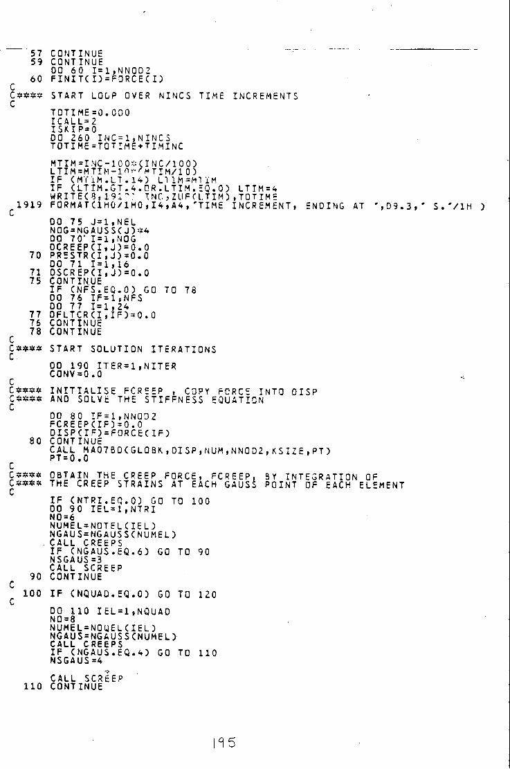
57 CONTINUE 59 CONTINUE
DO 60 I=1,NN0D2 60 F I N I T C I ) = F O R C E C I ) C
C 3 * * $ START LOOP OVER NINCS TIME INCREMENTS C
TOTIME =0.ODO ICALL=2 I S K I P = 0 DO 260 INC=1»NINCS TOTIME=TOTIME+TlMINC
M T I M = I N C - 1 0 0 * ( I N C / 1 0 0 ) LTIM=MTIM-inv-/-MTlM/l 0) I F C MT i M . L T . 1 4 ) LUM=M*tiM I F ( L T I M . G T . 4 . O R . L T I M . E Q . 0 ) LTTM=4 W R I T E C 3 S 1 9 1 " " INC , ZUF C L TIM ) , TOT IM E
^1919 F O R M A T ( 1 H 0 / 1 H 0 » I 4 » A 4 , 'T IME INCREMENT, ENDING AT ' , 0 9 . 3 , ' S . V 1 H )
DO 75 J = 1 , N E L NOG=NGAUSS(J)*4 DO 70* 1 = 1,NOG D C R E E P C I , J ) = 0 . 0
70 P R E S T R C I , J ) = 0 . 0 DO 71 1=1 ,16
71 D S C R E P C I , J ) = 0 . 0 75 CONTINUE
I F ( N F S . E Q . O ) GO TO 78 DO 76 I F = 1 , N F S DO 77 1=1,24
77 D F L T C R ( I , I F ) = 0 . 0 76 CONTINUE 78 CONTINUE C
C * * # # START SOLUTION ITERATIONS DO 190 ITER = 1 , N I T E R CONV=0.0
C * * $ * I N I T I A L I S E FCREEP , COPY FORCE INTO DISP C * * « * AND SOLVE THE S T I F F N E S S EQUATION
DO 80 IF=1,NN0D2 F C R E E P C I F ) = 0 . 0 D I S P ( I F ) = F O R C E ( I F )
80 CONTINUE CALL M A 0 7 B D ( G L O B K , D I S P , N U M f N N O D 2 , K S I Z E , P T ) PT = 0 .0 C
C * S * * OBTAIN THE CREEP FORCE, F C R E E P . BY INTEGRATION OF C * * $ * THE CREEP STRAINS AT EACH GAUSS POINT OF EACH ELEMENT C
I F C N T R I . E Q . O ) GO TO 100 DO 90 I E L = 1 , N T R I N0=6 NUMEL=NOTEL( IEL) NGAUS=NGAUSS(NUMEL)
. CALL CREEPS I F C N G A U S . E Q . 6 ) GO TO 90 NSGAUS=3 CALL SCREEP
90 CONTINUE C
100 I F CNQUAO.EQ.O) GO TO 120
DO 110 I E L = 1 ,NQUAD NO = 8 NUMEL=NOQELCIEL) NGAUS=NGAUSS(NUMEL) CALL CREEPS I F ( N G A U S . E Q . 4 ) GO TO 110 NSGAUS=4
CALL SCREEP 110 CONTINUE
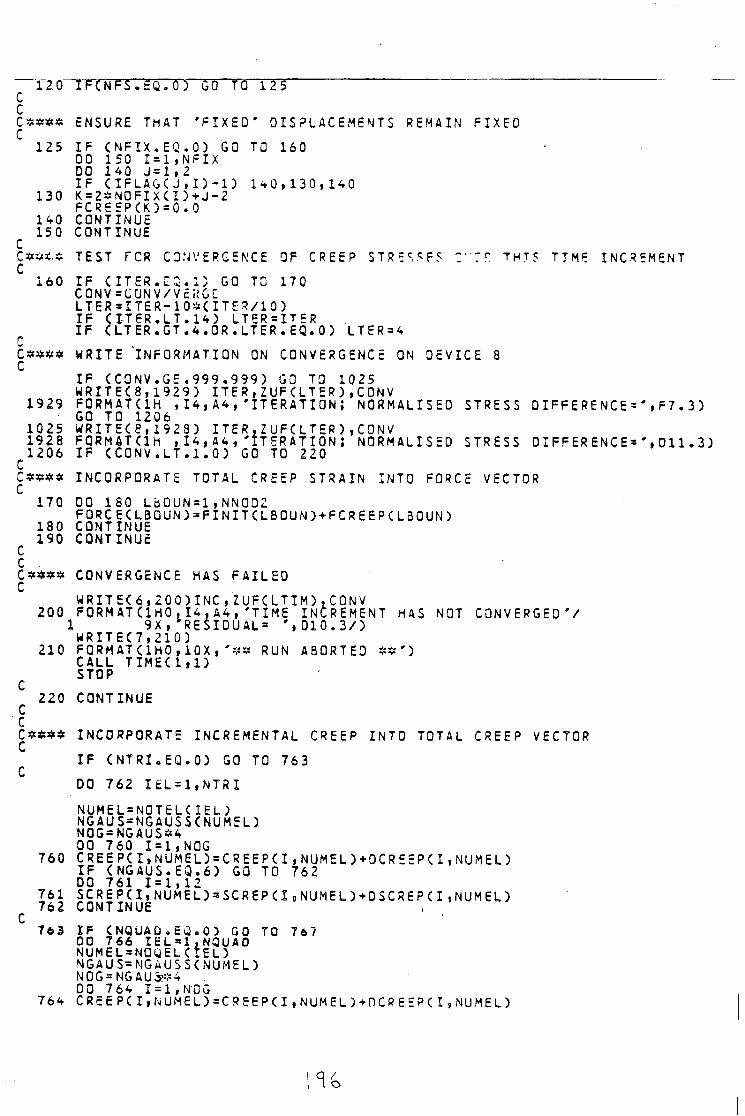
r Z O ^ F C N P S . S Q . O ) GO TQ 125 c c C * * $ * ENSURE TMAT ' F I X E D ' DISPLACEMENTS REMAIN F I X E D C
125 I F C N F I X . E Q . O ) GQ TO 160 DO 150 I = 1 , N F I X DO 140 J = l , 2 I F C I F L A G C J , I ) - l ) 1 * 0 , 1 3 0 , 1 4 0
130 K = 2 * N O F l X C I ) + J - 2 F C R E E P C K ) = 0 . 0
140 CONTINUE 150 CONTINUE
C C * * * . * TEST FCR CONVERGENCE OF CREEP S T R E C , ^ F 5 2' T r THIS TIME INCREMENT C
160 I F C I T E R . E Q . l ) GO TO 170 CONVsCONV/VcliCi: L T E R = I T E R - 1 0 * C I T E R / 1 0 ) I F C I - T E R . L T . 14) L T E R = I T E R I F C L T E R . G T . 4 . 0 R . L T E R . E Q . O ) LTER=4
C * S # $ WRITE 'INFORMATION ON CONVERGENCE ON DEVICE 8 C
I F C C O N V . G E . 9 9 9 . 9 9 9 ) GO TO 1025 W R I T E C 8 , 1 9 2 9 ) I T E R , Z U F C L T E R ) , C O N V
1929 FORM AT C1H , 14 , A4 , ' I T E R A T I 0N; NORMALISED STRESS D I F F E R E N C E = ' , F 7 . 3 ) GO TO 1206
1025 W R I T E C 8 , 1 9 2 8 ) I T E R , Z U F C L T E R ) , C 0 N V 1928 FORMAT CIH , 1 4 , A 4 , ' I T E R A T I 0N; NORMALISED STRESS D I F F E R E N C E S ' , O i l . 3 ) 1206 I F C C O N V . L T . 1 . 0 ) GO TO 220
C C#s#* INCORPORATE TOTAL CREEP STRAIN INTO FORCE VECTOR C
170 00 180 LbOUN=l,NN0D2 FORC ECLBQUN)=FIN ITCLB0UN) + FCREEPCL3QUN)
180 CONTINUE 190 CONTINUE
C c . C * * * $ CONVERGENCE HAS F A I L E D C
W R I T E C 6 , 2 0 0 ) I N C , Z U F C L T I M ) , C 0 N V 200 F 0 R M A T C 1 H 0 , I 4 . A 4 , 'T IME INCREMENT HAS NOT CONVERGED' /
1 9X , l R E S I O U A L = ' , D 1 0 . 3 / ) W R I T E C 7 , 2 1 0 )
210 FORMATC1HO,10X,' - ,<* RUN ABORTED * * ' ) CALL T I M E C 1 , 1 ) STOP
C 220 CONTINUE
C ' C
C * * * * INCORPORATE INCREMENTAL CREEP INTO TOTAL CREEP VECTOR
I F C N T R I . E Q . O ) GO TO 763 C
DO 762 I t L = l , N T R I NUMEL=NOTELCIEL) NGAUS=NGAUSSCNUMEL) N0G=NGAUS=*4 00 760 1=1,NOG
760 C R E E P C I , N U M E L ) = C R E E P C I , N U M E L ) + D C R E 5 P C I , N U M E L ) I F CNGAUS.EQ.6 ) GO TO 762 DO 761 1 = 1 , 1 2
761 S C R E P ( I , N U M E L ) = S C R E P C I 8 N U M E L )+ DSCREPCI 9 NUMEL) 762 CONTINUE
C 763 IP CNQUAO.EQ.O) GQ TQ 767
DO 766 IEL»1 ,NQUA0 NUMEL=NOQELCIEL) NGAUS=MGAUSSCNUMEL) N0G = NGAUJ?*4 DO 764 1 = 1 , N O G
764 C R E E P ( I , N U M E L ) = C R E E P ( I , N U M E L ) + 0 C P E 5 P ( I , N U M E L )
I F CNGAU 3 • E Q . 4 ) GO TO 76 6 DO 765 1 = 1 , 1 6
76 5 SCREPCI ,NUMED=SCREPCI» NUM 6 L ) + OSCREPCI,NUMEL) 766 CONTINUE
C 767 I F CNFS.EQ.O) GO TO 770
OQ 769 I F = 1 , N F S DO 768 1 = 1 , 2 4
76 9 F L T C R P C I , I F ) = F L T C R P C I , I F ) + D F L T C R C I , I F ) 769 CONTINUE 770 CONTINUE
C C $ * s * SET UP FORCE VECTORS FOR NEXT TIME INCREMENT
DO 240 NEXTF=1,NNHD2 F IN ITCNEXTF) = F I N I H N E X T F ) + FCREEPCNEXTF) F O R C E ( N E X T F ) = F I N I T ( N E X T F )
240 CONTINUE W R I T E C 6 . 2 5 0 ) I N C , 2 U F ( L T I M )
250 F O R M A T C 1 H O , I 4 . A 4 , ' T I M E INCREMENT COMPLETE * ) CALL T I M E ( l , l 5
C r
260 CONTINUE T I M I N C = T I M I N C / 3 . 1 6 0 7
RETURN END
C SUBROUTINE SOLVE
C C * « * * SOLVE THE STIFFNESS EQUATION
I M P L I C I T REALS8 CA-H.O-W) REALS8 KN,KS.MU COMMON /CONS/ N T R I , N Q U A 0 , N I N C S , N N Q D , K S I 2E , KSBW,NNOD2,NMAT, IN ITEM {
+ IDATEC3) , T I M I N C , T I T L E C 4 ) , P I , Z U F < 4 ) COMMON /NODS/ X ( 3 5 0 ) , Y<350 ) , D I S P C 7 0 0 ) . F O R C F C 7 0 0 ) , X C 0 M 1 ( 2 4 0 0 ) COMMON / F A L T / KN , K S , M U , F A C , B F A U L T C 1 2 , 2 , 5 0 ) ,
+ D E P T H C 5 0 , 2 ) , T H E T A C 5 0 ) , F L T C R P C 2 4 , 5 0 ) . D F L T C R ( 2 4 f 5 0 ) , • S T F B G N C 2 4 , 5 0 ) , N O N O D C 5 0 , 2 ) , N E L F C 5 0 , 2 ) , N I T S , N F S
COMMON / S T I F / ELKCI 8 , 1 8 ) , G L 0 B K C 7 0 0 , 185 ) COMMON / E L EM/ NOD EL (8 i 300 ) ,NGAUSS( 3 0 0 ) , NOTELC300)•NOQELC300 ) f
+ N O T C O L C 3 0 0 ) , N O Q C O L C 3 0 0 ) , D I F F O P C 9 f 3 0 0 ) , B L I B C 1 4 4 9 3 0 0 ) , • P R I N C C 1 6 , 3 0 0 ) , C R E E P C 3 6 , 3 0 0 )
c C $ * * * COPY FORCE INTO DISP AND SOLVE THE STIFFNESS EQUATION
00 10 I=1 ,MN0D2 10 O I S P C I ) = F O R C E C I )
C
c
NUM=700 PT = 1 . 0 CALL MA0 7BDCGL0 3 K » D I S P , N U M , N N 0 D 2 , K S I 2 E . P T )
15 W R I T E C 7 . 2 0 ) 20 FORMAT CI HO,1 OX» 'ELASTIC A N A L Y S I S ' )
W R I T E C 6 . 3 0 ) 30 FORMATC ' 0 EQUATION SOLVED ' )
CALL T I M c C l n l ) RETURN END
C C * * * $ $ # # * * * £ * £ : < : * * * * # # * * * * # : ^
C SUBROUTINE STRESS
c c c
+ / H A T S / I T Y P C 3 0 0 ) /NEWS/
STRSTC16 / G A P T / HAPEC6
c
6 1001
7 c c
5 10
c c * * # * c
30
c
50
CALCULATE THE STRESS AT EACH GAUSS POINT
I M P L I C I T PEALS8 < A - H , 0 - W ) COMMON /CONS/ N T R I , N Q U A 0 , N I N C S , N N 0 Q , K S I Z E , K S 8 W , N - N 0 D 2 , N M A T , I N I T E M ,
y I D A T E C 3 ) i S T M A X , T I T L E C 4 ) , P I , Z U F C 4 ) COMMON /NODS/ X ( 3 5 0 ) , Y C 3 5 0 ) , O I S P C 7 0 0 ) , F Q R C e < 7 0 0 ) , X S T P O S ( 4 , 3 0 0 ) ,
• Y S T P D S < 4 , 3 0 0 ) COMMON / t L 5 M / N 0 0 E L C 8 , 3 0 0 D . N G AU S S C 3 0 0 ) . NO T = L C 3 0 0 1 . N 00 E L ( 3 0 0 1 .
h COMMON COMMON
COMMON
WEIQADC18 COMMON / V A R S /
I F C N T R I . E Q . 0 ) G O TO 70 N0=6
START TO EVALUATE THE STRESS IN TRIANGULAR ELEMENTS
DO 60 I E L = 1 | N T R I
NUMEL=NOTEL( IEL) MAT=ITYPCNUMEL) NGAUS=NGAUSS(NUMEL) C1=CCMAT,1) C2=CCMAT,2) C 3 = C ( M A T , 3 ) I F CNGAUS.NE.6) GO TO 5 I F CNINCS.EQ.O) GO TO 1001 00 6 I S = 1 , 1 2 SCREP<IS,NUMEO=CREEP<12 + I S , N U M E L ) 00 7 I U » 1 ; 3 6 BSTRESCIS f NUMEL) = 3L IBC36 + IS ,NUMEL)
UNLOAD THE DISPLACEMENTS FOR THIS ELEMENT
00 10 J = l , 6 Q C 2 * J - 1 ) = D I S P < 2 # N 0 D E L ( J , N U M E L ) - 1 ) Q( 2 * J )=DISPC 2SN0DELCJ,NUMEL} 5 CONTINUE CALCULATE THE POSITION AN0 RECALL THE STRAIN MATRIX FOR EACH GAUSS POINT AT WHICH STRESS IS TO 8E COMPUTED
DO 50 I G = 1 , 3 I P 0 S = C I G + 2 ) * 6 K P O S = C I G - 1 ) # 1 2 XPOS=0.0 YPOS=0.0 DO 30 I V = 1 , N 0 S H A P E C I V ) = T S H A P E C l f I P O S + I V ) NOD=NODELf IV,NUM£L) XP0S=XPOS+SHAPECIV)*X(NOD) YPOS=YPOS+SHAPECIV)^YCNOD) L = 2 * I V K = L - 1 DNXDXCIV)=3STRESCKP0S+K,NUMEL) ONXOYCIV)=SSTRES(KPQS+LjNUMEL) CONTINUE
XSTPOSCIG,NUMEL)=XPOS YSTPOSCIG 9NUMEL)=YPOS
EVALUATE THE PRINCIPAL STRESSES
CALL PRIt iCS
CONTINUE
60 CONTINUE C C * # # * START TO EVALUATE STRESSES IN QUADRILATERAL ELEMENTS
70 I F(N QU AD.E Q . 0 ) G O TO 140 NO = 8 DO 130 I E L = 1iNQUAD NUMEL=N0UEL( I5L ) NGAUS=NGAUSS(NUMEL) MAT=ITYP(NUMEL) C l = C ( M A T , l ) C2 = C CHAT,2) C 3 = C ( M A T , 3 )
I F <NG4 'JS .NE.4 ) GO TO 7 9 I F ( N I N C S . E Q . O ) GO TO 1000 DO 71 IS = 1 j 16
71 SCREPCIS ,NUMEL)=CREEP<:iS i N U J T . : 1000 DO 72 I S = 1 , 6 4
72 B S T R E S C I S , N U M E L ) = 3 L I 8 C I S , N U H E L )
C * * * * UNLOAD THE DISPLACEMENTS FOR THIS ELEMENT C
79 00 8 0 J = l , N O Q < 2 * J - l ) = D I S P < 2 * N 0 D E L ( J i N U M E L D - l ) QC 2 * J )=D ISP< 2*NODEL(J .NUMEL) )
80 CONTINUE r C S S * * CALCULATE THE POSITION AND RECALL THE STRAIN MATRIX C#=*#* FOR EACH GAUSS POINT AT WHICH STRESS IS TO SE COMPUTED C
DO 120 IG = 1 , 4 I P O S = C I G - l ) * N O KPOS=IPOS*2 XPOS=0 .0 YPOS = 0 . 0 00 100 I V = l , N O J P 0 S = I P 0 S + I V SHAPECIV)=QSHAPEC1,JP0S) NOD=NOOELCIV,NUMEL) XPOS=XPOS+SHAPE( IV)*X(NOD) YPOS=YPOS+SHAPE<IV)*Y(NOD) L = 2 * I V K = L- 1 DNXDX( IV)=3STRESCKP0S*K,NUMEL) DNXDY(IV)=BSTRESCKPOS+L,NUMEL)
100 CONTINUE XSTPOS CIG,NUMEL)=XPOS YSTPOS(IG,NUMEL)=YPOS
C C * * s * EVALUATE THE PRINCIPAL STRESSES
CALL PRINCS 120 CONTINUE 130 CONTINUE *
C 140 W R I T E ( 6 , 1 5 0 )
150 FORMATC'OPRINCIPAL STRESSES COMPUTED ' ) CALL T I M E C l i l ) RETURN END
C C C * * * * * * * * * * * * * * * * * * * * * * * * 3 * * * : « s $ 3 * $ : { s $ 3 * : f c ^ c C
SUBROUTINE PRINCS
C * * * * CALCULATE THE PRINCIPAL STRESSES
I M P L I C I T R5AL*8 C A - H , 0 - W ) REAL * 8 f L A C E T , PLACEQ
COMMON /CONS/ N T R I , N Q U A D , N I N C S , N N O D , K S I Z E , K S E W f N N O D 2 , N M A T , I N I T E M ,
m
COMMON / fc L E M / N O D E L ( 8 , 3 0 0 ) , N G A U S S ( 3 0 0 5 , N O T 5 l < 3 0 0 ) , N O v 3 = L ( 3 0 0 ) , N O T C O L < 3 0 0 ) , N O Q C a L C 3 0 0 ) , O I F F a P C 9 , 3 0 0 ) , B L I B ( 1 4 4 t 3 0 0 )
P R I N C C 1 6 , 3 0 0 ) , C R E E P C 3 6 , 3 0 0 ) COMMON / M A T S / E M C 9 ) , P M < 9 ) , T M ( 9 ) , R H O M ( 9 ) , E T A M ( 9 ) , C C 9 , 3 ) , I T Y P < 3 0 0 ) COMMON / N E w S / 3 S T R E S ( 6 4 , 3 0 0 ) , S C R E P C 1 6 , 3 0 0 ) , 0 S C R E P.C 1 6 , 3 0 0 ) »
S T R S T C 1 6 , 3 0 0 ) / V A 3 S / C 0 < 2 ) , C 1 , C 2 , C 3 , D N X D X ( 3 ) , D N X D Y ( S ) , Q C 1 3 ) , S T R N ( 4 ) ,
STRESC4) ,C0M11C82) ,N0 ,MUMEL,NGAUS.MAT, IG COMMON / G A P T / S , T , S H A P E C 8 ) , O N X 0 S ( 8 ) , D N X O T ( 8 ) , T S H A P E C 6 , 3 6 ) ,
T D N X D S ( 6 , 3 6 ) , T Q N X D T ( 6 , 3 6 ) , T W 1 W 2 ( 6 , 6 ) , Q S H A P E C 3 , 7 2 ) , Q D N X D S ( 3 , 7 2 ) , Q O N X 0 T ( 3 , 7 2 ) , Q W l U 2 ( 3 , 9 ) , C 0 M 2 ( 2 5 3 ) S T R 0 ( 4 , 3 5 0 ) , C F A I L C 4 , 3 0 0 ) , F A N G L ( 4 , 3 0 0 ) , I F A I L ( 4 , 3 0 0 )
COMMON
COMMON / F A L E /
E = EM CM AT) P = PM CMAT) STRN(1 ) = 0,
S T R N C 3 ) = 0 , S T R N < 4 ) = 0
C**ift E V A L U A T E THE NON-ZERO COMPONENTS OF S T R A I N , S T R N = ( B ) ( Q )
l N 0 E X = a . G - l ) * 4 DO 10 1=1,NO L = 2 * I K = L - 1 S T R N C l ) = S T R N ( l ) + O N X O X ( I ) f t Q C K ) S T R N C 2 ) = S T R r K 2 ) + 0 N X D Y C I ) * Q C L ) S T R N ( 3 ) = S T R N C 3 ) + D N X D X C I ) * 3 C L ) + D N X D Y C I ) * Q ( K )
10 CONTINUE C
I F ( I N I T E M . E Q . O ) G O TO 150
C s s * * CALCULATE I N I T I A L STRAINS I F A TEMPERATURE ANOMALY IS PRESENT ST0X=0 .0D0 ST0Y=O . 0 0 0 STOXY=0.000 S T 0 Z = 0 . 0 D 0
C I F ( N 0 . E Q . 8 ) GO TO 100 I P O S = C I G + 2 ) * N 0 00 90 1=1,NO NOD=NOOEL(I ,NUMEL) SHAP=TSHAPEC1 , IPOS* I ) STOX = STOX + ShAP*STROC 1,NOD) STOY=STOY+SHAP*STR0(2,NOD)
90 ST0XY=STOXY>SHAP*STR0(3,NOO) GO T O 110
C 100 I P 0 S = C I G - 1 ) * N 0
D O 120 1 = 1 , NO NOO=NODELCI ,NUMEL) S H A P = Q S H A P E ( 1 , I P 0 S + I ) ST0X=ST0X+SHAP#STR0C1,N0D) ST0Y=ST0Y+SHAP*STR0(2 ,NOD)
120 ST0XY=STQXY+SHAP*STR0(3,NOD)
110 STRNC1 ) = STRN<1) -ST0X S T R N ( 2 ) = S T R N ( 2 ) - S T 0 Y STRNC3 )=STRN<3) -ST0XY S T R N ( 4 ) = - S T Q X / 1 . 2 5
150 CONTINUE C
I F (NINCSoEQoO)GO TO 30 DO 20 1 = 1 , 4
20 STRNCI )=STRN<I ) -SCREP< I -HNOEX 9 NUMEL) 30 STRNC1)=STRNC1)+P*STRNC4)
STRN<2)=STRN(2 )+P*STRNC4)
FORM STRESSES FROM STRAINS
STRES(1)=C1^STRNC1)+C2-STRNC2)
2 0 0
STRETC2~) = C~2*STRhCl") + C l *STRN( :21 S T R E S C 3 ) = C 3 * S T R N ( 3 ) S T R E S < 4 ) = P * ( S T R E S < 1 ) + S T R E S < 2 ) ) + E * S T R N ( 4 )
C C * * S * FORM T H E PRINCIPAL S T R E S S E S C
J P O S = C I G - 1 ) * 4 I F < S T R E S C l ) . N E . S T R E S ( 2 ) ) G O TO 4 0 T H E T A = P I / 4 . 0 GO TO 5 0
4 0 T H E T A = 0 . 5 * ( D A T A N C 2 . 0 * S T R S S ( 3 ) / ( S T R 5 S U ) - S T R E S ( 2 ) ) ) ) I F C T H E T A . L F . O . C ; T H E T A = T H E T A + P I / 2 . O
5 0 P R I N C C l + j P O S i N U M E L ) = S T R E $ ( l ) * ( O C O S C T H E T A ) * D C O S ( T H E T A ) ) + 1 S T R E S ( 2 ) * C D S I N ( T H E T A ) * 0 S I N ( T H E T A ) ) + 2 S T R E S ( 3 ) s O S I t : : : . O * T H E T A )
P R I N C C 2 + j P C S , N U M E L ) = S T R E S ( l ) + S T R E S ( 2 ) - P R I N C ( l + J P 0 S , NUMEL) P R I N C ( 3 + J ? Q S , N U M E L ) = S T R E S C 4 ) P R I N C C 4 + j P 0 S , N U M E L ) = T H t V » . ^ i b u . j / P I
C*Xt*# F I N D T H E MAXIMUM S T R E S S I N T H E BODY
STMAX = D M A X K D A B S C P R I N C C 1 + J P 0 S , N U M E D ) , 0 A S S < P R I N C ( 2 + J P 0 S , N U M E D ) , 1 D A b S < P R I N C C 3 + J P O S , N U M E L ) ) , S T M A X )
R E T U R N END
C C
c C
S U B R O U T I N E O I S O U T
C * * * * O U T P U T OF D I S P L A C E M E N T S
I M P L I C I T R E A L * 8 ( A - H , 0 - W ) R E A L * 8 P L A C E T , P L A C E D . COMMON / C O N S / N T R I , N Q U A C , N I N C S , N N 0 D , K S I 2 E , K S 3 W , N N 0 D 2 , N M A T , I N I T E M ,
+ I D A T E ( 3 ) , T I M I N C , T I T L E ( 4 ) , P I , Z U r ( 4 ) COMMON / N O D S / X C 3 5 0 ) , Y ( 3 5 0 ) , 0 1 S P < 7 0 0 ) , FORCE< 7 0 0 ) , X S T P Q S ( 4 , 3 0 0 ) ,
+ Y S T P O S C 4 , 3 0 0 )
W R I T E < 7 , 1 0 ) T I T L E
1 0 F O R M A T C l H O / l H , 5 0 X , 4 A 8 / 1 H 0 , 1 0 X , ' NGDAL D I S P L A C E M E N T S ' / • l H + i l O X , ' • ' / • l M O f 3 0 X , ' i q O B E ' , ' 7 T 2 K 7 ' r T J T S p * m T M ' , 1 2 X , ' O I S P ( Y ) : M ' / l H O )
DO 2 0 I D I S = l , N N O D W R I T E C 7 . 3 0 ) I D I S 1 0 I S P C 2 * I D I S - 1 ) , 0 I S P ( 2 * I D I S )
3 0 F 0 R M A T ( 3 1 X , I 4 , 2 C 9 X , 1 P E 1 3 . 6 ) ) 2 0 C O N T I N U E
C W R I T E C 6 . 4 0 )
4 0 F O R M A T C ^ D I S P L A C E M E N T S W R I T T E N ' ) CALL T I M E C l i l )
R E T U R N ENO
C C C
C BLOCK OATA
C ========== C
I N I T I A L I Z E P I , S U F F I X A R R A Y , A N D L I N E G A U S S P O I N T S
I M P L I C I T R EA L * 8 C A - H . O - W ) COMMON / C O N S / N O U M K 1 2 ) , T D U M 1 ( 5 ) , P I , ZUFC4) COMMON / G - A P T / S , T , S H A P E C 3 ) , D N X D S C 8 ) , D N X D T C 8 ) , P C Q M ( 1 6 1 1 ) f
• P L A C E L C 3 ) , W E I L I N C 3 )
2 o i
0ATA P I / 3 . 1 4 1 5 9 2 6 5 3 5 8 9 7 9 3 0 0 / DATA ZUF / ' S T . ' , ' N D . ' , ' R D . ' , ' T H . ' / DATA P L A C E L / . 7 7 4 5 9 6 6 6 9 2 4 1 ^ 8 3 DO,0 .ODO,
+ - . 7 7 4 5 9 6 6 6 9 2 4 1 4 3 3 0 0 / , + W E I L I N / . 5 5 5 5 5 5 5 S 5 5 5 5 5 5 6 D 0 , + . 8 38 8 S88 383 3 8 8 8 9 D 0 , • . 5 5 5 5 5 5 5 5 5 5 5 5 5 5 6 0 0 /
C END
C C C * * * * * * * * * * * * * * * * * * * * * * * * * * * * * * * * * * * * * * * * * * * * * * * * * * * * * * * * * * * * * * * * * * * * * * * * * C C c
SUBROUTINE CRASh C = = = = = = = = = = = = = = = = c
W R I T E C 7 . 1 0 ) 10 FORMATUHO , ' * * RUN ABORTEO * * ' / ' BA NOW IDTH EQUALS ZERO' )
CALL T I M E C 1 . 1 ) STOP • E N D
C C C * * * * * * * * # * * * * * * * * * * * * * * * * ; : * * $ * * : ; : * $ # * * * * * ! * * * * * * * * * * * * * * ^ C C C
SUBROUTINE 6ADLUK C ================= c
I M P L I C I T REAL*8 ( A - H , 0 - W ) COMMON /CONS/ NTRI ,NQUAD,NINCS,NN00 ,KSIZE,KSBW,NNOD2 , NMAT , NST,
+ I D A T E C 3 ) , T I M I N C , T I T L E C 4 ) , P I , Z U F ( 4 ) W R I T E C 7 , 1 0 ) K S I Z E
10 FORMATC1H0, ' * * RUN ABORTED * * ' / • 'BANDWIDTH = ' , 1 5 , ' , ANO EXCEEDS STORAGE SPACE' )
CALL T I M E C l . l ) C
STOP E N D
r
c C C
FUNCTION RAMAX(X.N) C =================== C * * * * TO FIND THE MAXIMUM VALUE OF AN ARRAY * * * * * C
DIMENSION XCN) RAMAX=XC1) DO 700 IMAX=2 ,N RAMAX=AMAX1(RAMAX,XCIMAX))
700 CONTINUE C
RETURN E N D
C C f* **( 3** rf; «4cV* «v y * * *•* v« »v •<* ^» iff *** *J* v» «*# - J * *v v* %•* w ^* y* >*» yt» A . > U « V y* ^* L> (••v»^7*^^p^^r*r»*r ^*v» ^*v*^* *,» Jj* V * i * *i» *r» *i* *i» *•,* *•* "S* V *s» * i * "i* v *•* *i* *»* *** *i* *.» *v* '»* *»* *o v> *>* *#• *•* *«* *i* ^* <v * ? *t* A * ^i* - i * *i* *i* C C
FUNCTION RAMINCX,N)
C * * * * TO FINO THE MINIMUM VALUE OF AN ARRAY * * * * * C
DIMENSION XCN) RAMIN=XC1) DO 7 01 I M I N = 2 , N R A M I N = A M I ^ 1 C R A M I N , X ( I M I N ) )
701 CONTINUE
2 0 Z
RETURN END
r
c r c C
SUBROUTINE GRID C = = = = = = = = = = = = = = = c C * * S * PLOT ELEMENT MESH WITH CIRCLES DRAWN AT NODES C
I M P L I C I T REAL38 CA-H.Q-W) COMMON / C O N S / N T R I , N Q U A D , N I N C S » N N O D , K S I Z E , K r p " N N O D 2 » N M A T , I N I T E M ,
+ IDATEC3) , T I M I N C , T I T L E C 4 ) , P I , Z U F C 4 ) COMMON / N O D S / XC 3 5 0 ) , Y C 3 50 )iCOM9C 1400 ),XCOM 1C 2400 ) COMMON / E L EM/ N0DELC 8 , 300),NGAUSSC 300 ) ,NOTELC300 ) , N O Q E L C 3 0 0 ) ,
• NOTCOLC300) ,NOQCOLC300) , C0M4C61 500 ) COMMON / V A R S / X M A X , X MI N , Y M A X , Y MI N , X 0M A X , X OM IN , Y QM A X , YO MIN ,
• XSP ,YSP,PLTC124 ) ,KCQMC5) DIMENSION X P L C 9 ) , Y P L C 9 )
C X S P l = X S P + 0 . 2 CALL C S P A C E C 0 . 2 i X S P l t 0 . 0 , 1 . 0 ) CALL P S P A C E C O . 2 , X S P 1 , 0 . 1 , 1 . 0 ) CALL MAP(.XMIN,XMAX,YMIN, YOMAX)
C C * * * $ PLOT A CIRCLE AT EACH NODE C
CALL CTRSETC4) CALL CTRMAGC15) CALL P T P L 0 T C X , Y , 1 , N N 0 0 , 5 4 ) CALL CTRSETC1)
C C * * * $ QfUW ELEMENTS C
I F C N T P I . E Q . O ) GO TO 30 C
DO 20 I E L = 1 , N T R I NUMEL=NOTELCIEL) DO 10 1 = 1 , 6 NOD=NODELCI,NUMEL) XPLCI )=XCNQD) Y P L C I ) = Y ( N O D )
10 CONTINUE XPLC7)=XPLC1) YPLC7)=YPLC1) CALL C U R V E O C X P L , Y P L , l , 3 ) CALL C U R V t a C X P L , Y P L , 3 , 5 ) CALL CURVEOCXPL ,YPL ,5 ,7 )
20 CONTINUE C
30 I F CNQUAD.SQ.O) GO TO 60 C
DO 50 IE L = 1 ,NQUAD NUMEL=NOQELCIEL) DO 40 1 = 1 , 8 NOD=NODELCI,NUMEL) X P L C I ) = X ( N O D ) Y P L C I ) = Y ( N O D )
40 CONTINUE X P L C 9 ) = X P L ( 1 ) Y P L C 9 ) = Y P L < 1 ) C A L L C U R V E 0 C X P L , Y P L S 1 S 3 ) CALL CURVEOCXPL ,YPL S 3 ,5 ) CALL CURVEGCXPL?YPL,5 ,7 ) CALL CURVEOCXPL ,YPL ,7 ,9 )
50 CONTINUE C O S * * ANNOTATE AXES C
60 X S P l = X S P + 0 . 4
2 0 3
CALL C S P A C F C O . O » X S P 1 » 0 . 0 , 1 . 0 ) CALL PSPACECO.0 , XSP1 , 0 . 0 , 1 . 0 ) CALL MAPCXTMIN,X0MAX,Y0MIN,Y0MAX) CALL LAB tL
r-WRITEC6,S0)
90 FORMATC'UELEMENT MESH DRAWN')
RETURN END
C
C * * * * * * * * * * * * * * * * * * * * * * * * * * * * * * * * * * * * * * * * * * * * i,: if * * if if* if if * if. if if * * * * * * * * * * * * *
C SUBROUTINE r A M S
C = = = = = = . - = = = = = = = = C C * * * * P . A . M . S . = P L u i f i u o AREA AND MAPPING SPACE * * * * * * * * * * * * * * * * * * * * * * * * r '
I M P L I C I T REAL*8 CA-H .O-W) REAL*4 RAMAX,RAMIN COMMON /CONS/ N T R I , N Q U A D , N I N C S , N N O D , K S I I E , K S 3 W , N N O O 2 , N M A T , I N I T E M ,
• I D A T E O ) . T I M I N C , T I T L 5 C 4 ) , PI ,2UFC4) COMMON /NODS/ X C 3 5 0 ) , Y C 3 5 0 ) , C O M 9 C 1 4 0 0 ) , X C O M 1 C 2 4 0 0 ) COMMON / V A R S / XMA X,XMIN,YMAX , YMIN,XOMA X ,X0MIN ,YOMAX,YOMIN,
+ X S P , Y S P , P L T ( 1 2 4 ) , K C 0 M ( 5 ) C r
C * * * * START PLCTFILE * * * * * * * * * * * * * * * * * * * * * * * * * * * * * * * * * * * * * * * * * * * * * * * * * * * *
CALL PAPERC1) f
W R I T E ( 6 , 1 0 ) 10 FORMATC 'OPLEASE STATE X-COORDINATE OF START AND END OF P L O T ' /
% EAD ( 5 , 60 T X ' M ' T N ' T X ' R A ' X ' )
W R I T E C 6 , £ 0 ) 20 FORM AT C 'OPLEASE GIVE Y-COORDIN 4TE OF BOTTOM A NO TOP OF PLOT* /
+ ' ' ) R E A O C 5 , 6 0 T 7 F i T F 3 7 7 R S 7
60 FORM AT C 2 F 1 0 . 3 ) C C * * * * READ I N DESIRED PSPACE FOR MODEL * * * * * * * * * * * * * * * * * * * * * * * * * * * * * * * * * *
W R I T E C 6 , 1 9 ) 19 FQRMATC 'OPLEASE GIVE X AND Y PSPACE * /
I '(j->•>'>'> ~> ' 5 READC5 , l S ) X S P i Y S P
1 8 FORMAT C 2 F 5 . 2 ) C C * * * $ CALCULATE MAP AREA FOR PSPACE * * * * * * * * * * * * * * * * * * * * * * * * * * * * * * * * * * * * *
X M I N = X M I N * I 0 0 0 . 0 XMAX=XMAX*1000.0 YMIN = YMIN*1 000 . 0 "* YMAX=YMAX*1000.0 X S C = C X M A X - X M I N ) / ( X S P * 1 0 . 0 ) Y S C = C Y M I N - Y M A X ) / C Y S P * 1 0 . 0 )
C
X 0 M I N = X M I M - X S C * 2 . 0 XOMA X=XMIN + ( X S C * < X S P + 0 . 2 ) * 1 0 . 0 ) Y0MIN=YMIN+YSC YOMAX=YMAX-CYSC*C0 .9=YSP) *10 .0 ) W R I T E C 6 . 1 0 1 )
101 FQRMATC 'OPAMS COMPLETED ' ) C 1
RETURN END
C C c C * * * * * * * * * * * * * * * * * * * * * * * * * * * * * * * * * * * * * * * * * v * * * * * * * * * * * * * * * * * * * * * * * * * * * * * * G c
2 o 4
c c c
SUBROUTINE LABEL
WRITE T ITLE AND ANNOTATE AXES ^ ^ # » * * w ^ ) ; « ^ A : : t * # < i ^ x s # ^ * * # * * # * * ^ * x « * # # * # * * * :
I M P L I C I T RFAL-K8 CA-H.O-W) COMMON /CONS/ " " " "
COMMON AVARS/
•B CA-H.O-W) NTRI f NQUAD,N INCS,NM0D»KSI2E ,KS3W,Nf I D A T E C ? ) » T I M I N C , T I T L E C 4 ) , P I , Z L , F C - i ) XMAX,XMIN,YMAX,YMIN»XOMAXiXQMlN,YOf XSP, YSP .PLTC124 ) ,KC0MC5)
NNOD2,NMAT, INITEM
YOMAX,YOMIN
. -J, u> -J-, <JU %>* •»» mJ, » *<* *I* *»• -1* * l * I* *l» * C ^ S * * ANNOTATE PLOT s * * * * * * * * * * * * * * * *
C XCEN=(XMAX+XMIN) *0 .5 XMAPl = i "XMAX-XMIN)/XSP CALL L i K (•! A & C 2 0 ) X S T = X C E N - C C 1 6 . 0 / 5 8 . 0 ) * X M A P 1 ) Y $ T - ' W M 4 X - Y M 1 N ) * 0 . 4 5 CALL P L O T C S C X S T , Y S T , T I T L E , 3 2 ) CALL CTRHAGC15) I Y K M = Y M I N / 1 . 0 E 3 X S T = X M I N - 5 . 0 E 0 3 CALL PLOTMICXST,YMIN , IYKM) IYKM=YMAX/1 .0E3 CALL PLCTNICXST,YMAX, IYKM) YST=CYMIN-YMAX) *1 .09 I X K M = X M I N / 1 . 0 E 3 CALL P L O T N I C X M I N , Y S T . I X K M ) XST=XCEN-CC7 .0 /7 7 . 0 ) * X M A P 1 ) CALL PLOTCSCXST,YST, 'DISTANCE C KM ) ' , 1 5 ) IXKM=XMAX/1 .0E3 CALL PLOTNICXMAX,YST, IXKM)
C**c*S DRAW A BORDER AROUND THE MODEL * # * « X s « * * « * ^ « * « * 3 ! ! * * * ^ * X ! * * « * < t « ! » S ! * «
XSP2=XSP+0.2 Y S P 1 = Y S P * 0 . 1 CALL P S P A C E C 0 . 2 , X S P 2 , 0 . 1 , Y S P 1 ) CALL 80RDER . W R I T E C 6 , 1 2 )
12 FORM ATC "OLABEL DRAWN') RETURN END
C C
2*» 5*J i ' i 5*T V f "*f *** »•* V * »*» V» »** V . .»•* %>t ^ «** •»»# V» »'» »'» v » v » «'» .*» v - * i . ^ » »•» V * »'» *Ju *JL. „I» ,JU J U J . «U «A> J u JL.
c c c c c
SUBROUTINE VECPLT
PLOT STRESS VECTORS AT EACH STRESS GAUSS POINT
I M P L I C I T C A - H , 0 - W ) REALMS MU
XC350 ) ,YC35Q) ,COM9C1400 ) ,XCQM K N , K S , M U , F A C , 8 F A U L T C 1 2 , 2 , 5 0 ) ,
, T H E T A C 5 0 ) , F L T C R P C 2 4 , 5 0 ) , D F L T C S T F B G N C 2 4 , 5 0 ) , NONCOC5 0 , 2 ) ,NEL MTPT . M m i i n . w T w f <; . N w n n . K ^ T7P.K
R-6AL*8 XCQM1C2400) COMMON /NODS/
COMMON / F A L f / DEPTHC50,2 )
COMMON /CONS/
COMMON i - u n n u n / V A R S / A H A A | A I H N | T H M A. , T n 1 (N , A U H f t A f A U n i N , T U r i A A , T U P I I N ) XSP,YSP,XVECS,YVECS,PLT0C123) ,NO,NUMEL,NGAUS.LC0MC2
COMMON / E L E M / N O D E L C 8 , 3 0 0 ) , N G A U S S C 3 0 0 ) , N O T E L C 3 0 0 ) , N O Q E L C 3 0 0 ) , N O T C O L C 3 0 0 ) , N O Q C O L C 3 0 0 ) , O I F F O P C 9 , 3 0 0 ) , B L I B C 1 4 4 , 3
P R I N C C 1 6 , 3 0 0 ) , C R E E P C 3 6 , 3 0 0 ) DIMENSION X P L T C 3 ) , Y P L T C 3 )
LC0MC2) COMMON / E L E M /
YPLTC3)
I N I T E M ,
3 0 0 )
C
C
X S P 1 - X S P + 0 . 2 CALL C S P A C E C 0 . 0 , X S P 1 , 0 . 0 , 1 . 0 ) CALL P S P A C E C 0 . 2 , X S P 1 , 0 . 1 , 1 . 0 ) CALL MAPCXMIN»XMAX,YMIN,YOMAX)
FIND SCALE FACTORS
2 0 5
"XVcC S=CAbSrXMAX-XMIN ) /C 25 . OwX'S'P ) T * 1 . 5 " Y V E C S » ( A B S C Y M A X - Y M I N ) / ( 2 5 . 0 * Y S P ) ) * 1 . 5 I F CNTPI .EQoO) GO TO 30 00 20 I E L = 1 , N T R I NUMEL=N0TELCIEL) N G A U S = 3 CALL STPLOT
20 CONTINUE 30 I F (NQUAO.SG.O) GO TO 50
DO 40 I E L = l j N Q U A O NUME L = NOQEL CI EL) NGAUS=4 CALL STPLQT
40 CONTINUE 50 CONTINUE
C C * * « * PLOT POSITION OF FAULT, I F ONE * I .RESENT C
C
I F CNFS.EQ.O) GO TO 60
00 70 I F = 1 , N F S NUMEL = NELFCIF , 1 ) N0D1=N0D5LC1,NUMFL) N0D2=N0D£LC2,NUMEL) N003=N0DELC3,NUMEL) X P L T ( 1 ) = X C N 0 D 1 ) YPLTC1)=YCN0P1) XPLTC2)=XCN0D2) YPLTC2)=YCN0D2)
XPLTC3)=XCNGD3) YPLTC3)=YCN0C3)
70 CALL CURVEQCXPLT , YPLT , 1 , 3 )
C * # < t « ANNOTATE PLOT %*xz-t*#Xi#%z**t*Z#*XitZ*'-f%*Z
60 XSP l=XSP i -0 .4 CALL P S P A C E C 0 . 0 , X S P 1 , 0 . 0 , 1 . 0 ) CALL MAPCXGMINjXOMAX,YOMIN,YOMAX) XMAP1=CXMAX-XMIN)/XSP XCEN=CXMAX+XMIN)*0.5 CALL CTRMAGC15) X S T = X C E N - C C 1 3 . 0 / 7 7 . 0 ) * X M A P l ) YST= C Y M A X - Y M I N ) * 0 . 2 5 CALL I T A L I C C 1 ) CALL PLOTCSCXST,YST, 'C DOTTED LINES TENSIONAL ) ' , 2 6 ) CALL I T A L I C C O ) XLABEL=XST Y L A B E L = C Y M 4 X - Y M I N ) * 0 . 1 5 CALL POSITNCXLABEL,YLA3EL) XLABEL=XLABEL+2.0E8/STMAX*XVECS CALL JOIN CXLA5EL,YLABEL) CALL PL0TCSCXLA3EL.YLABEL, ' 100 M P A ' , 9 ) X S T » X C E N - C ( 7 . 0 / 7 7 . 0 ) * X M A P 1 ) Y S T » ( Y M A X - Y M I N ) * 0 . 3 2 CALL PLOTCSCXST,YST, 'STRESS V E C T O R S ' , 1 4 )
C * s * s ADD T I T L E AND LABEL AXES S S * * * * * * * * * * ^ * * * * * * * * * * * ^ C
CALL LABEL
W R I T E C 6 , 1 1 ) 11 FDRMATC'OVECTOR PLOT PRODUCED')
RETURN END
C C
c c
SUBROUTINE STOUT
C * * * 3 OUTPUT STRESSES ON OEVICE 7
2 o 6
I M P L I C I T REAL*8 ( A - H , C - W ) COMMON /CONS/ NTRI.NQUAD
• I D A T F C 3 ) " COMMON /NODS/ XC 350 ) ,Y
• YSTPOSC4 COMMON / E L E M / ' ~
-H , 0 - W ) ,NQUAD,N INCS,NN0D,KS IZE ,KS3W,NN0Q2 ,NMAT, IN ITEM F ( 3 ) , S T M A X , T I T L 5 ( 4 ) , P I , Z U F ( s ) 0 ) , Y ( 3 5 0 ) , O I S P ( 7 0 0 ) , F a R C E ( 7 0 0 ) , X S T P Q S ( 4 , 3 0 0 ) , Q S C 4 . 3 0 0 ) i f 3 i n . ^ i i r « i i c c ^ ' i n n \ M O T C I /")fln\ mn-ici / •» n n \
YSTPQSC4.300) M/ N O D E L ( 3 , 3 0 0 ) , N G A U S S C 3 0 0 ) , N O T E L ( 3 0 0 ) , N O Q 5
N O T C O L C 3 0 0 ) , N O a C O L C 3 0 0 ) , O I F F O P < 9 , 3 0 0 ) , B L I PRINCC16, 3 0 0 ) , C R E E P ( 3 6 , 3 0 0 )
COMMON / H A L E / S T R O ( 4 , 3 5 0 ) , C F A I L ( 4 , 3 0 0 ) , F A N G L ( * , 3 0 0 ) , I F A I L ( 4 , 3 0 0 )
u w - L ( 3 0 0 ) , B L i e C l 4 4 , 3 0 0 ) ,
WRITEC 7,10)STMAX 10 FORMATC1H0,10X, ' S T R E S S E S ' /
+ 1 H + , 1 0 X , ' ' / 'MAX lE I0 f l ~5TEESS 1H0 , J . u = ' > 1 P C 1 0 . 3 , ' N / S C . M (ABSOLUTE V * - w D V
200
THO , 1 0 X , 'EL ' , 5X . ' X : ( M ) ' , 7 X , ' Y : ( M ) ' , 8 X , 'PR INCIPAL S T R E 'j i c S , 9-X » A N G L E ' , 5 X , ' Z STRESS ,
5X, ' C F A I L ' , 5 X , ' I F A I L ' , 4 X , ' T H E T A ' / I H O )
NOEL=NTRI NQ = 3 . DO 50 I S = 1 , 2 I F ( I S . E u . l ) GO TO 200 NOEL =N QUA D NO = 4 I F ( N O E L . E Q . O ) GO TO 70 DO 40 I E L = l , N O E L I F ( IS . E Q . 1 ) N U M E L = N O T E L ( I EL) I F ( I S . E U . 2 ) N U M E L = N Q Q E L C I E L ) DO 30 IG=1,NC J P O S = ( I G - 1 ) * 4 W R I T E C 7 , 2 0 ) N U M E L , X S T P G S ( I G , N U M E L ) , Y S T P 0 S ( I G , N U M 5 L ) ,
P R I N C ( 1 + J P 0 S , N U M E L ) , P R I N C ( 2 + J P 3 S , N U M E L ) , P R I N C ( 4 + J P 0 S , N U M E L ) , P R I N C ( 3 + J ? Q S , N U M E L ) ,
C F A I L ( I G , N U M E L ) , I F A I L ( I G , N U M E L ) , F A N G L ( I G , N U M E L ) F O R M A T ( 8 X , I 3 , 5 X , E 1 0 . 3 , 3 X , E 1 0 . 3 , 3 X , E 1 0 . 3 , 3 X , E 1 0 . 3 ,
3 X , F 8 . 3 , 3 X , E 1 0 . 3 , 3 X , E 1 0 . 3 , 3 X , I 3 , 3 X , E 1 0 . 3 ) CONTINUE CONTINUE NOEL=NQUAD NO = 4 CONTINUE
W R I T E ( 6 , 9 0 ) FORMATC 'GSTRESSES WRITTEN ' ) CALL T I M E C 1 , 1 ) RETURN END
C C * * * * * * * * * * * * * * * * * * * * * * * * * * * * * * * # * * * * # * * * * * * * * * $ * ^
20
30 40 70
50
90
C c C * * *^s C * s t * *
c
SUBROUTINE CREEPS
CALCULATE THE CREEP FORCE OF THIS ELEMENT, USING A NEWTONIAN VISCO - EL ASTIC RHEOLOGY.
I M P L I C I T REAL COMMON /CONS/
= 3 ( A - H , 0 - W ) N T R I , NQUAO.NINCS.NNOD
COMMON COMMON
COMMON COMMON
N i K I ,NUUf lU, N i N t 3 , iNNUU , K S I Z E » K. S B W ,NNOD2,NMAT , I N I T E M , I D A T E ( 3 ) , T I M I N C , T I T L E ( 4 ) , P I , Z U F ( 4 ) X ( 3 5 0 ) , Y ( 3 5 0 ) , D I S P ( 7 0 0 ) , F a R C E ( 7 0 0 ) , X C O M 1 ( 2 4 0 0 )
/ E L E M / N O D E L ( 3 , 3 0 0 ) , N G A U S S ( 3 0 0 ) , N a T E L ( 3 0 0 ) , N O Q E L C 3 0 0 ) , n T (" n I f 7(1(1 i . w n o r n i ( 7 n n i . n T F P n o ^ a . i n n ^ . R i T R M i i . i
/ H A T S / / v i s e /
COMMON / V A R S /
/NODS/ X ( 3 5 0 ) , Y ( 3 5 0 ) , D I S P ( 7 0 0 ) / N O D E L ( 3 , 3 0 0 ) , N G A U S S ( 3 0 0 ^ , r < u i c L ^ j u u ^ , i N u w c i . v . j u u > ,
NOTCOL(30 0 ) , N O Q C O L ( 3 0 0 ) , D I F F O P ( 9 , 3 0 0 ) , B L I B C 1 4 4 , 3 0 0 ) , PR I N C ( 16 , 3 0 0 ) , C R E E P ( 3 6 , 30 0 )
+
E M ( 9 ) , P M ( 9 ) , T M ( 9 ) , R H 0 M ( 9 ) , E T A M ( 9 ) , C ( 9 S 3 ) , I T Y P ( 3 0 0 ) D C R E E P ( 3 6 , 3 0 0 ) , P R E S T R ( 3 6 , 3 0 0 ) , S T R 8 G N ( 3 6 , 3 0 0 ) F I N I T C 7 0 0 ) . F C R E E P C 7 0 0 ) C 0 N V , C 1 , C 2 , C 3 , D N X D X ( 8 ) D N X D Y C 8 ) , Q ( 1 8 ) S T R D I F ( 4 ) , C
W J » U M > \ U / \ \ , 0 . / »
1 8 ) , S T R N ( 4 ) , S T R E S ( 4 ) , D E V S T ( 4 ) , S T I N I T C 4 ) 0MD(71) ,N0 ,NUMEL,NGAUS, :TER,NSGAUS ^ n M v r \ C ^ o > H k i v n T / o - N T C ^ A n c / 1 / COMMON ASAPT/ S , T , S H A P E ( 8 ) , D N X D S ( 3 ) , D N X D T ( R ) , T S H A P E ( 6 , 3 6 ) ,
• T D N X D S ( 6 , 3 6 ) , T 0 N X 0 T ( 6 , 3 6 ) , T W 1 W 2 ( 6 , 6 ) , Q S H A P E ( 3 , 7 2 ) • Q D N X O S C 3 , 7 2 ) , Q D N X O T ( 3 , 7 2 ) , q w i w 2 ( 3 , 9 ) , C O M 2 C 2 5 3 )
2 0 7
1 0 v*f <A«
c c
c c
20
190
1000
1120 1110
150
30
c c
COMMON / F A L E / S T R 0 C 4 , 3 5 0 ) , C F A I L C 4 , 3 0 0 ) , F A N G L C 4 , 3 0 0 ) , I F A I L C 4 , 3 0 0 ) MAT=ITYPCNUMEL) E=?MCMAT) P=PM CMAT ) ETA=ETAM(MAT) I F C E T A . N E . 0 . 0 D 0 ) V I S C Q = T I M I N C / C 2 . 0 D C * E T A ) C1=CCMAT,1) C2 = C C M A T , 2 ) C3=CCMAT,3) DO 10 1 = 1,NO Q C 2 * I - l ) = D I S P C 2 * N O D E L C I , N U M E L ) - l ) QC 2 * 1 ) = DISPC 2*NODELCI ,NUMEL) ) CONTINUE
OBTAIN THE CREEP FORCE, FCREEP, FOR THIS ELEMENT BY GAUSSIAN NUMERICAL INTEGR '.""ON .
DO 110 IG=1,NGAUS DV=OIFFOPCIG ,NUMEL) J P O S = C I G - 1 ) * N 0 * 2 I N 0 E X - C I G - 1 ) * 4
STRNC1)=0 .0 STRNC2)=0 .0 STRNC3) = Q. 0 STRNC4)=0 .0
CALCULATE THE I N I T I A L ELASTIC STRAINS
DO 20 1=1,NO L = 2 * I K = L - 1 DNXDXCI)=BLI3CJPOS + K, NUMEL) DNXDYCI) = BLIS C JPQS+L , NUMEL) STRNC1 ) = STRNCl ) fONXDXCI ) *QCK. ) STRNC2)=STRNC2)+ONXDYCI)*QCL) STRNC3) = STRNC3) + DNXDXCI) *QCL)+DNXDYCI) *QCK ) . CONTINUE
I F C I N I T c M . E Q . O ) GO TO 150
STOX=O.ODO STOY=O.ODO ST0XY=0.0D0 S T 0 Z = 0 . 0 D 0
I F CNO.EQ.8 ) GO TO 1000 I P O S = C I G - 1 ) * N O DO 190 1 = 1,NO NOD=NODELCI,NUMEL) SHAP=TSHAPFC1, IPOS+I ) ST0X=ST0X+SHAP*STR0(1 ,NOD) ST0Y=ST0Y+SHAP*STR0C2,NOD) GO TO 1110 IPOS = C I G - 1 ) * N O DO 1120 1=1,NO NOD = NODELCI,NUME L ) S H A P - Q S H A P E C l . I P O S + I ) ST0X=STOX+SHAP*STROCl,NOO)
STO Y =ST0Y + SHAP*STROC 2,NOD) STRNC1)=STRNC1)-ST0X STRNC2)=STRNC2)-ST0Y STRNC3)=STRNC3)-ST0XY S T R N C 4 ) = - S T 0 X / l c 2 5 CONTINUE DO 30 1 = 1 , 4 I X f N < r ) = STRNCI)-CREEPCINOEX + I 8 N U M E L ) - D C REEPCINDEX*I,MUM EL) C U N T I N U C
STRNC1)=STRNC1)+P*STRNC4) STRNC2)=SXRNC2)+P*STRNC4)
FORM STRESSES FROM STRAINS
STRES(1 )=C1*STRNC1)+C2*STRN<2) STRESC2)=C2*STRNC1)+C1*STRNC2) STRESC3)=C2*STRNC3) S T R E S ( 4 ) = P S ( S T R E S C 1 ) + S T R E S ( 2 ) ) + E * S T R N ( 4 )
C * * * « STORE STRESSES AT THE START OF THE TIME INCREMENT C
I F C I T E R . G T . l ) G O TO 50 DO 40 1 = 1 , ^ STRBGNCINDEX+I ,NUMEL)=STRESCI)
40 CONTINUE C C * * $ * FORM THE CREEP S T R A I N , S T I N I T , FOR THIS GAUSS POINT
50 DO 60 1 = 1 , 4 S T R E S C I ) = C S T R E S C I ) + S T R 8 G N C I N D E X + I , N U M E L J ) / 2 . 0 D 0
60 CONTINUE C
H Y D S T = C S T R F S C l ) + S T R E S C 2 ) + S T R E S C 4 ) ) / 3 . 0 0 0 DEVSTC1)=STRESC1)-HYDST DEVSTC2)=STRESC2)-HYDST 0 E V S T C 3 ) = 2 . 0 D 0 * S T P E S C 3 ) DEVSTC4)=STRESC4)-HYDST
C
C I F CETA.EG.0 .ODO) GO TO 90
DO 70 1 = 1 , 4 S T I N I T C I ) = D E V S T C I ) * V I S C O D C R E E P C I N D E X + I , N U M E L ) = S T I N I T C I )
70 CONTINUE C
S T I N I T C 1 ) = S T I N I T C 1 ) + P * S T I N I T C 4 ) S T I N I T C 2 ) = S T I N I T C 2 ) + P * S T I N I T C 4 )
C C ? # * * FIND THE CREEP FORCE, FCREEP, BY NUMERICAL INTEGRATION
DO 80 1=1,NO L = 2 * I K = L - 1 L0C2=2*N0DELCI ,NUMEL) L 0 C 1 = L 0 C 2 - 1 F C R E E P C L Q C 1 ) = C D N X D X C I ) * C 1 * S T I N I T C 1 ) + D N X D X C I ) * C 2 * S T I N I T C 2 ) +
1 0 N X D Y C I ) * C 3 * S T I N I T C 3 ) ) * 0 V + f=CRSEPCL0Cl) F C R E E P C L 0 C 2 ) = C D N X D Y C I ) * C 2 * S T I N I T C 1 ) + D N X D Y C I ) * C 1 * S T I N I T C 2 ) +
1 0 N X 0 X C I ) * C 3 * S T I N I T C 3 ) ) * 0 V + F C R E E P C L 0 C 2 )
80 CONTINUE C C * * * $ CALCUALTE CONV, A MEASURE OF CONVERGENCE
90 DO 100 1 = 1 , 4 STRESCI) = DABSCSTRESCD) STRDIFCI )=DABSCSTRESCI ) -PRESTRCINDEX+I»NUMSL) ) C0NV=DMAX1CC0NV,STRDIFCI ) ) PRESTRCINDEX+I ,NUMEL)=STRESCI)
100 CONTINUE 110 CONTINUE
r RETURN END
C c C
SUBROUTINE SCREEP c " C * * $ * CALCULATE THE INCREMENTAL CREEP STRAIN AT EACH STRESS GAUSS POINT
I M P L I C I T R?AL#8 CA-H,0=W) COMMON /CONS/ N T R I , N Q U A 0 , N I N C S , N N 0 D , K S I Z E , K S B W , N N 0 0 2 , N M A T , I N I T E M »
+ I D A T E C 3 ) , T I M I N C , T I T L E C 4 ) , P I , Z U F C 4 ) COMMON /NODS/ XC 35 0 ) , YC 3 50 ) , D ISPC 700 ) ,F0RCEC700) ,XCOM1C 2400 ) COMMON / & L E M / N O D 5 L C 3 . 3 0 0 ) , N G A U S S C 3 0 0 ) , N O T E L C 3 0 0 ) , N Q Q E L C 3 0 0 ) ,
• N O T C Q L C 3 0 0 ) . N O Q C O L C 3 0 0 ) , D I F F 0 P C 9 , 3 0 0 ) , B L I B C 1 4 4 , 3 0 0 ) , • PRINCC 16 , 3 0 0 ) ,CREEPC36, 3 0 0 )
z o s
COMMON COMMON
p COMMON
, E T A M C 9 ) , C C 9 , 3 ) , ITYPC 300 ) 5 0 ) , D S C R E P ( 1 6 , 3 0 0 )
300 )
COMMON / V A R S /
COMMON / G A P T /
COMMON
/ M A T S / 5MC9) . P M ( 9 ) , T M ( 9 ) , RHOMC'9) /NEWS/ 3 S T R E S ( 6 4 , 3 0 0 ) , S C R E P C 1 6 , 3
S T R S T C 1 6 , 3 0 0 ) / V I S C / O C R E E P C 3 6 , 3 0 0 ) , P R E S T R C 3 6 , 3 0 0 ) , S T R B G N C 3 6 ,
F I N I T C 7 0 0 ) , F C R E E P C 7 0 0 ) C O N V , C l , C 2 , C 3 , 0 N X D X ( 9 ) , D N X D Y C 8 ) , Q < 1 3 ) , S T R N C O , S T R E S C O , D E V S T C 4 ) , S T l N I T C 4 ) S T R 0 I F ( 4 ) , C 0 M D ( 7 1 ) , N O , N U M E L , N G A U S , I T E R , N S G A U S S , T , S H A P E C 8 ) , D N X D S ( 3 ) , D N X 0 T ( 8 ) f T S r i A P E < 6 , 3 6 ) , T 0 N X D S C 6 , 3 6 ) , T D N X D T ( 6 , 3 6 ) , T W 1 W 2 ( 6 , 6 ) , Q S H A P E C 3 , 7 2 ) , Q D N X 0 S C 3 , 7 2 ) , Q D N X 0 T C 3 , 7 2 ) , Q W 1 W 2 ( 3 , 9 ) , C 0 M 2 C 2 5 3 ) S T R 0 ( 4 , 3 5 0 ) , C F A I L < 4 , 3 0 0 ) , F A N G L ( 4 t 3 0 0 ) , I F A I L C 4 , 3 0 0 ) . . / F A L E/ _
MAT= ITYPCNUMEL) E»EMCMAT; P=PMCMAT) ETA=ETAMCMAT) I F CETA.NE.O.OOO) VISCO = TIM I N C / < 2 . 000*ET A.) C l = C O . A T , 1 ) C2=CCMAT,2) C3=C (MAT,3 )
00 10 .1 = 1 , NO Q ( 2 * I - 1 ) = 0 I S P ( 2 * N 0 0 E L C I , N U M E L ) - 1 ) QC 2 * 1 )=DISPC 2*N0DELCI ,NUMEL) )
10 CONTINUE
C*s*** OBTAIN THE CREEP FORCE, FCREEP, FOR THIS ELEMENT C * # * s 8Y GAUSSIAN NUMERICAL INTEGRATION.
0 0 90 IG=1,NSGAUS
J P 0 S = C I G - 1 ) * N 0 * 2 I N D E X * ( 1 0 - 1 ) 4 4
C STRNC1)=0 .0 STRNC2)=u .0 S T R N C 3 ) = 0 . 0 S T R N C 4 ) = 0 . 0
C * t t « * CALCULATE THE I N I T I A L ELASTIC STRAINS
DO 20 1=1,NO L = 2 * I K = L - 1 DNXDXCI)=BSTRES(JPOS+K,NUMEL) DNXDYCI)=6STRESCJP0S+L,NUMEL) S T R N ( 1 ) = S T R N ( 1 ) + D N X 0 X ( I ) * Q ( K ) S T R N < 2 ) = S T R N ( 2 ) + D N X D Y ( I ) * Q ( L )
2 0 G D N T I N U E S T P N < 3 5 + D N X D X C I ^ " l Q C L 5 * D N X D Y C I ^ " Q C K )
C I F C I N I T E M . E Q . O ) GO TO.150 ST0X=0 .0U0 ST0Y=0 .0D0 STOXY=0.000 ST0Z=O.OD0
C I F < NO . E G . 8 ) GO TO 1000 I P 0 S = C I G - 1 ) * N 0 00 190 1 = 1,NO NOD=NODEL(I ,NUMEL) SHAP=TSHAPEC1, IP0S> I )
.ST0X=ST0X + SHAP*STR0(1 ,NCD) 190; ST0Y=STOY+SHAP*STR0(2 ,N0D)
GO TO 1110 I P 0 S = ( I G - 1 ) * N 0 DO 1120 1=1,NO NOD*NODELCI,NUMEL) SHAP=QSHAPEC1, IPOS+I ) ST0X=ST0X+SHAP*STR0< l ,NOD) ST0Y=ST0Y+3HAPt t$TR0(2 ,NCD) STRNC1)=STRNC1)-ST0X STRNC2)=STRNC2)-ST0Y S T R N ( 3 ) = S T R N ( 3 ) - S T 0 X Y STRN C4 ) = - S T 0 X / l . 2 5
1 0 0 0
1120 1110
2 i O
150 CONTINUE r
DO 30 1 = 1,<. STRNCI )=STRNCI ) -SCREPCINDEX+I ,NUMEL) -OSCREPCINDEX+I ,NUMSL)
30 CONTINUE C
STRNC1)=STRNC1)+P*STRNC4) STRNC2)=STRNC2)+P*STRNC4)
C C * * * * FORM STRESSES FROM STRAINS C
STRESCl ) = C l *STPNCl )« -C2*STRNC2) STRESC2)=C2*STRNC1)+C1*STRNC2) STRESC3)=C3*STRNC3) STRESC4) = P*CSTRESC1)->STPESC2 ) ) * E * S T R N C 4 )
C * * * w STORE C
STRESSES r T A R T OF THE TIME INCREMENT
4 0 C c
50 I F C I T E R . G T . 1 ) G 0 TO DO 40 1 = 1 , 4 STRSTCINDEX + I ,NUMEL)=ST RES C I ) CONTINUE
FORM THE CREEP S T R A I N , S T I N I T , FOR THIS GAUSS POINT
50 DO 60 1 = 1 , 4 S T R E S C I ) = C S T R E S C I ) + S T R S T C I N D E X + I , N U M E L ) ) / 2 . O D O
60 CONTINUE
HYDST=CSTRESCl) + STRESC2) - fSTRESC4) ) /3 .0DO DEVSTC1)=STRESC1)-HYDST DEVSTC2)=STRESC2)-HYDST DEVSTC3)=2 .0D0*STRESC3) DEVSTC4)=STRESC4)-HYDST I F C E T A . c Q . 0 . 0 0 0 ) GO TO 90
DO 70 1 = 1 , 4 DSCREPCINOEX+I ,NUMEL)=DEVSTCI ) *V lSCO
70 CONTINUE 90 CONTINUE
RETURN ENO
C C * * * * * * * * * * * * * * * * * * * * * * * * * * * * * * * * * * * *
C r c * * * * c
SUBROUTINE STPLOT
PLOT STRESS VECTORS AT EACH STRESS GAUSS POINT
I M P L I C I T R r A L * 8 C A - H , 0 - W ) COMMON /CONS/ N T R I , N C U A 0 , N I N C S , N N 0 Q , K S I IE , KSEW , NNOD2 , NMAT, IN ITEM
• I D A T E C 3 ) , S T M A X , T I T L E C 4 ) , P I , Z U F C 4 ) COMMON / V A R S / XMA X , XMIN,YMA X , YMIN , X0MA X , XOMIN , YOMA X , YOMIN ,
• XSP,YSP,XVECS,YVECS,PLT0C123) ,NO,NUMEL,NGAUS,LC0MC2) COMMON /NODS/ XC 350 ) , Y C 3 5 0 ) , D I S P C 700 ) ,F0RCEC700 ),XSTPOSC4 , 3 0 0 ) ,
+ YSTPOSC4,300) COMMON / E L EM/ NOOELC8,300) ,NGAUSSC30 0 ) ,NOTELC300) ,NOQELC3 0 0 ) ,
• N O T C O L C 3 0 0 ) , N O Q C O L C 3 0 0 ) , D I F F O P C 9 , 3 0 0 ) , 8 L I 3 C 1 4 4 , 3 0 0 ) • P R I N C C 1 6 , 3 0 0 ) , C R E E P C 3 6 9 3 0 0 )
DO 7 1 1 IG=1,NGAUS KPLT=1 I P O S = C I G - 1 ) * 4 XPOS=XSTPOSCIG,NUMEL) YPOS =YSTPOSCIG,NUMEL) CALL GP01NTCXP0S,YPOS)
C * * * * ADJUST ANGLES FOR PLOTTING C
I F C D A B S C P R I N C C 4 + I P 0 S , N U M E L ) - 9 0 . 0 ) . L T . l o 0 E - 7 ) G 0 T T H E T A = P K I N C C 4 + I P O S , N U M E L ) * P I / 1 8 0 . 0
TO 713
211
CTHETA=DCOS(TTHETA) STHETA=DSIN(TTHETA) GO TO 714
713 CTHETA=0.0 STHE TA = 1 . 0
714 CONTINUE C
XPLT=XPOS-K?RINC( l+ IPOS,NUMEL)*CTHETA/STMAX*XVECS) YPLT=YPOS+CPRINCCl+IPQSfNUMEL)«STHETA/STMAX*YVECS)
715 CALL POSITNCXPLT,YPLT) C * * S * I F STRESS IS TENSIONAL PLOT A 3RCKEN L T NE C * * * * OTHERWISE PLOT A FULL L INE
I F ( P R I N C r * P ' . T + I P O S , N U M E L ) . L T . O . O ) GO TO 700
X P L T 1 = 0 . 4 * X P O S + 0 . 6 * X P L T Y P L T 1 = 0 . ' •^ '°OS + 0 . 6 * Y P L T CALL J O I N C X P L T 1 . Y P L T 1 ) X P L T l = 1 . 6 S X P O S - 6 . 6 * X P L T Y P L T 1 = 1 . 6 * Y P O S - 0 . 6 * Y P L T CALL P.OSITN(XPLTl , YPLT1)
700 XPLT1=2 .G*XPQS-XPLT Y P L T 1 = 2 . C * Y P 0 S - Y P L T CALL JOIN CXPLT1 , YPLT1) I F ( K P L T . E Q . 2 ) G O TO 711 I F (CTHETA.EQ.O.O)GO TO 720 COP=CTHETA CTH E TA =STHETA STHETA=COP GO TO 718
720 STHETA=0.0 CTHETA=1.0
718 XPLT=XPOS- (PRINC(2+ IPOS,NUMEL)*CTHETA/STMAX*XVECS) YPLT*YPGS+CPRINCC2+IP0SiNUMEL)*STHETA/STMAX*YVECS) KPLT=K PLT + 1 GO TO 715
711 CONTINUE RETURN
'END r C
C v s s * * * * * * * * * * * ^
C SUBROUTINE KFAULT
c C * * « * CALCULTE THE FAULT STIFFNESS C
I M P L I C I T R E A L*8 ( A - H , 0 - W ) REAL#8 KS » KN , LENGTH,MU COMMON / E L E M / NODE L( 8 , 300 ) , ICOM 2 ( 1 50 0 ) , C 0M4 ( 6 1 5 00 ) COMMON /NODS/ XC350) , Y( 350 ) , D ISP( 7 0 0 ) , F O R C E ( 7 0 0 ) , X C O M 1 ( 2 4 0 0 ) COMMON / G A P T / S . T , SH AP E ( 9 ) , 0NX0 S ( 8 ) , 0N X DT ( 8 ) , PC0M ( 1 6 11 ) ,
+ P L A C E L C 3 ) . W E I L I N C 3 ) COMMON / S T I F / E L K ( 1 8 , 1 8 ) , G L 0 B K ( 7 0 0 » 1 8 5 )
NTRI ,NQUAD,NINCS,NNOO,KSIZE,KSBW,NN0D2,NMAT,NST, I D A T E ( 3 ) , T I M I N C , T I T L E ( 4 ) , P I , Z U F ( 4 )
COMMON / C O N S /
COMMON / F A L T / K N , K S » M U » F A C » B F A U L T ( 1 2 , 2 , 5 0 ) ,
• D E P T H C 5 0 , 2 ) , T H E T A ( 5 0 ) , F L T C R P ( 2 4 , 5 0 ) , O F L T C R ( 2 4 , 5 0 ) , * n T u - « c m . r- , ^ T F B G N ( 2 4 , 5 0 ) , N 0 N 0 0 ( 5 0 , 2 ) , N E L F ( 5 0 , 2 ) , NIT S , N F S
DIMtNSIQN F K ( 3 , 1 2 , 1 2 ) , R K ( 1 2 , 1 2 ) , F G L Q B K ( 1 2 , 1 2 ) , N 0 D ( 6 ) C rtttl n B I T u e L ? ^ A i r H l „ H f , ? E ? r I L I ^ 9 L E 0 F T H 5 U P P E R L 5 F T H A N D PARTITION
° ^ J H E L 9 C A L ; n PAULT SIFFNESS MATRIX FOR THE TWO GAUSS POINTS, C * 3 * * F K ( l , « . o ) AND F K ( 2 , o 0 0 )
DO 10 1 = 1 , 5 DO 10 J = I , 6 FKCl , 1 , J ) = 0.ODO FKC2 , 1 , J ) - 0 . 0 0 0
10 F K ( 3 , I , J ) = 0 . 0 D 0
2 I Z
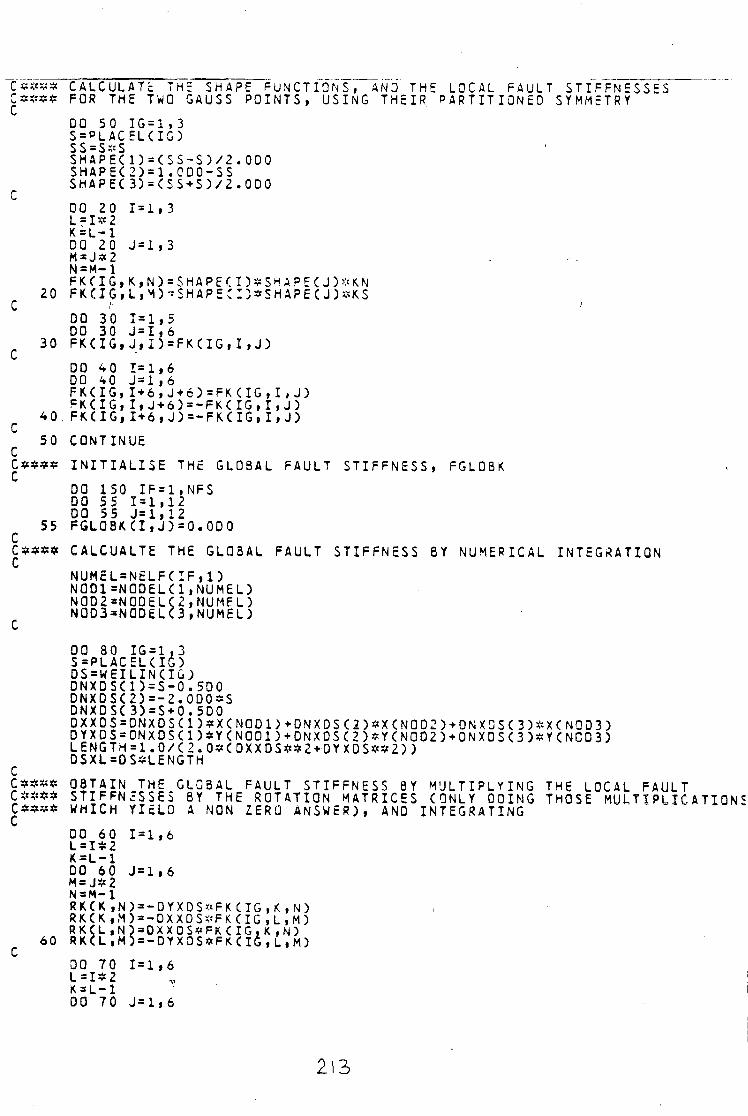
CALCULATE THE SHAPE FUNCTIONS, AN0 THE LOCAL FAULT STIFFNESSES FOR THE TWO GAUSS P O I N T S , USING T H E I R P A R T I T I O N E D SYMMETRY DO 5 0 I G = 1 , 3 S = P L A C E L C I G ) s s = s * s SHAPEC n = C S S - S ) / 2 SHAPEC 2 ) = 1.ODO-SS SHAPEC 3 ) = C S S > S ) / 2 .
1 = 1,3
0 0 0 0 0 0
20
3 0
0 0 2 0 L = I * 2 K = L - 1 DO 2 0 J = l , 3 M = J *2 N=M- 1 FKfIG»K,N)sSHAPECI)#SMAPECJ)ftKN FK(IG,L,^)"SHAPE CI5*SHAPECJ)*KS 00 3 0 1 = 1 , 5 DO 30 J = I , 6 F K C I G , J , I 3 = F K C I G , I , J ) DO 4 0 1 = 1 , 6 DO 40 J = l , 6 F K C I G , I + 6 , J + 6 ) = F K C I G , I , J ) F K C I G , I , J + 6 ) = - F K C I G , I , J ) F R C I G i I + 6 F J ) = - F K C I G i I i J ) CONTINUE INITIALISE THE GLOBAL FAULT S T I F F N E S S , FGLOBK DQ 1 5 0 I F = 1 , N F S DO 5 5 1 = 1 , 1 2 DO 55 J = l , 1 2 FGL08KCI,J)=0.0D0 CALCUALTE THE GLOBAL FAULT S T I F F N E S S BY NUMERICAL I N T E G R A T I O N N U M E L = N £ L F ( I F , 1 ) NQ01=N0DELC1» NUMEL) N0D2=N00ELC2,NUMEL) NQD3=N0DELC3,NUMEL)
G DO 80 I G = 1 , 3 S = P L A C E L C I G ) D S = W E I L I N C I G ) O N X D S U ) = S-0.5D0 D N X D S C 2 ) = - 2 . 0 D 0 * S DNXDSC 3 ) = S + 0 . 5 D 0 D X X D S = 0 N X D S C 1 ) * X C N 0 D 1 ) + 0 N X D S ( 2 ) * X C N 0 D 2 ) + 0 N X 0 S C 3 ) * X ( N Q D 3 ) D Y X D S = 0 N X D S C 1 ) * Y C N 0 0 1 ) + D N X 0 S ( 2 ) * Y C N 0 0 2 ) + D N X D S C 3 ) * Y C N C D 3 ) LENGTH=1.0/C2.0#COXXDS*3 2 + O Y X O S * # 2 ) ) DSXl=DS*LENGTH
C C***$ O B T A I N THE GLOBAL FAULT S T I F F N E S S BY M U L T I P L Y I N G THE LOCAL FAULT C**S* STIFFNESSES BY THE ROTATION MATRICES (ONLY DOING THOSE M U L T I P L I C A T I O N S C**** WHICH Y I E L D A NON ZERO ANSWER), AND I N T E G R A T I N G
DO 6 0 1 = 1 , 6 L = I * 2 K = L-1 DO 6 0 J = l , 6 M = J # 2 N = M-1 RKCK|N)a-DYXDS#FKCIG,K,N) RKCK,M)=-DXXDS*FKCIG,L,M) RK<L,N)=DXXOS*FKCIG,K,N)
60 RKCL,M)=-OYXOS#FKCIG,L,M) DO 7 0 1 = 1 , 6 L = I * 2 K = L - 1 DO 7 0 J = l , 6
213
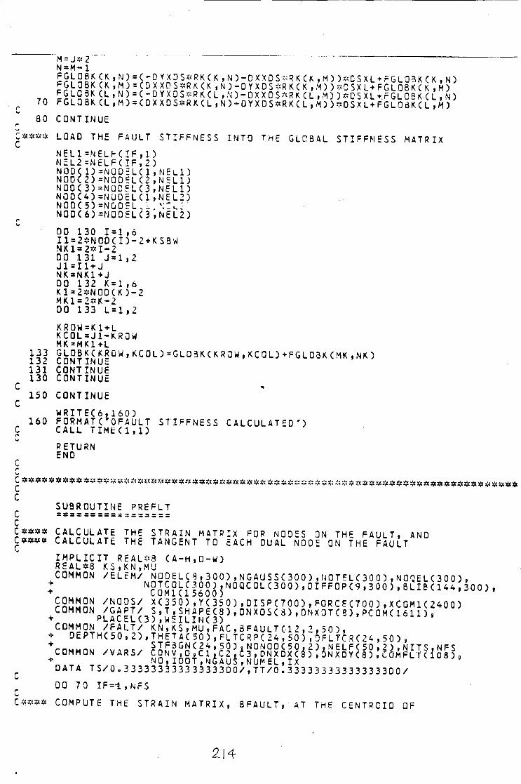
N = M- 1 = 9!-2? K^» N : ) = ( : " D Y X D S : ! ; R K C K ' N ) - D X X D S - ' ; ! ? K ^ ' H ) ) ^ C S X L ^ F G L a 3 K O < , N ) FGLQBK(K,M)=CDXXDS*RK(K,N)-0YXDS*RKCK,M))*0SXL+FGLOBKCK,M) FGLOBKCL,N) = C-DYXDS*RKCL,ND-OXXDS*RRCL,M))*OSXLtFGLOEK.CL,N)
70 FGLQBKCL,M)=CDXXOS*RKCL,N)-DYXDS*RKCL,M))#OSXL+FGLOaKCL,M) 80 CONTINUE
C « # « 4 LOAD THE FAULT S T I F F N E S S INTO THE GLOBAL S T I F F N E S S MATRIX NELl=NELf-(IF,l) NEL2 =N E L F ( I F , 2 ) NODC 1 ) = N Q D E L C 1 i N E L 1 ) N O D C 2 ) = N O D 5 L ( 2 , N 5 L l ) N 0 0 ( 3 ) = N 0 D E L ( 3 , N E L 1 ) N O D C O = N U D E L ( 1 , N E L 2 ) N O D C 5 ) = N G D E L ^ . N : U : N 0 D < 6 ) = N 0 D E L C 3 , N E L 2 ) 0 0 1 3 0 1=1,6 I l = 2 * N 0 D < I ) - 2 + K S B W N K l = 2 * I - 2 0 0 1 3 1 J * l ,2 J 1 = 1 1 + J N K = N K 1 + J 0 0 1 3 2 K = l , 6 K 1 = 2 * N 0 D ( K ) - 2 MKl=2*K-2 DO 1 3 3 L = l , 2 KROW=K1+L KC0L=J1-KRQW MK=MK1+L
H I GLOBKCKRQW,KC0L)=GL0 3K(KROW,KCOL)+FGLOBKCMK ,NK) 1 3 1 CONTINUE 1 3 0 CONTINUE
C 1 5 0 CONTINUE
C WRITE(6,160)
1 6 0 FORMAT( 'OFAULT S T I F F N E S S CALCULATED') C CALL T I M £ C 1 , 1 )
RETURN END
r-i» r <,
C SUBROUTINE PREFLT
C**3* CALCULATE THE S T R A I N MATRIX FOR NODES ON T H P FAULT, AND C«*v* CALCULATE THE TANGENT TO EACH DUAL NOOE ON THE FAULT
I M P L I C I T REAL*8 CA-H.O-W) REAL*8 K S I K N I M U COMMON /EL EM/ NODEL C <3» 3 00 ) , N GAU S S ( 300 ) , NOTEL C 30 0 ) , NOQE L C 3 00 ) ,
t N ° T C Q L C 3 0 0 ) , N O Q C O L C 3 0 0 ) , D I F F O P C 9 , 3 0 0 ) , B L I B C 1 4 4 , 300) , <NQDS/ XC 3 505 ,Y( 35 0 ) , D I S P < 7 0 0 ) , F O R C E C 7 0 0 ) , X C O M 1 C 2 4 0 0 )
COMMON 0 (/GAPT/ S , T , SH A P E C 8 ) , ONX 0 S C 3 ) , ONX0T C 8 ) , PC 0M< 1 6 1 1 ) , K « - A U t L v. 3 3 » W £ I L I N C 3 )
COMMON /FA L T / KN,KSfMU,FAC,BFAULT CI 2 , 2 , 5 0 ) , • DEPTHC50,2),THETAC 50 ) , FL TC R P C 24 , 50 ) , DF L TC R ( 24 , 50 ) , + , n M M n w y u , o e , ^ I ^ ^ G W < 2 ^ ' ^ 9 : > ^ N O y Q D S 5 9 i 2 5 2 N 6 L - F ( 5 0 , 2 ) , N I T S . N F S COMMON /VARS/ C0NV.0,C1.C2.13,DNX OXC8),ON XDYC8),COMFLTCI 08) , • NO,IOOT,NGAUS»NUMEL,IX DATA TS/0.333333333333333D0/,TT/0o333333333333333D0/ DO 70 IF = 1 , N F S
G C4#«* COMPUTE THE S T R A I N MATRIX, BFAULT, AT THE CENTROID OF
214
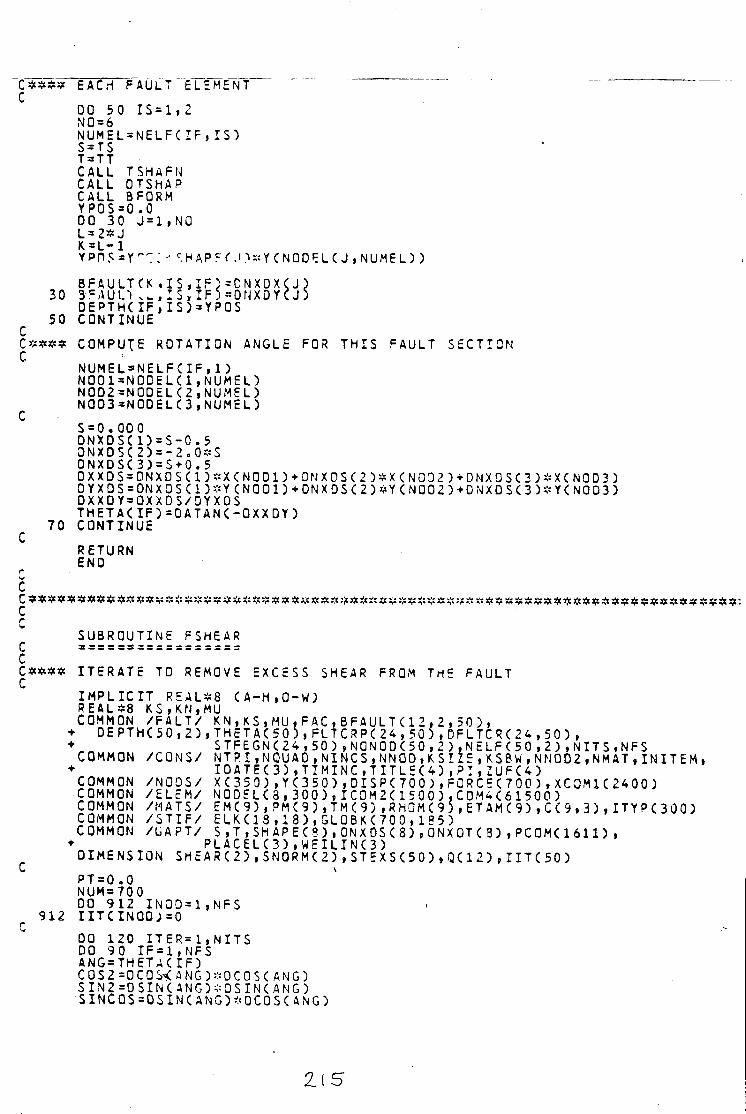
C**$* EACH FAULT ELEMENT " " C 00 50 IS=1,2 N0 = 6
NUMEL=NELF(IF,IS) S = TS T = TT CALL TSHAFN CALL OTShAP CALL B FORM YPOS=0.0 DO 30 J=1,NQ L = 2*J K=L-1 YPn5»Y'":;^HAP?<','.^YCNQDELCJiNUMEL)) BFAULTCIC,IS,IF)=CNXDXCJ)
30 3FAU1.1 .- f:S»IF5=DNXOYU5 DEPTH(IF,IS)»YPOS 50 CONTINUE C C***« COMPUTE ROTATION ANGLE FOR THIS FAULT SECTION NUMEL=NELFCIF,1) N0D1=N0DELU,NUMEL) N0D2=N0DEL(2,NUMEL) NOD3=NODEL(3 iNUME L)
C S=0.000 DNXDSCl)=S-0.5 ONXDSC 2) = -2.0*S 0NXDSC3)=S+0.5 DXXDSaDNXDSCl)*XCN0Dl)+DNXDSC2)*X<N00 2)+0NX0SC3)*XCNQD3) DYXDS = DNXDS<:i)*Y (N001)+DNXDS< 2)*Y(N002)+DNXDS<3)*Y(N003) DXXDY=OXXDS/OYXOS THETA<IF)=OATAN(-OXXDY) 70 CONTINUE C RETURN END
r
c r
SUBROUTINE F SHE A R C ================= c
ITERATE TO REMOVE EXCESS SHEAR FROM THE FAULT IMPLICIT R E A L*8 (A-H.O-W) REAL*8 KSiKNfMU COMMON /FALT/ KN,KS,MUfFAC,BFAULTC12,2 , 50 ) , + DEPTH(50,2),THETA(50),FLTCRP<24,505,DFLTCR(2^,50),
• STFEGN<24 I50),NONOOC50,2),NELF(50,2),NITS.NFS COMMON /CONS/ NTPI,MQUAD,NINCS,NN0D,KSIZE,KSBW,NN002,NMAT,INITEM, • I0ATE(3),TIMINC,TITLS<4),P!,ZUF(4) COMMON /NODS/ X ( 3 5 0 ) , Y C 3 5 0 ) , DI S P ( 70 0 ) , FO R C E ( 7 00 ) , XC OM1 C 24 00 ) COMMON /ELEM/ N0DELC 3 , 3 0 0 ) , I COM2( 1 500 ),C0M4C61500) COMMON /MATS/ EMC9),PM(9),TM(9),RHOM(95 tETAMC9)•C(9,3),ITYP(300) COMMON /STIF/ ELK(18 ,18 ) ,GL0BK<700 , 185 ) COMMON /GAPT/ S , T , SHAPEC3) , ONX OSC8),ONXOT<3),PC0M<1611) ,
• PLACELC3),WEILINC3) DIMENSION SHEARC2),SNORMC2),STEXS(50),QC12) I )IITC50) C \ PT = 0 .0 NUM=700 DO 912 IN00=1,NFS 912 IITCINOD)=0
r. DO 120 ITER=1,NITS DO 90 IF=1,NFS ANG=THETACIF) CQS2=DC0S< ANG)*DCQS( ANG) $IN2=DSIN(ANG)*0SIN(ANG) SINCOS=OSlNCANG)-.:QCOSCANG)
ZiS
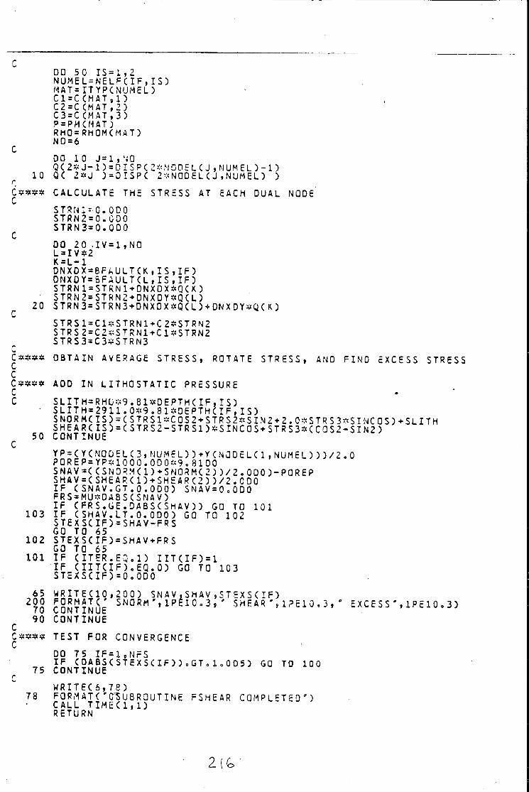
c
DO 50 IS=1,2 NUMEL=NELF(IF,IS) MAT* ITYPCNUMEL) C1 = C CHAT,1) C2=C CM AT,2 ) C3 = C CMAT,3) P=PM(MAT) RHO=RHOM(MAT) N0=6 00 10 J=1,N0 QC2*J-1) = 0ISPC2-:=M0DELC J ,NUMEL)-1) 10 QC 2*J )=DISPC 2 * N OD E L ( J »N U M E L ) )
Cs*#* CALCULATE THE STRESS AT EACH DUAL NODE STRNl'-G.ODO STRN2=0.GDO STRN3=0.ODO C 00 20 .IV = 1 ,N0 L=IV*2 K»L-1 DNXDX=BFAULTCK,IS,IF) DNXDY=BFAULTCL,IS,IF) STRN1=STRN1+DNXDX*QCK) STRN2=STRN2+0NX0Y*Q(L)
20 STRN3=STRN3+DNX0X#Q(L)+DNXDY#QCK) STRS1=C1*STRN1+C2SSTRN2 STRS2=C2*STRN1+C1*STRN2 STRS3=C3*STRN3 r
C»#*« OBTAIN AVERAGE STRESS» ROTATE STRESS, AND FIND EXCESS STRESS C C**s* AOD IN LIT HO STATIC PRESSURE C SLITH*RHU*9.81*DEPTH(IF,IS)
• SLITH*29ll.0*9.81*0EPTHCIF,IS) SNORMCIS)s(STRSl*COS2+STRS2*SIN2+2.0*STRS3*SINCOS)+SLITH SHEARCIS)=CSTRS2-STRS1)*SINC0S+STRS3*CC0S2-SIN2) 50 CONTINUE C YP=CYCNODEL(3,NUM5L))+YCN00ELCl,NUMEL)))/2.0 POREP=YP*10 00.000*9.81 DO SNAV=CCSN0RMCl)+SN0RM(2))/2.0O0)-P0REP SHAV=CSHEARC1)+SHEARC2))/2.CD0 IF CSNAV.GT.O.ODO) SNAV=0.000 FRS=MU*DABSCSNAV) IF CFRS.GE.DABSCSHAV)) GO TO 101
103 I F CSHAV.LT.0.ODO) GO TO 102 STEXSCIF)=SHAV-FRS GO TO 65
102 STEXSCIF)=SHAV+FRS GO TO 65
101 I F CITER.EQ.l) I I T C I F ) = 1 IF (IITCIF).EQ.O) GO TO 103 STEXSCIF)=0.0D0
65 WRITEC10,200) SNA V , SHAV,STEXSCIF) 2§2 SNORrt',lP6l0.3, ' SHEAR ' , 1 ? E 1 0 . 3 , EXCE SS',1PE 1 0 . 3 ) 70C0NTINUE 90 CONTINUE C
C«*** TEST FOR CONVERGENCE C
r
DO 75 IF=1 SNFS IF CDABSCSTcXSCIF))oGT olo0D5) GO TO 100 75 CONTINUE WRITEC 6,78)
78 FORMATC ' C'S U B R OUT I N E FSHEAR COMPLETED") CALL TIMEC1.1) RETURN
l\<o
c CALCUALTE THE GLOBAL FORCE COMPONENTS, BY NUMERICAL INTEGRATION 100 DO 110 IF=1,NFS NEL1=NELFCIF,1) NEL2=NELFCIF,2) N0D1=N0DELC1,NE L1) N0D2 =NODcL(2,NEL1 ) NQD3=N0DELC3,NEL1) N0D4=N00ELC1, NEL2) N0D5=N00ELC2,NEL2) N006=N0DcLC3,NEL2)
C DO 80 IG=J - 3 S=PLACELC1JJ SS=S*S 0-r-'.'FT' rr" SHAPECl)=CSS-S)/2.0 SHAPEC2)=1.0-SS SHAPEC3)=CSS+S)/2.0 DNXDSCl)=S-0.5 ONXOSC2)=-2.0*S ONXDSC3)=S+0.5
C DXXDS=DNXDSC1)*XCNQ01)+DNXDSC2)#XCNQD2)+0NXDSC3)*XCN003) DYXDS=ONXDSCl)sYCN001)+DNXDSC2)*YCN002)+DNXOSC3)*YCN0 03) TAU=CSHAPEC1)*STEXSCIF)+SHAPEC2)*STEXSCIF)+ + SHAPEC3)*STEXS(IF))*FAC $1DST=SHAPEC1)*DS*TAU S2DST=SHAPEC2)*CS*TAU S3DST=SHAP5C3)*OS*TAU FORCEC 2*N0D1-1)=F0RCEC2*N0D1-1) + C S10STSDXXDS) FORCEC 2*NDD1 )=FORCEC 2*N0D1 )+CSlDST$DYXDS) F0RCEC2*N002-1)=FORCEC2*NOD2-l)-KS2DST*DXXDS) FORCEC 2SN3D2 )=FORCEC 2*NOD2 ) + CS2DST*0YXDS) FORCEC2*NOD3-l)=FORCEC 2*N0D3-1) + CS3DST*DXX0S ) FORCEC 2*N0D3 )=FORCEC 2*N0D3 )+CS3DSTSDYXOS) F0RCEC2*N0D4-l)=FaRCEC2*N0D4-l)-CSlDST«0yXDS) FORCEC 2*N0D4 )=FQRCEC 2*N0D4 )-CS 1 DST*0YX0S) FORCEC 2*NCD5-1)=FORCEC 2*N0D5-1)-CS2DST*DXXDS) FORCEC 2*N0D5 )=FORCEC 2*NOD5 )-CS2DST*DYXDS) F0RCEC2*N0D6-1)=F0RCEC2*N0D6-1)-CS3DST*QXX0S)
80 FORCEC 2*N006 )=FORCEC 2#N006 )-CS3DST*0YXDS) 110 CONTINUE
C C**** RESOLVE STIFFNESS EQUATION
00 115 IC0P=1,NNG02 115 OISPCICOP)=FORCECICOP)
CALL MA07BDCGL03K, 01SP,NUM,NNQD2,KSIZE,PT) WRITEC6,620)ITER
620 FQRMATC " ENO OF ITERATION 14) 120 CONTINUE
C WRITEC6,140)
140 FORMATC'C**** EXECUTION STOPPED IN FSHEAR : • 'EXCESS SHEAR STRESS HAS NOT CONVERGED') CALL TIMEC1,1) STOP END
C C C ********* **********«***:**#fc$**#S^ c C
SUBROUTINE SURF C = = 3 S = 3 S = = = = = = = =
c C**** PLOT THE DISPLACEMENT PROFILE 3 F SPECIFIED NODES
IMPLICIT? REAL*8 CA-H.O-W) COMMON /NUDS/ XC350),YC350),DISPC700),FORCE(700),XCOM1C2400) OIMcNSION NNC2),XPC2,50),YOISPC2,50),XPLTC50),YPLTC50)
217
XSTART=1„0E50 XENO=0.0 YBOT=0.0 YTQP=0.0 READ<4,1G)N0SECT 10 FORMAT(Ib) DO 20 IS=1,N0SECT READ (4 ,10)NN<IS) N0=NN(IS) DO 20 IN=1,N0 READ(4,1G)N00 XPCIS,IN)=X(NCD) YDISP<IS,IN)=DISPC2*NQD) YD=YOISPCIS,IN) XD=XPCIS,IN) XSTART=AMIN1CXSTART,XD) XF.N0=AMAX1(XEND , XO) YB0T-AMAX1CYB0T,YD) 20 YT0P=AMIN1(YT0P,YD)
r XSTART=XSTART/1000.0 XEND=*5ND/1000. 0 CALL CSPACEC0.0,1.2,0.0,1.0) CALL PSPACE(0.1,1.1,0.25,0.5) CALL MAP<XSTART,XEN0,YT0P,YB0T) CALL AXES
C DO 30 IS=1,N0SECT NQ=NN(IS) DO 40 IN=1,N0 XPLTCIN)=XPCIS,IN)/1.0E3 40 YPLT<IN)=YDISP(IS,IN) 30 CALL CURVEOCXPLT,YPLTS1,N0) RETURN ENO
C c c c SUBROUTINE FAIL r — — — — — _ _ _ — — — — c CSSS* CALCULATES WHETHER FAILURE HAS OCCURED AT EACH STRESS C***3 GAUSS POINT IN EACH ELEMENT C IMPLICIT PFALS8 (A-H.O-W)
COMMON /CONS/ NTRI,NQUA0,NINCS,NN00,KSI2E, KSBW,NNQD2,NMA T,INITEM, + IDATE(3),STMAX,TITLE(4),PI,IUF<4) COMMON /NODS/ X(350) , Y(350 ),DISP(700),F0RCEC700),XSTPOSC4, 300), • YSTPOSC4,300) COMMON /EL EM/ N0DELC8.300),NGAUSSC300),NOTEL(300),NOQEL(300), • NOTCOLC300),NOQCOLC300),DIFFOP(9,300),aLIBC144,300), • PRINCC16 ,300),CREEP(36 , 300 ) COMMON /FALE/ STRO<4,350),CFAIL(4,?00),FANGLC4,300),IFAIL(4,300) COMMON /MATS/ EMC9),PM<9),TM(9),RHOMC9),ETAMC9),CC9,3),ITYPC300) FMU*1.0 PHI=OATANC1.0/FMU)*9 0.Q/PI NOEL=NTRI NO = 3
C CxtZV* START LOUP OVER TRIANGULAR AND QUADRILATERAL ELEMENTS
DO 700 IT = 1 , 2 IF CIT.EQ.l) GO TO 20 NQEL=NQUAO N 0 » 4
20 IF CNOEL.EQoO) GO TO 700 DO 550 IEL=l,NOEL IF (IT.Ew7l)HUMEL=NOTELCIEL) IF (IT.EQ.2)NUMEL=NOQELCIEL)
MAT=ITYP(NUMEL) ' " T=TMCMAT) SC=-4.19*T DO 555 IG=l,NO JPOS=C IG-1 )*4
C#*«* ADD LITHGSTATIC PRESSURE TO EACH 0F THE PRINCIPAL STRESSES DEPTH = YSTPOS( IG ,NUMEL) HY0=RH0M(ITYPCNUMEL))*9.S1*0EPTH Pl=PRINC(l+JPOS,NUMEL)+HYD P2=PRINCC2+JP0S,NUMEL)+HY0 S1=0MAX1(P1,P2) S3=0MIN1CP1,P2) SM=<Sl+S3)/2.0 TB=CSl-S3)/2 .0
C**3* TENSIONAL REGION C IF CS'M.LT.T) GO TO 551 IFAILCIG,NUMEL)=-1 CFAILCIG,NUMEL)=(T-SM)/T FANGLCIG,NUMEL)=0.0 GO TO 555
551 I F (SM.LT.-T)GO TO 552 IFAILCIG,NUMEL)=1 CFAILCIG,NUMEL)=CT-S1)/CT-SM) FANGLCIG,NUMEL)=0.0 GO TO 555
C C**#* OPEN CRACK. C OM P R E S SI ON A L REGION
552 SA = SC-2.C=.-T IFCSM.LT.SA) GO TO 553 IFAILCIG,NUMEL)=2 TF=0SQRTC-4.0*T*SM) CFAILCIG,NUMEL)=1.0-TB/TF FANGLCIG,NUMEL)=OARCOSC-TF/SM/2.0)*90.0/PI GO TO 555 C
0**3* INTERMEDIATE REGION 55 3 BETA=2.0/FMU#OSQRT(1.0-SC/T)+SC/T
S3 = SC*!C1.0 + FMUsFMU) + BETA*FMU*FMUST TC=3ETA*FMU*T-FMU*SC I F CSM.LT.SB) GO TO 554 IFAILCIG,NUMEL)=3 CFAILCIG,NUMEL)=1.0-T3/DSQRTCCSM-SC)*CSM-SC)+TC*TC) FANGLCIG,NUMEL)=DATANCTC/CSC-SM))*90.0/PI GO TO 555
C C**#* CLOSED CRACK. C 0 MP R E S SI 0 N AL REGION
554 ALPHA=OS^RTClo 0+FMU*FMU)/FMU IFAILCIG,NUMSL)=4 CFAILCIG,NUMEL)=1.0-ALPHASTB/C3ETA*T-SM) FANGLfir, .NI1M = I i : P H T
C
C
FANGLCIG,NUMEL)=PHI 555 CONTINUE 550 CONTINUE 700 CONTINUE WRITEC6,10) 10 FORMATC'OFAILURE CRITERIA CALCULATED') CALL TIMEC1,1) C
600 RETURN END r w C C 5*^^^^ C C
z n
SUBROUTINE OISVEC C ================= c C*ZX* PLOTS THE DISPLACEMENT VECTOR AT EACH NODE
IMPLICIT REAL-8 (A-H,0-W) REALMS KN,KS,MU COMMON /NODS/ XC350),Y(350),DISPC700),FORCEC700),XCOM1(2400) COMMON /FALT/ KN,KS,MU,FAC,BFAULTC12,2,50),
+ OEPTH(50,2),THETAC50),FLTCRP(24,50),OFLTCRC24,50), • STFSGNC24.50),NONODC50,2),NELF(50,2),NITS,NFS COMMON /CONS/ NTRI , NQUAD,NINCS,NN00,KSIZE,KSBW,NNOD2,NMAT,INIT£M, • IDATEC3),STMAX,TITLE(4),PI,ZUF(4) COMMON /VARS/ XMAX,XMIN,YMAX,YMIN,XOMAX,XOMIN,YQMAX,YOMIN,
X £ P , Y S P v Y. V EC S , v V E C S , P LT 0 ( 1 2 3 ) , NC , N'J ME !_ , ~u 3 , L COM : 2 ) COMMON /ELEM/ NODEL( 8 , 300 ),NGAUSS( 300),NOT ELC300) tNOQELC300) f + N OTCCLC300),NOQCOLC 300), OIFFOPC 9, 30H'i.ftL 13(144, 300), + F'RINC(16 ,300),CREEP(36 ,300) DIMENSION XPLTC3) , YPLTC3) C C**$* FIND THE LARGEST DISPLACEMENT, DIMAX DIMAX=0,ODD DO 10 I=1,NN0D DVEC*0SQRT(DISPCI3 2-1)**2+0ISP(I#2>**2)
10 DIMAX=DMAX1CDVEC,DIMAX) 0*3$* SET UP PLOT COORDINATES
XSPl=XSP+0.2 CALL CSPACEC0.2,'XSP1,0.0,1.0) CALL PSPACECO.2,XSP1 ,0.0,1.0) CALL MAPCXMIN,XMAX , YOMIN,YOMAX)
C**** PLOT A CIRCLE AT EACH NODE C
CALL CTRSETC4) CALL CTRMAGC7) CALL PTPL0T(X,Y,1 ,NN0D,54) CALL CTRMAGC15) CALL CTRSET(l)
C***S PLOT DISPLACEMENT VECTOR XVECS=ABS(XMAX-XMIN)/(25.0*XSP) YVECS=ABS(YMAX-YMIN)/C25.0*YSP) SCALEX=XVECS/DIMAX SCAL EY = YVECS/DIMAX DO 20 I=1,NN0D CALL POSITN(XCI),YCI ) ) XPL=X(I)-KDISP(I*2-1)*SCALEX) YPL=Y(I)-KDISPCI*2)*SCALEY) 20 CALL JOINCXPL,YPL)
C**$* PLOT POSITION OF FAULT, IF ONE IS PRESENT IF CNFSoEQ.O) GO TO 60 DO 70 IF=1,NFS NUMEL SNELF(IF,1) N0D1=N0DELC1.NUMEL) N0D2=NCDEL(2»NUMEL) N0D3=N0DEL(3,NUMEL) XPLTC1)=X(N0D1) YPLTCl)=Y(N0D1) XPLT(2)=XCN0D2) YPLT(2)=Y(N0D2) XPLTC3)=X(N0D3) YPLTC3)=YCN0D3) 70 CALL CURVE0CXPLT 9YPLT,l f3)
Csxs#* ANNOTATE THE PLOT C ?
60 XSPl=XSP+0.4 CALL PSP«CE(0.0,XSP1,0.0,1.0)
2zo
CALL CSPACECO.O,XSP1,0.0,1.0) CALL MAPCXOMIN.XOM AX,YOMIN,Y O.MAX) XMAP1=(XMAX-XMIN)/XSP XCEN=CXMAX+XMIN)$0.5 XLABEL = XCEN-CC13.0/7'7.0)*XMAP1) YLAEEL=CYMAX-YMIN)*0.15 CALL P0SITMCXLA3EL,YLA3EL) XLABEL=XLA3EL+100.0*SCALEX CALL J0INCXLA8EL,YLABEL) CALL PLOTCSCXLABEL,YLABEL,' 100 METRES',12) X S T = XC EN- C C 7 . 0 / 7 7 . 0 ) * XM A P 1 ) YST=(YMAX-YMIN)*0.32 CALL PLOTCSCXST,YST, 'DISPLACEMENT VECTORS',20) ADD TITLE AND LABEL AXES CALL LABEL
11
C C C c c c c # # # * c * # * # c
WRITEC6.il) FORMAT C'00 ISPLACEMENTS RETURN END
PLOTTED ')
SUBROUTINE TANOM
INCORPORATE INIT I A L STRAINS DUE TO TEMPERATURE ANNOMALIES INTO THE FORCE VECTOR IMPLICIT REAL R E A L * 8 K N , K. S , COMMON /CONS/ COMMON /EL EM/
*8 CA-H.Q-W) MU
• +
+
U !l JI"i N9UAD,NINCS,NNOO,KSIZE,KSPW,NNaD2,NMAT,INITEM f IDATEC3),TIMINC,TITLEC4),PI,ZUFC4) NODELC8,300),NGAUSSC300),NOTELC300),NOQELC300), NpTCOLC300),NOQCOLC300),DIFFOPC9,300),BLIBC144,300), COM1C15600) EMC9),PMC9),TMC9),RH0MC9),ETAMC9),CC9,3),ITYPC300) S,T,SHAPEC3),DNXDSC3),0NXDTC8),TSHAPEC6,36), TDNXDSC6,36),TDNX0TC6,36),TW1W2C6,6),QSHAPEC3,72), 9DNXDSC3,72),QDNXDTC3,72),QW1W2C3,9),C0M2C258)
XC350),YC350),DISPC70 0),FORCEC700),XCOM1C2400)
D I M E N S I O N A N 5 D C 8 ) R 0 C 4 ' 3 5 0 ) , c f a i l ( 4 ' 3 0 ^
COMMON /MATS/ COMMON /GAPT/
COMMON /NODS/
NODES WITH TEMP ANOM C*$** IN I T I A L I S E , THEN READ IN NO. C INITEM=1 DO 10 1=1,4 DO 10 J=l,NNOD
10 STROCI,J)=0.0D0 REAOC3,20)NNODT
20 F0RMATCI5,F10.3) c Cs*s* READ IN THE TEMP ANOMALY OF EACH NODE, AND CALCULATE THE r""*~~ I N I T I A L STRAIN COMPONENTS C
DO 30 I=l,NNODT READC3 ,20)NODT,DELT ALPH=1.OE-5 STROCI ,NODT)=-l.2 5*ALPH*DELT STR0C2 ,NODT)=STROC1,NODT) 30 CONTINUE C
C*$*s CALCUALTE THE FORCE VECTOR FOR EACH NOEL^NTRI N0 = 6 DO 90 IT=1,2 IF CIT.EQ.4) GO TO 200 NOEL =NQUAD' NO = 8
ELEMENT
211
2 0 0 I F (NOEL.EQ.0) GO TO 90 ' ~ C DO 8 0 I E L = l » N O F L I F ( I T . E C . 2 ) GQ TO 800 N U M E L = N O T E L ( I E L ) NROW=NOTCOL(IEL) GO TO 9 0 0
80 0 N U M E L = N O Q E L ( I E L ) NROW=NOQCOLCIEL)
900 CONTINUE I U S E = 0 DO 4 0 1=1,MO N O D C I ) = N O D E L ( I , N U M F L ) I F CIUSE.EQ.0.AND.STR0C1, N 0 0 ( I ) ) . N E . 0 . 0 ) I U S E = 1
40 CONTINUE C IF CIUSE.EQ.O) GO TO 80
C N G A U S = N G A U o o v. N U M E L ) MAT=ITYPCNUMEL) C l = C ( M A T , l ) C2=CCMAT,2) C 3 = C ( M A T , 3 ) DO 7 0 IG=1,NGAUS DV=OIFFOPCIG,NUMEL) I P O S = < I G - l ) * N 0 J P 0 S = I P 0 S * 2 ST0X=O.0D0 STOY=0.0D0 S T 0 X Y = 0 . 0 D 0
C C**** CALCUALTE I N I T I A L S T R A I N AT T H I S GAUSS POINT
I F C I T . E Q . 2 ) GO TO 1 0 0 DO 5 0 I V = l , N O S H A P =TSHAPE(NROW,IPOS+IV) STOX=ST0X+SHAP*STROClINODCIV)) S T 0 Y = S T 0 Y + S H A P * S T R 0 C 2 , N O D ( I V ) )
5 0 ST0XY=STOXY-t-SHAP*STRO(3,NODCIV)) GO TO 1 1 0
10 0 0 0 1 2 0 I V = 1 , N 0 SHAP=QSHAPECNR0W,IP0S+IV) STOX=STOX+SHAP*STRO(1,NODCIV)) S T 0 Y = S T 0 Y + S H A P * S T R O C 2 , N O D C I V ) )
120 S T 0 X Y = S T 0 X Y + S H A P * S T R 0 C 3 , N O D ( I V ) ) 1 1 0 CONTINUE C
C**** O B T A I N THE I N I T I A L S T R A I N FORCE VECTOR 3Y NUMERICAL INTEGRATION P=PMCMAT) S T 0 Z = S T 0 X / ( 1 . 0 * P ) STOX =ST0X + P*ST0Z S T 0 Y = S T 0 Y + P * S T 0 Z 0 0 6 0 1=1,NO L = 2 * I K = L - 1 D N D X = 3 L I 5 C J P 0 S + K , N U M S L ) DNDY=BLIb(JPOS+L,NUMEL) FQRCEC2*NODCI)-1)=FORCEC2*NOOCI)-1)+CCDNOX*C1*STOX
* +ONOX*C2*ST0Y+ONOY*C3*ST0XY)*OV) FORCEC 2 * N 0 D ( I ) ) = F O R C E ( 2 * N 0 D < I ) ) + (CQNDY*C2*ST0X
• +DNDY*C1*ST0Y+DNDX*C3*ST0XY)*DV) 60 CONTINUE 70 CONTINUE 80 CONTINUE 90 CONTINUE
C WRITEC6.160)
160 FORMATC 'OSTRAIMS DUE TO TEMPERATURE ANOMALY CALCULATED * ) CALL T I M E <1 , 1 ) RETURN END
C
111
NGTCOLC300),NOqCOL(300),DI PRINCC16 ,300),CREEP(36, 300)
C SUBROUTINE DEVST C ================ C C C A L C U L A T h S THE DEVIATORIC STRESS VECTORS C*$s* AND STORdS THEM IN PRINC C IMPLICIT
COMMON /CONS/ + COMMON
+ SIMAX=0.0 NSGAUS=3 NF.L = NTRI DO 50 IS=1,2 IF (IS.Eg.1) GO TO 10 NSGAUS=4 NEL=NQUAU 10 CONTINUE DO 40 IEL = 1» NEL IF ( I S . E C i . l ) NUMEL = NOTEL(I EL) IF (IS.EQ.2) NUMEL=NOQEL(IEL) DO 30 IG=1,NSGAUS JPOS=CIG-l)*4 HYD=(PRINC(JP0S+1,NUMEL)+PRINC(JP0S+2,NUMEL)+ + PRINC(JPOS+3,NUMEL))/3.0 DO 20 1=1,3
20 PRINC(JPGS+I,NUMEL)=PRINC(JPOS+I,NUMEL)-HYD PRINC(JPGS+I,NUMEL)=PRINC(JPOS+I, NUMED-H YD STMAX=DMAX1(DABS(PRIMCd*JPOS,NUMEL)),DA6S(PRINC(2+JP0S,NUMEL)), 1 DAbS(PRINC(3+JPOS,NUMEL)),STMAX) 30 CONTINU-40 CONTINUE 50 CONTINUE RETURN END
2 Z S
REFERENCES
Andrews, D.J. and S l e e p , M.H., 197 4. Nuir.eri.cal m o d e l l i n g o f t e c t o n i c f l o w
b e h i n d i s l a n d a r c s . G eophys. J • R. a s t r . Soc . , 38, 2 3 7 - 2 5 1 .
A r t y u s h k o v , E.V., 1973. S t r e s s e s i n t h e l i t h o s o h e r e c a u s e d by c r u s t a i
t h i c K n e s s i n h u i n o g e n e i t i e s . J_;_ Ceophyz . Res . , 73, 7 5 7 5 - 7 7 0 3 .
Ashby, M.i. d i i ^ e r r a l l , R. A, , 1978. Micromerhan i sms of f l o w and f r a c t u r e
and t h e i r r e l e v a n c e t o t h e r h e o l o g y of t h e upper m a n t l e . Ph.il .
T r a n s • R^ Soc., 200A, 59-95.
B a r a z a n g i , M. and I s a c k s , B., 1971. L a t e r a l v a r i a t i o n s o f s e i s m i c wave
a t t e n u a t i o n i n t h e upper m a n t l e above t h e i n c l i n e d e a r t h q u a k e z one o f
t h e Tonga i s l a n d a r c s y s t e m : deep anomaly i n t h e upper m a n t l e . J .
G e ophys. R e s . , 76, 3493-3516.
B a r a z a n g i , M., P e n n i n g t o n , W. and I s a c k s , B., 197 5. G l o b a l s t u d y o f
s e i s m i c wave a t t e n u a t i o n i n t h e upper m a n t l e b e h i n d i s l a n d a r c s u s i n g
pP w a v e s . Geophys. R e s . , 30, 1079-1092.
B a r k e r , P.F. and H i l l , I.A., 1981. Back a r c e x t e n s i o n i n t h e S c o t i a S e a .
P h i l . T r a n s . R^ S o c . Lond. A, 300, 249-262.
B a r l o w , J . , 1976. O p t i m a l s t r e s s l o c a t i o n s i n f i n i t e e l e m e n t s . I n t . J .
Numer. Meth. Eng., 10, 2 4 1 - 2 5 1 .
B a r r e l , J . , 1914. The s t r e n g t h of t h e e a r t h s c r u s t . G e o l . , 22, 729.
B e n i o f f , H., 1954. O r o g e n e s i s and deep c r u s t a i s t r u c t u r e : a d d i t i o n a l
e v i d e n c e from s e i s m o l o g y . G e o l . S o c . Amer. B u l l • , 6 5 , 3 85-400.
B i b e e , L.D., S h o r , G.C., and Lu, R., 1980. I n t e r - a r c s p r e a d i n g i n t h e
M a r i a n a t r o u g h . M a r i n e G e o l . , 35, 183-197.
B o d i n e , J.H. a n c W a t t s , A.B., 1979. L i t h o s p h e r i c f l e x u r e s e a w a r d o f t h e
B o n i n and M a r i a n a t r e n c h e s . E a r t h P l a n e t . S c i . L e t t . , 43, 132-148.
B o t t , M.H.P., 1971. The i n t e r i o r o f t h e e a r t h , A r n o l d .
- 22 4 -
B o t t , M.H.P., 1982a. The i n t e r i o r o f t h e e a r t h ( 2 n d E d i t i o n ) . A r n o l d .
B o t t , M.H.P., 1982b. The mechanism of c o n t i n e n t a l s p l i t t i n g .
T e c t o n o p h y s i c s , 81, 301-309.
B o t t , M.H.P. and Dean, D.5., 1972. S t r e s s s y s t e m s a t young c o n t i n e n t a l
m a r g i n s . N a t u r e (Phy s . S c i . ) , 235, 23-25.
B o t t , M.H.P. and K u s z n i r , N.J., 1979. S t r e s s d i s t r i b u t i o n s a s s o c i a t e d
w i t h c o m p e n s a t e d p l a t e a u u p l i f t s t r u c t u r e s w i t h a p p l i c a t i o n t h e
c o n t i n e n t a l s p l i t t i n g mechanism. Geophys. J . R. a s t r . S o c . , 56,
451-459.
B r a c e , W.F., 1964. B r i t t l e f r a c t u r e o f r o c k s . I n : W.R. Ju d d ( e d i t o r ) .
S t a t e of s t r e s s i n t h e e a r t h ' s c r u s t . E l s e v i e r , New Yo r k , N.Y.,
111-174.
C a l d w e l l , J.G, Haxby, W.F., K a r i g , D.E. and T u r c o t t a , D.L., 1976. On t h e
a p p l i c a b i l i t y o f a u n i v e r s a l e l a s t i c t r e n c h p r o f i l e . E a r t h P l a n e t .
S c i . L e t t . , 31, 239-246.
C a r t e r , N.L., 1976. S t e a d y s t a t e f l e w of r c o k s . Rev. G e o p h y s . S p a c e
P h y s . , 14, 301-360.
Chapman, M.E. and T a l w a n i , M., 1982. G e o i d a n o m a l i e s o v e r deep s e a
t r e n c h e s . Geophys. R^ A s t r . S o c . , 68, 349- 3 6 9 .
C h a p p i e , W.M. and T u l l i s , T.E., 1977. E v a l u a t i o n o f t h e f o r c e s t h a t d r i v e
t h e p l a t e s . J_;_ G e ophys. R e s . , 32, 1967-1984.
C h a p p i e , W.M. and F o r s y t h , D.W.., 1979. E a r t h q u a k e s and b e n d i n g o f t h e
p l a t e a t t r e n c h e s . J_;_ G e ophys. R e s . , 34, 57 2 9 - 6 7 4 9 .
C h r i s t e n s e n , D.H. and R u f f , L . J . , 1983. O u t e r r i s e e a r t h q u a k e s and
s e i s m i c c o u p l i n g . G eophys. R e s . L e t t . , 10, 697-700.
C h a s e , C , 1978. E x t e n s i o n b e h i n d i s l a n d a r c s and m o t i o n s r e l a t i v e t o
h o t s p o t s . Geophys. R e s . , 83, 5335-5337.
Chen, A.T., F r o h l i c h , C. and Latham, G.V., 1982. S e i s m i c i t y o f t h e
f o r e a r c m a r g i n a l wedge ' a c c r e t i o n a r y p r i s m ) . Geophys . Res . , 37,
3679-3690.
Cook, R.D., 1981. C o n c e p t s and a p p l i c a t i o n s of f i n i t e e l e m e n t a n a l y s i 5
(2nd E d i t i o n ) . Wi1 ay.
D a v i e s , G.F., 1930. M e c h a n i c s of s u b d u c t e d l i t h o s p h e r e . G e o p h y s .
Res, 85, 6 3 0 4 - 6 3 1 3 .
D a v i e s , G.F., 1981. R e g i o n a l c o m p e n s a t i o n o f s u b d u c t e d l i t h o s p h e r e :
e f f e c t s on g e o i d , g r a v i t y and t o p o g r a p h y from a p r e l i m i n a r y m o d e l .
E a r t h P l a n e t . S c i . L e t t . , 54, 4 3 1-441.
D a v i e s , G.F., 1983. S u b d u c t i o n zone s t r e s s e s : c o n s t r a i n t s from m e c h a n i s m s
and from t o p o g r a p h i c and g e o i d a n o m a l i e s . T e c t o n o p h y s i c s , 99, 8 5 - 9 8 .
Dean, D.S., 1973. S t r e s s a n a l y s i s o f t h e l i t h o s p h e r e . U n p u b l i s h e d Ph.D.
t h e s i s . U n i v e r s i t y of Durham.
D e s a i , C.S. and A b e l , J . F . , 1972. I n t r o d u c t i o n to t h e f i n i t e e l e m e n t
method. Van N o s t r a n d R e i n h o l d .
D i c k e n s o n , W.R. and S e e l y , D.R., 1979. S t r u c t u r e and s t r a t i g r a p h y o f
f o r e - a r c r e g i o n s . B u l l . Am. P e t r o l . G e o l . , 63, 2-31.
E g u c h i , T., Uyeda, S. and Maki, T., 1979. S e i s m o t e c t o n i c s and t e c t o n i c
h i s t o r y i n t h e Andaman s e a . T e c t o n o p h y s i c s , 57, 3 5 -51.
E i s e n b e r g , M.A. and M a l v e r n , L . E . , 1973. On f i n i t e e l e m e n t i n t e g r a t i o n i n
n a t u r a l c o - o r d i n a t e s . I n t . J . Numer. Meth. Eng. , 7, 5 7 4 - 5 7 5 .
E l s a s s e r , W.M., 1969. C o n v e c t i o n and s t r e s s p r o p a g a t i o n i n t h e upper
m a n t l e . I n : S.K. R u n corn ( E d i t o r ) , The a p p l i c a t i o n o f modern
p h y s i c s t o t h e e a r t h and p l a n e t r y i n t e r i o r s . W i l e y . New Y o r k .
223-246 .
E l s a s s e r , W.M., 1971. S e a f l o o r s p r e a d i n g a s t h e r m a l c o n v e c t i o n . J .
Geophys . R e s . , 76, 1101-1112,
E n g d a h l , E.R. and S c h o l z , C.H., 1977. A d o u b l e B e n i o f f z o ne b e n e a t h t h e
- 226 -
A l e u t i a n s : an u n b e n d i n g o f t h e l i t h o s p h e r e . G e o p h y s . R E s . L e t t . ,
4, 473-476.
E n g l a n d , P. and W o r t e l , R., 1980. Some c o n s e q u e n c e s o f t h e s u b d u c t i o n of
young s l a b s . E a r t h P l a n e t , S c i . L e t t . , 47, 403-415.
F e l i p p a , C.A., 1966. R e f i n e d f i n i t e e l e m e n t a n a l y s i s o f l i n e a r and
n o n l i n e a r two d i m e n s i o n a l s t r u c t u r e s . U n p u b l i s h e d Ph.D. t h e s i s .
U n i v e r s i t y of C a l i f o r n i a , B e r k l e y .
F o r s y t h , D.W., 1977. The e v o l u t i o n o f t h e upper m a n t l e b e n e a t h mid o c e a n
r i d g e s . T e c t o n o p h y s i c s , 38, 39-118.
F o r s y t h , D.W. and Uyeda, S., 1975. On t h e r e l a t i v e i m p o r t a n c e o f t h e
d r i v i n g f o r c e s of p l a t e m o t i o n . Geophys J . R. a s t r . S o c . , 43,
163-200.
F u j i t a , K. and Kana m o r i , H., 1981. Double s e i s m i c z o n e s and s t r e s s e s o f
i n t e r m e d i a t e d e p t h e a r t h q u a k e s . Geophys• J . R. A s t r . S o c . , 66,
131-156 .
G o l d s m i t h , W., Sackman, J . L and E w e r t , F., 1976. S t a t i c a nd d y n a m i c
s t r e n g t h of B a r r e g r a n i t e . I n t . J . r o c k Mech. Ming. S c i . , 13,
303-309.
Goodman, R.E., T a y l o r , R.E., and B r e k k e , T.L., 1968. A model f o r t h e
m e c h a n i c s of j o i n t e d r o c k . S o i l Mech. and Found. P r o c . ASCE.,
94, 637-658.
G r e l l e t , C. and D u b o i s , J . , 1982. The d e p t h of t r e n c h e s a s f u n c t i o n o f
t h e s u b d u c t i o n r a t e and a g e of t h e l i t h o s p h e r e . T e c t o n o p h y s i c s , 82,
45-56.
G r i g g s , D.T., 1972. The s i n k i n g l i t h o s p h e r e and the f o c a l m e c h a n i s m o f
d e e p e a r t h q u a k e s . I n : E.G. R o b e r t s o n ( E d i t o r ) , M ature o f t h e s o l i d
e a r t h . M c G r a w - H i l l , New Y o r k , N.Y., 361-384.
Hanks, T.C., 1971. The K u r i l t r e n c h - H o k k a i d o r i s e s y s t e m : l a r g e s h a l l o w
- 227 -
e a r t h q u a k e s and s i m p l e models of d e f o r m a t i o n . G e o p h y s . J • R. a s t r .
S o c . , 23, 173-189.
H a r p e r , J . F . , 1975. On t h e d r i v i n g f o r c e s of p l a t e t e c t o n i c s . G e o p h y s .
LL LL a s t r . S o c . , £0, 465-474.
Hasebe, K., F u j i i , N. and Uyeda, S., 1970. T h e r m a l p r o c e s s e s u n d e r i s l a n d
a r c s . T e c t o n o p h y s i c s , 10, 335-355.
Haxby, W.F. and T u r c o t t e , D.L., 1976. S t r e s s e s i n d u c e d by t h e a d d i t i o n o r
r e m o v a l o f o v e r b u r d e n and a s s o c i a t e d t h e r m a l e f f e c t s . G e o l o g y , 4,
181-184 .
Hayes, D.E. and Ewing, M., 1970. P a c i f i c b o u n d a r y s t r u c t u r e . I n : A.E.
M a x w e l l ( e d i t o r ) , The S e a . I d e a s and o b s e r v a t i o n s on p r o g r e s s i n t h e
s t u d y of t h e s e a s . 4, 29-72. W i l e y - I n t e r s c i e n c e , !>few Y o r k . N.Y.
H s u i , A.T. and T o k s o z , M.N., 1981. Back a r c s p r e a d i n g : t r e n c h m i g r a t i o n ,
c o n t i n e n t a l p u l l o r i n d u c e d c o n v e c t i o n ?. T e c t o n o p h y s i c s , 74, 8 9 - 9 8 .
I s a c k s , B., O l i v e r , J . and S y k e s , L.R., 1968. S e i s m o l o g y and t h e new
g l o b a l t e c t o n i c s . Geophys. R e s . , 73, 5 8 5 5 - 5 8 9 9 .
I s a c k s , B. and M o l n a r , P., 1969. M a n t l e e a r t h q u a k e mechanisms and t h e
s i n k i n g o f t h e l i t h o s p h e r e . Mature, 223, 1121-1124.
I s a c k s , B. and Molnar, P., 1971. D i s t r i b u t i o n o f s t r e s s e s i n t h e
d e s c e n d i n g l i t h o s p h e r e from a g l o b a l s u r v e y o f f o c a l m e c h a n i s m
s o l u t i o n s of m a n t l e e a r t h q u a k e s . Rev• Geophys• S p a c e P h y s . , 9,
103-174
I s a c k s , B. and B a r a z a n g i , M., 1977. Geometry of B e n i o f f z o n e s : l a t e r a l
s e g m e n t a t i o n and downwards b e n d i n g o f t h e s u b d u c t e d l i t h o s p h e r e . I n :
M. T a l w a n i and W.C. P i t t m a n I I I ( E d i t o r s ) , I s l a n d a r c s , d e e p s e a
t r e n c h e s and b a c k a r c b a s i n s . M a u r i c e Ewing S e r . , Am. G e o p h y s .
U n i o n , 1, 163-174.
J a e g e r , J . C . and Cook, N.G.W., 1976. F u n d a m e n t a l s of r o c k m e c h a n i c s .
- 228 -
Second e d i t i o n , Chapman and H a l l s c i e n c e p a p e r b a c k s .
J u r d y , D.M., 1979. G l o b a l p l a t e r e o r g a n i s a t i o n s and s p r e a d i n g i n back a r c
b a s i n s . Geophys• Res, 34, 6796-6802.
Kanamori, H., 1977. Seismic and a s e i s m i c s l i p a l o n g s u b d u c t i o n zones and
t h e i r t e c t o n i c i m p l i c a t i o n s . I n : M. T a l w a n i and W.C. P i t t m a n I I I
( E d i t o r s ) , I s l a n d a r c s , deep sea t r e n c h e s and back a r c b a s i n s .
Maurice Ewmg Ser. , Am. Geophys. Union, 1, 163-174.
K a r i g , D.E., 1970. Ridges and b a s i n s o f t h e Tonga-Kermadec i s l a n d a r c
system. Geophys. Res • , 7_5, 239-254.
K a r i g , D.E., 1971a. O r i g i n and development o f m a r g i n a l b a s i n s i n t h e
Western P a c i f i c . Geophys. Res., 76, 2542-2561.
K a r i g , D.E., 1971b. S t r u c t u r a l h i s t o r y o f t h e M a r i a n a i s l a n d a r c system.
Geol. Soc. Am. B u l l . , 82, 323-344.
K a r i g , D.E., 1974. E v o l u t i o n o f a r c systems i n t h e Western P a c i f i c . Ann.
Rev. E a r t h P l a n e t . S c i •, 2, 51-68. «
K a r i g , D.E. and Mammerickx, J., 1972. T e c t o n i c framework o f t h e New
Hebrides i s l a . d a r c . M a r i n e Geol., 12, 187-205.
K a r i g , D.E., Anderson, R.N. and Bibee, L.D., 1978. C h a r a c t e r i s t i c s o f
back a r c s p r e a d i n g i n t h e Mariana t r o u g h . Geophys• Res., 83,
1213-1226.
Karner, G.D., S t e c k l e r , M.S. and Thorne, J.A., 1983. Long t e r m
thermo-mechanical p r o p e r t i e s o f t h e c o n t i n e n t a l l i t h o s p h e r e . N a t u r e ,
304, 250-253.
K i r b y , S.H., 1983. Rheology o f t h e l i t h o s p h e r e . Rev. Geophys. Space
Phys., 2 1 , 1458-1487.
Kulm, L.D., S c h w e l l e r , W.J. and Masais, A., 1977. A p r e l i m i n a r y a n a l y s i s
o f t h e s u b d u c t i o n processes a l o n g t h e Andean c o n t i n e n t a l m a r g i n , 6 t o
45 S. I n : M. T a l w a n i and W.C. P i t t m a n I I I ( E d i t o r s ) , I s l a n d a r c s ,
- 229 -
deep sea t r e n c h e s and back a r c b a s i n s . M a u r i c e Ewing Ser., Am.
Geophys. Union, 1, 163-174.
K u s z n i r , N.J., 1976. T h e o r e t i c a l s t u d i e s o f t h e geodynamics o f a c c r e t i o n
b o u n d a r i e s i n p l a t e t e c t o n i c s . U n p u b l i s h e d Ph.D. t h e s i s . U n i v e r s i t y
o f Durham.
K u s z n i r , M.J. and B o t t , M.H.P., 1977. S t r e s s c o n c e n t r a t i o n i n the upper
l i t h o s p h e r e caused by u n d e r l y i n g v i s c o - e l a s t i c c r e e p . T e c t o n o p h y s i c s ,
43, 247-256.
Lathram, E.H. and 14 o t h e r s , 1974. C i r c u m - P a c i f i c and C a r i b b e a n o r o g e n s :
A l a s k a . I n : A.M. Spencer ( E d i t o r ) , Mesozoic-Cenozoic o r o g e n i c
b e l t 5 . S c o t t i s h academic p r e s s . E d i n b u r g h .
Leeds, A.R., K n o p o f f , L. and K a n s s e i , E.G., 1974. V a r i a t i o n s o f an upper
m a n t l e s t r u c t u r e under t h e P a c i f i c ocean. S c i e n c e , 186, 141-143.
Le P i c h o n , X., 1968. Sea f l o o r s p r e a d i n g and c o n t i n e n t a l d r i f t . J •
Geophys. Res., 7_3, 3661-3697.
Le P i c h o n , X., F r a n c h e t e a u , J. and Bonnin, J . , 1973. P l a t e t e c t o n i c s .
E l s e v i e r .
Le P i c h o n , X. and A n g e l i e r , J., 1981. The Aegean sea. P h i l . T r a n s . R^
Soc. Lond. A^, 300, 357-372.
L i n t o n , M.D., 1982. E l a s t i c wave p r o p a g a t i o n i n embankment dams.
U n p u b l i s h e d Ph.D. t h e s i s . U n i v e r s i t y o f Durham.
Ludwig, W., Den, N. and M u r a c h i , S., 1973. Seismic r e f l e c t i o n
measurements o f Southwest Japan m a r g i n . J ^ Geophys. Res. , 78,
2503-2516.
McAdoo, D.C., C a l d w e l l , J.G and T u r c o t t e , D.L., 1978. On t h e
e l a s t i c - p e r f e c t l y p l a s t i c b e n d i n g o f t h e l i t h o s p h e r e under g e n e r a l i s e d
l o a d i n g w i t h a p p l i c a t i o n t o t h e K u r i l e t r e n c h . Geophys. J.R. a s t r .
Soc., 54, 11-26.
- 230 -
McKenzie, D.P., 1969. S p e c u l a t i o n s on t h e causes and consequences o f p l a t e
m o t i o n s . Geophys• J• R• A51r. Soc . , 18, 1-32.
McKenzie, D.P. and P a r k e r , D.L., 1967. The N o r t h P a c i f i c : an example o f
t e c t o n i c s on a sphere. Mature, 216, 1276-1280.
Megard, F. and P h i l l i p , H., 1976. P l i o - Q u a t e r n a r y t e c t o n o - m a g m a t i c
z o n a t i o n and p l a t e t e c t o n i c s i n t h e c e n t r a l Andes. E a r t h P l a n e t .
S c i . L e t t . , 33, 23 1-245.
Melosh, H.J. and Raefsky, A., 1961. A s i m p l e and a f f e c t i v e method f o r
i n t r o d u c i n g f a u l t s i n t o f i n i t e element c o m p u t a t i o n s . B u i 1 . Seism.
Soc• Am., 71, 1391-1400.
Melosh, H.J. and F l ^ i t o u t , L., 1982. The e a r t h q u a k e c y c l e i n s u b d u c t i o n
zones. Geophys. Res• L e t t . , 9, 21-24.
Minear, J.W. and Toksoz, M.N., 1970a. Thermal regime o f a downgoing s l a b
and new g l o b a l t e c t o n i c s . J_;_ Geophys • Res., 75, 1397-1419.
Minear, J.W. and Toksoz, M.N., 1970b. Thermal regime o f a downgoing s l a b .
. T e c t o n o p h y s i c s , 10, 367-390.
M i n s t e r , J.B., J o r d a n , T.H., Molnar, P. and Haines, E., 1974. N u m e r i c a l
m o d e l l i n g o f i n s t a n t a n e o u s p l a t e t e c t o n i c s . Geophys. J. R. a s t r .
Soc • , 36, 541-576.
M i n s t e r , J.B. and J o r d a n , T.H., 1978. Present-day p l a t e m o t i o n s . J.
Geophys. Res., 83, 5331-5354.
M i t h e n , D.P., 1980. N u m e r i c a l i n v e s t i g a t i o n s i n t o t h e mechanism o f g r a b e n
f o r m a t i o n . U n p u b l i s h e d Ph.D. t h e s i s . U n i v e r s i t y o f Durham.
Molnar, P. and Sykes, L.R., 1969. T e c t o n i c s o f t h e C a r i b b e a n and m i d d l e
America r e g i o n s from f o c a l mechanism and s e i s m i c i t y . Geo!. Soc. Am.
B u l l . , 80, 1639-1684.
Molnar, P. and A t w a t e r , T., 1978- I n t e r a r c s p r e a d i n g and C o r d i l l e r a n
t e c t o n i c s as a l t e r n a t i v e s t o t h e age o f t h e subducted l i t h o s p h e r e .
- 231 -
E a r t h P l a n e t . S c i . L e t t . , 4 1 , 330-340.
Molnar, P., Freedman, D. and S h i n , J.S.F., 1979. Lengths o f i n t e r m e d i a t e
and deep s e i s m i c zones and t e m p e r a t u r e s i n downgomg s l a b s o f
l i t h o s p h e r e . Geophys. J. R. A s t r . Soc., 56, 41-54.
Morgan, W.J., 1968. R i s e s , t r e n c h e s , g r e a t f a u l t s and c r u s t a l b l o c k s . J •
Geophys. Res., 73, 1959-1982.
Nakamura, K. and Uyeda, S., 1980. S t r e s s g r a d i e n t i n back a r c r e g i o n s and
p l a t e s u b d u c t i o n . Geophys. Res. , 35, 6419-6423.
Ngo, D. and S c o r d e l i s , A.C., 1967. F i n i t e element a n a l y s i s o f r e i n f o r c e d
c o n c r e t e beams. Amer. C o n c r e t e . I n s t . , 64, 152-163.
N i c h o l a s , A. and P o i r i e r , J.P., 1976. C r y s t a l l i n e p l a s t i c i t y and s o l i d
s t a t e f l o w i n metamorphic r o c k s . John W i l e y and sons, London, New
York, Sydney and T o r o n t o .
O l i v e r , J. and I s a c k s , B., 1967. Deep e a r t h q u a k e zones, anomalous
s t r u c t u r e s i n t h e upper m a n t l e and l i t h o s p h e r e . J_;_ Geophys • Res,
72, 4259-4275.
Park, M.J.M., 1981. N u m e r i c a l a n a l y s i s o f d e f o r m a t i o n o f t h e upper p a r t o f
s u b d u c t i o n zones. U n p u b l i s h e d Ph.D. t h e s i s . U n i v e r s i t y o f Durham.
Parsons, B. and Molnar, P., 1976. The o r i g i n o f t h e o u t e r t o p o g r a p h i c
r i s e a s s o c i a t e d w i t h t r e n c h e s . Geophys. J.R. a s t r . Soc., 45,
707-712.
Parsons, B. and S c l a t e r , J.G., 1977. An a n a l y s i s o f t h e v a r i a t i o n o f t h e
ocean f l o o r b a t h y m e t r y and heat f l o w w i t h age. Geophys. Res. ,
82, 803-827.
Pitman, W.C., I I I , and Hayes, D.E., 1968. S e a - f l o o r s p r e a d i n g i n t h e g u l f
o f A l a s k a . Geophys. Res. , 73, 6571-6580.
P l a f k e r , G., 1965. T e c t o n i c d e f o r m a t i o n a s s o c i a t e d w i t h t h e 1964 A l a s k a n
e a r t h q u a k e . Science, 148, 1675-1637.
P l a f k e r , G., 1976. T e c t o n i c a s p e c t s o f t h e Guatemala e a r t h q u a k e o f 4 Feb.
1976. Science, 193, 1201-1208.
Press, F., 1970. R e g i o n a l i s e d e a r t h models. Geophys. Res., 75,
6575-6581.
R i c h a r d s o n , R.M., Soloman, S.C. and Sleep, N.H., 1979. T e c t o n i c s t r e s s i n
t h e p l a t e s . Rev. Geophys. Space Phys. , 981-1019.
R i o t e r , F.M, 1973. Dynamical models f o r sea f l o o r s p r e a d i n g . Rev.
Geophys. Space Phys., 11, 223-287.
Ringwood, A.E., 1977. P e t r o g e n e s i s and i s l a n d a r c systems. I n : M.
T a l w a n i and W.C. P i t t m a n I I I ( E d i t o r s ) , I s l a n d a r c s , deep sea
t r e n c h e s and back a r c b a s i n s . Maurice Ewing Ser. , Am. Geophys.
Union.
R u f f , L. and Kanamori, H., 1980. S e i s m i c i t y and t h e s u b d u c t i o n p r o c e s s .
Phys. E a r t h P l a n e t . I n t e r . , 23, 240-252.
R u f f , L. and Kanamori, H., 1983a. The r u p t u r e p r o c e s s and a s p e r i t y
d i s t r i b u t i o n o f t h r e e g r e a t e a r t h q u a k e s f r o m l o n g p e r i o d P-waves.
Phys. E a r t h P l a n e t . I n t e r . , 31, 202-230.
R u f f , L. and Kanamori, H., 1983b. Seismic c o u p l i n g and u n c o u p l i n g a t
s u b d u c t i o n zones. T e c t o n o p h y s i c s , 99, 99-117.
S c h u b e r t , G., Yuen, D.A. and T u r c o t t e , D.L., 1975. Role o f phase
t r a n s i t i o n s i n a dynamic m a n t l e . Geophys. J. R. a s t r . Soc • , 42,
705-735 .
Seely, D.R., V a i l , P.R. and Walton, G.G., 1974. Trench s l o p e model. I n :
C.A. Burke and C.L. Drake ( e d i t o r s ) , The g e o l o g y o f c o n t i n e n t a l
m a r g i n s . S p r i n g e r - V e r l a g . New York. 249-260.
S e r v i c e , K.G. and Douglas, A., 1973. Boundaries and f r a c t u r e s i n f i n i t e
element . models o f g e o l o g i c a l s t r u c t u r e s . Geophys. J. R. a s t r .
Soc., 32, 1-14.
- 233 -
Sleep, N.H., 1979. The d o u b l e s e i s m i c zone i n downgoing s l a b s and t h e
v i s c o s i t y o f t h e mesosphere. Geophys. Res., 84, 4565-4571.
Sleep, >J.H. and Toksoz, M.M., 1971. E v o l u t i o n o f m a r g i n a l b a s i n s .
Mature, 233, 543-550.
Smith , A.T. and Toksoz, M.N., 1972. S t r e s s d i s t r i b u t i o n beneath i s l a n d
a r c s . Geophys. J ^ R^ a s t r . Soc. , 29, 239-318.
S t a u d e r , W.. 1968. T e n s i o n a l c h a r a c t e r o f e a r t h q u a k e f o c i b e n e a t h t h e
A l e u t i a n t r e n c h w i t h r e l a t i o n t o sea f l o o r s p r e a d i n g . J ^ Geophys.
Res., 73, 7693-7701.
S t a u a e r , W., 1975. S u b d u c t i o n o f t h e Mazca p l a t e under Peru as e v i d e n c e d
by f o c a l mechanisms and s e i s m i c i t y . J_;_ Geophys. Res. , 80,
1053-1064.
Sykes, L.R., 1966. The s e i s m i c i t y and deep s t r u c t u r e o f i s l a n d a r c s . J ^
Geophys. Res•, 71 , 2981-3006.
S t e f a n i , J.P., G e l l e r , R.J. and Kroger, G.C., 1982. A d i r e c t measurement
o f t h e d i s t a n c e between a h y p o c e n t e r i n a B e n i o f f - W a d a t i zone and t h e
s l a b - a s t h e n o s p h e r e c o n t a c t . J ^ Geophys. Res., 87, 323-328.
T h a t c h e r , W., Matsuda, T., Kato, T., and Rundle, J.B., 1980. L i t h o s p h e r i c
l o a d i n g by t h e 1896 Riku-uu Earthquake, N o r t h w e s t Japan: I m p l i c a t i o n s
f o r p l a t e f l e x u r e and a s t h e n o s p h e r i c r h e o l o g y . Jj_ Geophys. Res . ,
85, 6429-6435.
Toksoz, M.N., Minear, J.W. and J u l i a n , B.R., 1971. Temperature f i e l s and
g e o p h y s i c a l e f f e c t s o f a downgoing s l a b . J_;_ Geophys. Res., 76,
1113-1138.
Toksoz, M.N., Sleep, N.H. and Smith, A.T., 1973. E v o l u t i o n o f t h e
downgoing l i t h o s p h e r e and t h e mechanisms o f deep f o c u s e a r t q u a k e s .
Geophys. J ^ R^ a s t r . Soc • , 35, 285-310.
Toksoz, M.N. and B i r d , P., 1977. F o r m a t i o n and e v o l u t i o n o f m a r g i n a l
- 234 -
b a s i n s and c o n t i n e n t a l p l a t e a u s . I n : M. T a l w a n i and W.C. P i t t m a n
I I I ( E d i t o r s ) , I s l a n d a r c s , deep sea t r e n c h e s and back a r c b a s i n s .
M a u r i c e Ewing Ser. , Am. Geophys. Union, 1, 379-393.
Toksoz, M.N. and H s u i , A.T., 1978. N u m e r i c a l s t u d i e s o f back a r c
c o n v e c t i o n and t h e f o r m a t i o n o f m a r g i n a l b a s i n s . T e c t o n o p h y s i c s , 50,
177-196 .
T o v i s h , A., S c h u b e r t , G. and Luyendyk, B.P., 1973. Flow p r e s s u r e and t h e
a n g l e o f s u b d u c t i o n : non-Newtonian c o r n e r f l o w s . Geophys• Res • ,
83, 5892-5898.
T u r c o t t e , D.L, 1974. Membrane t e c t o n i c s . Geophys. a s t r . Soc. ,
36, 33-42.
T u r c o t t e , D.L. and Oxburgh, E.R., 1969. C o n v e c t i o n i n a m a n t l e w i t h
v a r i a b l e p h y s i c a l p r o p e r t i e s . Geophys• Res, 74, 1458-1474.
T u r c o t t e , D.L. and S c h u b e r t , G.C., 1971. S t r u c t u r e o f t h e o l i v i n e - s p i n e l
phase boundary i n t h e d e s c e n d i n g l i t h o s p h e r e . Geophys. Res•, 76,
7980-7987.
T u r c o t t e , D.L., T o r r a n c e , K.E. and H s u i , A.T., 1973. C o n v e c t i o n i n t h e
e a r t h s m a n t l e . I n : 3.A. B o l t ( E d i t o r ) , Methods o f c o m p u t a t i o n a l
p h y s i c s , 13. Academic p r e s s , New York, N.Y., 431-453.
T u r c o t t e , D.L. and Oxburgh, E.R., 1976. S t r e s s a c c u m u l a t i o n i n t h e
l i t h o s p h e r e . T e c t o n o p h y s i c s , 35, 183-199.
T u r c o t t e , D.L., McAdoo, D.C. and C a l d w e l l , J.G., 1978. An
e l a s t i c - p e r f e c t l y p l a s t i c a n a l y s i s o f t h e b e n d i n g o f t h e l i t h o s p h e r e
a t a t r e n c h . T e c t o n o p h y s i c s , 47, 193-205.
Utsu, T., 1971. S e i s m o l o g i c a l e v i d e n c e f o r anomalous s t r u c t u r e o f i s l a n d
a r c s w i t h s p e c i a l r e f e r e n c e t o t h e Japanese r e g i o n . Rev. Geophys.
Space Phys., 9, 839-890.
Uyeda, S., 1982. S u b d u c t i o n zones: an i n t r o d u c t i o n t o c o m p a r a t i v e
- 235 -
s u b d u c t o l o g y . T e c t o n o p h y s i c s , 8 1 , 133-159.
Uyeda, S. and Kanamori, H., 1979. Back a r c o p e n i n g and t h e mode o f
s u b d u c t i o n . Geophys. Res. , 84, 1049-1061.
V e i t h , K.F., 1977. The n a t u r e o f t h e d u a l zone o f s e i s m i c i t y i n t h e
K u r i l e s a r c . T r a n s . Am. Geophys• Union, 53, 1232.
V e t t e r , U.R. and M e i s s n e r , R.O., 1979. R h e o l o g i c p r o p e r t i e s of t h e
l i t h o s p h e r e and a p p l i c a t i o n s t o p a s s i v e c o n t i n e n t a l m a r g i n s .
T e c t o n o p h y s i c s , 59, 367-330.
V i n e , F.J. and Matthews, D.H., 1963. Magnetic a n o m a l i e s o v e r o c e a n i c
r i d g e s . N a t u r e , 199, 947-949.
W a l c o t t , R . I . , 1970. F l e x u r a l r i g i d i t y , t h i c k n e s s and v i s c o s i t y o f t h e
l i t h o s p h e r e . J ^ Geophys. Res., 75, 3941-3954.
W a l c o t t , R . I . , 1976. L i t h o s p h e r i c f l e x u r e , a n a l y s i s o f g r a v i t y a n o m a l i e s ,
and t h e p r o p a g a t i o n o f seamount c h a i n s . I n : G.H. S u t t o n , M.N.
Manghnani and R. M o b e r l y ( E d i t o r s ) , The g e o p h y s i c s o f t h e P a c i f i c
ocean b a s i n and i t s m a r g i n . Geophys• Monogr. Ser. Am. Geophys.
Unio n . Washington, D.C. 431-438.
Wa t t s , A.B., 1978. An a n a l y s i s of i s o s t a c y i n t h e w o r l d s oceans: 1
Hawaiian-Emperor seamount c h a i n . Geophys• Res., 83, 5989-6004.
W a t t s , A.B. and T a l w a n i , M., 197 4. G r a v i t y anomalies seaward o f deep sea
t r e n c h e s and t h e i r t e c t o n i c i m p l i c a t i o n s . Geophys• J. R. a s t r .
S o t., 36, 57-90.
W a t t s , A.B and Cochran, J.R., 1974. G r a v i t y anomalies and f l e x u r e o f t h e
l i t h o s p h e r e a l o n g t h e Hawaiian-Emperor seamount c h a i n . Geophys. J.
R^ a s t r . Soc., 38, 119-141.
W a t t s , A.B., Cochran, J.R. and S e l z e r , G., 1975. g r a v i t y a n o m a l i e s and
f l e x u r e o f t h e l i t h o s p h e r e : a t h r e e d i m e n s i o n a l s t u d y o f t h e Great
Meteor seamount, N o r t h e a s t A t l a n t i c . J ^ Geophys. Res., 80,
- 236 -
139L-1398 .
Watts, A.B., Karner, G.D. and S t e c k l e r , M.S., 1980. O b s e r v a t i o n s o f
f l e x u r e and t h e s t a t e o f s t r e s s i n t h e o c e a n i c l i t h o s p h e r e . J.
Geophys . Res . , 8_5, 6369-6376.
W e i s s e l , J.K., 1977. E v o l u t i o n o f t h e Lau b a s i n by t h e g r o w t h o f s m a l l
p l a t e s . I n : M. T a l w a n i and W.C. Pitman I I I ( e d i t o r s / . I s l a n d
a r c s , deep sea t r e n c h e s and back a r c b a s i n s . M a u r i c e Ewing Ser . , Am.
Geophys. Union, 1, 429-436.
W e i s s e l , J.K., 1981. Magnetic l i n e a t i o n s i n m a r g i n a l b a s i n s o f t h e Western
P a c i f i c . P h i l . T r a ns. R_ Soc. Lond. A^, 300, 223-247.
Westbrook, G.K., 1975. U n p u b l i s h e d PhD. t h e s i s . U n i v e r s i t y o f Durham.
Westbrook, G.K., 1982. The Barbados r i d g e complex: t e c t o n i c s o f a mature
f o r e a r c system. I n : J.K. L e g e t t ( e d i t o r ) , T r e n c h - f o r e a r c g e o l o g y .
B l a c k w e l l . London. 275-294.
Woodward, D.J., 1976. V i s c o - e l a s t i c f i n i t e element a n a l y s i s o f s u b d u c t i o n
zones. U n p u b l i s h e d Ph.D. t h e s i s . U n i v e r s i t y o f Durham.
W o r t e l , R., 1982. S e i s m i c i t y and r h e o l o g y o f subducted s l a b s . Mature,
296, 553-556.
Z i e n k i e w i c z , O.C., 1977. The f i n i t e element method i n e n g i n e e r i n g s c i e n c e .
M c G r a w - H i l l .
Z i e n k i e w i c z , O.C., Watson, M. and K i n g , I.P., 1968. A n u m e r i c a l method o f
v i s c o - e l a s t i c s t r e s s a n a l y s i s . I n t . J. Mech. S c i . , 10, 807-827.
- 237 -
Related Documents