Numerical modelling by retarded functional differential equations

ISSN 1360-1725UMIST

Solving a Singular DAE Model of Uncon�nedDetonationJ. A. Sturgeon, R. M. Thomas and I. GladwellNumerical Analysis Report No. 356April 2000Manchester Centre for Computational MathematicsNumerical Analysis ReportsDEPARTMENTS OF MATHEMATICSReports available from:Department of MathematicsUniversity of ManchesterManchester M13 9PLEngland And over the World-Wide Web from URLshttp://www.ma.man.ac.uk/MCCM/MCCM.htmlftp://ftp.ma.man.ac.uk/pub/narep

Solving a Singular DAE Model of Uncon�ned DetonationJ.A. Sturgeon and R.M. Thomas�, I. Gladwelly14 April, 2000AbstractWe consider a simpli�ed model of an uncon�ned one-dimensional detonation prob-lem, giving a brief survey of the history of the problem and of its numerical solution.This problem with its mathematical features is typical of those solved commercially byICI plc, and the speci�c values used for the chemical constants in the example are typi-cal of those of interest. Unfortunately, not all obvious methods work well, because of thesingular nature of the problem at the Chapman-Jouguet shock front. We concentrate onshooting methods for the detonation problem based on backward di�erentiation formulaintegrators, and present a new analysis which explains how these methods work. Fi-nally, we outline some possibilities for further work, including discussing a more generaldetonation problem, previous solutions and potential future solution methods.1. IntroductionIn the remainder of this section, we present a mathematical model of uncon�ned detona-tion, including chemically realistic constants for a speci�c case of uncon�ned detonation ofcommercial interest, derive the index of the di�erential algebraic equation (DAE) in themathematical model which describes the chemical process, and examine the previous com-putational work. In Section 2, having observed that the major di�culty in solving theproblem by shooting is the interaction of the ordinary di�erential equation (ODE) initialvalue problem (IVP) solver and the physical constraints, we analyze a �xed-step backward�Department of Mathematics, UMIST, Manchester M60 1QD, UKyDepartment of Mathematics, Southern Methodist University, Dallas, TX 75275, USA1

di�erentiation formula (BDF) code for a simpli�ed model to help us understand these in-teractions. In Section 3, we apply the results of Section 2 to aid our understanding ofthe behaviour of the shooting method for a �xed-step BDF code and for two general pur-pose, variable-step, variable-order BDF codes (D02NGF and DASSL). Finally, in Section4, we outline two future problems: implementing a customized version of the variable-step,variable-order BDF formulas for the simple detonation problem and analyzing and solvinga more general, more realistic detonation problem.1.1 A Mathematical Model of Uncon�ned DetonationWhen an explosive is detonated, it burns rapidly and violently. Energy is transferred bymass ow in strong compression waves. A shock wave propagates into the explosive, heatingthe material and initiating a chemical reaction which supports the shock.A cylindrical stick of explosive, of diameter d mm, is initiated at one end to produce adetonation wave with a curvature of radius R mm and a constant velocity of propagationD km=s. Ideally, we wish to predict D as a function of the diameter, but, in practice, wecompute d given D by solving a DAE system in the detonation zone, because D is not ingeneral a single-valued function of d. The shock front moves with constant velocity D intothe unreacted explosive. The position of the free boundary, the Chapman-Jouguet (CJ)plane, is determined by the energy release in the detonation zone mechanically driving theshock. The time taken to reach the CJ plane from the shock front is TCJ ; see [10].Below, we give a functionally simple model of detonation. Beardah [3] gives a morecomplex model which is highly nonlinear, as the physical problem has been modelled in amore complicated fashion. The equations are developed in a co-ordinate system, with originat the intersection of the shock front with the axis of the cylinder. Hence, the origin movesas the shock front propagates into the explosive. Below, di�erentiation is with respect totime while following a uid particle. Kirby and Leiper's one-dimensional ow theory [12]gives a system of DAEs, in a parameterized free boundary value problem (BVP) format,comprising �ve ODEs:�uu0 + p0 = 0; A0 = 2A!; �0 = (1 � �)F (�; p); !0 = �u0R(x; xCJ ; d) ; x0 = u; (1:1)and four algebraic equations:E = H(p; v; �); E + pv + u22 = D22 ; A�u� �zD = 0; v = 1�: (1:2)2

The boundary conditions (BCs) at t = 0 areu = us(D); A = 1; � = 0; ! = D � us(D)Rs(xCJ ; d) ; x = 0; (1:3)and the BCs at t = TCJ areu = c(p; v; �); ! = �(p; v; �; c)�02 ; x = xCJ : (1:4)Here, c is the speed of sound in the reacted explosive. The physical constraints are0 < u � c(p; v; �); 0 � � � 1; � > 0; p > 0; v > 0; A � 1: (1:5)We consider a simpli�ed model of detonation [6] whereF (�; p) = p� ; R(x; xCJ ; d) = Rs(xCJ ; d) = d� �xCJ� ; H(p; v; �) = pv � 1 � �Q;us(D) = D( � 1) + 1 ; c(p; v; �) = ppv ; �(p; v; �; c) = ( � 1)Qc2 (1:6)where u (in units km=s) is the particle velocity relative to the shock front; p(GPA) is thepressure; A is the area of a stream tube of uid which had unit area at the shock front; � isthe degree of chemical reaction (� = 0 for no reaction, � = 1 for complete reaction); !(�s�1)is the radial velocity of the stream tube; E(kJ=g) is the speci�c internal energy; v(cm3=g)isthe speci�c volume; �(g=cm3) is the uid density; x(mm) is the distance downstream ofthe shock front, and R(x; xCJ ; d) is the radius of curvature of an isobar at distance x(mm)downstream of the shock front. Rs(xCJ ; d) is the radius of curvature of the shock front.TCJ ;D and d are parameters. The constants �z; �; �; �; and Q depend on the type ofexplosive used. Here, we consider values (supplied by ICI plc) that are typical of commercialexplosives: �z = 1:08; � = 4; � = 0:5; � = 1:2; = 3; Q = 3: The maximum value of D isthe ideal detonation velocity DI ; the minimum value of D is DL. Analytical values of DIand DL, derived in [4, 18], areD2I = 2( 2 � 1)Q; D2L = ( � 1)Q: (1:7)DI is obtained by considering what happens when d ! 1 faster than xCJ ! 1, so thatR(x; xCJ ; d) = Rs(xCJ ; d)!1. DL is derived by examining the e�ect of letting �(TCJ )! 1and d; xCJ !1 at the same rate, assumptions that are valid numerically. Since = Q = 3,to three signi�cant �gures DI = p48 = 6:93; DL = p6 = 2:45: The minimum diameter ableto support a detonation is dc and the corresponding detonation velocity, Dc; is such thatDI > Dc > DL, see Figure 1. 3

Figure 1: Results of Previous Authorssolution of Braithwaite et al.solution of Beardah and Thomas

0 0.02 0.04 0.06 0.08 0.1 0.12 0.142

2.5

3

3.5

4

4.5

5

5.5

6

6.5

7

1/d

DD

D

I

L

Dc1.2 Index of the ProblemTo determine the index of the system by successive di�erentiation, we reduce (1.1) and (1.2)to a system of explicit �rst-order ODEs of the formY 0 = f(t; Y ) (1:8)where Y = [u; p;A; �; !;E; v; �; x]T: (1:9)Following [6], we di�erentiate the algebraic constraints (1.2) and use (1.6) to obtainE0 = 1 � 1(p0v + pv0)� �0Q; (1:10)E0 + p0v + pv0 + uu0 = 0; (1:11)A0�u+A�0u+A�u0 = 0; (1:12)v0 = � �0�2 : (1:13)Hence, 2A!�u� A�uv v0 +A�u0 = 0: Since A; � > 0;v0 = vu(u0 + 2!u): (1:14)4

Next, we substitute for p0 from (1.1) in (1.11) and use (1.2) to obtainE 0 + pv0 = 0: (1:15)Finally, we substitute for p0; �0; E 0, v0 from (1.1), (1.10) and (1.14) in (1.15), and use (1.2)and (1.6) to obtain (u2 � c2)u0 = uc2f2! � (1� �)F (�; p)�(p; v; �; c)g: (1:16)When t = tCJ , (1.16) cannot be solved for u0 as u = c and 2! = (1� �)F (�; p)�. However,at all other points t�[0; TCJ), (1.16) has a solution and it is possible to obtain an explicitsystem of �rst order ODEs without further di�erentiation. Writing (1.16) as u0 = �; anddi�erentiating and simplifying, we have @ @u � �u@ @p + vu @ @v ! (u0)2 + 2!v@ @v � @�@u + �u@�@p + 1Rs(xCJ ; d) @�@! � vu @�@v!u0� (1 � �)F (�; p)@�@� + 2!v@�@v! = 0 (1:17)at t = TCJ . In practice, this quadratic has a positive and a negative root. Taking the positiveroot for u0, we �nd that u0� c0 > 0 at TCJ and so (u� c) is an increasing function at TCJ , asrequired. Therefore, the problem has index one, except at t = TCJ , where the index is two.Conceptually it should be viewed as a singular index one problem.Let fi denote the ith element of f in (1.8). Thenu0 = f1(t; Y ) = uc2f2! � (1 � �)F (�; p)�(p; v; �; c)g(u2 � c2) : (1:18)At t = TCJ , both numerator and denominator of (1.18) vanish, so u0 is obtained by solving(1.17). Then the remaining eight ODEs in (1.8) arep0 = f2(t; Y ) = ��uu0; A0 = f3(t; Y ) = 2A!; �0 = f4(t; Y ) = (1� �)F (�; p);!0 = f5(t; Y ) = �u0R(x; xCJ ; d) ; E 0 = f6(t; Y ) = �pvu (u0 + 2!u); v0 = f7(t; Y ) = vu(u0 + 2!u);�0 = f8(t; Y ) = �(u0 + 2!u)uv ; x0 = f9(t; Y ) = u:5

1.3 Previous WorkThe mathematical model of detonation was developed in [12] for ICI who solved the func-tionally complex model using a �xed-step backward Euler code [13]. We examine previouswork on the detonation problem, see [4, 5, 6, 18].In [6], Braithwaite et al. derived the index, used shooting backwards from t = TCJ tot = 0 to ensure that the BCs at TCJ were satis�ed exactly, and solved only the ODE formu-lation. They solved for D = 5:5 and then took continuation steps in D in both directions.The unknown parameters which their shooting code computes are ACJ = A(TCJ); d; �CJ =�(TCJ ); TCJ and xCJ . As initial estimates at D = 5:5, they tookACJ = 1:0749; d = 36:050; �CJ = 0:94967; TCJ = 1:1957; xCJ = 4:4057; (1:19)obtained by solving a much simpler version of the problem. They computed a solution for D�[2.58, 6.91] (see Figure 1). Zhang and Gladwell [18] used the code of [6] to solve the problemposed as a system of �ve explicit ODEs in u;A; �; ! and x. Their computed solution wasthe same as that of [4] to graphical accuracy.Beardah and Thomas [4] used a �xed-point �nite di�erence scheme based on the midpointrule for the DAE problem. Since the �nite di�erence method cannot be used straightfor-wardly with a free boundary, a change of variable t̂ = tTCJ was introduced to transform theinterval of integration from t�[0; TCJ] to t̂�[0; 1]. The ODEs were modi�ed according to[�]0 = 1TCJ d[�]dt̂ ;where [�]0 denotes di�erentiation with respect to t, and the three unknown parameters d; TCJand xCJ were treated as variables, by creating three extra ODEs,d0 = 0; x0CJ = 0; T 0CJ = 0: (1:20)They used a damped Newton technique to solve the nonlinear system resulting from the �nitedi�erence method, obtaining the necessary initial estimates using a coarse mesh and (1.19).Then, they halved the mesh until the required accuracy was obtained, each time using linearinterpolation of the solution at the previous mesh to obtain the estimates. Having solvedthe problem for D = 5:5, they used continuation in D to solve for D� [2.46, 6.92] and wereable to take large continuation steps. In addition, they solved the problem by reformulatingit as the following nonsingular semi-explicit, index one DAE. Introducing the variablesz = R(x; xCJ ; d)! + u; � = �zDu +Ap; (1:21)6

and substituting for !; p in (1.1) gives A0 = 2A(z�u)R(x;xCJ ;d) ; �0 = (1��)(���zDu)�A : Di�erentiating(1.21) and using (1.1) gives z0 = @R@x !u. However, for the simple model, @R@x = 0 and hencez0 = 0. Di�erentiating � gives �0 = �zDu0+Ap0+A0p; and multiplying (1.1) by A and using(1.2) implies �zDu0+Ap0 = 0. Combining these equations and substituting for p and ! gives�0 = 2(� � �zDu)(z � u)R(x; xCJ ; d) :Beardah and Thomas substituted for p; v;E to give the algebraic equation�12 + 1 � 1!u2 + ( � 1) ��zDu� D22 + �A! = 0; (1:22)with solution u = ( + 1) 0B@ ��zD �vuut ��zD!2 + 2(1 � 2) 2 D22 + �Q!1CA :A BC at TCJ is u = ( +1)�zD�, corresponding to a zero discriminant at u = c(p; v; �). Theroot u = ( +1) ��zD �r� ��zD�2 + 2(1� 2) 2 �D22 + �Q�! satis�es the constraint u � c(p; v; �) .The other BC at TCJ is z = u+ �zDR(x;xCJ ;d)( �1)Q(1��)2 �Au ; while the BC in ! at t = 0 is z = D.The change of variables t̂ = tTCJ implies thatA0 = 2TCJA(z � u)R(x; xCJ ; d) ; �0 = (1 � �)(� � �zDu)TCJ�A ; x0 = uTCJ ; �0 = 2TCJ (� � �zDu)(z � u)R(x; xCJ ; d)leading to a nonsingular semi-explicit formulation. Clark and Petzold [9] present a singularsemi-explicit formulation of the detonation problem, although they do not solve the problem.It is the same as in [4] (without a change of variable for t), except that instead of the newalgebraic equation in u they use the original algebraic equations of the implicit DAE.Beardah and Thomas [4] found that, for the semi-explicit nonsingular index one formu-lation, their �nite di�erence code converged only when the initial estimates of the unknownparameters were very accurate. Also, they substituted the algebraic equation for u into thedi�erential equations of the semi-explicit problem to obtain an ODE system, which theysolved using a customized �nite di�erence scheme, a NAG routine [14] which solves a systemof ODEs using �nite di�erences, and COLSYS [1] which uses collocation. Very accurate ini-tial estimates were needed for convergence. However, when Beardah and Thomas replacedthe BC for u in (1.4) by the new equation for u above, their codes converged for less accurate7

initial estimates, for both the semi-explicit DAE and the ODE formulations. Hence, theywere able to use reasonably sized continuation steps in D, although not as large as they hadused for the original fully implicit DAE. In [5], Beardah and Thomas solved the problemposed as an implicit DAE using a customized collocation code; the 3-stage Gauss, and the2-stage and 3-stage Radau IIA methods were the most successful.Nasiruddin [15] is currently applying COLDAE [2] to the detonation problem. She �ndsthat it succeeds only for the nonsingular semi-explicit DAE formulation with very accurateinitial estimates; i.e., using the results of [4] as the estimates. COLDAE is unlikely to succeedfor the functionally more complex model of [3] because the singularity cannot be removed.2. Numerical Solution of the Detonation ProblemWe solve the functionally simple model in its original formulation (1.1) - (1.2), i.e. posedas an implicit BVP DAE, to compute the parameters D; d; TCJ ; xCJ . Fixing the value ofD, we use the shooting method, both forwards and backwards, to calculate the remainingparameters. When shooting forwards, the initial values for the nine variables are obtainedby substituting the BCs (1.3) in the algebraic equations (1.2). For shooting backwards, att = TCJ , the algebraic equations (1.2) together with the BCs (1.4) provide initial values foru; p; !;E; v; �; x. We introduce the parameters ACJ and �CJ . The parameters d; TCJ ; xCJ(and ACJ ; �CJ when integrating backwards) are computed by the nonlinear equation solverused in the shooting process. The matching equations are the three BCs at t = TCJ , (1.4), forshooting forwards or the �ve BCs at t = 0, (1.3), for shooting backwards. Following [4, 5, 6],we solve for D = 5:5 and take continuation steps of size 0.1 in D in both directions. We startfrom D = 5:5 because it is not too close to DL;DI or Dc (see Figure 1), where we mightexpect computational di�culties. For each value of D, we must provide initial estimatesof the unknown parameters which are calculated by the internal nonlinear equation solverC05NBF [14]. For D = 5:5, we use (1.19); we use the values computed for the previous Das the initial estimates for subsequent D.Although Braithwaite et al. [6] integrated backwards from t = TCJ to t = 0, shootingforwards has the advantage that it is only necessary to provide three (rather than �ve) initialestimates but it encounters numerical di�culties near the singularity at t = TCJ . For thisreason, we also shoot backwards so that the BCs are satis�ed exactly at TCJ . Since theshooting method involves integrating IVPs, next, we examine the problem posed as an IVP8

(integrating either forwards or backwards).2.1 Numerical Solution of the Initial Value ProblemIn Section 3, we use the shooting method (integrating in both directions) to solve the deto-nation model posed as a BVP. We explore these methods by solving IVPs typical of thosearising in the shooting process. The aim is to use the DAE integrators D02NGF [14] orDASSL [8] (both based on the BDF formulas) as the integrator. However, in practice, theseroutines can fail when applied to our DAE system. To understand these failures, we examinethe behaviour of the problem using �xed-step BDF methods.The k-step BDF methods are implemented using customized �xed-step codes for 1 � k �6. The equations in Yn (the computed value of Y = [u; p;A; �; !;E; v; �; x]T) arising fromthe application of the k-step method to equations (1.1) - (1.2) are1h�nun kXl=1 1lrlun + 1h kXl=1 1lrlpn = 0; (2:1)1h kXl=1 1lrlAn = 2An!n; (2:2)1h kXl=1 1lrl�n = (1 � �n)F (�n; pn); (2:3)1h kXl=1 1lrl!n = �1hR(xn; xCJ ; d) kXl=1 1lrlun; (2:4)1h kXl=1 1lrlxn = un; (2:5)En = H(pn; vn; �n); (2:6)En + pnvn + u2n2 = D22 ; (2:7)An�nun � �zD = 0; (2:8)vn = 1�n : (2:9)On the �rst step, we set k = 1. On the second step we increase to k = 2 and so on until therequired order is obtained. Ideally, we would use a nonlinear equation solver to solve (2.1) -(2.9) on each step, as solving them otherwise requires considerable algebraic manipulation.9

In practice, solving the equations numerically is not always reliable, so we solve them bycombining analytical and numerical techniques, reducing the problem to the solution of aquintic in un on each step of the integration.We present results only for D = 5:5 when solving the problem posed as an IVP, since thisvalue is used when starting the solution procedure and it exhibits all the di�culties a�ectingthe numerical solution. We must provide values for d; TCJ , xCJ (also for ACJ , �CJ whenintegrating backwards). Recall that Braithwaite et al. [6] used the values given in (1.19) asinitial estimates for their shooting code. Using these, they compute the solutionACJ = 1:0728; d = 27:851; �CJ = 0:91812; TCJ = 0:92898; xCJ = 3:4423 (2:10)(to �ve signi�cant �gures). In our tests, �rst we estimate the unknown parameters by (2.10).The larger the amount by which the unknowns di�er from their true values, the greater arethe di�culties that are likely to arise. In the shooting method, however, inaccurate valuessuch as (1.19) are often used as estimates. Therefore if we can integrate successfully for theestimates (2.10), we also test the code for the values (1.19).2.2 Integrating ForwardsThe endpoint TCJ is a parameter to be computed. During the shooting process an estimatefor TCJ may be calculated which is greater than the true value of TCJ . To investigate thise�ect, we integrate from t = 0 to t = 32TCJ .2.2.1 Solving the Quintic in unThe nine equations (2.1) - (2.9) may be reduced analytically to a quintic in un, which maybe solved numerically. First, we eliminate �n using (2.9). Next we eliminate An and !nusing (2.2) and (2.4). We substitute for En from (2.6) into (2.7) to obtain an expression inun; pn; �n; vn. Substituting for pn; �n; vn, from the remaining equations, we obtaina0u5n + a1u4n + a2u3n + a3u2n + a4un + a5� = 0:Here, � = 2s( � 1)�zD �g + 2hunRs(xCJ ;d)� ��sr(A) + hs ��zD �g + 2hunRs(xCJ ;d)�� (sun + r(u))� r(A)r(p) ) ) ;10

whereg = s+ 2hs r(u)Rs(xCJ ; d) + r(!)! ; s = kXl=1 1l ; r(y) = kXl=1 1l lXm=1(�1)m 0@ lm 1A yn�m;and a0 = �4( +1)sh3�2zD2Rs(xCJ ;d)2 ;a1 = 4h2�2zD2Rs(xCJ ;d) � hr(u)Rs(xCJ ;d) �s( � 1)� 4 s �� gs( + 1)� ;a2 = h�zD ( 2r(A)Rs(xCJ ;d) (hr(p)(3 + 1) � �s2( + 1))� �zD �g + 2hr(u)sRs(xCJ ;d)� �gs( + 1) + 4 hr(u)Rs(xCJ ;d)�� 2h�zDRs(xCJ ;d) �(3 + 1)gr(u) + 2s( �1)hRs(xCJ ;d)(2Q+D2)� ) ;a3 = r(A)�zD �hr(p) �(3 + 1)g + 8 hr(u)sRs(xCJ ;d)�� s2� �( + 1)g + 4 hr(u)sRs(xCJ ;d)� )� h�2zD2 �4(2Q+D2)s( �1)hRs(xCJ ;d)� �g + hr(u)sRs(xCJ ;d)�+ gr(u) �(3 + 1)g + 8 hr(u)sRs(xCJ ;d)��a4 = 2r(A) �hr(p) � (2Q+D2)Rs(xCJ ;d)( � 1)h�zD + s (2�zDgr(u) � r(p)r(A))�+ � �(2Qr(�) � sD2)( � 1) h�zDsRs(xCJ ;d) + s(r(A)r(p) � �zDgr(u))��� h�2zD2g �(2Q+D2)( � 1) �sg + 4hr(u)Rs(xCJ ;d)�+ 2 gs r(u)2� ;a5 = ( � 1)�zDg(r(A)(hr(p)(2Q +D2) + �s(2Qr(�) � sD2))� h�zDgr(u)(2Q +D2))for y = u; p;A; �; !. Provided that � 6= 0, we obtaina0u5n + a1u4n + a2u3n + a3u2n + a4un + a5 = 0: (2:11)We use C02AGF [14] (for �nding all the roots of a real polynomial) to solve (2.11) for un.Once un is obtained, we substitute it into equations (2.1) - (2.9) to evaluate the remainingelements of Yn. We refer to the �rst root of the quintic as returned by C02AGF as root1 and so on. Figures B.1-B.10 of [17] show the plots for all nine variables of the solutionsobtained by selecting the same root of the quintic on every step of the integration for each ofthe �ve roots, when D = 5:5. These graphs (and the results described below) are obtainedby integrating for t�[0; 32TCJ ] using a k-step BDF method, with k = 6 and h = TCJ1600.On each step of the integration, only one root satis�es the constraints (1.5). As longas this root is real and gives � 6= 0, we take this root for un and substitute it in equations(2.1) - (2.9) to evaluate the remaining elements of Yn. On the �rst step of the integration,root 1 violates the constraints u > 0; p > 0; A � 1; � � 0; root 2 violates the constraintsu > 0; � � 0; p > 0; A � 1; root 3 violates the constraints � � 0; p > 0; root 4 violates11

the constraints u � c(p; v; �); � � 0; p > 0. Root 5 satis�es all the constraints on the �rsttime step, so we choose it for u1 and use it to evaluate p1; : : : ; x1. For all subsequent steps,root 1 violates u > 0; p > 0; A � 1; � � 1; root 2 violates u > 0; � > 0; v > 0; root 3violates � � 0; p � 0 (it also violates A � 1 when t � 0:2879838); root 4 violates u � c.On every step of the integration, root 5 satis�es the constraints and the solution given byroot 5 satis�es the BCs at t = TCJ (the solutions for none of the other roots do): the largestresidual is of the order 10�2. The plots of the solution given for root 5 (shown in FiguresB.9 and B.10 of [17]) are the same (to graphical accuracy) as those obtained in [4, 6].In Section 1.3, we discussed the semi-explicit formulation given in [4]. The algebraicequation is the quadratic (1.22), which is solved to give two roots, only one of which satis�esthe constraint u � c. The solution given by root 4 of the quintic isu = + 1 0B@u+ Ap�zD +vuut u+ Ap�zD!2 + 2 1� 2 2 ! D22 + �Q!1CA ; (2:12)for which u > c. The solution given by root 5 isu = + 1 0B@u+ Ap�zD �vuut u+ Ap�zD!2 + 2 1 � 2 2 ! D22 + �Q!1CA ; (2:13)for which u � c, as required.The results just described are obtained using d; TCJ ; xCJ given in (2.10). These resultsshow that integrating forwards using this BDF method works well for accurate values of theunknown parameters. However, when applying the shooting method, inaccurate estimatesof these parameters are computed by the nonlinear equation solver used for the matchingequations. So, as a test, we also integrate the problem posed as an IVP using the inaccuratevalues of the unknown parameters, given in (1.19). The integration succeeds until t =0:502194, where none of the roots of the quintic are valid: roots 1, 2, 3 violate the constraints,while roots 4, 5 are complex conjugates (4:1793� 1:0138� 10�1i, to �ve signi�cant �gures).(Until this point, roots 4, 5 give (2.12) and (2.13) respectively.) Hence, we have a nonphysicalsolution. This result is for k = 6 and h = TCJ100 , although we obtain similar results for allvalues of h and k in our standard test set: 1 � k � 6, and h = TCJ100 ; TCJ200 ; TCJ400 ; TCJ800 ; TCJ1600.Next, we vary d; TCJ ; xCJ to discover how close to their `true' values (2.10) they mustbe for the integration to succeed. Throughout this section, the code failing implies thatno root of the quintic in un can be selected because roots 1, 2, 3 violate the constraints12

while roots 4, 5 are complex conjugates with small imaginary parts. We either increase ordecrease the values of d; TCJ ; xCJ in (2.10) by a certain percentage to determine whetherperturbing all these parameters causes the integration to fail. We integrate from t = 0 tot = TCJ . In fact, increasing the values of the unknowns by 0:005% causes the code to failfor 2 � k � 6 when 800 or 1600 steps are taken and for k = 2 when 400 steps are taken.Decreasing the values in (2.10) does not cause any problems when integrating as an IVP- the code integrates successfully when the true values of the unknowns are decreased byany reasonable percentage, up to 20%. Now, we investigate the e�ect of perturbing theparameters individually. Perturbing each unknown parameter has a di�erent e�ect on theintegration. Although the value of TCJ has some bearing on whether the code works or fails,it is the value of Rs(xCJ ; d) which mainly governs the outcome. For each tested value of TCJ ,the code works for Rs(xCJ ; d) < R�s .We do not obtain the same value of R�s for di�erent values of TCJ , although we �nd that,with the exception of TCJ = 0:5; R�s � 47:44. R�s is much larger when the endpoint is 0.5because the interval of integration is too short - the code might fail for smaller values ofRs(xCJ ; d) if the endpoint of the integration was increased. The slight variation in R�s forthe other values of TCJ appears to be due to the variation in the step size. To check this werepeat our experiment, but we use a constant step size of h = 11600 and integrate from t = 0to t = 5:0 using the 6-step BDF. We use such a large value for the endpoint to catch anypotential failures that might be missed by taking a shorter interval of integration. We do notneed to specify a value for TCJ - it does not a�ect the integration. We �nd that R�s = 47:442(to �ve signi�cant �gures) for all values xCJ . When we use di�erent step sizes and di�erentvalues of k (in the BDF method), the range in which R�s lies varies. Table C.2 of [17] givesthe values (to �ve signi�cant �gures) of R�s for our standard test set of values of h and kwhen integrating from t = 0 to t = 5. Note, the smaller the step size, the smaller the valueof R�s, tending to 47.442 (for k > 2) as the step size is decreased.The failure when Rs � R�s occurs because of the singularity at the CJ plane, reachedwhen the BCs (1.4) are satis�ed. We consider the residuals of these BCs when integratingfrom t = 0 to t = 1:5 (or until the integration fails) for D = 5:5; k = 6; h = 11600 (givingR�s = 47:442, to �ve �gures) and di�erent values of Rs. When Rs < R�s; (c�u) and (��02 �!)are both large and positive; as the integration proceeds, (��02 � !) is monotonic decreasing,becoming negative either at TCJ or earlier, while (c�u) decreases before reaching a minimumeither at TCJ or earlier, then increases for the remainder of the integration. If Rs << R�s,13

the minimum values of (c�u) and j��02 �!j occur at di�erent time points (before TCJ). Thecloser Rs is to R�s, the smaller (c� u) is at its minimum value and the nearer to TCJ are thepoints where c�u � 0 and ��02 �! � 0. When Rs > R�s ; (c�u) and (��02 �!) are both largeand positive at t = 0. They both decrease in value (but remain positive) until the pointof failure (on the step before this failure, both residuals are almost zero). The closer Rs isto R�s, the closer this point is to TCJ . Therefore, whether Rs(xCJ ; d) is greater than or lessthan R�s, it must be close to R�s in order for the BCs (1.4) to be satis�ed at the correct timepoint. When Rs � R�s, the code fails because we try to integrate past the CJ plane.To solve (2.1) - (2.9), the method requiring the least algebraic manipulation is to usea nonlinear equation solver to determine Yn but this method does not always succeed. Weuse C05NBF to solve (2.1) - (2.9) for Yn. It requires an initial estimate for Yn, which weobtain using linear extrapolation based on Yn�1 and Yn�2, except on the �rst time step,where we obtain the estimate for Y2 as follows. We apply the forward Euler method andobtain expressions in terms of u1 for the other eight elements of Y1 and a quadratic in u1:�u21 + �u1 + = 0; (2:14)where � = 12 � u0A0 (1+2h!0)v0�zD( �1) ; � = �p0 + u20v0 � A0 (1+2h!0)�zD( �1) ; = �Q ��0 + hp0� (1� �0)�� D22 .Once u1 is computed, it is used to evaluate the remaining elements of Y1. In practice, thequadratic (2.14) always has real roots and choosing the rootu1 = �� +p�2 � 4�2� (2:15)ensures that C05NBF converges to a solution which satis�es all the constraints. (Takingthe other root causes C05NBF to converge to a solution such that u > c.) We examinethe case when the accurate estimates (2.10) are used and the step size is h = TCJ100 . Whenwe have obtained the initial estimates for C05NBF, we solve the equations arising from theapplication of the 6-step BDF. The root (2.15) gives an initial estimate u1 = 2:7875 (to �vesigni�cant �gures) and C05NBF converges to u1 = 2:7854 (to �ve �gures), giving a solutionwhich satis�es all the constraints and is the same (to several �gures) as the solution givenby root 5 of the quintic (2.11). Usingu1 = ���p�2 � 4�2� (2:16)gives an initial estimate u1 = 5:4581 (to �ve signi�cant �gures); C05NBF converges tou1 = 5:5 which violates the constraint u � c(p; v; �). This solution is the same (to several14

�gures) as the solution given by root 4 of the quintic (2.11). If this solution is accepted,C05NBF fails on the second step of the integration because the iteration is not making goodprogress. We observe similar behaviour for all values of h and k in our standard test set.That is, for all h and k in our standard test set, taking (2.16) as the initial estimate foru1 leads to C05NBF converging to a solution that violates the constraint u � c on the �rststep of the integration; if this solution is accepted, C05NBF fails soon after. However, whenthe estimate for u1 is obtained from (2.15), C05NBF converges to a solution which satis�esall the constraints throughout the interval of integration. This solution is the one given byselecting the correct root of the quintic (2.11) on each step of the integration.These results are for the accurate values (2.10) of the unknown parameters. When usingthe inexact values (1.19), it is also necessary to take (2.15) as the initial estimate for u1 forC05NBF to compute a solution which satis�es the constraints. However, as when we solveequations (2.1) - (2.9) by reducing them analytically to a quintic in un, the integration failswhen Rs � R�s, where R�s is as given in Table C.2 of [17]. (The integration is successful whenRs < R�s.) When Rs � R�s , C05NBF fails (at the same point in the integration) for the samevalues of d; TCJ ; xCJ for which the code fails when we solve the quintic (2.11) in un. If wesubstitute the `back-values' Yn�1; : : : ; Yn�k into the quintic (2.11) the solution using C02AGFis such that roots 1, 2, 3 violate the constraints and roots 4, 5 are complex conjugates.Next, we solve the nonsingular semi-explicit index one formulation to determine whetherthe failure of the code when Rs � R�s is caused by the singularity at TCJ . We apply thek-step BDF and C05NBF to the system to obtainsAn + r(A)h = 2An(zn � un)R(xn; xCJ ; d) ; s�n + r(�)h = (1 � �n)(�n � �zDun)�An ;sxn + r(x)h = un; szn + r(z)h = 0;s�n + r(�)h = 2(�n � �zDun)(zn � un)R(xn; xCJ ; d) ;un = ( + 1) 0B@ �n�zD �vuut �n�zD!2 + 2(1 � 2) 2 D22 + �nQ!1CA ;where s and r(y) are given above.As for the implicit DAE formulation, if Rs(xCJ ; d) � R�s, the code fails at some point.If we substitute the `back-values' Yn�1; : : : ; Yn�k obtained when this occurs into the quintic15

(2.11), the solution given is such that roots 1, 2, 3 violate the constraints and roots 4, 5 arecomplex conjugates. The code works well for Rs(xCJ ; d) < R�s however. For k = 6; h = 11600and integrating from t = 0 to t = 5:0 we obtain R�s = 47:441 (to �ve �gures). This is slightlyless than the R�s obtained for the implicit DAE formulation for these values of k and h. ForRs � R�s; u; ! are nearly equal to c; ��02 respectively on the step before the code fails. Whenu = c, the discriminant �n�zD!2 + 2(1 � 2) 2 D22 + �nQ! (2:17)is zero. When Rs � R�s , the discriminant is close to zero on the step before the codefails (having been large and positive at t = 0 and having decreased monotonically as theintegration proceeds). Again we conclude that the failure when Rs � R�s occurs because weare attempting to integrate past the CJ plane (where u = c and the discriminant (2.17) iszero).We solved the IVP (1.1) - (1.3) using a �xed-step BDF method. We would prefer to usea pre-written variable-order variable-step integrator since such integrators are more straight-forward to adapt than our �xed-step codes if the detonation model is altered. Howeverthese integrators encounter di�culties when applied to the detonation problem. We use theinformation gained by solving the problem using a �xed-step code to discuss the behaviourof D02NGF and DASSL. The routines behave similarly; they work well for initial estimatesthat yield Rs < R�s, giving a solution which satis�es the constraints (1.5). However, forinitial estimates for which Rs � R�s , both routines fail because of convergence test failures.As when we use a �xed-step code, (c� u) and (��02 � !) are large and positive at t = 0 anddecrease as the integration proceeds; they are almost zero on the step before the code fails.Supplying Y 0(0) as well as, or instead of, the Jacobian does not improve this result. ForD02NGF, R�s = 47:442 (to �ve �gures), whilst for DASSL, R�s = 47:441 (to �ve �gures). Theparameters in (2.10) give Rs = 47:44048 < R�s and those in (1.19) give Rs = 61:52632 > R�s.Both routines work well when using the values (2.10) (the BCs at t = TCJ are satis�ed; thelargest residual is of the order 10�2) but fail for the values (1.19).2.3 Integrating BackwardsWe integrate from t = TCJ to t = 0, using the algebraic equations (1.2) with the BCs (1.4)to obtain p(TCJ ); E(TCJ ); v(TCJ); �(TCJ ) given u(TCJ ); !(TCJ); x(TCJ). Ideally we would usea variable-order variable-step code such as D02NGF or DASSL. However, these integrators16

can fail. To investigate why, we use a �xed-step BDF method, leading to equations (2.1)- (2.9), which must be solved for Yn. Using a nonlinear equation solver does not alwaysproduce a solution which satis�es all the constraints, hence we solve (2.1) - (2.9) by reducingthem analytically to a quintic in un which we solve numerically. We require estimatesfor ACJ ; d; �CJ ; TCJ ; xCJ ; we use the values given in (2.10), see [6]. If we can integratesuccessfully for these values, next we use the inexact values (1.19). We examine solvingequations (2.1) - (2.9) �rst by reducing them to a quintic in un, then by using a nonlinearequation solver. Finally we use D02NGF and DASSL to solve the IVP.Equations (2.1) - (2.9) may be reduced to (2.11), a quintic in un. As in Section 2.2, weuse C02AGF to compute the �ve roots on each step of the integration. Figures B.11 andB.12 of [17] show the plots of the solution obtained by selecting root 3 on every step of theintegration, for h = TCJ100 and k = 6. (Roots 1, 2 are complex.) The solution given by roots4, 5 is the same (to graphical accuracy) as those shown in Figures B.7 - B.10 of [17] for theinterval of integration t�[0; TCJ]. Only one root of the quintic satis�es the constraints (1.5)associated with the problem. As long as this root is real and gives � 6= 0, we take it for unand substitute it into (2.1) - (2.9) to evaluate the remaining elements of Yn. The results thatfollow are obtained using the values for the unknown parameters ACJ ; d; �CJ ; TCJ ; xCJ in(2.10), a step of size h = TCJ100 and the 6-step BDF method. On the �rst step, root 1 violatesthe constraints � � 0; � > 0; v > 0; A � 1; root 2 violates the constraint p > 0; root 3 violatesthe constraints u > 0; � > 0; v > 0; � � 0; root 4 violates the constraint u � c(p; v; �). Root5 satis�es all the constraints, so we use it for u1 and evaluate p1; : : : ; x1. For all subsequentsteps, roots 1, 2 are complex conjugates; root 3 violates u > 0; � > 0; v > 0 on every step(it also violates the constraint � � 1 for t > 0:2972736 and the constraints A � 1; � � 0 fort � 0:2972736); root 4 violates u � c. Root 5 satis�es the constraints, except on the last step(at t = 0) when the constraints A � 1; � � 0 are violated: A = 0:99997; � = �1:0230� 10�3(both to �ve signi�cant �gures). Since they are only violated by a small amount (the sizeof which decreases as the stepsize is decreased), clearly numerical error is the cause. Thedi�erences between the computed solution and the true solution for these two variables alsodecrease as the step size is reduced. Only root 5 satis�es the BCs at t = 0: the largestresidual is of the order 10�3. Therefore, on every step, we accept root 5.These results are for (2.10). They show that integrating backwards works well for accuratevalues of the unknown parameters. For the inaccurate values (1.19), the computed solutionbehaves similarly, i.e. roots 1, 2 become complex shortly after the start of the integration,17

root 3 violates several constraints, root 4 gives u > c and root 5 gives the required solution(satisfying all the constraints), although it does not satisfy the BCs at t = 0. No matterwhich values we use for the �ve unknown parameters, root 4 satis�es (2.12) and root 5satis�es (2.13), i.e. they are both solutions of the quadratic (1.22), root 5 also satisfyingu � c. We observe similar behaviour for all values of h and k in our standard test set.When integrating backwards, the inaccurate estimates (1.19) give a solution throughoutthe interval, unlike when integrating forwards. Rs(xCJ ; d) does not have such a crucial role,since we start the integration at the CJ plane, where the crucial BC u = c is satis�ed. Asthe integration proceeds (backwards) the residual (c�u) increases from zero until it is largeand positive at t = 0. Hence, there is no danger of the integration failing.We use C05NBF to solve (2.1) - (2.9). As when integrating forwards, we obtain the initialestimate for Yn using linear interpolation on Yn�1 and Yn�2, except on the �rst time step.Either root of the quadratic, (2.14), gives an initial estimate such that C05NBF converges toa value of u1 > c(p; v; �). For example, for D = 5:5, the root (2.15) gives an initial estimateof u1 = 4:2284 (to �ve signi�cant �gures) and the root (2.16) gives an initial estimate ofu1 = 4:2305. Root 5 gives u1 = 4:2188 on the �rst integration step; root 4 violates theconstraint u � c(p; v; �) and gives u1 = 4:2372. (All these values are calculated using a stepof size TCJ100 .) We must select an initial estimate for u1 to force C05NBF to converge to thecorrect root. Since we cannot use the quadratic (2.14), we take the estimate of u1 to be99% of u0 (arbitrarily). As for integrating forwards, we substitute this value of u1 in theequations arising from the application of the forward Euler method to (1.1) and use (1.2) toevaluate the remaining initial estimates. So, we combine the forward Euler method with theuse of an arbitrary value for u1, hence providing an initial estimate of Y1 such that C05NBFconverges to the correct solution. Now the solution computed by C05NBF is that given byroot 5 of the quintic (to several �gures) on every step.These results are for the values in (2.10). They show that integrating backwards usingthis method of solution works well (as long as a suitable initial estimate for Y1 is supplied).Next, we use less accurate estimates for these parameters, typical of those computed in theshooting process discussed in Section 3. Even if Rs(xCJ ; d) � R�s, the integration does notfail. However, as for the accurate estimates, the value of the initial estimate for u1 determineswhich solution is computed. Whatever the values of the unknown parameters, taking (2.16)as the estimate for u1 gives u > c throughout the interval of integration while taking theestimate as 99% of u0 always gives the solution satisfying the constraints.18

A better approach would be to use a pre-written variable-order variable-step code suchas D02NGF or DASSL. However such integrators can fail when applied to this IVP. We nowexamine these di�culties, �rst for D02NGF, then for DASSL. Here, we present numericalresults only for D = 5:5.2.3.1 D02NGFFirst we use the accurate values (2.10) as estimates of the unknown parameters. The solutionfrom D02NGF violates the constraint u � c throughout the interval of integration, but notany other constraints. It satis�es (2.12) and agrees (to several �gures) with the solution givenby root 4 of the quintic (2.11). Supplying Y 0(TCJ ) makes no di�erence. However, when weprovide the Jacobian of the system (1.1) - (1.2), the code computes a solution satisfying allthe constraints as well as the BCs at t = 0 (the largest residual of the BCs being of the orderof 10�3). We obtain similar results (i.e. the computed solution violates the constraint u � cunless the Jacobian is supplied) for the inaccurate values (1.19). (However the BCs at t = 0are not satis�ed by the solution obtained by supplying the Jacobian.)2.3.2 DASSLAs for D02NGF, taking as estimates either (1.19) or (2.10), the computed solution violatesthe constraint u � c throughout the interval of integration, but not any other constraints. Itsatis�es (2.12) and agrees, to several �gures, with the solution given by root 4 of the quintic.We attempt to improve on this result by supplying Y 0(TCJ ) as well as, or instead of, theJacobian. However, the results obtained are somewhat erratic. For the values (2.10), sup-plying only the Jacobian causes DASSL to fail at TCJ because it cannot compute the initialderivatives. When we provide Y 0(TCJ) (as well as, or instead of, the Jacobian), DASSL failsalmost immediately with repeated convergence test failures. Until this point, however, thecomputed solution u > c. When taking the inaccurate values (1.19) as estimates, supply-ing only the Jacobian causes DASSL to fail at TCJ because it cannot initialize the initialderivatives. When we provide Y 0(TCJ ) (as well as, or instead of, the Jacobian), DASSLcomputes a solution satisfying all the constraints. However, supplying Y 0(TCJ) defeats thepoint of solving the problem posed as a DAE, as the derivatives are obtained from the ODEformulation.So, DASSL computes the required solution for the inexact estimates (1.19), but not for19

the accurate values (2.10). This behaviour is similar to that discussed when using a nonlinearequation solver to solve the equations arising from the application of a �xed-step BDF: whentaking (1.19) for the unknown parameters, it is necessary to specify that u is decreasing inorder for the required solution to be computed, although this is not necessary when (2.10)is used.3. ShootingIf we apply a standard forward shooting method to the BVP, we �nd that the behaviourdiscussed in Section 2.2 causes the method to break down: the integration fails wheneverRs(xCJ ; d) � R�s . When shooting backwards we cannot use D02NGF or DASSL as theintegrator. Hence we develop our own shooting code which applies a �xed-step BDF method(we solve the resulting equations using a nonlinear equation solver on each step of theintegration). By supplying appropriate initial estimates to this equation solver (using theinformation of Section 2.3), we ensure that the computed solution satis�es all the constraints.Whether shooting forwards or backwards, �rst we solve the problem for D = 5:5, usingthe values (1.19) as the estimates. When the code has converged for D = 5:5, we takecontinuation steps of size 0.1 in D in both directions, using the values computed for theprevious D as the estimates.3.1 Shooting ForwardsThe process of shooting forwards consists of taking initial estimates for the unknown param-eters so that the nonlinear equation solver can solve the matching equationsg � 26664 u� c(p; v; �)! � 12�(p; v; �; c)�0x� xCJ 37775 = 0 (3:1)for d; TCJ ; xCJ (evaluated at t = TCJ ). On each iteration of the nonlinear equation solver,we integrate from t = 0 to t = TCJ in order to evaluate g.We wish to use (1.19) as the initial estimates for D = 5:5. However, whatever integrationmethod we use, these values giveRs(xCJ ; d) � R�s, so the integrator fails at some point. Whenthe accurate values (2.10) (which give Rs < R�s) are used to start the shooting process, the20

integrator works well for the �rst few iterations of the nonlinear equation solver. After this,however, it computes estimates for d; TCJ ; xCJ such that Rs > R�s and the integrator fails.In Section 2.2, we found that whichever integration method is used when Rs � R�s, thecode fails when the CJ plane is encountered. When this occurs, there are no valid roots ofthe quintic (obtained by applying the k-step BDF to the problem). Hence it is not possibleto obtain a valid value for the un, meaning that Yn cannot be evaluated. As the step size isdecreased, the value of R�s tends to its `true' value from above (as found in [4, 5, 6]). Hence,for small step sizes, R�s is a good approximation to the correct value of Rs(xCJ ; d).It is clear that shooting forwards using the method described above is not viable. Usingour knowledge of the e�ect of the value of Rs on the numerical solution of the problemwhen integrating forwards (with the problem posed as an IVP), we can develop a methodof solution. As discussed in Section 2.2, it is essential that Rs is close to its `true' value,for the BCs to be satis�ed at the same time point, the value of TCJ . Since, for small stepsizes, R�s is a good approximation to the correct value of Rs, we implement an algorithmof our own design to determine Rs; TCJ ; xCJ given D (once Rs(xCJ ; d); xCJ are known, d iseasily obtained from (1.6)). First we use the bisection method to �nd R�s, exploiting thefact that the integration fails for Rs � R�s, and works well otherwise. It is essential that theendpoint of the integration is su�ciently large: too small an endpoint gives an inaccuratevalue for R�s (see Table C.1 of [17]). If, for values of Rs(xCJ ; d) for which the integrationis successful, (��02 � !) is positive at the end of the integration, we double the size of thecurrent endpoint. (From Section 2.2, when Rs < R�s , this residual becomes negative at somepoint before TCJ .) If the code integrates from t = 0 to the endpoint without di�culty for anestimate Rs (and ��02 � ! < 0), this implies that Rs < R�s so we must increase the estimateof Rs. The reverse applies when the integration fails: the estimate of Rs must be decreased.Once the bisection method for Rs has converged, we must �nd TCJ . We take Rs to be thelast value for which the code fails (i.e. set Rs = R�s) and integrate until the point whereroots 4, 5 become complex. To compute an accurate value for TCJ , we take successivelysmaller steps from the last successful value of t in this integration until the BCs in u; ! aresatis�ed. We evaluate the three unknown parameters: TCJ is the time point where the BCsare satis�ed, xCJ = x(TCJ ) and d is calculated from Rs(xCJ ; d). This algorithm convergesfor D�[2:5; 6:9], using a continuation step size 0:1. By reducing this step size to 0.01, we areable to extend this range to D�[2:46; 6:92]. Figure 2 shows the plot of D against 1d for all thevalues of D in the extended range, comparing the solution computed here with the values21

Figure 2: Shooting: Stepping from D = 5.5shooting forwards shooting backwards solution of Beardah and Thomas

0 0.02 0.04 0.06 0.08 0.1 0.122

2.5

3

3.5

4

4.5

5

5.5

6

6.5

7

1/d

DD

DL

Dc

I

obtained in [4] and those obtained by shooting backwards as discussed below.The three solution curves agree (to graphical accuracy) until the turning point (i.e. atDc): beyond this point, our solution curve di�ers from the others. Although the computedvalue of Rs(xCJ ; d)(= R�s) is the same (to three signi�cant �gures) as that of [4, 6], thetime point where the integration fails when integrating forwards (for D < Dc) is less thanthe value of TCJ given in [4, 5, 6]. Hence the value of TCJ computed here is too small, sothe computed value of xCJ (and hence d) is incorrect for D < Dc. However, the solutionagrees fairly well (for D > Dc) with that of previous authors. We obtain Dc = 3:0 anddc = 8:7237(to �ve signi�cant �gures), both agreeing (to one signi�cant �gure) with thevalues in [4, 6].22

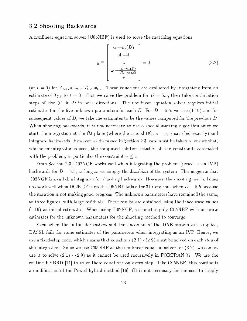
3.2 Shooting BackwardsA nonlinear equation solver (C05NBF) is used to solve the matching equationsg � 26666666664 u� us(D)A� 1�! � D�us(D)Rs(xCJ ;d)x 37777777775 = 0 (3:2)(at t = 0) for ACJ ; d; �CJ ; TCJ ; xCJ . These equations are evaluated by integrating from anestimate of TCJ to t = 0. First we solve the problem for D = 5:5, then take continuationsteps of size 0.1 in D in both directions. The nonlinear equation solver requires initialestimates for the �ve unknown parameters for each D. For D = 5:5, we use (1.19) and forsubsequent values of D, we take the estimates to be the values computed for the previous D.When shooting backwards, it is not necessary to use a special starting algorithm since westart the integration at the CJ plane (where the crucial BC, u = c, is satis�ed exactly) andintegrate backwards. However, as discussed in Section 2.3, care must be taken to ensure that,whichever integrator is used, the computed solution satis�es all the constraints associatedwith the problem, in particular the constraint u � c.From Section 2.3, D02NGF works well when integrating the problem (posed as an IVP)backwards for D = 5:5, as long as we supply the Jacobian of the system. This suggests thatD02NGF is a suitable integrator for shooting backwards. However, the shooting method doesnot work well when D02NGF is used: C05NBF fails after 31 iterations whenD = 5:5 becausethe iteration is not making good progress. The unknown parameters have remained the same,to three �gures, with large residuals. These results are obtained using the inaccurate values(1.19) as initial estimates. When using D02NGF, we must supply C05NBF with accurateestimates for the unknown parameters for the shooting method to converge.Even when the initial derivatives and the Jacobian of the DAE system are supplied,DASSL fails for some estimates of the parameters when integrating as an IVP. Hence, weuse a �xed-step code, which means that equations (2.1) - (2.9) must be solved on each step ofthe integration. Since we use C05NBF as the nonlinear equation solver for (3.2), we cannotuse it to solve (2.1) - (2.9) as it cannot be used recursively in FORTRAN 77. We use theroutine HYBRD [11] to solve these equations on every step. Like C05NBF, this routine isa modi�cation of the Powell hybrid method [16]. (It is not necessary for the user to supply23

the Jacobian.) HYBRD behaves similarly to C05NBF when applied to (2.1) - (2.9); we takethe initial estimate for u1 to be 99% of u0 so that HYBRD computes a solution such thatu � c.When we use (1.19), our code converges to the same solution (to six �gures) as thatobtained by solving the problem using the code [6] for D = 5:5. Next we take continuationsteps of size 0:1 in D. The results are given in Table C.4 of [17] and are plotted in Figure2. The computed values of dc and Dc are 8.8314 (to �ve signi�cant �gures) and 3.09 respec-tively. We can integrate successfully for D�[2:6; 6:8] using continuation steps of size 0.1. Byreducing the continuation step size to 0.01, we can extend the range for D to [2.51, 6.92] (wealso determine Dc and dc by taking continuation steps of this size). It is possible to takecontinuation steps of size 0.5 when increasing D (the last successful value of D is 6.5) and ofsize 0.7 when decreasing D (the last successful value of D is 2.7). In contrast, in the ODEapproach, Braithwaite et al. [6] took continuation steps of size 0.9 in both directions, whileBeardah and Thomas [4] stepped directly from D = 5:5 to D = 2:7 and to D = 6:7.At either end of the range of D, when the code fails it does so after several iterations ofC05NBF. When this occurs, the values of the unknown parameters computed by C05NBFare such that the integrator fails shortly after the start of the integration. When we solvethe quintic in un at this time point, we �nd that no root is valid: roots 1, 2, 3 violate theconstraints and roots 4, 5 are complex conjugates with small imaginary parts. The realpart is approximately equal to the value of c(p; v; �) on the previous step. For most D, thesolution to which C05NBF converges is such that the constraints A � 1; � � 0 are violatedby a small amount (typically of the order 10�10) at t = 0. Since the BCs at t = 0 giveA(0) = 1 and �(0) = 0, we accept this as numerical error. No other constraints are violatedby the computed solution. The results agree with those given in [6] to at least four �guresand to those given in [4] to at least three �gures. The computed values Dc; dc agree withthose of [4, 6] to three �gures. These values of Dc; dc agree with those obtained by shootingforwards to one signi�cant �gure.4. Future WorkThere are two main areas for future work. One is to incorporate a tailored variable-order,variable-step integrator into our shooting codes. As discussed above, the algorithm mustselect the correct root, particularly on the �rst step of the integration, for the required24

solution to be computed. When shooting forwards, the code must deal e�ectively with thesingularity at TCJ . However, shooting forwards presents such di�culties that it may notbe worthwhile. Although developing a variable-order variable-step integrator would be alengthy process, we would not anticipate further di�culties than when using a �xed-stepintegrator.The other main area of research is to use shooting to solve the functionally complexmodel of detonation posed as a DAE. This di�ers from the simple model in that thefunctions F (�; p); R(x; xCJ ; d);H(p; v; �); us(D); c(p; v; �); �(p; v; �; c) are highly nonlinear.Many more constants are introduced, which depend on the type of explosive used. However,the number of unknown parameters remains the same. The complicated model problem alsohas index one, except at t = TCJ , where the index is two. As for the simple model, di�eren-tiating the system twice at TCJ leads to a quadratic in u0. The constraint u � c enables oneto decide which root gives the required solution.Zhang and Gladwell [19] solved the functionally complex model by reformulating it as asystem of �ve ODEs and shooting forwards. They show that on its lower branch, the solutionmay bifurcate to another solution curve. In [20] they show that this behaviour may arisein other singular free boundary value problems by examining an ODE test problem whichshares some of the properties of the detonation problem. Beardah and Thomas [5] solvedthe complicated model as well as the simple one (both posed as implicit DAEs) using theirown collocation code. They also found another solution for the lower branch of the solutioncurve. Their results match those produced in [19] (to graphical accuracy). Braithwaite etal. [7] solved the functionally complex model posed as an explicit system of nine ODEsby shooting backwards. Their results agree (to graphical accuracy) with those of [5, 19],although their solution curve stops short.The ideal method of solution for the functionally complex problem would be to shootforwards, solving the model in its original implicit DAE formulation. When the k-step BDFis applied to the problem, we can reduce the resulting system to the solution of one equationin un. Unlike the simple model of detonation, however, this equation is not a polynomial.Appropriate initial estimates must be supplied to this equation solver; using the forwardEuler method to evaluate these estimates yields a quartic in u1 (rather than a quadratic inu1, as for the simple model). Neither D02NGF nor DASSL gives a solution which satis�esthe constraints. As long as suitable initial estimates are supplied to the nonlinear equationsolver used in implementing the k-step BDF, we would expect shooting backwards to work25

for the implicit DAE formulation.References[1] Ascher U.M., Christiansen, J. and Russell R.D., Collocation software for boundary valueODEs, ACM Trans. Math. Soft., 7 (1981) 209-222.[2] Ascher U.M. and Spiteri R.J., Collocation software for boundary value di�erential-algebraic equations, SIAM J. Sci. Comp. 5 (1994) 938-952.[3] Beardah C.C., Finite Di�erence Solution of Di�erential/Algebraic Equation Bound-ary Value Problems Arising in the Modelling of Uncon�ned Detonations, Ph.D. Thesis,UMIST (1991).[4] Beardah C.C. and Thomas R.M., Finite di�erence solution of a singular index one di�er-ential/algebraic equation boundary value problem arising in the modelling of uncon�neddetonations, Math. Eng. Ind. 3 (1991) 215-228.[5] Beardah C.C. and Thomas R.M., Two mathematical models of uncon�ned detonationand their numerical solution, Circuits Systems Signal Process. 13 (1994) 155-165.[6] Braithwaite M., Farran T., Gladwell I., Lynch P.M., Minchinton A., Parker I.B. andThomas R.M., A detonation problem posed as a di�erential/algebraic boundary valueproblem, Math. Eng. Ind. 3 (1990) 45-57.[7] Braithwaite M., Farran T., Gladwell I., Lynch P.M., Minchinton A., Parker I.B. andThomas R.M., Private Communication (1994).[8] Brenan K.E., Campbell S.L. and Petzold L.R., Numerical Solution of Initial-Value Prob-lems in Di�erential-Algebraic Equations, SIAM (1996).[9] Clark K.D. and Petzold L.R., Numerical methods for di�erential-algebraic equations inconservative form, Report No. UCRL-JC-103423, Lawrence Livermore National Labo-ratory, California (1990).[10] Fickett W. and Davis W.C., Detonation, University of California Press (1979).26

[11] Garbow B.S., Hillstrom K.E. and Mor�e J.J., Testing unconstrained optimization soft-ware, ACM Trans. Math. Soft. 7 (1981) 17-41.[12] Kirby I. and Leiper G., A small divergent detonation theory for intermolecular explo-sives, Proceedings of the Eighth (International) Symposium on Detonation, Albuquerque(1985).[13] Lynch P.M., Private Communication (1996).[14] The NAG Fortran 77 Library Manual - Mark 19. The Numerical Algorithms GroupLimited, Oxford (1999).[15] Nasiruddin N., Private Communication (1999).[16] Powell M.J.D., A hybrid method for nonlinear algebraic equations. In : NumericalMethods for Nonlinear Algebraic Equations (Edited by P. Rabinowitz). Gordon andBreach (1970).[17] Sturgeon J.A., A Shooting Technique for a Di�erential/Algebraic Boundary Value Prob-lem Arising in Detonation Modelling, Ph.D. thesis, UMIST (1997).[18] Zhang W. and Gladwell I., Analysis of a simpli�ed detonation problem.Math. Eng. Ind4 (1993) 1-11.[19] Zhang W. and Gladwell I., Bifurcation phenomena in a detonation problem, Appl.Numer. Math. 9 (1992) 427-445.[20] Zhang W. and Gladwell I., Bifurcation phenomena in singular free boundary valueproblems, Appl. Numer. Math. 10 (1992) 149-158.27