Numerical modelling and graph theory tools to study ecological connectivity in the Great Barrier Reef

Page 1

Nc

CVa

Bb

c

d

Le

B

a

ARRA

KLMCGGC

1

vkt(eailibt

0h

Ecological Modelling 272 (2014) 160– 174

Contents lists available at ScienceDirect

Ecological Modelling

jo ur nal home p ag e: www.elsev ier .com/ locate /eco lmodel

umerical modelling and graph theory tools to study ecologicalonnectivity in the Great Barrier Reef

hristopher J. Thomasa,∗, Jonathan Lambrechtsa, Eric Wolanskic, Vincent A. Traagd,incent D. Blondeld, Eric Deleersnijdera,e, Emmanuel Hanertb

Université catholique de Louvain, Institute of Mechanics, Materials and Civil Engineering (iMMC), Avenue G. Lemaître 4-6, B-1348 Louvain-la-Neuve,elgiumUniversité catholique de Louvain, Earth and Life Institute (ELI), Croix du Sud 16, B-1348 Louvain-la-Neuve, BelgiumJames Cook University, TropWATER and School of Marine and Tropical Biology, James Cook Drive, Townsville, Queensland 4811, AustraliaUniversité catholique de Louvain, Institute of Information and Communication Technologies, Electronics and Applied Mathematics (ICTEAM), Avenue G.emaître 4-6, B-1348 Louvain-la-Neuve, BelgiumUniversité catholique de Louvain, Earth and Life Institute (ELI), Georges Lemaître Centre for Earth and Climate Research (TECLIM), Place Louis Pasteur 3,-1348 Louvain-la-Neuve, Belgium

r t i c l e i n f o

rticle history:eceived 26 March 2013eceived in revised form 2 October 2013ccepted 4 October 2013

eywords:arval dispersalarine connectivity

oral

a b s t r a c t

The process of coral larval dispersal is important for coral reef ecosystems, but remains poorly under-stood and hard to gauge. Better knowledge of inter-reef connectivity patterns would be useful in enablingbetter management of coral reef waters however. By employing a spatially explicit numerical mod-elling approach, we simulate larval dispersal through the central section of the Great Barrier Reef (GBR),comprising over 1000 reefs, and identify spatial patterns in the inter-reef connectivity network using acommunity detection method from network science. This paper presents the modelling approach usedand discusses the significance of the results.

Inter-reef connectivity networks were estimated for 4 different coral species, and significant differences

reat Barrier Reefraph theoryommunity detection

between them were found. We show how we can partition reefs into clusters, or “communities”, thatare sparsely connected with each other, and therefore identify important barriers to larval dispersal. Byfine-tuning a resolution parameter in the community detection method, we can find dispersal barriers ofvarying strength. Finally, we show that the average connectivity length scale varies significantly acrossthe different reef communities, and suggest that this may have repercussions for the optimal placementof marine protected areas (MPAs) to maximise connectivity with surrounding reefs.

© 2013 Elsevier B.V. All rights reserved.

. Introduction

For most types of coastal marine species, the process of lar-ae dispersing through the ocean prior to reaching adulthood –nown as the pelagic larval phase – is vital in enabling popula-ion exchange between geographically separated sub-populationsCowen and Sponaugle, 2009; Cowen et al., 2006). In coral reefcosystems the pelagic larval phase takes on an added importances marine life is predominantly concentrated onto reefs of vary-ng size separated by open sea. Many species of reef fish nevereave their home reef as adults (Jones et al., 2009), whilst coral

s physically fixed to the reef surface and is thus unable to traveletween reefs. It is therefore only during the pelagic larval phasehat these species can spread to new reefs, repopulate damaged

∗ Corresponding author. Tel.: +32 10478031.E-mail address: [email protected] (C.J. Thomas).

304-3800/$ – see front matter © 2013 Elsevier B.V. All rights reserved.ttp://dx.doi.org/10.1016/j.ecolmodel.2013.10.002

reef populations and maintain a healthy gene pool by exchang-ing larvae between separate sub-populations (Buston et al., 2012).Understanding how larvae disperse, where they can disperse to,and how resilient this process is to environmental change is essen-tial to understanding the dynamics – and resilience – of coral reefecosystems. Conservation strategies for coral reefs often involvethe designation of Marine Protected Areas (MPAs) in which localanthropogenic interference is limited. In order for reefs in MPAnetworks to be effective in replenishing coral and reef fish popula-tions in neighbouring reefs, the size and spacing of MPAs shouldaccount for the dispersal potential of marine species present inthe region (Largier, 2003; Munday et al., 2009; Olds et al., 2012),which is not currently the case for most major coral reef ecosys-tems (Jones et al., 2009; Almany et al., 2009). Whilst some recent

studies have proposed MPA designs which incorporate connectivityestimates to improve conservation performance, e.g. Mumby et al.(2011), Guizien et al. (2012), a major stumbling block so far hasbeen a lack of location-specific knowledge of larval dispersion and

Page 2

l Mode

cmfi

modtsiuvtrelap2

iccto0mhaeietiecittb

vttictbi2tcozelflgrair

w

C.J. Thomas et al. / Ecologica

onnectivity patterns (Drew and Barber, 2012). Spatially explicitodelling studies such as the one presented in this article aim to

ll this knowledge gap.Larval dispersal remains very difficult to directly observe or

easure, due to the small size of the larvae, the vastness of thecean, and the fact that dispersion can occur over time-scales ofays to weeks (Drew and Barber, 2012). Genetic tools can be usedo measure the level of genetic connectivity between two givenub-populations, however these tools, whilst useful in quantify-ng present-day and historical connectivity, are by their naturenable to explain the processes driving the dispersion of lar-ae or to predict future trends (Palumbi, 2003), and are unableo provide spatially continuous detailed information over largeegions. Numerical modelling tools can be used to fill this knowl-dge gap, both by providing large-scale estimates of present-dayarval dispersion and connectivity patterns, and by showing how

change in physical or biological factors driving the dispersionrocess could alter inter-reef connectivity patterns (Werner et al.,007).

The transport of larvae between separate reefs can be describedn terms of “ecological” (or demographic) connectivity, which con-erns the movement of individual larvae, or in terms of “genetic”onnectivity, which concerns the exchange of genetic informa-ion. Ecological connectivity occurs over the time- and space-scalesver which most larvae disperse (typically days to weeks and.1–100 km for coral) and is of primary interest for fisheries, reefanagement and MPA planning. Genetic connectivity on the other

and is a more complex process which plays out over many gener-tions, with time- and space-scales spanning a greater range thancological connectivity. For instance, the migration of just a fewndividuals per generation between two sub-populations can benough to prevent genetic differences from developing, and canherefore represent a genetically significant level of connectiv-ty (Cowen and Sponaugle, 2009; Leis et al., 2011), despite beingcologically insignificant. It is not a straightforward exercise toompare observed genetic connectivity with ecological connectiv-ty predicted using large-scale numerical models as these modelsypically do not have enough precision to estimate transport downo ecologically insignificant (but still genetically significant) num-ers of larvae, over time periods in the order of years.

In this paper we present a modelling approach to simulate lar-al dispersal down to reef-scale spatial resolution, and use thiso study ecological connectivity in the region covering the cen-ral section of the Great Barrier Reef (GBR) in Australia, whichncludes roughly 1000 reefs. The GBR is a region with a particularlyomplex bathymetry and a correspondingly complex water circula-ion (Wolanski, 1994). Small-scale circulation at the reef-scale haseen shown to interact significantly with large-scale circulation, for

nstance through the ‘sticky water’ effect (Wolanski and Spagnol,000; Wolanski et al., 2003; Andutta et al., 2012). In order to cap-ure all major scales of motion, it is therefore necessary to resolveurrents down to the reef scale: 100 m to 1 km. Present-day modelsf circulation in the GBR and other reef areas tend to have a hori-ontal resolution of 1–2 km however (e.g. Luick et al., 2007; Parist al., 2007), too large to explicitly resolve flow at the lower range ofarval dispersion length-scales, or even to capture many significantow features in the reef-dense GBR. The use of nested structuredrids is unfeasible in the GBR as the areas requiring enhancedesolution would be too numerous. In this study we instead use

finite element ocean model, SLIM,1 to model water circulationn the GBR using an unstructured grid. This allows us to achieveeef-scale resolution around reefs at an acceptable computational

1 Second-generation Louvain-la-Neuve Ice-ocean Model; seeww.climate.be/slim for more information.

lling 272 (2014) 160– 174 161

cost (Lambrechts et al., 2008). We then employ an Individual BasedModel (IBM) to simulate the dispersion and settling of coral larvaethrough the domain.

Large-scale spatially-explicit simulations such as this can pro-duce a huge amount of data, so a set of tools is needed to interpretthis output if we are to draw useful conclusions. A number ofmathematical tools have been developed to study properties ofnetworks, including biological and ecological networks of geo-graphically separate, connected populations (Proulx et al., 2005).The use of these tools in studies of coral connectivity has so farbeen limited however. Treml et al. (2008) showed how graphtheory can be used to investigate dispersal pathways and iden-tify ‘stepping-stone’ islands linking distant populations and, morerecently, Kininmonth et al. used a graph theoretical approach toexplore the robustness and scale (Kininmonth et al., 2010b) of a reefnetwork, as well as spatial clustering of connections (Kininmonthet al., 2010a). Nilsson Jacobi et al. (2012) used community detectiontools to identify sub-populations in a network of marine habitatsfor generic sessile invertebrates in the Baltic Sea, and to infer thepresence of dispersal barriers. They also investigated how manyclusters contained MPAs, and concluded that MPAs were poorlydistributed amongst the clusters.

In the present study we explore the use of a graph theoreticalapproach to identify spatial patterns in large-scale connectivity ofcoral larvae. We use a community detection method to identifyclusters of reefs which are ecologically isolated from each other,and we partition the central section of the GBR into such clusters,known as “reef communities”. Each reef community can be seenas a self-contained ecological sub-region, with little or no larvaeexchanged with reefs in other communities. We establish mapsdelimiting separate reef communities in the GBR for 4 differentspecies of coral, and find that significant inter-species differencesexist in the size and shapes of the communities. These differencescan be explained by variations in the biological characteristics ofeach species, and in particular their pre-competence periods. Wealso explore the differences in connectivity length scales across thedifferent communities, and compare these to average MPA spacing.Such findings can potentially be used to inform the placement andspacing of MPAs to better take into account the different connec-tivity potential of larvae in each ecological sub-region.

This study has some parallels with Nilsson Jacobi et al. (2012), inwhich a similar graph theoretical approach to identify communitiesof generic sessile invertebrates in the Baltic Sea. Some differencesof implementation between the two approaches are discussed inSection 2.3.2. No study that we are aware of has used these toolsto compare the connectivity patterns of different marine specieshowever, or to investigate whether dispersal patterns vary signif-icantly in different sub-populations and how community-specificdispersal distances compare with MPA spacing.

2. Methods

The numerical modelling approach presented in this paper canbe broadly divided into three stages: (1) modelling the hydrody-namics of the region, (2) simulating the transport of larvae, and (3)interpreting the model output. Each stage is now discussed, and aflow-chart summarising this process is presented in Fig. 2.

2.1. Resolving the hydrodynamics

2.1.1. Oceanographic model

Given the highly multi-scale nature of the water circulation

in the GBR (as discussed in Section 1), it is important to use anocean model able to cope with a large range of length scales. Weused the finite element, unstructured-grid ocean model SLIM, in its

Page 3

1 l Mod

deubiamrn2flcm

dGvA2S

osorptad

2

eu

wvc�

LdPgwTtrr(wulm

retay

The virtual larvae were released over all of the shallow-waterreefs in the domain of interest. The number of larvae released overeach reef was a proportional function of the reef’s surface area, with

62 C.J. Thomas et al. / Ecologica

epth-integrated, barotropic version. SLIM is ideally suited to mod-lling water circulation in coastal and multi-scale regions due to itsse of an unstructured grid, which allows the model resolution toe varied in space (Legrand et al., 2006). The grid used in this study

s shown in Fig. 3. The element size varies from 400 m close to reefsnd coastlines to 10 km in deeper ‘open-sea’ areas. This allows theodel to explicitly capture small-scale circulation features through

eef passages and around islands, which are known to have a sig-ificant impact on large-scale circulation (Wolanski and Spagnol,000), whilst using a coarser resolution in ‘open-sea’ areas whereow is known to be more uniform. This modelling approach allowsomputational resources to be focused to where they are neededost.The SLIM model has already been shown to be capable of repro-

ucing important small- and large-scale circulation features in theBR by Lambrechts et al. (2008), and has been used and validated inarious studies of the hydrodynamics and ecology of the GBR (e.g.ndutta et al., 2011, 2012; Hamann et al., 2011; Wolanski et al.,013) and other coastal oceans and estuaries around the world (e.g.assi et al., 2011; de Brye et al., 2010).

Whilst this study focuses on larval dispersal in the central thirdf the GBR, from just north of Townsville (18.7◦ S) down to justouth of Broad Sound (22.5◦ S), the grid covers the entire coastalcean of the GBR from 11◦ S down to 25.5◦ S, but with a loweresolution in the northern and southern thirds, where larval dis-ersion is not simulated. This is to allow the boundary conditionso be imposed at the shelf break where the data are more reliable,nd has very little effect on the computational cost of simulationue to the low resolution outside of the central third of the GBR.

.1.2. Governing equations, forcings and paramaterisationsSLIM was used to solve the depth-integrated shallow water

quations to calculate the water elevation � and the current velocity:

∂�

∂t+ ∇ · (Hu) = 0 (1)

∂u

∂t+ (u∇) · u = −fez × u − g∇� − CD|u|u + �

�H+ 1

H∇ · [H�(∇u)]

(2)

here H is the water column depth, f is the Coriolis factor, ez is a unitector pointing vertically upwards, CD is the bottom stress coeffi-ient, � is the surface wind stress, g is the gravitational acceleration,

is the water density and � is the horizontal eddy viscosity.The model was set up in a similar way to that described by

ambrechts et al. (2008) and Andutta et al. (2011). The bathymetryata used were from the 100 m resolution dataset produced byroject 3DGBR (Beaman, 2010). The bottom stress coefficient isiven as CD = g/(C2H), with the Chezy coefficient C = H1/6/n, andhere the Manning coefficient used was n = 2.5 × 10−2 m1/3 s−1.

his value was multiplied by 10 over shallow reefs to account forhe increased roughness of reef surfaces. The positions of shalloweefs in the GBR were taken from the global distribution of coraleefs provided by the Great Barrier Reef Marine Park AuthorityGBRMPA, 2007). The reefs are not considered emergent and haveater over them at all times. Smagorinsky’s paramaterisation wassed to account for unresolved turbulent features and boundary

ayer effects around coastlines and islands, with horizontal kine-atic eddy viscosity dependent on the local grid element size.The external forcings applied to the model consisted of tides and

esidual currents at the open-sea boundaries and wind over the

ntire domain. Tidal forcing was applied at the boundaries usinghe OSU TOPEX/Poseidon Global Inverse Solution dataset (Egbertnd Erofeeva, 2002), whilst wind data extracted from NCEP reanal-sis was provided by NOAA/OAR/ESRL PSD (Kalnay et al., 1996). The

elling 272 (2014) 160– 174

wind stress acting on the sea surface was modelled using the para-materisation proposed by Smith and Banke (1975). The effect of theEast Australian Current was accounted for by imposing a constantresidual flow into the domain at the boundary with the Coral Seabetween 15.0◦ S and 17.6◦ S, and allowing this water to flow outthrough the southern and northern open-sea boundaries, followingthe same approach as Brinkman et al. (2001). The hydrodynamicswere validated using observed oceanographic elevation and cur-rent data. This validation is presented and discussed in Appendix A.

2.2. Biophysical particle transport

The dispersal and settlement of larvae was modelled by consid-ering millions of “virtual larvae” released into the domain asautonomous, buoyant, individual organisms, passively transportedby the ocean currents and subject to some very simple biologicalprocesses. This is a type of individual based model (see Grimm et al.,2006 for an introduction to IBMs).

Transport of larvae was modelled using a random walk formula-tion of the 2D advection-diffusion equation2 as outlined in Spagnolet al. (2001) and Hunter et al. (1993). The equations used were:

xn+1 = xn + vn�t + Rn√r

√2K�t (3)

vn =(

u + K

H∇H + ∇K

)|xn (4)

where xn and xn+1 are the particle positions at time iterations n andn + 1, respectively, �t is the time difference between iterations, Rn

is a horizontal vector of zero-mean random numbers with variancer, K is the horizontal diffusivity coefficient, H denotes water depthand u is the depth-averaged horizontal water velocity supplied bythe ocean model. The time step used for the simulations in thisstudy was set to �t = 90 s. The horizontal diffusivity coefficient, K,was calculated using the paramaterisation presented in de Bryeet al. (2010), which makes use of the formula of Okubo (1971) tointroduce a dependence on the local hydrodynamic grid elementsize. This approach has been used in numerous studies of coastalseas and estuaries using multi-scale models (e.g. see Lambrechtset al., 2008; Andutta et al., 2011; de Brauwere et al., 2011; Hamannet al., 2011).

The advantages of modelling larval transport with an IBM are:(1) that we can know the start and end points of each larvareleased into the domain, and therefore directly measure the rela-tive strength of larval exchange between every pair of reefs, and (2)that we can directly simulate age- and location-specific processestaking place on larvae (e.g. mortality, acquisition/loss of compe-tence).

The particle-tracker used in this study also modelled two simpleage-related biological processes taking place on the virtual larvae:mortality and acquisition/loss of competence, and these were mod-elled as described by Connolly and Baird (2010), with the mortalityrate being either constant or taken from a Weibull distribution,depending on the species, and the onset and loss of competencemodelled as a gradual process governed by fixed competence acqui-sition and loss rates. A larva was only considered capable of settlingonto a reef whilst it was competent. The values of the parametersused in this study were based on the experimental observations ofConnolly and Baird (2010).

2 (∂/∂t)(Hc) + ∇ · (uHc) = ∇ · (HK ∇ c) where t is time, c is depth-integrated tracerconcentration, H is water depth, u is the depth-averaged horizontal water velocityand K is the horizontal diffusivity coefficient.

Page 4

l Mode

gtcer

2

ibsonp

issb

2

aucr

•

•

•

2

wcwtcb

igpntnb

rltra

C.J. Thomas et al. / Ecologica

reater numbers of larvae released over larger reefs. They were thenracked for the duration of the simulation. Once a larva had acquiredompetency, it was considered to settle onto the first reef it trav-lled over. As soon as a larva settled onto a reef it was immediatelyemoved from the remainder of the simulation.

.3. Extracting useful information

The output of the biophysical model is a large connectiv-ty matrix whose elements give the strength of the connectivityetween every pair of reefs in the domain, where the connectivitytrength is at this point defined as the number of larvae releasedver the source reef which settled onto the sink reef. Thus the con-ectivity matrix encapsulates all of the relevant output from thearticle tracking simulation.

Given the large number of reefs in the domain (over 1000), find-ng useful information from this matrix is a challenge in itself. Thetrategies employed can be broadly divided into two categories:tatistical analysis and identifying spatial patterns. These will nowe outlined in turn.

.3.1. Statistical analysisWe can define some appropriate statistical quantities to char-

cterise connectivity patterns within a given region. These can besed both to describe connectivity in the whole domain, and toompare the connectivity patterns seen in various well-chosen sub-egions.

Weighted connectivity length: the characteristic length scale ofconnectivity between reefs. It is calculated as:∑

all connections connection strength × connection length∑all connections connection strength

(5)

where the connection strength is given by the number of larvaereleased over the source reef that settled onto the sink reef, whilstthe connection length is the radial distance between source andsink reefs.Proportion of self-recruitment: the proportion of connectionsfor which the source and sink reefs are the same.Average plume length: the furthest distance from the source reefat which connections occur, averaged over all connections. Thisis an indication of how far away a typical reef’s influence extends.

.3.2. Identifying spatial patternsAnother way of characterising the connectivity of the reef net-

ork is to look for spatial patterns. It would be useful to identifylusters of reefs which are strongly connected to each other, buteakly connected to reefs outside of their cluster. By partitioning

he GBR reef network into such clusters we can identify ecologi-ally separate groups of reefs, and therefore infer the presence ofarriers to larval dispersion between these groups.

We propose a graph theoretical approach to partition the GBRnto reef clusters. The GBR can be cast as a directional, weightedraph by considering its reefs as nodes in the graph, and the trans-ort of larvae between reefs as connections, or “edges”, linking theodes. The strength of each edge, known as its “weight”, is given byhe connection strength between the two nodes it connects (i.e. theumber of larvae travelling from one node to the other), denotedy wij for an edge linking source reef i to sink reef j.

One particularity of this graph is that an edge linking two smalleefs will have a much smaller weight than an edge linking two

arge reefs, as fewer larvae are released over the small reefs duringhe simulation. Connections between larger reefs then play a largerole than connections between smaller reefs, even where they onlyccount for a small fraction of the total larvae released over the

lling 272 (2014) 160– 174 163

source reef. We mitigate this problem by normalising the edgeweight by an appropriate quantity to make it “non-dimensional”;we chose to normalise the edge weight wij by the total number oflarvae released at reef i (that have settled somewhere), denoted bysi. We thus arrive at the normalised edge weight Aij = wij/si. The neteffect is to increase the importance of edges between small reefs,which would otherwise be dwarfed by the edges between the largerreefs.

The aim is then to partition this graph into a number of coherentclusters, known as communities, whose members are strongly con-nected with each other and weakly connected to the other nodes inthe network. Many methods have been developed in recent yearsto partition a graph into communities (see Fortunato, 2010 for anextensive review). One of the most popular methods has been tooptimise a quantity called “modularity”, which is a measure of howstrongly a graph is divided into clusters compared to a randomgraph (Newman and Girvan, 2004). A significant drawback of thismethod is that it suffers from a resolution limit (Fortunato, 2007),meaning that communities smaller than a certain scale (relative tothe size of the graph) cannot be identified. In addition, the ecolog-ical significance of communities identified using modularity is notentirely clear, due to the comparison to a random graph.

We therefore chose to use a variant of modularity which doesnot suffer from these problems. Specifically, we employed the con-stant Potts model (CPM) developed by Traag et al. (2011) andRonhovde and Nussinov (2010), which is based on the principle ofcomparing the density of edges within the communities to a con-stant resolution parameter, rather than to a random graph. Morespecifically, if we denote by Sc the set of nodes that belong to acommunity c, we can define by ecd =

∑i∈Sc,j∈Sd

Aij the total weight

between community c and d, and denote by nc the total number ofnodes in community c. CPM is then defined as

H = −∑

c

ecc − �n2c , (6)

where ecc is simply the total weight inside community c, and � is theuser-defined resolution parameter. The minus sign is simply a mat-ter of convention. The goal is to find a partition into communitiesfor which H is minimal. The optimisation of H was carried out usinga modified Louvain Method algorithm (Blondel et al., 2008), follow-ing the approach described in Traag et al. (2011). The CPM approachhas also been used to study the community structure of a marinenetwork by Nilsson Jacobi et al. (2012), who instead used a spectralbased algorithm to optimise the objective function. A comparisonof the performance of this algorithm with the Louvain Method algo-rithm is included in Appendix B. Both methods returned partitionsof similar quality on benchmark networks, and returned similarpartitions for a set of central GBR connectivity networks.

CPM has two principal advantages (Traag et al., 2011). Firstly, itdoesn’t suffer from a resolution limit. Hence, there is no theoreticalsmallest or largest scale beyond which it is unable to identify com-munities. Secondly, the communities have a natural interpretation,which is twofold. First, in an optimal partition, each communityhas an internal connectivity of at least � , i.e. ecc/n2

c ≥� . Second, twocommunities in an optimal partition are separated by a connectiv-ity of at most � , i.e. ecd/ncnd ≤ � . In other words, the communitiesidentified by the algorithm should have the two following proper-ties:

Inner connectivity The average connection strength betweenmembers of the same community is greater

than � .

External connectivity The average connection strength betweenany two reefs in different communities is lessthan � .

Page 5

1 l Mod

Tttclwmhmii

vvwGtrbowm

bcaiudciopttsbc

gpdtfsctctUr

3

pLcrgtts4v

64 C.J. Thomas et al. / Ecologica

his approach allows us to detect reef communities at different spa-ial scales. If we use a low value of � , the connectivity between anywo communities will be small (i.e. we have nearly impermeableommunity boundaries), but the internal connectivity may also beow and the size of the communities will tend to be large. If instead

e use a higher value of � , the connectivity between any two com-unities may be higher, but the internal connectivity will also be

igher and communities will tend to be smaller and boundariesore permeable. The � value is therefore an indication of how much

nter- and intra-community connectivity there is. This concept isllustrated in Fig. 4.

This naturally leads to the question of how to find the “optimal”alue of the resolution parameter, � . In reality there is no “optimal”alue: the size of the value used clearly depends on what questione want to answer. Imposing a small value of � will partition theBR into a small number of large, weakly connected communi-

ies. This will allow us to identify the most ecologically isolatedeef communities, and will therefore allow us to find the strongestoundaries to larval dispersion in the GBR. Imposing a higher valuef � will allow us to identify smaller communities which may existithin the boundaries of the larger communities, and thus identifyore localised or weaker barriers to dispersion.A sensitivity analysis is carried out to identify how (1) the num-

er of communities and (2) the percentage of inter-communityonnectivity vary over a range of � values. An example of such

sensitivity analysis, showing the variation of the proportion ofnter-community connectivity with � , is shown in Fig. 5. This fig-re illustrates how the inter-community connectivity increases inistinct steps as � is increased. Each jump in the curve generallyorresponds to a significant change in the community partitionsdentified by the algorithm. Between two jumps there are plateauxf relatively stable connectivity over some interval [�1, �2]. Largerlateaux then correspond to especially pertinent partitions, sincehe external connectivity will in general be lower than �1 whilsthe internal connectivity will be higher than �2. We then choose aelection of values of � for which these variables are relatively sta-le, indicated by the asterisks in Fig. 5, and compare the communityonfigurations obtained using each of these values.

Since boundaries to larval dispersion generally arise due to topo-raphic features or between areas with distinct water circulationatterns, we can reasonably expect that the characteristics of larvalispersion in each community may be distinct from each other. Weherefore calculate the statistical quantities defined in Section 2.3.1or each reef community and compare them, to see if there is aignificant variation in connectivity length-scales in the differentommunities. If, for a given value of � , all of the communities iden-ified have similar connectivity length-scales then we will generallyhoose to ignore that particular configuration, as it does not iden-ify communities with significantly different connectivity patterns.ltimately the goal is to identify the configurations which partition

eefs into communities with physically distinct dispersal patterns.

. Results and discussion

Virtual larvae were released over all reefs in an area encom-assing the central GBR – roughly one-third of the GBR’s total area.arval dispersion was simulated for 4 different species of broad-ast spawning larvae for which mortality and settling data wereeadily available: Goniastrea retiformis, Acropora gemmifera, Platy-yra daedalea and Acropora millepora. All four species are knowno be present in the GBR. The oceanographic forcings used were for

he period of December 2007, corresponding to a typical coral masspawning period, and the positions of the larvae were tracked for

weeks. After this period the proportion of larvae still alive wasery small (<4% for all species). Whilst variations in oceanographic

elling 272 (2014) 160– 174

conditions between successive annual spawning seasons may mod-ify larval dispersal patterns year-on-year, we chose to focus on onesingle season, as the scope of this paper is not to provide yearly esti-mates of dispersal patterns but rather to develop tools which can beused to study connectivity patterns for any given spawning season.

3.1. Dispersal statistics

The graph showing connection strength against distance for thedifferent species studied is shown in Fig. 7. Inter-species differ-ences in dispersion potential are clearly visible. Table 1, showingthe global connectivity statistics, provides some additional detail.The proportion of larvae self-recruiting varies significantly betweenspecies, from 55% for G. retiformis to 18–19% for A. gemmifera andP. daedalea and down to only 13% for A. millepora. This difference isexplained by the fact that the latter three species have much longeraverage pre-competency periods than G. retiformis: their larvaetypically start to acquire competence after 3–4 days, whereas lar-vae of G. retiformis start to become competent immediately, and soare more likely to settle close to their release site. This is shown inFig. 6, which shows the proportion of larvae alive and competentduring the simulations. The later this curve peaks, the longer theaverage pre-competence periods, and so the longer the period dur-ing which the larvae can be advected and diffused away from theirnatal reef prior to settlement.

The typical length-scales over which most connectivity occurstell a similar story to the self-recruitment statistics: G. retiformislarvae settle closer to their natal reef than the other species, withan average connectivity length of 6 km, whilst A. millepora tend tosettle furthest from their natal reef, with an average connectivitylength of 31 km. Long-distance connectivity (where long-distanceis here defined as >100 km) is marginal in ecological terms for all 3coral species, though not entirely insignificant for A. gemmifera, P.daedalea and A. millepora. Finally, the average plume lengths indi-cate that we would expect to see some minimal larval exchange atdistances of over 80–130 km from the source reef, depending onthe species.

3.2. Spatial patterns for G. retiformis

The community detection method described in Section 2.3.2 wasused to partition the reefs into reef communities. For each speciesa set of different possible partitioning arrangements was gener-ated by varying the value of the resolution parameter, � , through agiven range. A selection of different partitioning arrangements forthe species G. retiformis is given in Fig. 8, showing different parti-tioning arrangements obtained using a low, a medium and a highvalue of � . These correspond to arrangements with low, mediumand high levels of inter-community connectivity respectively. Wewill focus our description on G. retiformis for now, as the effect ofvarying � has a similar effect for the other species. We will subse-quently compare equivalent community configurations obtainedfor different species.

The partitioning arrangement obtained with the lower value of� , shown in Fig. 8a, exhibits a very low level of inter-communityconnectivity – just 0.001%. In other words only 1 in every100,000 settled larvae settled outside of their reef community,so broadly speaking the number of larvae crossing communityboundaries is ecologically insignificant. We can see that the reefsaround the Whitsunday Islands have been grouped together inthe same community as the offshore reefs, as the level of trans-port between the two areas is not entirely insignificant. Perhaps

surprisingly, the group of coastal reefs just south of the Whit-sunday Islands is in a separate reef community, implying thatthe model predicted negligible levels of transport between thetwo communities, despite their geographic proximity. This is

Page 6

C.J. Thomas et al. / Ecological Modelling 272 (2014) 160– 174 165

Table 1Summary of global connectivity characteristics for each species of coral after a 4-week simulation of larval dispersal. For an explanation of each quantity see Section 2.3.1.Average plume length is shown with its standard deviation.

Coral species Self-recruitment (%) Weighted connectivity length (km) Long-distance connectivity (%) Average plume length (km)

G. retiformis 55 6 0.3 80 ± 60P. daedalea 19 20 1.6 117 ± 69

amwsnvtn

oiasapmsbigcar“statrs

winIttncvao

tin(wvaeiotts

A. gemmifera 18 20

A. millepora 13 31

n indication that the “isolation-by-distance” method for esti-ating inter-reef connectivity is not always reliable in areasith complex topography and flow patterns, at least at small

cales. We can also see that the average length of the con-ections within each community, also shown on the diagram,ary significantly from one community to the next. This suggestshat larval dispersion dynamics are different in each commu-ity.

Fig. 8b shows a partitioning arrangement if we increase the valuef the resolution parameter such that inter-community connectiv-ty now accounts for 1% of all connections. The reef communitiesre therefore still ecologically isolated units, as only 1 in every 100ettled larvae crosses a community boundary, but these bound-ries can now be considered to be slightly less rigid. Looking at thisartitioning arrangement, we can see that many smaller-scale com-unity structures exist within the large-scale community structure

hown in Fig. 8a. In particular, the large block of offshore reefs haseen separated from the Whitsunday Islands community, mean-

ng that the “barrier” to dispersal between the Whitsunday Islandsroup and the offshore reefs (which physically corresponds to ahannel of southward-flowing open water), whilst not as significants the “barrier” between the Whitsunday Islands and the coastaleefs south of them seen in Fig. 8a, is still more significant than anybarrier” within the Whitsunday Islands themselves, since these aretill a whole community. It is also revealing that the difference inhe weighted connectivity lengths in the offshore reef communitiesnd in the Whitsunday Islands community is much more significanthan any difference seen in Fig. 8a. This suggests that the differenteef communities identified with this “medium” value of � , andhown in Fig. 8b, have much more distinctive dispersal dynamics.

A partitioning arrangement obtained using a higher value of � , inhich 4% of connectivity crosses community boundaries, is shown

n Fig. 8c. This figure reveals a more complex structure of commu-ities in both the offshore group of reefs and in the Whitsunday

slands group. Most offshore reef communities are inclined alonghe longshore axis suggesting that reefs are better connected alonghis axis rather than along the cross-shelf axis. This is because theet currents act in the south-eastward longshore direction. With aouple of exceptions, most of the offshore reef communities haveery similar average connectivity lengths. This suggests that therere no major differences in the dispersal dynamics amongst theffshore reefs.

It is more interesting however to look at the reefs aroundhe Whitsunday Islands. At the higher � , they have been splitnto three separate communities: one “coastal” community ofearshore reefs, with a very small weighted connectivity length3 km), another “middle” community of reefs with a much greatereighted connectivity length of 22 km, suggesting that some lar-

ae from this community settle far away from their natal reef,nd finally another “external” community of reefs on the outer,astward-facing side of the Whitsunday Islands. Somewhat surpris-ngly, these reefs also have a small weighted connectivity length –

nly 3 km – suggesting that either these reefs are more shelteredhan those in the “middle” community, or else simply that most ofhe larvae released here are lost to sea and don’t find any reefs toettle onto far away.

1.2 112 ± 685.0 131 ± 73

We can gain an insight into the physical processes causing thisdifference by looking at the effects of the water circulation on trans-port around the Whitsunday Islands. Fig. 9 shows the simulateddispersal of particles released at 5 different carefully chosen sitesaround the Whitsunday Islands after 3.5 days and after 1 week.In the simulation used to create these figures, the particles under-went no mortality or settling processes, so we can use these imagespurely as a guide to potential dispersal rather than as a predictionof real dispersal for a given species. We should note that in thespecies-specific simulations, after 3.5 days 93% of G. retiformis hadsettled onto a reef, whilst after 7 days this number was 97%. Thismeans that very few G. retiformis larvae would have dispersed fur-ther from their release point than shown in both figures. It is clearfrom these images that particles released on the eastward-facingexternal side of the Islands tend to stay closer to their release pointand are advected to the open sea where there are no reefs, whilstparticles released in middle section tend to disperse further awayand pass through other reef-dense areas. Furthermore, there is lit-tle mixing between particles released on either side. This explainswhy the two sides are placed in different communities for G. reti-formis, and why the connectivity length scales are so different inthese communities.

In summary, Fig. 8a–c shows different possible partitioningarrangements for G. retiformis, each of which gives us a differentset of information. The question is which is the most useful? Wesuggest that all three are useful in that they complement eachother, and provide us with information about the network overdifferent length scales. Fig. 8a suggests that as a first large-scaleapproximation we should at least treat the coastal reefs south ofthe Whitsunday Islands, and the reefs in Broad Sound, separatelyfrom the other reefs in the domain. Fig. 8b shows that, in additionto this clear separation, there are also very significant differenceson a smaller scale between the dispersal patterns of larvae releasedaround the Whitsunday Islands and those released on the offshorereefs, and finally Fig. 8c shows that the Whitsunday Island reefscan themselves be subdivided into three different areas with dis-tinct patterns of larval dispersion. Depending on the scale at whichwe want to look at the system, we should select a value of gammawhich highlights the information relevant for that scale.

3.3. Spatial patterns for all species

Fig. 10 shows partitioning arrangements for all four speciesstudied, where the percentage of inter-reef connectivity is fixedat around 4% – high enough to see the smaller reef communitiesbut low enough to be ecologically marginal or insignificant. Thisfigure shows that the species with the highest dispersal potentials– primarily A. millepora – form the largest communities, whilst G.retiformis form the smallest communities. This is because A. mille-pora larvae take longer to acquire competence and thus tend totravel further from their natal reef before settling (as reported inTable 1); they are therefore more capable of overcoming physical

barriers to dispersal than other species.

Despite these differences in community size however, we canstill see some patterns recurring for all of the species in thecentral GBR. For instance, the dispersal boundary between the

Page 7

166 C.J. Thomas et al. / Ecological Modelling 272 (2014) 160– 174

Fig. 1. Map of the GBR topography. The coastline is shown to the left, the 200 m-isobath to the right, and reefs are shaded in grey. Triangles show positions ofmoorings used to validate elevation, squares represent moorings used to validatecCC

Wbjg

Feioid

Fig. 3. The oceanographic grid used for simulations. The grid is colour-coded by thelocal characteristic element size – smaller elements are shown in blue and larger ele-ments are shown in red. The element size is a function of water depth and distance

urrents. Legend: LSL: Lizard Island Slope, MYR: Myrmidon Reef, CCH: Capricornhannel, HIS: Heron Island South, LI: Lizard Island, BR: Bowden Reef, OR: Old Reef,U: Cape Upstart, RI: Rattray Island, HO: Hook, BU: Bushy, BE: Bell.

hitsunday Islands and the offshore reefs is always present. The

oundary between the Whitsunday Islands and the coastal reefs

ust south of them is also present for all species, despite theireographical proximity. The typical connectivity length scales also

ig. 2. Flow chart summarising the connectivity modelling process. Input param-ters obtained from observations are shown in ovals, modelling stages are shownn rectangles and outputs are shown in hexagons. Thick arrows represent modelutputs subsequently used as inputs for the next modelling stage. Circled numbersndicate the modelling stages: 1: simulating the hydrodynamics, 2: simulating larvalispersion, 3: extracting useful information.

to the nearest reef. In addition, the element size is further reduced in the central GBRregion. The grid contains roughly 500,000 triangular elements. The western bound-

ary is the North Queensland coastline whilst the northern, eastern and southernboundaries are with the open sea. The box shows grid detail around the Whitsun-day Islands. (For interpretation of the references to color in this figure legend, thereader is referred to the web version of the article.)

vary significantly from one community to another, and tend tobe smaller for nearshore reef communities and larger for offshorecommunities. This suggests that community boundaries often coin-cide with boundaries between areas with different larval dispersaldynamics.

Fig. 10 also reports the average distance between the nearestneighbouring MPAs (GBRMPA-designated “green zones”, or no-take areas) in every community containing 2 or more MPAs. Thesefigures show that MPA spacing does to some extent follow the sametrends as larval dispersal distances; in nearshore areas MPAs tendto be closer together, whilst they tend to be further apart in offshorereef areas. This is positive for promoting connectivity between sep-arate MPAs, as larvae tend to settle closer to their natal reef innearshore areas. One notable exception is in Broad Sound, whereMPA spacing is larger than in other nearshore areas, yet larval dis-persal distances remain small.

For the three species which disperse the furthest (A. millepora,P. daedalea and A. gemmifera), the dispersal distances are not toodissimilar to the MPA spacing,3 suggesting that many MPAs may

3 It is important to bear in mind that the weighted connectivity length reportedis only showing the average distance travelled by larvae; thus some larvae will betravelling further than this, as shown in Fig. 7.

Page 8

C.J. Thomas et al. / Ecological Modelling 272 (2014) 160– 174 167

A B

γ=0.025 γ=0.11

Fig. 4. Example illustrating the role of the resolution parameter � in the community detection method. Diagrams A (left) and B (right) show two identical graphs, withthe circles representing nodes and the lines between them representing connections. These connections all have equal weight. Both graphs have been partitioned usingt nd cow oned um wer c

bstdbdb

4

imdowtph

lbk

Fospt�

he community detection algorithm described in Section 2.3.2, and the thick lines aith the resolution parameter, � = 0.025, whilst the graph in diagram B was partitiaximum connectivity allowed between any two communities, and so results in fe

e ecologically connected to their neighbours. It is notable thatome reef communities do not even contain 2 MPAs, however, par-icularly the smaller communities. For G. retiformis, whose larvaeisperse over smaller distances, typical dispersal distances tend toe much smaller than average MPA spacing, and most communitieso not contain 2 MPAs. This suggests that the level of connectivityetween MPAs is likely to be very species-dependent.

. Conclusions

The process of larvae dispersing through the Great Barrier Reefs controlled by a multitude of factors, both physical (relating to

arine transport) and biological (relating to the behaviour andevelopment rate of the larvae). By using an unstructured-gridcean model as a tool to simulate the ocean circulation in the GBR,e have been able to resolve flow from the large-scale down to

he reef-scale, an essential pre-requisite for modelling larval dis-ersion in the GBR, as this can occur on length-scales ranging fromundreds of metres to hundreds of kilometres.

Using a relatively simple biological model, we have made

arge-scale predictions of larval dispersal using a small num-er of biological parameters, following the best available presentnowledge of larval mortality and development rates as found by

10-6

10-5

10-4

10-3

γ

0

1

2

3

4

5

6

Inte

r-com

munity c

onnectivity %

10 -50.000

0.001

0.002

0.003

0.004

*

*

**

*

**

ig. 5. The percentage of connectivity crossing community boundaries as a functionf the resolution parameter, � for G. retiformis coral larvae. The jumps correspond toignificant changes in the partitioning configuration. The asterisks identify ‘stable’artitioning configurations. The scale is logarithmic in x, as a given interval of � athe lower end of the scale will be more significant, proportional to the local value of, than at the higher end of the scale.

lour-coding demarcate the communities. The graph in diagram A was partitionedsing � = 0.11. Using a lower value of gamma imposes a stronger constraint on the

ommunities being detected.

Connolly and Baird (2010). Whilst this simple model of larvae aspassive massless objects is deemed sufficient to model the trans-port of coral larvae, an increase in model complexity would beessential for modelling fish larvae instead, in particular to accountfor their ability to directionally swim (see Gerlach et al., 2007;Fisher and Bellwood, 2003; Vermeij et al., 2010). This is an areawe plan to study in the future.

We have used a novel strategy to extract useful informationfrom the connectivity matrix by employing a graph theoreticalapproach to identify ecologically separate reef communities. Wehave calculated connectivity characteristics separately for eachreef community, and we have shown that the dispersal poten-tial of larvae in different communities can vary significantly. Wehave provided estimates of dispersal potential in each communityfor 4 different coral species for a given spawning season, and wehave shown that there are significant differences in the dispersalpatterns and potentials between these 4 species. We have also com-pared these community-specific dispersal distances to the averagespacing between neighbouring no-take MPAs in each community,and found that connectivity between MPAs is species-specific, and

that MPA spacing does not always reflect the spatial patterns seenin larval dispersal distances.

In order to translate this approach into practical advice on MPAplacement, the next step should be to quantify the effects of annual

Fig. 6. Graph showing the proportion of larvae that are alive and competent tosettle for each species during the simulation. A greater proportion of G. retiformislarvae are alive and competent in the days immediately after release than any of theother species, which explains their higher self-recruitment rate and lower weightedconnectivity length.

Page 9

168 C.J. Thomas et al. / Ecological Modelling 272 (2014) 160– 174

F ent spb ment

l

voceG

FdC(

ig. 7. Graph showing the connection strength against distance for larvae of 4 differetween source and sink reefs. The x-axis (distance) is cut at 150 km. Self-recruit

ength-scale statistics.

ariation of larval dispersion patterns on the shape and positions

f communities, and on the connectivity characteristics of eachommunity for a given species. Results obtained by Kininmontht al. (2010b) suggest that the dispersal network structure of theBR may undergo significant annual changes, but that stronger

ig. 8. Different reef community configurations for G. retiformis larvae. These different petection method from a low value (a) to a high value (c). The numbers in the white circlesonnections between reefs are shown in light grey for illustrative purposes, with the weakb) G. retiformis; inter-community connectivity: 1%. (c) G. retiformis; inter-community con

ecies of coral, after a 4-week simulation. The distance is measured as radial distanceis not shown in this graph, however it is used to calculate all other connectivity

connections are highly likely to remain in place, at least for the

stretch of the GBR considered in their study. It would also be use-ful to consider a much larger number of different coral species, asit is known that significant inter-species variations in connectivitycan exist (Drew and Barber, 2012), though this may be hampered

artitions were obtained by increasing the resolution parameter in the community show the average weighted connectivity length in each community, in kilometres.er connections filtered out. (a) G. retiformis; inter-community connectivity: 0.001%.nectivity: 4%.

Page 10

C.J. Thomas et al. / Ecological Modelling 272 (2014) 160– 174 169

Fig. 9. Images showing the dispersal of particles released at five chosen sites around the Whitsunday Islands over a week. Particles are colour-coded by release site. Mortalitya c) Pos

tnaf

nd settling were ignored. (a) Initial particle positions. (b) Positions after 3.5 days. (

o some extent by a lack of biological data. Finally more work iseeded to find a way to achieve an “optimal” MPA spacing whichccounts for the different connectivity characteristics of many dif-erent species.

itions after 7 days.

Acknowledgements

This work was carried out under the auspices of ARC grant10/15-028 of the Communauté franc aise de Belgique, “Taking up

Page 11

170 C.J. Thomas et al. / Ecological Modelling 272 (2014) 160– 174

Fig. 10. Equivalent reef community configurations for 4 species of coral larvae. Reefs of the same colour belong to the same community. Black numbers show the weightedc age Mc tions,

( figure

traCBtBd

A

GaDdrhtm1ete(fu

onnectivity length (km) for reefs in each community. Blue numbers show the averonnectivity crossing community boundaries is approximately 4% for all configurac) P. daedalea. (d) A. millepora. (For interpretation of the references to color in this

he challenges of multi-scale marine modelling”. Computationalesources were provided by the Centre de Calcul Intensif et Stock-ge de Masse (CISM) at the Université catholique de Louvain and theonsortium des Équipements de Calcul Intensif en Fédération Wallonieruxelles (CÉCI). J. Lambrechts is a post-doctoral researcher withhe Belgian Fund for Scientific Research (FNRS). C.J. Thomas thanksenjamin de Brye, Bruno Seny and Tuomas Kärnä for constructiveiscussions.

ppendix A. Validation of hydrodynamics

It is known that reef-scale eddies in the wakes of islands in theBR have a three-dimensional structure with localised upwellingnd downwelling (see e.g. Deleersnijder et al., 1992; White andeleersnijder, 2007), which raises the question of whether aepth-integrated model is sufficient to model circulation in theegion. The relatively shallow coastal waters of the GBR have,owever, been shown to be generally well-mixed throughouthe year, and flow on the continental shelf is known to be pri-

arily horizontal (Middleton and Cunningham, 1984; Wolanski,994). Several studies have shown that two-dimensional mod-ls can predict physically accurate horizontal currents, even foridal circulation around islands and headland eddies (e.g. Falconer

t al., 1986), as well as for large-scale flow in parts of the GBRLuick et al., 2007). More specifically Lambrechts et al. (2008)ound that the horizontal flow around islands in the GBR simulatedsing the depth-integrated SLIM model compared favourably to a

PA spacing (km) in communities containing more than one MPA. The proportion ofso they are directly comparable with each other. (a) G. retiformis. (b) A. gemmifera.

legend, the reader is referred to the web version of the article.)

high-resolution full three-dimensional model validated withobserved data. Given the shallow depth and complex topography ofthe GBR shelf, as well as the well-mixed nature of GBR shelf waters,we therefore argue that it is more useful to achieve reef-scale reso-lution in the horizontal plane than it is to resolve vertical variationswhich, in most cases, are relatively small.

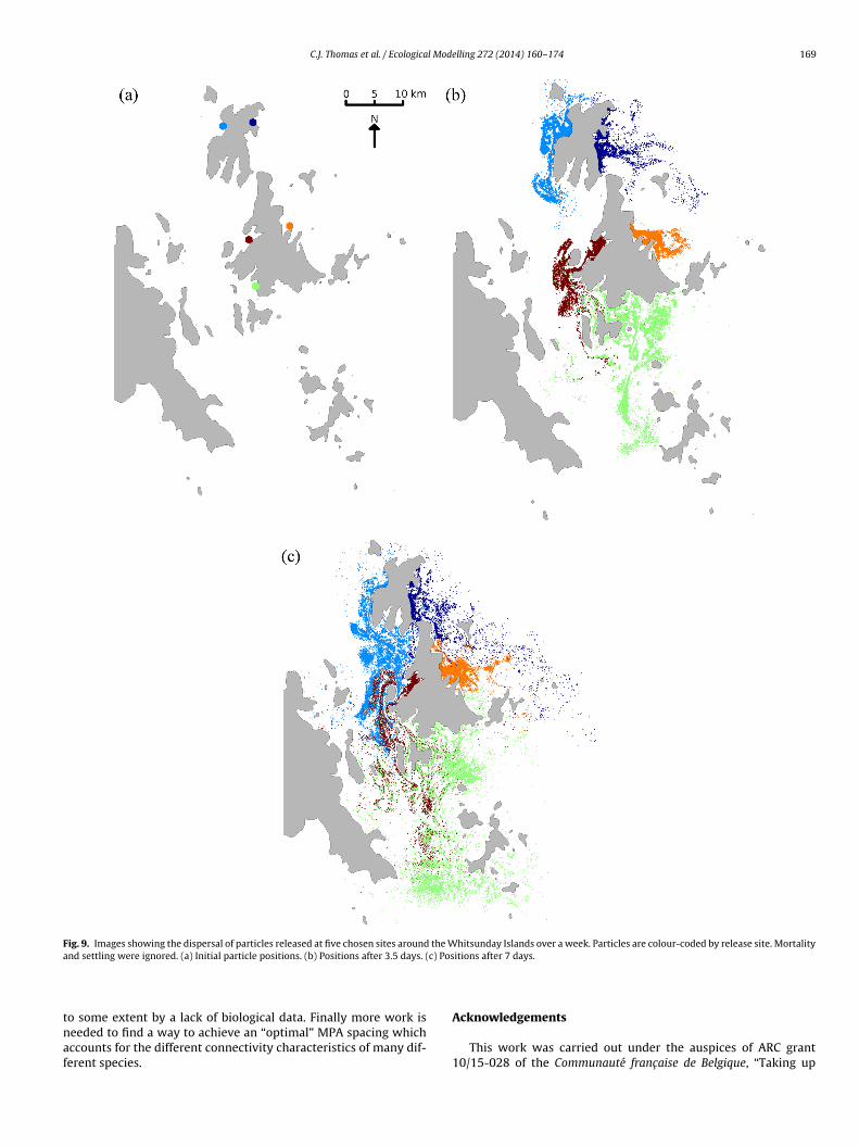
The work carried out by Lambrechts et al. (2008) shows thatthe hydrodynamic model used is able to reproduce small-scale cir-culation features well, however, it is also necessary to validatethe model’s ability to realistically reproduce large-scale circula-tion through the region. This was done by comparing predictionsof sea surface elevation (SSE) and water currents with observeddata at various mooring sites. Data from long-term mooringsobtained from the Integrated Marine Observing System’s (IMOS)Great Barrier Reef Ocean Observing System (GBROOS) program runby AIMS/CSIRO were used to validate SSE, whilst current meterdata from a variety of sources were used to validate water currents.The locations of the mooring points used are shown in Fig. 1. TheSSE observed at different GBROOS mooring sites is shown along-side model predictions for a typical weekly period in Fig. 11. Thereis a good agreement between the two datasets both in terms ofamplitude and phase.

Table 2 shows average longshore current velocities for the dif-

ferent mooring sites compared with model predictions. It shouldbe considered that comparing currents at a given point is very del-icate, as any discrepancy in spatial position and water depth canlead to a relatively large change in the observed current, especially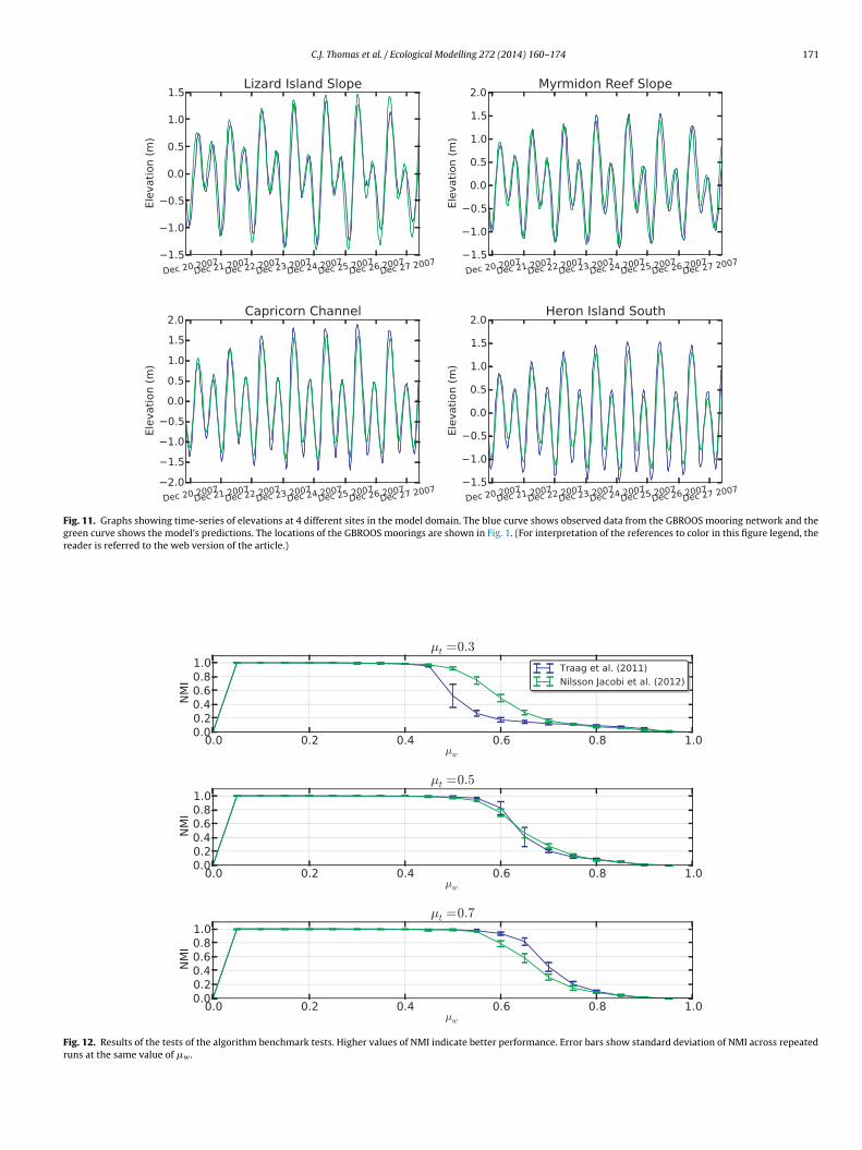

Page 12

C.J. Thomas et al. / Ecological Modelling 272 (2014) 160– 174 171

Fig. 11. Graphs showing time-series of elevations at 4 different sites in the model domain. The blue curve shows observed data from the GBROOS mooring network and thegreen curve shows the model’s predictions. The locations of the GBROOS moorings are shown in Fig. 1. (For interpretation of the references to color in this figure legend, thereader is referred to the web version of the article.)

Fig. 12. Results of the tests of the algorithm benchmark tests. Higher values of NMI indicate better performance. Error bars show standard deviation of NMI across repeatedruns at the same value of w .

Page 13

172 C.J. Thomas et al. / Ecological Modelling 272 (2014) 160– 174

Table 2Observed longshore residual currents (UO) and simulated longshore residual currents (USLIM), in m s−1 at various sites in the GBR. Positive indicates a northerly longshoredirection, whereas negative indicates a southerly longshore direction. The Source column gives the source of UO . Locations of moorings shown in Fig. 1. Sources: A: Brinkmanet al. (2001), B: Andutta et al. (2012), C: Wolanski et al. (1989), D: Middleton and Cunningham (1984)

Site Latitude (◦ S) Longitude (◦ E) USLIM UO Source

Lizard Island 14.7406 145.4253 0.05 0.05 ACape Upstart 19.6253 147.9142 −0.04 −0.11 AOld Reef 19.4071 148.0197 −0.14 −0.10 BBowden Reef 19.0600 147.9597 0.00 −0.02 CRattray Island 19.9826 148.5833 −0.03 −0.08 B

cttgdtd

Aa

awtwscG

B

LWsppuamdtwaqmtscd

TCto

though the method of Nilsson Jacobi et al. (2012) worked better fornetworks with lower values of t, whilst the method of Traag et al.(2011) worked marginally better for networks with higher valuesof t.

Hook 19.9400 149.1100Bushy 20.8900 150.1600

Bell 21.8200 151.1400

lose to reefs and islands – which is where most observing sta-ions are situated – as the horizontal shear is often significant inhese areas. In this context, Table 2 shows that there is a relativelyood agreement between the model predictions and the observedataset. We can therefore be relatively confident in the ability ofhe ocean model to realistically reproduce currents and SSE in theomain.

ppendix B. Comparison of two CPM community detectionlgorithms

We compared the performance of the community detectionlgorithm employed in this study (described in Traag et al., 2011)ith the one used by Nilsson Jacobi et al. (2012), in order to test

he validity of using either approach. We used two methods: firste compared the performance of each algorithm in partitioning a

tandard benchmark network with a known solution, and then weompared the partitions generated by each method for an actualBR connectivity network.

.1. Benchmark networks

The standard benchmark networks used were those described inancichinetti et al. (2008) and Lancichinetti and Fortunato (2009).

e generated directed, weighted benchmark networks and mea-ured the performance of both algorithms in identifying the correctartitions for a range of values of weight and topology mixingarameters (w and t, respectively). The resolution parametersed to partition each network (labelled as � in Traag et al., 2011nd 1/ˇ in Nilsson Jacobi et al., 2012) was calculated as the geo-etric mean of pin and pout, i.e.

√pinpout, using the notation and

efinitions from Lancichinetti and Fortunato (2009), and followinghe same approach as Traag et al. (2011). Ten different networksere generated for each combination of w and t, and the two

lgorithms were in turn applied to partition each network. Theuality of these partitions was measured by calculating the nor-alised mutual information (NMI) between these partitions and

he true partitions for the network. NMI provides a measure of howimilar two sets of partitions are. An average value of NMI was cal-ulated for each combination of w and t, along with its standardeviation.

able 3omparison of Traag et al. (2011) and Nilsson Jacobi et al. (2012) community detec-ion methods for G. retiformis connectivity networks at low, medium and high valuesf � . Each algorithm was run 10 times and average values are shown.

� NMI Number of communities

Traag et al. (2011) Nilsson Jacobi et al. (2012)

0.0004 0.90 44 420.00003 0.79 17 150.000006 0.87 11 9

−0.14 −0.15 D−0.11 −0.13 D−0.04 −0.06 D

The results of the comparison are shown in Fig. 12, where thex-axis spans a range of values of w , and the y-axis shows NMI. Thehigher the NMI, the better the quality of the partitions found by thealgorithm. These results show that both methods performed well,

Fig. 13. Partitioning configurations generated for low-� G. retiformis networkobtained using different community detection algorithms. (a) Method of Traag et al.(2011). (b) Method of Nilsson Jacobi et al. (2012).

Page 14

l Mode

B

tTmtwdanFetu

R

A

A

A

B

B

B

B

C

C

C

d

d

D

D

E

F

F

F

FG

G

G

G

C.J. Thomas et al. / Ecologica

.2. GBR network

Both community detection methods were then used to parti-ion the set of GBR connectivity networks discussed in Section 3.2.able 3 shows the number of communities identified by eachethod for each network, as well as the NMI between the two par-

itions. These indicate that the high- and low-� networks matchell, whilst the middle-� network has a slightly lower NMI. Theifferences between the partitions created by the two algorithmsre generally limited to reefs close to the boundaries of commu-ities being placed in one or the other neighbouring community.ig. 13 compares typical partitioning configurations generated byach algorithm for the low-� case. Overall, the communities iden-ified were not very sensitive to the community detection methodsed.

eferences

lmany, G.R., Connolly, S.R., Heath, D.D., Hogan, J.D., Jones, G.P., McCook, L.J., Mills,M., Pressey, R.L., Williamson, D.H., 2009. Connectivity, biodiversity conserva-tion and the design of marine reserve networks for coral reefs. Coral Reefs 28,339–351.

ndutta, F.P., Ridd, P.V., Wolanski, E., 2011. Dynamics of hypersaline coastal watersin the Great Barrier Reef. Estuarine, Coastal and Shelf Science 94, 299–305.

ndutta, F.P., Kingsford, M.J., Wolanski, E., 2012. ‘Sticky water’ enables the retentionof larvae in a reef mosaic. Estuarine, Coastal and Shelf Science 54, 655–668.

eaman, R.J., 2010. Project 3DGBR: A High-Resolution Depth Model for the Great Bar-rier Reef and Coral Sea. Final Report Project 2.5i.1a, Marine and Tropical SciencesResearch Facility (MTSRF), Cairns, Australia.

londel, V.D., Guillaume, J-.L., Lambiotte, R., Lefebvre, E., 2008. Fast unfolding ofcommunities in large networks. Journal of Statistical Mechanics: Thoery andExperiment 10, P10008.

rinkman, R., Wolanski, E., Deleersnijder, E., McAllister, F., Skirving, W., 2001.Oceanic inflow from the Coral Sea into the Great Barrier Reef. Estuarine, Coastaland Shelf Science 54, 655–668.

uston, P.M., Jones, G.P., Planes, S., Thorrold, S.R., 2012. Probability of successfullarval dispersal declines fivefold over 1 km in a coral reef fish. Proceedings ofthe Royal Society B 279, 1883–1888.

onnolly, S.H., Baird, A.R., 2010. Estimating dispersal potential for marine larvae:dynamic models applied to scleractinian corals. Ecology 91 (12), 3572–3583.

owen, R.K., Sponaugle, S., 2009. Larval dispersal and marine population connectiv-ity. Annual Review of Marine Science 1, 443–466.

owen, R.K., Paris, C.B., Srinivasan, A., 2006. Scaling of connectivity in marine popu-lations. Science 311, 522–527.

e Brauwere, A., de Brye, B., Blaise, S., Deleersnijder, E., 2011. Residence time, expo-sure time and connectivity in the Scheldt estuary. Journal of Marine Systems 84(3/4), 85–95.

e Brye, Benjamin, Anouk de Brauwere, Olivier Gourgue, Tuomas Karna, JonathanLambrechts, Richard Comblen, Eric Deleersnijder, 2010. A finiteelement: multi-scale model of the scheldt tributaries, river, estuary and rofi. Coastal Engineering57 (9), 850–863.

eleersnijder, E., Norro, A., Wolanski, E., 1992. A three-dimensional model of thewater circulation around an island in shallow water. Continental Shelf Research12 (7/8), 891–906.

rew, J.A., Barber, P.H., 2012. Comparative phylogeography in Fijian coral reef fishes:a multi-taxa approach towards marine reserve design. PLoS ONE 7 (10).

gbert, G.D., Erofeeva, S.Y., 2002. Efficient inverse modeling of barotropic oceantides. Journal of Atmospheric and Oceanic Technology 19, 183–204.

alconer, R., Wolanski, E., Mardapitta-Hadjipandeli, L., 1986. Modeling tidal cir-culation in an island’s wake. Journal of Waterway, Port, Coastal, and OceanEngineering 112, 234–254.

isher, R., Bellwood, D.R., 2003. Undisturbed swimming behaviour and nocturnalactivity of coral reef fish larvae. Marine Ecology Progress Series 263, 177–188.

ortunato, S., 2007. Resolution limit in Community Detection. Proceedings of theNational Academy of Sciences 104, 36–41.

ortunato, S., 2010. Community detection in graphs. Physics Reports 486, 75–174.BRMPA, 2007. Coastal Features within and Adjacent to the Great Barrier Reef

World Heritage Area. Technical report, Great Barrier Reef Marine Park Authority,Australia.

erlach, G., Atema, J., Kingsford, M.J., Black, K.P., Miller-Sims, V., 2007. Smelling homecan prevent dispersal of reef fish larvae. Proceedings of the National Academyof Sciences of the United States of America 104 (3), 858–863.

rimm, V., Berger, U., Bastiansen, F., Eliassen, S., Ginot, V., Giske, J., Goss-Custard, J.,Grand, T., Heinz, S.K., Huse, G., Huth, A., Jepsen, J.U., Jorgensen, C., Mooij, W.M.,Muller, B., Pe’er, G., Piou, C., Railsback, S.F., Robbins, A.M., Robbins, M.M., Ross-

manith, E., Ruger, N., Strand, E., Souissi, S., Stillman, R.A., Vabo, R., Visser, U.,DeAngelis, D.L., 2006. A standard protocol for describing individual-based andagent-based models. Ecological Modelling 198, 115–126.

uizien, K., Belharet, M., Marsaleix, P., Guarinia, J.M., 2012. Using larval dis-persal simulations for marine protected area design. Application to the Gulf

lling 272 (2014) 160– 174 173

of Lions (northwest Mediterranean). Limnology and Oceanography 57 (4),1099–1112.

Hamann, M., Grech, A., Wolanski, E., Lambrechts, J., 2011. Modelling the fate ofmarine turtle hatchlings. Ecological Modelling 222, 1515–1521.

Hunter, J.R., Craig, P.D., Phillips, H.E., 1993. On the use of random waml mod-els with spatially variable diffusivity. Journal of Computational Physics 106,366–376.

Jones, G.P., Almany, G.R., Russ, G.R., Sale, P.F., Steneck, R.S., van Oppen, M.J.H.,Willis, B.L., 2009. Larval retention and connectivity among populations ofcorals and reef fishes: history and advances and challenges. Coral Reefs 28,307–323.

Kalnay, E., Kanamitsu, M., Kistler, R., Collins, W., Deaven, D., Gandin, L., Iredell, M.,Saha, S., White, G., Woollen, J., Zhu, Y., Leetmaa, A., Reynolds, B., Chelliah, M.,Ebisuzaki, W., Higgins, W., Janowiak, J., Mo, K.C., Ropelewski, C., Wang, J., Jenne,R., Joseph, D., 1996. The ncep/ncar 40-year reanalysis project. Bulletin of theAmerican Meteorological Society 77, 437–470.

Kininmonth, S., van Oppen, M.J.H., Possingham, H.P., 2010a. Determining the com-munity structure of the coral Seriatopora hystrix from hydrodynamic andgenetic networks. Ecological Modelling 221, 2870–2880.

Kininmonth, S.J., De’ath, G., Possingham, H.P., 2010b. Graph theoretic topology ofthe Great but small Barrier Reef world. Theoretical Ecology 3, 75–88.

Lambrechts, J., Hanert, E., Deleersnijder, E., Bernard, P.-E., Legat, V., Remacle, J.-F.,Wolanski, E., 2008. A multi-scale model of the hydrodynamics of the wholeGreat Barrier Reef. Estuarine, Coastal and Shelf Science 79, 143–151.

Lancichinetti, A., Fortunato, S., 2009. Community detection algorithms: A compara-tive analysis. Physical Review E 80, 056117.

Lancichinetti, A., Fortunato, S., Radicchi, F., 2008. Benchmark graphs for testing com-munity detection algorithms. Physical Review E 78, 46110.

Largier, J.L., 2003. Considerations in estimating larval dispersal distances fromoceanographic data. Ecological Applications 13, S71–S89.

Legrand, S., Deleersnijder, E., Hanert, E., Legat, V., Wolanski, E., Highresolution,2006. unstructured meshes for hydrodynamic models of the Great Barrier Reef,Australia. Estuarine, Coastal and Shelf Science 68, 36–46.

Leis, J.M., Van Herwerden, L., Patterson, H.M., 2011. Estimating connectivity inmarine fish populations: what works best. Oceanography and Marine Biology:An Annual Review 49, 193–234.

Luick, J.L., Mason, L., Hardy, T., Furnas, M.J., 2007. Circulation in the Great BarrierReef lagoon using numerical tracers and in situ data. Continental Shelf Research27, 757–778.

Middleton, J.H., Cunningham, A., 1984. Wind-forced continental shelf waves from ageographical origin. Continental Shelf Research 3 (3), 215–232.

Mumby, P.J., Elliott, I.A., Eakin, M., Skirving, W., Paris, C.B., Edwards, H.J., Enriquez, S.,Iglesias-Prieto, R., Cherubin, L.M., Stevens, J.R., 2011. Reserve design for uncer-tain responses of coral reefs to climate change. Ecology Letters 14, 132–140.

Munday, P.L., Leis, J.M., Lough, J.M., Paris, C.B., Kingsford, M.J., Berumen, M.L., Lam-brechts, J., 2009. Climate change and coral reef connectivity. Coral Reefs 28,379–395.

Newman, M.E.J., Girvan, M., 2004. Finding and evaluating community structure innetworks. Physical Review E 69, 026113.

Nilsson Jacobi, M., Andre, C., Doos, K., Jonsson, P.R., 2012. Identification of subpop-ulations from connectivity matrices. Physical Review E 69, 026113.

Okubo, A., 1971. Oceanic diffusion diagrams. Deep Sea Research 18, 789–802.Olds, A.D., Connolly, R.M., Pitt, K.A., Maxwell, P.S., 2012. Habitat connectivity

improves reserve performance. Conservation Letters 5, 56–63.Palumbi, S.R., 2003. Population genetics and demographic connectivity and and the

design of marine reserves. Ecological Applications 13, S146–S158.Paris, C.B., Cherubin, L.M., Cowen, R.K., 2007. Surfing and spinning and or diving from

reef to reef: effects on population connectivity. Marine Ecology Progress Series347, 285–300.

Proulx, S.R., Promislow, D.E.L., Phillips, P.C., 2005. Network thinking in ecology andevolution. Trends in Ecology and Evolution 20 (6), 345–353.

Ronhovde, P., Nussinov, Z., 2010. Local resolution-limit-free Potts model for com-munity detection. Physical Review E 81, 046114.

Sassi, M.G., Hoitink, A.J.F., De Brye, B., Vermeulen, B., Deleersnijder, E., 2011. Tidalimpact on the division of river discharge over distributary channels in theMahakam Delta. Ocean Dynamics 61, 2211–2228.

Smith, S.D., Banke, E.G., 1975. Variation of the sea surface drag coefficient with windspeed. Quarterly Journal of the Royal Meteorological Society 101, 665–673.

Spagnol, S., Wolanski, E., Deleersnijder, E., Brinkman, R., McAllister, F., Cushman-Roisin, B., Hanert, E., 2001. An error frequently made in the evaluationof advective transport in two-dimensional Lagrangian models of advection-diffusion in coral reef waters. Marine Ecology Progress Series 235,299–302.

Traag, V.A., Van Dooren, P., Nesterov, Y., 2011. Narrow scope for resolution limit-freecommunity detection. Physical Review E 84, 016114.

Treml, E., Halpin, P., Urban, D., Pratson, L., 2008. Modeling population connectivity byocean currents, a graph-theoretic approach for marine conservation. LandscapeEcology 23, 19–36.

Vermeij, M.J.A., Marhaver, K.L., Huijbers, C.M., Nagelkerken, I., Simpson, S.D., 2010.Coral larvae move toward reef sounds. PLoS ONE 5 (5).

Werner, F., Cowen, R., Paris, C.B., 2007. Coupled biological and physical models:

present capabilities and necessary developments for future studies of popula-tion connectivity. Oceanography 20, 54–69.

White, L., Deleersnijder, E., 2007. Diagnoses of vertical transport in a three-dimensional finite element model of the tidal circulation around an island.Estuarine, Coastal and Shelf Science 74, 655–669.

Page 15

1 l Mod

W

W

W

74 C.J. Thomas et al. / Ecologica

olanski, E., 1994. Physical Oceanographic Processes of the Great Barrier Reef. CRCPress, Boca Raton, FL.

olanski, E., Spagnol, S., 2000. Sticky waters in the Great Barrier Reef. Estuarine,Coastal and Shelf Science 50, 27–32.

olanski, E., Burrage, D., King, B., 1989. Trapping and diffusion of coral eggs nearBowden Reef, Great Barrier Reef following mass coral spawning. ContinentalShelf Research 9, 479–496.

elling 272 (2014) 160– 174

Wolanski, E., Brinkman, R., Spagnol, S., McAllister, F., Steinberg, C., Skirving, W.,Deleersnijder, E., 2003. Chapter 15 – merging scales in models of water cir-

culation: perspectives from the Great Barrier Reef. In: Lakhan, V.C. (Ed.),Advances in Coastal Modeling, vol. 67 of Elsevier Oceanography Series. Elsevier,pp. 411–429.

Wolanski, E., Lambrechts, J., Thomas, C., Deleersnijder, E., 2013. The net water cir-culation through Torres strait. Continental Shelf Research 64, 66–74.