Numerical modeling of turbulence mixed convection heat transfer in air filled enclosures by finite volume method

Int. Jnl. of Multiphysics Volume 5 · Number 4 · 2011 307

Numerical modeling of turbulence mixedconvection heat transfer in air filled enclosures by

finite volume methodMohammad Reza Safaei1*, Marjan goodarzi1 and

Mohammadali Mohammadi21Mashhad Branch, Islamic Azad University, Mashhad, Iran

2University Putra Malaysia, Serdang, Malaysia

ABSTRACT

In the present study, first the turbulent natural convection and then laminar

mixed convection of air flow was solved in a room and the calculated

outcomes are compared with results of other scientists and after showing

validation of calculations, aforementioned flow is solved as a turbulent

mixed convection flow, using the valid turbulence models Standard k−ε,

RNG k−ε and RSM.

To solve governing differential equations for this flow, finite volume

method was used. This method is a specific case of residual weighting

method. The results show that at high Richardson Numbers, the flow is

rather stationary at the center of the enclosure. Moreover, it is distinguished

that when Richardson Number increases the maximum of local Nusselt

decreases. Therefore, it can be said that less number of Richardson

Number, more rate of heat transfer.

Keywords: Mixed Convection Heat Transfer, Turbulence Models, Nusselt

Number, Turbulent Kinetic Energy, Reynolds Stress.

1. INTRODUCTIONMixed convection heat transfer is a phenomenon in which both natural and forcedconvections happen. Mixed convection heat transfer takes place either when buoyancy effectmatters in a forced flow or when there are sizable effects of forced flow in a buoyancy flow.Dimensionless numbers to determine this type of flow are as follows: Grashof Number(Gr = g.β.∆T.L3/v2), Reynolds Number (Re = ρ.v.l/µ), Rayleigh Number (Ra = Gr.Pr),Prandtl Number (Pr = Cp.µ/K), and Richardson Number (Ri). If you devide naturalconvection effect by forced convection effect, it yields to Richardson number and it is writtenas such: Ri = Gr/Re2. When it comes to limits and we have Ri→0 or Ri→∞, forcedconvection and natural convection become dominant heat transfers respectively [Bejan [1]].

Mixed convection heat transfer is a fundamentally significant heat transfer mechanismthat occurs in selection industrial and technological applications.

In the recent years, wide and practical usages of mixed convection heat transfer in areassuch as designing solar collectors, double-layer glasses, building insulations, coolingelectronic parts and have attracted many scientists in studying it.

*Corresponding author. Tel.: +989151022063; E-mail address: [email protected]

308 Numerical modeling of turbulence mixed convection heat transfer in air filledenclosures by finite volume method

Fluid flow and heat transfer in rectangular or square cavities driven have been studiedextensively in the literature. A review shows that there are two kinds of studies:

One way includes the entry of hot (or cold) fluid from one side, passing isothermal walls,and exit from the other side. In this case, we could evaluate and compare the forcedconvection effect caused by the entry and exit of the fluid. Some scientists have appliedthermal flux on the way fluid passes through the channel and then, they studied the effectsof it. Among the studies, we can mention the ones done by Rahman et al. [2], Saha et al. [3]and Saha et al. [4]. Another method to create mixed convections is to move enclosure wallsin presence of hot (cold) fluid inside the enclosure. This creates shear stresses and providesthermal and hydrodynamic boundary layers in the fluid inside the enclosure, and eventuallycreates forced convection in it. Numerous studies have been conducted in this field so far.We can mention the study done by Ghasemi & Aminossadati [5] as an instance. They havestudied heat transfer of natural convection in an inclined square enclosure that had twoinsulated vertical walls and two horizontal walls with different temperatures with using finitevolume method. They studied pure water and CuO-water with 0.01 ≤ Φ ≤ 0.04. They variedRayleigh number between 103 and 107 and inclination angle between 0 Degrees to 90Degrees and studied the impact of these factors on heat transfer and fluid flow in theenclosure. They found that in low Rayleigh numbers - which heat transfer, is in a conductionway — flow pattern and temperature in the inclination angles range of 30 degrees to 90degrees is similar. However, for Rayleigh numbers bigger than 105, temperature and flowpattern is different in inclination angle = 0 degree from other inclination angles.

Basak et al. [6] Studied the mixed convection flow inside a square enclosure with left andright cold walls, insulated moving upper wall, and fixed lower hot wall by using finite elementmethod. They suggested that by increasing Gr, when Pr and Re are fixed, recirculation powerwould improve.

In year 2007, Khanafer et al. [7] numerically studied unsteady mixed convection of asimple fluid in a sinusoidal lid-sliding cavity. Their study showed that Grashof and Reynoldsnumbers had an undeniable impact on nature and structure of the flow.

It is undeniable that the advancement in different sciences in the last decade has resultedin much subtle laboratory measuring tools and it is true that using of modern methods likeparallel processing has enabled us to efficiently use numerical analysis methods. Yet analysisof turbulent flows inside the enclosure is still a challenging topic in fluid mechanics. That isbecause in experimental situation, it is too difficult to reach ideal adiabatic wall condition. Itis at the same time difficult to measure low speeds in enclosure boundary layers throughusing present sensors and probes. Even numerically, although numerical methods like DES,LES, and DNS have been subject to dramatic advancements, it is still nearly impossible topredict the stratification in the core of the enclosure. Non-linearity and coupling of thepredominant equations have contributed into making the calculations complicated and timeconsuming. That is while in designing large enclosures, Rayleigh number is usually large,and so the flow nature is turbulent [Goshayeshi and safaei [8]]. The complexity ofcalculations in mixed convection has made scientists to just study natural convection, amongwhich we can mention the studies Bessaih and Kadja [9], Ampofo [10], Salat et al. [11],Xaman et al. [12] and Aounallah et al. [13]. In 2000, Tian and Karayiannis [14] started anexperimental study in South Bank University that was followed by Ampofo and Karayiannis[15]. Data in this work were experimental benchmark data of natural convection flow insidea square enclosure, and were used for other studies. Whereas Peng and Davidson [16] studiedthe mentioned flow by using LES, and Omri and Galanis [17] used the SST k-ω to study thisflow. Hsieh and Lien [18] used turbulence models of steady RANS like Low-Re k-ε, and

numerically analyzed the works done by Betts and Bokhari [19] and Tian and Karayiannis[14]. In the present work, turbulent natural convection inside square and rectangularenclosures is modeled first, and the results have been compared with the studies Betts andBokhari [19] and Tian and Karayiannis [14], Ampofo and Karayiannis [15], Peng andDavidson [16], Omri and Galanis [17] and Hsieh and Lien [18]. After the calculations beingvalid, first the Laminar mixed convection flow is solved in the square enclosure, incomparison with Basak et al. [6] and eventually turbulence mixed convection in squareenclosure is modeled for the first time in all of the world, by using turbulence models likeStandard k-ε, RNG k-ε and RSM.

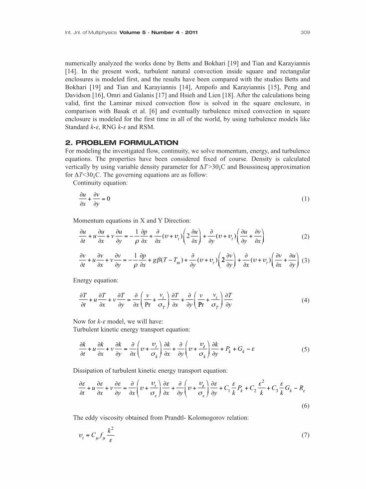
2. PROBLEM FORMULATIONFor modeling the investigated flow, continuity, we solve momentum, energy, and turbulenceequations. The properties have been considered fixed of course. Density is calculatedvertically by using variable density parameter for ∆T >30¡C and Boussinesq approximationfor ∆T<30¡C. The governing equations are as follow:

Continuity equation:

(1)

Momentum equations in X and Y Direction:

(2)

(3)

Energy equation:

(4)

Now for k-ε model, we will have:Turbulent kinetic energy transport equation:

(5)

Dissipation of turbulent kinetic energy transport equation:

(6)

The eddy viscosity obtained from Prandtl- Kolomogorov relation:

(7)υεµ µt C fk

=2

∂∂

+∂∂

+∂∂

=∂∂

+

∂∂

+∂∂

+ε ε ε

υυ

σε

υυ

εtu

xv

y x x yt tt

k kyC

kP C

kC

kG R

σε ε ε ε

εε

∂∂

+ + + −1 2

2

3

∂∂

+∂∂

+∂∂

=∂∂

+

∂∂

+∂∂

+k

tu

k

xv

k

y x

k

x yt

k

υυ

συ

υtt

kk k

k

yP G

σε

∂∂

+ + −

∂∂

+∂∂

+∂∂

=∂∂

+

∂∂

+∂∂

T

tu

T

xv

T

y x

v v T

x y

vt

TPr σ PPr+

∂∂

v T

yt

Tσ

∂∂

+∂∂

+∂∂

= −∂∂

+ − +∂∂

+v

tu

v

xv

v

y

p

xg T T

ym t

1ρ

β υ υ( ) ( ) 22∂∂

+

∂∂

+∂∂

+∂∂

v

y x

v

x

u

yt( )υ υ

∂∂

+∂∂

+∂∂

= −∂∂

+∂∂

+∂∂

u

tu

u

xv

u

y

p

x x

u

xt

12

ρυ υ( )

+

∂∂

+∂∂

+∂∂

y

u

y

v

xt( )υ υ

∂∂

+∂∂

=u

x

v

y0


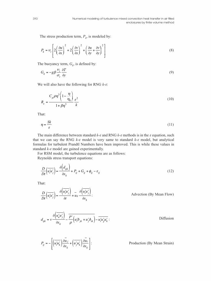
The stress production term, Pk, is modeled by:

(8)

The buoyancy term, Gk, is defined by:

(9)

We will also have the following for RNG k-ε:

(10)

That:

(11)

The main difference between standard k-ε and RNG k-ε methods is in the ε equation, suchthat we can say the RNG k-ε model is very same to standard k-ε model, but analyticalformulas for turbulent Prandtl Numbers have been improved. This is while these values instandard k-ε model are gained experimentally.

For RSM model, the turbulence equations are as follows:Reynolds stress transport equations:

(12)

That:

Advection (By Mean Flow)

Diffusion

Production (By Mean Strain)P u uu

xu u

u

xij i kj

kj k

i

k

= − ′ ′( ) ∂∂ + ′ ′( ) ∂∂

:

d vu u

x

Pu u u uijk

u j

ki jk j ik i=

∂ ′ ′( )∂

−′

′ + ′( )− ′ ′ρ

δ δ jj ku′ :

D

Dtu u

u u

tu

u u

xi j

i jk

i j

k

′ ′( ) =∂ ′ ′( )

∂+

∂ ′ ′( )∂

:

D

Dtu u

d

xP Gi j

ijk

kij ij ij ij′ ′( ) =

∂( )∂

+ + + −φ ε

ηε

=Sk

R

C

kε

µρηηη

βη

ε=

−

+

3

03

21

1

G gT

ykt

t

= −∂∂

βυ

σ

Pu

x

v

x

u

y

v

yk t=∂∂

+

∂∂

+

∂∂

+∂∂

υ 2 2

2 2

2


Production (By Body Force)

Pressure-Strain Correlation

Dissipation

Turbulent kinetic energy transport equation:

(13)

Except the terms Convection and Production in Reynolds stress transport equation, all theother terms have contributed in introducing a series of correlations, which have to beidentified according to some known and unknown quantities, so that the equation system canbe configured.

Diffusion term:

(14)

Redistribution term:

(15)

That:

(16)

�φε

φijw

i jw

ijCk

u u C= − ′ ′ +1 22( ) ( ) ( )

φ φ δ φ φ ψijw

kl k l ij ik j k jk i kn n n n n n( ) = − −

� � �3

232

φ δij ij kk ijC P P( )22

13

= − −

φε

δij i j ijCk

u u k( )11

23

= − ′ ′ −

φ φ φ φij ij ij ijw= + +( ) ( ) ( )1 2

− ′ ′ ′ = ′ ′∂ ′ ′

∂u u u C

ku u

u u

xi j k S k li j

lε

Dk

Dt

d

xP Gi

k

i

k k=∂

∂+ + −

( )( ) ( ) ε

εiji

k

j

k

vu

x

u

x=

∂ ′

∂

∂ ′

∂2 :

φρ ρij

i

j

j

iij

P u

x

u

x

PS=

′ ∂ ′

∂+∂ ′

∂

=

′2:

G u f u fij i j j i= ′ ′+ ′ ′( ) :


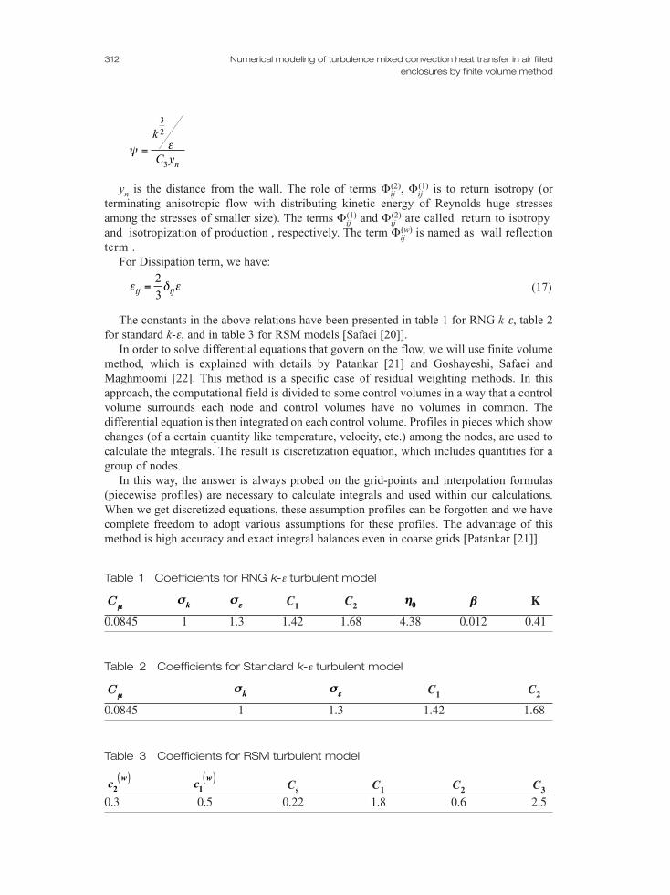
yn is the distance from the wall. The role of terms Φij(2), Φij

(1) is to return isotropy (orterminating anisotropic flow with distributing kinetic energy of Reynolds huge stressesamong the stresses of smaller size). The terms Φij

(1) and Φij(2) are called return to isotropy

and isotropization of production , respectively. The term Φij(w) is named as wall reflection

term .For Dissipation term, we have:

(17)

The constants in the above relations have been presented in table 1 for RNG k-ε, table 2for standard k-ε, and in table 3 for RSM models [Safaei [20]].

In order to solve differential equations that govern on the flow, we will use finite volumemethod, which is explained with details by Patankar [21] and Goshayeshi, Safaei andMaghmoomi [22]. This method is a specific case of residual weighting methods. In thisapproach, the computational field is divided to some control volumes in a way that a controlvolume surrounds each node and control volumes have no volumes in common. Thedifferential equation is then integrated on each control volume. Profiles in pieces which showchanges (of a certain quantity like temperature, velocity, etc.) among the nodes, are used tocalculate the integrals. The result is discretization equation, which includes quantities for agroup of nodes.

In this way, the answer is always probed on the grid-points and interpolation formulas(piecewise profiles) are necessary to calculate integrals and used within our calculations.When we get discretized equations, these assumption profiles can be forgotten and we havecomplete freedom to adopt various assumptions for these profiles. The advantage of thismethod is high accuracy and exact integral balances even in coarse grids [Patankar [21]].

ε δ εij ij=23

ψ ε=k

C yn

32

3


Table 1 Coefficients for RNG k-ε turbulent model

C1 C2 K

0.0845 1 1.3 1.42 1.68 4.38 0.012 0.41

ββηη0σσεεσσkCµµ

Table 2 Coefficients for Standard k-ε turbulent model

C1 C2

0.0845 1 1.3 1.42 1.68

σσεεσσkCµµ

Table 3 Coefficients for RSM turbulent model

Cs C1 C2 C3

0.3 0.5 0.22 1.8 0.6 2.5

cw

1( )c

w2

( )

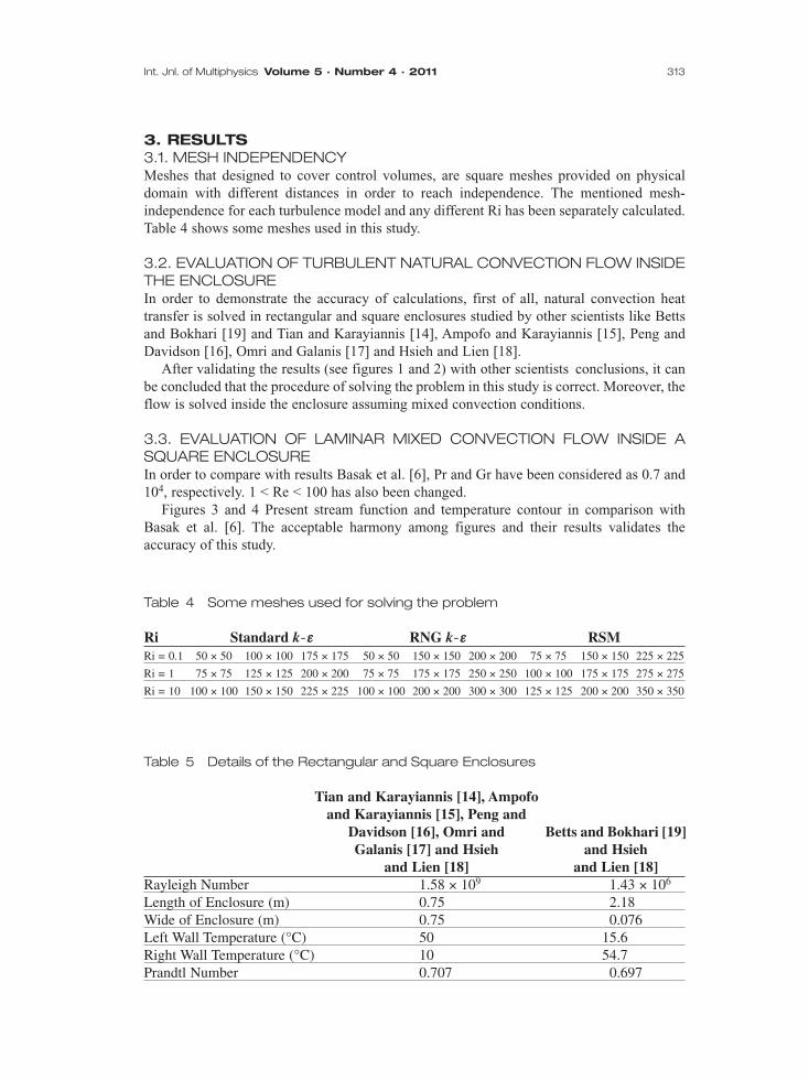
3. RESULTS3.1. MESH INDEPENDENCYMeshes that designed to cover control volumes, are square meshes provided on physicaldomain with different distances in order to reach independence. The mentioned mesh-independence for each turbulence model and any different Ri has been separately calculated.Table 4 shows some meshes used in this study.

3.2. EVALUATION OF TURBULENT NATURAL CONVECTION FLOW INSIDETHE ENCLOSUREIn order to demonstrate the accuracy of calculations, first of all, natural convection heattransfer is solved in rectangular and square enclosures studied by other scientists like Bettsand Bokhari [19] and Tian and Karayiannis [14], Ampofo and Karayiannis [15], Peng andDavidson [16], Omri and Galanis [17] and Hsieh and Lien [18].

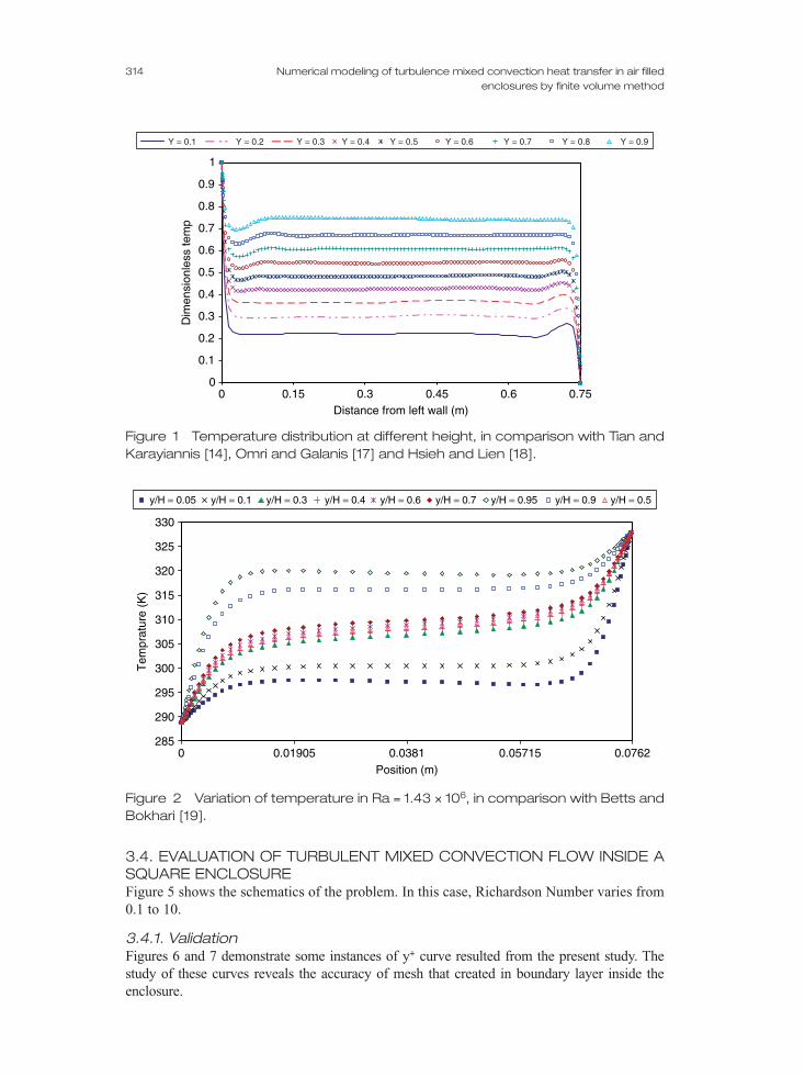
After validating the results (see figures 1 and 2) with other scientists conclusions, it canbe concluded that the procedure of solving the problem in this study is correct. Moreover, theflow is solved inside the enclosure assuming mixed convection conditions.

3.3. EVALUATION OF LAMINAR MIXED CONVECTION FLOW INSIDE ASQUARE ENCLOSUREIn order to compare with results Basak et al. [6], Pr and Gr have been considered as 0.7 and104, respectively. 1 < Re < 100 has also been changed.

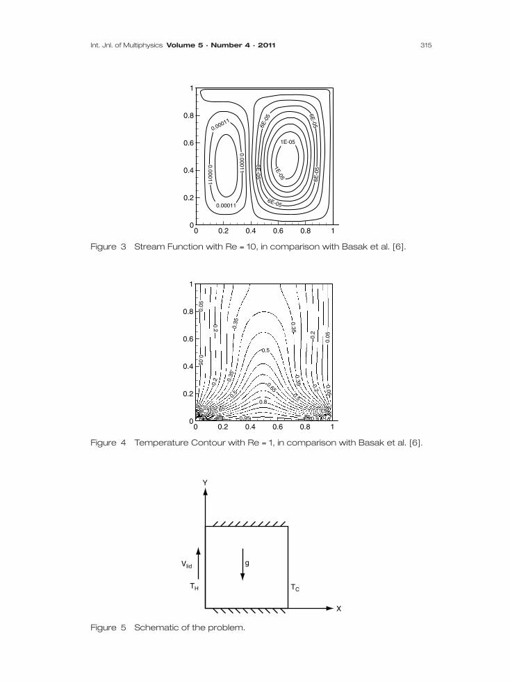
Figures 3 and 4 Present stream function and temperature contour in comparison withBasak et al. [6]. The acceptable harmony among figures and their results validates theaccuracy of this study.


Table 4 Some meshes used for solving the problem

Ri Standard k-ε RNG k-ε RSMRi = 0.1 50 × 50 100 × 100 175 × 175 50 × 50 150 × 150 200 × 200 75 × 75 150 × 150 225 × 225

Ri = 1 75 × 75 125 × 125 200 × 200 75 × 75 175 × 175 250 × 250 100 × 100 175 × 175 275 × 275

Ri = 10 100 × 100 150 × 150 225 × 225 100 × 100 200 × 200 300 × 300 125 × 125 200 × 200 350 × 350

Table 5 Details of the Rectangular and Square Enclosures

Tian and Karayiannis [14], Ampofoand Karayiannis [15], Peng and

Davidson [16], Omri and Betts and Bokhari [19] Galanis [17] and Hsieh and Hsieh

and Lien [18] and Lien [18]Rayleigh Number 1.58 × 109 1.43 × 106

Length of Enclosure (m) 0.75 2.18Wide of Enclosure (m) 0.75 0.076Left Wall Temperature (°C) 50 15.6Right Wall Temperature (°C) 10 54.7Prandtl Number 0.707 0.697

3.4. EVALUATION OF TURBULENT MIXED CONVECTION FLOW INSIDE ASQUARE ENCLOSUREFigure 5 shows the schematics of the problem. In this case, Richardson Number varies from0.1 to 10.

3.4.1. ValidationFigures 6 and 7 demonstrate some instances of y+ curve resulted from the present study. Thestudy of these curves reveals the accuracy of mesh that created in boundary layer inside theenclosure.


0

0.1

0.2

0.3

0.4

0.5

0.6

0.7

0.8

0.9

1

0 0.15 0.3 0.45 0.6 0.75Distance from left wall (m)

Dim

ensi

onle

ss te

mp

Y = 0.1 Y = 0.2 Y = 0.3 Y = 0.4 Y = 0.5 Y = 0.6 Y = 0.7 Y = 0.8 Y = 0.9

Figure 1 Temperature distribution at different height, in comparison with Tian andKarayiannis [14], Omri and Galanis [17] and Hsieh and Lien [18].

285

290

295

300

305

310

315

320

325

330

0 0.01905 0.0381 0.05715 0.0762Position (m)

Tem

prat

ure

(K)

y/H = 0.05 y/H = 0.1 y/H = 0.3 y/H = 0.4 y/H = 0.6 y/H = 0.7 y/H = 0.95 y/H = 0.9 y/H = 0.5

Figure 2 Variation of temperature in Ra = 1.43 × 106, in comparison with Betts andBokhari [19].


0 0.2 0.4 0.6 0.8 1

1

0.8 0.05

0.05

0.2

0.2

0.5

0.5

0.5

0.05

0.65

8

0.65

0.2

0.2

0.05

0.350.35

0.35 0.35

0.8

0.9 0.80.95

0.6

0.4

0.2

0

0 0.2

0.00011

0.00011

6E-05

6E-05

6E-0

5

6E-05

1E-05

1E-05

0.00011

0.00011

0.4 0.6 0.8 1

1

0.8

0.6

0.4

0.2

0

6E-0

5

Figure 3 Stream Function with Re = 10, in comparison with Basak et al. [6].

Figure 4 Temperature Contour with Re = 1, in comparison with Basak et al. [6].

Vlid

TC

g

X

Y

TH

Figure 5 Schematic of the problem.

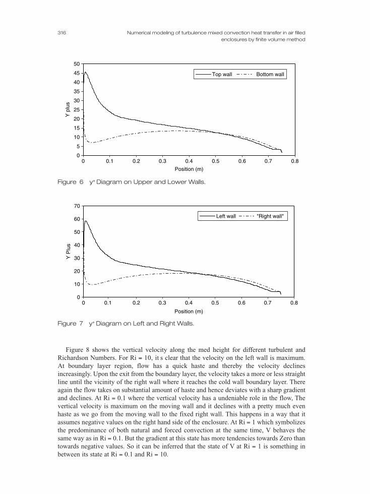
Figure 8 shows the vertical velocity along the med height for different turbulent andRichardson Numbers. For Ri = 10, it s clear that the velocity on the left wall is maximum.At boundary layer region, flow has a quick haste and thereby the velocity declinesincreasingly. Upon the exit from the boundary layer, the velocity takes a more or less straightline until the vicinity of the right wall where it reaches the cold wall boundary layer. Thereagain the flow takes on substantial amount of haste and hence deviates with a sharp gradientand declines. At Ri = 0.1 where the vertical velocity has a undeniable role in the flow, Thevertical velocity is maximum on the moving wall and it declines with a pretty much evenhaste as we go from the moving wall to the fixed right wall. This happens in a way that itassumes negative values on the right hand side of the enclosure. At Ri = 1 which symbolizesthe predominance of both natural and forced convection at the same time, V behaves thesame way as in Ri = 0.1. But the gradient at this state has more tendencies towards Zero thantowards negative values. So it can be inferred that the state of V at Ri = 1 is something inbetween its state at Ri = 0.1 and Ri = 10.


0

5

10

15

20

25

30

35

40

45

50

0 0.1 0.2 0.3 0.4 0.5 0.6 0.7 0.8

Position (m)

Y p

lus

Top wall Bottom wall

Figure 6 y+ Diagram on Upper and Lower Walls.

0

10

20

30

40

50

60

70

0 0.1 0.2 0.3 0.4 0.5 0.6 0.7 0.8

Position (m)

Y P

lus

Left wall "Right wall"

Figure 7 y+ Diagram on Left and Right Walls.

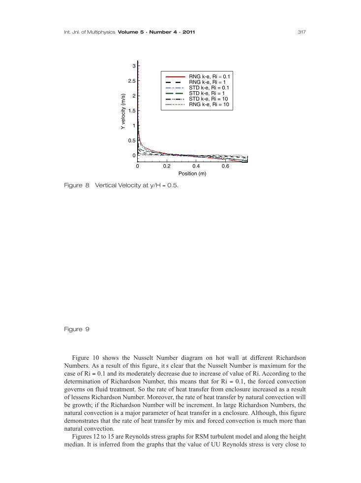
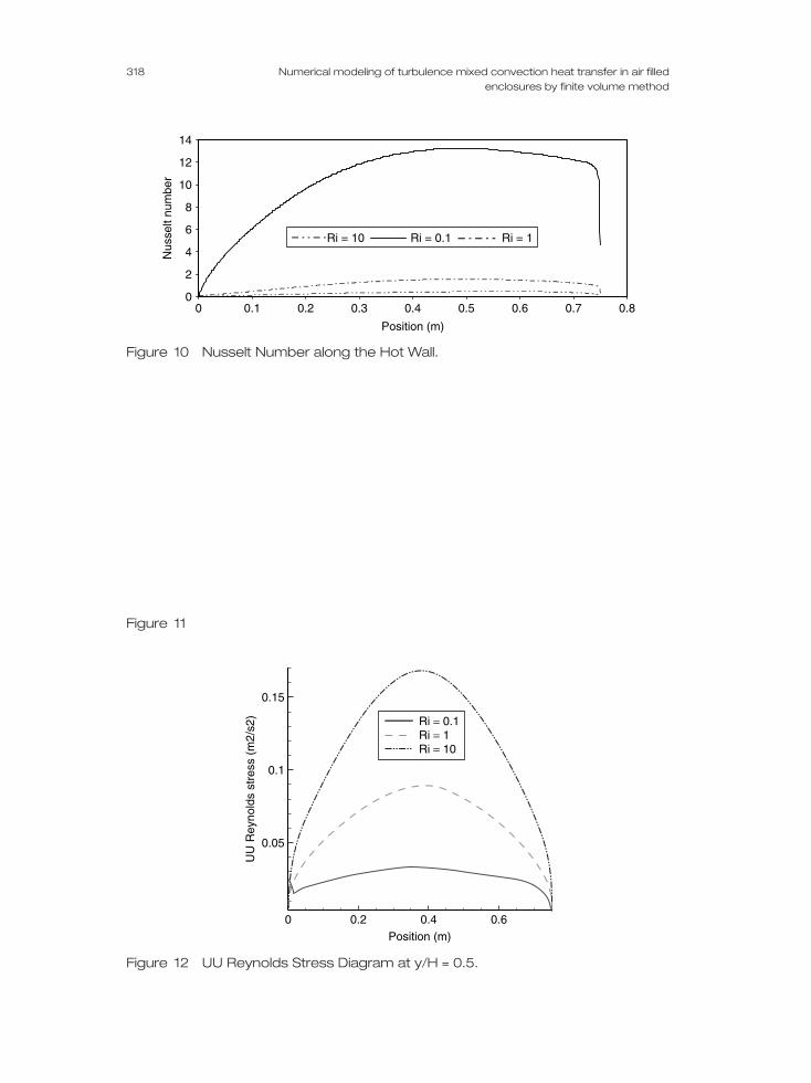
Figure 10 shows the Nusselt Number diagram on hot wall at different RichardsonNumbers. As a result of this figure, it s clear that the Nusselt Number is maximum for thecase of Ri = 0.1 and its moderately decrease due to increase of value of Ri. According to thedetermination of Richardson Number, this means that for Ri = 0.1, the forced convectiongoverns on fluid treatment. So the rate of heat transfer from enclosure increased as a resultof lessens Richardson Number. Moreover, the rate of heat transfer by natural convection willbe growth; if the Richardson Number will be increment. In large Richardson Numbers, thenatural convection is a major parameter of heat transfer in a enclosure. Although, this figuredemonstrates that the rate of heat transfer by mix and forced convection is much more thannatural convection.

Figures 12 to 15 are Reynolds stress graphs for RSM turbulent model and along the heightmedian. It is inferred from the graphs that the value of UU Reynolds stress is very close to


0 0.2 0.4 0.6Position (m)

RNG k-e, Ri = 0.1RNG k-e, Ri = 1STD k-e, Ri = 0.1STD k-e, Ri = 1STD k-e, Ri = 10RNG k-e, Ri = 10

Y v

eloc

ity (

m/s

)

3

2.5

2

1.5

1

0.5

0

Figure 8 Vertical Velocity at y/H = 0.5.

Figure 9


0

2

4

6

8

10

12

14

0 0.1 0.2 0.3 0.4 0.5 0.6 0.7 0.8

Position (m)

Nus

selt

num

ber

Ri = 10 Ri = 0.1 Ri = 1

Figure 10 Nusselt Number along the Hot Wall.

Figure 11

Position (m)0 0.2

0.15

0.1

0.05

UU

Rey

nold

s st

ress

(m

2/s2

)

0.4 0.6

Ri = 0.1Ri = 1Ri = 10

Figure 12 UU Reynolds Stress Diagram at y/H = 0.5.

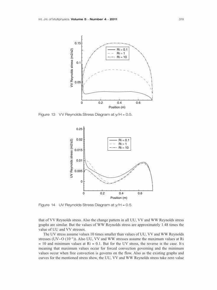
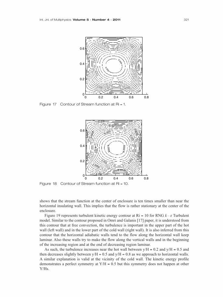
that of VV Reynolds stress. Also the change pattern in all UU, VV and WW Reynolds stressgraphs are similar. But the values of WW Reynolds stress are approximately 1.48 times thevalue of UU and VV stresses.

The UV stress assume values 10 times smaller than values of UU, VV and WW Reynoldsstresses (UV∼O (10−1)). Also UU, VV and WW stresses assume the maximum values at Ri= 10 and minimum values at Ri = 0.1. But for the UV stress, the reverse is the case. It smeaning that maximum values occur for forced convection governing and the minimumvalues occur when free convection is governs on the flow. Also as the existing graphs andcurves for the mentioned stress show, the UU, VV and WW Reynolds stress take zero value


Position (m)0 0.2

0.15

0.1

0.05

VV

Rey

nold

s st

ress

(m

2/s2

)

0.4 0.6

Ri = 0.1Ri = 1Ri = 10

Figure 13 VV Reynolds Stress Diagram at y/H = 0.5.

Position (m)0 0.2

0.25

0.02

0.015

0.01

0.005

0

UV

Rey

nold

s st

ress

(m

2/s2

)

0.4 0.6

Ri = 0.1Ri = 1Ri = 10

Figure 14 UV Reynolds Stress Diagram at y/H = 0.5.

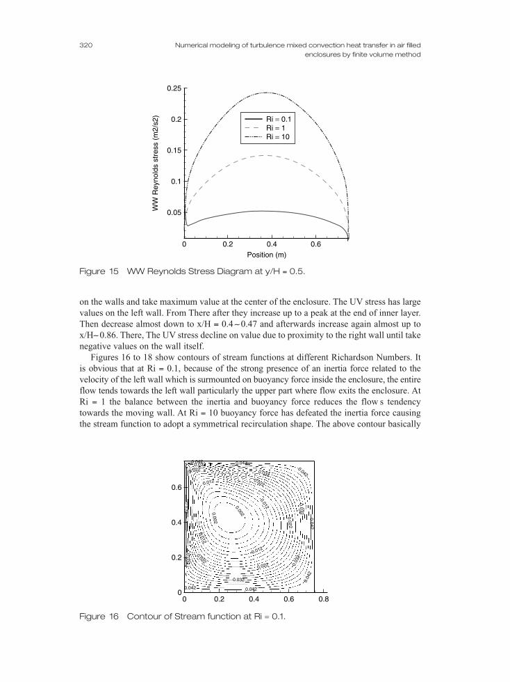
on the walls and take maximum value at the center of the enclosure. The UV stress has largevalues on the left wall. From There after they increase up to a peak at the end of inner layer.Then decrease almost down to x/H = 0.4∼0.47 and afterwards increase again almost up tox/H∼0.86. There, The UV stress decline on value due to proximity to the right wall until takenegative values on the wall itself.

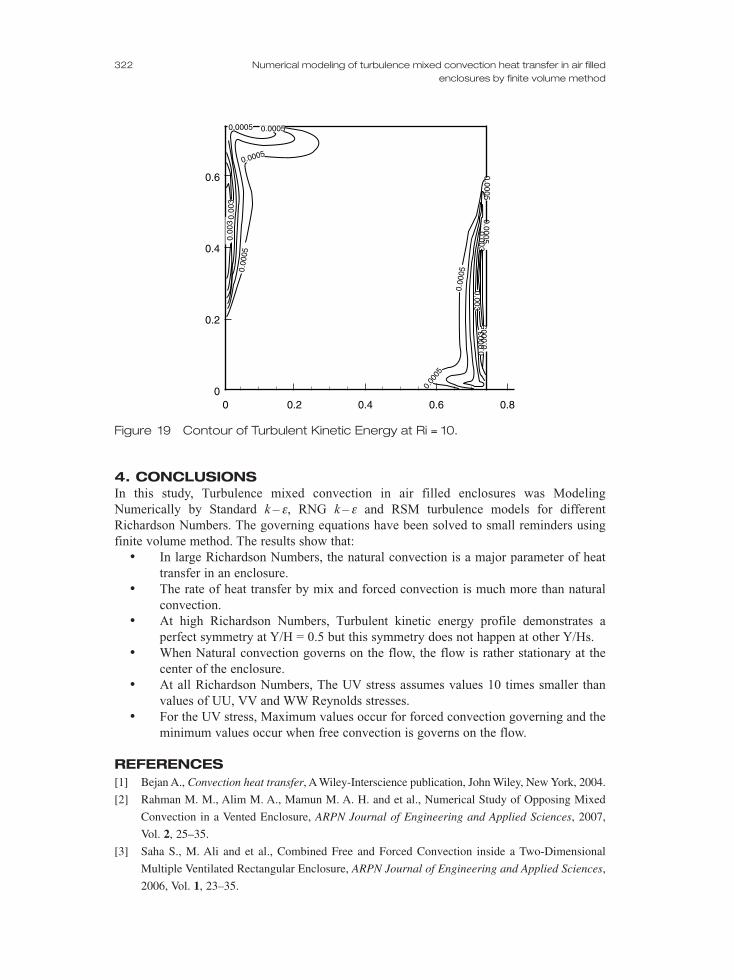
Figures 16 to 18 show contours of stream functions at different Richardson Numbers. Itis obvious that at Ri = 0.1, because of the strong presence of an inertia force related to thevelocity of the left wall which is surmounted on buoyancy force inside the enclosure, the entireflow tends towards the left wall particularly the upper part where flow exits the enclosure. AtRi = 1 the balance between the inertia and buoyancy force reduces the flow s tendencytowards the moving wall. At Ri = 10 buoyancy force has defeated the inertia force causingthe stream function to adopt a symmetrical recirculation shape. The above contour basically


Position (m)0 0.2

0.25

0.2

0.15

0.1

0.05WW

Rey

nold

s st

ress

(m

2/s2

)

0.4 0.6

Ri = 0.1Ri = 1Ri = 10

Figure 15 WW Reynolds Stress Diagram at y/H = 0.5.

0.6

0.0020.002

0.012

0.012

0.012

0.012

0.022

0.022

0.022

0.022

0.022 0.032

0.032

0.032

0.032

0.03

2

0.032

0.032

0.042

0.0420.042

0.042

0.04

2

0.0420.042

0.4

0.2

00 0.2 0.4 0.6 0.8

Figure 16 Contour of Stream function at Ri = 0.1.

shows that the stream function at the center of enclosure is ten times smaller than near thehorizontal insulating wall. This implies that the flow is rather stationary at the center of theenclosure.

Figure 19 represents turbulent kinetic energy contour at Ri = 10 for RNG k−ε Turbulentmodel. Similar to the contour proposed in Omri and Galanis [17] paper, it is understood fromthis contour that at free convection, the turbulence is important in the upper part of the hotwall (left wall) and in the lower part of the cold wall (right wall). It is also inferred from thiscontour that the horizontal adiabatic walls tend to the flow along the horizontal wall keeplaminar. Also these walls try to make the flow along the vertical walls and in the beginningof the increasing region and at the end of decreasing region laminar.

As such, the turbulence increases near the hot wall between y/H = 0.2 and y/H = 0.5 andthen decreases slightly between y/H = 0.5 and y/H = 0.8 as we approach to horizontal walls.A similar explanation is valid at the vicinity of the cold wall. The kinetic energy profiledemonstrates a perfect symmetry at Y/H = 0.5 but this symmetry does not happen at otherY/Hs.


0.6

0.002

0.002

0.012

0.012

0.012

0.012

0.01

2

0.02

2

0.02

2

0.022

0.022

0.0220.022

0.032

0.0320.032

0.03

2

0.0320.032

0.4

0.2

00 0.2 0.4 0.6 0.8

0.03

2

Figure 17 Contour of Stream function at Ri = 1.

0.6

0.4

0.003

0.003

0.003 0.00

3

0.003

0.0005

0.00

050.0055

0.008

0.00

8

0.008

0.008

0.008

0.00

8

0.0080.008

0.00550.0055

0.00

55

0.0055

0.00

55

0.2

00 0.2 0.4 0.6 0.8

Figure 18 Contour of Stream function at Ri = 10.

4. CONCLUSIONSIn this study, Turbulence mixed convection in air filled enclosures was ModelingNumerically by Standard k−ε, RNG k−ε and RSM turbulence models for differentRichardson Numbers. The governing equations have been solved to small reminders usingfinite volume method. The results show that:

• In large Richardson Numbers, the natural convection is a major parameter of heattransfer in an enclosure.

• The rate of heat transfer by mix and forced convection is much more than naturalconvection.

• At high Richardson Numbers, Turbulent kinetic energy profile demonstrates aperfect symmetry at Y/H = 0.5 but this symmetry does not happen at other Y/Hs.

• When Natural convection governs on the flow, the flow is rather stationary at thecenter of the enclosure.

• At all Richardson Numbers, The UV stress assumes values 10 times smaller thanvalues of UU, VV and WW Reynolds stresses.

• For the UV stress, Maximum values occur for forced convection governing and theminimum values occur when free convection is governs on the flow.

REFERENCES[1] Bejan A., Convection heat transfer, A Wiley-Interscience publication, John Wiley, New York, 2004.

[2] Rahman M. M., Alim M. A., Mamun M. A. H. and et al., Numerical Study of Opposing Mixed

Convection in a Vented Enclosure, ARPN Journal of Engineering and Applied Sciences, 2007,

Vol. 2, 25–35.

[3] Saha S., M. Ali and et al., Combined Free and Forced Convection inside a Two-Dimensional

Multiple Ventilated Rectangular Enclosure, ARPN Journal of Engineering and Applied Sciences,

2006, Vol. 1, 23–35.


0.003

0.6

0.4

0.0005

0.00

05

0.00

05

0.003

0.00

05

0.2

00 0.2 0.4 0.6 0.8

0.00050.0005

0.00

050.

0003

0.0005

0.00

30.

003

0.0005

Figure 19 Contour of Turbulent Kinetic Energy at Ri = 10.

[4] Saha S., Mamun A. H., Hossain M. Z. and et al., Mixed Convection in an Enclosure with

Different Inlet and Exit Configurations, Journal of Applied Fluid Mechanics, 2008, Vol. 1, 78–93.

[5] Ghasemi B. and Aminossadati S. M., Natural Convection Heat Transfer in an Inclined Enclosure

Filled with a Water-CuO Nanofluid, Numerical Heat Transfer: Part A, 2009, Vol. 55, 807–823.

[6] Basak T., Roy S., Sharma P. K. and et al., Analysis of Mixed Convection Flows within a Square

Cavity with Uniform and Non-Uniform Heating of Bottom Wall, International Journal of

Thermal Sciences, 2009, Vol. 48(5), 891–912.

[7] Khanafer K.M., Al-Amiri A. M. and Pop I., Numerical Simulation of Unsteady Mixed

Convection in a Driven Cavity Using an Externally Excited Sliding Lid, European Journal of

Mechanics B: Fluids, 2007, Vol. 26, 669–687.

[8] Goshayeshi H. R. and Safaei M. R., Investigation of turbulence mixed convection in air-filled

enclosures, Journal of Chemical Engineering and Materials Science, 2011, Vol. 2(6), 87–95.

[9] Bessaih R. and Kadja M., Turbulent natural convection cooling of electronic components

mounted on a vertical channel, Applied Thermal Engineering, 2000, Vol. 20, 141–154.

[10] Ampofo F., Turbulent natural convection in an air filled partitioned square cavity, International

Journal of Heat and Fluid Flow, 2004, Vol. 25, 103–114.

[11] Salat J., Xin S., Joubert P. and et al., Experimental and numerical investigation of turbulent

natural convection in a large air-filled cavity, International Journal of Heat and Fluid Flow, 2004,

Vol. 25, 824–832.

[12] Xaman J., Alvarez G., Lira L. and et al., Numerical study of heat transfer by laminar and turbulent

natural convection in tall cavities of facade elements, Energy and Buildings, 2005, Vol. 37, 787–794.

[13] Aounallah M., Addad Y., Benhamadouche S. and et al., Numerical investigation of turbulent

natural convection in an inclined square cavity with a hot wavy wall, International Journal of

Heat and Mass Transfer, 2007, Vol. 50, 1683–1693.

[14] Tian Y. S. and Karayiannis T. G., Low Turbulence Natural Convection in an Air Filled Square

Cavity, International Journal of Heat and Mass Transfer, 2000, Vol. 43, 849–866.

[15] Ampofo, F. and Karayiannis, T. G., Experimental benchmark data for turbulent natural convection

in an air filled square cavity, International Journal of Heat and Mass Transfer, 2003, Vol. 46,

3551–3572.

[16] Peng S. H. and Davidson L., Large Eddy Simulation for Turbulent Buoyant Flow in a confined

cavity, International Journal of Heat and Fluid Flow, 2001, Vol. 22, 323–331.

[17] Omri M. and Galanis Ni., Numerical analysis of turbulent buoyant flows in enclosures: Influence of

grid and boundary conditions, International Journal of Thermal Sciences, 2007, Vol. 46, 727–738.

[18] Hsieh K. J. and Lien F. S., Numerical Modeling of Buoyancy-Driven Turbulent Flows

Enclosures, International Journal of Heat and Fluid Flow, 2004, Vol. 25, 659–670.

[19] Betts P. L. and Bokhari I. H., Experiments On Turbulent Natural Convection In An Enclosed Tall

Cavity, International Journal of Heat and Fluid Flow, 2000, Vol. 21, 675–683.

[20] Safaei, M. R., The Study of Laminar and Turbulence Mixed Convection Heat Transfer in

Newtonian and Non-Newtonian Fluids inside Rectangular Enclosures in Different Ri Numbers,

M. Sc. thesis, Azad University-Mashhad Branch, Iran, 2009 (in Farsi Language).

[21] Patankar S. V., Numerical Heat Transfer and Fluid Flow, Hemisphere Washington, 1980.

[22] Goshayeshi H. R., Safaei M. R. and Maghmoomi Y., Numerical Simulation of Unsteady

Turbulent and Laminar Mixed Convection in Rectangular Enclosure with Hot upper Moving Wall

by Finite Volume Method, The 6th International Chemical Engineering Congress and Exhibition

(IChEC 2009), Kish Island, Iran, 2009.


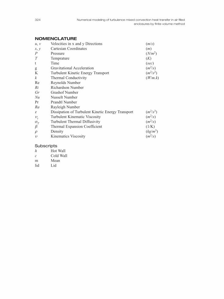
NOMENCLATUREu, v Velocities in x and y Directions (m/s)x, y Cartesian Coordinates (m)P Pressure (N/m2)T Temprature (K)t Time (sec)g Gravitational Acceleration (m2/s)K Turbulent Kinetic Energy Transport (m2/s2)k Thermal Conductivity (W/m.k)Re Reynolds NumberRi Richardson NumberGr Grashof NumberNu Nusselt Number Pr Prandtl NumberRa Rayleigh Numberε Dissipation of Turbulent Kinetic Energy Transport (m2/s3)υt Turbulent Kinematic Viscosity (m2/s)σT Turbulent Thermal Diffusivity (m2/s)β Thermal Expansion Coefficient (1/K) ρ Density (kg/m3)υ Kinematics Viscosity (m2/s)

Subscriptsh Hot Wallc Cold Wallm Meanlid Lid


Numerical modeling of turbulence mixed convection heat transfer in air filled enclosures by finite volume method

Documents