Numerical modeling of self-channeling granular flows and of their levee-channel deposits

Numerical modeling of self-channeling granular flows

and of their levee-channel deposits

A. Mangeney,1,2 F. Bouchut,3 N. Thomas,4 J. P. Vilotte,1 and M. O. Bristeau5

Received 26 January 2006; revised 13 October 2006; accepted 18 December 2006; published 17 May 2007.

[1] When not laterally confined in valleys, pyroclastic flows create their own channelalong the slope by selecting a given flowing width. Furthermore, the lobe-shapeddeposits display a very specific morphology with high parallel lateral levees. A numericalmodel based on Saint Venant equations and the empirical variable friction coefficientproposed by Pouliquen and Forterre (2002) is used to simulate unconfined granular flowover an inclined plane with a constant supply. Numerical simulations successfullyreproduce the self-channeling of the granular lobe and the levee-channel morphology inthe deposits without having to take into account mixture concepts or polydispersity.Numerical simulations suggest that the quasi-static shoulders bordering the flow arecreated behind the front of the granular material by the rotation of the velocity field due tothe balance between gravity, the two-dimensional pressure gradient, and friction. For asimplified hydrostatic model, competition between the decreasing friction coefficient andincreasing surface gradient as the thickness decreases seems to play a key role in thedynamics of unconfined flows. The description of the other disregarded components of thestress tensor would be expected to change the balance of forces. The front’s shape appearsto be constant during propagation. The width of the flowing channel and the velocity ofthe material within it are almost steady and uniform. Numerical results suggest thatmeasurement of the width and thickness of the central channel morphology in deposits inthe field provides an estimate of the velocity and thickness during emplacement.

Citation: Mangeney, A., F. Bouchut, N. Thomas, J. P. Vilotte, and M. O. Bristeau (2007), Numerical modeling of self-channeling

granular flows and of their levee-channel deposits, J. Geophys. Res., 112, F02017, doi:10.1029/2006JF000469.

1. Introduction

[2] When not laterally confined in valleys, pyroclasticflows propagate with a tongue shape and subparallel bor-ders, creating their own channel along a slope by selecting agiven flowing width that is strongly dependent on theunderlying topography. Furthermore, the lobe-shapeddeposits exhibit a very specific morphology with parallellateral levees (about 1 m high) enriched in large blockswhile the central channel is lower and composed mainly ofsmaller particles [e.g., Nairn and Self, 1978; Calder et al.,2000; Saucedo et al., 2002; Ui et al., 1999; Rodriguez-Elizarraras et al., 1991; Wilson and Head, 1981]. Suchchanneled flows leaving a levee-channel morphology indeposits on the slope are also observed in very different

environments and for flows involving completely differentmaterials such as landslide deposits on Mars [Mangold et al.,2003; Treiman and Louge, 2004] or submarine landslides[Klaucke et al., 2004]. Although lava flows have a totallydifferent mechanical behavior, similar morphological fea-tures are observed in their deposits [Sakimoto and Gregg,2001; Quareni et al., 2004].[3] Several explanations have been proposed for the

channeling of these unconfined flows and their levee-channel morphology: Bingham rheology leading to lateralstatic zones as is the case for lava flows [Yamamoto et al.,1993; Quareni et al., 2004; Mangold et al., 2003], drainageof the central part of the deposit with static levees [Rowleyet al., 1981] and differential deflation and differentialfluidization of borders during emplacement due to polydis-persity of the particles [Rowley et al., 1981; Wilson andHead, 1981]. The levee-channel morphology observed onMartian landslides was first interpreted as indicating thepresence of water during emplacement [Malin and Edgett,2000]. Similarly, assuming a Bingham rheology, Mangoldet al. [2003] deduced from the analysis of levees that theobserved gullies over large Martian dunes involve flowswith a significant proportion of fluids. On the other hand,Treiman and Louge [2004] refer to dry flows to explainthe levee-channel morphology of Martian gullies. Fieldmeasurements have been performed on such deposits, butthe question remains as to what extent these measurements

JOURNAL OF GEOPHYSICAL RESEARCH, VOL. 112, F02017, doi:10.1029/2006JF000469, 2007ClickHere

for

FullArticle

1UMR 7580, Institut de Physique du Globe de Paris, UniversiteDenis Diderot, CNRS, Paris, France.

2Now at Institute for Nonlinear Science, University of California,San Diego, La Jolla, USA.

3Departement de Mathematique et Applications, Ecole NormaleSuperieure, CNRS, Paris, France.

4Institut Universitaire des Systemes Thermiques Industriels, CNRS,Marseille, France.

5Institut National de Recherche en Informatique et en Automatique,Rocquencourt, France.

Copyright 2007 by the American Geophysical Union.0148-0227/07/2006JF000469$09.00

F02017 1 of 21

provide information on the mechanical properties anddynamics of the flow during emplacement. Which geo-morphologic features (such as width or thickness of thecentral channel or levees) are almost independent withrespect to time and the distance from the supply andtherefore pertinent to characterize the flow?[4] Laboratory experiments show that the channeling of

unconfined flows and the formation of a levee-channelmorphology in deposits may be explained by referring todry granular flows alone [e.g., McDonald and Anderson,1996; Felix and Thomas, 2004]. The channeling and theformation of levees are strongly related to the free lateralboundaries and to the highly unsteady stopping stage.However, while the steady laterally uniform flow regimeof confined granular materials along inclined planes hasbeen largely characterized [Gray et al., 1999; Pouliquen,1999], the behavior of granular materials under unsteadyand nonuniform conditions is still an open question. Theexperiments of Felix and Thomas [2004] on unconfined drygranular flows over an inclined plane show that the forma-tion of levees results from the combination of lateral staticzones on each border of the flow (shoulders) and thedrainage of the central part of the flow after the supplystops. Particle segregation features are also created duringthe flow, corresponding to those observed in the deposits ofpyroclastic flows. When the range of sizes of the polydis-perse material is reduced, the morphology is smoothed butnever reaches a flat surface [Felix and Thomas, 2004].However, a perfectly monodispersed material could not beused in experimental work, and it is therefore possible thatpolydispersity is a necessary condition for the formation ofthe levee-channel morphology. Moreover, it is uncertainwhether this morphology can be obtained without assumingBingham rheology, for example using a Coulomb frictionlaw, better suited to describing the flow of dry granularmatter [see, e.g., Hutter et al., 1995]. It is also unknownhow the shoulders channeling the flow are created and if theassociated spatial nonuniformity is linked to the hystereticcharacter of the granular material, i.e., its capacity to beeither in a static or flowing state depending on the history ofthe dynamics.[5] The aim of this paper is to shed light on these

questions by assessing whether a simple depth-averagedmodel based on Saint Venant equations and Coulomb typefriction is able to reproduce the complex behavior ofunconfined granular flows with channel formation andlevee-channel morphology in deposits. A simple hydrostaticmodel involving the empirical variable friction coefficientproposed by Pouliquen and Forterre [2002] is used here. Asthe other friction laws proposed in the literature for drygranular flows, Pouliquen and Forterre’s empirical flow ruleis obviously oversimplified to reproduce the natural com-plexity where polydisperse, multiphase materials are in-volved. The following simulations strongly depend on thepeculiar features of this empirical friction law. The casetreated in this paper, namely dry granular flows withoutpolydispersity effects over inclined plane, is very simpleand therefore quite different from typical geophysical casessuch as pyroclastic flows and debris flows involving effectslike grain size segregation and variable liquefaction orfluidization [e.g., Iverson and Vallance, 2001]. The question

addressed here is whether self-channeling flows and levee-channel morphology can be obtained for this simple case.[6] Simple continuum hydrodynamic models, based on the

long-wave approximation (hereafter called LWA) [Savageand Hutter, 1989] and Saint Venant equations, have beenshown to reproduce the basic features of both experimentaldense granular flows along inclined planes and geologicalflows over real topographies [e.g., Denlinger and Iverson,2001;Naaim et al., 1997; Pastor et al., 2002;McDougall andHungr, 2004; Pouliquen and Forterre, 2002; Mangeney-Castelnau et al., 2003; Pitman et al., 2003; Denlinger andIverson, 2004; Iverson et al., 2004; Sheridan et al., 2007;Lucas and Mangeney, 2007]. Continuum models areexpressed in terms of the change of the vertically averagedvelocity field and of the associated vertical length scale h, i.e.,the avalanche thickness, and describe hydrostatic imbalance[Mangeney-Castelnau et al., 2003] or nonhydrostatic plas-ticity and friction effects [Savage and Hutter, 1989]. Themodels assume an averaged friction dissipation describedphenomenologically by Coulomb0s friction law with aconstant [e.g., Hutter et al., 1995; Naaim et al., 1997] orvelocity- and thickness-dependent [Pouliquen, 1999;Douady et al., 1999] friction coefficient. More sophisticatedmodels have been recently proposed by Denlinger andIverson [2004] based on Mohr-Coulomb plasticity theory.Although the friction law describing the behavior of steadyflows has been relatively well refined by laboratory experi-ments, the behavior of a granular mass at small Froudenumbers (i.e., at low velocities) is still an open question.Hysteresis is an important characteristic of granular slopestability. Indeed, a granular slope starts to flow when itsinclination reaches a typical avalanche angle qa and comesto rest once its slope reaches another so-called repose angleqr < qa. The hysteretic behavior occurs for inclination anglesq 2[qr, qa] [e.g., Pouliquen and Forterre, 2002; Daerr andDouady, 1999]. The metastability of a granular slope in thisrange of angles has been shown to be very complex andrequires a biphasic description of strong and weak contactnetworks in the granular pile [Deboeuf et al., 2005a,2005b]. In the macroscopic depth-averaged formulationinherent to the long-wave approximation, the empiricdescription of this metastability remains uncertain. Still,the formation of channeling flows with the construction ofnearly static shoulders as well as the existence of leveesare likely to be strongly related to the behavior of granularmaterials near the stopping or destabilization phases. Becauseunconfined flows continuously juggle between static andflowing conditions, their numerical simulation can be usedto improve the macroscopic description of the metastablebehavior of granular flows which is still an open question.[7] We first briefly describe, in section 2, the experimen-

tal results that motivated this study. After a description ofthe model and the flow law in section 3, a simulation ofexperimental results of confined granular flow over aninclined plane with constant supply and its deposit afterstopping the supply is described in section 4 in order tocheck the model in a configuration much simple than thecase of free-boundary flows. A numerical simulation of thechanneling process and the formation of levees is performedin section 5, providing new insight into the experimentalobservations based on a qualitative comparison between

F02017 MANGENEY ET AL.: NUMERICAL SIMULATION OF LEVEES

2 of 21

F02017

experimental and numerical results. In section 6, the dy-namics of the channeling flows and the forces involved areinvestigated to shed light on the mechanism generating thecomplex behavior of unconfined flows.

2. Experimental Evidence

[8] Felix and Thomas [2004] have shown that unconfinedflows of dry granular material over a rough inclined planewith a constant supply reach a steady state, after which thefront propagates at a constant velocity, the thickness isquasi-uniform and constant with time and the width of theflow is uniform. The structure of unconfined flow has beenshown to be separated into a flowing central channel andtwo static shoulders on each border of the channel. As thesupply stops, the thickness of the channel decreases whilethe thickness of the static shoulders remains unchanged,leading to a deposit with a levee-channel morphology. Glassbeads of diameter 300–400 mm have been used in theexperiments with initial flux varying from 6 g s�1 to 34 gs�1 over an inclined plane 2 m long and 80 cm wide, withslope angles in the range [25�,29�]. Taking a closer look atthe dynamics of unconfined flow, recent experiments haveshown that granular flow slowly enlarges while its thicknessdecreases if the supply is maintained for a long duration[Deboeuf et al., 2006].[9] Although these studies mention the effect of polydis-

persity, it has not been determined whether segregation is anecessary condition to obtain levees and static shoulders.Moreover, these studies do not provide the precise velocityfield within the flow and do not explain the formation ofstatic shoulders at the rear of the front. It seems that thedynamics at the front determine the width but this mecha-nism has not been investigated. Consequently, no conditioncan be deduced for the determination of the width, thicknessand velocity of the flow for a given flux. In the following,we simulate this type of experiment numerically using along-wave approximation model. We investigate to whatextent such a model is able to shed light on these questions.

3. Model

3.1. Mass and Momentum Conservation

[10] Depth-averaged continuum models have been shownto be useful in reproducing the basic behavior of the flow onsloping topography under experimental or natural condi-tions [e.g., Denlinger and Iverson, 2001; Naaim et al.,1997; Pouliquen and Forterre, 2002; Mangeney-Castelnauet al., 2003, 2005; Pitman et al., 2003]. These models arebased on the long-wave approximation, which is appropri-ate for granular flows over inclined topography given thatthe characteristic length in the flow direction is much largerthan the vertical length, i.e., the avalanche thickness,thereby satisfying the hydrostatic assumption.[11] A new model has recently been derived by Bouchut

and Westdickenberg [2004] for gravity driven shallow waterflow over an arbitrary two-dimensional (2-D) topography.The model is written in an arbitrary coordinate system forshallow flow over a topography with small curvature.Dimensional analysis has been performed by Bouchut andWestdickenberg [2004] in a manner similar to that of Hutterand coworkers. The overall idea is to develop the equations

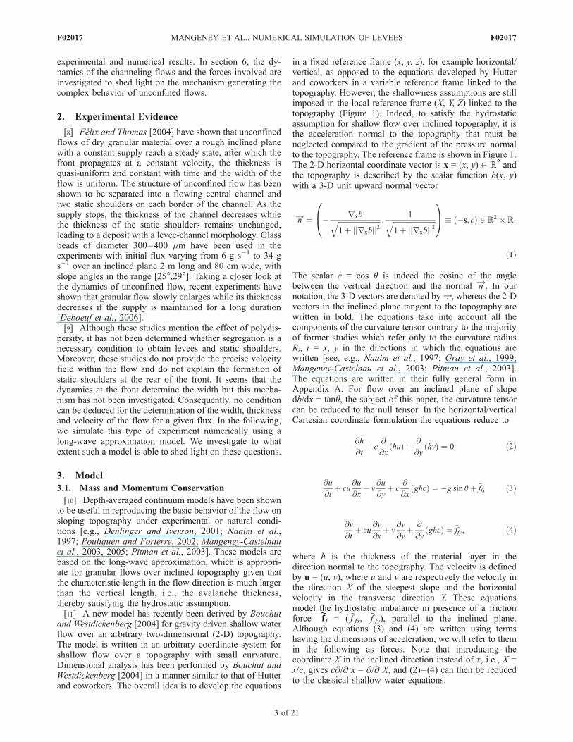
in a fixed reference frame (x, y, z), for example horizontal/vertical, as opposed to the equations developed by Hutterand coworkers in a variable reference frame linked to thetopography. However, the shallowness assumptions are stillimposed in the local reference frame (X, Y, Z) linked to thetopography (Figure 1). Indeed, to satisfy the hydrostaticassumption for shallow flow over inclined topography, it isthe acceleration normal to the topography that must beneglected compared to the gradient of the pressure normalto the topography. The reference frame is shown in Figure 1.The 2-D horizontal coordinate vector is x = (x, y) 2 R

2 andthe topography is described by the scalar function b(x, y)with a 3-D unit upward normal vector

n!¼ � rxbffiffiffiffiffiffiffiffiffiffiffiffiffiffiffiffiffiffiffiffiffiffiffiffi1þ jjrxbjj2

q ;1ffiffiffiffiffiffiffiffiffiffiffiffiffiffiffiffiffiffiffiffiffiffiffiffi

1þ jjrxbjj2q

0B@1CA �s; cð Þ 2 R

2 � R:

ð1Þ

The scalar c = cos q is indeed the cosine of the anglebetween the vertical direction and the normal n!. In ournotation, the 3-D vectors are denoted by :!, whereas the 2-Dvectors in the inclined plane tangent to the topography arewritten in bold. The equations take into account all thecomponents of the curvature tensor contrary to the majorityof former studies which refer only to the curvature radiusRi, i = x, y in the directions in which the equations arewritten [see, e.g., Naaim et al., 1997; Gray et al., 1999;Mangeney-Castelnau et al., 2003; Pitman et al., 2003].The equations are written in their fully general form inAppendix A. For flow over an inclined plane of slopedb/dx = tanq, the subject of this paper, the curvature tensorcan be reduced to the null tensor. In the horizontal/verticalCartesian coordinate formulation the equations reduce to

@h

@tþ c

@

@xhuð Þ þ @

@yhvð Þ ¼ 0 ð2Þ

@u

@tþ cu

@u

@xþ v

@u

@yþ c

@

@xghcð Þ ¼ �g sin qþ ~ffx ð3Þ

@v

@tþ cu

@v

@xþ v

@v

@yþ @

@yghcð Þ ¼ ~ffy; ð4Þ

where h is the thickness of the material layer in thedirection normal to the topography. The velocity is definedby u = (u, v), where u and v are respectively the velocity inthe direction X of the steepest slope and the horizontalvelocity in the transverse direction Y. These equationsmodel the hydrostatic imbalance in presence of a frictionforce

~f f = ( ~f fx, ~f fy), parallel to the inclined plane.

Although equations (3) and (4) are written using termshaving the dimensions of acceleration, we will refer to themin the following as forces. Note that introducing thecoordinate X in the inclined direction instead of x, i.e., X =x/c, gives c@/@ x = @/@ X, and (2)–(4) can then be reducedto the classical shallow water equations.

F02017 MANGENEY ET AL.: NUMERICAL SIMULATION OF LEVEES

3 of 21

F02017

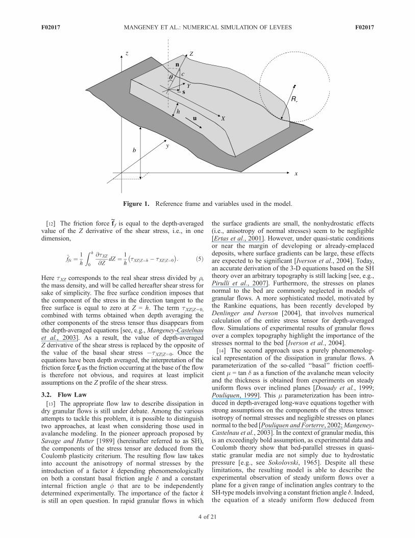
[12] The friction force~f f is equal to the depth-averaged

value of the Z derivative of the shear stress, i.e., in onedimension,

~ffx ¼1

h

Z h

0

@tXZ@Z

dZ ¼ 1

htXZjZ¼h � tXZjZ¼0

�: ð5Þ

Here tXZ corresponds to the real shear stress divided by r,the mass density, and will be called hereafter shear stress forsake of simplicity. The free surface condition imposes thatthe component of the stress in the direction tangent to thefree surface is equal to zero at Z = h. The term tXZjZ=0,combined with terms obtained when depth averaging theother components of the stress tensor thus disappears fromthe depth-averaged equations [see, e.g.,Mangeney-Castelnauet al., 2003]. As a result, the value of depth-averagedZ derivative of the shear stress is replaced by the opposite ofthe value of the basal shear stress �tXZjZ=0. Once theequations have been depth averaged, the interpretation of thefriction force ff as the friction occurring at the base of the flowis therefore not obvious, and requires at least implicitassumptions on the Z profile of the shear stress.

3.2. Flow Law

[13] The appropriate flow law to describe dissipation indry granular flows is still under debate. Among the variousattempts to tackle this problem, it is possible to distinguishtwo approaches, at least when considering those used inavalanche modeling. In the pioneer approach proposed bySavage and Hutter [1989] (hereinafter referred to as SH),the components of the stress tensor are deduced from theCoulomb plasticity criterium. The resulting flow law takesinto account the anisotropy of normal stresses by theintroduction of a factor k depending phenomenologicallyon both a constant basal friction angle d and a constantinternal friction angle f that are to be independentlydetermined experimentally. The importance of the factor kis still an open question. In rapid granular flows in which

the surface gradients are small, the nonhydrostatic effects(i.e., anisotropy of normal stresses) seem to be negligible[Ertas et al., 2001]. However, under quasi-static conditionsor near the margin of developing or already-emplaceddeposits, where surface gradients can be large, these effectsare expected to be significant [Iverson et al., 2004]. Today,an accurate derivation of the 3-D equations based on the SHtheory over an arbitrary topography is still lacking [see, e.g.,Pirulli et al., 2007]. Furthermore, the stresses on planesnormal to the bed are commonly neglected in models ofgranular flows. A more sophisticated model, motivated bythe Rankine equations, has been recently developed byDenlinger and Iverson [2004], that involves numericalcalculation of the entire stress tensor for depth-averagedflow. Simulations of experimental results of granular flowsover a complex topography highlight the importance of thestresses normal to the bed [Iverson et al., 2004].[14] The second approach uses a purely phenomenolog-

ical representation of the dissipation in granular flows. Aparameterization of the so-called ‘‘basal’’ friction coeffi-cient m = tan d as a function of the avalanche mean velocityand the thickness is obtained from experiments on steadyuniform flows over inclined planes [Douady et al., 1999;Pouliquen, 1999]. This m parameterization has been intro-duced in depth-averaged long-wave equations together withstrong assumptions on the components of the stress tensor:isotropy of normal stresses and negligible stresses on planesnormal to the bed [Pouliquen and Forterre, 2002;Mangeney-Castelnau et al., 2003]. In the context of granular media, thisis an exceedingly bold assumption, as experimental data andCoulomb theory show that bed-parallel stresses in quasi-static granular media are not simply due to hydrostaticpressure [e.g., see Sokolovski, 1965]. Despite all theselimitations, the resulting model is able to describe theexperimental observation of steady uniform flows over aplane for a given range of inclination angles contrary to theSH-type models involving a constant friction angle d. Indeed,the equation of a steady uniform flow deduced from

Figure 1. Reference frame and variables used in the model.

F02017 MANGENEY ET AL.: NUMERICAL SIMULATION OF LEVEES

4 of 21

F02017

equation (3) combined with the Coulomb friction law (7)described in the following reads

m ¼ tan q; ð6Þ

indicating that the friction force exactly balances the forceof gravity. This equilibrium is also obtained with SH’sequations even if the stresses normal to the bed areintroduced in a way similar to that of Iverson and Denlinger[2001]. In fact, in the case of steady uniform flow @h/@x and@h/@y are equal to zero and the terms related to anisotropyof normal stresses or stresses on planes normal to the beddisappear.[15] However, the physical basis of this m parameteriza-

tion is still an open question. In particular, this parameter-ization is obtained by assuming that all the dissipation isdescribed by the term

~f f in equations (3) and (4). The

question, however, is: does this relation hold only becausethe other components of the stress tensor or the friction atthe lateral walls are neglected or because the dissipation ingranular flows is more complicated than the proposedCoulomb-type models? Despite all these uncertainties, wetry here, in a first attempt to model the process of leveeformation by unconfined granular flows, to reproduce theobserved channeling of the flow and the levee-channelmorphology by simply using this m parameterization. Theidea is to analyze the balance of the forces that governs themechanics of self-channeling flows when this phenomeno-logical representation of dissipation effects is introduced inthe model. All the limitations due to the strong assumptionsrelated to the disregarded components of the stress tensorhave to be kept in mind when analyzing the followingresults.[16] Unlike fluids, granular materials can sustain a given

stress without deforming. The transition between a staticstate (u = 0) and a flowing state is generally simply modeledin depth-averaged models by introducing a Coulomb thresh-old sc. The motion is allowed only if the norm of the drivingforces jj~f fjj exceeds the Coulomb threshold [Mangeney-Castelnau et al., 2003]. In the model (3)– (4),

~f f is

expressed as

jj ~f f jj sc )~f f ¼ �gcm u

jjujjjj ~f f jj < sc ) u ¼ 0;

ð7Þ

where sc = gcm. When the material exceeds the Coulombthreshold, the Coulomb friction law states that whenflowing, the friction force has a direction opposite to theaveraged tangential velocity field and the amplitude of thefriction force is governed by the total overall pressure andthe friction coefficient m. The friction force

~f f is multivalued

for (u, v) = (0, 0) when the flow history is not known. Forthis reason, the friction has been regularized numerically asdescribed in Appendix B (equations (B12) and (B16)). As aresult, for small velocities, the direction of the friction isgiven by the driving forces related to the h gradient andgravity. It is well known that the failure surface developswithin the granular mass at the initiation of the flow and thatthe arrest phase involves both a horizontal and a verticalpropagation of the transition between static and flowingmaterials. The above classical approach (7) to describe the

initiation or stopping of the flow by simply referring to the‘‘basal’’ coefficient of friction is difficult to justify whenboth basal and internal dissipation are taken into account inthe model.[17] Near the transition between the static (jammed) and

the flowing (unjammed) state, the behavior of granularmaterial is still an open question. In this so-called metasta-ble regime, the jammed state of the granular material isconditionally stable and an avalanche can be triggered byperturbations of finite amplitude [Daerr and Douady, 1999].The different characteristic angles of stability of granularsystems reflect this metastability. In the case studied here,where quasi-static zones develop near the margins of thegranular lobe, the behavior in the metastable regime isexpected to play a key role in the dynamics. Is it necessaryto take into account two different friction angles correspondingto the avalanche and repose angles to simulate self-channelingflows? Is the metastable regime involved during the formationof self-channeling flows?[18] These questions will be investigated here by using

the m parameterization proposed by [Pouliquen and Forterre,2002] which takes into account the typical hysteresis behaviorof granular matter. Let us recall here the main features of thisphenomenological approach. Steady uniform flows overrough bedrock have been observed experimentally for a rangeof inclination angles, making it possible to identify a scalinglaw relating the thickness and mean velocity of the flow[Pouliquen, 1999]. This scaling law or flow rule involvestwo empirical functions that are expected to contain funda-mental information on the friction properties of the materialand of its interaction with the rough plane: (1) the functionrelating the slope angle q of an inclined plane to the thicknessstaying on the plane hstop(q) and (2) the function relating theslope angle q to the minimum thickness of an initially at restgranular layer necessary to generate a flow on the same planehstart(q).[19] These empirical functions

hstop qð Þ ¼ Ltan d2 � tan qtan q� tan d1

ð8Þ

hstart qð Þ ¼ Ltan d4 � tan qtan q� tan d3

ð9Þ

involve the parameters di and L that can be deduced fromexperiments by fitting the curves hstop(q) and hstart(q) forinclination angle q 2 [d1, d2] and q 2 [d3, d4], respectively.The parameters di correspond to the limiting angles forwhich these measurements can be done. As an example, foran inclination angle of the plane q = d1, the static thicknesshstop diverges and for q = d2, there is no deposit left on theplane, i.e., hstop = 0. We use here d1 = 22�, d2 = 34�, d3 =23�, d4 = 36�, and L = 8 � 10�4 m which are characteristicvalues of the parameters determined in the experiments ofFelix and Thomas [2004]. With these parameters hstop =2.6743 � 10�3m for q = 25� so that hstop � 7d, where d isthe typical grain diameter in the experiments and hstart =4.9767 � 10�3m with hstart � hstop � 6d (hstart/hstop =1.861).[20] In the domain q 2 [d1, d2], the function hstop has been

shown to be an appropriate scaling parameter providing a

F02017 MANGENEY ET AL.: NUMERICAL SIMULATION OF LEVEES

5 of 21

F02017

relation between the thickness of the flow h and the Froudenumber Fr = jj u jj/

ffiffiffiffiffigh

pfor steady uniform flow

hstop ¼ bh

Fr þ að10Þ

whatever the size of the beads. The values of b = 0.136 anda = 0 have been measured for glass beads (b = 0.65 and a =0.136 is found for sand particles) [Forterre and Pouliquen,2003]. We use here the parameters measured for glassbeads, typical of the material used in the experiments ofFelix and Thomas [2004]. Relation (10) is defined whensteady flow is possible, i.e., when h > hstop or equivalentlywhen Fr > b.[21] In steady uniform flows (Fr > b), the friction

coefficient m is related to the slope angle q owing to therelation (6). Using (8) and (6), the friction coefficient can beexpressed as a function of hstop

m ¼ mstop hstop �

¼ tan d1 þ tan d2 � tan d1ð Þ 1hstopL

þ 1: ð11Þ

Owing to relation (10), m can be related to the thickness hand the Froude number Fr of the flow. On the other hand,for a uniform granular layer of thickness h = hstart, initiallyat rest (Fr = 0) on a plane with inclination, equations (6) and(9) give

m ¼ mstart hstartð Þ ¼ tan d3 þ tan d4 � tan d3ð Þ 1hstartL

þ 1: ð12Þ

The behavior at 0 < Fr � b corresponds to metastableconditions, for which no measurements were available untilvery recently. An empirical ad hoc fit has been proposedby Pouliquen and Forterre [2002] to relate the behavior atFr > b to the measurements at Fr = 0 corresponding todestabilization from rest. Note that recent studies have beenperformed by Da Cruz [2004] providing insight into theflow law at small Froude numbers, i.e., 0 < Fr � b.[22] To sum up, the empirical friction coefficient m(h, Fr)

proposed by Pouliquen and Forterre [2002] and used hereis defined as

if Fr > b

m h;Frð Þ ¼ tan d1 þ tan d2 � tan d1ð Þ 1bhFrL

þ 1; ð13Þ

if Fr = 0

m h;Frð Þ ¼ tan d3 þ tan d4 � tan d3ð Þ 1hLþ 1

; ð14Þ

if 0 � Fr < b

m h;Frð Þ ¼ mstart hð Þ þ Fr

b

� x

mstop hð Þ � mstart hð Þ� �

; ð15Þ

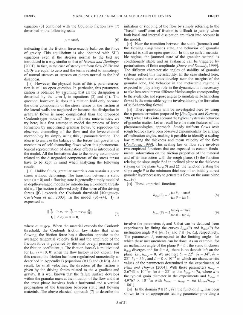
where x is a small parameter (here x = 10�3). The coloredsurface represented in Figure 2 shows that for Fr > b thecoefficient of friction m increases when the Froude numberincreases and when h decreases. For a given value of h, thecoefficient of friction is almost constant in the metastableregime 0 � Fr < b and sharply increases near Fr = 0.[23] The friction is then modeled by equation (7) with a

variable Coulomb threshold sc = gcm(h, Fr) with m definedjust above by equations (13)–(15). The friction modelallows a mass initially at rest to flow when the drivingforces due to surface slope and gravity exceed the Coulombthreshold related to mstart. Similarly, the mass stops when thedriving forces due to inertia, surface slope and gravity dropbelow the Coulomb threshold related to mstop. The model istherefore able to describe the hysteretic behavior of granularflows. In the case studied here, the ‘‘static’’ and ‘‘dynamic’’friction coefficients are in the range mstart 2 [0.42, 0.73] andmstop 2 [0.40, 0.67] respectively. Note that the flow law usedhere does not describe a constant value of the basal stress asproposed by Dade and Huppert [1998] or Kelfoun andDruitt [2005] but rather a constant friction coefficient insteady state owing to relation (6).

3.3. Numerical Method

[24] The numerical method used to solve the hyperbolicsystem (2)–(4) and (7) relies on a finite volume formulationtogether with the hydrostatic reconstruction scheme devel-oped by Audusse et al. [2004] for Saint Venant models, andon the apparent topography approach of Bouchut [2004] todeal with friction. This numerical model has recently beensuccessfully applied to the simulation of the collapse of agranular column over a horizontal plane by Mangeney-Castelnau et al. [2005]. This finite volume scheme providessecond-order accuracy, in contrast with the first-ordermethod

Figure 2. Friction coefficient defined by the empiricalrelation m(h, Fr) (colored surface, equations (13)–(15)).The point (Fr = b, h = 2.2, m = 0) has been represented inblack in order to show the extension of the metastableregime 0 < Fr < b. The colored lines represent the valuesof (m(t), h(t)/hstop, Fr(t)) as time evolves at a fixed point A1

(x = 1.2 m, y = 0.1 cm) situated at the middle of the plane,for the simulation of confined flow described in section 4with a boundary flux Q1 = 2 � 10�4 m2 s�1 (white line) andQ2 = 4 � 10�4 m2 s�1 (magenta line).

F02017 MANGENEY ET AL.: NUMERICAL SIMULATION OF LEVEES

6 of 21

F02017

used by Mangeney-Castelnau et al. [2003] and based on akinetic scheme. The method used is described in more detailin Appendix B and in the work by Bouchut [2004].[25] Alternative methods have recently been proposed by

Denlinger and Iverson [2004], based on a combination offinite volume and finite element schemes, and by Pitman etal. [2003], based on a finite volume scheme together withan adaptive grid. A comparison of these different methodswould be of interest but is beyond the scope of this paper.[26] For our purpose, we performed a series of numerical

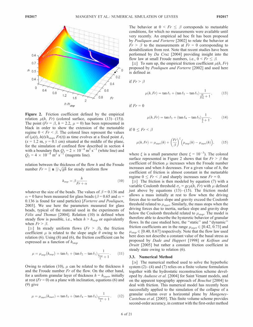
experiments on a two-dimensional regular grid with 400 �100 points for the simulation of confined flows (section 4)and 400� 300 points for unconfined flows (sections 5 and 6).At the upper boundary of the numerical model a flux anda thickness are imposed while free boundary conditionsare prescribed on the other boundaries of the domain(Figures 3a and 3b). The stopping of the supply is imposednumerically by prescribing a zero flux and thickness at theleft boundary of the domain (Figure 3c).

4. Simulation of Confined Flow

[27] To test the numerical model proposed here and toobtain an idea of its behavior, we will first simulate a casemuch simpler than that of unconfined flow: the confined flowof a transversally uniform layer of granular material over aninclined plane with a constant supply all across the plane in itsupper part. This laboratory experiment, first performed byPouliquen [1999], is the basis of the friction law presented

above. Numerical simulations using this empirical frictionlaw have been shown to be able to reproduce granularbehavior in unsteady situations [Pouliquen and Forterre,2002; Mangeney-Castelnau et al., 2003]. As in the work ofMangeney-Castelnau et al. [2003], with a numerical modelbased on a first-order kinetic scheme, the ability of themodel to reach the right steady state and to calculate thethickness h = hstop once the supply is stopped is investi-gated here. Furthermore, the behavior of this flow and itsstopping after the supply is shutdown gives a comparisontool when simulating the more complex case of freeboundary channeling flow.[28] Two numerical experiments are performed by im-

posing at the upper boundary, over the full width of a planewith an inclination angle q = 25�: (1) a flux Q1 = hu =2.10�4m2 s�1 (Figures 4a and 4c) and (2) a flux Q2 = hu =4.10�4m2 s�1 (Figures 4b and 4d). Wall boundary conditionsare imposed on the lateral part of the numerical domain. Thenumerical domain is Lx = 2.2 m long and Ly = 20 cm wide.The supply is kept constant until a steady uniform regimeis reached. Then, the supply is stopped at ts = 70 s and ts =60 s in the simulation with the input flux Q1 and Q2,respectively. Finally, the final thickness of the deposit onthe inclined plane is measured.

4.1. Evolution to Steady State

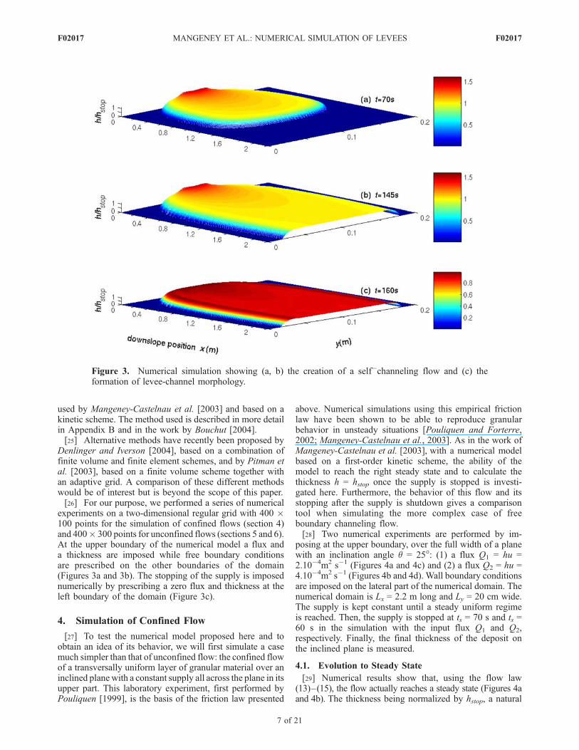
[29] Numerical results show that, using the flow law(13)–(15), the flow actually reaches a steady state (Figures 4aand 4b). The thickness being normalized by hstop, a natural

Figure 3. Numerical simulation showing (a, b) the creation of a self�channeling flow and (c) theformation of levee-channel morphology.

F02017 MANGENEY ET AL.: NUMERICAL SIMULATION OF LEVEES

7 of 21

F02017

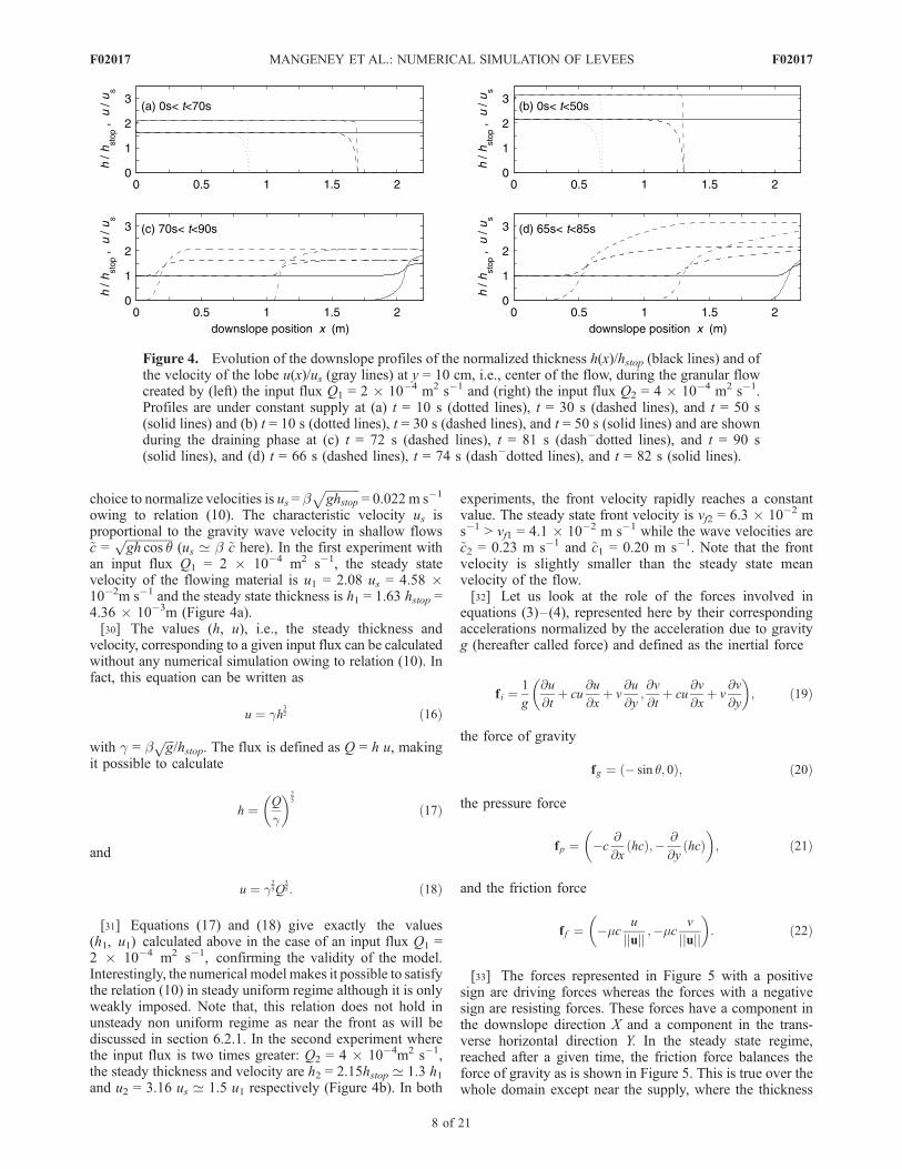
choice to normalize velocities is us = bffiffiffiffiffiffiffiffiffiffiffighstop

p= 0.022m s�1

owing to relation (10). The characteristic velocity us isproportional to the gravity wave velocity in shallow flows~c =

ffiffiffiffiffiffiffiffiffiffiffiffiffiffiffigh cos q

p(us ’ b ~c here). In the first experiment with

an input flux Q1 = 2 � 10�4 m2 s�1, the steady statevelocity of the flowing material is u1 = 2.08 us = 4.58 �10�2m s�1 and the steady state thickness is h1 = 1.63 hstop =4.36 � 10�3m (Figure 4a).[30] The values (h, u), i.e., the steady thickness and

velocity, corresponding to a given input flux can be calculatedwithout any numerical simulation owing to relation (10). Infact, this equation can be written as

u ¼ gh32 ð16Þ

with g = bffiffiffig

p/hstop. The flux is defined as Q = h u, making

it possible to calculate

h ¼ Q

g

� 25

ð17Þ

and

u ¼ g25Q

35: ð18Þ

[31] Equations (17) and (18) give exactly the values(h1, u1) calculated above in the case of an input flux Q1 =2 � 10�4 m2 s�1, confirming the validity of the model.Interestingly, the numerical model makes it possible to satisfythe relation (10) in steady uniform regime although it is onlyweakly imposed. Note that, this relation does not hold inunsteady non uniform regime as near the front as will bediscussed in section 6.2.1. In the second experiment wherethe input flux is two times greater: Q2 = 4 � 10�4m2 s�1,the steady thickness and velocity are h2 = 2.15hstop ’ 1.3 h1and u2 = 3.16 us ’ 1.5 u1 respectively (Figure 4b). In both

experiments, the front velocity rapidly reaches a constantvalue. The steady state front velocity is vf2 = 6.3 � 10�2 ms�1 > vf1 = 4.1 � 10�2 m s�1 while the wave velocities are~c2 = 0.23 m s�1 and ~c1 = 0.20 m s�1. Note that the frontvelocity is slightly smaller than the steady state meanvelocity of the flow.[32] Let us look at the role of the forces involved in

equations (3)–(4), represented here by their correspondingaccelerations normalized by the acceleration due to gravityg (hereafter called force) and defined as the inertial force

f i ¼1

g

@u

@tþ cu

@u

@xþ v

@u

@y;@v

@tþ cu

@v

@xþ v

@v

@y

� ; ð19Þ

the force of gravity

fg ¼ � sin q; 0ð Þ; ð20Þ

the pressure force

fp ¼ �c@

@xhcð Þ;� @

@yhcð Þ

� ; ð21Þ

and the friction force

f f ¼ �mcu

jjujj ;�mcv

jjujj

� : ð22Þ

[33] The forces represented in Figure 5 with a positivesign are driving forces whereas the forces with a negativesign are resisting forces. These forces have a component inthe downslope direction X and a component in the trans-verse horizontal direction Y. In the steady state regime,reached after a given time, the friction force balances theforce of gravity as is shown in Figure 5. This is true over thewhole domain except near the supply, where the thickness

Figure 4. Evolution of the downslope profiles of the normalized thickness h(x)/hstop (black lines) and ofthe velocity of the lobe u(x)/us (gray lines) at y = 10 cm, i.e., center of the flow, during the granular flowcreated by (left) the input flux Q1 = 2 � 10�4 m2 s�1 and (right) the input flux Q2 = 4 � 10�4 m2 s�1.Profiles are under constant supply at (a) t = 10 s (dotted lines), t = 30 s (dashed lines), and t = 50 s(solid lines) and (b) t = 10 s (dotted lines), t = 30 s (dashed lines), and t = 50 s (solid lines) and are shownduring the draining phase at (c) t = 72 s (dashed lines), t = 81 s (dash�dotted lines), and t = 90 s(solid lines), and (d) t = 66 s (dashed lines), t = 74 s (dash�dotted lines), and t = 82 s (solid lines).

F02017 MANGENEY ET AL.: NUMERICAL SIMULATION OF LEVEES

8 of 21

F02017

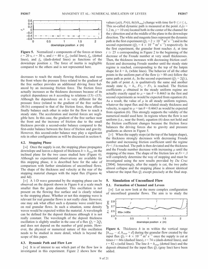
decreases to reach the steady flowing thickness, and nearthe front where the pressure force related to the gradient ofthe free surface provides an additional driving force bal-anced by an increasing friction force. The friction forceactually increases as the thickness decreases because of itsexplicit dependence on h according to relations (13)–(15).Although the dependence on h is very different for thepressure force (related to the gradient of the free surface@h/@x) compared to that of the friction force, these effectsfinally balance each other in order for the flow to reach asteady state. The acceleration and inertial forces are negli-gible here. In this case, the gradient of the free surface nearthe front and the increase of friction due to the smallthickness provide a second-order balance compared to thefirst-order balance between the force of friction and gravity.However, this second-order balance may play a significantrole in other configurations as will be discussed in section 6.

4.2. Stopping Phase

[34] Once the supply is cut, the stopping phase propagatesdownslope and leaves a deposit of thickness h ’ hstop on theinclined plane for the two cases studied here (Figure 6).Although no experimental observations are available forthis stopping phase, it is described here for the sake ofcomparison with further simulations of unconfined flows.The shape of the thickness and velocity at the rear of thestopping material changes with the input flux (Figures 4cand 4d).[35] A 1-D wave generated by the stopping phase can be

observed on the deposit shown in Figure 6 at a scale muchsmaller than the grain diameter. This oscillation is notpresent on the flowing free surface and is clearly relatedto the stopping phase. Whether or not this stopping wave isrelevant for real granular flows is not really clear. However,one may ask what effect such a dynamic wave could haveon real granular flows. In such a situation, some densitywaves would be expected within the material. Awavelengthcan be defined for the deposit thickness although it is notreally constant. The wavelength of the deposit thicknessoscillation is slightly smaller in the case of a flux Q2 = 2Q1

and does not depend on the number of grid points. How-ever, the physical or numerical nature of this oscillationneeds to be studied in more detail, which is beyond thescope of this paper.

4.3. Dynamic Path and Flow Law

[36] It is of interest to see which part of the flow law isinvestigated in this experiment. Figure 2 shows how the

values (m(t), Fr(t), h(t)/hstop) change with time for 0 � t� ts.This so-called dynamic path is measured at the point A1(x =1.2 m, y = 10 cm) located both in the center of the channel forthe y direction and at the middle of the plane in the downslopedirection. The white andmagenta lines represent the dynamicpath in the first experiment (Q1 = 2� 10�4 m2 s�1) and in thesecond experiment (Q2 = 4 � 10�4 m2 s�1) respectively. Inthe first experiment, the granular front reaches A1 at timet ’ 25 s corresponding in Figure 2 to the beginning of thedecrease of the Froude number at very small thicknesses.Then, the thickness increases with decreasing friction coef-ficient and decreasing Froude number until the steady stateregime is reached, corresponding to the top of the hatpinshape for h = h1 (white lines). The behavior of all the otherpoints in the uniform part of the flow (x > 80 cm) follow thesame path as point A1. In the second experiment (Q2 = 2Q1),the path of point A1 is qualitatively the same and anothersteady state h2 > h1, Fr2 > Fr1 is reached. The frictioncoefficients m obtained in the steady uniform regime areactually exactly equal to m = tan q = 0.4663 in the first andsecond experiments as would be expected from equation (6).As a result, the value of m in all steady uniform regimes,whatever the input flux and the related steady thickness andvelocity, is equal to m = tan q = 0.4663 as would be expectedfrom equation (6). This strongly supports the validity of thenumerical model used here. In regions where the flow is notuniform (i.e., near the front), equation (6) does not hold andthe friction coefficient changes because the friction forcebalances the driving forces due to gravity and pressuregradients as shown in Figure 5.[37] When the supply stops (at the top of the hatpin shape),

the thickness strongly decreases with decreasing Froudenumber and increasing friction coefficient until the regimeFr < b is reached. The path is then deviated and the thicknessand the Froude number decrease with increasing m until thestopping of the mass. The shape of the friction law at Fr < bwill completely determine the way of stopping and must beinvestigated using the new results provided by Da Cruz[2004]. Interestingly, after the supply is cut, the two pathsalmost collapse and the stopping phase is almost identicalwhatever the input flux Q, except precisely at the final stop.

5. Simulation of Unconfined Flow

5.1. Formation of Channel and Levees

[38] Let us now look at the more complex configurationof unconfined granular flows. The aim is to study the

Figure 5. Normalized x components of the forces at timest = 20 s, t = 30 s, and t = 40 s: fpx (solid lines), fgx (dottedlines), and ffx (dash-dotted lines) as functions of thedownslope position x. The force of inertia is negligiblecompared to the others and is not represented here.

Figure 6. Thickness h in m within the vertical range[hstop � d, hstop + d] during the granular flow created by theinput flux Q2 = 4 � 10�4 m2 s�1 once the supply is cut attimes t = 66s (dashed lines), t = 74 s (dash-dotted lines), andt = 82 s (solid lines). The line h = hstop (dotted line) and thedeposit obtained for the input flux Q1 (gray line) have beenadded.

F02017 MANGENEY ET AL.: NUMERICAL SIMULATION OF LEVEES

9 of 21

F02017

channeling process as well as the formation of levee-channel morphology of the deposit. While a detailed com-parison between numerical and experimental results wouldbe of great interest, it is beyond the scope of this paper. Weset the initial and boundary conditions in the range of theexperimental conditions of Felix and Thomas [2004]: at theupper boundary, corresponding to the top of the inclinedplane, a flux Q0 = hu = 2� 10�4m2 s�1 and a width w0 = 4 cmare imposed generating a granular lobe flowing over a planewith inclination angle q = 25�. These values give a fluxQ0 =Q0w0 = 8 � 10�6m3 s�1, leading to a mass flux of 12 g.s�1

for glass beads of density r = 2500 kg m�3 and a meandensity of packing f � 0.6, a typical value for densegranular materials. As in the simulation of confined flows,the numerical domain is Lx = 2.2 m long and Ly = 20 cmwide. The supply is stopped at ts = 145 s and the totalsimulation lasts 160 s. At t = 130 s the front has already leftthe plane, leaving behind a flow quasi-uniform in thedownslope direction for x 1.2 m. At the right boundaryof the domain, i.e., at the end of the plane, free boundaryconditions are imposed (the x derivative of the thickness andvelocity are set to zero).[39] The building of shoulders channeling the flow and the

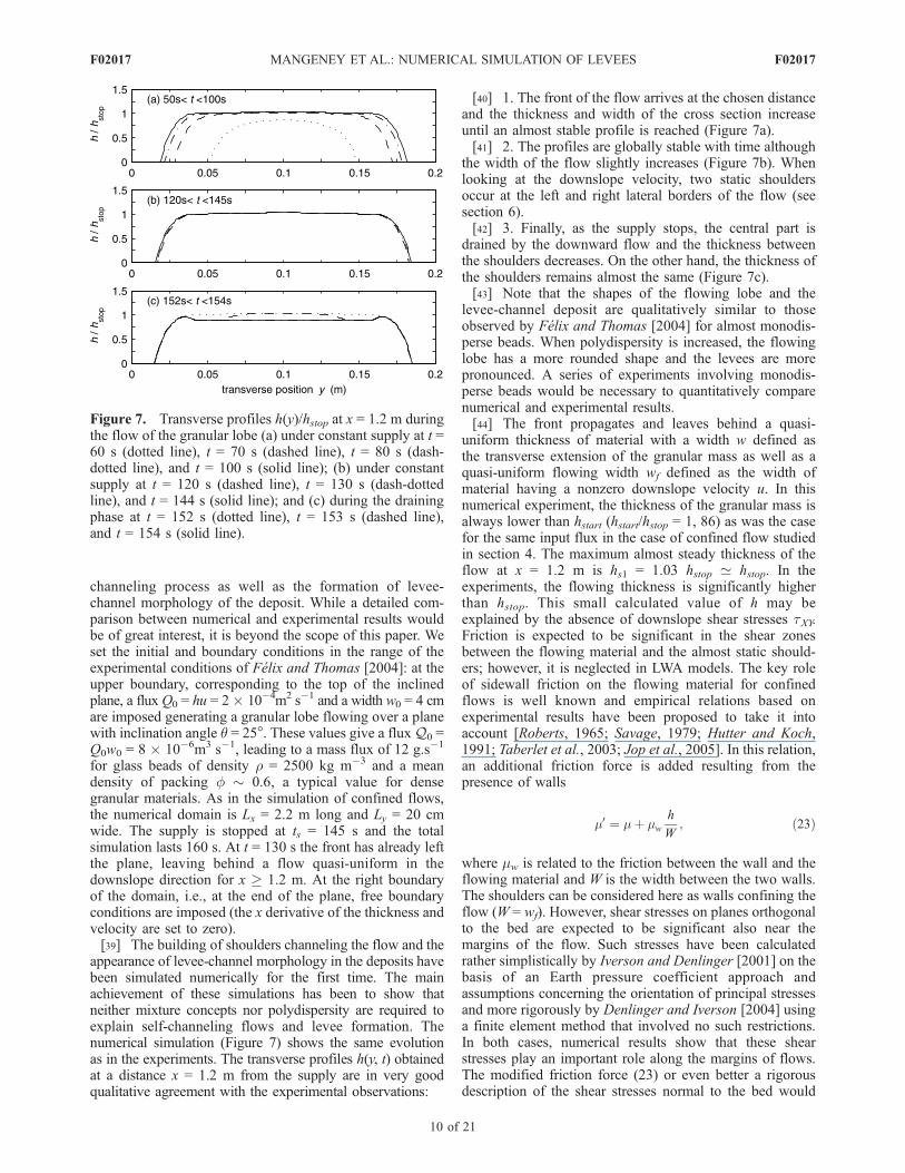
appearance of levee-channel morphology in the deposits havebeen simulated numerically for the first time. The mainachievement of these simulations has been to show thatneither mixture concepts nor polydispersity are required toexplain self-channeling flows and levee formation. Thenumerical simulation (Figure 7) shows the same evolutionas in the experiments. The transverse profiles h(y, t) obtainedat a distance x = 1.2 m from the supply are in very goodqualitative agreement with the experimental observations:

[40] 1. The front of the flow arrives at the chosen distanceand the thickness and width of the cross section increaseuntil an almost stable profile is reached (Figure 7a).[41] 2. The profiles are globally stable with time although

the width of the flow slightly increases (Figure 7b). Whenlooking at the downslope velocity, two static shouldersoccur at the left and right lateral borders of the flow (seesection 6).[42] 3. Finally, as the supply stops, the central part is

drained by the downward flow and the thickness betweenthe shoulders decreases. On the other hand, the thickness ofthe shoulders remains almost the same (Figure 7c).[43] Note that the shapes of the flowing lobe and the

levee-channel deposit are qualitatively similar to thoseobserved by Felix and Thomas [2004] for almost monodis-perse beads. When polydispersity is increased, the flowinglobe has a more rounded shape and the levees are morepronounced. A series of experiments involving monodis-perse beads would be necessary to quantitatively comparenumerical and experimental results.[44] The front propagates and leaves behind a quasi-

uniform thickness of material with a width w defined asthe transverse extension of the granular mass as well as aquasi-uniform flowing width wf defined as the width ofmaterial having a nonzero downslope velocity u. In thisnumerical experiment, the thickness of the granular mass isalways lower than hstart (hstart/hstop = 1, 86) as was the casefor the same input flux in the case of confined flow studiedin section 4. The maximum almost steady thickness of theflow at x = 1.2 m is hs1 = 1.03 hstop ’ hstop. In theexperiments, the flowing thickness is significantly higherthan hstop. This small calculated value of h may beexplained by the absence of downslope shear stresses tXY.Friction is expected to be significant in the shear zonesbetween the flowing material and the almost static should-ers; however, it is neglected in LWA models. The key roleof sidewall friction on the flowing material for confinedflows is well known and empirical relations based onexperimental results have been proposed to take it intoaccount [Roberts, 1965; Savage, 1979; Hutter and Koch,1991; Taberlet et al., 2003; Jop et al., 2005]. In this relation,an additional friction force is added resulting from thepresence of walls

m0 ¼ mþ mw

h

W; ð23Þ

where mw is related to the friction between the wall and theflowing material and W is the width between the two walls.The shoulders can be considered here as walls confining theflow (W = wf). However, shear stresses on planes orthogonalto the bed are expected to be significant also near themargins of the flow. Such stresses have been calculatedrather simplistically by Iverson and Denlinger [2001] on thebasis of an Earth pressure coefficient approach andassumptions concerning the orientation of principal stressesand more rigorously by Denlinger and Iverson [2004] usinga finite element method that involved no such restrictions.In both cases, numerical results show that these shearstresses play an important role along the margins of flows.The modified friction force (23) or even better a rigorousdescription of the shear stresses normal to the bed would

Figure 7. Transverse profiles h(y)/hstop at x = 1.2 m duringthe flow of the granular lobe (a) under constant supply at t =60 s (dotted line), t = 70 s (dashed line), t = 80 s (dash-dotted line), and t = 100 s (solid line); (b) under constantsupply at t = 120 s (dashed line), t = 130 s (dash-dottedline), and t = 144 s (solid line); and (c) during the drainingphase at t = 152 s (dotted line), t = 153 s (dashed line),and t = 154 s (solid line).

F02017 MANGENEY ET AL.: NUMERICAL SIMULATION OF LEVEES

10 of 21

F02017

significantly improve the quantitative results provided bynumerical simulations using LWA.

5.2. Relation Between Dynamics and Deposits

[45] Behind the front, the width and thickness of the flowincreases upslope until reaching a quasi constant value(Figure 8a). Consequently a front zone can be defined,extending upslope between the front and the quasi-uniformflow situated at x = xr. The position xr is determined by thelocation where the flowing width wf begins to be constant.Figure 8a shows that the extension of the front zone is xf �xr ’ 1.6 � 1 = 0.6 m for these values of slope, flux, andrheological parameters. Near the front (1.4 m < x < 1.6 m,at t = 80 s) the width of the flowing central channel wf is thesame as the total width indicating that all the material in thefront zone has a downslope velocity. At around 25 cmupward from the front, the width of the flowing materialbecomes smaller than the total width, marked by theappearance of two zones bordering the flow with nodownslope velocities. These two regions defined by wf

2<

jy � ycj < w2where yc = 0.1 m is the center of the plane in the

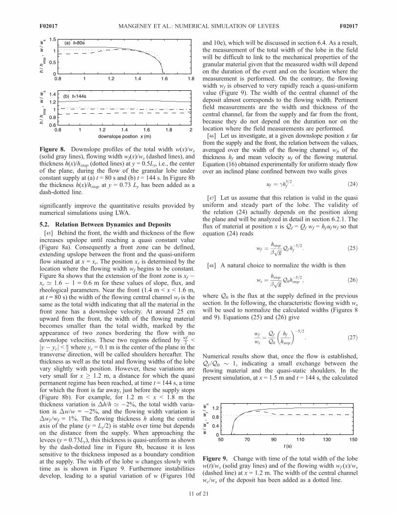
transverse direction, will be called shoulders hereafter. Thethickness as well as the total and flowing widths of the lobevary slightly with position. However, these variations arevery small for x 1.2 m, a distance for which the quasipermanent regime has been reached, at time t = 144 s, a timefor which the front is far away, just before the supply stops(Figure 8b). For example, for 1.2 m < x < 1.8 m thethickness variation is Dh/h ’ �2%, the total width varia-tion is Dw/w = �2%, and the flowing width variation isDwf /wf = 1%. The flowing thickness h along the centralaxis of the plane (y = Ly/2) is stable over time but dependson the distance from the supply. When approaching thelevees (y = 0.73Ly), this thickness is quasi-uniform as shownby the dash-dotted line in Figure 8b, because it is lesssensitive to the thickness imposed as a boundary conditionat the supply. The width of the lobe w changes slowly withtime as is shown in Figure 9. Furthermore instabilitiesdevelop, leading to a spatial variation of w (Figures 10d

and 10e), which will be discussed in section 6.4. As a result,the measurement of the total width of the lobe in the fieldwill be difficult to link to the mechanical properties of thegranular material given that the measured width will dependon the duration of the event and on the location where themeasurement is performed. On the contrary, the flowingwidth wf is observed to very rapidly reach a quasi-uniformvalue (Figure 9). The width of the central channel of thedeposit almost corresponds to the flowing width. Pertinentfield measurements are the width and thickness of thecentral channel, far from the supply and far from the front,because they do not depend on the duration nor on thelocation where the field measurements are performed.[46] Let us investigate, at a given downslope position x far

from the supply and the front, the relation between the values,averaged over the width of the flowing channel wf, of thethickness hf and mean velocity uf of the flowing material.Equation (16) obtained experimentally for uniform steady flowover an inclined plane confined between two walls gives

uf ¼ gh3=2f : ð24Þ

[47] Let us assume that this relation is valid in the quasiuniform and steady part of the lobe. The validity ofthe relation (24) actually depends on the position alongthe plane and will be analyzed in detail in section 6.2.1. Theflux of material at position x is Qf = Qf wf = hf uf wf so thatequation (24) reads

wf ¼hstop

bffiffiffig

p Qf h�5=2f : ð25Þ

[48] A natural choice to normalize the width is then

ws ¼hstop

bffiffiffig

p Q0h�5=2stop ; ð26Þ

where Q0 is the flux at the supply defined in the previoussection. In the following, the characteristic flowing width ws

will be used to normalize the calculated widths (Figures 8and 9). Equations (25) and (26) give

wf

ws

¼ Qf

Q0

hf

hstop

� �5=2

: ð27Þ

Numerical results show that, once the flow is established,Qf /Q0 � 1, indicating a small exchange between theflowing material and the quasi-static shoulders. In thepresent simulation, at x = 1.5 m and t = 144 s, the calculated

Figure 8. Downslope profiles of the total width w(x)/ws

(solid gray lines), flowing width wf(x)/ws (dashed lines), andthickness h(x)/hstop (dotted lines) at y = 0.5Ly, i.e., the centerof the plane, during the flow of the granular lobe underconstant supply at (a) t = 80 s and (b) t = 144 s. In Figure 8bthe thickness h(x)/hstop at y = 0.73 Ly has been added as adash-dotted line.

Figure 9. Change with time of the total width of the lobew(t)/ws (solid gray lines) and of the flowing width wf (x)/ws

(dashed line) at x = 1.2 m. The width of the central channelwc/ws of the deposit has been added as a dotted line.

F02017 MANGENEY ET AL.: NUMERICAL SIMULATION OF LEVEES

11 of 21

F02017

normalized flowing width is wf/ws = 0.90 and the maximumnormalized thickness is hf/hstop = 1.03 so that (hf/hstop)

�5/2 =0.93. The relation

wf

ws

¼ hf

hstop

� �5=2

ð28Þ

would therefore appear hold numerically. The numericalvalues suggest that the flux Qf is slightly smaller than Q0,indicating a nonzero contribution of the transverse velocityto the total flux.[49] Furthermore, the width of the central channel of the

deposit wc is almost equal to wf as shown in Figure 9. As aresult, provided (24) holds for the field granular materialand relation wf (Q0) is defined numerically or experimen-tally (or if ws is known), and provided hstop is known, themeasurement of wc in the field will provide a first-orderestimation of the flowing thickness h and of the velocity uduring emplacement via relations (28) and (24). A moreprecise investigation of the flow and deposit, especiallyconcerning the validity of equation (24), will be presentedin section 6.

5.3. Draining Phase

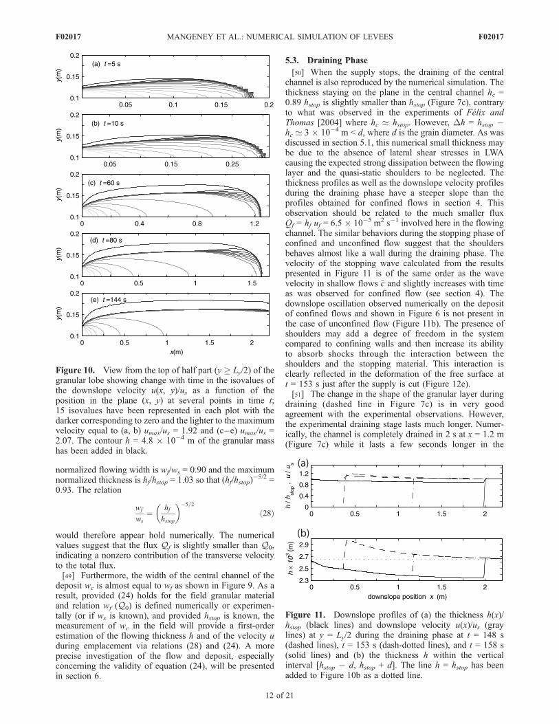
[50] When the supply stops, the draining of the centralchannel is also reproduced by the numerical simulation. Thethickness staying on the plane in the central channel hc =0.89 hstop is slightly smaller than hstop (Figure 7c), contraryto what was observed in the experiments of Felix andThomas [2004] where hc ’ hstop. However, Dh = hstop �hc ’ 3 � 10�4 m < d, where d is the grain diameter. As wasdiscussed in section 5.1, this numerical small thickness maybe due to the absence of lateral shear stresses in LWAcausing the expected strong dissipation between the flowinglayer and the quasi-static shoulders to be neglected. Thethickness profiles as well as the downslope velocity profilesduring the draining phase have a steeper slope than theprofiles obtained for confined flows in section 4. Thisobservation should be related to the much smaller fluxQf = hf uf = 6.5 � 10�5 m2 s�1 involved here in the flowingchannel. The similar behaviors during the stopping phase ofconfined and unconfined flow suggest that the shouldersbehaves almost like a wall during the draining phase. Thevelocity of the stopping wave calculated from the resultspresented in Figure 11 is of the same order as the wavevelocity in shallow flows ~c and slightly increases with timeas was observed for confined flow (see section 4). Thedownslope oscillation observed numerically on the depositof confined flows and shown in Figure 6 is not present inthe case of unconfined flow (Figure 11b). The presence ofshoulders may add a degree of freedom in the systemcompared to confining walls and then increase its abilityto absorb shocks through the interaction between theshoulders and the stopping material. This interaction isclearly reflected in the deformation of the free surface att = 153 s just after the supply is cut (Figure 12e).[51] The change in the shape of the granular layer during

draining (dashed line in Figure 7c) is in very goodagreement with the experimental observations. However,the experimental draining stage lasts much longer. Numer-ically, the channel is completely drained in 2 s at x = 1.2 m(Figure 7c) while it lasts a few seconds longer in the

Figure 10. View from the top of half part (y Ly/2) of thegranular lobe showing change with time in the isovalues ofthe downslope velocity u(x, y)/us as a function of theposition in the plane (x, y) at several points in time t;15 isovalues have been represented in each plot with thedarker corresponding to zero and the lighter to the maximumvelocity equal to (a, b) umax/us = 1.92 and (c–e) umax/us =2.07. The contour h = 4.8 � 10�4 m of the granular masshas been added in black.

Figure 11. Downslope profiles of (a) the thickness h(x)/hstop (black lines) and downslope velocity u(x)/us (graylines) at y = Ly/2 during the draining phase at t = 148 s(dashed lines), t = 153 s (dash-dotted lines), and t = 158 s(solid lines) and (b) the thickness h within the verticalinterval [hstop � d, hstop + d]. The line h = hstop has beenadded to Figure 10b as a dotted line.

F02017 MANGENEY ET AL.: NUMERICAL SIMULATION OF LEVEES

12 of 21

F02017

experimental case. This observation is very similar to theresult of the comparison between numerical and experi-mental results on the spreading of a granular column over ahorizontal plane [Mangeney-Castelnau et al., 2005]. Thestopping phase was expected to be due to complex verticalpropagation of the interface between static and flowinggrains, which is not considered at all by our model.

6. Dynamics of Unconfined Flow

6.1. Several Flow Structures Within the Lobe

[52] The distribution of velocities makes it possible toshed light on the structure of the flow. From the verybeginning, a front zone appears, creating two zones border-ing the flow with very small downslope velocities. These

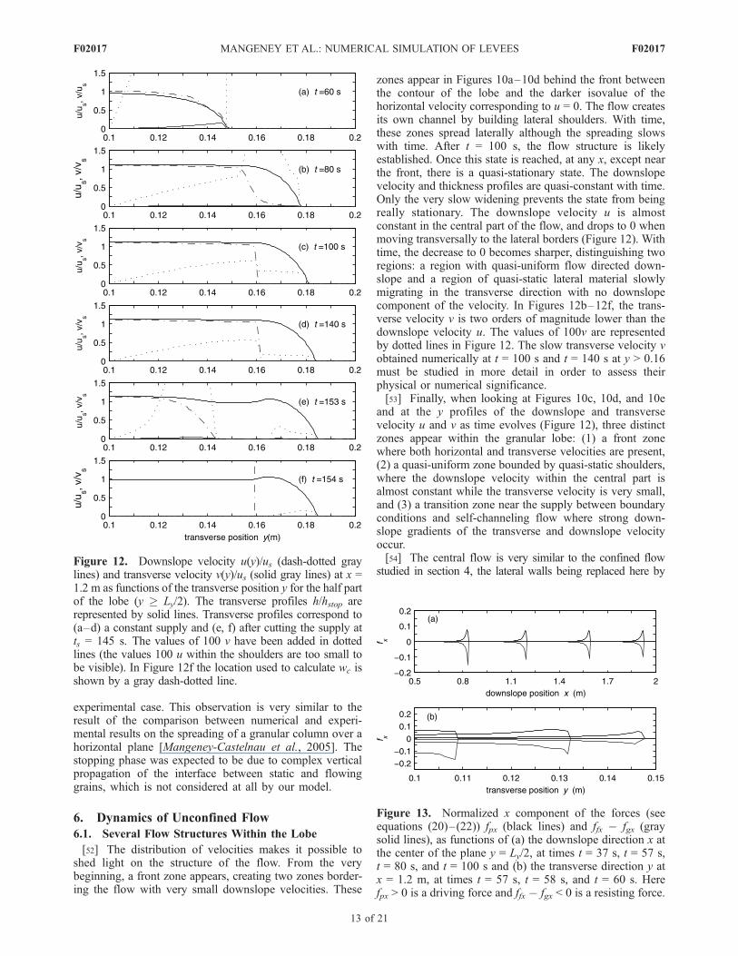
zones appear in Figures 10a–10d behind the front betweenthe contour of the lobe and the darker isovalue of thehorizontal velocity corresponding to u = 0. The flow createsits own channel by building lateral shoulders. With time,these zones spread laterally although the spreading slowswith time. After t = 100 s, the flow structure is likelyestablished. Once this state is reached, at any x, except nearthe front, there is a quasi-stationary state. The downslopevelocity and thickness profiles are quasi-constant with time.Only the very slow widening prevents the state from beingreally stationary. The downslope velocity u is almostconstant in the central part of the flow, and drops to 0 whenmoving transversally to the lateral borders (Figure 12). Withtime, the decrease to 0 becomes sharper, distinguishing tworegions: a region with quasi-uniform flow directed down-slope and a region of quasi-static lateral material slowlymigrating in the transverse direction with no downslopecomponent of the velocity. In Figures 12b–12f, the trans-verse velocity v is two orders of magnitude lower than thedownslope velocity u. The values of 100v are representedby dotted lines in Figure 12. The slow transverse velocity vobtained numerically at t = 100 s and t = 140 s at y > 0.16must be studied in more detail in order to assess theirphysical or numerical significance.[53] Finally, when looking at Figures 10c, 10d, and 10e

and at the y profiles of the downslope and transversevelocity u and v as time evolves (Figure 12), three distinctzones appear within the granular lobe: (1) a front zonewhere both horizontal and transverse velocities are present,(2) a quasi-uniform zone bounded by quasi-static shoulders,where the downslope velocity within the central part isalmost constant while the transverse velocity is very small,and (3) a transition zone near the supply between boundaryconditions and self-channeling flow where strong down-slope gradients of the transverse and downslope velocityoccur.[54] The central flow is very similar to the confined flow

studied in section 4, the lateral walls being replaced here byFigure 12. Downslope velocity u(y)/us (dash-dotted graylines) and transverse velocity v(y)/us (solid gray lines) at x =1.2 m as functions of the transverse position y for the half partof the lobe (y Ly/2). The transverse profiles h/hstop arerepresented by solid lines. Transverse profiles correspond to(a–d) a constant supply and (e, f) after cutting the supply atts = 145 s. The values of 100 v have been added in dottedlines (the values 100 u within the shoulders are too small tobe visible). In Figure 12f the location used to calculate wc isshown by a gray dash-dotted line.

Figure 13. Normalized x component of the forces (seeequations (20)–(22)) fpx (black lines) and ffx � fgx (graysolid lines), as functions of (a) the downslope direction x atthe center of the plane y = Ly/2, at times t = 37 s, t = 57 s,t = 80 s, and t = 100 s and (b) the transverse direction y atx = 1.2 m, at times t = 57 s, t = 58 s, and t = 60 s. Herefpx > 0 is a driving force and ffx � fgx < 0 is a resisting force.

F02017 MANGENEY ET AL.: NUMERICAL SIMULATION OF LEVEES

13 of 21

F02017

quasi-static shoulders. Figure 13 shows the forces acting on thegranular mass during the flow in the x direction as functionsof x (Figure 13a) and as functions of y (Figure 13b). Thepressure force is represented together with the differencebetween the friction force and the force of gravity. Theinertial force is shown to be negligible in Figure 13 exceptat t = 37 s and t = 57 s where the deceleration @u/@t issignificant because of the high resisting force ffx � fgx (grayline) compared to the driving pressure force fpx (black line).As for confined flow, at leading order, in the x direction, thefriction force balances the force of gravity (ffx � fgx = 0)except at the front as shown in Figure 13a where the normof the pressure force increases as does the differencebetween the friction force and the gravity force. Initially,the resisting friction force (ffx � fgx) is higher than the drivingpressure force fpx as is the case at t = 37 s in Figure 13a atthe front. With time, the forces at the front balance each otherin order for the flow to reach a steady state (Figure 13a). Asimilar balance is observed within the granular lobe whenrepresenting the x component of the forces as a function ofthe y direction (Figure 13b). While the dissipation forceis higher than the pressure force within the granular lobe att = 57 s, these forces almost balance each other at t = 60 s(Figure 13b) although the flow just at the lateral margins isnot perfectly solved numerically (see Tai et al. [2002] formore sophisticated numerical treatment of the margins). Inour simple model, the second-order balance between thechange of the friction force and the pressure force is shownto play a key role in the dynamics of the flow, making itpossible to reach a steady state with nonuniform thickness.This balance would certainly change if the disregardedcomponents of the stresses were accounted for.

6.2. Dynamic Path and Flow Law

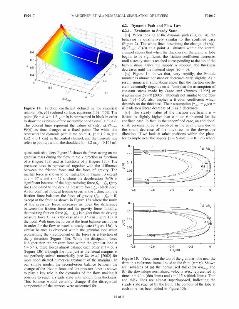
6.2.1. Evolution to Steady State[55] When looking at the dynamic path (Figure 14), the

behavior is qualitatively similar to the confined case(Figure 2). The white lines describing the change of (m(t),h(t)/hstop, Fr(t)) at a point A1 situated within the centralchannel shows that when the thickness of the granular lobebegins to be significant, the friction coefficient decreasesuntil a steady state is reached corresponding to the top of thehatpin shape. Once the supply is stopped, the thicknessdecreases until the material stops (Fr = 0).[56] Figure 14 shows that, very rapidly, the Froude

number is almost constant or decreases very slightly. As aresult, numerical simulations show that the friction coeffi-cient essentially depends on h. Note that the assumption ofconstant stress made by Dade and Huppert [1998] orKelfoun and Druitt [2005], although not similar to the flowlaw (13)–(15), also implies a friction coefficient whichdepends on the thickness. Their assumption jtXZj = mgch =K leads to a linear decrease of m as h decreases.[57] The steady value of the friction coefficient m =

0.4664 is slightly higher than m = tan q obtained for theconfined case. In fact, in the unconfined case, an additionalsmall pressure force is involved in the equilibrium due tothe small decrease of the thickness in the downslopedirection. If we look at other positions within the plane,for example near the supply (x = 5 mm, y = 0.1 m) where

Figure 14. Friction coefficient defined by the empiricalrelation m(h, Fr) (colored surface, equations (13)–(15)). Thepoint (Fr = b, h = 1.2, m = 0) is represented in black in orderto show the extension of the metastable conditions 0 < Fr < b.The colored lines represent the values of (m(t), h(t)/hstop,Fr(t)) as time changes at a fixed point: The white linerepresents the dynamic path at the point A1 (x = 1.2 m, y =Ly/2 = 0.1 cm) in the central channel, and the magenta linerefers to pointA2 within the shoulders (x = 1.2m, y = 0.165m).

Figure 15. View from the top of the granular lobe near thefront in a reference frame linked to the front (x = xf). Shownare isovalues of (a) the normalized thickness h/hstop and(b) the downslope normalized velocity u/us, represented attimes t = 90 s (thin lines) and t = 115 s (thick lines). Thinand thick lines are almost superimposed, indicating thesteady state reached by the front. The contour of the lobe ateach time has been added in Figure 15b.

F02017 MANGENEY ET AL.: NUMERICAL SIMULATION OF LEVEES

14 of 21

F02017

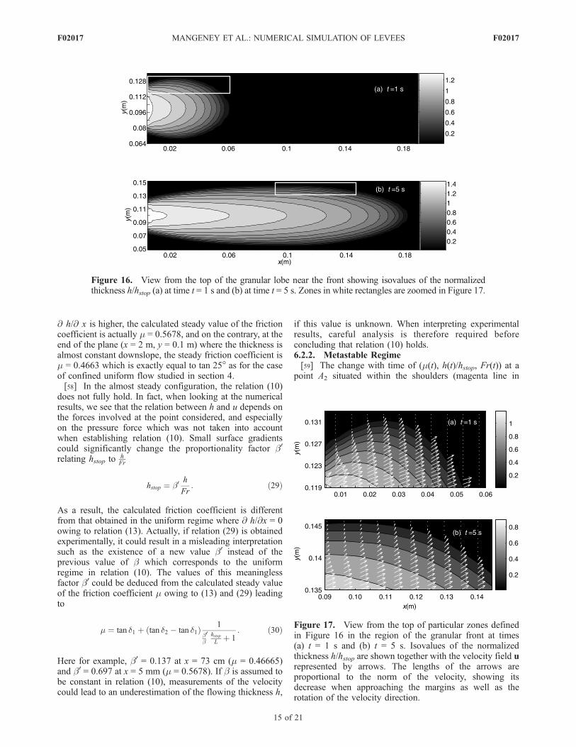
@ h/@ x is higher, the calculated steady value of the frictioncoefficient is actually m = 0.5678, and on the contrary, at theend of the plane (x = 2 m, y = 0.1 m) where the thickness isalmost constant downslope, the steady friction coefficient ism = 0.4663 which is exactly equal to tan 25� as for the caseof confined uniform flow studied in section 4.[58] In the almost steady configuration, the relation (10)

does not fully hold. In fact, when looking at the numericalresults, we see that the relation between h and u depends onthe forces involved at the point considered, and especiallyon the pressure force which was not taken into accountwhen establishing relation (10). Small surface gradientscould significantly change the proportionality factor b0

relating hstop tohFr

hstop ¼ b0 h

Fr: ð29Þ

As a result, the calculated friction coefficient is differentfrom that obtained in the uniform regime where @ h/@x = 0owing to relation (13). Actually, if relation (29) is obtainedexperimentally, it could result in a misleading interpretationsuch as the existence of a new value b0 instead of theprevious value of b which corresponds to the uniformregime in relation (10). The values of this meaninglessfactor b0 could be deduced from the calculated steady valueof the friction coefficient m owing to (13) and (29) leadingto

m ¼ tan d1 þ tan d2 � tan d1ð Þ 1

bb0 hstop

Lþ 1

: ð30Þ

Here for example, b0 = 0.137 at x = 73 cm (m = 0.46665)and b0 = 0.697 at x = 5 mm (m = 0.5678). If b is assumed tobe constant in relation (10), measurements of the velocitycould lead to an underestimation of the flowing thickness h,

if this value is unknown. When interpreting experimentalresults, careful analysis is therefore required beforeconcluding that relation (10) holds.6.2.2. Metastable Regime[59] The change with time of (m(t), h(t)/hstop, Fr(t)) at a

point A2 situated within the shoulders (magenta line in

Figure 16. View from the top of the granular lobe near the front showing isovalues of the normalizedthickness h/hstop (a) at time t = 1 s and (b) at time t = 5 s. Zones in white rectangles are zoomed in Figure 17.

Figure 17. View from the top of particular zones definedin Figure 16 in the region of the granular front at times(a) t = 1 s and (b) t = 5 s. Isovalues of the normalizedthickness h/hstop are shown together with the velocity field urepresented by arrows. The lengths of the arrows areproportional to the norm of the velocity, showing itsdecrease when approaching the margins as well as therotation of the velocity direction.

F02017 MANGENEY ET AL.: NUMERICAL SIMULATION OF LEVEES

15 of 21

F02017

Figure 14) is quite different from that at a point A1 situatedwithin the central channel (white line Figure 14). At thepoint A1, Fr > b always holds. On the other hand, thedynamic path of point A2 (x = 1.2 m, y = 0.165 m) showsnaturally that flow within the levees is always in themetastable regime 0 < Fr < b. Note that this part of theflow law has been determined ad hoc. The shape of the flowlaw in that regime will certainly greatly change the behaviorand shape of the shoulders and levees. However, thedynamic path of point A2 shows that the granular materialnever stops as long as the supply is maintained, as isobserved experimentally [Deboeuf et al., 2006]. This sug-gests that the use of two friction angles, namely a static anda dynamic friction angle, is not necessary to explain theformation of self-channelling flows.[60] The question is why and how this nearly steady self-

channeling flow has been created.

6.3. Creation of the Shoulders Behind the Front

[61] After a certain time (t > 60 s in Figure 10), thestructure of the front zone is clearly different from that ofthe flow behind. The front moves with a constant velocityafter about 60 s when it is located at x 1.3 m. The shapeof the front and the velocity field within the front zonebecomes also constant after around t = 90 s. Figure 15represents a view from the top of the granular lobe. Theisovalues of the normalized thickness (Figure 15a) anddownslope velocity (Figure 15b) in a reference frame linkedto the moving front at t = 90 s (thin lines) and t = 115 s(thick lines) shows that these isovalues, at the differenttimes, are superimposed, reflecting the constant shape andvelocity within the front zone in the reference frame movingwith the front. With time, the front follows its own dynamics.Behind the front, quasi-uniform flow, slightly influenced bythe supply, is established.[62] The shape of the front seems to be responsible for the

selected width of the granular lobe. The creation of should-ers at the rear of the front results from a strong rotation ofthe velocity as shown in Figures 16 and 17 representing twozones behind the front (white rectangles in Figure 16) onwhich it was zoomed in (Figure 17). At the very beginning,at t = 1 s and t = 5 s the velocity at the front is almostconstant and mainly directed downslope (Figure 17). Whenmoving upward from the front, at a given x position thevelocity decreases transversally when approaching the lat-

eral borders and switches from the downslope x directiontoward the transverse y direction (Figure 17). This rotationis also observed at t > 90 s when the front has beenestablished,[63] What makes the velocity decrease and rotate when

approaching the lateral border of the lobe? In the vicinity ofthe front, at t = 57 s, the forces acting in the y direction arealmost zero so that the velocity is mainly directed downslope.Figure 13b shows that the x component of the pressure forcefpx is almost constant transversally at t = 57 s. The force ofgravity is obviously also constant in the x direction. Onthe other hand, the friction is higher when approachingthe shoulders because of small thickness. As a result, thedownslope velocity u decreases when approachingthe lateral border of the lobe. Upward from the front(at t = 58 s in Figure 13b), but still in the front zone, thesame trend can be observed but the x pressure force fpx alsoincreases transversally because of the shape of the front.However, the effect of increasing friction overweighs thedriving effect of the pressure force and the balance of forcesalso leads to a deceleration of the downslope velocity whenapproaching the borders. Obviously, the y component of thefriction force ffy also increases because of small thicknesswhen approaching the borders (Figure 18). The y compo-nent of the gravity force fgy is equal to zero, inertia isnegligible and the driving force is only the pressureforce (black lines in Figure 18). As already observed in thex direction, the increase of dissipation due to frictionoverweighs the increase of driving effects due to surfacegradient @h/@y when approaching the lateral margins andthe transverse velocity decreases (@v/@t < 0). However, thedeceleration in the transverse direction is much smaller thanthe deceleration in the downslope direction because of thehigher driving force fpy than that in the x direction (j@h/@yj >j@h/@xj) near the margins. The total velocity thereforerotates toward the transverse direction and decreases withtime when approaching the lateral borders of the flow(Figure 17). In our simple model, the increase of the frictionwith decreasing thickness may then be the process respon-sible for the creation of shoulders bordering the flow. Thecomplex competition between the pressure force and thefriction when the thickness decreases seems to be a keymechanism controlling the dynamics of the front.[64] However, would it really be necessary to include

variable bed friction to produce the force competition thatcreates lateral levees if the disregarded components of thestress tensor were introduced in the model? In fact, at leastin the SH-type approach, taking into account the anisotropyof normal stresses would add a multiplying coefficient k inthe h gradient term that depends on the sign of the spacegradient of the velocity field. On the other hand, followingthe approach proposed by Iverson and Denlinger [2001],the shear stresses on planes normal to the bed wouldintroduce an additional term related to the y derivative ofthe thickness h in the x momentum equation and anadditional term related to the x derivative of the thicknessh in the y momentum equation. These terms would com-pletely change the balance of forces. In the case of the SHtheory, the creation of quasi-static zones could be explainedin a different way. In fact, the equilibrium in the y directionbehind the front involves a driving force related to the

Figure 18. Normalized y components of the forces (seeequations (20)–(22)): fpy (black solid lines) and ffy (graysolid lines) as functions of the transverse direction y at x =1.2 m and at times t = 58 s, t = 62 s, and t = 66 s. Here fpy > 0 isa driving force and ffy < 0 is a resisting force. Note that they component of the gravity fgy is equal to zero.

F02017 MANGENEY ET AL.: NUMERICAL SIMULATION OF LEVEES

16 of 21

F02017

h gradient in the y direction (pressure force), a lateraldissipation force related to the shear stress tXY involvingthe h gradient in the x direction and the so-called frictionforce. When moving from the center (y = 0) to the lateralborder (y = w/2) at a given position x behind the front, thepressure force increases because of decreasing thickness,the friction force is constant because the friction coefficientm is constant, and the lateral dissipation force increasesbecause @ h/@x decreases behind the front when movingtoward the lateral borders. This analysis suggest a possiblerelation between the m parameterization and the neglectingof stresses on planes normal to the bed.

6.4. Instabilities

[65] Instabilities are observed near the supply as shown inFigure 10e. Instabilities in the lateral part of unconfinedflow have also been observed in the experiments of Deboeuf[2005]. Note that this phenomenon was obtained numeri-cally using a totally different code based on a kineticscheme and finite volume elements with an unstructuredgrid as described by Mangeney-Castelnau et al. [2003].However, more investigations must be carried out in orderto be sure that these instabilities are not of a numericalnature. Some oscillations are also observed near the frontbut seem to be related to the discretization.[66] The region near the supply is subjected to strong

gradients of the velocity field due to the transition betweenboundary conditions and the developed flow along theplane. After a few tens of seconds, near the supply, thewidth of the lobe increases regularly until x ’ 20 cm andstabilizes for larger values of x. An instability occurs at thistransition. One explanation could be that the expansion ofthe granular mass near the supply is blocked by quasi-staticshoulders and the material is only allowed to flow in thedownslope direction. The change of direction from expan-sion to downslope motion may be at the origin of theinitiation of the instability observed in this region. Instabil-ity can also be observed on the dynamic path of the pointssituated within the shoulders (Figure 14). As the thicknessof the shoulders increases after the front has passed thefriction decreases while the Froude number oscillates.

7. Conclusion

[67] It has been shown here that numerical simulationusing the Saint Venant approach with the empirical variablefriction law proposed by Pouliquen and Forterre [2002]makes it possible to simulate the complex behavior ofunconfined flow. The creation of a channel with a givenwidth as well as the separation of the flow between an innerquasi-steady regime in the downslope direction together withquasi-static borders is surprisingly well reproduced. Themajor achievement of these simulations has been to showthat neither mixture concepts nor polydispersity are needed toexplain self-channeling flows and levee formation.[68] The simulation have been performed using a param-

eterization of the coefficient of friction that depends on thethickness and the Froude number of the flow. The model isbased on strong assumptions such as the isotropy of normalstresses and the neglecting of shear stresses on planesnormal to the bed. These assumptions are expected to affectthe interpretation of the results in the case studied here

where quasi-static zones develop near the lateral marginsand where h gradients can be large. In particular, theabsence of lateral dissipation between the flowing massand the quasi-static shoulders likely leads to underestima-tion of the flowing thickness and the thickness of thedeposit in the central channel. Furthermore, Pouliquenand Forterre’s [2002] empirical flow rule is obviouslyoversimplified to describe the behavior of the complexgeological materials involved in natural avalanches.[69] Numerical results provide a possible explanation of

the self-channeling process indicating that the shoulders arecreated behind the front. The fact that the front reaches asteady velocity and shape along the plane seems to beresponsible of the width chosen by the flow. In the simplifiedmodel used here, the formation of shoulders channeling theflow has been shown to result from the balance between afriction force with a friction coefficient depending on thethickness of the flow and the driving forces due to gravity andsurface slope. The competition between these forces leads torotation of the velocity vector from the downslope directionwithin the central channel to the transverse direction whenapproaching the lateral border of the flow. The complexcompetition between the pressure force and the friction whenthe thickness decreases seems to be a key mechanismcontrolling the dynamics of the front. The balance of forceswould be different if stresses on planes normal to the bedwere taken into account. In that case, the increasing dissipa-tion near the lateral borders behind the front would beexpected to be due to the increasing downslope gradient ofthe thickness whenmoving from the center of the lobe towardthe lateral margins. Simulation of self-channelling flows andanalysis of the balance of forces using more sophisticatedmodels such as the one proposed by Denlinger and Iverson[2004] would provide insight into the role of the differentcomponents of the stress tensor in the creation of quasi-staticzones. Furthermore, it could be a way to understand the basisof the m parameterization.[70] The steady regime obtained in the central channel

appears to be very similar to that observed on uniformlaterally confined flows. The calculated flow within thecentral channel almost reaches a steady state with a constantvalue of the thickness and velocity at a given position. Wehave investigated the variation of the friction coefficientduring the flow. The nonuniformity in space involvingsurface gradients locally modifies the steady coefficient offriction calculated by the numerical model, which appears tobe slightly different from the case of steady uniformconfined flow (m = tan q). The dependence on the velocityof the friction coefficient appears to be weak. In fact, oncethe flow has developed, the Froude number is almostconstant because the velocity varies like the wave velocityin shallow flow. The metastable regime is thoroughlyinvestigated by the flow near the developing quasi-staticmargins. The accurate description of this regime is thereforeessential when modeling the dynamics of these zones andthe shape of the levees. However, in the case of our model,the granular material never stops as long as the supply ismaintained as observed experimentally [Deboeuf et al.,2006]. This suggests that the use of two friction angles,namely a static and a dynamic friction angle, is notnecessary to explain self-channelling flows.

F02017 MANGENEY ET AL.: NUMERICAL SIMULATION OF LEVEES

17 of 21

F02017

[71] The width of the flowing channel wf has been provedto be almost constant in time and space. The width of thecentral channel on the deposit wc almost corresponds to wf

and therefore provides a pertinent parameter for fieldmeasurements. Furthermore, the thickness in the centralchannel of the deposit hc almost corresponds to hstop, aparameter containing information on the mechanical prop-erties of the granular mass. If the relation between theflowing width and the initial flux wf(Q0) has been deter-mined experimentally or numerically, the measurements onthe field of the two parameters (hc, wc) would allowestimation of the thickness and velocity of the flow duringemplacement. For pyroclastic flows, it would allow estima-tion of the flux of material emitted by the volcano. Thedetailed study of geomorphologic features observed ondeposits of gravitational flows has been shown to providea useful tool for the comparison of model and fieldobservations and sheds new light on the flow law governingthe motion of these complex granular flows.

Appendix A

[72] This appendix presents the new model used, whichtakes into account the curvature tensor

H ¼ c3@2b@x2

@2b@x@y

@2b@x@y

@2b@y2

!ðA1Þ

with all its components [Bouchut and Westdickenberg,2004], although these components are equal to zero in thesimple case studied here. In one dimension, our formulationcan be reduced to the equations developed in former studies.The flow is described by

h t; xð Þ 0; u0 t; xð Þ 2 R2; ðA2Þ

where h is the thickness of the material layer in the directionnormal to the topography, and u0 = (u, ut) (where thesubscript t stands for transverse) is a parameterization of thevelocity. This parameterization has been defined in order tosimplify the equations when a 1-D topography b = b(x) isconsidered. The real 3-D material velocity has horizontal/vertical components

u!¼ cu0; s � vu0ð Þ: ðA3Þ

This physical velocity is tangent to the topography, u! � u! =0, as would be expected for shallow flows and can beexpressed as a 2-D vector u = (u, v) in the (X, Y) plane(Figure 1). In one dimension, u0 is actually the real scalarvelocity u in the plane tangent to the topography. In the casesimulated below dealing with the flow over an inclinedplane with slope in the x direction, the real physical velocityu has coordinates in the tangent plane given by

u; vð Þ ¼ u; cutð Þ: ðA4Þ

[73] In the horizontal Cartesian coordinate formulation,the model can be expressed as (see (2.54)–(2.55) in workby Bouchut and Westdickenberg [2004])

@t h=cð Þ þ rx � hu0ð Þ ¼ 0 ðA5Þ

@tu0 þ cu0 � rxu

0 þ 1

cId� sstð Þrx g hcþ bð Þð Þ ¼

� 1

cu0

tHu0 �

sþ 1

cstHu0ð Þu0 � gmcu0ffiffiffiffiffiffiffiffiffiffiffiffiffiffiffiffiffiffiffiffiffiffiffiffiffiffiffiffiffiffiffiffiffiffiffiffi

c2jju0jj2 þ s � u0ð Þ2q

� 1þ u0tHu0

gc

� þ;

ðA6Þ

where rx is the gradient vector in the horizontal x, y planeand g acceleration due to gravity. The subscript + standsfor the positive part, x+ = max(0, x). The system (A5) and(A6), is obtained using a trick that consists of performingan asymptotic analysis of the free surface incompressibleNavier-Stokes equations although the final model is notbased on the Navier-Stokes equations; that is, viscouseffects are not accounted for. Equations (A5) and (A6) areobtained by this asymptotic analysis up to errors O(�3)and O(�2) respectively for mass and velocity equations, asthe aspect ratio � approaches 0. It is obtained by assumingthat the viscosity v = O(�2), the Coulomb bottom frictioncoefficient m = O(v/�), and the curvature H = O(�)[Bouchut and Westdickenberg, 2004]. The model isinvariant with respect to rotation, admits a conservativeenergy equation and preserves the steady state of a lake atrest. For flow over an inclined plane, the case consideredhere, the equations can be reduced to (3) and (4).

Appendix B

[74] The numerical method in the one-dimensional casehas been discussed by Mangeney-Castelnau et al. [2005],and we will review only the formulas here before extendingthe method to two dimensions.

B1. Saint Venant Problem With Topography andFriction in One Dimension

[75] Let us first describe the 1-D scheme in order topresent the basic principles of the numerical method. Theone-dimensional Saint Venant system with topography andfriction is expressed as

@thþ @x huð Þ ¼ 0;

@t huð Þ þ @x hu2 þ gh2=2ð Þ þ hgbx ¼ hf ;

(ðB1Þ

where b(x) represents topography and bx the derivative of bas a function of x, and where the friction force f = f(t, x)must satisfy

j f t; xð Þj � gm;

u t; xð Þ 6¼ 0 ) f t; xð Þ ¼ �gmu t; xð Þju t; xð Þj :

8<: ðB2Þ

F02017 MANGENEY ET AL.: NUMERICAL SIMULATION OF LEVEES

18 of 21

F02017

The 1-D version of the system (2)–(7) is of the form (A7)–(A8) after a slight change of notation (from (2)–(4) and (7),define x0 = x/c, g0 = gc, b0 = b/c, and use these new variablesin order to identify the system with (A7)–(A8)). In thissystem the steady states at rest play a crucial role and aregiven by u = 0, f = @x(gh + gb), or equivalently,

u ¼ 0 and j@x hþ bð Þj � m: ðB3Þ

We are interested in using well-balanced schemes, i.e.,schemes that preserve steady states at the discrete level. Theapparent topography approach considers the source term asa topography by defining g@x~b = �f. Consider a 1-D meshmade of cells of size Dx. The cells are defined by

Ci ¼ �xi�1=2; xiþ1=2½ ðB4Þ

of length Dxi = xi+1/2 � xi�1/2. The cell centers are denotedxi = (xi+1/2 + xi�1/2)/2. We consider a time stepDt and definethe discrete times by tn = nDt, with n 2 N. According toMangeney-Castelnau et al. [2005], this leads to thefollowing formulas,

Unþ1i � Un

i þDt

DxiFiþ1=2� � Fi�1=2þ �

¼ 0; ðB5Þ

where Uin

Uni ’

1

Dxi

ZCi

U tn; xð Þdx ðB6Þ

is an approximation of the average of the exact solution attime tn

U ¼ h

hu

� ðB7Þ

over the cell Ci. The left/right numerical fluxes arecomputed as

Fiþ1=2� ¼ Fl Ui;Uiþ1;Dbiþ1=2 þD~bniþ1=2

� �Fiþ1=2þ ¼ Fr Ui;Uiþ1;Dbiþ1=2 þD~bn

iþ1=2

� �;

ðB8Þ

with Dbi+1/2 = bi+1 � bi, and

gD~bniþ1=2 ¼ �f niþ1=2Dx: ðB9Þ

[76] The numerical fluxes Fl and Fr are derived by thehydrostatic reconstruction method [Audusse et al., 2004],and have the following form:

Fl Ul;Ur;Dbð Þ ¼ F U*l ;U*r

� �þ g

2h2l �

g

2h2l*

00@ 1A

Fr Ul;Ur;Dbð Þ ¼ F U*l ;U*r

� �þ g

2h2r �

g

2h2r*

00@ 1A;

ðB10Þ

where Ul* = (hl*

, hl*ul), Ur

* = (hr*, hr*

ur), and

hl* ¼ max 0; hl �max 0;Dbð Þð Þ

hr* ¼ max 0; hr �max 0;�Dbð Þð Þ: ðB11Þ

[77] Here F is any entropy satisfying consistent numer-ical flux for the homogeneous problem (i.e., without topog-raphy and friction), that is capable of dealing with drystates. We use a relaxation solver described by Bouchut[2004], but other choices give similar results.[78] Then, if f i+1/2

n is a consistent value for the friction, itis easy to see that our scheme is consistent with (A7) andwell-balanced since it preserves the discrete steady statessatisfying ui = ui+1 = 0 and ghi+1 � ghi + gDbi+1/2 = fi+1/2Dx.The scheme also conserves mass, is capable of computing drybed states and satisfies a discrete entropy inequality. For thecomputation of f i+1/2

n , a good choice is

f niþ1=2 ¼ �g projm

hi � hiþ1 �Dbiþ1=2

Dxþuiþ1=2

gDt

� ; ðB12Þ

where

projm

Xð Þ ¼X if jX j � m;

mX

jX j if jX j > m; :

8><>: ðB13Þ

and, for example,

uiþ1=2 ¼hiui þ hiþ1uiþ1

hi þ hiþ1

: ðB14Þ

This gives a well-balanced scheme, in the sense that datasatisfying

ui ¼ 0 and jhi � hiþ1 �Dbiþ1=2j � mDx ðB15Þ

are preserved exactly. For higher precision, a better choice isto replace (B12) by

f niþ1=2 ¼ �g Projm

hi � hiþ1 �Dbiþ1=2

Dx;uiþ1=2

gDt

� ; ðB16Þ

where

Projm

X ; Yð Þ ¼ projm

projm

Xð Þ þ 2

1þmax 1;�X � Y=mjY jð ÞY !

:

ðB17Þ

For models where m = m(h, u), the definitions can easily beextended using local values mi+1/2 in (B12) or (B17). Thenumerical processing of the friction presented above leads toa regularization of the friction for small velocities. Actually,in the case of small velocity, equations (B12) or (B17)compute a friction force directed opposite to the sum of h andb gradients (i.e., the gradient of pressure added to the force ofgravity) and set its norm equal to the norm of this sum.

F02017 MANGENEY ET AL.: NUMERICAL SIMULATION OF LEVEES

19 of 21

F02017

B2. Two-Dimensional Scheme

[79] The two-dimensional Saint Venant system withtopography and friction is written

@thþ @x huð Þ þ @y hvð Þ ¼ 0

@t huð Þ þ @x hu2 þ gh2=2ð Þ þ @y huvð Þ þ hg@xb ¼ hfx

@t hvð Þ þ @x huvð Þ þ @y hv2 þ gh2=2ð Þ þ hg@yb ¼ hfy;

8><>: ðB18Þ

where b(x, y) represents the 2-D topography and where thefriction force f(t, x, y) = (fx, fy) must satisfy

jjf t; x; yð Þjj � gm

u t; x; yð Þ 6¼ 0 ) f t; x; yð Þ ¼ �gmu t; x; yð Þ

jju t; x; yð Þjj ;

8<: ðB19Þ

with u = (u, v). As explained in section 9.1 The system (2)–(4) and (7) is of the form (B18)–(B19) after a slight changeof notation. As in the 1-D case, we will describe the schemefor (B18)–(B19). In this system the steady states at rest aregiven by u = 0, f = rx(gh + gb), or, equivalently,

u ¼ 0 and jjrx hþ bð Þjj � m: ðB20Þ

[80] As usual, the 2-D finite volume method is performedusing the 1-D scheme interface by interface. Note that the1-D system corresponding to (B18) is (A7) with theaddition of the advection equation @t(hv) + @x(huv) = 0.[81] Consider a two-dimensional mesh made of rectangles

of sizesDx,Dy. The rectangles shall be defined by subscripts(i, j), and the interfaces between two adjacent rectangles by(i + 1/2, j) and (i, j + 1/2). The approximate value of

U ¼h

hu

hv

0@ 1A ðB21Þ

over the rectangle (i, j) is denoted by Uijn, where n refers to

the time level (not always indicated here for simplicity). Thesolution U and the numerical fluxes F are 3-D vectors butwill be written here in bold symbols for the sake ofsimplicity. Then, the two-dimensional scheme is written

Unþ1ij � Un

ij þDt

DxFiþ1=2�;j � Fi�1=2þ;j

�þDt

DyFi;jþ1=2� � Fi;j�1=2þ �

¼ 0;ðB22Þ

where the interface fluxes are computed via

Fiþ1=2�;j ¼ Fl=r Uij;Uiþ1;j;Dbiþ1=2;j þD~biþ1=2;j

�Fi;jþ1=2� ¼ bFl=r

bUij; bUi;jþ1;Dbi;jþ1=2 þD~bi;jþ1=2

� �:

ðB23Þ

[82] In (B23), we denote Dbi+1/2,j = bi+1,j � bij,Dbi,j+1/2 =bi,j+1 � bij, bU = (h, hv, hu) if U = (h, hu, hv). The 2-Dnumerical fluxes are defined as follows if Ul = (hl, hlul, hlvl)and Ur = (hr, hrur, hrvr),

Fl=r Ul;Ur;Dbð Þ ¼ Fl=r hl; hlul; hr; hrur;Dbð Þ

� Fhl=r hl; hlul; hr; hrur;Dbð Þv

*Þ; ðB24Þ

where Fl/r are the one-dimensional fluxes (B10)–(B11), thepower h refers to the first component (note that Fl

h = Frh),

and

v* ¼vl if Fh

l=r hl ; hlul; hr; hrur;Dbð Þ 0

vr if Fhl=r hl; hlul ; hr; hrur;Dbð Þ � 0:

(ðB25Þ

The apparent topography terms are related to the frictionforces by

gD~biþ1=2;j ¼ � fiþ1=2;j

�xDx

gD~bi;jþ1=2 ¼ � fi;jþ1=2

�yDy;

ðB26Þ

where the indices x and y relate to the x and y componentsrespectively. According to the multidimensional finitevolume formulation of well-balanced schemes of Bouchut[2004], note that the x fluxes in (B22) involve the xcomponent of f, while the y fluxes involve the y componentof f. Finally, the friction terms are computed by theprojections

f iþ1=2;j ¼ �g Projm

hij � hiþ1;j �Dbiþ1=2;j

Dx; 0

� ��uiþ1=2;j

gDt

f i;jþ1=2 ¼ �g Proj

m0;hij � hi;jþ1 �Dbi;jþ1=2

Dy

� ��ui;jþ1=2

gDt

;

ðB27Þ

where Proj is still defined by (B23) but with X, Y two-dimensional vectors, and

uiþ1=2;j ¼hijuij þ hiþ1;juiþ1;j

hij þ hiþ1;j

ui;jþ1=2 ¼hijuij þ hi;jþ1ui;jþ1

hij þ hi;jþ1

:

ðB28Þ

[83] Acknowledgments. We thank R. Iverson and K. Hutter for theirinsight and comments that have greatly improved this paper. We thankB. Perthame for fruitful discussions. We thank the members of the GdRMiDi for interesting remarks. This work was supported by the ActionConcertee Incitative Nouvelles Interfaces des Mathematiques (CNRS), theAction Concertee Incitative Jeunes Chercheurs (CNRS), and the ACI Aleaset Changements Globaux (CNRS). This is contribution IPGP 2176.

ReferencesAudusse, E., F. Bouchut, M. O. Bristeau, R. Klein, and B. Perthame (2004),A fast and stable well-balanced scheme with hydrostatic reconstructionfor shallow water flows, SIAM J. Sci. Comput., 25, 2050–2065.

Bouchut, F. (2004), Nonlinear Stability of Finite Volume Methods forHyperbolic Conservation Laws, and Well-Balanced Schemes for Sources,Frontiers Math. Ser., Springer, New York.

Bouchut, F., and M. Westdickenberg (2004), Gravity driven shallow watermodels for arbitrary topography Commun, Math. Sci., 2, 359–389.

Calder, E. S., R. S. J. Sparks, and M. C. Gardeweg (2000), Erosion, trans-port and segregation of pumice and lithic clasts in pyroclastic flowsinferred from ignimbrite at Lascar Volcano, Chile, J. Volcanol. Geotherm.Res., 104, 201–235.

Da Cruz, F. (2004), Ecoulement de grains secs: Frottement et blocage,Ph.D. thesis, Ecole Natl. des Ponts et Chaussees, Marne la Vallee, France.

Dade, W. B., and H. E. Huppert (1998), Long runout rockfalls, Geology, 26,803–806.

Daerr, A., and S. Douady (1999), Two types of avalanche behaviour ingranular media, Nature, 399, 241–243.

Deboeuf, S. (2005), Transition et coexistence solide-liquide dans les mate-riaux granulaires, Ph.D. thesis, Inst. de Phys. du Globe de Paris, Paris,France.

F02017 MANGENEY ET AL.: NUMERICAL SIMULATION OF LEVEES

20 of 21

F02017

Deboeuf, S., O. Dauchot, L. Staron, A. Mangeney, and J. P. Vilotte (2005a),Memory of the unjamming transition during cyclic tiltings of a granularpile, Phys. Rev. E, 72, 051305.

Deboeuf, S., O. Dauchot, L. Staron, J. P. Vilotte, and A. Mangeney (2005b),Evolution of the contact network during tilting cycles of a granular pileunder gravity, in Powders and Grains, edited by R. Garcıa-Rojo, H. J.Herrmann, and S. McNamara, pp. 105–108, A. A., Balkema, Brookfield, Vt.

Deboeuf, S., E. Lajeunesse, O. Dauchot, and B. Andreotti (2006), Flowrule, self-channelization and levees in unconfined granular flows Phys,Rev. E, 97, 158303.

Denlinger, R. P., and R. M. Iverson (2001), Flow of variably fluidizedgranular masses across three-dimensional terrain: 2. Numerical predic-tions and experimental tests, J. Geophys. Res., 106, 553–566.

Denlinger, R. P., and R. M. Iverson (2004), Granular avalanches acrossirregular three-dimensional terrain: 1. Theory and computation, J. Geophys.Res., 109, F01014, doi:10.1029/2003JF000085.

Douady, S., B. Andreotti, and A. Daerr (1999), On granular surface flowequations, Eur. Phys. J. B, 11, 131–142.

Ertas, D., G. S. Grest, T. C. Halsey, D. Levine, and L. Silbert (2001),Gravity-driven dense granular flows, Europhys. Lett., 56, 214–220.

Felix, G., and N. Thomas (2004), Relation between dry granular flowregimes and morphology of the deposits: Formation of levees in pyro-clastic deposits, Earth Planet. Sci. Lett., 221, 197–231.

Forterre, Y., and O. Pouliquen (2003), Long-surface-wave instability indense granular flows, J. Fluid Mech., 486, 21–50.

Gray, J. M. N. T., M. Wieland, and K. Hutter (1999), Gravity driven freesurface flow of granular avalanches over complex basal topography,Proc. R. Soc. London, Ser. A, 455, 1841–1874.

Hutter, K., and T. Koch (1991), Motion of a granular avalanche in anexponentially curved chute: Experiments and theoretical predictions, Phi-los. Trans. R. Soc. London, Ser. A, 334, 93–138.

Hutter, K., T. Koch, C. Pluss, and S. B. Savage (1995), The dynamicsof avalanches of granular materials from initiation to run out. part II,Experiments, Acta Mech., 109, 127–165.

Iverson, R. M., and R. P. Denlinger (2001), Flow of variably fluidizedgranular masses across three-dimensional terrain: 1. Coulomb mixturetheory, J. Geophys. Res., 106, 537–552.

Iverson, R. M., and J. Vallance (2001), New views of granular mass flows,Geology, 29, 115–118.

Iverson, R. M., M. Logan, and R. P. Denlinger (2004), Granular avalanchesacross irregular three-dimensional terrain: 2. Experimental tests, J. Geo-phys. Res., 109, F01015, doi:10.1029/2003JF000084.

Jop, P., Y. Forterre, and O. Pouliquen (2005), Crucial role of sidewalls ingranular surface flows: Consequences for the rheology, J. Fluid Mech.,541, 167–192.

Kelfoun, K., and T. H. Druitt (2005), Numerical modeling of the emplace-ment of Socompa rock avalanche, Chile, J. Geophys. Res., 110, B12202,doi:10.1029/2005JB003758.

Klaucke, I., D. G. Masson, N. H. Kenyon, and J. V. Gardner (2004),Sedimentary processes on the lower Monterey Fan Channel and channel-mouth lobe, Mar. Geol., 206, 181–198.

Lucas, A., and A. Mangeney (2007), Mobility and topographic effects forlarge Valles Marineris landslides on Mars, Geophys. Res. Lett.,doi:10.1029/2007GL029835, in press.

Malin, M. C., and K. S. Edgett (2000), Evidence for recent groundwaterseepage and surface runoff on Mars, Science, 228, 2330–2335.

Mangeney-Castelnau, A., J.-P. Vilotte, M. O. Bristeau, B. Perthame,F. Bouchut, C. Simeoni, and S. Yerneni (2003), Numerical modeling ofavalanches based on Saint Venant equations using a kinetic scheme,J. Geophys. Res., 108(B11), 2527, doi:10.1029/2002JB002024.

Mangeney-Castelnau, A., F. Bouchut, J. P. Vilotte, E. Lajeunesse,A. Aubertin, and M. Pirulli (2005), On the use of Saint Venant equationsto simulate the spreading of a granular mass, J. Geophys. Res., 110,B09103, doi:10.1029/2004JB003161.

Mangold, N., F. Costard, and F. Forget (2003), Debris flows over sanddunes on Mars: Evidence for liquid water, J. Geophys. Res., 108(E4),5027, doi:10.1029/2002JE001958.

McDonald, R. R., and R. S. Anderson (1996), Constraints on eolian grainflow dynamics through laboratory experiments on sand slope, J. Sediment.Res., 66, 642–653.

McDougall, S., and O. Hungr (2004), A model for the analysis of rapidlandslide runout motion across three-dimensional terrain, Can. Geotech.J., 41, 1084–1097.

Naaim, M., S. Vial, and R. Couture (1997), Saint Venant approach for rockavalanches modelling, paper presented at the Saint Venant Symposium,Paris, 28–29 Aug.

Nairn, I. A., and S. Self (1978), Explosive eruptions and pyroclastic ava-lanches from Ngauruhoe in February 1975, J. Volcanol. Geotherm. Res.,3, 39–60.

Pastor, M., J. A. Fernandez Merodo, M. Quecedo, M. I. Herreros,E. Gonzales, and P. Mira (2002), Modelling of debris flows and flowslides, Numer. Modell. Geomech., 6, 1213–1232.

Pirulli, M., A. Mangeney, M. O. Bristeau, and C. Scavia (2007), The effectof the Earth pressure coefficients on the runout of granular materials,Environm. Modell. Software, in press.

Pitman, E. B., C. C. Nichita, A. K. Patra, A. C. Bauer, M. Sheridan, andM. Bursik (2003), Computing granular avalanches and landslides, Phys.Fluids, 15, 3638–3646.

Pouliquen, O. (1999), Scaling laws in granular flows down rough inclinedplanes, Phys. Fluids, 11, 542–548.

Pouliquen, O., and Y. Forterre (2002), Friction law for dense granularflows: Application to the motion of a mass down a rough inclined plane,J. Fluid Mech., 453, 133–151.

Quareni, F., A. Tallarico, and M. Dragoni (2004), Modeling of the steady-state temperature field in lava flow leves, J. Volcanol. Geotherm. Res.,132, 241–251.

Roberts, A. W. (1965), An investigation of the gravity flow of noncohesivematerials through discharge chutes, Trans. ASME, 91, 373–381.

Rodriguez-Elizarraras, S., C. Siebe, J. C. Komorowski, J. M. Expindola,and R. Saucedo (1991), Field observations of pristine block and ash flowdeposits emplaced April 16–17, 1991 at Volcan de Colima, Mexico,J. Volcanol. Geotherm. Res., 48, 399–412.

Rowley, P. D., M. A. Kuntz, and N. S. MacLeod (1991), Pyroclastic-flowdeposits, U.S. Geol. Surv. Prof. Pap., 1250, 489–512.

Sakimoto, S. E. H., and T. K. P. Gregg (2001), Channeled flow: Analyticsolutions, laboratory experiments, and applications to lava flows, J. Geophys.Res., 106, 8629–8644.

Saucedo, R., J. L. Macas, M. I. Bursik, J. C. Mora, J. C. Gavilanes, andA. Cortes (2002), Emplacement of pyroclastic flows during the 1998–1999 eruption of Volcan de Colima, Mexico, J. Volcanol. Geotherm. Res.,117, 129–153.

Savage, S. B. (1979), Gravity flow of cohesionless granular materials inchutes and channels, J. Fluid Mech., 92, 53–96.

Savage, S. B., and K. Hutter (1989), The motion of a finite mass of granularmaterial down a rough incline, J. Fluid Mech., 199, 177–215.

Sheridan, M. F., A. J. Stinton, A. Patra, E. B. Pitman, A. Bauer, andX. Nichita (2007), Evaluating TITAN2D mass-flow model using the1963 Little Tahoma Peak avalanches, Mount Rainier, Washington,J. Volcanol. Geotherm. Res., in press.

Sokolovski, V. (1965), Statics of Granular Media, Elsevier, New York.Taberlet, N., P. Richard, A. Vallance, W. Losert, J. M. Pasini, J. T. Jenkins,and R. Delannay (2003), Superstable granular heap in a thin channel,Phys. Rev. Lett., 91, 264301.

Tai, Y. C., S. Noelle, N. Gray, and K. Hutter (2002), Shock capturing andfront tracking methods for granular avalanches, J. Comput. Phys., 175,269–301.

Treiman, A. H., and M. Y. Louge (2004), Martian slope streaks and Gullies:Origins as dry granular flows, Lunar Planet. Sci., (XXXV), abstract 1323.

Ui, T., N. Matsuwo, M. Sumita, and A. Fujinawa (1999), Generation ofblock and ash flows during the 1990–1995 eruption of Unzen volcano,Japan, J. Volcanol. Geotherm. Res., 89, 123–137.

Wilson, L., and J. W. Head (1981), Morphology and rheology of pyroclasticflows and their deposits, and guidelines for future observations, U.S.Geol. Surv. Bull., 1250, 513–524.

Yamamoto, T., S. Takarada, and S. Suto (1993), Pyroclastic flows from the1991 eruption of Unzen volcano, Japan, Bull. Volcanol., 55, 166–175.

�����������������������F. Bouchut, Departement de Mathematique et Applications, Ecole

Normale Superieure, 45 rue d’Ulm, F-75230 Paris cedex 05, France.([email protected])M. O. Bristeau, INRIA, Projet BANG, BP105, F-78153 Le Chesnay

cedex, France. ([email protected])A. Mangeney, Institute for Nonlinear Science, University of California,

San Diego, CMRR Building, 9500 Gilman Drive, La Jolla, CA 92093-0402, USA. ([email protected])N. Thomas, IUSTI, CNRS, 5 rue E. Fermi, Technopole de Chateau-

Gombert, F-13453 Marseille, France. ([email protected])J. P. Vilotte, Equipe de Sismologie, Institut de Physique du Globe de

Paris, 4 place Jussieu, F-75252 Paris cedex 05, France. ([email protected])

F02017 MANGENEY ET AL.: NUMERICAL SIMULATION OF LEVEES

21 of 21

F02017