Numerical Modeling of Earth Dam Breaching by Overtopping André Filipe Paulos Lopes Thesis to obtain the Master of Science Degree in Civil Engineering Supervisor: Professor Rui Miguel Lage Ferreira Supervisor: Professor Maria Rafaela Pinheiro Cardoso Examination Committee Chairperson: Professor António Alexandre Trigo Teixeira Supervisor: Professor Rui Miguel Lage Ferreira Member of the Committee: Dr. Maria Teresa Fontelas dos Santos Viseu November 2015

Welcome message from author
This document is posted to help you gain knowledge. Please leave a comment to let me know what you think about it! Share it to your friends and learn new things together.
Transcript

Numerical Modeling of Earth Dam Breaching byOvertopping
André Filipe Paulos Lopes
Thesis to obtain the Master of Science Degree in
Civil Engineering
Supervisor: Professor Rui Miguel Lage FerreiraSupervisor: Professor Maria Rafaela Pinheiro Cardoso
Examination Committee
Chairperson: Professor António Alexandre Trigo TeixeiraSupervisor: Professor Rui Miguel Lage FerreiraMember of the Committee: Dr. Maria Teresa Fontelas dos Santos Viseu
November 2015

ii

To my parents and brothers: Antonio, Paula, Mara, Daniel e Lidıa, Obrigado.
iii

iv

Acknowledgments
This dissertation was developed at Instituto Superior Tecnico - Technical University of Lisbon, Portu-
gal, under the guidance of Professors Rui M. L. Ferreira and Maria Rafaela Pinheiro Cardoso.
Part of the work was developed at LNEC, with the help of Joao Santos, under the supervision of Eng.
Silvia Rute Caleiro Amaral, Dr. Maria Teresa Viseu and assistance from Eng. Ricardo Jonatas from the
Department of Hydraulics and Environment (DHA). The assistance and expertise from Professor Laura
Caldeira and Eng. Joaquim Timoteo Silva from the Geotechnical Department (DG) were also of great
importance towards making the experiments a success.
I am very grateful for the experience, and everything I have learned over the course of this work for
that I want to express me gratitude to professor Rui Miguel Laje Ferreira, I hope i have reached your
expectations, and I thank you for the push towards hydraulics.
To professor Maria Rafaela Cardoso, I thank you for all the patience and all the knowledge taught to
me, I am still trying to catch up.
To everyone who I met while in my internship in LNEC, I thank you, to Silvia, Joao, Ricardo, Nuno,
Yury, Andre for the lessons i learned, for the companionship and hard work.
To my colleagues and friends, i have to say these have been a handful of memorable years and
people, Afonso, Joao, Andre, Joana(s), Daniela, Elsa and Bruno, thank you for making my days amazing,
thank you for the friendship and the laughs. Joao, Afonso and Andre notice! I have mentioned you and
”wash out” for any undesirable comments!
To my girlfriend, thank you for everything for sharing these almost 3 amazing years, and for the
patience! All I can say is that i want more!
To my family, my father and mother, Antonio and Paula, there are no better parents in the world, you
are the reason i am here today and I hope i can be as hardworking and as dedicated to my family as
you are to me! To my brother and sisters, thank you for always putting up with me, for being there for me
and for all we have lived together. To Lidia e leave a kiss right here for you to read.
Finally I would like to express my gratitude for two people who will not be able to read this, Mina and
Tio Ze I still think about you everyday, i hope i can make you proud, and I wish you where here!
For any person I have not yet mentioned, I want to thank you.I could write a book with all of you and
I am grateful for that!
v

vi

Resumo
As barragens e reservatorios sao fundamentais para o desenvolvimento socioeconomico de qual-
quer civilizacao porque providenciam agua e energia. O aumento da pressao demografica levou a
necessidade de construir barragens para armazenamento de agua, e portanto surgiram riscos de
inundacao nos vales de jusante. Roturas de barragem levam a perdas economicas severas e danos
ambientais, havendo elevada probabilidade para perda de vidas humanas. Ha multiplas causas de ro-
tura de barragens, sendo o galgamento e a erosao interna os mais comuns em barragens de aterro
(ICOLD (2013)).
Um modelo numerico existente, STAV2D, foi adaptado para uma nova linguagem, MATLAB par que
se torne uma toolbox do mesmo, chamada STAVBreach, especializado na simulacao de rotura de bar-
ragens de aterro por galgamento.
O modelo foi validado para varios problemas bem conhecidos com solucoes analıticas, que rep-
resentam solucoes particulares das equacoes de Saint-Venant em ambientes 1D e 2D, com e sem
transporte de sedimentos.
O trabalho experimental levado a cabo no LNEC, forneceu os dados para modelar a rotura de bar-
ragens em modelos de pequena escala. Os resultados permitiram a obtencao de hidrogramas de cheia
em varias localizacoes assim como a documentacao do processo de rotura.
Finalmente foram levadas a cabo simulacoes numericas de barragens semelhantes as testadas em
ambiente laboratorial e os resultados foram comparados e discutidos.
Este trabalho mostrou a necessidade de considerar os deslocamentos de massas de solo durante
o processo de rotura de barragens, e que o mecanismo de deslizamento escolhido consegue simular
estes fenomenos.
Palavras-chave: Rotura de barragem, Modelacao numerica, Equacoes de conservacao,
galgamento
vii

viii

Abstract
Water reservoirs are fundamental to socio-economic development of any civilization because they
mainly provide water and energy. Increased demographic pressure has motivated the construction of
dams to store water, therefore inducing flood hazards on downstream valleys. Dam failures lead to
extreme economical losses, environmental damages and are likely to cause human casualties. They
may fail due to various causes, being overtopping and piping the most common in earth dams (ICOLD
(2013)).
An existing numerical model STAV2D was adapted to a new language with the purpose of producing
a toolbox for MATLAB called STAVBreach, specialized in the simulation of breaching of embankment
dams. Both the language and software used provide a more practical user interface for future work and
learning.
The model was validated for several well known problems with analytical solutions that represent par-
ticular cases of the shallow water equations in both 1D and 2D environments with and without sediment
transport.
Experimental work performed at LNEC provided the data necessary to model the dam breaching
process in small scale dams with good geotechnical design requirements. The results obtained provided
estimations of the breach hydrographs in different locations as well as a documented breaching process.
Finally numerical simulations were made for similar conditions as the experiments and the results
are compared in order to validate the numerical model.
This work has demonstrated the need to consider mass displacement in the breaching process of
dams in dam breach simulations, and that the geotechnical instabilization engine developed is able to
simulate the mass displacement phenomena.
Keywords: Dam breach, Numerical modeling, Shallow water equations, Overtopping
ix

x

Contents
Acknowledgments . . . . . . . . . . . . . . . . . . . . . . . . . . . . . . . . . . . . . . . . . . . v
Resumo . . . . . . . . . . . . . . . . . . . . . . . . . . . . . . . . . . . . . . . . . . . . . . . . . vii
Abstract . . . . . . . . . . . . . . . . . . . . . . . . . . . . . . . . . . . . . . . . . . . . . . . . . ix
List of Tables . . . . . . . . . . . . . . . . . . . . . . . . . . . . . . . . . . . . . . . . . . . . . . xiii
List of Figures . . . . . . . . . . . . . . . . . . . . . . . . . . . . . . . . . . . . . . . . . . . . . xvii
Notation . . . . . . . . . . . . . . . . . . . . . . . . . . . . . . . . . . . . . . . . . . . . . . . . . xix
Acronyms . . . . . . . . . . . . . . . . . . . . . . . . . . . . . . . . . . . . . . . . . . . . . . . . xxi
Nomenclature . . . . . . . . . . . . . . . . . . . . . . . . . . . . . . . . . . . . . . . . . . . . . . xxi
Glossary . . . . . . . . . . . . . . . . . . . . . . . . . . . . . . . . . . . . . . . . . . . . . . . . 1
1 Introduction 1
1.1 Motivation . . . . . . . . . . . . . . . . . . . . . . . . . . . . . . . . . . . . . . . . . . . . . 1
1.2 Objectives and Methodology . . . . . . . . . . . . . . . . . . . . . . . . . . . . . . . . . . 1
1.3 Thesis structure . . . . . . . . . . . . . . . . . . . . . . . . . . . . . . . . . . . . . . . . . 2
2 State of the art 3
2.1 Introduction . . . . . . . . . . . . . . . . . . . . . . . . . . . . . . . . . . . . . . . . . . . . 3
2.1.1 Types of embankment dams . . . . . . . . . . . . . . . . . . . . . . . . . . . . . . 4
2.1.2 Embankment dams. Geotechnical properties . . . . . . . . . . . . . . . . . . . . . 6
2.1.3 Elements of embankment design . . . . . . . . . . . . . . . . . . . . . . . . . . . . 8
2.2 Failure of Embankment Dams . . . . . . . . . . . . . . . . . . . . . . . . . . . . . . . . . . 13
2.2.1 Failure concept applied to embankment dams . . . . . . . . . . . . . . . . . . . . . 13
2.2.2 Failure by Overtopping . . . . . . . . . . . . . . . . . . . . . . . . . . . . . . . . . . 13
2.3 Numerical modelling of dam breaching . . . . . . . . . . . . . . . . . . . . . . . . . . . . . 14
3 Dam breach experiments for model validation 19
3.1 Introduction . . . . . . . . . . . . . . . . . . . . . . . . . . . . . . . . . . . . . . . . . . . . 19
3.2 Overview of experimental setup . . . . . . . . . . . . . . . . . . . . . . . . . . . . . . . . . 19
3.3 Equipment and software . . . . . . . . . . . . . . . . . . . . . . . . . . . . . . . . . . . . . 22
3.4 Dam breaching experiments . . . . . . . . . . . . . . . . . . . . . . . . . . . . . . . . . . . 25
3.4.1 Characterization of the embankments . . . . . . . . . . . . . . . . . . . . . . . . . 25
xi

4 Numerical Model 33
4.1 Introduction . . . . . . . . . . . . . . . . . . . . . . . . . . . . . . . . . . . . . . . . . . . . 33
4.2 Discretization Scheme . . . . . . . . . . . . . . . . . . . . . . . . . . . . . . . . . . . . . . 34
4.2.1 System of Conservation equations . . . . . . . . . . . . . . . . . . . . . . . . . . . 34
4.2.2 Finite Volume Scheme applied to the 2D Shallow-Water Equations . . . . . . . . . 34
4.2.3 Evolution of bed morphology. Contact layer charaterization . . . . . . . . . . . . . 37
4.2.4 Closure equations for bottom friction . . . . . . . . . . . . . . . . . . . . . . . . . . 38
4.2.5 Instabilization algorithm . . . . . . . . . . . . . . . . . . . . . . . . . . . . . . . . . 39
4.2.6 Mesh generation and Matlab environment for numerical simulation . . . . . . . . . 39
5 Results 41
5.1 Introduction . . . . . . . . . . . . . . . . . . . . . . . . . . . . . . . . . . . . . . . . . . . . 41
5.2 Comparison between analytical solutions and numerical simulations . . . . . . . . . . . . 41
5.2.1 Dam-break test cases, initial conditions . . . . . . . . . . . . . . . . . . . . . . . . 41
5.2.2 2D test cases . . . . . . . . . . . . . . . . . . . . . . . . . . . . . . . . . . . . . . . 45
5.2.3 Water movement in parabolic basin . . . . . . . . . . . . . . . . . . . . . . . . . . 47
5.2.4 Mobile bed. Riemann problems . . . . . . . . . . . . . . . . . . . . . . . . . . . . . 56
5.2.5 Simulation of dam breach and comparison with experimental work . . . . . . . . . 62
6 Conclusions 67
6.1 Future Work . . . . . . . . . . . . . . . . . . . . . . . . . . . . . . . . . . . . . . . . . . . . 68
Bibliography 71
A Water movement in parabolic basins, general formulation 73
A.1 General case . . . . . . . . . . . . . . . . . . . . . . . . . . . . . . . . . . . . . . . . . . . 73
B Compaction of experimental embankments. Control and Execution 75
B.1 Compaction procedure . . . . . . . . . . . . . . . . . . . . . . . . . . . . . . . . . . . . . . 75
B.2 Trial embankments . . . . . . . . . . . . . . . . . . . . . . . . . . . . . . . . . . . . . . . . 76
xii

List of Tables
2.1 Overview of materials used in embankment dams and respective properties and functions 11
3.1 Optimum point for compaction curve . . . . . . . . . . . . . . . . . . . . . . . . . . . . . . 27
5.1 Initial conditions for the two types of solution for the geomorphic dam break problem . . . 57
5.2 Numerical model, embankment characteristics . . . . . . . . . . . . . . . . . . . . . . . . 62
xiii

xiv

List of Figures
2.1 Almonacid de la Cuba dam. . . . . . . . . . . . . . . . . . . . . . . . . . . . . . . . . . . . 3
2.2 General profile for homogeneous embankment dam. . . . . . . . . . . . . . . . . . . . . . 4
2.3 General profile for a zoned embankement dam . . . . . . . . . . . . . . . . . . . . . . . . 5
2.4 Pego do altar dam. . . . . . . . . . . . . . . . . . . . . . . . . . . . . . . . . . . . . . . . . 6
2.5 Compaction curve for different soils and compaction efforts . . . . . . . . . . . . . . . . . 7
2.6 Silty clay compacted on the dry side . . . . . . . . . . . . . . . . . . . . . . . . . . . . . . 8
2.7 Silty clay compacted on the wet side . . . . . . . . . . . . . . . . . . . . . . . . . . . . . . 8
2.8 Pore pressure distribution after total drawdown in San Salvador dam, low permeability. . . 9
2.9 Pore pressure distribution after total drawdown in San Salvador dam, high permeability . 9
2.10 Flow line for embankment dam with retention water. . . . . . . . . . . . . . . . . . . . . . 9
2.11 Stages of sand embankment breaching process . . . . . . . . . . . . . . . . . . . . . . . 14
2.12 Dam breaching numerical simulation . . . . . . . . . . . . . . . . . . . . . . . . . . . . . . 16
2.13 Dual mesh approach, discretization scheme . . . . . . . . . . . . . . . . . . . . . . . . . . 16
2.14 Dual mesh approach, numerical problems . . . . . . . . . . . . . . . . . . . . . . . . . . . 17
2.15 Simulated dam breach. Volz et al. . . . . . . . . . . . . . . . . . . . . . . . . . . . . . . . 17
2.16 Dam breaching results and comparison with experimental data by Volz et al. . . . . . . . 18
3.1 Facilities used for experimental work . . . . . . . . . . . . . . . . . . . . . . . . . . . . . . 20
3.2 Acoustic probes overview and placement . . . . . . . . . . . . . . . . . . . . . . . . . . . 22
3.3 Resistive probe overview and placement . . . . . . . . . . . . . . . . . . . . . . . . . . . . 22
3.4 Spider8 signal amplifier . . . . . . . . . . . . . . . . . . . . . . . . . . . . . . . . . . . . . 23
3.5 National instruments data acquisition board . . . . . . . . . . . . . . . . . . . . . . . . . . 23
3.6 Analogic Trigger for data synchronization . . . . . . . . . . . . . . . . . . . . . . . . . . . 24
3.7 Photonfocus camera . . . . . . . . . . . . . . . . . . . . . . . . . . . . . . . . . . . . . . . 24
3.8 Mikrotron high speed camera setup . . . . . . . . . . . . . . . . . . . . . . . . . . . . . . 25
3.9 Ilumination setup and purpose . . . . . . . . . . . . . . . . . . . . . . . . . . . . . . . . . 25
3.10 Laser used for dam breach monitoring . . . . . . . . . . . . . . . . . . . . . . . . . . . . . 26
3.11 Grading size distribution curves . . . . . . . . . . . . . . . . . . . . . . . . . . . . . . . . . 26
3.12 Combined compaction curve for both samples . . . . . . . . . . . . . . . . . . . . . . . . . 27
3.13 Compaction curve for 25% energy . . . . . . . . . . . . . . . . . . . . . . . . . . . . . . . 27
3.14 Manual compactor used in the experimental setup . . . . . . . . . . . . . . . . . . . . . . 28
xv

3.15 Comparison of profiles for the first embankment before and after compaction. Embank-
ment 1 . . . . . . . . . . . . . . . . . . . . . . . . . . . . . . . . . . . . . . . . . . . . . . . 28
3.16 Comparison of profiles for the second embankment before and after compaction. Em-
bankment 2 . . . . . . . . . . . . . . . . . . . . . . . . . . . . . . . . . . . . . . . . . . . . 29
3.17 Initial breach geometry for experiment 2 . . . . . . . . . . . . . . . . . . . . . . . . . . . . 29
3.18 Initial breach geometry for experiment 2 . . . . . . . . . . . . . . . . . . . . . . . . . . . . 29
3.19 Drain placed at the toe of the embankment model. . . . . . . . . . . . . . . . . . . . . . . 29
3.20 Surface elevation measurements for all probes vs discharged measured by probe R6 . . 30
3.21 Surface elevation measurements for all probes vs discharged measured by probe R6 . . 30
3.22 Influence areas for probes using Voronoi polygons . . . . . . . . . . . . . . . . . . . . . . 31
3.23 Outflow hydrographs for trial 1 . . . . . . . . . . . . . . . . . . . . . . . . . . . . . . . . . . 32
3.24 Outflow hydrographs for trial 2 . . . . . . . . . . . . . . . . . . . . . . . . . . . . . . . . . . 32
4.1 Layered Flow structure . . . . . . . . . . . . . . . . . . . . . . . . . . . . . . . . . . . . . . 33
4.2 Instabilization engine for mass displacement . . . . . . . . . . . . . . . . . . . . . . . . . 39
4.3 Example of mesh generation, nodes detail . . . . . . . . . . . . . . . . . . . . . . . . . . . 40
4.4 Example of mesh generation, sides detail . . . . . . . . . . . . . . . . . . . . . . . . . . . 40
5.1 Initial conditions for 1D dam break test case . . . . . . . . . . . . . . . . . . . . . . . . . . 41
5.2 Comparison between analytical and numerical solution of the stoker problem . . . . . . . 43
5.3 Comparison between analytical and numerical solution of the Ritter problem . . . . . . . . 44
5.4 Circular dam-break problem simulation for water and velocity profiles, t = 1s . . . . . . . . 45
5.5 3D perspective of the water profile, t = 1 s . . . . . . . . . . . . . . . . . . . . . . . . . . . 46
5.6 2D flow velocity map, t = 1s . . . . . . . . . . . . . . . . . . . . . . . . . . . . . . . . . . . 46
5.7 Initial water profile, 3D view. t0 = T/8 . . . . . . . . . . . . . . . . . . . . . . . . . . . . . 48
5.8 Initial water profile, 2D view. t0 = T/8 . . . . . . . . . . . . . . . . . . . . . . . . . . . . . 49
5.9 Water surface elevation in different instants, comparison with analytical solution . . . . . . 49
5.10 Variation of u and v over time for probe 1 (x, y) = (−4050,−50). Comparison with analyt-
ical solution . . . . . . . . . . . . . . . . . . . . . . . . . . . . . . . . . . . . . . . . . . . . 50
5.11 Longitudinal profile of u velocity field for t = 2200 s . . . . . . . . . . . . . . . . . . . . . . 50
5.12 Longitudinal profile of v velocity field for t = 2200s . . . . . . . . . . . . . . . . . . . . . . . 51
5.13 Initial water elevation, 3D view, t = 0 . . . . . . . . . . . . . . . . . . . . . . . . . . . . . . 52
5.14 Water surface elevation in different instants, comparison with analytical solution . . . . . . 53
5.15 Data for u and v collected in probe 2, comparison with analytical solution . . . . . . . . . 53
5.16 Data for u and v collected in probe 2, comparison with analytical solution . . . . . . . . . 54
5.17 Facilities used for experimental work . . . . . . . . . . . . . . . . . . . . . . . . . . . . . . 55
5.18 Initial conditions for the Riemann problem posed to the geomorphic shallow water equations 56
5.19 General wave structure of the Riemann solution for the geomorphic dam-break problem. . 57
5.20 Analytical solution for Type A - problem 1 . . . . . . . . . . . . . . . . . . . . . . . . . . . 58
5.21 Analytical solution for Type A - problem 2 . . . . . . . . . . . . . . . . . . . . . . . . . . . 59
xvi

5.22 Analytical solution for Type B - problem 3 . . . . . . . . . . . . . . . . . . . . . . . . . . . 59
5.23 Analytical solution for Type B - problem 4. . . . . . . . . . . . . . . . . . . . . . . . . . . . 59
5.24 Results for numerical simulation of Problem 1, solution for water surface and bottom ele-
vation and velocity profile. Comparison with analytical solution . . . . . . . . . . . . . . . 60
5.25 Results for numerical simulation of Problem 2, solution for water surface and bottom ele-
vation and velocity profile. Comparison with analytical solution. . . . . . . . . . . . . . . . 60
5.26 Results for numerical simulation of Problem 3, solution for water surface and bottom ele-
vation and velocity profile. Comparison with analytical solution. . . . . . . . . . . . . . . . 61
5.27 Results for numerical simulation of Problem 4, solution for water surface and bottom ele-
vation and velocity profile. Comparison with analytical solution. . . . . . . . . . . . . . . . 61
5.28 Numerical model, embankment geometry . . . . . . . . . . . . . . . . . . . . . . . . . . . 62
5.29 Comparison between numerical and experimental outflow hydrographs for trial 2 . . . . . 63
5.30 Water surface elevation in different instants, comparison with analytical solution . . . . . . 64
5.31 Water surface elevation in different instants, comparison with analytical solution . . . . . . 65
5.32 Bottom elevation for the upstream view of the embankment, numerical model. . . . . . . . 65
5.33 Bottom elevation for the upstream view of the embankment, experiment 2 . . . . . . . . . 66
5.34 Water Surface contours for the simulation of experiment 2. . . . . . . . . . . . . . . . . . . 66
5.35 Water Surface contours for experiment 2. . . . . . . . . . . . . . . . . . . . . . . . . . . . 66
B.1 Trial embankment construction process and sand bottle test . . . . . . . . . . . . . . . . . 76
B.2 Grain size distribution curve. Exterior of the soil bank. . . . . . . . . . . . . . . . . . . . . 77
xvii

xviii

Notation
A Cell area [L2]
C Sediment concentration [−]
CL Homogenous, depth-averaged sediment concentration in layer L [−]
Cf Friction coefficient [−]
c Shallow water wave velocity [ms−1]
cik Approximate c in k edge [ms−1]
ds Reference sediment diameter [m]
e(n)ik n eigenvector [ms−1]
E Flux vector
fsij Stress tensor [Pa]
~F Generic force [N ]
F Flux vector in x
G Flux vector in y
g Gravitic acceleration [ms−2]
H Source terms vector
h Fluid height [m]
H Average depth [m]
hL Thickness of layer L [m]
hL Fluid height on the left side of a shock [m]
hR Fluid height on the right side of a shock [m]
~n Unit normal to a plane [m]
Ks Manning-Strickler coefficient [m1/3s−1]
L Wavelength (KdV notation) [−]
Ll Lower interface of a given layer [−]
Lu Upper interface of a given layer [−]
p Bed porosity [−]
p Hydrostatic Pressure [Pa]
PL Depth-averaged hydrostatic pressure in Layer L [Pa]
qs Solid discharge [m3s−1]
q∗s Solid discharge capacity [m3s−1]
R Friction source term vector
s Specific sediment gravity [−]
S Shock speed [ms−1]
T Bottom slope source terms numerical flux matrix
Tij Depth integrated turbulent tensions tensor [Pa]
uφ Velocity associated with the vertical mass flux [ms−1]
uI Interface velocity [ms−1]
xix

uL Velocity on the left side of a shock [m]
uR Velocity on the right side of a shock [m]
u∗ Friction velocity [ms−1]
UiL Depth averaged velocity in layer L, in the xi direction [ms−1]
UL Depth averaged velocity in layer L, in the x direction [ms−1]
U Independent variables vector
V Primitive variables vector
VL Depth averaged velocity in layer L, in the y direction [ms−1]
wi Weight factor for cell i [m]
ws Sediment settling velocity [ms−1]
Zb Bed elevation [m]
α(n)ik Wave strengths in k edge [m]
β(n)ik Bottom source flux coefficient in k edge [m]
δij Kronecker delta [−]
ε Depth-averaged turbulent kinetic energy rate of dissipation [m2s−3]
φ Generic function [m3s−1]
θ Shields parameter [−]
κ Depth-averaged turbulent kinetic energy [m2s−2]
λ(n)ik n eigenvalue of [ms−1]
λt Wavelength [m]
λL Characteristics speed on the left side of a shock [m]
λR Characteristics speed on the right side of a shock [m]
Λ Adaptation length [m]
µ Dynamic viscosity of the fluid [Pa.s]
ν Poisson coefficient [−]
νT Turbulent viscosity [Pa.s]
ρ Mixture density [kgm−3]
ρL Depth-averaged density of the mixture on layer L [kgm−3]
ρ(w) Clean water density [kgm−3]
sigmaij Stress tensor [Pa]
τij Turbulent stress tensor [Pa]
τb Bed shear stress [Pa]
τy Yield stress [Pa]
τv Viscous stress [Pa]
τt Turbulent stress [Pa]
xx

Acronyms
BC Boundary Conditions
CFD Computational Fluid Dynamics
CFL Courant-Friedrichs-Lewy
FEM Finite Element Method
FDM Finite Difference Method
FVM Finite Volume Method
IC Initial Conditions
RH Rankine-Hugoniot (conditons)
RP Riemann Problem
STAV-2D Strong Transients in Alluvial Valleys 2D
xxi

xxii

Chapter 1
Introduction
1.1 Motivation
Water reservoirs are fundamental to socio-economic development since the beginning of human his-
tory. They mainly provide water and energy but many other secondary uses can be described from
providing food (aqua-culture) to touristic activities. Although reservoirs can be natural, increased de-
mographic pressure has forced making to build dams to store water, therefore inducing flood hazards
on downstream valleys. Dam failures lead to extreme economical losses, environmental damages and
are likely to cause human casualties. They may fail due to various causes, being overtopping the most
common in earth dams (ICOLD (2013)).
The most recent advances in modeling the breaching process of embankment dams still encounter
difficulties to correctly characterize the geotechnical processes associated to the episodes of sudden
enlargement of the breach. The most common way of modeling these phenomena is by introducing a
critical angle that, when the local breach slope becomes larger, causes a sudden enlargement of the
breach sides leaving a residual or bearing angle.
There is a pressing need to better describe the mass instabilization episodes during dam overtopping
and to effectively implement these phenomena in a numerical tool. The description of sediment transport
in the dam body is, currently, also not entirely validated. These shortcomings in existing modeling
approaches motivated the present work.
1.2 Objectives and Methodology
The main objective of this work is to develop a numerical model able to simulate the breaching
process of embankment dams. It is designed to constitute the core of a toolbox for MATLAB, taking
advantage of the capabilities of that graphical and computing software for user interface and graphical
interface. The secondary major objective of the thesis is help develop the ongoing experimental work
at LNEC, and participate in every phase of the process, in order to gather the necessary data for the
validation of the numerical model.
1
The simulation tool, named STAVBreach (Strong Transients over Alluvial Valleys - Breach), is based
on the shallow-water assumption, is meant to feature enhanced sediment transport capabilities and
features simple but effective discretization scheme, based on a prior version. The discretization scheme
belongs to the family of Finite Volume Methods, namely flux-vector splitting methods.
Developing a numerical simulation tool entails choosing a conceptual model, a discretization scheme
and validation tests. The later stage was undertaken with theoretical solutions of the shallow-water and
original laboratory work.
In what concerns laboratory work, dam-breach data from experiments conducted at LNEC was em-
ployed in order to assess model performance in real-world scenarios, by providing reliable and accurate
measurements of the outflow hydrographs and a detailed characterization of the process. The experi-
ments aimed at describing the breaching phenomena and obtain estimates of the outflow hydrograph or
breaching hydrograph.
1.3 Thesis structure
The present work is divided into 6 chapters, the first of which is the introduction.
The second chapter is aimed at providing some notions of embankment dam design and properties
as well as describing the failure of dams by overtopping and the main mechanisms involved.
In the third chapter, the experimental facilities at LNEC are described and the characterization and
results of the two experiments conducted are presented.
The fourth chapter serves to present the conceptual model and the discretization scheme.
In chapter five the model is evaluated for several well documented problems which represent particu-
lar analytical solutions of the shallow water equations. The model is then used to simulate the breaching
of an embankment similar to the ones produced for experimental work and the results are presented.
Chapter six is to present the conclusions for the study as well as some recommendations for future
work.
2
Chapter 2
State of the art
2.1 Introduction
The basic needs of fresh water storage for human consumption, agriculture, flooding control, and
waste management were the main reasons for the appearance of the first dams. According to Silva
(2001) the earliest dams for which remains have been found were built around 3000 BC as part of
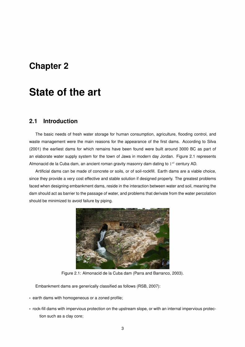
an elaborate water supply system for the town of Jawa in modern day Jordan. Figure 2.1 represents
Almonacid de la Cuba dam, an ancient roman gravity masonry dam dating to 1st century AD.
Artificial dams can be made of concrete or soils, or of soil-rockfill. Earth dams are a viable choice,
since they provide a very cost effective and stable solution if designed properly. The greatest problems
faced when designing embankment dams, reside in the interaction between water and soil, meaning the
dam should act as barrier to the passage of water, and problems that derivate from the water percolation
should be minimized to avoid failure by piping.
Figure 2.1: Almonacid de la Cuba dam (Parra and Barranco, 2003).
Embankment dams are generically classified as follows (RSB, 2007):
- earth dams with homogeneous or a zoned profile;
- rock-fill dams with impervious protection on the upstream slope, or with an internal impervious protec-
tion such as a clay core;
3

- mixed dams with the longitudinal profile divided in two embankments, one earth and another rock-fill
embankment or soil-rockfill mixtures;
There are also different types of embankment dams not covered by this classification because the
design of the dam is inherently conditioned by the materials available on site.
The previous classification is based on the distinction of the different types of materials used to build
earth and rock-fill embankments. The distinctive characteristics of the materials used are as follows:
- Materials used in the earth embankments, are mainly different types of soil that must guarantee both
impervious and strength characteristics. Other types of materials such as concrete, soil-cement
mix, steel, asphalt cement are used to create impervious walls inside the earth dam if the geoma-
terials available are not able to ensure the impervious characteristics.
- The different types of materials have an extensive grain size distribution.If soils, in general their pre-
dominant particle diameters smaller than 2 mm. The behavior of the embankment regarding the
compaction, deformation structural resistance and permeability is conditioned by the fine matrix
provided by the fine elements in the soil;
- Rock-fill material is defined by a high significant diameter (D50 < 2 m) and %(D = 50 mm) > 60% and
low presence of fine particles (< 5%), with Ksat > 10−51 (NEVES, 2002).
2.1.1 Types of embankment dams
Homogeneous Embankment Dams
Homogeneous embankment dams are generally composed by clay, sandy clay, clayey sand and clay
mixes.
Because the embankment is generally composed of one type of material, it should be able to give
the characteristics needed for a proper dam. The material must have low permeability, resistance and
high stiffness(or enough stiffness).
The whole embankment acts as a control system for water seepage. Seepage control devices such
as filter and drains are mandatory, and must be designed to avoid problems mainly associated to internal
erosion and piping phenomena.
Figure 2.2: General profile for homogeneous embankment dam. (Source: Narita, 2000).
The main aspect to account for in designing homogeneous embankment dams is the seepage con-
trol. The saturation curve must be kept far from the surface of the downstream face of the dam in order to1Hydraulic conductivity of saturated soil
4

avoid seepage in this slope and therefore failure by sliding in the downstream face. This can be ensured
by introducing a filter and a drain. The addition of a drain on the downstream toe of the dam is used to
avoid the problem, capable of capturing and draining the flow due to seepage trough the embankment’s
body and also trough the foundation. In figure 2.2 an example of the implementation of seepage control
devices such as filters is presented.
Zoned embankment dams
Zoned embankment dams are a natural follow up from homogeneous embankment dams, and are
very common because usually there is lack of fine materials near the dam site and the transportation
costs of the soil increase, rendering the project costly. Also different zones in the dam allows for steeper
inclines, making the dam use less material and therefore reducing cost. By zoning the dam profile,
materials can be selected according to the design criteria for that zone, for example, clay can be used in
the nucleus to make it impervious and a rock-fill layer can be used in the downstream slope and also in
the upstream slope to guarantee the mechanical resistance of the dam.
The general profile for a zoned embankment dam is composed by soil, rock-fill and a clay core. In
figure 2.3 an example of the profile for a layered embankment dam is provided.
Figure 2.3: General profile for a zoned embankement dam. (Source: Narita, 2000).
In addition to the soil zones, there also the seepage control devices such as filters and drain to
prevent internal erosion from the core.
Other types of zones dams have a synthetic impervious protection on the upstream slope or in the
center. Materials used can be concrete such as in rock-fill dams with a concrete wall, or asphalt cement
or even steel plates.
Rock-fill dams
Rock-fill embankment dams are a type of dam that have steeper slopes because of the naturally high
friction angle of the material. Water seepage is naturally a disadvantage of this types of embankments
due to the high permeability of rockfill material so seepage control mechanisms should be considered,
such as the introduction of a structural concrete wall on the upstream slope, which is generally con-
structed over a layer of carefully selected rock-fill, to allow for uniform support conditions of the concrete
5

layer, as well as avoiding sliding. The concrete layer is placed against this selected rockfill layer, with
sealed contraction joints, in order to prevent the concrete layer from cracking due to deformations pro-
duced by concrete retraction, embankment settlement, temperature variations and hydrostatic pressure.
Figure 2.4: Pego do altar Rock-fill dam with a steel layer on the upstream slope. (Source: O Leme -Imagens de Alcacer do Sal).
Other solutions include the ones presented with the layered embankment dams, such as an asphalt
cement layer, or a steel protection as presented in figure 2.4 in the Pego do Altar dam, where a steel
plate was used to cover the upstream slope.
2.1.2 Embankment dams. Geotechnical properties
Earthen embankments are mainly composed of clayey soil. Properties of the soil to account for in
embankments design are:
· type of soil;
· grain size distribution;
· consistency limits;
· soil classification;
· compaction curve (dry density and water content);
· internal friction angle;
Grain size
For embankment dams, the grain size distribution of the soil allows for quality control of the dam. The
construction process produces the refined grading size distributions in case of rockfill materials. In case
of fine materials, the respective grading size distribution must be controlled during placement, as well
as compaction characteristics. Each layer of the embankment must have homogeneous mechanical
properties throughout. The quality control using the grain size distribution of the soil is also used to
monitor the compaction process of the dam during, and after construction.
The size of the soil particles can be characterized by sieving tests, where the different grain size
fractions of soil are separated according to a certain specification, for example the E-219 specification,
6

and are used to obtain grain size distribution curves where one can identify the representative particle
diameter of a given amount of material that is captured by the screens.
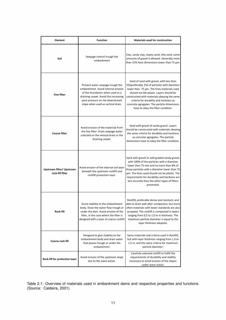
Table 2.1 shows materials used in different zones of the embankment, the respective uses and
properties.
Compaction
Compaction is a process to increase the resistance of the soil under constant water content condi-
tions. The stress applied to the soil leads the pore air to be displaced and the particles to rearrange.
Therefore this process increases resistance and decreases the permeability of the soil.
The process of compaction is different depending on the grains size of the soil. In fine soils, due to
the size of the grain, electromagnetic forces are predominant (attraction and repulsion), and are highly
dependent on water content. In granular soils, gravity is the predominant force that binds the particles
together trough friction. There is insensitivity to the moisture content on the soil, making it necessary to
rearrange the particles by vibrating the soil to acquire a denser soil by forcing the air out.
Water content of fine soils is vital to proper compaction. Water acts a lubricant within the soil, sliding
the particles together (INC., 2011). For each type of soil, for a given energy it is possible to define a
compaction curve as represented in figure 2.5.
There are two types of energy, given by the normal proctor method (D 698) and the modified proctor
method (D 1557). In the compaction curve a wet side and a dry side can be identified as being to the
left side of the optimum (lower water content) and to the right of the optimum (higher water content) for
which the soil behaves differently as it was stated above.
Figure 2.5: Compaction curve for different soils and compaction efforts. Comparison of different soilstructures induced by compaction effort. (Source: Cardoso, 2010).
This is an important characteristic of the soil to be used in earthen embankments, since the dam
7

is susceptible to some degree of imposed deformations and movements over time, and if the soil is to
rigid, cracks may appear and increase the rate of water flow trough the dam.This effect is particularly
degrading in zoned dams, since the core is commonly composed of clay soil, that has a high volumetric
expansion when in contact with water after drying.
Figure 2.7 represents silty clay compacted on the wet side leaving a smoother structure on the soil,
and much smaller pores and figure 2.6 represents a sample of the same soil but compacted on the dry
side, giving the soil a more flocculated structure (Alonso, 2004)
Figure 2.6: Silty clay compacted on the dryside. (Source: Alonso, 2004).
Figure 2.7: Silty clay compacted on the wetside. (Source: Alonso, 2004).
Embankment dams are usually compacted in the wet side of the reference curve in order to obtain
less rigid soil with less volumetric expansion during the wetting process and the cycles of wetting and
drying caused by the reservoir level variations during exploitation.
2.1.3 Elements of embankment design
Project Criteria
The fundamental project requirements for and embankment dam, regardless of the profile adopted
are:
- Hydraulic resistance. Safety criteria and protective measures against seepage and internal erosion.
Special attention must be given to scenarios of rapid filling and rapid draining of the dam as well
as the behavior during the first filling.
- Structural resistance, the embankment body should be able to support the water pressure and the
slopes must be stable in every design scenario during construction and exploration of the dam.
The safety requirements for embankment dams design are not limited to the sliding accidents of the
embankment slopes, and the most important aspects to consider have to do with water seepage. The
design criteria is verified whenever:
tanαd < tanφ′d (2.1)
where φ′d is the design effective internal friction angle of the material, αd is the design embankment
slope.
8
Upstream slope
The design for the upstream slope of the embankment dam is done for test scenarios during dam
construction and during rapid drawdown conditions (Marcelino, 2008). The failure of the upstream slope
is highly improbable for retention water level conditions since the oercolantion force acts as a stabilizing
force on the upstream side of the embankment.
During construction if the soil used in the upstream embankment body has a high amount of fine
material and the water content is close to or above the optimum, pore pressure is generated by the com-
paction efforts and by increasing gravity forces. This is the only situation when safety must be checked
during construction. In service, for rapid drawdown conditions, if the material in the shoulders has low
permeability (figure 2.8), pore pressure located in the upstream body do not have time to dissipate, in
this case there is the inversion of the water flow trough the dam, causing the percolation force to be
instabilizing.
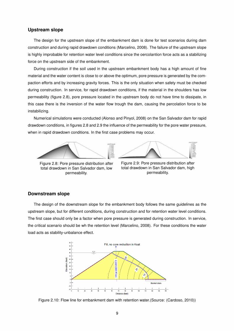
Numerical simulations were conducted (Alonso and Pinyol, 2008) on the San Salvador dam for rapid
drawdown conditions, in figures 2.8 and 2.9 the influence of the permeability for the pore water pressure,
when in rapid drawdown conditions. In the first case problems may occur.
Figure 2.8: Pore pressure distribution aftertotal drawdown in San Salvador dam, low
permeability.
Figure 2.9: Pore pressure distribution aftertotal drawdown in San Salvador dam, high
permeability.
Downstream slope
The design of the downstream slope for the embankment body follows the same guidelines as the
upstream slope, but for different conditions, during construction and for retention water level conditions.
The first case should only be a factor when pore pressure is generated during construction. In service,
the critical scenario should be wh the retention level (Marcelino, 2008). For these conditions the water
load acts as stability-unbalance effect.
Figure 2.10: Flow line for embankment dam with retention water.(Source: (Cardoso, 2010))
9

The result is a higher αd leading to a steeper slope compared to upstream, due to the fact that failure
conditions are not influenced by rapid drawdown scenarios.
On the contrary, internal erosion phenomena needs a much more detailed design and analysis with
a higher risk of failure. For example construction defects associated with the filters could lead to internal
erosion of the core or to piping failure, or to the transport of material from the core to the voids on the
rock-fill or embankment layers downstream. Internal erosion corresponds to the phenomena of transport
of soil particles from the inside of the dam, by water seepage forces. Internal erosion tends to propagate
upstream from an outlet point downstream, trough water passages in the dam, or pipes, until it reaches
the upstream slope of the dam or the foundation surface also upstream. This type of failure is called
piping and is one of the fastest to lead to the dam breaching.
Geological and geotechnical studies should be performed in order to gather information on the type
and characteristics of the soil, localization of the ground-water level, local conditions, identification of
geotechnical singularities such as seismic faults and others.
10
SoilSeepage control trough the
embankment
Clay, sandy clay, clayey sand, silty sand, some
amounts of gravel is allowed. Generally more
than 15% have dimensions lower than 75 µm.
Fine filter
Prevent water seepage trough the
embankment. Avoid internal erosion
of the foundation when used as a
draining carpet. Avoid the increasing
pore pressure on rhe downstream
slope when used as vertical drain.
Sand of sand with gravel, with less than
5%(preferably 2%) of particles with diamiters
lower than 75 µm. The fines materials used
should not ble plastic. Layers should be
constructed with materials obeying the same
criteria for durablity and hardness as
concrete agregates. The particle dimensions
have to obey the filter condition.
Coarse filter
Avoid erosion of the materials from
the fine filter. Drain seepage water
colected on the vertical drain or the
draining carpet.
Sand with gravel of sandy gravel. Layers
should be constructed with materials obeying
the same criteria for durablity and hardness
as concrete agregates. The particle
dimensions have to obey the filter condition.
Upstream filter/ Upstream
rock-fill filter
Avoid erosion of the internal soil layer
beneath the upstream rockfill and
rockfill protection layer.
Sand with gravel or well graded sandy gravel,
with 100% of the particles with a diameter
lower than 75 mm and no more than 8% of
those particles with a diameter lower than 75
µm. The fines used should not be plastic. The
requirements for durability and hardness are
less accurate than the other types of filters
presented.
Rock-fill
Grant stability to the embankment
body. Drain the water flow trough or
under the dam. Avoid erosion of the
filter, in the case where the filter is
designed with a layer of coarse rockfill
Rockfill, preferably dense and resistant, and
able to drain well after compaction, but more
often materials with lower standards are also
accepted. The rockfill is compacted in layers
ranging from 0,5 to 1,0 m in thickness. The
maximum particle diameter is equal to the
layer thickness adopted.
Coarse rock-fill
Designed to give stability to the
embankment body and drain water
that passes trough or under the
embankment.
Same materials and criteria used in Rockfill,
but with layer thickness ranging from 1,0 to
1,5 m, and the same criteria for maximum
particle diameter.
Rock-fill for protection layerAvoid erosion of the upstream slope
due to the wave action.
Carefully selected rockfill to fulfill the
requirements of durability and stablity
necessary to avoid erosion of the slopes
under wave action.
Element Function Materials used for construction
Table 2.1: Overview of materials used in embankment dams and respective properties and functions.(Source: Caldeira, 2001).
11

12

2.2 Failure of Embankment Dams
2.2.1 Failure concept applied to embankment dams
Dam safety comprises the following criteria (RSB, 2007):
- Structural safety corresponding to the endurance and ability to satisfy the structural behavior demands
related to performance in exploration situations as well as exceptional conditions and loads.
- Hydraulic safety regarding the behavior of the security devices and exploration components of the
dam, as well as the filtering, waterproofing and draining systems.
- Operational safety corresponding to the capability of the dam to satisfy the behavior criteria related to
operation and functionality of the equipments and safety and exploration components.
- Environmental safety corresponding to the ability of the dam to keep the demands for behavior rel-
ative limitation of incidents that might cause harm to the environment, namely to populated and
productive areas.
Should any of these criteria not be met, the dam can be considered as in failure.
According to Singh (1996) the most common causes and modes of failure of earth dams are:
1 - overtopping caused by extreme floods;
2 - structural failure due to internal erosion (piping);
3 - structural failure due to shear slide;
4 - structural failure due to foundation defects;
5 - failure due to natural or induced seismicity;
This work will focus on structural failures related to intense precipitation events,earthquakes or any
other actions that may cause a breach in the dam, leading to the flooding of the downstream areas.
2.2.2 Failure by Overtopping
The following section will focus on the first cause of earth dam failure, overtopping, giving the base
mechanics of the process of failure and their main causes. A brief revision is made on the recent ad-
vances in dam breaching, most notably the implementation of algorithm to simulate the sudden collapse
of parts of the breach wall, also known as sliding.
Three elements are included in the hydraulics of flow over the dam: flow over the crest, flow trough
the breach and flow trough the breach channel on the downstream face of the dam. When the flow
passes over the crest, the breach is formed.
The erosive force is highest on the downstream slope of the dam, because of the higher velocities
the flow attains. The extent of erosion and subsequent sediment transport depend upon the extent of
overtopping, material composition, downstream conditions (Singh, 1996).
13
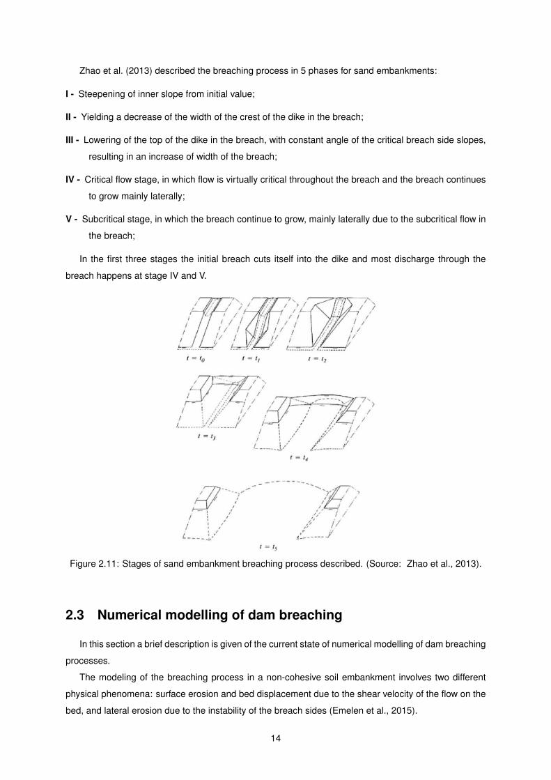
Zhao et al. (2013) described the breaching process in 5 phases for sand embankments:
I - Steepening of inner slope from initial value;
II - Yielding a decrease of the width of the crest of the dike in the breach;
III - Lowering of the top of the dike in the breach, with constant angle of the critical breach side slopes,
resulting in an increase of width of the breach;
IV - Critical flow stage, in which flow is virtually critical throughout the breach and the breach continues
to grow mainly laterally;
V - Subcritical stage, in which the breach continue to grow, mainly laterally due to the subcritical flow in
the breach;
In the first three stages the initial breach cuts itself into the dike and most discharge through the
breach happens at stage IV and V.
Figure 2.11: Stages of sand embankment breaching process described. (Source: Zhao et al., 2013).
2.3 Numerical modelling of dam breaching
In this section a brief description is given of the current state of numerical modelling of dam breaching
processes.
The modeling of the breaching process in a non-cohesive soil embankment involves two different
physical phenomena: surface erosion and bed displacement due to the shear velocity of the flow on the
bed, and lateral erosion due to the instability of the breach sides (Emelen et al., 2015).
14

The first is a phenomena resulting from the interaction between the fluid layer (clear water layer
and contact or transport layer) and the sediment bed. If the stresses on the boundary of the contact
layer are not in equilibrium with the bed, there will be a bed variation as a consequence in the form of
erosion. There is an equilibrium length or adaptation length, which is the distance needed for erosion
and deposition phenomena to be in equilibrium i.e. for the bed variation over time to become null.
Surface erosion can be modelled by introducing a sediment conservation equation, coupled with the
shallow water equations that relate the conservation of mass and momentum within a domain.
The second is is gravitational induce side wall failures (Volz et al., 2010).The failures occur spon-
taneously over the breaching duration and are usually the main cause for the lateral widening of the
breach channel. Failure types can differ largely depending on various factors as e.g. the soil material,
the seepage line and the pore pressures within the soil matrix. The majority of the observed failures
types are a mix of fall and slide failure (Pickert et al., 2004).
Emelen et al. (2015) tested several sediment transport formulations, and some bearing angles for
slope instabilization which where validated with laboratory experiments conducted in the Hydraulics
Laboratory of the Universite Catholique de Louvain, Belgium (Spinewine et al., 2004).
The numerical formulation used for the dam breaching simulations was:
δU
δt+δF (U)
δx+δG(U)
δy= S; (2.2)
U =
h
uh
vh
zb
; F =
uh
u2h+ gh2
2
uvh
qs,x1−ε0
; G =
uh
uvh
v2h+ gh2
2
qs,y1−ε0
; S =
0
gh(Sox− Sfx)
gh(Soy − Sfy)
0
; (2.3)
where x and y represent the components in x and y directions, respectively, and u and v are the
depth averaged velocities in the x- and y-directions. qs represented the sediment rate discharge and
was estimated using a large number of well known empirical formulas.
The 2D bank-failure operator was developed and inserted into the classical 2D shallow model by
Swartenbroekx et al. (2010). The operator is based on a local bank-failure criterion: the slope of each
cell is calculated in order to analyse its stability. When the slope of a cell exceeds a critical angle αc, the
bank-failure is activated and cells are tilted until reaching a residual angle αr
The numerical simulations obtained, presented in figure 2.12 show a good representation of the
breaching process of sand dams. Tough is rarely the case, as explained in the previous chapter, design
criteria for embankment construction are very demanding in terms of the materials used and construction
techniques, thus, rendering the real life behavior of a dam when in a situation of overtopping very
different, more notably the existence of undercutting when water is eroding the sides of the breach,
which in turn leads to mass displacement phenomena and instantaneous breach enlargement. This
phenomena does not occur in sand dikes.
15

Figure 2.12: Dam breaching numerical simulation. (Source: Emelen et al., 2015).
Dual mesh approach
Using the same criteria for sliding failure, i.e. the critical slope angle, Volz et al. (2010) used a
2D dual mesh physically based model to simulate embankment dam breaching using surface erosion
and geotechnical failure mechanisms. It used a separate mesh for the bottom, differentiating different
significant grain diameter classes in order to better simulate the fluid-water interactions in the contact
load layer. The discretization scheme is represented in figure 2.13.
Figure 2.13: Discretization scheme for the dual mesh approach. (Source: Volz et al., 2010).
16

An Euler-scheme and Riemann-solver were applied to calculate the fluxes at the edges of the cells
and for the solution of the balance equations an uncoupled, quasi-steady solution procedure was cho-
sen.
The dual mesh approach leads to several numerical problems that can be summarized as (Volz et al.,
2010) and represented in figure 2.14.
- Changes in the sediment volume of a cell by in- or out-flowing sediment fluxes must be distributed in
an appropriate way on the nodes of this cell. However, the distribution of the sediment volume is
not unique and it is not clear by which criteria it should be done
- Changes in bed elevation of a cell’s node do not only affect the sediment volume of this cell, but also
the sediment volumes of all adjacent cells. This is problematic regarding the conservation of the
sediment masses
- These mutual influences between adjacent cells correspond to diffusive fluxes between the cells. In
case of fractional transport this may lead to an undesired mixing of the grain compositions.
Figure 2.14: Dual mesh approach, numerical problems. (Source: Volz et al., 2010).
Numerical simulations of dam breaching where carried out, using and MPM (Meyer-Petter & Muller)
formula to model surface erosion and a critical slope angle for sliding failure. The dam was divided in
half, assuming symmetry in the response of the dam to the flow, to aid in computational efficiency.
Figure 2.15: Simulated dam breach. (Source: Volz et al., 2010).
The results shown in figure 2.15 where compared with experimental data obtained by Pickert et al.
(2011), where embankment dams where made similar fashion to the numerical model, i.e. only half of the
dam was represented and symmetry along the longitudinal dimension of the dam was assumed, allowing
17

for a glass wall to be installed and monitor the breaching. The embankment was built up with three
different uniform granular sands on a fixed bed.The comparison between numerical and experimental
results is presented in figure 2.16.
Figure 2.16: Dam breaching results and comparison with experimental data. (Source: Volz et al., 2010).
The results seem to show good agreement with the sand embankment breaching, and it is noted that
one of the shortcomings of the lateral erosion modeling is that it occurs steadily and and continuously,
which leads to small changes in the side wall slopes during the breaching, instead of massive events
that lead to instantaneous breach enlargement (Volz et al., 2010).
The cases presented in this chapter study the breaching of sand embankments and are able to
reproduce the breaching to some degree of accuracy, but earth dams are mainly composed of cohesive
soil, and thus the breaching process is different due to the nature of the material, but also difficult to
test due to the specifications needed to build properly compacted embankments and to the difficulty
associated to characterize the complex breaching process of embankment dams.
18
Chapter 3
Dam breach experiments for model
validation
3.1 Introduction
Experimental work was considered as a way of validating the numerical model. A reliable character-
ization of the breaching of embankment dams is crucial for a good calibration of the numerical model.
The experimental work was conducted at the National Laboratory of Civil Engineering (LNEC), in
Lisbon, Portugal. Four experiments where undertaken in total. Between experiments, initial breach
geometry and moisture content of the soil where changed to analyze the influence of each in the dam
breaching process.
For this work it is reminded that the main objective of the experiments is to provide outflow hydro-
graphs and a good documentation of the breaching experiments, that can be used to calibrate and/or
validate the numerical model.
3.2 Overview of experimental setup
Figure 3.1 shows the floor plan and profile of the experimental setup, the following section will present
the different equipments used in the experimental setups.
The model is not aimed at reproducing a real embankment dam. The goal is to induce dam breach-
ing, while maintaining the cohesive nature of the dam material and compaction properties, which are
observed in real life scenarios, but within a time frame suitable for the experiments, as due to the con-
straints of the experimental setup i.e. reservoir capacity and available materials and work conditions. In
laboratory environment, if the criteria used for the models construction, would be the same as those for
real dams, breaching would take too long to occur to be feasible.
19

Q
2.61
21
Q
6.60
7.00
0.2615.59
2.961.60
4.700.20
0.9031.50
1.60
2.00
1.65
0.851.25
0.23
0.70
1.00
0.20
1.20
2.30
1
34
5
1112
2
1.00
LE
GE
ND
1 - F
low
inlet(Ø
350 m
m)
2 - Brick w
all to still the flow at the reservoir inlet
3 - Resitive P
robe (R1)
4 - Resitive P
robe (R2)
5 - Resitive P
robe (R4)
6 - Resitive P
robe (R3)
7 - Resitive P
robe (R5)
8 - Dispensador de poliestireno
9 - Acoustic probes
10 - Em
bankment
11 - Stilling pool
11 - Dow
nstream spillw
ay
01
2m
Reservoir
Vmax≈45m
³
10
10
9
1010101010
1010101010
1010101010
1010101010
1.50
0.11
2.10
1.50
0.50
0.10
2.501.00
0.43
6
2.90
0.45
7
8 8
810
Figure3.1:
Experim
entalFacilityfordam
breachexperim
ents
20

The set-up consists of a channel 31.5 m long, between 6.60− 1.70 m wide and between 0.5− 1.30 m
deep. At the downstream end of the channel there are a sediment supply tank with 1.7 m width, 4.4 m
length and a maximum depth of 0.60 m, and a rectangular spillway.
The inlet, outlet and reservoir are instrumented with a flow meter and a total of six resistive probes
respectively. A control volume sufficiently near the breach channel is instrumented with seven acoustic
probes on the boundaries, two high speed motion capture cameras, one pointing downwards to the
control volume, and the other pointing to the upstream face of the dam, in the direction of the breach
channel. A laser equipped with prismatic lens is also implemented directly over the breach channel. A
physical trigger in the form of a button was used to synchronize the data acquisition from the probes.
Upstream Inlet
The water storage in the underground reservoir is pumped to a reservoir located at higher altitude,
and conducted to the channel by gravity. Due to the importance of maintaining a stable water surface
level in the reservoir, a flow meter monitors the inflow. The structure seen in figure 3.1 2 is a brick wall
designed to dissipate energy so that the laminar flow can be considered.
Spillway
The spillway (3.1, 11) will discharge the water volume from the embankment. It is equipped with
a resistive probe to monitor the water height, and with an appropriate spillway equation, a an outlet
discharge can be estimated.
21
3.3 Equipment and software
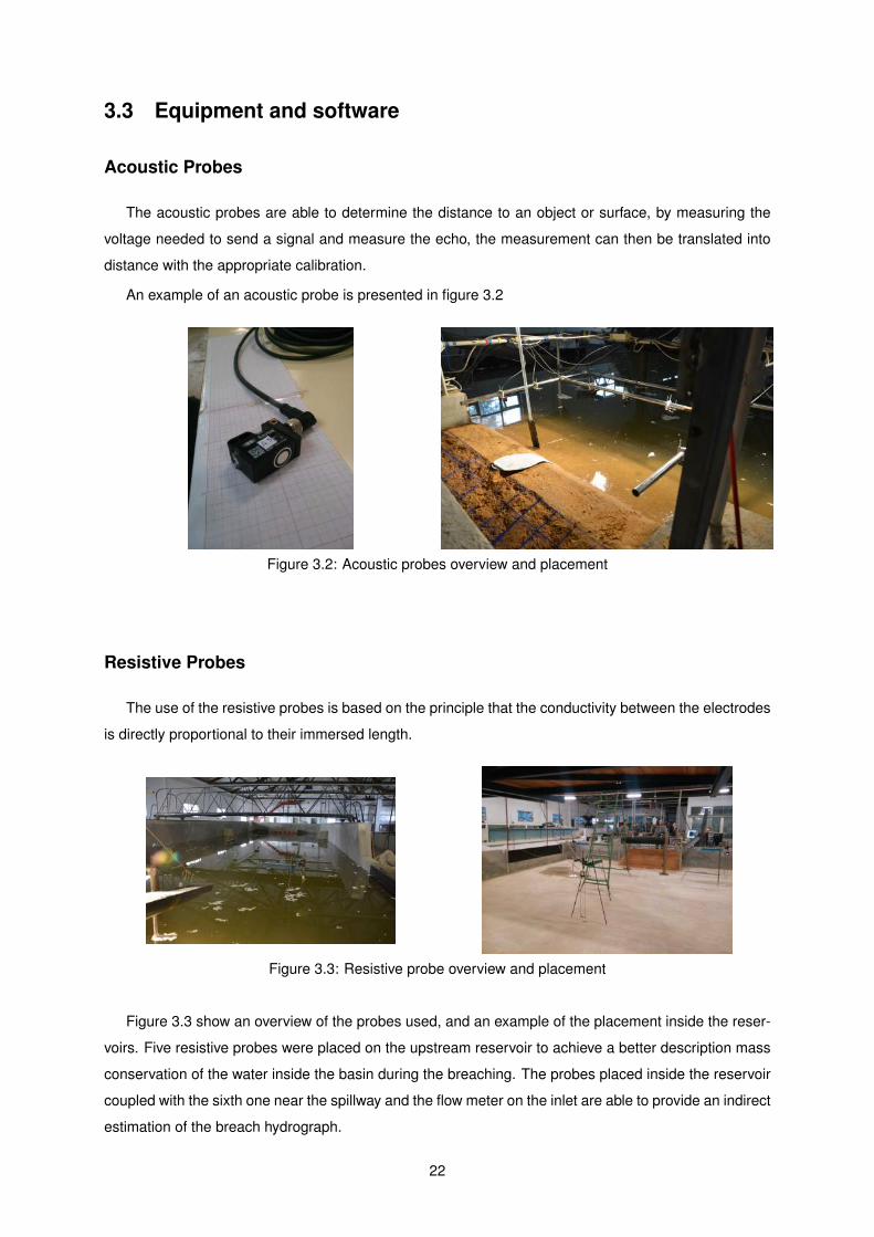
Acoustic Probes
The acoustic probes are able to determine the distance to an object or surface, by measuring the
voltage needed to send a signal and measure the echo, the measurement can then be translated into
distance with the appropriate calibration.
An example of an acoustic probe is presented in figure 3.2
Figure 3.2: Acoustic probes overview and placement
Resistive Probes
The use of the resistive probes is based on the principle that the conductivity between the electrodes
is directly proportional to their immersed length.
Figure 3.3: Resistive probe overview and placement
Figure 3.3 show an overview of the probes used, and an example of the placement inside the reser-
voirs. Five resistive probes were placed on the upstream reservoir to achieve a better description mass
conservation of the water inside the basin during the breaching. The probes placed inside the reservoir
coupled with the sixth one near the spillway and the flow meter on the inlet are able to provide an indirect
estimation of the breach hydrograph.
22

Spider8
The hardware Spider8 was used to control and synchronize the data from the resistive probes and
is presented in figure 3.4.
Figure 3.4: Spider8 signal amplifier
CatmanEasy
The data capturing software CatmanEasy was used to perform the data acquisition of the resistive
probes and the flowmeter.
National Instruments data acquisition board
A data acquisition board made by National Instruments was used to acquire the data from the resis-
tive probes and is presented in figure 3.5.
Figure 3.5: National instruments data acquisition board
LabView Signalexpress
The data acquisition software LabView Signalexpress was used to capture the data from the seven
acoustic probes.
23

Trigger for data acquisition
Due to the nature of the equipments used and their compatibility with the various capture boards and
different softwares, there is a need to carefully synchronize the data acquisition from all the probes in-
volved, hence a physical trigger was developed to send a user generated tension peak that is registered
at the same time in both data acquisition softwares and boards.
The external trigger is presented in figure 3.6.
Figure 3.6: Analogic Trigger for data synchronization
Photonfocus high speed camera
The Photonfocus high speed camera presented in figure 3.7 was used to document the dam breach-
ing evolution. The camera was placed facing the upstream slope of the dam. Refraction effects of the
camera lens where taken into account, as well as distance to the embankment breach and angle of the
camera.
Figure 3.7: Photonfocus camera
Mikrotron high speed camera
The Mikrotron high speed camera was used to record images of the dam breaching process but
more importantly, to monitor the passing of carefully selected styrofoam balls inside the control volume,
so that a PIV algorithm can be applied and the velocity field near the breach channel can be estimated.
This requires the acquisition framerate of the camera to be high and consistent enough that the position
of the styrofoam balls can be tracked between two consecutive frames. The camera is presented in
figure 3.8.
24

Figure 3.8: Mikrotron high speed camera setup
Ilumination setup
The high speed cameras need to be able to distinguish and isolate the styrofoam balls, and as such
the experimental setup requires homogeneous lighting conditions inside the control volume, this was
achieved by using a very low environment light, coupled with spotlights pointing to the control volume,
as represented in figure 3.9.
Figure 3.9: Ilumination setup and purpose
Laser Quantum Finesse
The Laser was used to accentuate the dam breach geometry, when captured by the Photon Focus
camera. A prismatic lens was placed directly under the laser and rotated so that the laser turns into a
sheet of light, which when pointed towards the dam breach, should provide an accurate reading of the
breach geometry. The laser is presented in figure 3.10.
3.4 Dam breaching experiments
3.4.1 Characterization of the embankments
Tests where performed to evaluate the geotechnical characteristics of the soil in order to choose a
compaction method and effort adequate for the models. If the dam is built with realistic design param-
25
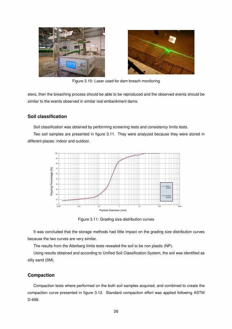
Figure 3.10: Laser used for dam breach monitoring
eters, then the breaching process should be able to be reproduced and the observed events should be
similar to the events observed in similar real embankment dams.
Soil classification
Soil classification was obtained by performing screening tests and consistency limits tests.
Two soil samples are presented in figure 3.11. They were analyzed because they were stored in
different places: indoor and outdoor.
Diagrama
Page 1
0
10
20
30
40
50
60
70
80
90
100
0,001 0,01 0,1 1 10 100 1000
Pas
sing
Per
cent
age
(%)
Particle Diameter (mm)
IndoorSample
OutdoorSample
Figure 3.11: Grading size distribution curves
It was concluded that the storage methods had little impact on the grading size distribution curves
because the two curves are very similar.
The results from the Atterberg limits tests revealed the soil to be non plastic (NP).
Using results obtained and according to Unified Soil Classification System, the soil was identified as
silty sand (SM).
Compaction
Compaction tests where performed on the both soil samples acquired, and combined to create the
compaction curve presented in figure 3.12. Standard compaction effort was applied following ASTM
D-698.
26

17,8
18
18,2
18,4
18,6
18,8
19
19,2
19,4
19,6
4 5 6 7 8 9 10 11 12 13
γ d(kN/m
3 )
w(%)
Figure 3.12: Combined compaction curve for both samples
The optimum point was identified and is presented in table 3.1.
Table 3.1: Optimum point for compaction curve
This curve provides the optimum dry density and water content for compaction of a real embankment,
however, model scale has to be accounted for, or else breaching will not occur. For this reason, a new
compaction curve was obtained using 25% of the energy in the standard proctor test. The curve obtained
is presented in figure 3.11.
17,00
17,50
18,00
18,50
19,00
19,50
20,00
20,50
5 6 7 8 9 10 11 12 13 14 15
γ d(k
N/m
3)
w(%)
Figure 3.13: Compaction curve for 25% energy
The equipment used for compaction of the experimental embankments was the manual compactor
PC1010 of Euroshatal weighting 46 kg, with a compaction area of 430 m2/h and a vibration frequency of
100 Hz and is presented in figure 3.14.
More information about the experimental setup and embankment construction can be found in B.2
and in Santos (2015).
27
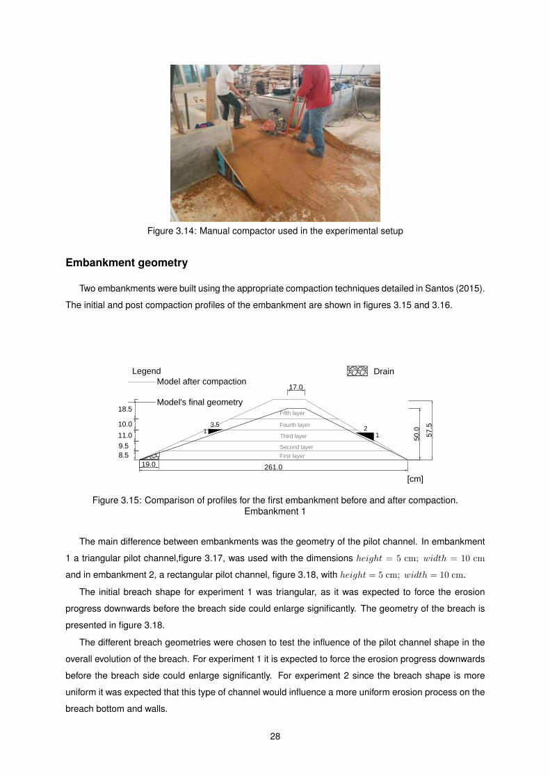
Figure 3.14: Manual compactor used in the experimental setup
Embankment geometry
Two embankments were built using the appropriate compaction techniques detailed in Santos (2015).
The initial and post compaction profiles of the embankment are shown in figures 3.15 and 3.16.
3.51 2
1 50.0
57.5
19.0
18.5
8.59.5
11.0
10.0
261.0
17.0
[cm]
LegendModel after compaction
Model's final geometry
Drain
First layer
Second layer
Third layer
Fourth layer
Fifth layer
Figure 3.15: Comparison of profiles for the first embankment before and after compaction.Embankment 1
The main difference between embankments was the geometry of the pilot channel. In embankment
1 a triangular pilot channel,figure 3.17, was used with the dimensions height = 5 cm; width = 10 cm
and in embankment 2, a rectangular pilot channel, figure 3.18, with height = 5 cm; width = 10 cm.
The initial breach shape for experiment 1 was triangular, as it was expected to force the erosion
progress downwards before the breach side could enlarge significantly. The geometry of the breach is
presented in figure 3.18.
The different breach geometries were chosen to test the influence of the pilot channel shape in the
overall evolution of the breach. For experiment 1 it is expected to force the erosion progress downwards
before the breach side could enlarge significantly. For experiment 2 since the breach shape is more
uniform it was expected that this type of channel would influence a more uniform erosion process on the
breach bottom and walls.
28

3.51 2
1
LegendModel after compaction
Model's final geometry
6
50.0
56.5
16.0
13.0
10.312.0
11.0
10.2
261.0
Drain
[cm]
First layer
Second layer
Third layer
Fourth layer
Fifth layer
Figure 3.16: Comparison of profiles for the second embankment before and after compaction.Embankment 2
Figure 3.17: Initial breach geometry forexperiment 1
Figure 3.18: Initial breach geometry forexperiment 2
It is worth to mention that a drain was also built bellow the downstream slope in order to simulate an
homogeneous dam. This drain might have influence in the overall evolution of the breach as discussed
by Santos (2015). The drain is presented in figure 3.19
Figure 3.19: Drain placed at the toe of the embankment model.
29

Data collected and outflow hydrograph
As explained in the beginning of the chapter the probes placed on the experimental setup where
used to gather water surface elevation, inside the reservoir, inside the area of influence near the breach
and in the downstream spillway. Image and video recordings where taken from the high speed cameras
and HD recording cameras placed in the setup.
The surface elevation measurements taken for the probes are presented in Figures 3.20 and 3.21
along with the discharge measured from the Resistive probe R6 placed on the spillway.
0 1000 2000 3000 4000 5000 6000 7000 8000 90000
0.2
0.4
Time (s)
Qin
! m3s!
1"
0 1000 2000 3000 4000 5000 6000 7000 8000 9000-0.2
0
0.2
Z(m
)Figure 3.20: Surface elevation measurements for all probes vs discharged measured. Trial 1
0 500 1000 1500 2000 2500 3000 35000
0.05
0.1
0.15
0.2
0.25
Time (s)
Qin
! m3s!
1"
0 500 1000 1500 2000 2500 3000 3500-0.6
-0.4
-0.2
0
0.2
0.4
Z(m
)
Figure 3.21: Surface elevation measurements for all probes vs discharged measured. Trial 2
The Discharge is measured at the inlet. In the outlet a spillway equation is applied using the elevation
measurements taken from the probe. The discharge is then calculated by:
Qspill = 140.74H3 − 5.38H2 + 0.4H (3.1)
30

In the reservoir the discharge upstream of the breach channel is calculated using the conservation
of mass equation inside the reservoir area. An influence area is attributed to each probe, by voronoi
polygons as presented in figure 3.22
-30 -25 -20 -15 -10 -5 0 5-15
-10
-5
0
5
10
15
coordinate x (m)
coor
din
ate
y(m
)
a) Trial 1
-30 -25 -20 -15 -10 -5 0 5-15
-10
-5
0
5
10
15
coordinate x (m)
coor
din
ate
y(m
)b) Trial 2
Figure 3.22: Influence areas for probes using Voronoi polygons
The flow upstream of the breach is then given by:
Qout = Qin −Area×δZ
δt(3.2)
where Qin is the discharge measured by the flow-meter, Qout is the discharge trough the breach,
calculated upstream.
The data from the probes is then filtered and averaged to obtain the outflow hydrographs, presented
in figures 3.23 and 3.24.
31

1800 2700 3600 4500 5400 6300 7200 81000
0.1
0.2
0.3
Time (s)
Disch
arg
e! m
3s"
In.ow Out.ow - simple average Out.ow - weighted average Out.ow - Resistive probe R6
Figure 3.23: Outflow hydrographs for trial 1
1600 2000 2400 2800 3200-0.1
0
0.1
0.2
0.3
0.4
0.5
Time (s)
Disch
arge! m
3s"
In.ow Out.ow - simple average Out.ow - weighted average Out.ow - Resistive probe R6
Figure 3.24: Outflow hydrographs for trial 2
32

Chapter 4
Numerical Model
4.1 Introduction
This chapter is aimed at the presentation of the numerical model used for the dam break simula-
tions. The model was developed based on the conceptual model proposed by Ferreira (2005) which
features conservation equations derived within the continuum approach for an idealized layered domain
composed by the bed, transport layer and clear water layer.
Figure 4.1: Layered flow structure composed by the bed or bottom, the transport or contact layer andthe clear water layer. (Source: Guan et al., 2014).
The shallow water approach is introduced in the depth-averaging of the Navier-Stokes equations,
by assuming that the horizontal length scale is much greater than the vertical length scale. Under this
condition, conservation of mass implies that the vertical velocity of the fluid is small enough that it can
be removed from the equation. It can be shown from the momentum equation that the vertical pressure
gradients are nearly hydrostatic, and that horizontal pressure gradients are due to the displacement of
the pressure surface, implying that the velocity field is constant throughout the fluid depth (Canelas et al.,
2013).
The system of conservation equations is closed by equations the describe flow resistance, for par-
ticular rheologies, and bed-flow interactions.
The numerical model is then used to compute a number of well defined initial value problem with
analytical solutions on a structured square mesh.
The software used to compute the numerical solutions is Matlab, which features flexible debugging
33
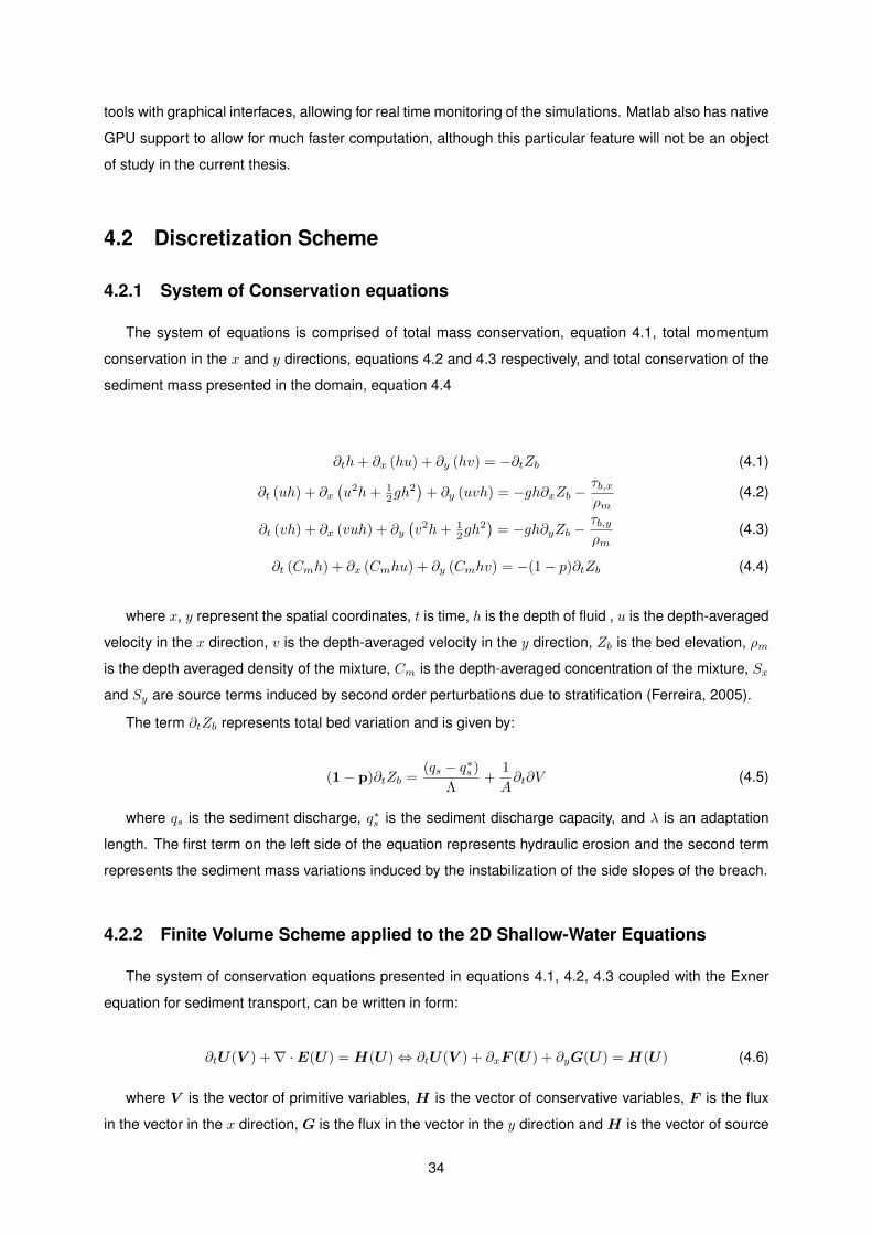
tools with graphical interfaces, allowing for real time monitoring of the simulations. Matlab also has native
GPU support to allow for much faster computation, although this particular feature will not be an object
of study in the current thesis.
4.2 Discretization Scheme
4.2.1 System of Conservation equations
The system of equations is comprised of total mass conservation, equation 4.1, total momentum
conservation in the x and y directions, equations 4.2 and 4.3 respectively, and total conservation of the
sediment mass presented in the domain, equation 4.4
∂th+ ∂x (hu) + ∂y (hv) = −∂tZb (4.1)
∂t (uh) + ∂x(u2h+ 1
2gh2)
+ ∂y (uvh) = −gh∂xZb −τb,xρm
(4.2)
∂t (vh) + ∂x (vuh) + ∂y(v2h+ 1
2gh2)
= −gh∂yZb −τb,yρm
(4.3)
∂t (Cmh) + ∂x (Cmhu) + ∂y (Cmhv) = −(1− p)∂tZb (4.4)
where x, y represent the spatial coordinates, t is time, h is the depth of fluid , u is the depth-averaged
velocity in the x direction, v is the depth-averaged velocity in the y direction, Zb is the bed elevation, ρm
is the depth averaged density of the mixture, Cm is the depth-averaged concentration of the mixture, Sx
and Sy are source terms induced by second order perturbations due to stratification (Ferreira, 2005).
The term ∂tZb represents total bed variation and is given by:
(1− p)∂tZb =(qs − q∗s )
Λ+
1
A∂t∂V (4.5)
where qs is the sediment discharge, q∗s is the sediment discharge capacity, and λ is an adaptation
length. The first term on the left side of the equation represents hydraulic erosion and the second term
represents the sediment mass variations induced by the instabilization of the side slopes of the breach.
4.2.2 Finite Volume Scheme applied to the 2D Shallow-Water Equations
The system of conservation equations presented in equations 4.1, 4.2, 4.3 coupled with the Exner
equation for sediment transport, can be written in form:
∂tU(V ) +∇ ·E(U) = H(U)⇔ ∂tU(V ) + ∂xF (U) + ∂yG(U) = H(U) (4.6)
where V is the vector of primitive variables, H is the vector of conservative variables, F is the flux
in the vector in the x direction, G is the flux in the vector in the y direction and H is the vector of source
34

terms, the later of which can be subdived as H = R+T +S, where R expresses the friction and vertical
fluxes, T represents the bottom source terms and S relates to the stratification and variation of density.
The dependent non-conservative variables in V , conservative variables in H and fluxes in F and G
are:
V =
h
u
v
Cm
; U =
h
uh
vh
Cmh
; F =
uh
u2h+ 12gh
2
uvh
Cmhu
; G =
vh
vuh
v2h+ 12gh
2
Cmhv
(4.7)
and the source terms in R and T are:
R =
−∂tZb− τb,xρ(w)
− τb,yρ(w)
−(1− p)∂tZb
; T =
0
−gh∂xZb−gh∂yZb
0
. (4.8)
The Finite Volume Method (FVM) discretization is then obtained by integrating the system of equa-
tions 4.6 in a cell i, and the Gauss theorem is then applied to the divergence term ∇ ·E(U) to obtain:
∂t
∫Ωi
U(V )dS +
∮Γi
E (U) · ndl =
∫Ωi
H(U)dS (4.9)
where E · n = Fnx + Gny with n = (nx, ny)T being the outward normal to cell Ωi.
Assuming the representation is piecewise, and that the cell area is Ai, and performing the boundary
integral on the ni edges of the cell i, one obtains from equation 4.9:
∂tAi 〈U i〉+
N∑k=1
Lk〈E · n〉ik = Ai 〈Hi〉 (4.10)
where 〈〉 represents the spatial average in the cell and Lk is the length of the k edge.
The flux variations can be expressed as a function of the conservative variables using a Jacobian
matrix, orthogonal to the edge in question. Since the flux vectors are not homogeneous functions
of the dependent variables, for the shallow water types system, it is usually not possible to obtain a
diagonal matrix for the Jacobian for x and y directions simultaneously, thus, an approximate Jacobian
matrix (Canelas, 2010; Toro, 2001) is used for the homogeneous part of the flux. The fluxes are then
susceptible to be represented in a eigenvector based homogeneous system,
∆ik 〈E · n〉 = (〈Ej〉 − 〈Ei〉) · nik =
N∑n=1
λ(n)ik α
(n)ik e
(n)ik (4.11)
whereN denotes the dimension of the eigenspace, in this caseN = 4 since there are three continuity
equations plus one sediment conservation equation. λ(n) is the n eigenvalue of the system, α(n)ik are
coefficients to represent wave strength and e(n)ik is the n eigenvector of the edge k pointing to the exterior
35

of the cell i.
The averaged variables are u, v,c (velocity of small perturbations) and Cm are:
uik =ui√hi + uj
√hj√
hi +√hj
; vik =vi√hi + vj
√hj√
hi +√hj
; cik =
√ghi + hj
2; Cmik
=Cmi
√hi + Cmj
√hj√
hi +√hj
(4.12)
With the average variables, the corresponding eigenvalues and eigenvectors are the calculated and
given by:
λ(1)ik = (u · n− c)ik; λ
(2)ik = (u · n)ik; λ
(3)ik = (u · n + c)ik; λ
(4)ik = (u · n)ik (4.13)
e(1)ik =
1
u− cnxv − cnyCm
ik
; e(2)ik =
0
−cnycnx
0
ik
; e(3)ik =
1
u+ cnx
v + cny
Cm
ik
; e(4)ik =
0
0
0
1
ik
(4.14)
where in eq. 4.13 u represents the velocity vector, c is the average small perturbation wave strength
and n is the exterior normal vector to the edge.
The wave-strengths α(n)ik associated to each variable are given by,
α(1)ik = ∆ik〈h〉
2 − 12cik
(∆ik 〈uh〉 − uik∆ik 〈h〉) · nik
α(2)ik = 1
cik(∆ik 〈uh〉 − uik∆ik 〈h〉) · tik
α(3)ik = ∆ik〈h〉
2 + 12cik
(∆ik 〈uh〉 − uik∆ik 〈h〉) · nik
α(4)ik = ∆ik 〈hCm〉 − Cm∆ik 〈h〉
(4.15)
The numerical fluxes from T are discretized in the same way as the advective flux terms i.e. as
a basis formed by the approximate eigenvalues (Murillo and Garcıa-Navarro, 2010). This allows the
source terms in T to participate in the flux update, representing actual numerical fluxes themselves,
whenever source terms are involved at the edges by means of topography variations (Canelas et al.,
2013).
∆ik 〈T · n〉 =
NW∑n=1
λ(n)ik β
(n)ik e
(n)ik (4.16)
The expressions for the eigenvalues associated to the bottom source terms are:
β(1)ik = − 1
2cik
(pbρw
); β
(2)ik = 0; β
(3)ik = −β(1)
ik ; β(4)ik = 0 (4.17)
The Finite Volume Method discretization is then completed, with N = 4 as the eigenspace and
considering a an orthogonal quadricular matrix with equally spaced squares, k = 4,
36
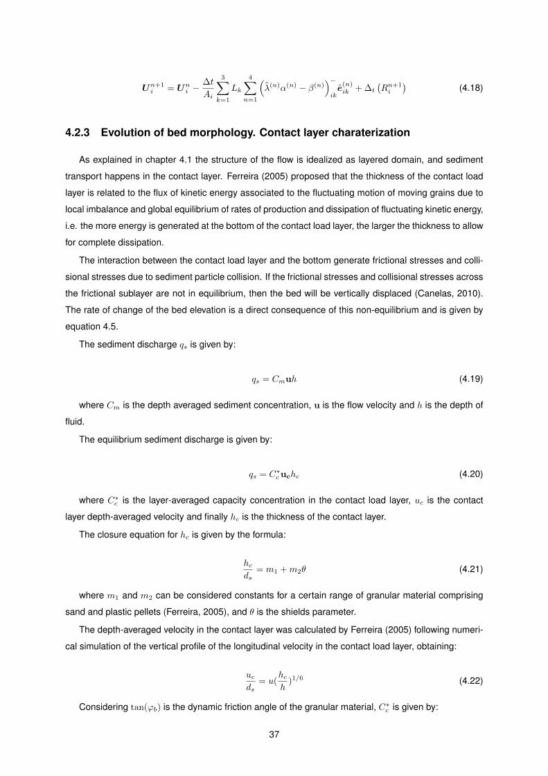
Un+1i = Un
i −∆t
Ai
3∑k=1
Lk
4∑n=1
(λ(n)α(n) − β(n)
)−ike
(n)ik + ∆t
(Rn+1i
)(4.18)
4.2.3 Evolution of bed morphology. Contact layer charaterization
As explained in chapter 4.1 the structure of the flow is idealized as layered domain, and sediment
transport happens in the contact layer. Ferreira (2005) proposed that the thickness of the contact load
layer is related to the flux of kinetic energy associated to the fluctuating motion of moving grains due to
local imbalance and global equilibrium of rates of production and dissipation of fluctuating kinetic energy,
i.e. the more energy is generated at the bottom of the contact load layer, the larger the thickness to allow
for complete dissipation.
The interaction between the contact load layer and the bottom generate frictional stresses and colli-
sional stresses due to sediment particle collision. If the frictional stresses and collisional stresses across
the frictional sublayer are not in equilibrium, then the bed will be vertically displaced (Canelas, 2010).
The rate of change of the bed elevation is a direct consequence of this non-equilibrium and is given by
equation 4.5.
The sediment discharge qs is given by:
qs = Cmuh (4.19)
where Cm is the depth averaged sediment concentration, u is the flow velocity and h is the depth of
fluid.
The equilibrium sediment discharge is given by:
qs = C∗cuchc (4.20)
where C∗c is the layer-averaged capacity concentration in the contact load layer, uc is the contact
layer depth-averaged velocity and finally hc is the thickness of the contact layer.
The closure equation for hc is given by the formula:
hcds
= m1 +m2θ (4.21)
where m1 and m2 can be considered constants for a certain range of granular material comprising
sand and plastic pellets (Ferreira, 2005), and θ is the shields parameter.
The depth-averaged velocity in the contact layer was calculated by Ferreira (2005) following numeri-
cal simulation of the vertical profile of the longitudinal velocity in the contact load layer, obtaining:
ucds
= u(hch
)1/6 (4.22)
Considering tan(ϕb) is the dynamic friction angle of the granular material, C∗c is given by:
37
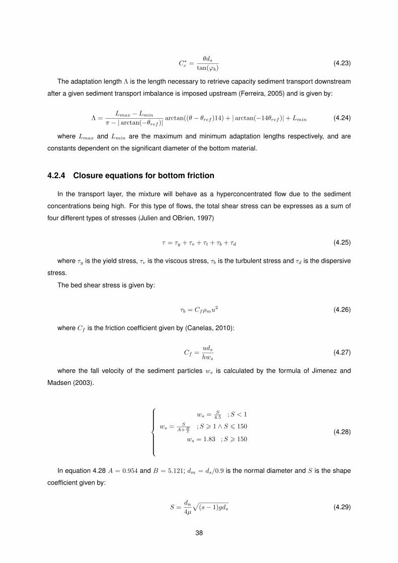
C∗c =θds
tan(ϕb)(4.23)
The adaptation length Λ is the length necessary to retrieve capacity sediment transport downstream
after a given sediment transport imbalance is imposed upstream (Ferreira, 2005) and is given by:
Λ =Lmax − Lmin
π − | arctan(−θref )|arctan((θ − θref )14) + | arctan(−14θref )|+ Lmin (4.24)
where Lmax and Lmin are the maximum and minimum adaptation lengths respectively, and are
constants dependent on the significant diameter of the bottom material.
4.2.4 Closure equations for bottom friction
In the transport layer, the mixture will behave as a hyperconcentrated flow due to the sediment
concentrations being high. For this type of flows, the total shear stress can be expresses as a sum of
four different types of stresses (Julien and OBrien, 1997)
τ = τy + τv + τt + τb + τd (4.25)
where τy is the yield stress, τv is the viscous stress, τb is the turbulent stress and τd is the dispersive
stress.
The bed shear stress is given by:
τb = Cfρmu2 (4.26)
where Cf is the friction coefficient given by (Canelas, 2010):
Cf =udshws
(4.27)
where the fall velocity of the sediment particles ws is calculated by the formula of Jimenez and
Madsen (2003).
ws = S4.5 ;S < 1
ws = SA+ B
S
;S > 1 ∧ S 6 150
ws = 1.83 ;S > 150(4.28)
In equation 4.28 A = 0.954 and B = 5.121; dm = ds/0.9 is the normal diameter and S is the shape
coefficient given by:
S =dn4µ
√(s− 1)gds (4.29)
38
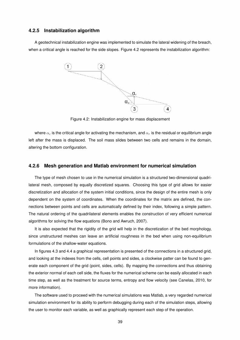
4.2.5 Instabilization algorithm
A geotechnical instabilization engine was implemented to simulate the lateral widening of the breach,
when a critical angle is reached for the side slopes. Figure 4.2 represents the instabilization algorithm:
Figure 4.2: Instabilization engine for mass displacement
where αc is the critical angle for activating the mechanism, and αr is the residual or equilibrium angle
left after the mass is displaced. The soil mass slides between two cells and remains in the domain,
altering the bottom configuration.
4.2.6 Mesh generation and Matlab environment for numerical simulation
The type of mesh chosen to use in the numerical simulation is a structured two-dimensional quadri-
lateral mesh, composed by equally discretized squares. Choosing this type of grid allows for easier
discretization and allocation of the system initial conditions, since the design of the entire mesh is only
dependent on the system of coordinates. When the coordinates for the matrix are defined, the con-
nections between points and cells are automatically defined by their index, following a simple pattern.
The natural ordering of the quadrilateral elements enables the construction of very efficient numerical
algorithms for solving the flow equations (Bono and Awruch, 2007).
It is also expected that the rigidity of the grid will help in the discretization of the bed morphology,
since unstructured meshes can leave an artificial roughness in the bed when using non-equilibrium
formulations of the shallow-water equations.
In figures 4.3 and 4.4 a graphical representation is presented of the connections in a structured grid,
and looking at the indexes from the cells, cell points and sides, a clockwise patter can be found to gen-
erate each component of the grid (point, sides, cells). By mapping the connections and thus obtaining
the exterior normal of each cell side, the fluxes for the numerical scheme can be easily allocated in each
time step, as well as the treatment for source terms, entropy and flow velocity (see Canelas, 2010, for
more information).
The software used to proceed with the numerical simulations was Matlab, a very regarded numerical
simulation environment for its ability to perform debugging during each of the simulation steps, allowing
the user to monitor each variable, as well as graphically represent each step of the operation.
39
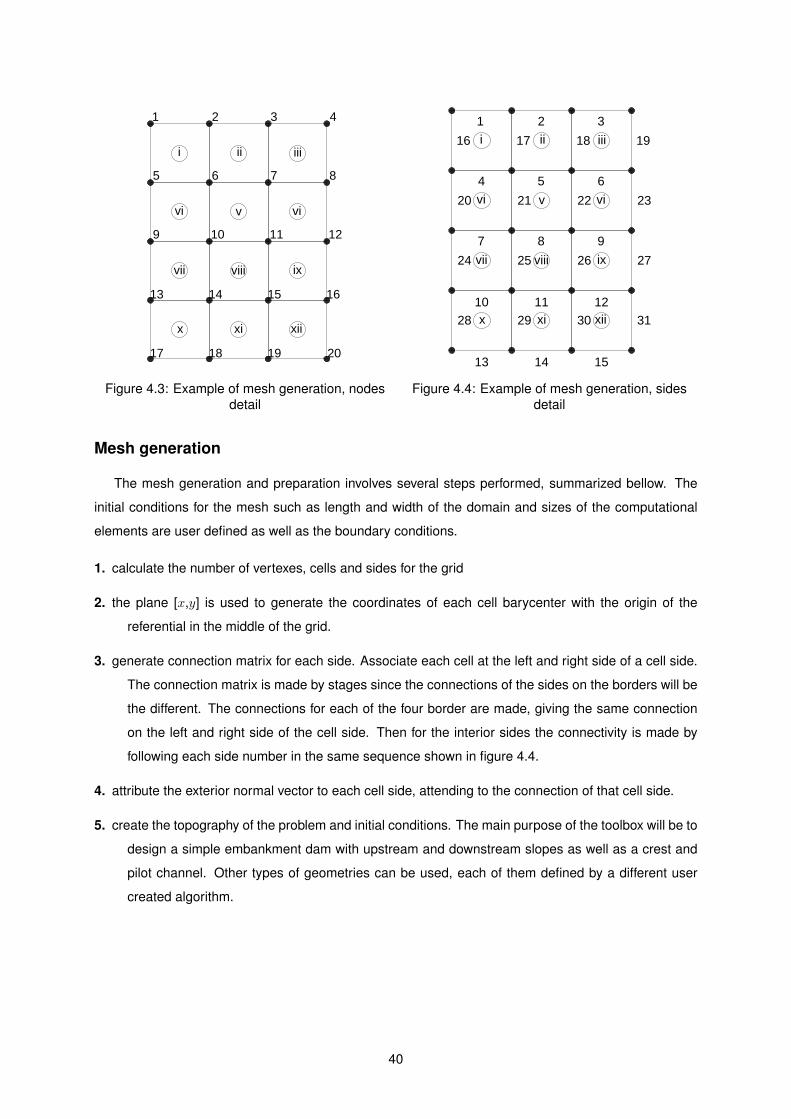
1 2 3
5 6 7
9 10 11
191817
13 14 15
i ii iii
vi v vi
vii viii ix
x xi xii
4
8
12
20
16
Figure 4.3: Example of mesh generation, nodesdetail
1
16
2 3
4 5 6
7 8 9
17 18
222120
24 25 26
302928
19
23
27
31
151413
10 11 12
i ii iii
vi v vi
vii viii ix
x xi xii
Figure 4.4: Example of mesh generation, sidesdetail
Mesh generation
The mesh generation and preparation involves several steps performed, summarized bellow. The
initial conditions for the mesh such as length and width of the domain and sizes of the computational
elements are user defined as well as the boundary conditions.
1. calculate the number of vertexes, cells and sides for the grid
2. the plane [x,y] is used to generate the coordinates of each cell barycenter with the origin of the
referential in the middle of the grid.
3. generate connection matrix for each side. Associate each cell at the left and right side of a cell side.
The connection matrix is made by stages since the connections of the sides on the borders will be
the different. The connections for each of the four border are made, giving the same connection
on the left and right side of the cell side. Then for the interior sides the connectivity is made by
following each side number in the same sequence shown in figure 4.4.
4. attribute the exterior normal vector to each cell side, attending to the connection of that cell side.
5. create the topography of the problem and initial conditions. The main purpose of the toolbox will be to
design a simple embankment dam with upstream and downstream slopes as well as a crest and
pilot channel. Other types of geometries can be used, each of them defined by a different user
created algorithm.
40

Chapter 5
Results
5.1 Introduction
5.2 Comparison between analytical solutions and numerical sim-
ulations
5.2.1 Dam-break test cases, initial conditions
For the dam-break test cases, the classical Stoker solution is presented and compared to the numer-
ical model, as well as other solutions for particular cases of the Stoker solution (dry bed, discontinuous
bottom elevation), with the intent to develop shocks and to verify the models ability to simulate the solu-
tion. The non-dimensional parameters that describe the initial conditions for the test cases must specify
all the dependent variables (Ferreira, 2005) are for this problem:
α =hR + |min(0, Ybl)|hL + |min(0, Ybl)|
; δ =Ybl
hL +max(0, Ybl)(5.1)
Figure 5.1 shows a the general scheme for the initial conditions when dealing with unidimensional
dam break test cases:
Figure 5.1: Initial conditions for 1D dam break test case
41
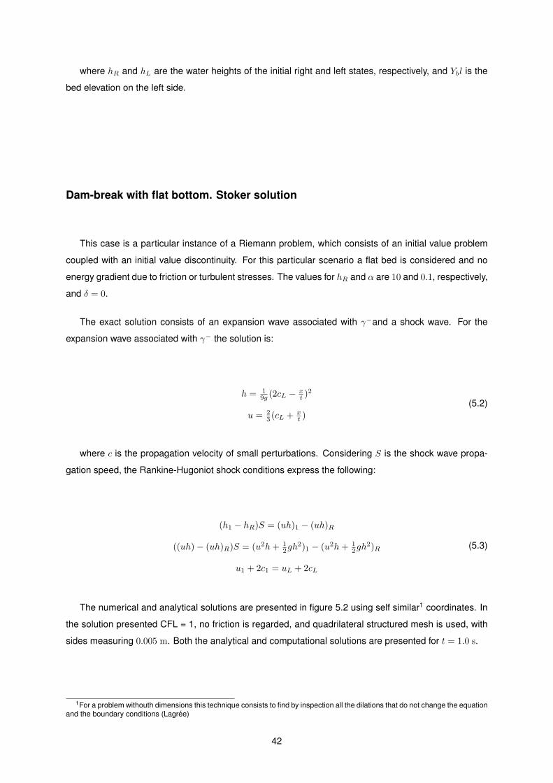
where hR and hL are the water heights of the initial right and left states, respectively, and Ybl is the
bed elevation on the left side.
Dam-break with flat bottom. Stoker solution
This case is a particular instance of a Riemann problem, which consists of an initial value problem
coupled with an initial value discontinuity. For this particular scenario a flat bed is considered and no
energy gradient due to friction or turbulent stresses. The values for hR and α are 10 and 0.1, respectively,
and δ = 0.
The exact solution consists of an expansion wave associated with γ−and a shock wave. For the
expansion wave associated with γ− the solution is:
h = 19g (2cL − x
t )2
u = 23 (cL + x
t )
(5.2)
where c is the propagation velocity of small perturbations. Considering S is the shock wave propa-
gation speed, the Rankine-Hugoniot shock conditions express the following:
(h1 − hR)S = (uh)1 − (uh)R
((uh)− (uh)R)S = (u2h+ 12gh
2)1 − (u2h+ 12gh
2)R
u1 + 2c1 = uL + 2cL
(5.3)
The numerical and analytical solutions are presented in figure 5.2 using self similar1 coordinates. In
the solution presented CFL = 1, no friction is regarded, and quadrilateral structured mesh is used, with
sides measuring 0.005 m. Both the analytical and computational solutions are presented for t = 1.0 s.
1For a problem withouth dimensions this technique consists to find by inspection all the dilations that do not change the equationand the boundary conditions (Lagree)
42

-2 -1.5 -1 -0.5 0 0.5 1 1.5 2
0
0.2
0.4
0.6
0.8
1
Z’=
z/h
L
-2 -1.5 -1 -0.5 0 0.5 1 1.5 2
0
0.2
0.4
0.6
0.8
1
X’ = (x/t)/(
gh)
U’=
u/h
L
Bottom elevation Water elevation h - exact solution Flow velocity u - exact solution
Figure 5.2: Comparison between analytical and numerical solution of the Stoker problem
Figure 5.2 shows a clearly the left moving expansion wave and right moving shock wave. The figure
also shows a good accordance between the computed and exact solution for the problem presented.
Dam-break with flat bottom. Ritter solution
The Ritter solution is a particular case for the Stoker solution, when hR = 0 i.e. in a dry bed scenario.
The solution for the shock wave speed expressed in 5.3 becomes:
limhR→0 S = limhR→0(uh)1−(uh)R
h1−hR= u1
limh1→0 u1 = limhR→0 2(cL − c1) = 2cL
(5.4)
therefore the solution becomes simple and is the expansion wave expressed, for which the profile is
given by equation 5.2.
For the the conditions hL = 10.0 m, α = 0.0, δ = 0.0 and CFL = 1.0, the solution is computed
against the analytical solution, with the same mesh used to compute the Stoker solution and the results
are shown in figure 5.3 for t = 1.0 s
43
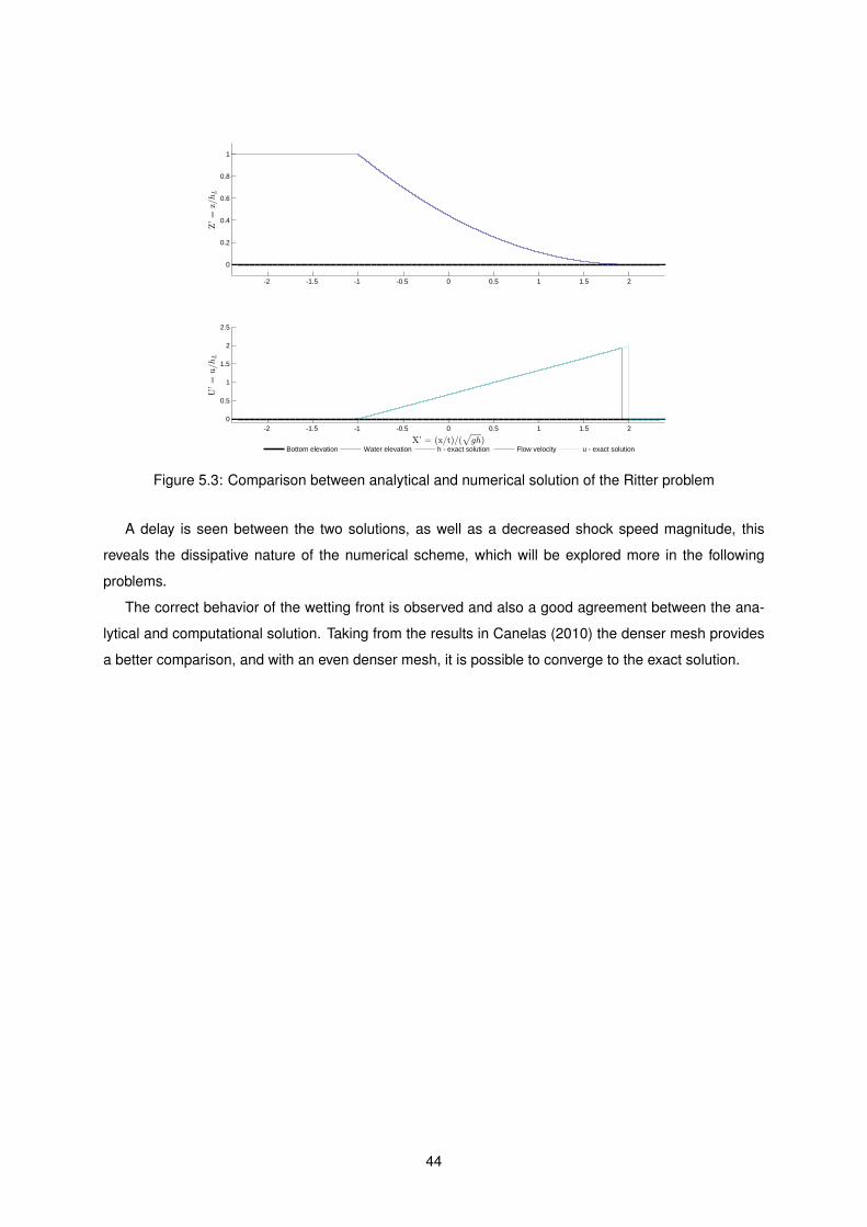
-2 -1.5 -1 -0.5 0 0.5 1 1.5 2
0
0.2
0.4
0.6
0.8
1
Z’=
z/h
L
-2 -1.5 -1 -0.5 0 0.5 1 1.5 20
0.5
1
1.5
2
2.5
X’ = (x/t)/(
gh)
U’=
u/h
L
Bottom elevation Water elevation h - exact solution Flow velocity u - exact solution
Figure 5.3: Comparison between analytical and numerical solution of the Ritter problem
A delay is seen between the two solutions, as well as a decreased shock speed magnitude, this
reveals the dissipative nature of the numerical scheme, which will be explored more in the following
problems.
The correct behavior of the wetting front is observed and also a good agreement between the ana-
lytical and computational solution. Taking from the results in Canelas (2010) the denser mesh provides
a better comparison, and with an even denser mesh, it is possible to converge to the exact solution.
44

5.2.2 2D test cases
In this section initial value problems are simulated and compared with the respective analytical so-
lutions. The first two are circular dam problems, which are a 2D generalization of the 1D dam break
problems presented before, and the solutions are the same since the 2D solution has radial symmetry
with the 1D solution.
Cirucular dam break. Dry bottom
The dry bottom circular dam break is also a radial generalization of the Ritter solution i.e. for a circular
water column with 1.0 m and α = 0, δ = 0.0 the exact solution is the same as for the unidimensional
case.
The numerical solution is presented in figure 5.4 in self similar coordinates, for a computational
domain of 20000× 20000 discretized as 100× 100 cells and CFL = 1.0.
-5 -4 -3 -2 -1 0 1 2 3 4 50
0.2
0.4
0.6
0.8
1
Z’=
z/h
max
-5 -4 -3 -2 -1 0 1 2 3 4 50
0.5
1
1.5
2
2.5
3
X’ = (x/t)/(
gh)
U’=
u/c
max
Bottom elevation Water elevation Flow velocity
Figure 5.4: Circular dam-break problem simulation for water and velocity profiles, t = 1s
Comparing the 2D and 1D solutions it is observed that the behavior is the same, as expected. The
numerical solution also shows the influence of the mesh density in the agreement between numerical
and analytical solutions since for the numerical scheme the velocity profile is smoother and the peak is
eliminated. For a denser mesh, the peak is more noticeable as show for the unidimensional case.
The 3D water profile and velocity map are also presented in figures 5.5 and 5.6 respectively
where the radial symmetry is observed. Inn the velocity magnitude field the effects of the orthogonal
mesh are also observed, in the form of velocity peaks in the principal directions x and y. These peaks
45

Figure 5.5: 3D perspective of the water profile, t = 1 s
Figure 5.6: 2D flow velocity map, t = 1 s
46

appear as a result of the structured quadrilateral mesh chosen to represent the domain, where the sides
of the cells are always parallel or perpendicular to the directions x and y of the referential.
5.2.3 Water movement in parabolic basin
The problems presented in the following section where proposed by Thacker (1981) and exact solu-
tions for different initial conditions where derived from the shallow water equations. The general formu-
lation of the problem is presented in Appendix A.
There are two particular cases for the geometry of the basin presented:
D = D0(1− x2
L2− y2
l2) (5.5)
where in equation 5.5, D0 is depth at the center of the basin, and L and l are the distance from the
center of the basin to the shoreline in the x and y direction respectively.
The first is for l = L rendering the basin a parabola of revolution, the other is for L l, creating
a cylindrical channel. Only the first particular case will be considered for the following solutions of the
nonlinear shallow-water wave equations.
Oscilations for which the surface remains planar
Assuming that for the general equations presented in equation A.6 and A.7, ux = uy = vx = vy = 0,
leading to hxx = hyy = hxy = hyx, only u0, v0 and h0 define the initial conditions of the motion. For
basins studied, consider f = 0.
Consider ω the frequency of the motion, the complete solution for the motion is (Thacker, 1981) :
u = −νω sin(ω1t); v = −νω cos(ω1t)
h = 2νD0
L ( xL cos(ω1t)− yL sin(ω1t)− ν
2L );
ω1 = ( 2gD0
L2 )2
(5.6)
where ν determines the amplitude of the motion.
The shoreline is determined by equation 5.7,
(x− ν cos(ω1t))2 + (y + ν sin(ω1t))
2 = L2 (5.7)
where the moving shoreline is a circle in the x, y plane and the motion is such that the center of the
circle orbits the center of the basin (Thacker, 1981).
The initial profile of the analytical solution is shown in figure 5.8 for t = T/8 and the full 3D domain is
presented in figure 5.7.
47
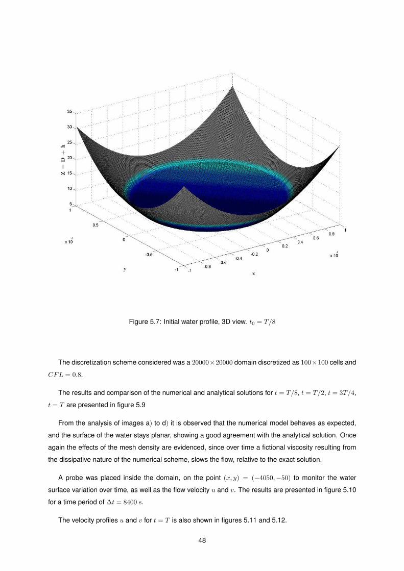
Figure 5.7: Initial water profile, 3D view. t0 = T/8
The discretization scheme considered was a 20000×20000 domain discretized as 100×100 cells and
CFL = 0.8.
The results and comparison of the numerical and analytical solutions for t = T/8, t = T/2, t = 3T/4,
t = T are presented in figure 5.9
From the analysis of images a) to d) it is observed that the numerical model behaves as expected,
and the surface of the water stays planar, showing a good agreement with the analytical solution. Once
again the effects of the mesh density are evidenced, since over time a fictional viscosity resulting from
the dissipative nature of the numerical scheme, slows the flow, relative to the exact solution.
A probe was placed inside the domain, on the point (x, y) = (−4050,−50) to monitor the water
surface variation over time, as well as the flow velocity u and v. The results are presented in figure 5.10
for a time period of ∆t = 8400 s.
The velocity profiles u and v for t = T is also shown in figures 5.11 and 5.12.
48

-1 -0.5 0 0.5 1x 10
4
0
2
4
6
8
10
12
14
16
Z=
D+
h(m
)
x (m)
water surface elevation basin floor
Figure 5.8: Initial water profile, 2D view. t0 = T/8
-1 -0.5 0 0.5 1x 10
4
0
2
4
6
8
10
12
14
16
Ele
vati
on
(m)
x (m)
D + h
a a)t = T/8
-1 -0.5 0 0.5 1x 10
4
0
2
4
6
8
10
12
14
16
Ele
vati
on
(m)
x (m)
D + h
b)t = T/2
-1 -0.5 0 0.5 1x 10
4
0
2
4
6
8
10
12
14
16
Ele
vati
on
(m)
x (m)
D + h
c)t = 3T/4
-1 -0.5 0 0.5 1x 10
4
0
2
4
6
8
10
12
14
16
Ele
vati
on
(m)
x (m)
D + h
d)t = T
Figure 5.9: Water surface elevation in different instants, comparison with analytical solution
Oscilations for which the surface is curved
Now assuming that u0 = v0 = 0, restricting the motion to convergence toward, divergence from, and
rotation about the center of the basin. For a this particular case,f = 0, hx = hy = 0, ux = vy and49

0 1000 2000 3000 4000 5000 6000 7000 8000 9000-1.5
-1
-0.5
0
0.5
1
1.5
velo
cit
y
time (s)
u v u - exact solution v - exact solution
Figure 5.10: Variation of u and v over time for probe 1 (x, y) = (−4050,−50). Comparison withanalytical solution
-1 -0.5 0 0.5 1x 10
4
-0.5
0
0.5
1
1.5
2
2.5
3
Flo
wvelo
city
x (m)
u
Figure 5.11: Longitudinal profile of u velocity field for t = 2200 s
uy = −vx, the seven initial conditions presented in Appendix A are reduced to three and are calculated
by equations 5.8
δ2ux
δt2 + ux8gD0L
2
+ 6uxδux
δt + 4ux3 = 0;
δvxδt + 2uxvx = 0;
δh0
δt + 2ux(h0 +D0) = 0
(5.8)
50

-1 -0.5 0 0.5 1x 10
4
-1.5
-1
-0.5
0
0.5
1
Flo
wvelo
city
x (m)
v
Figure 5.12: Longitudinal profile of v velocity field for t = 2200 s
the initial value of vx is vx0 and the inital value of h is ν. Considering that ux is initially zero, the
complete solution for the motion becomes (Thacker, 1981):
u = 11−A cos(ωt) [ 1
2ω(x)A sin(ωt) +A(cos(ωt)− 1)];
v = 11−A cos(ωt) [ 1
2ω(y)A sin(ωt) +A(cos(ωt)− 1)];
h = D0 (1−A2)12
1−A cos(ωt) − 1− x2+y2
L2 [ 1−A2
1−A cos(ωt) − 1].
(5.9)
where A is a constant that depends on values vx0 and ν and is calculated by equation 5.10:
A =(D0 + ν)2 −D0
2
(D0 + ν)2 +D02 (5.10)
the frequency of the motion ω is given by equation 5.11
ω2 =8gD0
L2; (5.11)
The initial profile of the water surface is a parabola of revolution and the profile is presented in figures
5.13 and 5.14 for the instant t = 0 s. The parameters used the same for the previous problem, and are
also expressed in table .....
51

Figure 5.13: Initial Water elevation, 3D view, t = 0
The motion of the water in the parabolic basin is such the shoreline is a circle with a variable radius
that expands and contracts as the central water elevation is above or beow the equilibrium level, creating
a convex or concave water surface respectively. This induces multiple wetting and drying situations
across the domain, providing a very good test for model stability under the conditions presented.
The analytical and numerical solutions for the motion are presented in figure 5.14 corresponding to
the instants t = 0, t = T/4, t = T/2, t = 3T/4.
where a good agreement between the analytical and numerical solutions is observed. It is also noted
that a the amplitude of the motion is dampened over time, due to the drying algorithm, which leaves a thin
layer of water in the domain, for model stability purposes (Kurganov and Petrova, 2008). This causes a
dissipation of the total momentum. Further analysis and remodeling of the wetting and drying algorithm
should be considered in order to preserve the total momentum.
The same problem is also evident when analyzing the data collected by the probes, placed at the
same locations as the previous problem. Probe data is presented in figure 5.15 for probe 1 and figure
5.15 for probe 2.
The dampening caused by the mesh induced viscosity is more noticeable for the velocity in the x
52
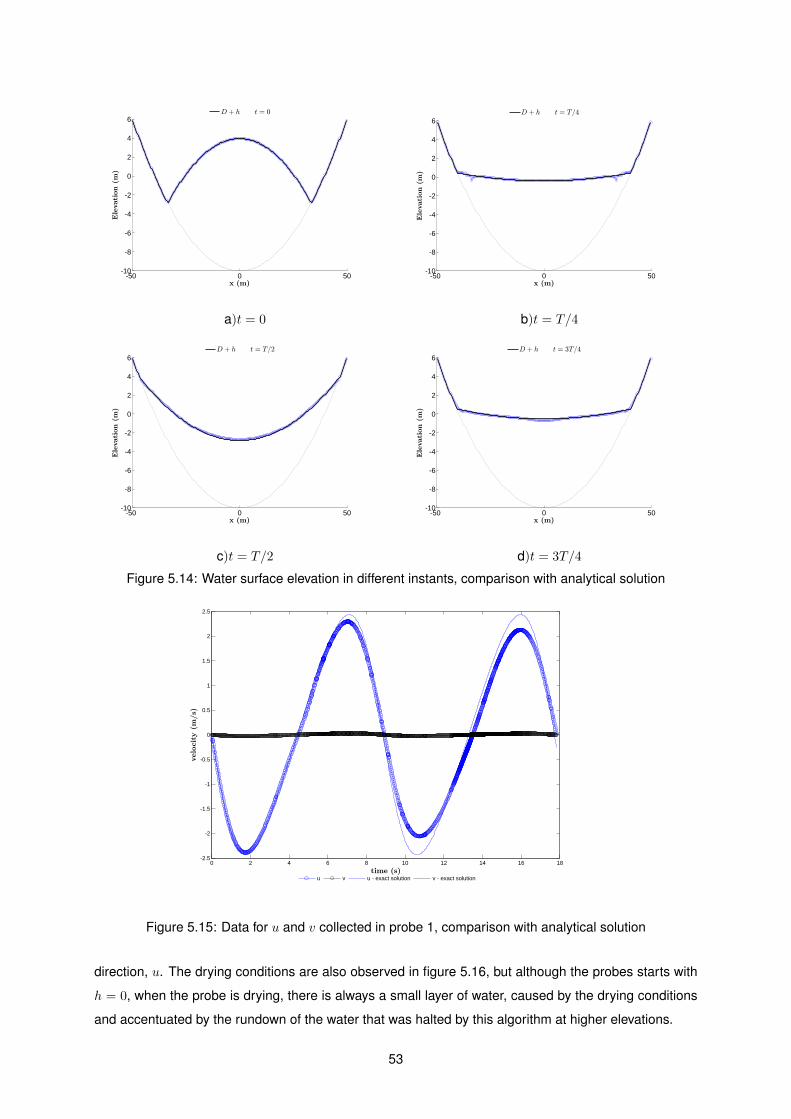
-50 0 50-10
-8
-6
-4
-2
0
2
4
6E
levati
on
(m)
x (m)
D + h t = 0
a)t = 0
-50 0 50-10
-8
-6
-4
-2
0
2
4
6
Ele
vati
on
(m)
x (m)
D + h t = T/4
b)t = T/4
-50 0 50-10
-8
-6
-4
-2
0
2
4
6
Ele
vati
on
(m)
x (m)
D + h t = T/2
c)t = T/2
-50 0 50-10
-8
-6
-4
-2
0
2
4
6
Ele
vati
on
(m)
x (m)
D + h t = 3T/4
d)t = 3T/4
Figure 5.14: Water surface elevation in different instants, comparison with analytical solution
0 2 4 6 8 10 12 14 16 18-2.5
-2
-1.5
-1
-0.5
0
0.5
1
1.5
2
2.5
velo
cit
y(m
/s)
time (s)
u v u - exact solution v - exact solution
Figure 5.15: Data for u and v collected in probe 1, comparison with analytical solution
direction, u. The drying conditions are also observed in figure 5.16, but although the probes starts with
h = 0, when the probe is drying, there is always a small layer of water, caused by the drying conditions
and accentuated by the rundown of the water that was halted by this algorithm at higher elevations.
53

0 2 4 6 8 10 12 14 16 18-5
-4
-3
-2
-1
0
1
2
3
4
5
velo
cit
y(m
/s)
time (s)
u v u - exact solution v - exact solution
Figure 5.16: Data for u and v collected in probe 2, comparison with analytical solution
To conclude the analysis of the drying conditions, a three dimensional map for the velocity in the x
direction is presented. Note that the velocity peaks of the velocity map correspond to cells where water
was previous stoped and is now flowing down the domain walls.
54

Figure 5.17: 3D view of the u velocity profile t = T
55

5.2.4 Mobile bed. Riemann problems
Initial conditions
The previous problems where developed to test model accuracy and stability in frictionless and non
erodible beds. The conceptual model features sediment mass conservation, and the purpose of the
numerical model is to simulate situations where dam breaching is expect, a phenomena characterized by
the complex erosion mechanisms as explained in chapter 2. The governing equations where presented
in chapter 4 and the following chapter will focus on some of the theoretical solutions for the Riemann
problem with the full set of equations of conservation for mass, momentum and sediment mass.
The problems are presented in the form of dam breaks, which can be idealized as instantaneous
removal of a vertical barrier initially separating two constant states that extend indefinitely on both up-
and downstream directions. If this description is valid, then the problem is a Riemann problem and
admits self-similar solutions if the system of governing hyperbolic equations is homogeneous (Ferreira,
2005).
Figure 5.18: Initial conditions for the Riemann problem posed to the geomorphic shallow waterequations
In figure 5.18 the initial conditions are presented.The variables, YL, YL, RR, RR, Y bL and Y bR are
the water elevation, the unit mass discharge and the bed elevation for the left (L) and right (R) constant
states separated by the initial discontinuity.
The solution of comprised of a combination of expansion and shock waves associated with the first
three characteristics γ1, γ2 and γ3 and the general structure of the solution is presented in figure 5.19.
Analytical solution for the Riemann problem
Two types of problem were considered, using the same non-dimensional parameters as in section
5.2.1. No flow resistance is considered to obtain the theoretical solution, and the sediment concentration
law is:
56

Figure 5.19: General wave structure of the Riemann solution for the geomorphic dam-break problem.
C = acu2h−1. (5.12)
where ac is the mobility coefficient. No flow resistance is considered to obtain the analytical solution.
The two different types of problem are presented in table 5.1 along with the initial conditions consid-
ered for each of the four problems analyzed.
Solution hL [m] hR [m] YbL [m] YbR [m] ac ds[m] s
0.40 0.00 0.00 0.00 0.0010142 0.003 1.5
0.40 0.00 0.00 0.10 0.0010142 0.003 1.5
0.40 0.10 0.08 0.00 0.0010142 0.003 1.5
0.40 0.10 0.00 0.08 0.0010142 0.003 1.5
Type A
Type B
Table 5.1: Initial conditions for the 2 types of solution for the geomorphic dam break problem
Solutions of type A problems are comprised of two rarefaction waves associated with γ(3) and γ(2)
and one shock wave associated with γ(1) characteristic. The 7× 7 system of equations the describe the
solution of the problem is:
(YR − Y1)S1 = (uh)R − (uh)1;
(RR −R1)S1 = (ρmu2h)R − (ρmu
2h)1 + g ∗ 12 ((ρmh
2)R − (ρmh2)1) + g ∗ 1
2 ((ρmh)R + (ρmh)1)(YbR − Yb1);
[((1− p)Yb + Ch)R − ((1− p)Yb + Ch)1]S1 = (Cuh)R − (Cuh)1
(5.13)
δuδh = fu
(2)(u1, h1);
δYb
δh = fz(2)(u1, h1);
(5.14)
57

δuδh = fu
(3)(u2, h2);
δYb
δh = fz(3)(u2, h2);
(5.15)
where C is the depth-averaged sediment concentration of the flow and ρm is the depth-averaged
volumetric mass of the flow, the index 1 and 2 indicate the corresponding constant states. Equations
5.14 and 5.15 are systems of 2 × 2 ODE’s the describe the expansion waves across the associated
characteristic. Equation 5.14 requires the boundary conditions u0 = uL, h0 = hL and Yb0 = YbL,
h0 = hL to the point h = h2
Solutions of type B problems feature a similar solution structure to Type A problems, but with a
shock wave associated with γ(2), and therefore must verify the Rankine-Hugoniot shock conditions, so
equations 5.14 are replaced by :
(Y1 − Y2)S2 = (uh)1 − (uh)2;
(R1 −R2)S2 = (ρmu2h)1 − (ρmu
2h)2 + g ∗ 12 ((ρmh
2)1 − (ρmh2)2) + g ∗ 1
2 ((ρmh)1 + (ρmh)2)(Yb1 − Yb2);
[((1− p)Yb + Ch)1 − ((1− p)Yb + Ch)2]S2 = (Cuh)1 − (Cuh)2
(5.16)
The analytical solutions Type A problems are presented in figures 5.20 and 5.21.
Figure 5.20: Analytical solution for Type A - problem 1
The 2 expansion waves associated with the γ(3) and γ(2) characteristics appear well defined and
separated by a constant state downstream of the negative expansion wave. The shock wave is also
presented, although almost negligible due to the dry initial state of the bed, which is a similar response
to the Ritter solution. The bed profile responds to the variations of the water profile.
58

Figure 5.21: Analytical solution for Type A - problem 2
Analytical solutions for problems of Type B are also presented in figures 5.22 and 5.23.
Figure 5.22: Analytical solution for Type B - problem 3
Figure 5.23: Analytical solution for Type B - problem 4.
As expected the solutions admit a shock wave associated to the γ(1) with a velocity higher than the
shock associated with the γ(2) characteristics field, thus verifying the RH shock conditions.
59

Comparison between numerical and analytical solutions
The numerical solutions were obtained for the same conditions as the analytical solution, i.e. featur-
ing no flow resistance, and a the same sediment discharge law. The adaptation length was taken suf-
ficiently small to ensure a quasi-equilibrium state for sediment continuity, but with an adaptation length
higher than the mesh size to ensure model stability.
For Type A problems the comparison between numerical and analytical solutions are presented in
figures 5.24 and 5.25. Problems 1 and 2 feature CFL = 0.9 and for t = 1 s. Problem 1 was simulated
with a 0.05× 0.05 mesh and Problem 2 with a 0.005× 0.005 mesh.
Figure 5.24: Results for numerical simulation of Problem 1, solution for water surface and bottomelevation and velocity profile. Comparison with analytical solution
Figure 5.25: Results for numerical simulation of Problem 2, solution for water surface and bottomelevation and velocity profile. Comparison with analytical solution
Analysis of the simulations shows that erosion levels have similar magnitudes, and the bottom evolu-
tion is in good agreement with the analytical solution. The shock induced by the bottom source terms is
inevitable at the end of the negative expansion wave (Ferreira et al., 2006). The numerical scheme has
difficulties in simulating the wave front. The simulations provided are a good simulation of the complex
dam break problem.
For the type B problems, numerical and analytical solutions are presented in figures 5.24 and 5.25.
Problems 3 and 4 feature CFL = 0.9 and for t = 1 s. Problem 3 was simulated with a 0.05× 0.05 mesh
60
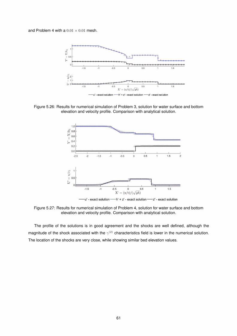
and Problem 4 with a 0.01× 0.01 mesh.
Figure 5.26: Results for numerical simulation of Problem 3, solution for water surface and bottomelevation and velocity profile. Comparison with analytical solution.
Figure 5.27: Results for numerical simulation of Problem 4, solution for water surface and bottomelevation and velocity profile. Comparison with analytical solution.
The profile of the solutions is in good agreement and the shocks are well defined, although the
magnitude of the shock associated with the γ(2) characteristics field is lower in the numerical solution.
The location of the shocks are very close, while showing similar bed elevation values.
61

5.2.5 Simulation of dam breach and comparison with experimental work
The main goal of this work is to provide a numerical model capable of simulating the breaching of
embankment dams, hence, a simulation of the experimental work is now presented and the results from
both the numerical model and experiments are compared. The model is equipped with an instabilization
engine, applied in similar way than the ones showed in chapter 2.2. This is a very simple approach to the
complex physics involved in the sliding failure that occurs during the breaching process, and for future
work, a more complex instabilization engine should be developed.
Simulation results and comparison
A simplified version of the dam presented in the experiments is now modeled and the breaching is
simulated. The simulated embankment features similar characteristics to the embankment used in trial
2, and this parameters are presented in table 5.2
Table 5.2: Numerical model, embankment characteristics
The 3D rendering of the dam is also presented in figure 5.28
Figure 5.28: Numerical model, embankment geometry
The domain is composed of W = 10 × L = 10 cm cells. The water that flow trough the breach is
collected at a reservoir downstream, and the water is put back in the domain, upstream of the breaching
zone, distributed over an are, as to not disturb the area near the breach.
The final breaching hydrograph is then obtained and compared with the one from trial 2, and the
comparison is presented in figure 5.29:
62

1600 1800 2000 2200 2400 2600 2800 3000-0.1
0
0.1
0.2
0.3
0.4
0.5
0.6
0.7
Time [s]
Q [m
3/s]
Numerical model Weighted average Flowmeter Simple Average Probe R6
Figure 5.29: Comparison between numerical and experimental outflow hydrographs for trial 2
The peak discharge is able to be reached for the numerical model, and the evolution of the discharge
is similar do the experimental results, showing a good agreement between numerical and experimental
work, for very similar embankment characteristics. Note that the hydrograph evolution is smoother,
because the instabilization engine does not consider sudden breach enlargements, and thus it takes
longer to reach the peak. This confirms the need for further work and development of a geotechnical
instabilization algorithm that can reproduce the sliding of mass due to undercutting.
Figure 5.31 shows a comparison of an upstream view of the breaching process for the experiments
and for the numerical model.
The images show that the model can simulate the breaching process of an earth dam. There is also
clear influence of the mesh detail, although the mesh size was chosen for computational efficiency, since
a more detailed mesh would lead to infeasible computational times.
To note that the instabilization algorithm can in fact reproduce a collapse of the breach sides, but in a
very different way than the observed in the experiments. The collapse is taken as an interaction between
two cells, and it is clear from the image analysis that the mass displacement should not be a sequential
event, and should be modeled in a more complex way.
The bottom elevations for 2 time frames of the breaching process are presented in figures 5.32 and
5.33.
The bottom profile in the numerical model shows a good agreement with the observed in the ex-
periment. It is noticeable that more definition is needed in the proximity of the breach for a better
characterization of the bottom evolution.
The water surface contours are presented for the same instant in figures 5.34 and 5.35
Similarities are evident on both water surface maps and the same definition problem is posed, but
despite this the water elevation is in good agreement with the experimental data as the water profile
63
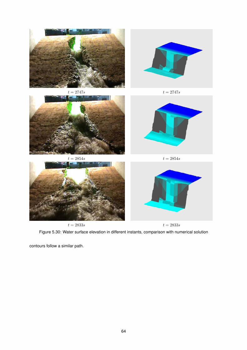
t = 2747s t = 2747s
t = 2854s t = 2854s
t = 2833s t = 2833s
Figure 5.30: Water surface elevation in different instants, comparison with numerical solution
contours follow a similar path.
64

t = 2961s t = 2961s
t = 3017s t = 3017s
Figure 5.31: Water surface elevation in different instants, comparison with analytical solution
-1.2
-1.0
-0.8
-0.6
-0.4
-0.22
1.8
1.6
1.4
1.2
1
0.8
0.6
0
0.1
0.2
0.3
0.4
0.5
Downstream distance [m]Distance along the crest [m]
z[m
]
Figure 5.32: Bottom elevation for the upstream view of the embankment, numerical model.
65

Figure 5.33: Bottom elevation for the upstream view of the embankment, experiment 2
0.440.445
0.45
0.4550.460.4
6
0.465
0.465
0.47
0.47
0.4750.475
0.4750.48
0.48
0.48
0.48
0.485
0.485
0.485
0.485
0.49
0.49 0.490.49
Coordinate x [m]
Coord
inat
ey
[m]
-1.2 -1.0 -0.8 -0.6 -0.4 -0.31
0.9
0.8
0.7
0.6
0.44 0.45 0.46 0.47 0.48 0.49Water elevation [m]
Figure 5.34: Water Surface contours for the simulation of experiment 2.
Figure 5.35: Water Surface contours for experiment 2.
66

Chapter 6
Conclusions
In this work, an effort to simulate the breaching process of dams was undertaken. A numerical
model was developed using a simple high-level language, MATLAB, meant to become the core of a
toolbox. It is envisaged that a dam-breach MATLAB toolbox would be subjected to a wide interest in the
water resources community thus contributing to advance the confidence of users in deterministic tools
to estimate breach hydrographs.
The conservation equations are essentially the shallow water equations complemented with mass
conservation equations and a bed morphology equation. The model features non-equilibrium sediment
transport. The closure equations were taken from existing literature on fluvial transport and sheet-flow
(intense bedload transport) studies. The discretization method, drawn from previous studies Canelas
et al. (2013), is fully conservative, robust and obeys C-property.
The model, named STAVBreach, as a upgraded installment of the model used by Canelas et al.
(2011), was validated with one-dimensional and two-dimensional solutions of the shallow water equa-
tions with and without sediment transport. The agreement between the simulations and the theoretical
results was satisfactory. In particular, the conservation equations proved to be able to describe the water
movement and the bed configuration for several well-known cases with analytical solutions.
However, some problems were detected, mostly in the numerical discretization approach. The prob-
lems proposed by Thacker for water movement in parabolic basins with flat and curved surfaces posed
some difficulties on the simulations, due to the multiple wetting and drying fronts, as well as evident
mesh rigidity observed. The Riemann problems consisting of geomorphic dam breaks with variations
on the water level and bottom elevations revealed that the numerical scheme has trouble simulating the
shock waves celerity and propagation as well as defining the constant state due to the non-equilibrium
nature of the sediment transport equations used. The scheme was confirmed to be somewhat dissi-
pative. Additionally some problems were in what concerns the rigidity imposed by the quadrangular
mesh.
Experiments conducted at a medium-scale laboratory facility at LNEC provided data for a more
complex validation phase. Outflow hydrographs, determined from two different methods, were obtained
as well as data for characterization of the breaching process.
67
The instabilization conceptual model employed to describe the mass detachment phenomena ob-
served at the banks of the pilot channel proved to be satisfactory but not ideal. The enlargement os
the breach sides was correctly modeled but with artificial values of geotechnical parameters. It is clear
that the instabilization phenomena needs to be described with more detail, namely with the inclusion of
three-dimensional phenomena such as undercutting, in order to be able to simulate the sudden breach
enlargements observed in the experiments.
6.1 Future Work
Some recommendations and ideas for future work are proposed in this chapter:
- The is still work to be done in implementing the code as a MATLAB toolbox in order for it to be
used effectively but end users.
- A revision of the numerical scheme is needed, and a higher order scheme should be developed in
order to avoid excessive numerical diffusion;
- Further analysis and validation of the geotechnical instabilization model should be done, consid-
ering coupling with, well known and well studied slope instabilization numerical models, whenever
possible.
- An alternative wetting and drying algorithm should be considered to mitigate the effects that current
one has, especially when drying occurs in steep slopes.
- The model is explicit and heavily dependent on problem scale for computational efficiency, so for
the future, graphical processing of the data should be implemented to improve simulation efficiency
in order to simulate large periods of time in detailed domains.
- Different structured cells should be experimented since the square orthogonal mesh was able to
simulate the problems without a significant loss of detail, and a much larger gain of efficiency, if
coupled with some suggestions already made.
- Pre- and post-processing to become a proper toolbox for MATLAB.
- Include coding for GPU to improve computational performance, again to become a MATLAB tool-
box.
68
Bibliography
Alonso, E. (2004). Suelos compactados en la teoria y en la pratica.
Alonso, E. and N. Pinyol (2008). Unsaturated soil mechanics in earth and rockfill dam engineering. In
D. . G. . Toll, C. . E. . Augarde, D. . Gallipoli, and S. . J. . Wheeler (Eds.), Proceedings of the 1st
European Conference, E-UNSAT 2008. Taylor and Francis Group.
A.M. Bento, et al. (2014). Quantification of the breach hydrograph of homogeneous dams subjected to
overtopping.
ASTM. D698. standard test methods for laboratory compaction characteristics of soil using standard
effort 12 400 ft-lbf/ft3 600 kn-m/m3. west conshohocken (pa): Astm international; 2011.
Bono, G. and A. M. Awruch (2007). Numerical study between structured and unstructured meshes for
Euler and Navier-Stokes Equations. Mecanica computacional Vol XXVI.
Caldeira, L. (2001). Curso de exploracao e seguranca de barragens. Instituto da Agua.
Canelas, R. (2010). 2D Mathematical Modeling of Discontinuous Shallow Sediment-laden Flows. Ph. D.
thesis, Instituto Superior Tecnico.
Canelas, R., J. Murillo, and R. Ferreira (2011). 2d simulation of discontinuous shallow flows. In Experi-
mental Methods in Hydraulic Research, pp. 141–153. Springer.
Canelas, R., J. Murillo, and R. M. Ferreira (2013). Two-dimensional depth-averaged modelling of dam-
break flows over mobile beds. Journal of Hydraulic Research 51(4), 392–407.
Cardoso, R. (2010). Earth fill works. Instituto Superior Tecnico.
Emelen, S. V., Y. Zech, and S. Soares-Frazao (2015). Impact of sediment transport formulations on
breaching modelling. Journal of Hydraulic Research 53(1), 60 – 72.
Ferreira, R. M., S. Amaral, J. Leal, and B. Spinewine (2006). Discontinuities in geomorphic dam-break
flows. In J. L. R.M.L. Ferreira, E. Alves and A. Cardoso (Eds.), River Flow 2006, Volume 2, pp.
1521–1530. Taylor and Fancis Group.
Ferreira, R. M. L. (2005). River Morphodynamics and Sediment Transport - Conceptual Model and
Solutions. Ph. D. thesis, Instituto Superior Tecnico.
69

Guan, M., N. G. Wright, and P. A. Sleigh (2014). 2d process-based morphodynamic model for flooding
by noncohesive dyke breach. Journal of Hydraulic Engineering 140(7).
INC., M. (2011). Soil Compaction Handbook. P.O.Box 6524, Carson, CA 90749: MULTIQUIP INC.
Jimenez, J. A. and O. S. Madsen (2003). A simple formula to estimate settling velocity of natural sedi-
ments. Journal of Waterway, Port, Coastal, and Ocean Engineering 129(2), 70–78.
Julien, P. and J. OBrien (1997). On the importance of mud and debris flow rheology in structural design.
In C. L. Chen (Ed.), Debris-Flow Hazards Mitigation: Mechanics, Prediction and Assessment. ASCE.
Kurganov, A. and G. Petrova (2008). A central-upwind scheme for nonlinear water waves generated
by submarine landslides. In Hyperbolic Problems: Theory, Numerics, Applications, pp. 635–642.
Springer.
Lagree, P. Self similar solutions.
Marcelino, J. (2008). Projecto, construcao e exploracao de pequenas barragens de aterro. LNEC.
Murillo, J. and P. Garcıa-Navarro (2010). Weak solutions for partial differential equations with source
terms: application to the shallow water equations. Journal of Computational Physics 229(11), 4327–
4368.
Narita, K. (2000). Design and construction of embankment dams. Aichi Institute of Technology.
NEVES, E. d. (2002). Algumas consideracoes sobre a mecanica de enrocamentos. Solos e Rochas,
Revista Latino-Americana de Geotecnia, ABMS/ABGE 25(3), 161–203.
Parra, M. A. and J. C. C. Barranco (2003). Dams from the roman era in spain: analysis of design forms.
In Proceedings of the First International Congress on Construction History: Madrid, 20th-24th january
2003, pp. 243–257. Instituto Juan de Herrera.
Pickert, G., G. H. Jirka, A. Bieberstein, and J. Brauns (2004). Experiments on overtopped homogeneous
embankments: Soil/water interactions and breach development. In Proc. Int. Conf. - Disasters and
Society - From Hazard Assessment to Risk Reduction. Karlsruhe.
Pickert, G., V. Weitbrecht, and A. Bieberstein (2011). Breaching of overtopped non-cohesive river em-
bankment controlled by apparent cohesion. Journal of Hydraulic Research 4, 143 – 156.
RSB (2007). Regulamento de seguranca de barragens.
Santos, J. (2015). Experimental investigation of failure by overtopping of homogeneous earth dams.
Master’s thesis, Instituto Superior Tecnico.
Silva, S. (2001). Dams: What They Are and What They Do.
Singh, V. P. (1996). Dam Breach Modeling Technology, Volume 17 of Water Science and Technology
Library. Kluwer Academic Publishers.
70
Spinewine, B., A. Delobbe, L. Elslander, and Y. Zech (2004). Experimental investigation of the breach
growth process in sand dikes. In Proceedings of the River Flow 2004, pp. 983–991. Taylor and Francis
Group.
Swartenbroekx, C., S. Soares-Frazao, R. Staquet, and Y. Zech (2010). Two-dimensional operator for
bank failures induced by water-level rise in dam-break flows. Journal of Hydraulic Research 48(3),
302–314.
Thacker, W. C. (1981). Some exact solutions to the nonlinear shallow-water wave equations. Journal of
Fluid Mechanics 107, 499 – 508.
Toro, E. (2001). Shock-Capturing Methods for Free Surface Shallow Flows. Wiley.
Volz, C., P. Rousselot, D. Vetsch, R. Mueller, R. Faeh, and R. Boes (2010). Numerical modeling of
dam breaching processes due to overtopping flow. In Proceedings of the 8th ICOLD European Club
symposium, pp. 691–696. Innsbruck,.
Zhao, G., Y. Ren, P. J. Visser, and W. S. J. Uijttewaal (2013). Flow process of the embankment breaching.
In Proceedings of 2013 IAHR World Congress.
71

72

Appendix A
Water movement in parabolic basins,
general formulation
In case an appendix if deemed necessary, the document cannot exceed a total of 100 pages...
Some definitions and vector identities are listed in the section below.
A.1 General case
The formulation of the shallow water wave equations in shallow basins is the following:
δuδt + u δuδx + v δuδy − fv + g δhδx = 0;
δuδt + u δvδx + v δvδy + fu+ g δhδy = 0;
δuδt + δ
δx [u(D + h)] + δδy [v(D + h)] = 0.
(A.1)
In A.1 the first 2 equations describe the the variation of the velocity components u and v, and the
third equations is the continuity equation. f is the Coriolis parameters which accounts for the earth’s
rotation and g is the gravity acceleration.
The approach taken was to assume the existence of solutions for u and v in the form:
u = u0 + uxx+ uyy; v = v0 + vxx+ vyy. (A.2)
requiring the solution for h to have the following form:
h = h0 + hxx+ hyy +1
2hxxx
2 +1
2hyyy
2 +1
2(hxy + hxyx)xy; (A.3)
The surface elevation ,h, is positive if it is above the equilibrium level, and the depth function D is
positive bellow the same equilibrium level. Therefore D + h is the total depth of water.
To satisfy the continuity equation the depth function is described by equation A.4:
73

D = D0(1− x2
L2− y2
l2). (A.4)
so that the basin is an elliptical paraboloid. The equilibrium shoreline is determined by D = 0 and is
the ellipse described by equation A.5
x2
L2+y2
l2= 1. (A.5)
The time dependent coefficients in equationsA.2, A.3 and A.4, u0, ux, uy, v0, vx, vy and h0 must
vanish in order to satisfy the continuity equation, thus the coefficients described are required to satisfy
the following equations:
δh0
δt + (ux + vy)(D0 + h0) + u0hx + v0hy = 0;
δhx
δt + (2ux + vy)hx + vxhy + u0(hxx − 2D0
L2 ) + v0hxy = 0;
δhy
δt + (2vy + ux)hy + uyhx + v0(hyy − 2D0
l2 ) + u0hxy = 0;
δhxx
δt + (3ux + vy)(hxx − 2D0
L2 ) + 2vxhxy = 0;
δhyy
δt + (3vy + ux)(hyy − 2D0
l2 ) + 2uyhxy = 0;
δhxy
δt + 2(ux + vy)hxy + uy(hxx − 2D0
L2 ) + vx(hyy − 2D0
l2 ) = 0.
(A.6)
The six equations plus the requirement that hxy = hyx which leads to:
δ
δt(vx − uy) + (ux + vy)(vx − uy + f) = 0; (A.7)
12 initial conditions total are needed, corresponding to the initial values of u0, ux, uy, v0, vx, vy, h0,
hx, hy, hxx, hyy and hxy, which fully define the initial fields u, v, h.
74

Appendix B
Compaction of experimental
embankments. Control and Execution
B.1 Compaction procedure
1 - Mix the soil to promote homogeneity in the mixture and to break apart lumps of soil and clay;
2 - Remove obvious big rocks from the soil;
3 - Clean the embankment site with water to promote adherence of the first layer of the embankment;
5 - Drop the soil consistently in a single location and then spread, this promotes uniformity of the layer
and does not have a compaction action on the soil. Remove any rocks or lumps of clay if there are
any;
6 - Layer height = 15 cm;
7 - Switch on the compaction plate;
· switch the ignition button on;
· pull the string to turn the motor on;
· switch off the ignition button;
· Select the frequency of the vibratory plate;
8 - Pass the compaction plate in a straight line along the length of the embankment at a steady;
pace(similar to the executed in the test embankments). Avoid stepping on parts of the embankment
that have yet to be compacted;
9 - Repeat step 8 until the number of passes has been achieved;
10 - Do the compaction control using a non invasive test after half the embankment design height has
been reached.
75

B.2 Trial embankments
Trial embankments are made to test compaction techniques and equipments, and its results at a
small scale and reduced cost, without acting on the design embankment. In the experiments trial em-
bankments where made to draw the compaction curve of the compaction plate by varying the number
of passes and keeping the water content in the soi- The trial embankment was composed of 2 layers.
The first layer measuring 5 cm is a retreading layer so the concrete does no influence the compaction
technique. The second layer measured 15 cm, corresponding to the layer height used in the design
embankment. The process is demonstrated in figure B.1
a) b)
c)
d)
Figure B.1: Trial embankment construction process (a) ; b) ; c)) and sand bottle test (d))
Controled variables. Results
The variables monitored using the trial embankments where the number of passes with the com-
paction plate, the speed of the passing and the frequency of the vibratory plate.
Figure B.2 shows the resulting compaction curves for 1, 3 and 6 passes with the equipment.
76

1,950
2,000
2,050
2,100
2,150
2,200
PE
SO V
OL
ÚM
ICO
SE
CO
(g/
cm3)
PROCTOR
PROCTOR CORRIGIDO
Vib. 1
Vib. 3
Vib. 6
1,800
1,850
1,900
4 5 6 7 8 9 10 11 12 13 14 15 16 17 18
TEOR EM ÁGUA (%)
Figure B.2: Grain size distribution curve. Exterior of the soil bank.
77
Related Documents