Dept. of Applied Mathematics Univ. of Crete Numerical methods for shallow water waves – 1 / 60 Numerical methods for shallow water wave equations Th. Katsaounis Dept. of Applied Math. Univ. of Crete, IACM, FORTH, Crete, GREECE Supported by ACMAC project EU-FP7 joint work with A. Delis TUC, Greece

Welcome message from author
This document is posted to help you gain knowledge. Please leave a comment to let me know what you think about it! Share it to your friends and learn new things together.
Transcript

Dept. of Applied Mathematics Univ. of Crete Numerical methods for shallow water waves – 1 / 60
Numerical methodsfor
shallow water wave equations
Th. Katsaounis
Dept. of Applied Math. Univ. of Crete,IACM, FORTH, Crete, GREECE
Supported by ACMAC project EU-FP7
joint work withA. Delis TUC, Greece
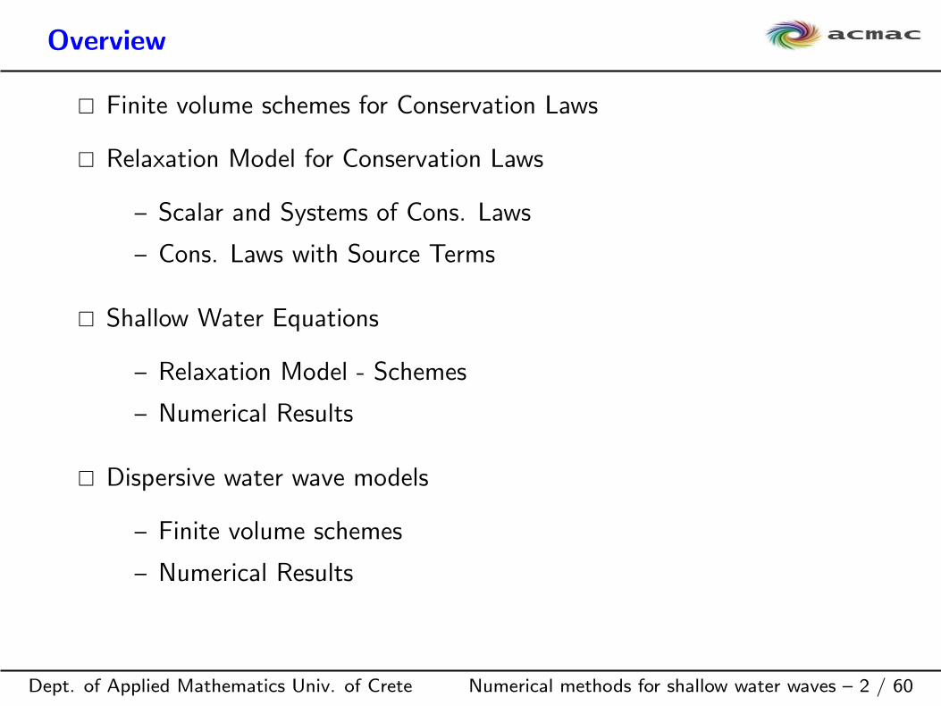
Overview
Dept. of Applied Mathematics Univ. of Crete Numerical methods for shallow water waves – 2 / 60
Finite volume schemes for Conservation Laws
Relaxation Model for Conservation Laws
– Scalar and Systems of Cons. Laws
– Cons. Laws with Source Terms
Shallow Water Equations
– Relaxation Model - Schemes
– Numerical Results
Dispersive water wave models
– Finite volume schemes
– Numerical Results
Finite volume schemes for Conservation Laws
Dept. of Applied Mathematics Univ. of Crete Numerical methods for shallow water waves – 3 / 60
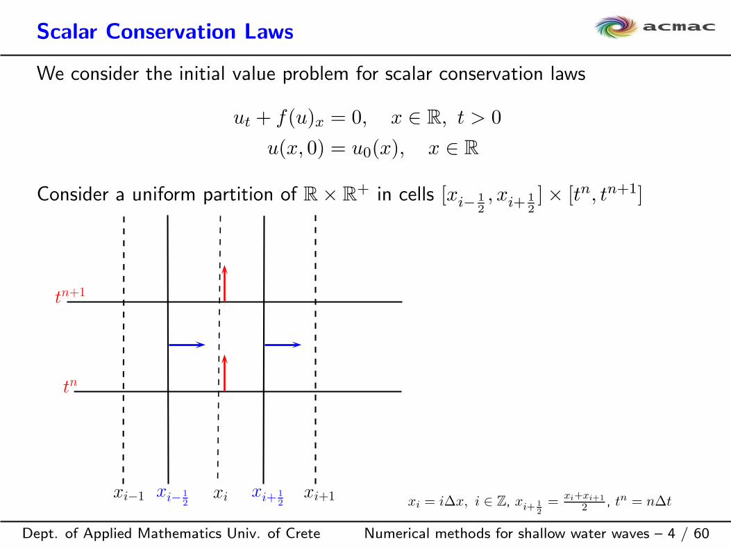
Scalar Conservation Laws
Dept. of Applied Mathematics Univ. of Crete Numerical methods for shallow water waves – 4 / 60
We consider the initial value problem for scalar conservation laws
ut + f(u)x = 0, x ∈ R, t > 0
u(x, 0) = u0(x), x ∈ R
Consider a uniform partition of R× R+ in cells [xi− 1
2
, xi+ 1
2
]× [tn, tn+1]
xi− 1
2
xi+ 1
2
tn
tn+1
xi−1 xi xi+1 xi = i∆x, i ∈ Z, xi+ 1
2
=xi+xi+1
2 , tn = n∆t

Dept. of Applied Mathematics Univ. of Crete Numerical methods for shallow water waves – 5 / 60
0 =
∫ tn+1
tn
∫ xi+1
2
xi− 1
2
[ut + f(u)x] dx dt
=
∫ xi+1
2
xi− 1
2
[u(x, tn+1)− u(x, tn)
]dx+
∫ tn+1
tn
[f(u(xi+ 1
2
, t))− f(u(xi− 1
2
, t))]dt
= Change of Mass+ Difference of Fluxes in cell [xi− 1
2
, xi+ 1
2
]× [tn, tn+1]
Uni ∼ 1
∆x
∫ xi+1
2
xi− 1
2
u(x, tn)dx, Fni+ 1
2
:= F (U+,ni , U−,n
i+1 ) ∼1
∆t
∫ tn+1
tnf(u(xi+ 1
2
, t))dt
Uni approximates the average of u in Ci = [xi− 1
2
, xi+ 1
2
] at time tn
Fni+ 1
2
approximates the average in [tn, tn+1] at x = xi+ 1
2
F is a numerical flux functionU+,ni some approximation of u(xi+ 1
2
− 0, tn)
U−,ni+1 some approximation of u(xi+ 1
2
+ 0, tn)

Basic FV scheme
Dept. of Applied Mathematics Univ. of Crete Numerical methods for shallow water waves – 6 / 60
Un+1i = Un
i − ∆t
∆x
(Fni+ 1
2
− Fni− 1
2
)
F numerical flux function:
1. Consistency : F (u, u) = f(u)
2. Monotonicity : ∂uF > 0, ∂vF < 0
3. Upwind, Lax-Friedrichs, Lax-Wendroff, Godunov, Central, Roe’s, ...
CFL condition : supu |f ′(u)|∆t∆x ≤ 1
U+i , U−
i+1 ? Reconstruction process :
1. Piecewise constants : U+i = Ui, U−
i+1 = Ui+1
2. Piecewise linear : U+i = Ui +
∆x2 Si, U−
i+1 = Ui+1 − ∆x2 Si+1 where
Si ∼ ux(xi+ 1
2
), x ∈ Ci Si+1 ∼ ux(xi+ 1
2
), x ∈ Ci+1. Limiters.
3. Higher order polynomials are constructed using the cell averages Ui.
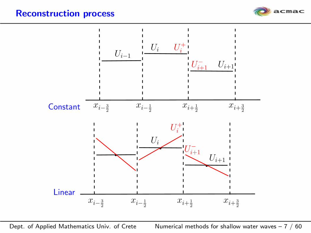
Reconstruction process
Dept. of Applied Mathematics Univ. of Crete Numerical methods for shallow water waves – 7 / 60
Constant xi− 3
2
xi− 1
2
xi+ 1
2
xi+ 3
2
Ui−1Ui U
+i
Ui+1U−i+1
Linear
b
b
b
xi− 3
2
xi− 1
2
xi+ 1
2
xi+ 3
2
Ui
U+i
Ui+1
U−i+1
Relaxation model for Conservation Laws
Dept. of Applied Mathematics Univ. of Crete Numerical methods for shallow water waves – 8 / 60

Relaxation Model for Scalar CL
Dept. of Applied Mathematics Univ. of Crete Numerical methods for shallow water waves – 9 / 60
ut + f(u)x = 0, x ∈ R, t > 0,
u(x, 0) = u0(x), x ∈ R.(1)
Relaxation system proposed by Jin & Xin 1995
ut + vx = 0,
vt + c2ux = −1
ǫ(v − f(u)), ǫ → 0
(2)
This system can be viewed as a regularization of (1) by the wave operator
ut + f(u)x = −ǫ(utt − c2uxx) +O(ǫ2).
Applying the Champan-Enskog expansion we get
ut + f(u)x = ǫ∂x((c2 − f ′(u)2
)∂xu
)+O(ǫ2).
If the subcharacteristic condition : |f ′(u)| < c holds then a rigorousconvergence analysis, for 1D scalar case, can be applied yielding at therelaxation limit ǫ → 0 the conservation law (1). (JX, 1995)
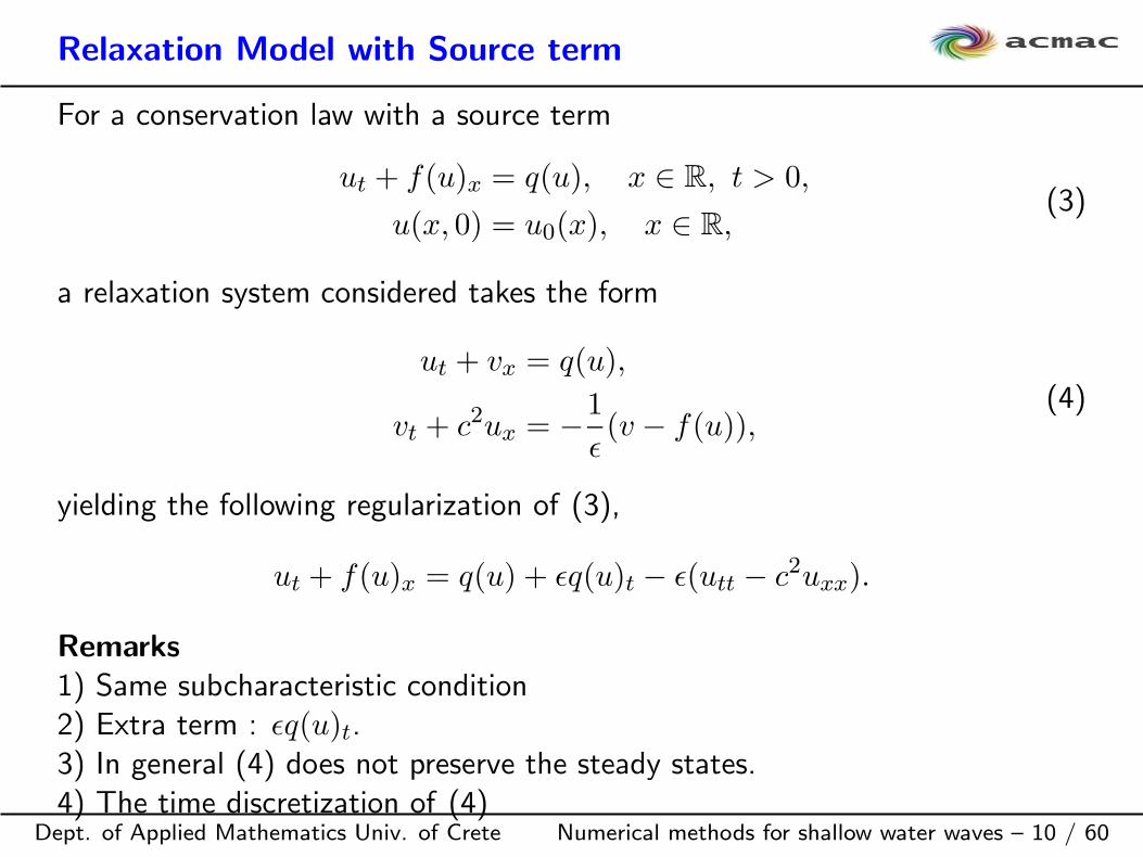
Relaxation Model with Source term
Dept. of Applied Mathematics Univ. of Crete Numerical methods for shallow water waves – 10 / 60
For a conservation law with a source term
ut + f(u)x = q(u), x ∈ R, t > 0,
u(x, 0) = u0(x), x ∈ R,(3)
a relaxation system considered takes the form
ut + vx = q(u),
vt + c2ux = −1
ǫ(v − f(u)),
(4)
yielding the following regularization of (3),
ut + f(u)x = q(u) + ǫq(u)t − ǫ(utt − c2uxx).
Remarks1) Same subcharacteristic condition2) Extra term : ǫq(u)t.3) In general (4) does not preserve the steady states.4) The time discretization of (4)

Dept. of Applied Mathematics Univ. of Crete Numerical methods for shallow water waves – 11 / 60
Un+1 − Un
∆t+ V n
x = q(Un+1),
V n+1 − V n
∆t+ c2Un
x = −1
ǫ(V n+1 − f(Un+1)),
(5)
is fully coupled system, not the case for the corresponding time discetizationof (2).An alternative approach : we consider the following relaxation system
ut + vx = 0,
vt + c2ux = −1
ǫ(v − f(u))− 1
ǫR(u),
(6)
where R(u) is an antiderivative of q(u),
R(u(x)) =
∫ x
q(u(s))ds .
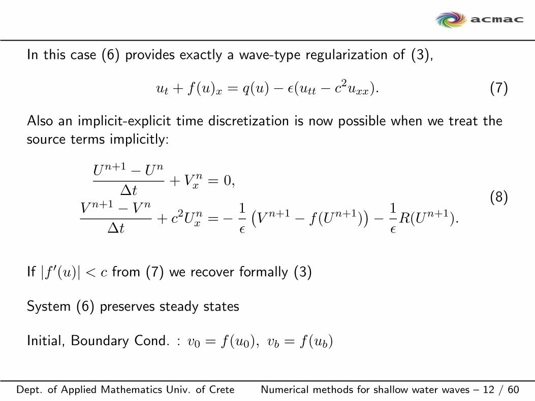
Dept. of Applied Mathematics Univ. of Crete Numerical methods for shallow water waves – 12 / 60
In this case (6) provides exactly a wave-type regularization of (3),
ut + f(u)x = q(u)− ǫ(utt − c2uxx). (7)
Also an implicit-explicit time discretization is now possible when we treat thesource terms implicitly:
Un+1 − Un
∆t+ V n
x = 0,
V n+1 − V n
∆t+ c2Un
x =− 1
ǫ
(V n+1 − f(Un+1)
)− 1
ǫR(Un+1).
(8)
If |f ′(u)| < c from (7) we recover formally (3)
System (6) preserves steady states
Initial, Boundary Cond. : v0 = f(u0), vb = f(ub)

System of CL
Dept. of Applied Mathematics Univ. of Crete Numerical methods for shallow water waves – 13 / 60
∂tu+d∑
j=1
∂xjFj(u) = 0, x ∈ R
d, u = u(x, t) ∈ Rn, t > 0
u(·, 0) = u0(·)
Relaxation model
∂tu+d∑
j=1
∂xjvj = 0,
∂tvi +Ai∂xiu = −1
ǫ(vi − Fi(u)) , i = 1, . . . , d
it’s a regularization by a wave operator of order ǫ, and Ai are symmetricpositive definite matrices with constant coefficients that are selected to satisfythe corresponding sub-characteristic conditions.

Shalllow Water Equations (SWE)
Dept. of Applied Mathematics Univ. of Crete Numerical methods for shallow water waves – 14 / 60

Shallow water eqns (1D)
Dept. of Applied Mathematics Univ. of Crete Numerical methods for shallow water waves – 15 / 60
ht + (hu)x = 0,
(hu)t + (hu2 +g
2h2)x = −ghZ ′,
(9)
General steady states :Q = hu = Cnst u2
2 + g(h+ Z) = CnstSWE is a hyperbolic system with source term
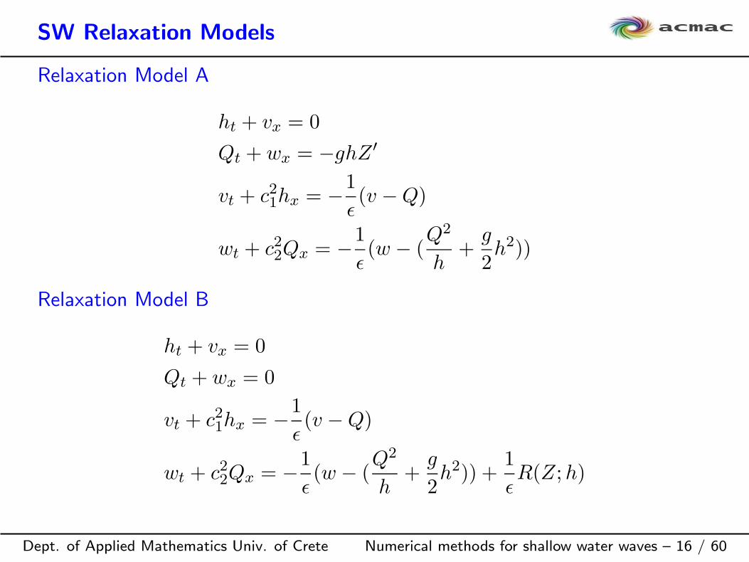
SW Relaxation Models
Dept. of Applied Mathematics Univ. of Crete Numerical methods for shallow water waves – 16 / 60
Relaxation Model A
ht + vx = 0
Qt + wx = −ghZ ′
vt + c21hx = −1
ǫ(v −Q)
wt + c22Qx = −1
ǫ(w − (
Q2
h+
g
2h2))
Relaxation Model B
ht + vx = 0
Qt + wx = 0
vt + c21hx = −1
ǫ(v −Q)
wt + c22Qx = −1
ǫ(w − (
Q2
h+
g
2h2)) +
1
ǫR(Z;h)

Dept. of Applied Mathematics Univ. of Crete Numerical methods for shallow water waves – 17 / 60
R(Z;h)(x) =
∫ x
g(hZ ′)(y)dy
c1, c2 are chosen according to sub-characteristic condition :
|λi(F′)| < ci, i = 1, 2, F ′ = Jacobian of flux vector
For Z ≡ 0, (A) ≡ (B)
For ǫ → 0 we recover the original SW system
Both relaxation systems have linear principal part
Implicit-explicit time discretizations for (B)
System (B) have same steady states as the continuous problem
Dept. of Applied Mathematics Univ. of Crete Numerical methods for shallow water waves – 18 / 60
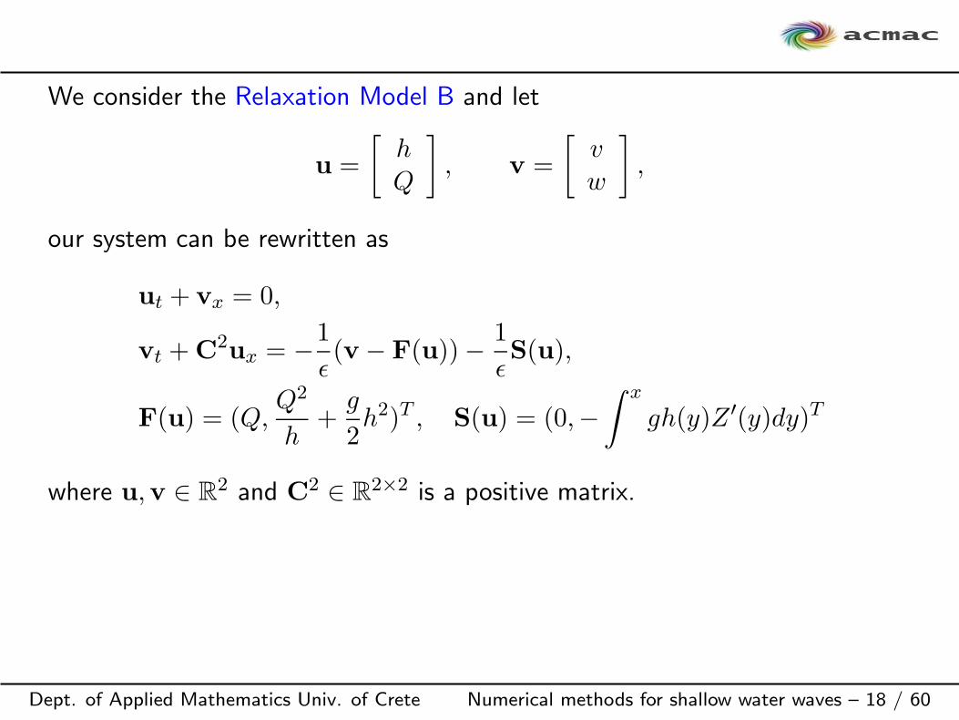
We consider the Relaxation Model B and let
u =
[hQ
], v =
[vw
],
our system can be rewritten as
ut + vx = 0,
vt +C2ux = −1
ǫ(v − F(u))− 1
ǫS(u),
F(u) = (Q,Q2
h+
g
2h2)T , S(u) = (0,−
∫ x
gh(y)Z ′(y)dy)T
where u,v ∈ R2 and C
2 ∈ R2×2 is a positive matrix.
Relaxation Schemes for SWE (1D)
Dept. of Applied Mathematics Univ. of Crete Numerical methods for shallow water waves – 19 / 60
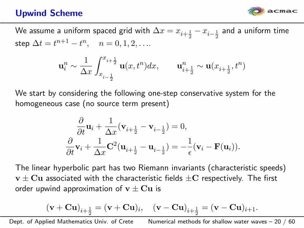
Upwind Scheme
Dept. of Applied Mathematics Univ. of Crete Numerical methods for shallow water waves – 20 / 60
We assume a uniform spaced grid with ∆x = xi+ 1
2
− xi− 1
2
and a uniform time
step ∆t = tn+1 − tn, n = 0, 1, 2, . . ..
uni ∼ 1
∆x
∫ xi+1
2
xi− 1
2
u(x, tn)dx, uni+ 1
2
∼ u(xi+ 1
2
, tn)
We start by considering the following one-step conservative system for thehomogeneous case (no source term present)
∂
∂tui +
1
∆x(vi+ 1
2
− vi− 1
2
) = 0,
∂
∂tvi +
1
∆xC
2(ui+ 1
2
− ui− 1
2
) = −1
ǫ(vi − F(ui)).
The linear hyperbolic part has two Riemann invariants (characteristic speeds)v ±Cu associated with the characteristic fields ±C respectively. The firstorder upwind approximation of v ±Cu is
(v +Cu)i+ 1
2
= (v +Cu)i, (v −Cu)i+ 1
2
= (v −Cu)i+1.
Dept. of Applied Mathematics Univ. of Crete Numerical methods for shallow water waves – 21 / 60
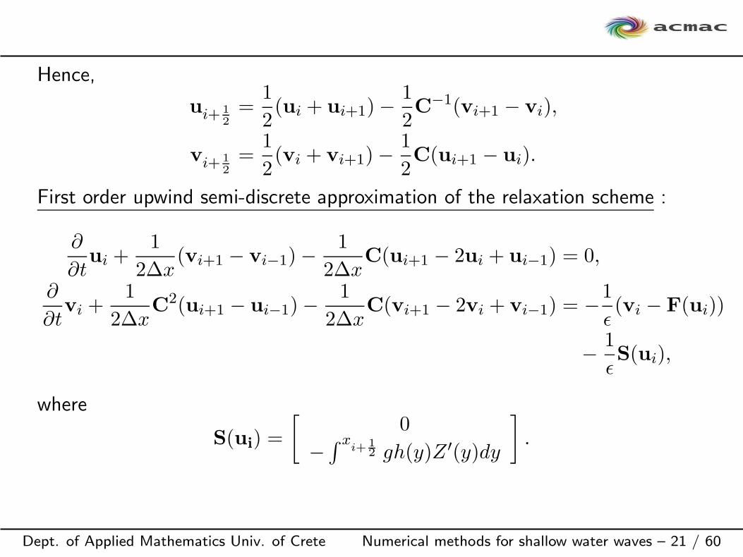
Hence,
ui+ 1
2
=1
2(ui + ui+1)−
1
2C
−1(vi+1 − vi),
vi+ 1
2
=1
2(vi + vi+1)−
1
2C(ui+1 − ui).
First order upwind semi-discrete approximation of the relaxation scheme :
∂
∂tui +
1
2∆x(vi+1 − vi−1)−
1
2∆xC(ui+1 − 2ui + ui−1) = 0,
∂
∂tvi +
1
2∆xC
2(ui+1 − ui−1)−1
2∆xC(vi+1 − 2vi + vi−1) = −1
ǫ(vi − F(ui))
− 1
ǫS(ui),
where
S(ui) =
[0
−∫ x
i+12 gh(y)Z ′(y)dy
].
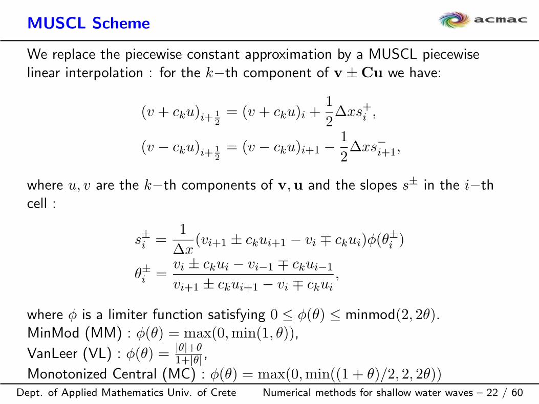
MUSCL Scheme
Dept. of Applied Mathematics Univ. of Crete Numerical methods for shallow water waves – 22 / 60
We replace the piecewise constant approximation by a MUSCL piecewiselinear interpolation : for the k−th component of v ±Cu we have:
(v + cku)i+ 1
2
= (v + cku)i +1
2∆xs+i ,
(v − cku)i+ 1
2
= (v − cku)i+1 −1
2∆xs−i+1,
where u, v are the k−th components of v,u and the slopes s± in the i−thcell :
s±i =1
∆x(vi+1 ± ckui+1 − vi ∓ ckui)φ(θ
±i )
θ±i =vi ± ckui − vi−1 ∓ ckui−1
vi+1 ± ckui+1 − vi ∓ ckui,
where φ is a limiter function satisfying 0 ≤ φ(θ) ≤ minmod(2, 2θ).MinMod (MM) : φ(θ) = max(0,min(1, θ)),
VanLeer (VL) : φ(θ) = |θ|+θ1+|θ| ,
Monotonized Central (MC) : φ(θ) = max(0,min((1 + θ)/2, 2, 2θ))
Dept. of Applied Mathematics Univ. of Crete Numerical methods for shallow water waves – 23 / 60
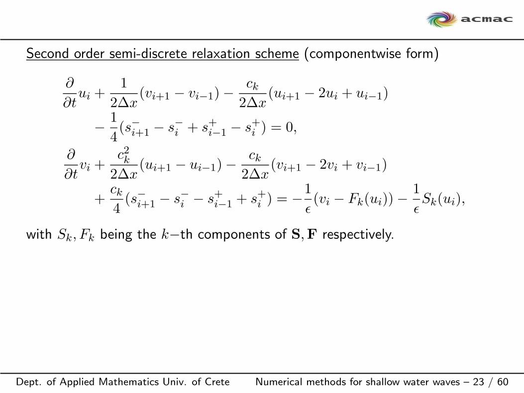
Second order semi-discrete relaxation scheme (componentwise form)
∂
∂tui +
1
2∆x(vi+1 − vi−1)−
ck2∆x
(ui+1 − 2ui + ui−1)
− 1
4(s−i+1 − s−i + s+i−1 − s+i ) = 0,
∂
∂tvi +
c2k2∆x
(ui+1 − ui−1)−ck
2∆x(vi+1 − 2vi + vi−1)
+ck4(s−i+1 − s−i − s+i−1 + s+i ) = −1
ǫ(vi − Fk(ui))−
1
ǫSk(ui),
with Sk, Fk being the k−th components of S,F respectively.
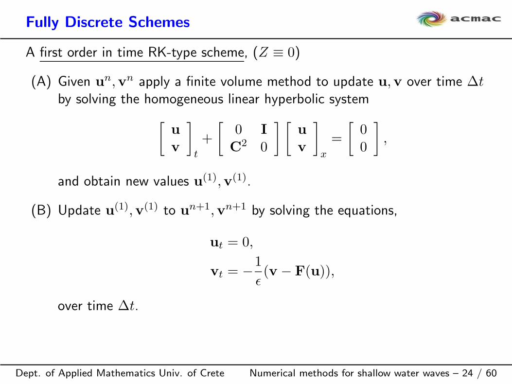
Fully Discrete Schemes
Dept. of Applied Mathematics Univ. of Crete Numerical methods for shallow water waves – 24 / 60
A first order in time RK-type scheme, (Z ≡ 0)
(A) Given un,vn apply a finite volume method to update u,v over time ∆t
by solving the homogeneous linear hyperbolic system
[u
v
]
t
+
[0 I
C2 0
] [u
v
]
x
=
[00
],
and obtain new values u(1),v(1).
(B) Update u(1),v(1) to u
n+1,vn+1 by solving the equations,
ut = 0,
vt = −1
ǫ(v − F(u)),
over time ∆t.
Dept. of Applied Mathematics Univ. of Crete Numerical methods for shallow water waves – 25 / 60
A second order in time RK-type scheme,
un,1 = u
n, vn,1 = v
n +∆t
ǫ(vn,1 − F(un,1)) +
∆t
ǫS(un,1);
u(1) = u
n,1 −∆tD+vn,1, v
(1) = vn,1 −∆tC2D+u
n,1;
un,2 = u
(1),
vn,2 = v
(1) − ∆t
ǫ(vn,2 − F(un,2))− 2∆t
ǫ(vn,1 − F(un,1))
− ∆t
ǫS(un,2)− 2∆t
ǫS(un,1);
u(2) = u
n,2 −∆tD+vn,2, v
(2) = vn,2 −∆tC2D+u
n,2;
un+1 =
1
2(un + u
(2)), vn+1 =
1
2(vn + v
(2)).
where
D+wi =1
∆x(wi+ 1
2
−wi− 1
2
).
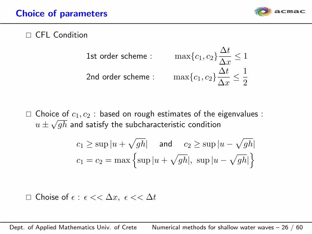
Choice of parameters
Dept. of Applied Mathematics Univ. of Crete Numerical methods for shallow water waves – 26 / 60
CFL Condition
1st order scheme : maxc1, c2∆t
∆x≤ 1
2nd order scheme : maxc1, c2∆t
∆x≤ 1
2
Choice of c1, c2 : based on rough estimates of the eigenvalues :u±
√gh and satisfy the subcharacteristic condition
c1 ≥ sup |u+√
gh| and c2 ≥ sup |u−√
gh|
c1 = c2 = maxsup |u+
√gh|, sup |u−
√gh|
Choise of ǫ : ǫ << ∆x, ǫ << ∆t
SWE(1D) : Numerical Results
Dept. of Applied Mathematics Univ. of Crete Numerical methods for shallow water waves – 27 / 60
No source term : Z ≡ 0: Dam Break problem
– Subcritical, supercritical, strongly supercritical
– Dry bed problem
Source term : Z 6= 0 :
– Flow at Rest
– Nontrivial Steady States
– Drain on Non-Flat bottom
Dam Break Flow Z ≡ 0
Dept. of Applied Mathematics Univ. of Crete Numerical methods for shallow water waves – 28 / 60
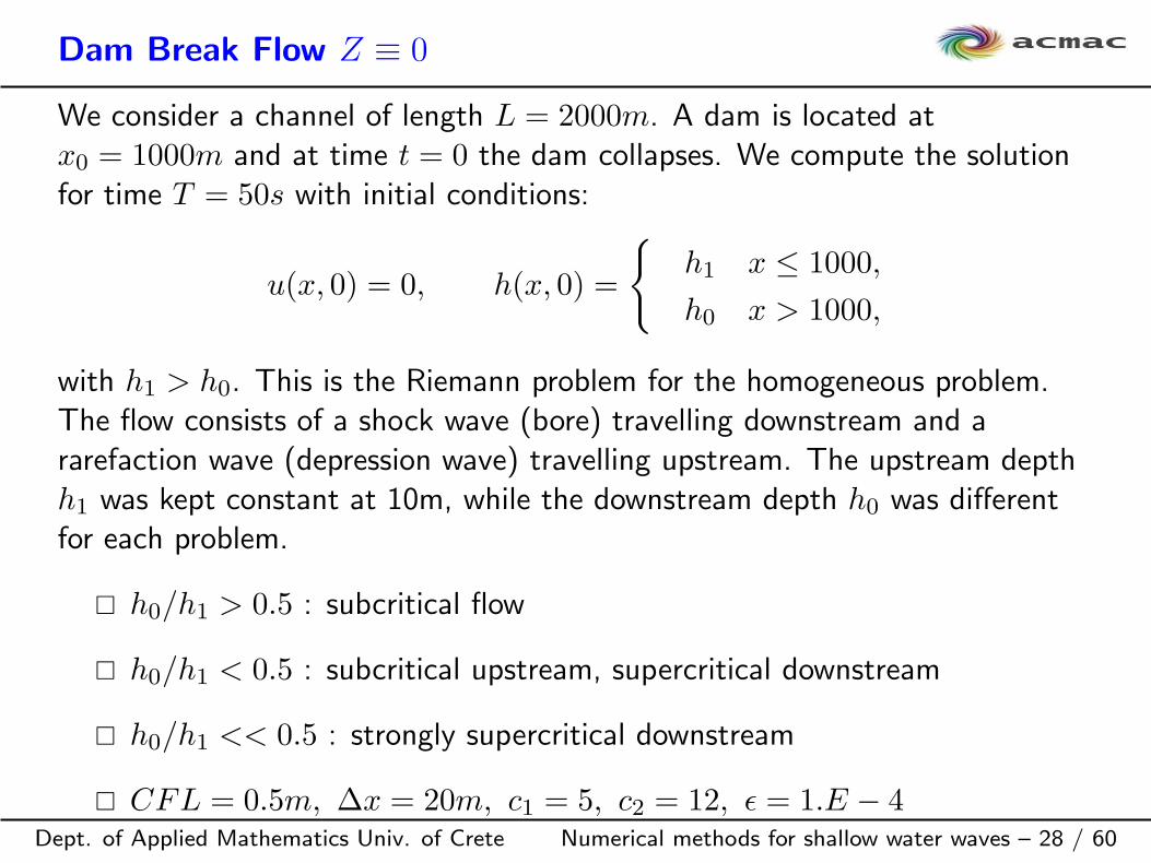
We consider a channel of length L = 2000m. A dam is located atx0 = 1000m and at time t = 0 the dam collapses. We compute the solutionfor time T = 50s with initial conditions:
u(x, 0) = 0, h(x, 0) =
h1 x ≤ 1000,
h0 x > 1000,
with h1 > h0. This is the Riemann problem for the homogeneous problem.The flow consists of a shock wave (bore) travelling downstream and ararefaction wave (depression wave) travelling upstream. The upstream depthh1 was kept constant at 10m, while the downstream depth h0 was differentfor each problem.
h0/h1 > 0.5 : subcritical flow
h0/h1 < 0.5 : subcritical upstream, supercritical downstream
h0/h1 << 0.5 : strongly supercritical downstream
CFL = 0.5m, ∆x = 20m, c1 = 5, c2 = 12, ǫ = 1.E − 4
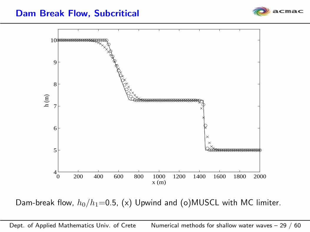
Dam Break Flow, Subcritical
Dept. of Applied Mathematics Univ. of Crete Numerical methods for shallow water waves – 29 / 60
0 200 400 600 800 1000 1200 1400 1600 1800 20004
5
6
7
8
9
10h
(m)
x (m)
Dam-break flow, h0/h1=0.5, (x) Upwind and (o)MUSCL with MC limiter.
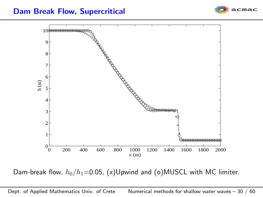
Dam Break Flow, Supercritical
Dept. of Applied Mathematics Univ. of Crete Numerical methods for shallow water waves – 30 / 60
0 200 400 600 800 1000 1200 1400 1600 1800 20000
1
2
3
4
5
6
7
8
9
10
h (m
)
x (m)
Dam-break flow, h0/h1=0.05, (x)Upwind and (o)MUSCL with MC limiter.
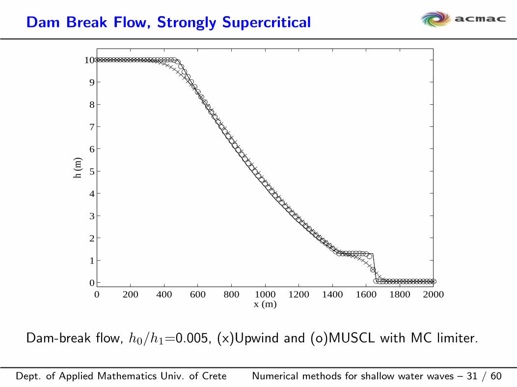
Dam Break Flow, Strongly Supercritical
Dept. of Applied Mathematics Univ. of Crete Numerical methods for shallow water waves – 31 / 60
0 200 400 600 800 1000 1200 1400 1600 1800 20000
1
2
3
4
5
6
7
8
9
10
h (m
)
x (m)
Dam-break flow, h0/h1=0.005, (x)Upwind and (o)MUSCL with MC limiter.
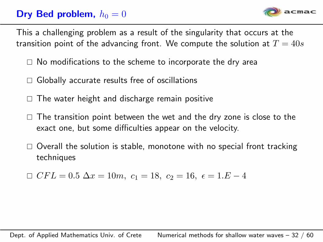
Dry Bed problem, h0 = 0
Dept. of Applied Mathematics Univ. of Crete Numerical methods for shallow water waves – 32 / 60
This a challenging problem as a result of the singularity that occurs at thetransition point of the advancing front. We compute the solution at T = 40s
No modifications to the scheme to incorporate the dry area
Globally accurate results free of oscillations
The water height and discharge remain positive
The transition point between the wet and the dry zone is close to theexact one, but some difficulties appear on the velocity.
Overall the solution is stable, monotone with no special front trackingtechniques
CFL = 0.5 ∆x = 10m, c1 = 18, c2 = 16, ǫ = 1.E − 4

Dry Bed problem, Water Height
Dept. of Applied Mathematics Univ. of Crete Numerical methods for shallow water waves – 33 / 60
0 200 400 600 800 1000 1200 1400 1600 1800 20000
1
2
3
4
5
6
7
8
9
10
x (m)
h (m
)
Dry bed dam-break flow (h), (o)MUSCL with MM limiter.

Dry Bed problem, Discharge
Dept. of Applied Mathematics Univ. of Crete Numerical methods for shallow water waves – 34 / 60
0 200 400 600 800 1000 1200 1400 1600 1800 20000
5
10
15
20
25
30
x (m)
q (m
2 /s)
Dry bed dam-break flow (q), (o)MUSCL with MM limiter.

Dry Bed problem, Velocity
Dept. of Applied Mathematics Univ. of Crete Numerical methods for shallow water waves – 35 / 60
0 200 400 600 800 1000 1200 1400 1600 1800 20000
2
4
6
8
10
12
14
16
18
20
u (m
/s)
x (m)
Dry bed dam-break flow (u), (o)MUSCL with MM limiter.
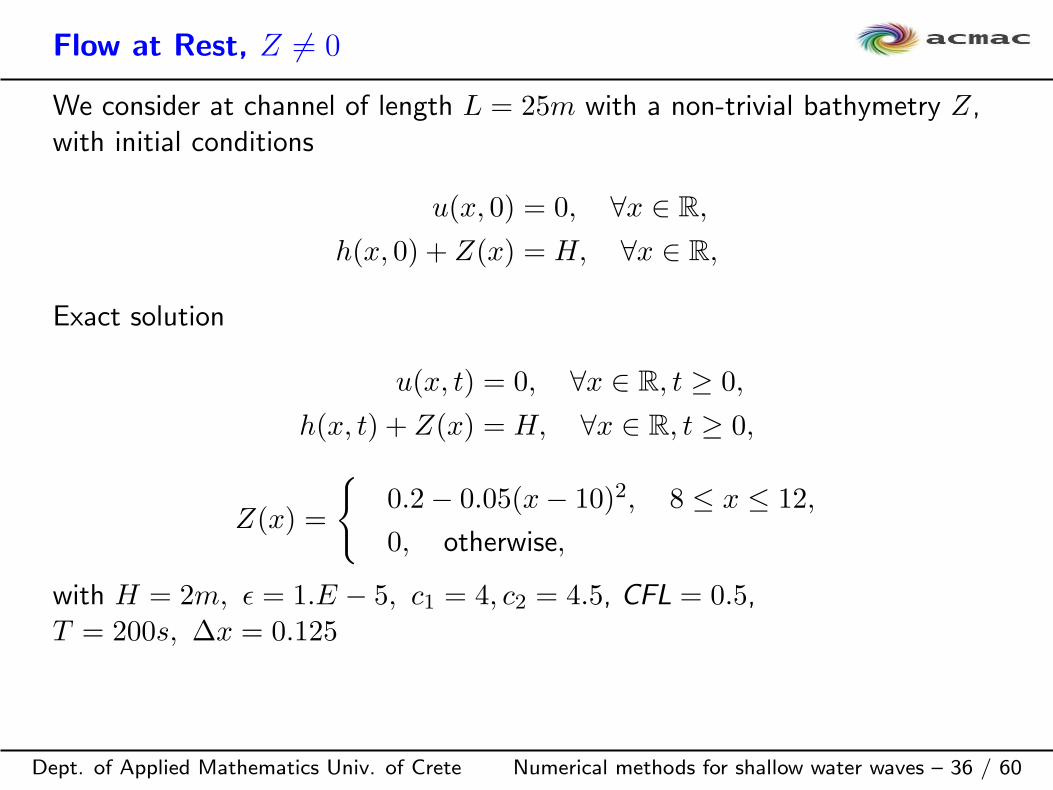
Flow at Rest, Z 6= 0
Dept. of Applied Mathematics Univ. of Crete Numerical methods for shallow water waves – 36 / 60
We consider at channel of length L = 25m with a non-trivial bathymetry Z,with initial conditions
u(x, 0) = 0, ∀x ∈ R,
h(x, 0) + Z(x) = H, ∀x ∈ R,
Exact solution
u(x, t) = 0, ∀x ∈ R, t ≥ 0,
h(x, t) + Z(x) = H, ∀x ∈ R, t ≥ 0,
Z(x) =
0.2− 0.05(x− 10)2, 8 ≤ x ≤ 12,
0, otherwise,
with H = 2m, ǫ = 1.E − 5, c1 = 4, c2 = 4.5, CFL = 0.5,T = 200s, ∆x = 0.125
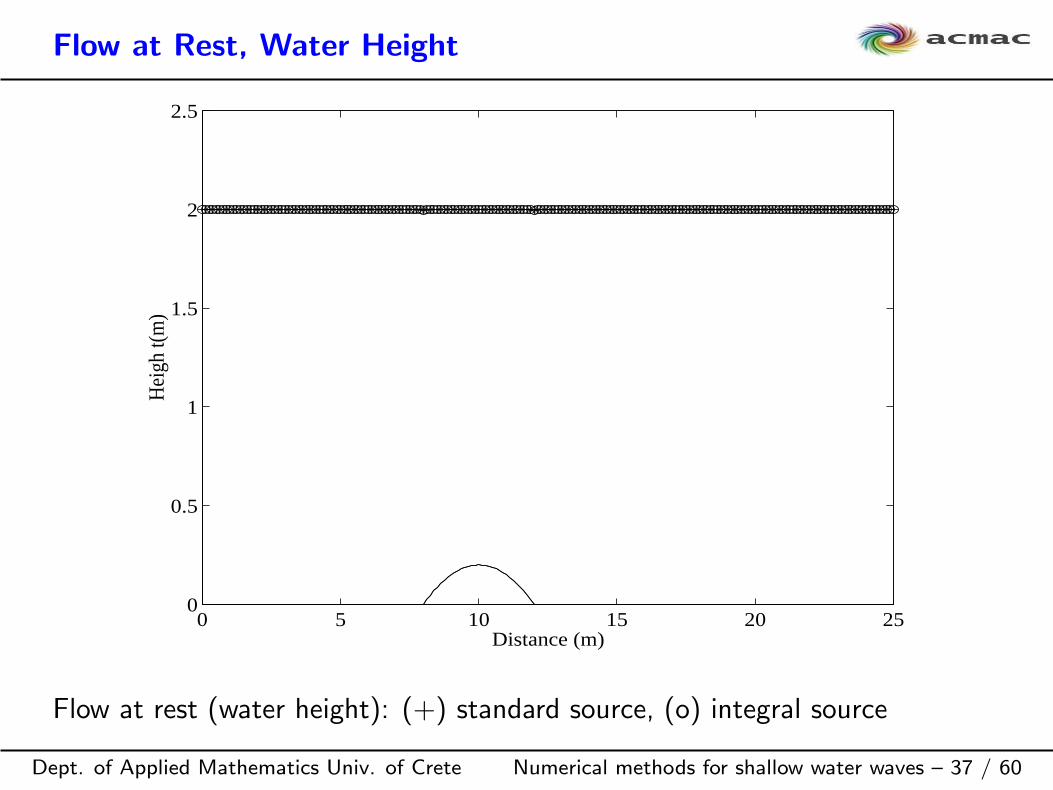
Flow at Rest, Water Height
Dept. of Applied Mathematics Univ. of Crete Numerical methods for shallow water waves – 37 / 60
0 5 10 15 20 250
0.5
1
1.5
2
2.5
Hei
gh t(
m)
Distance (m)
Flow at rest (water height): (+) standard source, (o) integral source
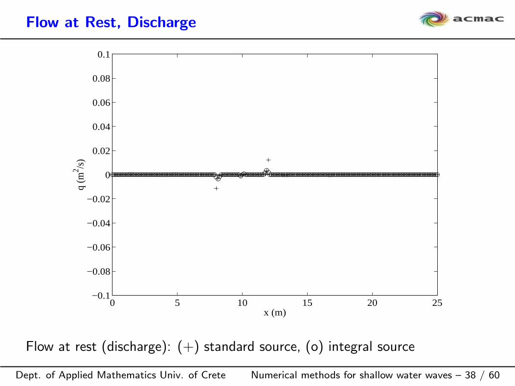
Flow at Rest, Discharge
Dept. of Applied Mathematics Univ. of Crete Numerical methods for shallow water waves – 38 / 60
0 5 10 15 20 25−0.1
−0.08
−0.06
−0.04
−0.02
0
0.02
0.04
0.06
0.08
0.1
x (m)
q (m
2 /s)
Flow at rest (discharge): (+) standard source, (o) integral source

Flow at Rest, Discharge (zoom)
Dept. of Applied Mathematics Univ. of Crete Numerical methods for shallow water waves – 39 / 60
5 10 15 20
−0.01
−0.005
0
0.005
0.01
x (m)
q (m
2 /s)
Flow at rest: Magnified view of the discharge.
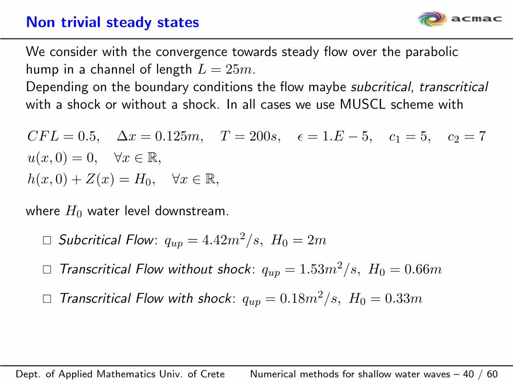
Non trivial steady states
Dept. of Applied Mathematics Univ. of Crete Numerical methods for shallow water waves – 40 / 60
We consider with the convergence towards steady flow over the parabolichump in a channel of length L = 25m.Depending on the boundary conditions the flow maybe subcritical, transcriticalwith a shock or without a shock. In all cases we use MUSCL scheme with
CFL = 0.5, ∆x = 0.125m, T = 200s, ǫ = 1.E − 5, c1 = 5, c2 = 7
u(x, 0) = 0, ∀x ∈ R,
h(x, 0) + Z(x) = H0, ∀x ∈ R,
where H0 water level downstream.
Subcritical Flow : qup = 4.42m2/s, H0 = 2m
Transcritical Flow without shock : qup = 1.53m2/s, H0 = 0.66m
Transcritical Flow with shock : qup = 0.18m2/s, H0 = 0.33m
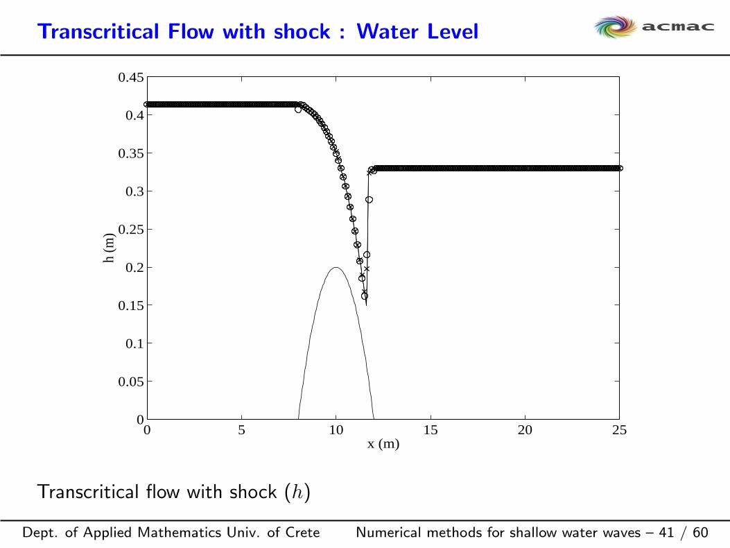
Transcritical Flow with shock : Water Level
Dept. of Applied Mathematics Univ. of Crete Numerical methods for shallow water waves – 41 / 60
0 5 10 15 20 250
0.05
0.1
0.15
0.2
0.25
0.3
0.35
0.4
0.45
h (m
)
x (m)
Transcritical flow with shock (h)
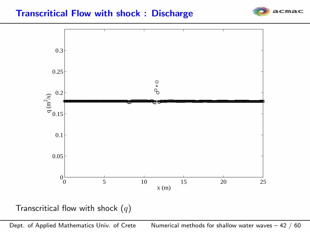
Transcritical Flow with shock : Discharge
Dept. of Applied Mathematics Univ. of Crete Numerical methods for shallow water waves – 42 / 60
0 5 10 15 20 250
0.05
0.1
0.15
0.2
0.25
0.3
x (m)
q (m
2 /s)
Transcritical flow with shock (q)
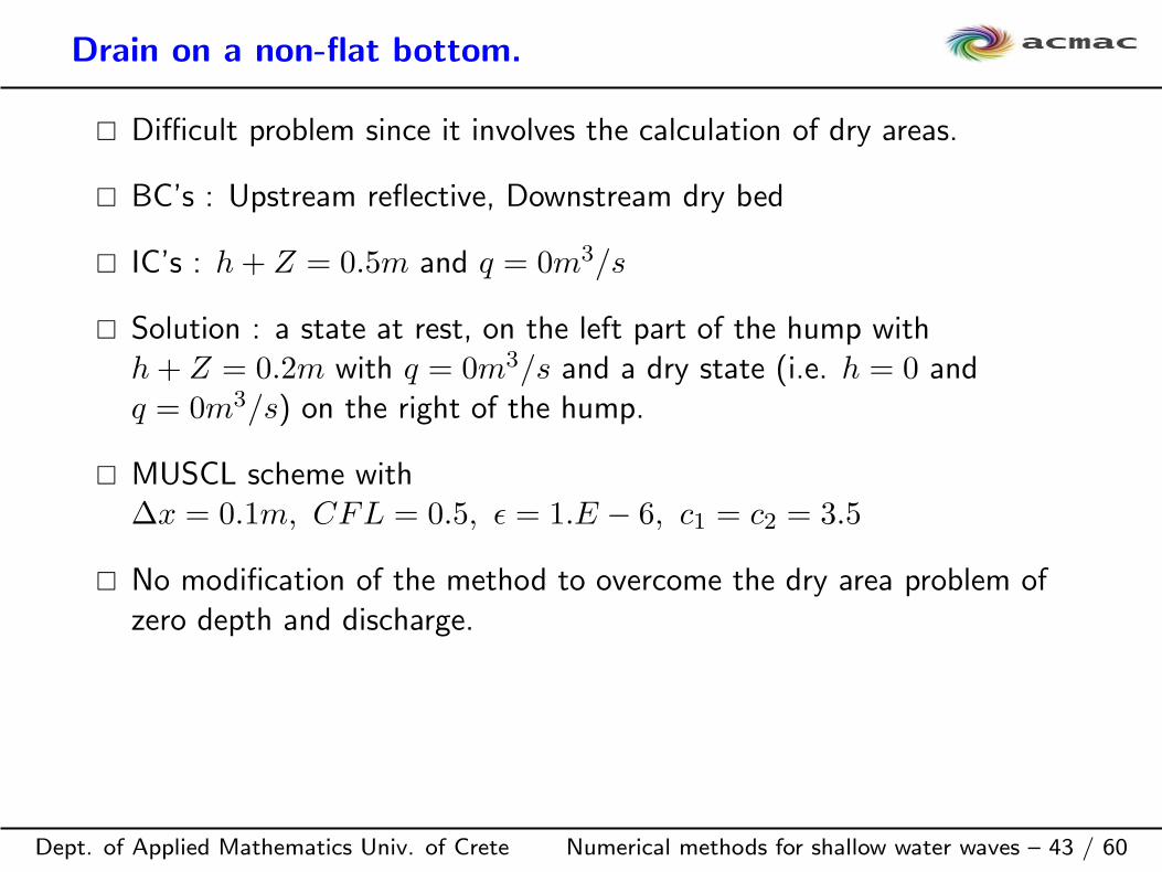
Drain on a non-flat bottom.
Dept. of Applied Mathematics Univ. of Crete Numerical methods for shallow water waves – 43 / 60
Difficult problem since it involves the calculation of dry areas.
BC’s : Upstream reflective, Downstream dry bed
IC’s : h+ Z = 0.5m and q = 0m3/s
Solution : a state at rest, on the left part of the hump withh+ Z = 0.2m with q = 0m3/s and a dry state (i.e. h = 0 andq = 0m3/s) on the right of the hump.
MUSCL scheme with∆x = 0.1m, CFL = 0.5, ǫ = 1.E − 6, c1 = c2 = 3.5
No modification of the method to overcome the dry area problem ofzero depth and discharge.
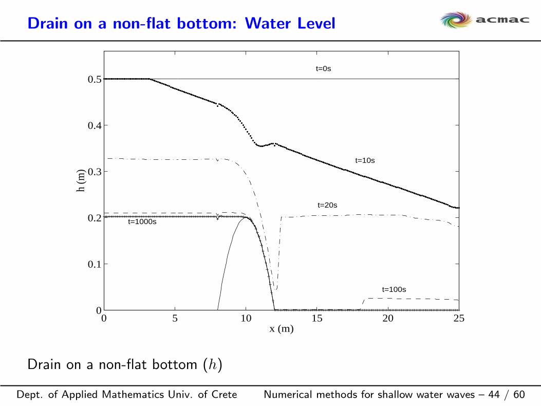
Drain on a non-flat bottom: Water Level
Dept. of Applied Mathematics Univ. of Crete Numerical methods for shallow water waves – 44 / 60
0 5 10 15 20 250
0.1
0.2
0.3
0.4
0.5h
(m)
x (m)
t=0s
t=10s
t=20s
t=100s
t=1000s
Drain on a non-flat bottom (h)
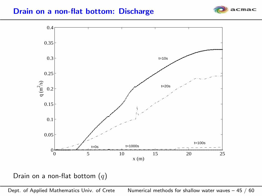
Drain on a non-flat bottom: Discharge
Dept. of Applied Mathematics Univ. of Crete Numerical methods for shallow water waves – 45 / 60
0 5 10 15 20 250
0.05
0.1
0.15
0.2
0.25
0.3
0.35
0.4
x (m)
q (m
2 /s)
t=10s
t=20s
t=100st=1000st=0s
Drain on a non-flat bottom (q)
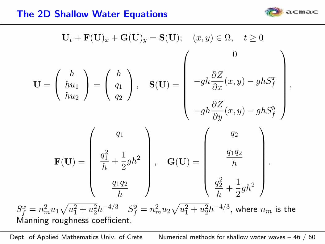
The 2D Shallow Water Equations
Dept. of Applied Mathematics Univ. of Crete Numerical methods for shallow water waves – 46 / 60
Ut + F(U)x +G(U)y = S(U); (x, y) ∈ Ω, t ≥ 0
U =
hhu1hu2
=
hq1q2
, S(U) =
0
−gh∂Z
∂x(x, y)− ghSx
f
−gh∂Z
∂y(x, y)− ghSy
f
,
F(U) =
q1
q21h
+1
2gh2
q1q2h
, G(U) =
q2
q1q2h
q22h
+1
2gh2
.
Sxf = n2
mu1√
u21 + u22h−4/3 Sy
f = n2mu2
√u21 + u22h
−4/3, where nm is theManning roughness coefficient.
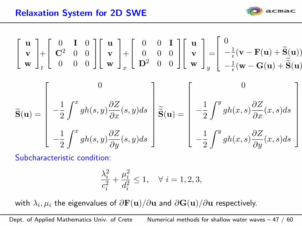
Relaxation System for 2D SWE
Dept. of Applied Mathematics Univ. of Crete Numerical methods for shallow water waves – 47 / 60
u
v
w
t
+
0 I 0C
2 0 00 0 0
u
v
w
x
+
0 0 I
0 0 0D
2 0 0
u
v
w
y
=
0
−1ǫ (v − F(u) + S(u))
−1ǫ (w −G(u) +
˜S(u))
S(u) =
0
−1
2
∫ x
gh(s, y)∂Z
∂x(s, y)ds
−1
2
∫ x
gh(s, y)∂Z
∂y(s, y)ds
˜S(u) =
0
−1
2
∫ y
gh(x, s)∂Z
∂x(x, s)ds
−1
2
∫ y
gh(x, s)∂Z
∂y(x, s)ds
Subcharacteristic condition:
λ2i
c2i+
µ2i
d2i≤ 1, ∀ i = 1, 2, 3,
with λi, µi the eigenvalues of ∂F(u)/∂u and ∂G(u)/∂u respectively.
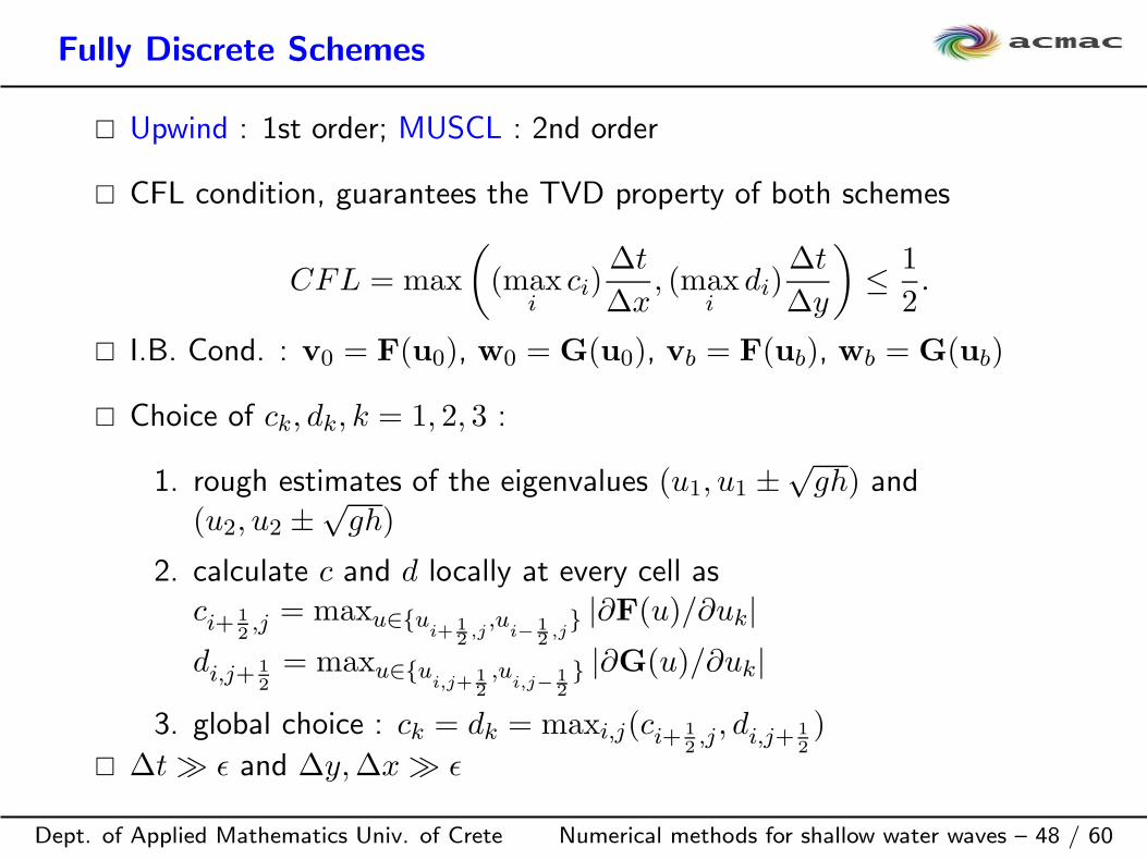
Fully Discrete Schemes
Dept. of Applied Mathematics Univ. of Crete Numerical methods for shallow water waves – 48 / 60
Upwind : 1st order; MUSCL : 2nd order
CFL condition, guarantees the TVD property of both schemes
CFL = max
((max
ici)
∆t
∆x, (max
idi)
∆t
∆y
)≤ 1
2.
I.B. Cond. : v0 = F(u0), w0 = G(u0), vb = F(ub), wb = G(ub)
Choice of ck, dk, k = 1, 2, 3 :
1. rough estimates of the eigenvalues (u1, u1 ±√gh) and
(u2, u2 ±√gh)
2. calculate c and d locally at every cell asci+ 1
2,j = maxu∈u
i+12,j,u
i− 12,j |∂F(u)/∂uk|
di,j+ 1
2
= maxu∈ui,j+1
2
,ui,j− 1
2
|∂G(u)/∂uk|
3. global choice : ck = dk = maxi,j(ci+ 1
2,j , di,j+ 1
2
)
∆t ≫ ǫ and ∆y,∆x ≫ ǫ

Numerical Results for 2D-SWE
Dept. of Applied Mathematics Univ. of Crete Numerical methods for shallow water waves – 49 / 60
No source Z ≡ 0 : Partial Dam Break, Circular Dam Break
Dam break in a channel with topography
2D Partial Dam-Break
Dept. of Applied Mathematics Univ. of Crete Numerical methods for shallow water waves – 50 / 60
The dam, located in the center of a channel breaks instantaneously.
No friction (nm = 0). hu = 10m and hd = 5, 0.1, 0m
Channel : 200m× 200m, 41× 41 square grid.
The breach is 75m in length, 30m from the left bank, 95m from theright.
BC’s : x = 0 and x = 200m transmissive and all other boundaries arereflective.
2nd order MUSCL scheme
ǫ = 10−6 and c1 = 10, c2 = 6, c3 = 11, d1 = 10, d2 = 5, d3 = 11.
T = 7.2s
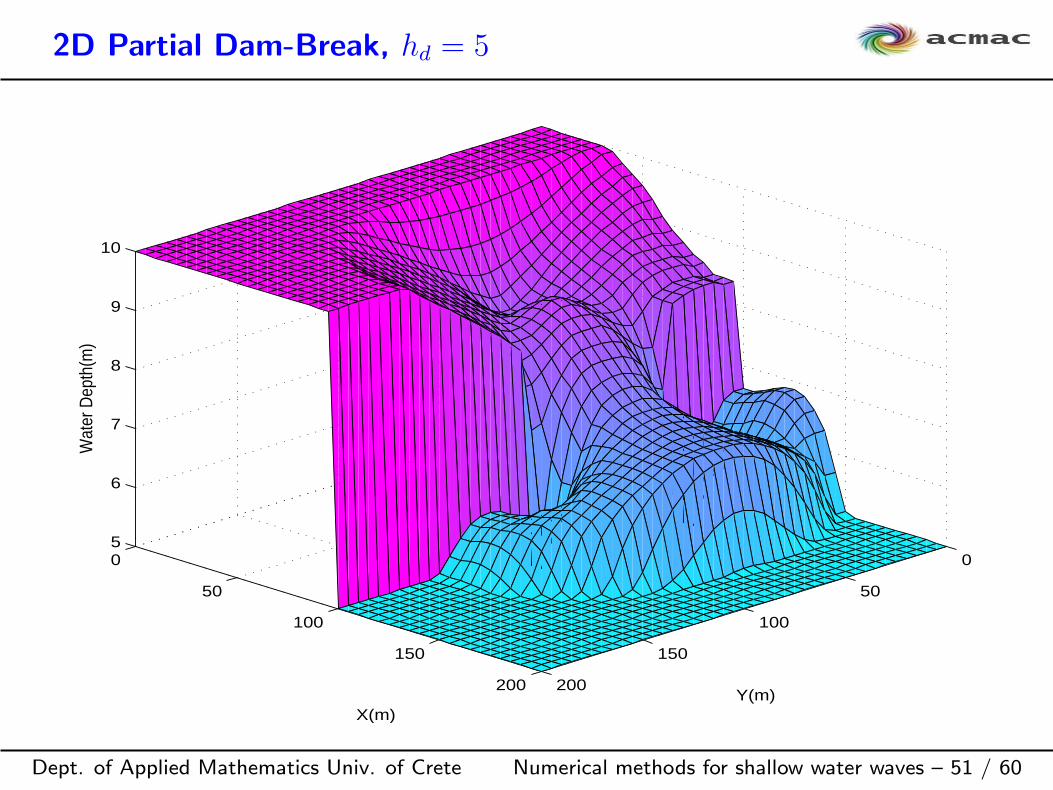
2D Partial Dam-Break, hd = 5
Dept. of Applied Mathematics Univ. of Crete Numerical methods for shallow water waves – 51 / 60
0
50
100
150
200
0
50
100
150
200
5
6
7
8
9
10
Y(m)X(m)
Wat
er D
epth
(m)
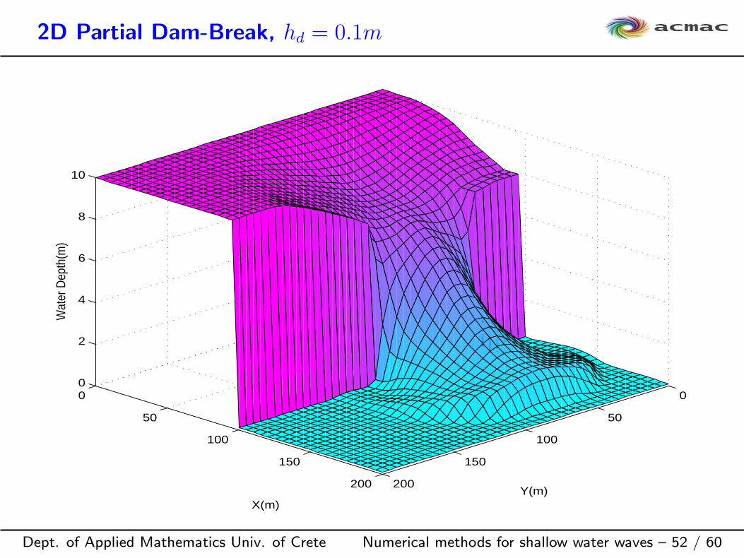
2D Partial Dam-Break, hd = 0.1m
Dept. of Applied Mathematics Univ. of Crete Numerical methods for shallow water waves – 52 / 60
0
50
100
150
200
0
50
100
150
200
0
2
4
6
8
10
Y(m)X(m)
Wat
er D
epth
(m)
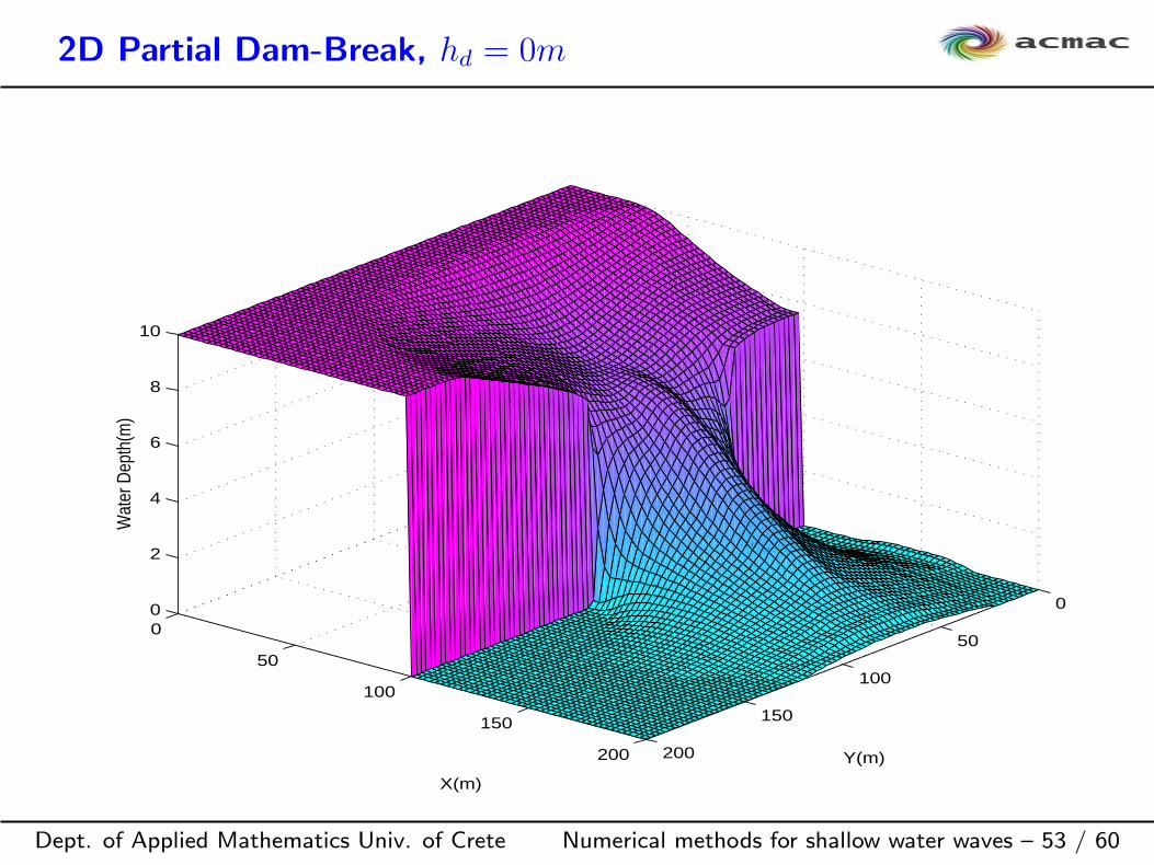
2D Partial Dam-Break, hd = 0m
Dept. of Applied Mathematics Univ. of Crete Numerical methods for shallow water waves – 53 / 60
0
50
100
150
200
0
50
100
150
200
0
2
4
6
8
10
Y(m)
X(m)
Wat
er D
epth
(m)
Circular Dam Break
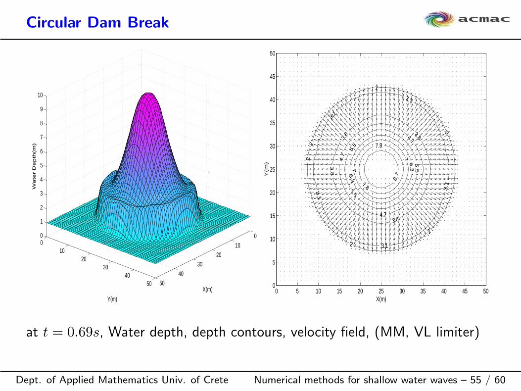
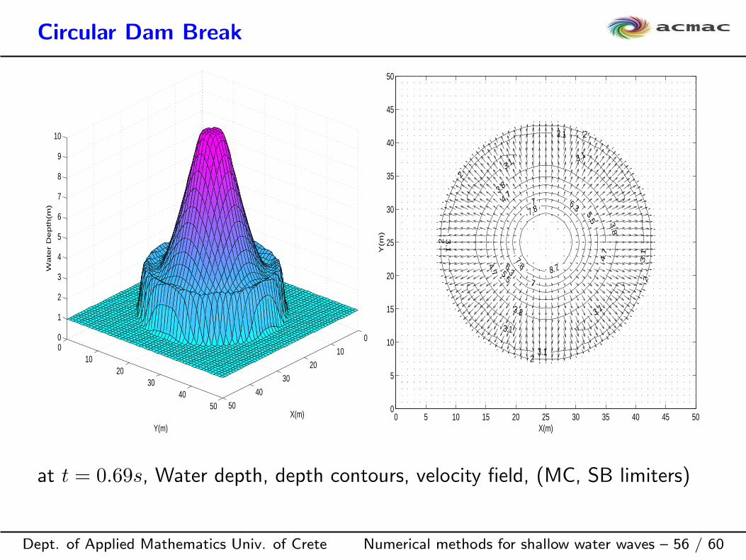
Dept. of Applied Mathematics Univ. of Crete Numerical methods for shallow water waves – 54 / 60
A two dimensional Riemann problem for the 2D SWEs
Two regions of still water separated by a cylindrical wall with radius 11mcentered in a channel. The water depth within the cylinder is 10m and1m outside.
The wall is removed instantaneously, the bore waves will spread andpropagate radially and symmetrically
There is a transition from subcritical to supercritical flow.
2nd order MUSCL scheme
Channel : 50× 50m, 51× 51 square grid
ǫ = 10−6 and c1 = c3 = 12, c2 = 7, d1 = d3 = 12, d2 = 7, T = 0.69s
Circular Dam Break
Dept. of Applied Mathematics Univ. of Crete Numerical methods for shallow water waves – 55 / 60
0
10
20
30
40
50
010
2030
4050
0
1
2
3
4
5
6
7
8
9
10
X(m)
Y(m)
Wate
r D
epth
(m)
0 5 10 15 20 25 30 35 40 45 500
5
10
15
20
25
30
35
40
45
50
X(m)
Y(m
)
2
2
2
2
2
2
3.1
3.1
3.1
3.1
3.1
3.8 3.8
3.8
3.8
4.7
4.7
4.7
5.5
5.5
5.5
6.3
6.3
7
7
7.8
7.8
8.7
at t = 0.69s, Water depth, depth contours, velocity field, (MM, VL limiter)
Circular Dam Break
Dept. of Applied Mathematics Univ. of Crete Numerical methods for shallow water waves – 56 / 60
0
10
20
30
40
50
010
2030
4050
0
1
2
3
4
5
6
7
8
9
10
X(m)
Y(m)
Wate
r D
epth
(m)
0 5 10 15 20 25 30 35 40 45 500
5
10
15
20
25
30
35
40
45
50
X(m)
Y(m
)
2
2
2
2
2
3.1
3.1
3.1
3.1
3.1
3.1
3.1
3.1
3.8
3.8
3.8
4.7
4.7
4.7
5.5
5.5
6.3
6.3
7
7
7.8
7.8
8.7
at t = 0.69s, Water depth, depth contours, velocity field, (MC, SB limiters)

Circular Dam Break, Dry Bed
Dept. of Applied Mathematics Univ. of Crete Numerical methods for shallow water waves – 57 / 60
0
10
20
30
40
50
0
10
20
30
40
50
0
2
4
6
8
10
X(m)Y(m)
Wate
r D
epth
(m)
0 5 10 15 20 25 30 35 40 45 500
5
10
15
20
25
30
35
40
45
50
X(m)
Y(m
)
0.1
0.10.1
0.1
0.1
0.1
0.5
0.50.5
0.5
0.5
0.5
1
1
1
1
1
2
2
2
2
2
3.1
3.1
3.1
3.1
3.8
3.8
3.8
4.7
4.7
4.7
5.5
5.5
5.5
6.3
6.3
7
7
7.8
7.8
8.7
8.7
at t = 0.69s, Water depth, depth contours, velocity field, (VL limiter)

Dam Break in channel with topography
Dept. of Applied Mathematics Univ. of Crete Numerical methods for shallow water waves – 58 / 60
Consider a channel 75m long and 30m wide
A dam is situated at x = 16m with initial water depth h+ Z = 1.875mwhile the rest of the channel is considered dry.
The topography consists of three mounds located in the channelbottom.
Manning coefficient nm = 0.018, ci = di = 5, ǫ = 1.E − 8
Conclusions
Dept. of Applied Mathematics Univ. of Crete Numerical methods for shallow water waves – 59 / 60
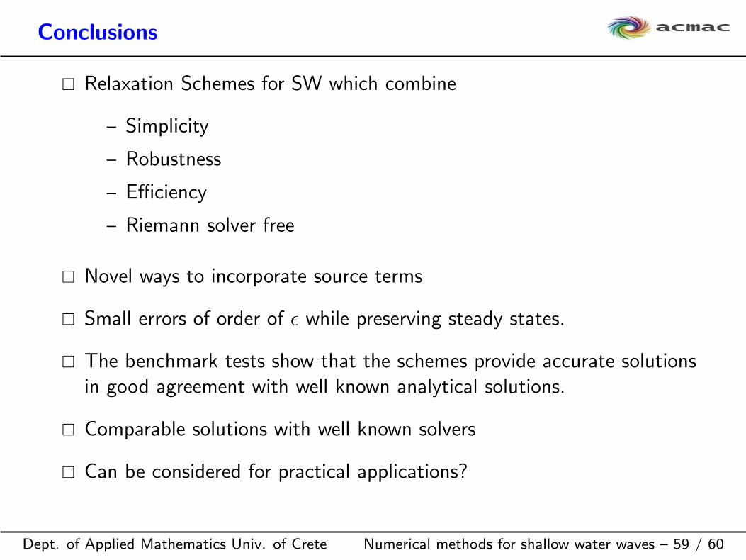
Relaxation Schemes for SW which combine
– Simplicity
– Robustness
– Efficiency
– Riemann solver free
Novel ways to incorporate source terms
Small errors of order of ǫ while preserving steady states.
The benchmark tests show that the schemes provide accurate solutionsin good agreement with well known analytical solutions.
Comparable solutions with well known solvers
Can be considered for practical applications?

References
Dept. of Applied Mathematics Univ. of Crete Numerical methods for shallow water waves – 60 / 60
Jin S, Xin Z. The relaxing schemes of conservations laws in arbitrary
space dimensions. Comm. Pure Appl. Math, 1995
Delis AI, Katsaounis Th., Relaxation schemes for the shallow water
equations, Int. J. Numer. Meth. Fluids, 2003
Delis AI, Katsaounis Th., Numerical solution of the two-dimensional
shallow water equations by the application of relaxation methods, App.Math. Model., 2005
Ch. Arvanitis, Ch. Makridakis, A. Tzavaras, Stability and convergence
of a class of finite element schemes for hyperbolic systems of
conservation laws, SINUM, 2004
Ch. Arvanitis and Th. Katsaounis, Ch. Makridakis, Adaptive finite
element relaxation schemes for hyperbolic systems of conservation laws,M2AN, 2001
Th. Katsaounis, Ch. Makridakis, Relaxation models and finite element
schemes for the shallow water equations, HYP2002, 2003
Related Documents