Numerical Methods I: Numerical Integration/Quadraturestadler/num1/material/num1_quad.pdfNumerical integration Dicult cases for quadrature: I (Unknown) discontinuities in f: adaptive

Numerical Methods I: Numerical

Integration/Quadrature

Georg StadlerCourant Institute, [email protected]

November 30, 2017

1 / 20

Numerical integration

We want to approximate the definite integral

I(f) = Iba(f) =

Z b

af(t) dt

numerically. Properties of the Riemann integral:

I I is linear

I positive, i.e., if f is nonnegative, then I(f) is nonnegative.

I additive w.r. to the interval bounds: Ica = Iba + Icb

2 / 20


Conditioning

Lets study the map

([a, b], f) !Z b

af(t) dt,

where we use the L1-norm for f . The absolute and relativecondition numbers of integration are:

abs

= 1,

rel

=I(|f |)I(f)

.

So, integration is harmless w.r. to the absolute condition number,and problematic w.r. to the relative condition number if I(f) issmall and f changes sign.

3 / 20


We are looking for a map

I :

(C([a, b]) ! Rf 7! I(f)

such that |I(f)� I(f)| is small.

Example: Trapezoidal rule.

General quadrature formula:

I(f) =nX

i=0

�if(ti),

with weights �i and nodal points ti, i = 0, 1, . . . , n.

4 / 20


Newton-Cotes formulas

Replace f by easy-to-integrate approximation f , and set

I(f) := I(f).

Given fixed nodes t0, . . . , tn, use polynomial approximation

f = P (f |t0, . . . , tn) =nX

i=0

f(ti)Lin(t)

Thus:

I(f) = (b� a)nX

i=0

�inf(ti),

where �in = 1b�a

R ba Lin(t) dt

5 / 20



Theorem: For (n+ 1) pairwise distinct points, there exists exactlyone quadrature formula that is exact for all p 2 P n.

Uniformly spaced points:

�in =1

b� a

Z b

a

Y

i 6=j

t� titi � tj

dt =1

n

Z n

0

Y

i 6=j

s� j

i� jds

These weights are independent of a and b.

9.2. Newton-Cotes Formulas 275

the constructed quadrature formulas are called Newton-Cotes formulas. The term for the corresponding Newton-Cotes weights Ain simplifies via the substitution s := (t - a)/h:

1 lb n t - tj 1 in n S - j Ain = -- II-- dt= - II-- ds.

b - a a j=O ti - tj n 0 j=O i - j j#i j#i

The weights Ain, which are independent of the interval boundaries, only have to be computed once, respectively, given once. In Table 9.1, we have listed them up to order n = 4. The weights, and therefore also the quadra-ture formulas, are always positive for the orders n = 1, ... , 7. Higher orders are less attractive, since starting with n = 8, negative weights may occur. In this case, the Lebesgue constant is the characteristic quantity (9.3), up to the normalization factor (b - a)-I. Note that we have already encoun-tered the Lebesgue constant in Section 7.1 as the condition number of the polynomial interpolation.

Table 9.1. Newton-Cotes weights Ain for n = 1, ... ,4.

n AOn , ... , Ann Error Name

1 1 1 1" (,) Trapezoidal rule "2 "2

2 1 4 1 Simpson's rule, Kepler's barrel rule (; (; (;

3 1 3 3 1 3:05 f(4)(,) Newton's 3/8-rule 8 8 8 8

4 7 32 12 32 7 f(6)(,) Milne's rule 90 90 90 90 90

In Table 9.1, we have already assigned the respective approximation er-rors to the Newton-Cotes formulas (for sufficiently smooth integrands), expressed as a power of the step size h and a derivative at an intermediate position, E [a, b]. Observe that for the even orders n = 2,4, the power of h and the degree of the derivative always jump by 2. In the following we shall verify these estimates for the first two formulas, by which one can already see the principle for odd n (see Exercise 9.3).

Before starting, we recall a not so obvious variant of the mean value theo-rem, which we shall encounter repeatedly in the proof of the approximation statements.

Lemma 9.5 Let g, h E C[a, b] be continuous functions on [a, b], where g has only one sign, i.e., either g(t) 2: 0 or g(t) ::; 0 for all t E [a, b]. Then

lb h(t)g(t) dt = h(,) lb g(t) dt

for some, E [a, b].

Weights are positive up to order 7, then some become negative.6 / 20



Proof of error terms is based on

I a variant of the mean value theorem for integrals

I the Newton remainder form from interpolation, e.g., for linearinterpolation

f(t)� P (t) = [t, a, b]f · (t� a)(t� b) =f 00(⌧)

2(t� a)(t� b).

For piece-wise polynomial approximations (e.g., the trapezoidalrule), analogous estimates as shown in the table hold.

7 / 20


Gauss-Christo↵el quadrature

Now, let’s allow the nodes t0, . . . , tn to vary. The best we canhope for is exact interpolation up to polynomials of degree 2n+ 1(based on a non-rigorous counting argument).

Also, for generalization, we consider quadrature of weightedintegrals, with a positive weight function !(t):

I(f) =

Z b

a!(t)f(t) dt

with weight funcations !(t) = 1,!(t) = 1/p1� t2, . . ..

8 / 20



Theorem: If I is exact for polynomials p 2 P 2n+1 (for !-weightedintegration), then

Pj+1(t) = (t� ⌧0j) · . . . · (t� ⌧jj) 2 P n+1

are orthogonal with respect to the scalar product induced by !(t).

9 / 20



Thus:

I one must choose the roots of the orthogonal polynomials(which are single roots)

I the weights are uniquely determined and yield exactintegration for polynomials up to degree n. . . but:

Theorem: Let ⌧0n, . . . , ⌧nn be the roots of the (n+ 1)st orthogonalpolynomial for the weight !. Then any quadrature formula I isexact for polynomials up to order n if and only if it is exact up toorder 2n+ 1.

10 / 20



11 / 20



9.3. Gauss-Christoffel Quadrature 285

Table 9.3. Commonly occurring classes of orthogonal polynomials.

w(t) Interval I = [a, b] Orthogonal polynomials

1 [-1,1] Chebyshev polynomials Tn v'1-t2

e- t [0,00] Laguerre polynomials Ln

e- t2 [-00,00] Hermite polynomials Hn

1 [-1,1] Legendre polynomials Pn

(w == 1) is only used in special applications. For general integrands, the trapezoidal sum extrapolation, about which we shall learn in the next sec-tion, is superior. However, the weight function of the Gauss-Chebyshev quadrature is weakly singular at t = ±1, so that the trapezoidal rule is not applicable. Of particular interest are the Gauss-Hermite and the Gauss-Laguerre quadrature, which allow the approximation of integrals over infinite intervals (and even solve exactly for polynomials P E P 2n+1)'

Let us finally note an essential property of the Gauss quadrature for weight functions w t 1: The quality of the approximation can only be improved by increasing the order. A partitioning into subintervals, however, is only possible for the Gauss-Legendre quadrature (respectively, the Gauss-Lobatto quadrature; compare Exercise 9.11).

9.3.2 Computation of Nodes and Weights

For the effective computation of the weights Ain, we need another represen-tation. For this purpose, let {Fd be a family of orthonormal polynomials Fk E Pk, i.e.,

(Fi' Fj ) = bij .

These satisfy the Christoffel-Darboux formula (see, e.g., [82] or [64]).

Lemma 9.14 Suppose that kn are the leading coefficients of the or-thonormal polynomials Fn(t) = kntn + O(tn- 1 ). Then, for all 8, t E

R,

(Fn+l (t)Fn(s) - Fn(t)Fn+l (8)) = t Fj(t)Fj(s) . kn+l t - s .

J=O

The following formula for the weights Ain can be derived from this formula.

Lemma 9.15 The weights Ain satisfy

(9.5)

Corresponding quadrature rules are usually prefixed with “Gauss-”,i.e., “Gauss-Legendre quadrature”, or “Gauss-Chebyshevquadrature”.

12 / 20


Gauss-Legendre points/weights for interval [�1, 1]

13 / 20


Gauss points in 2D

Tensor-product Gauss points. Weights are products of 1D-weights.

14 / 20


I Accuracy in Gauss-(Chebyshev, Laguerre, Hermite,Legendre,. . . ) can only be improved by increasing number ofpoints

I Of particular interest are quadrature points for infiniteintervals (Laguerre, Hermite)

I Interval partitioning superior, but only possible for ! ⌘ 1(Gauss-Legendre or Gauss-Lobatto)

0

3

1

4

2

2D-Gauss-Lobatto integration points (also used as interpolation points).

15 / 20

Integration on [0,1] (Laguerre)

How to approximate Z 1

0g(t) dt,

where g decays rapidly enough such that the integral is finite?Laguerre integration assumes integration weighted with e�t. . .

16 / 20


Interval partitioning

Split interval [a, b] into subintervals of size h = (b� a)/n. Basictrapezoidal sum:

T (h) = Tn = h

1

2(f(a)� f(b)) +

n�1X

i=1

f(a+ ih)

!

We can now think of what happens as h ! 0 (i.e., moresubintervals).

Theorem: For f 2 C2m+1 holds:

T (h)�Z b

af(t) dt = ⌧2h

2 + ⌧4h4 + . . .+R2m+2(h)h

2m+2,

which coe�cients ⌧i that depend on the derivatives of f at a andb, and on the Bernoulli numbers B2k and R2m+2(h) is a remainderterm that involves f (2m).

17 / 20


Interval partitioning

Extrapolation:limh!0

T (h) := limn!1

Tn = I(f)

Extrapolation uses h1, . . . , hn to estimate the limit.

I One can estimate the order gained by extrapolationtheoretically (Thm. 9.22 in Deuflhard/Hohmann).

I Existence of an asymptotic expansion with a certain order hp

(p � 1) can be used to improve the extrapolation.

I Extrapolation ideas with Trapezoidal rule leads to Rombergquadrature.

18 / 20


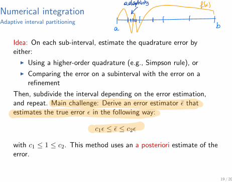
Adaptive interval partitioning

Idea: On each sub-interval, estimate the quadrature error byeither:

I Using a higher-order quadrature (e.g., Simpson rule), or

I Comparing the error on a subinterval with the error on arefinement

Then, subdivide the interval depending on the error estimation,and repeat. Main challenge: Derive an error estimator ✏ thatestimates the true error ✏ in the following way:

c1✏ ✏ c2✏

with c1 1 c2. This method uses an a posteriori estimate of theerror.

19 / 20


Di�cult cases for quadrature:

I (Unknown) discontinuities in f : adaptive quadrature continuesto refine, which can be used to localize discontinuities

I Highly oscillating integrals

I (Weakly) singular integrals (as required, e.g., in integralmethods (the fast multipole method)

20 / 20

Numerical Methods I: Numerical Integration/Quadraturestadler/num1/material/num1_quad.pdfNumerical integration Dicult cases for quadrature: I (Unknown) discontinuities in f: adaptive

Documents