Numerical Methods: Finite Difference Approach

Numerical Methods: Finite Difference ApproachDr. Ameeya Kumar Nayak

Department of MathematicsIndian Institute of Technology, Roorkee

Lecture – 02Numerical solution of ODE

Welcome to the lecture series on numerical methods, finite difference approach. In the

last lecture, I have discussed about like finite difference approximations, so based on

Taylor series approximation and Picard’s method.

(Refer Slide Time: 00:32)

So, in this lecture, I will just go for like numerical methods based on this Euler’s method,

and Modified Euler’s method. And then we will just go for a Runge-Kutta method.

So, in the last lecture, I have just discussed that whenever we will have like a higher

order differential equations, with the initial conditions, then we can just reduce all the

higher order differential equations into the set of or linear differential equations. So, if it

is like order 1 equations are existing, then we can just use either this a Picard’s method or

the Taylor series expansion. Then we are just proceeding in a form that once we are just

really have like Picard’s method, then we will just try to improve that method; that is, in

the form of like Euler’s method.

And once it is a Euler’s method we have then we will just go for some higher order

methods, that is in the order of like, order 2 that is as Euler’s method here. Then like a to

improve this Euler’s method again we will just go for this modified Euler’s method.

Then the improved form of this modified Euler’s method is nothing but they Runge-

Kutta method here.


So, if will just go for this Euler’s method here, so the same problem, we can just consider

that is like, if you will just see here dy by dx, dy by dx that is nothing but f of x y. And

your initial condition that is given as y of x 0 equals to y 0 here. So, if the initial

condition is a written in this form here, then first we will just go for a graphical approach

that, if a curve is given so at certain points we will have this differential representation;

this means that, this is just a satisfied or this differential equation is given at the point x 0

and y 0.


So, if this differential equation is a provided at certain point, then at that point it can just

form a slope with the tangent line, and if the tangent line is forming at that point, then

based on that we can just derive this Euler’s formula. So, in order to achieve this formula

if you will just go for a true solution here true solution means we can just distinguish

these solutions in 2 forms. One it is called a true solution which is based on these

numerical methods, another one it is called analytical solution or the exact solution;

which can be obtained by using any of this like real analysis methods. This is where

specifically called numerical analysis, that is called a real analysis methods.

So, to often this true solution at y equals to f of x since dy by dx is provided at the point

x 0 and y 0 there, if you will just set up these coordinates here that is in the form of like x

0; x 0 means at this point we can just put this point as x 0 here. And corresponding to this

we will have a y 0 point here. And at that point only we have this dy by dx slope can be

found with a tangent. So, especially if we will just consider y equals to f of x is the true

solution. And the exact value of y at x equals 2 x 1, suppose on that car if you will just

consider as Q here, that is nothing but y 1 value here.

So, corresponding to y 1, we will have an improvement in a x 1 also. That is nothing but

we can just consider as x 0 plus h here that is nothing but x 1. So, h means that, is

nothing but the space length from here to here there. So, x 0 to x 1 the space length is h

we have consider, and if you will just consider this Euler’s method to approximate this

value at y at x equals 2 x 1 here, we can just assume dy by dx is provided as f of x 0 and

y 0; which is the slope of the tangent PR, if you will just see, this is the tangent forming

at the point x 0 and y 0, which is just intercepting this line Q N; that is nothing but the

next functional value with the corresponding x 1 value there over.

So, if you will just take this f of x 0 and y 0 that is nothing but 10 theta, since it deforms

the slope here. So, 10 theta is nothing but we can just say that this is p this is a b here.

So, 10 theta is nothing but p by b here, and if you will just define this RS here that is

nothing but, we can just write h 10 theta here, 10 theta especially we are just considering

slope means 10 theta there over.

So, that is why we are just writing f of x 0 and y 0 this equals to 10 theta here. So, then

RS equals to h 10 theta, then we can just so define the total distance from here to here

RN, that is nothing but SN plus h 10 theta. So, SN means we can just consider SN is

nothing but y 0 distance from here.


So, we can just write this one as like the next immediate value that is a RN, if you will

just see here RN can be added with like a QR here. So, then we can just find the total

distance that is nothing but QN here.

So, if you will just write RN here, RN can be written as like SN plus h 10 theta here. So,

h 10 theta means, we can just say that y 1 can be written in the form of y 0 plus h f of x 0

and y 0 here and the error associated with this value that is given by QR, which is given

by R equals to h square by 2 factorial f dash of zeta here.

Since, if you look at this picture here, the error means we can just say that the

improvement that is just taken from y 0 to y 1 there over. So, for that if you will just

consider this difference see here, that is nothing but h square by 2 factorial f does zeta

here.

So, the Euler’s formula is can be written as like a yn plus 1 this equals 2 yn plus h f of xn

and yn here, since the beginning if we are just approximating this formula is in the form

of like y 1 equals to y 0 plus h f of x 0 y 0, that is nothing but the y 1 improvement if you

will just consider from this line here that is nothing, but this error term it is just in a large

sense we can just consider, and afterwards if you will just consider this error term again

one more slope we have to consider, which can reduce the error term there over that is

why, if we are just considering this a higher order term see here that is as one in the fast

sense it is written in the form of y 0 plus h f of x 0 and y 0 here, and the second one we

can just write this one as y 2 this is nothing but y 1 plus h f of x 1 y 1 here.

Similarly, if you will just proceed, then in the inert form we can just write this one as yn

plus 1 this is nothing but yn plus h f of xn yn here, with the error term R equals to h

square by 2 factorial f dash of zeta n y, since this error term always represented in the

first order differential equation from here, where zeta m should be lies between xn to xn

plus 1 since whenever the slope is increasing from point to point this error is getting

reduced and this error lies between this immediate below point to the next approximated

value. So, that is why in the beginning I have just told that this a error for this Euler’s

formula is of order of h square or the second order approximation we are just getting for

the error terms.


And if you will just go for a practical example here, that is based on Euler’s method here

suppose the question is given like using Euler’s method, compute y1 and y 2 taking h

equals to 0.1 from the following differential equation, that is as dy by dx equals to 1 plus

xy square y 0 equals to 1 here also compute the error term there. So, if you will just go

for this equation here, especially we can just write this equation as dy by dx that is

nothing but your f of xy here, which is represented in the form of 1 plus xy square and y

0 is a provided as 1 here. So, that is why we can just write y dash as f of xy that is

nothing but 1 plus xy square, and y doubled dash we can just express this is nothing but f

dash of x y this is nothing, but we can just write y square plus 2 xy 1 plus xy square here.


Since, say already we have explained that one f dash of x y is nothing but, we can just

write it as fx plus fy into f here. So, that is why I have just written in this form here. So,

then especially for x equals to 0.1 here, we can just write y 1 equals to y 0 plus h f of x 0

y 0 here. So, if you will just write in this form since, every value it is known to us y 0

equals to 1 here x 0 equals to 0 here.

So, if I will just use this values, then I can just write this one as y 1 this can be written as

like 1 plus h is nothing but it is just as specified as a like 0.1. So, that is why 0.1 into

your f of x I value that is nothing but I can just write as like 1 plus x 0 y 0 square here.

So, if I will just do this one like the final form of this one 1 plus 0.1 into 1 here, that is

nothing but 1.1. So, in the error term if you will just go for this computation. So, epsilon

one this can be written as like half h square like y double dash of zeta here, since f dash

zeta it is just written in the formulation so that is why it is written as half h square y

double dash of zeta this can be written as half of like h square f dash of zeta y where,

zeta should be lies between like 0 to 0.1 here, and especially I can just write 0.5 into 0.01

into 1.45662 here.

Since, f dash of zeta y if you will just see this is nothing but 1.45662 here, at x equals to

0. So, that is why this final value it will just achieve as a 0.0078. So, that is why this final

solution we are just obtaining that is the order of h square if you will just see 0.0078, it is

just a represents that value corresponding to h equals to 0.1 here.


So, then for x equals to 0.2 if you will just use this formula recursively, then again, we

can just write this formula as y 2 equals to y 1 plus h f of x 1 y 1 here. So, if you will just

put the value here that is y 2 equals to y 1 plus h f of x 1 y 1 here. So, that is why y 1 is

just if you will just see the value here that is just a given as 1.1 here over.

So, that is why 1.1 plus h that is nothing but 0.1 here into your value so that is as a

functional value, that as like a 1 plus xy square here, 1 plus xy square means so we can

just write as x plus y square means 1.1 it is just giving. So, final value we can just write

that as 1.2121 here.

So, maximum truncation error or error propagated from fast f plus the local truncation

error that, is we can just write as epsilon 2 equals to epsilon 1 into 1 plus h fy of x 1 y 1

here since this error this is associated with the second approximation here. So, that is

why we can just consider plus half of hs square f dash of zeta y plus the local error that it

has been associated or already it is associated there over this is the error term here.

So, in the complete form if you will just write this total error here, this error can be

written as epsilon 1 into 1 plus this h is there so fy of x 1 y 1 that is nothing but 2 h x 1 y

1 plus half h square into y square plus 2 xy into 1 plus x y square here. So, if you will

just put all these values h equals to 0.1 and x 1 is it can be written as in the form of a 0.1

also there and y 1 it is just at the computed value, that is as a 1.1 if you will just see this y

1 value is coming as 1.1 here. So, that is why it can be written as like 0.00728 into 1.022

plus 0.005 into 1.4692 plus 0.6272 here, and the final answer just it is just giving you

0.0179.

If you will just see this previous staff error. So, this error is just a given as a 0.00728 and

in the next step this error is reduced to like 0.0179 here. So, whenever we will just go for

like higher steps then the error will be minimized afterwards.


So, then we will just go for like modified or improved Euler’s method. So, in the Euler’s

method especially we are just using only this a positive values that as like y 1 equals to y

0 plus h f of x 0 y 0 there, and in the modified Euler’s form we can just take the average

of like previous step calculation into the plus the next step calculation, and it can be since

we are just taking the average values of these two we can just a modified form we can

just write this formula is y 1 equals to y 0 plus h by 2 into f of x 0 y 0 plus f of x 1 and y

1 there.

Since, two unknowns are associated in this formula here, if you will just see 2 formulas

are associated here. So, that is why we can just consider this y 1 star it can be computed

from the earlier step by using only Euler’s method, there so Euler’s method especially it

is written as y 1 equals to y 0 plus h f of x 0 y 0. So, that is why from this we can just

calculate this y 1 star at the beginning of the problem, then successively we can just pour

these values in this formulation here, and if you will just see in a fundamental way also

this can improve the nature of this approximation compared to the earlier one.

So, that is why I have just written this statement the Euler’s method is given by like yn

plus 1 equals yn plus h f of x n yn here, having the error of order of h square here second

order and the modified Euler’s method is an improvement over the earlier method giving

the error in the order of h q here, and in this method especially y 1 can be obtained by

using the earlier Euler’s method and it can be improved by taking the average value of

the gradients of f of x 0 y 0 and f of x 1 y 1 star since, y 1 is unknown to us that is why

we are just using this earlier Euler’s method to get the value of y 1 in a improved form or

in a modified form.

So, then if you will just take k is h of f of x 0 y 0, then we can just write this one or in the

modified form y 1 can be written as y 1 equals to y 0 plus h by 2 f of x 0 y 0 plus f of x 0

plus h that is nothing but x 1 here and then y 1 star which can be written as like y 0 plus

h f of x 0 y 0 since already we have defined here that is as a k 1 here, k 1 is nothing but h

f of x 0 y 0 which can be written as y 0 plus k 1 here.


So, for the further improvement if you will just go for the error in the modified Euler’s

method to for this error, if you will just expand this Taylor series as y 1 equals to y 0 plus

h by 2 f of x 0 y 0 plus h by 2 if you will just take the next term that is as f of x 0 y 0 plus

h del f by del x plus k del f by del y plus half h square del square f by del x square plus 2

hk del square f by del x del y plus k square del square f by del y square plus all other

terms especially, we are just taking this one as in the form y one equals to y 0 plus h by 2

f of x 0 y 0 plus h by 2 f of x one y 1 there itself.

So, that is why we are just considering since x 1 can be written in the form of like x 0

plus h, and y 1 can be written in the form of y 0 plus hf there. So, that is why it can be

expanded in Taylor series form and in the if you will just expand all the terms then this is

the combined form of this all the terms here, if you will just use like k equals to suppose

h f of x 0 y 0 here, then we can just get the series as y 1 equals to y 0 plus h f y 2 plus h

by 2 if you will just see then f plus h into del f by del x since, k is replaced by here h f of

x 0 y 0 so h can be taken common. So, f can be multiplied with this storm. So, it can be

written in a compact form here.

So, similarly if we in this term also if you will just replace k by h f of x naught y naught.

So, it can be represented as a 2 h f del square f y del x del y plus h is f square del square f

y del y square here, and in the final form if you will just see. So, this can be written as y

0 plus hf plus, if we will just take common from all other terms that is if you will just see

here h del f by del x here plus hf del f by del y here.

So, if you will just write in a compact form that is if you will just take like h f by 2 and

add it off then we can just write this one as or if you will just subtract this h f y 2 from

both these terms this can be represented as hf plus h square by 2 del f by del x plus f del f

by del y so remaining terms have there. So, only we are just adding h by h f by 2 term

here subtracting from this one, or you can just consider this addition of these 2 terms can

be represented in this form here.


So now if you we want to find the exact solution that has y of x 0 plus h that is nothing

but y of x 1. So, if you will just take the Taylor series expansion. So, directly we can just

obtain this Taylor series expansion as y of x 0 plus h. So, which can be written as y 0

plus h y 0 dash plus h square by 2 y 0 double dash plus h cube by 3 factorial y 0 triple

dash and if you will just subtract like from the earlier formulation here y1 is there and

this is y of x 1 is here if you will just take the difference, then we can just find that this

term is 0 this term is 0 this term is 0 here and we can just obtain a subtracted term that is

in the form of minus h cube by 2 l del square f by del x square plus 2 f del square f by del

x del y plus f square del square f by del y square plus 2 del f by del y and y double dash

here, that is nothing but order of h cube.

So, we are just finding this improved form of this like Euler’s method, if you are just

going for like higher approximations. So, in the earlier method we have just obtained this

error is of order of h square here we are just obtaining this error is of order of h cube

here.


If you will just go for a practical example that is specifically if it is written in the form of

like dy by dx equals to x minus y and y 0 equals to 1 here for x equals to starting point is

like x naught equals to 0.2 and it is incremented by 0.2 and last point is 0.4 here. So, that

is why it is just written as like x naught equals to 0.2 incremented by 0.2 here.

So, that is why we can just consider like x 1 this can be written as 0.2 plus 0.2 that is

nothing but 0.4 here. So, initial value of x 0 is 0.2 and x 1 is like 0.4.

So, two step calculation we have to move here. So, for x equals to 0.2 here, if we I will

just write the increment here increment means, I am just writing h equals to 0 point here.

So, if you will just consider here that is as y of 0 is 1 here, especially we can just write x

0 equals to 0 and y 0 equals to 1, then the first improvements if you will just consider

here that has like y 0 as 1 then we have to find y 1 here and x 0 is a given 0 here then x 1

is given as x 0 plus h that is nothing but 0.2 here.


So, based on this we will just find first y 1 star here. So, for y 1 star if you will just

consider like y 0 plus h f of x 0 y 0 here, then y 0 is given as a one especially, I am just

putting here then h is given as a 0.2 here then the formula that is as x 0 minus y 0 here.

So, x 0 is a 0 here minus y 0 is 1 here. So, if you I will just take the total sum of the term

here so that is just giving you a 0.8 here.

So, the immediate improvement if we want to find since y 1 star, we can just write this is

the calculation from Euler’s method only original Euler’s method and then if we want to

find a modified form or a improve form of this Euler’s method then y 1 can be written as

y 0 plus h by 2 f of x 0 y 0 plus f of x 1 y 1 star here. So, y 0 is given as a 1 here then h is

0.2 by 2 then f of x 0 y 0 it is just obtained as like, if you will just see here that is x 0

minus y 0 here that is a minus 1 then plus we can just write h by 2 0.2 by 2 here. So, like

f of x 1 y 1 star here. So, y 1 star it is just computed as 0.8 here, see if you if I will just

put x 1 as 0.2 minus 0.8 here.


So, final answer it is just coming as a 0.84 here, for x equals to 0.4 that is a we can just

consider x 1 as a 0.2 here then x 2 equals to 0.2 plus 0.2 that is nothing but 0.4 here. So,

at y at 0.4 especially, we can just say this one this can be obtained if you will just first

compute y 2-star y 2 star can be written as y 1 plus h f of x 1 y 1 here, that is y 1 can be

written as 0.84 plus 0.2 into 0.2 minus 0.84, and the value is coming as 0.712 and

specifically based on this y 2-star value we can just compute y 2 here.

So, y 2 can be written as y 1 plus h by 2 f of x 1 y 1 plus f of x 2 y 2 star here. So, if you

will put y 1 value that is nothing but 0.84 here. So, h is 0.2 by 2 here then f of x 1 y 1 that

is nothing but minus 0.64 plus 0.4 minus 0.712 here, and the final value it is just

obtaining as 0.7448 here.

So, analytic solution it can be often if you will just take the direct integration of this

differential equation and the value can be obtained as like x minus 1 plus 2 e to the

power minus x here, and if we want to compute the value at the 0.2 so as specifically if

you will just put here like x equals to 0.2, then the value is given as 0.8375 here and for

0.4 the value is given as 0.7406 and if you will take this difference between these 2

values, then we can just find the error in that method then we will just go for like a

Runge-Kutta method here.


Runge-Kutta method is nothing but the improvement of like modified alerts method if

you will just see here we are just considering different terms as in the form of like k 1 as

a function of like h f of x 0 y 0 k 2 as f of x 0 plus h by 2 y 0 plus k 1 by 2 this is nothing

but the improvement of like k 1 term in this term here then again we will just take an

improvement of k 2 term in the next term here, then again we will just consider a next

improvement of the previous term in the next term there itself.

If you will just take the combination of all the terms here, then we can just obtain the

final improvement of this term here. So, improvement can be added with this initial

condition to get this final solution of this problem here. So, if you will just go for a

practical example.


Based on this a Runge-Kutta method we can just write here dy dx equals to y minus x

and y of 0 is 1.5 here. So, especially we can just write this initial condition x naught

equals to 0 and y 0 equals to 1.5 here and we have to compute this value. So, that is has

like x 1 equals to 0 plus 0.2 improvement that is 0.2 here, and x 2 equals to 0.2 plus 0.2

that is nothing but 0.4 here x 3 is nothing but 0.4 plus 0.2 that is nothing but 0.6 here.

So, since the value is you ask you to compute up to 0.4 here. So, we have to compute

these values at like x 0 x 1 and x 2 here. So, first x 0 value it has been given to us. So, x 0

is written as like 0 here for h equals to 0.2, x 0 equals to 0 and y 0 equals to 1.5. We can

just use k 1 equals h f of x 0 y 0 here so 0.2 into 1.5 minus 0 that is nothing but 0.3 here,

k 2 equals to h f of x 0 plus h by 2 y 0 plus k 1 by 2 here.

So, that is why this value is even just given as 0.31 here, then again for computation of k

3 if you will just to consider these values as like h f of x 0 plus h by 2 y 0 plus k 2 by 2,

then we can just write this value as a 0.31 then further improvement if you will just to

implement this k 3 value in k 4 then we can just find the value as a 0.3222 here.

So, final after combining all the 4 terms here the final improvement is obtained as 1 by 6

k 1 plus 2 k 2 plus 2 k 3 plus k 4 here and the value is obtained as 0.3107 here. So, y1

can be written as y 0 plus k there is nothing but we can just write 1.8107 here then for the

further improvement of this Runge-Kutta method systematically, we will just use all

other values like x 2 equals to 0.4 if we want to find.


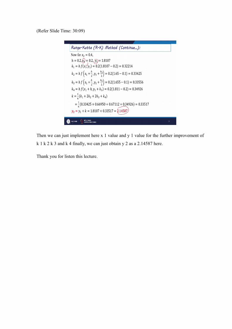
Then we can just implement here x 1 value and y 1 value for the further improvement of

k 1 k 2 k 3 and k 4 finally, we can just obtain y 2 as a 2.14587 here.

Thank you for listen this lecture.

Numerical Methods: Finite Difference Approach

Documents