Numerical Linear Algebra and Matrix Analysis Higham ...eprints.ma.man.ac.uk/2411/01/covered/MIMS_ep2015_103.pdf · Numerical Linear Algebra and Matrix Analysisy Nicholas J. Higham

Numerical Linear Algebra and Matrix Analysis

Higham, Nicholas J.

2015

MIMS EPrint: 2015.103

Manchester Institute for Mathematical SciencesSchool of Mathematics

The University of Manchester

Reports available from: http://eprints.maths.manchester.ac.uk/And by contacting: The MIMS Secretary

School of Mathematics

The University of Manchester

Manchester, M13 9PL, UK

ISSN 1749-9097

1

Numerical Linear Algebra andMatrix Analysis†

Nicholas J. Higham

Matrices are ubiquitous in applied mathematics.Ordinary differential equations (ODEs) and partial dif-ferential equations (PDEs) are solved numerically byfinite difference or finite element methods, which leadto systems of linear equations or matrix eigenvalueproblems. Nonlinear equations and optimization prob-lems are typically solved using linear or quadraticmodels, which again lead to linear systems.

Solving linear systems of equations is an ancient task,undertaken by the Chinese around 1AD, but the studyof matrices per se is relatively recent, originating withArthur Cayley’s 1858 “A Memoir on the Theory of Matri-ces”. Early research on matrices was largely theoret-ical, with much attention focused on the developmentof canonical forms, but in the 20th century the practi-cal value of matrices started to be appreciated. Heisen-berg used matrix theory as a tool in the developmentof quantum mechanics in the 1920s. Early proponentsof the systematic use of matrices in applied mathemat-ics included Frazer, Duncan, and Collar, whose 1938book Elementary Matrices and Some Applications toDynamics and Differential Equations emphasized theimportant role of matrices in differential equations andmechanics. The continued growth of matrices in appli-cations, together with the advent of mechanical andthen digital computing devices, allowing ever largerproblems to be solved, created the need for greaterunderstanding of all aspects of matrices from theoryto computation.

This article treats two closely related topics: matrixanalysis, which is the theory of matrices with a focuson aspects relevant to other areas of mathematics, andnumerical linear algebra (also called matrix computa-tions), which is concerned with the construction andanalysis of algorithms for solving matrix problems aswell as related topics such as problem sensitivity androunding error analysis.

Important themes that are discussed in this articleinclude the matrix factorization paradigm, the use ofunitary transformations for their numerical stability,

†. Author’s final version, before copy editing and cross-referencing,of: N. J. Higham. Numerical linear algebra and matrix analysis. In N. J.Higham, M. R. Dennis, P. Glendinning, P. A. Martin, F. Santosa, andJ. Tanner, editors, The Princeton Companion to Applied Mathematics,pages 263–281. Princeton University Press, Princeton, NJ, USA, 2015.

exploitation of matrix structure (such as sparsity, sym-

metry, and definiteness), and the design of algorithms

to exploit evolving computer architectures.

Throughout the article, uppercase letters are used for

matrices and lower case letters for vectors and scalars.

Matrices and vectors are assumed to be complex, unless

otherwise stated, andA∗ = (aji) denotes the conjugate

transpose of A = (aij). An unsubscripted norm ‖ · ‖denotes a general vector norm and the corresponding

subordinate matrix norm. Particular norms used here

are the 2-norm ‖ · ‖2 and the Frobenius norm ‖ · ‖F .

The notation “i = 1: n” means that the integer variable

i takes on the values 1,2, . . . , n.

1 Nonsingularity and Conditioning

Nonsingularity of a matrix is a key requirement in many

problems, such as in the solution of n linear equations

inn unknowns. For some classes of matrices, nonsingu-

larity is guaranteed. A good example is the diagonally

dominant matrices. The matrix A ∈ Cn×n is strictly

diagonally dominant by rows if∑j 6=i|aij| < |aii|, i = 1: n

and strictly diagonally dominant by columns if A∗ is

strictly diagonally dominant by rows. Any matrix that

is strictly diagonally dominant by rows or columns

is nonsingular (a proof can be obtained by applying

Gershgorin’s theorem in section 5.1).

Since data is often subject to uncertainty we wish

to gauge the sensitivity of problems to perturbations,

which is done using condition numbers. An appropriate

condition number for the matrix inverse is

limε→0

sup‖∆A‖6ε‖A‖

‖(A+∆A)−1 −A−1‖ε‖A−1‖ .

This expression turns out to equal κ(A) = ‖A‖‖A−1‖,which is called the condition number of A with respect

to inversion. This condition number occurs in many

contexts. For example, suppose A is contaminated

by errors and we perform a similarity transformation

X−1(A + E)X = X−1AX + F . Then ‖F‖ = ‖X−1EX‖ 6κ(X)‖E‖ and this bound is attainable for some E. Hence

the errors can be multiplied by a factor as large as

κ(X). We therefore prefer to carry out similarity and

other transformations with matrices that are well con-

ditioned , that is, ones for which κ(X) is close to its

lower bound of 1. By contrast, a matrix for which κ is

large is called ill conditioned. For any unitary matrix X,

2

κ2(X) = 1, so in numerical linear algebra transforma-tions by unitary or orthogonal matrices are preferredand usually lead to numerically stable algorithms.

In practice we often need an estimate of the matrixcondition number number κ(A) but do not wish to goto the expense of computing A−1 in order to obtainit. Fortunately, there are algorithms that can cheaplyproduce a reliable estimate of κ(A) once a factorizationof A has been computed.

Note that the determinant, det(A), is rarely com-puted in numerical linear algebra. Its magnitude givesno useful information about the conditioning of A, notleast because of its extreme behavior under scaling:det(αA) = αn det(A).

2 Matrix Factorizations

The method of Gaussian elimination (GE) for solvinga nonsingular linear system Ax = b of n equationsin n unknowns reduces the matrix A to upper trian-gular form and then solves for x by substitution. GEis typically described by writing down the equationsa(k+1)ij = a(k)ij − a

(k)ik a

(k)kj /a

(k)kk (and similarly for b) that

describe how the starting matrix A = A(1) = (a(1)ij )changes on each of the n − 1 steps of the elimina-tion in its progress towards upper triangular form U .Working at the element level in this way leads to a pro-fusion of symbols, superscripts, and subscripts thattend to obscure the mathematical structure and hin-der insights being drawn into the underlying process.One of the key developments in the last century wasthe recognition that it is much more profitable to workat the matrix level. Thus the basic equation above iswritten as A(k+1) = MkA(k), where Mk agrees with theidentity matrix except below the diagonal in the kthcolumn, where its (i, k) element is mik = −a(k)ik /a

(k)kk ,

i = k + 1: n. Recurring the matrix equation givesU := A(n) = Mn−1 . . .M1A. Taking theMk matrices overto the left-hand side leads, after some calculations, tothe equation A = LU , where L is unit lower triangular,with (i, k) elementmik. The prefix “unit” means that Lhas ones on the diagonal.

GE is therefore equivalent to factorizing the matrixA as the product of a lower triangular matrix and anupper triangular matrix—something that is not at allobvious from the element-level equations. Solving thelinear systemAx = b now reduces to the task of solvingthe two triangular systems Ly = b and Ux = y .

Interpreting GE as LU factorization separates thecomputation of the factors from the solution of the tri-

angular systems. It is then clear how to solve efficientlyseveral systems Axi = bi, i = 1: r , with different right-hand sides but the same coefficient matrix A: computethe LU factors once and then re-use them to solve foreach xi in turn.

This matrix factorization1 viewpoint dates fromaround the 1940s and has been extremely successfulin matrix computations. In general, a factorization is arepresentation of a matrix as a product of “simpler”matrices. Factorization is a tool that can be used tosolve a variety of problems, as we will see below.

Two particular benefits of factorizations are unityand modularity. GE, for example, can be organizedin several different ways, corresponding to differentorderings of the three nested loops that it comprises,as well as the use of different blockings of the matrixelements. Yet all of them compute the same LU factor-ization, carrying out the same mathematical operationsin a different order. Without the unifying concept of afactorization, reasoning about these GE variants wouldbe difficult.

Modularity refers to the way that a factorizationbreaks a problem down into separate tasks, which canbe analyzed or programmed independently. To carryout a rounding error analysis of GE we can analyze theLU factorization and the solution of the triangular sys-tems by substitution separately and then put the analy-ses together. The rounding error analysis of substitu-tion can be re-used in the many other contexts in whichtriangular systems arise.

An important example of the use of LU factoriza-tion is in iterative refinement. Suppose we have usedGE to obtain a computed solution x to Ax = b infloating-point arithmetic. If we form r = b − Ax andsolve Ae = r , then in exact arithmetic y = x + e isthe true solution. In computing e we can reuse the LUfactors of A, so obtaining y from x is inexpensive. Inpractice, the computation of r , e, and y is subject torounding errors so the computed y is not equal to x.But under suitable assumptions y will be an improvedapproximation and we can iterate this refinement pro-cess. Iterative refinement is particularly effective if rcan be computed using extra precision.

Two other key factorizations are:

• Cholesky factorization: for Hermitian positive def-inite A ∈ Cn×n, A = R∗R, where R is upper tri-angular with positive diagonal elements, and thisfactorization is unique.

1. Or decomposition—the two terms are essentially synonymous.

3

• QR factorization: for A ∈ Cm×n with m > n, A =QR where Q ∈ Cm×m is unitary (Q∗Q = Im) andR ∈ Cm×n is upper trapezoidal, that is, R =

[R10

]with R1 ∈ Cn×n upper triangular.

These two factorizations are related: if A ∈ Cm×n withm > n has full rank and A = QR is a QR factorization,in which without loss of generality we can assume thatR has positive diagonal, then A∗A = R∗R, so R is theCholesky factor of A∗A.

The Cholesky factorization can be computed by whatis essentially a symmetric and scaled version of GE. TheQR factorization can be computed in three main ways,one of which is the classical Gram–Schmidt orthogonal-ization. The most widely used method constructs Q asa product of Householder reflectors, which are unitarymatrices of the formH = I−2vv∗/(v∗v), where v is anonzero vector. Note that H is a rank 1 perturbation ofthe identity and since it is Hermitian and unitary it is itsown inverse, that is, it is involutory . The third approachbuildsQ as a product of Givens rotations, each of whichis a 2 × 2 matrix

[ c s−s c

]embedded into two rows and

columns of anm×m identity matrix, where (in the realcase) c2 + s2 = 1.

The Cholesky factorization helps us to make themost of the very desirable property of positive definite-ness. For example, supposeA is Hermitian positive def-inite and we wish to evaluate the scalar α = x∗A−1x.We can rewrite it as x∗(R∗R)−1x = (x∗R−1)(R−∗x) =z∗z, where z = R−∗x. So once the Cholesky factoriza-tion has been computed we need just one triangularsolve to compute α, and of course there is no need toexplicitly invert the matrix A.

A matrix factorization might involve a larger num-ber of factors: A = N1N2 . . . Nk, say. It is immediatethat AT = NTkN

Tk−1 . . . N

T1 . This factorization of the

transpose may have deep consequences in a particu-lar application. For example, the discrete Fourier trans-form is the matrix–vector product y = Fnx, wherethe n × n matrix Fn has (p, q) element exp(−2π i(p −1)(q − 1)/n); Fn is a complex, symmetric matrix. Thefast Fourier transform (FFT) is a way of evaluating y inO(n log2n) operations, as opposed to the O(n2) oper-ations that are required by a standard matrix–vectormultiplication. Many variants of the FFT have been pro-posed since the original 1965 paper by Cooley andTukey. It turns out that different FFT variants corre-spond to different factorizations of Fn with k = log2nsparse factors. Some of these methods correspond sim-ply to transposing the factorization in another method

(recall that FTn = Fn), though this was not realizedwhen the methods were developed. Transposition alsoplays an important role in automatic differentiation:the so-called reverse or adjoint mode can be obtainedby transposing a matrix factorization representation ofthe forward mode.

The factorizations described in this section are in“plain vanilla” form, but all have variants that incor-porate pivoting. Pivoting refers to row or column inter-changes carried out at each step of the factorization asit is computed, introduced either to ensure that the fac-torization succeeds and is numerically stable or to pro-duce a factorization with certain desirable propertiesusually associated with rank deficiency. For GE, partialpivoting is normally used: at the start of the kth stageof the elimination an elementa(k)rk of largest modulus inthe kth column below the diagonal is brought into the(k, k) (pivot) position by interchanging rows k and r .Partial pivoting avoids dividing by zero (if a(k)kk = 0 afterthe interchange then the pivot column is zero below thediagonal and the elimination step can be skipped). Moreimportantly, partial pivoting ensures numerical stabil-ity; see section 8. The overall effect of GE with partialpivoting is to produce an LU factorization PA = LU ,where P is a permutation matrix.

Pivoted variants of Cholesky factorization and QRfactorization take the form PTAP = R∗R and AP =Q[R0

], where P is a permutation matrix and R satisfies

the inequalities

|rkk|2 >j∑i=k|rij|2, j = k+ 1: n, k = 1: n.

If A is rank deficient then R has the form R =[R11 R120 0

]with R11 nonsingular, and the rank of A is the dimen-sion of R11. Equally importantly, when A is nearly rankdeficient this tends to be revealed by a small trailingdiagonal block of R.

A factorization of great importance in a wide vari-ety of applications is the singular value decomposition(SVD) of A ∈ Cm×n:

A = UΣV∗, Σ = diag(σ1, σ2, . . . , σp) ∈ Rm×n, (1)

where p = min(m,n), U ∈ Cm×m and V ∈ Cn×n areunitary, and the singular values σi satisfy σ1 > σ2 >· · · > σp > 0. For a square A (m = n), the 2-normcondition number is given by κ2(A) = σ1/σn.

The polar decomposition of A ∈ Cm×n with m > nis a factorization A = UH in which U ∈ Cm×n hasorthonormal columns andH ∈ Cn×n is Hermitian posi-tive semidefinite. The matrixH is unique and is given by

4

(A∗A)1/2, where the exponent 1/2 denotes the princi-pal square root, whileU is unique ifA has full rank. Thepolar decomposition generalizes to matrices the polarrepresentation z = r eiθ of a complex number. The Her-mitian polar factor H is also known as the matrix abso-lute value, |A|, and is much studied in matrix analysisand functional analysis.

One reason for the importance of the polar decom-position is that it provides an optimal way to orthogo-nalize a matrix: a result of Fan and Hoffman (1955) saysthat U is the nearest matrix with orthonormal columnsto A in any unitarily invariant norm (a unitarily invari-ant norm is one with the property that ‖UAV‖ = ‖A‖for any unitary U and V ; the 2-norm and the Frobe-nius norm are particular examples). In various appli-cations a matrix A ∈ Rn×n that should be orthogonaldrifts from orthogonality because of rounding or othererrors; replacing it by the orthogonal polar factor U isthen a good strategy.

The polar decomposition also solves the orthogonalProcrustes problem, for A,B ∈ Cm×n,

min{‖A− BQ‖F : Q ∈ Cn×n, Q∗Q = I

},

for which any solution Q is a unitary polar factor ofB∗A. This problem comes from factor analysis and mul-tidimensional scaling in statistics, where the aim is tosee whether two data sets A and B are the same up toan orthogonal transformation.

Either of the SVD and the polar decomposition canbe derived, or computed, from the other. Histori-cally, the SVD came first (Beltrami, in 1873), with thepolar decomposition three decades behind (Autonne,in 1902).

3 Distance to Singularity and Low-RankPerturbations

The question commonly arises of whether a given per-turbation of a nonsingular matrix A preserves nonsin-gularity. In a sense, this question is trivial. Recallingthat a square matrix is nonsingular when all its eigen-values are nonzero, and that the product of two matri-ces is nonsingular unless one of them is singular, fromA + ∆A = A(I + A−1∆A) we see that A + ∆A is non-singular as long as A−1∆A has no eigenvalue equal to−1. However, this is not an easy condition to check,and in practice we may not know ∆A but only a boundfor its norm. Since any norm of a matrix exceeds themodulus of every eigenvalue, a sufficient condition forA + ∆A to be nonsingular is that ‖A−1∆A‖ < 1, whichis certainly true if ‖A−1‖‖∆A‖ < 1. This condition can

be rewritten as the inequality ‖∆A‖/‖A‖ < κ(A)−1,where κ(A) = ‖A‖‖A−1‖ > 1 is the condition numberintroduced in section 1. It turns out that we can alwaysfind a perturbation ∆A such that A + ∆A is singularand ‖∆A‖/‖A‖ = κ(A)−1. It follows that the relativedistance to singularity

d(A) =min { ‖∆A‖/‖A‖ : A+∆A is singular } (2)

is given by d(A) = κ(A)−1. This reciprocal relationbetween problem conditioning and the distance to asingular problem (one with an infinite condition num-ber) is common to a variety of problems in linear alge-bra and control theory, as shown by James Demmel inthe 1980s.

We may want a more refined test for whether A+∆Ais nonsingular. To obtain one we will need to makesome assumptions about the perturbation. Supposethat ∆A has rank 1: ∆A = xy∗, for some vectors x andy . From the analysis above we know that A + ∆A willbe nonsingular if A−1∆A = A−1xy∗ has no eigenvalueequal to−1. Using the fact that the nonzero eigenvaluesof AB are the same as those of BA for any conformablematrices A and B, we see that the nonzero eigenvaluesof (A−1x)y∗ are the same as those of y∗A−1x. HenceA+ xy∗ is nonsingular as long as y∗A−1x 6= −1.

Now that we know when A+ xy∗ is nonsingular wemight ask if there is an explicit formula for the inverse.Since A + xy∗ = A(I + A−1xy∗) we can take A = Iwithout loss of generality. So we are looking for theinverse of B = I + xy∗. One way to find it is to guessthat B−1 = I + θxy∗ for some scalar θ and equate theproduct with B to I, to obtain θ(1+y∗x)+1 = 0. Thus(I +xy∗)−1 = I −xy∗/(1+y∗x). The correspondingformula for (A+ xy∗)−1 is

(A+ xy∗)−1 = A−1 −A−1xy∗A−1/(1+y∗A−1x),

which is known as the Sherman–Morrison formula.This formula and its generalizations originate in the1940s and have been rediscovered many times. Thecorresponding formula for a rank p perturbation isthe Sherman–Morrison–Woodbury formula: for U,V ∈Cn×p ,

(A+UV∗)−1 = A−1 −A−1U(I + V∗A−1U)−1V∗A−1.

Important applications of these formulae are in opti-mization, where rank-1 or rank-2 updates are made toHessian approximations in quasi-Newton methods andto basis matrices in the simplex method. More gener-ally, the task of updating the solution to a problem aftera coefficient matrix has undergone a low-rank change,or has had a row or column added or removed, arises in

5

many applications, including signal processing, where

new data is continually being received and old data is

discarded.

The minimal distance in the definition (2) of the dis-

tance to singularity d(A) can be shown to be attained

for a rank-1 matrix ∆A. Rank-1 matrices often feature

in the solutions of matrix optimization problems.

4 Computational Cost

In order to compare competing methods and predict

their practical efficiency we need to know their com-

putational cost. Traditionally, computational cost has

been measured by counting the number of scalar arith-

metic operations and retaining only the highest order

terms in the total. For example, using GE we can solve

a system of n linear equations in n unknowns with

n3/3+O(n2) additions, n3/3+O(n2)multiplications,

and O(n) divisions. This is typically summarized as

2n3/3 flops, where a flop denotes any of the scalar

operations +,−,∗, /. Most standard problems involv-

ing n×nmatrices can be solved with a cost of order n3

flops or less, so the interest is in the exponent (1, 2, or 3)

and the constant of the dominant term. However, the

costs of moving data around a computer’s hierarchi-

cal memory and the costs of communicating between

different processors on a multiprocessor system can

be equally important. Simply counting flops does not

therefore necessarily give a good guide to performance

in practice.

Seemingly trivial problems can offer interesting chal-

lenges as regards minimizing arithmetic costs. For

matrices A, B, and C of any dimensions such that the

product ABC is defined, how should we compute the

product? The associative law for matrix multiplication

tells us that (AB)C = A(BC), but this mathematical

equivalence is not a computational one. To see why,

note that for three vectors a,b, c ∈ Rn we can write

(ab∗)︸ ︷︷ ︸n×n

c = a(b∗c)︸ ︷︷ ︸1×1

.

Evaluation of the left-hand side requiresO(n2) flops, as

there is an outer product ab∗ and then a matrix–vector

product to evaluate, while evaluation of the right-hand

side requires just O(n) flops, as it involves only vec-

tor operations: an inner product and a vector scaling.

One should always be alert for opportunities to use the

associative law to save computational effort.

5 Eigenvalue Problems

The eigenvalue problem Ax = λx for a square matrixA ∈ Cn×n, which seeks an eigenvalue λ ∈ C and aneigenvector x 6= 0, arises in many forms. Depending onthe application we may want all the eigenvalues or justa subset, such as the 10 that have the largest real part,and eigenvectors may or may not be required as well.Whether the problem is Hermitian or non-Hermitianchanges its character greatly. In particular, while a Her-mitian matrix has real eigenvalues and a linearly inde-pendent set of n eigenvectors that can be taken tobe orthonormal, the eigenvalues of a non-Hermitianmatrix can be anywhere in the complex plane and theremay not be a set of eigenvectors that spans Cn.

5.1 Bounds and Localization

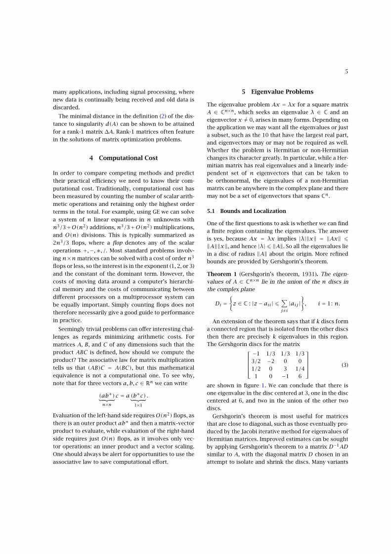
One of the first questions to ask is whether we can finda finite region containing the eigenvalues. The answeris yes, because Ax = λx implies |λ|‖x‖ = ‖Ax‖ 6‖A‖‖x‖, and hence |λ| 6 ‖A‖. So all the eigenvalues liein a disc of radius ‖A‖ about the origin. More refinedbounds are provided by Gershgorin’s theorem.

Theorem 1 (Gershgorin’s theorem, 1931). The eigen-values of A ∈ Cn×n lie in the union of the n discs inthe complex plane

Di ={z ∈ C : |z − aii| 6

∑j 6=i|aij|

}, i = 1: n.

An extension of the theorem says that if k discs forma connected region that is isolated from the other discsthen there are precisely k eigenvalues in this region.The Gershgorin discs for the matrix

−1 1/3 1/3 1/33/2 −2 0 01/2 0 3 1/41 0 −1 6

(3)

are shown in figure 1. We can conclude that there isone eigenvalue in the disc centered at 3, one in the disccentered at 6, and two in the union of the other twodiscs.

Gershgorin’s theorem is most useful for matricesthat are close to diagonal, such as those eventually pro-duced by the Jacobi iterative method for eigenvalues ofHermitian matrices. Improved estimates can be soughtby applying Gershgorin’s theorem to a matrix D−1ADsimilar to A, with the diagonal matrix D chosen in anattempt to isolate and shrink the discs. Many variants

6

−4 −3 −2 −1 0 1 2 3 4 5 6 7 8−2

−1

0

1

2

• • • •

Figure 1 Gershgorin discs for the matrix in (3); theeigenvalues are marked as solid dots.

of Gershgorin’s theorem exist with discs replaced byother shapes.

The spectral radius ρ(A) (the largest absolute valueof any eigenvalue of A) satisfies ρ(A) 6 ‖A‖, as shownabove, but this inequality can be arbitrarily weak, asthe matrix

[1 θ0 1

]shows for |θ| � 1. It is natural to ask

whether there are any sharper relations between thespectral radius and norms. One answer is the equality

ρ(A) = limk→∞

‖Ak‖1/k. (4)

Another is the result that given any ε > 0 there is anorm such that ‖A‖ 6 ρ(A) + ε; however, the normdepends onA. This result can be used to give a proof ofthe fact, discussed in the article on the Jordan canonicalform, that the powers ofA converge to zero if ρ(A) < 1.

The field of values, also known as the numericalrange, is a tool that can be used for localization andmany other purposes. It is defined for A ∈ Cn×n by

F(A) ={z∗Azz∗z

: 0 6= z ∈ Cn}.

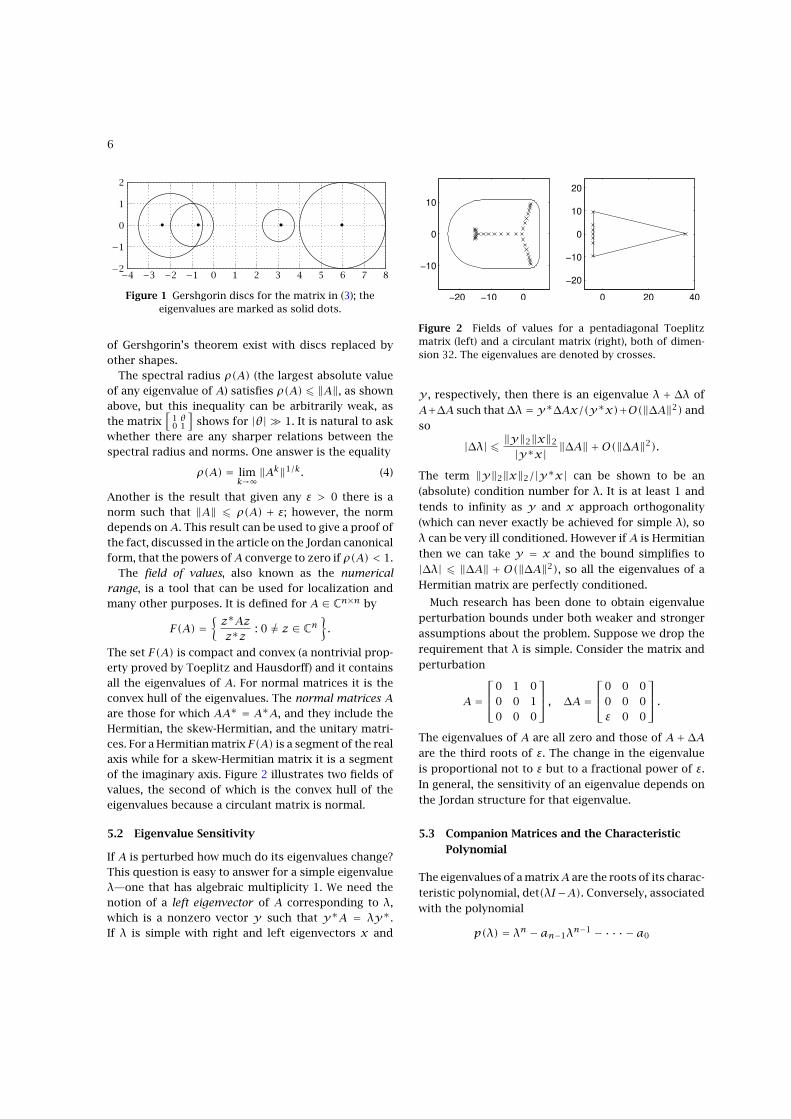
The set F(A) is compact and convex (a nontrivial prop-erty proved by Toeplitz and Hausdorff) and it containsall the eigenvalues of A. For normal matrices it is theconvex hull of the eigenvalues. The normal matrices Aare those for which AA∗ = A∗A, and they include theHermitian, the skew-Hermitian, and the unitary matri-ces. For a Hermitian matrix F(A) is a segment of the realaxis while for a skew-Hermitian matrix it is a segmentof the imaginary axis. Figure 2 illustrates two fields ofvalues, the second of which is the convex hull of theeigenvalues because a circulant matrix is normal.

5.2 Eigenvalue Sensitivity

If A is perturbed how much do its eigenvalues change?This question is easy to answer for a simple eigenvalueλ—one that has algebraic multiplicity 1. We need thenotion of a left eigenvector of A corresponding to λ,which is a nonzero vector y such that y∗A = λy∗.If λ is simple with right and left eigenvectors x and

−20 −10 0

−10

0

10

0 20 40

−20

−10

0

10

20

Figure 2 Fields of values for a pentadiagonal Toeplitzmatrix (left) and a circulant matrix (right), both of dimen-sion 32. The eigenvalues are denoted by crosses.

y , respectively, then there is an eigenvalue λ + ∆λ of

A+∆A such that∆λ = y∗∆Ax/(y∗x)+O(‖∆A‖2) and

so

|∆λ| 6 ‖y‖2‖x‖2

|y∗x| ‖∆A‖ +O(‖∆A‖2).

The term ‖y‖2‖x‖2/|y∗x| can be shown to be an

(absolute) condition number for λ. It is at least 1 and

tends to infinity as y and x approach orthogonality

(which can never exactly be achieved for simple λ), so

λ can be very ill conditioned. However if A is Hermitian

then we can take y = x and the bound simplifies to

|∆λ| 6 ‖∆A‖ + O(‖∆A‖2), so all the eigenvalues of a

Hermitian matrix are perfectly conditioned.

Much research has been done to obtain eigenvalue

perturbation bounds under both weaker and stronger

assumptions about the problem. Suppose we drop the

requirement that λ is simple. Consider the matrix and

perturbation

A =

0 1 00 0 10 0 0

, ∆A =

0 0 00 0 0ε 0 0

.The eigenvalues of A are all zero and those of A+ ∆Aare the third roots of ε. The change in the eigenvalue

is proportional not to ε but to a fractional power of ε.In general, the sensitivity of an eigenvalue depends on

the Jordan structure for that eigenvalue.

5.3 Companion Matrices and the Characteristic

Polynomial

The eigenvalues of a matrixA are the roots of its charac-

teristic polynomial, det(λI−A). Conversely, associated

with the polynomial

p(λ) = λn − an−1λn−1 − · · · − a0

7

is the companion matrix

C =

an−1 an−2 . . . . . . a0

1 0 . . . . . . 0

0 1. . . 0

.... . . 0

...0 . . . . . . 1 0

,

and the eigenvalues of C are the roots of p.This relation means that the roots of a polynomial

can be found by computing the eigenvalues of an n×nmatrix, and this approach is used by some computercodes, for example the roots function of MATLAB.While standard eigenvalue algorithms do not exploitthe structure of C , this approach has proved competi-tive with specialist polynomial root-finding algorithms.Another use for the relation is to obtain bounds forroots of polynomials from bounds for matrix eigen-values, and vice versa.

Companion matrices have many interesting proper-ties. For example, any nonderogatory n × n matrixis similar to a companion matrix. Companion matri-ces therefore have featured strongly in matrix analysisand also in control theory. However, similarity trans-formations to companion form are little used in prac-tice because of problems with ill conditioning andnumerical instability.

Returning to the characteristic polynomial, p(λ) =det(λI −A) = λn −an−1λn−1 − · · · −a0, we know thatp(λi) = 0 for every eigenvalue λi of A. The Cayley–Hamilton theorem says that p(A) = An − an−1An−1 −· · · − a0I = 0 (which cannot be obtained simply byputting “λ = A” in the previous expression!). Hence thenth power of A, and inductively all higher powers, areexpressible as a linear combination of I, A, . . . , An−1.Moreover, if A is nonsingular then from A−1p(A) = 0 itfollows that A−1 can also be written as a polynomial inA of degree at most n− 1. These relations are not use-ful for practical computation because the coefficientsai can vary tremendously in magnitude and it is notpossible to compute them to high relative accuracy.

5.4 Eigenvalue Inequalities for Hermitian Matrices

The eigenvalues of Hermitian matrices A ∈ Cn×n,which in this section we order λn 6 · · · 6 λ1, satisfymany beautiful inequalities. Among the most impor-tant are those in the Courant–Fischer theorem (1905),which states that every eigenvalue is the solution of amin-max problem over a suitable subspace S of Cn:

λi = mindim(S)=n−i+1

max06=x∈S

x∗Axx∗x

.

Special cases are λn = minx 6=0 x∗Ax/(x∗x) and λ1 =maxx 6=0 x∗Ax/(x∗x).

Takingx to be a unit vector ei in the previous formulafor λ1 gives λ1 > aii for all i. This inequality is justthe first in a sequence of inequalities relating sums ofeigenvalues to sums of diagonal elements, obtained bySchur in 1923:

k∑i=1

λi >k∑i=1

aii, k = 1: n, (5)

where {aii} is the set of diagonal elements of Aarranged in decreasing order: a11 > · · · > ann. Thereis equality for k = n, since both sides equal trace(A).These inequalities say that the vector [λ1, . . . , λn] ofeigenvalues majorizes the vector [a11, . . . , ann] of diag-onal elements.

In general there is no useful formula for the eigen-values of a sum A + B of Hermitian matrices. How-ever, the Courant–Fischer theorem yields the upper andlower bounds

λk(A)+ λn(B) 6 λk(A+ B) 6 λk(A)+ λ1(B),

from which it follows that |λk(A + B) − λk(A)| 6max(|λn(B)|, |λ1(B)|) = ‖B‖2. The latter inequalityagain shows that the eigenvalues of a Hermitian matrixare well conditioned under perturbation.

The Cauchy interlace theorem has a different flavor. Itrelates the eigenvalues of successive leading principalsubmatrices Ak = A(1: k,1: k) by

λk+1(Ak+1) 6 λk(Ak) 6 λk(Ak+1)

6 · · · 6 λ2(Ak+1) 6 λ1(Ak) 6 λ1(Ak+1)

for k = 1: n − 1, showing that the eigenvalues of Akinterlace those of Ak+1.

In 1962 Alfred Horn made a conjecture that a cer-tain set of linear inequalities involving real numbersαi, βi, and γi, i = 1: n, is necessary and sufficient forthe existence of n× n Hermitian matrices A, B, and Cwith eigenvalues the αi, βi, and γi, respectively, suchthat C = A+B. The conjecture was open for many yearsbut was finally proved to be true in papers published byKlyachko in 1998 and Knutson and Tao in 1999, whichexploit deep connections with algebraic geometry, rep-resentations of Lie groups, and quantum cohomology.

5.5 Solving the Non-Hermitian Eigenproblem

The simplest method for computing eigenvalues, thepower method, computes just one: the largest in mod-ulus. It comprises repeated multiplication of a starting

8

vector x by A. Since the resulting sequence is liable tooverflow or underflow in floating-point arithmetic onenormalizes the vector after each iteration. Thereforeone step of the power method has the form x ← Ax,x ← ν−1x, where ν = xj with |xj| = maxi |xi|. If Ahas a unique eigenvalue λ of largest modulus and thestarting vector has a component in the direction of thecorresponding eigenvector then ν converges to λ and xconverges to the corresponding eigenvector. The powermethod is most often applied to (A−µI)−1, where µ isan approximation to an eigenvalue of interest. In thisform it is known as inverse iteration and convergence isto the eigenvalue closest to µ. We now turn to methodsthat compute all the eigenvalues.

Since similarities X−1AX preserve the eigenvaluesand change the eigenvectors in a controlled way, car-rying out a sequence of similarity transformations toreduceA to a simpler form is a natural way to tackle theeigenproblem. Some early methods used nonunitary X,but such transformations are now avoided because ofnumerical instability when X is ill conditioned. Sincethe 1960s the focus has been on using unitary similar-ities to compute the Schur decomposition A = QTQ∗,where Q is unitary and T is upper triangular. The diag-onal entries of T are the eigenvalues of A, and they canbe made to appear in any order by appropriate choice ofQ. The first k columns ofQ span an invariant subspacecorresponding to the eigenvalues t11, . . . , tkk. Eigen-vectors can be obtained by solving triangular systemsinvolving T .

For some matrices the Schur factor T is diagonal;these are precisely the normal matrices defined in sec-tion 5.1. The real Schur decomposition contains onlyreal matrices when A is real: A = QRQT , where Q isorthogonal and R is real upper quasi-triangular, whichmeans that R is upper triangular except for 2×2 blockson the diagonal corresponding to complex conjugateeigenvalues.

The standard algorithm for solving the non-Hermitian eigenproblem is the QR algorithm, whichwas proposed independently by John Francis and VeraKublanovskaya in 1961. The matrix A ∈ Cn×n isfirst unitarily reduced to upper Hessenberg form H =U∗AU (hij = 0 for i > j + 1), with U a product ofHouseholder matrices. The QR iteration constructs asequence of upper Hessenberg matrices beginning withH1 = H defined by Hk−µkI =: QkRk (QR factorization,computed using Givens rotations),Hk+1 := RkQk+µkI,where the µk are shifts chosen to accelerate the con-vergence of Hk to upper triangular form. It is easy to

check that Hk+1 = Q∗kHkQk, so the QR iteration carries

out a sequence of unitary similarity transformations.

Why the QR iteration works is not obvious but can

be elegantly explained by analyzing the subspaces

spanned by the columns of Qk. To produce a practi-

cal and efficient algorithm various refinements of the

iteration are needed, which include

• deflation, whereby when an element on the first

subdiagonal of Hk becomes small, that element is

set to zero and the problem is split into two smaller

problems that are solved independently,

• a double shift technique for real A that allows

two QR steps with complex conjugate shifts to be

carried out entirely in real arithmetic and gives

convergence to the real Schur form,

• a multishift technique for including m different

shifts in a single QR iteration.

A proof of convergence is lacking for all current shift

strategies. Implementations introduce a random shift

when convergence appears to be stagnating. The QR

algorithm works very well in practice and continues

to be the method of choice for the non-Hermitian

eigenproblem.

5.6 Solving the Hermitian Eigenproblem

The eigenvalue problem for Hermitian matrices is eas-

ier to solve than that for non-Hermitian matrices and

the range of available numerical methods is much

wider.

To solve the complete Hermitian eigenproblem we

need to compute the spectral decomposition A =QDQ∗, where D = diag(λi) contains the eigenvalues

and the columns of the unitary matrix Q are the corre-

sponding eigenvectors. Many methods begin by unitary

reduction to tridiagonal form T = U∗AU , where tij = 0

for |i− j| > 1 and the unitary matrix U is constructed

as a product of Householder matrices. The eigenvalue

problem for T is much simpler, though still nontriv-

ial. The most widely used method is the QR algorithm,

which has the same form as in the non-Hermitian case

but with the upper Hessenberg Hk replaced by the Her-

mitian tridiagonal Tk and the shifts chosen to acceler-

ate the convergence of Tk to diagonal form. The Her-

mitian QR algorithm with appropriate shifts has been

proved to converge at a cubic rate.

Another method for solving the Hermitian tridiag-

onal eigenproblem is the divide and conquer method .

9

This method decouples T in the form

T =[T11 0

0 T22

]+αvv∗,

where only the trailing diagonal element of T11 and theleading diagonal element of T22 differ from the corre-sponding elements of T and hence the vector v hasonly two nonzero elements. The eigensystems of T11

and T22 are found by applying the method recursively,yielding T11 = Q1Λ1Q∗1 and T22 = Q2Λ2Q∗2 . Then

T =[Q1Λ1Q∗1 0

0 Q2Λ2Q∗2

]+αvv∗

= diag(Q1,Q2)(diag(Λ1,Λ2)+αvv∗

)diag(Q1,Q2)∗,

where v = diag(Q1,Q2)∗v . The eigensystem of a rank-1 perturbed diagonal matrix D+ρzz∗ can be found bysolving the secular equation obtained by equating thecharacteristic polynomial to zero:

f(λ) = 1+ ρn∑j=1

|zj|2djj − λ

= 0.

Putting the pieces together yields the overall eigende-composition.

Other methods are suitable for computing just a por-tion of the spectrum. Suppose we want to compute thekth smallest eigenvalue of T and that we can some-how compute the integer N(x) equal to the numberof eigenvalues of T that are less than or equal to x.Then we can apply the bisection method to N(x) tofind the point where N(x) jumps from k − 1 to k.We can compute N(x) by making use of the followingresult about the inertia of a Hermitian matrix, definedby inertia(A) = (ν, ζ,π), where ν is the number of neg-ative eigenvalues, ζ is the number of zero eigenvalues,and π is the number of positive eigenvalues.

Theorem 2 (Sylvester’s inertia theorem). If A is Her-mitian and M is nonsingular then inertia(A) =inertia(M∗AM).

Sylvester’s inertia theorem says that the numberof negative, zero, and positive eigenvalues does notchange under congruence transformations. By using GEwe can factorize2 T − xI = LDL∗, where D is diago-nal and L is unit lower bidiagonal (a bidiagonal matrixis one that is both triangular and tridiagonal). Theninertia(T − xI) = inertia(D), so the number of nega-tive diagonal or zero elements of D equals the numberof eigenvalues of T − xI less than or equal to 0, whichis the number of eigenvalues of T less than or equal

2. The factorization may not exist, but if it does not we can simplyperturb T slightly and try again without any loss of numerical stability.

to x, that is, N(x). The LDL∗ factors of a tridiagonal

matrix can be computed in O(n) flops, so this bisec-

tion process is efficient. An alternative approach can be

built by using properties of Sturm sequences, which are

sequences comprising the characteristic polynomials

of leading principal submatrices of T − λI.

5.7 Computing the SVD

For a rectangular matrix A ∈ Cm×n the eigenvalues of

the Hermitian matrix[

0 AA∗ 0

]of dimension m + n are

plus and minus the nonzero singular values of A along

with m + n − 2 min(m,n) zeros. Hence the SVD can

be computed via the eigendecomposition of this larger

matrix. However, this would be inefficient, and instead

one uses algorithms that work directly on A and are

analogues of the algorithms for Hermitian matrices.

The standard approach is to reduce A to bidiagonal

form B by Householder transformations applied on the

left and the right and then to apply an adaptation of the

QR algorithm that works on the bidiagonal factor (and

implicitly applies the QR algorithm to the tridiagonal

matrix B∗B).

5.8 Generalized Eigenproblems

The generalized eigenvalue problem (GEP) Ax = λBx,

with A,B ∈ Cn×n, can be converted into a standard

eigenvalue problem if B (say) is nonsingular: B−1Ax =λx. However, such a transformation is inadvisable

numerically unless B is very well conditioned. IfA and Bhave a common null vector z the problem takes on a dif-

ferent character because then (A−λB)z = 0 for any λ;

such a problem is called singular . We will assume that

the problem is regular , so that det(A − λB) 6≡ 0. The

linear polynomial A− λB is sometimes called a pencil .

It is convenient to write λ = α/β, where α and β are

not both zero, and rephrase the problem in the more

symmetric form βAx = αBx. If x is a nonzero vector

such that Bx = 0 then, since the problem is assumed

to be regular, Ax 6= 0 and so β = 0. This means that

λ = ∞ is an eigenvalue. Infinite eigenvalues may seem

a strange concept, but in fact they are no different in

most respects to finite eigenvalues.

An important special case is the definite general-

ized eigenvalue problem, in which A and B are Hermi-

tian and B (say) is positive definite. If B = R∗R is a

Cholesky factorization then Ax = λBx can be rewrit-

ten as R−∗AR−1 ·Rx = λRx, which is a standard eigen-

problem for the Hermitian matrix C = R−∗AR−1. This

10

argument shows that the eigenvalues of a definite prob-lem are all real. Definite generalized eigenvalue prob-lems arise in many physical situations where an energyminimization principle is at work, such as in problemsin engineering and physics.

A generalization of the QR algorithm called the QZalgorithm computes a generalization to two matricesof the Schur decomposition: Q∗AZ = T , Q∗BZ = S,where Q and Z are unitary and T and S are upper tri-angular. The generalized Schur decomposition yieldsthe eigenvalues as the ratios tii/sii and enables eigen-vectors to be computed by substitution.

The quadratic eigenvalue problem (QEP) Q(λ)x =(λ2A2 + λA1 + A0)x = 0, where Ai ∈ Cn×n, i = 0: 2,arises most commonly in the dynamic analysis of struc-tures when the finite element method is used to dis-cretize the original PDE into a system of second-orderODEs A2q(t) + A1q(t) + A0q(t) = f(t). Here, the Aiare usually Hermitian (though A1 is skew-Hermitian ingyroscopic systems) and positive (semi)definite. Anal-ogously to the GEP, the QEP is said to be regular ifdet(Q(λ)) 6≡ 0. The quadratic problem differs funda-mentally from the linear GEP because a regular problemhas 2n eigenvalues, which are the roots of det(Q(λ)) =0, but at most n linearly independent eigenvectors,and a vector may be an eigenvector for two differenteigenvalues. For example, the QEP with

Q(λ) = λ2I + λ[−1 −6

2 −9

]+[

0 12−2 14

]has eigenvalues 1, 2, 3, and 4, with eigenvectors

[10

],[

01

],[

11

], and

[11

], respectively. Moreover, there is no

Schur form for three or more matrices, that is, we can-not in general find unitary matrices U and V such thatU∗AiV is triangular for i = 0: 2.

Associated with the QEP is the matrixQ(X) = A2X2+A1X +A0, with X ∈ Cn×n. From the relation

Q(λ)−Q(X) = A2(λ2I −X2)+A1(λI −X)= (λA2 +A2X +A1)(λI −X)

it is clear that if we can find a matrix X such thatQ(X) = 0, known as a solvent, then we have reducedthe QEP to finding the eigenvalues of X and solvingone n×n GEP. For the 2×2 Q above there are five sol-vents, one of which is

[3 01 2

]. The existence and enumer-

ation of solvents is nontrivial and leads into the theoryof matrix polynomials. In general, matrix polynomialsare matrices of the form

∑ki=0 λiAi whose elements are

polynomials in a complex variable; an older term forsuch matrices is λ-matrices.

The standard approach for numerical solution of theQEP mimics the conversion of the scalar polynomialroot problem into a matrix eigenproblem described insection 5.3. From the relation

L(λ)z ≡([A1 A0

I 0

]+ λ

[A2 00 −I

])[λxx

]=[Q(λ)x

0

]we see that the eigenvalues of the quadratic Q are theeigenvalues of the 2n×2n linear polynomial L(λ). Thisis an example of an exact linearization process—thanksto the hidden λ in the eigenvector! The eigenvalues of Lcan be found using the QZ algorithm. The eigenvectorsof L have the form z =

[ λxx], where x is an eigenvector

of Q, and so x can be obtained from either the first n(if λ 6= 0) or the last n components of z.

6 Sparse Linear Systems

For linear systems coming from discretization of dif-ferential equations it is common that A is banded ,that is, the nonzero elements lie in a band about themain diagonal. An extreme case is a tridiagonal matrix,of which the classic example is the second-differencematrix, illustrated for n = 4 by

A =

−2 1 0 0

1 −2 1 0

0 1 −2 1

0 0 1 −2

, A−1 = −15

4 3 2 13 6 4 22 4 6 31 2 3 4

.This matrix corresponds to a centered finite differenceapproximation to a second derivative: f ′′(x) ≈ (f (x +h)−2f(x)+f(x−h))/h2. Note thatA−1 is a full matrix.For banded matrices, GE produces banded LU factorsand its computational cost is proportional to n timesthe square of the bandwidth.

A matrix is sparse if advantage can be taken of thezero entries, because of either their number or their dis-tribution. A banded matrix is a special case of a sparsematrix. Sparse matrices are stored on a computer not asa square array but in a special format that records onlythe nonzeros and their location in the matrix. This canbe done with three vectors: one to store the nonzeroentries and the other two to define the row and columnindices of the elements in the first vector.

Sparse matrices help to explain the tenet: never solvea linear system Ax = b by computing x = A−1 ×b. Thereasons for eschewing A−1 are threefold:

• Computing A−1 requires three times as many flopsas solving Ax = b by GE with partial pivoting.

11

• GE with partial pivoting is backward stable for solv-ing Ax = b (see section 8) but solution via A−1 isnot.

• IfA is sparse,A−1 is generally dense and so requiresmuch more storage than GE with partial pivoting.

When GE is applied to a sparse matrix fill-in occurswhen the row operations cause a zero entry to becomenonzero during the elimination. To minimize the stor-age and the computational cost, fill-in must be avoidedas much as possible. This can be done by employingrow and column interchanges to choose a suitable pivotfrom the active submatrix. The first such strategy wasintroduced by Markowitz in 1957. At the kth stage,with c(k)j denoting the number of nonzeros in rowsk to n of column j and r (k)i the number of nonzerosin columns k to n of row i, the Markowitz strategyfinds the pair (r , s) that minimizes

(r (k)i − 1

)(c(k)j − 1

)over all nonzero potential pivots a(k)ij and then takesa(k)rs as the pivot. The quantity being minimized is abound on the fill-in. In practice, the potential pivotsmust be restricted to those not too much smaller inmagnitude than the partial pivot, in order to preservenumerical stability. The result of GE with Markowitzpivoting is a factorization PAQ = LU , where P and Qare permutation matrices.

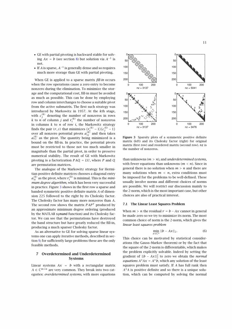
The analogue of the Markowitz strategy for Hermi-tian positive definite matrices chooses a diagonal entrya(k)ii as the pivot, where r (k)i is minimal. This is the mini-mum degree algorithm, which has been very successfulin practice. Figure 3 shows in the first row a sparse andbanded symmetric positive definite matrix A of dimen-sion 225 followed to the right by its Cholesky factor.The Cholesky factor has many more nonzeros than A.The second row shows the matrix PAPT produced byan approximate minimum degree ordering (producedby the MATLAB symamd function) and its Cholesky fac-tor. We can see that the permutations have destroyedthe band structure but have greatly reduced the fill-in,producing a much sparser Cholesky factor.

As an alternative to GE for solving sparse linear sys-tems one can apply iterative methods, described in sec-tion 9; for sufficiently large problems these are the onlyfeasible methods.

7 Overdetermined and UnderdeterminedSystems

Linear systems Ax = b with a rectangular matrixA ∈ Cm×n are very common. They break into two cat-egories: overdetermined systems, with more equations

0 100 200

0

50

100

150

200

nz = 3137

0 100 200

0

50

100

150

200

nz = 5041

0 100 200

0

50

100

150

200

nz = 3137

0 100 200

0

50

100

150

200

nz = 3476

Figure 3 Sparsity plots of a symmetric positive definitematrix (left) and its Cholesky factor (right) for originalmatrix (first row) and reordered matrix (second row). nz isthe number of nonzeros.

than unknowns (m > n), and underdetermined systems,with fewer equations than unknowns (m < n). Since ingeneral there is no solution whenm > n and there aremany solutions when m < n, extra conditions mustbe imposed for the problems to be well-defined. Theseusually involve norms and different choices of normsare possible. We will restrict our discussion mainly tothe 2-norm, which is the most important case, but otherchoices are also of practical interest.

7.1 The Linear Least Squares Problem

Whenm > n the residual r = b−Ax cannot in generalbe made zero so we try to minimize its norm. The mostcommon choice of norm is the 2-norm, which gives thelinear least squares problem

minx∈Cn

‖b −Ax‖2. (6)

This choice can be motivated by statistical consider-ations (the Gauss–Markov theorem) or by the fact thatthe square of the 2-norm is differentiable, which makesthe problem explicitly solvable. Indeed by setting thegradient of ‖b − Ax‖2

2 to zero we obtain the normalequations A∗Ax = A∗b, which any solution of the leastsquares problem must satisfy. If A has full rank thenA∗A is positive definite and so there is a unique solu-tion, which can be computed by solving the normal

12

equations using Cholesky factorization. For reasons ofnumerical stability, it is preferable to use a QR fac-torization: if A = Q

[R10

]then the normal equations

reduce to the triangular system R1x = c, where c is thefirst n components of Q∗b.

WhenA is rank deficient there are many least squaressolutions, which vary widely in norm. A natural choiceis one of minimal 2-norm, and in fact there is a uniqueminimal 2-norm solution, xLS , given by

xLS =r∑i=1

(u∗i b/σi)vi,

where

A = UΣV∗, U = [u1, . . . , um], V = [v1, . . . , vn] (7)

is an SVD and r = rank(A). The use of this formula inpractice is not straightforward because a matrix storedin floating-point arithmetic will rarely have any zerosingular values. Therefore r must be chosen by desig-nating which singular values can be regarded as negligi-ble and this choice should take account of the accuracywith which the elements of A are known.

Another choice of least squares solution in the rank-deficient case is a basic solution: one with at most rnonzeros. Such a solution can be computed via the QRfactorization with column pivoting.

7.2 Underdetermined Systems

When m < n and A has full rank, there are infinitelymany solutions to Ax = b and again it is natural toseek one of minimal 2-norm. There is a unique suchsolution xLS = A∗(AA∗)−1b, and it is best computedvia a QR factorization, this time of A∗. A basic solu-tion, with m nonzeros, can alternatively be computed.As a simple example, consider the problem “find twonumbers whose sum is 5”, that is, solve [1 1]

[ x1x2

]=

5. A basic solution is [5 0]T while the minimal 2-norm solution is [5/2 5/2]T . Minimal 1-norm solu-tions to underdetermined systems are important incompressed sensing.

7.3 Pseudoinverse

The analysis in the previous two subsections can beunified in a very elegant way by making use of theMoore–Penrose pseudoinverse A+ of A ∈ Cm×n, whichis defined as the unique X ∈ Cn×m satisfying theMoore–Penrose conditions

AXA = A, XAX = X,(AX)∗ = AX, (XA)∗ = XA.

(It is certainly not obvious that these equations havea unique solution.) In the case where A is square andnonsingular it is easily seen that A+ is just A−1. More-over, if rank(A) = n then A+ = (A∗A)−1A∗, while ifrank(A) = m then A+ = A∗(AA∗)−1. In terms of theSVD (7),

A+ = V diag(σ−11 , . . . , σ−1

r ,0, . . . ,0)U∗,

where r = rank(A). The formula xLS = A+b holds forall m and n, so the pseudoinverse yields the minimal2-norm solution to both the least squares (overdeter-mined) problem Ax = b and an underdetermined sys-tem Ax = b. The pseudoinverse has many interestingproperties, including (A+)+ = A, but it is not alwaystrue that (AB)+ = B+A+.

Although the pseudoinverse is a very useful theoret-ical tool it is rarely necessary to compute it explicitly(just as for its special case the matrix inverse).

The pseudoinverse is just one of many ways of gen-eralizing the notion of inverse to rectangular matri-ces, but it is the right one for minimum 2-norm solu-tions to linear systems. Other generalized inverses canbe obtained by requiring only a subset of the fourMoore–Penrose conditions to hold.

8 Numerical Considerations

Prior to the introduction of the first digital comput-ers in the 1940s, numerical computations were carriedout by humans, sometimes with the aid of mechanicalcalculators. The human involvement in a sequence ofcalculations meant that potentially dangerous eventssuch as dividing by a tiny number or subtracting twonumbers that agree to almost all their significant digitscould be observed, their effect monitored, and possiblecorrective action taken—such as temporarily increas-ing the precision of the calculations. On the very earlycomputers intermediate results were observed on acathode-ray tube monitor, but this became impossibleas problem sizes increased (along with available com-puting power). Fears were raised in the 1940s that algo-rithms such as GE would suffer exponential growthof errors as the problem dimension increased, dueto the rapidly increasing number of arithmetic opera-tions, each having its associated rounding error. Thesefears were particularly concerning given that the errorgrowth might be unseen and unsuspected.

The subject of rounding error analysis grew outof the need to understand the effect on algorithmsof rounding errors. The person who did the most to

13

develop the subject was James Wilkinson, whose influ-ential papers and 1961 and 1965 books showed howbackward error analysis can be used to obtain deepinsights into numerical stability. We will discuss justtwo particular examples.

Wilkinson showed that when a nonsingular linearsystem Ax = b is solved by GE in floating-pointarithmetic the computed solution x satisfies

(A+∆A)x = b, ‖∆A‖∞ 6 p(n)ρnu‖A‖∞.

Here p(n) is a cubic polynomial, the growth factor

ρn =maxi,j,k |a(k)ij |maxi,j |aij|

> 1

measures the growth of elements during the elimina-tion, and u is the unit roundoff. This is a backwardstability result : it says that the computed solution xis the exact solution of a perturbed system. Ideally,we would like ‖∆A‖∞ 6 u‖A‖∞, which reflects theuncertainty caused by converting the elements of A tofloating-point numbers. The polynomial term p(n) ispessimistic and might be more realistically replaced byits square root. The danger term is the growth factorρn,and the conclusion from Wilkinson’s analysis is that apivoting strategy should aim to keep ρn small. If nopivoting is done, ρn can be arbitrarily large (e.g., forA =

[ ε1

11

]with 0 < ε � 1, ρn ≈ 1/ε). For partial pivot-

ing however, it can be shown that ρn 6 2n−1 and thatthis bound is attainable. In practice, ρn is almost alwaysof modest size for partial pivoting (ρn 6 50, say); whythis should be so remains one of the great mysteries ofnumerical analysis!

One of the benefits of Wilkinson’s backward erroranalysis is that it enables us to identify classes of matri-ces for which pivoting is not necessary, that is, forwhich the LU factorization A = LU exists and ρn isnicely bounded. One such class is the matrices thatare diagonally dominant by either rows or columns, forwhich ρn 6 2.

The potential instability of GE can be attributed tothe fact that A is premultiplied by a sequence of non-unitary transformations, any of which can be ill con-ditioned. Many algorithms, including Householder QRfactorization and the QR algorithm for eigenvalues, useexclusively unitary transformations. Such algorithmsare usually (but not always) backward stable, essen-tially because unitary transformations do not magnifyerrors: ‖UAV‖ = ‖A‖ for any unitary U and V for the2-norm and the Frobenius norm. As an example, the QRalgorithm applied to A ∈ Cn×n produces a computed

upper triangular matrix T such that

Q∗(A+∆A)Q = T , ‖∆A‖F 6 p(n)u‖A‖F ,

where Q is some exactly unitary matrix and p(n) is acubic polynomial. The computed Schur factor Q is notnecessarily close to Q—which in turn is not necessarilyclose to the exact Q!— but it is close to being orthogo-nal: ‖Q∗Q−I‖F 6 p(n)u. This distinction between thedifferent Q matrices is an indication of the subtletiesof backward error analysis. For some problems it is notclear exactly what form of backward error result it ispossible to prove while obtaining useful bounds. How-ever, the purpose of a backward error analysis is alwaysthe same: either to show that an algorithm behaves in anumerically stable way or to shed light on how it mightfail to do so and to indicate what quantities should bemonitored in order to identify potential instability.

9 Iterative Methods

In numerical linear algebra methods can broadly bedivided into two classes: direct and iterative. Directmethods, such as GE, solve a problem in a fixed num-ber of arithmetic operations or a variable number thatin practice is fairly constant, as for the QR algorithm foreigenvalues. Iterative methods are infinite processesthat must be truncated at some point when the approx-imation they provide is “good enough”. Usually, iter-ative methods do not transform the matrix in ques-tion and access it only through matrix–vector products;this makes them particularly attractive for large, sparsematrices, where applying a direct method may not bepractical.

We have already seen in section 5.5 a simple iterativemethod for the eigenvalue problem: the power method.The stationary iterative methods are an important classof iterative methods for solving a nonsingular linearsystem Ax = b. These methods are best described interms of a splitting

A = M −N,

with M nonsingular. The system Ax = b can be rewrit-ten Mx = Nx + b, which suggests constructing asequence {x(k)} from a given starting vector x(0) via

Mx(k+1) = Nx(k) + b. (8)

Different choices of M and N yield different methods.The aim is to chooseM in such a way that it is inexpen-sive to solve (8) while M is a good enough approxima-tion to A that convergence is fast. It is easy to analyzeconvergence. Denote by e(k) = x(k) −x the error in the

14

kth iterate. Subtracting Mx = Nx + b from (8) givesM(x(k+1) − x) = N(x(k) − x), so

e(k+1) = M−1Ne(k) = · · · = (M−1N)k+1e(0). (9)

If ρ(M−1N) < 1 then (M−1N)k → 0 as k → ∞ (seeJordan canonical form) and so x(k) converges to x, ata linear rate. In practice, for convergence in a reason-able number of iterations we need ρ(M−1N) to be suf-ficiently less than 1 and the powers of M−1N shouldnot grow too large initially before eventually decaying;in other words, M−1N must not be too nonnormal.

Three standard choices of splitting are, with D =diag(A) and L and U denoting the strictly lower andstrictly upper triangular parts of A, respectively,

• M = D, N = −(L+U): Jacobi iteration;• M = D + L, N = −U : Gauss–Seidel iteration;• M = 1

ωD + L, N = 1−ωω D − U , where ω ∈ (0,2)

is a relaxation parameter: successive overrelaxation(SOR) iteration.

Sufficient conditions for convergence are that A isstrictly diagonally dominant by rows for the Jacobiiteration and that A is symmetric positive definite forthe Gauss–Seidel iteration. How to choose ω so thatρ(M−1N|ω) is minimized for the SOR iteration waselucidated in the landmark 1950 PhD thesis of DavidYoung.

The Google PageRank algorithm, which underliesGoogle’s ordering of search results, can be interpretedas an application of the Jacobi iteration to a certain lin-ear system involving the adjacency matrix of the graphcorresponding to the whole world wide web. However,the most common use of stationary iterative methodsis as preconditioners within other iterative methods.

The aim of preconditioning is to convert a given lin-ear system Ax = b into one that can be solved morecheaply by a particular iterative method. The basic ideais to use a nonsingular matrix W to transform the sys-tem to (W−1A)x = W−1b in such a way that (a) the pre-conditioned system can be solved in fewer iterationsthan the original system and (b) matrix–vector multi-plications with W−1A (which require the solution of alinear system with coefficient matrix W ) are not signif-icantly more expensive than matrix–vector multiplica-tions with A. In general, this is a difficult or impossibletask, but in many applications the matrix A has struc-ture that can be exploited. For example, many ellipticPDE problems lead to a positive definite matrixA of theform

A =[M1 FFT M2

],

where M1z = d1 and M2z = d2 are easy to solve. In

this case it is natural to take W = diag(M1,M2) as the

preconditioner. When A is Hermitian positive definite

the preconditioned system is written in a way that pre-

serves the structure. For example, for the Jacobi pre-

conditioner, D = diag(A), the preconditioned system

would be written D−1/2AD−1/2x = b, where x = D1/2xand b = D−1/2b. Here, the matrixD−1/2AD−1/2 has unit

diagonal and off-diagonal elements lying between −1

and 1.

The most powerful iterative methods for linear sys-

tems Ax = b are the Krylov methods. In these methods

each iterate x(k) is chosen from the shifted subspace

x(0) +Kk(A, r (0)) where

Kk(A, r (0)) = span{r (0), Ar (0), . . . , Ak−1r (0)}

is a Krylov subspace of dimension k, with r (k) =b − Ax(k). Different strategies for choosing approxi-

mations from within the Krylov subspaces yield dif-

ferent methods. For example, the conjugate gradient

method (CG, for Hermitian positive definite A) and

the full orthogonalization method (FOM, for general A)

make the residual r (k) orthogonal to the Krylov sub-

space Kk(A, r (0)), while the minimal residual method

(MINRES, for Hermitian A) and the generalized min-

imal residual method (GMRES, for general A) mini-

mize the 2-norm of the residual over all vectors in the

Krylov subspace. How to compute the vectors defined

in these ways is nontrivial. It turns out that CG can

be implemented with a recurrence requiring just one

matrix–vector multiplication and three inner products

per iteration, and MINRES is just a little more expen-

sive. GMRES, being applicable to non-Hermitian matri-

ces, is significantly more expensive, and it is also much

harder to analyze its convergence behavior. For general

matrices there are alternatives to GMRES that employ

short recurrences. We mention just BiCGSTAB, which

has the distinction that the 1992 paper by Henk van

der Vorst that introduced it was the most-cited paper

in mathematics of the 1990s.

Theoretically, Krylov methods converge in at most

n iterations for a system of dimension n. However, in

practical computation rounding errors intervene and

the methods behave as truly iterative methods not

having finite termination. Since n is potentially huge,

a Krylov method would not be used unless a good

approximate solution was obtained in many fewer than

n iterations, and preconditioning plays a crucial role

here. Available error bounds for a method help to guide

15

the choice of preconditioner, but care is needed in inter-preting the bounds. To illustrate this, consider the CGmethod for Ax = b, where A is Hermitian positive defi-nite. In the A-norm, ‖z‖A = (z∗Az)1/2, the error on thekth step satisfies

‖x − x(k)‖A 6 2‖x − x(0)‖A(κ2(A)1/2 − 1κ2(A)1/2 + 1

)k,

where κ2(A) = ‖A‖2‖A−1‖2. If we can precondition Aso that its 2-norm condition number is very close to 1then fast convergence is guaranteed. However, anotherresult says that if A has k distinct eigenvalues thenCG converges in at most k iterations. Therefore a bet-ter approach might be to choose the preconditioner sothat the eigenvalues of the preconditioned matrix areclustered into a small number of groups.

Another important class of iterative methods ismultigrid methods, which work on a hierarchy of gridsthat come from a discretization of an underlying PDE(geometric multigrid) or are constructed artificiallyfrom a given matrix (algebraic multigrid).

An important practical issue is how to terminatean iteration. Popular approaches are to stop when theresidual r (k) = b − Ax(k) (suitably scaled) is small orwhen an estimate of the error x−x(k) is small. Compli-cating factors include the fact that the preconditionercan change the norm and a possible desire to match theerror in the iterations with the discretization error inthe PDE from which the linear system might have come(as there is no point solving the system to greater accu-racy than the data warrants). Research in recent yearshas led to good understanding of these issues.

The ideas of Krylov methods and preconditioners canbe applied to problems other than linear systems. Apopular Krylov method for solving the least squaresproblem (6) is LSQR, which is mathematically equiva-lent to applying CG to the normal equations. In large-scale eigenvalue problems only a few eigenpairs areusually required. A number of methods project theoriginal matrix onto a Krylov subspace and then solve asmaller eigenvalue problem. These include the Lanczosmethod for Hermitian matrices and the Arnoldi methodfor general matrices. Also of much current researchinterest are rational Krylov methods based on rationalgeneralizations of Krylov subspaces.

10 Nonnormality and Pseudospectra

Normal matrices A ∈ Cn×n (defined in section 5.1)have the property that they are unitarily diagonaliz-able: A = QDQ∗ for some unitary Q and diagonal

D = diag(λi) containing the eigenvalues on its diag-

onal. In many respects, normal matrices have very pre-

dictable behavior. For example, ‖Ak‖2 = ρ(A)k and

‖ etA ‖2 = eα(tA), where the spectral abscissa α(tA) is

the largest real part of any eigenvalue of tA. However,

matrices that arise in practice are often very nonnor-

mal. The adjective “very” can be quantified in various

ways, of which one is the Frobenius norm of the strictly

upper triangular part of the upper triangular matrix Tin the Schur decomposition A = QTQ∗. For example,

the matrix[t11 θ0 t22

]is nonnormal for θ 6= 0 and grows

increasingly nonnormal as |θ| increases.

Consider the moderately nonnormal matrix

A =[−0.97 25

0 −0.3

]. (10)

While the powers of A ultimately decay to zero, since

ρ(A) = 0.97 < 1, we see from figure 4 that initially they

increase in norm. Likewise, since α(A) = −0.3 < 0 the

norm ‖ etA ‖2 tends to zero as t →∞, but figure 4 shows

that there is an initial hump in the plot. In station-

ary iterations the hump caused by a nonnormal iter-

ation matrix M−1N can delay convergence, as is clear

from (9). In finite precision arithmetic it can even hap-

pen that, for a sufficiently large hump, rounding errors

cause the norms of the powers to plateau at the hump

level and never actually converge to zero.

How can we predict the shape of the curves in fig-

ure 4? Let us concentrate on ‖Ak‖2. Initially it grows

like ‖A‖k2 and ultimately it decays like ρ(A)k, the decay

rate following from (4). The height of the hump is

related to pseudospectra, which have been popularized

by Nick Trefethen.

The ε-pseudospectrum of A ∈ Cn×n is defined, for a

given ε > 0, to be the set

Λε(A) = {z ∈ C : z is an eigenvalue of A+ Efor some E with ‖E‖2 < ε }, (11)

and it can also be represented, in terms of the resolvent

(zI −A)−1, as

Λε(A) = {z ∈ C : ‖(zI −A)−1‖2 > ε−1 }.

The 0.001-pseudospectrum, for example, tells us the

uncertainty in the eigenvalues of A if the elements are

known only to three decimal places. Pseudospectra pro-

vide much insight into the effects of nonnormality of

matrices and (with an appropriate extension of the def-

inition) linear operators. For nonnormal matrices the

pseudospectra are much bigger than a perturbation of

16

the spectrum by ε. It can be shown that for any ε > 0,

supk>0

‖Ak‖ > ρε(A)− 1ε

, ‖Ak‖ 6 ρε(A)k+1

ε,

where the pseudospectral radius ρε(A) = max{ |λ| :λ ∈ Λε(A) }. For A in (10) and ε = 10−2 these inequal-ities give an upper bound of 230 for ‖A3‖ and a lowerbound of 23 for supk>0 ‖Ak‖, and figure 5 plots thecorresponding ε-pseudospectrum.

11 Structured Matrices

In a wide variety of applications the matrices havea special structure. The matrix elements might forma pattern, as for a Toeplitz matrix or a Hamiltonianmatrix, the matrix may satisfy a nonlinear equationsuch as A∗ΣA = Σ, where Σ = diag(±1), which yieldsthe pseudo-unitary matrices A, or the submatrices maysatisfy certain rank conditions (as for quasisepara-ble matrices). We discuss here two of the oldest andmost studied classes of structured matrices, both ofwhich were historically important in the analysis ofiterative methods for linear systems arising from thediscretization of differential equations.

11.1 Nonnegative Matrices

A nonnegative matrix is a real matrix all of whoseentries are nonnegative. A number of important classesof matrices are subsets of the nonnegative matrices.These include adjacency matrices, stochastic matrices,and Leslie matrices (used in population modeling). Non-negative matrices have a large body of theory, whichoriginates with Perron in 1907 and Frobenius in 1908.

To state the celebrated Perron–Frobenius theoremwe need the definition that A ∈ Rn×n with n > 2 isreducible if there is a permutation matrix P such that

PTAP =[A11 A12

0 A22

],

where A11 and A22 are square, nonempty submatrices,and it is irreducible if it is not reducible. A matrix withpositive entries is trivially irreducible. A useful char-acterization is that A is irreducible if and only if thedirected graph associated with A (which has n vertices,with an an edge connecting the ith vertex to the jthvertex if aij 6= 0) is strongly connected.

Theorem 3 (Perron–Frobenius). IfA ∈ Rn×n is nonneg-ative and irreducible then

1. ρ(A) > 0,2. ρ(A) is an eigenvalue of A,

3. there is a positive vector x such that Ax = ρ(A)x,4. ρ(A) is an eigenvalue of algebraic multiplicity 1.

To illustrate the theorem consider the following twoirreducible matrices and their eigenvalues:

A =

8 1 63 5 74 9 2

, Λ(A) = {15,±2√

6},

B =

0 0 612 0 00 1

3 0

, Λ(B) ={1, 1

2 (−1±√

3i)}.

The Perron–Frobenius theorem correctly tells us thatρ(A) = 15 is a distinct eigenvalue of A, and that it hasa corresponding positive eigenvector, which is knownas the Perron vector. The Perron vector of A is the vec-tor of all ones, as A forms a magic square and ρ(A) isthe magic sum! The Perron vector of B, which is both aLeslie matrix and a companion matrix, is [6 3 1]T . Thereis one notable difference between A and B: for A, ρ(A)exceeds the other eigenvalues in modulus, but all threeeigenvalues of B have modulus 1. In fact, Perron’s orig-inal version of Theorem 3 says that if A has all positiveelements then ρ(A) is not only an eigenvalue of A butis larger in modulus than every other eigenvalue. Notethat B3 = I, which provides another way to see that theeigenvalues of B all have modulus 1.

We saw in the section 9 that the spectral radius playsan important role in the convergence of stationary iter-ative methods, through ρ(M−1N), where A = M −N isa splitting. In comparing different splittings we can usethe result that for A,B ∈ Rn×n, with |A| denoting thematrix (|aij|),|aij| 6 bij ∀i, j ⇒ ρ(A) 6 ρ(|A|) 6 ρ(B).

11.2 M-Matrices

A ∈ Rn×n is anM-matrix if it can be written in the formA = sI − B, where B is nonnegative and s > ρ(B). M-matrices arise in many applications, a classic one beingLeontief’s input–output models in economics.

The special sign pattern of an M-matrix—positivediagonal elements and nonpositive off-diagonalelements—combines with the spectral radius condi-tion to give many interesting characterizations andproperties. For example, a nonsingular matrix A withnonpositive off-diagonal elements is anM-matrix if andonly if A−1 is nonnegative. Another characterization,which makes connections with section 1, is that Ais an M-matrix if and only if A has positive diagonal

17

0 5 10 15 2020

22

24

26

28

30

32

34

k

||Ak||

2

0 2 4 6 8 100

2

4

6

8

10

12

14

16

t

||etA

||2

Figure 4 2-norms of powers and exponentials of 2× 2 matrix A in (10).

−1.2 −1 −0.8 −0.6 −0.4 −0.2

−0.4

−0.3

−0.2

−0.1

0

0.1

0.2

0.3

0.4

Figure 5 Approximation to 10−2-pseudospectrum of A in(10) comprising eigenvalues of 5000 randomly perturbedmatrices A+ E in (11). The eigenvalues of A are marked bywhite circles.

entries and AD is diagonally dominant by rows forsome nonsingular diagonal matrix D.

An important source ofM-matrices is discretizationsof differential equations, and the archetypal example isthe second-difference matrix, described at the start ofsection 6, which is an M-matrix multiplied by −1. Forthis application it is an important result that when Ais an M-matrix the Jacobi and Gauss–Seidel iterationsfor Ax = b both converge for any starting vector—aresult that is part of the more general theory of regularsplittings.

Another important property of M-matrices is imme-diate from the definition: the eigenvalues all lie in the

open right half-plane. This means that M-matrices arespecial cases of positive stable matrices, which in turnare of great interest due to the fact that the stabil-ity of various mathematical processes is equivalent topositive (or negative) stability of an associated matrix.

The class of matrices whose inverses are M-matricesis also much-studied. To indicate why, we state a resultabout matrix roots. It is known that if A is an M-matrixthenA1/2 is also anM-matrix. But ifA is stochastic (thatis, it is nonnegative and has unit row sums), A1/2 maynot be stochastic. However, if A is both stochastic andthe inverse of an M-matrix then A1/p is stochastic forall positive integers p.

12 Matrix Inequalities

There is a large body of work on matrix inequalities,ranging from classical 19th and early 20th centuryinequalities (some of which are described in section 5.4)to more recent contributions, which are often moti-vated by applications, notably in statistics, physics,and control theory. In this section we describe justa few examples, chosen for their interest or practicalusefulness.

An important class of inequalities on Hermitianmatrices is expressed using the Löwner (partial) order-ing in which for HermitianX and Y ,X > Y denotes thatX−Y is positive semidefinite while X > Y denotes thatX − Y is positive definite. Many inequalities betweenreal numbers generalize to Hermitian matrices in thisordering. For example, if A,B,C are Hermitian and Acommutes with B and C then

A > 0, B 6 C ⇒ AB 6 AC.

18

A function f is matrix monotone if it preserves theorder, that is, A 6 B implies f(A) 6 f(B), where f(A)denotes a function of a matrix. Much is known aboutthis class of functions, including that t1/2 and log t arematrix monotone but t2 is not.

Many matrix inequalities involve norms. One exam-ple is

‖|A| − |B|‖F 6√

2‖A− B‖F ,

where A,B ∈ Cm×n and |·| is the matrix absolute valuedefined in section 2. This inequality can be regardedas a perturbation result that shows the matrix absolutevalue to be very well conditioned.

An example of an inequality that finds use in theanalysis of convergence of methods in nonlinear opti-mization is the Kantorovich inequality, which for Her-mitian positive definite A with eigenvalues λn 6 · · · 6λ1 and x 6= 0 is

(x∗Ax)(x∗A−1x)(x∗x)2

6(λ1 + λn)2

4λ1λn.

This inequality is attained for somex, and the left-handside is always at least 1.

Many inequalities are available that generalize scalarinequalities for means. For example, the arithmetic–geometric mean inequality (ab)1/2 6 1

2 (a+b) for posi-tive scalars has an analogue for Hermitian positive def-inite A and B in the inequality A # B 6 1

2 (A+ B), whereA# B is the geometric mean defined as the unique Her-mitian positive definite solution to XA−1X = B. Thegeometric mean also satisfies the extremal property

A # B =max{X : X = X∗,

[A XX B

]> 0

},

which hints at matrix completion problems, in whichthe aim is to choose missing elements of a matrix inorder to achieve some goal, which could be to satisfy aparticular matrix property or, as here, to maximize anobjective function. Another mean for Hermitian posi-tive definite matrices (and applicable more generally),is the log-Euclidean mean, exp( 1

2 (logA+ logB)), wherelog is the principal logarithm, which is used in imageregistration, for example.

Finally, we mention an inequality for the matrix expo-nential. Although there is no simple relation betweeneA+B and eA eB in general, for Hermitian A and B theinequality trace(eA+B) 6 trace(eA eB) was proved inde-pendently by S. Golden and J. Thompson in 1965. Orig-inally of interest in statistical mechanics, the Golden–Thompson inequality has more recently found use inrandom matrix theory. Again for Hermitian A and B,

the related inequalities ‖ eA+B ‖ 6 ‖ eA/2 eB eA/2 ‖ 6‖ eA eB ‖ hold for any unitarily invariant norm.

13 Library Software

From the early days of digital computing the benefitsof providing library subroutines for carrying out basicoperations such as the addition of vectors and the for-mation of vector inner products was recognized. Overthe ensuing years many matrix computation researchcodes were published, including in the Linear Alge-bra volume of the Handbook for Automatic Computa-tion (1971) and in the Collected Algorithms of the ACM.Starting in the 1970s the concept of standardized sub-programs was developed in the form of the Basic Lin-ear Algebra Subprograms (BLAS), which are specifica-tions for vector (level 1), matrix–vector (level 2), andmatrix–matrix (level 3) operations. The BLAS have beenwidely adopted, and highly optimized implementationsare available for most machines. The freely-availableLAPACK library of Fortran codes represents the currentstate of the art for solving dense linear equations, leastsquares problems, and eigenvalue and singular valueproblems. Many modern programming packages andenvironments build on LAPACK.

It is interesting to note that the TOP500 list(http://www.top500.org) ranks the world’s fastestcomputers by their speed (measured in flops per sec-ond) in solving a random linear system Ax = b by GE.This benchmark has its origins in the 1970s LINPACKproject, a precursor to LAPACK, in which the perfor-mance of contemporary machines was compared byrunning the LINPACK GE code on a 100× 100 system.

14 Outlook

Matrix analysis and numerical linear algebra remainvery active areas of research. Many problems in appliedmathematics and scientific computing require the solu-tion of a matrix problem at some stage, so there isalways a demand for better understanding of matrixproblems and faster and more accurate algorithms fortheir solution. As the overarching applications evolve,new problem variants are generated, often involvingnew assumptions on the data, different requirementson the solution, or new metrics for measuring the suc-cess of an algorithm. A further driver of research iscomputer hardware. With the advent of processors withmany cores, the use of accelerators such as graphicsprocessing units (GPUs), and the harnessing of vastnumbers of processors for parallel computing, the

19

standard algorithms in numerical linear algebra arehaving to be reorganized and possibly even replaced,so we are likely to see significant changes in the comingyears.

15 Further Reading

Three must-haves for researchers are Golub and VanLoan’s influential treatment of numerical linear alge-bra and the two volumes by Horn and Johnson, whichcontain a comprehensive treatment of matrix analysis.

[1] Rajendra Bhatia. Matrix Analysis. Springer-Verlag,New York, 1997. xi+347 pp. ISBN 0-387-94846-5.

[2] Rajendra Bhatia. Linear algebra to quantumcohomology: The story of Alfred Horn’s inequal-ities. Amer. Math. Monthly, 108(4):289–318, 2001.

[3] Rajendra Bhatia. Positive Definite Matrices. Prince-ton University Press, Princeton, NJ, USA, 2007.ix+254 pp. ISBN 0-691-12918-5.

[4] Gene H. Golub and Charles F. Van Loan. MatrixComputations. Fourth edition, Johns Hopkins Uni-versity Press, Baltimore, MD, USA, 2013. xxi+756pp. ISBN 978-1-4214-0794-4.

[5] Nicholas J. Higham. Accuracy and Stability ofNumerical Algorithms. Second edition, Society forIndustrial and Applied Mathematics, Philadelphia,PA, USA, 2002. xxx+680 pp. ISBN 0-89871-521-0.

[6] Roger A. Horn and Charles R. Johnson. Topics inMatrix Analysis. Cambridge University Press, Cam-bridge, UK, 1991. viii+607 pp. ISBN 0-521-30587-X.

[7] Roger A. Horn and Charles R. Johnson. MatrixAnalysis. Second edition, Cambridge UniversityPress, Cambridge, UK, 2013. xviii+643 pp. ISBN978-0-521-83940-2.

[8] Beresford N. Parlett. The Symmetric EigenvalueProblem. Society for Industrial and Applied Mathe-matics, Philadelphia, PA, USA, 1998. xxiv+398 pp.Unabridged, amended version of book first pub-lished by Prentice-Hall in 1980. ISBN 0-89871-402-8.

[9] Yousef Saad. Iterative Methods for Sparse LinearSystems. Second edition, Society for Industrial andApplied Mathematics, Philadelphia, PA, USA, 2003.xviii+528 pp. ISBN 0-89871-534-2.

[10] G. W. Stewart and Ji-guang Sun. Matrix Pertur-bation Theory. Academic Press, London, 1990.xv+365 pp. ISBN 0-12-670230-6.

[11] Françoise Tisseur and Karl Meerbergen. The quad-ratic eigenvalue problem. SIAM Rev., 43(2):235–286, 2001.