NUMERICAL INVESTIGATION OF STIRRED TANK HYDRODYNAMICS A THESIS SUBMITTED TO THE GRADUATE SCHOOL OF NATURAL AND APPLIED SCIENCES OF THE MIDDLE EAST TECHNICAL UNIVERSITY BY KERİM YAPICI IN PARTIAL FULFILLMENT OF THE REQUIREMENTS FOR THE DEGREE OF MASTER OF SCIENCE IN THE DEPARTMENT OF CHEMICAL ENGINEERING SEPTEMBER, 2003

Welcome message from author
This document is posted to help you gain knowledge. Please leave a comment to let me know what you think about it! Share it to your friends and learn new things together.
Transcript
NUMERICAL INVESTIGATION OF STIRRED TANK HYDRODYNAMICS
A THESIS SUBMITTED TO THE GRADUATE SCHOOL OF NATURAL AND APPLIED SCIENCES
OF THE MIDDLE EAST TECHNICAL UNIVERSITY
BY
KERİM YAPICI
IN PARTIAL FULFILLMENT OF THE REQUIREMENTS FOR THE DEGREE OF MASTER OF SCIENCE
IN THE DEPARTMENT OF CHEMICAL ENGINEERING
SEPTEMBER, 2003

Approval of the Graduate School of Natural and Applied Sciences
Prof. Dr. Canan ÖZGEN
Director
I certify that this thesis satisfies all the requirements as a thesis for the degree of Master of Science.
Prof. Dr. Timur DOĞU Head of Department
This is to certify that we have read this thesis and that in our opinion it is fully adequate, in scope and quality, as a thesis and for the degree of Master of Science.
Assist.Prof. Dr. Yusuf ULUDAĞ
Supervisor
Examining Committee Members
Prof. Dr. Levent YILMAZ (Chairman)
Assoc. Prof. Dr. İsmail AYDIN
Assoc. Prof. Dr. Gürkan KARAKAŞ
Assist. Prof. Dr. Halil KALIPÇILAR
Assist. Prof. Dr. Yusuf ULUDAĞ

ABSTRACT
NUMERICAL INVESTIGATION OF STIRRED TANK HYDRODYNAMICS
Yapıcı, Kerim
M.Sc., Department of Chemical engineering
Supervisor: Ass.Prof.Dr. Yusuf Uludağ
September 20003, 93 pages
A theoretical study on the hydrodynamics of mixing processes in stirred tanks
is described. The primary objective of this study is to investigate flow field and
power consumption generated by the six blades Rushton turbine impeller in baffled,
flat-bottom cylindrical tank both at laminar and turbulent flow regime both
qualitatively and quantitatively. Experimental techniques are expensive and time
consuming in characterizing mixing processes. For these reasons, computational
fluid dynamics (CFD) has been considered as an alternative method. In this study,
the velocity field and power requirement are obtained using FASTEST, which is a
CFD package. It employs a fully conservative second order finite volume method
for the solution of Navier-Stokes equations. The inherently time-dependent geometry
of stirred vessel is simulated by a multiple frame of reference approach.
The flow field obtained numerically agrees well with those published
experimental measurements. It is shown that Rushton turbine impeller creates
predominantly radial jet flow pattern and produces two main recirculation flows one
above and the other below the impeller plane. Throughout the tank impeller plane
dimensionless radial velocity is not affected significantly by the increasing impeller
iii

speed and almost decreases linearly with increase in radial distance. Effect of the
baffling on the radial and tangential velocities is also investigated. It is seen that
tangential velocity is larger than radial velocity at the same radial position in
unbaffled system.
An overall impeller performance characteristic like power number is also
found to be in agreement with the published experimental data. Also power number
is mainly affected by the baffle length and increase with increase in baffle length. It
is concluded that multiple frame of reference approach is suitable for the prediction
of flow pattern and power number in stirred tank.
Keywords: Stirred Tank, Mixing, Rushton Turbine, Computational Fluid Dynamics
(CFD), Multiple Frame of Reference
iv

ÖZ
KARIŞTIRMA TANKI HİDRODİNAMİĞİNİN NÜMERİK İNCELENMESİ
Yapıcı, Kerim
Yüksek Lisans, Kimya Mühendisliği Bölümü
Danışmanı: Y.Doç.Dr. Yusuf Uludağ
Eylül 2003, 93 sayfa
Karıştırmalı tanklarda karıştırma sürecinin hidrodinamiği üzerine teorik bir
çalışma yapılmıştır. Çalışmanın temel amacı hem laminer hem de türbülent akış
rejimlerinde kırıcı yerleştirilmiş düz tabanlı silindirik tankta altı kanatçıklı Rushton
tip karıştırıcı ile oluşturulan akış profili ve güç harcamasının nitel ve nicel
incelenmesidir. Akış süreçlerinin karakterize edilmesinde kullanılan deneysel
teknikler hem fazla zaman gerektirir hem de pahalıdır. Bu sebeplerden dolayı,
hesaplamalı akışkan dinamiği alternatif bir metod olarak görülebilir. Bu çalışmada
akış profili ve güç harcamaları bir paket program olan FASTEST kullanılarak elde
edilmiştir. Bu program da Navier-Stokes eşitliklerinin çözümü için tam korunumlu
ikinci dereceden sonlu hacimler metodu kullanılmaktadır. Karıştırmalı tankın
kaçınılmaz olarak zamana bağlı geometrisinin simülasyonu, çoklu referans düzlemi
yaklaşımı ile yapılmıştır.
Bu çalışmada sayısal yötemlerle bulunan akış alanı literatürdeki deneysel
sonuçlarla uyum içerisindedir. Rushton tip karıştırıcının ağırlıklı olarak radyal jet-
akışı ve birisi karıştırıcı düzleminin üzerinde diğeride altında olmak üzere iki ana
v

akışkan dolanımı oluşturduğu görülmüştür. Tank boyunca karıştırıcı düzlemindeki
normalize edilmiş radyal yöndeki hızın artan karıştırıcı hızından önemli ölçüde
etkilenmediği ve artan radyal yönle nerdeyse doğrusal olarak azaldığı bulunmuştur.
Kırıcının radyal ve açısal hızlar üzerindeki etkisi ayrıca incelenmiştir. Kırıcı
kullanılmayan sistemde aynı radyal pozisyonda açısal hızın radyal hızdan daha
büyük olduğu görülmüştür.
Bir karıştırıcı performans özelliği olan güç sayısının yayınlanmış deneysel
sonuçlarla uyum içinde olduğu bulunmuştur. Ayrıca güç sayısının ağırlıklı olarak
kırıcı genişliğinden etkilendiği ve artan kırıcı genişliği ile arttığı bulunmuştur.
Sonuç olarak, çoklu referans düzlemi karıştırmalı tanklarda akış özellikleri
ve güç sayısının tahmini için uygun bir yaklaşımdır.
Anahtar Kelimeler: Karıştırmalı Tank, Karıştırma, Rushton Karıştırıcı, Hesaplamalı
Akışkan Dinamiği, Çoklu Referans Düzlemi
vi

to my family
vii

ACKNOWLEDGEMENTS
First of all I would like to thank my supervisor Ass.Prof.Dr. Yusuf Uludağ
for his continual advice and suggestions, and his trust in me. I express sincere
appreciation to Prof.Dr. Bülent Karasözen for his guidance and insight throught the
study. I am grateful to Prof.Dr. rer.nat. M. Schafer, Senem Ertem and other staffs
from Darmstad Technical University, Germany for their suggestions, comments and
helps about FASTEST at the beginning of the study.
I am gratefull to my roommate Volkan Köseli for his help in the
preparation of thesis report. Also I want to tank Murat Yıldırım from METU,
Mathematics Department for their help in learning LINUX.
I can never fully express my gratitute for moral support of all my friends
and family.
viii

TABLE OF CONTENTS
ABSTRACT............................................................................................................. ... iii
ÖZ........................... ...................................................................................................... v
DEDICATION................. ........................................................................................... vii
ACKNOWLEDGEMENTS................. ......................................................................viii
TABLE OF CONTENTS............................................................................................. ix
LIST OF TABLES ...................................................................................................... xii
LIST OF FIGURES ...................................................................................................xiii
LIST OF SYMBOLS AND ABBREVIATIONS.................. ............................ ....... .xv
CHAPTER
1. INTRODUCTION........................... ................................................................. 1
1.1. Scope................ .......................................................................................... 1
1.2. Objective of This Study ............................................................................. 4
2. GENERAL CONSIDERATIONS IN MIXING ........................... .................. 5
2.1. Mixing Phenomena................ .................................................................... 5
2.2. Mixing Operations ..................................................................................... 5
2.3. Mixing Equipment................ ..................................................................... 6
2.3.1. Turbines and propellers.................................................................... 9
2.3.2. Helical screw impeller.................................................................... 10
2.3.3. Anchor impeller ............................................................................. 10
2.3.4. High shear impeller........................... ............................................. 10
2.4. Degree of Mixing ..................................................................................... 10
2.5. Degree of Agitation.................................................................................. 11
2.6. Methods of Measuring Liquid Velocity............................................... ... 11
2.7. Flow Patterns in Stirred Vessel........................... ..................................... 12
ix

2.7.1. Tangential flow........................... ................................................... 12
2.7.2. Radial flow........................... .......................................................... 13
2.7.3. Axial flow........................... ........................................................... 14
2.8. Flow model for the Stirred Vessel........................... ................................ 14
2.9. Power Consumption in Mixing Vessel ........................... ........................ 15
2.9.1. Power Curves........................... ...................................................... 17
3. DISCRETIZATION METHODS IN FLUID DYNAMICS........................... 18
3.1. Computational Approach........................... .............................................. 18
3.2. Components of the Numerical Simulations ........................... ................. 18
3.2.1. Mathematical model....................................................................... 18
3.2.2. Discretization of the governing equations...................................... 19
3.2.3. Generation of computational grid........................... ....................... 19
3.2.3.1. Structured grid................................................................... 19
3.2.3.2. Block structured grid......................................................... 19
3.2.3.3. Unstructured Grid.............................................................. 19
3.2.4. Finite approximation........................... ........................................... 21
3.2.5. Solution method........................... .................................................. 21
3.2.6. Convergence criteria........................... ........................................... 22
3.3. Finite Volume Method........................... .................................................. 22
3.3.1. Discretization process........................... ......................................... 24
3.4. Solution Methods........................... .......................................................... 32
3.4.1. Direct Methods............................................................................... 32
3.4.1.1. Gauss elimination.............................................................. 32
3.4.1.2. Tridiagonal systems........................... ............................... 33
3.4.2. Iterative methods........................... ................................................. 34
3.4.3. Solution of the non-linear equations........................... ................... 35
3.5. Convergence Criteria........................... .................................................... 35
3.6. Numerical methods in our study........................... ................................... 35
3.7. Numerical methods used in mixing applications........................... .......... 36
3.7.1. Impeller models.............................................................................. 37
3.7.1.1. Momentum source method.......................................................... 37
3.7.1.2. Snapshot method........................... .............................................. 37
x
3.7.1.3. Sliding mesh method................................................................... 38
4. NUMERICAL METHODS FOR SOLVING TIME DEPENTEND FLUID
DYNAMICS........................... .................................................................................... 39
4.1. Numerical Methods........................... ....................................................... 39
4.1.1. Multiple frame of reference method........................... ................... 40
4.2. FASTEST3D........................... ................................................................. 44
4.3. Grid Generation........................................................................................ 45
4.3.1. Geometry parameters........................... .......................................... 48
4.4. Computational Requirements................................................................... 50
4.4.1. Time discretization......................................................................... 51
4.4.2. Solution method........................... .................................................. 52
4.4.3. Convergence................................................................................... 54
5. RESULT AND DISCUSSION........................... ............................................ 56
5.1. Effect Of The Reynolds Numbers On The Velocity
Field......................... ................................................................................................... 57
5.1.1. Flow pattern in the radial direction ................................................ 61
5.1.2. Tangential flow pattern......................... ......................................... 65
5.1.3. Axial flow pattern .......................................................................... 69
5.1.4. Flow field at different axial location......................... ..................... 72
5.1.5. The effects of the baffle presence on the flow field........................80
5.1.6. Kinetic energy and kinetic energy dissipation rate......................... 82
5.2. Power Number......................... ................................................................ 84
6. CONCLUSION............................................................................................... 87
REFERENCES............................................................................................................ 90
xi

LIST OF TABLES
TABLES
4.3.1 Number of the control volumes in the blocks .................................................... 46
5.1. Impeller speed and corresponding Reynolds number .......................................... 56
5.1.2.1. Predicted maximum tangential and radial velocities ..................................... 66
xii
LIST OF FIGURES
FIGURES
2.3.1. A typical stirred tank equipment ......................................................................... 7
2.3.2. Stirred tanks......................... ............................................................................... 8
5.1.3. Classification of impeller according to the flow pattern and range of viscosity. 9
2.3.3. Tangential flow ................................................................................................. 12
2.7.2.1. Radial flow pattern......................... ................................................................ 13
2.7.3.1. Axial flow pattern .......................................................................................... 14
3.4.1. Types of FV grids ............................................................................................. 23
3.4.2. A typical control volume and the notation used for a Cartesian 2D
grid.......................... .................................................................................................... 27
3.6.1. 1 D Cartesian grid for FD methods ................................................................... 33
4.1.1.1. Rotating and stationary blocks in the solution domain .................................. 41
4.1.1.2. Interface sections of the stationary and rotating blocks ................................. 41
4.1.1.3. Grid distribution in r-θ plane.......................................................................... 42
4.1.1.4. Impeller locations after different time steps................................................... 44
4.2.1. Flow chart of the running FASTEST................................................................ 45
4.3.1. Block structured irregular grid................. ......................................................... 47
4.3.2. Grid distribution................................................................................................ 48
4.3.1.1. A standard baffled mixing tank...................................................................... 49
4.4.1.1. Time discretization......................................................................................... 52
4.4.2.1. Schematic presentation of matrix equations .................................................. 53
4.4.2.2. Schematic presentation of the product of triangular matrices........................ 54
5.1.1. Predicted flow field on r-z plane................. ...................................................... 59
5.1.1.1. The measurement locations............................................................................ 62
5.1.1.2. Axial distribution of the radial velocity profiles................. ........................... 63
xiii

5.1.2.1. Axial distribution of the tangential velocity profiles ..................................... 67
5.1.3.1. Axial distribution of the axial velocity profiles................. ............................ 70
5.1.4.1. Axial positions of the tank cross-sections...................................................... 73
5.1.4.2. Radial velocity as a function of radial position.............................................. 74
5.1.4.3. Tangential velocity as a function of radial position ....................................... 75
5.1.4.4. Axial velocity as a function of radial position................. .............................. 76
5.1.4.5. Velocity components as a function of radial position above the impeller ..... 77
5.1.4.6. Velocity components as a function of radial position below the impeller..... 79
5.1.5.1. Axial profile radial velocity ........................................................................... 81
5.1.5.2. Axial profile tangential velocity .................................................................... 81
5.1.6.1. Axial distribution of the turbulent kinetic energy.......................................... 83
5.1.6.2. Radial distribution of the turbulent kinetic energy dissipation rate. .............. 84
5.2.1. Power number as a function of Re for standart tank configuration .................. 85
5.2.2 Effect of the baffle length on the power number ............................................... 86
xiv
LIST OF SYMBOLS AND ABBREVIATIONS
A: area, m2
ADI: Alternating direction implicit
b: Impeller blade height, m
CDS: Central difference scheme
CFD: Computational fluid dynamics
Dd: Diameter of the disc, m
Dh: Diameter of the hub, m
Di: Impeller diameter, m
Ds: Diameter of the shaft, m
DT: Tank diameter, m
EFD: Experimental fluid dynamics
FASTEST: Flow Analysis by Solving Transport equations Simulating Turbulence
FD: Finite difference
Fr: Froude number
FV: Finite element
FV: Finite volume
g: Gravitational force, ms-2
H: Height of the blade; m
Hi: Impeller height from bottom of the tank, m
xv

Hl: Height of the liquid, m
k: turbulent kinetic energy, m2s-2
L: Length of the blade, m
LDV: Laser Doppler velocimetry
N: Impeller rotating speed, Revs-1
NB: Reference number for baffles
Np: Power number
NR: Reference number for impellers
P: Power, Watt
p: Pressure, Pa
PIV: Particle image velocimetry
q: Impeller blade with, m
R: Impeller radius, m
r: radial co-ordinate
Re: Reynold number
SIP: Strongly implicit procedure
SOR: Successive over relaxation
t: time, s
Ur: Radial velocity, ms-1
Utip: Impeller tip velocity, ms-1
Uz: Axial velocity, ms-1
Uθ: Tangential velocity, ms-1
W: Length of the baffles, m
z: axial co-ordinate
xvi

Greek letters: θ: Tangential co-ordinate ε: Turbulent energy dissipation rate, m2s-3
µ: Viscosity, Pas ρ: Density, kgm-3
τij: Shear stress kgm-1s-2
xvii
CHAPTER 1
INTRODUCTION
1.1 Scope
The mixing of fluids in agitated vessel is one of the most important unit
operations for many industries including the chemical, bio-chemical, pharmaceutical,
petrochemical, and food processing (Sahu et al., 1999). Therefore determining the
level of mixing and overall behavior and performance of the mixing tanks are crucial
from the product quality and process economics point of views. One of the most
fundamental needs for the analysis of these processes from both a theoretical and
industrial perspective is the knowledge of the flow structure in such vessels.
Depending on purpose of the operation carried out in a mixer, the best choice
for the geometry of the tank and impeller type can vary widely. Different materials
require different types of impellers and tank geometries in order to achieve the
desired product quality. The flow field and mixing process even in a simple vessel
are very complicated. The fluid around the rotating impeller blades interacts with the
stationary baffles and generates a complex, three-dimensional turbulent flow. The
other parameters like impeller clearance from the tank bottom, proximity of the
vessel walls, baffle length also affect the generated flow. The presence of such a
large number of design parameters often makes the task of optimization difficult. As
a consequence, large amounts of money in the range of billions of dollars per year in
1
the USA (Tatterson, 1994) may be lost because of the uncertainties associated with
the mixer designs.
In order to understand the fluid mechanics and develop rational design
procedures there have been continuous attempts over the past century. These
attempts can be broadly classified in two parts, namely experimental fluid dynamics
(EFD) and computational fluid dynamics (CFD). The developments in Laser based
instrumentation such as laser Doppler velocimetry (LDV), particle image
velocimetry (PIV) and application of computers in experimental investigation have
led to enhanced understanding of many complex fluid dynamic processes
experimentally.
Experimental investigations have also contributed significantly to the better
understanding of the complex hydrodynamics of stirred vessels. However such
experimental studies have obvious limitations regarding the extent of parameter
space that can be studied within a time frame. A wide variety of impellers with
different shapes are being used in practice. The impeller clearances, impeller
diameter, length, height can vary significantly for different applications. Therefore an
experiment programmed to measure the discharge flows for all impellers is not
economic.
Flow simulation studies for stirred vessels are generally based on steady-state
analyses (Harvey and Greaves, 1982, Placek et al., 1986., Ranade et al., 1990). Most
of these previous studies have treated the rotating impeller as a black box. This
approach requires impeller boundary conditions as input which needs to be
determined experimentally. Though this approach is successful in predicting the flow
characteristics in the bulk of the vessel, its usefulness is inherently limited due to its
2

dependence on the availability of the experimental data. Hence it cannot be used to
screen large number of alternative mixer configurations (clearance from the bottom,
size and shape of the impeller blade, multiple impellers, etc.). Even with the
available data, it is not at all certain that the given impeller generates the same flow
leaving its periphery in all vessels. In order to overcome these drawbacks, in more
recent studies the flow pattern around the impeller blades are predicted explicitly
instead of using experimental data as impeller boundary conditions (Brucato et al.,
1998). Explicit modeling of the impeller geometry is done through four methods.
The first explicit model is momentum source method which is based on aerofoil
aerodynamics (Xu and McGrath, 1996). In this model, the impeller blades are
replaced with finite blade section by dividing it into a number of vertical strips from
the hub to the tip. The blade section inside each strip is approximated to an aerofoil
and aerofoil aerodynamics is applied. Second explicit model is sliding mesh method
(Bakker et al., 1997). With the sliding mesh method, the tank is divided into two
regions that are treated separately: the impeller region and the tank region that
includes the bulk of the liquid, the tank wall, the tank bottom and the baffles. The
grid in the impeller region rotates with the impeller while the grid in the tank remains
stationary. The two grids slide past each other at a cylindrical interface.
The other model is snapshot method. This method can be explained as follows:
in a real case rotation of the blade causes suction of fluid at the back side of the
impeller blades and equivalent ejection of fluid from the front side of the blades.
These phenomena of ejection and suction have been modeled by snapshot
formulation which is discussed in more detail in Chapter 3 (Ranade and Dommeti,
1996). The last model is multiple frame of reference, which is used in this study. In
3

this method tank is divided into two frames. These are rotating frame and stationary
frame. Rotating reference frame encompasses the impeller and the flow surrounding
it and stationary frame includes the tank, the baffles and the flow outside the impeller
frame (Naude et al., 1998), (Fluent, 2000).
1.2 Objective of This Study
In this study, the velocity field and power requirement are obtained using Flow
Analysis by Solving Transport Equations Simulating Turbulence (FASTEST), which
is a CFD package. It employs a fully conservative finite volume method for the
solution of the continuity and momentum equations. In the simulations the selected
mixer consists of a Rushton turbine in a baffled, flat-bottom cylindrical tank filled
with silicone oil and water as working fluid. The influence of angular velocity and
baffle length on the power number and generated velocity field are investigated.
4
CHAPTER 2
GENERAL CONSIDERATIONS IN MIXING
2.1 Mixing Phenomena
The objective of mixing is homogenization, manifesting itself in a reduction
of concentration or temperature gradients or both simultaneously, within the agitated
system. Quillen defines mixing as the ‘intermingling of two or more dissimilar
portions of a material, resulting in the attainment of a desired level of uniformity,
either physical or chemical, in the final product (Holland, 1966).
Gases, confined in a container, mix rapidly by natural molecular diffusion. In
liquids, however, natural diffusion is a slow process. To accelerate molecular
diffusion within liquids, the mechanical energy from a rotating agitator is utilized.
The rotation of an agitator in a confined liquid mass generates eddy currents. These
are formed as a result of velocity gradients within the liquid. A rotating agitator
produces high velocity liquid streams, which move through the vessel. When the
high velocity streams come into contact with stagnant or slower mowing liquid,
momentum transfer occurs. Low velocity liquid becomes entrained in faster moving
streams, resulting in forced diffusion and liquid mixing.
5

2.2. Mixing Operations
The main applications of the mixing can be classified in terms of the
following five operations:
1) Homogenization;
Homogenization can be described as the equalization of concentration and
temperature differences, which is the most important and the most frequently carried
out mixing operation.
2) Enhancing heat transfer between a liquid and heat transfer surface;
Mixing reduces the thickness of the liquid boundary layer hence the thermal
resistance on the heat transfer surface and convective motion of the tank contents
ensure that the temperature gradients within the tank content are reduced.
3) Suspension of solid in a liquid;
In continuous process homogenous distribution of the solid in the bulk of the
liquid is required. By mixing the suspension, settling of the particles as a result of
gravity is prevented.
4) Dispersion of two immiscible liquids;
Dispersion in liquid/liquid systems is associated with the enlargement of the
interface area between two immiscible liquids. This accomplished by the lowest
impeller speed at which one phase is completely mixed into the other.
5) Dispersion of a gas in a liquid.
The aim of this operation is to increase the interfacial area between the gas
phase and liquid phase. Increasing the gas liquid interfacial area is obtained by gas
sparging by means of stirrers.
6

2.3 Mixing Equipment
The classification of mixing equipment is made on both predominant flow
pattern that it produces and liquid viscosity, which affects the flow created by
rotating agitator. Low viscosity liquids show little resistance to flow and therefore
require relatively small amounts of energy per unit volume for a condition of mixing
to occur. A typical stirred vessel consists of three parts: tank, baffles and impeller.
Figure 2.3.1 shows the typical tank geometry which is widely used in chemical
industry.
Tanks used in stirrer equipment can be in different shapes depending on the
application. These are cylindrical vessel with a flat bottom, cylindrical vessel with a
round bottom and rectangular vessels as shown Figure 2.3.2. Round bottom tanks are
used mainly for solid-liquid agitation while the flat bottom tanks suit better for more
viscous types of fluids.
Figure 2.3.1. A typical stirred tank equipment
7

Baffles are important parts of the stirred tanks which improve the mixing
efficiency and suppress the vortex formation. However they increase the power
requirements in the mixing tank. Several baffle arrangements are available according
to their using purposes. For example they can be fixed on the tank wall or can be set
away from the wall.
Impellers are the most important parts in a stirred tank. In Figure 2.3.3 the
stirrer types are given according to the flow pattern that they produce as well as to
the range of fluid viscosity.
(a)
Figure 2.3.2. Stirred tanks (a) cylidrical with flat bottom (b) cylindrical with round bottom (c) rectangular
(c) (b)
8

Vis
cosi
ty R
ange
, cps
Axial flow impellers Radial flow impellers
Figure 2.3.3 Classification of impeller according to the flow pattern and range of viscosity
2.3.1 Turbines and propellers
For mixing low to medium viscosity liquids, the flat blade turbine or the
marine type propeller is used. One of the most common turbines is the 6 blade flat
blade, disk mounted type. A common marine propeller has 3 blades, with a blade
pitch equal to the propeller diameter.
A large variety of turbine agitators are available which are modifications of
the flat blade design. The hub mounted curved blade turbine and disk mounted
curved blade turbine are useful where the general characteristics of the flat blade type
are desired but at a lower shear at the blade tip and reduced power consumption
(Weber, 1964).
Another modification of the flat blade design is the pitched blade hub
mounted turbine with straight blades set at less than 900 from the horizontal. This
design provides reduced power requirements and is useful when mixing liquids with
heavy solids content.
9
2.3.2 Helical screw impeller
The helical screw agitator is an effective device when used in high viscosity
liquids (Chapman, 1962). The screw functions by carrying liquid from the vessel
bottom to the liquid surface. The liquid is then discharged and returns to the tank
bottom to fill the void created when fresh liquid is carried to the surface.
2.3.3 Anchor impeller
The anchor agitator is generally a slow moving, large surface area device; in
close proximity to the vessel wall. It has been used in the batch mixing of liquids
having high viscosity.
2.3.4 High shear impeller
High shear agitators are primarily used in liquid mixing systems where a
particle size reduction or a breaking apart of agglomerated solids is required
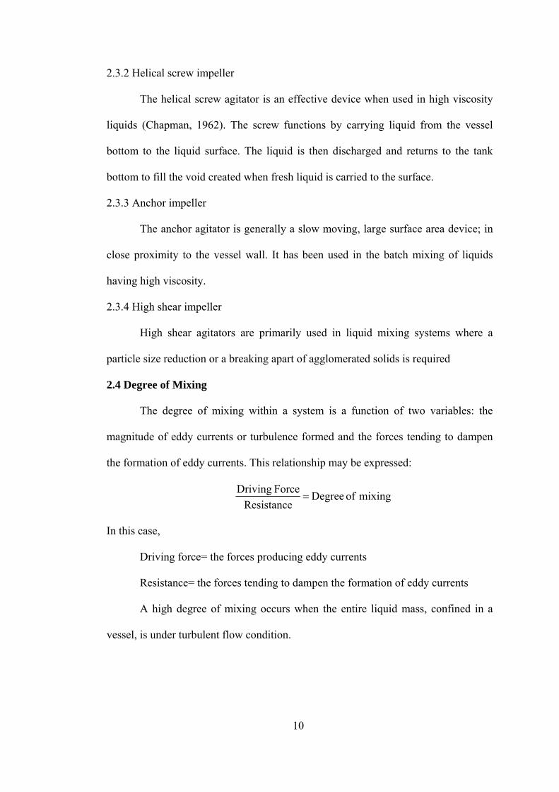
2.4 Degree of Mixing
The degree of mixing within a system is a function of two variables: the
magnitude of eddy currents or turbulence formed and the forces tending to dampen
the formation of eddy currents. This relationship may be expressed:
mixing of Degree Resistance
Force Driving=
In this case,
Driving force= the forces producing eddy currents
Resistance= the forces tending to dampen the formation of eddy currents
A high degree of mixing occurs when the entire liquid mass, confined in a
vessel, is under turbulent flow condition.
10

2.5 Degree of Agitation
Impeller tip speed in m/s is commonly used as a measure of the degree of
agitation in a liquid mixing system. The tip speed of an agitator can be expressed:
ND TS iπ=
Where Di is the diameter of the impeller in m and N is the rotational speed of the
impeller in revolution per second.
2.6 Methods of Measuring Liquid Velocity
The flow characteristics of stirred vessels have been studied by many
investigators using different velocity measuring devices. The first velocity
measurement in a stirred vessel carried out by using the light streak method (Sachs,
1954). Improved version was used by Cutter (1966). Pitot tubes (Nagata, 1955) and
hot wire anemometer (Bowers, 1965) were other types of instruments employed in
the early studies on the measurements of the flow fields in mixing tanks.
None of the above devices are entirely satisfactory. Ideally a measurement
device should not interface with the flow field and should permit the measurement of
instantaneous velocities. Among the non-invasive and instantaneous methods, the
Laser Doppler Velocimetry (LDV) in which velocity is measured using the Doppler
shift of the laser beams crossing the flow field, is the most common method used in
velocity measurements of the complex flows.
LDV was used by Rao and Brodkey (1972), Riet and Soots (1989), Wu and
Petterson (1989), Kresta and Wood (1983). Nevertheless the flow in the stirred
vessel is highly unsteady and time varying large scale motions dominate the flow.
Since the LDV measures velocities on a plane, characterizing the entire flow field
requires long experimental times. In addition LDV cannot be used in opaque media.
11
Therefore Bakker et al. (1996), Ward (1995) were the first to use Particle Image
Velocimetry (PIV) to study the two dimensional flow pattern along the center plane
in the vessel. PIV is quite different from the LDV methods. LDV provides
instantaneous velocity field snapshot in a plane but PIV provides overall flow fields
with spatially resolved eddies but with low temporal resolution.
2.7 Flow Patterns in Stirred Vessel
According to the main directions of the streamlines in the vessel, there are
three principal types of flow. These are tangential flow, radial flow and axial flow.
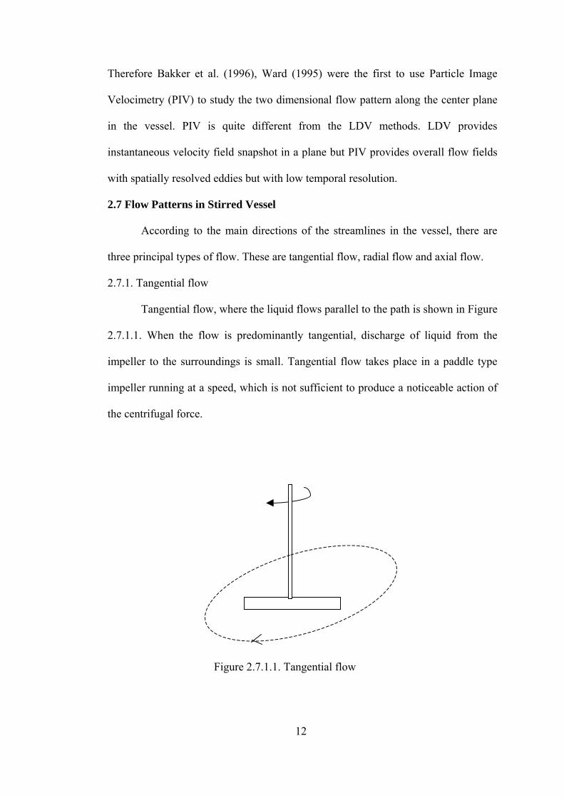
2.7.1. Tangential flow
Tangential flow, where the liquid flows parallel to the path is shown in Figure
2.7.1.1. When the flow is predominantly tangential, discharge of liquid from the
impeller to the surroundings is small. Tangential flow takes place in a paddle type
impeller running at a speed, which is not sufficient to produce a noticeable action of
the centrifugal force.
Figure 2.7.1.1. Tangential flow
12
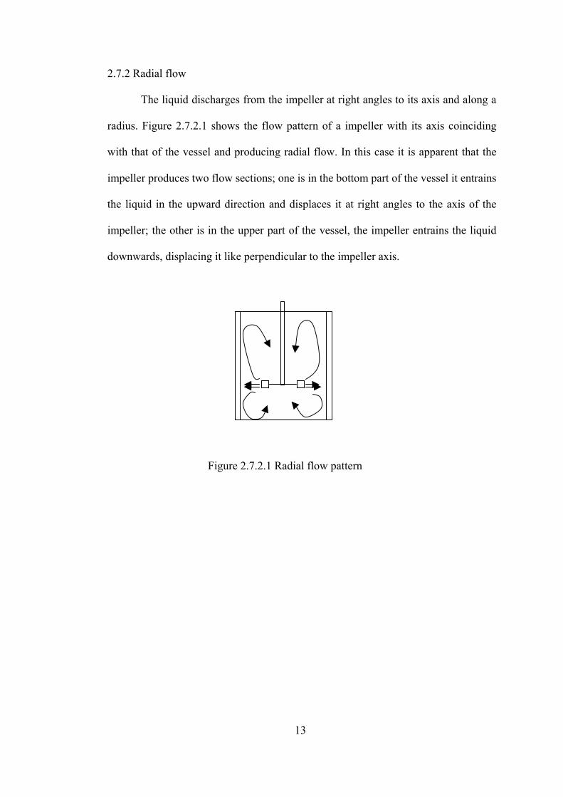
2.7.2 Radial flow
The liquid discharges from the impeller at right angles to its axis and along a
radius. Figure 2.7.2.1 shows the flow pattern of a impeller with its axis coinciding
with that of the vessel and producing radial flow. In this case it is apparent that the
impeller produces two flow sections; one is in the bottom part of the vessel it entrains
the liquid in the upward direction and displaces it at right angles to the axis of the
impeller; the other is in the upper part of the vessel, the impeller entrains the liquid
downwards, displacing it like perpendicular to the impeller axis.
Figure 2.7.2.1 Radial flow pattern
13

2.7.3 Axial flow
Axial flow, in which the liquid enters the impeller and discharges from it
parallel to it axis as shown in Figure 2.7.3.1.
Figure 2.7.3.1. Axial flow pattern
2.8 Flow Model for The Stirred Vessel
One of the most commonly used and extensively studied impeller is the radial
flow Rushton turbine. This is also chosen for this study in order to compare the
results of this study with those of previous studies directly.
In baffled vessels a Rushton turbine impeller develops radial flow pattern.
From the fluid dynamics view point the flow field in an agitated vessel divided into
six following regions (DeSouza and Pike, 1972).
1) The flow from the impeller;
2) Impeller stream impinging on the tank wall;
3) Upper and lower corners of the tank;
4) Flow at the top and bottom of the thank axis;
5) Flow at the center of the tank axis;
6) Two doughnut shaped regions.
14

The most important among them is the impeller region where tank content
and the impeller interacts directly and the required energy to drive the flow is
transferred to the fluid. Due to the high shear rates and sudden accelerations
associated with this region, capturing the flow characteristics accurately around the
impeller through computational methods is a challenging task.
2.9 Power Consumption in Mixing Vessel
The velocity field in stirred vessels provides the details on how fluid moves
inside the tank, no specific information of impeller performance are readily available.
In fact, the power drawn by a rotating impeller is crucial for the process and
mechanical design of agitated vessels.
The power consumption in a liquid mixing system is determined by its
impeller rotational speed and by the various physical properties of the mixing liquid.
Rushton, Costich and Everett (1950) used dimensional analysis to derive the
equations
fi
ei
di
cii
bil
aiT
yFr
xp DWDrDqDHDHDDNNCN )/()/()/()/()/()/()()( Re=
(2.9.1) iR
hB NRNB )/()/(
which, gives the dimensionless Power number as a function of the Reynolds
number , Froude number and number of dimensionless shape factors.
Reynold number and Froude number are defined as:
pN
ReN FrN
µ
ρNDN i2
Re =
15

gDNN i
Fr
2
=
where Di is the impeller diameter (m), N is the impeller speed (s-1), ρ is density
(kgm-3), µ is the viscosity (Pas), g is the gravitational force (ms-2).
In equation (2.9.1):
C = dimensionless constant
= impeller diameter iD
= tank diameter TD
= liquid height lH
= impeller height from bottom of the tank iH
= impeller blade with q
r = impeller blade length
= baffle length W
= reference number for baffles BN
= reference number for impellers RN
BN and determined by convenient choice. For example, in the case of standard
configuration, which is discussed in Chapter 4 is used as a reference, = 4 and
= 6. If these shape factors remain fixed, equation 2.9.1 simplifies to
RN
BN
RN
yFr
xp NNCN )()( Re= (2.9.2)
where C is the over all shape factor which represents the geometry of the system.
Since Froude number links gravitational forces and centrifugal inertial forces, then
16
fully baffled vessel in which no central vortex could form. Therefore the exponent y
of the Froude number is zero, =1 and equation 2.9.2 becomes yFrN )(
xp NCN )( Re= (2.9.3)
Power number, which is dimensionless number relating the resistance force to
the inertia force is expressed as
53N ip D
PNρ
= (2.9.4)
where P is the power in Watt, ρ is the density in , N is the rotational
speed of the impeller in rev/sec and is the impeller diameter.
3/ mkg
iD
2.9.1 Power curves
A plot of versus on log-log coordinates is commonly called a power
curve. The power curve firstly was plotted by Holland and Chapman (1966) for the
standard tank configuration. At low Reynolds number
pN ReN
)10( Re <N , Np decreases
linearly with increasing Re. In this region equation (2.9.3) may be written as
Re101010 logloglog NxCN p += (2.9.5)
The slope x in the viscous region is equal to -1. Therefore for the viscous region,
equation (2.9.5) can be simplified,
12i
53 )/ND ()N ( −= µρρ CDP i (2.9.6)
which can be rearranged to
))(( 32iDNCP µ= (2.9.7)
17

Equation (2.9.7) shows power to be directly proportional to viscosity at any impeller
speed.
When the Reynolds number increases, flow changes from viscous to
turbulent. The power and flow characteristics remain dependent only on the
Reynolds number until 300Re ≅N . At this point enough energy is being transferred
to the liquid enabling vortex formation. The baffles effectively suppress vortexing
and the flow remains dependent on the Reynolds number until . When
flow becomes fully turbulent, the power curve becomes horizontal. Here flow is
independent of both the Froude and Reynolds numbers.
10000Re =N
.
18

CHAPTER 3
DISCRETIZATION METHODS IN FLUID DYNAMICS
3.1 Computational Approach Computational fluid dynamics (CFD) is a tool for solving conservation
equations for mass, momentum and energy in flow geometry of interest. Flows and
associated phenomena can be described by partial differential equations, which are in
many cases extremely difficult to solve analytically due to the non-linear inertial
terms. To obtain accurate results the domain in which the partial differential
equations are described, have to be discretized using sufficiently small grids.
Therefore accuracy of numerical solution is dependent on the quality of
dicretizations used (Ferziger, Peric, 1996).
3.2 Components of the Numerical Simulations
3.2.1 Mathematical model
The starting point of a numerical method is the mathematical model, which is
the selection of the governing equations and initial and boundary conditions.
3.2.2 Discretization of the governing equations
After selection the governing equations, one has to choose suitable
discretization method. There are many approaches, the most important are: finite
difference (FD), finite volume (FV) and finite element (FE) methods. Each of these
methods is used to transform differential equations to the algebraic equations.
19

3.2.3 Generation of computational grid
The discrete locations form numerical grid, which can also be considered as
discrete representation of the solution domain. The numerical grid divides the
solution domain into finite number of subdomains (elements, control volumes).
3.2.3.1 Structured grid
Structured grids consist of families of grid lines with the property that
members of a single family do not cross each other and cross each member of the
other families only once. This allows the lines of a given set to be numbered
consecutively. The disadvantage of structured grid is that they can be used only for
geometrically simple solution domains and another is that it may be difficult to
obtain suitable grid distributions for complicated flow fields.
3.2.3.2 Unstructured grid
For very complex geometries, the most flexible type of grid is one, which can
fit an arbitrary solution domain boundary. In principle, such grids could be used with
any discretization scheme, but they are best adapted finite volume and finite element
approaches. The elements or control volumes may have any shape and there is no
restriction on the number of neighbor elements or nodes. Disadvantage of the
unstructured system of algebraic equation is difficult to solve.
3.2.3.3 Block structured grid
In a block structured grid, there are two or more level subdivision of domain.
There are blocks, which are relatively large segments of the domain; their structure
may be irregular and they may or may not overlap. This kind of grid is more flexible
then the structured grids, since it allows use of finer grids in regions where greater
20

spatial resolutions are required. The main advantage of the block structured grid is
that complex geometries can be handled easily.
3.2.4 Finite approximation
After the choice of grid type, one has to select the approximations to be used
in the discretization process. In the finite difference method, approximations for the
derivatives at the grid points have to be selected. In the finite volume method,
however, one has to select the methods of approximating surface and volume
method. In the finite element method, one has to choose the functions (elements) and
weight functions. The choice influences the accuracy of the approximation, also
affects the difficulty of developing the solution method and speed of the code. More
accurate approximations involve more nodes and result algebraic equations with
dense matrices.
3.2.5 Solution method
Discretization yields a large system of non-linear algebraic equations. The
method of solution depends on the problem. For example for unsteady flows,
methods employed in the solution of the initial value problems are used. The solution
methods of solving algebraic systems can be classified as follows:
1) Direct methods
Direct methods are based on finite number of arithmetic operations leading to
the exact solution of linear algebraic system. Some of these are Gauss elimination,
tridiagonal system and LU decomposition.
21

2) Iterative methods
Iterative methods are based on a succession of approximate solutions, leading
to the exact solution after infinite number of step. A large number of iterative
methods are available. Some of these are Jacobi method, Gauss-Seidel method,
successive over relaxation (SOR), strongly implicit procedure (SIP) and
alternating direction implicit (ADI) method.
3.2.6 Convergence criteria
Finally, one needs to set the convergence criteria for the iterative method due
to decide when to stop iterative process. Usually, there are two levels of iterations,
within which the linear equations are solved and outer iteration that deals with the
non-linearity and coupling of the equations. Deciding when to stop the iterative
process on each level is important from both the accuracy and efficiency point of
views.
3.3 Finite Volume Method
Finite volume method uses the integral form of the conservation equations,
which are discretized directly in the physical space. Solution domain is divided into
a finite number of small control volumes (CVs) by a grid, in contrast to the finite
differences (FD) method, defines the control volumes boundaries. In the finite
volume method two approaches are described. In the usual approach, the solution
domain is discretized and a computational node is assigned to the each control
volume center. However, in the second approach nodel locations are defined first and
constructed CVs around them, so that control volume is faced lie midway between
nodes which boundary conditions are applied as shown in Figure 3.3.1 (J.H. Ferziger
and M.Peric, 1996).
22
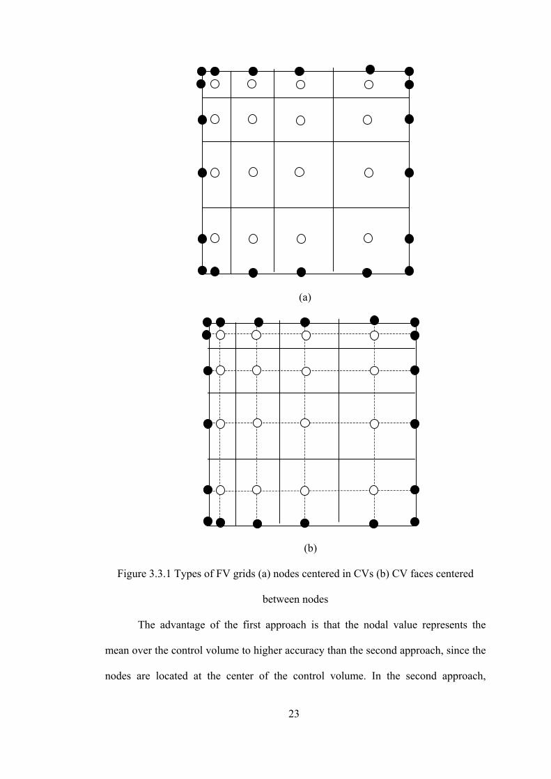
(a)
(b)
Figure 3.3.1 Types of FV grids (a) nodes centered in CVs (b) CV faces centered
between nodes
The advantage of the first approach is that the nodal value represents the
mean over the control volume to higher accuracy than the second approach, since the
nodes are located at the center of the control volume. In the second approach,
23

however, central differences scheme (CDS) approximations of derivatives at control
volume faces are more accurate when the face is midway between two nodes. The
discretization principles are the same for the both approaches.
3.3.1 Discretization process
In this study, discretization of the flow equations within the FASTEST3D,
which is introduced in Chapter 4 in detail was carried out using finite volume
method.
The equations describing fluid flow are derived from the conservation of
mass and momentum. General form of the conservation equations are (Versteeg,
Malalasekera, 1995)
continuity: ( ) 0=+∂∂ vdiv
tρ
ρ (3.3.1)
momentum: ( ) vsTvvdivvt
=−+∂∂ )(ρρ (3.3.2)
where ρ is density, v is velocity, T is the diffusion flux vector, Equation (3.3.2) is
written in terms of a velocity component , obtain iU
( ) uiiii stUvdivUt
=−+∂∂ )(ρρ (3.3.3)
where it is the momentum diffusion and is the source term which represent the
external forces;
uis
jiji it τ= (3.3.4)
iui yPs
∂∂
−= , ghpP ρ+= (3.3.5)
24

The index ‘i’ denotes the direction of the Cartesian coordinate. are the
Cartesian velocity components,
iU
p is the pressure, g is the gravity constant and h the
distance from a given reference level. ijτ are the anisotropic parts of the stress tensor.
For a Newtonian fluid and incompressible laminar flow it can be expressed as the
product of the dynamic viscosity and the rate of strain as:
⎟⎟⎠
⎞⎜⎜⎝
⎛∂∂
+∂∂
=i
j
ji
ij yU
yUµτ (3.3.6)
Figure 3.2 shows the Cartesian coordinate system ( )21 , yy with base vector 1i and
2i and a typical control volume. Equation (3.3.1) and (3.3.2) are to be integrated over
a finite number a control volumes and over the time interval ( )ll tt ,1− .
Here, Divergence theorem is used, which transforms the volume integral of a
vector divergence in to a surface integral:
AdfdVfdivAv∫∫ ≡ (3.3.7)
V is the volume of the control volume and A is the area of its surface, Ad being the
outward directed surface vector normal to this surface. The right hand side of the
equation (3.3.7) represents the net flux of the transport quantity through the control
volume surface. It must be equal to the net source given by the right hand side of
equations (3.3.1) and (3.3.2). In the case of the continuity equation, there is no source
term, i.e. mass is conserved, so the net mass flux must be zero. For the momentum
equations the right hand side ( )uis represents the external forces.
The surface integrals are evaluated on each control volume face and then
summed up. For a two dimensional case the third dimension is unity, and the fluxes
25
in this direction are zero. Since the third dimension is unity the cell face areas are
equal to the length of the line segments connecting the two vertices.
The fluxes are by definition equation (3.3.7) taken positive when directed
outwards. Outward flux through the ‘e’ or east cell face (Figure 3.3.2), , is the
inward flux through the ‘w’ or west cell face of the neighbor control volume can be
expressed as : ( ) . Therefore only two fluxes per control volume need
to be calculated, namely and . The general form of the discretized equation
then becomes:
eI
( )EwPe II −=
eI nI
SIIII snwe =+++ (3.3.8)
where the I’s represent the fluxes through respective cell surfaces. Similarly
subscripts n and s denotes the quantities in the north and south directions as shown in
the Figure 3.3.2.
26

nw
ne
se
sw
w
eP
N
E
s
n
wA
sA
eA
nAy
x
ji =2
ii =1
Figure 3.3.2. A typical control volume and the notation used for a Cartesian 2D grid
eeAe
e AfAdfI .. ≈= ∫ (3.3.9)
The surface vectors on the cell faces are defined as:
( ) ( ) jxxiyyA esnesne −−−= (3.3.10)
( ) ( ) jxxiyyA newnewn −−−= (3.3.11)
where x’s and y’s stand for the horizontal and vertical positions of the cross-sectional
points of the surfaces, respectively. In the case of the continuity equation, the vector
f in equations (3.3.7) and (3.3.9) stands for vρ . The positive, outward directed
fluxes through the east and north cell faces become:
( ) ( ) ( )[ ]esnsneeAe
ee xxVyyUAVAdVFI −−−=≈== ∫ ρρρ ..1 (3.3.12)
27

( ) ( ) ( )[ ]nwewennAn
nn yyVxxUAVAdVFI −−−=≈== ∫ ρρρ ..2 (3.3.13)
1F and denote the average mass fluxes in the positive direction of general
coordinate
2F
1x and 2x respectively. U and V are the x and y components of the
velocity, respectively. The continuity equation then becomes
02211 =−+− snwe FFFF (3.3.14)
eU , , and in equations (3.3.12) and (3.3.13) represent the average values
of the Cartesian velocity components at the appropriate cell faces.
eV nU nV
The left hand side of the momentum equations (3.3.3) has two parts:
convection and diffusion. For the convection fluxes CI , f in equations (3.3.7) and
(3.4.9) is substituted by vUρ , yielding:
eeCe UFI 1≈ (3.3.15)
nnCn UFI 2≈ (3.3.16)
In case of the diffusion fluxes DI , the vector f stands in the U equation for 1t− ,
yielding:
eeDe AjiI .)( 1211 ττ +−≈ (3.3.17)
nnDn AjiI .)( 1211 ττ +−≈ (3.3.18)
The stresses 11τ and 12τ contain velocity derivatives with respect to Cartesian
coordinates, these have to be expressed in term of general coordinate iξ , according
to :
28
⎟⎟⎠
⎞⎜⎜⎝
⎛∂∂
∂∂
−∂∂
∂∂
=∂∂
ηξξηUyUy
JxU 1
(3.3.19)
⎟⎟⎠
⎞⎜⎜⎝
⎛∂∂
∂∂
−∂∂
∂∂
=∂∂
ξηηξUxUx
JyU 1
(3.3.20)
where J is the Jacobian of the coordinate transformation ( ) ( )ηξ ,, fyx = defined
by:
ξηηξ ∂∂
∂∂
−∂∂
∂∂
=yxyxJ (3.3.21)
The Jacobian and derivatives of the equations (3.3.19) and (3.3.20) need to be
evaluated at the cell face locations ‘e’ and ‘n’. For the ‘e’ face, the ξ coordinate is
taken to connect the points P and E (from P to E) and η runs along the ‘e’ cell face
(from the ‘se’ to ‘ne’). The derivativesξ∂
∂x,
η∂∂x
can be approximated as:
PE
PE
e
xxxξξξ −
−≈⎟⎟
⎠
⎞⎜⎜⎝
⎛∂∂
; sene
sene
e
xxxηηη −
−≈⎟⎟
⎠
⎞⎜⎜⎝
⎛∂∂
(3.3.22)
For the simplicity, PE ξξ − is taken which is the distance between point P and
E; analogously,
EPl ,
sene ηη − is set equal to the , the length of the cell face between
vertices ‘ne’ and ‘se’. The Jacobian can then approximated by:
senel ,
( )( ) ( ) ([ ]PEesnesnPEseneEP
e yyxxyyxxll
J −−−−−≈,,
1 ) (3.3.23)
The derivatives in equations (3.3.19) and (3.3.20) can be expressed via expression
equations (3.3.22) and (3.3.23) to yield:
( ) ( ) ( )( )( ) ( ) ( )( )esnPEPEesn
esnPEPEesn
e xxyyxxyyUUyyUUyy
xU
−−−−−−−−−−
≈⎟⎠⎞
⎜⎝⎛
∂∂
(3.3.24)
29
( ) ( ) ( )( )( ) ( ) ( )( )esnPEPEesn
esnPEPEesn
e xxyyxxyyxxUUxxUU
yU
−−−−−−−−−−
≈⎟⎟⎠
⎞⎜⎜⎝
⎛∂∂
(3.3.25)
When the expression (3.3.6) for ijτ are introduced in equations (3.3.17-18) and
relations of the form (3.3.24-25) are used the following expression can be written as
for the diffusion fluxes and : DeI D
nI
( ){ ( ) ( )[ ]( ) ( )( ) ( )( )[ ]( )( ) ( ) ( )[ ]( ) }esnPEesnesnPE
esnPEesnPEesn
esnesnPEe
eDe
xxyyVVyyVVxxxxyyyyUU
xxyyUUV
I
−−−−−−
−−−+−−−
−−+−−−≈
2
2 22
δµ
(3.3.26)
( ){ ( ) ( )[ ]( ) ( )( ) ( )( )[ ]( )( ) ( ) ( )[ ]( ) }nwePNnwenwePN
nwePNnwePNnwe
nwenwePNn
nDn
xxyyVVyyVVxxxxyyyyUU
xxyyUUV
I
−−−−−−
−−−+−−−
−−+−−−≈
2
2 22
δµ
(3.3.27)
It should be noted that the outward diffusion flux thorough the ‘e’ cell face is
the inward flux through the ‘w’ cell face of the neighbor control volume that is
( ) ( )wDeP
Dw II −= and ( ) ( )S
DnP
Ds II −= ; also nV δ and eV δ are defined as the
scalar product of the surface vector nA and eA respectively.
( ) ( ) ( ) ( )PNnwePNnwenn yyxxxxyyPNAV −−+−−−== . δ (3.3.28)
( ) ( ) ( ) ( )PEnsnPEesnee yyxxxxyyPEAV −−+−−−== . δ (3.3.29)
For the V -momentum equation, the convection and diffusion fluxes are
obtained as:
30

eeCe VFI 1≈ (3.3.30)
nnCe VFI 2≈ (3.3.31)
and
( ){ ( ) ( )[ ]( ) ( )( ) ( )( )[ ]( ) ( ) ( ) ( )[ ]( ) }esnesnPEPEesn
esnPEesnPEesn
esnesnPEe
eDe
yyxxUUxxUUyyyyxxxxVV
xxyyVVV
I
−−−−−−
−−−+−−−
−−+−−−≈
2
2 22
δµ
(3.3.32)
( ){ ( ) ( )[ ]( ) ( )( ) ( )( )[ ]( ) ( ) ( ) ( )[ ]( ) }nwewePNPNnwe
nwePNnwePNnwe
nwenwePNn
nDn
yyxxUUxxUUyyyyxxxxVV
yyxxVVV
I
−−−−−−
−−−+−−−
−−+−−−≈
2
2 22
δµ
(3.3.33)
The source term in the momentum equations are integrated over the control volume;
( ) VsdVsSV
Puu δ∫ ≈= (3.3.34)
Thus, the gradients xP
∂∂
and yP
∂∂
need to be evaluated at point P by analogy
to equations (3.4.19-20-21) and (3.4.23), these gradients are calculated as:
( )( ) ( )( )( )( ) ( )( )wesnsnwe
wesnsnwe
P yyxxyyxxyyPPyyPP
xP
−−−−−−−−−−
≈⎟⎠⎞
⎜⎝⎛
∂∂
(3.3.35)
( )( ) ( )( )( )( ) ( )( )wesnsnwe
snwewesn
P yyxxyyxxxxPPxxPP
yP
−−−−−−−−−−
≈⎟⎟⎠
⎞⎜⎜⎝
⎛∂∂
(3.3.36)
Source terms for the momentum equations can be approximated as:
( )( ) ( )( )wesnsnwep
u yyPPyyPPS −−+−−−≈ (3.3.37)
( )( ) ( )( )snwewesnp
v xxPPxxPPS −−+−−−≈ (3.3.38)
31
When all the flux components and the discretized sources are introduced in equation
(3.4.8), an algebraic counterpart of the differential equation is obtained.
[ ]{ } { }SA =φ (3.3.39)
where is the [ ]A MM × matrix, M is the total number of the control volumes, { }φ
is the dependent variable vector of M nodal values and { }S is similar vector
containing source terms.
3.4 Solution Methods
The previous discussion showed the partial differential equations may be
discretized using FV method. The result of the discretization process is a system of
algebraic equations, which are linear or nonlinear according to the nature of partial
differential equations from which they are derived.
Two methods are available for the solution of linear algebraic equations: the
direct and iterative methods. In non-linear case, the discretized equations must be
solved by using iterative technique.
3.4.1 Direct methods
Direct methods are based on a finite number of arithmetic operations leading
to the exact solution of a linear algebraic system in one step.
3.4.1.1 Gauss elimination
The basic method for solving linear systems of algebraic equations is Gauss
elimination. Its basis is the systematic reduction of large systems of equations to
smaller ones (Heath, 1997).
32

(3.4.1)
⎟⎟⎟⎟⎟
⎠
⎞
⎜⎜⎜⎜⎜
⎝
⎛
=
nnnnn
n
n
aaaa
aaaaaaaa
A
L
MOMMM
K
K
321
2232222
1131211
The base of the algorithm is the technique for eliminating below the diagonal matrix
element that is replacing it with zero. After this operation, the original matrix is
replaced by the upper triangular matrix:
⎟⎟⎟⎟⎟
⎠
⎞
⎜⎜⎜⎜⎜
⎝
⎛
=
nn
n
n
a
aaaaaaa
U
L
MOMMM
K
K
000
0 22322
1131211
(3.4.2)
After this step all of the elements except in the first row differ from in the original
matrix A . Triangular linear systems are solved by successive substitution process,
which is called back-substitution.
3.4.1.2 Tridiagonal systems
A finite difference approximation provides an algebraic equation at each grid
node. Each equations contains only the variable at its own node and its left and right
neighbors as shown in Figure 3.4.1.2.1.
P EW
i1−i 1+i
Figure 3.4.1.2.1. 1 D Cartesian grid for FD methods
iiiEi
iPi
iW QAAA =++ +− 11 φφφ (3.4.3)
33

The corresponding matrix A has non zero terms only on its main diagonal
and the diagonal above and below it. Such matrix is called tridioganal shown Figure
3.4.1.2.2.
⎥⎥⎥⎥
⎦
⎤
⎢⎢⎢⎢
⎣
⎡
00
Figure 3.4.1.2.2. Schematic representation of the tridioganal matrix
Gauss elimination is preferred for solving tridioganal systems since only one
element needs to be eliminated from each row during the forward elimination
process.
3.4.2 Iterative methods
The basis of iterative methods is to perform a small number of operations on
the matrix element of the algebraic system, the aim of approach in the exact solution
within a preset level of accuracy and small number of iteration. A large number of
iterative methods are available some of these are:
1) Jacobi method
2) Gauss-Seidel method
3) Successive over relaxation (SOR) method
4) Alternating direction implicit (ADI) method
5) Strongly implicit procedure (SIP)
6) Conjugate gradient method
7) Multi grid method
34
3.4.3 Solution of the non-linear equations
There are two types techniques for solving non linear equations: Newton-like
and global. Newton-like techniques are much faster when a good estimate of solution
is available but global techniques ensure the solution to converge.
3.5 Convergence Criteria
When using iterative solvers, it is important to know when to stop. The most
common procedure is based on the difference between two successive iterates; the
procedure is stopped when this differences, measured by some norm, is less that pre
selected value.
The numerical solution should approach the exact solution niu ),( txu of the
differential equations at any points xixi ∆= and time tntn ∆= when x∆ and t∆
tend to zero, that is, when the mesh is refined and being fixed. This condition
implies that and goes to infinity while
ix nt
i n x∆ and t∆ goes to zero (C. Hirssch,
1997). This condition for convergence of the numerical solution to the exact solution
of the differential equation express that the error,
) ,( nnxiuuni
ni ∆∆−=ε
satisfies the following convergence condition;
0lim00 =
→∆→∆
ni
xt ε at fixed values of xixi ∆= and tntn ∆= .
3.6 Numerical Methods in Our Study
Numerical techniques described above are all of the methods which can be
used for solution of any mathematical model based on computational fluid dynamics.
In our study for the discretization of the incompressible Navier-Stokes equations in
35

time and space, finite volume method was used and block structured grid was
selected because of the easy treatment of the complex geometry. At the end of the
discretization process, linear algebraic equation was obtained and this matrix
equation solved by using strongly implicit SIP method of Stone time integration by
second order Crank-Nicolson scheme. The inherently time-dependent geometry of
stirred vessel is simulated by a multiple frame of reference approach which is
mentioned in Chapter 4.
Besides of these numerical techniques, for the treatment of the rotating
impeller in mixing tank some new methods have been introduced. Detailed
information is given in the following parts.
3.7 Numerical Methods Used In Mixing Applications
Improvements in computer hardware and capacity of the memory resulting in
developed of predictive methods based on computational fluid dynamics (CFD) and
capable of providing detailed information not only flow and turbulence field but also
impeller performance characteristics like impeller power number and pumping
number in the stirred tank.
In the past most of the studies for the flow simulations in the stirred tanks are
based on steady-state analyses (Harvey and Greaves, 1982), (Ranade and Joshi,
1989), (Bakker, 1992). Most of these investigators have treated the rotating impeller
as a black box, since this approach requires boundary condition in the immediate
vicinity of the impeller, which must be determined experimentally. Though this
approach was successful in the prediction of the flow characteristics in the bulk of
the tank, but it was restricted to the conditions for which input data are available are
36
not for true predictions. Since a single set of impeller boundary conditions must be
used for geometrically similar systems, it cannot be used large number alternative
mixer configurations
To overcome limitations associated with the requirement of the experimental
impeller boundary conditions, recently some methods have been developed. These
methods are namely momentum source, snapshot, sliding mesh and multiple frame of
reference method which was used in this study.
3.7.1 Impeller models
As mentioned above, there are four different approaches for the modeling of
the impeller. They are analyzed in further detailed below especially focus on clicking
method.
3.7.1.1 Momentum source method
Momentum source model is based on aerofoil aerodynamics. In this model,
the impeller blades are replaced with finite blade section by dividing the blade into a
number of vertical strips from the hub to tip (Xu and McGrath, 1996), (Pericleous
and Patel, 1987). The blade sections inside each strip are approximated to an aerofoil
and aerofoil aerodynamics is applied. No experimental data are required in this
model but it is restrictive since the flow inside the impeller is assumed to have no
azimuthal direction of the flow between the blades.
3.7.1.2 Snapshot method
In the snapshot method, impeller blades are fixed at one particular position
with respect to the baffles. This method can be explained as follows: in a real case
rotation of the blade causes suction of fluid at the back side of the impeller blades
and equivalent ejection of fluid from the front side of the blades. These phenomena
37

of ejection and suction have been modeled by snapshot formulation (Ranade and
Dommeti, 1996). That is, computational cells adjacent to the back side of the blades
are modeled by specifying the mass sources, it can be defined as:
bcbcm WAS ρ−= (3.7.1.2.1)
where and are the area of the surface of the computational cell which is the
adjacent to the impeller blade. For the computational cell on the back side of the
blades are modeled by specifying the mass sinks and it is defined by expression
(3.7.1.2.1) with the positive sign
bcA bcW
bcbcm WAS ρ= (3.7.1.2.2)
3.7.1.3 Sliding mesh method
In the sliding mesh method, the tank is dividing in to two regions that are
impeller region and the tank region. The tank region includes the bulk of the liquid,
the tank wall, the tank bottom and the baffles. The grid in the impeller region rotates
with the impeller while the grid in the tank remains stationary (Bakker et al., 1996),
(Lane and Koh, 1997), (Jaworski et al., 1997), (Lee and Yanneskis, 1996). The two
grids slide past each other at a cylindrical interface. Two regions are implicitly
coupled at the interface via a sliding mesh algorithm which takes in to account the
relative motion between the two sub-domains and performs the conservative
interpolation.
38

CHAPTER 4
NUMERICAL METHOD FOR SOLVING TIME DEPENDENT FLUID DYNAMICS
4.1 Numerical Methods
In this section numerical method and tools used in the flow simulations are
explained. In the past most of the studies for the flow simulations in the stirred tanks
are based on steady-state analyses as outlined in chapter 3. This technique, however,
needs some experimentally obtained boundary conditions in the vicinity of the
impeller. Therefore this method is not practical to study large number of impeller
configuration.
To overcome limitations associated with the requirement of the experimental
impeller boundary conditions, recently some methods have been developed. These
methods are as previously described as momentum source method, snapshot method
and sliding mesh method. Another method being used in the mixing simulations is
multiple frame of reference method, which is the technique employed in this study
due to some shortcomings of the mentioned alternative methods. For example in the
momentum source method the impeller modeling is rather restrictive because the
flow inside the impeller is assumed to have no azimuthal direction variations, so
there is no straight forward simulation of the flow between the blades. The snapshot
technique provides a relatively less computational intensive for the simulation of
flow between impeller blades. Finally, the sliding mesh method is based on the time
dependent laminar flow simulation only. It is also highly CPU time demanding.
39

4.1.1 Multiple frame of reference method
In this study all of the numerical simulations are carried out by using multiple
frame of reference with clicking method within the FASTEST3D code. In this
method tank is divided into two frames. These are rotating frame and stationary
frame. Rotating reference frame encompasses the impeller and the flow surrounding
it and stationary frame includes the tank, the baffles and the flow outside the impeller
frame. Figure 4.1.1.1 depicts the configuration used. This figure shows that the tank
is formed by twenty three blocks, seventeen blocks of them are defined as rotating
which are represented by the red color blocks and remaining are six stationary
blocks, which are indicated by yellow color. Interface blocks are not physically
defined by the user when the grid generation is being constructed. These blocks are
defined by the program as an imaginary section to provide the interaction between
the rotating and stationary blocks. The interface blocks are represented by dark blue
and light blue as shown in Figure 4.1.1.2. Numbers of the control volumes which are
forming the interface blocks belonging to stationary and rotating parts are equal at θ
direction. In the stationary blocks, governing equations are the common equation of
continuity and Navier Stokes equations. In the flow region surrounding the impeller
those governing equations are modified for the rotating frame.
40

Figure 4.1.1.1 Rotating and stationary blocks in the solution domain
Figure 4.1.1.2 Interface sections of the stationary and rotating blocks
41
In this method clicking step size and number of the time step have to be defined by
user before executing the program. Once the flow quantities such as velocities and
pressures are determined for a certain control volume near the impeller, for the next
time step those quantities are transferred as initial condition to the other control
volume which is in front of the original control volume by the clicking step size in
the rotation direction. Therefore, by this procedure rotation around the impeller is
mimicked. Once the clicking step size and angular velocity are set by the user, time
step is calculated according to those values by the code.
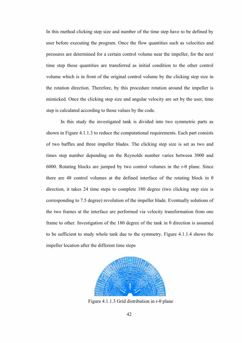
In this study the investigated tank is divided into two symmetric parts as
shown in Figure 4.1.1.3 to reduce the computational requirements. Each part consists
of two baffles and three impeller blades. The clicking step size is set as two and
times step number depending on the Reynolds number varies between 3000 and
6000. Rotating blocks are jumped by two control volumes in the r-θ plane. Since
there are 48 control volumes at the defined interface of the rotating block in θ
direction, it takes 24 time steps to complete 180 degree (two clicking step size is
corresponding to 7.5 degree) revolution of the impeller blade. Eventually solutions of
the two frames at the interface are performed via velocity transformation from one
frame to other. Investigation of the 180 degree of the tank in θ direction is assumed
to be sufficient to study whole tank due to the symmetry. Figure 4.1.1.4 shows the
impeller location after the different time steps
Figure 4.1.1.3 Grid distribution in r-θ plane
42
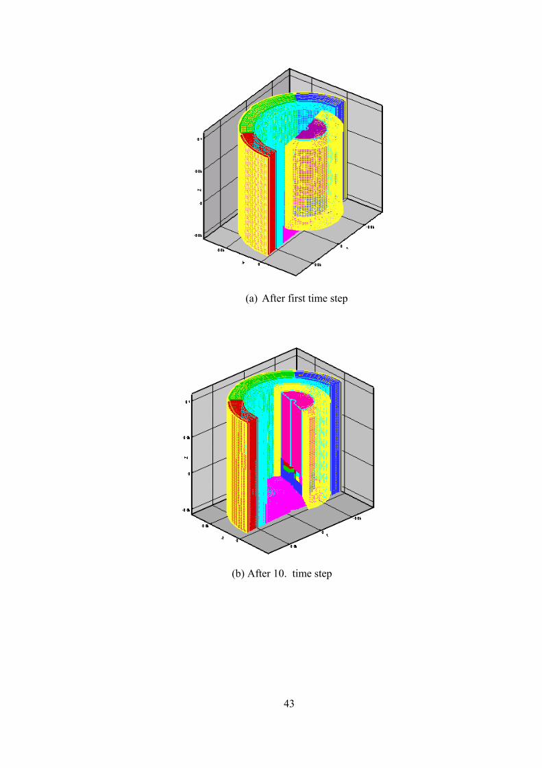
(a) After first time step
(b) After 10. time step
43
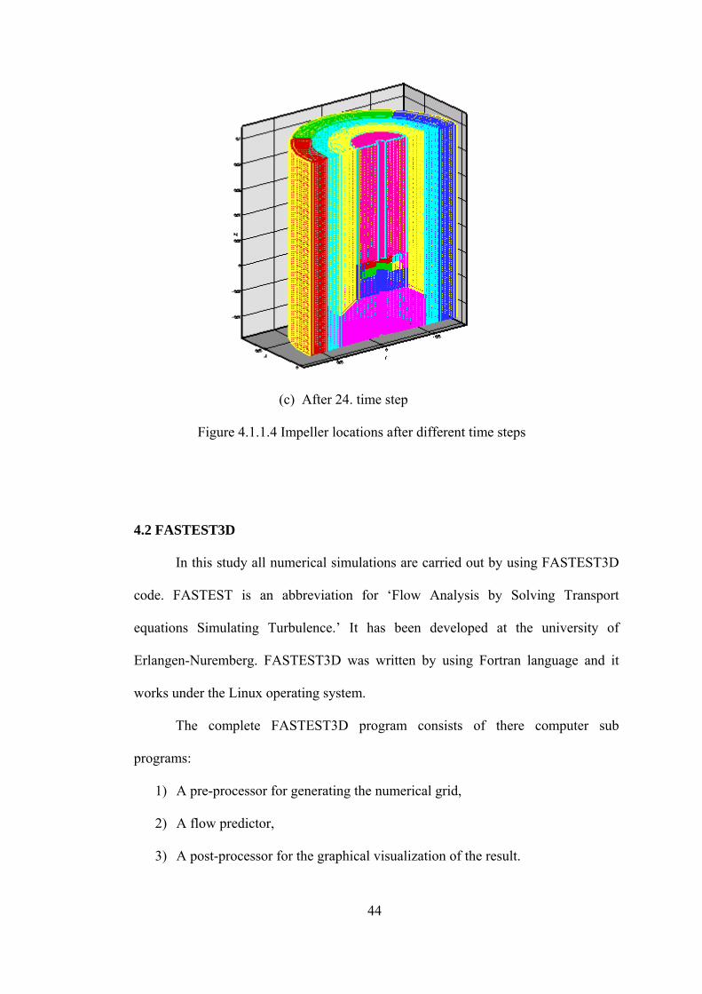
(c) After 24. time step
Figure 4.1.1.4 Impeller locations after different time steps
4.2 FASTEST3D
In this study all numerical simulations are carried out by using FASTEST3D
code. FASTEST is an abbreviation for ‘Flow Analysis by Solving Transport
equations Simulating Turbulence.’ It has been developed at the university of
Erlangen-Nuremberg. FASTEST3D was written by using Fortran language and it
works under the Linux operating system.
The complete FASTEST3D program consists of there computer sub
programs:
1) A pre-processor for generating the numerical grid,
2) A flow predictor,
3) A post-processor for the graphical visualization of the result.
44

A typical FASTEST3D operation can be summarized as follows: Firstly a grid is
generated by taking into account the shape and size of the tank and impeller. Details
of this process are being explained under the topic of the grid generation and
parameters. Other parameters such as angular velocity, fluid properties, clicking step
size and time step number are also supplied to the code. The code then solves the
mixing problem and produces quantities characterizing the flow field in the tank such
as velocity components, turbulence and pressure quantities and power consumption
as shown in Figure 4.2.1.
FASTEST3Dgeneration grid
elocityimpeller vproperties fluid
size step clickingsize step time
input
componentsvelocity field pressure
quantities turbulence
output
power number
Figure 4.2.1 Flow chart of the running FASTEST
FASTEST3D is a flexible code that can be modified according to the specific fluid
flow problems. Its major drawback is that it is not user friendly and to master the
code one needs a lot of practice and trial-error
4.3 Grid generation
For the treatment of complex geometries like mixing tank, block structured
irregular grid is used in FASTEST3D. These globally unstructured, but locally
structured grids can be viewed as a compromise between the flexibility of fully
unstructured grids and numerical efficiency of globally structured grids. Figure 4.3.1
shows a block structured grid which is used in this study. Solution domain is divided
45

into symmetric parts. Each one encompassing two baffles and three impeller blades
(Figure 4.3.2). Our solution domain consists of 23 blocks and total number of
computational cells used is 248020. Table 4.3.1 shows number of control volume in
the blocks-.
Table 4.3.1 Number of the control volumes in the blocks
Block number θ r z Number of control volumes
Block 1: 7× 5× 5= 175 CVs
Block 2: 7× 5× 5= 175 CVs
Block 3: 7× 5× 12= 420 CVs
Block 4: 14× 5× 5= 350 CVs
Block 5: 14× 5× 5= 350 CVs
Block 6: 14× 5× 12= 840 CVs
Block 7: 14× 5× 5= 350 CVs
Block 8: 14× 5× 5= 350 CVs
Block 9: 14× 5× 12= 840 CVs
Block 10: 7× 5× 5= 175 CVs
Block 11: 7× 5× 5= 175 CVs
Block 12: 7× 5× 12= 420 CVs
Block 13: 48× 5× 5= 1200 CVs
Block 14: 48× 5× 5= 1200 CVs
Block 15: 48× 17× 10= 8160 CVs
Block 16: 48× 17× 52= 42432 CVs
Block 17: 48× 15× 74= 52380 CVs
Block 18: 48× 32× 20= 30720 CVs
46

Table 4.3.1 Number of the control volumes in the blocks continued.
Block number θ r z Number of control volumes
Block 19: 12× 10× 94= 11280 CVs
Block 20: 23× 10× 94= 21620 CVs
Block 21: 11× 10× 94= 10340 CVs
Block 22: 48× 12× 94= 54144 CVs
Block 23: 48× 2× 94= + 9024 CVs
Total 248020 CVs
Figure 4.3.1 Block structured irregular grid.
47
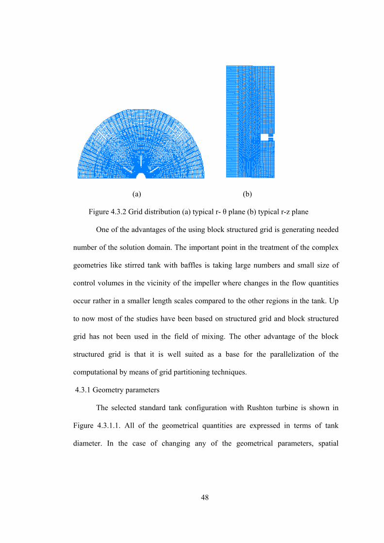
(a) (b)
Figure 4.3.2 Grid distribution (a) typical r- θ plane (b) typical r-z plane
One of the advantages of the using block structured grid is generating needed
number of the solution domain. The important point in the treatment of the complex
geometries like stirred tank with baffles is taking large numbers and small size of
control volumes in the vicinity of the impeller where changes in the flow quantities
occur rather in a smaller length scales compared to the other regions in the tank. Up
to now most of the studies have been based on structured grid and block structured
grid has not been used in the field of mixing. The other advantage of the block
structured grid is that it is well suited as a base for the parallelization of the
computational by means of grid partitioning techniques.
4.3.1 Geometry parameters
The selected standard tank configuration with Rushton turbine is shown in
Figure 4.3.1.1. All of the geometrical quantities are expressed in terms of tank
diameter. In the case of changing any of the geometrical parameters, spatial
48
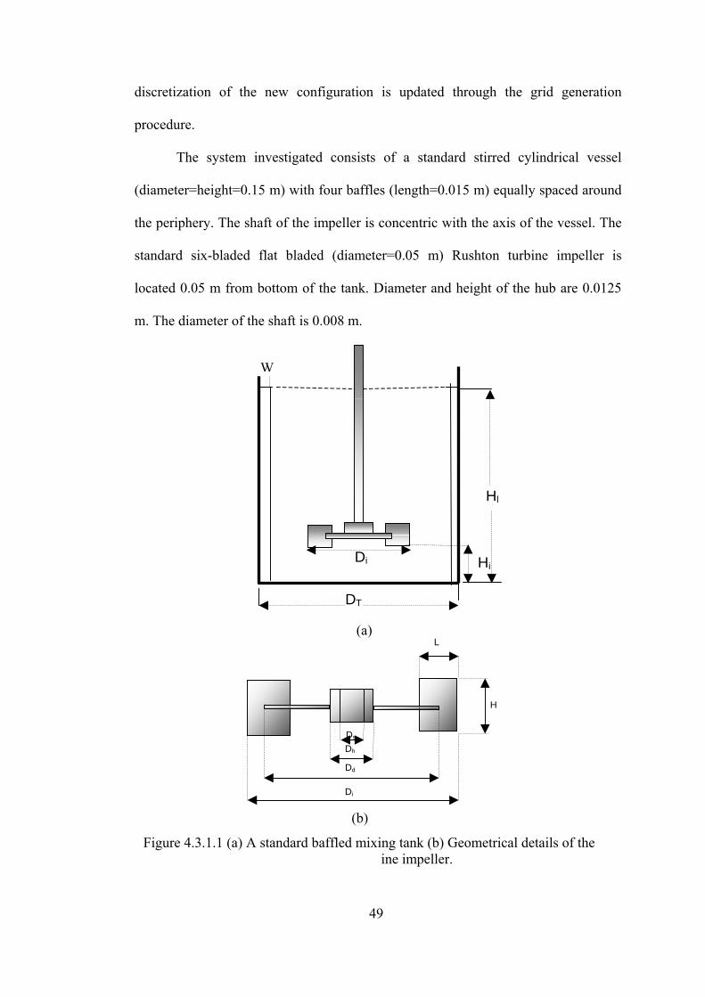
discretization of the new configuration is updated through the grid generation
procedure.
The system investigated consists of a standard stirred cylindrical vessel
(diameter=height=0.15 m) with four baffles (length=0.015 m) equally spaced around
the periphery. The shaft of the impeller is concentric with the axis of the vessel. The
standard six-bladed flat bladed (diameter=0.05 m) Rushton turbine impeller is
located 0.05 m from bottom of the tank. Diameter and height of the hub are 0.0125
m. The diameter of the shaft is 0.008 m.
Ruhton disk turb
Di
Dd
L
Dh
Ds
H
DT
Hi
Hl
Di
W
(b)
(a)
Figure 4.3.1.1 (a) A standard baffled mixing tank (b) Geometrical details of the ine impeller.
49

In this study, the geometrical parameters shown in Figure 4.3.1.1 are set as follows:
DT= Tank diameter 0.15 m
Di= Impeller diameter; Di =DT/3=0.05 m
Hl= Height of the liquid; Hl= DT=0.15 m
Hi= Impeller height from bottom of the tank; Hi= DT/3=0.05 m
W= Length of the baffles; W=3Di/10=0.015 m
L= Length of the blade; L= Di/4=0.0125 m
H=Height of the blade; H= Di/5=0.01m
Dd= Diameter of the disc; Dd=3Di/4=0.0375 m
Dh= Diameter of the hub; Dh= Di/4=0.0125 m
Ds= Diameter of the shaft; Ds=4Di/25=0.008 m
4.4 Computational requirements
Prior to the simulation, the selected numerical tools that suit best for the
numerical simulation of the stirred tank have to be specified. Details of these tools
and general guidelines to make a suitable selection are covered in chapter 3.
Regarding this process the following steps are taken in process of setting up
numerical scheme:
1) Selection of a discretization method of the equations. This implies selection
between finite difference, finite element or finite volume methods as well as
selection of accuracy of the spatial and, eventually time discretization.
2) Selection of a solution method for the algebraic system of equations which is
obtained from discretization
50
3) Analysis of the selected numerical algorithm. This step concerns the analysis
of the ‘qualities’ of the scheme in terms of stability and convergence
properties.
Concerning the numerical method FASTEST3D to solve the incompressible Navier-
Stokes equations composed of the following components: second order finite volume
discretization in time and space, strongly implicit SIP method of Stone for solving a
large system of linear equations and time integration by second order Crank-
Nicolson scheme. The inherently time-dependent geometry of stirred vessel is
simulated by a multiple frame of reference approach, which is mentioned above.
Space discretization is introduced in Chapter 3 therefore here other features of the
implemented numerical methods are explained.
4.4.1 Time discretization
In addition to the spatial discretization a discretization in time is required to
obtain solution of the unsteady problem. Time may be regarded as an additional
coordinate, therefore a special problem can be considered as sequence of levels at
several times, so-called time levels as shown Figure 4.4.1.1. In contrast to spatial
discretization the variable values have to be determined before moving to the next
time level. New time levels are always extrapolated from the older one.
51
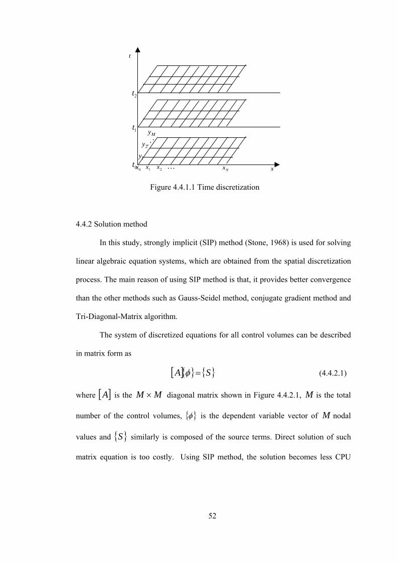
N
L
2y
1y
My
0x 1x 2x Nx x0t
1t
t
2t
Figure 4.4.1.1 Time discretization
4.4.2 Solution method
In this study, strongly implicit (SIP) method (Stone, 1968) is used for solving
linear algebraic equation systems, which are obtained from the spatial discretization
process. The main reason of using SIP method is that, it provides better convergence
than the other methods such as Gauss-Seidel method, conjugate gradient method and
Tri-Diagonal-Matrix algorithm.
The system of discretized equations for all control volumes can be described
in matrix form as
[ ]{ } { }SA =φ (4.4.2.1)
where is the [ ]A MM × diagonal matrix shown in Figure 4.4.2.1, M is the total
number of the control volumes, { }φ is the dependent variable vector of M nodal
values and { similarly is composed of the source terms. Direct solution of such
matrix equation is too costly. Using SIP method, the solution becomes less CPU
}S
52

time demanding. In this method the specified matrices are by separated into upper
and lowers triangular matrices (Figure 4.4.2.2).
The matrix equation then becomes
[ ]{ } [ ][ ]{ } { }SULC == φφ (4.4.2.2)
Therefore the solution becomes easier, since the triangular matrices can be inverted
by simple forward and backward substitution. The triangular matrices [ and ]L [ ]U
have non-zero coefficients only on diagonals which correspond to the non non-zero
diagonals in the matrix The product matrix [ ]A [ ]C has two more diagonals than the
matrix as shown in Figure (4.4.2.2). The coefficients of the matrix [ can be
expressed through the coefficients of the
[ ]A ]C
[ ]L and [ ]U matrices, denoted by b and
analogously to the coefficients a of the matrix [ ]A .
aPaS aN
aW
aE
1
2
2 L NJ
NJ
L IJ LM
M
M
M
IJ
M
.
W φ
S φ
P φ
N φ
E φ
= PS
Figure 4.4.2.1 Schematic presentation of matrix equations (4.4.2.1)
53
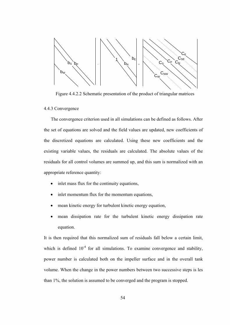
bPbS
bW
1 bN
bE CPCS CN
CW
CE
CNW
. =
Figure 4.4.2.2 Schematic presentation of the product of triangular matrices
CSE
4.4.3 Convergence
The convergence criterion used in all simulations can be defined as follows. After
the set of equations are solved and the field values are updated, new coefficients of
the discretized equations are calculated. Using these new coefficients and the
existing variable values, the residuals are calculated. The absolute values of the
residuals for all control volumes are summed up, and this sum is normalized with an
appropriate reference quantity:
• inlet mass flux for the continuity equations,
• inlet momentum flux for the momentum equations,
• mean kinetic energy for turbulent kinetic energy equation,
• mean dissipation rate for the turbulent kinetic energy dissipation rate
equation.
It is then required that this normalized sum of residuals fall below a certain limit,
which is defined 10-4 for all simulations. To examine convergence and stability,
power number is calculated both on the impeller surface and in the overall tank
volume. When the change in the power numbers between two successive steps is les
than 1%, the solution is assumed to be converged and the program is stopped.
54

In the simulation at Re=10000, a time step size of 0.00521 s is used and up to
3000 time steps were performed, resulting in 62.37 revolutions to achieve the steady
state flow in terms of the turbulent quantities and power number. Calculation time is
approximately 5 hours per impeller revolution on a P III 1Ghz computer.
55

CHAPTER 5
RESULTS AND DISCUSSIONS
As mentioned before agitated vessels are used extensively in industry for
conducting a variety of the processes. One of the most fundamental needs for the
analysis of these processes is the knowledge of flow structure in such vessels. The
flow structures are dependent on the type of agitator and other parameters like
impeller clearance from the bottom of the tank and baffle length. As a result of these
dependencies our investigation has focused on the effects of impeller rotational
speed, N, and baffle length on the flow field and power consumption.
In this study our results consist of two parts: In the first part, we investigate
the flow field generated by Rushton turbine in both laminar and turbulent regimes
using Newtonian silicone oil and water as working fluids in the baffled tank,
respectively. Table 5.1 shows the impeller speed, N (rpm), and corresponding
impeller Reynolds numbers.
Water Silicone oil
ρ= 1000 kg/m3; µ=0.001 Pas ρ=1309 kg/m3; µ=0.0159 Pas
Reynolds number 10000 2069 760 100 20
Impeller speed (rpm) 240 49.6 279 36,76 7,3
Table 5.1. Impeller speed and corresponding Reynolds number
In the second part the effects of the baffle length on the power consumption or power
number at various Reynolds numbers were considered.
56
5.1. Effect of the Reynolds Numbers on the Velocity Field
The flow fields obtained within the Reynolds number range from 10 to 10000
are presented in Figure 5.1.1 in the form of velocity vectors. The figure depicts the
velocities in the half of the vertical cross section cut at the center of the tank. Lengths
of the vectors are proportional to the magnitude of the liquid velocity. At laminar
region which corresponds to Re=10, 20, 100, liquid around the impeller moves with
the impeller rotation smoothly and liquid distant from the impeller is stagnant. In
addition to these, two small vortex rings exist in the flow one below the impeller
plane and the other above the impeller plane. In this region, the resistance to impeller
rotation is mainly due to viscous effects.
Re=760, 2069 correspond to the transition region. In this region the flow
around the impeller becomes unstable and turbulence sets in. Discharge flow notably
increases and reaches a maximum. Now the stagnant zones which are observed in the
laminar region disappear. In this region, the liquid away from the impeller is still
laminar eddies start to form as a result of velocity gradients within the liquid. Also
two vortex centers are observed and they get closer to the impeller plane as impeller
speed is increased. No experimental results have been found in the literature for the
flows in transition region so as to compare the results that were obtained in this
study. Moreover, working numerically in this region is very difficult, since there is
not any applicable turbulent model to the flow field at the corresponding Reynolds
numbers. However, we carried out the simulations using DNS (Direct Solution of
Navier Stokes Equations) method. The results obtained in this region such as velocity
and power number values fit well with those results obtained in laminar and turbulent
regions. Therefore the methods used in this study for the transition region may be
57
considered as satisfactory. Briefly the overall flow pattern in this region is irregular
and flow characteristics are similar to turbulent regime.
At turbulent regime where Reynolds number is larger than 104 the flow
pattern is highly unsteady and the large eddies form at the vicinity of the impeller
plane and secondary small vortices appear in the regions away from the impeller
because of the tank lid. Now stagnant zones and laminar zones, which are observed
in the laminar and transition regions disappear. Discharge flow from the impeller
notably increases and reaches a maximum and generates vertical circulation. As a
result of this phenomena at this region mixing operation becomes highly efficient as
shown in Figure 5.1.1(a). The flow field is not symmetric since the impeller is not
symmetrically located with respect to vertical position. Its location is one third of the
tank diameter from the tank bottom.
Through the simulations the flow field is determined for the entire tank. The
details of the flow characteristics for any given location in the tank are readily
available. In the forthcoming sections, on the other hand, flow field in various
vertical and horizontal cross-sections of the tank is considered only for the sake of
simplicity. Those locations are mainly regions around the impeller, which have the
most important impact on the overall flow field.
58
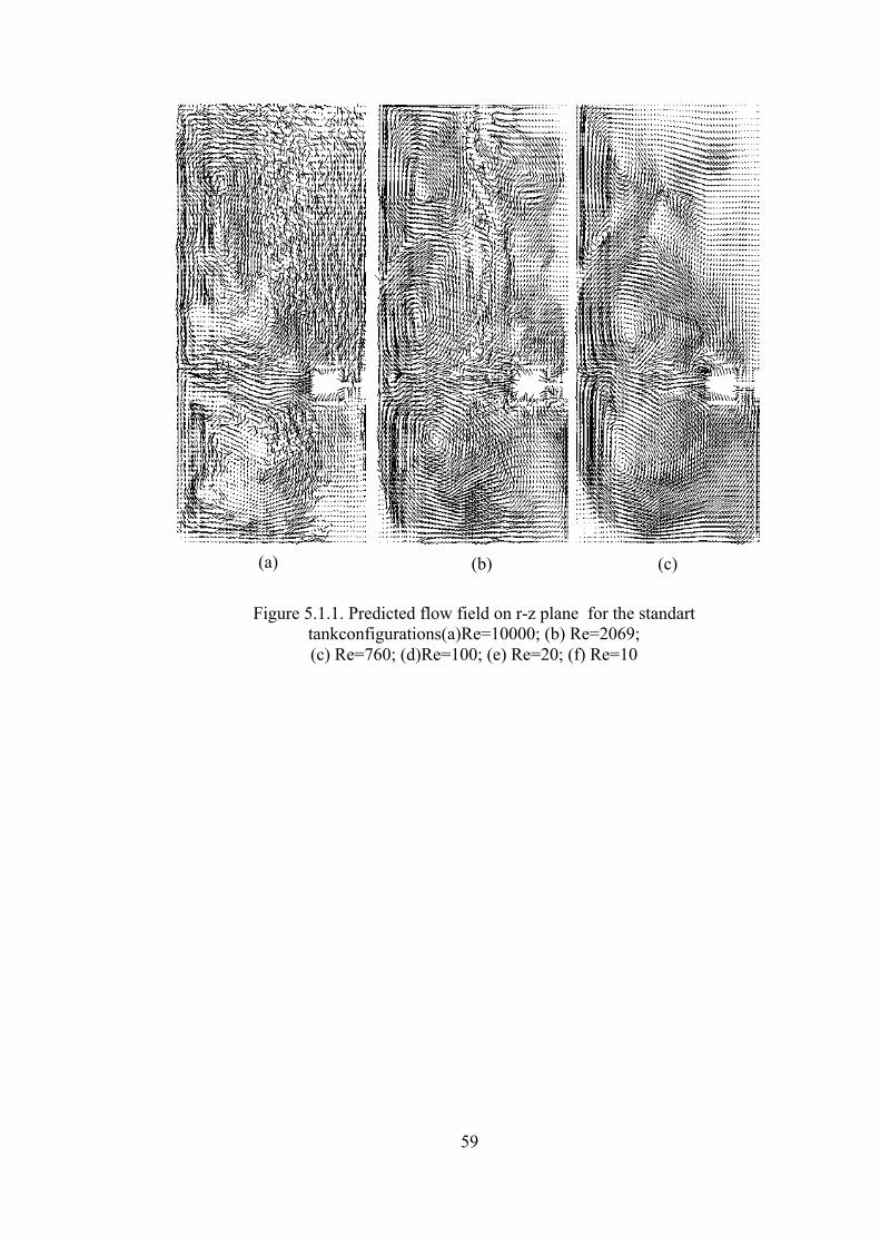
(a) (b) (c)
Figure 5.1.1. Predicted flow field on r-z plane for the standart
tankconfigurations(a)Re=10000; (b) Re=2069; (c) Re=760; (d)Re=100; (e) Re=20; (f) Re=10
59
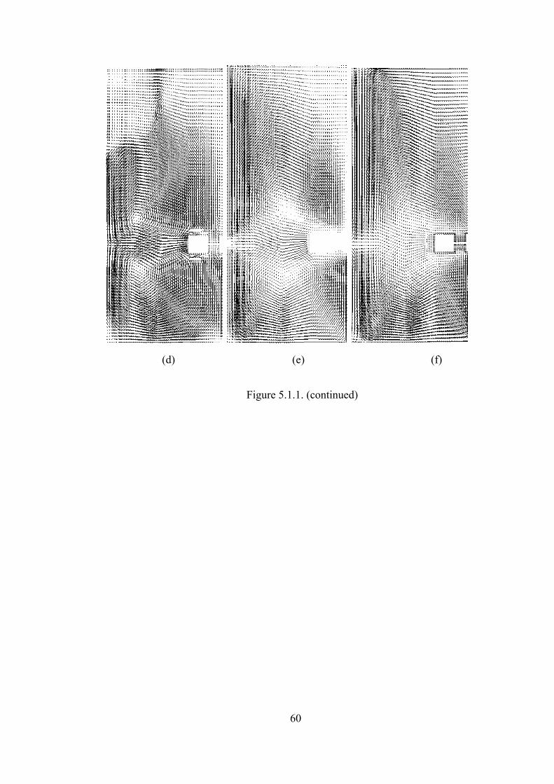
(d) (e) (f)
Figure 5.1.1. (continued)
60

61
5.1.1 Flow pattern in the radial direction
Radial, axial and tangential velocities are also investigated quantitatively at
Reynolds numbers. In addition, values of effective turbulent intensity like turbulent
kinetic energy and turbulent dissipation rate are calculated at Reynold number 10000
and plotted with respect to the radial and axial positions.
The radial velocities are calculated along the impeller blade height in axial
direction at different radial positions, which are normalized by the impeller radius
(R) as shown in Figure 5.1.1.1. Figure 5.1.1.2 depicts the radial velocities at different
Reynolds numbers. In this figure horizontal axis denotes radial velocity component
which is normalized by the impeller tip speed (πNDi), vertical axis, on the other
hand, represents axial position, which is normalized with the impeller blade height
(b) (see Figure 5.1.1.2).
Generally, the center-line radial velocity decreases with increasing radial
distance from impeller which is in agreement with the experimental results from
literature (Wu and Patterson, 1988; Dyster et al., 1993). At high Reynolds numbers
(760-104), on the other hand, center-line radial velocity does not decrease
continuously along radial distance. Instead at r/R=1.32 (8mm away from impeller
blade tip) it makes a local maxima. This effect is a result of the small size of eddies
which are generated by the interaction between the impeller and baffle and they
contain significant portion of the total kinetic energy. Moreover, the differences
between location of the radial and tangential velocity components can be used to
estimate the average eddy size roughly in this region. When the radial velocity is
measured at r/R=2, the effect of eddies disappears and as expected radial velocity
decreases. This trend goes on until Re<300 which correspond to the transition region.
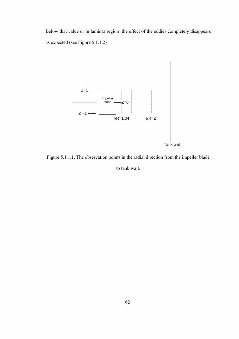
Below that value or in laminar region the effect of the eddies completely disappears
as expected (see Figure 5.1.1.2)
Z=1
Z=-1
Z=0 Impeller
blade
r/R=1.04 r/R=2
Tank wall
Figure 5.1.1.1. The observation points in the radial direction from the impeller blade
to tank wall.
62

Re=10000
-1.5
-1
-0.5
0
0.5
1
1.5
0 0.2 0.4 0.6 0.8
Uθ/Utip
2zb
r/R=1.04
r/R=1.08
r/R=1.16
r/R=1.32
r/R=2
(a)
Re=2069
-1.5
-1
-0.5
0
0.5
1
1.5
0 0.2 0.4 0.6 0.8
Ur/Utip
2zb
r/R=1.04
r/R=1.08
r/R=1.16
r/R=1.32
Figure 5.1.1.2. Axial distribution of the radial velocity profiles at various normalized radial positions at different Reynolds numbers: (a) Re=10000,
(b) Re=2069, (c) Re=760, (d) Re=100, (e) Re=20
(b)
63

Re:760
-1,5
-1
-0,5
0
0,5
1
1,5
-0,2 0 0,2 0,4 0,6 0,8 1 1,2 1,4
Ur/Utip
2zb
r/R=1,04
r/R=1,08
r/R=1,16
r/R=1,32
r/R=2
(c)
Re:100
-1.5
-1
-0.5
0
0.5
1
1.5
0 0.2 0.4 0.6 0.8 1Ur/Utip
2zb
r/R=1.04
r/R=1.08
r/R=1.16
r/R=1.32
r/R=2
(d)
Figure 5.1.1.2. (continued)
64

Re:20
-1.5
-1
-0.5
0
0.5
1
1.5
0 0.2 0.4 0.6 0.8
Ur/Utip
2z b
r/R=1.04
r/R=1.08
r/R=1.16
r/R=1.32
Figure 5.1.1.2. (continued)
(e)
5.1.2. Tangential flow pattern
Tangential velocities at different Reynolds numbers and at various radial
positions are presented in Figure 5.1.2.1. Their magnitudes are higher compared to
the radial components. Also, they are almost symmetrical with respect to the impeller
axis and to the plane of impeller rotation. Tangential velocity components increase
near the impeller but away from the impeller decrease because of the baffles and the
vortices, which are more pronounced as Re increases. Near the baffle region
tangential velocities diminish for all Reynolds number as expected.
In the range where Reynolds number is larger than 100, maximum tangential
velocity appears at the radial distance r/R=1.16 while maximum radial velocity
appears at r/R=1.04. This may be due to vortex formation which changes the velocity
65

66
direction and as a result of this radial velocity is relatively small in the radial distance
of r/R=1.16 where tangential velocity is maximum.
Table 5.1.2.1 shows the maximum value of predicted tangential velocities and
corresponding maximum radial velocities at different Reynolds number. In this table
(Re=2069) tangential velocity can exceed the tip speed due to acceleration of the
fluid over the blades (Stoots and Richard, 1995). The prediction of the maximum
tangential velocity accurately is crucial. Under prediction of the tangential velocity
leads to subsequent under prediction of the radial velocity. The prediction both
maximum tangential and radial velocities agree well with those reported in the
literature (Ranade, 1997).
Table 5.1.2.1. Predicted maximum tangential and radial velocities
Re=10000 Re=2069 Re=760 Re=100 Re=20
Uθ 0.842Utip 1.032Utip 0.760Utip 0.526Utip 0.220Utip
Ur 0.600Utip 0.870Utip 0.622Utip 0.481Utip 0.580Utip

Re=10000
-1.5
-1
-0.5
0
0.5
1
1.5
0 0.2 0.4 0.6 0.8
Uθ/Utip
2zb
r/R=1.04
r/R=1.08
r/R=1.16
r/R=1.32
r/R=2
(a)
Re=2069
-1.5
-1
-0.5
0
0.5
1
1.5
0 0.2 0.4 0.6 0.8
Ur/Utip
2zb
r/R=1.04
r/R=1.08
r/R=1.16
r/R=1.32
(b)
67
Figure 5.1.2.1. Axial distribution of the tangential velocity profiles at various normalized radial positions and various Reynolds numbers: (a) Re=10000, (b)
Re=2069, (c) Re=760, (d) Re=100, (e) Re=20

Re=760
-1,5
-1
-0,5
0
0,5
1
1,5
0 0,2 0,4 0,6 0,8 1
Uθ/Utip
2zb r/R=1,04
r/R=1,08
r/R=1,16
r/R=1,32
r/R=2
(c)
Re=100
-1,5
-1
-0,5
0
0,5
1
1,5
0 0,1 0,2 0,3 0,4 0,5 0,6
Uθ/Utip
2zb r/R=1,04
r/R=1,08
r/R=1,16
r/R=1,32
r/R=2
(d)
Figure 5.1.2.1. (continued)
68

Re=20
-1,5
-1
-0,5
0
0,5
1
1,5
0,05 0,1 0,15 0,2 0,25
Uθ/Utip
2zb r/R=1,04
r/R=1,08
r/R=1,16
r/R=1,32
(e)
Figure 5.1.2.1. (continued)
5.1.3. Axial flow pattern
Axial velocities at different Reynolds numbers and at various radial positions
are demonstrated in Figure 5.1.3.1. Axial velocities are much smaller than the other
components through the impeller stream. In the range of Re>100 axial velocities
fluctuate between negative and positive direction and this trend disappear at radial
distance r/R=2. That is far away from the impeller they almost vanish. This may be
the place where the impeller stream is about to split in to two streams, one flowing
upward, the other flowing downward in to the bulk of the tank (see Figure 5.1.1).As
shown in Figure 5.1.3.1-d-e at laminar region axial velocity components even near
the impeller disappear. At this region radial and tangential velocity components are
dominant.
69

Re=10000
-1.5
-1
-0.5
0
0.5
1
1.5
-0.2 -0.1 0 0.1 0.2
Uz/Utip
2zb
r/R=1.04
r/R=1.08
r/R=1.16
r/R=1.32
r/R=2
(a)
Re=2069
-1.5
-1
-0.5
0
0.5
1
1.5
-0.3 -0.2 -0.1 0 0.1 0.2 0.3
Uz/Utip
2zb
r/R=1.04
r/R=1.08
r/R=1.16
r/R=1.32
(b)
Figure 5.1.3.1. Axial distribution of the axial velocity profiles as a fuction of normalized radial positions at different Reynolds numbers: (a)Re=10000,
(b) Re=2069, (c) Re=760, (d) Re=100, (e) Re=20
70
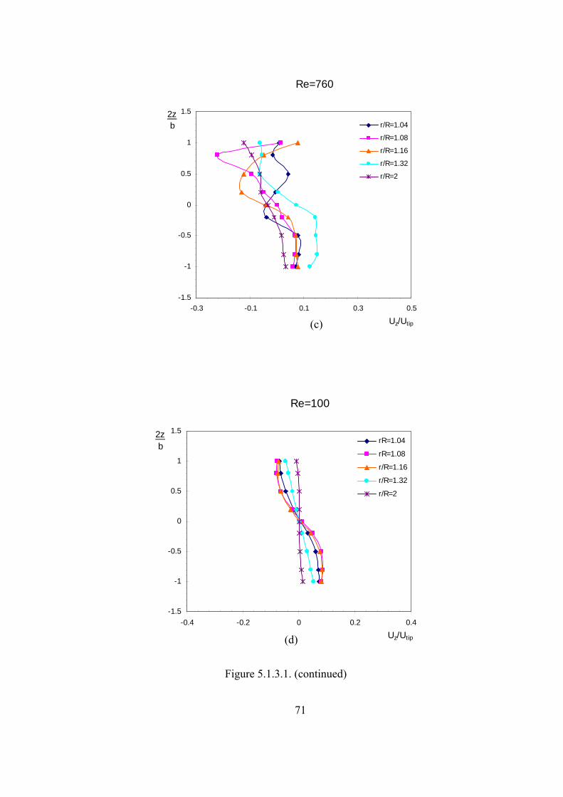
Re=760
-1.5
-1
-0.5
0
0.5
1
1.5
-0.3 -0.1 0.1 0.3 0.5
Uz/Utip
2zb r/R=1.04
r/R=1.08
r/R=1.16
r/R=1.32
r/R=2
(c)
Re=100
-1.5
-1
-0.5
0
0.5
1
1.5
-0.4 -0.2 0 0.2 0.4
Uz/Utip
2zb
rR=1.04
rR=1.08
r/R=1.16
r/R=1.32
r/R=2
(d)
Figure 5.1.3.1. (continued)
71
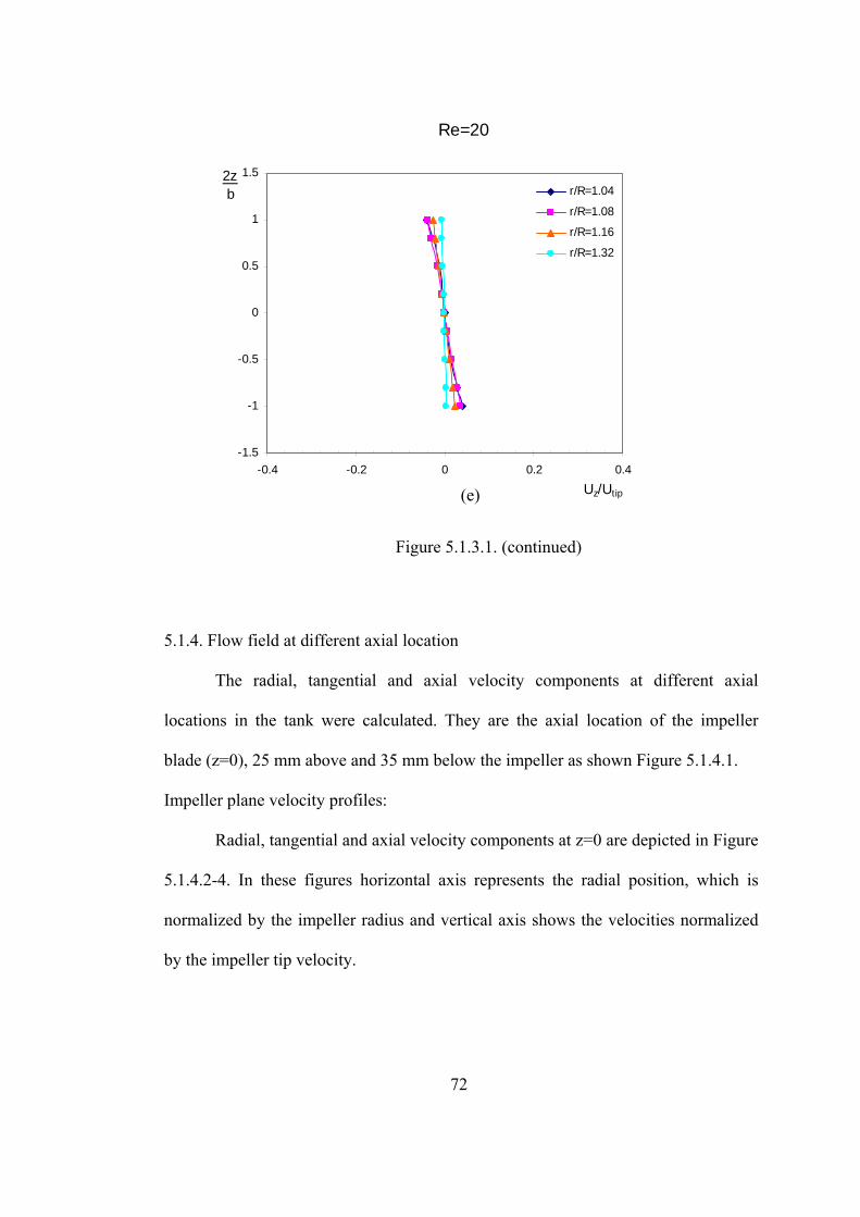
Re=20
-1.5
-1
-0.5
0
0.5
1
1.5
-0.4 -0.2 0 0.2 0.4
Uz/Utip
2zb r/R=1.04
r/R=1.08
r/R=1.16
r/R=1.32
(e)
Figure 5.1.3.1. (continued)
5.1.4. Flow field at different axial location The radial, tangential and axial velocity components at different axial
locations in the tank were calculated. They are the axial location of the impeller
blade (z=0), 25 mm above and 35 mm below the impeller as shown Figure 5.1.4.1.
Impeller plane velocity profiles:
Radial, tangential and axial velocity components at z=0 are depicted in Figure
5.1.4.2-4. In these figures horizontal axis represents the radial position, which is
normalized by the impeller radius and vertical axis shows the velocities normalized
by the impeller tip velocity.
72
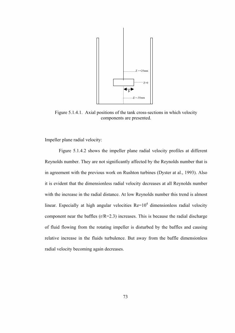
Z=0
R
Z =+25mm
Z =-35mm
Figure 5.1.4.1. Axial positions of the tank cross-sections in which velocity components are presented.
Impeller plane radial velocity:
Figure 5.1.4.2 shows the impeller plane radial velocity profiles at different
Reynolds number. They are not significantly affected by the Reynolds number that is
in agreement with the previous work on Rushton turbines (Dyster at al., 1993). Also
it is evident that the dimensionless radial velocity decreases at all Reynolds number
with the increase in the radial distance. At low Reynolds number this trend is almost
linear. Especially at high angular velocities Re=104 dimensionless radial velocity
component near the baffles (r/R=2.3) increases. This is because the radial discharge
of fluid flowing from the rotating impeller is disturbed by the baffles and causing
relative increase in the fluids turbulence. But away from the baffle dimensionless
radial velocity becoming again decreases.
73
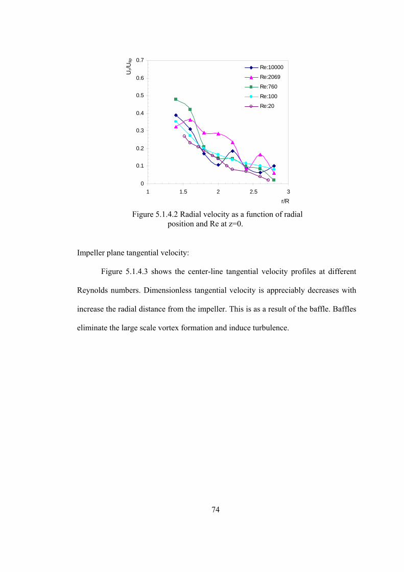
0
0.1
0.2
0.3
0.4
0.5
0.6
0.7
1 1.5 2 2.5 3
r/R
Ur/U
tip
Re:10000
Re:2069
Re:760
Re:100
Re:20
Figure 5.1.4.2 Radial velocity as a function of radial position and Re at z=0.
Impeller plane tangential velocity:
Figure 5.1.4.3 shows the center-line tangential velocity profiles at different
Reynolds numbers. Dimensionless tangential velocity is appreciably decreases with
increase the radial distance from the impeller. This is as a result of the baffle. Baffles
eliminate the large scale vortex formation and induce turbulence.
74
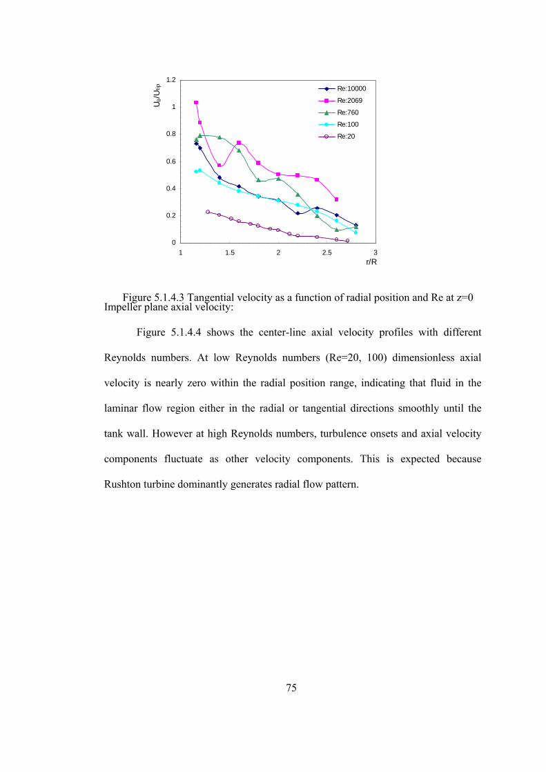
0
0.2
0.4
0.6
0.8
1
1.2
1 1.5 2 2.5 3r/R
Uθ/
Utip Re:10000
Re:2069
Re:760
Re:100
Re:20
Impeller plane axial velocity: Figure 5.1.4.3 Tangential velocity as a function of radial position and Re at z=0
Figure 5.1.4.4 shows the center-line axial velocity profiles with different
Reynolds numbers. At low Reynolds numbers (Re=20, 100) dimensionless axial
velocity is nearly zero within the radial position range, indicating that fluid in the
laminar flow region either in the radial or tangential directions smoothly until the
tank wall. However at high Reynolds numbers, turbulence onsets and axial velocity
components fluctuate as other velocity components. This is expected because
Rushton turbine dominantly generates radial flow pattern.
75
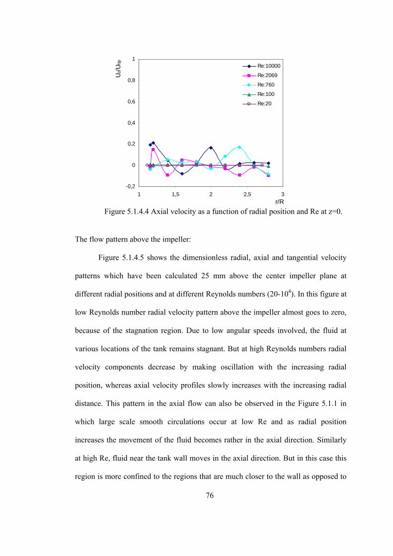
-0,2
0
0,2
0,4
0,6
0,8
1
1 1,5 2 2,5 3r/R
Uz/U
tip Re:10000
Re:2069
Re:760
Re:100
Re:20
The flow pattern above the impeller:
Figure 5.1.4.4 Axial velocity as a function of radial position and Re at z=0.
Figure 5.1.4.5 shows the dimensionless radial, axial and tangential velocity
patterns which have been calculated 25 mm above the center impeller plane at
different radial positions and at different Reynolds numbers (20-104). In this figure at
low Reynolds number radial velocity pattern above the impeller almost goes to zero,
because of the stagnation region. Due to low angular speeds involved, the fluid at
various locations of the tank remains stagnant. But at high Reynolds numbers radial
velocity components decrease by making oscillation with the increasing radial
position, whereas axial velocity profiles slowly increases with the increasing radial
distance. This pattern in the axial flow can also be observed in the Figure 5.1.1 in
which large scale smooth circulations occur at low Re and as radial position
increases the movement of the fluid becomes rather in the axial direction. Similarly
at high Re, fluid near the tank wall moves in the axial direction. But in this case this
region is more confined to the regions that are much closer to the wall as opposed to
76

the low Re cases. Tangential velocities at high Reynolds number increases until a
certain radial position (r/R=1.4) and then start to decrease towards zero. At low
Reynolds numbers, along the radial distance there is not any variation of tangential
velocity components.
-0,3
-0,1
0,1
0,3
0,5
0,7
0,9
0 0,5 1 1,5 2 2,5 3r/R
Ur/U
tip Re:10000
Re:2069
Re:760
Re:100
Re:20
(a)
-0,5
-0,3
-0,1
0,1
0,3
0,5
0,7
0,9
0 0,5 1 1,5 2 2,5 3r/R
Uz/
Utip Re:10000
Re:2069
Re:760
Re:100
Re:20
(b)
Figure 5.1.4.5. Velocity components as a function of radial position and Re above the impeller (z=+25 mm) (a) radial velocity, (b) axial velocity, (c) tangential velocity.
77
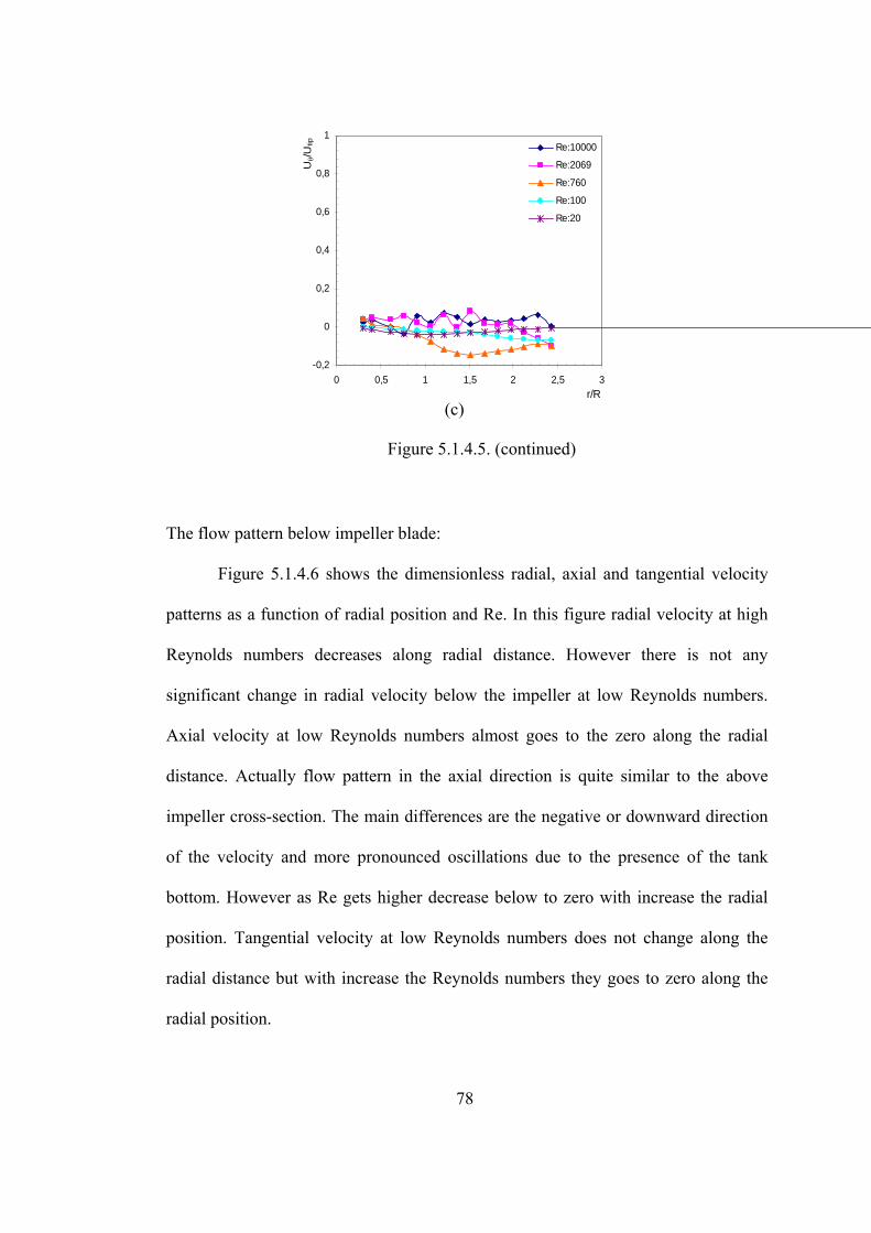
-0,2
0
0,2
0,4
0,6
0,8
1
0 0,5 1 1,5 2 2,5 3r/R
Uθ/U
tip Re:10000
Re:2069
Re:760
Re:100
Re:20
Figure 5.1.4.5. (continued)
(c)
The flow pattern below impeller blade:
Figure 5.1.4.6 shows the dimensionless radial, axial and tangential velocity
patterns as a function of radial position and Re. In this figure radial velocity at high
Reynolds numbers decreases along radial distance. However there is not any
significant change in radial velocity below the impeller at low Reynolds numbers.
Axial velocity at low Reynolds numbers almost goes to the zero along the radial
distance. Actually flow pattern in the axial direction is quite similar to the above
impeller cross-section. The main differences are the negative or downward direction
of the velocity and more pronounced oscillations due to the presence of the tank
bottom. However as Re gets higher decrease below to zero with increase the radial
position. Tangential velocity at low Reynolds numbers does not change along the
radial distance but with increase the Reynolds numbers they goes to zero along the
radial position.
78
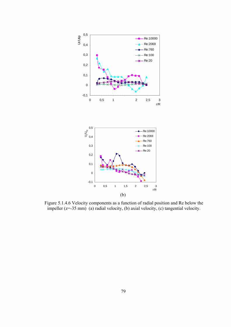
-0,1
0
0,1
0,2
0,3
0,4
0,5
0 0,5 1
1(a) ,5 2 2,5 3r/R
Ur/U
tip Re:10000
Re:2069
Re:760
Re:100
Re:20
-0,1
0
0,1
0,2
0,3
0,4
0,5
0 0,5 1 1,5 2 2,5 3r/R
U z/Utip Re:10000
Re:2069
Re:760
Re:100
Re:20
Figure 5.1.4.6 Velocity components as a function of radial position and Re below the impeller (z=-35 mm) (a) radial velocity, (b) axial velocity, (c) tangential velocity.
(b)
79
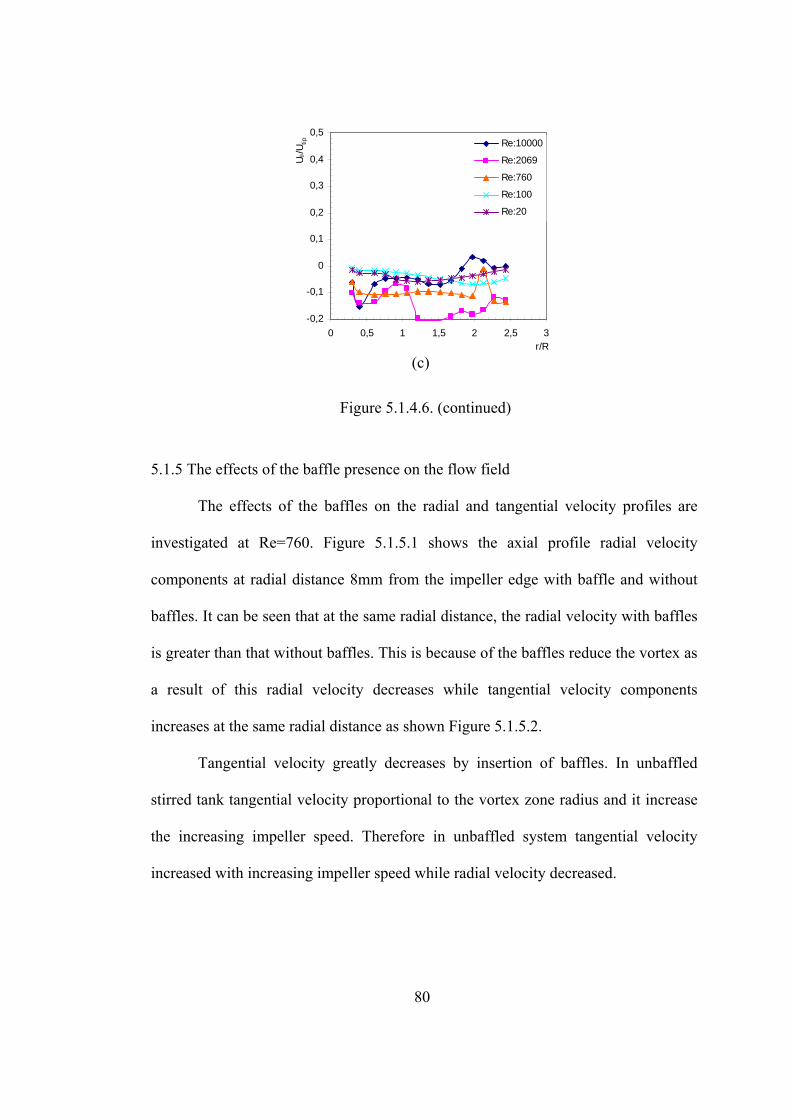
-0,2
-0,1
0
0,1
0,2
0,3
0,4
0,5
0 0,5 1 1,5 2 2,5 3r/R
U θ/U
tip Re:10000
Re:2069
Re:760
Re:100
Re:20
(c)
Figure 5.1.4.6. (continued)
5.1.5 The effects of the baffle presence on the flow field
The effects of the baffles on the radial and tangential velocity profiles are
investigated at Re=760. Figure 5.1.5.1 shows the axial profile radial velocity
components at radial distance 8mm from the impeller edge with baffle and without
baffles. It can be seen that at the same radial distance, the radial velocity with baffles
is greater than that without baffles. This is because of the baffles reduce the vortex as
a result of this radial velocity decreases while tangential velocity components
increases at the same radial distance as shown Figure 5.1.5.2.
Tangential velocity greatly decreases by insertion of baffles. In unbaffled
stirred tank tangential velocity proportional to the vortex zone radius and it increase
the increasing impeller speed. Therefore in unbaffled system tangential velocity
increased with increasing impeller speed while radial velocity decreased.
80
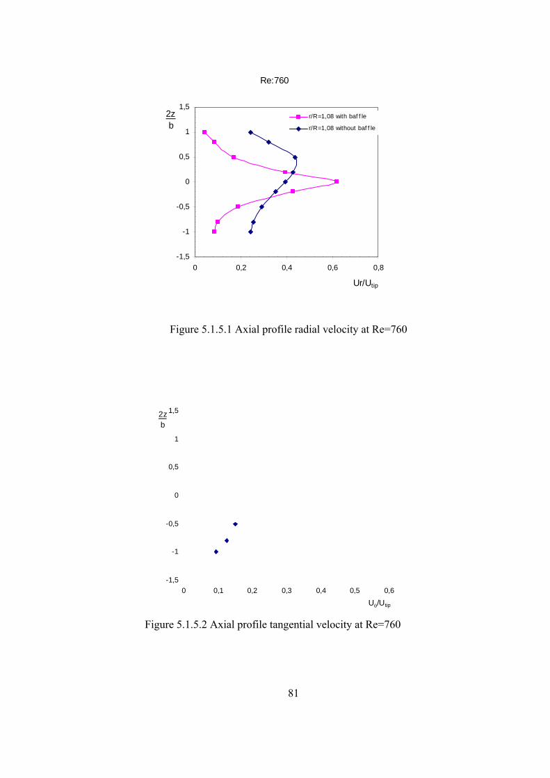
Re:760
-1,5
-1
-0,5
0
0,5
1
1,5
0 0,2 0,4 0,6 0,8
Ur/Utip
2zb
r/R=1,08 with baf f le
r/R=1,08 without baf f le
=760
r/R=1,08 w ith baffle
r/R=1,08 w ithout baffle
Figure 5.1.5.1 Axial profile radial velocity at Re=760
Re
-1,5
-1
-0,5
0
0,5
1
1,5
0 0,1 0,2 0,3 0,4 0,5 0,6
Uθ/Utip
2z
b
81
Figure 5.1.5.2 Axial profile tangential velocity at Re=760
5.1.6 Kinetic energy and kinetic energy dissipation rate
Turbulent kinetic energy and turbulent dissipation rate are evaluated at
Reynold number 104 using k-ε model. The value of k calculated from equation
(5.1.6.1):
)(21 222
zr VVVk ++= θ (5.1.6.1)
where 2rV , 2
θV , 2zV are the fluctuating velocities radial, tangential and axial direction
respectively. Figure 5.1.6.1 depicts the turbulent kinetic energy, which is normalized
by U2tip at the various radial locations from the blade edge. Near the impeller change
in the k values as a function of axial locations occur stronger than those regions of
more distant regions. Higher turbulent kinetic energies in vicinity of the impeller can
be expected. The fluctuations in the k values with respect to axial position indicate
that there are regions where fluid has a higher kinetic energy than others which can
be explained through the turbulent eddies having characteristic length and velocity
scales of the impeller height and velocity, respectively.
82
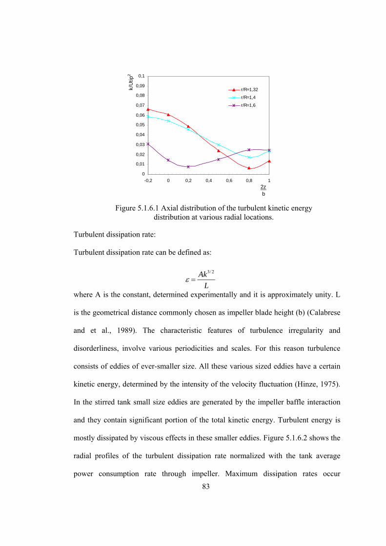
0
0,01
0,02
0,03
0,04
0,05
0,06
0,07
0,08
0,09
0,1
-0,2 0 0,2 0,4 0,6 0,8 12zb
k/U
tip2
r/R=1,32
r/R=1,4
r/R=1,6
Turbulent dissipation rate:
Figure 5.1.6.1 Axial distribution of the turbulent kinetic energy distribution at various radial locations.
Turbulent dissipation rate can be defined as:
where A is the constant, determined experimentally and it is approximately unity. L
is the geometrical distance commonly chosen as impeller blade height (b) (Calabrese
and et al., 1989). The characteristic features of turbulence irregularity and
disorderliness, involve various periodicities and scales. For this reason turbulence
consists of eddies of ever-smaller size. All these various sized eddies have a certain
kinetic energy, determined by the intensity of the velocity fluctuation (Hinze, 1975).
In the stirred tank small size eddies are generated by the impeller baffle interaction
and they contain significant portion of the total kinetic energy. Turbulent energy is
mostly dissipated by viscous effects in these smaller eddies. Figure 5.1.6.2 shows the
radial profiles of the turbulent dissipation rate normalized with the tank average
power consumption rate through impeller. Maximum dissipation rates occur
LAk 2/3
=ε
83

approximately at the mid point of the impeller stream where fraction of the small size
eddies is high.
5
7
9
11
13
15
17
19
21
23
1 1,2 1,4 1,6 1,8 2 2,2
ε/ε'
r/R
Figure 5.1.6.2 Radial distribution of the turbulent kinetic energy dissipation rate.
5.2 Power Number
Second part of our study is on the determination of the power consumption
and the effects of the baffle length on the power number at different Reynolds
numbers. Several shape factors have strong effect on the power number which are
given in Chapter 2. In this section only one of those parameters, baffle length, is
considered since it has been reported as the most effective parameter on the power
consumption among the shape factors in the literature (Holland and Chapman, 1996).
Figure 5.2.1 shows the experimentally obtained power number versus Re,
which is plotted in log-log scale for a standard tank configuration. Figure 5.2.1
shows that at low Reynolds numbers the plot is linear. In this range the viscous
forces dominate the system. As the Reynolds number increases the flow changes
from laminar to turbulent, the power curve becomes horizontal. For lower impeller
84
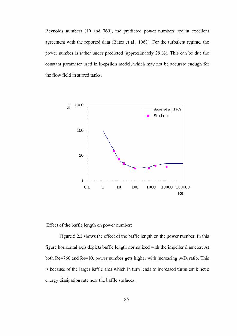
Reynolds numbers (10 and 760), the predicted power numbers are in excellent
agreement with the reported data (Bates et al., 1963). For the turbulent regime, the
power number is rather under predicted (approximately 28 %). This can be due the
constant parameter used in k-epsilon model, which may not be accurate enough for
the flow field in stirred tanks.
1
10
100
1000
0,1 1 10 100 1000 10000 100000Re
Np
Bates et al., 1963
Simulation
Figure 5.2.1 Power number as a function of Re for standart tank configuration
Effect of the baffle length on power number:
Figure 5.2.2 shows the effect of the baffle length on the power number. In this
figure horizontal axis depicts baffle length normalized with the impeller diameter. At
both Re=760 and Re=10, power number gets higher with increasing w/Di ratio. This
is because of the larger baffle area which in turn leads to increased turbulent kinetic
energy dissipation rate near the baffle surfaces.
85

2
3
4
5
6
7
8
0 0,2 0,4 0,6w/Di
Np
Re=10
Re=760
86
Figure 5.2.2. Effect of the baffle length on the power number
87
CHAPTER 6
CONCLUSIONS
The flow field and power consumption generated by Ruhton turbine impeller have
been calculated using computational fluid dynamics techniques in conjuction with a
multiple frame of reference method for various Reynolds numbers in both laminar
and turbulent regime. The results obtained in this study allow one to draw the
following conclusions:
1. Multiple frame of reference method has demonstrated that it is able to
simulate the flow in stirred tanks and to produce realistic predictions.
2. In the r-z plane a strong radially oriented flow is observed to emerge from the
impeller, producing two main recirculation flows, one above and the other
below the impeller plane. Location of the circulation loops’ centers change
with increasing Reynolds numbers and move closer to the impeller plane.
3. Axial distribution of the center-line radial velocity components decrease with
increasing radial distance from the impeller. But tangential velocity remain
higher than the radial velocity and increase until radial distance r/R=1.16.
After this location decreases with increasing radial distance. The axial
velocity component is much smaller than the other components through the
impeller stream and far away from the impeller it almost vanishes.

88
4. Impeller plane radial velocity is not significantly affected by the Reynolds
numbers. Tangential velocity appreciable decrease at higher radial positions
or away from the impeller region for all Re numbers. Axial velocity is found
nearly zero especially in the laminar region.
5. At low Re numbers, radial velocity above the impeller becomes almost zero
because of the stagnation region. However Tangential velocity is found to
increase until a certain radial position (r/R=1.4) and then starts to decrease
towards zero. Axial velocity diminishes along the radial position.
6. Radial velocity decreases below the impeller along the radial distance but
tangential velocity does not change. Axial velocity exhibits similar
characteristics to the axial velocity above the impeller.
7. Radial velocity component in an unbaffled vessel significantly decreases
while tangential velocity gets higher at the same radial position.
8. Turbulent kinetic energy decreases as a function of radial position at
Re=10000. In addition, maximum turbulent kinetic energy dissipation rate is
found approximately at the mid point of the impeller stream where fraction of
the small sized eddies is higher compared to the other tank locations.
9. Power curve is found in excellent agreement with the experimental data.
Using larger baffle lengths lead to higher power consumption or power
number.

89
REFERENCES
Abbott, Michael B., 1989, “Computational fluid dynamics: an introduction for
engineers”, Longman Scientific & Technical New York.
Bakker A., K. J. Mysers, R.W. Ward and C.K. Lee, 1996, “The Laminar and
Turbulence Flow Pattern of Pitched Blade Turbine”, Trans. I. Chem. E. 74, pp. 485-
491.
Bakker, A. and Van den Akker, H. E. A., 1992, “A computational study on
dispersing gas in stirred reactor, in Fluid Mechanics of Mixing”, Kluwer Academic
Publishers.
Bakker, A., R.D. Laroche, M.H. Wang and R.V. Calabrese, 1997, “Sliding Mesh
Simulation of Laminar Flow in Stirred Reactors”, Trans. Inst. Chem. Eng. 75, pp. 42-
44.
Bates, R.L., Fondy, P.L., and Corpstein, R.R., 1963, “An examination of some
geometrical parameters of impeller power”, Ind. Eng. Chem. Proc. Des. Dev., 2: 310.
C. Hirsch, 1997, “Numerical Computation of Internal and External Flows”, John
Wiley & Sons.
Brucato, A., Ciofalo, M., Grisafi, F. and Micale, G., 1998, “Numerical prediction of
flow fields in baffled stirred vessels: A comparison of alternative modeling
approaches”, Chem.Engng Sci., 53, pp. 3653-3684.
90
Calabrese, R. and Stoots, C. M., 1989, “Flow in the impeller region of a stirred tank”,
Chem. Eng. Prog., pp.43-50.
D.H. Norrie and G. de Vries, 1978, “An Introduction to Finite Element Analysis”,
Academic press New York.
DeSouza, A. ande Brezina, V., 1972, “Fluid Dynamics and Flow Patterns in Stirred
Tanks with a Turbine Impeller”, Can.J. Chem. Engng., 50, pp. 15-23.
Dyster, K. N., Koutsakos, E., Jaworski, Z. and Nienow, A.E., 1993, “An LDA study
of the radial discharge velocities generated by a Rushton turbine”, Chem. Engng Res.
Des., 71, 11.
Fluent, 2000, “Journal articles by Fluent software users”, Fluent.
Harvey, P.S. and Greaves, M., 1982, “Turbulent flow in agitated vessel”, Trans.
IChemE., 60, pp. 195-210.
Holland, F. A., Chapman, F.S., 1966, “Liquid Mixing and Processing in Stirred
Tanks”, Lever Brothers Company, New York.
J. N. Reddy, 1993, “An Introduction to the Finite element Method”, McGraw-Hill.
J. O. Hinze, 1975, “Turbulence”, McGraw-Hill.
Jaworski, Z., Nienow, A.W., Koutsakos, E., Dyster, K., 1996, “An LDA Study of
Turbulent Flow in a Baffled Vessel Agitated by an Axial, Down-pumping Hydrofil
Impeller”, Can. J. Chem. Eng., 74, pp. 3-15.
Joel H. Ferziger and M. Peric, 1996, “Computational Methods for Fluid Dynamics”,
Springer-Verlag.

91
Kresta, S.M. and P.E. Wood, 1991, “Prediction of Three Dimensional Turbulence
Flow in Stirred Tanks”, AIChE., 37, pp. 448-460.
Kresta, S.M. and P.E. Wood, 1993,”The Flow Field Produced by a Pitched Blade
Turbine: Characterization of the Turbulence and Estimation of Dissipation Rate”,
Chem. Eng. Sci., 48, pp. 1761-1773.
Lee, K. C., Ng, K. and Yanneskis, M., 1996, “Sliding mesh predictions of turbulent
flow around Rushton impellers”, IChemE Symp. Ser. 140, 47-58.
M. Griebel, T. Dornseifer and T. Neunhoeffer, 1998, “Numerical Simulation in Fluid
Dynamics”, SIAM.
Nagata, S., 1975, “Mixing Principle and Applications”, Wiley New York.
Naude, I., Xuereb, C. and Bertrand, J., 1998, “Direct Prediction of the Flows Induced
by Propeller in an Agitated Vessel Using an Unstructured Mesh”, Can. J. Chem.
Eng., 76, pp. 631-640.
Periclous, K.A. and Patel, M. K., 1987, “The modeling of tangential and axial
agitators in chemical reactors”, PhysicoChem. Hydrodyn., 8, pp. 105-123.
Placek, J., Tavlarides, L. L., Smith, G. W. and Fort, I., 1986, “Turbulent flow in
stirred tanks”, AIChE, 32, 1771.
Ranade, V.V. and Dommeti, S.M.S., 1996, “Computational Snapshot of flow
Generated by Axial Impellers in Baffled Stirred Vessel”, Trans. IChemE., 74, A, pp.
476-484.
Ranade, V.V. and Joshi, J.B., 1990b, “Flow generated by a Disc Turbine: Part II
Mathematical Modeling and Comparison with Experimental Data”, Trans.IhemE.,
68, A, pp. 34-50.
92
Ranade, V.V. Joshi, J.B. and Marathe, A.G., 1989, “Flow generated by pitched blade
turbines II: simulation using k-epsilon model”, Chem. Engng. Comm., 81, pp. 225-
248.
Ranade, V.V., 1997, “An efficient computational model for simulating flow in stirred
vessels: a case of Rushton turbine”, Chem.Engng Sci., 52, pp. 4473-4484.
Ranade, V.V.and Joshi, J.B., 1990a, “Flow generated by a Disc Turbine: Part I
Experimental”, Trans.IchemE., 68, A, pp. 19-33.
Roache, Patrick J., 1976, “Computational Fluid Dynamics”, Hermose.
Sahu, A.K., Kumar, P., Patwardhan, A.W., Joshi, J.B., 1999, “CFD modeling and
mixing in stirred tanks”, Chem.Engng Sci., 54, pp. 2285-2293.
Stoots, C. M. and Calabrese, R.V., 1995, “Mean velocity field relative to a Rushton
turbine blade”, A.I.Ch.E. J., 41, 1.
Tatterson, G.B., 1994, “Scaleup and Design of Industrial Mixing Process”, McGraw-
Hill, New York.
Versteeg, H. K. and Malalaseke, W., 1995, “An introduction to computational Fluid
Dynamics: The finite volume method”, Addison-Wesley.
Wu, H., G.K. Patterson and M. Van Doorn, 1989, “Distribution of Turbulent Flow
Parameters in a Stirred Mixer”, Chem. Eng. Sci., 44, pp. 2207-2221.
Xu, Y. and McGrath, G., 1986, “Computational Fluid Dynamics Predictions of
Stirred Tank Flows”, Trans. IChemE., 74, pp.471-475.
Related Documents


