Numerical investigation of bubbles in channel flow Implementation and analysis of the influence of bubbles injection on the drag of a ship Master’s thesis in Nordic Master in Maritime Engineering RÉMY LE GUEN Department of Shipping and Marine Technology CHALMERS UNIVERSITY OF TECHNOLOGY Gothenburg, Sweden 2016

Welcome message from author
This document is posted to help you gain knowledge. Please leave a comment to let me know what you think about it! Share it to your friends and learn new things together.
Transcript

Numerical investigation of bubbles inchannel flowImplementation and analysis of the influence of bubblesinjection on the drag of a ship
Master’s thesis in Nordic Master in Maritime Engineering
RÉMY LE GUEN
Department of Shipping and Marine TechnologyCHALMERS UNIVERSITY OF TECHNOLOGYGothenburg, Sweden 2016


Master’s thesis X-16/353
Numerical investigation of bubbles in channel flow
Implementation and analysis of the influence of bubbles injection onthe drag of a ship
RÉMY LE GUEN
Department of Shipping and Marine TechnologyChalmers University of Technology
Gothenburg, Sweden 2016

Numerical investigation of bubbles in channel flowImplementation and analysis of the influence of bubbles injection on the drag of ashipRÉMY LE GUEN
© RÉMY LE GUEN, 2016.
Supervisor:RICKARD BENSOW, Department of Shipping and Marine TechnologySVERRE STEEN, Institutt for marin teknikk, NTNU
Master’s Thesis 2016:X-16/353Department of Shipping and Marine TechnologyChalmers University of TechnologySE-412 96 GothenburgTelephone +46 31 772 1000
Cover: Result of a 3D-simulation performed in a Lagrangian framework for bubblesof 1mm diameters.
Typeset in LATEXPrinted by ReproserviceGothenburg, Sweden 2016
iv

Numerical investigation of bubbles in channel flowImplementation and analysis of the influence of bubbles injection on the drag of ashipRÉMY LE GUENDepartment of Shipping and Marine TechnologyChalmers University of Technology
AbstractThis master’s thesis aims to study the numerical methods that can simulate theinfluence of injection of air bubbles under a ship’s hull. The geometry of the hullis simplified to a flat plate and the analysis is only done in two dimensions. Anemphasis is given into the prediction of the reduction of the viscous resistance thatis observed in experiments. This study is carried out using CFD analysis with thesoftware OpenFOAM.Two frameworks, Eulerian-Eulerian and Eulerian-Lagrangian, that allows the simu-lation of a multiphase flow are set-up and the assumptions behind all the requiredmodels are explained. The simulations predicts a gain of efficiency between 0% and15% depending on the diameter of the bubbles. Some differences in the results pro-duced by the two different methods are highlighted and guidance is given on whichsolver to use for a given case depending on the diameter and the concentration ofthe bubbles below the plate.
Keywords: multiphase simulation, OpenFOAM, drag reduction, Lagrangian ParticleTracking.
v


AcknowledgementsFirst I would like to thanks my supervisor Prof. Rickard Bensow to have helpedme setting-up the subject of the thesis and guiding me through the process. I wantalso to thank PhD student Sankar Menon Cherubala Pathayapura to have helpedme for the practical matters all along the work.
To Prof. Sverre Steen for having been my NTNU supervisor and for having givenme the interest in naval hydrodynamics during my first year of master.
I would also like to thank the staff of the "École Centrale de Lyon" (and especiallythe international office staff) who gave me the opportunity to realize this doubledegree.
To Prof. Poul Andersen for coordinating this amazing programme that is the NordicMaster in Maritime Engineering and for helping during the problem encountered.
Enfin, j’aimerais remercier mes amis et ma famille pour m’avoir supporté dans cetteaventure.
Le Guen Rémy, Gothenburg, June 2016
vii


Contents
List of Figures xi
List of Tables xiii
Nomenclature xv
1 Introduction 1
2 Mathematical formulation 32.1 Shape of the bubble . . . . . . . . . . . . . . . . . . . . . . . . . . . . 3
2.1.1 The bubble’s regimes . . . . . . . . . . . . . . . . . . . . . . . 32.1.2 Characterization of the regimes . . . . . . . . . . . . . . . . . 4
2.2 Dispersed multiphase flow model . . . . . . . . . . . . . . . . . . . . 62.2.1 Eulerian-Eulerian framework . . . . . . . . . . . . . . . . . . . 62.2.2 Eulerian-Lagrangian framework . . . . . . . . . . . . . . . . . 72.2.3 Comparison between the two formulations . . . . . . . . . . . 8
2.3 The closure term . . . . . . . . . . . . . . . . . . . . . . . . . . . . . 82.3.1 Drag force . . . . . . . . . . . . . . . . . . . . . . . . . . . . . 92.3.2 Virtual mass force . . . . . . . . . . . . . . . . . . . . . . . . 102.3.3 Lift Force . . . . . . . . . . . . . . . . . . . . . . . . . . . . . 102.3.4 Wall lubrication force . . . . . . . . . . . . . . . . . . . . . . . 112.3.5 Turbulent dispersion force . . . . . . . . . . . . . . . . . . . . 112.3.6 Collision force . . . . . . . . . . . . . . . . . . . . . . . . . . . 12
2.4 Turbulence . . . . . . . . . . . . . . . . . . . . . . . . . . . . . . . . . 122.4.1 The fluid phase turbulence (k − ε model) . . . . . . . . . . . . 122.4.2 Influence of the bubbles on the turbulence (Lahey model) . . . 132.4.3 The turbulent fluctuation velocity . . . . . . . . . . . . . . . . 14
2.5 Coalescence and breakage processes . . . . . . . . . . . . . . . . . . . 142.5.1 Coalescence and breakage mechanisms . . . . . . . . . . . . . 152.5.2 Implementation in a multiphase flow formulation . . . . . . . 162.5.3 Models for the formation and loss rate terms . . . . . . . . . . 17
3 Numerical implementation 213.1 Eulerian-Eulerian implementation . . . . . . . . . . . . . . . . . . . . 21
3.1.1 The mass conservation equation . . . . . . . . . . . . . . . . . 213.1.2 The momentum equation . . . . . . . . . . . . . . . . . . . . . 223.1.3 The pressure correction equation . . . . . . . . . . . . . . . . 23
ix

Contents
3.2 Eulerian-Lagrangian implementation . . . . . . . . . . . . . . . . . . 243.2.1 Equations in the Eulerian and Lagrangian frame . . . . . . . . 243.2.2 Implementation of the collision . . . . . . . . . . . . . . . . . 26
3.3 Implementation of the problem . . . . . . . . . . . . . . . . . . . . . 263.3.1 Geometry and physical properties . . . . . . . . . . . . . . . . 273.3.2 Boundary conditions . . . . . . . . . . . . . . . . . . . . . . . 273.3.3 Meshing, discretization scheme and closure models . . . . . . . 293.3.4 Post-processing of the results . . . . . . . . . . . . . . . . . . 30
4 Results and discussions 334.1 General results . . . . . . . . . . . . . . . . . . . . . . . . . . . . . . 33
4.1.1 Behaviour of a bubbly flow . . . . . . . . . . . . . . . . . . . . 334.1.2 Behaviour without injection of bubbles . . . . . . . . . . . . . 354.1.3 Comparison between the solvers . . . . . . . . . . . . . . . . . 37
4.2 Sensitivity of the results regarding the different parameters . . . . . . 394.2.1 Influence of the turbulence model . . . . . . . . . . . . . . . . 394.2.2 Influence of breaking/coalescence process . . . . . . . . . . . . 40
4.3 Influence of the diameter of the bubble on the solution . . . . . . . . 424.3.1 Influence of the diameter in a Lagrangian formulation . . . . . 424.3.2 Comparison with the Eulerian formulation . . . . . . . . . . . 444.3.3 Influence of the rate flow . . . . . . . . . . . . . . . . . . . . . 46
5 Conclusion 49
Bibliography 51
A Definition of the geometry and the boundary conditions I
B twoPhaseEulerFoam configuration files VII
C DPMFoam configuration files XIII
x

List of Figures
1.1 The three major categories for air lubrication . . . . . . . . . . . . . 1
2.1 Sketches of various bubble shapes observed in infinite Newtonian liquids 42.2 Bubble regimes depending on the dimensionless numbers . . . . . . . 52.3 Coalescence of two bubbles . . . . . . . . . . . . . . . . . . . . . . . . 152.4 Major bubble interaction mechanisms in a bubbly flow . . . . . . . . 18
3.1 Pseudo code of the solution procedure of twoPhaseEulerFoam . . . . 223.2 Pseudo code of the solution procedure of DPMFoam and MPPICFoam . . 253.3 2-D geometry of the problem . . . . . . . . . . . . . . . . . . . . . . . 283.4 The mesh used for the study . . . . . . . . . . . . . . . . . . . . . . . 31
4.1 Distribution of the void fraction over the domain . . . . . . . . . . . 344.2 Distribution of the quantities wrt. the distance to the wall . . . . . . 344.3 Spatial distribution of the Tadaki number . . . . . . . . . . . . . . . 354.4 Comparison of the quantities with and without bubbles . . . . . . . . 364.5 Typical output of a Lagrangian solver . . . . . . . . . . . . . . . . . . 374.6 Comparison of the quantities between the tree solvers wrt. the dis-
tance to the wall . . . . . . . . . . . . . . . . . . . . . . . . . . . . . 384.7 Comparison of the different quantities between solvers . . . . . . . . . 404.8 Average diameter of the bubble . . . . . . . . . . . . . . . . . . . . . 414.9 Gain of efficiency wrt. diameter with the LPT solver . . . . . . . . . 424.10 Void fraction distribution for different diameters . . . . . . . . . . . . 434.11 Comparison of the quantities wrt. the diametre of the bubbles . . . . 444.12 Comparison of the skin friction computed by the two solvers . . . . . 454.13 Lateral void-fraction for different diameters . . . . . . . . . . . . . . . 464.14 Skin friction coefficient wrt. rate flow for 1mm bubbles . . . . . . . . 464.15 Skin friction coefficient wrt. rate flow for different diameter of bubbles 47
xi

List of Figures
xii

List of Tables
2.1 Default coefficients of the k − ε model . . . . . . . . . . . . . . . . . 13
3.1 Physical properties of the phases . . . . . . . . . . . . . . . . . . . . 273.2 Boundary conditions for the inlets and outlet . . . . . . . . . . . . . . 293.3 Boundary conditions for the wall and stream patches . . . . . . . . . 293.4 Choice of the models for the closure interface . . . . . . . . . . . . . . 303.5 Choice of the discretization schemes . . . . . . . . . . . . . . . . . . . 30
4.1 Properties of the Eulerian-Eulerian simulation . . . . . . . . . . . . . 334.2 Properties of the simulation without injection of bubbles . . . . . . . 354.3 Skin friction coefficient with and without bubbles . . . . . . . . . . . 364.4 Properties of the LPT simulations . . . . . . . . . . . . . . . . . . . . 374.5 Comparison of the friction coefficients . . . . . . . . . . . . . . . . . . 384.6 Properties of the turbulent simulations . . . . . . . . . . . . . . . . . 394.7 Properties of the IAC simulation . . . . . . . . . . . . . . . . . . . . 41
xiii

List of Tables
xiv

Nomenclature
Latin symbols
Symbol Dimension DescriptionCd – Drag coefficientCF – Friction skin coefficientCl – Lift coefficientCtd – Turbulent diffusion coefficientCvm – Virtual mass coefficientCwl – Wall lubrication coefficientD [m] Diameter of the bubbleDs [m] Sauter diameter of the bubble~g [m.s−2] Gravity vectork [m2.s−2] Turbulent kinetic energy~n – Wall normal vectoru [m.s−1] Turbulent fluctuation of the velocity~U [m.s−1] VelocityU [m.s−1] Mean velocity~Ur [m.s−1] Relative velocity ~Ur = ~Ub − ~Ufy [m] Near wall distancey+ – Dimensionless distance from the wall
Greek symbols
Symbol Dimension Descriptionα – Void fractionε [m2.s−3] Turbulent energy dissipationµ [Pa.s] Dynamic viscosityν [m2.s−1] Kinematic viscosityνT [m2.s−1] Turbulent kinematic viscosityρ [kg.m−3] Densityτ [N.m−2] Shear stressσ – surface tensionΦ [m−3] Source/sink in the IAC equationφ – Aspect ratio of a bubble
xv

Nomenclature
Adimensional numbers
Symbol Dimension DescriptionReb – Reynold Bubble numberEo – Eotvos numberWe – Weber numberMo – Morton number
Subscripts
Symbol Descriptionb Bubble phasef Fluid phasew Wall
Acronyms
Acronym DescriptionCFD Computational Fluid DynamicsIAC Interface area concentrationLPT Lagrangian Particle TrackingMPPIC MultiPhase Particle-In-Cell methodMULES Multidimensional Universal Limiter with Explicit SolutionRANS Reynolds-averaged Navier–Stokes equations
xvi

1Introduction
Due to environmental concerns and the rising fuel cost, the shipping industry aimsfor a better fuel efficiency for their vessels. One of the way to achieve this is toreduce the resistance of the ships. The frictional resistance – the dominant resistancecomponent for low-Froude number ships – is difficult to reduce as it strongly dependson the wetted surface of the ship. Thus, the interest in techniques that reduce thefrictional resistance has increased over the last two decades and several researchprojects in the USA, Europe and Asia have investigated the possibility of reducingfrictional drag by using air lubrication. This technique can be divided into threemajor categories (Ceccio and Simo, 2011) as illustrated in figure 1.1: Bubble DragReduction (a); Air Layer Drag Reduction (b) and Partial Cavity Drag Reduction(c). This thesis will only be focused on dispersed bubbles in the flow.
Figure 1.1: The three major categories for air lubrication (extracted from Ceccioand Simo, 2011, fig. 0.1)
In 2011, the Mitsubishi Air Lubrication System (MALS) was the first bubble dragreduction system in the world to be applied to a newly built ship, and is said bythe company to have resulted in a substantial reduction in the ship’s resistance.Likewise, a project about air cavity ships is currently carried out by Chalmers 1
and aims to “study the optimum configuration of a stable air cavity with the leastdrag force and air flow rate through experimental investigation in water tunnel andcomputational fluid dynamics (CFD) technique”.
In figure 1.1.c, the closure of the air cavity involves the creation and the ejectionof air bubbles. In a way, the presence of bubbles can be beneficial and lead to an
1https://www.chalmers.se/en/projects/Pages/Energy-Efficient-Air-Cavity-Ships.aspx
1

1. Introduction
additional reduction of the drag but it can also lead to a loss of efficiency if thebubbles reduce the thrust of the propeller.
There are uncertainties about the typical gain of efficiency expected from the in-jection of bubbles along the hull. If some experiments predict a reduction of 50 %– and sometimes even up to 80 % – in the viscous resistance (Sanders et al., 2006;Kawabuchi et al., 2011), others researches only find a marginal value (Maritech,2011). Hence, this technology is still at an early stage of development and numer-ous experiments and simulations must be carried on.
Experimental measures are not easy to realize: it is difficult to efficiently control theejection of bubbles (with a constant flow rate and diameter) and the use of a modelship can be troublesome as no recognized scaling method has been developed. More-over, if the final gain of efficiency can easily be deduced, the position and behaviourof small bubbles are difficult to follow in a basin without disturbing the flow field.Hence, it is difficult to observe the mechanisms behind the behaviour of the bubblesjust by experiments and the simulations are useful to help for this. The simulationof multiphase flow in the frame of a ship analysis is still a new field and, if there havebeen numerous simulations and experiments carried out for bubble flow in a pipeand in a vertical water column, very few work has been made in a ship-configuration(ie. in open water and with a predominant effect of the gravity). However, someexperiments exist for horizontal pipes (Yoshida et al., 1998; Pang et al., 2014) andcan be used as a basis for the comparison of the results.
The prime difficulty of these types of simulation are the large difference of scales: theflow’s characteristic length can be of the order of meters but are directly influencedby details of the particle–bubbles interactions, which take place on a millimetrescale. To describe the hydrodynamics of both the gas and particle phase, two maintype of models have been developed: the Eulerian-Eulerian and Eulerian-Lagrangianmodels. The turbulence of the flow will be modelled with the Reynolds-averagedNavier–Stokes (RANS) equations. The simulation will be realized with the open-source software OpenFOAM which has numerous advanced solver for multiphasesimulation.
In the first part of the thesis, a framework for the simulation of a multiphase fluidbelow a ship is developed. One of the goals is to give a guideline to easily set-upa multiphase simulation in the frame of a resistance analysis. In a second part,the numerical implementation of the models in OpenFOAM is discussed and a briefdescription of the methods used by the solvers is presented to counteract the lack ofdocumentation provided by the software. Finally, the simulation of a bubbly-flow inthe boundary layer of a flat-plate is realized in 2-dimensions and for a case as closeas possible of the ejection of bubbles after an air cavity. The behaviour of thesebubbles and their impact on the resistance will be studied and a special emphasiswill be given to the choice of the type of model to use depending on the configurationof the case.
2

2Mathematical formulation
This section describes the different models and frameworks that need to be usedto set-up a dispersed multiphase flow simulation. First, the possible shapes of thebubbles are discussed (section 2.1) and the equations that characterize the phases arewritten (section 2.2). The modelling of the interactions between the phases (section2.3) as well as the turbulence of the flow (section 2.4 are also discussed. Finally,in section 2.5, the models that predict the breakage and coalescence processes aredescribed.
2.1 Shape of the bubble
In a stagnant flow, a bubble is submitted to a gravity/buoyancy force and its cohe-sion is maintained by the surface tension σ. In this configuration, the most stableshape of a bubble is a sphere. However, submitted to a viscous turbulent hydrody-namic flow, the inertia force cannot be neglected and can modify the form of theinterface of the bubble. Hence, the influence of the surrounding liquid to the shapeof the bubble must be studied.
2.1.1 The bubble’s regimesThe shape of the bubble is closely related to the interaction with the surroundingliquid and the extent of disturbance in the surrounding flow field. Bhaga and Weber(1981) listed and classified several possible shapes for a bubble in a Newtonianliquid. This is displayed in figure 2.1. This classification can be simplified by justdistinguishing three regimes:
• The spherical regime: the bubble is considered to be a perfect sphere and thusis fully characterized by its diameter D. It corresponds to the sketch (s) infig.2.1.
• The ellipsoidal regime: the bubble is considered as an oblate ellipsoid (anellipsoid with two equal semi-axes) and is characterized by its diameter andaspect ratio φ (defined as the ratio of its major axis to its minor axis). Itcorresponds to the sketches (oe) and (oed) in fig.2.1.
• The cap regime including all the others regimes. These shapes are usually notstable and lead easily to breakage in a turbulent flow.
For the conditions studied in the thesis (a turbulent water flow), it can be consideredthat the bubbles are never in cap regime.
3

2. Mathematical formulation
Figure 2.1: Sketches of various bubble shapes observed in infinite Newtonian liq-uids (extracted from Fan and Tsuchiya, 1990, fig.2.1)
2.1.2 Characterization of the regimesTo characterize the shape of the bubbles moving in a surrounding fluid, some di-mensionless numbers are introduced:
• The bubble Reynolds number, Reb, defined as
Reb = UrD
νf, (2.1)
with Ur the relative velocity of the bubble with respect to the fluid.• The Eötvös number, Eo, (sometimes also called the Bond number Bo) which
is the ratio between the gravitational and surface tension forces,
Eo = (ρf − ρb)gD2
σ, (2.2)
with σ the surface tension of the bubble.
4

2. Mathematical formulation
• The Weber number, We, which measures the relative importance of the fluid’sinertia compared to its surface tension:
We = ρbU2bD
σ. (2.3)
From these three parameters, another number can be derived: the Morton numberMo:
Mo = gµ4
ρσ3 = We2EoRe4 . (2.4)
Bhaga and Weber (1981) built a diagram showing the different regimes in functionof these three parameters based on experimental observations. This is shown infigure 2.2.
Figure 2.2: Bubble regimes depending on the dimensionless numbers (extractedfrom Bhaga and Weber, 1981, fig.8)
For fluids with a low Morton number (ie. Mo ≤ 10−3), Tadaki and Maeda (1961)found experimentally that the shape of the bubbles in water can be determinedfrom the balance among surface tension, inertial and gravity forces. The Tadakidimensionless number is introduced:
Ta = RebMo1/4. (2.5)
5

2. Mathematical formulation
From this number:• the bubble is considered to be spherical if Ta ≤ 1;• the bubble is considered to be an ellipsoid if 1 ≤ Ta ≤ 40;• the bubble is considered to be in the cap regime if Ta ≥ 40.
In ellipsoidal regime, the aspect ratio is also experimentally linked to the Tadakinumber. Vakhrushev and Efremov (1970) proposed the relation, valid for Mo ≤10−3,
φ =
1 if Ta ≤ 10.81 + 0.206 tanh [2 (0.8− log10 Ta)] if 1 ≤ Ta ≤ 40
(2.6)
In order to easily derive valid relations for spheric and ellipsoid bubbles, an equiva-lent Sauter diameter Ds is defined as the diameter of a sphere that would have thesame volume/surface area ratio as the studied particle. Thus:
Ds = 6VpAp
, (2.7)
with Vp and Ap respectively the volume and the surface area of the particle whichmeans that for a sphere Ds = D. In all the thesis, when a formula is referring to thebubble’s diameter D, it implicitly refers to the Sauter diameter Ds when the bubbleis an ellipsoid.
2.2 Dispersed multiphase flow modelThe studied flow consists of two phases: the air phase and the water phase. The airphase can be considered as a dispersed phase surrounded by the water phase which isseen as a continuous phase. In a multiphase flow, each of the phases is considered tohave a separately defined volume fraction and velocity field but a common pressurefield.In all the thesis, the values referring to the bubbly flow will have the subscript b andthe ones referring to the water flow will have the subscript f .The void fraction for a phase k is defined as
αk = VkV, (2.8)
where Vk is the volume of the phase k present in the total volume V . Thus, as thereare only two phases:
αb + αf = 1. (2.9)
For a dispersed flow, two types of frameworks are prevalent: the Eulerian-Eulerianframework (also called two-fluid model) and the Eulerian-Lagrangian framework(also called Lagrangian Particle Tracking).
2.2.1 Eulerian-Eulerian frameworkWith the Eulerian-Eulerian framework, the dispersed phase is treated as a secondcontinuous phase interacting with the principal continuous phase. Thus, both phases
6

2. Mathematical formulation
are computationally treated as a continuum and are governed by the Navier-Stokesequations.The Navier-Stokes equations for the bubble phase (characterized by the void fractionαb and the velocity ~Ub) are:
∂
∂t(αbρb) +∇ ·
(αbρb~Ub
)= 0, (2.10)
∂
∂t
(αbρb~Ub
)+ αbρb
(~Ub · ~∇
)~Ub = −αb~∇P + αb
(∇ · νb~∇
)~Ub + ~Mb + ρbαb~g. (2.11)
And for the fluid phase (characterized by the void fraction αf and the velocity ~Uf ):
∂
∂t(αfρf ) +∇ ·
(αfρf ~Uf
)= 0, (2.12)
∂
∂t
(αfρf ~Uf
)+αfρf
(~Uf · ~∇
)~Uf = −αf ~∇P+αf
(∇ · νf ~∇
)~Uf + ~Mf +ρfαf~g. (2.13)
~Mb is the interfacial momentum transfer term and represents the forces that areacting at the interface between the two phases (i.e. the forces acting on a bubble thatare caused by the liquid which surrounds it). Therefore according to the Newton’sthird law of motion:
~Mb + ~Mf = 0. (2.14)
The description of the forces acting on the bubble ( ~Mb) is done in section 2.3.
2.2.2 Eulerian-Lagrangian frameworkIn an Eulerian-Lagrangian framework, the motion of the dispersed phase is evaluatedby following the motion of each bubbles. The water flow is still seen as a continuousphase and thus is still governed by the Navier-Stokes equations:
∂
∂t(αfρf ) +∇ ·
(αfρf ~Uf
)= 0, (2.15)
∂
∂t
(αfρf ~Ub
)+αfρf
(~Uf · ~∇
)~Uf = −αf ~∇P +αf
(∇ · ν ~∇
)~Uf + ~Mf +ρfαf~g. (2.16)
The motion of each bubble is driven by the Newton’s law:
mbd~Ubdt
= ~Mb + ρb~g. (2.17)
~Mb represents the forces exerted by the bubbles on the fluid and is described insection 2.3 and mp is the mass of a bubble which is (in a spherical regime):
mb = 16ρbπD
3. (2.18)
The concentration of particles influences the interaction between the two phases(Elghobashi, 1991):
7

2. Mathematical formulation
• For a very dilute suspension (αb ≤ 10−6) the particle’s effect on the continuousphase is negligible. Thus, on a first approximation ~Mf = 0.
• For a denser suspension (αb ≤ 10−3) the particle’s effect on the continuousphase is not negligible any more. Usually, ~Mf and must be calculated.
• For dense solution (αb ≥ 10−3), the collisions between particles must also beaccounted for. These can be done by looking for possible collisions for eachparticles (as explained in section 3.2.2) or by viewing them statistically withthe MPPIC method (as explained in section 2.3.6).
2.2.3 Comparison between the two formulationsThe Eulerian-Lagrangian formulation can be considered closer to reality as the bub-bles are actually existing in the simulation – unlike the Eulerian-Eulerian method– and therefore would give results closer to reality. This makes also the simulationmore intuitive and less dependant on empirical models. However, the computationalpower needed to track thousands and thousands of particles and to simulate collisionbetween them can be very cumbersome and time consuming.Thus, the Eulerian-Eulerian method is more suitable for dense solutions as the La-grangian Particle Tracking would be too computational-intensive. Moreover, for adense solution, it is quite likely that interactions between particles will be numerousand therefore, a time-averaged model for the interactions can be used quite accu-rately. However, this method relies a lot on empirical models and hence the qualityof the results is strongly dependent on the quality of these models.It can also be difficult to ensure convergence with the Eulerian-Eulerian methodas it is difficult to solve the mass conservation equation (equation 2.10) keepingthe boundedness of the void fraction. The Eulerian-Eulerian formulation is reallysensitive to the Courant number (Co) and a low number must be ensured (around0.5). Moreover, a very fine mesh must also be set close to the wall in order to predictthe behaviour of the bubbles close to the wall. Therefore the simulation must beperformed with very small time-step and thus will increase the computation time.
2.3 The closure term
The interfacial momentum term ~Mb can be broken down into different sub-forces(Nygren, 2014). Some of these forces are usually not included in the Lagrangianformulation.
~Mb = ~MD + ~MVM + ~ML + ~MWL + ~MTD + ~MC , (2.19)
with:• ~MD the drag force• ~MVM the virtual mass force• ~ML the lift force• ~MWL the wall lubrication force (usually not included in the Lagrangian for-
mulation)
8

2. Mathematical formulation
• ~MTD the turbulent dispersion force when a RANS turbulence model is used(usually not included in the Lagrangian formulation)
• ~MC the collision force (only included in a MPPIC Lagrangian formulation)All the individual terms in the interaction force are now described in detail.
2.3.1 Drag forceThe drag is the force acting opposite to the bubble motion in the fluid and can beseen as the resistance between the relative motion of the two phases. This force isusually predominant. The drag force is expressed as:
~MD = −34CdDρfαb|~Ur|~Ur, (2.20)
with Cd the drag coefficient, D the diameter of the bubble and ~Ur = ~Ub − ~Uf therelative velocity between the two phases.It can be also written with the Reynolds number:
~MD = −34CdRebD2 νfρfαb~Ur = −3
4CdReD2 νfρfαb~Ur = −K~Ur (2.21)
The expression of CdRe must then be carefully modelled. Two main models havebeen developed to model the drag experienced by a bubble in a water flow.The Schiller and Naumann (1935) model is widely used and quite simple but onlyvalid for spherical bubbles. The limit for the spherical regime is set to Reb ≤ 1000even if it has been seen in section 2.1.2 that it is not a really accurate criterion. Forhigher Reynolds number, a constant value is set (which does not have any physicalmeaning but is just set to ensure continuity):
CdRe =
24.0(1.0 + 0.15Re0.687
b
)if Reb ≤ 1000
0.44Reb if Reb ≥ 1000(2.22)
The Ishii and Zuber (1979) model has extended the Schiller and Naumann modelto the elliptic and cap regime:
• In spherical regime, the Schiller and Naumann drag expression is used:
CdRe(sphere) = 24.0(1.0 + 0.15Re0.687
b
). (2.23)
• The ellipse regime is modelled as:
CdRe(ellipse) = 23f(αb)Reb
√Eo. (2.24)
• The cap distorted regime is expressed as:
CdRe(cap) = 83(1− αb)2Reb. (2.25)
The choice of the regime is determined based on:
CdRe =
CdRe(sphere) if CdRe(sphere) ≥ CdRe(ellipse)min (CdRe(ellipse), CdRe(cap)) if CdRe(sphere) ≤ CdRe(ellipse)
(2.26)
9

2. Mathematical formulation
2.3.2 Virtual mass forceThe virtual mass effect occurs when the dispersed phase is accelerated relative to thecontinuous phase. When this acceleration occurs, part of the surrounding continuousfluid has to be accelerated as well.The virtual mass force is expressed as:
~MVM = −ρfαbCVM
Db~Ub
Dt− Df
~UfDt
, (2.27)
with DDt
the material derivative defined as:
Dφ
Dt= ∂
∂t+ ~Uφ · ∇. (2.28)
There are two main models to express the virtual mass coefficient CVM .One is a constant virtual force model and derives from the application of the poten-tial flow theory to flow around spherical bubbles:
CVM = 0.5. (2.29)
This model becomes false for non-spherical bubbles so Lamb (1932) proposed anextension for these regimes depending on the aspect ratio φ,
CVM =√
1− φ− φ arccosφφ arccosφ−
√φ− φ2 . (2.30)
2.3.3 Lift ForceThe lift force consists of a force acting on bubbles that pushes the bubbles later-ally. For a spherical bubble, the lift coefficient CL is always positive so that the liftforce acts towards the wall. However, for deformed larger bubbles, more compli-cated phenomena arise and an inversion of sign for the lift coefficient is observed inexperiments. The force is expressed as:
~ML = −αbρCL−→Ur ∧
−→∇ ∧ ~Ub. (2.31)
For spherical bubbles, a constant coefficient can be derived from the potential theory:
CL = 0.5. (2.32)
If this assumption is not valid, the Tomiyama et al. (2002) model aims to predictthe lift force on larger-scale deformable bubbles in the ellipsoidal regime. Its mainfeature is the prediction of the cross-over point in bubble size at which particledistortion causes a reversal in the sign of the lift force.
CL =
min (0.2888 tanh (0.121Reb) , f(Eo)) if Eo ≤ 4f(Eo) if 4 ≤ Eo ≤ 10−0.27 if Eo ≥ 10
(2.33)
with f(Eo) = 0.0010422Eo3 − 0.0159Eo2 − 0.0204Eo + 0.474.
10

2. Mathematical formulation
2.3.4 Wall lubrication forceExperimentally, it was found that the void fraction is often concentrated close to thewall but not touching it (wall-peaked void fraction distribution). This is mainly dueto the fact that a bubble close to the wall is likely to rebound at the wall. Hence, thewall lubrication force has been proposed to predict the near wall peak void fraction.The general form of this force is expressed as:
~MWL = αbρfCWL|~Ur − (~Ur.~n)~n|2~n, (2.34)
with ~n the vector normal to the wall.Frank et al. (2008) proposed a model for CWL:
CWL =
f(Eo) 1−yyCW D yp−1 if y ≤ 1
0 if y ≥ 1(2.35)
with y the adimensional value depending on y which is the distance to the wall
y = y
CWCD(2.36)
and
f(Eo) =
exp (−0.933Eo + 0.179) if 1 ≤ Eo ≤ 50.00599Eo− 0.0187 if 5 ≤ Eo ≤ 330.179 if Eo ≥ 33
(2.37)
Thus, CWC is the cut-off coefficient and determines the distance relative to theparticle diameter over which the force is active.The author recommends after extensive testing that CWC = 10, CWD = 6.8 andp = 1.7. Therefore, this involves a very fine mesh close to the wall (as the force isacting just around 10D).This force is not included in the Eulerian-Lagrangian formulation as the bubble-wallinteraction is taken natively into account in the particle tracking.
2.3.5 Turbulent dispersion forceThe turbulent dispersion force accounts for the drag force caused by the turbulentfluctuation of the liquid velocity. Indeed, one can break down the velocity into
U = U + u (2.38)
with U the mean velocity and u the turbulent fluctuation. In a RANS simulation,only U is simulated while u has also an influence to the closure term. In the La-grangian formulation, it is usual to model the turbulent velocity based on a stochasticmodel (this is described in section 2.4.3). However, in an Eulerian-Eulerian model,it is preferable to introduce an additional turbulent dispersion force that modelsthe effect of the turbulent fluctuation of the drag force (which is the predominantforce). This is based on the Favre Averaged Drag Model (Burns et al., 2004) and isexpressed as:
11

2. Mathematical formulation
~MTD = −CTD ~∇αb. (2.39)
As this force is proportional to the void-fraction gradient, it can easily generateunstable results.Lopez de Bertodano (1998) proposed a very simple model to express D:
CTD = ρfkf . (2.40)
2.3.6 Collision forceThe simulation of the collision between particles can lead to long and intensivecalculation in a dense particle suspension. Thus, it can be beneficial to account forcollision with a statistical approach. It is done by introducing an additional force ~MC
in the interfacial term. This approach is also called the MultiPhase Particle-In-Cellmethod (MPPIC).Snider (2001) proposed that:
~Mc = Psαbβ
αcp − αb. (2.41)
The coefficients are chosen based on the work of Patankar and Joseph (2001) whochose β = 3, αcp = 0.6 and Ps = 100 Pa. The model only applies to sphericalparticles and can become not so accurate for areas where the suspension have a lowvoid-fraction.
2.4 TurbulenceFor a two-phase flow, the turbulence of the fluid is caused by two main effects: theturbulence that is naturally appearing in the liquid flow at high Reynolds numberbut also the disturbance created by the bubbles in the fluid.The turbulence of the bubble phase is assumed to be dependent on the turbulenceof the liquid phase through a turbulence response coefficient Ct (defined as the ratioof the root mean square velocity fluctuations of the dispersed phase velocity and ofthe continuous phase velocity). However, the effect of the turbulence of the bubble-phase can be neglected on a first approach (Rusche, 2002, section 1.5.6). Hence, thebubble phase is considered laminar.In order to reduce the computation time, wall functions are also used. The regionnear a wall is not resolved: the first node is located in the log-law region (30 ≤y+ ≤ 100) and the flow between the first node is supposed to be as in a single phaseboundary layer.
2.4.1 The fluid phase turbulence (k − ε model)It is chosen to model the fluid turbulence with a k − ε model. This model is basedon the Reynolds-averaged Navier–Stokes (RANS) equations, meaning only the meanvelocity is described and taken into account into the simulation. This allows toneglect the fluctuations of small amplitude and periods and save computational
12

2. Mathematical formulation
time. The k − ε model is also an eddy-viscosity model meaning that the turbulentkinematic viscosity is used to model the effect of the turbulence on the Reynoldsstresses in the momentum conservation equation.The turbulent viscosity is found with the relation:
νTf = Cµk2f
εf(2.42)
with kf and εf respectively the turbulent kinetic energy and the turbulent dissipationof the fluid.Two differential transport equation are set in order to determine those quantities:
• For turbulent kinetic energy:
∂kf∂t
+ ∂(kfUi)∂xi
= ∂
∂xj
[(νf +
νTfσk
)∂kf∂xj
]+ νTf S
2 − εf ; (2.43)
• For turbulent dissipation:
∂εf∂t
+ ∂(εfUi)∂xi
= ∂
∂xj
[(νf +
νTfσε
)∂εf∂xj
]+ εfkf
(C1ν
Tf S
2 − C2εf)
; (2.44)
S is the modulus of the mean rate-of-strain tensor expressed as:
S =√
2SijSij. (2.45)
The default coefficients of the k − ε model are shown in table 2.1.
Table 2.1: Default coefficients of the k − ε model
Coefficient Cµ C1 C2 σk σεDefault value 0.09 1.44 1.92 1.0 1.3
2.4.2 Influence of the bubbles on the turbulence (Laheymodel)
In a multiphase flow, the bubbles can have some influence on the liquid turbulenceas they disturb the flow by creating additional eddies. To account for this, Lahey(2005) proposed a modified k− ε model. This model adds a source in the transportequation Φk and introduces a modified expression for the turbulent viscosity.The viscosity is expressed as:
νTf = Cµk2f
εf+ 0.6Dαb|Ur| (2.46)
and the equations 2.43 and 2.44 become:
∂kf∂t
+ ∂(kfUi)∂xi
= ∂
∂xj
[(νf +
νTfσk
)∂kf∂xj
]+ νTf S
2 − εf + Φk (2.47)
13

2. Mathematical formulation
and
∂εf∂t
+ ∂(εfUi)∂xi
= ∂
∂xj
[(νf +
νTfσε
)∂εf∂xj
]+ εfkf
(C1ν
Tf S
2 − C2 (εf + Φk)). (2.48)
The expression of the source term is:
Φk = Cp(1 + C
4/3d
)αb|Ur|D
. (2.49)
The application of the theory of potential flow around a sphere gives:
Cp = 0.25. (2.50)
The values of the others modifiable parameters are the same as in the classic k − εmodel displayed in table 2.1.
2.4.3 The turbulent fluctuation velocityThe RANS turbulence models all rely on the Reynolds decomposition of the velocity(already written in equation 2.38):
U = U + u (2.51)
with U the mean velocity and u the turbulent fluctuation. In a RANS simulation,only U is simulated while it can be necessary to account for the turbulent velocity. Itis possible in a Lagrangian simulation to account for this velocity using a stochastictracking model. One of the models is the gradient dispersion model (Vallier, 2011).In this model, the velocity is perturbed in the direction of −~∇k with a Gaussianrandom number distribution of variance σ defined as:
σ =√
2kf3 . (2.52)
Thusu = −X~∇k with X ∼ N (0, σ) (2.53)
with N the gaussian distribution.This model is very basic and more sophisticated ones exist but the study of stochasticdispersion model is a very broad field whereas its effect on the solutions is notpredominant in the study. Therefore, it has not been studied in depth.
2.5 Coalescence and breakage processesThe diameter of the bubble is a crucial parameter that strongly influences the in-teraction between the two phases. The bubble size distribution is not constant butmay change due to bubble-bubble and bubble-turbulent eddies interactions that canlead to breakage and coalescence. However, the mechanisms that drive this processare complex and depend on several factors.
14

2. Mathematical formulation
2.5.1 Coalescence and breakage mechanismsCoalescence
Coalescence is the process by which two bubbles merge during contact to form asingle daughter bubble. The process can be described by different consecutive stages:the bubbles collide and a thin film is created between the surface of the two bubbles;this film thickens over a period of time until it reaches a critical thickness and breaksresulting in a single new bubble (Kocamustafaogullari and Ishii, 1995). An exampleof a coalescence process is shown in figure 2.3.
Figure 2.3: Coalescence of two bubbles (extracted from Gharaibah, 2008, fig. 2.10)
Thus this process can be characterized by:• the frequency of collision f between particles;• the particle coalescence efficiency η which determines what fraction of fluid
particle collision leads to a coalescence event;• a minimum particle volume Vmin which is the minimum stable particle size
below which a pair of particle will coalesce almost immediately upon colliding;The main phenomena that drive the collisions between particles are:
• the turbulent fluctuations due to collisions resulting from the random motionof bubbles due to the turbulence of the flow;
• the wake entrainment due to the acceleration of a smaller bubble located inthe wake of a bigger preceding bubble;
• the difference of rise velocity between two bubbles with different diameters;• the shear layer induced velocity difference due to bubbles located in a region of
relatively high velocity that may collide with bubble located in a lower velocityregion;
Breakage
Breakage of bubbles happens when an external stress exceeds the surface tensionstress of the bubbles σ (the force that assures the cohesion of the bubble) (Koca-mustafaogullari and Ishii, 1995). This creates some daughter particles that will bemore stable as they will have a smaller diameter. Hence, the breakage can also beseen as the collision between a bubble and a turbulent eddy.The break-up process can be characterized by:
• the maximum particle volume Vmax which is the maximum stable volume thata bubble can attain in a stagnant flow;
15

2. Mathematical formulation
• the daughter particle distribution β;• the number of daughter particle production n;• the break-up frequency f ;
Usually, only binary break-up are considered: a bubble will break into two daughterparticle that will have the same volume. Thus β = δD/2 and n = 2.The main phenomena that create an external stress at the surface of the bubble are:
• the fluctuating eddies present in a turbulent flow which create a pressure vari-ation at the surface of the bubble and hence an additional external stress;
• the viscous shear in the continuous phase in laminar flow;• the interfacial instability of the bubble (like the Rayleigh-Taylor and Kelvin-
Helmhotz instabilities);
2.5.2 Implementation in a multiphase flow formulationThe coalescence and breakage processes can be implemented in both Eulerian-Eulerian and Eulerian-Lagrangian formulation. This is done by introducing a newequation in the two-fluid model (the IAC equation) and by introducing reactingparticles in the Lagrangian Particle Tracking. However, only the Eulerian-Eulerianimplementation will be studied in depth.
Eulerian-Lagrangian framework
In a Lagrangian formulation, the frequency of collision does not need to be modelledas the occurrence of the collision is natively taken into account by the particletracking. The rest of the processes can be compared to a chemical reaction andreacting model developed for chemical simulation (like diesel injection) can be usedand adapted. This can lead from a simple model (a simple efficiency factor) to acomplex one (with a kinetic model and activation energy for example). However,coalescence and break-up in a Lagrangian framework will not be studied in this workand the modelling will only be done in the Eulerian-Eulerian framework.
Eulerian-Eulerian framework
In an Eulerian-Eulerian framework, only the mean diameter of the bubbles can becomputed for every cell. To compute it, the equation of conservation of the mass forbubbles of same volume is expressed (in a incompressible formulation) (Ishii et al.,2002)
∂f(V )∂t
+∇ · (f(V )Ub) = Sc(V ) + Sb(V ), (2.54)
with f(V ) the number of bubbles of volume V, Sc the formation rate of bubbles ofvolume V per unit volume and Sb the loss rate of particle per unit volume.This equation is then integrated between Vmin and Vmax:
∂n
∂t+∇ · (nUb) = Rc +Rb, (2.55)
with n the total number of particles of all sizes per volume, and Rc and Rb the meanformation and loss rate of bubbles.
16

2. Mathematical formulation
This equation will be derived to obtain the interfacial area concentration (IAC)equation. The IAC is defined as:
ai = nAi (2.56)
with Ai the average surface area of fluid particles. This can be directly linked tothe mean diameter of the bubbles:
ai = AbV
= αbAbVb
= 6αbD. (2.57)
From equation 2.55, the IAC equation can be deduced :
∂ai∂t
+∇ · (aiUb) = φc + φb (2.58)
with φ = AiR = ai
nR and α = nV , one can find that:
φc + φb = 13ψ
(α
ai
)2(Rc +Rb) with ψ = 1
36π . (2.59)
The mean diameter can be found for every computational cell by solving equation2.58. For a better numerical stability at small void fraction, some solvers are solvinginstead the interfacial curvature equation κ = ai
α= 6
Ddirectly derived from equation
2.58.
2.5.3 Models for the formation and loss rate termsTo model the formation and the loss rate of each bubble as introduced in equation2.54, two models are usually used: Wu et al. (1998) and Hibiki and Ishii (2002).Both of them account for coalescence due to random collision; coalescence due towake entrainment and bubble breakup rate due to turbulent impact as illustratedin figure 2.4.All of these are occurring after a collision between two bubbles or between a bubbleand a turbulent eddy. Therefore, a general expression of the rate of coalescence andbreakage can be defined as:
R = ±f × η × n (2.60)
with f the frequency of the happening of the collision, η its efficiency (ie. thepercentage of collision that actually leads to breakup or coalescence) and n thebubble number density (n = α
V).
Bubble Coalescence Due to Random Collisions
The coalescence rate due to Random Collision Rrc is expressed as:
Rrc = −frc × ηrc × n. (2.61)
17

2. Mathematical formulation
Figure 2.4: Major bubble interaction mechanisms in a bubbly flow (extracted fromIshii et al., 2002, fig.2)
Wu et al. model Wu et al. (1998) proposed to determine frc by assuming thatbubble collision is happening between neighbouring bubbles only. The collision fre-quency for two bubbles moving toward each other is estimated as well as a correctionfactor that characterizes the probability that a bubble moves toward a neighbouringbubble. Then another modification factor is suggested to account for the situationwhen the distance between the bubbles is too large and thus no collision wouldhappen:
frc = ε1/3D7/3n
α1/3max
(α
1/3max − α1/3
) [1− exp(−C α1/3
maxα1/3
α1/3max − α1/3
)]. (2.62)
To model the efficiency term of the coalescence, a constant coefficient ηRC is chosen.Thus,
Rrc = ε1/3α2CRC
D11/3α1/3max
(α
1/3max − α1/3
) [1− exp(−C α1/3
maxα1/3
α1/3max − α1/3
)]. (2.63)
Chen et al. (2005) proposed after extensive testing to take C = 3, αmax = 0.8 andCRC = 0.021.
Hibiki and Ishii model Hibiki and Ishii (2002) considered instead that the bub-bles are behaving like ideal gas molecules. fRC is then expressed as a function ofthe surface available for the collision to take place and of the volume available tothe collision:
frc = Crcαε1/3
D2/3(αmax − α) . (2.64)
The efficiency factor is not a constant anymore but relies on the assumption thatcoalescence occurs if the contact time between two bubbles exceeds the time requiredfor the complete film. Thus:
18

2. Mathematical formulation
ηrc = exp(− tcτc
)= exp
−Kc
ε1/3ρ1/2f D5/6
σ1/2
. (2.65)
So finally,
Rrc = Crcα2ε1/3
D11/3(αmax − α) exp−Kc
ε1/3ρ1/2f D5/6
σ1/2
. (2.66)
The different factor Kc, Crc and αmax are determined experimentally. Taitel et al.(1980) and Coulaloglou and Tavlarides (1977) proposed thatKc = 1.29, αmax = 0.52and CRC = 0.005.
Bubble Coalescence due to Wake Entrainment
The coalescence rate due to wake entrainment Rwe is expressed as:
Rwe = −fwe × ηwe × n. (2.67)
This mechanism has only been studied by Wu et al. (1998). fwe is calculated bydetermining the number of bubbles present in the effective volume, in which thefollowing bubbles may collide with the leading one. This volume will depend on thewake region length Lw which is determined experimentally and is usually seen as aconstant: Lw = 7D (Tsuchiya et al., 1989). Thus:
fwe = 78πD
2Urn. (2.68)
where Ur is the bubble velocity relative to the liquid. Rather than the exact ex-pression of Ur, the relative velocity is roughly estimated from a balance between thebuoyancy and the drag force:
Ur =(D (ρf − ρb) g
3CDρf
)1/2
. (2.69)
The expression of the drag coefficient is developed in section 2.3.1.The efficiency is treated as constant factor. So finally:
Rwe = CweUrα2
D4 with Cwe = 0.0073. (2.70)
Bubble Breakup due to Turbulent Impact
The bubble breakup rate caused by turbulent impact is expressed as:
Rti = fti × ηti × n. (2.71)
19

2. Mathematical formulation
Wu et al. model Wu et al. (1998) proposed a model depending on a criticalWeber number Wecr. The Weber number is an nondimensional number alreadydefined in equation 2.3fTI is expressed as:
fti = exp(−Wecr
We
). (2.72)
The efficiency ηti is determined by the assumption that bubble breakup caused byturbulent eddies impact occurs when the turbulent eddies have enough energy toovercome the surface tension of the bubble. So for We ≤ Wecr, no break-up willoccur. And for We ≥Wecr,
ηti = utD
(1− Wecr
We
). (2.73)
So finally:
Rti = Ctiαε1/3
D11/3
(1− Wecr
We
)exp
(−We2
cr
We2
). (2.74)
The adjustable parameters, Cti = 0.0945 and Wecr = 2 have been determinedexperimentally.
Hibiki and Ishii model Hibiki and Ishii (2002) still consider that the bubblesbehave like perfect gas. They also make the assumption that only eddies with thesame diameter as the bubble will break it, as the larger eddies will transport thebubbles and the smaller won’t have the sufficient energy to break the bubble.fti is expressed as:
fti = Ctiαε1/3
D2/3(αmax − α) . (2.75)
The efficiency is expressed as:
ηti = exp(−Ebe
)= exp
(−KB
σ
ρfD5/3ε2/3
)(2.76)
with e the average enery of a single eddy and Eb the average energy to break thebubble. So finally:
Rti = CTIα(1− α)ε1/3
D11/3(αmax − α) exp(−KB
σ
ρfD5/3ε2/3
). (2.77)
20

3Numerical implementation
The OpenFOAM software is used to numerically implement the problem based onall the models described in section 2. This software is a free and open-source CFDsoftware package written in C++, object-orientated and incorporates numerous mul-tiphase solvers. Two suitable solvers are chosen : one Eulerian-Eulerian solver,twoPhaseEulerFoam, and one Lagrangian solver, DPMFoam. These two solvers aredescribed in section 3.1 and 3.2. The geometry and boundarty conditions of theproblem are then set-up in section 3.3.
3.1 Eulerian-Eulerian implementation
twoPhaseEulerFoam is chosen to solve the problem with the Eulerian-Eulerian ap-proach. The solver is described by the OpenFOAM documentation as “a system oftwo compressible fluid phases with one phase dispersed including heat-transfer”andis based on the procedure described by Rusche (2002, section 3.2).The version used is based on OpenFOAM 3.0, slightly modified to remove the heattransfer equations.The solution procedure used by the solver relies on a collocated grid and on thePIMPLE algorithm. This algorithm is a merge between the PISO algorithm (by theconstruction of a pressure correction equation: ∇2P = f(~∇P, ~U)) and the SIMPLEalgorithm (with the idea of the relaxation of the variables).To implement this algorithm, two variables (nCorrector and nOuterCorrectors)must be defined and the relaxation factors have also to be set if necessary. Fornon orthogonal meshes, an additional correction can also be applied but this is notdevelopped here. Hence, the procedure can be rewritten in pseudo-code in figure3.1.The main parts of this algorithm is now described.
3.1.1 The mass conservation equationFirst, the mass conservation equation is solved for the dispersed phase (equation2.10) and a new αb is found. This is done using a MULES (MultidimensionalUniversal Limiter with Explicit Solution) solver. The process behind it specificallyapplied to twoPhaseEulerFoam is explicited by Manni (2014). This solving methodis used in order to ensure the boundedness of αb but is a fully explicit solver: theCourant number must be small to have convergence.
21

3. Numerical implementation
for N from 1 to NOuterCorrectors doSolve the mass-conservation equation for the dispersed phase → αnewb ;Deduce the void fractions from equation 2.9 → αnewf ;Update the coefficients of the interfacial moments term ;Construction and discretization of the implicit terms of momentum equation(equation 3.2);Relaxation of this equation ;for N2 from 1 to NCorrectors (Pressure correction loop) do
Prediction of the fluxes from the velocity field → Φnew ;Solve ∇2P = f(∇P,Φ) → P new ;Correction of the fluxes with the new pressure gradient ;Pressure relaxation ;Reconstruction of the velocities from the corrected fluxes → Unew ;
endSolve the turbulent equation and update the viscosity term;
end
Figure 3.1: Pseudo code of the solution procedure of twoPhaseEulerFoam
αf is then determined using the equation 2.9:
αf = 1− αb. (3.1)
Then, the diameter of the bubble is reevaluated by solving the IAC equation (section2.5.2) and the residuals of the two mass equations (Rb and Rf ) are computed.
3.1.2 The momentum equationThe magnitude, linearity and uniformity of the inter-phase momentum transfer termin the momentum equation are known to affect the stability of the solution proce-dure. Therefore, special attention is given on how to treat these terms.Hence:
• The drag term is treated semi-implicitly in both the continuous and dispersedphase momentum equation. For the dispersed phase, the part dependent on~Ub is treated implicitly whereas the part dependent on ~Uf is treated explicitly.The contrary goes for the continuous phase.
• The virtual mass force is treated implicitly.• Because it is difficult to make an implicit treatment of them, the lift force,
the wall lubrication and the turbulent dispersion force are treated explicitly.The turbulent dispersion force is also incorporated in the mass conservationequation as it has a diffusive effect on the phase fraction distribution.
The terms that are treated implicitly correspond to the equation:
∂
∂t
(αbρb~Ub
)+ αbρb
(~Ub · ~∇
)~Ub = αb
(∇ · ν ~∇
)~Ub + ~MVM −K~Ub. (3.2)
These equations are relaxed before the drag is added and can be rewritten as:
22

3. Numerical implementation
Ab~Ub = Hb (3.3)and
Af ~Uf = Hf . (3.4)The momentum equations 2.11 and 2.13 are now discretized by interpolating thevelocities at the cell faces. Using the notation of equations 3.4 and 3.3, the volumetricphase equations are written:
φb = Hb
Ab+ φMb −
αbAb
~∇Pφ + αbK
Abφf (3.5)
andφf = Hf
Af+ φMf −
αfAf
~∇Pφ + αfK
Afφb (3.6)
with φM the terms treated explicitly except the drag (ie. wall lubrication, lift,turbulent dispersion and gravity fluxes) and Pφ the flux of the pressure.One should note that these equations and the following ones are discrete equations,therefore the different operators (∇· or ~∇) are only used to indicate that a specificdiscretization scheme is used.These equations are rewritten
φb = Φb − Γb~∇Pφ (3.7)
andφf = Φf − Γf ~∇Pφ. (3.8)
By combining the equations 3.5 and 3.6, one can note that φr = φb − φf can beexpressed without φb and φf :
φr =
(φsb +Kd
b φsf
)−(φsf +Kd
fφsb
)1−Kd
bKdf
(3.9)
with Kdf = αf
KAf
, Kdb = αb
KAb, φsb = Hf
Af+ φMf −
αf
Af
~∇Pφ and φsf = Hf
Af+ φMb − αb
Ab
~∇Pφ.
3.1.3 The pressure correction equationIn fact, the flux equations are never directly solved. Instead, a pressure correctionequation is derived from the mass-conservation and the momentum equation. Thusit has been introduced:
U = U∗ + U ′ (3.10)and
Pφ = P ∗φ + P ′φ (3.11)with the ∗ subscript referring to the old value and the ′ subscript referring to thecorrection term.By combining the two mass-conservation equations (equations 2.10 and 2.12), onecan find that
∇ · ~U = 0 with ~U = αb~Ub + αf ~Uf . (3.12)
23

3. Numerical implementation
Therefore:∇ · ~U ′ = −∇ · ~U∗ = −Rf −Rb. (3.13)
This equation is discretized and as the equations 3.5 and 3.6 are still valid for φ′, itbecomes:
∇ · Φ−∇2(ΓP ′φ
)= −Rf
ρf+ Rb
ρb(3.14)
with Φ = αbΦb + αfΦf and Γ = αbΓb + αfΓf .Then, the fluxes are corrected and a new global flux can be found:
φ = Φ + Γ~∇Pφ. (3.15)
And φb and φf are deduced using φr: (which is recomputed using the new gradientpressure)
φb = φ+ αfφr (3.16)and
φf = φ− αbφr. (3.17)Finally the velocities are reconstructed from the corrected fluxes in order to avoidoscillations that may occur on collocated grids, the k − ε equations are solved andthe turbulent viscosity is updated.
3.2 Eulerian-Lagrangian implementationDPMFoam and MPPICFoam are the solvers chosen to solve the problem with the Eulerian-Lagrangian approach. According to the OpenFOAM documentation, it is “a tran-sient solver for the coupled transport of a single kinematic particle cloud includingthe effect of the volume fraction of particles on the continuous phase and the collisionbetween particles”. MPPICFoam is based on the same code than DPMFoam but withoutthe collisions between particles which is taken into account with an additional forceas presented in section 2.3.6.The version used is based on OpenFOAM 3.0, slightly modified to make it compatiblewith a buoyant fluid.The solving process can be rewritten in pseudo-code as shownin figure 3.2.One can see that the mass-conservation equation of the continuous phase is notsolved but deduced from the evolution of the cloud. This ensures a better stabilitycompared to the Eulerian-Eulerian implementation where the mass-conservationequation is difficult to solve.
3.2.1 Equations in the Eulerian and Lagrangian frameEquations in the Lagrangian frame
For each particle, equation 2.17 is applied and integrated over an Eulerian timestep∆t. A new velocity is found from the previous velocities and the forces acting onthe particles:
~U(t+ ∆t) = ∆tmb
(~Mb(t) + ρ~g
)+ ~U(t). (3.18)
24

3. Numerical implementation
for every particle P doLook for possible collision;Divide the Eulerian time-step into sub Lagrangian time-step ;Derive the new velocities and position of each particle ;Compute the influence of the particles on the fluid ~M
(P )f ;
endCompute the new void fraction αnewb from the position of each particle ;Deduce the void fractions from equation 2.9 → αnewf ;for N2 from 1 to NCorrectors (Pressure correction loop) do
Prediction of the fluxes from the velocity field → Φnew ;Solve ∇2P = f(∇P,Φ) → P new ;Correction of the fluxes with the new pressure gradient ;Pressure relaxation ;Reconstruction of the velocities from the corrected fluxes → Unew ;
endSolve the turbulent equation and update the viscosity term;
Figure 3.2: Pseudo code of the solution procedure of DPMFoam and MPPICFoam
The new positions of the particles are then easily evaluated. The process to accountfor collisions is described in section 3.2.2.In practice, a particle trajectory can cross several cells during an Eulerian time step∆t. This is why ∆t is divided into a set of Lagrangian time steps, specific for eachparticle to account for the time it enters and/or leaves a computational cell.
Equations in the Eulerian frame
Once the new position of each particle has been determined, the void fraction αb andαf can be computed. The momentum equation of the continuous phase (equation2.16) is solved based on the PIMPLE algorithm.~Mf (which represents the interaction of the particles with the fluid) is evaluatedbased on the difference of the particle momentum between the two timesteps. Forexample, for a given cell A and a given particle P.
• If the particle is present in the cell A at the instant t and is still there at theinstant t+ ∆t. Its contribution ~M
(P )f on the cell A is expressed by:
~M(P )f = mb
V∆t(~U(t+ ∆t)− ~U(t)). (3.19)
• If the particle is in the cell A at the instant t but leaves it during the timestepat the point F, the instant when the particle will leave the cell is estimated (t′)and a new time step ∆t′ = t′ − t is defined. The contribution of the particleis:
~M(P )f = mb
V∆t′[~U(t+ ∆t′)− ~U(t)
]. (3.20)
By counting for every cell the contribution of all particles present during whole orpart of the timestep, ~Mf can be determined for each computation cell. This term is
25

3. Numerical implementation
treated implicitly in the Navier-Stokes equations which can thus be written as
Af ~Uf = Hf . (3.21)
As the fluid is considered incompressible, the divergence of the velocity is null anda pressure correction equation (∇2P = f(∇P,Φ)) can be developped and from thata new velocity field for the fluid can be found based on the same method than theone presented in section 3.1.3
3.2.2 Implementation of the collisionThe collision between particles are also taken into account in DPMFoam. Let’s considera particle Pi (at the position ~xi and with a velocity ~Ui) and its possible collisionwith the particle Pj (at the position ~xj and with a velocity ~Uj). A local coordinateis set centred on the particle with ~ni→j the normal vector which goes from particlei to particle j and ~ti→j the tangential vector. The velocities can be defined as:
~Ui = UNi ~ni→j + UT
j~ti→j (3.22)
and~Uj = UN
j ~ni→j + UTj~ti→j (3.23)
A collision occurs if:• Their trajectory intersect. That is to say if:
(UNi − UN
j
)~ni→j ≥ 0.
• Their relative displacement is larger than the distance between them (includingtheir diameter):
(UNi − UN
j
)∆t ≤ |~xi − ~xj| −D.
A hard sphere model is implemented with the introduction of a coefficient of restitu-tion e (which quantifies the loss of energy during a collision) but a more sophisticatedmodel can also be implemented (for example a spring-slider model). It is assumedthat the tangential velocity will not change during the collision so the new veloci-ties UN ′
i and UN ′j can be deduced with the conservation of the energy and a given
coefficient of restitution:
12mb
(UN ′
i
)2+ 1
2mb
(UN ′
j
)2= 1
2mb
(UNi
)2+ 1
2mb
(UNj
)2(3.24)
and
e =UN ′j − UN ′
i
UNj − UN
i
. (3.25)
The collision with a wall relies on the same type of process.
3.3 Implementation of the problemA two-phase simulation can then be carried on by the two previous solvers. Itremains now to define the input of these solvers.
26

3. Numerical implementation
3.3.1 Geometry and physical properties
The dimension of the plate is based on the one used in a similar project ongoing atthe university. The plate has a length of 1.6m and a width of 1m. All the simulationswill be done in 2D and thus the width will not have any influence. The flow is studied0.2m below the plate: as the bubbles are naturally getting close to the wall, the flowbecomes quickly unaffected by the bubbles with the depth. The physical propertiesof the two phases are constant and a given rate flow of air ηQ (with η ∈ [0, 1]) isinjected in the system. The value of these parameters are displayed in table 3.1. Thediameter of the bubbles is not determined and the influence of the diameter on thesolution will be studied in the following but it is considered that the diameter willbe between 0.1mm and 10mm. From the values of the table, the Morton numbercan be computed Mo = 2.8× 10⁻¹⁴ and proves that the water is a very low Mortonnumber fluid.
Table 3.1: Physical properties of the phases
Property Valueρf 1000 kg.m−3
ρb 1.25 kg.m−3
νf 1× 10⁻⁶ m2.s−1
νb 1.3× 10⁻⁵ kg.m−3
σ 0.7 N.m−1
Q 0.00132 m3.s−1
D 0.1mm - 10 mm
The location of the ejection of the bubbles outside the air cavity is really difficult todetermine and would require a very long study. Hence, it has been decided to createa patch measuring 5cm in the vicinity of the wall where the bubbles are injected witha constant distribution. All the air bubbles are in their final longitudinal velocity(2m/s). As only the steady state is studied and as the inlet of the bubbles aren’tright, 1m is added to let the time to the flow to be in steady state. The 2-D geometryis displayed in figure 3.3
3.3.2 Boundary conditions
The boundary conditions must also be set carefully as it influences the accuracy ofthe final results and the stability of the solver. The boundary conditions are thesame for the two formulations (Eulerian-Eulerian and Eulerian-Lagrangian) exceptfor the quantities αb and Ub which do not exist in the Lagrangian solver. The patchname are defined as in figure 3.3. The coefficient of restitution are set to e = 0.97for a particle colliding a wall as well as for a collision between two particles.
27

3. Numerical implementation
Figure 3.3: 2-D geometry of the problem
Void fraction and number of particles
The void fraction at the inlet(air) is found based on the definition of the volume airflow Q. At the patch inlet (water), the void fraction is, of course, set to αb = 0.
αb = Q
UbA= 10Q. (3.26)
In a Lagrangian formulation, the number of particles introduced per second in thesystem N is found based on the air flow rate:
Q = NV = Nπ
6D3 (3.27)
However, in the case of a 2D study, the number of particle must be lowered as inthis solver, all the particles are injected in the centre of every mesh. As there is justone mesh in the width direction in a 2D study, the number of particle injected willbe too high. The domain actually studied has just a width of the diameter of thebubble. Thus:
N (2D) = 6QπD2 . (3.28)
Velocities and pressure
The velocities of the fluid and the bubbles are set to 2m/s at the inlet. At the wall,a slip condition – which sets the normal component to the wall of the gas velocityequal to zero – is chosen for the bubble phase whereas the velocity of the fluid phaseis set to zero as no-slip is expected. For the outlet an InletOutlet condition is set:this condition is normally a zeroGradient condition but can switch to a fixedValueif a back-flow occurs.Regarding the pressure, the boundary conditions are set for the quantity prgh whichis the pressure without hydrostastic pressure.
prgh = p− ρgh with h the depth of the fluid. (3.29)
28

3. Numerical implementation
A constant fixed value equal to the atmospheric pressure is set at the outlet whereasa fixedFluxPressure is set at the inlet so that the flux on the boundary is the onespecified by the velocities boundary condition.
Turbulent quantities
For the wall, wall functions are used as boundaries conditions for both of the tur-bulent quantities. For the inlet, the turbulent quantities are estimated as:
kf = (0.05U2f ) = 0.01m2.s−2 (3.30)
andεf = 0.54 k
3/2
0.1h = 0.027m2.s−3 with h the height of the inlet. (3.31)
The summary of all the boundary conditions is displayed in table 3.2 and 3.3.
Table 3.2: Boundary conditions for the inlets and outlet
Field inlet (air) inlet (water) outletUb fixedValue fixedValue inletOutletUf fixedValue fixedValue inletOutletαb fixedValue fixedValue inletOutletεf fixedValue fixedValue inletOutletkf fixedValue fixedValue inletOutletκ (IAC) fixedValue fixedValue zeroGradientνTf calculated calculated calculatedp calculated calculated calculatedprgh fixedFluxPressure fixedFluxPressure fixedValue (105 Pa)
Table 3.3: Boundary conditions for the wall and stream patches
Field wall streamUb slip zeroGradientUf fixedValue (0m/s) zeroGradientαb zeroGradient zeroGradientεf epsilonWallFunction zeroGradientkf kqRWallFunction zeroGradientκ zeroGradient zeroGradientνTf calculated calculatedp calculated calculatedprgh zeroGradient zeroGradient
3.3.3 Meshing, discretization scheme and closure modelsIt is assumed that the shape of the bubble will be spherical everywhere. Therefore,based on section 2.3, the models for the closure terms are selected for spherical
29

3. Numerical implementation
bubbles and are displayed in table 3.4. After the simulation, it will be check ifTa ≤ 1 as stated in section 2.1.2.
Table 3.4: Choice of the models for the closure interface
Force Model SolverDrag Schiller-Neumann Lagrangian & EulerianVirtual force Constant (CVM = 0.5) Lagrangian & EulerianLift Constant (CL = 0.5) Lagrangian & EulerianWall lubrication Frank EulerianTurbulent diffusion Lopez - De Bortano EulerianCollision Snider Lagrangian (MPPIC)Aspect ratio φ = 1 Lagrangian & Eulerian
The choice of the discretization schemes are based on the proposal from Michta(2011) and on the schemes used in the tutorial fluidizedBeds provided with Open-FOAM 3.0. The same schemes are used for LPT and Euler-Euler. The scheme’schoice is displayed in table 3.5. The relaxation factor applied to the velocity of thetwo phases is set to 0.4. The value of nOuterCorrectors is set to 5 and the one ofnCorrectors is set to 2. A residual control for the PIMPLE loop is also introducedto reduce the computation time if the solution converges quickly.
Table 3.5: Choice of the discretization schemes
Name of the scheme SchemeddtSchemes EulerlaplacianSchemes Gauss linear uncorrectedgradSchemes Gauss LineardivSchemes Gauss upwindinterpolationSchemes LinearsnGradSchemes uncorrected
A simple mesh is used for the problem. The main objectives is to have orthogonalmeshes (twoPhaseEulerFoam being very sensitive to that) and to have a mesh fineenough to see the void fraction distribution close to the wall but which does notrequire a too small timestep (required to ensure a small Courant number). It hasbeen chosen to use a fine mesh close to the wall (from 0 to 0.05m) with cells ofdimension 1mmx5mm and a coarse mesh for deeper flow with a cells of dimension10mmx5mm. This gives 21000 cells in total. The mesh is shown in figure 3.4. It ischecked for each simulation that the first node is located in the log-law region (ie.30 ≤ y+ ≤ 100)
3.3.4 Post-processing of the resultsThe shear force present because of the friction between the fluid and the platecreates a resistance force for the body called the viscous resistance. As it can easily
30

3. Numerical implementation
Figure 3.4: The mesh used for the study
be assumed that only the friction between the water and the body will create thisforce (ie. the contribution of the friction between the air and the plate is neglected)the viscous resistance is expressed as:
F = (1− αb)τw (3.32)
with τw the local shear stress defined as:
τw = µf
(∂u
∂y
)y=0
(3.33)
with u the flow velocity parallel to the wall and y the near-wall distance. In order toeasily compare the skin-friction between different geometry or velocity of the flow,the CF , coefficient skin fraction is used and defined as:
CF = τw0.5ρU2
∞. (3.34)
So finally:
CF =νf + νTf0.5U2
∞
(∂u
∂y
)y=0
. (3.35)
In OpenFOAM, the gradient of U is computed with the utility wallGradU slightlymodified to read and compute the field U.water instead of U. From that the skinfriction coefficient is easily calculated using equation 3.35.
31

3. Numerical implementation
32

4Results and discussions
By using the mathematical formulation and the solvers available in OpenFOAM de-scribed in sections 2 and 3, the case presented in section 3.3 can finally be simulated.The major axis of study will be the reduction of the viscous resistance experiencedby the plate (ie. the value of the skin friction factor) and the comparison of theresults given by the solvers between the two main formulations (Euler-Euler andEuler-Lagrangian).
4.1 General resultsThe first simulations are done using the Eulerian-Eulerian solver. As for everyother simulations, the consistency of the output of a solver must be checked. If noexperimental datas have been found for this precise case, the shape and behaviourof the flow can be checked qualitatively with similar experiments. A comparisonwith the situation without bubbles is also done to study and estimate the influenceof the bubbles on the flow.
4.1.1 Behaviour of a bubbly flowA first simulation is done using the twoPhaseEulerFoam solver. The properties ofthe simulation are displayed in table 4.1. One can note that the k− ε model is usedand not the Lahey model while this model considers the turbulence created by thebubbles and hence is said to be more accurate. This is because the Lahey modelis not implemented in the Lagrangian solvers and, as one of the goal is to comparethis output with the other solvers, the more identical the input are, the better it is.
Table 4.1: Properties of the Eulerian-Eulerian simulation
Property ValueSolver twoPhaseEulerFoamα (inlet) 0.0132Diameter 1mmTurbulence model k − εTimestep Variable (set so that Co = 0.5)
The distribution of αb is presented in figure 4.1. The bubbles are concentrated veryclose to the wall and the influence of the bubbles becomes quickly negligible with the
33

4. Results and discussions
Figure 4.1: Distribution of the void fraction over the domain
(a) Void-fraction distribution (b) Velocities distribution
(c) Turbulent kinetic energy k distri-bution
(d) Turbulent dissipation ε distribu-tion
Figure 4.2: Distribution of the quantities wrt. the distance to the wall
depth. This bubble pattern may be related to the fact that when the bubble reachesa steady state, the predominant force over the bubble motion is the buoyant force.It is noted that after 0.9m, the different quantities are not dependent anymore onthe distance to the inlet. Thus, the flow is steady after 1m, as assumed in figure
34

4. Results and discussions
3.3. The flow rate of the air through this section is also computed by integratingthe quantity α×Ub over the section and is equal to Q as expected. To have a betteridea of the behaviour of the flow close to the wall, the lateral profile of the differentquantities (at steady state) are displayed in figure 4.2.The void fraction (figure 4.2a) has a peak distribution as described in the litteratureand its shape is similar to comparable experiments like the one from Yoshida et al.(1998, fig.5).Regarding the velocities (figure 4.2b), one can see that, although the velocity profilesof the bubble and fluid phase are very similar in the streamwise direction, there aresome slight differences between them. The bubble velocity is higher than the fluidvelocity because the bubbles are free of the restriction of the wall no-slip boundarycondition but becomes very similar far from the wall. The velocity distribution isvery similar to the one found for a similar experiment (Pang et al., 2014, fig. 6a).The hypothesis that the bubbles are in the spherical regime is checked by plottingthe Ta number (defined in section 2.1.2). This is shown in figure 4.3. It can be seenthat the Tadaki number is largely below 1 everywhere in the domain. So, it cansafely be assumed now that the bubbles are in spherical regime.
Figure 4.3: Spatial distribution of the Tadaki number
4.1.2 Behaviour without injection of bubblesA simulation of a case without injection of any bubbles is done and its parametersare shown in table 4.2. This allows to estimate the influence of the bubbles on thefluid phase.
Table 4.2: Properties of the simulation without injection of bubbles
Property ValueSolver twoPhaseEulerFoamα (inlet) 0Diameter 1mmTurbulence model k − εTimestep Variable (set so that Co = 0.5)
The lateral profile of the quantities is shown figure 4.4 and is compared to the resultsfound in the Eulerian-Eulerian simulation done in section 4.1.1.Regarding the velocity (figure 4.4a), one can note that the velocity in presenceof bubbles is slightly enhanced in the region away from the wall. Regarding the
35

4. Results and discussions
(a) Velocities distribution
(b) Turbulent kinetic energy k distri-bution
(c) Turbulent dissipation ε distribu-tion
Figure 4.4: Comparison of the quantities with and without bubbles
turbulent quantities (figure 4.4b and 4.4c), only small differences can be observedfor ε whereas the shape of k is quite different between the two cases even if thenumerical values are still similar.The skin friction coefficient of the plate is also computed from the results and com-pared with the one found in section 4.1.1. This is displayed in table 4.3. It can beseen that the presence of the bubbles causes a reduction of the drag of 10 %. If itseems to prove that the friction resistance is reduced by the presence of bubbles, theconsistency of this result will be studied more precisely in section 4.3.
Table 4.3: Skin friction coefficient with and without bubbles
With bubbles Without bubblesCF 2.66× 10⁻³ 3.01× 10⁻³
36

4. Results and discussions
4.1.3 Comparison between the solversThe results from the Eulerian-Eulerian simulation are then compared to the twoLagrangian solvers DPMFoam and MPPICFoam. The parameters of the Lagrangiansimulations are displayed in table 4.4 and are set so that the cases are as identicalas possible to the Eulerian one. It can be noted that the time needed to run thesimulation are similar for the three solvers.
Table 4.4: Properties of the LPT simulations
Property Simulation LPT Simulation MPPICSolver DPMFoam MPPICFoamParcels per second 2521 2521Diameter 1mm 1mmTurbulence model k − ε k − εTimestep 0.002 Variable (set so that Co = 0.5)
The output of DPMFoam is shown in figure 4.5.
Figure 4.5: Typical output of a Lagrangian solver
The quantities are now compared between every solver and their behaviour close tothe wall is shown in figure 4.6. In overall, it can be seen that both the MPPIC andLPT give almost exactly the same results for this case.Regarding the velocity of the water (fig. 4.6a), the velocity field found from theLagrangian solvers is slightly smaller than the one found with the Eulerian solver.This leads to an increase of the rate of the flow of bubbles towards the wall for theLagrangian solver and therefore will certainly increase the void fraction at the wall.This is confirmed by the void fraction distribution (fig. 4.6b) that shows that thevalues of void fraction at the wall (which has a strong influence on the frictionresistance) is smaller for the Eulerian-Eulerian solver. However the shape of the twocurves are very similar. The peak is higher in the Lagrangian frame but located atthe same distance to the wall.Regarding the turbulent quantities (fig. 4.6c and 4.6d), ε is very similar for thethree solvers but the shape of k differs slightly. It can be noted that the shape ofk found with the Lagrangian solvers is very similar to the one found in the casewithout bubbles (figure 4.4b).The skin friction coefficient CF is also computed for the three methods and comparedto see if the differences in the lateral profile have a macroscopic effect. The frictioncoefficients are shown in table 4.5.
37

4. Results and discussions
(a) Velocities distribution (b) Void-fraction distribution
(c) Turbulent kinetic energy k distri-bution
(d) Turbulent dissipation ε distribu-tion
Figure 4.6: Comparison of the quantities between the tree solvers wrt. the distanceto the wall
Table 4.5: Comparison of the friction coefficients
twoPhaseEulerFoam DPMFoam MPPICFoam Without bubblesCF 2.66× 10⁻³ 2.14× 10⁻³ 2.30× 10⁻³ 3.01× 10⁻³
It can be seen that the three solvers give quite different results. This is mainly dueto differences in the value of the void fraction at the wall as it can be seen figure4.6b. Such a difference can be problematic, must be taken into account and studiedmore thoroughly and will be done in section 4.3. The Lagrangian Particle Trackingmethod is considered to be a simulation at a smaller scale and thus to be moreaccurate than the two-fluid model. Therefore, it seems that the Eulerian-Eulerianmethod, while faster to run for 3D simulation, is underestimating the result for this
38

4. Results and discussions
case.The simulations done with MPPICFoam have not been satisfying. Indeed the timeneeded to track the particles are quite similar for both DPMFoam and MPPICFoam.However as for twoPhaseEulerFoam, the Euler-Euler part of the MPPIC methodrequires a very small Courant number to be stable. Therefore, MPPICFoam is notreally stable and does not gain any computation time: it will not be used in thefollowing.
4.2 Sensitivity of the results regarding the differ-ent parameters
The sensitivity of the output of the solver to the choice of some models are thenstudied in order to check if some of the assumptions made previously are acceptable.The influence of the turbulence model will be studied to check if it can be justifiedto just use the classic k − ε model for the Lagrangian simulations. Then, it is alsochecked if breakage and coalescence happen for this case in order to know if a non-reacting cloud (which only simulate bubbles with a constant diameter over time)can be used with the Lagrangian solver.
4.2.1 Influence of the turbulence modelThree Eulerian-Eulerian simulations are launched with the same inputs but withthree different turbulence models. The properties of the three simulation are dis-played in table 4.6 and the lateral profile is displayed in figure 4.7.
Table 4.6: Properties of the turbulent simulations
Property laminar kEpsilon LaheySolver Euler-Euler Euler-Euler Euler-Eulerα(inlet) 0.0132 0.0132 0.0132Diameter 1mm 1mm 1mmTurbulence model laminar k − ε Lahey k − εTimestep Variable Variable Variable
The laminar and turbulent simulations give very different results. The thickness ofthe boundary layer with the turbulent model is ten times higher than the thicknessof the laminar one. The contrary would be surprising as the flow has quite a highReynolds number (Re ≈ 106) and therefore is highly turbulent.It can be seen that the bubbles do not influence so much the turbulence quantitiesfor this magnitude of bubble diameter. ε is identical for the two turbulence modelbut the values of k differ slightly but are almost identical close to the wall. Noapparent change in the velocity field is observed. This leads to an almost identicalvalue of skin friction coefficient. This is mainly due to the fact that the bubbleconcentration is not so high in this case and therefore does not influence so muchthe turbulence of the flow.
39

4. Results and discussions
(a) Void-fraction distribution (b) Velocities distribution
(c) Turbulent kinetic energy k distri-bution
(d) Turbulent dissipation ε distribu-tion
Figure 4.7: Comparison of the different quantities between solvers
Hence, the choice of the turbulence model is quite free for this case. The classic k−εmodel can safely be used with the Lagrangian simulations. However, as the Laheymodel does not cause additional instabilities and that some studies can be done witha denser flow (where the bubbles are more likely to influence the turbulence), theLahey model is preferred for the Eulerian simulations.
4.2.2 Influence of breaking/coalescence process
In order to study the evolution of the diameter of the bubbles along the plate,an Eulerian-Eulerian simulation is launched where the diameter of the bubble isgoverned by the IAC equation presented in section 2.5.2. The Wu et al. (1998)model is used to model the breakage and coalescence terms. The properties of theIAC simulation are shown in table 4.7.
40

4. Results and discussions
Table 4.7: Properties of the IAC simulation
Property ValueSolver twoPhaseEulerFoamα (inlet) 0.0132Diameter variable, 1mm at the inletTurbulence model LaheyTimestep Variable (set so that Co = 0.5)
The diameter of the bubble does not change except very close to the wall. Thediameter of the bubble at the wall is progressively increasing with the length asseen in figure 4.8a. The lateral profile (figure 4.8b) shows that the diameter quicklydecreases towards its initial value of 1mm with the distance to the wall. One canjust consider the diameter of the bubble at the void-fraction peak (as seen in figure4.2a). This gives a diameter of 1.04mm which can be easily rounded down to theinitial diameter of 1mm. The skin friction coefficient is exactly the same than theone found without the IAC equation. Therefore, it can be fairly considered to usea constant diameter and to not solve the IAC equation or implement collision andcoalescence in Lagrangian Particle Tracking. If the result is not sensitive to thecoalescence and breakage for this case, this hypothesis must be checked again if thegeometry is changed to a longer plate, a more turbulent flow (higher velocity forexample) or a denser solution.
(a) Diameter of the bubbles at thewall
(b) Lateral distribution of the diame-ter wrt. the distance to the wall
Figure 4.8: Average diameter of the bubble
41

4. Results and discussions
4.3 Influence of the diameter of the bubble on thesolution
The diameter of the bubble is a crucial parameter that influences the solution asit influences almost every forces that affects the bubbles. Therefore the gain ofefficiency must be studied with respect to the diameter of the bubble.
4.3.1 Influence of the diameter in a Lagrangian formulationNumerous simulations are launched with bubbles’ diameter ranging from 0.1mm to10mm. The study is made using the Lagrangian solver as it is said to give moreaccurate results than the Eulerian one. The comparison with the Eulerian solverwill be done in section 4.3.2.The duration of the calculation is really dependant on the diameter: for 10mm, only25 particles are injected per second whereas for 0.1mm, 252 100 particles need to beinjected to keep the same air rate of flow. Moreover, when the number of particlesincreases, the occurrence of collisions is following the same trend which increases thenumber of Lagrangian timesteps for each eulerian timestep. Especially, the 0.1mmand 0.2mm cases have been really long to compute. For 5.0 and 10.0mm, the smallnumber of particles makes more difficult to render time-averaged curve, the problemis thus simulated for 12s instead of 8s and more timesteps are written. For everysimulation, the skin friction coefficient is computed (as described in section 3.3.4.The gain of efficiency is computed as the relative error between the skin frictioncoefficient of the simulation and the one found without bubbles (presented in table4.3). The results are displayed in figure 4.9
Figure 4.9: Gain of efficiency wrt. diameter with the LPT solver
The skin friction coefficient changes a lot with the diameter of the bubbles. It isobserved that the velocity and turbulence fields are almost the same for all diameter(as seen in figure 4.11): this terms are not sensitive to the diameter. The differencein skin friction coefficient is caused by the void fraction’s value at the wall as the
42

4. Results and discussions
void fraction α is really sensitive to the diameter. Three main regimes have beendistinguished that have a distinctive shape of void fraction distribution and is shownfigure 4.10
Figure 4.10: Void fraction distribution for different diameters
These regimes are:• A collision-driven distribution for low diameter’s bubbles (D ≤ 0.5mm). To
keep the same air rate flow with a small bubble diameter, numerous particle arepresent and collisions occur very frequently. Therefore, the position becomesreally dependent on the collision history (interaction bubbles-bubbles) and lesson the forces caused by the bubble-fluid interactions. This leads to a biggervariety of position of the bubbles related to the wall. The peak observed infigure 4.1 no longer exists. Thus, the void fraction at the wall remains small,the gain of efficiency is small (5 %) and is not too dependant on the diameter(slow increase with the diameter).
• A "fluid velocity"-driven distribution for medium diameter’s bubble (0.5mm≤D ≤ 3mm). In this regime, the void fraction is not driven so much by thecollisions anymore. A peak distribution is found with almost all the bubbleslocated very close to the wall. This is explained because the bubble still havea quite small diameter and therefore a small inertia. When the bubble, isapproaching the wall (driven by the gravity and lift forces) and rebound atthe wall, the bubble will be quickly affected by low-velocity region of the waterand therefore will stagnate there. This lead to a peak distribution and to animportant bubble concentration at the wall that will improve a lot the gainof efficiency. That is why the best efficiency is found for this regime for adiameter where both the effect of the collision and the inertia are negligible.
• An inertia-driven regime for bubbles with a big diameter (D ≥ 3mm). As thebubble will have a bigger volume and therefore a bigger inertia, the bubbleswill not react immediately to the low-velocity field of the water close to thewall. Hence, depending on the velocity and direction of the bubble before thecollision with the wall, the bubble stays in the low-velocity zone or comes backto a zone closer to the wall. Therefore, the distribution is not a peak anymore
43
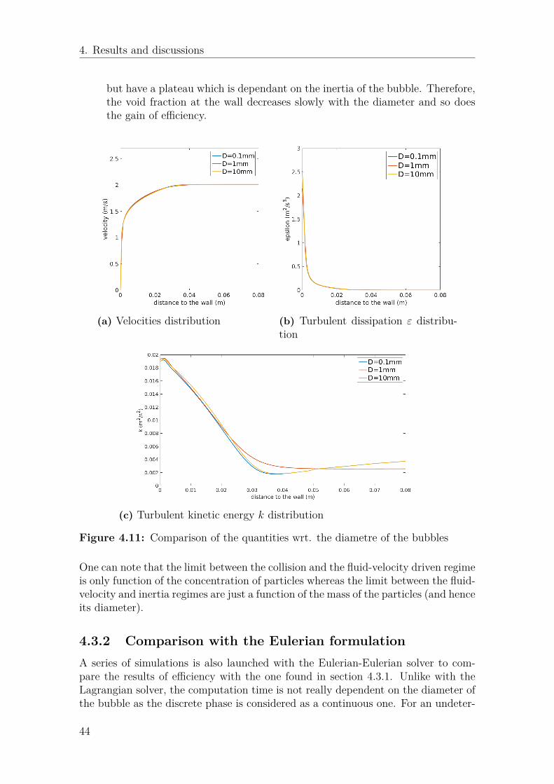
4. Results and discussions
but have a plateau which is dependant on the inertia of the bubble. Therefore,the void fraction at the wall decreases slowly with the diameter and so doesthe gain of efficiency.
(a) Velocities distribution (b) Turbulent dissipation ε distribu-tion
(c) Turbulent kinetic energy k distribution
Figure 4.11: Comparison of the quantities wrt. the diametre of the bubbles
One can note that the limit between the collision and the fluid-velocity driven regimeis only function of the concentration of particles whereas the limit between the fluid-velocity and inertia regimes are just a function of the mass of the particles (and henceits diameter).
4.3.2 Comparison with the Eulerian formulationA series of simulations is also launched with the Eulerian-Eulerian solver to com-pare the results of efficiency with the one found in section 4.3.1. Unlike with theLagrangian solver, the computation time is not really dependent on the diameter ofthe bubble as the discrete phase is considered as a continuous one. For an undeter-
44

4. Results and discussions
mined reason, the solver becomes highly unstable for bubbles with a 3mm diameterso that the simulation for this diameter has not been successfully simulated. Thereason of that remains unknown.
Figure 4.12: Comparison of the skin friction computed by the two solvers
The results are shown in figure 4.12. It can be seen that the results differ greatlyfrom the ones found with the Lagrangian solver. Depending on the diameter, therelative error between the two solvers is between 0 % and 25 %. The reason of thesediscreptancies are studied considering the regimes defined in section 4.3.1 and bycomparing the void fraction distribution.
• For small diameters (the "collision regime"), the results given by the two solversare similar. The comparison of the void fraction distribution shows an identicalshape but the result slightly diverges when close to the wall. This still givea satisfying results as the relative error between the two solvers is lower than5%. Counting that the computation-time is very long for the 2D problem(and hence even more for a 3D problem), it can be really interesting to usethe Eulerian solver for this range of diameter.
• For medium diameter (the "velocity driven regime"), the error is around 15%.The comparison already made in figure 4.6b shows that the height of thepeak is underestimated. This may be improved by adjusting the parametersof the wall-lubrication force. For example, the damping parameter could bedecreased to have a result closer to the Lagrangian framework.
• For big diameter, a strange behaviour appears as there is a sudden jump inthe results at 5mm. The two frameworks give the same results with an errorless than 5% but a closer look at the void fraction distribution and the otherquantities shows that the lateral profiles given by the two solvers are reallydifferent. The similarity may hence be just a coincidence and the Euleriansolver should not be used for this region. This conclusion is understandable,the number of particles for these diameter is so low that having time-averagedcurve takes long with the Lagrangian solver. It is therefore difficult to considerthe air phase as a continuum for such small concentrations.
45

4. Results and discussions
(a) Small diameter (D=0.1mm) (b) Big diameter (D=10mm)
Figure 4.13: Lateral void-fraction for different diameters
4.3.3 Influence of the rate flowThe evolution of the skin friction coefficient with respect to the air rate flow is alsostudied. All the results are presented in percentage as function of the initial air flowQ = 0.00132m3s−1.For 1mm diameter bubbles, the rate flow shows a linear curve for both the methodsbetween 0 % and 100% rate of flow for bubbles. This is shown in figure 4.14. How-ever, the gain of efficiency for higher rates of flow will certainly attain an asymptotewhen it will enter the collision-driven regime.
Figure 4.14: Skin friction coefficient wrt. rate flow for 1mm bubbles
Thus, a study for bubble with 0.2mm is also done to study the behaviour of bubblesthat are in the collision regime. This is shown in figure 4.15. In this regime, theefficiency curve is almost constant: the rate flow does not influence the gain ofefficiency (indeed, more particles would just extend the distribution laterally but
46

4. Results and discussions
would not increase the void fraction at the wall). One can see that for small ratesof flow (from 0 to 10%) a linear curve can be observed which shows that for thisrange of rates of flow, the bubbles are in the "fluid-velocity regime".
Figure 4.15: Skin friction coefficient wrt. rate flow for different diameter of bubbles
47

4. Results and discussions
48

5Conclusion
This master’s thesis gave a first approach on the analysis of a bubble flow undera semi-infinite plate and gave some guidance and recommendations to set-up anefficient method to simulate this flow.
The main result of this study is that an Eulerian-Eulerian solver must be usedcarefully for this type of analysis as it can lead to very different results than fromthe Lagrangian solvers. However, for a very dense concentration of bubbles in theboundary layer – when a Lagrangian simulation becomes very computational in-tensive – the Euler-Euler method can give correct results and save a lot of timecompared to the Lagrangian method. For a less dense solution, the Laplacian Par-ticle Tracking solver should always be preferred.
The Eulerian method is not so accurate because it involves a contradiction aboutthe choice of a correct mesh grid: the mesh’s size must be big enough to incorporatenumerous particles in order to solve average equations but must be small enoughto render the behaviour close to the wall (necessary to compute the shear stress atthe wall). Moreover, the wall lubrication component’s model does not seem suitablefor ship simulations: this model has originally been developed empirically to com-ply with experimental results in a vertical pipe and its generalization to all type ofgeometry is not convincing. A parametric study or even a new formulation of thewall-lubrication force should be developed to better comply with the reality and canallow the use of an Eulerian-Eulerian solver for a wider range of situations.
It has also been shown that the bubbles are spherical and not subjected to coa-lescence and breakage. The turbulence model does not influence so much the resultsand no particular effort should be invested in the choice of it. A first attempt toclassify the behaviour of the air flow depending on the concentration of the particlesand their volume has been developed.
A three-dimensional study should be done as it would facilitate the comparisonwith the experimental results and also lead to a better prediction of the real gain ofefficiency. In particular, numerous bubbles can escape the area below the plate bythe sides and therefore would reduce the expected resistance reduction.
49

5. Conclusion
50

Bibliography
Bhaga, D. and Weber, M. E. (1981). Bubbles in viscous liquids: shapes, wakes andvelocities. Journal of Fluid Mechanics, 105:61–85.
Burns, A. D., Frank, T., Hamill, I., and Shi, J.-M. (2004). The favre averaged dragmodel for turbulent dispersion in eulerian multi-phase flows. In 5th InternationalConference on Multiphase Flow.
Ceccio, S. and Simo, A. M. (2011). Air Lubrication Drag Reduction on Great LakesShips. University of Michigan study for Great Lakes Maritime Institute.
Chen, P., Sanyal, J., and Duduković, M. (2005). Numerical simulation of bubblecolumns flows: effect of different breakup and coalescence closures. ChemicalEngineering Science, 60(4):1085–1101.
Coulaloglou, C. A. and Tavlarides, L. L. (1977). Description of interaction processesin agitated liquid-liquid dispersions. Chemical Engineering Science, 32(11):1289–1297.
Elghobashi, S. (1991). Particle-laden turbulent flows: direct simulation and closuremodels. Applied Scientific Research, 48(3):301–314.
Fan, L.-S. and Tsuchiya, K. (1990). Chapter 2 - single bubble rise characteristics.In Bubble Wake Dynamics in Liquids and Liquid–Solid Suspensions, pages 17–69.Butterworth-Heinemann.
Frank, T., Zwart, P. J., Krepper, E., Prasser, H. M., and Lucas, D. (2008). Val-idation of CFD models for mono and polydisperse air-water two-phase flows inpipes. Nuclear Engineering and Design, 238(3):647–659.
Gharaibah, E. (2008). Entwicklung und Validierung eines Modells polydisperserZweiphasenströmungen unter Berücksichtigung von Koaleszenz und Dispersion.Phd thesis, Universität München.
Hibiki, T. and Ishii, M. (2002). Development of one-group interfacial area transportequation in bubbly flow systems. International Journal of Heat and Mass Transfer,45(11):2351–2372.
Ishii, M., Kim, S., and Uhle, J. (2002). Interfacial area transport equation: modeldevelopment and benchmark experiments. International Journal of Heat and MassTransfer, 45(15):3111–3123.
51

Bibliography
Ishii, M. and Zuber, N. (1979). Drag coefficient and relative velocity in bubbly,droplet or particulate flows. AIChE Journal, 25(5):843–855.
Kawabuchi, M., Mizokami, S., Kodan, Y., Kawakita, C., and Higasa, S. (2011).CFD Predictions of Bubbly Flow around an Energy-saving Ship with MitsubishiAir Lubrication System. Mitsubishi Heavy Industries Technical Review, 48(1).
Kocamustafaogullari, G. and Ishii, M. (1995). Foundation of the interfacial areatransport equation and its closure relations. International Journal of Heat andMass Transfer, 38(3):481–493.
Lahey, R. T. (2005). The simulation of multidimensional multiphase flows. NuclearEngineering and Design, 235(10):1043–1060.
Lamb, H. (1932). Hydrodynamics. Cambridge Univ. Press, 6.ed., repr edition.
Lopez de Bertodano, M. A. (1998). Two fluid model for two-phase turbulent jets.Nuclear Engineering and Design, 179(1):65–74.
Manni, A. (2014). An introduction to twoPhaseEulerFoam with addition of an heatexchange model. Project work for the course in cfd with opensource software,Chalmers University of Technology.
Maritech (2011). The efficacy of air-bubble lubrication for decreasing friction resis-tance. Maritech news, (128).
Michta, E. (2011). Modeling of subcooled nucleate boiling with OpenFoam. Master’sthesis, Royal Institute of Technology, Stockholm.
Nygren, A. (2014). Simulation of bubbly flow in a flat bubble column. Phd thesis,Lund University.
Pang, M. J., Wei, J. J., and Yu, B. (2014). Numerical study on modulation ofmicrobubbles on turbulence frictional drag in a horizontal channel. Ocean Engi-neering, 81:58–68.
Patankar, N. A. and Joseph, D. D. (2001). Lagrangian numerical simulation ofparticulate flows. International Journal of Multiphase Flow, 27(10):1685–1706.
Rusche, H. (2002). Computational fluid dynamics of dispersed two-phase flows athigh-phase fractions. Phd thesis, Imperial College, London.
Sanders, W. C., Winkel, E. S., Dowling, D. R., Perlin, M., and Cecci, S. L. (2006).Bubble friction drag reduction in a high-reynolds-number flat-plate turbulentboundary layer. Journal of Fluid Mechanics, 552:353–380.
Schiller, L. and Naumann, Z. (1935). A Drag Coefficient Correlation. VDI Zeitung,77:318–320.
Snider, D. M. (2001). An incompressible three-dimensional multiphase particle-in-cell model for dense particle flows. Journal of Computational Physics, 170(2):523–549.
52

Bibliography
Tadaki, T. and Maeda, S. (1961). On the shape and velocity of single air bubblesrising in various liquids. Chemical engineering, 25(4):254–264.
Taitel, Y., Bornea, D., and Dukler, A. E. (1980). Modelling flow pattern transitionsfor steady upward gas-liquid flow in vertical tubes. AIChE Journal, 26(3):345–354.
Tomiyama, A., Tamai, H., Zun, I., and Hosokawa, S. (2002). Transverse migration ofsingle bubbles in simple shear flows. Chemical Engineering Science, 57(11):1849–1858.
Tsuchiya, K., Miyahara, T., and Fan, L. S. (1989). Visualization of bubble-wakeinteractions for a stream of bubbles in a two-dimensional liquid-solid fluidizedbed. International Journal of Multiphase Flow, 15(1):35–49.
Vakhrushev, I. A. and Efremov, G. I. (1970). Interpolation formula for computingthe velocities of single gas bubbles in liquids. Chemistry and Technology of Fuelsand Oils, 6(5):376–379.
Vallier, A. (2011). Eulerian and lagrangian cavitation related simulations usingOpenFOAM. Thesis for the degree of licenciate of engineering., Lund University.
Wu, Q., Kim, S., Ishii, M., and Beus, S. G. (1998). One-group interfacial area trans-port in vertical bubbly flow. International Journal of Heat and Mass Transfer,41(8-9):1103–1112.
Yoshida, Y., Takahashi, Y., Kato, H., and Guin, M. M. (1998). Distribution of voidfraction in bubbly flow through a horizontal channel: Bubbly boundary layer flow,2nd report. Journal of Marine Science and Technology, 3(1):30–36.
53

Bibliography
54

ADefinition of the geometry and the
boundary conditions
A.1 Files used by the two solvers
A.1.1 system/blockMeshDict
1 FoamFile2 {3 version 2.0;4 format ascii ;5 class dictionary ;6 object blockMeshDict ;7 }8 convertToMeters 1;9
10 vertices11 (12 (0 0.5 0)13 (2.6 0.5 0)14 (2.6 -0.5 0)15 (0 -0.5 0)16
17 (0 0.5 -0.05)18 (2.6 0.5 -0.05)19 (2.6 -0.5 -0.05)20 (0 -0.5 -0.05)21
22 (0 0.5 -0.20)23 (2.6 0.5 -0.20)24 (2.6 -0.5 -0.20)25 (0 -0.5 -0.20)26 );27
28 blocks29 (30 hex (0 1 2 3 4 5 6 7) (520 1 50)
simpleGrading (1 1 1)31 hex (4 5 6 7 8 9 10 11) (520 1 15)
simpleGrading (1 1 1)32 );33
34 edges
35 (36 );37
38 patches39 (40 patch inlet41 (42 (0 3 7 4)43 )44
45 patch inlet_water46 (47 (4 7 11 8)48 )49
50 patch outlet51 (52 (2 1 5 6)53 (6 5 9 10)54 )55
56 wall walls57 (58 (3 2 1 0)59 )60
61 patch stream62 (63 (11 10 9 8)64 )65 );66
67 mergePatchPairs68 (69 );
I

A. Definition of the geometry and the boundary conditions
A.1.2 0/epsilon.water
1 FoamFile2 {3 version 2.0;4 format ascii ;5 class volScalarField ;6 object epsilon . water ;7 }8
9 dimensions [0 2 -3 0 0 0 0];10
11 internalField uniform 0.027;12
13 boundaryField14 {15 inlet16 {17 type fixedValue ;18 value uniform 0.027;19 }20
21 inlet_water22 {23 type fixedValue ;
24 value uniform 0.027;25 }26
27 outlet28 {29 type inletOutlet ;30 phi phi. water ;31 inletValue $internalField ;32 value $internalField ;33 }34
35 walls36 {37 type
epsilonWallFunction ;38 value $internalField ;39 }40
41 stream42 {43 type zeroGradient ;44 }45 }
A.1.3 0/k.water
1 FoamFile2 {3 version 2.0;4 format ascii ;5 class volScalarField ;6 object k. water ;7 }8
9 dimensions [0 2 -2 0 0 0 0];10
11 internalField uniform 0.01;12
13 boundaryField14 {15 inlet16 {17 type fixedValue ;18 value $internalField ;19 }20
21 inlet_water22 {23 type fixedValue ;
24 value $internalField ;25 }26
27 outlet28 {29 type inletOutlet ;30 phi phi. water ;31 inletValue $internalField ;32 value $internalField ;33 }34
35 walls36 {37 type kqRWallFunction ;38 value $internalField ;39 }40
41 stream42 {43 type zeroGradient ;44 }45 }
A.1.4 0/nut.water
II

A. Definition of the geometry and the boundary conditions
1 FoamFile2 {3 version 2.0;4 format ascii ;5 class volScalarField ;6 object nut. water ;7 }8
9 dimensions [0 2 -1 0 0 0 0];10
11 internalField uniform 1e -8;12
13 boundaryField14 {15 inlet_water16 {17 type calculated ;18 value $internalField ;19 }20
21 inlet22 {
23 type calculated ;24 value $internalField ;25 }26
27 outlet28 {29 type calculated ;30 value $internalField ;31 }32
33 walls34 {35 type nutkWallFunction ;36 value $internalField ;37 }38
39 stream40 {41 type calculated ;42 value $internalField ;43 }44 }
A.1.5 0/U.water
1 FoamFile2 {3 version 2.0;4 format binary ;5 class volVectorField ;6 object U. water ;7 }8 dimensions [0 1 -1 0 0 0 0];9
10 internalField uniform (2 0 0);11
12 boundaryField13 {14 inlet15 {16 type fixedValue ;17 value uniform (2 0 0);18 }19
20 inlet_water21 {22 type fixedValue ;
23 value uniform (2 0 0);24 }25
26 outlet27 {28 type inletOutlet ;29 phi phi. water ;30 inletValue uniform (0 0 0);31 value uniform (0 0 0);32 }33
34 walls35 {36 type fixedValue ;37 value uniform (0 0 0);38 }39
40 stream41 {42 type zeroGradient ;43 }44 }
A.1.6 constant/g
1 FoamFile2 {3 version 2.0;4 format ascii ;
5 classuniformDimensionedVectorField ;
6 location " constant ";7 object g;
III

A. Definition of the geometry and the boundary conditions
8 }9
10 dimensions [0 1 -2 0 0 0 0];11 value (0 0 -9.81);
A.2 Specific files for twoPhaseEulerFoam
A.2.1 0/alpha.air
1 FoamFile2 {3 version 2.0;4 format ascii ;5 class volScalarField ;6 location "0";7 object alpha .air;8 }9
10 dimensions [0 0 0 0 0 0 0];11
12 internalField uniform 0;13
14 boundaryField15 {16 inlet17 {18 type fixedValue ;19 value uniform 0.0132;20 }21
22 inlet_water23 {
24 type fixedValue ;25 value uniform 0;26 }27
28 outlet29 {30 type inletOutlet ;31 phi phi.air;32 inletValue uniform 1;33 value uniform 1;34 }35
36 walls37 {38 type zeroGradient ;39 }40
41 stream42 {43 type zeroGradient ;44 }45 }
A.2.2 0/p
1 FoamFile2 {3 version 2.0;4 format ascii ;5 class volScalarField ;6 object p;7 }8
9 dimensions [1 -1 -2 0 0 0 0];10
11 internalField uniform 1e5;12
13 boundaryField14 {15 inlet16 {17 type calculated ;18 value $internalField ;19 }20
21 inlet_water
22 {23 type calculated ;24 value $internalField ;25 }26
27 outlet28 {29 type calculated ;30 value $internalField ;31 }32
33 walls34 {35 type calculated ;36 value $internalField ;37 }38
39 stream40 {41 type calculated ;42 value $internalField ;
IV

A. Definition of the geometry and the boundary conditions
43 } 44 }
A.2.3 0/p_rgh
1 FoamFile2 {3 version 2.0;4 format ascii ;5 class volScalarField ;6 object p_rgh ;7 }8 dimensions [1 -1 -2 0 0 0 0];9
10 internalField uniform 1e5;11
12 boundaryField13 {14 inlet15 {16 type fixedFluxPressure ;17 value $internalField ;18 }19
20 inlet_water21 {
22 type fixedFluxPressure ;23 value $internalField ;24 }25
26 outlet27 {28 type fixedValue ;29 value uniform 1e5;30 }31
32 walls33 {34 type zeroGradient ;35 }36
37 stream38 {39 type zeroGradient ;40 }41 }
A.2.4 0/U.air
1 FoamFile2 {3 version 2.0;4 format binary ;5 class volVectorField ;6 object U.air;7 }8
9 dimensions [0 1 -1 0 0 0 0];10
11 internalField uniform (2 0 0);12
13 boundaryField14 {15 inlet16 {17 type fixedValue ;18 value uniform (2 0 0);19 }20
21 inlet_water22 {
23 type fixedValue ;24 value uniform (0 0 0);25 }26
27 outlet28 {29 type inletOutlet ;30 value $internalField ;31 inletValue uniform (0 0 0);32 }33
34 walls35 {36 type slip;37 value uniform (0 0 0);
}38
39 stream40 {41 type zeroGradient ;42 }43 }
V

A. Definition of the geometry and the boundary conditions
A.3 Specific files for DPMFoam
A.3.1 0/p
1 FoamFile2 {3 version 2.0;4 format ascii ;5 class volScalarField ;6 object p;7 }8
9 dimensions [0 2 -2 0 0 0 0];10
11 internalField uniform 1e5;12
13 boundaryField14 {15 inlet16 {17 type
fixedFluxPressure ;18 value $internalField ;19 }20
21 inlet_water
22 {23 type
fixedFluxPressure ;24 value $internalField ;25 }26
27 outlet28 {29 type fixedValue ;30 value 1e5;31 }32
33 walls34 {35 type zeroGradient ;36 }37
38 stream39 {40 type zeroGradient ;41 }42 }
VI

BtwoPhaseEulerFoam configuration
files
B.1 constant/phaseProperties
1 FoamFile2 {3 version 2.0;4 format ascii ;5 class dictionary ;6 location " constant ";7 object phaseProperties ;8 }9 phases (air water );
10
11 air12 {13
14 /* Comment to enable IAC equation */15 diameterModel constant ;16 constantCoeffs17 {18 d 1e -3;19 }20
21 residualAlpha 1e -6;22
23 /* Uncomment to enable IAC equation */24
25 // diameterModel IATE;26 // IATECoeffs27 // {28 // dMax 1e -1;29 // dMin 1e -5;30 // residualAlpha 1e -6;31 //32 // sources33 // (34 // wakeEntrainmentCoalescence35 // {36 // Cwe 0.0073;37 // }38 //39 // randomCoalescence40 // {41 // Crc 0.021;
42 // C 3;43 // alphaMax 0.8;44 // }45 //46 // turbulentBreakUp47 // {48 // Cti 0.0945;49 // WeCr 2;50 // }51 // );52 // }53 //54 // residualAlpha 1e -6;55 }56
57 /* Just here for compatibility , not used*/
58 water59 {60 diameterModel constant ;61 constantCoeffs62 {63 d 1e -4;64 }65
66 residualAlpha 1e -6;67 }68
69 blending70 {71 default72 {73 type none;74 continuousPhase water ;75 }76 }77
78 sigma79 (80 (air and water ) 0.0781 );
VII

B. twoPhaseEulerFoam configuration files
82
83 aspectRatio84 (85 (air in water )86 {87 type constant ;88 E0 1.0;89 }90 );91
92 drag93 (94 (air in water )95 {96 type SchillerNaumann ;97 residualRe 1e -3;98 swarmCorrection99 {
100 type none;101 }102 }103 );104
105 virtualMass106 (107 (air in water )108 {109 type
constantCoefficient ;110 Cvm 0.5;111 }112 );113
114 heatTransfer115 (116 (air in water )117 {
118 type RanzMarshall ;119 residualAlpha 1e -4;120 }121 );122
123 lift124 (125 (air in water )126 {127 type
constantCoefficient ;128 Cl 0.5;129 }130 );131
132 wallLubrication133 (134 (air in water )135 {136 type Frank ;137 Cwd 6.8;138 Cwc 10;139 p 1.7;140 }141 );142
143 turbulentDispersion144 (145 (air in water )146 {147 type LopezDeBertodano ;148 Ctd 1;149 }150 );151
152 // Minimum allowable pressure153 pMin 10000;
B.2 constant/thermophysicalProperties.air
1 FoamFile2 {3 version 2.0;4 format ascii ;5 class dictionary ;6 location " constant ";7 object thermophysicalProperties
.air;8 }9
10 thermoType11 {12 type heRhoThermo ;13 mixture pureMixture ;14 transport const ;15 thermo hConst ;16 equationOfState rhoConst ;
17 specie specie ;18 energy
sensibleInternalEnergy ;19 }20
21 mixture22 {23 specie24 {25 nMoles 1;26 molWeight 28.9;27 }28 equationOfState29 {30 rho 1.269;31 }32 thermodynamics
VIII
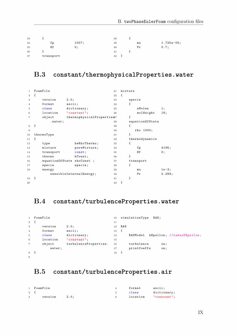
B. twoPhaseEulerFoam configuration files
33 {34 Cp 1007;35 Hf 0;36 }37 transport
38 {39 mu 1.725e -05;40 Pr 0.7;41 }42 }
B.3 constant/thermophysicalProperties.water
1 FoamFile2 {3 version 2.0;4 format ascii ;5 class dictionary ;6 location " constant ";7 object thermophysicalProperties
. water ;8 }9
10 thermoType11 {12 type heRhoThermo ;13 mixture pureMixture ;14 transport const ;15 thermo hConst ;16 equationOfState rhoConst ;17 specie specie ;18 energy
sensibleInternalEnergy ;19 }20
21 mixture22 {23 specie24 {25 nMoles 1;26 molWeight 18;27 }28 equationOfState29 {30 rho 1000;31 }32 thermodynamics33 {34 Cp 4195;35 Hf 0;36 }37 transport38 {39 mu 1e -3;40 Pr 2.289;41 }42 }
B.4 constant/turbulenceProperties.water
1 FoamFile2 {3 version 2.0;4 format ascii ;5 class dictionary ;6 location " constant ";7 object turbulenceProperties .
water ;8 }9
10 simulationType RAS;11
12 RAS13 {14 RASModel kEpsilon ; // LaheyKEpsilon ;15
16 turbulence on;17 printCoeffs on;18 }
B.5 constant/turbulenceProperties.air
1 FoamFile2 {3 version 2.0;
4 format ascii ;5 class dictionary ;6 location " constant ";
IX

B. twoPhaseEulerFoam configuration files
7 object turbulenceProperties .air;
8 }9
10 simulationType RAS;11
12 RAS
13 {14 RASModel continuousGasKEpsilon ; //
continuousGasKEpsilon ;15
16 turbulence off;17 printCoeffs on;18 }
B.6 system/controlDict
1 FoamFile2 {3 version 2.0;4 format ascii ;5 class dictionary ;6 location " system ";7 object controlDict ;8 }9
10 application twoPhaseEulerFoam ;11
12 startFrom startTime ;13
14 startTime 0;15
16 stopAt endTime ;17
18 endTime 5;19
20 deltaT 0.0005;21
22 writeControl runTime ;
23
24 writeInterval 0.1;25
26 purgeWrite 0;27
28 writeFormat ascii ;29
30 writePrecision 6;31
32 writeCompression uncompressed ;33
34 timeFormat general ;35
36 timePrecision 6;37
38 runTimeModifiable yes;39
40 adjustTimeStep yes;41
42 maxCo 0.5;43 maxDeltaT 0.2;
B.7 system/fvSchemes
1 FoamFile2 {3 version 2.0;4 format ascii ;5 class dictionary ;6 location " system ";7 object fvSchemes ;8 }9 ddtSchemes
10 {11 default Euler ;12 }13
14 gradSchemes15 {16 default Gauss linear ;17 }18
19 wallDist
20 {21 method meshWave ;22 nRequired false ;23 }24
25 divSchemes26 {27 default none;28
29 div(phi , alpha .air) Gauss vanLeer ;30 div(phir , alpha .air) Gauss vanLeer ;31
32 "div \( alphaRhoPhi .*,U.*\)" GausslimitedLinearV 1;
33 "div \( phi .*,U.*\)" GausslimitedLinearV 1;
34 div(phi.air , kappai .air) GaussvanLeer ;
35 "div \( alphaRhoPhi .* ,(h|e).*\)" Gauss
X

B. twoPhaseEulerFoam configuration files
limitedLinear 1;36 "div \( alphaRhoPhi .*,K.*\)" Gauss
limitedLinear 1;37 "div \( alphaPhi .*,p\)" Gauss
limitedLinear 1;38 "div \( alphaRhoPhi .* ,(k| epsilon ).*\)"
Gauss limitedLinear 1;39 "div \( phim ,(k| epsilon )m\)" Gauss
limitedLinear 1;40 "div \(\(\(\( alpha .*\* thermo :rho .*\)*
nuEff .*\) \* dev2 \(T\( grad \(U.*\) \)\) \) \)" Gauss linear ;
41 }42
43 laplacianSchemes
44 {45 default Gauss linear
uncorrected ;46 }47
48 interpolationSchemes49 {50 default linear ;51 }52
53 snGradSchemes54 {55 default uncorrected ;56 }
B.8 system/fvSolution
1 FoamFile2 {3 version 2.0;4 format ascii ;5 class dictionary ;6 location " system ";7 object fvSolution ;8 }9
10 solvers11 {12 alpha .air13 {14 nAlphaCorr 1;15 nAlphaSubCycles 2;16 MULESCorr yes;17 nLimiterIter 8;18 }19
20 p_rgh21 {22 solver GAMG;23 smoother DIC;24 nPreSweeps 0;25 nPostSweeps 2;26 nFinestSweeps 2;27 cacheAgglomeration true;28 nCellsInCoarsestLevel 10;29 agglomerator faceAreaPair ;30 mergeLevels 1;31 tolerance 1e -8;32 relTol 0;33 }34
35 p_rghFinal36 {37 $p_rgh ;38 relTol 0;39 }40
41 "(U| kappai ).*"
42 {43 solver smoothSolver ;44 smoother symGaussSeidel ;45 tolerance 1e -5;46 relTol 0;47 minIter 1;48 }49 "(k| epsilon | Theta ).*"50 {51 solver smoothSolver ;52 smoother symGaussSeidel ;53 tolerance 1e -7;54 relTol 0;55 minIter 1;56 }57 }58
59 PIMPLE60 {61 nOuterCorrectors 5;62 nCorrectors 2;63 nNonOrthogonalCorrectors 0;64 residualControl65 {66 p_rgh67 {68 tolerance 1e -3;69 relTol 0;70 }71 }72 }73
74 relaxationFactors75 {76 equations77 {78 "U.*" 0.4;79 " kappai .*" 0.4;80 }81 }
XI

B. twoPhaseEulerFoam configuration files
XII

CDPMFoam configuration files
C.1 constant/kinematicCloudProperties
1 FoamFile2 {3 version 2.0;4 format ascii ;5 class dictionary ;6 location " constant ";7 object particleProperties ;8 }9
10
11 solution12 {13 active true;14 coupled true;15 transient yes;16 cellValueSourceCorrection off;17
18 interpolationSchemes19 {20 rho. water cell;21 U. water cellPoint ;22 mu. water cell;23 curlUcDt cell;24 DUcDt cell;25 }26
27 integrationSchemes28 {29 U Euler ;30 }31
32 sourceTerms33 {34 schemes35 {36 U semiImplicit 1;37 }38 }39 }40
41 constantProperties42 {43 parcelTypeId 1;44
45 rhoMin 1e -15;46 minParcelMass 1e -15;47
48 rho0 1.2;49 youngsModulus 1e -3;50 poissonsRatio 0.5;51
52 constantVolume false ;53
54 alphaMax 0.99;55 }56
57 subModels58 {59 particleForces60 {61 sphereDrag62 {63 alphac alpha . water ;64 }65 gravity ;66 ConstantLift { U U. water ;}67 virtualMass { Cvm 0.5; U U. water ;}68 }69
70 injectionModels71 {72 model173 {74 type
patchInjection ;75 parcelBasisType fixed ;76 patchName inlet ;77 U0 (2 0 0);78 nParticle 1;79 parcelsPerSecond 2521;80 sizeDistribution81 {82 type fixedValue ;83 fixedValueDistribution84 {85 value 1e -3;86 }87 }
XIII

C. DPMFoam configuration files
88 flowRateProfile constant0.00132;
89 massTotal 0;90 SOI 0;91 duration 60;92 }93 }94
95 dispersionModelgradientDispersionRAS ;
96
97 patchInteractionModellocalInteraction ;
98
99 localInteractionCoeffs100 {101 patches102 (103 walls104 {105 type rebound ;106 e 0.97;107 mu 0.09;108 }109
110 " inlet | inlet_water | outlet |stream "
111 {112 type escape ;113 }114 );115 }116
117 StandardWallInteractionCoeffs118 {119 type rebound ;120 e 0.97;121 mu 0.09;122 }123
124 heatTransferModel none;125
126 surfaceFilmModel none;127
128 collisionModel pairCollision ;129
130 pairCollisionCoeffs131 {132 maxInteractionDistance 5e -4;133
134 writeReferredParticleCloud no;135
136 pairModelpairSpringSliderDashpot ;
137
138 pairSpringSliderDashpotCoeffs139 {140 useEquivalentSize no;141 alpha 1;142 b 1;143 mu 0;144 cohesionEnergyDensity 0;145 collisionResolutionSteps 12;146 };147
148 wallModelwallSpringSliderDashpot ;
149
150 wallSpringSliderDashpotCoeffs151 {152 useEquivalentSize no;153 collisionResolutionSteps 12;154 youngsModulus 1e -3;155 poissonsRatio 0.50;156 alpha 1;157 b 1;158 mu 0;159 cohesionEnergyDensity 0;160 };161
162 UName U. water ;163 }164
165 stochasticCollisionModel none;166
167 radiation off;168 }169
170
171 cloudFunctions172 {}
C.2 constant/transportProperties
1 FoamFile2 {3 version 2.0;4 format ascii ;5 class dictionary ;6 location " constant ";7 object transportProperties ;8 }
9
10 continuousPhaseName water ;11
12 rho. water 1000;13
14 transportModel Newtonian ;15 nu 1e -06;
XIV

C. DPMFoam configuration files
C.3 constant/turbulenceProperties.water
1 FoamFile2 {3 version 2.0;4 format ascii ;5 class dictionary ;6 location " constant ";7 object turbulenceProperties .
water ;8 }9
10 simulationType RAS;11
12 RAS13 {14 RASModel kEpsilon ;15
16 turbulence on;17 printCoeffs on;18 }
C.4 system/controlDict
1 FoamFile2 {3 version 2.0;4 format ascii ;5 class dictionary ;6 location " system ";7 object controlDict ;8 }9
10 application DPMFoam ;11
12 startFrom startTime ;13
14 startTime 0;15
16 stopAt endTime ;17
18 endTime 8;19
20 deltaT 2e -3;21
22 writeControl runTime ;
23
24 writeInterval 0.05;25
26 purgeWrite 0;27
28 writeFormat ascii ;29
30 writePrecision 6;31
32 writeCompression uncompressed ;33
34 timeFormat general ;35
36 timePrecision 6;37
38 runTimeModifiable yes;39
40 adjustTimeStep no;41
42 maxCo 0.9;43 maxDeltaT 0.2;
C.5 system/fvSchemes
1 FoamFile2 {3 version 2.0;4 format ascii ;5 class dictionary ;6 object fvSchemes ;7 }8
9 ddtSchemes10 {11 default Euler ;12 }13
14 gradSchemes15 {16 default Gauss linear ;17 }18
19 divSchemes20 {21 default none;22
23 div(alphaPhic ,U. water ) GausslinearUpwindV unlimited ;
24 div(alphaPhic , epsilon . water ) GausslimitedLinear 1;
XV

C. DPMFoam configuration files
25 div(alphaPhic ,k. water ) GausslimitedLinear 1;
26 div ((( alpha . water * nuEff . water )*dev2(T(grad(U. water ))))) Gauss linear;
27 }28
29 laplacianSchemes30 {31 default Gauss linear
corrected ;
32 }33
34 interpolationSchemes35 {36 default linear ;37 }38
39 snGradSchemes40 {41 default corrected ;42 }
C.6 system/fvSolution
1 FoamFile2 {3 version 2.0;4 format ascii ;5 class dictionary ;6 location " system ";7 object fvSolution ;8 }9
10 solvers11 {12 p13 {14 solver GAMG;15 tolerance 1e -06;16 relTol 0.01;17 smoother GaussSeidel ;18 cacheAgglomeration true;19 nCellsInCoarsestLevel 10;20 agglomerator faceAreaPair ;21 mergeLevels 1;22 }23
24 pFinal25 {26 solver GAMG;27 tolerance 1e -06;28 relTol 0;29 smoother GaussSeidel ;30 cacheAgglomeration true;31 nCellsInCoarsestLevel 10;32 agglomerator faceAreaPair ;33 mergeLevels 1;34 }35
36 "(U|k| epsilon ).*"37 {38 solver smoothSolver ;39 smoother symGaussSeidel ;
40 tolerance 1e -05;41 relTol 0.1;42 }43
44 "(U|k| epsilon ).* Final "45 {46 $U;47 tolerance 1e -05;48 relTol 0;49 }50 }51
52 PIMPLE53 {54 pRefPoint (0 0 0);55 pRefValue 0;56 nOuterCorrectors 5;57 nCorrectors 2;58 nNonOrthogonalCorrectors 0;59 residualControl60 {61 p62 {63 tolerance 1e -3;64 relTol 0;65 }66 }67 }68
69 relaxationFactors70 {71 equations72 {73 "U.*" 0.4;74 " kappai .*" 0.4;75
76
77 }78 }
XVI
Related Documents