Hindawi Publishing Corporation Mathematical Problems in Engineering Volume 2010, Article ID 879519, 23 pages doi:10.1155/2010/879519 Research Article Numerical Investigation of Aeroelastic Mode Distribution for Aircraft Wing Model in Subsonic Air Flow Marianna A. Shubov, Stephen Wineberg, and Robert Holt Department of Mathematics and Statistics, University of New Hampshire, Durham, NH 03824, USA Correspondence should be addressed to Marianna A. Shubov, [email protected] Received 31 July 2009; Accepted 30 November 2009 Academic Editor: Jos´ e Balthazar Copyright q 2010 Marianna A. Shubov et al. This is an open access article distributed under the Creative Commons Attribution License, which permits unrestricted use, distribution, and reproduction in any medium, provided the original work is properly cited. In this paper, the numerical results on two problems originated in aircraft wing modeling have been presented. The first problem is concerned with the approximation to the set of the aeroelastic modes, which are the eigenvalues of a certain boundary-value problem. The affirmative answer is given to the following question: can the leading asymptotical terms in the analytical formulas be used as reasonably accurate description of the aeroelastic modes? The positive answer means that these leading terms can be used by engineers for practical calculations. The second problem is concerned with the flutter phenomena in aircraft wings in a subsonic, incompressible, inviscid air flow. It has been shown numerically that there exists a pair of the aeroelastic modes whose behavior depends on a speed of an air flow. Namely, when the speed increases, the distance between the modes tends to zero, and at some speed that can be treated as the flutter speed these two modes merge into one double mode. 1. Introduction and Formulation of Problem The main goal of this paper is to present the numerical results for two problems arising in aircraft wing modeling. The first one is related to the numerical approximation of the discrete spectrum of a certain matrix differential operator that represents the structural part of an aircraft wing model in a subsonic incompressible inviscid air flow. More precisely, it is shown that the asymptotic approximation for the set of aeroelastic modes has a very regular structure, that is, there are two distinct branches which are called the β-branch and the δ-branch see formulas 2.2, 2.3. Each branch is described by leading asymptotical terms and remainder terms. An affirmative answer is given to the following question: can the leading asymptotical terms be used as a reasonably accurate description of the aeroelastic modes? The question can be rephrased as: if one discretizes the main matrix differential

Welcome message from author
This document is posted to help you gain knowledge. Please leave a comment to let me know what you think about it! Share it to your friends and learn new things together.
Transcript
Hindawi Publishing CorporationMathematical Problems in EngineeringVolume 2010, Article ID 879519, 23 pagesdoi:10.1155/2010/879519
Research ArticleNumerical Investigation of Aeroelastic ModeDistribution for Aircraft Wing Model inSubsonic Air Flow
Marianna A. Shubov, Stephen Wineberg, and Robert Holt
Department of Mathematics and Statistics, University of New Hampshire, Durham, NH 03824, USA
Correspondence should be addressed to Marianna A. Shubov, [email protected]
Received 31 July 2009; Accepted 30 November 2009
Academic Editor: Jose Balthazar
Copyright q 2010 Marianna A. Shubov et al. This is an open access article distributed underthe Creative Commons Attribution License, which permits unrestricted use, distribution, andreproduction in any medium, provided the original work is properly cited.
In this paper, the numerical results on two problems originated in aircraft wing modeling havebeen presented. The first problem is concerned with the approximation to the set of the aeroelasticmodes, which are the eigenvalues of a certain boundary-value problem. The affirmative answeris given to the following question: can the leading asymptotical terms in the analytical formulasbe used as reasonably accurate description of the aeroelastic modes? The positive answer meansthat these leading terms can be used by engineers for practical calculations. The second problem isconcerned with the flutter phenomena in aircraft wings in a subsonic, incompressible, inviscid airflow. It has been shown numerically that there exists a pair of the aeroelastic modes whose behaviordepends on a speed of an air flow. Namely, when the speed increases, the distance between themodes tends to zero, and at some speed that can be treated as the flutter speed these two modesmerge into one double mode.
1. Introduction and Formulation of Problem
The main goal of this paper is to present the numerical results for two problems arisingin aircraft wing modeling. The first one is related to the numerical approximation of thediscrete spectrum of a certain matrix differential operator that represents the structural partof an aircraft wing model in a subsonic incompressible inviscid air flow. More precisely, itis shown that the asymptotic approximation for the set of aeroelastic modes has a veryregular structure, that is, there are two distinct branches which are called the β-branch andthe δ-branch (see formulas (2.2), (2.3)). Each branch is described by leading asymptoticalterms and remainder terms. An affirmative answer is given to the following question: can theleading asymptotical terms be used as a reasonably accurate description of the aeroelasticmodes? The question can be rephrased as: if one discretizes the main matrix differential
2 Mathematical Problems in Engineering
operator with spectral methods, can the spectrum of the discretized finite-dimensionaloperator be described by the leading asymptotical terms of the continuous operator? Theanswer is affirmative, and one can see almost perfect spectral branches for the finite-dimensional approximation (see Figure 2).
The second problem is related to the entire model involving both the structural andaerodynamical parts. In the second problem, the authors provide a numerical justificationof a certain fact well-known in the aircraft engineering community. Namely, it is shown thatthere exists a pair of the aeroelastic modes whose behavior depends on a speed of an airflow in the following way: the distance between these aeroelastic modes tends to zero withincreasing speed. At some speed that can be treated as “the flutter speed”, the two modesmerge in one double mode. If a speed continues to increase, the double aeroelastic modesplits up into two simple modes that are moving apart. Such a dynamics clearly indicatesthat there exists a specific speed (“the flutter speed”) that causes an appearance of a doubleaeroelastic mode leading to a flutter instability. In this study, the authors deal with a linearwing model, which is obviously a significant simplification of a realistic situation. In a moreprecise setting, when the speed is near what is called “the flutter speed”, one should usea nonlinear wing model, which results in limit cycle oscillations rather than flutter. One ofthe important conclusions of this investigation is that even though the model studied in thepaper is linear, it is capable of capturing the flutter instability, which is definitely supportedby numerical simulations. Before the numerical analysis results, a mathematical statement ofthe problem and a description of those analytical results that are relevant to the numericalanalysis will be given.
An ultimate goal of an aircraft wing modeling is to find an approach to flutter control.Flutter is a structural dynamical instability, which consists of violent vibrations of the solidstructure with rapidly increasing amplitude [1, 2]. The physical reason for this phenomenonis that under special conditions, the energy of air flow is rapidly absorbed by the structure andtransformed into the energy of mechanical vibrations. In engineering practice, flutter mustbe avoided either by design of the structure or by introducing control mechanism capableto suppress harmful vibrations. Flutter is an inherent feature of fluid-structure interactionand, thus, it cannot be eliminated completely. However, the critical conditions for the flutteronset can be shifted to the safe range of the operating parameters. This is exactly the goal fordesigning flutter control mechanisms.
Flutter is an in-flight event, which happens beyond some speed-altitude combinations.High-speed aircrafts are most susceptible for flutter although no speed regime is trulyimmune from flutter. Flutter instabilities occur in a variety of different engineering and evenbiomedical situations. Namely in aeronautic engineering, flutter of helicopter, propeller, andturbine blades is a serious problem. It also affects electric transmission lines, high-speed harddisk drives, and long-spanned suspension bridges. Flutter of cardiac tissue and blood vesselwalls is of a special concern to medical practitioners.
At the present moment, there exist only a few models of fluid-structure interactioninvolving flutter development, for which precise mathematical formulations are available.The authors’ main objects of interest are analytical and numerical results on such models,which can be used, in particular, for flutter explanation. It is certainly important for designingflutter control mechanisms.
Ideally, a complete picture of a fluid-structure interaction should be described bya system of partial differential equations, a system which contains both the equationsgoverning the vibrations of an elastic structure and the hydrodynamic equations governingthe motion of gas or fluid flow. The system of equations of motion should be supplied

Mathematical Problems in Engineering 3
Trailing edge
Center of gravityBa
x
L
B
0
−B
−→u
Leading edge
Span: L Halfcord: B
Figure 1: Wing structure beam model.
with appropriate boundary and initial conditions. The structural and hydrodynamic partsof the system must be coupled in the following sense. The hydrodynamic equations definea pressure distribution on the elastic structure. This pressure distribution in turn defines theso-called aerodynamic loads, which appear as forcing terms in structural equations. On theother hand, the parameters of the elastic structure enter the boundary conditions for thehydrodynamic equations.
In the present paper it is assumed that the model describes a wing of high-aspect ratio(i.e., the length of a wing is much greater than its width, though both quantities are finite)in a subsonic, inviscid, incompressible air flow. The hydrodynamic equations have been solvedexplicitly and aerodynamic loads are represented as forcing terms in the structural equationsas time convolution-type integrals with complicated kernels. Thus, the model is describedby a system of integro-differential equations. Analytical results on this model include thefollowing. The system of equations of motion is treated as a single evolution-convolutionequation in the Hilbert state space of the model. (The integral convolution part of thisequation vanishes if a speed of an air stream is zero, and the equations of motion describethe so-called ground vibrations.) After applying a Laplace transformation with respect tothe time variable to both sides of the evolution equation, one obtains a matrix differentialequation involving the complex parameter λ. For this new equation, the following resultshave been shown.
(a) The representation of the solution of the original initial boundary-value problem inthe frequency domain has been given in terms of the generalized resolvent, which is an analyticoperator-valued function of the spectral parameter λ. The aeroelastic modes are defined asthe poles of the generalized resolvent; the corresponding mode shapes are defined in termsof the residues at these poles [3–5].
(b) Explicit asymptotic formulas for the aeroelastic modes have been derived [4, 6].(To the best of the authors’ knowledge, these are the first such formulas in the literatureon aeroelasticity.) The entire set of aeroelastic modes splits into two branches, which areasymptotically close to the eigenvalues of the structural part of the system [3, 5, 7].
(c) It has been shown that the set of the mode shapes forms a nonorthogonal basis(Riesz basis) of the state space of the system. (The set of the generalized eigenvectors of thestructural part of the system has a similar property [4, 8].)
1.1. Statement of Problem. Operator Setting in Energy Space
The so-called “Goland model” [1, 6, 9] is considered, that is, the simplest structural model—a uniform rectangular beam (Figure 1) with two types of motion, plunge and pitch. To
4 Mathematical Problems in Engineering
formulate a mathematical model, the following dynamical variables are introduced [3, 4, 9,10]:
X(x, t) =
(h(x, t)
α(x, t)
), −L ≤ x ≤ 0, t ≥ 0, (1.1)
where h(x, t) is the bending, α(x, t) is the torsion angle, and x is the span variable. The modelcan be described by the following linear system:
(Ms −Ma)X(x, t) + (Ds − uDa)X(x, t) +(Ks − u2Ka
)X(x, t) =
[f1(x, t)
f2(x, t)
], (1.2)
where the “overdot” denotes the differentiation with respect to time t. The subscripts “s” and“a” are use to distinguish the structural and aerodynamical parameters, respectively. All 2×2matrices in (1.2) are given by the following formulas:
Ms =
[m S
S I
], Ma =
(−πρ
)⎡⎢⎣
1 −a
−a(a2 +
18
)⎤⎥⎦, Ds =
[0 0
0 0
], (1.3)
where m is the density of the flexible structure, S is the mass moment, I is the moment ofinertia, ρ is the density of air, a is the linear parameter of the structure, and −1 ≤ a ≤ 1 (a isa relative distance between the elastic axis of a model wing and its line of center of gravity).Even though in the current paper the matrixDs has only trivial entries, it is preferable to keepit in (1.2) since the problem with a nontrivial structural damping Ds will be studied in theauthors’ forthcoming paper:
Da =(−πρ
)[ 0 1
−1 0
], Ks =
⎡⎢⎢⎣E∂4
∂x40
0 −G ∂2
∂x2
⎤⎥⎥⎦, Ka =
(−πρ
) [0 0
0 −1
], (1.4)
where E is the bending stiffness, and G is the torsion stiffness. The parameter u in (1.2)denotes the stream speed. The right hand side of system (1.2) can be represented as

Mathematical Problems in Engineering 5
the following system of two convolution-type integral operations:
f1(x, t) = −2πρ∫ t
0
[uC2(t − σ) − C3(t − σ)
]g(x, σ)dσ ≡
∫ t0C1(t − σ)g(x, σ)dσ, (1.5)
f2(x, t) = −2πρ∫ t
0
[12C1(t − σ) − auC2(t − σ) + aC3(t − σ)
+ uC4(t − σ) +12C5(t − σ)
]g(x, σ)dσ ≡
∫ t0C2(t − σ)g(x, σ)dσ,
(1.6)
g(x, t) = uα(x, t) + h(x, t) +(
12− a)α(x, t). (1.7)
Explicit formulas for the aerodynamical functions Ci, i = 1, . . . , 5, can be found in [11]. Itis known that the self-straining control actuator action can be modeled by the followingboundary conditions [5, 9, 12–14]:
Eh′′(0, t) + βh′(0, t) = 0, h′′′(0, t) = 0, Gα′(0, t) + δα(0, t) = 0, β, δ ∈ C+ ∪ {∞},
(1.8)
where C+ is the closed right half-plane. The boundary conditions at x = −L are
h(−L, t) = h′(−L, t) = α(−L, t) = 0. (1.9)
In (1.8) and (1.9) and below, the prime designates derivative with respect to x. The initialstate of the system is given as follows:
h(x, 0) = h0(x), h(x, 0) = h1(x), α(x, 0) = α0(x), α(x, 0) = α1(x). (1.10)
The solution of the problem given by (1.2) and conditions (1.8)–(1.10) are given in the energyspace H. It is assumed that the parameters satisfy the following two conditions:
det
[m S
S I
]> 0, 0 < u ≤
√2G
L√πρ
. (1.11)
The second condition in (1.11) means that the flow speed must be below the “divergence” orstatic aeroelastic instability speed. The state space H, which is a Hilbert space, is describedas the set of 4-component vector-valued functions Ψ = (h, h, α, α)T ≡ (ψ0, ψ1, ψ2, ψ3)
T (“T”stands for transposition) obtained as a closure of smooth functions satisfying the boundaryconditions
ψ0(−L) = ψ ′0(−L) = ψ2(−L) = 0 (1.12)

6 Mathematical Problems in Engineering
in the following energy norm, which is well-defined under conditions (1.11):
‖Ψ‖2H =
12
∫0
−L
[E∣∣ψ ′′
0(x)∣∣2 +G∣∣ψ ′
2(x)∣∣2 + m∣∣ψ1(x)
∣∣2 + I∣∣ψ3(x)∣∣2
+ S(ψ3(x)ψ1(x) + ψ3(x)ψ1(x)
)− πρu2∣∣ψ2(x)
∣∣2]dx,(1.13)
where the following notations have been used:
m = m + πρ, S = S − aπρ, I = I + πρ(a2 +
18
), Δ = mI − S2. (1.14)
The initial-boundary value problem defined by (1.2) and conditions (1.8)–(1.10) can berepresented in the following form
Ψ = iLβδΨ + FΨ, Ψ =(ψ0, ψ1, ψ2, ψ3
)T, Ψ|t=0 = Ψ0. (1.15)
Lβδ is a matrix differential operator in H given by the following expression:
Lβδ = −i
⎡⎢⎢⎢⎢⎢⎢⎢⎢⎢⎢⎢⎢⎢⎣
0 1 0 0
−EIΔ
d4
dx4−πρuS
Δ− SΔ
(Gd2
dx2+ πρu2
)−πρuI
Δ
0 0 0 1
ES
Δd4
dx4
πρum
Δm
Δ
(Gd2
dx2+ πρu2
)πρuS
Δ
⎤⎥⎥⎥⎥⎥⎥⎥⎥⎥⎥⎥⎥⎥⎦
(1.16)
defined on the domain
D(Lβδ
)={Ψ ∈ H : ψ0 ∈ H4(−L, 0), ψ1 ∈ H2(−L, 0), ψ2 ∈ H2(−L, 0),
ψ3 ∈ H1(−L, 0); ψ1(−L) = ψ ′1(−L) = ψ3(−L) = 0; ψ ′′′
0 (0) = 0;
Eψ ′′0(0)+βψ
′1(0) = 0, Gψ ′
2(0) + δψ3(0) = 0}.
(1.17)
F is a linear integral operator in H given by the formula
F =1Δ
⎡⎢⎢⎢⎢⎢⎢⎣
1 0 0 0
0[I(C1∗)− S(C2∗)]
0 0
0 0 1 0
0 0 0[−S(C1∗)+ m(C2∗)]
⎤⎥⎥⎥⎥⎥⎥⎦
⎡⎢⎢⎢⎢⎢⎢⎢⎢⎣
0 0 0 0
0 1 u
(12− a)
0 0 0 0
0 1 u
(12− a)
⎤⎥⎥⎥⎥⎥⎥⎥⎥⎦. (1.18)
Mathematical Problems in Engineering 7
In (1.18), the star “∗” stands for the convolution operation and the kernels C1 and C2 aredefined in (1.5), and (1.6).
Remark 1.1. It is important to emphasize that (1.15) is not an evolution equation. It does nothave a dynamics generator and does not define any semigroup in the standard sense. Byapplying the Laplace transformation to both sides of (1.15), one obtains the following Laplacetransform representation of the solution:
Ψ(λ) = −(λI − iLβδ − λF(λ)
)−1(I − F(λ)
)Ψ0. (1.19)
To find the solution in the space-time domain, one has to “calculate” the inverse Laplacetransform of Ψ by contour integration in the complex λ-plane. In this connection, theproperties of the “generalized resolvent operator”
R(λ) =(λI − iLβδ − λF(λ)
)−1(1.20)
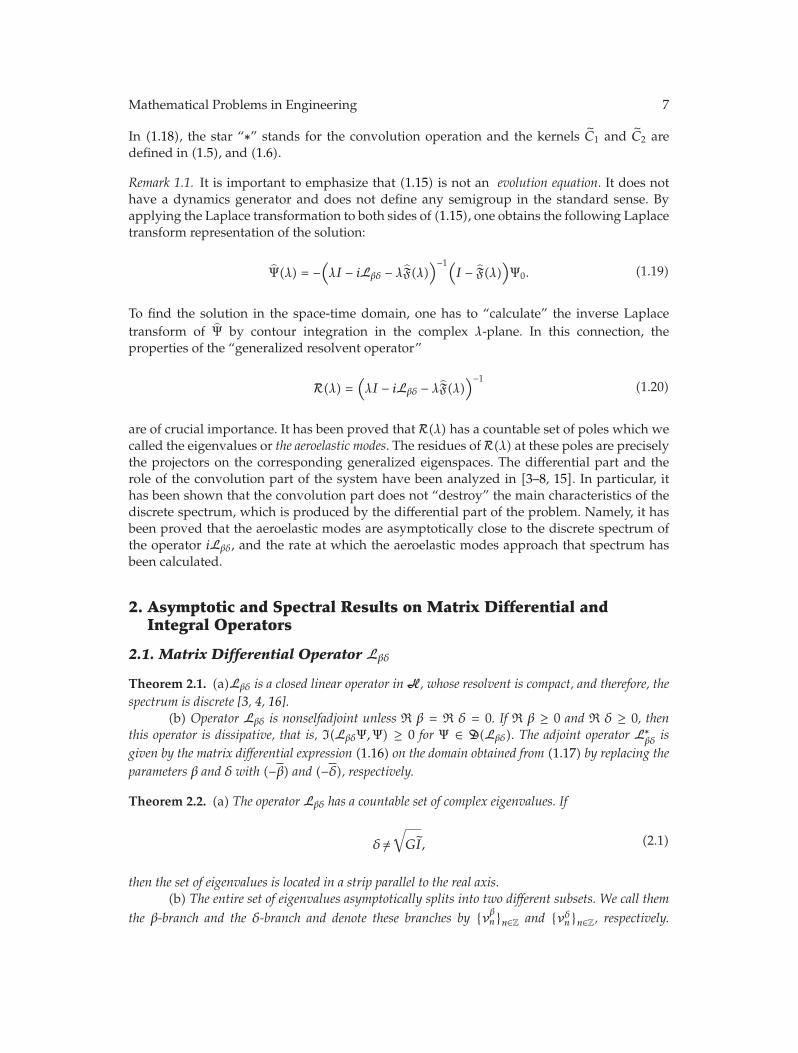
are of crucial importance. It has been proved that R(λ) has a countable set of poles which wecalled the eigenvalues or the aeroelastic modes. The residues of R(λ) at these poles are preciselythe projectors on the corresponding generalized eigenspaces. The differential part and therole of the convolution part of the system have been analyzed in [3–8, 15]. In particular, ithas been shown that the convolution part does not “destroy” the main characteristics of thediscrete spectrum, which is produced by the differential part of the problem. Namely, it hasbeen proved that the aeroelastic modes are asymptotically close to the discrete spectrum ofthe operator iLβδ, and the rate at which the aeroelastic modes approach that spectrum hasbeen calculated.
2. Asymptotic and Spectral Results on Matrix Differential andIntegral Operators
2.1. Matrix Differential Operator Lβδ
Theorem 2.1. (a)Lβδ is a closed linear operator in H, whose resolvent is compact, and therefore, thespectrum is discrete [3, 4, 16].
(b) Operator Lβδ is nonselfadjoint unless R β = R δ = 0. If R β ≥ 0 and R δ ≥ 0, thenthis operator is dissipative, that is, I(LβδΨ,Ψ) ≥ 0 for Ψ ∈ D(Lβδ). The adjoint operator L∗
βδis
given by the matrix differential expression (1.16) on the domain obtained from (1.17) by replacing theparameters β and δ with (−β) and (−δ), respectively.
Theorem 2.2. (a) The operator Lβδ has a countable set of complex eigenvalues. If
δ /=√GI, (2.1)
then the set of eigenvalues is located in a strip parallel to the real axis.(b) The entire set of eigenvalues asymptotically splits into two different subsets. We call them
the β-branch and the δ-branch and denote these branches by {νβn}n∈Zand {νδn}n∈Z
, respectively.
8 Mathematical Problems in Engineering
If R β ≥ 0 and R δ > 0, then each branch is asymptotically close to its own horizontal line inthe closed upper half-plane. If R β > 0 and R δ = 0, then both horizontal lines coincide with the realaxis. If R β = R δ = 0, then the operator Lβδ is selfadjoint and, thus, its spectrum is real.
(c) The following asymptotics are valid for the β-branch of the spectrum as |n| → ∞:
νβn =(sgn n
)(π2
L2
)√EI
Δ
(|n| − 1
4
)2
+ κn(ω), ω = |δ|−1 +∣∣β∣∣−1
, (2.2)
with Δ being defined in (1.14). A complex-valued sequence {κn} is bounded above in the followingsense: supn∈Z
{|κn(ω)|} = C(ω), C(ω) → 0 as ω → 0.(d) The following asymptotics are valid for the δ-branch of the spectrum:
νδn =πn
L
√I/G
+i
2L√I/G
lnδ +√GI
δ −√GI
+O(|n|−1/2
), |n| −→ ∞. (2.3)
In (2.3), “ln” means the principal value of the logarithm. If β and δ stay away from zero, that is,|β| ≥ β0 > 0 and |δ| ≥ δ0 > 0, then the estimate O(|n|−1/2) in (2.3) is uniform with respect to bothparameters.
(e) There may be only a finite number of multiple eigenvalues of a finite multiplicity each.Therefore, only a finite number of the associate vectors may exist.
The theorem below deals with the Riesz basis property of the generalized eigenvectorsof the structural operator Lβδ. The Riesz basis is a mild modification of an orthonormal basis,namely a linear isomorphism of an orthonormal basis.
Theorem 2.3. The set of generalized eigenvectors of the operatorLβδ forms a Riesz basis in the energyspaceH.
The next statement deals with the asymptotic distribution of the aeroelastic modes[4, 7, 15].
Theorem 2.4. (a) The set of the aeroelastic modes (which are the poles of the generalized resolventoperator) is countable and does not have accumulation points on the complex plane C. There mightbe only a finite number of multiple poles of a finite multiplicity each. There exists a sufficiently largeR > 0 such that all aeroelastic modes, whose distance from the origin is greater than R, are simple polesof the generalized resolvent. The value of R depends on the speed u of an airstream, that is, R = R(u).
(b) The set of the aeroelastic modes splits asymptotically into two series, which we call theβ-branch and the δ-branch. Asymptotical distribution of the β-and the δ-branches of the aeroelasticmodes can be obtained from asymptotical distribution of the spectrum of the operator Lβδ. Namely if
{λβn}n∈Zis the β-branch of the aeroelastic modes, then λβn = iλβn and the asymptotics of the set {λβn}n∈Z
is given by the right-hand side of formula (2.2). Similarly, if {λδn = iλδn}n∈Zis the δ-branch of the
aeroelastic modes, then the asymptotical distribution of the set {λδn}n∈Zis given by the right-hand side
of formula (2.3).
Mathematical Problems in Engineering 9
2.2. Structure and Properties of the Matrix Integral Operator
Important information on the Laplace transform of the convolution-type matrix integraloperator (1.18) is collected below.
Lemma 2.5. Let F be the Laplace transform of the kernel of matrix integral operator (1.18). Thefollowing formula is valid for F :
F(λ) =
⎡⎢⎢⎢⎢⎢⎢⎢⎢⎢⎢⎢⎣
0 0 0 0
0 L(λ) uL(
12− a)L(λ)
0 0 0 0
0 N(λ) uN(λ)(
12− a)N(λ)
⎤⎥⎥⎥⎥⎥⎥⎥⎥⎥⎥⎥⎦, (2.4)
where
L(λ) = −2πρΔ
u
λ
{− S
2+[I +(a +
12
)S
]T
(λ
u
)},
N(λ) = −2πρΔ
u
λ
{m
2−[S +(a +
12
)m
]T
(λ
u
)},
(2.5)
and T is the Theodorsen function defined by the formula
T(z) =K1(z)
K0(z) +K1(z); (2.6)
K0 and K1 are the modified Bessel functions [17].
2.3. Properties of the Theodorsen Function
The Theodorsen function is a bounded analytic function on the complex plane with thebranch-cut along the negative real semi-axis. As |z| → ∞, the following asymptoticrepresentation holds:
T(z) =12+O(
11 + |z|
), as |z| −→ ∞. (2.7)
10 Mathematical Problems in Engineering
Taking into account that z = λ/u, one can write λF(λ) as the following sum: λF(λ) = M+N(λ),where the matrix M is defined by the formula
M =
⎡⎢⎢⎢⎢⎢⎢⎢⎢⎢⎣
0 0 0 0
0 A uA
(12− a)A
0 0 0 0
0 B uB
(12− a)B
⎤⎥⎥⎥⎥⎥⎥⎥⎥⎥⎦
(2.8)
with A and B being given by
A = −πρuΔ−1[I +(a − 1
2
)S
], B = πρuΔ−1
[S +(a − 1
2
)m
]. (2.9)
The matrix-valued function N(λ) is defined by the formula
N(λ) =
⎡⎢⎢⎢⎢⎢⎢⎢⎢⎢⎣
0 0 0 0
0 A1(λ) uA1(λ)(
12− a)A1(λ)
0 0 0 0
0 B1(λ) uB1(λ)(
12− a)B1(λ)
⎤⎥⎥⎥⎥⎥⎥⎥⎥⎥⎦, (2.10)
where A1(λ) = −2πρuΔ−1(T(λ/u) − 1/2)[I + (a + 1/2)S], and B1(λ) = 2πρuΔ−1(T(λ/u) −1/2)[S+(a+1/2)m]. For each λ, N(λ) is a bounded operator in H with the following estimatefor its norm:
‖N‖H ≤ C(1 + |λ|)−1, (2.11)
where C is an absolute constant the precise value of which is immaterial for us. Therefore, thegeneralized resolvent (1.20) can be written in the form
R(λ) = S−1(λ), where S(λ) = λI − iLβδ − M − N(λ). (2.12)
Theorem 2.6. M is a bounded linear operator inH. The operator Kβδ defined by
Kβδ = Lβδ − i M (2.13)
is an unbounded nonselfadjoint operator in H with compact resolvent. The spectral asymptotics ofKβδ coincide with the spectral asymptotics of Lβδ (see Theorem 2.2). In contrast to Lβδ, the operatorKβδ is not dissipative for any boundary control gains. However,Kβδ is also a Riesz spectral operator,that is, the set of its generalized eigenvectors forms a Riesz basis ofH.

Mathematical Problems in Engineering 11
3. Numerical Results for Two-Branch Discrete Spectrum ofOperator Lβδ
The first question is related to the accuracy of the asymptotic approximations of theeigenvalues of the operator Lβδ. By their nature, asymptotic formulas (2.2) and (2.3) shouldbe understood in the following way.
Formula (2.2) for the β-branch eigenvalues means that there exist a positive numberN1 and a small constant 0 < ε 1 such that for all |n| ≥ N1, the β-branch eigenvalues (2.2)satisfy the estimate
∣∣∣∣∣∣νβn −(sgnn
)(π2
L2
)√EI
Δ
(|n| − 1
4
)2∣∣∣∣∣∣ ≤ ε. (3.1)
In other words, for |n| ≥ N1, all eigenvalues {νβn} are located in the ε-vicinity of the
points {◦νβ
n}, given by the leading asymtotical term of (2.2). Obviously, ε can be chosen assmall as desired by manipulating the control parameters β and δ.
Formula (2.3) for the δ-branch means that there exists N2 > 0 and ε > 0 such that forall |n| ≥N2 the δ-branch eigenvalues satisfy the estimate
∣∣∣∣∣∣∣νδn −
πn
L
√I/G
− ı
2L√I/G
lnδ +√GI
δ −√GI
∣∣∣∣∣∣∣ ≤ε√|n|. (3.2)
This formula means that for |n| ≥ N2 each eigenvalue νδn is located in a small circle of radius
that tends to zero at the rate |n|−1/2 and is centered at the points {◦νβ
n}; each center coincideswith the leading asymptotical term from (2.3).
Regarding this description, the following important question holds: from whichnumbers N1 and N2 can the eigenvalues be approximated by the leading asymptotical termswith acceptable accuracy? In other words, can one claim that asymptotical formulas (2.2) and(2.3) are valuable for practitioners or are they just important analytical results of the spectralanalysis?
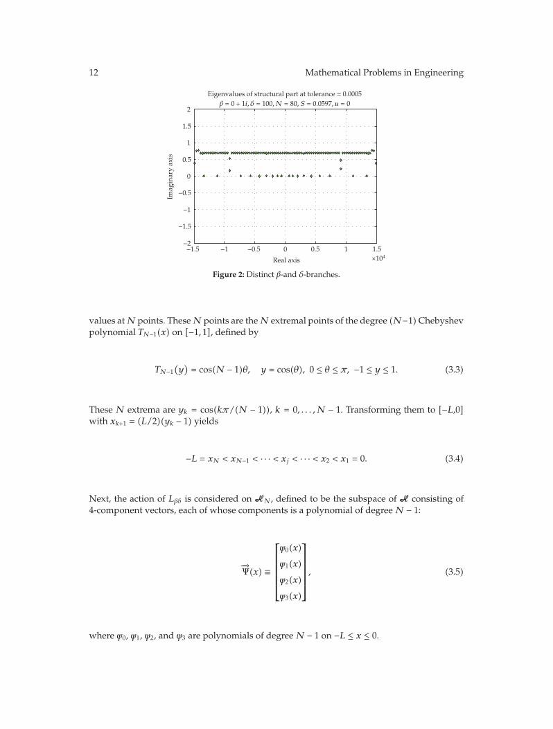
As is well known, from practical applications only the first dozen of the lowest eigen-frequencies are important for engineers. The results of numerical simulations below showthat the asymtotical formulas are indeed quite accurate, that is, if one places on the complexplane the numerically produced β-branch and δ-branch eigenvalues, then the theoreticallypredicted branches can be seen practically immediately (see Figure 2).
Figure 2 means that the leading terms from asymptotics (2.2) and (2.3) can be used bypractitioners as good approximations for the eigenvalues.
The numerical procedure which is quite nontrivial, is briefly outlined below. Thenumerical approximation is based on Chebyshev polynomials. First, a finite-dimensionalapproximation for the main differential operator Lβδ, (denoted by Lβδ) is described. Let HN
be an N-dimensional subspace of polynomials of degree (N − 1); obviously HN ⊂ H, whereH is the main Hilbert space with norm (1.13). Each polynomial is uniquely determined by its
12 Mathematical Problems in Engineering
Eigenvalues of structural part at tolerance = 0.0005β = 0 + 1i, δ = 100,N = 80, S = 0.0597, u = 0
×1041.510.50−0.5−1−1.5
Real axis
−2
−1.5
−1
−0.5
0
0.5
1
1.5
2
Imag
inar
yax
is
Figure 2: Distinct β-and δ-branches.
values atN points. TheseN points are theN extremal points of the degree (N−1) Chebyshevpolynomial TN−1(x) on [−1, 1], defined by
TN−1(y)= cos(N − 1)θ, y = cos(θ), 0 ≤ θ ≤ π, −1 ≤ y ≤ 1. (3.3)
These N extrema are yk = cos(kπ/(N − 1)), k = 0, . . . ,N − 1. Transforming them to [−L,0]with xk+1 = (L/2)(yk − 1) yields
−L = xN < xN−1 < · · · < xj < · · · < x2 < x1 = 0. (3.4)
Next, the action of Lβδ is considered on HN , defined to be the subspace of H consisting of4-component vectors, each of whose components is a polynomial of degree N − 1:
−→Ψ(x) ≡
⎡⎢⎢⎢⎢⎢⎣
ψ0(x)
ψ1(x)
ψ2(x)
ψ3(x)
⎤⎥⎥⎥⎥⎥⎦, (3.5)
where ψ0, ψ1, ψ2, and ψ3 are polynomials of degree N − 1 on −L ≤ x ≤ 0.
Mathematical Problems in Engineering 13
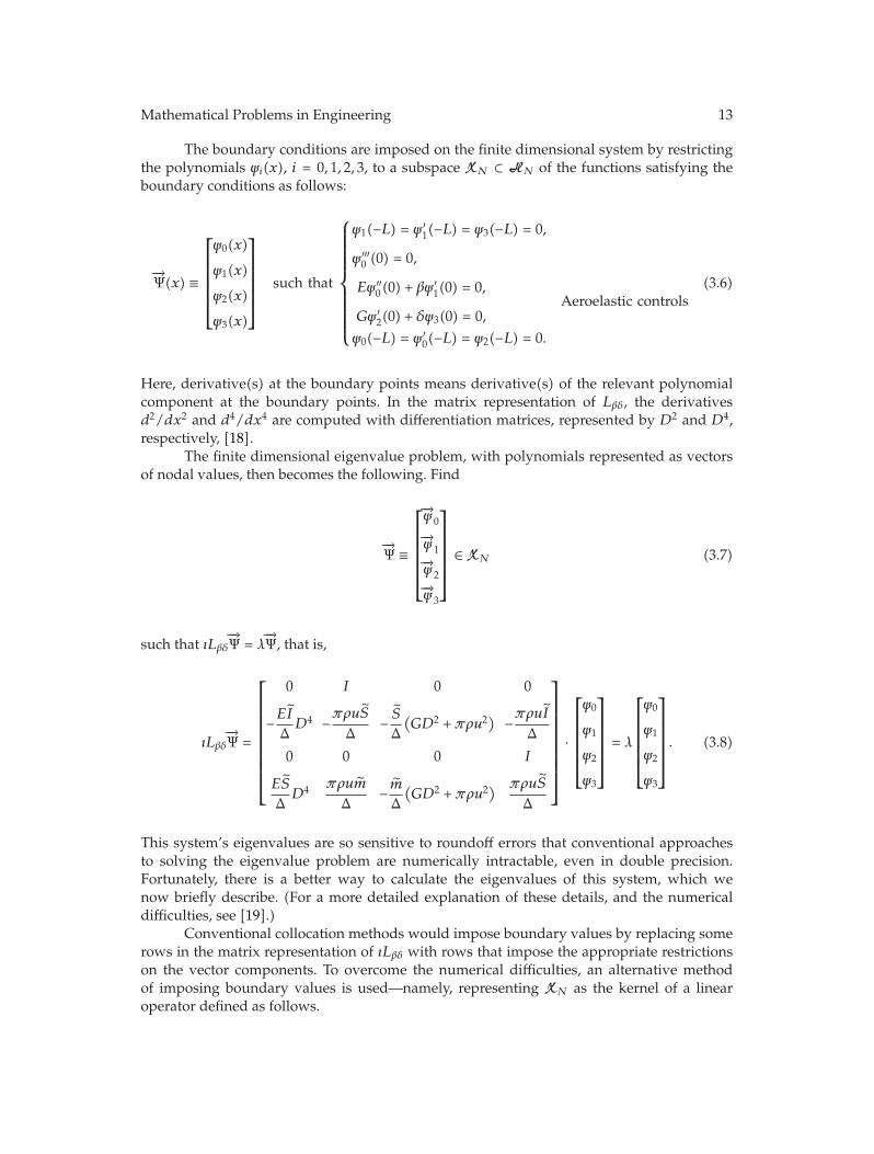
The boundary conditions are imposed on the finite dimensional system by restrictingthe polynomials ψi(x), i = 0, 1, 2, 3, to a subspace XN ⊂ HN of the functions satisfying theboundary conditions as follows:
−→Ψ(x) ≡
⎡⎢⎢⎢⎢⎢⎣
ψ0(x)
ψ1(x)
ψ2(x)
ψ3(x)
⎤⎥⎥⎥⎥⎥⎦ such that
⎧⎪⎪⎪⎪⎪⎪⎪⎪⎪⎨⎪⎪⎪⎪⎪⎪⎪⎪⎪⎩
ψ1(−L) = ψ ′1(−L) = ψ3(−L) = 0,
ψ ′′′0 (0) = 0,
Eψ ′′0(0) + βψ
′1(0) = 0,
Gψ ′2(0) + δψ3(0) = 0,
Aeroelastic controls
ψ0(−L) = ψ ′0(−L) = ψ2(−L) = 0.
(3.6)
Here, derivative(s) at the boundary points means derivative(s) of the relevant polynomialcomponent at the boundary points. In the matrix representation of Lβδ, the derivativesd2/dx2 and d4/dx4 are computed with differentiation matrices, represented by D2 and D4,respectively, [18].
The finite dimensional eigenvalue problem, with polynomials represented as vectorsof nodal values, then becomes the following. Find
−→Ψ ≡
⎡⎢⎢⎢⎢⎢⎣
−→ψ0
−→ψ1−→ψ2−→ψ3
⎤⎥⎥⎥⎥⎥⎦ ∈ XN (3.7)
such that ıLβδ−→Ψ = λ
−→Ψ, that is,
ıLβδ−→Ψ =
⎡⎢⎢⎢⎢⎢⎢⎢⎢⎢⎣
0 I 0 0
−EIΔD4 −
πρuS
Δ− SΔ(GD2 + πρu2) −
πρuI
Δ
0 0 0 I
ES
ΔD4 πρum
Δ−mΔ(GD2 + πρu2) πρuS
Δ
⎤⎥⎥⎥⎥⎥⎥⎥⎥⎥⎦·
⎡⎢⎢⎢⎢⎢⎣
ψ0
ψ1
ψ2
ψ3
⎤⎥⎥⎥⎥⎥⎦ = λ
⎡⎢⎢⎢⎢⎢⎣
ψ0
ψ1
ψ2
ψ3
⎤⎥⎥⎥⎥⎥⎦. (3.8)
This system’s eigenvalues are so sensitive to roundoff errors that conventional approachesto solving the eigenvalue problem are numerically intractable, even in double precision.Fortunately, there is a better way to calculate the eigenvalues of this system, which wenow briefly describe. (For a more detailed explanation of these details, and the numericaldifficulties, see [19].)
Conventional collocation methods would impose boundary values by replacing somerows in the matrix representation of ıLβδ with rows that impose the appropriate restrictionson the vector components. To overcome the numerical difficulties, an alternative methodof imposing boundary values is used—namely, representing XN as the kernel of a linearoperator defined as follows.
14 Mathematical Problems in Engineering
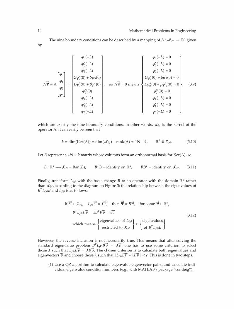
The nine boundary conditions can be described by a mapping of Λ : HN → R9 given
by
Λ−→Ψ ≡ Λ
⎡⎢⎢⎢⎢⎢⎣
ψ0
ψ1
ψ2
ψ3
⎤⎥⎥⎥⎥⎥⎦ =
⎡⎢⎢⎢⎢⎢⎢⎢⎢⎢⎢⎢⎢⎢⎢⎢⎢⎢⎢⎢⎢⎣
ψ0(−L)ψ ′
0(−L)ψ2(−L)
Gψ ′2(0) + δψ3(0)
Eψ ′′0(0) + βψ
′1(0)
ψ ′′′0 (0)
ψ1(−L)ψ ′
1(−L)ψ3(−L)
⎤⎥⎥⎥⎥⎥⎥⎥⎥⎥⎥⎥⎥⎥⎥⎥⎥⎥⎥⎥⎥⎦
, so Λ−→Ψ = 0 means
⎧⎪⎪⎪⎪⎪⎪⎪⎪⎪⎪⎪⎪⎪⎪⎪⎪⎪⎪⎪⎪⎨⎪⎪⎪⎪⎪⎪⎪⎪⎪⎪⎪⎪⎪⎪⎪⎪⎪⎪⎪⎪⎩
ψ0(−L) = 0
ψ ′0(−L) = 0
ψ2(−L) = 0
Gψ ′2(0) + δψ3(0) = 0
Eψ ′′0(0) + βψ
′1(0) = 0
ψ ′′′0 (0) = 0
ψ1(−L) = 0
ψ ′1(−L) = 0
ψ3(−L) = 0
⎫⎪⎪⎪⎪⎪⎪⎪⎪⎪⎪⎪⎪⎪⎪⎪⎪⎪⎪⎪⎪⎬⎪⎪⎪⎪⎪⎪⎪⎪⎪⎪⎪⎪⎪⎪⎪⎪⎪⎪⎪⎪⎭
(3.9)
which are exactly the nine boundary conditions. In other words, XN is the kernel of theoperator Λ. It can easily be seen that
k = dim(Ker(Λ)) = dim(HN) − rank(Λ) = 4N − 9, Rk ∼= XN. (3.10)
Let B represent a 4N × k matrix whose columns form an orthonormal basis for Ker(Λ), so
B : Rk −→ XN = Ran(B), BTB = identity on R
k, BBT = identity on XN. (3.11)
Finally, transform Lβδ with the basis change B to an operator with the domain Rk rather
than XN , according to the diagram on Figure 3: the relationship between the eigenvalues ofBTLβδB and Lβδ is as follows:
If−→Ψ ∈ XN, Lβδ
−→Ψ = λ
−→Ψ, then
−→Ψ = B−→v, for some −→v ∈ R
k,
BTLβδB−→v = λBTB−→v = λ−→v
which means
{eigenvalues of Lβδ
restricted to XN
}⊂{
eigenvalues
of BTLβδB
}.
(3.12)
However, the reverse inclusion is not necessarily true. This means that after solving thestandard eigenvalue problem BTLβδB
−→v = λ−→v , one has to use some criterion to selectthose λ such that LβδB
−→v = λB−→v . The chosen criterion is to calculate both eigenvalues andeigenvectors −→v and choose those λ such that ‖LβδB−→v − λB−→v‖ < ε. This is done in two steps.
(1) Use a QZ algorithm to calculate eigenvalue-eigenvector pairs, and calculate indi-vidual eigenvalue condition numbers (e.g., with MATLAB’s package “condeig”).
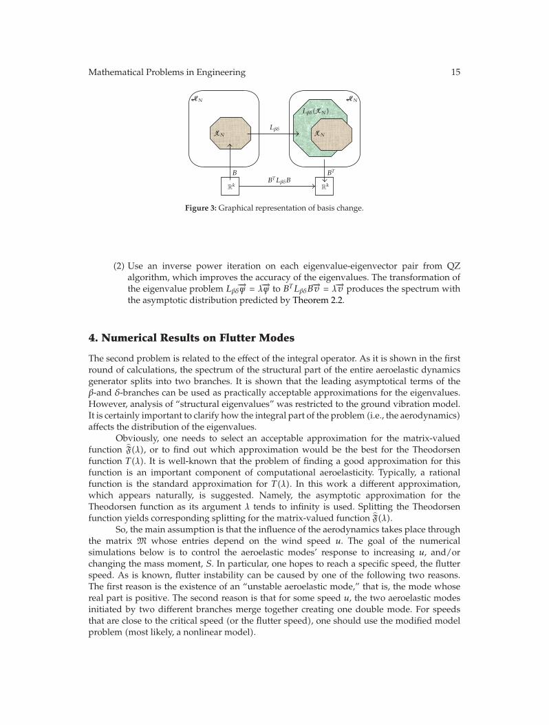
Mathematical Problems in Engineering 15
HN
XN
Lβδ
Rk
BBTLβδB
HN
Lβδ(XN)
XN
BT
Rk
Figure 3: Graphical representation of basis change.
(2) Use an inverse power iteration on each eigenvalue-eigenvector pair from QZalgorithm, which improves the accuracy of the eigenvalues. The transformation ofthe eigenvalue problem Lβδ
−→ψ = λ−→ψ to BTLβδB−→v = λ−→v produces the spectrum with
the asymptotic distribution predicted by Theorem 2.2.
4. Numerical Results on Flutter Modes
The second problem is related to the effect of the integral operator. As it is shown in the firstround of calculations, the spectrum of the structural part of the entire aeroelastic dynamicsgenerator splits into two branches. It is shown that the leading asymptotical terms of theβ-and δ-branches can be used as practically acceptable approximations for the eigenvalues.However, analysis of “structural eigenvalues” was restricted to the ground vibration model.It is certainly important to clarify how the integral part of the problem (i.e., the aerodynamics)affects the distribution of the eigenvalues.
Obviously, one needs to select an acceptable approximation for the matrix-valuedfunction F(λ), or to find out which approximation would be the best for the Theodorsenfunction T(λ). It is well-known that the problem of finding a good approximation for thisfunction is an important component of computational aeroelasticity. Typically, a rationalfunction is the standard approximation for T(λ). In this work a different approximation,which appears naturally, is suggested. Namely, the asymptotic approximation for theTheodorsen function as its argument λ tends to infinity is used. Splitting the Theodorsenfunction yields corresponding splitting for the matrix-valued function F(λ).
So, the main assumption is that the influence of the aerodynamics takes place throughthe matrix M whose entries depend on the wind speed u. The goal of the numericalsimulations below is to control the aeroelastic modes’ response to increasing u, and/orchanging the mass moment, S. In particular, one hopes to reach a specific speed, the flutterspeed. As is known, flutter instability can be caused by one of the following two reasons.The first reason is the existence of an “unstable aeroelastic mode,” that is, the mode whosereal part is positive. The second reason is that for some speed u, the two aeroelastic modesinitiated by two different branches merge together creating one double mode. For speedsthat are close to the critical speed (or the flutter speed), one should use the modified modelproblem (most likely, a nonlinear model).
16 Mathematical Problems in Engineering
Eigenvalues of L − i∗M at tolerance = 1e − 005β = 0 + 1i, δ = 100,N = 80, S = 0.0597, u = 2.1
3000200010000−1000−2000−3000
Real axis
−0.5
0
0.5
1
Imag
inar
yax
is
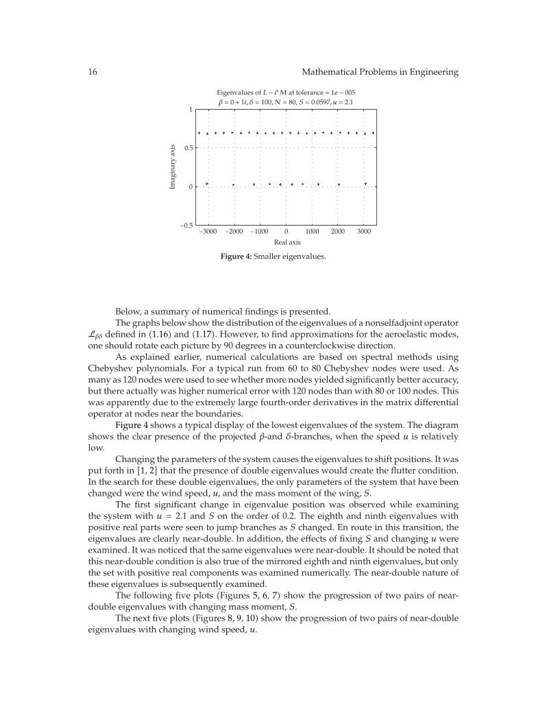
Figure 4: Smaller eigenvalues.
Below, a summary of numerical findings is presented.The graphs below show the distribution of the eigenvalues of a nonselfadjoint operator
Lβδ defined in (1.16) and (1.17). However, to find approximations for the aeroelastic modes,one should rotate each picture by 90 degrees in a counterclockwise direction.
As explained earlier, numerical calculations are based on spectral methods usingChebyshev polynomials. For a typical run from 60 to 80 Chebyshev nodes were used. Asmany as 120 nodes were used to see whether more nodes yielded significantly better accuracy,but there actually was higher numerical error with 120 nodes than with 80 or 100 nodes. Thiswas apparently due to the extremely large fourth-order derivatives in the matrix differentialoperator at nodes near the boundaries.
Figure 4 shows a typical display of the lowest eigenvalues of the system. The diagramshows the clear presence of the projected β-and δ-branches, when the speed u is relativelylow.
Changing the parameters of the system causes the eigenvalues to shift positions. It wasput forth in [1, 2] that the presence of double eigenvalues would create the flutter condition.In the search for these double eigenvalues, the only parameters of the system that have beenchanged were the wind speed, u, and the mass moment of the wing, S.
The first significant change in eigenvalue position was observed while examiningthe system with u = 2.1 and S on the order of 0.2. The eighth and ninth eigenvalues withpositive real parts were seen to jump branches as S changed. En route in this transition, theeigenvalues are clearly near-double. In addition, the effects of fixing S and changing u wereexamined. It was noticed that the same eigenvalues were near-double. It should be noted thatthis near-double condition is also true of the mirrored eighth and ninth eigenvalues, but onlythe set with positive real components was examined numerically. The near-double nature ofthese eigenvalues is subsequently examined.
The following five plots (Figures 5, 6, 7) show the progression of two pairs of near-double eigenvalues with changing mass moment, S.
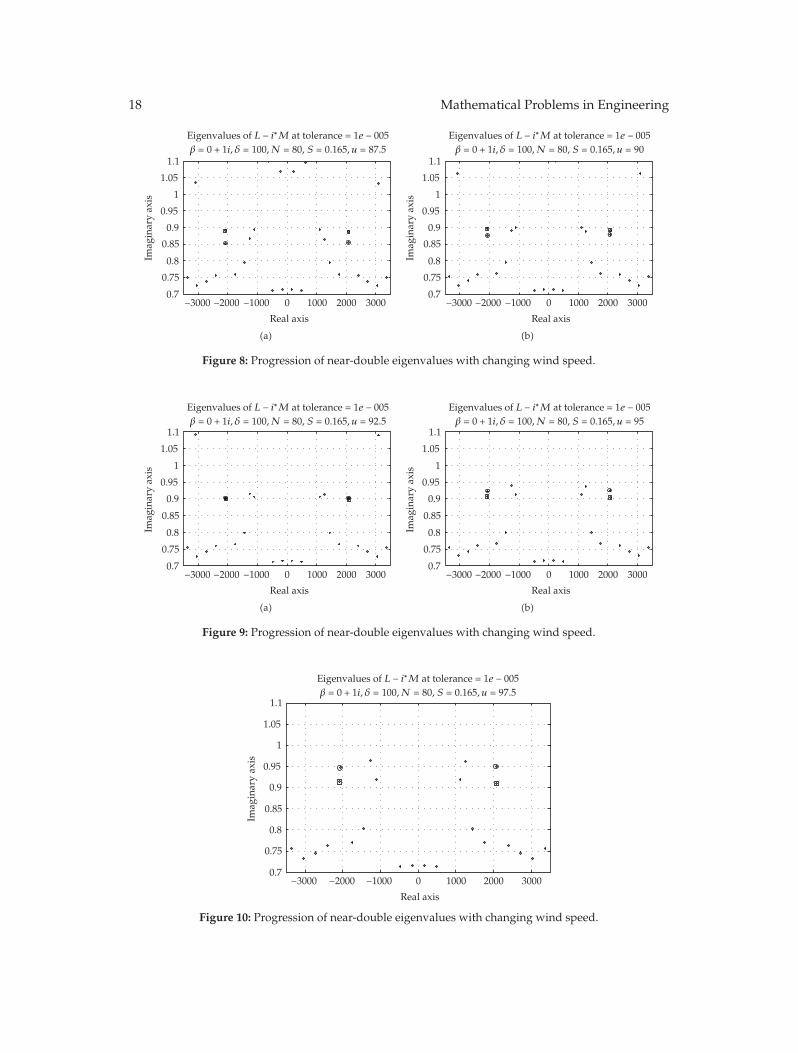
The next five plots (Figures 8, 9, 10) show the progression of two pairs of near-doubleeigenvalues with changing wind speed, u.

Mathematical Problems in Engineering 17
Eigenvalues of L − i∗M at tolerance = 1e − 005β = 0 + 1i, δ = 100,N = 80, S = 0.1597, u = 2.1
3000200010000−1000−2000−3000
Real axis
−0.5
0
0.5
1Im
agin
ary
axis
(a)
Eigenvalues of L − i∗M at tolerance = 1e − 005β = 0 + 1i, δ = 100,N = 80, S = 0.1797, u = 2.1
3000200010000−1000−2000−3000
Real axis
−0.5
0
0.5
1
Imag
inar
yax
is
(b)
Figure 5: Progression of near-double eigenvalues with changing mass moment.
Eigenvalues of L − i∗M at tolerance = 1e − 005β = 0 + 1i, δ = 100,N = 80, S = 0.1997, u = 2.1
3000200010000−1000−2000−3000
Real axis
−0.5
0
0.5
1
Imag
inar
yax
is
(a)
Eigenvalues of L − i∗M at tolerance = 1e − 005β = 0 + 1i, δ = 100,N = 80, S = 0.2197, u = 2.1
3000200010000−1000−2000−3000
Real axis
−0.5
0
0.5
1
Imag
inar
yax
is
(b)
Figure 6: Progression of near-double eigenvalues with changing mass moment.
Eigenvalues of L − i∗M at tolerance = 1e − 005β = 0 + 1i, δ = 100,N = 80, S = 0.2397, u = 2.1
3000200010000−1000−2000−3000
Real axis
−0.5
0
0.5
1
Imag
inar
yax
is
Figure 7: Progression of near-double eigenvalues with changing mass moment.
18 Mathematical Problems in Engineering
Eigenvalues of L − i∗M at tolerance = 1e − 005β = 0 + 1i, δ = 100,N = 80, S = 0.165, u = 87.5
3000200010000−1000−2000−3000
Real axis
0.7
0.75
0.8
0.85
0.9
0.95
1
1.05
1.1Im
agin
ary
axis
(a)
Eigenvalues of L − i∗M at tolerance = 1e − 005β = 0 + 1i, δ = 100,N = 80, S = 0.165, u = 90
3000200010000−1000−2000−3000
Real axis
0.7
0.75
0.8
0.85
0.9
0.95
1
1.05
1.1
Imag
inar
yax
is
(b)
Figure 8: Progression of near-double eigenvalues with changing wind speed.
Eigenvalues of L − i∗M at tolerance = 1e − 005β = 0 + 1i, δ = 100,N = 80, S = 0.165, u = 92.5
3000200010000−1000−2000−3000
Real axis
0.7
0.75
0.8
0.85
0.9
0.95
1
1.05
1.1
Imag
inar
yax
is
(a)
Eigenvalues of L − i∗M at tolerance = 1e − 005β = 0 + 1i, δ = 100,N = 80, S = 0.165, u = 95
3000200010000−1000−2000−3000
Real axis
0.7
0.75
0.8
0.85
0.9
0.95
1
1.05
1.1
Imag
inar
yax
is
(b)
Figure 9: Progression of near-double eigenvalues with changing wind speed.
Eigenvalues of L − i∗M at tolerance = 1e − 005β = 0 + 1i, δ = 100,N = 80, S = 0.165, u = 97.5
3000200010000−1000−2000−3000
Real axis
0.7
0.75
0.8
0.85
0.9
0.95
1
1.05
1.1
Imag
inar
yax
is
Figure 10: Progression of near-double eigenvalues with changing wind speed.
Mathematical Problems in Engineering 19
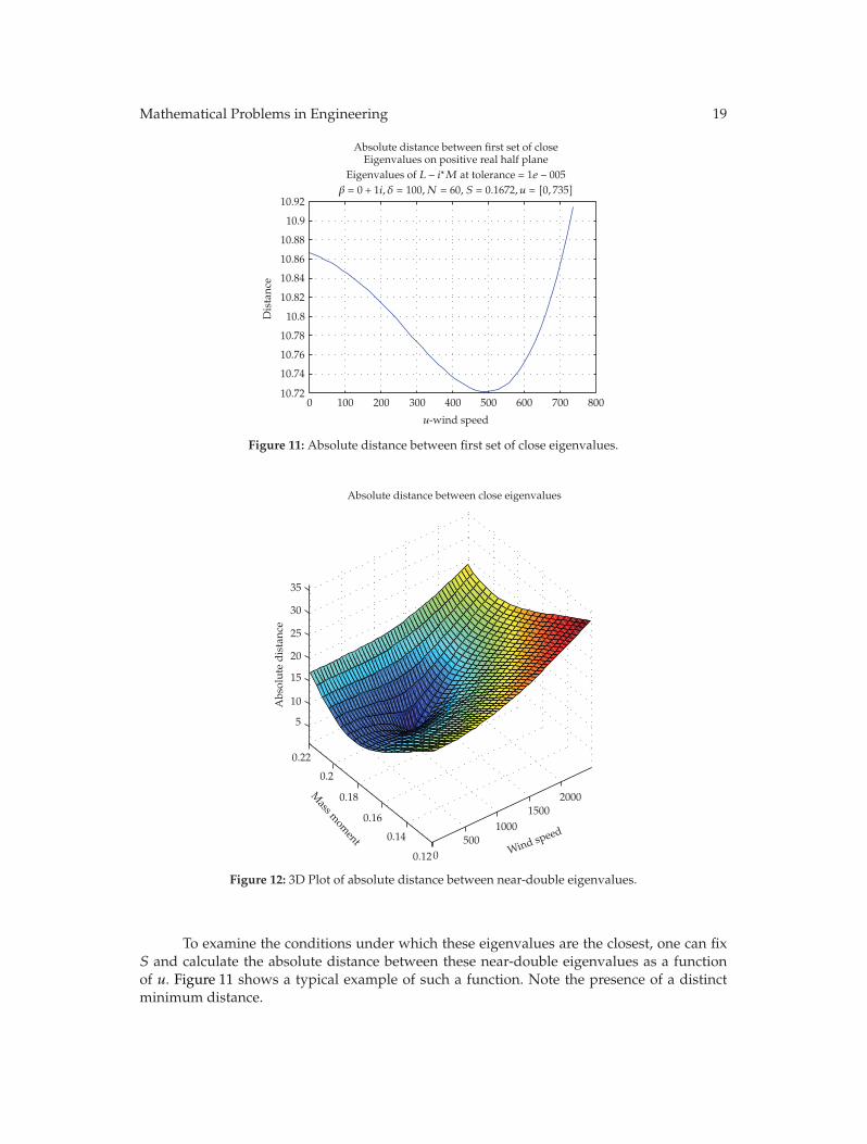
Absolute distance between first set of closeEigenvalues on positive real half plane
Eigenvalues of L − i∗M at tolerance = 1e − 005β = 0 + 1i, δ = 100,N = 60, S = 0.1672, u = [0, 735]
8007006005004003002001000
u-wind speed
10.72
10.74
10.76
10.78
10.8
10.82
10.84
10.86
10.88
10.9
10.92
Dis
tanc
e
Figure 11: Absolute distance between first set of close eigenvalues.
Absolute distance between close eigenvalues
0500
10001500
2000
Wind speed
0.12
0.14
0.16
0.18
0.2
0.22
Mass m
oment
5
10
15
20
25
30
35
Abs
olut
ed
ista
nce
Figure 12: 3D Plot of absolute distance between near-double eigenvalues.
To examine the conditions under which these eigenvalues are the closest, one can fixS and calculate the absolute distance between these near-double eigenvalues as a functionof u. Figure 11 shows a typical example of such a function. Note the presence of a distinctminimum distance.
20 Mathematical Problems in Engineering
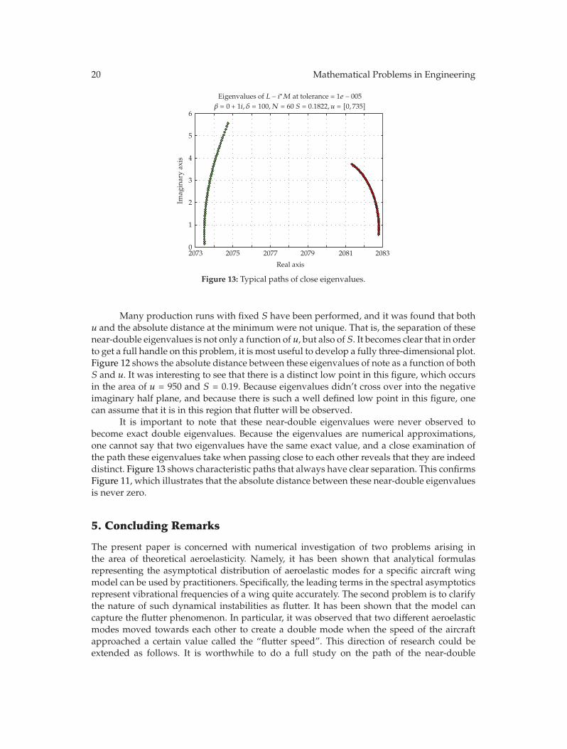
Eigenvalues of L − i∗M at tolerance = 1e − 005β = 0 + 1i, δ = 100,N = 60 S = 0.1822, u = [0, 735]
208320812079207720752073
Real axis
0
1
2
3
4
5
6
Imag
inar
yax
is
Figure 13: Typical paths of close eigenvalues.
Many production runs with fixed S have been performed, and it was found that bothu and the absolute distance at the minimum were not unique. That is, the separation of thesenear-double eigenvalues is not only a function of u, but also of S. It becomes clear that in orderto get a full handle on this problem, it is most useful to develop a fully three-dimensional plot.Figure 12 shows the absolute distance between these eigenvalues of note as a function of bothS and u. It was interesting to see that there is a distinct low point in this figure, which occursin the area of u = 950 and S = 0.19. Because eigenvalues didn’t cross over into the negativeimaginary half plane, and because there is such a well defined low point in this figure, onecan assume that it is in this region that flutter will be observed.
It is important to note that these near-double eigenvalues were never observed tobecome exact double eigenvalues. Because the eigenvalues are numerical approximations,one cannot say that two eigenvalues have the same exact value, and a close examination ofthe path these eigenvalues take when passing close to each other reveals that they are indeeddistinct. Figure 13 shows characteristic paths that always have clear separation. This confirmsFigure 11, which illustrates that the absolute distance between these near-double eigenvaluesis never zero.
5. Concluding Remarks
The present paper is concerned with numerical investigation of two problems arising inthe area of theoretical aeroelasticity. Namely, it has been shown that analytical formulasrepresenting the asymptotical distribution of aeroelastic modes for a specific aircraft wingmodel can be used by practitioners. Specifically, the leading terms in the spectral asymptoticsrepresent vibrational frequencies of a wing quite accurately. The second problem is to clarifythe nature of such dynamical instabilities as flutter. It has been shown that the model cancapture the flutter phenomenon. In particular, it was observed that two different aeroelasticmodes moved towards each other to create a double mode when the speed of the aircraftapproached a certain value called the “flutter speed”. This direction of research could beextended as follows. It is worthwhile to do a full study on the path of the near-double

Mathematical Problems in Engineering 21
eigenvalues. The paths that they take while moving past each other may indicate theconditions in which flutter is most rapidly approached. This information may prove usefulwhen an aircraft changes the angle of attack to circumvent flutter. A more important futureresearch will involve the examination of other near-double eigenvalues of this system. It isshown that this near-double condition is not unique to the eigenvalues examined in thispaper. However, we do not yet know whether these additional eigenvalues can be trustednumerically to be near-double. Also, it is not yet known what their minimum absoluteseparation is, and if it is small enough to produce flutter.
Another future step in this project will be to include the full integral operator. Thiswould be a more complete physical model of the system, and we expect that it will yieldmore accurate results. However, it will no doubt be more demanding computationally.
Acknowledgment
This work was partialy supported by the National Science Foundation Grant DMS-0604842which is highly appreciated by the first author.
References
[1] R. L. Bisplinghoff, H. Ashley, and R. L. Halfman, Aeroelasticity, Dover, New York, NY, USA, 1996.[2] Y. C. Fung, An Introduction to the Theory of Aeroelasticity, Dover, New York, NY, USA, 1993.[3] J. Lutgen, “A note on Riesz bases of eigenvectors of certain holomorphic operator-functions,” Journal
of Mathematical Analysis and Applications, vol. 255, no. 1, pp. 358–373, 2001.[4] M. A. Shubov, “Riesz basis property of root vectors of non-self-adjoint operators generated by aircraft
wing model in subsonic airflow,” Mathematical Methods in the Applied Sciences, vol. 23, no. 18, pp.1585–1615, 2000.
[5] A. V. Balakrishnan and M. A. Shubov, “Asymptotic and spectral properties of operator-valuedfunctions generated by aircraft wing model,” Mathematical Methods in the Applied Sciences, vol. 27,no. 3, pp. 329–362, 2004.
[6] M. A. Shubov, “Asymptotic analysis of aircraft wing model in subsonic air flow,” IMA Journal ofApplied Mathematics, vol. 66, no. 4, pp. 319–356, 2001.
[7] M. A. Shubov, A. V. Balakrishnan, and C. A. Peterson, “Spectral properties of nonselfadjoint operatorsgenerated by coupled Euler-Bernoulli and Timoshenko beam model,” Zeitschrift fur AngewandteMathematik und Mechanik, vol. 84, no. 2, 2004.
[8] M. A. Shubov, “Asymptotic representations for root vectors of nonselfadjoint operators and pencilsgenerated by an aircraft wing model in subsonic air flow,” Journal of Mathematical Analysis andApplications, vol. 260, no. 2, pp. 341–366, 2001.
[9] A. V. Balakrishnan, “Subsonic flutter suppression using self-straining actuators,” Journal of the FranklinInstitute, vol. 338, no. 2-3, pp. 149–170, 2001.
[10] A. V. Balakrishan, “Aeroelastic control with self-straining actuators: continuum models,” in SmartStructures and Materials, Mathematics Control in Smart Structures, V. Vasunradan, Ed., vol. 3323 ofProceedings of SPIE, pp. 44–54, 1998.
[11] A. V. Balakrishnan and J. W. Edwards, “Calculation of the transient motion of elastic airfoils forcedby control surface motion and gusts,” Tech. Rep. NASA TM 81351, 1980.
[12] A. V. Balakrishnan, “Damping performance of strain actuated beams,” Computational and AppliedMathematics, vol. 18, no. 1, pp. 31–86, 1999.
[13] C.-K. Lee, W.-W. Chiang, and T. C. O’Sullivan, “Piezoelectric modal sensor/actuator pairs for criticalactive damping vibration control,” Journal of the Acoustical Society of America, vol. 90, no. 1, pp. 374–384, 1991.
[14] M. A. Shubov and C. A. Peterson, “Asymptotic distribution of eigenfrequencies for coupledEuler–Bernoulli/Timoshenko beam model,” NASA NASA/CR-2003-212022, NASA Dryden Center,November 2003.

22 Mathematical Problems in Engineering
[15] M. A. Shubov, “Asymptotics of aeroelastic modes and basis property of mode shapes for aircraft wingmodel,” Journal of the Franklin Institute, vol. 338, no. 2-3, pp. 171–185, 2001.
[16] I. C. Gohberg and M. G. Krein, Introduction to the Theory of Linear Nonselfadjoint Operators, vol. 18 ofTranslations of Mathematical Monographs, American Mathematical Society, Providence, RI, USA, 1969.
[17] M. Abramowitz and I. Stegun, Eds., Handbook of Mathematical Functions, Dover, New York, NY, USA,1972.

Mathematical Problems in Engineering 23
[18] J. C. Mason and D. C. Handscomb, Chebyshev Polynomials, Chapman & Hall/CRC, Boca Raton, Fla,USA, 2003.
[19] M. A. Shubov and S. Wineberg, “Asymptotic distribution of the aeroelastic modes for wing flutterproblem: numerical analysis,” under review.

Submit your manuscripts athttp://www.hindawi.com
Hindawi Publishing Corporationhttp://www.hindawi.com Volume 2014
MathematicsJournal of
Hindawi Publishing Corporationhttp://www.hindawi.com Volume 2014
Mathematical Problems in Engineering
Hindawi Publishing Corporationhttp://www.hindawi.com
Differential EquationsInternational Journal of
Volume 2014
Applied MathematicsJournal of
Hindawi Publishing Corporationhttp://www.hindawi.com Volume 2014
Probability and StatisticsHindawi Publishing Corporationhttp://www.hindawi.com Volume 2014
Journal of
Hindawi Publishing Corporationhttp://www.hindawi.com Volume 2014
Mathematical PhysicsAdvances in
Complex AnalysisJournal of
Hindawi Publishing Corporationhttp://www.hindawi.com Volume 2014
OptimizationJournal of
Hindawi Publishing Corporationhttp://www.hindawi.com Volume 2014
CombinatoricsHindawi Publishing Corporationhttp://www.hindawi.com Volume 2014
International Journal of
Hindawi Publishing Corporationhttp://www.hindawi.com Volume 2014
Operations ResearchAdvances in
Journal of
Hindawi Publishing Corporationhttp://www.hindawi.com Volume 2014
Function Spaces
Abstract and Applied AnalysisHindawi Publishing Corporationhttp://www.hindawi.com Volume 2014
International Journal of Mathematics and Mathematical Sciences
Hindawi Publishing Corporationhttp://www.hindawi.com Volume 2014
The Scientific World JournalHindawi Publishing Corporation http://www.hindawi.com Volume 2014
Hindawi Publishing Corporationhttp://www.hindawi.com Volume 2014
Algebra
Discrete Dynamics in Nature and Society
Hindawi Publishing Corporationhttp://www.hindawi.com Volume 2014
Hindawi Publishing Corporationhttp://www.hindawi.com Volume 2014
Decision SciencesAdvances in
Discrete MathematicsJournal of
Hindawi Publishing Corporationhttp://www.hindawi.com
Volume 2014 Hindawi Publishing Corporationhttp://www.hindawi.com Volume 2014
Stochastic AnalysisInternational Journal of
Related Documents