Numerical Implementation of Two Nonconforming Finite ...phild/Publications/CMAME1.pdfNumerical Implementation of Two Nonconforming Finite Element Methods for Unilateral Contact Patrick

Comput. Methods Appl. Mech. Engrg., Vol. 184, Issue 1, 99-123 (2000).

Numerical Implementation of Two NonconformingFinite Element Methods for Unilateral Contact

Patrick HILD ∗

Mathematiques pour l’Industrie et la Physique,Unite Mixte de Recherches CNRS–UPS–INSAT (U.M.R. 5640),

Universite Paul Sabatier, 118 route de Narbonne, 31062 TOULOUSE Cedex 4, France.

We consider the finite element approximation of the unilateral contact problem betweenelastic bodies. We are interested in a practical problem which often occurs in finite ele-ment computations concerning two independently discretized bodies in unilateral contact.It follows that the nodes of both bodies located on the contact surface do not fit together.We present two different approaches in order to define unilateral contact on non-matchingmeshes. The first is an extension of the mortar finite element method to variational inequal-ities that defines the contact in a global way. On the contrary, the second one expresses localnode-on-segment contact conditions. In both cases, the theoretical approximation propertiesare given. Then, we implement and compare the two methods.

Keywords : Unilateral Contact, Non-Matching Meshes, Mortar Finite Element Method,Global Contact Condition, Local Contact Condition.

1. INTRODUCTION AND NOTATIONS

In finite element procedures solving unilateral contact problems between deformablebodies, each solid is often discretized independently of the other. So, a finite elementmesh does not coincide with the other one on the contact zone. For instance, consti-tutive or geometrical non-linearities lead to the use of an incremental scheme and, ateach step, the updated finite element meshes cannot fit together on the contact zone.In other respects, mesh adaptivity procedures used in a contact context generally leadto non-matching meshes. So the question is to define a convenient discrete contactcondition for non-matching meshes.

On the one hand, the mathematical framework associated with the finite elementapproximation for contact problems can be found in 16. In this reference, Haslinger,Hlavacek and Necas consider the case of matching meshes on the contact zone.

On the other hand, the mortar element domain decomposition method introducedby Bernardi, Maday and Patera,8 allows the handling of non-matching meshes. Thistechnique has been studied for many problems governed by variational equalities.

∗Actual address : Laboratoire de Mathematiques, Equipe EDP, Universite de Savoie, 73376 LeBourget du Lac Cedex, France.

1

P. Hild / Two nonconforming finite element methods 2

The first extension of the mortar finite element method to a variational inequalityhas been made for the unilateral contact problem by Ben Belgacem, Hild and Labordein 5. In this reference, the authors also extend the finite element analysis of contactproblems to non-matching meshes.

The main aim of this paper is to carry out the first numerical experiments associ-ated with the theoretical results already obtained. The paper is organized as follows.First, we introduce the model describing the unilateral contact without friction be-tween two deformable elastic bodies. The associated weak formulation is exhibited.

Then, in the third section, we consider two finite element methods in order tosolve the problem with independent meshes. The first approach is of global type andcorresponds to an extension of the mortar domain decomposition method. The secondapproximation is of local type and uses classical node-on-segment contact conditions.We recall the most significant approximation properties obtained in previous papersand we establish new results proving the optimal convergence of the global approachand the convergence of the local approach.

In the fourth section, we obtain the corresponding matrix formulations and wemention the algorithm contained in the finite element code CASTEM 2000. The nextsection is devoted to the studies in which the contact conditions are compared froma numerical point of view.

2. SETTING OF THE PROBLEM

We consider two elastic bodies occupying in the initial configuration two subsets Ωℓ

of R2, ℓ = 1, 2. The boundary ∂Ωℓ of the domain Ωℓ is assumed to be “smooth” and

consists of three nonoverlapping parts Γℓu, Γℓ

g and Γℓc. The unit outward normal on ∂Ωℓ

is denoted nℓ. The body is submitted to volume forces f ℓ on Ωℓ and to surface forcesgℓ on Γℓ

g. On Γℓu, the displacements Uℓ are prescribed. In the initial configuration,

both bodies have a common portion Γc = Γ1c = Γ2

c which will be considered as thecandidate contact surface for the sake of simplicity.

The unilateral contact problem consists of finding the displacement field u =(u1,u2) where uℓ = u|Ωℓ and the stress tensor field σ = (σ1, σ2), (σℓ = σ|Ωℓ) satisfyingthe following conditions (2.1)–(2.5) for ℓ = 1, 2 :

div σℓ(uℓ) + f ℓ = 0 in Ωℓ,

σℓ(uℓ)nℓ = gℓ on Γℓg, (2.1)

uℓ =Uℓ on Γℓu.

The symbol div denotes the divergence operator defined by div σ =(

∂σij

∂xj

)

iwhere

the summation convention of repeated indices is adopted.We will consider small strains hypothesis so that the strain tensor ε(v) induced by

a displacement field v is ε(v) = (∇v + t∇v)/2. The stress tensor field σℓ is linked tothe displacement field uℓ by the constitutive law of linear elasticity

σℓ(uℓ) = Cℓ ε(uℓ), (2.2)


where Cℓ = (cℓij,kh)1≤i,j,k,h≤2 is a fourth order tensor satisfying cℓij,kh = cℓji,kh = cℓkh,ij.We assume that there exists constants αℓ > 0 verifying

cℓij,kh εij εkh ≥ αℓ εij εij, ∀εij = εji.

The conditions on the contact zone Γc are as follows

(σ1(u1)n1).n1 = (σ2(u2)n2).n2 =σn(u), (2.3)

u1.n1 + u2.n2 ≤ 0, σn(u) ≤ 0, σn(u)(u1.n1 + u2.n2) = 0, (2.4)

σ1T(u1) = σ2

T(u2) = 0, (2.5)

whereσℓ

T(uℓ) = σℓ(uℓ)nℓ − σn(u)nℓ, 1 ≤ ℓ ≤ 2.

The relations (2.3) represent the action and the reaction principle. The conditions(2.4) express unilateral contact between the two bodies and finally (2.5) states acontact without friction.

In order to obtain the variational formulation of the problem, we introduce thespaces V(Ωℓ), (ℓ = 1, 2)

V(Ωℓ) =

v ∈(

H1(Ωℓ))2, v = Uℓ on Γℓ

u

,

where H1(Ωℓ) is the classical Sobolev space (see 1). A vector field v ∈ V(Ω1)×V(Ω2)is denoted v = (v1,v2). Endowed with the standard inner product

(u,v) = (u1,v1)(H1(Ω1))2 + (u2,v2)(H1(Ω2))2 ,

V(Ω1)×V(Ω2) is a Hilbert space and the corresponding energy norm is denoted ‖.‖.We define the bilinear form

a(u,v) =2

∑

ℓ=1

∫

ΩℓCℓ ε(uℓ).ε(vℓ) dΩℓ,

for all u,v ∈ V(Ω1)×V(Ω2). Next, we denote L(.) the linear form which correspondsto the external loads:

L(v) =2

∑

ℓ=1

(

∫

Ωℓf ℓ.vℓ dΩℓ +

∫

Γℓg

gℓ.vℓ dΓℓ)

.

The closed convex set K of admissible displacements is the subset of V(Ω1)×V(Ω2)which contains the displacement fields satisfying the non-penetration condition:

K =

v = (v1,v2) ∈ V(Ω1) × V(Ω2), v1.n1 + v2.n2 ≤ 0 on Γc

.

The variational inequality associated with the unilateral contact problem (2.1)-(2.5) consists of finding u such that (see 13,16,21):

u ∈ K, a(u,v − u) ≥ L(v − u), ∀v ∈ K. (2.6)


Using Stampacchia’s theorem, we conclude that problem (2.6) has only one solutionwhen (for example) Γℓ

u, ℓ = 1, 2 is of positive measure. Other conditions leading toexistence and uniqueness results can be found in 16.Remark 2.1. The more general and technical study involving an initial gap and thecorresponding results are given in 16, chapter 3, sections 5-6.

3. THE FINITE ELEMENT APPROXIMATION FOR NON-MATCHING

MESHES

3.1. The global and the local contact conditions

We suppose that Ω1 and Ω2 are domains with polygonal boundaries and weassume that Γc is a straight line segment to simplify. Let the approximation parameterh = (h1, h2) be a given pair of real positive numbers that will decay to 0. With eachsubdomain Ωℓ, we then associate a family of triangulations T ℓ

h, made of trianglesdenoted κ, the diameter of which does not exceed hℓ. Therefore, we can write

Ωℓ=

⋃

κ∈T ℓh

κ.

The extreme points c1 and c2 of the contact part Γc are supposed to belong to bothmeshes associated with T 1

h and T 2h . The contact zone Γc inherits two independent

families of discretizations arising from T 1h and T 2

h . The mesh T ℓc,h on Γc is defined as

the set of all the edges of κ ∈ T ℓh on the contact zone. The set of the nodes associated

with T ℓc,h is denoted ξℓ

h. In general ξ1h and ξ2

h are not identical on account of thenon-matching meshes.

The space of the polynomials on κ whose global degree is lower or equal toq, (q nonnegative integer) is denoted Pq(κ). The finite element space used in Ωℓ

is then defined as (see 11):

Vh(Ωℓ) =

vℓh ∈ (C(Ω

ℓ))2, ∀κ ∈ T ℓ

h, vℓh|κ ∈ (P1(κ))

2, vℓh|Γℓ

u= Uℓ

h

,

where C(Ωℓ) denotes the space of continuous functions on Ω

ℓand Uℓ

h is a finite elementapproximation of Uℓ.

In order to express the contact constraints (2.4) on Γc, we need to introduce somefunctional spaces. Let W ℓ

h(Γc) be the range of Vh(Ωℓ) by the normal trace operator

on Γc:W ℓ

h(Γc) =

ϕh = vℓh|Γc

.nℓ, vℓh ∈ Vh(Ω

ℓ)

. (3.1)

Next, we introduce the space of the Lagrange multipliers that will be useful to definea projection operator:

M ℓh(Γc) =

ψh ∈W ℓh(Γc), ψh|T ∈ P0(T ), ∀T ∈ T ℓ

c,h, such that c1 or c2 ∈ T

.

The notation πℓh stands for the projection operator on W ℓ

h(Γc) defined for any functionϕ ∈ C(Γc) as

πℓhϕ ∈W ℓ

h(Γc),


(πℓhϕ)(ci) =ϕ(ci), for i = 1 and 2, (3.2)

∫

Γc

(ϕ− πℓhϕ)ψh dΓ = 0, ∀ψh ∈M ℓ

h(Γc).

The condition (πℓhϕ)(ci) = ϕ(ci), i = 1, 2, has been introduced in order to handle

more general problems in a domain decomposition context (see 8). It is easy to checkthat the classical L2 projection operator on W ℓ

h(Γc) does not satisfy such a condition.The approximation properties of πℓ

h are enumerated in Ben Belgacem, 4.By using this projection operator (of global character), we are in a position to

define the discrete admissibility convex cone Kgloh :

Kgloh =

vh = (v1h,v

2h) ∈ Vh(Ω

1) × Vh(Ω2), v1

h.n1 + π1

h(v2h.n

2) ≤ 0 on Γc

. (3.3)

Let us notice that the condition incorporated in Kgloh is expressed in the space W 1

h (Γc).Following the terminology of Bernardi, Maday and Patera 8, W 2

h (Γc) stands for themortar space.Remark 3.1. Of course, it is possible to give a symmetrical definition of the convexby choosing as mortar space W 1

h (Γc) and using the projection operator π2h.

Let Iℓh denote the Lagrange interpolation operator ranging in W ℓ

h(Γc). Then, wedefine the admissibility convex cone Kloc

h by using the interpolation operator of localcharacter:

Kloch =

vh = (v1h,v

2h) ∈ Vh(Ω

1) × Vh(Ω2), v1

h.n1 + I1

h(v2h.n

2) ≤ 0 on Γc

. (3.4)

The discrete local contact conditions inserted in the definition of Kloch are similar to

the classical node-on-segment conditions.Remark 3.2. There are other possibilities of defining unilateral contact with non-matching meshes (see 7,12,17).

In addition, it is straightforward to check that Kgloh 6⊂ K and Kloc

h 6⊂ K. Therefore,both approximations are not “Hodge” conforming (see 11). When matching meshesare used, the discrete unilateral constraints can be expressed in both cases merelyby the natural node-on-node condition v1

h.n1 + v2

h.n2 ≤ 0 and the approximation

becomes conforming (Kgloh = Kloc

h ⊂ K). This situation was extensively studied byHaslinger and Hlavacek,15 Haslinger, Hlavacek and Necas,16.

The finite element problem issued from (2.6) is the following variational inequality:find uh such that

uh ∈ Kh, a(uh,vh − uh) ≥ L(vh − uh), ∀vh ∈ Kh, (3.5)

where Kh = Kgloh or Kh = Kloc

h .Using again Stampacchia’s theorem, we conclude that problem (3.5) admits a

unique solution under the assumptions mentioned in the previous section.Remark 3.3. The finite element approximation in the general case of an initial gapbetween the bodies (with matching meshes) and the associated error estimations canbe found in 16, chapter 3, section 8.


3.2. Error estimation

We intend in the present part to give an estimate of the error committed on theexact solution by the global and the local finite element approximations.

In the next theorems, we adopt regularity assumptions which have been intro-duced by Brezzi, Hager and Raviart,9 for a Signorini problem, and used by Haslinger,Hlavacek and Necas,16 for the unilateral contact problem with matching meshes onthe contact zone.

For technical reasons, we assume that the family of triangulations T ℓh is regular (see

11) and that h1/h2 is bounded. Moreover, we suppose that the measure of Γℓu does

not vanish and that Uℓ = 0, ℓ = 1, 2. We will make use of the standard Lebesgue andSobolev spaces L∞,W 1,∞, (Hτ )τ∈R+

; the detailed presentation of these spaces can befound in 1.

The approximation result associated with the global contact case is given in thefollowing theorem.

Theorem 3.1 Suppose that the solution u of the continuous problem (2.6) is suchthat u1 ∈ (H2(Ω1))2, u2 ∈ (H2(Ω2))2, u1.n1 ∈ W 1,∞(Γc), u2.n2 ∈ W 1,∞(Γc) andσn(u) ∈ L∞(Γc). Suppose that the set of points of Γc in which the change fromu1.n1 + u2.n2 < 0 to u1.n1 + u2.n2 = 0 occurs is finite. Let uh be the solution of theproblem (3.5) with Kh = K

gloh . Then

‖u − uh‖ ≤ C(u)(h1 + h2),

where C(u) is independent of h.

Proof. The starting point of the proof consists of a result in 6 which is thefollowing:

‖u − uh‖2 ≤ C2(u)(h21 + h2

2) + C∫

Γc

σn(u)(I1h[u.n] − [u.n]) dΓ

+C(u) h1(‖u − uh‖ + C(u)h2),

where [u.n] = u1.n1 + u2.n2.Then, by writing 2h1h2 ≤ h2

1 + h22 and

2C(u)h1‖u − uh‖ ≤ β‖u − uh‖2 +1

βC2(u)h2

1

for any positive β, it comes out that

‖u − uh‖2 ≤ C2(u)(h21 + h2

2) + C∫

Γc

σn(u)(I1h[u.n] − [u.n]) dΓ, (3.6)

if β is chosen small enough.Using the condition σn(u)(u1.n1 +u2.n2) = 0 on Γc, and writing the integral term

as a sum of integrals on the segments t1h defined by the mesh of Ω1, we obtain∫

Γc

σn(u)(I1h[u.n] − [u.n]) dΓ =

∫

Γc

σn(u)(I1h[u.n]) dΓ,

=∑

t1h∈T 1

c,h

∫

t1h

σn(u)(I1h[u.n]) dΓ.


It is obvious that the integrals which do not involve points of Γc in which the changefrom u1.n1 + u2.n2 < 0 to u1.n1 + u2.n2 = 0 occurs are equal to zero. Therefore, itremains a finite number (independent de h) of integral terms which are bounded byusing the regularity assumptions on the exact solution. This yields

∫

Γc

σn(u)(I1h[u.n] − [u.n]) dΓ =

∑

finite

∫

t1h

σn(u)(I1h[u.n]) dΓ,

≤Ch1‖σn(u)‖L∞(t1h)‖I1

h[u.n]‖L∞(t1h),

≤Ch21‖σn(u)‖L∞(Γc)(‖u1.n1‖W 1,∞(Γc) + ‖u2.n2‖W 1,∞(Γc)).

That concludes the proof.This theorem extends the result by Haslinger, Hlavacek and Necas established for

matching meshes (see 16, Theorem 8.1).Remark 3.4. The smoothness conditions uℓ.nℓ ∈ W 1,∞(Γc), ℓ = 1, 2, σn(u) ∈L∞(Γc) as well as the condition on the finite number of points can be avoided. Indeed,under H2×H2 assumptions on the displacements, the convergence rate of the method

is of the order h3

4

1 + h2 (see 5) as in the matching case (see 16). The latter regularityassumptions can be again weakened, and under Hν ×Hν (3/2 < ν ≤ 2) assumptions,

we obtain a convergence rate of order hν2− 1

4

1 + hν−12 (see 6).

Remark 3.5. It can be proved with a counterexample that the integral term of (3.6)

cannot be bounded below h3

2

1 under H2 ×H2 regularity assumptions (see 19).In the local contact case, we can only obtain the following convergence rate, which

is suboptimal in the finite element sense.Theorem 3.2 Let the assumptions of the previous theorem on u be fulfilled. Let uh

be the solution of problem (3.5) with Kh = Kloch . Then

‖u − uh‖ ≤ C(u)(√

h1 + h2),

where C(u) is independent of h.Proof. By using an analogous estimate with that established in 6, we write

‖u − uh‖2 ≤ C2(u)(h21 + h2

2) + C∫

Γc

σn(u)(I1h[u.n] − [u.n]) dΓ

+C(u)√

h1(‖u − uh‖ + C(u)h2).

Using the same arguments as in the previous theorem yields the result.Remark 3.6. The convergence rate of order

√h1 + h2 comes from the poor ap-

proximation properties of the Lagrange interpolation operator in dual Sobolev spaces(see the counterexample in 19) and therefore it has been proved that the estimates ob-tained in the analysis are optimal. Of course, one could dream that the analysis isinappropriate. The latter question seems to be open.


4. MATRIX FORMULATIONS

When solving the discretized unilateral contact problem, we use the finite el-ement code CASTEM 2000 and a saddle-point formulation in which the multipliersare continuous functions on the contact zone and piecewise linear on the mesh ofΩ1. A minimization type formulation for frictional contact problems can be founde.g. in 23; for an augmented lagrangian approach with non-matching grids in linearelasticity, see 22. A saddle-point formulation in which the multipliers are piecewiseconstant functions on the contact zone can be found in 16,25.

4.1. Preliminaries

At first, we intend to define the closed convex cone Mh of the discrete Lagrangemultipliers. We set

Mh =

λh ∈W 1h (Γc),

∫

Γc

λhϕh dΓ ≤ 0, ∀ϕh ∈W 1h (Γc), ϕh ≥ 0

, (4.1)

where W 1h (Γc) is a space of continuous and piecewise linear functions defined in (3.1).

Remark 4.1. A function belonging to Mh is not necessarily nonpositive on Γc.The following lemma is the tool used in order to bear out the choice of the Lagrange

multipliers convex cone Mh.Lemma 4.1 Let ϕh ∈ W 1

h (Γc). Then

ϕh ≤ 0 if and only if∫

Γc

ϕhψh dΓ ≥ 0, ∀ψh ∈ Mh. (4.2)

Proof. Let us notice that the bilinear form A defined on W 1h (Γc) by

A(θh, ρh) =∫

Γc

θhρh dΓ,

is an inner product on W 1h (Γc). Set

Nh =

ϕh ∈W 1h (Γc), ϕh ≤ 0

,

which is a closed convex cone. Then, we consider the polar cone of Nh, denoted N oh ,

and defined as follows (see 20):

N oh =

ψh ∈ W 1h (Γc),

∫

Γc

ψhϕh dΓ ≤ 0, ∀ϕh ∈ Nh

.

The definition of Mh in (4.1) yields N oh = −Mh. Using the property that the

bipolar cone of a closed convex cone is the same convex cone, we deduce:

Nh = (N oh )o =

ϕh ∈W 1h (Γc),

∫

Γc

ϕhψh dΓ ≤ 0, ∀ϕh ∈ N oh

,

=

ϕh ∈W 1h (Γc),

∫

Γc

ϕhψh dΓ ≥ 0, ∀ϕh ∈ Mh

.

Hence the lemma.


4.2. The global contact case (Kh = Kgloh )

Setting Vh = Vh(Ω1)×Vh(Ω

2), we consider the saddle-point problem on Vh×Mh

associated with the following Lagrangian Lglo:

Lglo(vh, µh) =1

2a(vh,vh) − L(vh) −

∫

Γc

µh(v1h.n

1 + π1h(v

2h.n

2))dΓ. (4.3)

It is easy to verify that there exists a unique saddle-point (uh, λh) on Vh × Mh

and, using (4.2), it comes out that uh is the unique solution of the variational problem(3.5) with Kh = K

gloh . Moreover, it can be also proved that the multiplier λh tends

towards σn(u) if h = (h1, h2) decays to zero; this convergence result is beyond thescope of this paper and it will be established in a forthcoming study.

Denoting by V and U the vectors corresponding to the nodal values of vh and uh

respectively, and by M and Λ the vectors corresponding to the nodal values of µh andλh respectively, the saddle-point problem (4.3) consists of finding (U,Λ) solution to

maxA1M≤0

(

minV

1

2tVKV − tVF − t(BV)A1M

)

, (4.4)

where K is the stiffness matrix, F is a generalized load vector and A1 is the massmatrix associated with the mesh of Ω1 on Γc. This means that A1 is a m-by-m matrixwhere m is the number of nodes of the mesh of Ω1 on Γc, and satisfying

(A1)i,j =∫

Γc

ψiψj dΓ, 1 ≤ i, j ≤ m, (4.5)

where ψi ∈ W 1h (Γc) is equal to one on node number i and to zero on the other nodes.

The matrix B expresses the contact condition and requires the calculation of theprojection operator π1

h mapping W 2h (Γc) into W 1

h (Γc) (see (3.2)). In order to deter-mine B, we need to give the matrix formulation of the condition v1

h.n1 + π1

h(v2h.n

2)incorporated in (3.3) and (4.3). Denoting by n the number of nodes of Ω2 on Γc andby Im the m-by-m identity matrix, we have to find the m-by-(m+ n) matrix:

( Im | Π1h ) , (4.6)

where Π1h is the m-by-n projection operator matrix. We denote by ϕj ∈W 2

h (Γc), 1 ≤j ≤ n, the function equal to one on node number j and to zero on the other nodes.Then, we define θk ∈W 1

h (Γc), 2 ≤ j ≤ m− 1, as follows

θ2 =ψ1 + ψ2,

θk =ψk, 3 ≤ k ≤ m− 2,

θm−1 =ψm−1 + ψm.

Using (3.2), we deduce Π1h = C−1D where C is the following m-by-m matrix:

C1,1 = 1,

C1,j = 0, 2 ≤ j ≤ m,

Ci,j =∫

Γc

θiψj dΓ, 2 ≤ i ≤ m− 1, 1 ≤ j ≤ m,

Cm,j = 0, 1 ≤ j ≤ m− 1,

Cm,m = 1,


and D is the m-by-n matrix verifying

D1,1 = 1,

D1,j = 0, 2 ≤ j ≤ n,

Di,j =∫

Γc

θiϕj dΓ, 2 ≤ i ≤ m− 1, 1 ≤ j ≤ n,

Dm,j = 0, 1 ≤ j ≤ n− 1,

Dm,n = 1.

In order to compute Di,j, 2 ≤ i ≤ m− 1, 1 ≤ j ≤ n, we denote by ξh the set of thenodes located on Γc such that ξh = (ξ1

h ∪ ξ2h) \ (ξ1

h ∩ ξ2h). Denoting by p the number

of nodes in ξh (one has max(m,n) ≤ p ≤ m + n − 2), we introduce the functions(χk)1≤k≤p. The function χk is continuous on Γc, piecewise linear on the mesh definedby ξh, equal to one on node number k and to zero on the other nodes of ξh. As aresult, we write

Di,j =∫

Γc

θiϕj dΓ =∫

Γc

(

p∑

k=1

(αi)kχk

)(

p∑

k=1

(βj)kχk

)

dΓ

=p

∑

k=1

p∑

k′=1

(αi)k(βj)k′

∫

Γc

χkχk′ dΓ.

The determination of the (αi)k and the (βj)k′ is done by taking the values of θi andϕj at the nodes of ξh. The m-by-n projection matrix C−1D is then computed oncefor all. In the current bidimensional context, with the examples we consider (see thenumerical studies), the computation of C−1D is not expensive. Nevertheless, if wewant to adapt and extend to the threedimensional case this global contact procedure,it will certainly be necessary to avoid the complete construction of C−1D.

The solution (U,Λ) of (4.4) satisfies the relation KU − tBA1Λ = F . So, settingΦ = A1M , the saddle-point problem (4.4) can be rewritten as a minimization problemof a quadratic functional with linear inequality constraints:

minΦ≤0

(1

2tΦBK−1tBΦ + tΦBK−1F +

1

2tFK−1F

)

. (4.7)

Since m is the rank of B and K is symmetric and positive definite, it comes outthat the matrix BK−1tB is symmetric and positive definite. If Φ0 is the solutionof the minimization problem (4.7), then Λ = (A1)−1Φ0 and the calculation of U =K−1(F + tBΦ0) is straightforward.

As already noticed in Remark 4.1, the components of the vector Λ (representingσn(u)) are not necessarily nonpositive. In a a posteriori error estimation (see 12), this“lack of non-positiveness” must be added to the error.

The finite element code CASTEM 2000 solves the minimization problem (4.7) byusing the iterative Frank and Wolfe algorithm (see 14) which we recall hereafter.

Consider the problem of minimizing the functional J : Rn → R under linear con-

straints

minΦ≤0

J(Φ). (4.8)


The method of Frank and Wolfe is iterative and generates a sequence of pointsΦ0,Φ1, ...,Φk where ∀k, Φk+1 is defined by using Φk as follows : solve the linearprogramming problem

(LP (Φk)) minΦ≤0

t(∇J(Φk)).Φ (4.9)

Let yk be an extremal point of X = Φ ∈ Rn, C ≤ Φ ≤ 0 (where |C| is chosen large

enough such that X contains a solution of (4.8)) and optimal solution to (LP (Φk)).Then Φk+1 is given by

J(Φk+1) = minΦ∈[Φk,yk]

J(Φ).

If J is continuously differentiable and if J(Φ) → ∞ as ‖Φ‖Rn → ∞, then for everyΦ0 ∈ X, the method converges towards a local minimum of J(Φ), Φ ∈ X, (see 24).Notice that for convex problems, the linear subproblem (4.9) provides a lower boundon the optimal objective value. The upper bound on the objective value is updatedat each step and the algorithm is terminated when the relative difference between thebounds is smaller then a a priori set parameter. The theoretical convergence rate ofthe algorithm is arithmetic (see 26,10).

4.3. The local contact case (Kh = Kloch )

In this case, we consider the saddle-point problem on Vh × Mh associated withthe Lagrangian Lloc:

Lloc(vh, µh) =1

2a(vh,vh) − L(vh) −

∫

Γc

µh(v1h.n

1 + I1h(v2

h.n2))dΓ. (4.10)

As in the global contact case, there exists a unique saddle-point (uh, λh) on Vh ×Mh and, using (4.2), we conclude that uh is the unique solution of (3.5) with Kh =Kloc

h . The study of the convergence of λh towards σn(u) will be proposed in a followingstudy.

The problem (4.10) consists then of solving the minimization problem

minΦ≤0

(1

2tΦB′K−1tB′Φ + tΦB′K−1F +

1

2tFK−1F

)

, (4.11)

where the matrix B′ involves now the local contact conditions. In fact, we need only todetermine the matrix formulation of the Lagrange interpolation operator I1

h mappingW 2

h (Γc) into W 1h (Γc). This is done with the following m-by-n matrix denoted I1

h:

(I1h)i,j = (I1

hϕj)(ai), 1 ≤ i ≤ m, 1 ≤ j ≤ n, (4.12)

where ϕj ∈ W 2h (Γc) is equal to one on the node number j and to zero on the others,

and ai denotes node number i on the mesh of Ω1 on Γc.Problem (4.11) is solved in the finite element code like problem (4.7).

Remark 4.2. In the case where the bodies are supposed to come into contact afterdeformation, we must take into account of the initial gap. So, we replace in (4.7) and


(4.11), BV and B′V by BV−G and B′V−G respectively, where G is the m-vectorwhose components are the distances between the nodes of Ω1 on the candidate contactzone and the boundary of Ω2.Remark 4.3. In order to show concretely the differences between the global contactconditions ant the local node-on-segment conditions, we propose to illustrate theircharacteristics with the simple example depicted in Figure 1.

Ω2

Ω1

Figure 1: A simple example of nonmatching meshes

There are 7 equidistant nodes of Ω1 and 5 equidistant nodes of Ω2 on the contactzone. It is easy to see that the interpolation matrix I1

h defined in (4.12) is given by

I1h =

1.0000 0.0000 0.0000 0.0000 0.00000.3333 0.6666 0.0000 0.0000 0.00000.0000 0.6666 0.3333 0.0000 0.00000.0000 0.0000 1.0000 0.0000 0.00000.0000 0.0000 0.3333 0.6666 0.00000.0000 0.0000 0.0000 0.6666 0.33330.0000 0.0000 0.0000 0.0000 1.0000

whereas the projection matrix Π1h introduced in (4.6) is as follows

Π1h =

1.0000 0.0000 0.0000 0.0000 0.00000.2947 0.7440 −0.0379 −0.0016 0.0008

−0.0566 0.7799 0.2727 0.0080 −0.00400.0152 −0.0303 1.0303 −0.0303 0.0152

−0.0040 0.0080 0.2727 0.7799 −0.05660.0008 −0.0016 −0.0379 0.7740 0.29470.0000 0.0000 0.0000 0.0000 1.0000

Of course, the terms of the matrices I1h and Π1

h are rounded numbers. The localcharacter of the interpolation operator is given by the numerous terms (outside ofthe ‘diagonal’) of the matrix I1

h which are equal to zero. That merely means thatthe nodes which are distant do not interact in the definition of the node-on-segmentconditions. On the contrary, the global character of the projection operator is shownby the non-zero terms of the matrix Π1

h. The terms which are near to 1 representstrong interaction between close nodes of both bodies whereas the terms near to zerocorrespond to little interaction between distant nodes.


5. NUMERICAL STUDIES

In this section, we report numerical studies on several problems dealing withglobal and local contact conditions. The numerical experiments have been made atthe Laboratoire de Mathematiques pour l’Industrie et la Physique of the Universitede Toulouse, at the Laboratoire de Mecanique et Technologie of the Ecole NormaleSuperieure de Cachan and more recently at the Laboratoire de Mathematiques of theUniversite de Savoie. In all three cases, we used the finite element code CASTEM2000.

In accordance with the previous notations of sections 3 and 4, we adopt thisconvention: the upper body always stands for Ω1.

5.1. Test 1: comparison of convergence rates for global, local and node-

on-node conditions

In a previous section, we have considered the theoretical convergence rates ofthe discretized solutions towards the solution u of the continuous problem (2.6). Thistest consists of comparing these convergence rates in a numerical context.

Contact problems generally do not admit an analytical solution. Therefore, wemust have a solution with finely discretized bodies at our disposal, which is a refer-ence solution (denoted uhref

) for error estimates. In order to obtain the convergencecurve of the error, we build a family of nested meshes. This family is obtained byan algorithm which divides the triangles: we begin with a very coarse mesh and thefollowing mesh is obtained by the natural subdivision of each triangle in four trian-gles. We then compute the finite element solution uh on each mesh. As previouslynoticed, the error ‖u − uh‖ is approximated by ‖uhref

− uh‖. The latter expressionis estimated by ‖σh((Ihuhref

) − uh)‖∗ where Ih denotes the Lagrange interpolationoperator, σh((Ihuhref

) − uh) is the stress tensor field associated with (Ihuhref) − uh

and ‖.‖∗ stands for the standard L2(Ω1 ∪ Ω2)-norm defined on the space of tensorfields. The most refined mesh is the reference mesh. For obvious reasons, the errorcan not be estimated by taking uh = uhref

and we choose the most refined mesh forerror computations such that h = 4href . We are interested in the rate of convergence

denoted α such that :‖uhref

− uh‖‖uhref

‖ = Chα1 , where the notation h1 represents the

discretization parameter of the upper body.

• Comparison between matching and non-matching meshes with global contact

We consider the contact problem of Figure 2. In order to avoid singularitiesof Dirichlet-Neumann type, we adopt symmetry conditions.

The length of the edges of the bodies in Figure 2 is 1 mm and plane strainconditions are assumed. We choose a Poisson’s ratio of 0.2 for both solids andYoung’s modulus E1 = 13000 Mpa and E2 = 30000 Mpa for the upper and thelower body respectively. The applied loads on the two parts of the boundary ofthe upper body are 100 daN/mm2.


Ω

Ω

1

2

Figure 2: Reference problem

In the matching case with node-on-node contact conditions, the reference so-lution is obtained with meshes corresponding to 66564 degrees of freedom and65536 triangular elements. The contact zone comprises 128 matching meshesand we use the node-on-node contact condition. The relative normal displace-ment on the contact zone for the reference problem is represented in Figure 3.The error is estimated by using 5 nested meshes and the most refined comprises32 matching meshes on the contact zone.

-4x 10

8

6

4

0

0 10.5 0.75Contact zone

0.25

2

Rel

ativ

e no

rmal

dis

plac

emen

t

Figure 3: The relative normal displacement on the contact zone for the referenceproblem

In the non-matching case with global contact conditions, the reference solution


is obtained with meshes corresponding to 28804 degrees of freedom and 28160triangular elements. The reference mesh contains 65 nodes of the upper bodyand 97 nodes of the lower body on the contact zone. The curve of the error isobtained with 4 nested meshes, the most refined having on the contact zone 17nodes of the upper mesh and 25 of the lower mesh.

Figure 4 depicts the convergence rate of the relative error (in the energy norm)as a function of the discretization parameter h1 of the upper body. The meanvalue of the convergence rate is α = 1.21 in the matching case and α = 1.26 inthe non-matching case. Let us notice that the study of the convergence in theL2-norm of the error instead of the H1-norm, yields the following mean valuesof the convergence rates: α = 1.75 in the matching case and α = 1.69 in thenon-matching case. The two dotted curves of Figure 5 show the relative errorin the energy norm as a function of the number of degrees of freedom.

10−2

10−1

100

10−2

10−1

100

Discretization Parameter of the Upper Body

Rel

ativ

e E

rror

in th

e H

1−N

orm

Figure 4: The convergence curves for matching meshes with node-on-node contactcondition (o) and for non-matching meshes with global contact condition (x)

On this example, the convergence rates are not weakened when non-matchingmeshes and global contact conditions are used, as already proved in a theoreticalcontext.

• Comparison between global and local contact conditions

Now, we intend to compare the numerical convergence rates correspondingto global and local contact conditions.


Let us consider the problem of Figure 2. Henceforward, we lay emphasis onthe case of non-matching meshes. We choose a non-matching reference meshcorresponding to 64388 degrees of freedom and 63488 triangular elements. Onthe contact zone, there are 65 nodes of the upper body and 161 nodes of thelower body.

For both contact conditions, the computation of the error is done with 4 nestedmeshes and the most refined mesh comprises 17 nodes of the upper solid and 41nodes of the lower solid on the contact zone. Notice that the calculation usingthe two contact conditions is achieved with the same meshes.

The mean value of the convergence rate of the error (in the energy norm) asa function of the discretization parameter h1 of the upper body is α = 1.26 inthe global case and α = 0.98 in the local case. The convergence rates in theL2-norm are as follows: α = 1.69 with global contact and α = 1.53 with localcontact.

The two full curves in Figure 5 represent the convergence rates of the error (inthe energy norm) as a function of the number of degrees of freedom associatedwith the nested meshes.

101

102

103

104

10−2

10−1

100

Rel

ativ

e E

rror

in th

e H

1−N

orm

Number of d.o.f.

Figure 5: The convergence curves for node-on-node (+), global (o) and local (x)contact conditions (the two dotted lines correspond to the curves of Figure 4).

Owing to the test, it seems that the behaviour of the error is better in the globalcase than in the local case.


5.2. Test 2: a qualitative comparison between global and local contact

The geometry of the problem and the finite element meshes are shown in Figure6. The geometrical and material characteristics of both bodies are the same as in thefirst test and we apply a uniform load of 100 daN/mm2 on the top of the upper body.

Ω

Ω

1

2

Figure 6: The reference problem and the meshes

We consider the discretization with non-matching meshes depicted in Figure 6and we compare the two different contact conditions (global and local) with thisconfiguration.

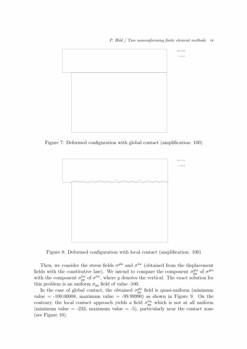
The difference between the solutions of global and local type is considerable. Usingthe same number of inequalities (thirteen) corresponding to the number of nodes of theupper body on the contact zone, the global contact approach yields a very satisfactorysolution in Figure 7 (with an undetectable interpenetration and a straight contactzone) whereas the local contact approach shows a quite unacceptable solution (withan important interpenetration of the bodies) in Figure 8.


AMPLITUDE

1.00E+02

Figure 7: Deformed configuration with global contact (amplification: 100)

AMPLITUDE

1.00E+02

Figure 8: Deformed configuration with local contact (amplification: 100)

Then, we consider the stress fields σglo and σloc (obtained from the displacementfields with the constitutive law). We intend to compare the component σglo

yy of σglo

with the component σlocyy of σloc, where y denotes the vertical. The exact solution for

this problem is an uniform σyy field of value -100.In the case of global contact, the obtained σglo

yy field is quasi-uniform (minimumvalue = -100.00008, maximum value = -99.99990) as shown in Figure 9. On thecontrary, the local contact approach yields a field σloc

yy which is not at all uniform(minimum value = -233, maximum value = -5), particularly near the contact zone(see Figure 10).


GIBI FECIT

VAL − ISO

−100.00009

−100.00008

−100.00007

−100.00006

−100.00005

−100.00004

−100.00003

−100.00002

−100.00001

−100

−99.99999

−99.99998

−99.99997

−99.99996

−99.99995

−99.99994

−99.99993

−99.99992

−99.99991

−99.99990

−99.99989

−99.99988

Figure 9: The σgloyy field obtained with global contact (minimum value = -100.00008,

maximum value = -99.99990)

GIBI FECIT

VAL − ISO

−232

−221

−211

−200

−189

−178

−168

−157

−146

−136

−125

−114

−104

−93

−82

−71

−61

−50

−39

−29

−18

−7

Figure 10: The σlocyy field obtained with local contact (minimum value = -233.77,

maximum value = -5.42)


Finally, Figure 11 shows the Lagrange multipliers equal to (A1)−1Φ0. The massmatrix A1 has been introduced in (4.5) and Φ0 is the solution of the minimizationproblem (4.7) in the global case and of (4.11) in the local case. These multipliers,defined on the contact zone, express the normal stresses (exact value = -100). Onceagain, we notice the quite good value of the global contact multiplier and the impor-tant irregularities of the multiplier obtained when using local contact conditions.

0 0.1 0.2 0.3 0.4 0.5 0.6 0.7 0.8 0.9 1−115

−110

−105

−100

−95

−90

−85

−80

−75

Contact zone

Val

ue o

f the

mul

tiplie

r

Figure 11: Lagrange multipliers corresponding to global (o) and local (x) conditions

If we choose the symmetrical definition of the contact condition (3.3) (see Remark3.1) and the symmetrical definition of the contact condition (3.4), we obtain thedeformed configurations of Figures 12 and 13. In this case, the difference betweenthe global and the local contact conditions is obviously less significant than in theprevious comparison but the global solution remains a bit better.

As in the symmetrical case, we consider the stress fields σglo and σloc. In thecase of global contact, the obtained σglo

yy field is still quasi-uniform (minimum value= -100.0032, maximum value = -99.9965) as shown in Figure 14. Notice that thelocal approach gives a suitable field σloc

yy (minimum value = -101.86, maximum value= -95.935, see Figure 15). Concerning the Lagrange multipliers depicted in Figure16, we can still notice the very good results given by the global approach and thesatisfactory solution yielded by the local conditions.


AMPLITUDE

1.00E+02

Figure 12: Deformed configuration with the symmetrical definition of global contact(amplification: 100)

AMPLITUDE

1.00E+02

Figure 13: Deformed configuration with the symmetrical definition of local contact(amplification: 100)


GIBI FECIT

VAL − ISO

−100.0030

−100.0027

−100.0024

−100.0021

−100.0018

−100.0015

−100.0012

−100.0009

−100.0006

−100.0003

−100

−99.9997

−99.9994

−99.9991

−99.9988

−99.9985

−99.9982

−99.9979

−99.9976

−99.9973

−99.9970

−99.9967

Figure 14: The σgloyy field obtained with the symmetrical definition of global contact

(minimum value = -100.0032, maximum value = -99.9965)

GIBI FECIT

VAL − ISO

−102

−101.7

−101.4

−101.1

−100.8

−100.5

−100.2

−99.9

−99.6

−99.3

−99

−98.7

−98.4

−98.1

−97.8

−97.5

−97.2

−96.9

−96.6

−96.3

−96

−95.7

Figure 15: The σlocyy field obtained with the symmetrical definition of local contact

(minimum value = -101.86, maximum value = -95.935)


0 0.1 0.2 0.3 0.4 0.5 0.6 0.7 0.8 0.9 1−104

−102

−100

−98

−96

−94

−92

Contact zone

Val

ue o

f the

mul

tiplie

r

Figure 16: Lagrange multipliers corresponding to symmetrical global (o) and sym-metrical local (x) conditions

From this test, it becomes manifest that the local contact approach must beavoided, especially when defining the constraints on the coarser grid. Let us re-mark that the meshes have been choosen precisely to show a great difference betweenthe two results. Talking of that, we notice that thirteen inequalities of local type(or of node-on-segment type) describe in a very poor way the contact, whereas thethirteen inequalities of global type are quite representative. This also explains thespectacular superiority of the global contact approach.

When defining the contact conditions on the finer grid, the difference between thetwo approaches is less significant but the global technique still leads to better results.


5.3. Test 3: a case with an initial gap

Figure 17 shows the contact problem between an elastic half-disc and an elasticsupport. The aim of this example is to try to adapt the global contact procedure toa more general context than the previous ones.

Ω

Ω1

2

c c1 2

d d1 2

Figure 17: Reference problem

In such a configuration, we have to consider non-matching meshes, on account ofthe geometries of the bodies. Moreover, there is an initial gap and consequently, thereare points of the boundaries initially not in contact which will come into contact afterdeformation. So, we define the contact by introducing an extended global conditionwhich takes into account of the initial gap (see Remark 4.2). We choose end pointsc1 = (xc1 , yc1), c2 = (xc2 , yc2) on ∂Ω1 and d1 = (xd1

, yd1), d2 = (xd2

, yd2) on ∂Ω2

satisfying xc1 = xd1and xc2 = xd2

. The latter construction is achieved in order tohave a common interface Γc = [d1, d2] where we can project (in the vertical direction)the nodes of the arc of the circle (c1, c2) and define the global contact conditions.

The half-disc is 20 mm in diameter and the length of an edge of the support is40 mm. A Poisson’s ratio of 0.2 for both solids, Young’s modulus E1 = 25000 Mpafor the upper body and E2 = 15000 Mpa for the lower body are assumed. Theapplied loads on the top are 500 daN/mm2.

The initial and the deformed configurations are depicted in Figure 18. Figure 19represents the initial and the deformed meshes near the contact zone, and we observe


a deformed configuration which seems quite satisfactory, particularly on the contactpart.

AMPLITUDE

0.

1.0

Figure 18: The initial and the deformed configuration

AMPLITUDE

0.

1.0

cd

2

2

cd1

1

Figure 19: The initial and the deformed meshes near the contact zone


The contact pressure (given by the Lagrange multiplier) on the arc of the circle(c1, c2) on ∂Ω1 is depicted in Figure 20. By using the generalized load vectors on thenodes of [d1, d2] on ∂Ω2, it becomes possible to obtain the contact pressure on [d1, d2]as shown in Figure 21.

10x 642 8 10,47103

-1

-2

-1.5

-0.5

0

Val

ue o

f th

e m

ultip

lier

c2c1

Figure 20: The contact pressure on the arc of the circle (c1, c2) on ∂Ω1

10x 642 80

3

-1

-2

-1.5

-0.5

0

Con

tact

pre

ssur

e

21d d10

Figure 21: The contact pressure on the segment [d1, d2] on ∂Ω2


5.4. Test 4: taking into account quasi-matching meshes and strong vari-

ations of the contact pressure

The purpose of this last example is to show how the global contact conditionscan take into account quasi-matching meshes and strong variations of the contactpressure.

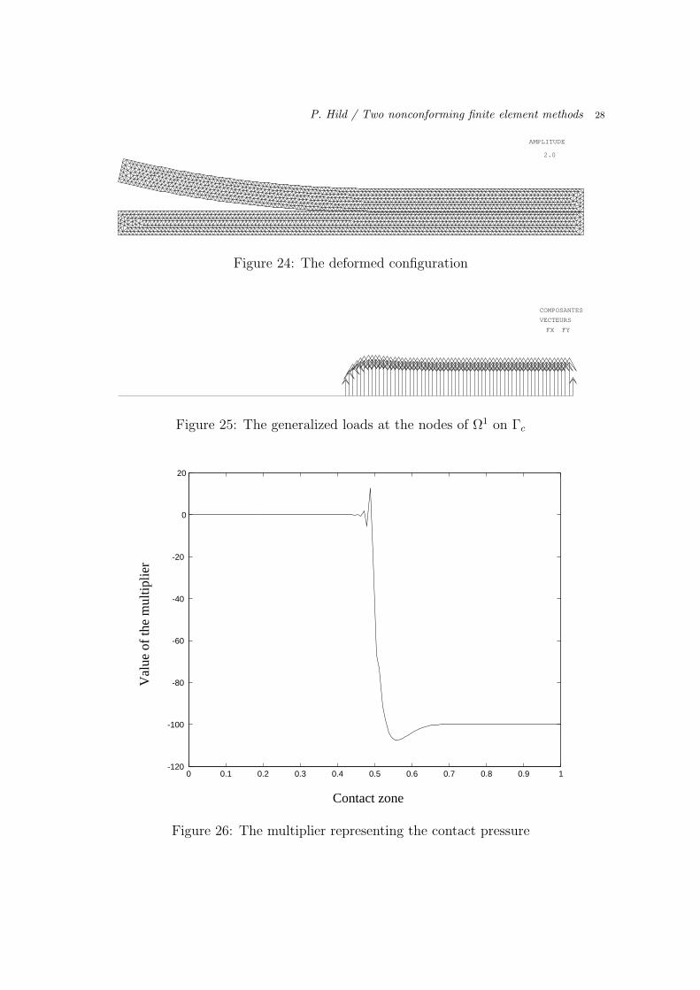
Let us consider the contact problem of Figure 22. The dimensions of Ω1 andΩ2 are 1mm × 0.05mm. A Poisson’s ratio of 0.2 for both solids, Young’s modulusE1 = 25000 Mpa for the upper body and E2 = 15000 Mpa for the lower body areassumed. The applied loads are 100 daN/mm2. The mesh of Ω1 divides Γc into120 identical segments and the mesh of Ω2 divides Γc into 121 identical segmentsas suggested on Figure 23. The deformed meshes are shown on Figure 24 and thegeneralized loads at the nodes of Ω1 on Γc are depicted on Figure 25. Finally, themultiplier, representing the contact pressure is obtained by using the latter loads(see Figure 26). As already noticed in Remark 4.1., the multiplier is not alwaysnonpositive.

As a result, this example shows that the global contact procedure takes into ac-count strong variations of the contact pressure (and meshes which seem difficult tohandle) in a satisfactory way.

ΩΩ

1

2

Figure 22: Setting of the problem

Ω1

Ω2

Figure 23: The meshes (left part of the structure)


AMPLITUDE

2.0

Figure 24: The deformed configuration

COMPOSANTES

VECTEURS

FX FY

Figure 25: The generalized loads at the nodes of Ω1 on Γc

0 0.1 0.2 0.3 0.4 0.5 0.6 0.7 0.8 0.9 1-120

-100

-80

-60

-40

-20

0

20

Val

ue o

f th

e m

ultip

lier

Contact zone

Figure 26: The multiplier representing the contact pressure


6. CONCLUSION AND PERSPECTIVES

In order to solve the unilateral contact problem between two elastic bodies, wehave considered two finite element approximations (one global, one local) of orderone using non–matching meshes on the contact zone.

We have proved that the global approximation extends in an optimal way theresults of Haslinger, Hlavacek and Necas,16, established in the case of matching meshesand we have obtained a convergence result in the case of the local approach. Themethods have been compared and we come to the conclusion that the global approachcould be a promising technique.

For frictional contact, the global contact condition can also be used, and the firsttheoretical studies can be found in 3,18. In other respects, it would be interesting touse other minimization algorithms, in particular Newton like minimization techniques(see 2). Finally, the extension of such a global contact technique to threedimensionalproblems by using the results of 4 is the following study which should be investigated.

Acknowledgments: The author is deeply grateful to P. Laborde and F. BenBelgacem from MIP-Toulouse for their useful advice and contribution. Many thanksto J.-P. Pelle and P. Coorevits from LMT-Cachan for their help in the first numericalexperiments. I am also very thankful to the anonymous referee for the numerousremarks and suggestions which have led to significant improvements of this paper.

References

1. R. A. Adams, Sobolev Spaces, Academic Press, (1975).2. P. Alart, Methode de Newton generalisee en mecanique du contact, J. Math. Pures Appl.,

76, 83–108, (1997).3. G. Bayada, M. Chambat, K. Lhalouani and T. Sassi, Elements finis avec joints pour des

problemes de contact avec frottement de Coulomb non local, C. R. Acad. Sci. Paris,Serie I, 325, 1323–1328, (1997).

4. F. Ben Belgacem, Discretisations 3D non conformes par la methode de decompositionde domaine des elements avec joints : Analyse mathematique et mise en œuvre pour leprobleme de Poisson, These de l’Universite Pierre et Marie Curie, Paris 6, (1993).

5. F. Ben Belgacem, P. Hild and P. Laborde, Approximation of the unilateral contact prob-lem by the mortar finite element method, C. R. Acad. Sci. Paris, Serie I, 324, 123–127,(1997).

6. F. Ben Belgacem, P. Hild and P. Laborde, Extension of the mortar finite element methodto a variational inequality modeling unilateral contact, Math. Mod. and Meth. in the Appl.Sci., 9, No. 2, 287-303, (1999).

7. F. Ben Belgacem, P. Hild and P. Laborde, The mortar finite element method for contactproblems, Math. Comput. Model., 28, 263–271, (1998).

8. C. Bernardi, Y. Maday and A. T. Patera, A new nonconforming approach to domaindecomposition: the mortar element method, College de France Seminar, H. Brezis, J.–L.Lions, Pitman, 13–51, (1994).

9. F. Brezzi, W. W. Hager and P. A. Raviart, Error estimates for the finite element solutionof variational inequalities, Numer. Math., 28, 431–443, (1977).

10. M. D. Canon and C. D. Cullum, A tight upper bound on the rate of convergence of theFrank-Wolfe algorithm, SIAM, Jour. on Control, 6, 509–516, (1968).


11. P.–G. Ciarlet, The finite element method for elliptic problems, North Holland, Amster-dam, (1978).

12. P. Coorevits, P. Hild and J.–P. Pelle, Controle des calculs par elements finis pour unprobleme de contact unilateral, Internal report of LMT-Cachan, IR 203, submitted toRevue Europeenne des Elements Finis, (1998).

13. G. Duvaut and J.–L. Lions, Les inequations en mecanique et en physique, Dunod, Paris,(1972).

14. M. Frank and P. Wolfe, An algorithm for quadratic programming, Naval Research LogistQuarterly, 3, 95–110, (1956).

15. J. Haslinger and I. Hlavacek, Contact between elastic bodies -2. Finite element analysis,Aplikace Matematiky, 26, 263–290, (1981).

16. J. Haslinger, I. Hlavacek and J. Necas, Numerical methods for unilateral problems in solidmechanics, in Handbook of Numerical Analysis, Volume IV, Part 2, Eds. P.G. Ciarletand J.–L. Lions, North Holland, 313–485, (1996).

17. P. Hild, Problemes de contact unilateral et maillages elements finis incompatibles, Thesede l’Universite Paul Sabatier, Toulouse 3, (1998).

18. P. Hild, Elements finis non conformes pour un probleme de contact unilateral avec frot-tement, C. R. Acad. Sci. Paris, Serie I, 324, 707–710, (1997).

19. P. Hild, A propos d’approximation par elements finis optimale pour les problemes decontact unilateral, C. R. Acad. Sci. Paris, Serie I, 326, 1233–1236, (1998).

20. J.–B. Hiriart–Urruty and C. Lemarechal, Convex Analysis and Minimisation Algo-rithms, Volume I and II, in Grundlehren der Mathematischen Wissenschaften (305,306),Springer–Verlag, Berlin, Heidelberg, (1993).

21. N. Kikuchi and J. T. Oden, Contact problems in elasticity: a study of variational inequal-ities and finite element methods, SIAM, Philadelphia, (1988).

22. P. Le Tallec and T. Sassi, Domain decomposition with nonmatching grids: augmentedlagrangian approach, Math. of Comp., 64, 1367–1396, (1995).

23. C. Licht, E. Pratt and M. Raous, Remarks on a numerical method for unilateral contactincluding friction, in International Series of Numerical Mathematics, 101, Birkhauser,129–144, (1991).

24. M. Minoux, Programmation mathematique, theorie et algorithmes, Tome 1, Dunod,(1983).

25. K. Lhalouani and T. Sassi, Nonconforming mixed variational formulation and domaindecomposition for unilateral problems, Internal report of Equipe d’Analyse NumeriqueLyon / Saint-Etienne, IR 286, (1998).

26. P. Wolfe,Convergence theory in nonlinear programming, in Integer and nonlinear pro-gramming, J. Abadie (ed.), North-Holland, Amsterdam 1–36, (1970).

Numerical Implementation of Two Nonconforming Finite ...phild/Publications/CMAME1.pdfNumerical Implementation of Two Nonconforming Finite Element Methods for Unilateral Contact Patrick

Documents