Numerical Hydraulics Wolfgang Kinzelbach with Marc Wolf and Cornel Beffa Lecture 2: Turbulence.

Numerical Hydraulics

Wolfgang Kinzelbach with

Marc Wolf and

Cornel Beffa

Lecture 2: Turbulence

Problems of solving the Navier-Stokes equations

• Analytical solutions only known for simple borderline cases (e.g. laminar pipe flow)

• Equations non-linear (advective acceleration)• Flow becomes turbulent • Direct numerical solution (DNS) today only

possible for relatively low Reynolds numbers• Resolution required for fully developed turbulent

flow: roughly 1/1000 of domain size (i.e. in 3D 109 nodes)

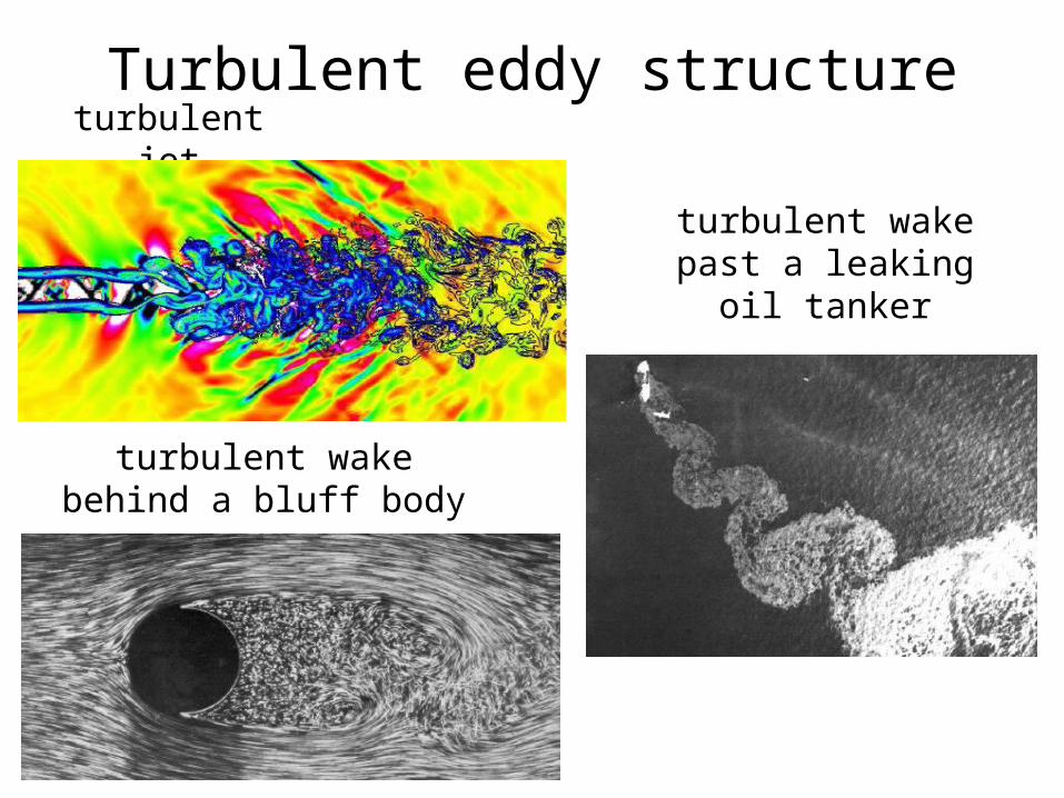
Turbulent eddy structureturbulent jet

turbulent wake behind a bluff body

turbulent wake past a leaking oil tanker

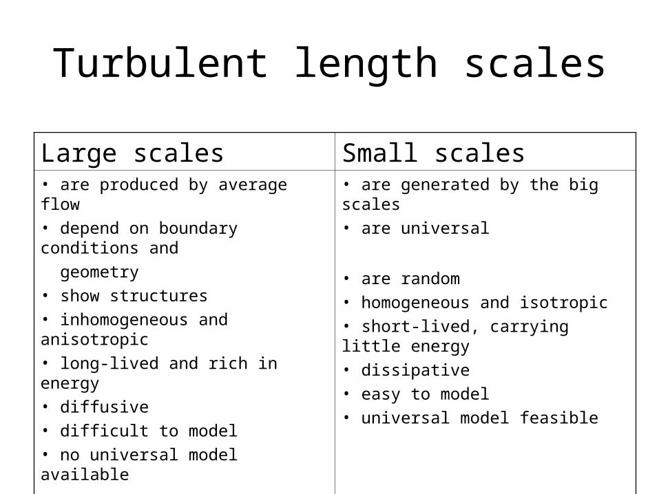
Turbulent length scales

Large scales Small scales• are produced by average flow

• depend on boundary conditions and

geometry

• show structures

• inhomogeneous and anisotropic

• long-lived and rich in energy

• diffusive

• difficult to model

• no universal model available

• are generated by the big scales

• are universal

• are random

• homogeneous and isotropic

• short-lived, carrying little energy

• dissipative

• easy to model

• universal model feasible

Classification of methods

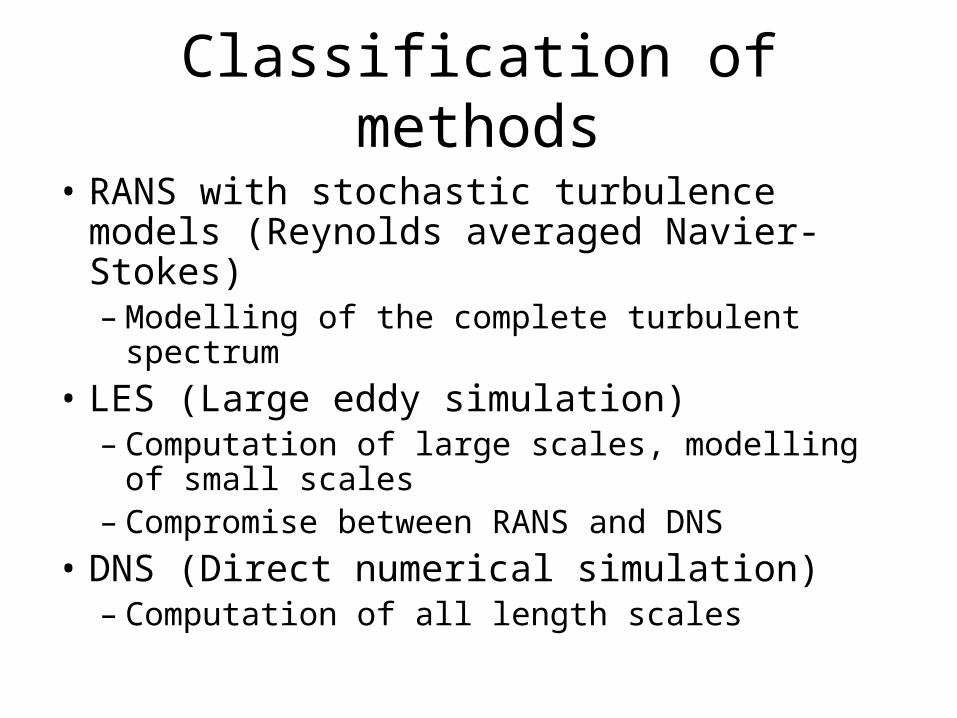
• RANS with stochastic turbulence models (Reynolds averaged Navier-Stokes)– Modelling of the complete turbulent spectrum

• LES (Large eddy simulation) – Computation of large scales, modelling of

small scales– Compromise between RANS and DNS

• DNS (Direct numerical simulation)– Computation of all length scales

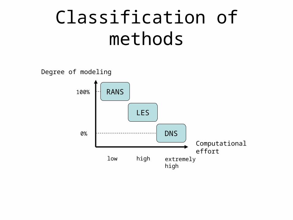
Classification of methods

RANS

LES

DNSComputationaleffort

Degree of modeling

0%

100%

low high extremelyhigh

Strong and weak points of DNS– No closure problem of turbulence, no turbulence

model necessary– Resolution of all characteristic scales necessary– Problem: Ratio of small turbulence elements (lk) in

comparison to large elements (L) grows fast with Re-number: L/lk ~ Re3/4

– Number of grid points NG as well as number of arithmetic operations Nop grow fast with Re: NG ~ Re9/4 , Nop ~ Re11/4

– DNS requires extremely high computer power and storage

– DNS in the foreseeable future limited to small Re (Re<104)

– DNS still great tool for basic research– DNS suitable to produce reference data for validation

of other methods

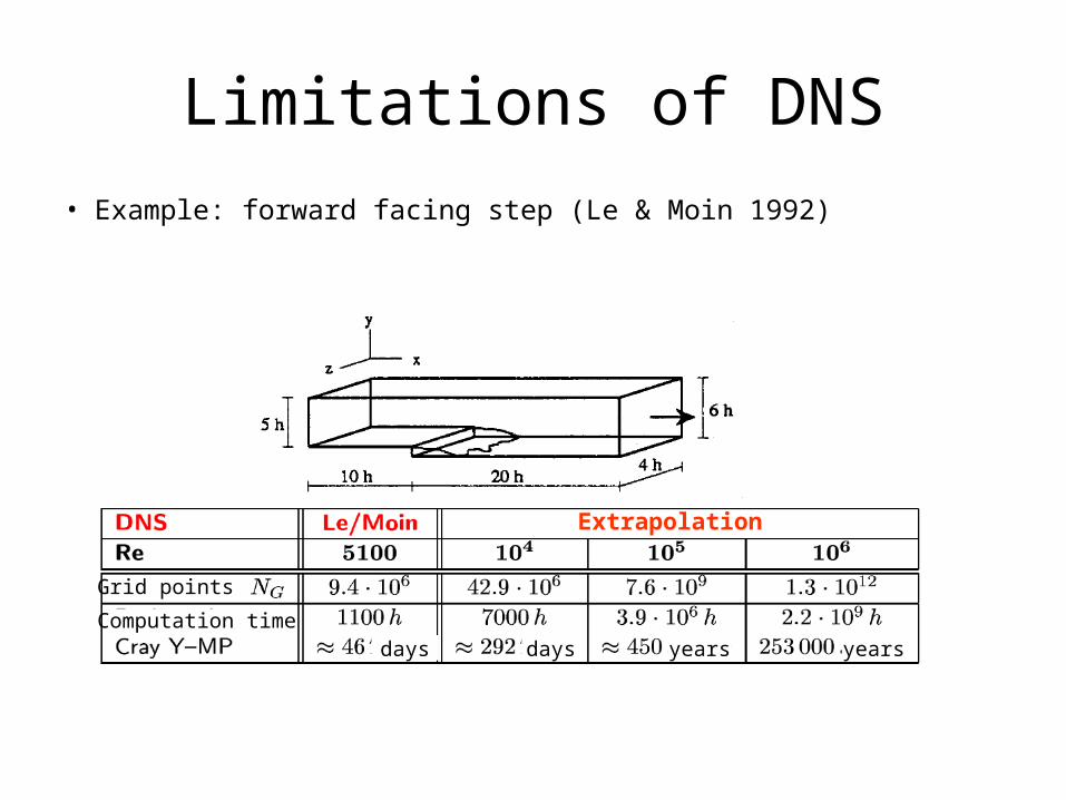
Limitations of DNS

• Example: forward facing step (Le & Moin 1992)

Extrapolation

Grid points

Computation timedays days years years

Reynolds equations (RANS)

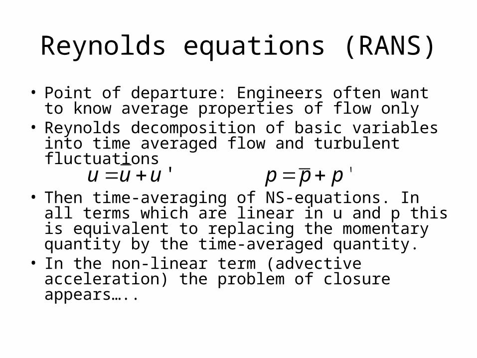
• Point of departure: Engineers often want to know average properties of flow only

• Reynolds decomposition of basic variables into time averaged flow and turbulent fluctuations

• Then time-averaging of NS-equations. In all

terms which are linear in u and p this is equivalent to replacing the momentary quantity by the time-averaged quantity.

• In the non-linear term (advective acceleration) the problem of closure appears…..

' 'u u u p p p

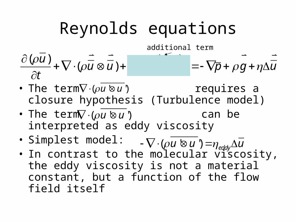
Reynolds equations

• The term requires a closure hypothesis (Turbulence model)

• The term can be interpreted as eddy viscosity

• Simplest model: • In contrast to the molecular viscosity, the eddy

viscosity is not a material constant, but a function of the flow field itself

( )( ) ( ' ')

uu u u u p g u

t( ' ')

u u

( ' ') u u

( ' ') eddyu u u

additional term

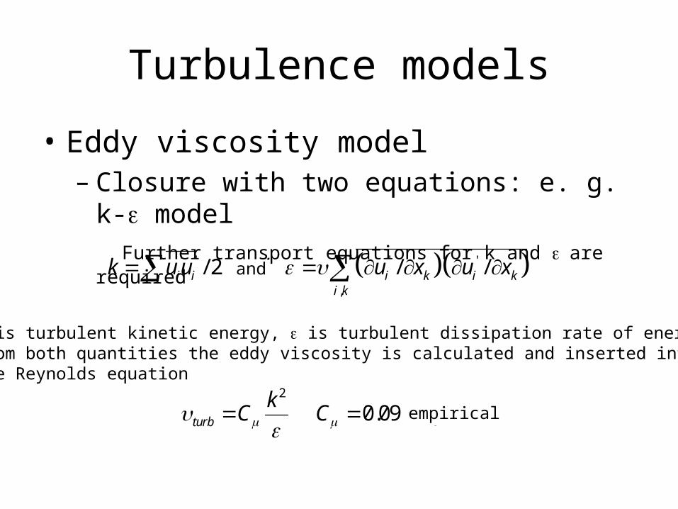
Turbulence models

• Eddy viscosity model– Closure with two equations: e. g. k- model Further transport equations for k and are required

' ' ' '

,

/ 2 / /i i i k i ki k

k u u und u x u x

2

0.09turb

kC C empirisch

k is turbulent kinetic energy, is turbulent dissipation rate of energy From both quantities the eddy viscosity is calculated and inserted intothe Reynolds equation

and

empirical

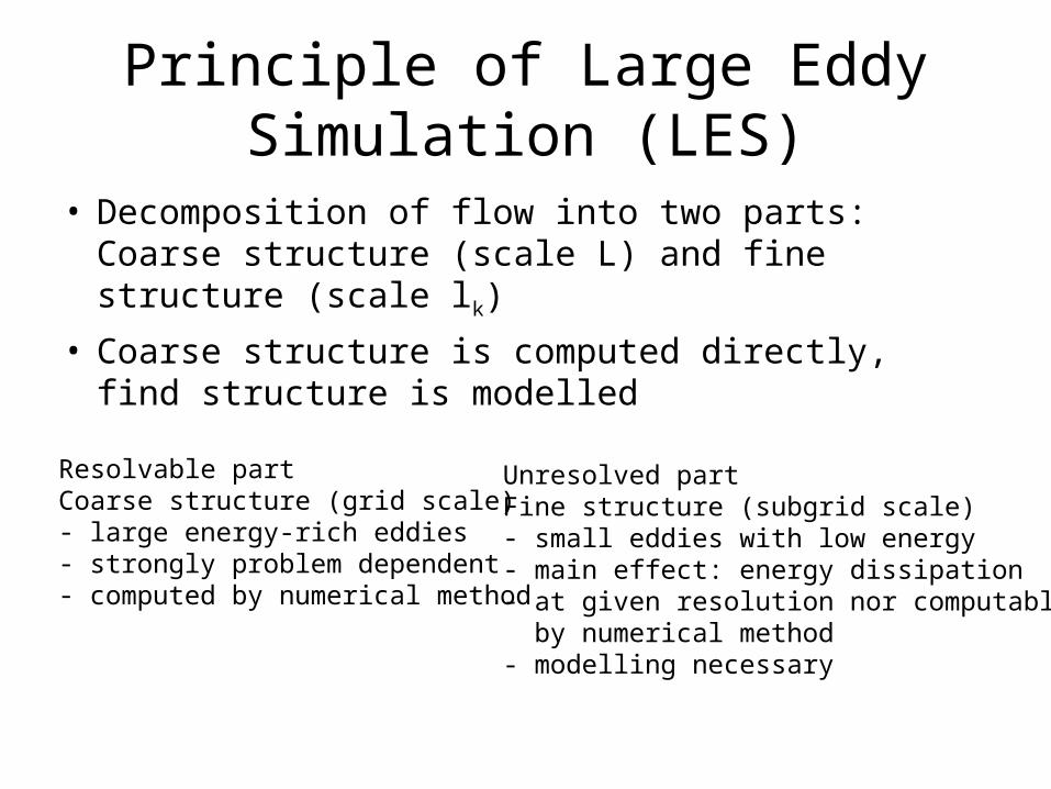
Principle of Large Eddy Simulation (LES)

• Decomposition of flow into two parts: Coarse structure (scale L) and fine structure (scale lk)

• Coarse structure is computed directly, find structure is modelled

Resolvable partCoarse structure (grid scale)- large energy-rich eddies- strongly problem dependent- computed by numerical method

Unresolved partFine structure (subgrid scale)- small eddies with low energy- main effect: energy dissipation- at given resolution nor computable by numerical method- modelling necessary

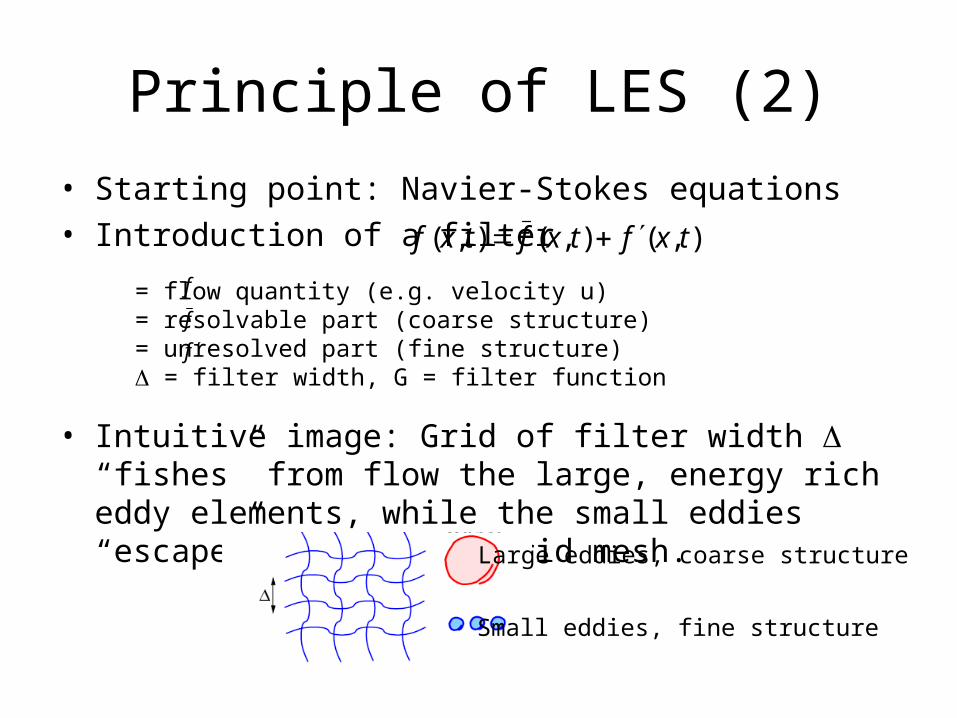
Principle of LES (2)

• Starting point: Navier-Stokes equations• Introduction of a filter

• Intuitive image: Grid of filter width “fishes” from flow the large, energy rich eddy elements, while the small eddies “escape” through the grid mesh.

),(),(),( txftxftxf

= flow quantity (e.g. velocity u)= resolvable part (coarse structure)= unresolved part (fine structure) = filter width, G = filter function

f

f

f

Large eddies, coarse structure

Small eddies, fine structure

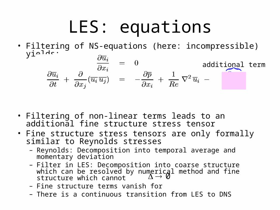
LES: equations• Filtering of NS-equations (here: incompressible) yields:

• Filtering of non-linear terms leads to an additional fine structure stress tensor

• Fine structure stress tensors are only formally similar to Reynolds stresses– Reynolds: Decomposition into temporal average and momentary

deviation– Filter in LES: Decomposition into coarse structure which can be

resolved by numerical method and fine structure which cannot– Fine structure terms vanish for– There is a continuous transition from LES to DNS

0

additional term

LES: fine structure models (1)

• Tasks of the fine structure model– Modelling the influence of turbulent fine structure on the coarse

structure– Modelling the energy transfer between the resolved scales and

the unresolved scales in the correct order of magnitude (fine scales have to extract the right amount of energy from the large scales)

• Classification of fine structure models– Zero equation models (algebr. eddy viscosity models)– One equation models– Two equation models– Etc.

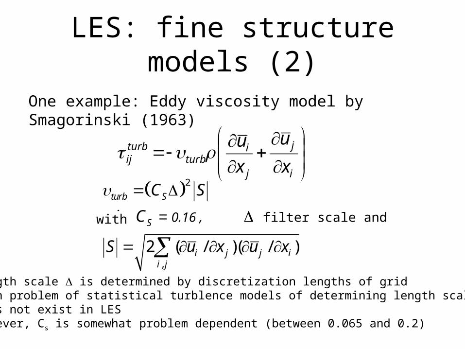
LES: fine structure models (2)

One example: Eddy viscosity model by Smagorinski (1963)

2

,

0.1 0.2,

2 ( / )( / )

turb S

S

i j j ii j

C S

mit C Filterskala und

S u x u x

with filter scale and -

i

j

j

iturb

turbij x

u

x

u

Length scale is determined by discretization lengths of gridMain problem of statistical turblence models of determining length scale ldoes not exist in LESHowever, Cs is somewhat problem dependent (between 0.065 and 0.2)

0.16 ,

Summary LES

• LES is middle way between DNS and RANS• In LES only small scale turbulence has to be modelled• Models are simpler and more universal than in RANS• LES is particularly suited for complex flows with large

scale structures• LES more and more interesting for engineering• Many details still have to be solved (e.g. Boundary

conditions)• Growing computer power makes LES more and more

attractive

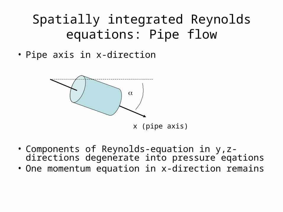
Spatially integrated Reynolds equations: Pipe flow

• Pipe axis in x-direction

• Components of Reynolds-equation in y,z-directions degenerate into pressure eqations

• One momentum equation in x-direction remains

x (pipe axis)

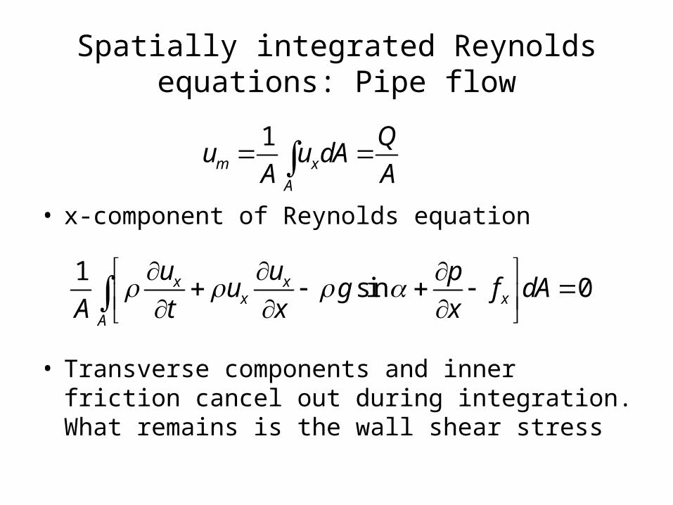
Spatially integrated Reynolds equations: Pipe flow

• x-component of Reynolds equation

• Transverse components and inner friction cancel out during integration. What remains is the wall shear stress

1sin 0x x

x x

A

u u pu g f dA

A t x x

1m x

A

Qu u dA

A A

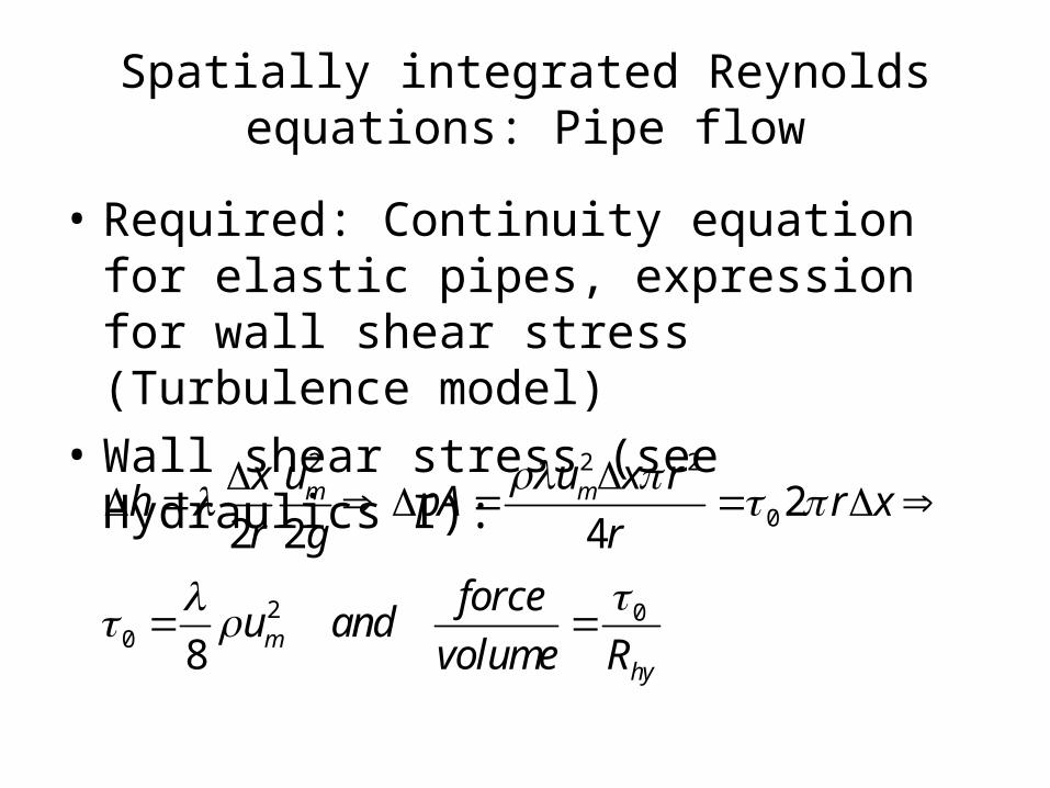
Spatially integrated Reynolds equations: Pipe flow

• Required: Continuity equation for elastic pipes, expression for wall shear stress (Turbulence model)

• Wall shear stress (see Hydraulics I):2 2 2

0

2 00

22 2 4

8

m m

mhy

u u x rxh pA r x

r g r

forceu and

volume R

Spatially integrated Reynolds equations: Pipe flow

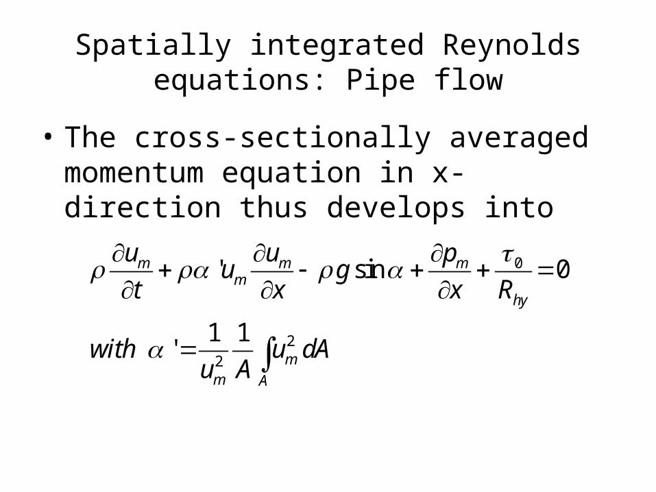
• The cross-sectionally averaged momentum equation in x-direction thus develops into

0

22

' sin 0

1 1'

m m mm

hy

mm A

u u pu g

t x x R

with u dAu A

Spatially integrated Reynolds equations: Pipe flow

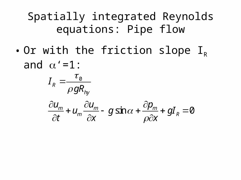
• Or with the friction slope IR and ‘=1:

0

sin 0

Rhy

m m mm R

IgR

u u pu g gI

t x x

Spatially integrated Reynolds equations: Pipe flow

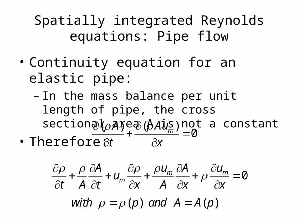
• Continuity equation for an elastic pipe:– In the mass balance per unit length of pipe,

the cross sectional area A is not a constant

• Therefore:( )( )

0mAuA

t x

0m mm

u uA Au

t A t x A x x

( ) ( )with p and A A p

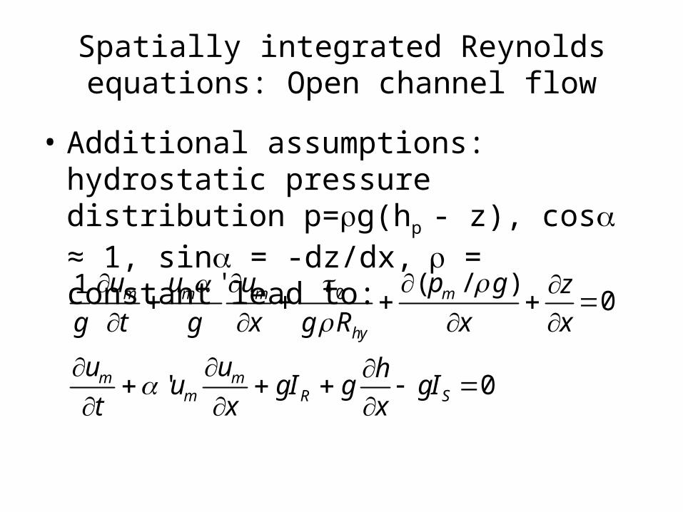
Spatially integrated Reynolds equations: Open channel flow

• Additional assumptions: hydrostatic pressure distribution p=g(hp - z), cos ≈ 1, sin = -dz/dx, = constant lead to:

0' ( / )1

0

' 0

m m m m

hy

m mm R S

u u u p g z

g t g x g R x x

u u hu gI g gI

t x x

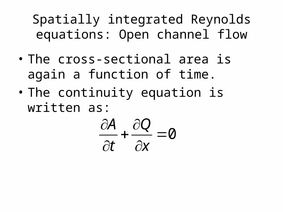
Spatially integrated Reynolds equations: Open channel flow

• The cross-sectional area is again a function of time.

• The continuity equation is written as:

0A Q

t x