Numerical Homogenization of Bone Microstructure

Numerical Homogenization of Bone

Microstructure

Nikola Kosturski and Svetozar Margenov

Institute for Parallel Processing, Bulgarian Academy of Sciences

Abstract. The presented study is motivated by the development ofmethods, algorithms, and software tools for μFE (micro finite element)simulation of human bones. The voxel representation of the bone mi-crostructure is obtained from a high resolution computer tomography(CT) image. The considered numerical homogenization problem con-cerns isotropic linear elasticity models at micro and macro levels.

Keywords: μFEM, nonconforming FEs, homogenization, bonemicrostructure.

1 Introduction

The reference volume element (RVE) of the studied trabecular bone tissue hasa strongly heterogeneous microstructure composed of solid and fluid phases (seeFig. 1). In a number of earlier articles dealing with μFE simulation of bonestructures (see, e.g., [8,10]), the contribution of the fluid phase is neglected. Thissimplification is the starting point for our study and for the related comparativeanalysis. In this study the fluid phase located in the pores of the solid skeleton isconsidered as almost incompressible linear elastic material. This means that thebulk modulus Kf is fixed and the related Poisson ration νf is approaching theincompressibility limit of 0.5. The elasticity modulus Es and the Poisson ratioνs of the solid phase as well as the bulk modulus of the fluid phase Kf are takenfrom [4].

Let Ω ⊂ IR3 be a bounded domain with boundary Γ = ΓD ∪ ΓN = ∂Ω andu = (u1, u2, u3) be the displacements in Ω. The components of the small straintensor are

εij =12

(∂ui

∂xj+

∂uj

∂xi

), 1 ≤ i, j ≤ 3

and the components of the Cauchy stress tensor are

σij = λ

(3∑

k=1

εkk

)δij + 2μεij , 1 ≤ i, j ≤ 3.

Here λ and μ are the Lame coefficients, which can be expressed by the elasticitymodulus E and the Poisson ratio ν ∈ (0, 0.5) as follows

λ =Eν

(1 + ν)(1 − 2ν), μ =

E

2 + 2ν.

I. Lirkov, S. Margenov, and J. Wasniewski (Eds.): LSSC 2009, LNCS 5910, pp. 140–147, 2010.c© Springer-Verlag Berlin Heidelberg 2010

Numerical Homogenization of Bone Microstructure 141

Fig. 1. Microstructure of a trabecular bone specimen

Now, we can introduce the Lame’s system of linear elasticity (see, e.g., [2])

3∑j=1

∂σij

∂xj+ fi = 0, i = 1, 2, 3 (1)

equipped with the boundary conditions

ui(x) = gi(x), x ∈ ΓD ⊂ ∂Ω,3∑

j=1

σij(x)nj(x) = hi(x), x ∈ ΓN ⊂ ∂Ω,

where nj(x) are the components of the normal vector of the boundary for x ∈ΓN .

The remainder of the paper is organized as follows. The applied locking-freenonconforming FEM discretization is presented in the next section. Section 3contains a description of the applied numerical homogenization scheme. Selectednumerical results are given in Section 4. The first test problem illustrates thelocking-free approximation when the Poisson ratio tends to the incompressibilitylimit. Then, a set of numerical homogenization tests for real-life bone microstruc-tures are presented and analyzed. Some concluding remarks are given at the end.

2 Locking-Free Nonconforming FEM Discretization

Let(H1

0 (Ω))3 ={u ∈ (H1(Ω))3 : u = 0 on ΓD

},

(H1g (Ω))3 =

{u ∈ (H1(Ω))3 : u = g on ΓD

}.

The weak formulation of (1) can be written in the form (see, e.g., [3]): for a givenf ∈ (L2(Ω))3 find u ∈ (H1

g (Ω))3 such that for each v ∈ (H10 (Ω))3

a(u,v) = −∫

Ω

(f ,v)dx +∫

ΓN

(h,v)dx.

142 N. Kosturski and S. Margenov

In the case of pure displacement boundary conditions, the bilinear form a(·, ·)can be written as

a(u,v) =∫

Ω

(Cd(u), d(v)) =∫

Ω

(C∗d(u), d(v)) = a∗(u,v), (2)

where

d(u) =(

∂u1

∂x1,∂u1

∂x2,∂u1

∂x3,∂u2

∂x1,∂u2

∂x2,∂u2

∂x3,∂u3

∂x1,∂u3

∂x2,∂u3

∂x3

)T

and the matrices C and C∗ are

C =

⎡⎢⎢⎢⎢⎢⎢⎢⎢⎢⎢⎢⎢⎣

λ + 2μ 0 0 0 λ 0 0 0 λ0 μ 0 μ 0 0 0 0 00 0 μ 0 0 0 μ 0 00 μ 0 μ 0 0 0 0 0λ 0 0 0 λ + 2μ 0 0 0 λ0 0 0 0 0 μ 0 μ 00 0 μ 0 0 0 μ 0 00 0 0 0 0 μ 0 μ 0λ 0 0 0 λ 0 0 0 λ + 2μ

⎤⎥⎥⎥⎥⎥⎥⎥⎥⎥⎥⎥⎥⎦

,

C∗ =

⎡⎢⎢⎢⎢⎢⎢⎢⎢⎢⎢⎢⎢⎣

λ + 2μ 0 0 0 λ + μ 0 0 0 λ + μ0 μ 0 0 0 0 0 0 00 0 μ 0 0 0 0 0 00 0 0 μ 0 0 0 0 0

λ + μ 0 0 0 λ + 2μ 0 0 0 λ + μ0 0 0 0 0 μ 0 0 00 0 0 0 0 0 μ 0 00 0 0 0 0 0 0 μ 0

λ + μ 0 0 0 λ + μ 0 0 0 λ + 2μ

⎤⎥⎥⎥⎥⎥⎥⎥⎥⎥⎥⎥⎥⎦

.

Let us note, that the modified bilinear form a∗(·, ·) is equivalent to a(·, ·) if∫Ω

∂ui

∂xj

∂uj

∂xidx =

∫Ω

∂ui

∂xi

∂uj

∂xjdx (3)

is fulfilled. It is also important, that the rotations are excluded from the kernelof the modified (corresponding to a∗(·, ·)) Neumann boundary conditions oper-ator. As a result, the nonconforming Crouzeix-Raviart (C.–R.) FEs are applica-ble to the modified variational problem, providing a locking-free discretization.Locking-free error estimates of the 2D pure displacement problem discretized byC.–R. FEs are presented, e.g., in [3]. A similar analysis is applicable to the 3Dcase as well.

It is easy to check that the equality (3) holds true also for the RVE withDirichlet boundary conditions with respect to the normal displacements only. Aswe will see in the next section, this is exactly the case in the studied numericalhomogenization scheme.


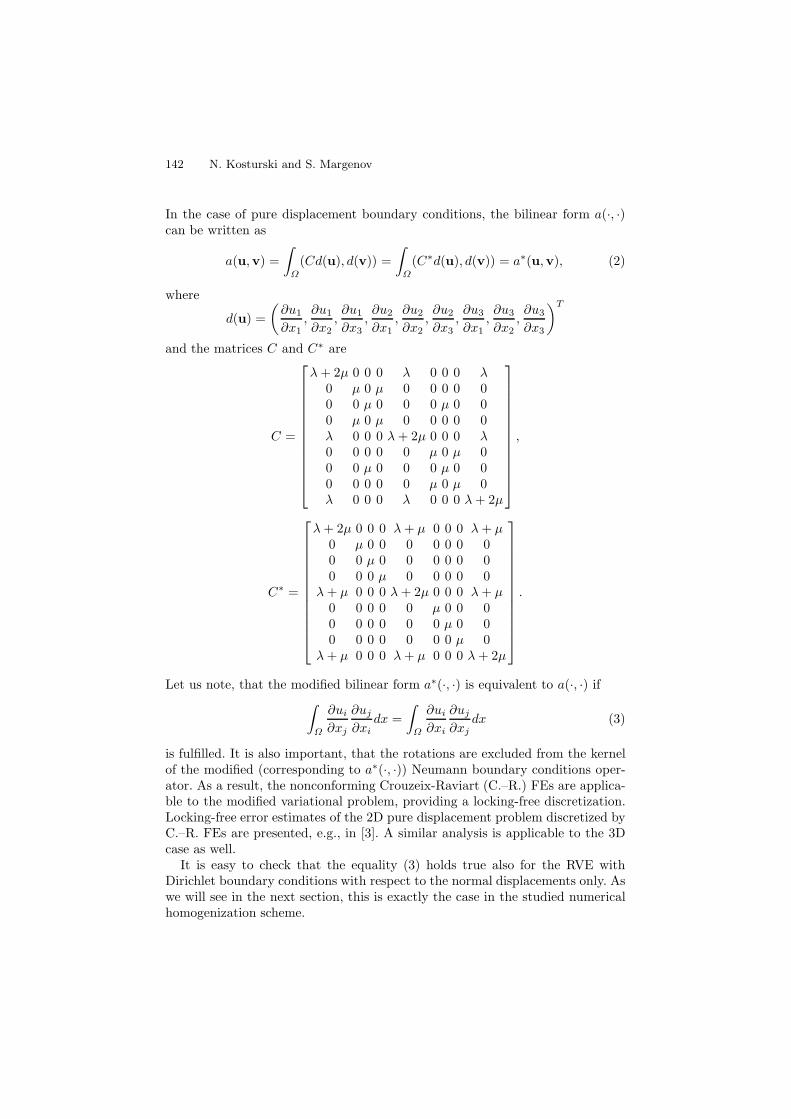
Fig. 2. Splitting a voxel into six tetrahedra

In order to apply C.–R. FE discretization of RVE, we split each voxel(macroelement) into six tetrahedra, see Fig. 2. For a RVE divided into n×n×nvoxels, the number of unknowns in the resulting linear system is 18n2(2n + 1).A block factorization (static condensation) is applied first on the macroelementlevel, eliminating the unknowns associated with the inner nodes. This stepreduces the total number of unknowns to 18n2(n + 1).

3 Numerical Homogenization

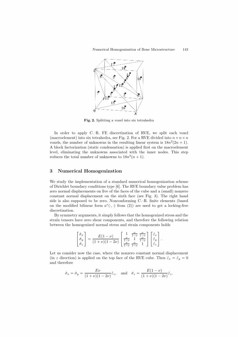
We study the implementation of a standard numerical homogenization schemeof Dirichlet boundary conditions type [6]. The RVE boundary value problem haszero normal displacements on five of the faces of the cube and a (small) nonzeroconstant normal displacement on the sixth face (see Fig. 3). The right handside is also supposed to be zero. Nonconforming C.–R. finite elements (basedon the modified bilinear form a∗(·, ·) from (2)) are used to get a locking-freediscretization.

By symmetry arguments, it simply follows that the homogenized stress and thestrain tensors have zero shear components, and therefore the following relationbetween the homogenized normal stress and strain components holds

⎡⎣ σx

σy

σz

⎤⎦ =

E(1 − ν)(1 + ν)(1 − 2ν)

⎡⎣ 1 ν

1−νν

1−νν

1−ν 1 ν1−ν

ν1−ν

ν1−ν 1

⎤⎦⎡⎣ εx

εy

εz

⎤⎦ .

Let us consider now the case, where the nonzero constant normal displacement(in z direction) is applied on the top face of the RVE cube. Then εx = εy = 0and therefore

σx = σy =Eν

(1 + ν)(1 − 2ν)εz, and σz =

E(1 − ν)(1 + ν)(1 − 2ν)

εz.


Fig. 3. Boundary conditions of the RVE problem

From these relations we can directly calculate the homogenized elasticity co-efficients as follows

ν =1

1 + p, E =

(1 + ν)(1 − 2ν)1 − ν

r,

wherep =

σz

σx=

σz

σy, r =

σz

εz.

In theory σx = σy. In the case of numerical homogenization, the average valuesof the stresses σx and σy over all tetrahedral finite elements are used. In thecase of numerical homogenization of strongly heterogeneous materials (like bonetissues), the average stresses σx and σy are not equal. This is why we set

σx = σy =12

(1

Nel

Nel∑i=1

σix +

1Nel

Nel∑i=1

σiy

)

when computing the homogenized elasticity modulus and Poisson ratio.Similar relations hold when the nonzero displacements are alternatively ap-

plied in the x and y directions. To determine the elasticity coefficients moreprecisely, we apply the above numerical scheme in all three cases, and finallyaverage the computed elasticity modulus and Poisson ratio.

4 Numerical Experiments

A set of numerical tests illustrating the accuracy of the locking-free FEM ap-proximation in the almost incompressible case are presented first. The secondpart of the section contains results of numerical homogenization of three real-life


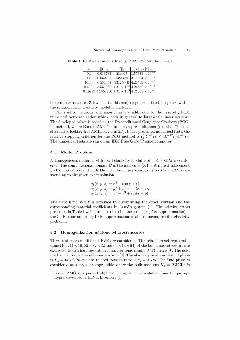
Table 1. Relative error on a fixed 32 × 32 × 32 mesh for ν → 0.5

ν ‖r‖∞ ‖f‖∞ ‖r‖∞/‖f‖∞0.4 0.033733 214407 1.57331 × 10−7

0.49 0.052206 1381450 3.77904 × 10−8

0.499 0.551943 13125600 4.20509 × 10−8

0.4999 5.551980 1.31 × 108 4.24652 × 10−8

0.49999 55.552900 1.31 × 109 4.25009 × 10−8

bone microstructure RVEs. The (additional) response of the fluid phase withinthe studied linear elasticity model is analyzed.

The studied methods and algorithms are addressed to the case of μFEMnumerical homogenization which leads in general to large-scale linear systems.The developed solver is based on the Preconditioned Conjugate Gradient (PCG)[1] method, where BoomerAMG1 is used as a preconditioner (see also [7] for analternative locking-free AMLI solver in 2D). In the presented numerical tests, therelative stopping criterion for the PCG method is rT

k C−1rk ≤ 10−12rT0 C−1r0.

The numerical tests are run on an IBM Blue Gene/P supercomputer.

4.1 Model Problem

A homogeneous material with fixed elasticity modulus E = 0.06 GPa is consid-ered. The computational domain Ω is the unit cube [0, 1]3. A pure displacementproblem is considered with Dirichlet boundary conditions on ΓD = ∂Ω corre-sponding to the given exact solution

u1(x, y, z) = x3 + sin(y + z),u2(x, y, z) = y3 + z2 − sin(x − z),u3(x, y, z) = x2 + z3 + sin(x − y).

The right hand side f is obtained by substituting the exact solution and thecorresponding material coefficients in Lame’s system (1). The relative errorspresented in Table 1 well illustrate the robustness (locking-free approximation) ofthe C.–R. nonconforming FEM approximation of almost incompressible elasticityproblems.

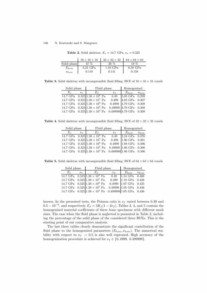
4.2 Homogenization of Bone Microstructures

Three test cases of different RVE are considered. The related voxel representa-tions (16×16×16, 32×32×32 and 64×64×64) of the bone microstructure areextracted from a high resolution computer tomography (CT) image [9]. The usedmechanical properties of bones are from [4]. The elasticity modulus of solid phaseis Es = 14.7 GPa and the related Poisson ratio is νs = 0.325. The fluid phase isconsidered as almost incompressible where the bulk modulus Kf = 2.3 GPa is

1 BoomerAMG is a parallel algebraic multigrid implementation from the packageHypre, developed in LLNL, Livermore [5].


Table 2. Solid skeleton: Es = 14.7 GPa, νs = 0.325

16 × 16 × 16 32 × 32 × 32 64 × 64 × 64

Solid phase 47 % 26 % 19 %

Ehom 3.21 GPa 1.10 GPa 0.58 GPaνhom 0.118 0.141 0.158

Table 3. Solid skeleton with incompressible fluid filling: RVE of 16 × 16 × 16 voxels

Solid phase Fluid phase Homogenized

Es νs Ef νf Ehom νhom

14.7 GPa 0.325 1.38 × 108 Pa 0.49 5.05 GPa 0.29914.7 GPa 0.325 1.38 × 107 Pa 0.499 4.82 GPa 0.30714.7 GPa 0.325 1.38 × 106 Pa 0.4999 4.79 GPa 0.30914.7 GPa 0.325 1.38 × 105 Pa 0.49999 4.79 GPa 0.30914.7 GPa 0.325 1.38 × 104 Pa 0.499999 4.79 GPa 0.309









known. In the presented tests, the Poisson ratio is νf varied between 0.49 and0.5 − 10−6, and respectively Ef = 3Kf(1 − 2νf ). Tables 3, 4, and 5 contain thehomogenized material coefficients of three bone specimens with different meshsizes. The case when the fluid phase is neglected is presented in Table 2, includ-ing the percentage of the solid phase of the considered three RVEs. This is thestarting point of our comparative analysis.

The last three tables clearly demonstrate the significant contribution of thefluid phase to the homogenized parameters (Ehom, νhom). The numerical sta-bility with respect to νf → 0.5 is also well expressed. High accuracy of thehomogenization procedure is achieved for νf ∈ {0, 4999, 0.499999}.


The following next steps in the numerical homogenization of bone microstruc-tures are planned: a) anisotropic macro model; b) poroelasticity micro model.The goal is to improve further (quantitatively and qualitatively) our understand-ing of the underlying phenomena.

Acknowledgments

This work is partly supported by the Bulgarian NSF Grants DO02-115/08 andDO02-147/08. We kindly acknowledge also the support of the Bulgarian Super-computing Center for the access to the supercomputer IBM Blue Gene/P.

References

1. Axelsson, O.: Iterative solution methods. Cambridge University Press, Cambridge(1994)

2. Axelsson, O., Gustafsson, I.: Iterative methods for the Navier equations of elastic-ity. Comp. Meth. Appl. Mech. Engin. 15, 241–258 (1978)

3. Brenner, S., Sung, L.: Nonconforming finite element methods for the equations oflinear elasticity. Math. Comp. 57, 529–550 (1991)

4. Cowin, S.: Bone poroelasticity. J. Biomechanics 32, 217–238 (1999)5. Lawrence Livermore National Laborary, Scalable Linear Solvers Project,

https://computation.llnl.gov/casc/linear_solvers/sls_hypre.html

6. Kohut, R.: The determination of Young modulus E and Poisson number ν of geo-composite material using mathematical modelling, private communication (2008)

7. Kolev, T., Margenov, S.: Two-level preconditioning of pure displacement non-conforming FEM systems. Numer. Lin. Algeb. Appl. 6, 533–555 (1999)

8. Margenov, S., Vutov, Y.: Preconditioning of Voxel FEM Elliptic Systems. TASK,Quaterly 11(1-2), 117–128 (2007)

9. Vertebral Body Data Set ESA29-99-L3,http://bone3d.zib.de/data/2005/ESA29-99-L3

10. Wirth, A., Flaig, C., Mueller, T., Muller, R., Arbenz, P., van Lenthe, G.H.:Fast Smooth-surface micro-Finite Element Analysis of large-scale bone models.J. Biomechanics 41 (2008), doi:10.1016/S0021-9290(08)70100-3

https://computation.llnl.gov/casc/linear_solvers/sls_hypre.html

http://bone3d.zib.de/data/2005/ESA29-99-L3

Numerical Homogenization of Bone Microstructure

Documents