© 2013. Sharaban Thohura & Azad Rahman. This is a research/review paper, distributed under the terms of the Creative Commons Attribution-Noncommercial 3.0 Unported License http://creativecommons.org/licenses/by-nc/3.0/), permitting all non commercial use, distribution, and reproduction in any medium, provided the original work is properly cited. Global Journal of Science Frontier Research Mathematics and Decision Sciences Volume 13 Issue 6 Version 1.0 Year 2013 Type : Double Blind Peer Reviewed International Research Journal Publisher: Global Journals Inc. (USA) Online ISSN: 2249-4626 & Print ISSN: 0975-5896 Numerical Approach for Solving Stiff Differential Equations: A Comparative Study By Sharaban Thohura & Azad Rahman Jagannath University, Bangladesh Abstract - In this paper our attention is directed towards the discussion of phenomenon of stiffness and towards general purpose procedures for the solution of stiff differential equations. Our aim is to identify the problem area and the characteristics of the stiff differential equations for which the equations are distinguishable. Most realistic stiff systems do not have analytical solutions so that a numerical procedure must be used. Computer implementation of such algorithms is widely available e.g. DIFSUB, GEAR, EPISODE etc. The most popular methods for the solution of stiff initial value problems for ordinary differential equations are the backward differentiation formulae (BDFs). In this study we focus on a particularly efficient algorithm which is named as EPISODE, based on variable coefficient backward differentiation formula. Through this study we find that though the method is very efficient it has certain problem area for a new user. All those problem area have been detected and recommended for further modification. GJSFR-F Classification : MSC 2010: 12H20 NumericalApproachforSolvingStiffDifferentialEquations AComparativeStudy Strictly as per the compliance and regulations of :

Welcome message from author
This document is posted to help you gain knowledge. Please leave a comment to let me know what you think about it! Share it to your friends and learn new things together.
Transcript
© 2013. Sharaban Thohura & Azad Rahman. This is a research/review paper, distributed under the terms of the Creative Commons Attribution-Noncommercial 3.0 Unported License http://creativecommons.org/licenses/by-nc/3.0/), permitting all non commercial use, distribution, and reproduction in any medium, provided the original work is properly cited.
Global Journal of Science Frontier Research Mathematics and Decision Sciences Volume 13 Issue 6 Version 1.0 Year 2013 Type : Double Blind Peer Reviewed International Research Journal Publisher: Global Journals Inc. (USA) Online ISSN: 2249-4626 & Print ISSN: 0975-5896
Numerical Approach for Solving Stiff Differential Equations: A Comparative Study
By Sharaban Thohura & Azad Rahman Jagannath University, Bangladesh
Abstract - In this paper our attention is directed towards the discussion of phenomenon of stiffness and towards general purpose procedures for the solution of stiff differential equations. Our aim is to identify the problem area and the characteristics of the stiff differential equations for which the equations are distinguishable. Most realistic stiff systems do not have analytical solutions so that a numerical procedure must be used. Computer implementation of such
algorithms is widely available e.g. DIFSUB, GEAR, EPISODE etc. The most popular methods for the solution of stiff initial value problems for ordinary differential equations are the backward differentiation formulae (BDFs). In this study we focus on a particularly efficient algorithm which is named as EPISODE, based on variable coefficient backward differentiation formula. Through this study we find that though the method is very efficient it has certain problem area for a new user. All those problem area have been detected and recommended for further modification.
GJSFR-F Classification : MSC 2010: 12H20
Numerical Approach for Solving Stiff Differential Equations A Comparative Study
Strictly as per the compliance and regulations of :
Numerical Approach for Solving Stiff
Differential Equations: A Comparative Study Sharaban Thohura
α
& Azad Rahman
σ
Abstract
-
In this paper our attention is directed towards the discussion of phenomenon of stiffness and towards
general purpose procedures for the solution of stiff differential equations. Our aim is to identify the problem area and the
characteristics of the stiff differential equations for which the equations are distinguishable. Most realistic stiff systems do not have analytical solutions so that a numerical procedure must be used. Computer implementation of such
algorithms is widely available e.g. DIFSUB, GEAR, EPISODE etc. The most popular methods for the solution of stiff initial
value problems for ordinary differential equations are the backward differentiation formulae (BDFs). In this study we
focus on a particularly efficient algorithm which is named as EPISODE, based on variable coefficient backward
differentiation formula. Through this study we find that though the method is very efficient it has certain problem area for
a new user. All those problem area have been detected and recommended for further modification.
A very important special class of differential equations
taken up in the initial value
problems termed
as stiff differential equations result from the phenomena with widely
differing time scales. There is no universally accepted definition of stiffness.Stiffness is a
subtle, difficult and important concept in the numerical solution of ordinary differential
equations. It depends on the differential equation, the initial condition and the interval
under consideration.
A set of differential equations is “stiff”
when an excessively small step is needed to
obtain correct integration. In other words we can say a set of differential equations is
“stiff” when it contains at least two “time constants”
(where time is supposed
to be the
joint independent variable) that differ by several orders of magnitude. A more rigorous
definition of stiffness was also given by Shampine and Gear: “By a stiff problem we mean
one for which no solution component is unstable (no eigenvalue of the Jacobian matrix
has a real part which is at all large and positive) and at least some component is very
stable (at least one eigenvalue has a real part which is large and negative). Further, we
7
Globa
lJo
urna
lof
Scienc
eFr
ontie
rResea
rch
V
olum
eXIII
Issue
e
rsion
IV
VI
Yea
r
2 013
F)
)
© 2013 Global Journals Inc. (US)
The initial value problems with stiff ordinary differential equation systems occur in many fields of engineering science, particularly in the studies of electrical circuits, vibrations, chemical reactions and so on. Stiff differential equations are ubiquitous in astrochemical kinetics, many control systems and electronics, but also in many non-industrial areas like weather prediction and biology.
Author α : Assistant Professor, Department of Mathematics, Jagannath University Dhaka-1100, Bangladesh.
E-mail : [email protected]
E-mail : [email protected]
Notes
Author σ : School of Engineering & Technology, Central Queensland University, Australia.
When solving the (vector) system of equations
),,( ytfy aty )( 0 (given) (1)
we must consider the behavior of solutions near to the one we seek. This is because as we
step along from )( nn xyy to 1ny approximating )( hxy n we make inevitable errors
causing us to move from the desired integral curve to a nearby one. If we make no further
errors, we follow this new curve so that the resulting error depends on the relative
behavior of the two solution curves. Let us consider the example of the single equation
),())(( tptpyAy aty o )( (2)
where A is constant. The analytical solution is
)()exp())0(()( tpAtpaty (3)
If A is large and positive, the solution curves for the various a fan out and we say
the problem is unstable. Such a problem, obviously, is difficult for any general numerical
method, which proceeds in a step-by-step fashion. When A is small in magnitude, the
curves are more or less parallel and such neutrally stable problems are easily handled by
conventional means. When A is large and negative, the solution curves converge very
quickly. In fact, whatever be the value of )( oty , the solution curve is virtually identical to
the particular solution p(t) after a short distance called an initial transient. This super-
stable situation is ideal for the propagation of error in a numerical scheme. The last class
of problems is called stiff.
If A is very negative and p (t) is slowly varying, equation (3) represents a stiff
problem after the transient Ate has died out (that is, Ate is below the error tolerance of
interest) but it is not be stiff in the transient region. If (1) is linear with a constant
Jacobian J (where J = ∂f /∂y is the associated Jacobian matrix), it will not be stiff in the
initial transient, but will be stiff after the fastest transient has died out. We see that in
case of stiff differential equation problem the solution being sought is varying slowly, but
there are nearby solutions that vary rapidly, so the numerical method must take small
steps to obtain satisfactory results. Stiffness is an efficiency issue. If we were not
concerned with how much time a computation takes, we would not be concerned about
stiffness. Nonstiff methods can solve stiff problems, but take a long time to do it.
As stiff differential equations occur in many branches of engineering and science, it
is required to solve efficiently. Most realistic stiff systems do not have analytical solutions
so that a numerical procedure must be used. Conventional methods such as Euler, explicit
Runge-Kutta and Adams –Moulton are restricted to a very small step size in order to that
the solution be stable. This means that a great deal of computer time could be required.
In a number of areas, particularly in chemical applications one often encounters
systems of ordinary differential equations which, although mathematically well
conditioned, are virtually impossible to solve with traditional numerical methods because
8
Globa
lJo
urna
lof
Scienc
eFr
ontie
rResea
rch
V
olum
eXIII
Issue
e
rsion
IV
VI
Yea
r
2013
F
)
)
© 2013 Global Journals Inc. (US)
will not call a problem stiff unless its solution is slowly varying with respect to most
negative part of the eigenvalues. Consequently a problem may be stiff for some intervals
and not for others.”
Notes
of the severe step
size constraint imposed by numerical stability. These stiff equations can
be characterized by the presence of transient components which, although negligible
relative to the numerical solution, constrain the step size of traditional numerical methods
to be of the order of the smallest time constant of the problem.
Over the last three decades, there has been significant progress in the development
of numerical stiff ODE solvers both in the areas of ODE solution algorithms and the
associated linear algebra. Consequently, a wide variety of very efficient and reliable ODE
solvers have been developed. In order to take full advantage of the available state-of-the-
art solvers, and to handle computationally demanding various models
in the different field
both accurately and efficiently, a great deal of understanding is required for the
formulation of the problem. The numerical solution algorithm of a standard stiff ODE
solver package comprises two major components: one is the numerical solution method for
the systems of ODEs and the other is for the solution of the resulting linear algebraic
system that arises due to the ODEs solution technique. The structure of the resulting
matrix associated with the linear system has significant computational consequence.
To better understand the advanced ODE solvers and their differences, we first
need to briefly consider the solution methods underlying stiff systems of ODEs and their
corresponding linear algebra. For the solution of a system of ODEs of size N of the form
(1) and a given initial condition, y (t0) = a, some classes of multistep methods are
generally used. To advance the solution in time t from one mesh point to the next,
considering a discrete time mesh ......,........, 10 nttt , multistep methods make use of several
past values of the variable y and its rate of change f with respect to time t (i.e. the past
values of the abundances and the rate equations). The general form of a k-step multistep
method is
k
i
k
iiniini h
0 0fy (4)
where αi
and βi
are constants depending on the order the method, h is the step size in
time and n denotes the mesh number. The well-known Adams methods which use mostly
the past values of f,
k
iininn h
01 fyy
(5)
are the best-known multistep methods for solving nonstiff problems. Each step requires
the solution of a nonlinear system and often a simple functional iteration with an initial
guess, or predictor estimate, is used to advance the integration, which is terminated by a
convergence test. For stiff problems, where sudden changes in the variables can occur (i.e.
there are strong dependencies of the rate equations f upon abundances y in small time
intervals say), simple iteration leads to unacceptable restriction of the step size and
functional iteration fails to converge. Thus, stiffness forces the use of implicit methods
with infinite stability regions when there is no restriction on the step size. The backward
difference formulae (BDF) methods with unbounded region of absolute stability were the
first numerical methods to be proposed for solving stiff ODEs (Curtiss and Hirschfelder,
1952). The BDF used in ODE solvers, are of the general form
9
Globa
lJo
urna
lof
Scienc
eFr
ontie
rResea
rch
V
olum
eXIII
Issue
e
rsion
IV
VI
Yea
r
2 013
F)
)
Notes
© 2013 Global Journals Inc. (US)
nk
iinin h fyy 0
0
(6)
where αi and β0 are coefficients of k th order, k-step BDF methods. As mentioned earlier, a
simple functional iteration will usually fail to converge when problems are stiff and some
form of Newton iteration is usually used for the solution of the resulting nonlinear system.
The Newton iteration involves the solution of an N ×N matrix, P,
P ≈ I − hβ0 J, (7)
where J = ∂ f /∂y is the associated Jacobian matrix, I is an N ×N identity matrix. The
solution to this linear algebraic system contributes significantly to the total computational
time for the solution of stiff problems, as well as affecting the accuracy of the solution
(and hence, also affecting the computational time). For stiff problems the ODE solvers use
a modified Newton iteration that allows time saving strategies for the computation,
storage and the use of the Jacobian matrix. When solving a linear algebraic system, there
are generally two classes of solution methods, direct methods and iterative methods. The
most common direct method used to solve linear systems is the Gaussian elimination
method based on factorization of the matrix in lower and upper triangular factors. The
GEAR, LSODE and VODE solvers all use such a method for the solution of the resulting
linear system. The simplest iterative scheme used to solve linear systems is the Jacobi
iteration, although the more sophisticated iterative solution methods of Krylov subspace
methods, based on a sequence of orthogonal vectors and matrix-vector multiplications,
have been widely used in practical applications such as computational fluid dynamics
(Saad, 2003a). The ODE solvers, LSODPK and VODPK implement Preconditioned
Krylov iterative techniques for the solution of the resulting linear system.
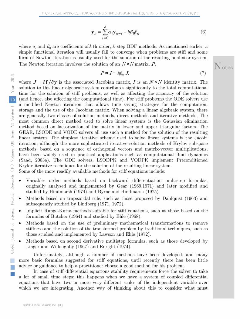
Some of the more readily available methods for stiff equations include:
Variable- order methods based on backward differentiation multistep formulas,
originally analysed and implemented by Gear (1969,1971) and later modified and
studied by Hindmarsh (1974) and Byrne and Hindmarsh (1975).
Methods based on trapezoidal rule, such as those proposed by Dahlquist (1963) and
subsequently studied by Lindberg (1971, 1972).
Implicit Runge-Kutta methods suitable for stiff equations, such as those based on the
formulas of Butcher (1964) and studied by Ehle (1968).
Methods based on the use of preliminary mathematical transformations to remove
stiffness and the solution of the transformed problem by traditional techniques, such as
those studied and implemented by Lawson and Ehle (1972).
Methods based on second derivative multistep formulas, such as those developed by
Linger and Willoughby (1967) and Enright (1974).
Unfortunately, although a number of methods have been developed, and many
more basic formulas suggested for stiff equations, until recently there has been little
advice or guidance to help a practitioner choose a good method for his problem.
In case of stiff differential equations stability requirements force the solver to take
a lot of small time steps; this happens when we have a system of coupled differential
equations that have two or more very different scales of the independent variable over
which we are integrating. Another way of thinking about this to consider what must
10
Globa
lJo
urna
lof
Scienc
eFr
ontie
rResea
rch
V
olum
eXIII
Issue
e
rsion
IV
VI
Yea
r
2013
F
)
)
© 2013 Global Journals Inc. (US)
Notes
example, suppose our solution is the combination of two exponential decay curves, one
that decays away very rapidly and one that decays away very slowly. Except
for the few
time steps away from the initial condition, the slowly decaying curve dominate since the
rapid curve will have decayed away. But because the variable time step routine to meet
stability requirements for both components, we will be locked into small time steps even
though the dominant component would allow much lager time steps. This is what we
mean by stiff equations, we get locked into taking very small time steps for a component
of the solution that makes infinitesimally small contributions to the solution. In other
words, we are forced to move slowly when we could be leaping along to a solution.
The specific methods that we assess in this study are the methods based on
backward differentiation formulas, DIFSUB (Gear (1971a, 1971b)), GEAR.
Rev. 3
(Hindmarsh (1974)) and EPISODE (Byrne and Hindmarsh (1975)). As general ODE
packages, GEAR and EPISODE are quite useful for both Stiff and nonstiff problems. In
the nonstiff case, with the nonstiff method option, they seem to perform competitively in
comparison with other sophisticated nonstiff system solvers. In the stiff case, these codes
allow for the use of the Jacobian matrix, and contain routines for solving the associated
linear systems, in full matrix form.
EPISODE is very similar to a package
called GEAR [8], which is a heavily
modified form of C.W. Gear’s well-Known code, DIFSUB [9]. The GEAR package is
based on fixed step formulas (Adams and BDF), and achieves changes in step size (when
required) by interpolating to generate the multipoint data needed at the new spacing. In
contrast, EPISODE is based on formulas that are truly variable-step, and step size
changes can occurring as frequently as every step, with no interpolation involved. Like
Gear, Episode varies its order in a dynamic way, as
well as its step size, in an effort to
complete the integration with a minimum number of steps.
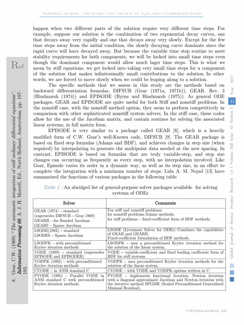
Lida A. M. Nejad
[13]
have
summarized the functions of various packages in the following table
Table 1
:
An abridged list of general-purpose solver packages available
for solving
systems of ODEs
11
Globa
lJo
urna
lof
Scienc
eFr
ontie
rResea
rch
V
olum
eXIII
Issue
e
rsion
IV
VI
Yea
r
2 013
F)
)
© 2013 Global Journals Inc. (US)
Solver Comments
GEAR (1974) – standard (supersedes DIFSUB – Gear 1968) GEARB – for Banded Jacobian GEARS – Sparse Jacobian
For stiff and nonstiff problems;for nonstiff problems-Adams methods, for stiff problems – fixed-coefficient form of BDF methods.
LSODE(1982) – standard LSODES – Sparse Jacobian
LSODE (Livermore Solver for ODEs) Combines the capabilities of GEAR and GEARB.Fixed-coefficient formulation of BDF methods.
LSODPK – with preconditioned Krylov iteration methods
LSODPK – uses a preconditioned Krylov iteration method for the solution of the linear system.
VODE (1989) – standard (supersedes EPISODE and EPISODEB)
VODE – variable-coefficient and fixed leading coefficient form of BDF for stiff systems.
VODPK (1992) – with preconditioned Krylov iteration methods
VODPK – uses preconditioned Krylov iteration methods for the solution of the linear system.
CVODE – in ANSI standard C CVODE – with VODE and VODPK options written in C.PVODE (1995) – Parallel VODE in ANSI standard C with preconditioned Krylov iteration methods.
PVODE – implements functional iteration, Newton iteration with a diagonal approximate Jacobian and Newton iteration with the iterative method SPGMR (Scaled Preconditioned Generalized Minimal Residual).
happen when two different parts of the solution require very different time steps. For
8. G
ear,
C.W
. (1
969)
“ The
auto
mati
c in
tegra
tion o
f st
iff ord
inary
diffe
renti
al eq
uations ”
.
Info
rmati
on P
roce
ssin
g 6
8, A
. J. H
. M
orr
ell, E
d., N
ort
h H
olland, A
mst
erdam
, pp. 187-
193.
Ref
The EPISODE program is a package of FORTRAN subroutines aimed at the
automatic solution of problems, with a minimum effort required in the face of possible
difficulties in the problem. The program implements both a generalized Adams method,
well suited for nonstiff problems, and a generalized backward differentiation formula
(BDF), well suited for stiff problems. Both methods are of implicit multistep type. In
solving stiff problems, the package makes the heavy use of the NN
Jacobian matrix,
N
jij
iJ1,
y
f
y
f
the if and jy
are the vector components of f
and y,
respectively.
A complete discussion of the use of EPISODE is given in [11]. However, a few basic
parameter definitions are needed here, in order to present the examples. Beyond the
specification of the problem itself, represented by example 1 and perhaps example 2, the
most important input parameter to EPISODE is the method flag, MF. This has eight
values-10, 11, 12, 13, 20, 21, 22, and 23. The first digit of MF, called METH, indicates the
two basic methods to be used
namely implicit Adams and BDF.
The second digit, called
MITER, indicates the method of iterative solution of the implicit equations arising from
the chosen formula. The parameter MITER takes four different values (0, 1, 2, 3) to
indicate the following respectively
o
Functional (or fixed-point) iteration (no Jacobian
matrix used.).
o
A
chord method (or generalized Newton method,
or semi-stationary Newton iteration)
with Jacobian given by a subroutine supplied by the user.
o
A
chord
method with Jacobian generated internally by finite differences.
o
A
chord method with a diagonal approximation to the Jacobian, generated internally
(at less cost in storage and computation, but with reduced effectiveness).
The EPISODE package is used by making calls to a driver subroutine, EPSODE,
which in turn calls other routines in the package to solve the problem. The function f
is
communicated by way of a subroutine, DIFFUN, which the user must write. A subroutine
for the Jacobian, PEDERV, must also be written. Calls to EPSODE are made repeatedly,
once for each of the user’s output points. A value of t at which output is desired is put in
the argument TOUT to
EPSODE, and when TOUT is reached, control returns to the
calling program with the value of y at t =TOUT. Another argument to EPSODE, called
INDEX, is used to convey whether or not the call is the first one for the problem (and
thus whether to initialize various variables). It is also used as an output argument, to
convey the success or failure of the package in performing the requested task. Two other
input parameters. EPS and IERROR, determine the nature of the error control performed
within EPISODE.
The
EPISODE package consists of eight FORTRAN subroutines, to be combined
with the user’s calling program and Subroutines DIFFUN and PEDERV. As discussed
earlier, only Subroutine EPSODE is called by the user; the others are called within the
package. The functions of the eight package routines can be briefly summarized as follows:
Ref.
12
Globa
lJo
urna
lof
Scienc
eFr
ontie
rResea
rch
V
olum
eXIII
Issue
e
rsion
IV
VI
Yea
r
2013
F
)
)
© 2013 Global Journals Inc. (US)
11.H
indm
arsh
, A. C
.and B
yrn
e, G. D
. (1975)
“Episo
de. A
n ex
perim
enta
l pack
age fo
r the
integ
ratio
n o
f system
s of o
rdin
ary
differen
tial eq
uatio
ns”, L
.L.L
. Rep
ort U
CID
-30112,
l.l.l.(w
ww
.netlib
.org
/ode/
epso
de.f)
ii)
INTERP computes interpolated values of
y(t) at the user specified output points,
using an array of multistep history data.
iii)
TSTEP performs a single step of the integration, and does the control of local error
(which entails selection of the step size and order) for that step.
iv)
COSET sets coefficients that are used by TSTEP, both for the basic integration step
and for error control.
v)
ADJUST adjusts the history array when the order is reduced.
vi)
PSET sets up the matrix JhIp 0 , where I
is the identity matrix, h
is the step
size, 0
is a scalar related to the method, and J is the Jacobian matrix. It then
processes P for subsequent solution of linear algebraic system with P for subsequent
solution of linear algebraic systems with P as coefficient matrix.
vii)
DEC performs an LU (lower-upper triangular) decomposition of an NN
matrix.
viii)
SOL solves linear algebraic systems for which the matrix was factored by DEC.
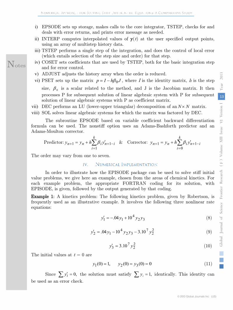
The subroutine EPSODE based on variable coefficient backward differentiation
formula can be used. The nonstiff option uses an Adams-Bashforth predictor and an
Adams-Moulton corrector.
Predictor:
k
iininn yhyy
111
& Corrector:
k
iininn yhyy
011
The order may vary from one to seven.
In order to illustrate how the EPISODE package can be used to solve stiff initial
value problems, we give here an example, chosen from the areas of chemical kinetics. For
each example problem, the appropriate FORTRAN coding for its solution, with
EPISODE, is given, followed by the output generated by that coding.
Example 1:
A kinetics problem:
The following kinetics problem, given by Robertson, is
frequently used as an illustrative example. It involves the following three nonlinear rate
equations:
324
11 1004. yyyy (8)
22
732
412 10.31004. yyyyy (9)
22
73 10.3 yy (10)
The initial values at t
=
0 are
,1)0(1 y 0)0()0( 32 yy (11)
Since ,0iy
the solution must satisfy ,1iy
identically. This identity can
be used as an error check.
13
Globa
lJo
urna
lof
Scienc
eFr
ontie
rResea
rch
V
olum
eXIII
Issue
e
rsion
IV
VI
Yea
r
2 013
F)
)
© 2013 Global Journals Inc. (US)
i) EPSODE sets up storage, makes calls to the core integrator, TSTEP, checks for and
deals with error returns, and prints error message as needed.
Notes
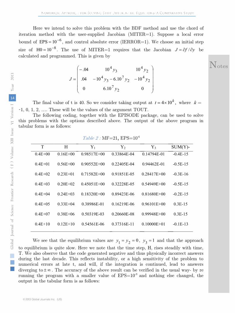
size of
810H0 . The use of MITER=1 requires that the Jacobian yfJ /
be
calculated and programmed. This is given by
010.60
1010.61004.
101004.
27
24
27
34
24
34
y
yyy
yy
J
The final value of t is 40. So we consider taking output at ,104 kt
where k =
-1, 0, 1, 2, …. These will be the values of the argument TOUT.
The following coding, together with the EPISODE package, can be used to solve
this problems with the options described above.
The output of the above program in
tabular form is as follows:
Table 2
:
MF=21, EPS=10-6
T
H
Y1
Y2
Y3
SUM(Y)-
1
0.4E+00
0.16E+00
0.98517E+00
0.33864E-04
0.14794E-01
-0.4E-15
0.4E+01
0.56E+00
0.90552E+00
0.22405E-04
0.94462E-01
-0.5E-15
0.4E+02
0.23E+01
0.71582E+00
0.91851E-05
0.28417E+00
-0.3E-16
0.4E+03
0.20E+02
0.45051E+00
0.32228E-05
0.54949E+00
-0.5E-15
0.4E+04
0.24E+03
0.18320E+00
0.89423E-06
0.81680E+00
-0.2E-15
0.4E+05
0.33E+04
0.38986E-01
0.16219E-06
0.96101E+00
0.3E-15
0.4E+07
0.38E+06
0.50319E-03
0.20660E-08
0.99948E+00
0.3E-15
0.4E+10
0.12E+10
0.54561E-06
0.37316E-11
0.10000E+01
-0.1E-13
We see that the equilibrium values are
021 yy , 13 y
and that the approach
to equilibrium is quite slow. Here we note that the time step, H, rises steadily with time,
T. We also observe that the code generated negative and thus physically incorrect answers
during the last decade. This reflects instability, or a high sensitivity of the problem to
numerical errors at late t, and will, if the integration is continued, lead to answers
diverging to .
The accuracy of the above result can be verified in the usual way-
by re
running the program with a smaller value of EPS=10-9 and nothing else changed, the
output in the tabular form is as follows:
14
Globa
lJo
urna
lof
Scienc
eFr
ontie
rResea
rch
V
olum
eXIII
Issue
e
rsion
IV
VI
Yea
r
2013
F
)
)
© 2013 Global Journals Inc. (US)
Here we intend to solve this problem with the BDF method and use the chord of
iteration method with the user-supplied Jacobian (MITER=1). Suppose a local error
bound of 610EPS , and control absolute error (IERROR=1). We choose an initial step
Notes
0.4E+01
0.14E+00
0.905519E+00
0.224048E-04
0.944589E-01
0.5E-15
0.4E+02
0.13E+01
0.715827E+00
0.918552E-05
0.284164E+00
0.6E-15
0.4E+03
0.82E+01
0.450519E+00
0.322290E-05
0.549478E+00
0.8E-15
0.4E+04
0.76E+02
0.183202E+00
0.894237E-06
0.816797E+00
0.1E-14
0.4E+05
0.88E+03
0.389834E-01
0.162177E-06
0.961016E+00
0.9E-15
0.4E+07
0.20E+06
0.516813E-03
0.206835E-08
0.999483E+00
0.1E-14
0.4E+10
0.67E+09
0.522363E-06
0.208942E-11
0.999999E+00
0.1E-14
100
102
104
106
108
T
10-10
10-8
10-6
10-4
10-2
100
Y1,Y2,Y3
Y2
Y1
Y3
100
102
104
106
108
1010
T
10-11
10-9
10-7
10-5
10-3
10-1
Y1,Y2,Y3
Y1
Y2
Y3
EPS=10-6
EPS=10-9
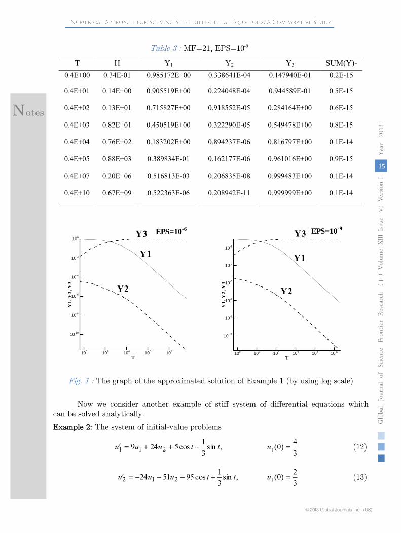
Fig. 1
:
The graph of the approximated solution of Example 1 (by using log scale)
Now we consider another example of stiff system of differential equations which
can be solved analytically.
Example
2: The
system of initial-value problems
,sin31cos5249 211 ttuuu
34)0(1 u (12)
,sin31cos955124 212 ttuuu
32)0(1 u (13)
15
Globa
lJo
urna
lof
Scienc
eFr
ontie
rResea
rch
V
olum
eXIII
Issue
e
rsion
IV
VI
Yea
r
2 013
F)
)
© 2013 Global Journals Inc. (US)
Table 3 : MF=21, EPS=10-9
T H Y1 Y2 Y3 SUM(Y)-
10.4E+00 0.34E-01 0.985172E+00 0.338641E-04 0.147940E-01 0.2E-15
Notes
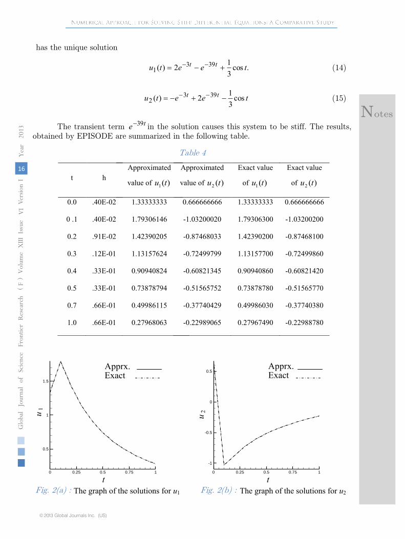
The transient term te 39 in the solution causes this system to be stiff.
The results,
obtained by EPISODE are summarized in the following table.
Table 4
t
h
Approximated
value of )(1 tu
Approximated
value of )(2 tu
Exact value
of )(1 tu
Exact value
of )(2 tu
0.0
.40E-02
1.33333333
0.666666666
1.33333333
0.666666666
0 .1
.40E-02
1.79306146
-1.03200020
1.79306300
-1.03200200
0.2
.91E-02
1.42390205
-0.87468033
1.42390200
-0.87468100
0.3
.12E-01
1.13157624
-0.72499799
1.13157700
-0.72499860
0.4
.33E-01
0.90940824
-0.60821345
0.90940860
-0.60821420
0.5
.33E-01
0.73878794
-0.51565752
0.73878780
-0.51565770
0.7
.66E-01
0.49986115
-0.37740429
0.49986030
-0.37740380
1.0
.66E-01
0.27968063
-0.22989065
0.27967490
-0.22988780
0 0.25 0.5 0.75 1T
0.5
1
1.5
U1
Apprx.Exact
0 0.25 0.5 0.75 1T
-1
-0.5
0
0.5
U2
Apprx.Exact
The graph of the solutions for u1
The graph of the solutions for u2
u
1
u
2
t
t
16
Globa
lJo
urna
lof
Scienc
eFr
ontie
rResea
rch
V
olum
eXIII
Issue
e
rsion
IV
VI
Yea
r
2013
F
)
)
© 2013 Global Journals Inc. (US)
has the unique solution
.cos312)( 393
1 teetu tt (14)
teetu tt cos312)( 393
2 (15)
Fig. 2(a) : Fig. 2(b) :
Notes
effective codes available to solve these problems, but it is necessary that the user may
have some idea how they work in order to take full advantage of them. Although a
number of methods have been developed, and many more basic formulas are suggested for
stiff equations, until now there has been little advice or guidance to help a user choose a
good method for his problem. In our study we focus on a particularly efficient program
which is named as EPISODE. We explain the capabilities of this code and present few
practical examples for which it is effective. However, this experimental package EPISODE
requires some explanation. First of all, the program is relatively new and has not been
used extensively, and so its position in the field of existing available ordinary differential
equation software is not yet clear. Secondly we have shown that, for some types of
problems, the program spends more time on the linear system of the algorithm than we
feel it should. This behavior is related to the extent to which the matrix during the
solution of a problem, and in this area improvement of the efficiency of the algorithm is
required.
1.
Lapidus, L.
and Schiesser, W.E. (1976), Numerical Methods For Differential System. Academic press, INC. (London).
2.
Shampine, L. F.
and Gear, C.W.
(Jan, 1979) “A user’s View of Solving Stiff Ordinary
Differential Equations”,
SIAM Review,
Vol.21, No.1, pp 1-17
3.
Byrne, George D and Hindmarsh, A.C. (March 1986) “Stiff ODE Solvers: A review of
current and coming attractions”. Journal of Computational Physics, Vol.70, Issue 1,
pp 1-62.
4.
Burden, R. L., Faires, J. D. (2002); Numerical Analysis, 7 th
edition, PWS Publishers,
U.S.A.
5.
Atkinson, Kendall E. (1989) An introduction to Numerical Analysis.
John Wiley &
Sons.
6.
Gerald, F. Curtis and Wheatley O. Patrick (1999), Applied Numerical Analysis,
6 th
edition. Pearson Education, Inc.
7.
Enright, W.H. and HULL, T.E.
(1976) “Comparing Numerical Methods for the
solution of Stiff Systems of ODEs Arising in Chemistry”,
Numerical Method,
Academic Press Orlando, pp 45-57.
8.
Gear, C.W. (1969) “The automatic integration of stiff ordinary differential equations”.
Information Processing 68, A. J. H. Morrell, Ed., North Holland, Amsterdam, pp. 187-
193.
17
Globa
lJo
urna
lof
Scienc
eFr
ontie
rResea
rch
V
olum
eXIII
Issue
e
rsion
IV
VI
Yea
r
2 013
F)
)
Notes
© 2013 Global Journals Inc. (US)
Here we observe that the graph of the approximated solution and the graph of the
exact solution coincide with each other.
In this paper our aim is to study the phenomenon of stiff differential equations and
the general purpose procedures for the solution of stiff differential equations. There are
9. Gear, C.W. (1971), “Algorithm 407: DIFSUB for solution of ordinary differential
equations”, Comm. ACM, Vol.14, No. 3, pp.185-190
13.
Nejad, Lida A.M.
(2005) “A comparison of stiff ODE solvers for astrochemical kinetics
problems”, Astrophysics and Space Science. Vol. 299, pp. 1-29.
18
Globa
lJo
urna
lof
Scienc
eFr
ontie
rResea
rch
V
olum
eXIII
Issue
e
rsion
IV
VI
Yea
r
2013
F
)
)
© 2013 Global Journals Inc. (US)
11. Hindmarsh, A. C. and Byrne, G. D. (1975) “Episode. An experimental package for the
integration of systems of ordinary differential equations”, L.L.L. Report UCID-30112, l.l.l. (www.netlib.org/ode/epsode.f)
12. Hindmarsh, A. C. and Gear C.W. (1974), “Ordinary differential equation system
solver”, L.L.L. Report UCID -30001, rev. 3, l.l.l. (www.netlib.org/ode/epsode.f)
10. Byrne, G. D. and Hindmarsh, A. C. (1975) “A polyalgorithm for the numerical
solution of ordinary differential equations”, ACM Transactions on Mathematical Software, Vol.1, pp. 71-96
Notes
Related Documents