Hindawi Publishing Corporation Journal of Fluids Volume 2013, Article ID 532016, 11 pages http://dx.doi.org/10.1155/2013/532016 Research Article Numerical and Experimental Analysis of the Growth of Gravitational Interfacial Instability Generated by Two Viscous Fluids of Different Densities Snehamoy Majumder, Debajit Saha, and Partha Mishra Department of Mechanical Engineering, Jadavpur University, Kolkata 700 032, West Bengal, India Correspondence should be addressed to Debajit Saha; [email protected] Received 30 April 2013; Revised 20 August 2013; Accepted 4 September 2013 Academic Editor: Andrew W. Cook Copyright © 2013 Snehamoy Majumder et al. is is an open access article distributed under the Creative Commons Attribution License, which permits unrestricted use, distribution, and reproduction in any medium, provided the original work is properly cited. In the geophysical context, there are a wide variety of mechanisms which may lead to the formation of unstable density stratification, leading in turn to the development of the Rayleigh-Taylor instability and, more generally, interfacial gravity-driven instabilities, which involves moving boundaries and interfaces. e purpose of this work is to study the level set method and to apply the process to study the Rayleigh-Taylor instability experimentally and numerically. With the help of a simple, inexpensive experimental arrangement, the R-T instability has been visualized with moderate accuracy for real fluids. e same physical phenomenon has been investigated numerically to track the interface of two fluids of different densities to observe the gravitational instability with the application of level set method coupled with volume of fraction replacing the Heaviside function. Good agreement between theory and experimental results was found and growth of instability for both of the methods has been plotted. 1. Introduction e Rayleigh-Taylor instability is instability of an interface of two fluids of different densities which occurs when the interface between the two fluids is subjected to a normal pressure gradient with direction such that the pressure is higher in the light fluid than in the dense fluid. is is the case with an interstellar cloud and shock system. A similar situation occurs when gravity is acting on two fluids of different density—with the denser fluid above a fluid of lesser density—such as water balancing on light oil. Considering two completely plane-parallel layers of immiscible fluid, the heavier on top of the light one and both subject to the Earth’s gravity, the equilibrium here is unstable to certain perturbations or disturbances. An unstable disturbance will grow and direct to a release of potential energy, as the heavier material moves down under the gravitational field and the lighter material is displaced upwards. Such instability can be observed in many situations including technological applications as laser implosion of deuterium-tritium fusion targets, electromagnetic implosion of a metal liner and natural phenomena as overturn of the outer portion of the collapsed core of a massive star, and the formation of high luminosity twin-exhaust jets in rotating gas clouds in an external gravitational potential. Various numerical and experimental works have been done by many researchers concentrating on the growth of single wavelength perturbations as well as considering different wavelength modes. Sharp [1] presented some of the critical issues concerning Rayleigh-Taylor instability. e importance to carry out the three-dimensional study of Tay- lor instability and the role of statistically distributed hetero- geneities on the growth of instability have been analyzed in his work. Read [2] experimentally investigated the turbulent mixing by Rayleigh-Taylor instability and the results showed that if the instability arises from small random perturbations, the width of the mixed region grows in proportion to 2 . e same investigation has been done numerically by Youngs [3] to simulate the growth of perturbations at an interface between two fluids of different density. If the mixing process evolves from small perturbations then the growth of instabil- ity is controlled by the non-linear interaction between bub- bles of different sizes. Dalziel [4] investigated the Rayleigh- Taylor instability experimentally using a simple apparatus

Welcome message from author
This document is posted to help you gain knowledge. Please leave a comment to let me know what you think about it! Share it to your friends and learn new things together.
Transcript
Hindawi Publishing CorporationJournal of FluidsVolume 2013 Article ID 532016 11 pageshttpdxdoiorg1011552013532016
Research ArticleNumerical and Experimental Analysis of the Growth ofGravitational Interfacial Instability Generated by Two ViscousFluids of Different Densities
Snehamoy Majumder Debajit Saha and Partha Mishra
Department of Mechanical Engineering Jadavpur University Kolkata 700 032 West Bengal India
Correspondence should be addressed to Debajit Saha debajitsaha1986gmailcom
Received 30 April 2013 Revised 20 August 2013 Accepted 4 September 2013
Academic Editor AndrewW Cook
Copyright copy 2013 Snehamoy Majumder et al This is an open access article distributed under the Creative Commons AttributionLicense which permits unrestricted use distribution and reproduction in any medium provided the original work is properlycited
In the geophysical context there are awide variety ofmechanismswhichmay lead to the formation of unstable density stratificationleading in turn to the development of the Rayleigh-Taylor instability and more generally interfacial gravity-driven instabilitieswhich involves moving boundaries and interfaces The purpose of this work is to study the level set method and to apply theprocess to study the Rayleigh-Taylor instability experimentally and numericallyWith the help of a simple inexpensive experimentalarrangement the R-T instability has been visualized with moderate accuracy for real fluids The same physical phenomenon hasbeen investigated numerically to track the interface of two fluids of different densities to observe the gravitational instability withthe application of level set method coupled with volume of fraction replacing the Heaviside function Good agreement betweentheory and experimental results was found and growth of instability for both of the methods has been plotted
1 Introduction
The Rayleigh-Taylor instability is instability of an interfaceof two fluids of different densities which occurs when theinterface between the two fluids is subjected to a normalpressure gradient with direction such that the pressure ishigher in the light fluid than in the dense fluid This is thecase with an interstellar cloud and shock system A similarsituation occurs when gravity is acting on two fluids ofdifferent densitymdashwith the denser fluid above a fluid of lesserdensitymdashsuch as water balancing on light oil Consideringtwo completely plane-parallel layers of immiscible fluid theheavier on top of the light one and both subject to theEarthrsquos gravity the equilibrium here is unstable to certainperturbations or disturbances An unstable disturbance willgrow and direct to a release of potential energy as theheavier material moves down under the gravitational fieldand the lighter material is displaced upwards Such instabilitycan be observed in many situations including technologicalapplications as laser implosion of deuterium-tritium fusiontargets electromagnetic implosion of a metal liner andnatural phenomena as overturn of the outer portion of
the collapsed core of a massive star and the formation ofhigh luminosity twin-exhaust jets in rotating gas clouds in anexternal gravitational potential
Various numerical and experimental works have beendone by many researchers concentrating on the growthof single wavelength perturbations as well as consideringdifferent wavelength modes Sharp [1] presented some ofthe critical issues concerning Rayleigh-Taylor instability Theimportance to carry out the three-dimensional study of Tay-lor instability and the role of statistically distributed hetero-geneities on the growth of instability have been analyzed inhis work Read [2] experimentally investigated the turbulentmixing by Rayleigh-Taylor instability and the results showedthat if the instability arises from small random perturbationsthe width of the mixed region grows in proportion to 119905
2The same investigation has been done numerically by Youngs[3] to simulate the growth of perturbations at an interfacebetween two fluids of different density If the mixing processevolves from small perturbations then the growth of instabil-ity is controlled by the non-linear interaction between bub-bles of different sizes Dalziel [4] investigated the Rayleigh-Taylor instability experimentally using a simple apparatus
2 Journal of Fluids
of novel design where the initial nonlinear perturbations tothe flow have been introduced by the removal of the barrierseparating the two fluid layers and a good agreement betweenthe results of this work and a previous one has been achievedVelocity measurements have been done by particle trackingusing the method of particle image velocimetry Voropayevet al [5] experimentally analyzed the evolution of gravita-tional instability of an overturned initially stable stratifiedfluid In the present analysis the instability is initiated byoverturning the experimental setup such that the heavyfluid lies over the lighter one The present study is mainlyconcerned about the propagating interface between the twofluids and its formation and growth rate A propagatinginterface is a closed surface in some space that is movingunder a function of local global and independent prop-erties A variety of numerical algorithms are available totrack propagating interfaces and in the present numericalsimulation level set method coupled with volume of fractionhas been used Level set method is a computational techniquefor tracking moving interfaces which rely on an implicitrepresentation of the interface whose equation of motion isnumerically approximated using schemes built from those forhyperbolic-conservation laws The consequential techniquesare able to handle problems inwhich the speed of the evolvinginterface may sensitively depend on local properties such ascurvature and normal direction as well as complex physicsof the front and internal jump and boundary conditionsdetermined by the interface location
The volume of fluid (VOF) technique has been presentedby Hirt and Nichols [6] as a simple and efficient means fornumerically handling free boundaries in a calculation meshof Eulerian or arbitrary Lagrangian-Eulerian cells It worksextremely well for a wide range of complicated problems andthis process is very much conservative in nature but theappropriate tracking of the interface is not possible by thismethod
Sethian [7] presented a case of the evolution of a frontpropagating along its normal vector field with curvature-dependent speed Numerical methods based on finite dif-ference schemes for marker particles along the front areshown to be unstable in regions where the curvature buildsrapidly And then the front tracking based on volume offluid techniques has been used together with the entropycondition
Various numerical methods were developed to studythe propagating interfaces Osher and Sethian [8] devisednew numerical algorithms called PSC algorithms for frontspropagating with curvature-dependent speed Merrimanet al [9] extended the Hamilton Jacobi formulation of Osherand Sethian and proposed a level set method for the motionofmultiple junctionswhere the diffusion equationwas shownto generate curvature-dependent motion Zhu and Sethian[10] considered hydrodynamic problems with cold flamepropagation by merging a second-order projection methodfor viscous Navier stokes equations with modern techniquesfor computing the motion of interfaces propagating withcurvature-dependent speed A newmethod was presented byUnverdi and Tryggvasan [11] to simulate unsteady multifluid
flows in which a sharp interface or a front separates incom-pressible fluids of different density and viscosity Chopp andSethian [12] studied hyper surfaces moving under flow thatdepends on the mean curvature The approach was based ona numerical technique that embeds the evolving hypersurfaceas the zero Level Set of a family of evolving surfaces Sussmanet al [13] combined a level set method with a variable densityprojection method for capturing the interface between twofluids to allow for computation of two-phase flow where theinterface can merge or break considering a high Reynoldsnumber Chang et al [14] presented a level set formulationfor incompressible immiscible multi fluid flow separated bya free surface and the interface was identified as the zero LevelSet of a smooth function
Theory and algorithms of level set method were reviewedby Sethian [15] for the evaluation of the complex inter-faces Topological changes corner and cusp developmentand accurate determination of geometric properties such ascurvature andnormal directionwere obtained by themethodFew years later Sethian [16] summarized the developmentand interconnection between narrow band level set methodand fast marching method which provides efficient tech-niques for tracking moving fronts At another paper Sethian[17] reviewed past works on fast marching method and levelsetmethod for tracking propagating interfaces in two or threespace dimensions
Kaliakatos and Tsangaris [18] studied the motion ofdeformable drops in pipes and channels using a level setapproach in order to capture the interface of two fluidsThe shape of the drop the velocity field and the additionalpressure loss due to the presence of the drop the relativesize of the drop to the size of the pipe or channel cross-section the ratio of the drop viscosity to the viscosity ofthe suspending fluid and the relative magnitude of viscousforces to the surface tension forces were computed Son andHur [19] combined a level set method with the volume offluid method to calculate an interfacial curvature accuratelyas well as to achieve mass conservation They developeda complete and efficient interface reconstruction algorithmwhich was based on the explicit relationship between theinterface configuration and the fluid volume function
Sethian and Smereka [20] provided an overview oflevel set methods introduced by Osher and Sethian [8]for computing the solution to fluid-interface problemsThey discussed the essential ideas behind the computa-tional techniques that rely on an implicit formulation ofthe interface and the coupling of these techniques to finite-differencemethods for incompressible and compressible flowMajumder andChakraborty [21] developed a novel physicallybased mass conservation model in the skeleton of a levelset method as a substitute to the Heaviside function basedformulation The transient evolution of a rounded bubble ina developing shear flow and rising bubbles in a static fluid theCox angle and the deformation parameter characterizing thebubble evolution were critically examined Carles et al [22]used a magnetic field gradient to draw down a low densityparamagnetic fluid below a more dense fluid in a Hele-Shawcell An extended level set method for classical shape andtopology optimization was proposed based on the popular
Journal of Fluids 3
radial basis functions byWang et al [23]The implicit level setfunction was approximated by using the RBF implicit mod-eling with multiquadric splines Sun and Tao [24] presenteda coupled volume of fluid and level set (VOSET) methodfor computing incompressible two-phase flows VOFmethodwas used to conserve the mass and level set method wasused to get the accuracy of curvature and smoothness ofdiscontinuous physical quantities near interfaces Sussmanand Puckett [25] presented a coupled level setvolume-of-fluid (CLSVOF)method for computing 3D and axisymmetricincompressible two-phase flows and Sussman [26] presenteda coupled level set and volume of fluidmethod for computinggrowth and collapse of vapor bubbles A level set methodwas combined with the volume of fluid method by Son[27] for computing incompressible two-phase flows in threedimensions where the interface configurations were muchmore diverse and complicated A passive scalar transportmodel has been studied by Wang et al [28] to study the 3DRayleigh-Taylor instability The characteristic behavior andthe principle of the interfacial motion from both sinusoidaland random perturbations have been achieved Youngs [29]numerically simulated three-dimensional turbulent mixingof miscible fluids of RT instability which concluded thatsignificant dissipation of turbulent fluctuations and kineticenergy occurs via the cascade to high wave numbers Thechaotic stage of Rayleigh-Taylor instability is characterized bythe evolution of bubbles of the light fluid and spikes of theheavy fluid Gardner et al [30] proposed a statistical modelto analyze the growth of bubbles in aRayleigh-Taylor unstableinterface The model using numerical solutions based on thefront tracking method has been compared to the solutionsof the full Euler equations for compressible two-phase flowLater Glimm et al [31] numerically studied the dynamicsof the bubbles in chaotic environment and their interactionswith each other as well as the acceleration of the bubbleenvelope
The Rayleigh-Taylor instability is a gravity driven insta-bility of a contact surface and this growth of this instabilityis sensitive to numerical or physical mass diffusion Li et al[32] addressed this problem using a second-order TVD finitedifference scheme with artificial compression They numeri-cally simulated the 3D Rayleigh-Taylor instability using thisscheme A new model was proposed by Chen et al [33 34]for the momentum coupling between the two phases TheRayleigh-Taylor instability of an interface separating fluids ofdistinct density is driven by acceleration across the interfaceTwo-phase turbulent mixing data were analyzed which havebeen obtained from direct numerical simulation of the two-fluid Euler equations by the front tracking method Directnumerical simulation of three-dimensional Rayleigh-Taylorinstability (RTI) between two incompressible miscible fluidshas been presented by Cook and Dimotakis [35] Mixingwas found to be even more sensitive to initial conditionsthan growth rates The flow structure and energy budgetfor Rayleigh-Taylor instability using the results of a highresolution direct numerical simulation have been examinedby Cook and Zhou [36] Later Cook et al [37] described largeeddy simulation for computing RT instability A relation hasbeen obtained between the rate of growth of the mixing layer
1205882
1205881
x
y = b
y = minusb
y = 0 b
b
y
w
Figure 1 Geometrical presentation of analysis of Rayleigh-Taylorinstability of a dense fluid overlying a lighter fluid
and the net mass flux through the plane associated with theinitial location of the interface
In this present work the level set methodology has beenapplied to visualize theoretically the RT instability using atriangular distribution of initial disturbance The fraction ofvolume in the interface control volumes has been successfullyincorporated for identifying the interface very accuratelyThetopological changes with time have been captured accuratelyand this has been matched effectively with the experimentalresults The instability growth rate which is predicted bythe theory is confirmed by the experimentation with theinitial incipience of linear distribution of disturbances asalready stated This is a positive contribution along with thetheoretical topological visualization of the RT effects
On the other hand themerging and consequent breakingup of the interfaces has been captured while the RT instabilitygrowth takes place These results are important as theyprovides the probable trapping merging and consequentbreaking of the oil and natural gas pools trapped betweenthe formation of salt domes and overlying sedimentaryrocks These effects of the geothermal RT instabilities anddeformation of the rocks above the salt domes are importantas they provide the possibility of exploration of oil and gaspools thus coagulated and subsequent fragmented in hugemass under the earth for million of years These results areencouraging and can bridge our knowledge of RT to apply tothe oil and gas industry
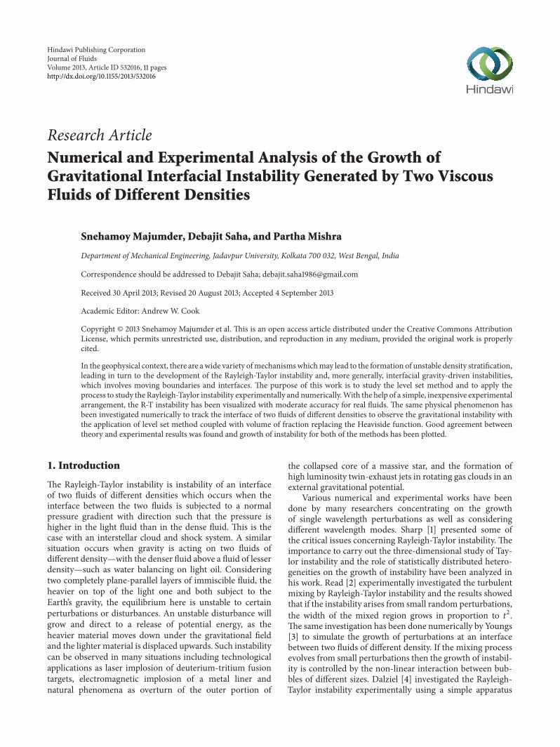
2 Geometrical Description
The geometry of the problem is shown in Figure 1 A fluidlayer with a thickness 119887 and density 120588
1overlies a second layer
of thickness 119887 and density 1205882 The upper boundary and lower
boundary are assumed to be rigid surfaces Here 1205881is greater
than 1205882 The undisturbed interface between fluid layers is
taken to be at 119910 = 0 Due to gravitational instability theinterface between the fluids distorts and motions occurs inthe fluid layersThe displacement of the disturbed fluid layersis denoted by 119908 When the heavy fluid lies above the lightfluid the configuration becomes unstable The time to growthe instability depends on the viscosity of the fluid and thedensity difference of the fluidsWhen the viscosity of the fluidis high and the density difference is smaller the instabilitytakes longer to grow
4 Journal of Fluids
Handle Handle
15 cm
Holes for pouringliquid
1205881 gt 1205882
102 cm204 cm
1205881
1205882
Figure 2 Diagram of the experimental setup
3 Experimental Setup
The experimental setup consists of a closed rectangular boxmade of Perspex of 204 cm times 102 cm times 15 cm dimensionThere are two openings at the top surface with valve arrange-ment for the purpose of filling the box with the requiredliquids The two side handles are provided for convenienceturning of the setup to upside down or vice versa in quicktime The setup is placed on a preleveled surface and lowerhalf of the box is filled with glucose solution and upper halfis filled with colored refined soya bean oil with the help offunnels The viscosities of both the liquids were measuredin the laboratory at room temperature by ldquoFalling Spheremethodrdquo and density of the fluids was measured by simplymeasuring their mass and volume (see Figure 2)
The viscosity and specific gravity of the liquids have beenmeasured as follows
Viscosity of glucose syrup = 350 Pa-SViscosity of oil = 00791 Pa-SSpecific Gravity of Glucose syrup = 14Specific Gravity of oil = 092
4 Experimental Technique
In the experiment first the setup rests at position 3 wherethe light fluid lies over the heavy one In this position it istotally balanced and stable Then the setup is turned upsidedown quickly so that heavy liquid lies in the upper half andthus instability is initiatedThe instability can also be initiatedby keeping the setup at position 2 where the heavy and lightliquids stand vertically side by side in an unbalanced andunstable condition Naturally all these configurations wantto return to position 3 to minimize the potential energy andto gain a stable and balanced position The whole processis captured to track the moving interface and to study thegrowth rate of the instability with time (see Figure 3)
5 Formulation of Two-Phase Flow withSurface Tension
The term two-phase flow refers to the motion of two differentinteracting fluids or with fluids that are in different phasesIn the present analysis only two immiscible incompressiblefluids have been considered and a low enough Reynolds
number is assumed so that the flow can be considered aslaminar flow Level set method may be applied to track theinterface efficiently in case of incompressible immisciblefluids in which steep gradient in viscosity and density existedacross the interface In these problems the role of surfacetension is crucial and formed an important part of thealgorithm
6 Numerical Modeling
For mathematical analysis we assume a system of two-fluid phases constituting a two-dimensional domain Theindividual fluid phases are assumed to be incompressible butdeformable in shape on account of shear stresses prevailingbetween various fluid layers as well as fluid-solid interfacesWe assume the flow field to be two dimensional and laminar
Navier-Stokes equation is given as
119906119905+ (119906 sdot nabla) 119906 = 119865 +
1
120588(minusnabla119875 + 120583nabla
2119906 + ST) (1)
Assume a sharp fluid interface between two fluids withdifferent densities and also the flow is incompressible andthus
nabla sdot 119906 = 0 (2)
The surface tension term acts normal to the fluid interfaceand is proportional to the curvature due to balance of forceargument between the pressure on each side of the interfaceThis leads to the relation
ST = 120590120581120575 (119889) 119899 (3)
Thus surface tension acts as an additionally forcing term inthe direction normal to the fluid interface
Now replacing normal 119899 by nabla120601|nabla120601| and when distance 119889is approximated by nabla120601|nabla120601| we have
120590120581120575 (119889) 119899 = 120590120581 (120601) 120575 (120601) nabla120601 (4)
The curvature 119896(120601) can be expressed by 120601 and its derivativesas follows
119896 (120601) = minus
1206012
119910120601119909119909
minus 2120601119909120601119910120601119909119910
+ 1206012
119909120601119910119910
(1206012
119909+ 1206012
119910)32
(5)
As in [14] regularized delta function 120575(120601) can be defined as
120575 (120601) equiv
12 (1 + cos (120587119909120576))120576
if |119909| lt 120576
0 Otherwise(6)
This recasts the surface tension in the level set framework If 120601is always reinitialized to the distance function the Dirac deltafunction itself can be smoothed
Thus the equation of motion become
119906119905+ (119906 sdot nabla) 119906 = 119865 +
1
120588(minusnabla119875 + 120583nabla
2119906 + 120590120581 (120601) 120575 (120601) nabla120601)
nabla sdot 119906 = 0
(7)
The governing equations can be written as follows
Journal of Fluids 5
Small perturbation
Heavy liquid
Light liquid
Unstable but balanced
Unstable and unbalanced
Stable and balanced
Position 1
Position 2
Light liquid
Heavy liquid
Heavyliquid
Lightliquid
Position 3
Figure 3 Illustration of different types of stability and experimental procedure
61 Continuity Consider
120597120588
120597119905+
120597 (120588119906119895)
120597119909119895
= 0 (8)
62 Momentum Consider
120588120597119906119894
120597119905+ 120588119906119895
120588119906119894
120597119909119895
=120597
120597119909119895
(120583120597119906119894
120597119909119895
) minus120597119901
120597119909119894
+ 120588119892119894
+ 120590120581 (120601) nabla120601120575 (120601)
(119894 119895 = 1 2)
(9)
A scalar variable level set function is used to identifythe interface between two fluids and also acts as a distancefunction The equation transporting the interface can bewritten as
120597120601
120597119905+ 119906119895
120597120601
120597119909119895
= 0 (10)
where 120601(119909119895119905) is the level set function prescribing position of
the interface at any specified time instant If the value of the120601 at the interface is taken as zero it effectively becomes adistance function satisfying
1003816100381610038161003816nabla120601
1003816100381610038161003816= 1 (11)
But at all instant of times 120601 must remain a distancefunction to ensure that another scalar variable needs to beintroduced and solvedThis variable (120595)must be constrainedto constitute a distance function having the same interfacevalue as 120601 This can be achieved by obtaining a pseudo-steady-state solution for the following transient transportequation of 120595
120597120595
120597119905
= sign (120595) (1 minus 1003816100381610038161003816nabla120595
1003816100381610038161003816) (12)
where1003816100381610038161003816nabla120595
1003816100381610038161003816= radic(120595
2
119909+ 1205952
119910) (13)
with 119905 being a pseudo-time stepEquation (12) is subjected to the following initial
condition120595 (119883 0) = 120601 (119883 119905 + Δ119905) (14)
The reinitialization process is iteration of (12) with apseudo-time step and within a few iterations it comes to asteady state solutionThen the reinitialization procedure endsleading to reassignment of the level set value
It is evident that pseudo-steady-state value of 120595 is thevalue of 120601 at the time instant (119905 + Δ119905) Success of the masscorrection is affected by (12) which depends on the accuracyof the interpolation of physical properties such as densityand viscosity across the interface This can be achieved bycalculating a property 120585 within a control volume as
120585 = [1 minus 119867 (120601)] 1205851+ 119867 (120601) 120585
2 (15)
where119867(120601) is called Heaviside functionThe equation for the one-dimensional volume fraction is
given by
119867 = 05 + (120601
Δ119883) (16)
and for two-dimensional volume fraction the concept hasbeen taken from [21]
At the solid boundary the Neumann boundary conditionfor the level set function has been utilized
7 Solution Procedure
The governing differential equations coupled with appropri-ate boundary conditions are solved using a pressure basedfinite volume method as per the SIMPLER algorithm [38]
6 Journal of Fluids
N
W
S
sJs
Jw
Δx
Δye
Je
nJn
E
P
w
(a)
EP
e
(b)
Figure 4 (a) Control volume for the two-dimensional situation (b) Control volume of 119906
Z
Y
g
O
Light fluid
Heavy fluid Light fluid
Heavy fluid
X
Figure 5 Illustration of the experimental technique
Convection-diffusion terms in the conservation equations arediscretized using the power law scheme [38]
The location of the interface at time 119905 = 0 has beenspecified and then the normal distance for all nodes fromthe interface is calculated The properties at all nodes havebeen specified using (15) The continuity and momentumconservation equations at time instant (119905 + Δ119905) are solvedThen using the velocities obtained in a previous step using(10) 120601 has been solved Next using the values of 120601 frompreceding step as initial values the pseudo-steady-state 120601 (12)has been solved Setting 120601(119909 119905 + Δ119905) = 120595(119909) the procedure isgoing on until the desired convergence is achieved
The temporal term of the momentum equation has beendiscretized as follows Equation (9) in two-dimensional formis discretized to get algebraic linear simultaneous equationsas follows
120597
120597119905(120588120601) +
120597119869119909
120597119909+
120597119869119910
120597119910= 119878 (17)
where 120601 represents general variables and 119869119909and 119869119910are the
total (convection plus diffusion) fluxes defined by
119869119909= 120588119906120601 minus Γ
120597120601
120597119909 119869
119910= 120588V120601 minus Γ
120597120601
120597119910 (18)
where 119906 and V denote the velocity components in the 119909 and 119910directions 119878 is the source term and Γ represents the diffusioncoefficient The integration of (17) over the control volume(Figure 4(a)) gives
(120588119875120601119875minus 1205880
1198751206010
119875) Δ119909Δ119910
Δ119905+ 119869119890minus 119869119908+ 119869119899minus 119869119904
= (119878119862+ 119878119875120601119875) Δ119909Δ119910
(19)
0
05
1
15
2
25
3
35
0 5 10 15 20
Expe
rimen
tal g
row
th w
(cm
)
Time t (s)
Experimental growth rateExpon (experimental growth rate)
w = 0468 e0110t
Figure 6 Development of growth of instability
The source term is linearized in the usual manner antici-pating negative slope while the unsteady terms 120588
119875and 120601
119875are
assumed to prevail over thewhole control volume In a similarfashion the continuity equation is also linearized
Similarly the pressure gradient term is discretized consid-ering the staggered control volume as
119906119890=sum119886119899119887119906119899119887+ 119887
119886119890
+ (119875119875minus 119875119864) 119889119890 (20)
where 119889119890= 119860119890119886119890
This is for the 119906 equation as shown in Figure 4(b) Thecorresponding other equations are discretized in a similarfashion Finally guessing the velocity field the pressure equa-tion is solved and consequently by correcting the velocityfield the variables are solved This method has an essencephysically possible solution by removing unrealistic checkerboard results
8 Results and Discussions
81 Gravitational Instability due to Density Difference withInitially Horizontal Layers of Fluids If the box is rotatedin the YZ plane quickly so that the heavy liquid occupiesthe upper portion then instability will initiate at once in
Journal of Fluids 7
0
05
1
15
2
25
3
35
4
0 5 10 15 20Time t (s)
Gro
wth
w(c
m)
Figure 7 Development of growth of instability as found by theo-retical modeling
0
05
1
15
2
25
3
35
4
45
0 5 10 15 20Time t (s)
ExperimentalTheoretical
Gro
wth
w(c
m)
Figure 8 Comparison of the development of the growth ofinstability
the presence of sufficient unavoidable perturbations and theinterface starts movingThe position of the interface at differ-ent times especially in the initial stage of growing instabilityhas been analyzed in the present investigation (see Figure 5)
82Theoretical Growth of Instability From theoretical analy-sis of the problem the growth rate is given by
120597119908
120597119905=
(1205881minus 1205882) 119892119887
4120583
times (((120582
2120587119887)
2
tanh 2120587119887
120582
minus1
sinh (2120587119887120582) cosh (2120587119887120582))
times(120582
2120587119887+
1
sinh (2120587119887120582) cosh (2120587119887120582))
minus1
) times 119908
(21)
0
01
02
03
04
05
06
0 1 2 3 4 5
Theoretical growth rateGrowth w (cm)
Experimental growth rate
Gro
wth
rate
120575w
120575t
(cm
s)
Figure 9 Comparison of the growth Rate of the instability
Figure 10 Distribution of initial instability triggered for the numer-ical analysis
Here it has been assumed that the flow is laminar owingto the fact that the viscosities are of very high order in a two-dimensional incompressible flow
The solution of this equation is
119908 = 1199080119890119905120591119886
(22)
where1199080is the initial (119905 = 0) displacement of that point of the
interface from the undisturbed interface and 120591119886is the growth
timeNow it can be seen from the growth equation that growth
rate varies linearly with displacement of that point at aparticular time
Now for comparison purpose a point at a distance of61 cm that is approximately 1205824 distance from the leftvertical wall is considered where 120582 is the wavelength ofthe applied perturbation sine curve which in our case is thelength of the box = 203 cm
The displacement of the considered point is measuredat different times from the undisturbed interface by propermeasurement in the series of snapshots presented in Figure 11and the graph between growth rate (119908) and time (119905) has beenplotted (see Figure 6)
It can be seen that the best fitted curve is unboundedexponential in nature which agrees very much with thetheory demanding exponential growth of the instability Thecurve is of the form 119908 = 0468119890
0110119905 or we can write 119908 =
0468119890119905909 where growth time 120591
119886is 909 seconds We also see
8 Journal of Fluids
Numerical result Experimental result
t = 105 s t = 105 s
t = 46 s
t = 52 s
t = 55 s
t = 65 s
t = 75 s
t = 90 s t = 90 s
t = 75 s
t = 65 s
t = 55 s
t = 52 s
t = 46 s
t = 0 s t = 0 s
Figure 11 Comparison between experimental and numerical results
Journal of Fluids 9
0
01
02
03
04
05
06
07
0 2 4 6
Computer modelLinear theory
Gro
wth
rate
120575w
120575t
(cm
s)
Growth w (cm)
Figure 12 Comparison of the growth rate of instability (numericalresult versus linear theory)
that the initial (119905 = 0) perturbation of the observed point is0468 cm
Theoretically the value of 120591119886can be calculated as
120591119886=
4120583
(1205882minus 1205881) 119892119887
times (120582
2120587119887+
1
sinh (2120587119887120582) cosh (2120587119887120582))
times ((120582
2120587119887)
2
tanh 2120587119887
120582
minus1
sinh (2120587119887120582) cosh (2120587119887120582))
minus1
(23)
where 120583 is equivalent coefficient of dynamic viscosity and itcan be expressed as
120583 =(12058811205831+ 12058821205832)
(1205881+ 1205882)
(24)
where 1205881= density of lighter liquid = 092 times 103 kgm3 120588
2=
density of heavier liquid = 14 times 103 kgm3 1205831= viscosity
of lighter liquid = 00791 Pa-s and 1205832= viscosity of Heavier
liquid = 350 Pa-s So 120583 becomes 21123 Pa-sHere 119887 = height of the upper or lower rigid boundary
from the undisturbed liquid interface = 75 cm = 0075m 119892 =acceleration due to gravity = 98ms2 and 120582 = wave length ofthe perturbation sine curve = 203 cm So 120591
119886becomes 7846
secondsNow from the experimental study the initial (119905 = 0)
perturbation of the specified point is 0468 cmSo the theoretical growth equation becomes
119908 = 04681198901199057846mdashtheoretical growth equation
119908 = 0468119890119905909mdashexperimental growth equation
It can be observed from the above two expressions thatthe characteristics of the development of growth of instabilityare quite similar with a slight difference in the growth timeThe growth time is slightly higher in case of experimentalobservation than the numerical investigation
Figure 7 shows the growth of instability with time andFigure 8 shows the comparison between the theoretical andexperimental results Figure 9 depicts the theoretical andexperimental comparisons of growth rate of instability Fromthe figures it is observed that at the early stage of growthof instability the experimental and theoretical results matcheconsiderably while the growth rate differs with the increasein timeThis may be due to the fact that theoretically the flowhas been assumed to be two dimensional but in case of exper-imentation the three-dimensional characteristics come intoconsideration and due to this effect of three dimensionalitythe theoretical results differ with the experimental result andit increases with increase of time
The same problem is numerically analyzed consideringa rectangular two-dimensional domain Two arrays of 61 times
21 and 121 times 41 grid points in axial and radial directionsrespectively have been used It has been observed thatthe grid independent study has shown 0001 change andthe results are almost unaffected considering both the gridmeshes The grid array of 61 times 21 has been used for allsubsequent results reported here with uniform mesh sizeand time step DT = 001 s A disturbance of the verticalcomponent of velocity having triangular distribution hasbeen introduced as shown in Figure 10
The variation of the propagating interface with time hasbeen shown Both the experimental and numerical results arepresented here (see Figure 11) In the numerical results redcolor represents the lighter fluid and blue color representsthe heavy fluid whereas in the experimental results whitesolution is the heavy fluid and the red colored fluid is the lightfluid
It can be observed from the above figures that the exper-imental results are in good agreement with the numericalresults The interface between the two fluids shows similarpattern during the study for both experimental andnumericalanalysis However three-dimensional features are observedto affect the results as seen in the experimental studyFigure 12 shows the comparison of growth rate of instabilityThe numerical result matches the linear theory at the initialperiod whereas with the increase of time it varies with thelinear theory
In Figure 13 two-bubble merging and consequent break-ing up have been evaluated with time The matrix is theheavier fluidThis is the result of numerical experimentation
9 Conclusions
The nature of the development of instability was experimen-tally found as a function of sine curve as predicted by the-oretical model A numerical methodology was devised andvalidated with experimental results so that the methodologycan handle any gravitational interfacial instability It wasfound that in the early stages of the growth of instability
10 Journal of Fluids
t = 0 s t = 012 s
t = 064 s t = 077 s t = 103 s
t = 129 s t = 142 s t = 155 s t = 181 s t = 199 s
t = 116 s
t = 038 s t = 051 st =025 s
t = 09 s
Figure 13 Merging and consequent breaking of two bubbles in a heavier matrix
the growth rate is proportional to the instantaneous growthin a particular position that is growth rate varies linearlywith growth at that moment at a particular point on theinterface But at the later stage of development of instabilitysubstantial deviation from the linear theory was observedThe pictorial views of the interface between the two fluidshave been studied both theoretically and experimentally andthey have matched satisfactorily
Nomenclature
119860 Atwood number (minus)119887 Height of one fluid layer (cm)119865 Speed function (ms)119892 Acceleration due to gravity (ms2)119867 Heaviside function (minus)119875 Pressure (Nm2)119905 Time (s)119906119895 Velocity (ms)
119882 Growth at a particular time (cm)1198820 Initial growth (cm)
Δ119905 Small time step (s)
Greek Symbols
120601 Level set function (m)120595 Dummy variable for level set function (m)120575 Dirac delta function (minus)120585 Fluid properties such as density and viscosity
(minus)120590 Surface tension coefficient (Nm)
120583 Coefficient of viscosity (Pa-s)120581 Curvature (mminus1)120588 Density of the liquid (kgm3)120591119886 Growth time (s)
120582 Wavelength of the perturbation (cm)
Acknowledgment
This work is supported by the Council of Scientific andIndustrial Research (CSIR) Government of India
References
[1] D H Sharp ldquoAn overview of Rayleigh-Taylor instabilityrdquoPhysica D vol 12 no 1ndash3 pp 3ndash18 1984
[2] K I Read ldquoExperimental investigation of turbulent mixing byRayleigh-Taylor instabilityrdquo Physica D vol 12 no 1ndash3 pp 45ndash58 1984
[3] D L Youngs ldquoNumerical simulation of turbulent mixing byRayleigh-Taylor instabilityrdquo Physica D vol 12 no 1ndash3 pp 32ndash44 1984
[4] S B Dalziel ldquoRayleigh-Taylor instability experiments withimage analysisrdquo Dynamics of Atmospheres and Oceans vol 20no 1-2 pp 127ndash153 1993
[5] S I Voropayev Y D Afanasyev and G J F van HeijstldquoExperiments on the evolution of gravitational instability of anoverturned initially stably stratified fluidrdquo Physics of Fluids Avol 5 no 10 pp 2461ndash2466 1993
[6] C W Hirt and B D Nichols ldquoVolume of fluid (VOF) methodfor the dynamics of free boundariesrdquo Journal of ComputationalPhysics vol 39 no 1 pp 201ndash225 1981
Journal of Fluids 11
[7] J A Sethian ldquoCurvature and the evolution of frontsrdquo Commu-nications in Mathematical Physics vol 101 no 4 pp 487ndash4991985
[8] S Osher and J A Sethian ldquoFronts propagating with curvature-dependent speed algorithms based onHamilton-Jacobi formu-lationsrdquo Journal of Computational Physics vol 79 no 1 pp 12ndash49 1988
[9] B Merriman J K Bence and S J Osher ldquoMotion of multiplejunctions a level set approachrdquo Journal of ComputationalPhysics vol 112 no 2 pp 334ndash363 1994
[10] J Zhu and J Sethian ldquoProjection methods coupled to level setinterface techniquesrdquo Journal of Computational Physics vol 102no 1 pp 128ndash138 1992
[11] S Unverdi and G Tryggvasan ldquoA front-tracking method forviscous incompressible multifluid flowsrdquo Journal of Computa-tional Physics vol 100 no 1 pp 25ndash37 1992
[12] D L Chopp and J A Sethian ldquoFlow under curvature singu-larity formation minimal surfaces and geodesicsrdquo Journal ofExperimental Mathematics vol 24 pp 235ndash255 1993
[13] M Sussman P Smereka and S Osher ldquoA level set approach forcomputing solutions to incompressible two-phase flowrdquo Journalof Computational Physics vol 114 no 1 pp 146ndash159 1994
[14] Y C Chang T Y Hou B Merriman and S Osher ldquoA levelset formulation of Eulerian interface capturing methods forincompressible fluid flowsrdquo Journal of Computational Physicsvol 124 no 2 pp 449ndash464 1996
[15] J A Sethian ldquoTheory algorithms and applications of level setmethods for propagating interfacesrdquo Acta Numerica vol 5 pp309ndash395 1996
[16] J A Sethian ldquoAdaptive fast marching and level set methodsfor propagating interfacesrdquo Acta Mathematica UniversitatisComenianae vol 67 no 1 pp 3ndash15 1998
[17] J A Sethian Fast Marching Methods and Level Set Methodsfor Propagating Interfaces The Computational Fluid DynamicsLecture Series Von Karman Institute 1998
[18] C Kaliakatos and S Tsangaris ldquoMotion of deformable dropsin pipes and channels using Navier-Stokes equationsrdquo Interna-tional Journal of Numerical Methods in Fluids vol 34 no 7 pp609ndash626 2000
[19] G Son and N Hur ldquoA coupled level set and volume-of-fluidmethod for the buoyancy-driven motion of fluid particlesrdquoNumerical Heat Transfer B vol 42 no 6 pp 523ndash542 2002
[20] J A Sethian and P Smereka ldquoLevel set methods for fluidinterfacesrdquo Annual Review of Fluid Mechanics vol 35 pp 341ndash372 2003
[21] S Majumder and S Chakraborty ldquoNew physically basedapproach of mass conservation correction in level set formu-lation for incompressible two-phase flowsrdquo Journal of FluidsEngineering vol 127 no 3 pp 554ndash563 2005
[22] P Carles Z Huang G Carbone and C Rosenblatt ldquoRayleigh-Taylor instability for immiscible fluids of arbitrary viscositiesa magnetic levitation investigation and theoretical modelrdquoPhysical Review Letters vol 96 no 10 Article ID 104501 4pages 2006
[23] S Y Wang K M Lim B C Khoo and M Y Wang ldquoAnextended level set method for shape and topology optimiza-tionrdquo Journal of Computational Physics vol 221 no 1 pp 395ndash421 2007
[24] D L Sun and W Q Tao ldquoA coupled volume-of-fluid and levelset (VOSET) method for computing incompressible two-phaseflowsrdquo International Journal of Heat and Mass Transfer vol 53no 4 pp 645ndash655 2010
[25] M Sussman and E G Puckett ldquoA coupled level set and volumeof fluid method for computing 3D and axisymmetric incom-pressible two-phase flowsrdquo Journal of Computational Physicsvol 162 no 2 pp 301ndash337 2000
[26] M Sussman ldquoA second order coupled level set and volume-of-fluid method for computing growth and collapse of vaporbubblesrdquo Journal of Computational Physics vol 187 no 1 pp110ndash136 2003
[27] G Son ldquoEfficient implementation of a coupled level-set andvolume-of-fluid method for three-dimensional incompressibletwo-phase flowsrdquo Numerical Heat Transfer B vol 43 no 6 pp549ndash565 2003
[28] L Wang J Li and Z Xie ldquoLarge-eddy-simulation of 3-dimen-sional Rayleigh-Taylor instability in incompressible fluidsrdquoScience in China Series A vol 45 no 1 pp 95ndash106 2002
[29] D L Youngs ldquoThree-dimensional numerical simulation ofturbulent mixing by Rayleigh-Taylor instabilityrdquo Physics ofFluids A vol 3 no 5 pp 1312ndash1320 1991
[30] C L Gardner J Glimm OMcBryan R Menikoff D H Sharpand Q Zhang ldquoThe dynamics of bubble growth for Rayleigh-Taylor unstable interfacesrdquo Physics of Fluids vol 31 no 3 pp447ndash465 1988
[31] J Glimm X L Li R Menikoff D H Sharp and Q ZhangldquoA numerical study of bubble interactions in Rayleigh-Taylorinstability for compressible fluidsrdquo Physics of Fluids A vol 2no 11 pp 2046ndash2054 1990
[32] X L Li B X Jin and J Glimm ldquoNumerical study for the three-dimensional Rayleigh-Taylor instability through the TVDACscheme and parallel computationrdquo Journal of ComputationalPhysics vol 126 no 2 pp 343ndash355 1996
[33] Y Chen J Glimm D H Sharp and Q Zhang ldquoA two-phaseflow model of the Rayleigh-Taylor mixina zonerdquo Physics ofFluids vol 8 no 3 pp 816ndash825 1996
[34] Y Chen J Glimm D Saltz D H Sharp and Q Zhang ldquoA two-phase flow formulation for the Rayleigh-Taylor mixing zoneand its renormalization group solutionrdquo in Proceedings of theFifth InternationalWorkshop on Compressible TurbulentMixingWorld Scientific Singapore 1996
[35] AW Cook and P E Dimotakis ldquoTransition stages of Rayleigh-Taylor instability between miscible fluidsrdquo Journal of FluidMechanics vol 443 pp 69ndash99 2001
[36] A W Cook and Y Zhou ldquoEnergy transfer in Rayleigh-Taylorinstabilityrdquo Physical Review E vol 66 no 2 Article ID 02631212 pages 2002
[37] A W Cook W Cabot and P L Miller ldquoThe mixing transitionin Rayleigh-Taylor instabilityrdquo Journal of Fluid Mechanics vol511 pp 333ndash362 2004
[38] S V Patankar Nuemrical Heat Transfer and Fluid FlowMcGraw-Hill New York NY USA 1981
Submit your manuscripts athttpwwwhindawicom
Hindawi Publishing Corporationhttpwwwhindawicom Volume 2014
High Energy PhysicsAdvances in
The Scientific World JournalHindawi Publishing Corporation httpwwwhindawicom Volume 2014
Hindawi Publishing Corporationhttpwwwhindawicom Volume 2014
FluidsJournal of
Atomic and Molecular Physics
Journal of
Hindawi Publishing Corporationhttpwwwhindawicom Volume 2014
Hindawi Publishing Corporationhttpwwwhindawicom Volume 2014
Advances in Condensed Matter Physics
OpticsInternational Journal of
Hindawi Publishing Corporationhttpwwwhindawicom Volume 2014
Hindawi Publishing Corporationhttpwwwhindawicom Volume 2014
AstronomyAdvances in
International Journal of
Hindawi Publishing Corporationhttpwwwhindawicom Volume 2014
Superconductivity
Hindawi Publishing Corporationhttpwwwhindawicom Volume 2014
Statistical MechanicsInternational Journal of
Hindawi Publishing Corporationhttpwwwhindawicom Volume 2014
GravityJournal of
Hindawi Publishing Corporationhttpwwwhindawicom Volume 2014
AstrophysicsJournal of
Hindawi Publishing Corporationhttpwwwhindawicom Volume 2014
Physics Research International
Hindawi Publishing Corporationhttpwwwhindawicom Volume 2014
Solid State PhysicsJournal of
Computational Methods in Physics
Journal of
Hindawi Publishing Corporationhttpwwwhindawicom Volume 2014
Hindawi Publishing Corporationhttpwwwhindawicom Volume 2014
Soft MatterJournal of
Hindawi Publishing Corporationhttpwwwhindawicom
AerodynamicsJournal of
Volume 2014
Hindawi Publishing Corporationhttpwwwhindawicom Volume 2014
PhotonicsJournal of
Hindawi Publishing Corporationhttpwwwhindawicom Volume 2014
Journal of
Biophysics
Hindawi Publishing Corporationhttpwwwhindawicom Volume 2014
ThermodynamicsJournal of

2 Journal of Fluids
of novel design where the initial nonlinear perturbations tothe flow have been introduced by the removal of the barrierseparating the two fluid layers and a good agreement betweenthe results of this work and a previous one has been achievedVelocity measurements have been done by particle trackingusing the method of particle image velocimetry Voropayevet al [5] experimentally analyzed the evolution of gravita-tional instability of an overturned initially stable stratifiedfluid In the present analysis the instability is initiated byoverturning the experimental setup such that the heavyfluid lies over the lighter one The present study is mainlyconcerned about the propagating interface between the twofluids and its formation and growth rate A propagatinginterface is a closed surface in some space that is movingunder a function of local global and independent prop-erties A variety of numerical algorithms are available totrack propagating interfaces and in the present numericalsimulation level set method coupled with volume of fractionhas been used Level set method is a computational techniquefor tracking moving interfaces which rely on an implicitrepresentation of the interface whose equation of motion isnumerically approximated using schemes built from those forhyperbolic-conservation laws The consequential techniquesare able to handle problems inwhich the speed of the evolvinginterface may sensitively depend on local properties such ascurvature and normal direction as well as complex physicsof the front and internal jump and boundary conditionsdetermined by the interface location
The volume of fluid (VOF) technique has been presentedby Hirt and Nichols [6] as a simple and efficient means fornumerically handling free boundaries in a calculation meshof Eulerian or arbitrary Lagrangian-Eulerian cells It worksextremely well for a wide range of complicated problems andthis process is very much conservative in nature but theappropriate tracking of the interface is not possible by thismethod
Sethian [7] presented a case of the evolution of a frontpropagating along its normal vector field with curvature-dependent speed Numerical methods based on finite dif-ference schemes for marker particles along the front areshown to be unstable in regions where the curvature buildsrapidly And then the front tracking based on volume offluid techniques has been used together with the entropycondition
Various numerical methods were developed to studythe propagating interfaces Osher and Sethian [8] devisednew numerical algorithms called PSC algorithms for frontspropagating with curvature-dependent speed Merrimanet al [9] extended the Hamilton Jacobi formulation of Osherand Sethian and proposed a level set method for the motionofmultiple junctionswhere the diffusion equationwas shownto generate curvature-dependent motion Zhu and Sethian[10] considered hydrodynamic problems with cold flamepropagation by merging a second-order projection methodfor viscous Navier stokes equations with modern techniquesfor computing the motion of interfaces propagating withcurvature-dependent speed A newmethod was presented byUnverdi and Tryggvasan [11] to simulate unsteady multifluid
flows in which a sharp interface or a front separates incom-pressible fluids of different density and viscosity Chopp andSethian [12] studied hyper surfaces moving under flow thatdepends on the mean curvature The approach was based ona numerical technique that embeds the evolving hypersurfaceas the zero Level Set of a family of evolving surfaces Sussmanet al [13] combined a level set method with a variable densityprojection method for capturing the interface between twofluids to allow for computation of two-phase flow where theinterface can merge or break considering a high Reynoldsnumber Chang et al [14] presented a level set formulationfor incompressible immiscible multi fluid flow separated bya free surface and the interface was identified as the zero LevelSet of a smooth function
Theory and algorithms of level set method were reviewedby Sethian [15] for the evaluation of the complex inter-faces Topological changes corner and cusp developmentand accurate determination of geometric properties such ascurvature andnormal directionwere obtained by themethodFew years later Sethian [16] summarized the developmentand interconnection between narrow band level set methodand fast marching method which provides efficient tech-niques for tracking moving fronts At another paper Sethian[17] reviewed past works on fast marching method and levelsetmethod for tracking propagating interfaces in two or threespace dimensions
Kaliakatos and Tsangaris [18] studied the motion ofdeformable drops in pipes and channels using a level setapproach in order to capture the interface of two fluidsThe shape of the drop the velocity field and the additionalpressure loss due to the presence of the drop the relativesize of the drop to the size of the pipe or channel cross-section the ratio of the drop viscosity to the viscosity ofthe suspending fluid and the relative magnitude of viscousforces to the surface tension forces were computed Son andHur [19] combined a level set method with the volume offluid method to calculate an interfacial curvature accuratelyas well as to achieve mass conservation They developeda complete and efficient interface reconstruction algorithmwhich was based on the explicit relationship between theinterface configuration and the fluid volume function
Sethian and Smereka [20] provided an overview oflevel set methods introduced by Osher and Sethian [8]for computing the solution to fluid-interface problemsThey discussed the essential ideas behind the computa-tional techniques that rely on an implicit formulation ofthe interface and the coupling of these techniques to finite-differencemethods for incompressible and compressible flowMajumder andChakraborty [21] developed a novel physicallybased mass conservation model in the skeleton of a levelset method as a substitute to the Heaviside function basedformulation The transient evolution of a rounded bubble ina developing shear flow and rising bubbles in a static fluid theCox angle and the deformation parameter characterizing thebubble evolution were critically examined Carles et al [22]used a magnetic field gradient to draw down a low densityparamagnetic fluid below a more dense fluid in a Hele-Shawcell An extended level set method for classical shape andtopology optimization was proposed based on the popular
Journal of Fluids 3
radial basis functions byWang et al [23]The implicit level setfunction was approximated by using the RBF implicit mod-eling with multiquadric splines Sun and Tao [24] presenteda coupled volume of fluid and level set (VOSET) methodfor computing incompressible two-phase flows VOFmethodwas used to conserve the mass and level set method wasused to get the accuracy of curvature and smoothness ofdiscontinuous physical quantities near interfaces Sussmanand Puckett [25] presented a coupled level setvolume-of-fluid (CLSVOF)method for computing 3D and axisymmetricincompressible two-phase flows and Sussman [26] presenteda coupled level set and volume of fluidmethod for computinggrowth and collapse of vapor bubbles A level set methodwas combined with the volume of fluid method by Son[27] for computing incompressible two-phase flows in threedimensions where the interface configurations were muchmore diverse and complicated A passive scalar transportmodel has been studied by Wang et al [28] to study the 3DRayleigh-Taylor instability The characteristic behavior andthe principle of the interfacial motion from both sinusoidaland random perturbations have been achieved Youngs [29]numerically simulated three-dimensional turbulent mixingof miscible fluids of RT instability which concluded thatsignificant dissipation of turbulent fluctuations and kineticenergy occurs via the cascade to high wave numbers Thechaotic stage of Rayleigh-Taylor instability is characterized bythe evolution of bubbles of the light fluid and spikes of theheavy fluid Gardner et al [30] proposed a statistical modelto analyze the growth of bubbles in aRayleigh-Taylor unstableinterface The model using numerical solutions based on thefront tracking method has been compared to the solutionsof the full Euler equations for compressible two-phase flowLater Glimm et al [31] numerically studied the dynamicsof the bubbles in chaotic environment and their interactionswith each other as well as the acceleration of the bubbleenvelope
The Rayleigh-Taylor instability is a gravity driven insta-bility of a contact surface and this growth of this instabilityis sensitive to numerical or physical mass diffusion Li et al[32] addressed this problem using a second-order TVD finitedifference scheme with artificial compression They numeri-cally simulated the 3D Rayleigh-Taylor instability using thisscheme A new model was proposed by Chen et al [33 34]for the momentum coupling between the two phases TheRayleigh-Taylor instability of an interface separating fluids ofdistinct density is driven by acceleration across the interfaceTwo-phase turbulent mixing data were analyzed which havebeen obtained from direct numerical simulation of the two-fluid Euler equations by the front tracking method Directnumerical simulation of three-dimensional Rayleigh-Taylorinstability (RTI) between two incompressible miscible fluidshas been presented by Cook and Dimotakis [35] Mixingwas found to be even more sensitive to initial conditionsthan growth rates The flow structure and energy budgetfor Rayleigh-Taylor instability using the results of a highresolution direct numerical simulation have been examinedby Cook and Zhou [36] Later Cook et al [37] described largeeddy simulation for computing RT instability A relation hasbeen obtained between the rate of growth of the mixing layer
1205882
1205881
x
y = b
y = minusb
y = 0 b
b
y
w
Figure 1 Geometrical presentation of analysis of Rayleigh-Taylorinstability of a dense fluid overlying a lighter fluid
and the net mass flux through the plane associated with theinitial location of the interface
In this present work the level set methodology has beenapplied to visualize theoretically the RT instability using atriangular distribution of initial disturbance The fraction ofvolume in the interface control volumes has been successfullyincorporated for identifying the interface very accuratelyThetopological changes with time have been captured accuratelyand this has been matched effectively with the experimentalresults The instability growth rate which is predicted bythe theory is confirmed by the experimentation with theinitial incipience of linear distribution of disturbances asalready stated This is a positive contribution along with thetheoretical topological visualization of the RT effects
On the other hand themerging and consequent breakingup of the interfaces has been captured while the RT instabilitygrowth takes place These results are important as theyprovides the probable trapping merging and consequentbreaking of the oil and natural gas pools trapped betweenthe formation of salt domes and overlying sedimentaryrocks These effects of the geothermal RT instabilities anddeformation of the rocks above the salt domes are importantas they provide the possibility of exploration of oil and gaspools thus coagulated and subsequent fragmented in hugemass under the earth for million of years These results areencouraging and can bridge our knowledge of RT to apply tothe oil and gas industry
2 Geometrical Description
The geometry of the problem is shown in Figure 1 A fluidlayer with a thickness 119887 and density 120588
1overlies a second layer
of thickness 119887 and density 1205882 The upper boundary and lower
boundary are assumed to be rigid surfaces Here 1205881is greater
than 1205882 The undisturbed interface between fluid layers is
taken to be at 119910 = 0 Due to gravitational instability theinterface between the fluids distorts and motions occurs inthe fluid layersThe displacement of the disturbed fluid layersis denoted by 119908 When the heavy fluid lies above the lightfluid the configuration becomes unstable The time to growthe instability depends on the viscosity of the fluid and thedensity difference of the fluidsWhen the viscosity of the fluidis high and the density difference is smaller the instabilitytakes longer to grow
4 Journal of Fluids
Handle Handle
15 cm
Holes for pouringliquid
1205881 gt 1205882
102 cm204 cm
1205881
1205882
Figure 2 Diagram of the experimental setup
3 Experimental Setup
The experimental setup consists of a closed rectangular boxmade of Perspex of 204 cm times 102 cm times 15 cm dimensionThere are two openings at the top surface with valve arrange-ment for the purpose of filling the box with the requiredliquids The two side handles are provided for convenienceturning of the setup to upside down or vice versa in quicktime The setup is placed on a preleveled surface and lowerhalf of the box is filled with glucose solution and upper halfis filled with colored refined soya bean oil with the help offunnels The viscosities of both the liquids were measuredin the laboratory at room temperature by ldquoFalling Spheremethodrdquo and density of the fluids was measured by simplymeasuring their mass and volume (see Figure 2)
The viscosity and specific gravity of the liquids have beenmeasured as follows
Viscosity of glucose syrup = 350 Pa-SViscosity of oil = 00791 Pa-SSpecific Gravity of Glucose syrup = 14Specific Gravity of oil = 092
4 Experimental Technique
In the experiment first the setup rests at position 3 wherethe light fluid lies over the heavy one In this position it istotally balanced and stable Then the setup is turned upsidedown quickly so that heavy liquid lies in the upper half andthus instability is initiatedThe instability can also be initiatedby keeping the setup at position 2 where the heavy and lightliquids stand vertically side by side in an unbalanced andunstable condition Naturally all these configurations wantto return to position 3 to minimize the potential energy andto gain a stable and balanced position The whole processis captured to track the moving interface and to study thegrowth rate of the instability with time (see Figure 3)
5 Formulation of Two-Phase Flow withSurface Tension
The term two-phase flow refers to the motion of two differentinteracting fluids or with fluids that are in different phasesIn the present analysis only two immiscible incompressiblefluids have been considered and a low enough Reynolds
number is assumed so that the flow can be considered aslaminar flow Level set method may be applied to track theinterface efficiently in case of incompressible immisciblefluids in which steep gradient in viscosity and density existedacross the interface In these problems the role of surfacetension is crucial and formed an important part of thealgorithm
6 Numerical Modeling
For mathematical analysis we assume a system of two-fluid phases constituting a two-dimensional domain Theindividual fluid phases are assumed to be incompressible butdeformable in shape on account of shear stresses prevailingbetween various fluid layers as well as fluid-solid interfacesWe assume the flow field to be two dimensional and laminar
Navier-Stokes equation is given as
119906119905+ (119906 sdot nabla) 119906 = 119865 +
1
120588(minusnabla119875 + 120583nabla
2119906 + ST) (1)
Assume a sharp fluid interface between two fluids withdifferent densities and also the flow is incompressible andthus
nabla sdot 119906 = 0 (2)
The surface tension term acts normal to the fluid interfaceand is proportional to the curvature due to balance of forceargument between the pressure on each side of the interfaceThis leads to the relation
ST = 120590120581120575 (119889) 119899 (3)
Thus surface tension acts as an additionally forcing term inthe direction normal to the fluid interface
Now replacing normal 119899 by nabla120601|nabla120601| and when distance 119889is approximated by nabla120601|nabla120601| we have
120590120581120575 (119889) 119899 = 120590120581 (120601) 120575 (120601) nabla120601 (4)
The curvature 119896(120601) can be expressed by 120601 and its derivativesas follows
119896 (120601) = minus
1206012
119910120601119909119909
minus 2120601119909120601119910120601119909119910
+ 1206012
119909120601119910119910
(1206012
119909+ 1206012
119910)32
(5)
As in [14] regularized delta function 120575(120601) can be defined as
120575 (120601) equiv
12 (1 + cos (120587119909120576))120576
if |119909| lt 120576
0 Otherwise(6)
This recasts the surface tension in the level set framework If 120601is always reinitialized to the distance function the Dirac deltafunction itself can be smoothed
Thus the equation of motion become
119906119905+ (119906 sdot nabla) 119906 = 119865 +
1
120588(minusnabla119875 + 120583nabla
2119906 + 120590120581 (120601) 120575 (120601) nabla120601)
nabla sdot 119906 = 0
(7)
The governing equations can be written as follows
Journal of Fluids 5
Small perturbation
Heavy liquid
Light liquid
Unstable but balanced
Unstable and unbalanced
Stable and balanced
Position 1
Position 2
Light liquid
Heavy liquid
Heavyliquid
Lightliquid
Position 3
Figure 3 Illustration of different types of stability and experimental procedure
61 Continuity Consider
120597120588
120597119905+
120597 (120588119906119895)
120597119909119895
= 0 (8)
62 Momentum Consider
120588120597119906119894
120597119905+ 120588119906119895
120588119906119894
120597119909119895
=120597
120597119909119895
(120583120597119906119894
120597119909119895
) minus120597119901
120597119909119894
+ 120588119892119894
+ 120590120581 (120601) nabla120601120575 (120601)
(119894 119895 = 1 2)
(9)
A scalar variable level set function is used to identifythe interface between two fluids and also acts as a distancefunction The equation transporting the interface can bewritten as
120597120601
120597119905+ 119906119895
120597120601
120597119909119895
= 0 (10)
where 120601(119909119895119905) is the level set function prescribing position of
the interface at any specified time instant If the value of the120601 at the interface is taken as zero it effectively becomes adistance function satisfying
1003816100381610038161003816nabla120601
1003816100381610038161003816= 1 (11)
But at all instant of times 120601 must remain a distancefunction to ensure that another scalar variable needs to beintroduced and solvedThis variable (120595)must be constrainedto constitute a distance function having the same interfacevalue as 120601 This can be achieved by obtaining a pseudo-steady-state solution for the following transient transportequation of 120595
120597120595
120597119905
= sign (120595) (1 minus 1003816100381610038161003816nabla120595
1003816100381610038161003816) (12)
where1003816100381610038161003816nabla120595
1003816100381610038161003816= radic(120595
2
119909+ 1205952
119910) (13)
with 119905 being a pseudo-time stepEquation (12) is subjected to the following initial
condition120595 (119883 0) = 120601 (119883 119905 + Δ119905) (14)
The reinitialization process is iteration of (12) with apseudo-time step and within a few iterations it comes to asteady state solutionThen the reinitialization procedure endsleading to reassignment of the level set value
It is evident that pseudo-steady-state value of 120595 is thevalue of 120601 at the time instant (119905 + Δ119905) Success of the masscorrection is affected by (12) which depends on the accuracyof the interpolation of physical properties such as densityand viscosity across the interface This can be achieved bycalculating a property 120585 within a control volume as
120585 = [1 minus 119867 (120601)] 1205851+ 119867 (120601) 120585
2 (15)
where119867(120601) is called Heaviside functionThe equation for the one-dimensional volume fraction is
given by
119867 = 05 + (120601
Δ119883) (16)
and for two-dimensional volume fraction the concept hasbeen taken from [21]
At the solid boundary the Neumann boundary conditionfor the level set function has been utilized
7 Solution Procedure
The governing differential equations coupled with appropri-ate boundary conditions are solved using a pressure basedfinite volume method as per the SIMPLER algorithm [38]
6 Journal of Fluids
N
W
S
sJs
Jw
Δx
Δye
Je
nJn
E
P
w
(a)
EP
e
(b)
Figure 4 (a) Control volume for the two-dimensional situation (b) Control volume of 119906
Z
Y
g
O
Light fluid
Heavy fluid Light fluid
Heavy fluid
X
Figure 5 Illustration of the experimental technique
Convection-diffusion terms in the conservation equations arediscretized using the power law scheme [38]
The location of the interface at time 119905 = 0 has beenspecified and then the normal distance for all nodes fromthe interface is calculated The properties at all nodes havebeen specified using (15) The continuity and momentumconservation equations at time instant (119905 + Δ119905) are solvedThen using the velocities obtained in a previous step using(10) 120601 has been solved Next using the values of 120601 frompreceding step as initial values the pseudo-steady-state 120601 (12)has been solved Setting 120601(119909 119905 + Δ119905) = 120595(119909) the procedure isgoing on until the desired convergence is achieved
The temporal term of the momentum equation has beendiscretized as follows Equation (9) in two-dimensional formis discretized to get algebraic linear simultaneous equationsas follows
120597
120597119905(120588120601) +
120597119869119909
120597119909+
120597119869119910
120597119910= 119878 (17)
where 120601 represents general variables and 119869119909and 119869119910are the
total (convection plus diffusion) fluxes defined by
119869119909= 120588119906120601 minus Γ
120597120601
120597119909 119869
119910= 120588V120601 minus Γ
120597120601
120597119910 (18)
where 119906 and V denote the velocity components in the 119909 and 119910directions 119878 is the source term and Γ represents the diffusioncoefficient The integration of (17) over the control volume(Figure 4(a)) gives
(120588119875120601119875minus 1205880
1198751206010
119875) Δ119909Δ119910
Δ119905+ 119869119890minus 119869119908+ 119869119899minus 119869119904
= (119878119862+ 119878119875120601119875) Δ119909Δ119910
(19)
0
05
1
15
2
25
3
35
0 5 10 15 20
Expe
rimen
tal g
row
th w
(cm
)
Time t (s)
Experimental growth rateExpon (experimental growth rate)
w = 0468 e0110t
Figure 6 Development of growth of instability
The source term is linearized in the usual manner antici-pating negative slope while the unsteady terms 120588
119875and 120601
119875are
assumed to prevail over thewhole control volume In a similarfashion the continuity equation is also linearized
Similarly the pressure gradient term is discretized consid-ering the staggered control volume as
119906119890=sum119886119899119887119906119899119887+ 119887
119886119890
+ (119875119875minus 119875119864) 119889119890 (20)
where 119889119890= 119860119890119886119890
This is for the 119906 equation as shown in Figure 4(b) Thecorresponding other equations are discretized in a similarfashion Finally guessing the velocity field the pressure equa-tion is solved and consequently by correcting the velocityfield the variables are solved This method has an essencephysically possible solution by removing unrealistic checkerboard results
8 Results and Discussions
81 Gravitational Instability due to Density Difference withInitially Horizontal Layers of Fluids If the box is rotatedin the YZ plane quickly so that the heavy liquid occupiesthe upper portion then instability will initiate at once in
Journal of Fluids 7
0
05
1
15
2
25
3
35
4
0 5 10 15 20Time t (s)
Gro
wth
w(c
m)
Figure 7 Development of growth of instability as found by theo-retical modeling
0
05
1
15
2
25
3
35
4
45
0 5 10 15 20Time t (s)
ExperimentalTheoretical
Gro
wth
w(c
m)
Figure 8 Comparison of the development of the growth ofinstability
the presence of sufficient unavoidable perturbations and theinterface starts movingThe position of the interface at differ-ent times especially in the initial stage of growing instabilityhas been analyzed in the present investigation (see Figure 5)
82Theoretical Growth of Instability From theoretical analy-sis of the problem the growth rate is given by
120597119908
120597119905=
(1205881minus 1205882) 119892119887
4120583
times (((120582
2120587119887)
2
tanh 2120587119887
120582
minus1
sinh (2120587119887120582) cosh (2120587119887120582))
times(120582
2120587119887+
1
sinh (2120587119887120582) cosh (2120587119887120582))
minus1
) times 119908
(21)
0
01
02
03
04
05
06
0 1 2 3 4 5
Theoretical growth rateGrowth w (cm)
Experimental growth rate
Gro
wth
rate
120575w
120575t
(cm
s)
Figure 9 Comparison of the growth Rate of the instability
Figure 10 Distribution of initial instability triggered for the numer-ical analysis
Here it has been assumed that the flow is laminar owingto the fact that the viscosities are of very high order in a two-dimensional incompressible flow
The solution of this equation is
119908 = 1199080119890119905120591119886
(22)
where1199080is the initial (119905 = 0) displacement of that point of the
interface from the undisturbed interface and 120591119886is the growth
timeNow it can be seen from the growth equation that growth
rate varies linearly with displacement of that point at aparticular time
Now for comparison purpose a point at a distance of61 cm that is approximately 1205824 distance from the leftvertical wall is considered where 120582 is the wavelength ofthe applied perturbation sine curve which in our case is thelength of the box = 203 cm
The displacement of the considered point is measuredat different times from the undisturbed interface by propermeasurement in the series of snapshots presented in Figure 11and the graph between growth rate (119908) and time (119905) has beenplotted (see Figure 6)
It can be seen that the best fitted curve is unboundedexponential in nature which agrees very much with thetheory demanding exponential growth of the instability Thecurve is of the form 119908 = 0468119890
0110119905 or we can write 119908 =
0468119890119905909 where growth time 120591
119886is 909 seconds We also see
8 Journal of Fluids
Numerical result Experimental result
t = 105 s t = 105 s
t = 46 s
t = 52 s
t = 55 s
t = 65 s
t = 75 s
t = 90 s t = 90 s
t = 75 s
t = 65 s
t = 55 s
t = 52 s
t = 46 s
t = 0 s t = 0 s
Figure 11 Comparison between experimental and numerical results
Journal of Fluids 9
0
01
02
03
04
05
06
07
0 2 4 6
Computer modelLinear theory
Gro
wth
rate
120575w
120575t
(cm
s)
Growth w (cm)
Figure 12 Comparison of the growth rate of instability (numericalresult versus linear theory)
that the initial (119905 = 0) perturbation of the observed point is0468 cm
Theoretically the value of 120591119886can be calculated as
120591119886=
4120583
(1205882minus 1205881) 119892119887
times (120582
2120587119887+
1
sinh (2120587119887120582) cosh (2120587119887120582))
times ((120582
2120587119887)
2
tanh 2120587119887
120582
minus1
sinh (2120587119887120582) cosh (2120587119887120582))
minus1
(23)
where 120583 is equivalent coefficient of dynamic viscosity and itcan be expressed as
120583 =(12058811205831+ 12058821205832)
(1205881+ 1205882)
(24)
where 1205881= density of lighter liquid = 092 times 103 kgm3 120588
2=
density of heavier liquid = 14 times 103 kgm3 1205831= viscosity
of lighter liquid = 00791 Pa-s and 1205832= viscosity of Heavier
liquid = 350 Pa-s So 120583 becomes 21123 Pa-sHere 119887 = height of the upper or lower rigid boundary
from the undisturbed liquid interface = 75 cm = 0075m 119892 =acceleration due to gravity = 98ms2 and 120582 = wave length ofthe perturbation sine curve = 203 cm So 120591
119886becomes 7846
secondsNow from the experimental study the initial (119905 = 0)
perturbation of the specified point is 0468 cmSo the theoretical growth equation becomes
119908 = 04681198901199057846mdashtheoretical growth equation
119908 = 0468119890119905909mdashexperimental growth equation
It can be observed from the above two expressions thatthe characteristics of the development of growth of instabilityare quite similar with a slight difference in the growth timeThe growth time is slightly higher in case of experimentalobservation than the numerical investigation
Figure 7 shows the growth of instability with time andFigure 8 shows the comparison between the theoretical andexperimental results Figure 9 depicts the theoretical andexperimental comparisons of growth rate of instability Fromthe figures it is observed that at the early stage of growthof instability the experimental and theoretical results matcheconsiderably while the growth rate differs with the increasein timeThis may be due to the fact that theoretically the flowhas been assumed to be two dimensional but in case of exper-imentation the three-dimensional characteristics come intoconsideration and due to this effect of three dimensionalitythe theoretical results differ with the experimental result andit increases with increase of time
The same problem is numerically analyzed consideringa rectangular two-dimensional domain Two arrays of 61 times
21 and 121 times 41 grid points in axial and radial directionsrespectively have been used It has been observed thatthe grid independent study has shown 0001 change andthe results are almost unaffected considering both the gridmeshes The grid array of 61 times 21 has been used for allsubsequent results reported here with uniform mesh sizeand time step DT = 001 s A disturbance of the verticalcomponent of velocity having triangular distribution hasbeen introduced as shown in Figure 10
The variation of the propagating interface with time hasbeen shown Both the experimental and numerical results arepresented here (see Figure 11) In the numerical results redcolor represents the lighter fluid and blue color representsthe heavy fluid whereas in the experimental results whitesolution is the heavy fluid and the red colored fluid is the lightfluid
It can be observed from the above figures that the exper-imental results are in good agreement with the numericalresults The interface between the two fluids shows similarpattern during the study for both experimental andnumericalanalysis However three-dimensional features are observedto affect the results as seen in the experimental studyFigure 12 shows the comparison of growth rate of instabilityThe numerical result matches the linear theory at the initialperiod whereas with the increase of time it varies with thelinear theory
In Figure 13 two-bubble merging and consequent break-ing up have been evaluated with time The matrix is theheavier fluidThis is the result of numerical experimentation
9 Conclusions
The nature of the development of instability was experimen-tally found as a function of sine curve as predicted by the-oretical model A numerical methodology was devised andvalidated with experimental results so that the methodologycan handle any gravitational interfacial instability It wasfound that in the early stages of the growth of instability
10 Journal of Fluids
t = 0 s t = 012 s
t = 064 s t = 077 s t = 103 s
t = 129 s t = 142 s t = 155 s t = 181 s t = 199 s
t = 116 s
t = 038 s t = 051 st =025 s
t = 09 s
Figure 13 Merging and consequent breaking of two bubbles in a heavier matrix
the growth rate is proportional to the instantaneous growthin a particular position that is growth rate varies linearlywith growth at that moment at a particular point on theinterface But at the later stage of development of instabilitysubstantial deviation from the linear theory was observedThe pictorial views of the interface between the two fluidshave been studied both theoretically and experimentally andthey have matched satisfactorily
Nomenclature
119860 Atwood number (minus)119887 Height of one fluid layer (cm)119865 Speed function (ms)119892 Acceleration due to gravity (ms2)119867 Heaviside function (minus)119875 Pressure (Nm2)119905 Time (s)119906119895 Velocity (ms)
119882 Growth at a particular time (cm)1198820 Initial growth (cm)
Δ119905 Small time step (s)
Greek Symbols
120601 Level set function (m)120595 Dummy variable for level set function (m)120575 Dirac delta function (minus)120585 Fluid properties such as density and viscosity
(minus)120590 Surface tension coefficient (Nm)
120583 Coefficient of viscosity (Pa-s)120581 Curvature (mminus1)120588 Density of the liquid (kgm3)120591119886 Growth time (s)
120582 Wavelength of the perturbation (cm)
Acknowledgment
This work is supported by the Council of Scientific andIndustrial Research (CSIR) Government of India
References
[1] D H Sharp ldquoAn overview of Rayleigh-Taylor instabilityrdquoPhysica D vol 12 no 1ndash3 pp 3ndash18 1984
[2] K I Read ldquoExperimental investigation of turbulent mixing byRayleigh-Taylor instabilityrdquo Physica D vol 12 no 1ndash3 pp 45ndash58 1984
[3] D L Youngs ldquoNumerical simulation of turbulent mixing byRayleigh-Taylor instabilityrdquo Physica D vol 12 no 1ndash3 pp 32ndash44 1984
[4] S B Dalziel ldquoRayleigh-Taylor instability experiments withimage analysisrdquo Dynamics of Atmospheres and Oceans vol 20no 1-2 pp 127ndash153 1993
[5] S I Voropayev Y D Afanasyev and G J F van HeijstldquoExperiments on the evolution of gravitational instability of anoverturned initially stably stratified fluidrdquo Physics of Fluids Avol 5 no 10 pp 2461ndash2466 1993
[6] C W Hirt and B D Nichols ldquoVolume of fluid (VOF) methodfor the dynamics of free boundariesrdquo Journal of ComputationalPhysics vol 39 no 1 pp 201ndash225 1981
Journal of Fluids 11
[7] J A Sethian ldquoCurvature and the evolution of frontsrdquo Commu-nications in Mathematical Physics vol 101 no 4 pp 487ndash4991985
[8] S Osher and J A Sethian ldquoFronts propagating with curvature-dependent speed algorithms based onHamilton-Jacobi formu-lationsrdquo Journal of Computational Physics vol 79 no 1 pp 12ndash49 1988
[9] B Merriman J K Bence and S J Osher ldquoMotion of multiplejunctions a level set approachrdquo Journal of ComputationalPhysics vol 112 no 2 pp 334ndash363 1994
[10] J Zhu and J Sethian ldquoProjection methods coupled to level setinterface techniquesrdquo Journal of Computational Physics vol 102no 1 pp 128ndash138 1992
[11] S Unverdi and G Tryggvasan ldquoA front-tracking method forviscous incompressible multifluid flowsrdquo Journal of Computa-tional Physics vol 100 no 1 pp 25ndash37 1992
[12] D L Chopp and J A Sethian ldquoFlow under curvature singu-larity formation minimal surfaces and geodesicsrdquo Journal ofExperimental Mathematics vol 24 pp 235ndash255 1993
[13] M Sussman P Smereka and S Osher ldquoA level set approach forcomputing solutions to incompressible two-phase flowrdquo Journalof Computational Physics vol 114 no 1 pp 146ndash159 1994
[14] Y C Chang T Y Hou B Merriman and S Osher ldquoA levelset formulation of Eulerian interface capturing methods forincompressible fluid flowsrdquo Journal of Computational Physicsvol 124 no 2 pp 449ndash464 1996
[15] J A Sethian ldquoTheory algorithms and applications of level setmethods for propagating interfacesrdquo Acta Numerica vol 5 pp309ndash395 1996
[16] J A Sethian ldquoAdaptive fast marching and level set methodsfor propagating interfacesrdquo Acta Mathematica UniversitatisComenianae vol 67 no 1 pp 3ndash15 1998
[17] J A Sethian Fast Marching Methods and Level Set Methodsfor Propagating Interfaces The Computational Fluid DynamicsLecture Series Von Karman Institute 1998
[18] C Kaliakatos and S Tsangaris ldquoMotion of deformable dropsin pipes and channels using Navier-Stokes equationsrdquo Interna-tional Journal of Numerical Methods in Fluids vol 34 no 7 pp609ndash626 2000
[19] G Son and N Hur ldquoA coupled level set and volume-of-fluidmethod for the buoyancy-driven motion of fluid particlesrdquoNumerical Heat Transfer B vol 42 no 6 pp 523ndash542 2002
[20] J A Sethian and P Smereka ldquoLevel set methods for fluidinterfacesrdquo Annual Review of Fluid Mechanics vol 35 pp 341ndash372 2003
[21] S Majumder and S Chakraborty ldquoNew physically basedapproach of mass conservation correction in level set formu-lation for incompressible two-phase flowsrdquo Journal of FluidsEngineering vol 127 no 3 pp 554ndash563 2005
[22] P Carles Z Huang G Carbone and C Rosenblatt ldquoRayleigh-Taylor instability for immiscible fluids of arbitrary viscositiesa magnetic levitation investigation and theoretical modelrdquoPhysical Review Letters vol 96 no 10 Article ID 104501 4pages 2006
[23] S Y Wang K M Lim B C Khoo and M Y Wang ldquoAnextended level set method for shape and topology optimiza-tionrdquo Journal of Computational Physics vol 221 no 1 pp 395ndash421 2007
[24] D L Sun and W Q Tao ldquoA coupled volume-of-fluid and levelset (VOSET) method for computing incompressible two-phaseflowsrdquo International Journal of Heat and Mass Transfer vol 53no 4 pp 645ndash655 2010
[25] M Sussman and E G Puckett ldquoA coupled level set and volumeof fluid method for computing 3D and axisymmetric incom-pressible two-phase flowsrdquo Journal of Computational Physicsvol 162 no 2 pp 301ndash337 2000
[26] M Sussman ldquoA second order coupled level set and volume-of-fluid method for computing growth and collapse of vaporbubblesrdquo Journal of Computational Physics vol 187 no 1 pp110ndash136 2003
[27] G Son ldquoEfficient implementation of a coupled level-set andvolume-of-fluid method for three-dimensional incompressibletwo-phase flowsrdquo Numerical Heat Transfer B vol 43 no 6 pp549ndash565 2003
[28] L Wang J Li and Z Xie ldquoLarge-eddy-simulation of 3-dimen-sional Rayleigh-Taylor instability in incompressible fluidsrdquoScience in China Series A vol 45 no 1 pp 95ndash106 2002
[29] D L Youngs ldquoThree-dimensional numerical simulation ofturbulent mixing by Rayleigh-Taylor instabilityrdquo Physics ofFluids A vol 3 no 5 pp 1312ndash1320 1991
[30] C L Gardner J Glimm OMcBryan R Menikoff D H Sharpand Q Zhang ldquoThe dynamics of bubble growth for Rayleigh-Taylor unstable interfacesrdquo Physics of Fluids vol 31 no 3 pp447ndash465 1988
[31] J Glimm X L Li R Menikoff D H Sharp and Q ZhangldquoA numerical study of bubble interactions in Rayleigh-Taylorinstability for compressible fluidsrdquo Physics of Fluids A vol 2no 11 pp 2046ndash2054 1990
[32] X L Li B X Jin and J Glimm ldquoNumerical study for the three-dimensional Rayleigh-Taylor instability through the TVDACscheme and parallel computationrdquo Journal of ComputationalPhysics vol 126 no 2 pp 343ndash355 1996
[33] Y Chen J Glimm D H Sharp and Q Zhang ldquoA two-phaseflow model of the Rayleigh-Taylor mixina zonerdquo Physics ofFluids vol 8 no 3 pp 816ndash825 1996
[34] Y Chen J Glimm D Saltz D H Sharp and Q Zhang ldquoA two-phase flow formulation for the Rayleigh-Taylor mixing zoneand its renormalization group solutionrdquo in Proceedings of theFifth InternationalWorkshop on Compressible TurbulentMixingWorld Scientific Singapore 1996
[35] AW Cook and P E Dimotakis ldquoTransition stages of Rayleigh-Taylor instability between miscible fluidsrdquo Journal of FluidMechanics vol 443 pp 69ndash99 2001
[36] A W Cook and Y Zhou ldquoEnergy transfer in Rayleigh-Taylorinstabilityrdquo Physical Review E vol 66 no 2 Article ID 02631212 pages 2002
[37] A W Cook W Cabot and P L Miller ldquoThe mixing transitionin Rayleigh-Taylor instabilityrdquo Journal of Fluid Mechanics vol511 pp 333ndash362 2004
[38] S V Patankar Nuemrical Heat Transfer and Fluid FlowMcGraw-Hill New York NY USA 1981
Submit your manuscripts athttpwwwhindawicom
Hindawi Publishing Corporationhttpwwwhindawicom Volume 2014
High Energy PhysicsAdvances in
The Scientific World JournalHindawi Publishing Corporation httpwwwhindawicom Volume 2014
Hindawi Publishing Corporationhttpwwwhindawicom Volume 2014
FluidsJournal of
Atomic and Molecular Physics
Journal of
Hindawi Publishing Corporationhttpwwwhindawicom Volume 2014
Hindawi Publishing Corporationhttpwwwhindawicom Volume 2014
Advances in Condensed Matter Physics
OpticsInternational Journal of
Hindawi Publishing Corporationhttpwwwhindawicom Volume 2014
Hindawi Publishing Corporationhttpwwwhindawicom Volume 2014
AstronomyAdvances in
International Journal of
Hindawi Publishing Corporationhttpwwwhindawicom Volume 2014
Superconductivity
Hindawi Publishing Corporationhttpwwwhindawicom Volume 2014
Statistical MechanicsInternational Journal of
Hindawi Publishing Corporationhttpwwwhindawicom Volume 2014
GravityJournal of
Hindawi Publishing Corporationhttpwwwhindawicom Volume 2014
AstrophysicsJournal of
Hindawi Publishing Corporationhttpwwwhindawicom Volume 2014
Physics Research International
Hindawi Publishing Corporationhttpwwwhindawicom Volume 2014
Solid State PhysicsJournal of
Computational Methods in Physics
Journal of
Hindawi Publishing Corporationhttpwwwhindawicom Volume 2014
Hindawi Publishing Corporationhttpwwwhindawicom Volume 2014
Soft MatterJournal of
Hindawi Publishing Corporationhttpwwwhindawicom
AerodynamicsJournal of
Volume 2014
Hindawi Publishing Corporationhttpwwwhindawicom Volume 2014
PhotonicsJournal of
Hindawi Publishing Corporationhttpwwwhindawicom Volume 2014
Journal of
Biophysics
Hindawi Publishing Corporationhttpwwwhindawicom Volume 2014
ThermodynamicsJournal of
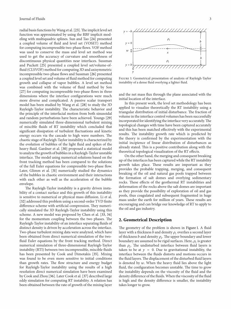
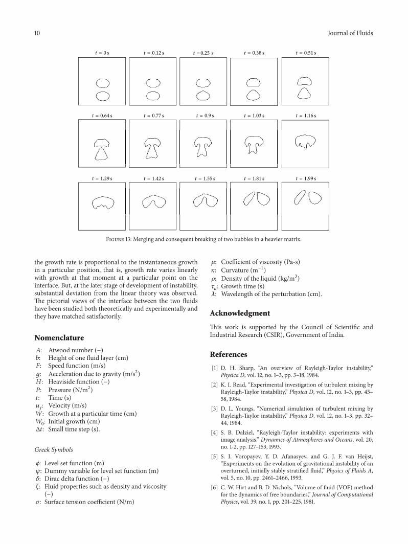
Related Documents