NUMERICAL ANALYSIS OF A FOUNDATION OF A WIND POWER …

Graz University of Technology

NUMERICAL ANALYSIS OF A FOUNDATION OF A WIND POWER PLANT

MASTER’S THESIS

Florian Moser

Institute of Soil Mechanics and Foundation Engineering Graz University of Technology

Advisors:

Ao.Univ.-Prof. Dipl.-Ing. Dr.techn. M.Sc. tit.Univ.-Prof. Helmut Schweiger


Dipl.-Ing. Dr.techn. Franz Tschuchnigg


Graz, September 2014

i

EIDESSTATTLICHE ERKLÄRUNG Ich erkläre an Eides statt, dass ich die vorliegende Arbeit selbstständig verfasst, andere als die angegebenen Quellen/Hilfsmittel nicht benutzt, und die den benutzten Quellen wörtlich und inhaltlich entnommenen Stellen als solche kenntlich gemacht habe. Graz, am

(Unterschrift)

STATUTORY DECLARATION I declare that I have authored this thesis independently, that I have not used other than the declared sources/resources, and that I have explicitly marked all material which has been quoted either literally or by content from the used sources.

Graz,

(signature)

ii

iii

Acknowledgements I like to take this opportunity to thank all the people who provided scientific, mental and financial support to make, not only this work, but my entire studies possible. I thank Prof. Helmut Schweiger who initiated and supervised this thesis and enabled the contact to Keller Grundbau Ges.m.b.H. Therefore I must also thank Dr. Václav Račanský and DI Laurentiu Floroiu who offered the documents of the practical project and gave me assistance during the development. A special gratitude goes to Dr. Franz Tschuchnigg for his dedication and the comprehensive support during the establishing of the present thesis. He was always accessible and provided me with constructive aspects and scientific discussions in several meetings. Furthermore I want to thank my family for the decent education and assistance they gave me in my whole life. They offered me mental and financial support over all these years and made my entire studies possible. Last but by no means least, my sincere thanks go to my good friends and especially to my girlfriend for their ongoing support and their constructive and motivating words throughout my education and beyond.

iv

v

Abstract To model the behaviour of a cemented material in numerical calculations more accurately, a material model [1] originally developed for modelling shotcrete, which is implemented in the finite element program Plaxis, has been used. Therefore the constitutive model considers, amongst others, effects like time dependent stiffness and strength of the material, and strain hardening and softening, to approximate fracture propagation through the material. In this work the shotcrete model has been used to model grouted stone columns of the foundation of a wind power plant. The investigations have been made in 2D with Plaxis 2D AE and in 3D with Plaxis 3D. Several studies, concerning both changes of material parameters and changes in the model geometry, were executed to analyse the effect of the constitutive model as well as various modelling assumptions on the behaviour of the entire structure. For determining the utilisation of the grouted stone columns in a conventional manner, normal forces in the columns, which have to be calculated from stresses in integration points, are required. While in 2D the Structural forces in volumes-tool provides accurate results when predicting the axial force of a soil cluster, the method of implementing a beam element within a three dimensional column cluster is only valid for plane cross sections and a linear stress distribution. Therefore both attempts have been reviewed by integrating stresses over the cross section. As a result, the implemented beam element predicts an inaccurate normal force due to the non-uniform stress distribution over the cross sections of the column, even for linear elastic soil clusters.

Kurzfassung Um das Materialverhalten von vermörtelten Säulen besser beschreiben zu können, wurde ein Materialmodell [1], ursprünglich entwickelt um Spritzbeton zu modellieren, welches in das Finite-Elemente-Programm Plaxis implementiert ist, verwendet. Das Stoffgesetz berücksichtigt unter anderem Eigenschaften wie die zeitabhängige Steifigkeit und Festigkeit, und die Ver- bzw. Entfestigung des Materials zufolge von Deformationen, um eine fortschreitende Rissbildung durch ein Material anzunähern. In dieser Arbeit wurde das shotcrete model verwendet, um zementierten Steinsäulen eines Fundaments einer Windkraftanlage zu modellieren. Die Berechnungen wurden in 2D mit Plaxis 2D AE und in 3D mit Plaxis 3D ausgeführt. Etliche Studien, mit Variation von Materialparametern und der Modellgeometrie, wurden durchgeführt, um sowohl den Effekt auf das Stoffgesetz, als auch den Effekt verschiedener Modellierungsannahmen auf das Verhalten der gesamten Struktur zu analysieren. Um die Ausnutzung der Steinsäulen auf konventionelle Weise zu bestimmen, werden die Normalkräfte in den Säulen, welche durch Integration der Spannungen in den Integrationspunkten berechnet werden müssen, benötigt. Während in 2D das Structural forces in volumes-Tool korrekte Ergebnisse für die axialen Kräfte eines Material-Clusters liefert, ist der Ansatz, ein Beam-Element in einen dreidimensionalen Volumenpfahl zu implementieren, nur für ebene Querschnitte und eine lineare Spannungsverteilung gültig. Folglich wurden beide Vorgehensweisen verglichen, indem die Spannungen über den Querschnitt integriert wurden. Es zeigt sich, dass das implementierte Beam-Element, aufgrund der ungleichmäßigen Spannungsverteilung über den Querschnitte des Pfahls, die Normalkraft, sogar für linear elastische Boden-Cluster, ungenau prognostiziert.

vi

vii

Table of contents

1. Introduction ................................................................................................................... 1

1.1. Background .................................................................................................................... 1

1.2. Numerical models .......................................................................................................... 2

1.3. Loading .......................................................................................................................... 3

2. Preliminary studies ........................................................................................................ 4

2.1. The normal forces by means of beam elements in soil clusters ................................... 4

3. The shotcrete model ..................................................................................................... 8

3.1. Constitutive model ........................................................................................................ 8

3.1.1. Compression hardening and softening ......................................................................... 8

3.1.2. Tension softening .......................................................................................................... 9

3.1.3. Time dependent material parameters .......................................................................... 9

3.1.4. Creep ........................................................................................................................... 12

3.1.5. Shrinkage ..................................................................................................................... 12

3.1.6. Safety factors ............................................................................................................... 12

3.2. Application of the shotcrete model............................................................................. 13

3.2.1. Default settings ........................................................................................................... 13

4. Calculations in 2D ........................................................................................................ 15

4.1. Calculations with column rows modelled in LE, MC and SC material model .............. 16

4.1.1. The approach of strain hardening and softening with the shotcrete model .............. 21

4.2. Parameter study with the shotcrete model ................................................................ 23

4.2.1. Stiffness ....................................................................................................................... 24

4.2.2. Strength ....................................................................................................................... 27

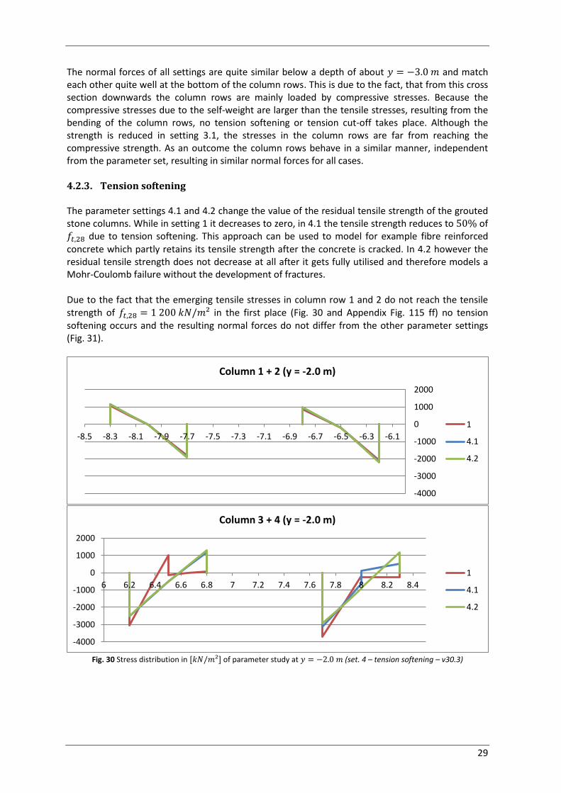
4.2.3. Tension softening ........................................................................................................ 29

4.2.4. Compression hardening and softening ....................................................................... 31

4.3. Different approaches concerning the model specifications ....................................... 34

4.3.1. Stabilized soil – Gravel or MIP-layer ............................................................................ 34

4.3.2. Design of the connection of the column heads with the foundation slab .................. 35

4.3.3. Variation of column length .......................................................................................... 38

4.3.4. Increase of the loading until failure occurs ................................................................. 41

4.3.5. Modelling of foundation slab and load application .................................................... 43

4.3.6. Comparison of stress integration, the structural forces in volumes-tool and beam

elements ...................................................................................................................... 45

5. Calculations in 3D ........................................................................................................ 48

viii

5.1. Overall behaviour ........................................................................................................ 50

5.2. Influence of the beam element on the model behaviour ........................................... 55

5.3. Rigid connection between foundation slab and grouted stone columns ................... 56

5.4. Increase of the loading ................................................................................................ 59

5.5. Stabilized soil – Gravel or MIP-layer ............................................................................ 62

5.6. Connection of the column heads with the foundation slab ........................................ 64

5.7. Calculations with the HSS material model and the power set to .................... 65

5.8. Calculations with the HS material model .................................................................... 68

6. Summary ...................................................................................................................... 70

References ........................................................................................................................................... 72

Appendix .............................................................................................................................................. 73

A.1. Determining the normal force of a volume column with Surfer 12 [7] ....................... 73

A.2. Soil parameters of Corbu 2 [3]..................................................................................... 76

A.3. List of investigated calculations ................................................................................... 81

A.4. Further calculation results ........................................................................................... 83

1

1. Introduction The main aspect of this thesis is the analysis of the foundation of a wind power plant on the basis of a realistic project employing the shotcrete material model [1] implemented in the FEM program Plaxis to model cemented columns. While the self-weight of a wind power plant is rather insignificant, the bending moment, resulting from the horizontal wind loads, is the decisive loading for the construction. Therefore, to transfer these forces into soft clayey subsoil, a concrete slab, founded on several drilled columns, serves as foundation of the turbine tower. The foundation slab has a circular shape and the columns, designed as grouted stone columns, are arranged in rows along the circumference of the slab. The specifications and parameters for the FEM-model are based on the expansion of Corbu 2 [3]. Two and three dimensional analyses are performed. Beside the total displacements and the settlements of the foundation, also the degree of utilisation of the bearing capacity of the construction was of interest. Therefore the grouted stone columns were modelled with the shotcrete material model to model the behaviour of the cemented columns more accurately. The constitutive model considers the effect of strain hardening and softening including tension softening thus initiation and propagation of cracks can be taken into account.

1.1. Background

Fig. 1 Vertical section in symmetrical plane

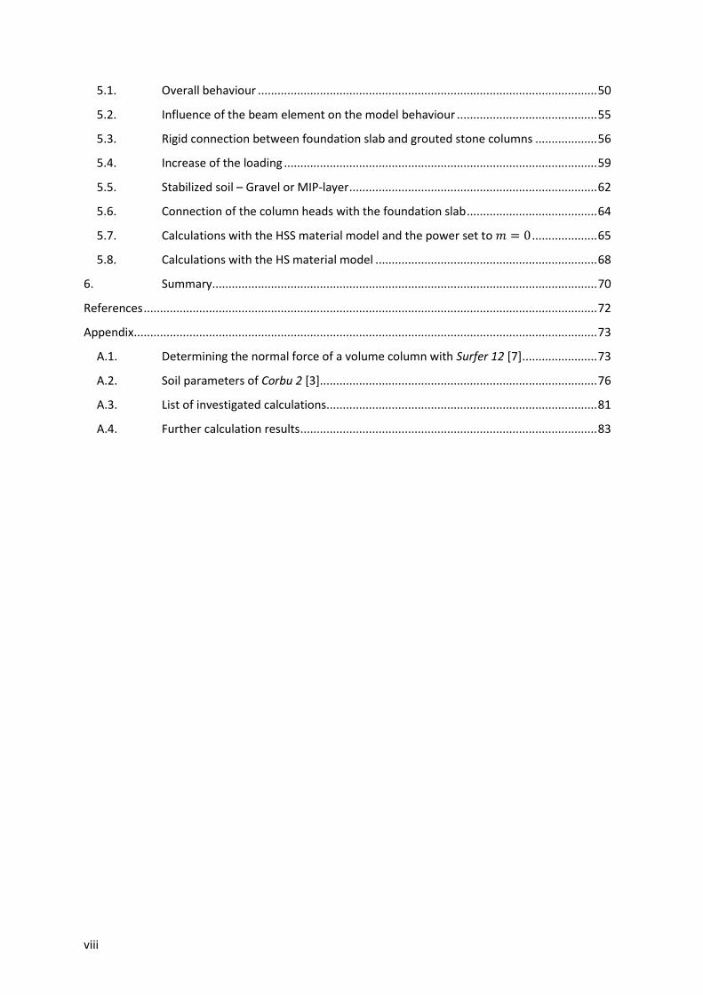
The expansion of the wind park Corbu 2 in Constanta County, Romania, which implies the construction of several Suzlon S88 HH 79.2 m turbines on soft soil, served as basis for the model. The foundation of one power plant consists of a circular concrete slab and three rows of grouted stone columns (Fig. 1 and Fig. 2) to transfer the load from the turbine tower into the ground. The columns are designed as predrilled cemented gravel columns and add up to a total of pieces for each turbine. Whereas the foundation slab is considered as concrete, the columns attain the properties of a concrete. The subsoil mainly consists of clay and is modelled with three

2

layers, on basis of the geotechnical report of the expansion of Corbu 2 [3]. The soil parameters are listed in Table 12 and are further investigated in chapter 5. No ground water was considered during most of the calculations. All investigations were executed with a predefined model, according to the mentioned references, regardless to safety factor analyses, improvement on the maximum utilisation or the optimisation of the economic efficiency of the construction.

Fig. 2 Plan view of foundation

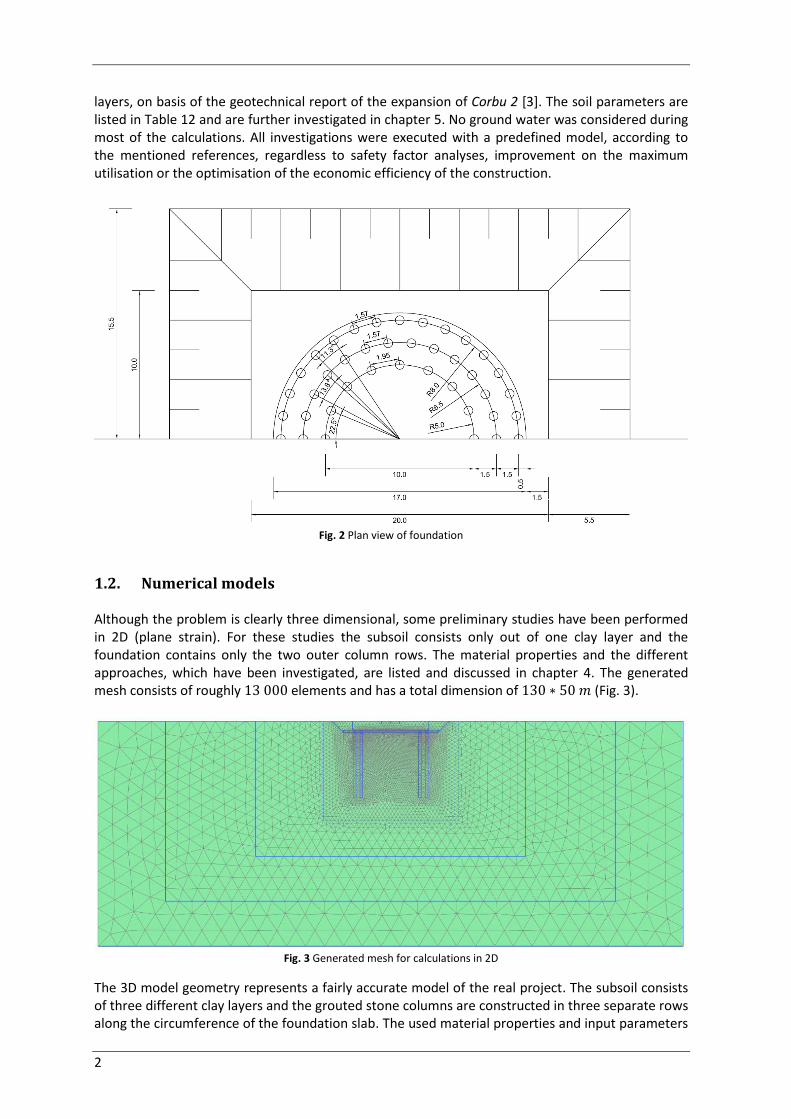
1.2. Numerical models Although the problem is clearly three dimensional, some preliminary studies have been performed in 2D (plane strain). For these studies the subsoil consists only out of one clay layer and the foundation contains only the two outer column rows. The material properties and the different approaches, which have been investigated, are listed and discussed in chapter 4. The generated mesh consists of roughly elements and has a total dimension of (Fig. 3).

Fig. 3 Generated mesh for calculations in 2D

The 3D model geometry represents a fairly accurate model of the real project. The subsoil consists of three different clay layers and the grouted stone columns are constructed in three separate rows along the circumference of the foundation slab. The used material properties and input parameters

3

are mentioned and explained in chapter 5. The generated mesh, shown in Fig. 4, consists of approximately elements and has a dimension of .

Fig. 4 Generated mesh for calculations in 3D

1.3. Loading To simplify the analysis, the turbine tower and therefore the loading on the foundation slab, are applied as point loads and force couple. The forces were derived from the design loads for the specific wind turbine [4], whereas only the maximum values of the load cases for typical operation situations in static conditions were assumed. To use the advantage of a symmetric model in the 3D calculations, only the resulting horizontal force and the bending moment were considered. No load out of the symmetrical plane or torsional moment was applied. The assumed forces for the 2D and the 3D model are shown in Table 1. Whereas the loads for the 3D model are already divided by two, due to the use of the symmetric subsystem, the values in 2D are adapted to produce approximately the same bearing pressure beneath the foundation slab.

Model geometry 3D 2D

Vertical force

Horizontal force

Bending moment

Table 1 Loading of the foundation slab for the 2D and 3D model

4

2. Preliminary studies

2.1. The normal forces by means of beam elements in soil clusters A very important aspect of the present thesis is the determination of the normal forces in columns, both in 2D and in 3D. While for 2D calculations Plaxis offers the useful tool “Structural forces in volumes” to readout the normal force, the shear force and the bending moment along a cross section line within a soil cluster (see chapter 4.3.6), for 3D investigation no such tool is available. Therefore the main approach to determine the normal force of a soil cluster is by implementing a beam element at the centre axis of the particular cluster. Via the beam element, which should have a very small Young’s modulus to minimize the influence on the model behaviour, the normal force can then be evaluated. In this case it has to be considered that the beam element represents a linear elastic rod that experiences the strains at the centre axis of the soil cluster. Therefore by dividing the resulting normal forces of the beam through the cross section area and the Young’s modulus of the beam element, the axial strains can be back calculated. From the obtained axial strains the normal force of the volume cluster can then be determined by multiplying the strains with the stiffness and the cross section area of the soil cluster. This method however assumes plane cross sections and a linear stress distribution. Hence the resulting normal forces may only be valid for a linear elastic soil cluster where the centre line of the stress distribution matches the beam element and the geometric axis of the cluster. Any mobilisation of the maximum material strength or cracking of the cross section narrows the linear elastic zone of the column down and affects the emerging normal forces. To compare the results of the investigation with beam elements, another method has been executed to calculate the normal forces of a column, modelled as soil cluster. In this case the stresses in the column’s axial direction of several cross sections in different depths have been integrated over the cross section area. Therefore also the fully mobilised or cracked zones are considered and the outcomes should predict more reliable results of the normal forces. For this investigation a simple 3D model of a single column, which is loaded by a surface load at the top, was generated (Fig. 5). The column reaches a depth of and has a diameter of . An interface element was placed around the column and a beam element was placed at the centre axis of the column.

Fig. 5 Generated mesh of single column, loaded with surface load (Single pile study 2)

5

The column was modelled both, with linear elastic (LE) and shotcrete (SC) material model, and is loaded with a circular surface load of . The surrounding subsoil consists of clay and has the same properties as the soil used in later calculations (see chapter 4). While the calculation of the normal forces with the beam element was executed as described before, the approach of the stress integration is explained in the following section (for a detailed guideline for the use of Surfer 12 see chapter A.1 in the Appendix). For investigation of the stresses in axial direction of the column, the Cartesian effective stresses of the soil cluster have been plotted (Fig. 7 – left) and exported into an Excel file. Due to an irregular arrangement of the stress points over the cross section of the column, several horizontal layers with a thickness of were extracted at different depths of the column. These values have then been processed with the mapping software Surfer 12 from Golden Software. The output of Plaxis specifies every stress point with its coordinates and the stresses. With Surfer 12 a three dimensional wireframe has then been generated, using the x- and y-coordinates for the position and the stress value for the altitude of the particular stress point (Fig. 6). This method therefore smears the stresses over the extracted layer, but the resulting deviation can be neglected due to the small thickness in comparison to the entire column length. A greater influence, which has to be considered, has the fact, that the stress points are always located within the cross section and hence no stress values at the edge of the column are listed in the output. Therefore Surfer 12 underestimates the area of the cross section, which can be indicated by the maximum dimensions of the wireframe in Fig. 6. As a result the volume under the wireframe, which can be determined with the program as well, delivers a slightly too low normal force. The mean stress value of the wireframe however can be used, and by multiplying it with the cross section area the axial force can be predicted quite accurately. This approach seems valid, also for nonlinear stress distributions over the cross section, because the gridding method, used by Surfer 12 to generate the three dimensional grid out of the Excel table, was set to “Natural neighbor”. This method weights the calculated average of after the local data density of the available values and therefore delivers the actual mean value, with no respect to the geometrical distribution over the cross section [7].

Fig. 6 Stress distribution over cross section at top of single column in SC, generated with Surfer (Single pile study 2)

6

Fig. 7 Left: Cartesian effective stresses of the column; right: effective normal stresses of interface at the bottom

of the column (Single pile study 2)

The calculated normal forces, both by using the beam element and by determining the mean axial stresses of the cross section with Surfer 12, are shown and compared in Fig. 8. With a diameter of the column has a cross section area of . Therefore the loading of generates a resulting normal force of approximately at the top of the column, which matches both approaches at the column’s head. Although the stress distribution does not emerge constant over the cross section (Fig. 6), Surfer 12 delivers an accurate mean stress value. The rough distribution of the wireframe results from the smearing of the stress values over the top layer and the irregular mesh of the soil cluster. With increasing depth however the two approaches calculate different values for the axial force, whereas the beam element predicts lower values than the stress integration. This follows from the uneven cross sections due to the skin friction at the surface of the column. To determine the resulting normal force at the base, the soil cluster and the interface at the bottom of the column have been investigated (Fig. 7 – right). With a mean stress value of about , the normal force calculates to approximately . While this value was predicted by executing the stress integration, the beam element underestimates the resulting force significantly. This follows from the stress distribution over the cross section at the bottom of the column. The interface shows a distribution similar to a Boussinesq distribution, which results from the reaction of the subsoil due to the load transfer. With the beam element located along the centre line of the soil cluster, it considers only the smaller stresses from the middle of the pressure bulb and therefore underestimates the emerging normal force. With an axial stress of roughly at the center line, according to the stress distribution at the bottom interface, the beam element should indicate a resulting force of approximately . Why, in this case, the normal force is predicted even lower, is not obvious and has not been investigated further.

7

In this case the calculations with a column in both linear elastic and shotcrete material model – the properties are adopted from the later calculation in chapter 4 – deliver exactly the same results (Fig. 8), because the stresses are far from reaching the material strength. Nevertheless it can be said, that great attention has to be paid, when beam elements are used to determine the axial force of a soil cluster. This method may only be valid for a linear stress distribution over the cross section, even by investigating a linear elastic soil cluster.

Fig. 8 Normal force over depth of single column modelled in LE (left) and SC (right) material model (Single pile study 2)

-10

-9

-8

-7

-6

-5

-4

-3

-2

-1

0

-300 -200 -100 0

De

pth

[m

]

Normal force [kN]

Single column - LE

Beam

Surfer

-10

-9

-8

-7

-6

-5

-4

-3

-2

-1

0

-300 -200 -100 0

De

pth

[m

]

Normal force [kN]

Single column - SC

Beam

Surfer

8

3. The shotcrete model

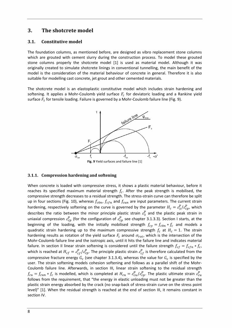
3.1. Constitutive model The foundation columns, as mentioned before, are designed as vibro replacement stone columns which are grouted with cement slurry during the construction process. To model these grouted stone columns properly the shotcrete model [1] is used as material model. Although it was originally created to simulate shotcrete linings in conventional tunnelling, the main benefit of the model is the consideration of the material behaviour of concrete in general. Therefore it is also suitable for modelling cast concrete, jet grout and other cemented materials. The shotcrete model is an elastoplastic constitutive model which includes strain hardening and softening. It applies a Mohr-Coulomb yield surface for deviatoric loading and a Rankine yield surface for tensile loading. Failure is governed by a Mohr-Coulomb failure line (Fig. 9).

Fig. 9 Yield surfaces and failure line [1]

3.1.1. Compression hardening and softening When concrete is loaded with compressive stress, it shows a plastic material behaviour, before it reaches its specified maximum material strength . After the peak strength is mobilised, the compressive strength decreases to a residual strength. The stress-strain curve can therefore be split up in four sections (Fig. 10), whereas , and are input parameters. The current strain

hardening, respectively softening on the curve is governed by the parameter

, which

describes the ratio between the minor principle plastic strain

and the plastic peak strain in

uniaxial compression

(for the configuration of

see chapter 3.1.3.3). Section I starts, at the

beginning of the loading, with the initially mobilised strength and models a

quadratic strain hardening up to the maximum compressive strength at . The strain hardening results as rotation of the yield surface around , which is the intersection of the Mohr-Coulomb failure line and the isotropic axis, until it hits the failure line and indicates material failure. In section II linear strain softening is considered until the failure strength ,

which is reached at

. The principle plastic strain

is therefore calculated from the

compressive fracture energy (see chapter 3.1.3.4), whereas the value for is specified by the user. The strain softening models cohesion softening and follows as a parallel shift of the Mohr-Coulomb failure line. Afterwards, in section III, linear strain softening to the residual strength

is modelled, which is completed at

. The plastic ultimate strain

follows from the requirement, that “the energy in elastic unloading must not be greater than the plastic strain energy absorbed by the crack (no snap-back of stress-strain curve on the stress point level)” [1]. When the residual strength is reached at the end of section III, it remains constant in section IV.

9

Fig. 10 Normalized stress-strain curve in compression [1]

3.1.2. Tension softening For tensile stresses the material behaviour of the shotcrete model is linear elastic until it reaches the specified maximum tensile strength . When the tensile strength is mobilised, linear strain softening occurs, which results in a parallel shift of the Rankine yield surface (Fig. 11). The strain

softening is governed by the parameter

, which indicates the ratio between the major

principle plastic strain

and the plastic ultimate strain in uniaxial tension

. The plastic ultimate

strain

is therefore calculated, similar to compression softening, from the tensile fracture energy (see chapter 3.1.3.4), which is an input parameter. The strain softening continues until the residual tensile strength is reached at . The residual value is therefore specified by the user. Afterwards the tensile strength remains constant and no further softening occurs.

Fig. 11 Tension softening on the yield surface (left) and on the normalized stress-strain curve in tension (right) [1]

The main advantage of the tension softening is the consideration of cracked concrete elements. Once the tensile strength is reached the remaining residual strength reduces to a smaller value, indicated by some reinforcement, or to zero to simulate an opening gap. 3.1.3. Time dependent material parameters The shotcrete lining in conventional tunnelling is loaded directly after construction and supports the rock mass already in its curing process. To model the change of the material properties and the deformation behaviour during concrete hydration, the shotcrete model implements time dependent parameters. Due to the fact that the grouted stone columns of the foundation in this paper are loaded a while after construction, and the cement slurry has time to harden, the time dependent material behaviour is not considered in this work. Therefore time dependency shall only be mentioned in the following sections for completeness.

10

3.1.3.1. Elastic stiffness During the hydration process the Young’s modulus of concrete increases with time. Therefore the shotcrete model considers a gaining elastic stiffness between the first hour after construction and the end of concrete curing past 28 days (Fig. 12). The Young’s modulus within the first hour and after 28 days is considered constant.

Fig. 12 Increase of the Young’s modulus over time [1]

Note that the input parameter respects the ratio of the elastic stiffness at a time of respectively days ( respectively hours), while the increase of the Young’s modulus is pursued after the first hour. 3.1.3.2. Compressive and tensile strength Similar to the stiffness, the material strength increases with concrete hardening over time. Therefore the input parameter indicates the ratio of the compressive strength at respectively days. The increase of the compressive strength results as a vertical shift of the Mohr-Coulomb failure line, while the inclination stays the same. The gain of the tensile strength follows the same procedure and is governed by a constant ratio of . Furthermore the values of , and remain constant over time.

The increase of the material strength of shotcrete is shown in Fig. 13, where rapid-hardening cement according to the early strength classes J1, J2 and J3 are used. Therefore the time scale does not fit the curing process of the grouted stone columns in this paper, but it shows the procedure applied by the shotcrete model.

Fig. 13 Increase of shotcrete strength with time [1]

11

3.1.3.3. Plastic deformability Young concrete has a low elastic stiffness and a high plastic ductility, which allows it to sustain large deformations, due to compressive stresses, at an early age. But with progressing hydration the stiffness increases and the ductility decreases over time. Therefore the shotcrete model

implements a compressive plastic peak strain

which is time dependent. The change of the

plastic peak strain follows a tri-linear function (Fig. 14) and considers the input values for

at a

time of , and hours. Within the first hour and after hours

remains constant.

Fig. 14 Reduction of

over time with

, and at , and hours [1]

3.1.3.4. Compressive and tensile fracture energy Both, the compressive and the tensile fracture energy , are input parameters for the cured concrete, whereas the change of the particular fracture energy over time is a result of the shotcrete model.

As shown before the compressive plastic peak strain

decreases with time. Because the ratio

is assumed to be constant, the compressive plastic failure strain

decreases as well and

as an outcome of this development the compressive fracture energy is reduced simultaneously.

While

is relatively large at the beginning, it drops rapidly in the first few hours of the concrete

age. Therefore the fracture energy has quite high values at first, due to the ductile behaviour,

but reduces significantly with

. The compressive material strength , on the other side,

increases over time, which leads to a higher . But because rises much slower, distributed over

the hydration process until the end at days, while

is constant after hours, the fracture

energy increases linear after the first drop until the maximum compressive strength is reached (Fig. 15).

Fig. 15 Stress-strain curves in uniaxial compression at different concrete ages (left) and development of compressive

fracture energy over compressive strength [1]

12

Because, other than for compressive stresses, the plastic deformability does not change for tensile

stress over time, the tensile failure strain

, which can be calculated from the tensile fracture energy , is assumed to be constant during concrete curing. As a result does not change due to change of ductile behaviour over time. But since the tensile strength increases until the end of hydration at days, the tensile fracture energy rises proportionally with (Fig. 16). Although this approach is slightly conservative, the linear increase of models general concrete behaviour reasonably well.

Fig. 16 Stress-strain curves in uniaxial tension at different concrete ages (left) and development of tensile fracture energy

over tensile strength [1]

3.1.4. Creep In the shotcrete model creep is considered viscoelastic, whereas it is implemented with a linear ratio between the creep strains and stress . Besides depends also on the elastic strains

by the creep factor . The development of the creep strains over time starts at the initiation of the loading at and is governed by the parameter

, which represents the time when of the creep strains have occurred. Creep has not been considered in the work presented here. 3.1.5. Shrinkage Shrinkage in the shotcrete model does not depend on the current stress state, but is modelled as

an isotropic volume loss over time. The shrinkage strains calculates from the final shrinkage

strains and the parameter

, which equals the time when of the shrinkage strains have taken place. Shrinkage has not been considered in the work presented here. 3.1.6. Safety factors To consider design values for the concrete strength, the safety factors

and

for both,

compressive and tensile strength separately, have been implemented in the shotcrete model. Because all calculations in this paper are executed using characteristic values (SLS analysis), both safety factors are considered as

.

13

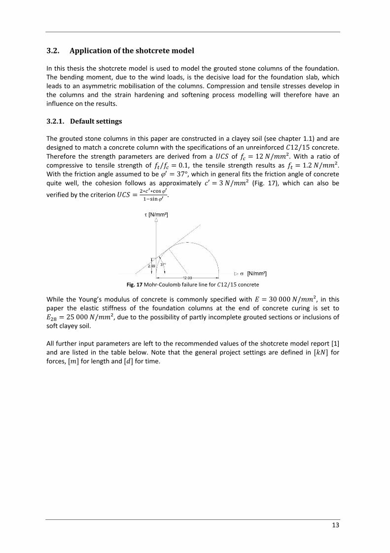
3.2. Application of the shotcrete model In this thesis the shotcrete model is used to model the grouted stone columns of the foundation. The bending moment, due to the wind loads, is the decisive load for the foundation slab, which leads to an asymmetric mobilisation of the columns. Compression and tensile stresses develop in the columns and the strain hardening and softening process modelling will therefore have an influence on the results. 3.2.1. Default settings The grouted stone columns in this paper are constructed in a clayey soil (see chapter 1.1) and are designed to match a concrete column with the specifications of an unreinforced concrete. Therefore the strength parameters are derived from a of . With a ratio of compressive to tensile strength of , the tensile strength results as . With the friction angle assumed to be , which in general fits the friction angle of concrete quite well, the cohesion follows as approximately (Fig. 17), which can also be

verified by the criterion

.

Fig. 17 Mohr-Coulomb failure line for concrete

While the Young’s modulus of concrete is commonly specified with , in this paper the elastic stiffness of the foundation columns at the end of concrete curing is set to , due to the possibility of partly incomplete grouted sections or inclusions of soft clayey soil. All further input parameters are left to the recommended values of the shotcrete model report [1] and are listed in the table below. Note that the general project settings are defined in for forces, for length and for time.

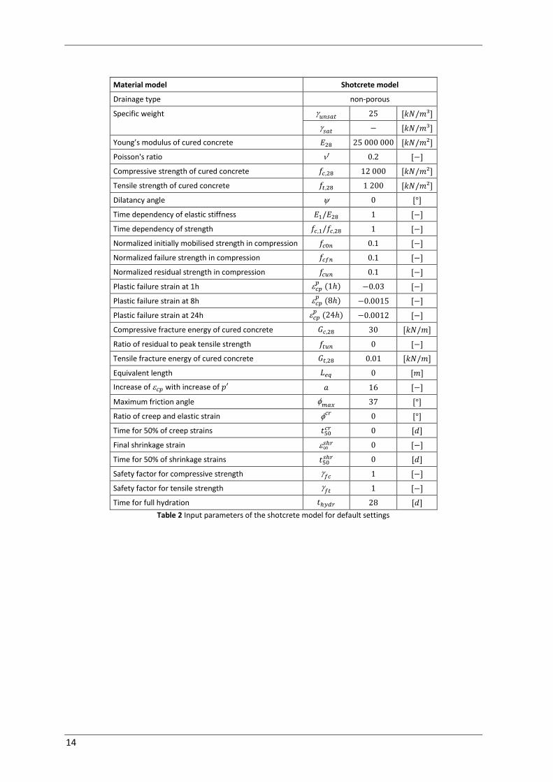
14

Material model Shotcrete model

Drainage type non-porous

Specific weight

Young’s modulus of cured concrete

Poisson's ratio

Compressive strength of cured concrete

Tensile strength of cured concrete

Dilatancy angle

Time dependency of elastic stiffness

Time dependency of strength

Normalized initially mobilised strength in compression

Normalized failure strength in compression

Normalized residual strength in compression

Plastic failure strain at 1h



Compressive fracture energy of cured concrete

Ratio of residual to peak tensile strength

Tensile fracture energy of cured concrete

Equivalent length

Increase of with increase of

Maximum friction angle

Ratio of creep and elastic strain

Time for 50% of creep strains

Final shrinkage strain

Time for 50% of shrinkage strains

Safety factor for compressive strength

Safety factor for tensile strength

Time for full hydration

Table 2 Input parameters of the shotcrete model for default settings

15

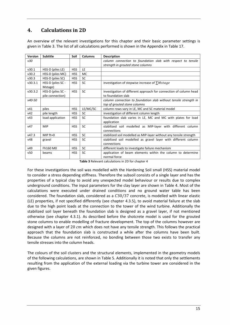
4. Calculations in 2D An overview of the relevant investigations for this chapter and their basic parameter settings is given in Table 3. The list of all calculations performed is shown in the Appendix in Table 17. Version Subtitle Soil Columns Description

v30 column connection to foundation slab with respect to tensile strength in grouted stone columns

v30.1 HSS-D (piles LE) HSS LE

v30.2 HSS-D (piles MC) HSS MC

v30.3 HSS-D (piles SC) HSS SC

v30.3.1 HSS-D (piles SC - Mstage)

HSS SC investigation of stepwise increase of

v30.3.2 HSS-D (piles SC - pile connection)

HSS SC investigation of different approach for connection of column head to foundation slab

v40-50 column connection to foundation slab without tensile strength in top of grouted stone columns

v41 piles HSS LE/MC/SC column rows vary in LE, MC and SC material model

v42 pile length HSS SC investigation of different column length

v43 load application HSS SC foundation slab varies in LE, MC and MC with plates for load application

v47 MIP HSS SC stabilized soil modelled as MIP-layer with different column connections

v47.3 MIP ft=0 HSS SC stabilized soil modelled as MIP-layer without any tensile strength

v48 gravel HSS SC stabilized soil modelled as gravel layer with different column connections

v49 Fh160 M0 HSS SC different loads to investigate failure mechanism

v50 beams HSS SC application of beam elements within the column to determine normal force

Table 3 Relevant calculations in 2D for chapter 4

For these investigations the soil was modelled with the Hardening Soil small (HSS) material model to consider a stress depending stiffness. Therefore the subsoil consists of a single layer and has the properties of a typical clay to avoid any unexpected model behaviour or results due to complex underground conditions. The input parameters for the clay layer are shown in Table 4. Most of the calculations were executed under drained conditions and no ground water table has been considered. The foundation slab, considered as a concrete, is modelled with linear elastic (LE) properties, if not specified differently (see chapter 4.3.5), to avoid material failure at the slab due to the high point loads at the connection to the tower of the wind turbine. Additionally the stabilized soil layer beneath the foundation slab is designed as a gravel layer, if not mentioned otherwise (see chapter 4.3.1). As described before the shotcrete model is used for the grouted stone columns to enable modelling of fracture development. The top of the columns however are designed with a layer of which does not have any tensile strength. This follows the practical approach that the foundation slab is constructed a while after the columns have been built. Because the columns are not reinforced, no bonding between those two exists to transfer any tensile stresses into the column heads. The colours of the soil clusters and the structural elements, implemented in the geometry models of the following calculations, are shown in Table 5. Additionally it is noted that only the settlements resulting from the application of the external loading via the turbine tower are considered in the given figures.

16

Material model HS small

Drainage type drained

Top level

Bottom level

Thickness

Specific weight

Stiffness

Power

Poisson's ratio

Reference pressure

Earth pressure coeff. in normal consolidation

Cohesion

Friction angle

Dilatancy angle

Shear strain

Shear modulus

Permeability

Interface strength

Earth pressure coeff. for initial stress state

Table 4 Input parameters for the subsoil in HSS-model for 2D calculations

Cluster/Element Material description Model Colour

Subsoil Clay HSS

Foundation slab Concrete LE/MC

Grouted stone columns Concrete LE/MC/SC

Concrete with SC

Stabilized soil Gravel MC

Mixed-in-place (MIP) layer MC

Interface adopted from subsoil HSS

Plate elastic steel rods Elastic

Table 5 Colours of the soil clusters and structural elements

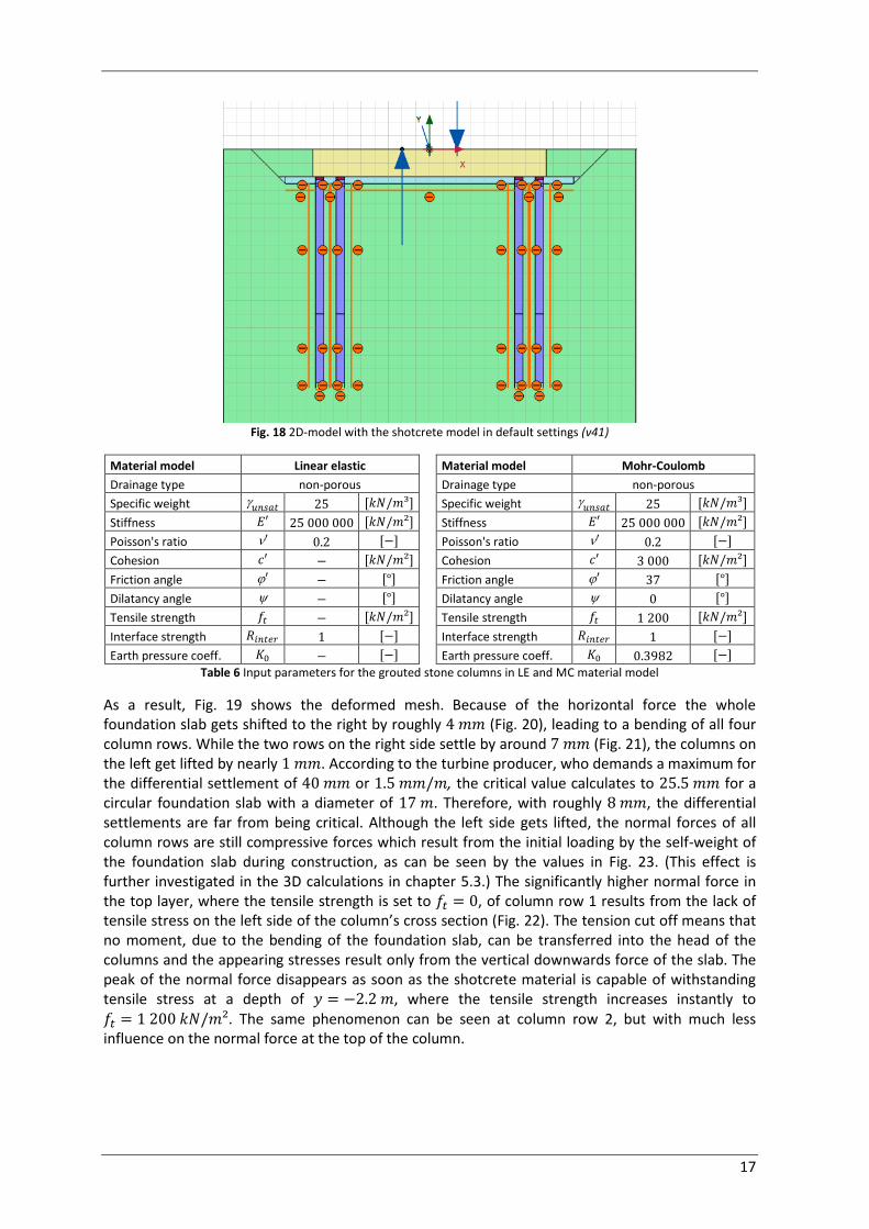
4.1. Calculations with column rows modelled in LE, MC and SC material model The geometry for the first calculations with the grouted stone columns modelled with the shotcrete model (SC) in the default settings (Table 2) is shown in Fig. 18. The top layer of the column heads have no tensile strength, , to neglect any transmission of tension, due to the missing bond between the columns and the foundation slab, as described before. The stabilized soil layer is modelled as gravel and drained conditions are assumed. With the same geometry and loading, calculations have been made where the columns were modelled with both, linear elastic (LE) and Mohr-Coulomb (MC) material models (Table 6), to compare the model behaviour and the normal forces of the columns with the shotcrete model (Fig. 23).

17

Fig. 18 2D-model with the shotcrete model in default settings (v41)

Material model Linear elastic


Specific weight

Stiffness

Poisson's ratio

Cohesion

Friction angle

Dilatancy angle

Tensile strength

Interface strength

Earth pressure coeff.

Material model Mohr-Coulomb


Specific weight

Stiffness

Poisson's ratio

Cohesion

Friction angle

Dilatancy angle

Tensile strength

Interface strength


Table 6 Input parameters for the grouted stone columns in LE and MC material model

As a result, Fig. 19 shows the deformed mesh. Because of the horizontal force the whole foundation slab gets shifted to the right by roughly (Fig. 20), leading to a bending of all four column rows. While the two rows on the right side settle by around (Fig. 21), the columns on the left get lifted by nearly . According to the turbine producer, who demands a maximum for the differential settlement of or , the critical value calculates to for a circular foundation slab with a diameter of . Therefore, with roughly , the differential settlements are far from being critical. Although the left side gets lifted, the normal forces of all column rows are still compressive forces which result from the initial loading by the self-weight of the foundation slab during construction, as can be seen by the values in Fig. 23. (This effect is further investigated in the 3D calculations in chapter 5.3.) The significantly higher normal force in the top layer, where the tensile strength is set to , of column row 1 results from the lack of tensile stress on the left side of the column’s cross section (Fig. 22). The tension cut off means that no moment, due to the bending of the foundation slab, can be transferred into the head of the columns and the appearing stresses result only from the vertical downwards force of the slab. The peak of the normal force disappears as soon as the shotcrete material is capable of withstanding tensile stress at a depth of , where the tensile strength increases instantly to . The same phenomenon can be seen at column row 2, but with much less influence on the normal force at the top of the column.

18

Fig. 19 Deformed mesh with shotcrete model in default settings (v41)

Fig. 20 Total displacements with shotcrete model in default settings (v41)

With the linear elastic columns, the normal forces in column 1 and 2 do not increase in the top layer at all (Fig. 23). This is based on to the fact that the tensile strength of a linear elastic material cannot be reduced to zero and therefore every rotation of the column’s cross section, because of asymmetric loading, generates tensile stresses instead of an opening gap. Furthermore, due to the linear elastic bond between the column and the foundation slab, the bending of the slab causes a moment transfer from the slab into the column rows. Consequently the maximum stresses, both compression and tensile stresses, in the top layer of the columns are much higher than with the use of the shotcrete model and tension cut off (Fig. 22). Because of the significant tension transmission at the connection of the column heads and the foundation slab, the values of the following stresses are not representative for the actual project settings, but it can be used to analyse the geometry model behaviour and allows some qualitative comparisons.

19

Fig. 21 Total displacements with shotcrete model in default settings (v41)

Fig. 22 Stress distribution in of column rows with linear elastic, Mohr-Coulomb and shotcrete material model at

(v41)

The normal force in the top layer of column row 4 however, is smaller with the shotcrete model, than with linear elastic material behaviour (Fig. 23). The stress distribution, with the peak stress not at the edge of the column, as shown in Fig. 22, seems to result from compression softening, but for this the compressive stress would have to exceed the compressive strength of the grouted stone columns. In this case the appearing stresses, even with linear elastic material behaviour, are with less than far from approaching the compressive strength of . This effect may follow from wrong stress interpolation, but it is not obvious where this behaviour derives from and further investigation would be necessary to analyse it.

-5000

-4000

-3000

-2000

-1000

0

1000

2000

-8.5 -8.3 -8.1 -7.9 -7.7 -7.5 -7.3 -7.1 -6.9 -6.7 -6.5 -6.3 -6.1

Column 1 + 2 (y = -2.05 m)

LE

MC

SC

-5000

-4000

-3000

-2000

-1000

0

1000

2000

6 6.2 6.4 6.6 6.8 7 7.2 7.4 7.6 7.8 8 8.2 8.4

Column 3 + 4 (y = -2.05 m)

LE

MC

SC

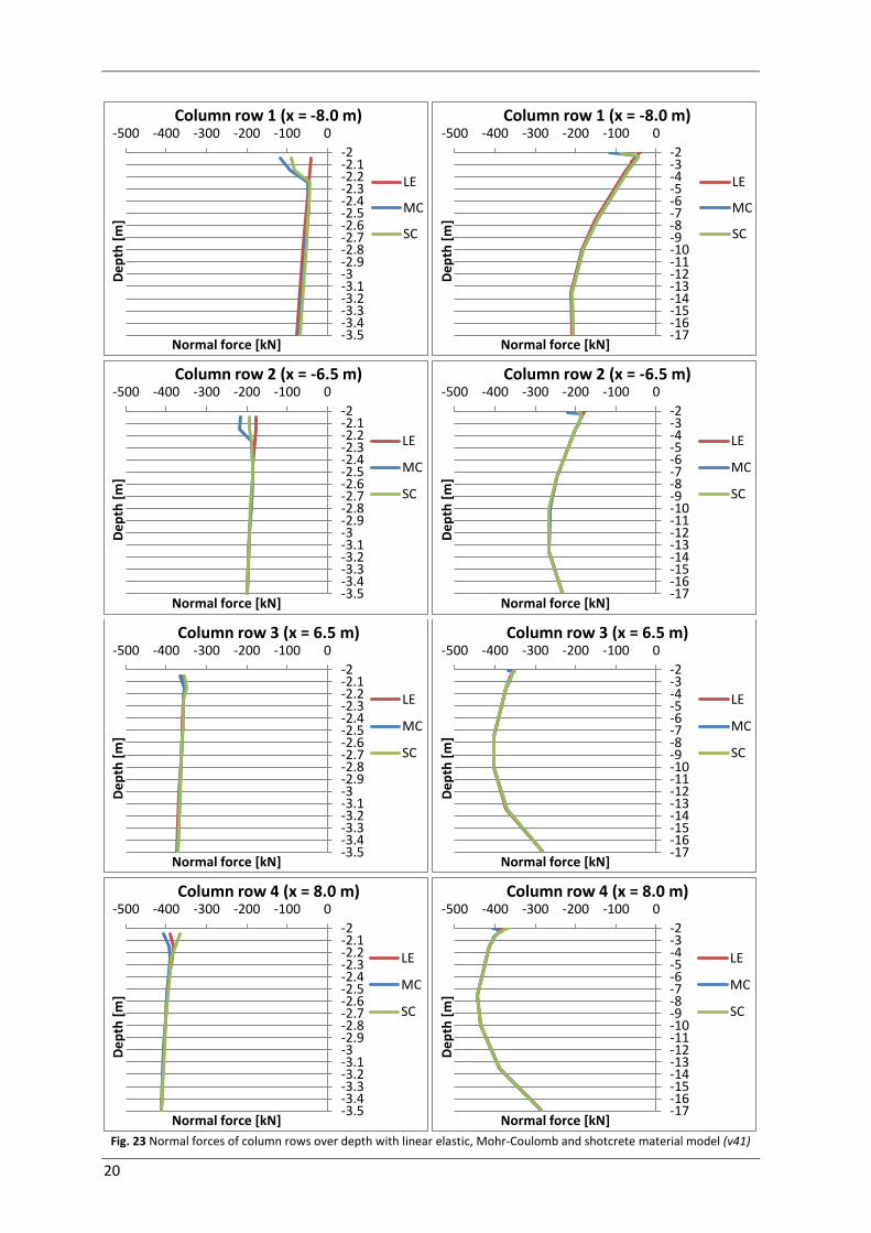
20

Fig. 23 Normal forces of column rows over depth with linear elastic, Mohr-Coulomb and shotcrete material model (v41)

-3.5-3.4-3.3-3.2-3.1-3-2.9-2.8-2.7-2.6-2.5-2.4-2.3-2.2-2.1-2

-500 -400 -300 -200 -100 0D

ep

th [

m]

Normal force [kN]

Column row 1 (x = -8.0 m)

LE

MC

SC

-17-16-15-14-13-12-11-10-9-8-7-6-5-4-3-2

-500 -400 -300 -200 -100 0

De

pth

[m

]

Normal force [kN]


LE

MC

SC

-3.5-3.4-3.3-3.2-3.1-3-2.9-2.8-2.7-2.6-2.5-2.4-2.3-2.2-2.1-2

-500 -400 -300 -200 -100 0

De

pth

[m

]

Normal force [kN]


LE

MC

SC

-17-16-15-14-13-12-11-10-9-8-7-6-5-4-3-2

-500 -400 -300 -200 -100 0

De

pth

[m

]

Normal force [kN]


LE

MC

SC

-3.5-3.4-3.3-3.2-3.1-3-2.9-2.8-2.7-2.6-2.5-2.4-2.3-2.2-2.1-2

-500 -400 -300 -200 -100 0

De

pth

[m

]

Normal force [kN]

Column row 3 (x = 6.5 m)

LE

MC

SC

-17-16-15-14-13-12-11-10-9-8-7-6-5-4-3-2

-500 -400 -300 -200 -100 0

De

pth

[m

]

Normal force [kN]


LE

MC

SC

-3.5-3.4-3.3-3.2-3.1-3-2.9-2.8-2.7-2.6-2.5-2.4-2.3-2.2-2.1-2

-500 -400 -300 -200 -100 0

De

pth

[m

]

Normal force [kN]


LE

MC

SC

-17-16-15-14-13-12-11-10-9-8-7-6-5-4-3-2

-500 -400 -300 -200 -100 0

De

pth

[m

]

Normal force [kN]


LE

MC

SC

21

On the one hand the vertical stresses of the column rows increase over depth due to their self-weight. On the other hand, due to the bending of the foundation slab under its self-weight, an asymmetric distribution of the compressive stresses emerges, which leads to a bending of the column rows. Additionally because of shift of the slab, the bending of the column rows increases and causes the normal force to get reduced in the upper part. Therefore the maximum resulting axial forces occurs in the lower, respectively middle part of the column rows. At the bottom of the columns the normal force however gets smaller due to the load transfer into the surrounding soil via skin friction. Nevertheless the calculations show that, when the tensile strength of the material is considered at a depth of , all three material models result in almost the same normal force in every column row. The stress distributions on the other hand are quite different at the upper part of the column rows, but also converge with depth and are quite congruent at and below (Appendix Fig. 103 ff). 4.1.1. The approach of strain hardening and softening with the shotcrete model To provoke the process of strain hardening and softening with the shotcrete model, calculations have been executed where the tensile strength of the grouted stone columns has not been reduced to zero at the connection to the foundation slab. Therefore tensile stresses and significantly higher compressive stresses, due to the bending of the slab, are transferred into the columns which partly exceed the strength of the material. For analysing the calculation process with respect to strain hardening and softening, the loading on the foundation slab was applied in steps of each by increasing the value by at a

time. The stress distribution of the cross sections at the top of the column rows at is shown in Fig. 24 for each step. While in column row 1 and 2 the emerging stresses do not approach to the compressive or tensile strength, respectively, the stresses at the outer edges of column row 3 and 4 exceed the tensile strength of the grouted stone columns of . In column row 3 the maximum tensile stress decreases once the loading passes ,

what means that tension softening takes place. The reduction of the tensile strength towards simulates a crack in the grouted stone column and therefore no tensile stresses can be transferred. Because the loading, and therefore the bending of the foundation slab, continues, the tensile section moves inwards into the intact area of the cross section at and

beyond. Because the compressive strength of on the other hand is by far not mobilised, no compression softening occurs and the maximum compressive stress rises until the end of loading at .

The same phenomenon can be seen in column row 4 where the tensile strength is already mobilised at the beginning of the loading at . The maximum tensile stresses

decrease and the tensile section moves inwards as discussed above. When the loading exceeds the tensile strength is fully mobilised in the middle of the column as well and the

tension softening process starts again, which means that the crack develops further through the column. At the end no more tensile stresses appear in column row 4. As before the compressive stresses do not reach the compressive strength and therefore no compression softening occurs. It has to be mentioned that the stresses were only evaluated at the edges and on both sides of the middle of the column’s cross section. Therefore the linear curve of the stress distribution is a result of linear interpolation. The phenomenon that the stresses at the right side of column row 4

22

temporarily indicate compression after tension softening occurred is due to false stress extrapolation and not quite accurate. The resulting stresses have to be zero due to the opening crack after exceeding the tensile strength.

Fig. 24 Stress distribution in at with increase of , with shotcrete material model (v30.3.1)

-4 000

-3 000

-2 000

-1 000

00

1 000

2 000

-8.5 -8.3 -8.1 -7.9 -7.7 -7.5 -7.3 -7.1 -6.9 -6.7 -6.5 -6.3 -6.1

Column 1 + 2 (y = -2.0 m)

0.1

0.2

0.3

0.4

0.5

∑Mstage

-4 000

-3 000

-2 000

-1 000

00

1 000

2 000

-8.5 -8.3 -8.1 -7.9 -7.7 -7.5 -7.3 -7.1 -6.9 -6.7 -6.5 -6.3 -6.1

Column 1 + 2 (y = -2.0 m)

0.6

0.7

0.8

0.9

1.0

∑Mstage

-4 000

-3 000

-2 000

-1 000

00

1 000

2 000

6 6.2 6.4 6.6 6.8 7 7.2 7.4 7.6 7.8 8 8.2 8.4

Column 3 + 4 (y = -2.0 m)

0.1

0.2

0.3

0.4

0.5

∑Mstage

-4 000

-3 000

-2 000

-1 000

00

1 000

2 000

6 6.2 6.4 6.6 6.8 7 7.2 7.4 7.6 7.8 8 8.2 8.4

Column 3 + 4 (y = -2.0 m)

0.6

0.7

0.8

0.9

1.0

∑Mstage

23

4.2. Parameter study with the shotcrete model To analyse the features of the shotcrete model [1] further, a parameter study has been executed. To disregard the lateral earth pressure on the foundation slab, due to the horizontal and vertical displacements of the construction, the soil clusters on both sides of the slab have not been activated during all calculations (Fig. 25). Furthermore in the top layer of the column rows a tensile strength of is considered, other than in the default settings (see chapter 3.2.1), to enhance the utilisation of the column rows and to be able to analyse the influence of the parameters concerning tensile strength and tension softening. The parameter input for the default settings is shown in Table 2. An overview of all analysed parameter changes is given in Table 7, whereat set 1 equals the default setting of the shotcrete model parameter. The general approach of the parameter study was not to vary the single parameters in the range of realistic values, concerning the used material for the columns, but to analyse their influence by a change in extent of a wide range.

Parameter set 1 2.1 2.2 3.1 3.2 3.3


Poisson's ratio



Dilatancy angle


Parameter set 1 4.1 4.2 5.1 5.2 5.3


Poisson's ratio



Dilatancy angle


Normalized initially mobilised strength in compression

Normalized failure strength in compression

Normalized residual strength in compression

Ratio of residual to peak tensile strength

Table 7 Different parameter sets for parameter study with shotcrete model (v30.3)

24

Fig. 25 Geometry for parameter study (v30.3)

4.2.1. Stiffness In the first calculations the stiffness of the column rows was set to and respectively. Due to the reduction of the stiffness the column rows have a smaller normal force in the column head (Fig. 27 – parameter set 2.1) and the pressure on the soil under the foundation slab increases, which leads to higher displacements. In contrast the normal force in the top of column row 1 and 2 is higher with setting 2.2, which can be explained by the higher attraction of stresses by stiffer elements. The exception of column row 3 is due to a reduction of the normal force in setting 1 and 2.2 at the column head. This decrease results from the higher tensile stresses in the cross section (Fig. 26), due to a higher bending moment, which comes from the rotation of the column head. The rotation of the column’s cross section results from the bending of the foundation slab and leads to higher tensile stresses the higher the stiffness of the column rows is. Therefore the normal force in setting 2.2 decreases the most at the column head, due to the highest stiffness. A similar approach can be made for column row 4. But in this case the tensile stresses at for the default settings are zero due to tension softening. Furthermore the stresses at the right side of the column indicate compression, which may be derived from false stress extrapolation. Therefore the resulting normal force is overestimated at the top of the column. With setting 2.2 however, because of the higher utilisation of the column head, even in the remaining intact cross section tensile stresses occur, which lower the resulting normal force. The deviation in normal forces at and results from less compressive stresses and not complete tension softening in the cross sections (Appendix Fig. 108 ff). But in general these values do not seem to be accurate because they would indicate a reduction of the normal force of about with setting 2.2 and even with setting 1, over a column length of . With a column’s surface area of , this amount cannot be dissipated by the skin friction of the column row in this small area. Furthermore the following increase of the normal force by roughly until cannot be definitely specified. It is not clearly determinable where this phenomenon comes from and would have to be investigated further in additional calculations.

25

The normal forces of parameter set 2.1 in the lower sections, from to the bottom of the column rows, match the default settings, which indicates a rather insignificant influence of the stiffness in the lower parts of the columns. The similar approach can also be investigated by the increase of in parameter set 2.2. Below the head of the column rows the normal forces are almost equal to the default settings and do not differ over depth. Additionally it has to be mentioned that great attention has to be paid, when forces are derived from the integration of the stresses over a cross section when strain hardening or softening occurs with the shotcrete model. While in general the method of stress integration matches the results of the Structural forces in volumes-tool in Plaxis quite well (see chapter 4.3.7), in this particular case the inter- and extrapolated stress distributions, as shown in Fig. 26 and the following, lead to inaccurate results. The normal forces of all column rows with setting 2.1, however, seem to be quiet accurate and have a relative constant value at the top of the column. This results from the low stiffness, where no strain hardening or softening takes place.

Fig. 26 Stress distribution in of parameter study at (set. 2 – stiffness – v30.3)

-4000

-3000

-2000

-1000

0

1000

2000

-8.5 -8.3 -8.1 -7.9 -7.7 -7.5 -7.3 -7.1 -6.9 -6.7 -6.5 -6.3 -6.1

Column 1 + 2 (y = -2.0 m)

1

2.1

2.2

-4000

-3000

-2000

-1000

0

1000

2000

6 6.2 6.4 6.6 6.8 7 7.2 7.4 7.6 7.8 8 8.2 8.4

Column 3 + 4 (y = -2.0 m)

1

2.1

2.2

26

Fig. 27 Normal forces of column rows over depth with different Young’s moduli (v30.3)

-3

-2.9

-2.8

-2.7

-2.6

-2.5

-2.4

-2.3

-2.2-2.1

-2

-800 -600 -400 -200 0D

ep

th [

m]

Normal force [kN]


1

2.1

2.2

-18

-16

-14

-12

-10

-8

-6

-4

-2

-800 -600 -400 -200 0

De

pth

[m

]

Normal force [kN]


1

2.1

2.2

-3

-2.9-2.8

-2.7

-2.6

-2.5

-2.4

-2.3

-2.2

-2.1

-2

-800 -600 -400 -200 0

De

pth

[m

]

Normal force [kN]


1

2.1

2.2

-18

-16

-14

-12

-10

-8

-6

-4

-2

-800 -600 -400 -200 0

De

pth

[m

]

Normal force [kN]


1

2.1

2.2

-3

-2.9

-2.8

-2.7

-2.6

-2.5

-2.4-2.3

-2.2

-2.1

-2

-800 -600 -400 -200 0

De

pth

[m

]

Normal force [kN]


1

2.1

2.2

-18

-16

-14

-12

-10

-8

-6

-4

-2

-800 -600 -400 -200 0

De

pth

[m

]

Normal force [kN]


1

2.1

2.2

-3

-2.9

-2.8

-2.7

-2.6

-2.5

-2.4

-2.3

-2.2

-2.1

-2

-800 -600 -400 -200 0

De

pth

[m

]

Normal force [kN]


1

2.1

2.2

-18

-16

-14

-12

-10

-8

-6

-4

-2

-800 -600 -400 -200 0

De

pth

[m

]

Normal force [kN]


1

2.1

2.2

27

4.2.2. Strength The next calculations were executed with different strength parameters. While the compressive and tensile strength were decreased and increased in the same ratio in setting 3.1 and 3.2, respectively, in setting 3.3 the compressive strength is set to default and no tensile strength is considered. While the normal forces in column row 1 and 2 seem to be quite independent from the strength parameters and therefore are similar to the default settings, the values of column row 3 and 4 face the same problems as described in the chapter before (Fig. 29). Because of this the axial forces may not be a good indicator for the influence of the strength parameters. But the stress distributions (Fig. 28 and Appendix Fig. 111 ff) allow some general conclusions to be drawn. The reduction of the strength parameter in setting 3.1 results in lower stresses, both compressive and tensile stress. Furthermore it changes the loading of the column heads of column row 3 and 4. Nearly the whole cross section is loaded with compressive stress. Whereas in other settings the outer part is loaded in tension or stresses are zero due to tension softening. An increase of the material strength in setting 3.2 on the other hand enhances the maximum stresses because no tension softening occurs in this case. A more or less elastic behaviour can be seen, which results in an almost linear stress distribution. By simply cutting off the tensile strength in setting 3.3, not only the tensile stresses, but also the compressive stresses are affected. While the tensile stresses are obviously zero, the compressive stresses are smaller and values are between setting 1 and 3.1. This indicates that because of the initial tensile strength in setting 1, a moment, resulting from the bending of the foundation slab, is transferred into the head of the column before tension softening takes place. Because of this greater compressive stresses develop, which partially remain when tension softening occurs. Therefore the maximum compressive stresses are higher than without an initial tensile strength.

Fig. 28 Stress distribution in of parameter study at (set. 3 – strength – v30.3)

-4000

-3000

-2000

-1000

0

1000

2000

-8.5 -8.3 -8.1 -7.9 -7.7 -7.5 -7.3 -7.1 -6.9 -6.7 -6.5 -6.3 -6.1

Column 1 + 2 (y = -2.0 m)

1

3.1

3.2

3.3

-4000

-3000

-2000

-1000

0

1000

2000

6 6.2 6.4 6.6 6.8 7 7.2 7.4 7.6 7.8 8 8.2 8.4

Column 3 + 4 (y = -2.0 m)

1

3.1

3.2

3.3

28

Fig. 29 Normal forces of column rows over depth with different strength parameters (v30.3)

-3

-2.9

-2.8

-2.7

-2.6

-2.5

-2.4

-2.3

-2.2-2.1

-2

-800 -600 -400 -200 0D

ep

th [

m]

Normal force [kN]


1

3.1

3.2

3.3

-18

-16

-14

-12

-10

-8

-6

-4

-2

-800 -600 -400 -200 0

De

pth

[m

]

Normal force [kN]


1

3.1

3.2

3.3

-3

-2.9-2.8

-2.7

-2.6

-2.5

-2.4

-2.3

-2.2

-2.1

-2

-800 -600 -400 -200 0

De

pth

[m

]

Normal force [kN]


1

3.1

3.2

3.3

-18

-16

-14

-12

-10

-8

-6

-4

-2

-800 -600 -400 -200 0

De

pth

[m

]

Normal force [kN]


1

3.1

3.2

3.3

-3

-2.9

-2.8

-2.7

-2.6

-2.5

-2.4-2.3

-2.2

-2.1

-2

-800 -600 -400 -200 0

De

pth

[m

]

Normal force [kN]


1

3.1

3.2

3.3

-18

-16

-14

-12

-10

-8

-6

-4

-2

-800 -600 -400 -200 0

De

pth

[m

]

Normal force [kN]


1

3.1

3.2

3.3

-3

-2.9

-2.8

-2.7

-2.6

-2.5

-2.4

-2.3

-2.2

-2.1

-2

-800 -600 -400 -200 0

De

pth

[m

]

Normal force [kN]


1

3.1

3.2

3.3

-18

-16

-14

-12

-10

-8

-6

-4

-2

-800 -600 -400 -200 0

De

pth

[m

]

Normal force [kN]


1

3.1

3.2

3.3

29

The normal forces of all settings are quite similar below a depth of about and match each other quite well at the bottom of the column rows. This is due to the fact, that from this cross section downwards the column rows are mainly loaded by compressive stresses. Because the compressive stresses due to the self-weight are larger than the tensile stresses, resulting from the bending of the column rows, no tension softening or tension cut-off takes place. Although the strength is reduced in setting 3.1, the stresses in the column rows are far from reaching the compressive strength. As an outcome the column rows behave in a similar manner, independent from the parameter set, resulting in similar normal forces for all cases. 4.2.3. Tension softening The parameter settings 4.1 and 4.2 change the value of the residual tensile strength of the grouted stone columns. While in setting 1 it decreases to zero, in 4.1 the tensile strength reduces to of due to tension softening. This approach can be used to model for example fibre reinforced concrete which partly retains its tensile strength after the concrete is cracked. In 4.2 however the residual tensile strength does not decrease at all after it gets fully utilised and therefore models a Mohr-Coulomb failure without the development of fractures. Due to the fact that the emerging tensile stresses in column row 1 and 2 do not reach the tensile strength of in the first place (Fig. 30 and Appendix Fig. 115 ff) no tension softening occurs and the resulting normal forces do not differ from the other parameter settings (Fig. 31).

Fig. 30 Stress distribution in of parameter study at (set. 4 – tension softening – v30.3)

-4000

-3000

-2000

-1000

0

1000

2000

-8.5 -8.3 -8.1 -7.9 -7.7 -7.5 -7.3 -7.1 -6.9 -6.7 -6.5 -6.3 -6.1

Column 1 + 2 (y = -2.0 m)

1

4.1

4.2

-4000

-3000

-2000

-1000

0

1000

2000

6 6.2 6.4 6.6 6.8 7 7.2 7.4 7.6 7.8 8 8.2 8.4

Column 3 + 4 (y = -2.0 m)

1

4.1

4.2

30

Fig. 31 Normal forces of column rows over depth with different tension softening (v30.3)

-3

-2.9

-2.8

-2.7

-2.6

-2.5

-2.4

-2.3

-2.2-2.1

-2

-800 -600 -400 -200 0D

ep

th [

m]

Normal force [kN]


1

4.1

4.2

-18

-16

-14

-12

-10

-8

-6

-4

-2

-800 -600 -400 -200 0

De

pth

[m

]

Normal force [kN]


1

4.1

4.2

-3

-2.9-2.8

-2.7

-2.6

-2.5

-2.4

-2.3

-2.2

-2.1

-2

-800 -600 -400 -200 0

De

pth

[m

]

Normal force [kN]


1

4.1

4.2

-18

-16

-14

-12

-10

-8

-6

-4

-2

-800 -600 -400 -200 0

De

pth

[m

]

Normal force [kN]


1

4.1

4.2

-3

-2.9

-2.8

-2.7

-2.6

-2.5

-2.4-2.3

-2.2

-2.1

-2

-800 -600 -400 -200 0

De

pth

[m

]

Normal force [kN]


1

4.1

4.2

-18

-16

-14

-12

-10

-8

-6

-4

-2

-800 -600 -400 -200 0

De

pth

[m

]

Normal force [kN]


1

4.1

4.2

-3

-2.9

-2.8

-2.7

-2.6

-2.5

-2.4

-2.3

-2.2

-2.1

-2

-800 -600 -400 -200 0

De

pth

[m

]

Normal force [kN]


1

4.1

4.2

-18

-16

-14

-12

-10

-8

-6

-4

-2

-800 -600 -400 -200 0

De

pth

[m

]

Normal force [kN]


1

4.1

4.2

31

In column row 3 the tensile strength is fully mobilised at the right edge of the column’s head and therefore tension softening takes place. With a reduction of the residual strength to zero in setting 1 the softening develops further inwards along the cross section due to the redistribution of the tensile stresses. With setting 4.1 however, where the tensile strength decreases only to of the maximum, the stress redistribution affects a much smaller area and tension softening occurs only on the outer edge of the top of the column row. Therefore the stress distribution over the cross section is almost equal to setting 4.2, where no softening takes place, and results in a similar normal force. Because column row 4 is again the most loaded one, the effect of strain softening can be investigated rather well. With setting 1 the tensile zone at the top of the column is fully cracked and slight compression occurs due to the false extrapolation of the stresses, which overestimates the normal force. Stresses of the remaining intact cross section are compressive without any tension at all. Similar to this the partial reduction of the residual tensile strength in setting 4.1 leads to an almost constant stress level at residual level in the tensile zone. This is again because of the proceeding cracking of the cross section, although it retains of its tensile strength. When no tension softening is considered in setting 4.2, the stress distribution is rather linear over the cross section. The maximum compressive stresses however are slightly less than compared to tension softening, which results from the larger compressive zone due to the fully intact cross section. Therefore the moment from the rotation of the column’s cross section, initiated by the bending of the foundation slab, can be carried by a larger area and therefore result in smaller maximum stresses. The consideration of this effect can be very important when, unlike to this case, the compressive strength for example is almost fully mobilised in calculations with a Mohr-Coulomb material model. The approach of the shotcrete model with tension softening reduces the intact cross section and increases the compressive stresses further. Therefore compression softening would occur additionally and the element would probably fail. 4.2.4. Compression hardening and softening The final calculations of the parameter study were executed with respect to compression softening and hardening. While in setting 5.1 the initially mobilised compressive strength is already equal to the maximum compressive strength , which neglects compression hardening, in setting 5.2 and 5.3 the compressive failure strength and the compressive residual strength are higher than in the default settings, which change the process of compression softening. Once again column row 1 and 2 are not affected neither by compression nor tension softening and therefore have a similar stress distribution (Fig. 32 and Appendix Fig. 119 ff) and resulting normal force (Fig. 33), independent from the applied parameter settings. In column row 3 and 4 however the increase of the initially mobilised compressive strength in setting 5.1 changes the shape of the stress distribution over the cross section at the top of the columns. While tension softening occurs as well as with the default settings in the tensile zone, in column row 3 the intact area does not bear any tensile stresses and is now completely loaded with compressive stresses. This results in a higher normal force in the head of the column, although the maximum compressive stress is smaller. On the contrary in column row 4, where no more tension occurred, the maximum compressive stress appears significantly higher than with default settings at the top of the column. Whereas in setting 1 compression hardening takes place as soon as of the maximum compressive strength is mobilised, no strain hardening is considered in

setting 5.1. Therefore the compressive strength is already at its maximum, even for small strains, which results in linear elastic material behaviour during load application. So no plastic hardening occurs, because higher stresses can already be sustained in the first place. According to this the

32

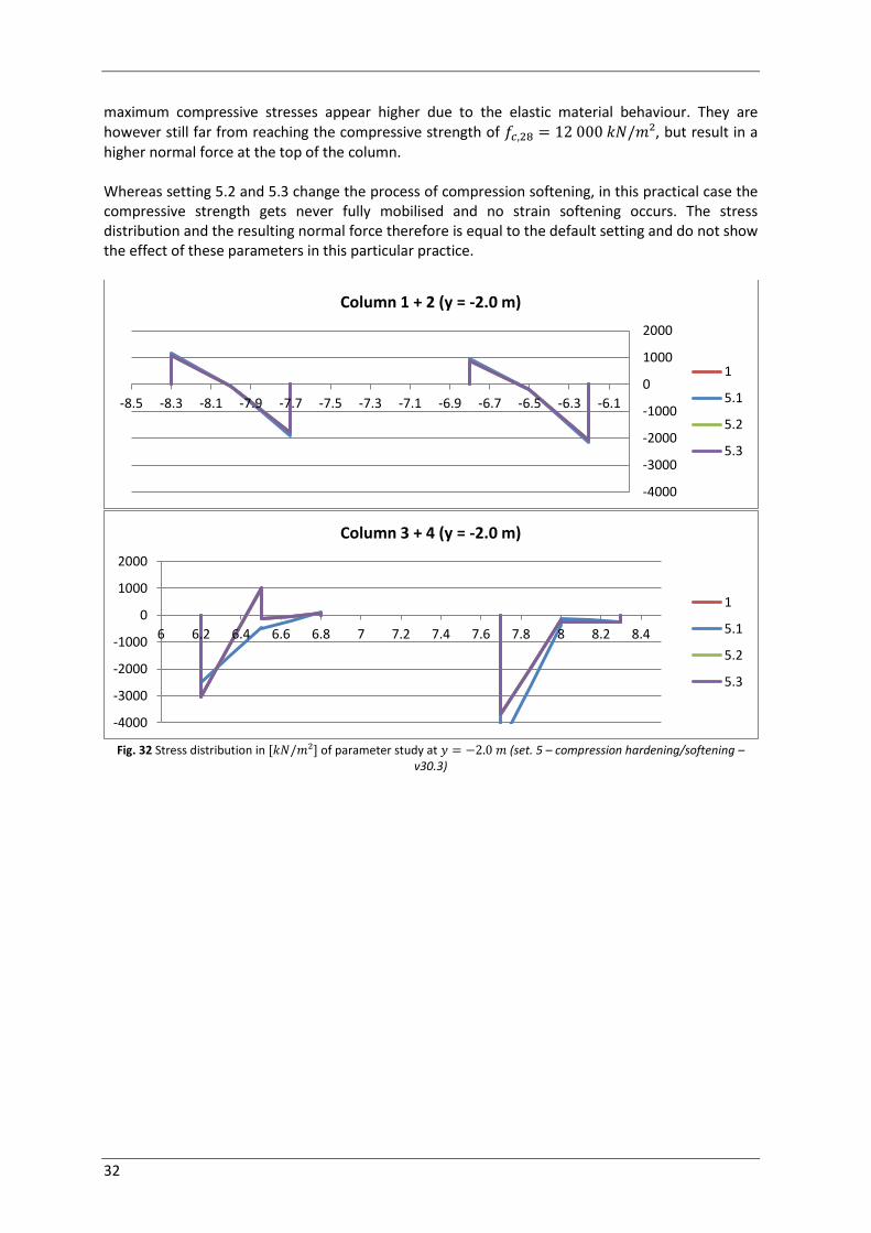
maximum compressive stresses appear higher due to the elastic material behaviour. They are however still far from reaching the compressive strength of , but result in a higher normal force at the top of the column. Whereas setting 5.2 and 5.3 change the process of compression softening, in this practical case the compressive strength gets never fully mobilised and no strain softening occurs. The stress distribution and the resulting normal force therefore is equal to the default setting and do not show the effect of these parameters in this particular practice.

Fig. 32 Stress distribution in of parameter study at (set. 5 – compression hardening/softening –

v30.3)

-4000

-3000

-2000

-1000

0

1000

2000

-8.5 -8.3 -8.1 -7.9 -7.7 -7.5 -7.3 -7.1 -6.9 -6.7 -6.5 -6.3 -6.1

Column 1 + 2 (y = -2.0 m)

1

5.1

5.2

5.3

-4000

-3000

-2000

-1000

0

1000

2000

6 6.2 6.4 6.6 6.8 7 7.2 7.4 7.6 7.8 8 8.2 8.4

Column 3 + 4 (y = -2.0 m)

1

5.1

5.2

5.3

33

Fig. 33 Normal forces of column rows over depth with different compression hardening/softening (v30.3)

-3

-2.9

-2.8

-2.7

-2.6

-2.5

-2.4

-2.3

-2.2-2.1

-2

-1000 -800 -600 -400 -200 0D

ep

th [

m]

Normal force [kN]


1

5.1

5.2

5.3

-18

-16

-14

-12

-10

-8

-6

-4

-2

-1000 -800 -600 -400 -200 0

De

pth

[m

]

Normal force [kN]


1

5.1

5.2

5.3

-3

-2.9-2.8

-2.7

-2.6

-2.5

-2.4

-2.3

-2.2

-2.1

-2

-1000 -800 -600 -400 -200 0

De

pth

[m

]

Normal force [kN]


1

5.1

5.2

5.3

-18

-16

-14

-12

-10

-8

-6

-4

-2

-1000 -800 -600 -400 -200 0

De

pth

[m

]

Normal force [kN]


1

5.1

5.2

5.3

-3

-2.9

-2.8

-2.7

-2.6

-2.5

-2.4-2.3

-2.2

-2.1

-2

-1000 -800 -600 -400 -200 0

De

pth

[m

]

Normal force [kN]


1

5.1

5.2

5.3

-18

-16

-14

-12

-10

-8

-6

-4

-2

-1000 -800 -600 -400 -200 0

De

pth

[m

]

Normal force [kN]


1

5.1

5.2

5.3

-3

-2.9

-2.8

-2.7

-2.6

-2.5

-2.4

-2.3

-2.2

-2.1

-2

-1000 -800 -600 -400 -200 0

De

pth

[m

]

Normal force [kN]


1

5.1

5.2

5.3

-18

-16

-14

-12

-10

-8

-6

-4

-2

-1000 -800 -600 -400 -200 0

De

pth

[m

]

Normal force [kN]


1

5.1

5.2

5.3

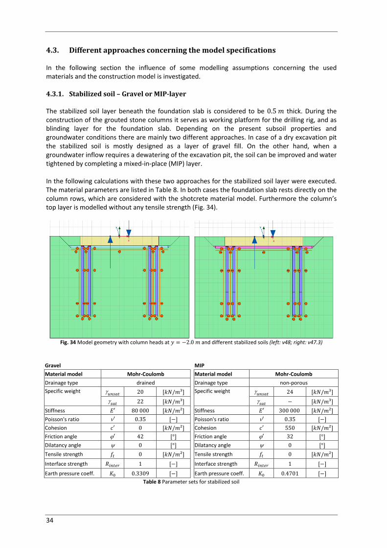
34

4.3. Different approaches concerning the model specifications In the following section the influence of some modelling assumptions concerning the used materials and the construction model is investigated. 4.3.1. Stabilized soil – Gravel or MIP-layer The stabilized soil layer beneath the foundation slab is considered to be thick. During the construction of the grouted stone columns it serves as working platform for the drilling rig, and as blinding layer for the foundation slab. Depending on the present subsoil properties and groundwater conditions there are mainly two different approaches. In case of a dry excavation pit the stabilized soil is mostly designed as a layer of gravel fill. On the other hand, when a groundwater inflow requires a dewatering of the excavation pit, the soil can be improved and water tightened by completing a mixed-in-place (MIP) layer. In the following calculations with these two approaches for the stabilized soil layer were executed. The material parameters are listed in Table 8. In both cases the foundation slab rests directly on the column rows, which are considered with the shotcrete material model. Furthermore the column’s top layer is modelled without any tensile strength (Fig. 34).

Fig. 34 Model geometry with column heads at and different stabilized soils (left: v48; right: v47.3)

Gravel


Drainage type drained

Specific weight

Stiffness

Poisson's ratio

Cohesion

Friction angle

Dilatancy angle

Tensile strength

Interface strength


MIP



Specific weight

Stiffness

Poisson's ratio

Cohesion

Friction angle

Dilatancy angle

Tensile strength

Interface strength


Table 8 Parameter sets for stabilized soil

35

Due to the thin layer and the low stiffness of the stabilized soil, regardless of gravel or MIP-layer, compared to the grouted stone columns, which have a Young’s modulus of , the influence on the normal forces of the column rows is rather insignificant (Fig. 35). Therefore it can be said, that the choice of the material of the stabilized soil will not be of great relevance as far as the overall behaviour is concerned.

Fig. 35 Normal forces of column rows over depth with different stabilized soils (v47.3 and v48)

4.3.2. Design of the connection of the column heads with the foundation slab Another design approach of the foundation, compared to the settings in chapter 4.3.1, can be where the top of the grouted stone columns are not connected directly to the foundation slab, but are placed at the bottom side of the stabilized soil layer (Fig. 39). The total settlements of the foundation are calculated a little higher, because the slab does not rest on the top of the columns but on the stabilized soil, which has a smaller stiffness in comparison to the columns. The advantage of this design though is the more evenly loading of the column heads. In general the normal forces in the upper part of the column rows are slightly smaller when the column heads are located below the stabilized soil layer (Fig. 36) because more of the load is distributed by the higher bearing pressure through the gravel or MIP-layer. The exception of column row 1 is due to the smaller displacement of the column head, when it is not directly connected to the foundation slab. Because of the smaller horizontal shift, the top of the column gets pulled out less than before which preserves a higher compressive force in the column. Furthermore no tensile stresses, due to the bending of the foundation slab, occur at the column’s head anymore and the cross section is evenly loaded with compressive stresses. Over depth the normal forces of both approaches converge to each other.

-3-2.9

-2.8

-2.7

-2.6

-2.5

-2.4

-2.3

-2.2

-2.1

-2

-500 -400 -300 -200 -100 0

De

pth

[m

]

Normal force [kN]


Gravel

MIP

-3-2.9

-2.8

-2.7

-2.6

-2.5

-2.4

-2.3

-2.2

-2.1

-2

-500 -400 -300 -200 -100 0

De

pth

[m

] Normal force [kN]


Gravel

MIP

-3-2.9

-2.8

-2.7

-2.6

-2.5-2.4

-2.3

-2.2

-2.1

-2

-500 -400 -300 -200 -100 0

De

pth

[m

]

Normal force [kN]


Gravel

MIP

-3-2.9

-2.8

-2.7

-2.6

-2.5-2.4

-2.3

-2.2

-2.1

-2

-500 -400 -300 -200 -100 0

De

pth

[m

]

Normal force [kN]


Gravel

MIP

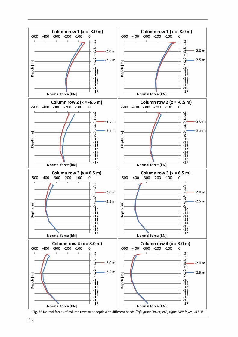
36

Fig. 36 Normal forces of column rows over depth with different heads (left: gravel layer, v48; right: MIP-layer, v47.3)

-17-16-15-14-13-12-11-10-9-8-7-6-5-4-3-2

-500 -400 -300 -200 -100 0D

ep

th [

m]

Normal force [kN]


-2.0 m

-2.5 m

-17-16-15-14-13-12-11-10-9-8-7-6-5-4-3-2

-500 -400 -300 -200 -100 0

De

pth

[m

]

Normal force [kN]


-2.0 m

-2.5 m

-17-16-15-14-13-12-11-10-9-8-7-6-5-4-3-2

-500 -400 -300 -200 -100 0

De

pth

[m

]

Normal force [kN]


-2.0 m

-2.5 m

-17-16-15-14-13-12-11-10-9-8-7-6-5-4-3-2

-500 -400 -300 -200 -100 0

De

pth

[m

]

Normal force [kN]


-2.0 m

-2.5 m

-17-16-15-14-13-12-11-10-9-8-7-6-5-4-3-2

-500 -400 -300 -200 -100 0

De

pth

[m

]

Normal force [kN]


-2.0 m

-2.5 m

-17-16-15-14-13-12-11-10-9-8-7-6-5-4-3-2

-500 -400 -300 -200 -100 0

De

pth

[m

]

Normal force [kN]


-2.0 m

-2.5 m

-17-16-15-14-13-12-11-10-9-8-7-6-5-4-3-2

-500 -400 -300 -200 -100 0

De

pth

[m

]

Normal force [kN]


-2.0 m

-2.5 m

-17-16-15-14-13-12-11-10-9-8-7-6-5-4-3-2

-500 -400 -300 -200 -100 0

De

pth

[m

]

Normal force [kN]


-2.0 m

-2.5 m

37

Fig. 37 Stress distribution in with a gravel-layer and different height of column heads at (v48)

Fig. 38 Stress distribution in with a gravel-layer and different height of column heads at (v48)

-2000

-1500

-1000

-500

0

500

1000

-8.5 -8.3 -8.1 -7.9 -7.7 -7.5 -7.3 -7.1 -6.9 -6.7 -6.5 -6.3 -6.1

Column 1 + 2 (y = -2.05 m)

-2.0 m

-2.5 m

-2000

-1500

-1000

-500

0

500

1000

6 6.2 6.4 6.6 6.8 7 7.2 7.4 7.6 7.8 8 8.2 8.4

Column 3 + 4 (y = -2.05 m)

-2.0 m

-2.5 m

-2000

-1500

-1000

-500

0

500

1000

-8.5 -8.3 -8.1 -7.9 -7.7 -7.5 -7.3 -7.1 -6.9 -6.7 -6.5 -6.3 -6.1

Column 1 + 2 (y = -2.55 m)

-2.0 m

-2.5 m

-2000

-1500

-1000

-500

0

500

1000

6 6.2 6.4 6.6 6.8 7 7.2 7.4 7.6 7.8 8 8.2 8.4

Column 3 + 4 (y = -2.55 m)

-2.0 m

-2.5 m

38

Fig. 39 Model geometry with column heads at and different stabilized soils (left: v48; right: v47.3)

The stress distributions over the cross section of the column rows however are different, depending on the height of the column head (Fig. 37 and Fig. 38). With the top of the column rows at , i.e. when they are directly connected to the foundation slab, much higher compressive stresses occur due to the high Young’s modulus of both materials. Otherwise, with the column heads at , the stress distribution in the stabilized soil layer is almost constant, with lower maximum stresses. At the top of the lower column rows, indicated by the cross section at , the stress distribution shows a pressure bulb similar to the Boussinesq distribution. Therefore only compressive stresses develop and once again the maximum stresses are smaller. This obviously is in favour for cemented materials because of the higher compressive than tensile strength. Furthermore no tension softening occurs which benefits the persistence of the grouted stone columns. The difference between the approach of the gravel or the MIP-layer is again quite small. It is noticeable though, that because of the higher stiffness the columns with the head at experience more loading from the MIP-layer than from the gravel layer. 4.3.3. Variation of column length To investigate a more economical construction, the length of the column rows has been be decreased. A simple reduction of the number of columns, regarding to a 3D model (see chapter 1.1), will reduce the stability of the structure, due to the high pressure at the top of the columns and due to the high loading from the wind, which can strike from any direction. Therefore to decrease the quantity of drilled column meters, shorter columns can be constructed. This approach can either concern all column rows, or just some of them. As shown in Fig. 40 a reduction of the column length from to is applied in different settings in the calculations to investigate different scenarios. Due to a general decrease of the column length, applied on all column rows in setting 1, the differential settlements of the foundation slab increase to roughly (Fig. 41), instead of with the default settings (Fig. 21). This value still lies within the required maximum of , as described before, but results in a much higher contact pressure on the soil beneath the slab. The column rows, therefore, are less utilised, which can be observed by the decrease of the resulting normal forces in Fig. 44. With setting 1 the column rows sustain a smaller normal force over depth, because of the less resistance they can produce by skin friction over the total column surface. Interesting though that, compared to the default settings, column row 4 has almost the same normal force at the top, respectively at the bottom of the column. This indicates that both settings produce a similar amount of base resistance, but setting 1 carries higher loads through skin friction.

39

Fig. 40 Variation of column length investigated (v42)

Due to the reduction of the length of the inner columns in setting 2 the differential settlements increase slightly up to (Fig. 42). The overall model behaviour therefore does not change very much, but the mobilisation of the outer column row on the right side increases significantly. With a maximum normal force of about in column row 4, the utilisation of the loading capacity of a grouted stone column of [2] is much higher than with the default settings. For an even more economical approach it could be investigated whether it is possible to omit the inner column row at all. With setting 3, where the inner column rows are constructed longer than the outer ones, the differential settlements are about (Fig. 43) and the maximum normal force, here in column row 3, is slightly less compared to setting 2. Therefore this configuration is rather unfavourable and less efficient. This however is quite obvious, because the decisive loading from the turbine tower is the bending moment, initiated by wind loads, that produces the differential settlements in the first place. As a result the longer column rows, which certainly attract more loads from the foundation slab, should be located as far apart as possible.

40

Fig. 41 Total displacement with a column length of (v42 – setting 1)

Fig. 42 Total displacement with longer outer column rows (v42 – setting 2)

Fig. 43 Total displacement with longer inner column rows (v42 – setting 3)

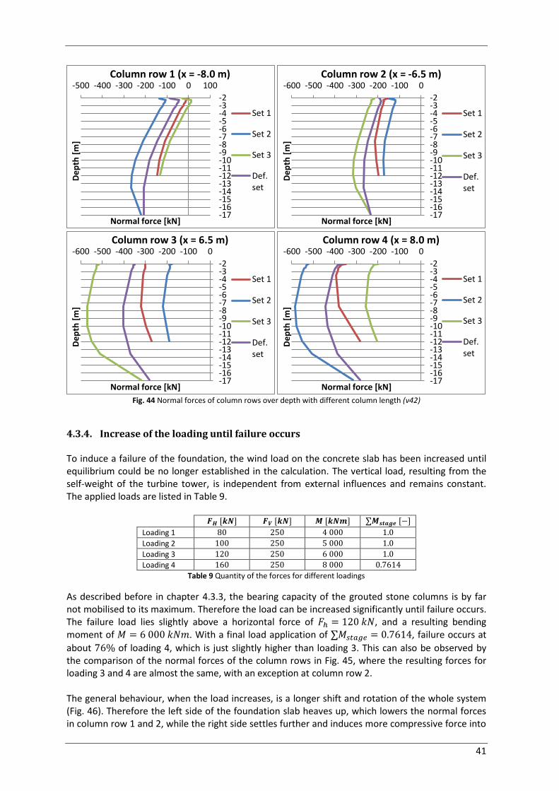
41

Fig. 44 Normal forces of column rows over depth with different column length (v42)

4.3.4. Increase of the loading until failure occurs To induce a failure of the foundation, the wind load on the concrete slab has been increased until equilibrium could be no longer established in the calculation. The vertical load, resulting from the self-weight of the turbine tower, is independent from external influences and remains constant. The applied loads are listed in Table 9.

Loading 1

Loading 2

Loading 3

Loading 4

Table 9 Quantity of the forces for different loadings

As described before in chapter 4.3.3, the bearing capacity of the grouted stone columns is by far not mobilised to its maximum. Therefore the load can be increased significantly until failure occurs. The failure load lies slightly above a horizontal force of , and a resulting bending moment of . With a final load application of , failure occurs at

about of loading 4, which is just slightly higher than loading 3. This can also be observed by the comparison of the normal forces of the column rows in Fig. 45, where the resulting forces for loading 3 and 4 are almost the same, with an exception at column row 2. The general behaviour, when the load increases, is a longer shift and rotation of the whole system (Fig. 46). Therefore the left side of the foundation slab heaves up, which lowers the normal forces in column row 1 and 2, while the right side settles further and induces more compressive force into

-17-16-15-14-13-12-11-10-9-8-7-6-5-4-3-2

-500 -400 -300 -200 -100 0 100D

ep

th [

m]

Normal force [kN]


Set 1

Set 2

Set 3

Def.set

-17-16-15-14-13-12-11-10-9-8-7-6-5-4-3-2

-600 -500 -400 -300 -200 -100 0

De

pth

[m

]

Normal force [kN]


Set 1

Set 2

Set 3

Def.set

-17-16-15-14-13-12-11-10-9-8-7-6-5-4-3-2

-600 -500 -400 -300 -200 -100 0

De

pth

[m

]

Normal force [kN]


Set 1

Set 2

Set 3

Def.set

-17-16-15-14-13-12-11-10-9-8-7-6-5-4-3-2

-600 -500 -400 -300 -200 -100 0

De

pth

[m

]

Normal force [kN]


Set 1

Set 2

Set 3

Def.set

42

column row 3 and 4. With the longer displacements of the foundation, also the bending of the columns increases, wherefore tensile forces are induced into the upper part of column row 1. The cause of these tensile forces is further investigated and discussed with the 3D model in chapter 5.1, in this case however they are not the reason for failure. Soil collapse however is then initiated by an opening gap beneath the left side of the foundation slab, due to elevation (Fig. 47), and does not take place at the column rows.

Fig. 45 Normal forces of column rows over depth with different moment loadings (v30.3.2)

Fig. 46 Total displacements due to a loading of and (v30.3.2)

-3.5-3.4-3.3-3.2-3.1-3-2.9-2.8-2.7-2.6-2.5-2.4-2.3-2.2-2.1-2

-500 -400 -300 -200 -100 0 100

De

pth

[m

]

Normal force [kN]


4000

5000

6000

8000

-3.5-3.4-3.3-3.2-3.1-3-2.9-2.8-2.7-2.6-2.5-2.4-2.3-2.2-2.1-2

-600 -500 -400 -300 -200 -100 0

De

pth

[m

]

Normal force [kN]


4000

5000

6000

8000

-3.5-3.4-3.3-3.2-3.1-3-2.9-2.8-2.7-2.6-2.5-2.4-2.3-2.2-2.1-2

-600 -500 -400 -300 -200 -100 0

De

pth

[m

]

Normal force [kN]


4000

5000

6000

8000

-3.5-3.4-3.3-3.2-3.1-3-2.9-2.8-2.7-2.6-2.5-2.4-2.3-2.2-2.1-2

-600 -500 -400 -300 -200 -100 0

De

pth

[m

]

Normal force [kN]


4000

5000

6000

8000

43

Fig. 47 Incremental deviatoric strain due to a loading of and (v30.3.2)

4.3.5. Modelling of foundation slab and load application In most of the previous calculations the foundation slab was modelled as linear elastic material. With this configuration a possible material failure at the anchorage point of the tower of the wind turbine is avoided. Besides that it disregards also possible failure of the concrete slab at the connection to the column rows due to the high bearing pressure. Because the slab is considered as concrete and will be reinforced, it is a lot more stable than the grouted stone columns, designed as unreinforced concrete. Therefore failure will not occur at the foundation slab, when even the columns do not collapse under the emerging bearing pressure, as can be seen in the calculations above. Nevertheless the effect of a slab with Mohr-Coulomb material model is investigated in this chapter.

Material model Linear elastic


Specific weight

Stiffness

Poisson's ratio

Cohesion

Friction angle

Dilatancy angle

Tensile strength

Interface strength




Specific weight

Stiffness

Poisson's ratio

Cohesion

Friction angle

Dilatancy angle

Tensile strength

Interface strength


Table 10 Input parameters for the foundation slab in LE and MC material model

Fig. 48 Mohr-Coulomb failure line for concrete

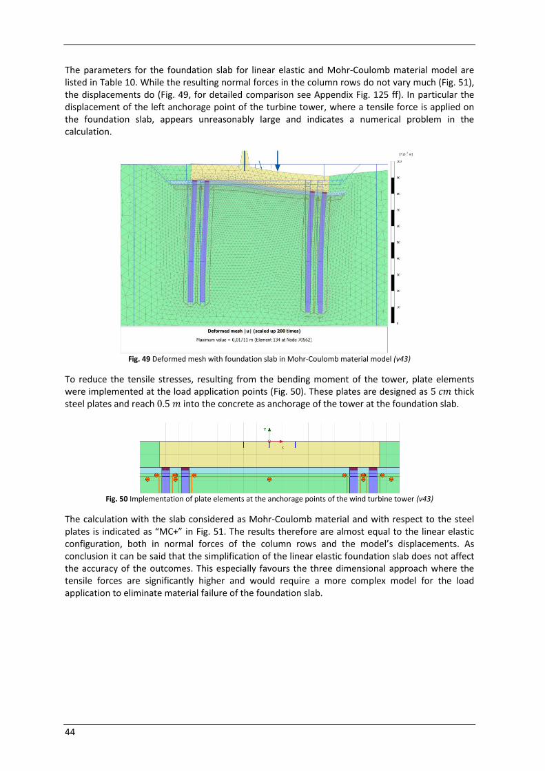
44

The parameters for the foundation slab for linear elastic and Mohr-Coulomb material model are listed in Table 10. While the resulting normal forces in the column rows do not vary much (Fig. 51), the displacements do (Fig. 49, for detailed comparison see Appendix Fig. 125 ff). In particular the displacement of the left anchorage point of the turbine tower, where a tensile force is applied on the foundation slab, appears unreasonably large and indicates a numerical problem in the calculation.

Fig. 49 Deformed mesh with foundation slab in Mohr-Coulomb material model (v43)

To reduce the tensile stresses, resulting from the bending moment of the tower, plate elements were implemented at the load application points (Fig. 50). These plates are designed as thick steel plates and reach into the concrete as anchorage of the tower at the foundation slab.

Fig. 50 Implementation of plate elements at the anchorage points of the wind turbine tower (v43)

The calculation with the slab considered as Mohr-Coulomb material and with respect to the steel plates is indicated as “MC+” in Fig. 51. The results therefore are almost equal to the linear elastic configuration, both in normal forces of the column rows and the model’s displacements. As conclusion it can be said that the simplification of the linear elastic foundation slab does not affect the accuracy of the outcomes. This especially favours the three dimensional approach where the tensile forces are significantly higher and would require a more complex model for the load application to eliminate material failure of the foundation slab.

45

Fig. 51 Normal forces of column rows over depth with different material models for the foundation slab and loading

plates (v43)

4.3.6. Comparison of stress integration, the structural forces in volumes-tool and beam

elements As a preliminary study for the calculations in 3D and additional to the investigation in chapter 2 plate elements have been placed within the column rows (Fig. 52) to enable another method to evaluate the normal forces in the columns, i.e. the axial forces of a soil cluster. In the previous calculations the normal forces of the column rows have been determined by integrating the normal stresses of horizontal cross sections, in different depths, over the width of the columns. For 2D calculations Plaxis offers the tool “Structural forces in volumes” to readout the normal forces, the shear forces and the bending moment along a linear line within a soil cluster. Because the tool also integrates the resulting stresses from the stress points over the width of the cluster along the drawn cross section line [5], the outcomes of the manual integration and the tool are the same (Fig. 53). Although the manual stress integration implies more effort, it was executed because it allows the interpolation of the normal force at any given cross section, whereas the tool provides the resulting forces only at certain depths near the stress points of the soil elements. Because no such tool is available in Plaxis for 3D calculations, and the stress integration over a two-dimensional cross section implies even more effort (see chapter A.1 in the Appendix), the main method to determine the normal force in a soil cluster is to implement a beam element, comparable with a plate element in 2D, at the centre of the particular cluster. Because the plate respectively beam elements are modelled as linear elastic material, this practice is only valid for a linear stress distribution over the cross section, independently of 2D or 3D.

-17-16-15-14-13-12-11-10-9-8-7-6-5-4-3-2

-800 -600 -400 -200 0D

ep

th [

m]

Normal force [kN]


LE

MC

MC+

-17-16-15-14-13-12-11-10-9-8-7-6-5-4-3-2

-800 -600 -400 -200 0

De

pth

[m

]

Normal force [kN]


LE

MC

MC+

-17-16-15-14-13-12-11-10-9-8-7-6-5-4-3-2

-800 -600 -400 -200 0

De

pth

[m

]

Normal force [kN]


LE

MC

MC+

-17-16-15-14-13-12-11-10-9-8-7-6-5-4-3-2

-800 -600 -400 -200 0

De

pth

[m

]

Normal force [kN]


LE

MC

MC+

46

Fig. 52 Plate elements within the column rows (v50)

Fig. 53 Normal forces of column rows over depth in default settings with different investigation methods: (1) plate

elements, (2) structural forces in volumes, (3) stress integration over cross section (v50)

To further analyse the accuracy of the different ways of evaluating axial forces, the resulting axial forces of the plate elements in the 2D model are compared to the outcomes of the stress integration in Fig. 53. The predicted axial forces in the column rows by the plate elements underestimate the actual normal forces significantly at the lower parts of the columns and show unrealistic peaks at the connection of the columns to the foundation slab. When the deviation at

-17-16-15-14-13-12-11-10-9-8-7-6-5-4-3-2

-400 -300 -200 -100 0 100

De

pth

[m

]

Normal force [kN]

Column 1 (x = -8.0 m)

(1)

(2)

(3)

-17-16-15-14-13-12-11-10-9-8-7-6-5-4-3-2

-500 -400 -300 -200 -100 0

De

pth

[m

]

Normal force [kN]

Column 2 (x = -6.5 m)

(1)

(2)

(3)

-17-16-15-14-13-12-11-10-9-8-7-6-5-4-3-2

-500 -400 -300 -200 -100 0

De

pth

[m

]

Normal force [kN]

Column 3 (x = 6.5 m)

(1)

(2)

(3)

-17-16-15-14-13-12-11-10-9-8-7-6-5-4-3-2

-500 -400 -300 -200 -100 0

De

pth

[m

]

Normal force [kN]

Column 4 (x = 8.0 m)

(1)

(2)

(3)

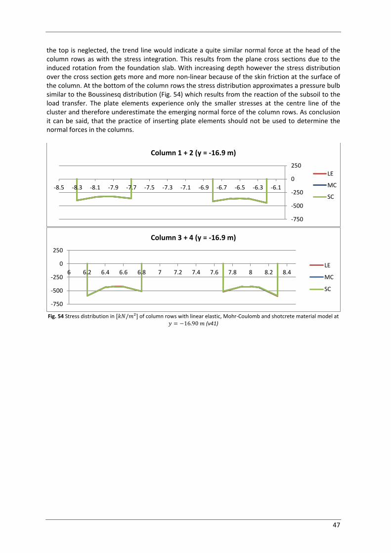
47

the top is neglected, the trend line would indicate a quite similar normal force at the head of the column rows as with the stress integration. This results from the plane cross sections due to the induced rotation from the foundation slab. With increasing depth however the stress distribution over the cross section gets more and more non-linear because of the skin friction at the surface of the column. At the bottom of the column rows the stress distribution approximates a pressure bulb similar to the Boussinesq distribution (Fig. 54) which results from the reaction of the subsoil to the load transfer. The plate elements experience only the smaller stresses at the centre line of the cluster and therefore underestimate the emerging normal force of the column rows. As conclusion it can be said, that the practice of inserting plate elements should not be used to determine the normal forces in the columns.

Fig. 54 Stress distribution in of column rows with linear elastic, Mohr-Coulomb and shotcrete material model at

(v41)

-750

-500

-250

0

250

-8.5 -8.3 -8.1 -7.9 -7.7 -7.5 -7.3 -7.1 -6.9 -6.7 -6.5 -6.3 -6.1

Column 1 + 2 (y = -16.9 m)

LE

MC

SC

-750

-500

-250

0

250

6 6.2 6.4 6.6 6.8 7 7.2 7.4 7.6 7.8 8 8.2 8.4

Column 3 + 4 (y = -16.9 m)

LE

MC

SC

48

5. Calculations in 3D A list of the performed analyses and their basic properties of the three dimensional model is given in Table 11. The calculations have been executed with Plaxis 3D from 2013 and are all based on the same generated model (Fig. 4). Version Subtitle Soil Columns Description

v01.30 Results without Beams

HSS SC connection of columns to foundation slab without tensile strength; no beams implemented

v01.40 Results with Beams

HSS SC connection of columns to foundation slab without tensile strength; beams implemented in columns

v01.41 Beams E25e6 HSS SC variation of beam stiffness to investigate influence on column mobilisation

v01.42 Max Load HSS SC double the load than default settings

v01.43 Piles -2.0 MIP HSS SC column heads at , connected to foundation slab; stabilized soil consists of MIP-layer

v01.44.1 Piles -2.5 Gravel HSS SC column heads at ; stabilized soil consists of gravel layer

v01.44.2 Piles -2.5 MIP HSS SC column heads at ; stabilized soil consists of MIP layer

v01.45 HSS SC

v01.46 HSS SC

v01.47 Tension softening

HSS SC connection of columns to foundation slab with respect to tensile strength

v01.48 Beams -2.2 HSS SC variation of beam application to investigate influence on column mobilisation

v01.49 m=0 HSS SC subsoil properties with power to neglect stress depending stiffness

v01.50 HS m=1 HS SC subsoil in Hardening Soil material model to neglect small strain stiffness

v01.51 without piles HSS SC calculation without columns to investigate model behaviour

v01.52 Piles without weight

HSS SC columns without self- weight to analyse influence on column mobilisation

v01.53 Piles without skin friction

HSS SC columns without skin friction to analyse influence on column mobilisation

Table 11 Calculations in 3D for chapter 5

As mentioned before the subsoil in the 3D model consists of three different clay layers with their properties related to the geotechnical study of the expansion of Corbu 2 project [3]. Similar to the investigations in 2D the layers were considered with the Hardening Soil small model and under drained conditions with no ground water table present. The input parameters are given in Table 12. The properties for the remaining materials are equal to those used in the 2D calculations. Therefore the foundation slab is considered as a linear elastic concrete material (Table 10) and the stabilized soil mainly consists of a gravel layer (Table 8). The grouted stone columns are again modelled with the shotcrete material model (Table 2) and the top layer is considered without any tensile strength to neglect a tensile bonding between the columns and the foundation slab. The materials and the colours used for representing them are shown in Table 13. Again only the settlements due to the external load on the foundation slab are shown in the following figures. To simplify the generated mesh and to reduce the required calculation time, only half of the system was used due to its symmetry. Therefore the loading from the turbine tower were applied as point loads and no load out of the symmetrical plane or torsional moment was considered, as mentioned in chapter 1.3.

49

Soil layer Clay 1 Clay 2 Clay 3 Material model HS small HS small HS small Drainage type drained drained drained Top level

Bottom level

Thickness Specific weight

Stiffness

Power

Poisson's ratio

Reference pressure

Earth pressure coeff. in normal consolidation

Cohesion

Friction angle

Dilatancy angle

Shear strain

Shear modulus

Permeability

Interface strength

Earth pressure coeff. for initial stress state

Table 12 Input parameters for subsoil in HSS-model for 3D calculations

Cluster/Element Material description Model Colour

Subsoil Clay 1 HSS

Clay 2 HSS

Clay 3 HSS

Foundation slab Concrete LE/MC

Grouted stone columns Concrete LE/MC/SC

Concrete with SC

Stabilized soil Gravel MC

Mixed-in-place (MIP) layer MC

Interface adopted from subsoil HSS

Beam elastic steel rod Elastic

Table 13 Colours of the soil clusters and structural elements in Plaxis 3D

The main aspect of the 3D calculations was once more the investigation of the normal force in the columns. If not mentioned differently, for determining them the method of the stress integration over the cross section with Surfer 12 was used, as described in chapter 2, due to the better accuracy compared to the use of dummy beam elements in the centre line of the column cluster. Although the columns highest loaded are column numbers 1.1 and 6.1, due to the longest distance from the load application at the centre of the foundation slab (Fig. 55), column number 1.2 and 6.2 were examined in detail. The reason for this is to overcome possible inaccuracies due to poor mesh quality over the boundary of the model. As shown in Fig. 56 for one loading case, the differences between those columns are negligible.

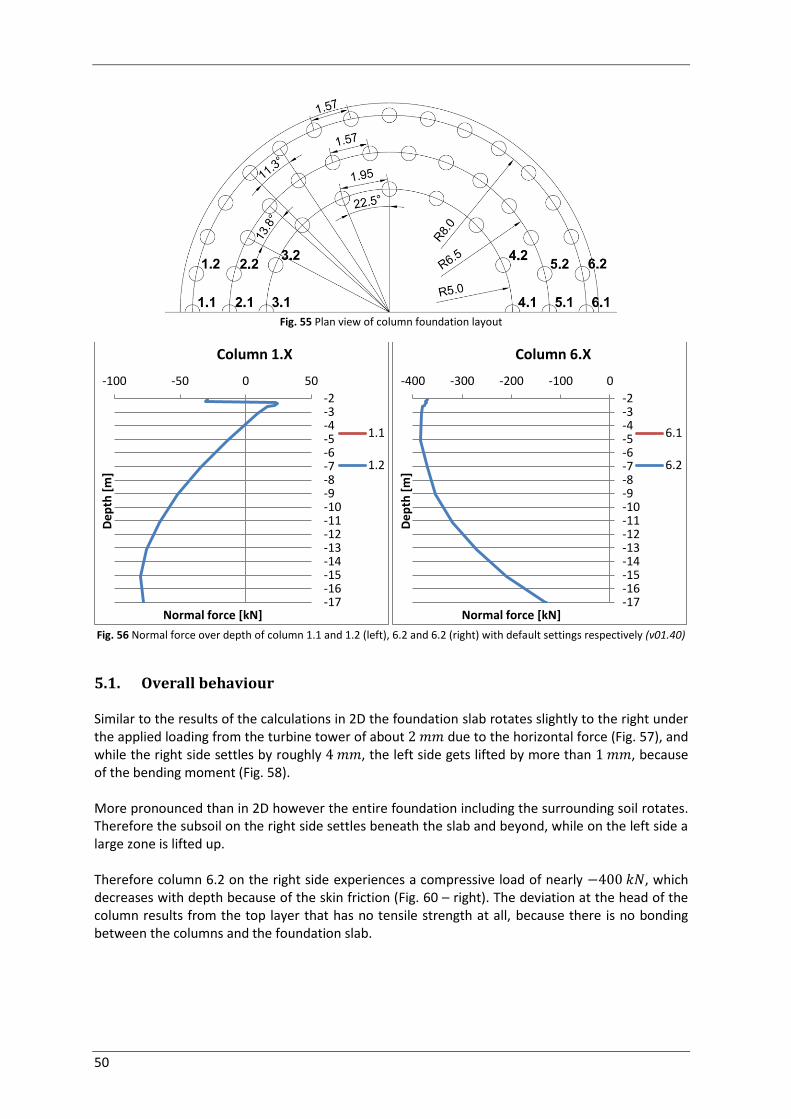
50

Fig. 55 Plan view of column foundation layout

Fig. 56 Normal force over depth of column 1.1 and 1.2 (left), 6.2 and 6.2 (right) with default settings respectively (v01.40)

5.1. Overall behaviour Similar to the results of the calculations in 2D the foundation slab rotates slightly to the right under the applied loading from the turbine tower of about due to the horizontal force (Fig. 57), and while the right side settles by roughly , the left side gets lifted by more than , because of the bending moment (Fig. 58). More pronounced than in 2D however the entire foundation including the surrounding soil rotates. Therefore the subsoil on the right side settles beneath the slab and beyond, while on the left side a large zone is lifted up. Therefore column 6.2 on the right side experiences a compressive load of nearly , which decreases with depth because of the skin friction (Fig. 60 – right). The deviation at the head of the column results from the top layer that has no tensile strength at all, because there is no bonding between the columns and the foundation slab.

-17-16-15-14-13-12-11-10-9-8-7-6-5-4-3-2

-100 -50 0 50

De

pth

[m

]

Normal force [kN]

Column 1.X

1.1

1.2

-17-16-15-14-13-12-11-10-9-8-7-6-5-4-3-2

-400 -300 -200 -100 0

De

pth

[m

]

Normal force [kN]

Column 6.X

6.1

6.2

51

Fig. 57 Total displacements with default settings (v01.40)

Fig. 58 Total displacements with default settings (v01.40)

On the left side however, as a result of the lifting of the foundation slab, also the stabilized soil layer and the clayey subsoil get lifted by almost the same amount as part of the slab (Fig. 59). Thus column 1.2 experiences bending in the upper part, which induces a tensile force into the column (Fig. 60 – left). This tensile force obviously disappears above in the top layer of the column, where the tensile strength is assumed to be zero.

52

Fig. 59 Total displacements of foundation slab with default settings (v01.40)

With depth however, the tensile force in column 1.2 reduces rather quickly, due to the effect of negative skin friction. Below a depth of about the normal force is compressive and increases further with depth. Although the entire column gets lifted, it reaches its maximum compressive normal force almost at the bottom of the column. The accuracy of the calculated normal force at the base can be reviewed by investigating the distribution of the axial stresses along the soil cluster and the interface element underneath the column (Fig. 61). The stress distribution over the interface element shows a pressure bulb, similar to the Boussinesq distribution, due to the reaction of the subsoil. With an average value of roughly , the resulting compressive force at the interface element calculates to about , which matches the determined value from the column reasonably well.

Fig. 60 Normal force of columns over depth with default settings (v01.40)

-17-16-15-14-13-12-11-10-9-8-7-6-5-4-3-2

-100 -75 -50 -25 0 25 50

De

pth

[m

]

Normal force [kN]

Column 1.2

-17-16-15-14-13-12-11-10-9-8-7-6-5-4-3-2

-400 -300 -200 -100 0

De

pth

[m

]

Normal force [kN]

Column 6.2

53

Fig. 61 Left: Cartesian effective stresses of column 1.2; right: effective normal stresses of bottom interface of

column 1.2 (v01.40)

The compressive normal force at the base of column 1.2 results from the initial loading of both, the self-weight of the column and the foundation slab (see chapter 5.3). While the column is loaded by compression during the construction process, the lift of the slab, due to the bending moment from the turbine tower, unloads the columns on the left side. Furthermore, because of the shift of the foundation slab, the columns experiences bending at the upper part, which induces the tensile forces and therefore lowers the compression, also in the lower part. As a result the maximum compressive force emerges at a depth of about (Fig. 60). Whereas the self-weight of the column generates only a small amount of the compressive force, most of it is due to the foundation slab. This can be reviewed by comparing the emerging normal forces of column 1.2 and 6.2 with different settings concerning the columns (Fig. 62). By neglecting only the self-weight of the columns (blue line), the compressive normal force of all columns is slightly smaller than with the default settings (red line), but the general force distribution is quite similar. In an additional analysis also the skin friction between the columns and the surrounding clay was set to a minimum by decreasing the interface strength to and . The skin friction in the stabilized soil layer at the top of the columns however was considered as in the default settings in the third approach (green line), but also reduced in the fourth (purple line). While the normal force at the top of column 1.2 is rather similar as before in the default settings, it reduces much slower with depth due to the almost neglected skin friction in (3) and (4). Still the normal force converts into a compressive force at a depth of about , respectively and reaches its maximum value at the bottom of the column. Because of the small remaining skin friction with an average of roughly , the total amount of axial force, transferred into the surrounding soil over the column’s surface area of , calculates to approximately .

54

This matches the difference of the normal force between the top and the base of both columns and explains the remaining compressive force in column 1.2. The little deviation between (3) and (4) results from the remaining skin friction in the stabilized soil layer in approach (3), which enables the transfer of a small amount of normal force already into the surrounding gravel at the top of the column. Column 6.2 however experiences a much lower compressive force at the top, due to the lower bearing capacity in (3) and (4), than the default settings (1). With a low skin friction the resistance against settlements relies almost completely on the contact pressure at the base. Therefore the displacements are much larger and more load is transferred by the contact pressure of the foundation slab. With depth the normal force slightly reduces, due to the little remaining skin friction, but does not decrease to the same value as in the default settings.

Fig. 62 Normal force of columns over depth with different settings: (1) columns with self-weight and skin friction, (2)

columns without self-weight but with skin friction, (3) columns without self-weight and no skin friction below , (4) columns without self-weight and no skin friction along entire column (v01.31; v01.32; v01.40; v01.52)

Fig. 63 Horizontal stress ( ) and shear stress over depth with original skin friction ( and reduced skin friction ( )

(v01.31; v01.32; v01.40)

-17-16-15-14-13-12-11-10-9-8-7-6-5-4-3-2

-100 -75 -50 -25 0 25 50

De

pth

[m

]

Normal force [kN]

Column 1.2

(1)

(2)

(3)

(4)

-17-16-15-14-13-12-11-10-9-8-7-6-5-4-3-2

-400 -300 -200 -100 0

De

pth

[m

]

Normal force [kN]

Column 6.2

(1)

(2)

(3)

(4)

-17-16-15-14-13-12-11-10-9-8-7-6-5-4-3-2

-200 -150 -100 -50 0 50 100

De

pth

[m

]

Stresses [kN/m²]

Column 1.2

σ'_n

τ +

τ -

-17-16-15-14-13-12-11-10-9-8-7-6-5-4-3-2

-200 -150 -100 -50 0 50 100

De

pth

[m

]

Stresses [kN/m²]

Column 6.2

σ'_n

τ +

τ -

55

The stresses , perpendicular to the column axis, onto the surface are quite similar at both columns and differ only at the top due to the higher bearing pressure from the foundation slab at the right side (Fig. 63). The change at the depth of and the jump at result from a change of the surrounding soil, which provide different specific weights or friction angles respectively. The interface strength of both configurations was set to rigid, what means that the strength parameters were not reduced at the contact area between the grouted stone columns and the subsoil. Therefore the occurring shear stresses along the column’s surface are calculated either with the friction angle of the surrounding soil ( or with a reduced friction angle of ( ), as described above.

5.2. Influence of the beam element on the model behaviour As mentioned before the method of reading out the axial force of a volume column by implementing a beam element along the centre line of the column cluster partially delivers inaccurate values of the normal force. Although this has been reviewed in chapter 2, beam elements have been implemented in some of the executed calculations to simplify qualitative analyses of the model behaviour. Therefore it has to be investigated if the beam elements have an influence on the calculated settlements and the resulting normal forces or not.

Fig. 64 Normal force over depth, determined via stress integration (above) and via beam elements (below): (1) no beam

elements at all, (2) beam elements with , (3) beam elements with starting at (v01.30; v01.40; v01.41; v01.41.2; v01.48)

-17-16-15-14-13-12-11-10-9-8-7-6-5-4-3-2

-100 -50 0 50 100

De

pth

[m

]

Normal force [kN]

Column 1.2

(1)

(2)

-17-16-15-14-13-12-11-10-9-8-7-6-5-4-3-2

-500 -400 -300 -200 -100 0

De

pth

[m

]

Normal force [kN]

Column 6.2

(1)

(2)

-17-16-15-14-13-12-11-10-9-8-7-6-5-4-3-2

-100 -50 0 50 100

De

pth

[m

]

Normal force [kN]

Column 1.2

(2)

(3)

-17-16-15-14-13-12-11-10-9-8-7-6-5-4-3-2

-500 -400 -300 -200 -100 0

De

pth

[m

]

Normal force [kN]

Column 6.2

(2)

(3)

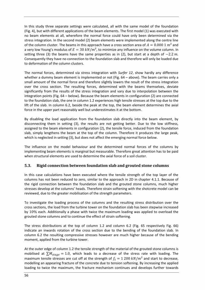
56

In this study three separate settings were calculated, all with the same model of the foundation (Fig. 4), but with different applications of the beam elements. The first model (1) was executed with no beam elements at all, wherefore the normal force could have only been determined via the stress integration. In the second model (2) beam elements were implemented along the centre line of the column cluster. The beams in this approach have a cross section area of and a very low Young’s modulus of , to minimize any influence on the volume column. In setting three (3) the beams have the same properties as in (2), but start at a depth of . Consequently they have no connection to the foundation slab and therefore will only be loaded due to deformation of the column clusters. The normal forces, determined via stress integration with Surfer 12, show hardly any difference whether a dummy beam element is implemented or not (Fig. 64 – above). The beam carries only a small amount of the normal force and therefore slightly lowers the result of the stress integration over the cross section. The resulting forces, determined with the beams themselves, deviate significantly from the results of the stress integration and vary due to interpolation between the integration points (Fig. 64 – below). Because the beam elements in configuration (2) are connected to the foundation slab, the one in column 1.2 experiences high tensile stresses at the top due to the lift of the slab. In column 6.2, beside the peak at the top, the beam element determines the axial force in the upper part reasonably well but underestimates it at the bottom. By disabling the load application from the foundation slab directly into the beam element, by disconnecting them in setting (3), the results are not getting better. Due to the low stiffness, assigned to the beam elements in configuration (2), the tensile force, induced from the foundation slab, simply lengthens the beam at the top of the column. Therefore it produces the large peak, which is neglected in setting (3), but does not affect the emerging normal force below. The influence on the model behaviour and the determined normal forces of the columns by implementing beam elements is marginal but measurable. Therefore great attention has to be paid when structural elements are used to determine the axial force of a soil cluster.

5.3. Rigid connection between foundation slab and grouted stone columns In this case calculations have been executed where the tensile strength of the top layer of the columns has not been reduced to zero, similar to the approach in 2D in chapter 4.1.1. Because of the rigid connection between the foundation slab and the grouted stone columns, much higher stresses develop at the columns’ heads. Therefore strain softening with the shotcrete model can be reviewed, due to the greater mobilisation of the strength parameters. To investigate the loading process of the columns and the resulting stress distribution over the cross sections, the load from the turbine tower on the foundation slab has been stepwise increased by each. Additionally a phase with twice the maximum loading was applied to overload the grouted stone columns and to continue the effect of strain softening. The stress distributions at the top of column 1.2 and column 6.2 (Fig. 65 respectively Fig. 66) indicate an inwards rotation of the cross section due to the bending of the foundation slab. In column 6.2 the resulting compressive stresses however are much higher because of the bending moment, applied from the turbine tower. At the outer edge of column 1.2 the tensile strength of the material of the grouted stone columns is mobilised at , which leads to a decrease of the stress rate with loading. The

maximum tensile stresses are cut off at the strength of and start to decrease, modelling an appearing fracture of the concrete due to tension softening. By increasing the applied loading to twice the maximum, the fracture mechanism continues and develops further towards

57

the centre of the cross section. The resulting stresses at the outer edge therefore reduce to zero, due to the opening crack, and the tensile stresses move inwards into the intact area of the column’s cross section.

Fig. 65 Stress distribution in of column 1.2 at with (above), (middle) and

twice the maximum load (below) (v01.47.2)

At column 6.2 however the tensile stresses are much smaller than in column 1.2 and disappear when the load is increased further, so no tension softening occurs. Furthermore, although the maximum compressive stresses calculated are higher, the compressive strength of is not reached. Therefore no strain softening takes place in this case and the cross section remains intact throughout the entire load application.

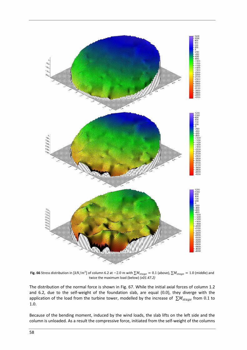
58

Fig. 66 Stress distribution in of column 6.2 at with (above), (middle) and

twice the maximum load (below) (v01.47.2)

The distribution of the normal force is shown in Fig. 67. While the initial axial forces of column 1.2 and 6.2, due to the self-weight of the foundation slab, are equal ( ), they diverge with the application of the load from the turbine tower, modelled by the increase of from to

. Because of the bending moment, induced by the wind loads, the slab lifts on the left side and the column is unloaded. As a result the compressive force, initiated from the self-weight of the columns

59

and the foundation slab, reduces. At full loading ( ) the axial force at the head of

column 1.2 turns into a tensile force, which is due to bending of the column, resulting from the shift and the rotation of the foundation slab under the external forces. The column is pulled out of the subsoil due to the horizontal shearing of the foundation slab along the column’s head. The tension is not directly transferred into the column by the lift of the slab, which can be observed by the comparison with the default setting (DS) where the tensile strength at the top layer of the column is reduced to zero and therefore no tensile stresses can be induced into the column. When the load is doubled ( ), this behaviour continues and almost the entire column is under tension. The curvature at the top of the graph results from the appearance of tension softening of the material, which reduces the tensile stresses, as described before. On the right side however, at column 6.2 compressive stresses increase, the higher the external loading. Because the cross section at the top of the column is almost completely under compression, the normal force results similar to the default settings, because no strain softening occurs. While the column is bending at the connection to the foundation slab as well, the compressive force is decreased by a small amount in the upper part. This effect is only observed at the top and disappears quickly over depth. Furthermore it reduces with an increase of the loading of the column. Even though the maximum normal force increases with the load application to almost three times the initial value, the pressure at the bottom of the column remains rather similar. As a consequence it means that most of the load is transferred into the surrounding soil via skin friction and only a relatively small amount via the base pressure. This indicates that the length of the grouted stone columns could be reduced without affecting the settlements of the foundation slab significantly. Furthermore the number of columns may be reduced, due to the fact that the emerging normal forces are far from reaching the bearing capacity of the columns of [2], and the resulting differential displacements of the foundation slab are significantly below the specified maximum of from the turbine producers.

Fig. 67 Normal force over depth with hinged connection and full loading at default settings (DS), rigid connection and

incremental loading with 0.0 to 1.0 and twice the maximum load (2.0) (v01.40; v01.47.2)

5.4. Increase of the loading Similar to the 2D model in chapter 4.3.4 the horizontal wind load on the turbine, and therefore the resulting bending moment on the foundation slab, have been increased to investigate the model behaviour in 3D until failure occurs. The applied loads are shown in Table 14.

-17-16-15-14-13-12-11-10-9-8-7-6-5-4-3-2

-200 -100 0 100 200

De

pth

[m

]

Normal force [kN]

Column 1.2

DS0.00.10.20.30.40.50.60.70.80.91.02.0

-17-16-15-14-13-12-11-10-9-8-7-6-5-4-3-2

-600 -500 -400 -300 -200 -100 0

De

pth

[m

]

Normal force [kN]

Column 6.2

DS0.00.10.20.30.40.50.60.70.80.91.02.0

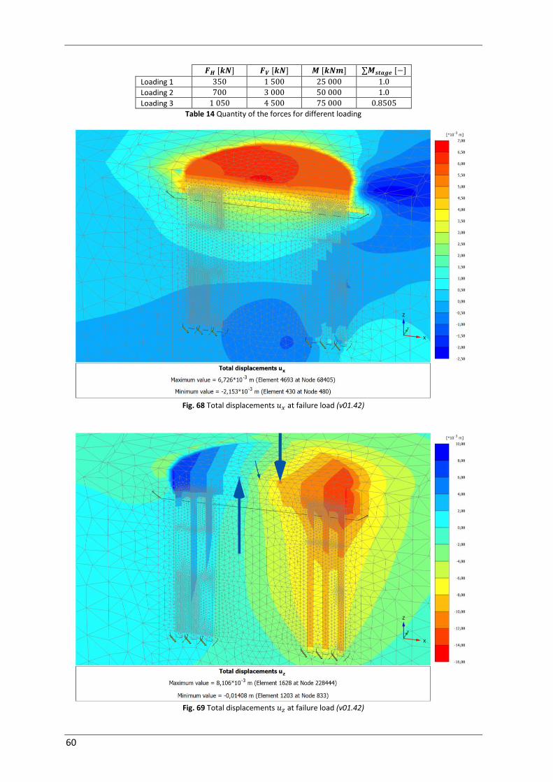
60

Loading 1

Loading 2

Loading 3

Table 14 Quantity of the forces for different loading

Fig. 68 Total displacements at failure load (v01.42)

Fig. 69 Total displacements at failure load (v01.42)

61

Due to the higher loading the horizontal shift and the rotation of the foundation slab, and therefore the displacement of the surrounding soil, increase (Fig. 68 and Fig. 69). As a result the bending of the grouted stone columns increases as well, which leads to higher tensile forces in column 1.2 with setting (2) (Fig. 70 – left). When the load is raised further in setting (3), the tensile stresses exceed the strength of the grouted stone columns and the columns on the left side crack completely (Fig. 71). This can be investigated by reviewing the utilisation of the tensile strength of the

material with the shotcrete model (Fig. 72; for a more detailed illustration see Appendix Fig. 128). In the upper part of column 1.2 the tensile strength is fully mobilised over the whole cross section, which indicates a tensile failure of the column.

Fig. 70 Normal force over depth with different loadings: (1) loading 1, (2) loading 2, (3) loading 3 (v01.42)

Fig. 71 Utilisation of tensile strength at failure load (v01.42)

-17-16-15-14-13-12-11-10-9-8-7-6-5-4-3-2

-100 -50 0 50 100 150 200 250

De

pth

[m

]

Normal force [kN]

Column 1.2

(1)

(2)

(3)

-17-16-15-14-13-12-11-10-9-8-7-6-5-4-3-2

-700 -600 -500 -400 -300 -200 -100 0

De

pth

[m

]

Normal force [kN]

Column 6.2

(1)

(2)

(3)

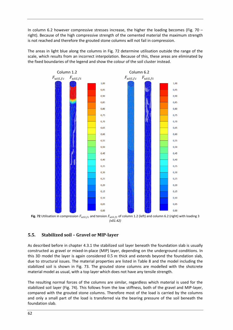
62

In column 6.2 however compressive stresses increase, the higher the loading becomes (Fig. 70 – right). Because of the high compressive strength of the cemented material the maximum strength is not reached and therefore the grouted stone columns will not fail in compression. The areas in light blue along the columns in Fig. 72 determine utilisation outside the range of the scale, which results from an incorrect interpolation. Because of this, these areas are eliminated by the fixed boundaries of the legend and show the colour of the soil cluster instead.

Column 1.2 Column 6.2

Fig. 72 Utilisation in compression and tension of column 1.2 (left) and column 6.2 (right) with loading 3

(v01.42)

5.5. Stabilized soil – Gravel or MIP-layer As described before in chapter 4.3.1 the stabilized soil layer beneath the foundation slab is usually constructed as gravel or mixed-in-place (MIP) layer, depending on the underground conditions. In this 3D model the layer is again considered thick and extends beyond the foundation slab, due to structural issues. The material properties are listed in Table 8 and the model including the stabilized soil is shown in Fig. 73. The grouted stone columns are modelled with the shotcrete material model as usual, with a top layer which does not have any tensile strength. The resulting normal forces of the columns are similar, regardless which material is used for the stabilized soil layer (Fig. 74). This follows from the low stiffness, both of the gravel and MIP-layer, compared with the grouted stone columns. Therefore most of the load is carried by the columns and only a small part of the load is transferred via the bearing pressure of the soil beneath the foundation slab.

63

Fig. 73 Model geometry with stabilized soil as MIP-layer (v01.43.2)

The deviation of the normal force in column 1.2 results from the higher skin friction of the MIP than the gravel layer. As described before the tensile force is partially transferred into the surrounding soil by the shear stresses along the column’s surface. Although the friction angle of the gravel is higher than the one of the MIP-layer, the skin friction is higher within the MIP-layer due to the high cohesion. It has to be questioned whether the assumption of a cohesion at the contact area between the grouted stone columns and the stabilized soil is valid, because both elements are constructed at different times. However the influence on the mobilisation of the columns is rather small.

Fig. 74 Normal force over depth with gravel and MIP-layer beneath foundation slab (v01.40; v01.43.2)

-17-16-15-14-13-12-11-10-9-8-7-6-5-4-3-2

-100 -50 0 50

De

pth

[m

]

Normal force [kN]

Column 1.2

Gravel

MIP

-17-16-15-14-13-12-11-10-9-8-7-6-5-4-3-2

-400 -300 -200 -100 0

De

pth

[m

]

Normal force [kN]

Column 6.2

Gravel

MIP

64

5.6. Connection of the column heads with the foundation slab Although the normal force of the columns on the right side is far from reaching the bearing capacity of [2], the peak stresses at the top of the columns are rather high due to the contact pressure induced by the foundation slab. Therefore, similar to chapter 4.3.2, an analysis was performed placing the head of the columns beneath the stabilized soil layer (Fig. 75).

Fig. 75 Model geometry with column heads beneath the stabilized soil layer at (v01.44.1)

By disconnecting the column heads from the foundation slab, the displacements of the upper part of the columns, because of the shift and the rotation of the slab, are slightly smaller. Therefore, in column 1.2, the tensile force, due to the bending of the column, disappears and the normal force at the top of the column converges to zero (Fig. 76). As a result the compressive force in the lower part is somewhat higher, but is similar to the reference calculation at the base of the column.

Fig. 76 Normal force over depth with different column heads: (1) column head at in gravel layer, (2) column head

at beneath gravel layer, (3) column head at beneath MIP-layer (v01.40; v01.44.1; v01.44.2)

-17-16-15-14-13-12-11-10-9-8-7-6-5-4-3-2

-100 -75 -50 -25 0 25 50

De

pth

[m

]

Normal force [kN]

Column 1.2

(1)

(2)

(3)

-17-16-15-14-13-12-11-10-9-8-7-6-5-4-3-2

-400 -300 -200 -100 0

De

pth

[m

]

Normal force [kN]

Column 6.2

(1)

(2)

(3)

65

At the right side however, in column 6.2, the normal force is smaller, because more of the load from the foundation slab is transferred into the subsoil. This is a consequence of the stabilized soil being softer than the grouted stone columns, which reduces the local pressure. As a result the maximum normal stresses at the top of the column are much smaller and more evenly distributed, although they have a shape similar to the Boussinesq distribution (Fig. 77). The deviation between configuration (2) and (3) in Fig. 76 follows from the different specific weight and Young’s modulus of the stabilized soil materials, whereas the MIP-layer is almost four times stiffer than the gravel layer. Therefore the normal force at the top of column 1.2 is slightly higher beneath the MIP-layer, due to the larger self-weight. At the right side however the load transfer from the foundation slab into column 6.2 is more efficient because of the stiffer MIP-layer.

Fig. 77 Stress distribution in over the cross section of column 6.2 at with the head beneath the

foundation slab (above) and at with the head beneath the gravel layer (below) (v01.40; v01.44.1)

5.7. Calculations with the HSS material model and the power set to In order to evaluate the influence of a stress dependent stiffness, calculations were executed assuming a constant stiffness for the subsoil. The clay layers were still modelled with the Hardening Soil small (HSS) material model, but the power was set to zero. The soil clusters now have a constant stiffness over depth.

66

Fig. 78 Total displacements with subsoil in HSS material model with the power (v01.49)

In this analysis the displacements are slightly higher (Fig. 78) but changes are not significant from a practical point of view in this case. With the HSS model the input values for the stiffness of the material, are valid for a specific reference stress. Therefore the Young’s moduli not only increase with depth, due to the higher overburden pressure, but also decrease towards the ground surface, when the effective stresses reduce. This means that by neglecting the effect of the stress dependent stiffness, the E modulus, now considered being constant, of the lower layers is smaller, but at the top layers is higher than before. As a result the pressure on the soil layer beneath the foundation slab is higher and more load is transferred into the clay, than in previous calculations (Fig. 80 and Fig. 81).

Fig. 79 Normal force over depth with subsoil in HSS material model with the power and (v01.40; v01.49)

-17-16-15-14-13-12-11-10-9-8-7-6-5-4-3-2

-100 -75 -50 -25 0 25 50

De

pth

[m

]

Normal force [kN]

Column 1.2

m = 1

m = 0

-17-16-15-14-13-12-11-10-9-8-7-6-5-4-3-2

-400 -300 -200 -100 0

De

pth

[m

]

Normal force [kN]

Column 6.2

m = 1

m = 0

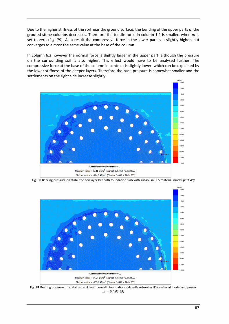
67

Due to the higher stiffness of the soil near the ground surface, the bending of the upper parts of the grouted stone columns decreases. Therefore the tensile force in column 1.2 is smaller, when is set to zero (Fig. 79). As a result the compressive force in the lower part is a slightly higher, but converges to almost the same value at the base of the column. In column 6.2 however the normal force is slightly larger in the upper part, although the pressure on the surrounding soil is also higher. This effect would have to be analysed further. The compressive force at the base of the column in contrast is slightly lower, which can be explained by the lower stiffness of the deeper layers. Therefore the base pressure is somewhat smaller and the settlements on the right side increase slightly.

Fig. 80 Bearing pressure on stabilized soil layer beneath foundation slab with subsoil in HSS material model (v01.40)

Fig. 81 Bearing pressure on stabilized soil layer beneath foundation slab with subsoil in HSS material model and power

(v01.49)

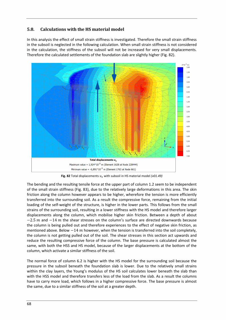
68

5.8. Calculations with the HS material model In this analysis the effect of small strain stiffness is investigated. Therefore the small strain stiffness in the subsoil is neglected in the following calculation. When small strain stiffness is not considered in the calculation, the stiffness of the subsoil will not be increased for very small displacements. Therefore the calculated settlements of the foundation slab are slightly higher (Fig. 82).

Fig. 82 Total displacements with subsoil in HS material model (v01.49)

The bending and the resulting tensile force at the upper part of column 1.2 seem to be independent of the small strain stiffness (Fig. 83), due to the relatively large deformations in this area. The skin friction along the column however appears to be higher, wherefore the tension is more efficiently transferred into the surrounding soil. As a result the compressive force, remaining from the initial loading of the self-weight of the structure, is higher in the lower parts. This follows from the small strains of the surrounding soil, resulting in a lower stiffness with the HS model and therefore larger displacements along the column, which mobilise higher skin friction. Between a depth of about and the shear stresses on the column’s surface are directed downwards because the column is being pulled out and therefore experiences to the effect of negative skin friction, as mentioned above. Below however, when the tension is transferred into the soil completely, the column is not getting pulled out of the soil. The shear stresses in this section act upwards and reduce the resulting compressive force of the column. The base pressure is calculated almost the same, with both the HSS and HS model, because of the larger displacements at the bottom of the column, which activate a similar stiffness of the soil. The normal force of column 6.2 is higher with the HS model for the surrounding soil because the pressure in the subsoil beneath the foundation slab is lower. Due to the relatively small strains within the clay layers, the Young’s modulus of the HS soil calculates lower beneath the slab than with the HSS model and therefore transfers less of the load from the slab. As a result the columns have to carry more load, which follows in a higher compressive force. The base pressure is almost the same, due to a similar stiffness of the soil at a greater depth.

69

This comparison shows the importance of choosing the appropriate material model for soil. By neglecting the small strain stiffness in the subsoil, not only the displacements will deviate by a considerable amount, but also the mobilisation of the grouted stone columns is effected noticeably.

Fig. 83 Normal force over depth with subsoil in HS material model (v01.50)

-17-16-15-14-13-12-11-10-9-8-7-6-5-4-3-2

-100 -75 -50 -25 0 25 50

De

pth

[m

]

Normal force [kN]

Column 1.2

HSS

HS

-17-16-15-14-13-12-11-10-9-8-7-6-5-4-3-2

-500 -400 -300 -200 -100 0

De

pth

[m

]

Normal force [kN]

Column 6.2

HSS

HS

70

6. Summary One of the main aspects in this thesis was to determine the normal force of a column modelled as soil cluster. Whereas the usual method for this task is placing a dummy structural element at the centre line of the cluster, this procedure delivers partially inaccurate results due to a non-linear stress distribution over the cross section. This follows from the reaction of the column with the surrounding subsoil and occurs also when linear elastic material is used. The deviation of the determined normal force can be reviewed by comparing it with the results of the integration of the axial stresses in the integration points over the cross section of the column (Fig. 84), as mentioned in the preliminary studies in chapter 2.1.

Fig. 84 Normal force over depth of single column modelled SC material model (Single pile study 2)

Another issue of the performed studies was to evaluate the shotcrete model [1] which was used to model the grouted stone columns of the foundation. Although it was originally developed for modelling shotcrete, the material model enabled the consideration of strain hardening and softening to approximate fracture propagation. Due to the rotation of the foundation slab tensile stresses are induced into the head of the columns which exceed the tensile strength and cause the material to crack. The distribution of the tensile stresses over the cross section can be observed in Fig. 85. While the external loading on the structure is increased stepwise, the tensile stresses reduce to zero, modelling a fracture of the material.

Fig. 85 Stress distribution in of cross section at with increase of , with shotcrete material model

(v30.3.1)

-10

-9

-8

-7

-6

-5

-4

-3

-2

-1

0

-300 -200 -100 0

De

pth

[m

]

Normal force [kN]

Single column - SC

Beam

Surfer

-4 000

-3 000

-2 000

-1 000

00

1 000

2 000

6 6.2 6.4 6.6 6.8 7 7.2 7.4 7.6 7.8 8 8.2 8.4

Column 3 + 4 (y = -2.0 m)

0.1

0.2

0.3

0.4

0.5

∑Mstage

71

The overall behaviour of the structure in the 3D calculations consists of a horizontal shift and a rotation due to wind loads. While all columns have the same normal force due to the self-weight of the structure at initiation of the external loading (Fig. 86 – 0.0), the rotation of the foundation slab, due to the bending moment induced by the turbine tower, unloads the columns on the left and loads the one on the right side. The horizontal displacement causes a shearing of the slab along the head of the columns, which pulls out the columns on the left and induces tensile forces. Over depth these tensile forces are transferred into the surrounding soil via skin friction and the compressive force in the lower part of column 1.2 still remains from the initial loading. The comparison with the default settings (DS) shows that tension can develop in the columns although there is no tensile strength considered at the connection between the foundation slab and the columns.

Fig. 86 Normal force over depth with hinged connection and full loading at default settings (DS), rigid connection and

incremental loading with 0.0 to 1.0 and twice the maximum load (2.0) (v01.40; v01.47.2)

-17-16-15-14-13-12-11-10-9-8-7-6-5-4-3-2

-200 -100 0 100 200

De

pth

[m

]

Normal force [kN]

Column 1.2

DS0.00.10.20.30.40.50.60.70.80.91.02.0

-17-16-15-14-13-12-11-10-9-8-7-6-5-4-3-2

-600 -500 -400 -300 -200 -100 0

De

pth

[m

]

Normal force [kN]

Column 6.2

DS0.00.10.20.30.40.50.60.70.80.91.02.0

72

References

[1] Schaedlich B., Schweiger H.F., Shotcrete model – Internal report: Implementation, validation and application of the shotcrete model. Computational Geotechnics Group, Graz University of Technology, 2014

[2] Aliciuc L., Petrescu E., Raport privind incercarile pe coloane de proba – Sistem mixt de fundare realizat din coloane de ballast stabilizat, vibrate. Geo 7 SRL, Keller Geotehnica SRL, 2012

[3] Stoica M., Studiu geotehnic pentru extindere parc eolian Corbu 2. S.C. GTF Prospect SRL, 2012

[4] Suzlon Energy A/S, Foundation Design Loads for S88 HH79.2 m. Suzlon Energy A/S – Denmark, 2006

[5] Plaxis, Plaxis 2D Anniversary Edition – Reference Manual. 2014 [6] Petternel P., Numerische Studien zum Tragverhalten von Pfählen und Pfahlgruppen in Plaxis

3D. Institut für Bodenmechanik und Grundbau, Technische Universität Graz, 2012 [7] Surfer, Surfer Demo Version 12 – Manual. Golden Software Inc., 2014

73

Appendix

A.1. Determining the normal force of a volume column with Surfer 12 [7] Surfer 12 from Golden Software is a mapping software to, amongst others, create three dimensional contour maps out of a list of points with their position coordinates and the appropriate altitude. In this work it is used to analyse the resulting normal force of a volume column from stress integration points. For this investigation a 3D model of a single column, loaded by a circular surface load of , was generated in Plaxis 3D. The column has a diameter of , a length of and is surrounded by clayey subsoil. To calculate the normal force, only the effective stresses in the axial direction, in this case , are of interest (Fig. 87).

Fig. 87 Cartesian stresses of volume column

The specific coordinates and the stress values of every stress point inside the soil cluster can be read out by viewing the table of soil elements (Fig. 88). If needed the table has to be sorted by the -coordinate to obtain the stress points properly arranged over depth. These stress values have then to be copied into either an Excel file or into a new worksheet in Surfer 12. Because of the easier editing of the table entries, the method with the Excel file was used in this thesis and will therefore be explained in this chapter.

74

Fig. 88 Table of soil elements with emerging stresses from Plaxis

With Surfer 12 it is not possible to determine the resulting normal force at every point over depth, but only for specified cross sections, selected by the user. To do so a small layer of the volume column, at the depth of interest, has to be extracted in the Excel table to consider all the stress points inside this layer, e.g. to determine the normal force at the head of the column, a layer of was considered at the top. Therefore only the entries between a depth of were left in the table while the others below were deleted. The stress values of this Excel file can now be processed with Surfer 12. At first a grid-file has to be generated by using the Grid – Data command. After selecting the particular Excel file and the right sheet, containing the stress values, the Grid Data windows opens (Fig. 89)

Fig. 89 Grid Data window in Surfer 12

Now the following adaptions have to be made. To read out the values of the stress points from the Excel file, the right columns have to be selected in the Data Columns. To allocate every stress value to its original position, the columns X and Y have to import the and -coordinates from the Excel sheet. The Z columns however should contain the stresses in the axial direction, therefore . This approach neglects the actual depth of each stress point, but smears the emerging stress values over the thickness of the extracted layer. The resulting deviation can be neglected because of the small thickness of the layer compared to the column length. The option Filter Data… was set to Average,

75

which means that if more than one stress value is located at the same position, the average value is taken into account. Furthermore the Gridding Method has been set to Natural Neighbor because this approach weights the calculated average of the axial stresses after the local data density of the available values and therefore delivers the actual mean value without considering the geometrical distribution over the cross section [7]. At last the directory and the name for the grid file was specified before it was created by clicking OK. The remaining options have been left at the default settings and were not investigated further. To illustrate the investigated stress distribution a three dimensional wireframe can be created from the grid file by using the Map – New – 3D wireframe… command and selecting the grid file created before. Therefore the Plot tab has to be active, to show the generated wireframe (Fig. 90). While this illustration can be used to visualize the stress distribution, it has to be considered that the grid file underestimates the dimensions of the cross section. This is due to the fact that all the stress points are located within the soil elements and therefore within the column cluster. As a result no stress values are available at the edge of the column and while Surfer interpolates values between the stress points, it is not aware of the actual dimension of the cross section and does not extrapolate the emerging stresses. This can also be seen in Fig. 90 whereas the maximum dimensions lie beneath the column’s radius of .

Fig. 90 Wireframe of stress distribution in over cross section with Surfer 12

Because of this reason the volume underneath the wireframe, which can be determined by the Grid – Volume… command, slightly underestimates the resulting normal force. The mean stress value of the grid file however, which is listed in the grid info report under Grid – Grid info…, can be multiplied with the actual area of the column’s cross section to calculate the axial force. Although the stress distribution in Fig. 90 seems quite irregular, which results from the smearing of the stress values over the layer and the irregular mesh of the soil cluster, the mean stress value is quite accurate and therefore predicted the normal force reasonably well. By following this method for several individual layers at different depths, the normal force can be determined for any cross section of the column and therefore be used to investigate the complete force distribution along the column. The described method was applied and reviewed on several geometries and settings with different material models like linear elastic and shotcrete model. It always delivered rather realistic values for the resulting normal force, even for nonlinear stress distributions over the cross section.

76

A.2. Soil parameters of Corbu 2 [3]

Soil layer

Name Description Level Thickness

Depth of investigation

[m] [m] [m] [m]

1 Clayey loess solid-stiff, brown-yellowish -0.50 -6.10 5.60 -4

2 Clay stiff, red-yellowish -6.10 -10.80 4.70 -6

3 Clay solid, greyish-green -10.80 -25.50 14.70 -12 / -18

Soil layer

Spec. weight Friction Cohesion Satur. Porosity Void ratio

Water content

Plastic limit

Flow limit

Plasticity index

Consistency index

d s cu ccu Sr n e w wP wL IP IC

[kN/m³] [kN/m³] [kN/m³] [°] [kPa] [-] [%] [-] [%] [%] [%] [%] [-]

1 16.0 13.7 26.7 31.2 7.1 0.45 48.59 0.95 16.20 16.84 35.09 18.25 1.03

2 19.2 15.7 27.0 18.4 62.0 0.83 41.98 0.72 22.42 15.63 60.70 45.07 0.84

3 20.4 17.1 27.2 19.6 78.6 0.94 37.80 0.61 20.21 21.76 61.74 39.98 1.04

Soil layer

Depth of investigation

Stiffness

Eoed,50 Eoed,100 Eoed,200 Eoed,300 Eoed,550 Eur,550-1

[m] [kPa] [kPa] [kPa] [kPa] [kPa] [kPa]

1 -4 1385 1792 2146 3515 5889 17710

2 -6 3731 5882 9132 12270 17361 26522

3.1 -12 6849 8850 14085 16667 22523 25126

3.2 -18 12245 12987 12658 13793 17621 21279

Table 15 Soil parameters, taken from the geotechnical study of Corbu 2 [3]

Soil layer

Stiffness Power Poisson's

Ratio Cohesion Friction

E50ref

Eoedref

Eurref

m ur c' '

[kN/m²] [kN/m²] [kN/m²] [-] [-] [kN/m²] [°]

1 14000 7000 42000 1 0.2 10 20

2 16000 8000 48000 1 0.2 20 25

3 20000 10000 60000 1 0.2 25 25

Table 16 Chosen soil parameters for the calculations in 3D

77

Soil layer 1

Pressure Strain Stiffness

'1 Eoed,secant Eoed,tangent

[kPa] [%] [kPa] [kPa]

25 1.70

-

1385

50 3.50 -

1524

100 6.78 1733

1942

200 11.93 2728

3515

300 14.78 4702

5889

550 19.02 7076

pref 100 [kPa] pref

εref 6.78 [%] εref (σ'1 = 100)

Eoed,ref 1700 [kPa] Eoed,ref (σ'1 = 100) -- tangent modulus

σ'1 550 [kPa] σ'1

ε 19.02 [%] εref (σ'1 = 550)

Eoed,100-550 3700 [kPa] Eoed = σ / -- secant modulus

Eoed,550 7100 [kPa] Eoed (σ'1 = 550) -- tangent modulus

m1 0.840 [-]

Eoed,1 7100 [kPa] Eoed = Eoed,ref * (σ'1 / pref)m_1

m2 0.948 [-]

Eoed,2 7100 [kPa] Eoed = Eoed,ref * [(cot ' * c' + σ'1) / (cot ' * c' + pref)]m_2

m 0.50 [-]

Eoed,1 4000 [kPa] Eoed = Eoed,ref * (σ'1 / pref)m

Eoed,2 3600 [kPa] Eoed = Eoed,ref * [(cot ' * c' + σ'1) / (cot ' * c' + pref)]m

m 0.75 [-]



m 1.00 [-]



Fig. 91 Investigation of and the power of soil layer 1

0.0

2.0

4.0

6.0

8.0

10.0

12.0

14.0

16.0

18.0

20.0

1 10 100 1000

ε [%

]

log σ'1 [kPa]

Layer 1

E_oed

0

100

200

300

400

500

600

0 2500 5000 7500 10000

σ'1

[kP

a]

E_oed,1 [kPa]

Layer 1

m = 0,50

m = 0,75

m = 0,84

m = 1,00

0

100

200

300

400

500

600

0 2500 5000 7500 10000

σ'1

[kP

a]

E_oed,2 [kPa]

Layer 1

m = 0,50

m = 0,75

m = 0,95

m = 1,00

78

Soil layer 2


σ'1 ε Eoed,secant Eoed,tangent


25 0.50

-

3731

50 1.17 -

5882

100 2.02 7507

9132

200 3.12 10701

12270

300 3.93 14816

17361

550 5.37 19907

pref 100 [kPa] pref

ε 2.02 [%] εref (σ'1 = 100)


σ'1 550 [kPa] σ'1

ε 5.37 [%] εref (σ'1 = 550)



m1 0.572 [-]


m2 0.686 [-]


m 0.50 [-]



m 0.75 [-]



m 1.00 [-]



Fig. 92 Investigation of and the power of soil layer 2

0.0

1.0

2.0

3.0

4.0

5.0

6.0

1 10 100 1000

ε [%

]

log σ'1 [kPa]

Layer 2

E_oed

0

100

200

300

400

500

600

0 15000 30000 45000

σ'1

[kP

a]

E_oed,1 [kPa]

Layer 2

m = 0,50

m = 0,57

m = 0,75

m = 1,00

0

100

200

300

400

500

600

0 15000 30000 45000

σ'1

[kP

a]

E_oed,2 [kPa]

Layer 2

m = 0,50

m = 0,69

m = 0,75

m = 1,00

79

Soil layer 3.1




25 0.37

-

6849

50 0.74 -

8850

100 1.30 11467

14085

200 2.01 15376

16667

300 2.61 19595

22523

550 3.72 25450

pref 100 [kPa] pref

ε 1.30 [%] εref (σ'1 = 100)


σ'1 550 [kPa] σ'1

ε 3.72 [%] εref (σ'1 = 550)



m1 0.468 [-]


m2 0.582 [-]


m 0.50 [-]



m 0.75 [-]



m 1.00 [-]



Fig. 93 Investigation of and the power of soil layer 3.1

0.0

0.5

1.0

1.5

2.0

2.5

3.0

3.5

4.0

1 10 100 1000

ε [%

]

log σ'1 [kPa]

Layer 3.1

E_oed

0

100

200

300

400

500

600

0 20000 40000 60000

σ'1

[kP

a]

E_oed,1 [kPa]

Layer 3.1

m = 0,47

m = 0,50

m = 0,75

m = 1,00

0

100

200

300

400

500

600

0 20000 40000 60000

σ'1

[kP

a]

E_oed,2 [kPa]

Layer 3.1

m = 0,50

m = 0,58

m = 0,75

m = 1,00

80

Soil layer 3.2




20 0.17

-

12245

50 0.41 -

12987

100 0.80 12823

12658

200 1.59 13226

13793

300 2.31 15707

17621

500 3.45 19535

pref 100 [kPa] pref

ε 0.80 [%] εref (σ'1 = 100)


σ'1 500 [kPa] σ'1

ε 3.45 [%] εref (σ'1 = 500)



m1 0.262 [-]


m2 0.328 [-]


m 0.50 [-]



m 0.75 [-]



m 1.00 [-]



Fig. 94 Investigation of and the power of soil layer 3.2

0.0

0.5

1.0

1.5

2.0

2.5

3.0

3.5

4.0

1 10 100 1000

ε [%

]

log σ'1 [kPa]

Layer 3.2

E_oed

0

100

200

300

400

500

600

0 20000 40000 60000

σ'1

[kP

a]

E_oed,1 [kPa]

Layer 3.2

m = 0,26

m = 0,50

m = 0,75

m = 1,00

0

100

200

300

400

500

600

0 20000 40000 60000

σ'1

[kP

a]

E_oed,2 [kPa]

Layer 3.2

m = 0,33

m = 0,50

m = 0,75

m = 1,00

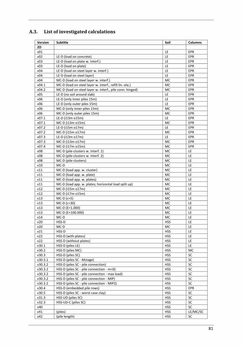
81

A.3. List of investigated calculations

Version Subtitle Soil Columns

2D

v01 LE EPR

v02 LE-D (load on concrete) LE EPR

v03 LE-D (load on plate w. interf.) LE EPR

v03 LE-D (load on plate) LE EPR

v04 LE-D (load on steel layer w. interf.) LE EPR

v04 LE-D (load on steel layer) LE EPR

v04 MC-D (load on steel layer w. interf.) MC EPR

v04.1 MC-D (load on steel layer w. interf., refill lin.-ela.) MC EPR

v04.2 MC-D (load on steel layer w. interf., pile conn. hinged) MC EPR

v05 LE-D (no soil around slab) LE EPR

v06 LE-D (only inner piles 15m) LE EPR

v06 LE-D (only outer piles 15m) LE EPR

v06 MC-D (only inner piles 15m) MC EPR

v06 MC-D (only outer piles 15m) MC EPR

v07.1 LE-D (i13m o15m) LE EPR

v07.1 MC-D (i13m o15m) MC EPR






v08 MC-D (pile-clusters w. Interf. 1) MC LE

v08 MC-D (pile-clusters w. Interf. 2) MC LE

v08 MC-D (pile-clusters) MC LE

v10 MC-D MC LE

v11 MC-D (load app. w. cluster) MC LE

v11 MC-D (load app. w. plate) MC LE

v11 MC-D (load app. w. plates) MC LE

v11 MC-D (load app. w. plates; horizontal load split up) MC LE

v12 MC-D (i15m o17m) MC LE

v12 MC-D (i17m o15m) MC LE

v13 MC-D (c=5) MC LE

v13 MC-D (c=30) MC LE

v13 MC-D (E=1.000) MC LE

v13 MC-D (E=100.000) MC LE

v14 MC-D MC LE

v20 HSS-D HSS LE

v20 MC-D MC LE

v21 HSS-D HSS LE

v22 HSS-D (with plates) HSS LE

v22 HSS-D (without plates) HSS LE

v30.1 HSS-D (piles LE) HSS LE

v30.2 HSS-D (piles MC) HSS MC

v30.3 HSS-D (piles SC) HSS SC

v30.3.1 HSS-D (piles SC - Mstage) HSS SC

v30.3.2 HSS-D (piles SC - pile connection) HSS SC

v30.3.2 HSS-D (piles SC - pile connection - m=0) HSS SC

v30.3.2 HSS-D (piles SC - pile connection - max load) HSS SC

v30.3.2 HSS-D (piles SC - pile connection - MIP) HSS SC

v30.3.2 HSS-D (piles SC - pile connection - MIP2) HSS SC

v30.4 HSS-D (embedded pile rows) HSS EPR

v30.5 HSS-D (piles SC - worst case clay) HSS SC

v31.3 HSS-UD (piles SC) HSS SC

v32.3 HSS-UD-C (piles SC) HSS SC

v40 HSS SC

v41 (piles) HSS LE/MC/SC

v42 (pile length) HSS SC

82

v43 (load application) HSS SC

v44 (Mstage) HSS SC

v44.2 (Mstage SC with ft) HSS SC

v45 (soil) LE/MC/HSS SC

v46 (undrained) HSS SC

v47 (MIP) HSS SC

v47.2 (MIP arc length contr. off) HSS SC

v47.3 (MIP ft=0) HSS SC

v48 (gravel) HSS SC

v49 (Fh160 M0) HSS SC

v49.2 (Fh160 M0 arc length. control off) HSS SC

v49.3 (Fh fail) HSS SC

v50 (beams) HSS SC

3D

v01.30 HSS SC

v01.30 Results without Beams HSS SC

v01.31 Piles without weight and skin friction HSS SC

v01.32 Piles without weight and skin friction HSS SC

v01.40 Results with Beams HSS SC

v01.41 Beams E25e6 HSS SC

v01.41.2 Beams E25e6 HSS SC

v01.42 Max Load HSS SC

v01.43.2 Piles -2.0 MIP HSS SC

v01.44.1 Piles -2.5 Gravel HSS SC

v01.44.2 Piles -2.5 MIP HSS SC

v01.45 Piles -2.5 MIP ft HSS SC

v01.46 Undrained HSS SC

v01.47 Tension softening HSS SC

v01.47.2 Mstage HSS SC

v01.48 Beams -2.2 HSS SC

v01.49 m=0 HSS SC

v01.49.2 HS m=0 HS SC

v01.50 HS m=1 HS SC

v01.50.2 HS m=1 Beams -2.2m HS SC

v01.51 without Piles HSS SC

v01.52 Piles without weight HSS SC

v01.53 Piles without skin friction HSS SC

- Double Pile Study HSS SC

- Single Pile Study HSS SC

- Single Pile Study 2 HSS LE/SC

Table 17 List of executed calculations with Plaxis

83

A.4. Further calculation results

Fig. 95 Deformed mesh with shotcrete model in default settings (v41)

Fig. 96 Incremental deviatoric strain with shotcrete model in default settings (v41)

84

Fig. 97 Principal effective stress with shotcrete model in default settings (v41)

Fig. 98 Principal effective stress with shotcrete model in default settings (v41)

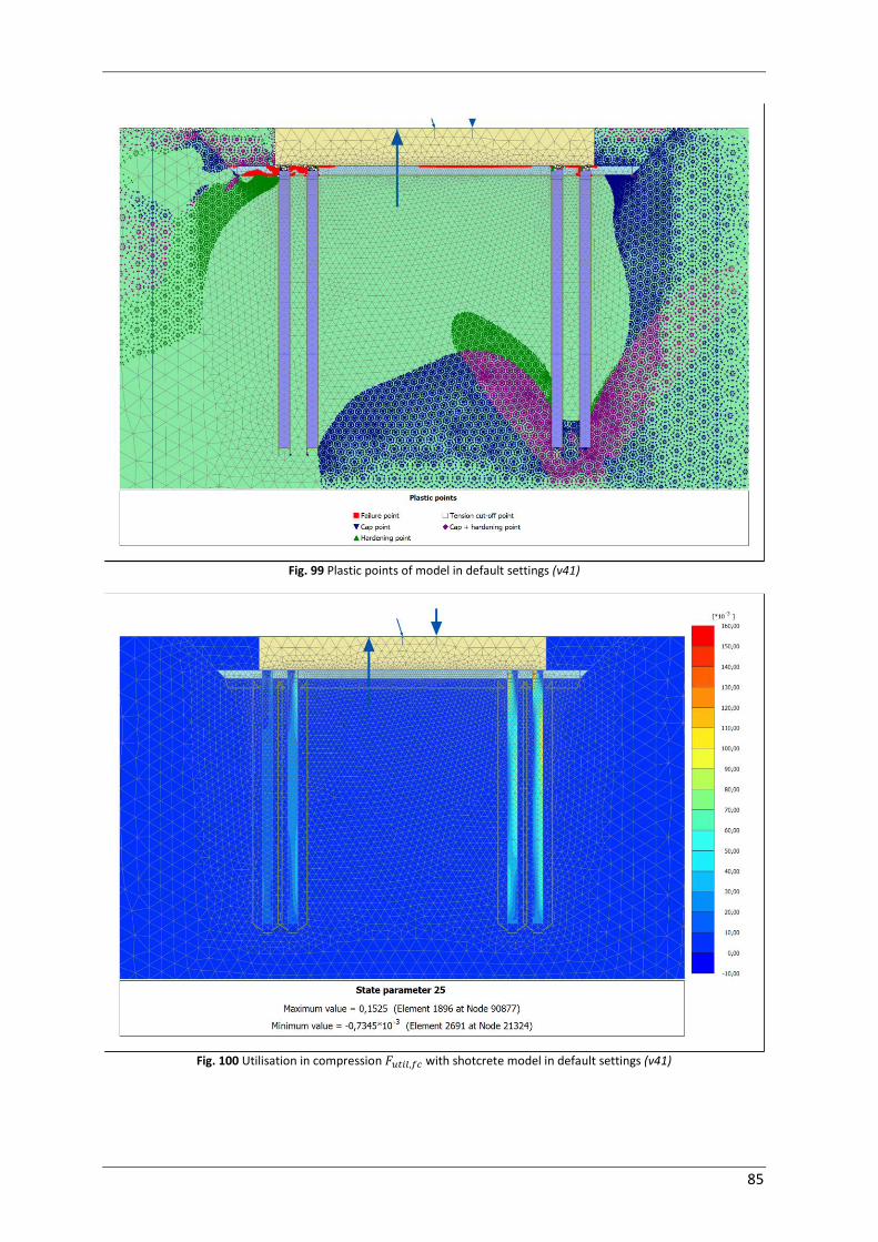
85

Fig. 99 Plastic points of model in default settings (v41)

Fig. 100 Utilisation in compression with shotcrete model in default settings (v41)

86

Fig. 101 Utilisation in tension with shotcrete model in default settings (v41)

Fig. 102 Relative shear stress with shotcrete model in default settings (v41)

87

Fig. 103 Stress distribution in of column rows with linear elastic, Mohr-Coulomb and shotcrete material model

at (v41)


at (v41)

-5000

-4000

-3000

-2000

-1000

0

1000

2000

-8.5 -8.3 -8.1 -7.9 -7.7 -7.5 -7.3 -7.1 -6.9 -6.7 -6.5 -6.3 -6.1

Column 1 + 2 (y = -2.05 m)

LE

MC

SC

-5000

-4000

-3000

-2000

-1000

0

1000

2000

6 6.2 6.4 6.6 6.8 7 7.2 7.4 7.6 7.8 8 8.2 8.4

Column 3 + 4 (y = -2.05 m)

LE

MC

SC

-5000

-4000

-3000

-2000

-1000

0

1000

2000

-8.5 -8.3 -8.1 -7.9 -7.7 -7.5 -7.3 -7.1 -6.9 -6.7 -6.5 -6.3 -6.1

Column 1 + 2 (y = -2.25 m)

LE

MC

SC

-5000

-4000

-3000

-2000

-1000

0

1000

2000

6 6.2 6.4 6.6 6.8 7 7.2 7.4 7.6 7.8 8 8.2 8.4

Column 3 + 4 (y = -2.25 m)

LE

MC

SC

88


at (v41)


at (v41)

-2000

-1000

0

1000

2000

-8.5 -8.3 -8.1 -7.9 -7.7 -7.5 -7.3 -7.1 -6.9 -6.7 -6.5 -6.3 -6.1

Column 1 + 2 (y = -7.50 m)

LE

MC

SC

-2000

-1000

0

1000

2000

6 6.2 6.4 6.6 6.8 7 7.2 7.4 7.6 7.8 8 8.2 8.4

Column 3 + 4 (y = -7.50 m)

LE

MC

SC

-2000

-1000

0

1000

2000

-8.5 -8.3 -8.1 -7.9 -7.7 -7.5 -7.3 -7.1 -6.9 -6.7 -6.5 -6.3 -6.1

Column 1 + 2 (y = -16.9 m)

LE

MC

SC

-2000

-1000

0

1000

2000

6 6.2 6.4 6.6 6.8 7 7.2 7.4 7.6 7.8 8 8.2 8.4

Column 3 + 4 (y = -16.9 m)

LE

MC

SC

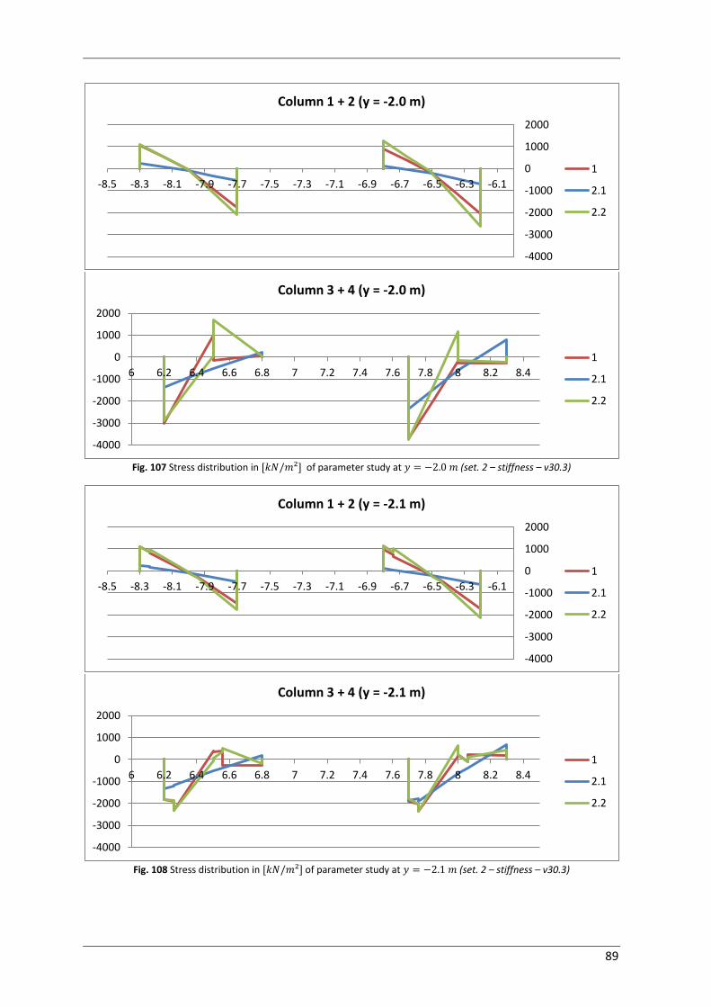
89



-4000

-3000

-2000

-1000

0

1000

2000

-8.5 -8.3 -8.1 -7.9 -7.7 -7.5 -7.3 -7.1 -6.9 -6.7 -6.5 -6.3 -6.1

Column 1 + 2 (y = -2.0 m)

1

2.1

2.2

-4000

-3000

-2000

-1000

0

1000

2000

6 6.2 6.4 6.6 6.8 7 7.2 7.4 7.6 7.8 8 8.2 8.4

Column 3 + 4 (y = -2.0 m)

1

2.1

2.2

-4000

-3000

-2000

-1000

0

1000

2000

-8.5 -8.3 -8.1 -7.9 -7.7 -7.5 -7.3 -7.1 -6.9 -6.7 -6.5 -6.3 -6.1

Column 1 + 2 (y = -2.1 m)

1

2.1

2.2

-4000

-3000

-2000

-1000

0

1000

2000

6 6.2 6.4 6.6 6.8 7 7.2 7.4 7.6 7.8 8 8.2 8.4

Column 3 + 4 (y = -2.1 m)

1

2.1

2.2

90



-4000

-3000

-2000

-1000

0

1000

2000

-8.5 -8.3 -8.1 -7.9 -7.7 -7.5 -7.3 -7.1 -6.9 -6.7 -6.5 -6.3 -6.1

Column 1 + 2 (y = -2.2 m)

1

2.1

2.2

-4000

-3000

-2000

-1000

0

1000

2000

6 6.2 6.4 6.6 6.8 7 7.2 7.4 7.6 7.8 8 8.2 8.4

Column 3 + 4 (y = -2.2 m)

1

2.1

2.2

-4000

-3000

-2000

-1000

0

1000

2000

-8.5 -8.3 -8.1 -7.9 -7.7 -7.5 -7.3 -7.1 -6.9 -6.7 -6.5 -6.3 -6.1

Column 1 + 2 (y = -2.4 m)

1

2.1

2.2

-4000

-3000

-2000

-1000

0

1000

2000

6 6.2 6.4 6.6 6.8 7 7.2 7.4 7.6 7.8 8 8.2 8.4

Column 3 + 4 (y = -2.4 m)

1

2.1

2.2

91



-4000

-3000

-2000

-1000

0

1000

2000

-8.5 -8.3 -8.1 -7.9 -7.7 -7.5 -7.3 -7.1 -6.9 -6.7 -6.5 -6.3 -6.1

Column 1 + 2 (y = -2.0 m)

1

3.1

3.2

3.3

-4000

-3000

-2000

-1000

0

1000

2000

6 6.2 6.4 6.6 6.8 7 7.2 7.4 7.6 7.8 8 8.2 8.4

Column 3 + 4 (y = -2.0 m)

1

3.1

3.2

3.3

-4000

-3000

-2000

-1000

0

1000

2000

-8.5 -8.3 -8.1 -7.9 -7.7 -7.5 -7.3 -7.1 -6.9 -6.7 -6.5 -6.3 -6.1

Column 1 + 2 (y = -2.1 m)

1

3.1

3.2

3.3

-4000

-3000

-2000

-1000

0

1000

2000

6 6.2 6.4 6.6 6.8 7 7.2 7.4 7.6 7.8 8 8.2 8.4

Column 3 + 4 (y = -2.1 m)

1

3.1

3.2

3.3

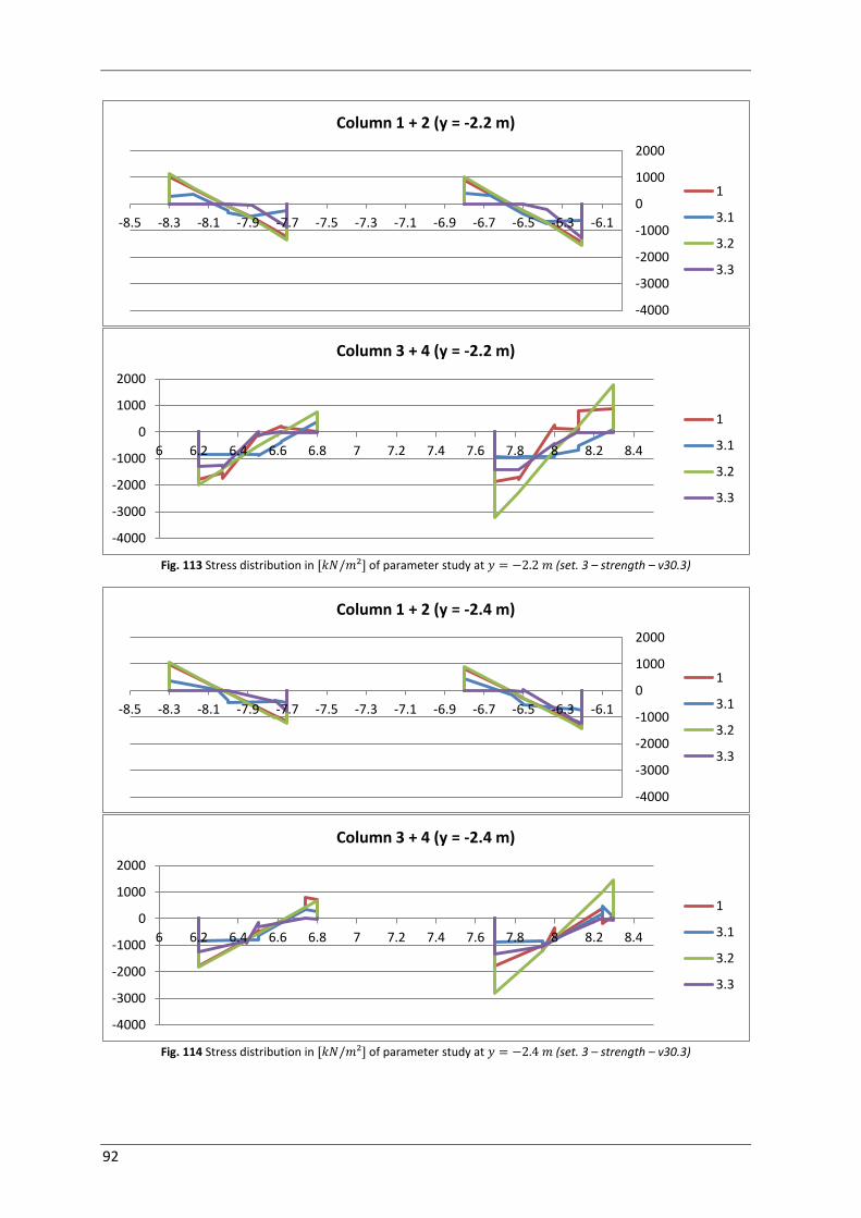
92



-4000

-3000

-2000

-1000

0

1000

2000

-8.5 -8.3 -8.1 -7.9 -7.7 -7.5 -7.3 -7.1 -6.9 -6.7 -6.5 -6.3 -6.1

Column 1 + 2 (y = -2.2 m)

1

3.1

3.2

3.3

-4000

-3000

-2000

-1000

0

1000

2000

6 6.2 6.4 6.6 6.8 7 7.2 7.4 7.6 7.8 8 8.2 8.4

Column 3 + 4 (y = -2.2 m)

1

3.1

3.2

3.3

-4000

-3000

-2000

-1000

0

1000

2000

-8.5 -8.3 -8.1 -7.9 -7.7 -7.5 -7.3 -7.1 -6.9 -6.7 -6.5 -6.3 -6.1

Column 1 + 2 (y = -2.4 m)

1

3.1

3.2

3.3

-4000

-3000

-2000

-1000

0

1000

2000

6 6.2 6.4 6.6 6.8 7 7.2 7.4 7.6 7.8 8 8.2 8.4

Column 3 + 4 (y = -2.4 m)

1

3.1

3.2

3.3

93



-4000

-3000

-2000

-1000

0

1000

2000

-8.5 -8.3 -8.1 -7.9 -7.7 -7.5 -7.3 -7.1 -6.9 -6.7 -6.5 -6.3 -6.1

Column 1 + 2 (y = -2.0 m)

1

4.1

4.2

-4000

-3000

-2000

-1000

0

1000

2000

6 6.2 6.4 6.6 6.8 7 7.2 7.4 7.6 7.8 8 8.2 8.4

Column 3 + 4 (y = -2.0 m)

1

4.1

4.2

-4000

-3000

-2000

-1000

0

1000

2000

-8.5 -8.3 -8.1 -7.9 -7.7 -7.5 -7.3 -7.1 -6.9 -6.7 -6.5 -6.3 -6.1

Column 1 + 2 (y = -2.1 m)

1

4.1

4.2

-4000

-3000

-2000

-1000

0

1000

2000

6 6.2 6.4 6.6 6.8 7 7.2 7.4 7.6 7.8 8 8.2 8.4

Column 3 + 4 (y = -2.1 m)

1

4.1

4.2

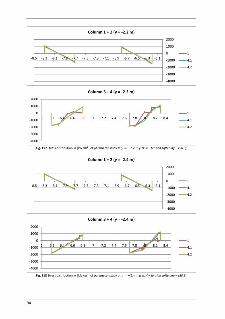
94



-4000

-3000

-2000

-1000

0

1000

2000

-8.5 -8.3 -8.1 -7.9 -7.7 -7.5 -7.3 -7.1 -6.9 -6.7 -6.5 -6.3 -6.1

Column 1 + 2 (y = -2.2 m)

1

4.1

4.2

-4000

-3000

-2000

-1000

0

1000

2000

6 6.2 6.4 6.6 6.8 7 7.2 7.4 7.6 7.8 8 8.2 8.4

Column 3 + 4 (y = -2.2 m)

1

4.1

4.2

-4000

-3000

-2000

-1000

0

1000

2000

-8.5 -8.3 -8.1 -7.9 -7.7 -7.5 -7.3 -7.1 -6.9 -6.7 -6.5 -6.3 -6.1

Column 1 + 2 (y = -2.4 m)

1

4.1

4.2

-4000

-3000

-2000

-1000

0

1000

2000

6 6.2 6.4 6.6 6.8 7 7.2 7.4 7.6 7.8 8 8.2 8.4

Column 3 + 4 (y = -2.4 m)

1

4.1

4.2

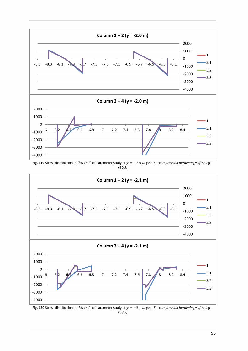
95


v30.3)


v30.3)

-4000

-3000

-2000

-1000

0

1000

2000

-8.5 -8.3 -8.1 -7.9 -7.7 -7.5 -7.3 -7.1 -6.9 -6.7 -6.5 -6.3 -6.1

Column 1 + 2 (y = -2.0 m)

1

5.1

5.2

5.3

-4000

-3000

-2000

-1000

0

1000

2000

6 6.2 6.4 6.6 6.8 7 7.2 7.4 7.6 7.8 8 8.2 8.4

Column 3 + 4 (y = -2.0 m)

1

5.1

5.2

5.3

-4000

-3000

-2000

-1000

0

1000

2000

-8.5 -8.3 -8.1 -7.9 -7.7 -7.5 -7.3 -7.1 -6.9 -6.7 -6.5 -6.3 -6.1

Column 1 + 2 (y = -2.1 m)

1

5.1

5.2

5.3

-4000

-3000

-2000

-1000

0

1000

2000

6 6.2 6.4 6.6 6.8 7 7.2 7.4 7.6 7.8 8 8.2 8.4

Column 3 + 4 (y = -2.1 m)

1

5.1

5.2

5.3

96


v30.3)


v30.3)

-4000

-3000

-2000

-1000

0

1000

2000

-8.5 -8.3 -8.1 -7.9 -7.7 -7.5 -7.3 -7.1 -6.9 -6.7 -6.5 -6.3 -6.1

Column 1 + 2 (y = -2.2 m)

1

5.1

5.2

5.3

-4000

-3000

-2000

-1000

0

1000

2000

6 6.2 6.4 6.6 6.8 7 7.2 7.4 7.6 7.8 8 8.2 8.4

Column 3 + 4 (y = -2.2 m)

1

5.1

5.2

5.3

-4000

-3000

-2000

-1000

0

1000

2000

-8.5 -8.3 -8.1 -7.9 -7.7 -7.5 -7.3 -7.1 -6.9 -6.7 -6.5 -6.3 -6.1

Column 1 + 2 (y = -2.4 m)

1

5.1

5.2

5.3

-4000

-3000

-2000

-1000

0

1000

2000

6 6.2 6.4 6.6 6.8 7 7.2 7.4 7.6 7.8 8 8.2 8.4

Column 3 + 4 (y = -2.4 m)

1

5.1

5.2

5.3

97

Fig. 123 Stress distribution in with a MIP-layer and different height of column heads at (v47.3)

Fig. 124 Stress distribution in with a MIP-layer and different height of column heads at (v47.3)

-2000

-1500

-1000

-500

0

500

1000

-8.5 -8.3 -8.1 -7.9 -7.7 -7.5 -7.3 -7.1 -6.9 -6.7 -6.5 -6.3 -6.1

Column 1 + 2 (y = -2.05 m)

-2.0 m

-2.5 m

-2000

-1500

-1000

-500

0

500

1000

6 6.2 6.4 6.6 6.8 7 7.2 7.4 7.6 7.8 8 8.2 8.4

Column 3 + 4 (y = -2.05 m)

-2.0 m

-2.5 m

-2000

-1500

-1000

-500

0

500

1000

-8.5 -8.3 -8.1 -7.9 -7.7 -7.5 -7.3 -7.1 -6.9 -6.7 -6.5 -6.3 -6.1

Column 1 + 2 (y = -2.55 m)

-2.0 m

-2.5 m

-2000

-1500

-1000

-500

0

500

1000

6 6.2 6.4 6.6 6.8 7 7.2 7.4 7.6 7.8 8 8.2 8.4

Column 3 + 4 (y = -2.55 m)

-2.0 m

-2.5 m

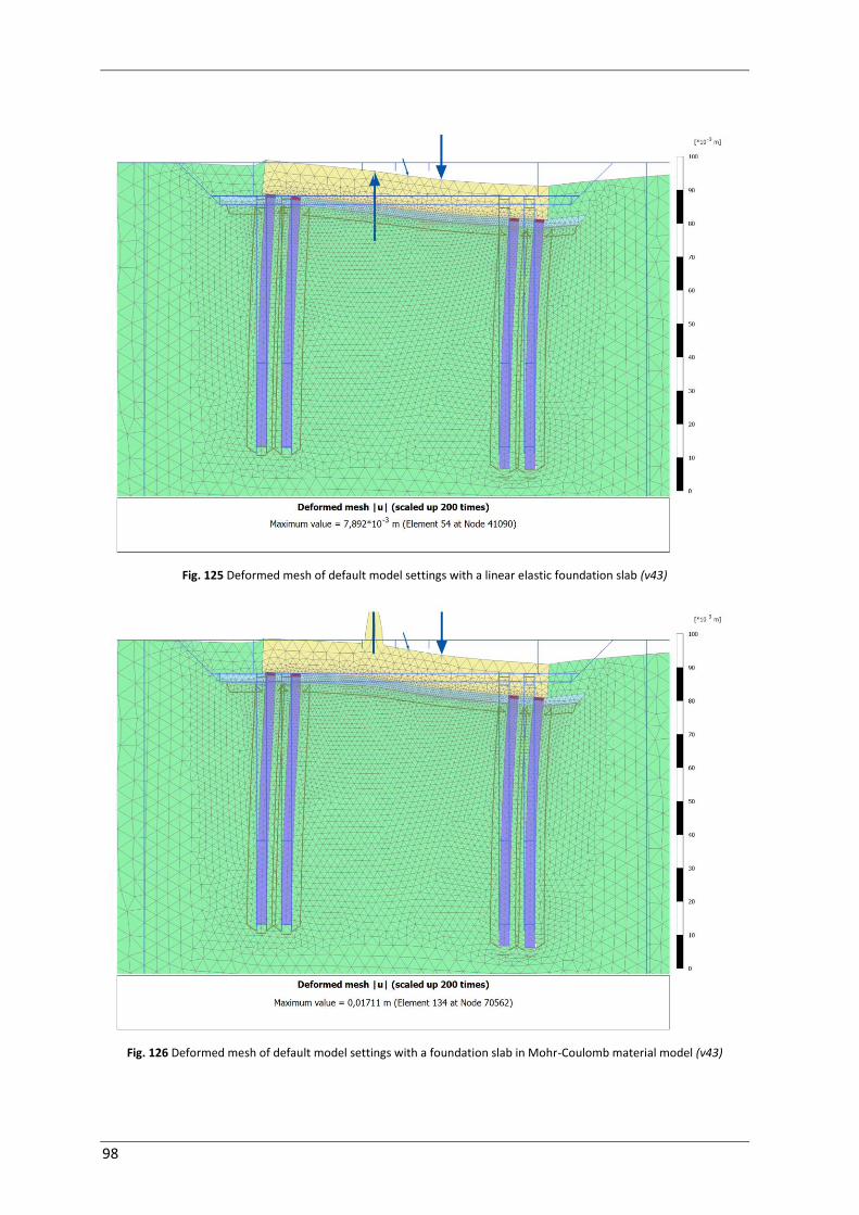
98

Fig. 125 Deformed mesh of default model settings with a linear elastic foundation slab (v43)

Fig. 126 Deformed mesh of default model settings with a foundation slab in Mohr-Coulomb material model (v43)

99

Fig. 127 Deformed mesh of default model settings with a foundation slab in Mohr-Coulomb material model with plates

for load application (v43)

100

Column 1.2

Column 1.2

Column 6.2

Column 6.2

Fig. 128 Utilisation in compression and tension of column 1.2 (left) and column 6.2 (right) with loading 3

(v01.42)

NUMERICAL ANALYSIS OF A FOUNDATION OF A WIND POWER …

Documents