This Working Paper is part of a research initiative on ‘Financial Inclusion’ carried out jointly by NSE and the Institute for Financial Management and Research (IFMR), Chennai. The views expressed in this Working Paper are those of the author(s) and do not necessarily represent those of NSE or IFMR. NSE-IFMR ‘Financial Inclusion’ Research Initiative 2014–2015 NSE Working Paper Series No. WP-2014-2 How Much Can Asset Portfolios of Rural Households Benefit from Formal Financial Services? Vishnu Prasad, Anand Sahasranaman, Santadarshan Sadhu, Rachit Khaitan

Welcome message from author
This document is posted to help you gain knowledge. Please leave a comment to let me know what you think about it! Share it to your friends and learn new things together.
Transcript

This Working Paper is part of a research initiative on ‘Financial Inclusion’ carried out jointly by NSE and the
Institute for Financial Management and Research (IFMR), Chennai. The views expressed in this Working Paper
are those of the author(s) and do not necessarily represent those of NSE or IFMR.
NSE-IFMR
‘Financial Inclusion’
Research Initiative
2014–2015
NSE Working Paper Series No. WP-2014-2
How Much Can Asset Portfolios of Rural
Households Benefit from Formal Financial Services?
Vishnu Prasad, Anand Sahasranaman, Santadarshan Sadhu, Rachit Khaitan

1
How Much Can Asset Portfolios of Rural
Households Benefit from Formal Financial Services?
Prepared by: Vishnu Prasad, Anand Sahasranaman, Santadarshan Sadhu, Rachit Khaitan
*
Abstract
Despite a demonstrated demand for various financial services, this paper finds that the asset portfolio
of the average rural household in India is composed almost entirely of two physical assets—housing
and jewellery. A comparison with a hypothetical portfolio of financial assets reveals that rural
households could earn significantly higher levels of real returns—an increase of 2.02% to 4.97%—at
the extant levels of risk. Our results point to the urgent policy imperative to provide rural households
with access to financial instruments that would allow them to construct a more diversified, tradable,
and liquid portfolio offering higher yields and shelter from local market fluctuations.
* The authors work at the IFMR Finance Foundation. The authors would like to thank Nachiket Mor, Bindu
Ananth, Kshama Fernandes, Bama Balakrishnan, Vaibhav Anand, Ravi Saraogi, Ratul Lahkar, and the
participants of the NSE-IFMR Conference 2014 for their valuable comments and guidance. The authors would
like to thank Nishanth K. for research assistance. Comments on the paper may be directed to

2
CONTENTS
Section 1 Introduction 4
Section 2 Literature Review 5
Section 3 Data and Methodology 7
Section 4 Data Summary: Asset Portfolios of Rural Households 10
4.1 Agricultural & Allied-Only 14
4.2 Labour-Only 14
4.3 Salaried and Agriculture & Allied 14
4.4 Business and Agriculture & Allied 14
4.5 Labour and Agriculture & Allied 15
Section 5 Assessment of Current Asset Portfolios 15
5.1 Land 15
5.2 Livestock 17
5.3 Gold 18
Section 6 Portfolio Risk-Return on Current Assets 19
Section 7 Assessment of Hypothetical Portfolios with Financial Assets 19
7.1 Insurance 19
7.2 Hypothetical portfolio of financial assets 21
Section 8 Policy Implications 27
8.1 Mutual funds 27
8.2 National Pension Scheme-Swavalamban 28
8.3 Distribution channel 30
Section 9 Conclusions 31
Appendices 34
Bibliography 37
List of Tables
Table 1: Brief Description of RFI Data 8
Table 2: Mean Household-Level Annual Income by Income Quintiles (in INR) 9
Table 3: Stylised Asset Portfolio of a Household 11
Table 4: Stylised Asset Portfolios 13
Table 5: Annual Returns and Standard Deviation on Assets 19
Table 6: Annual Returns and Standard Deviation of Stylised Portfolios 19
Table 7: Annual Returns and Standard Deviation on Assets (with Insurance) 20
Table 8: Annual Returns and Standard Deviation on Stylised Portfolios (with Insurance) 20
Table 9: Annual Returns and Standard Deviation on Financial Assets 22

3
Table 10: Comparison of Returns on Portfolio of Physical and Financial Assets 23
Table 11: Comparison of Returns on Portfolio of Physical and Financial Assets
including NPS 25
Table 12: Comparison of Sharpe Ratio of Asset Portfolios of Physical and Financial
Assets 26
List of Figures
Figure 1a: Classification of Households by Primary Occupational Categories 12
Figure 1b: Classification of Households by Secondary Occupational Categories 12
Figure 2: Efficiency Frontier with and without Insurance 21
Figure 3: Efficiency Frontiers of Physical Assets and Financial Assets 24
Figure 4: Efficiency Frontier with NPS 26

4
How Much Can Asset Portfolios of Rural Households
Benefit from Formal Financial Services?
1. Introduction
Despite a demonstrated demand for financial services (ranging from emergency loans for
consumption smoothing to a recurring deposit account), the penetration of formal financial
products in the asset portfolio of rural households in India remains extremely low. An
estimate suggests that only 32% of rural residents in India have a bank account (RBI, 2014b).
Anecdotal evidence suggests that the asset portfolio of rural households is dominated by
highly illiquid, non-tradable, and localised assets (such as land and housing) and varying
degrees of ownership of gold. For instance, the financial savings of households as a
percentage of the Gross Domestic Product (GDP) fell from approximately 12.5% in 2005–
2006 to 7% in 2012–2013, while the investment in physical savings and valuables (including
gold) increased from 12.5% to 14% and from 7.5% to 16%, respectively, over the same time
period (RBI, 2014a).
Capital markets offer various instruments that can effectively serve as diversification tools
against local market fluctuations; they also increase the choice set for rural investors.
Therefore, it is important to understand whether and how rural households can gain from
increased penetration of formal financial products in their asset portfolios. However, there is
a lack of clear understanding of the various components that constitute the portfolio of an
average rural household. In this context, this paper explores the composition of the asset
portfolios of rural households in India and assesses the extent to which rural households can
benefit from the introduction of financial market instruments into their asset portfolios.
Using customer data from a financial services institution that operates in five remote rural
districts (Arilayur, Pudukkottai, and Thanjavur in Tamil Nadu; Ganjam in Odisha; and Tehri
Garhwal in Uttarakhand) of India, we construct stylised typologies of household asset
portfolios based on primary and secondary sources of income. We then compare the
performance of these stylised portfolios over time with the performance of a hypothetical
portfolio that introduces financial instruments such as equity, insurance, index funds,
government securities, and the National Pension Scheme (NPS), which offer households
access to a more diversified and liquid asset portfolio. We compare these portfolios to assess

5
the change in the financial outcome of the households as a result of the introduction of
financial assets.
The remainder of this paper is organised as follows. Section 2 presents a brief review of the
relevant literature. Section 3 describes in detail the data and the methodology that the paper
employs. Section 4 examines the current composition of the asset portfolios of rural
households. Sections 5 and 6 provide an assessment of the portfolio of physical assets and
replacement financial assets, respectively. Section 7 discusses the policy implications of our
findings, and Section 8 concludes the paper.
2. Literature Review
As Campbell (2006) noted, households typically face long but finite planning horizons; a
large portion of the household asset portfolio is composed of non-tradable and illiquid assets
in the form of human capital and housing, respectively, and households often face significant
constraints on borrowing. A review of the literature on the portfolio allocation of household
assets reveals the following.
i. Households actively manage their asset portfolios, even in the absence of access to
formal financial markets
The evidence from literature suggests that households actively manage their asset portfolios
and employ a variety of risk diversification strategies. For example, Aryeetey (2004) found
that farm households in Ghana diversify their source of employment as a risk mitigation
strategy. Ghanaian farm households draw almost half of their total income from non-farm
self-employment and wage labour. Farm households are also known to diversify crops as a
risk mitigation strategy (Townsend, 1993). Rosenzweig and Wolpin (1993) found that
agricultural investment decisions by rural households are motivated by the need to smooth
consumption in the face of uncertain income streams. They found that households use certain
productive farm assets (such as bullocks) in their asset portfolio as a hedge against rainfall
risk. Fafchamps and Pender (1997) found that rural farm households in India treat irreversible
and reversible investments differently. Households refrain from investing in irreversible
investments—investments that cannot be readily reversed into liquidities—such as a well
because it restricts their ability to self-insure against external shocks. Households also
actively utilise informal financial mechanisms to manage their asset portfolios. Collins et al.
(2009) tracked the “financial diaries” of 250 households over a year and found that low-

6
income households use a wide range of financial instruments. The average number of unique
instruments used by households in India was eight. Households in the sample relied heavily
on informal savings and loan clubs—such as Rotating Savings and Credit Associations
(ROSCAs)—to tide over the “triple whammy” of low incomes, irregular cash flows, and
absence of suitable financial tools. Moreover, households frequently entered into reciprocal,
contractual relationships with one another as a method of risk pooling. For instance,
households in South Africa invest in a type of “funeral insurance,” in which premiums are
paid into informally created, group-run neighbourhood societies.
ii. Household asset portfolios are diverse, simple, and predominantly invested in low-
risk assets
McCarthy (2004) reported three key observations from a review of the empirical studies on
household portfolios. First, different households hold diverse asset portfolios. The asset
portfolios of households vary based on a number of variables including the country of
residence and wealth, as well as variables such as age, education, and the birth years of the
members. For example, across countries, richer households are more likely to hold risky
assets such as stocks, shares, property that is rented out, and family business. Second, with
the exception of housing, the average household asset portfolio is predominantly invested in
low-risk assets including savings and checking accounts, time deposits, and life insurance.
Third, the majority of the households hold portfolios that consist of fewer than five asset
types. The modal number of assets in the portfolios of households in the US was five.
iii. Investment in housing crowds out investments in other financial assets
Housing forms an important component of asset portfolios of households across countries.
Evidence from literature suggests that investments in housing could crowd out investments in
other financial assets. Cocco (2000) found that investment in housing is a significant driver of
the asset portfolio choice of households, especially for younger investors and households
with lower net worth. For these households, investment in housing keeps the overall liquidity
low, and thus, crowds out investment in stockholding. Flavin and Yamashita (2002) found
that the ratio of housing to net worth of the household declines over the life cycle of the
household. Younger households have a relatively large portion of their entire portfolio
invested in housing and are highly leveraged. This leads them to invest in less risky
investments such as bonds and to use their net worth to pay for their mortgage. As
households age, they accumulate wealth, thereby reducing the ratio of housing to net worth of

7
their portfolio. Similarly, Curcuru et al. (2004) found that the probability of stock ownership
decreases with an increase in the ratio of home equity to net worth. They argued that the
negative relation between stock holdings and real estate is consistent with a substitution
effect—for a given level of wealth, households that choose to spend more on housing have
less to invest in other assets. Chetty and Szeidl (2004) found that a USD 1 increase in
mortgage size leads to a 50–70% shift in portfolio allocation from stocks to bonds. However,
unlike other studies that suggested that this shift to safer assets is due to the increased
exposure to housing risk, they proposed that this shift occurs because housing is inherently a
“commitments” good—a good on which a transaction cost must be paid to shift consumption.
iv. There are discrepancies between ideal and observed financial behaviour of
households
Campbell (2006) suggested that there are discrepancies between the findings of positive
household finance (what households actually do) and normative household finance (what
households ought to do). For instance, household portfolios are typically analysed within the
framework of lifecycle models, which postulate that households follow a “hump-shaped”
asset accumulation pattern. The hump-shaped pattern suggests that households build up their
asset portfolios over their working years and draw upon them after retirement. Poterba and
Samwick (2001) challenged the central assumption of lifecycle models and found that all
assets within the asset portfolio need not follow the hump-shaped pattern. For instance, the
ratio of financial assets to total assets declines as the household ages and subsequently
increases at later ages. Further, the study found significant “cohort effects” that determine
asset portfolio choice. For instance, in the US, while baby boomers demonstrate average
propensity to hold taxable equity and hold an average share of taxable equity in their
portfolio, younger cohorts have larger investment in bonds and tax-deferred accounts.
Additionally, younger cohorts leverage their assets to a larger extent than older cohorts do.
3. Data and Methodology
This paper analyses the asset portfolios of the customers of a Rural Financial Institution
(RFI)1 that provides financial products and services to remote rural households in India and
functions in areas where other formal financial institutions do not operate. As of September
2013, the RFI services approximately 2,25,000 households across five districts in three
1 The name of the institution has been withheld in order to ensure confidentiality.

8
different states, Tamil Nadu, Uttarakhand, and Odisha, and has a network of 201 branches.
The RFI aims to provide a complete suite of financial services to all individuals and
households in its service area. In doing so, it is guided by a wealth management approach that
ensures that products and services are recommended for a household based on an
understanding of its financial situation, asset allocation, risk tolerance, needs, and goals.
The RFI captures extensive details of the households that it enrols. On average, across all its
service areas, a branch enrols 56% of the households in its service area, thereby collecting
data on a representative cross-section of rural households. A brief description of the data
collected by the RFI is provided in Table 1.
Table 1: Brief Description of RFI Data
Household Details For each family member (including enrolee):
- Name, relationship to enrolled member, age, education
Family Income Income details for each family member, with provision for incomes to be
recorded from multiple sources per member:
- Income-generating activities the member is involved in, net income from
the activity, frequency of income, duration of income
Family Expenditure Expenditure amounts and frequency for:
- Clothing, education, fees, electricity, festival, food, health, house rent,
insurance, shop rent
Assets - House: number of houses, build type, roof type
- Shop: number of shops, build type, roof type
- Land ownership and usage: area under cultivation for different crops;
non-irrigated land, irrigated land
- Number and type of agriculture equipment
- Livestock
- Electronic goods
- Vehicle(s)
- Jewellery (quantity)
Liabilities For existing loans:
- Source, amount, frequency, instalment amount, tenure
Household Goals For the household’s goals related to marriage, education, loan repayment,
house, land, gold, business, other assets, other expenses:
- Family member to whom the goal is to be mapped
- Number of years in which to achieve the goal
- Amount of money stipulated for the goal
- Change in surplus as a result of the goal being added to the household’s
finances
The mean household-level annual income of the RFI’s customers classified by income
quintiles is provided in Table 2. A household in the first income quintile has a self-reported
annual income of INR 41,452, while a household in the fifth income quintile earns INR
3,56,277.

9
Table 2: Mean Household-Level Annual Income by Income Quintiles (in INR)
For the purpose of this paper, we analyse the asset portfolios of a set of 1,43,632 households.2
Segregated by region, 69% of the sample households reside in Tamil Nadu, while Odisha and
Uttarakhand account for 19% and 12% of the households, respectively. As explained in Table
1, the RFI collects data pertaining to household investments in nine asset categories—
agricultural equipment, electronic goods, housing, investment (in the NPS and Money Market
Mutual Funds), jewellery, land, livestock, shop (or business), and vehicles. We further
categorise these assets into two groups—consumption assets and investment assets.
Consumption assets are defined as those assets whose value is consumed or drawn down over
the lifecycle of the asset. This category comprises electronic goods, housing, and vehicles.
While housing is traditionally viewed as an investment, we classify it as a consumption asset
on the premise that its intrinsic value is distinct from that of the land on which it is situated.
This is substantiated by its illiquid character owing to the lack of well-functioning housing or
rental markets in the regions in which the RFI operates. Thus, we assume that the value of
housing also comes down over time. Investment assets, on the other hand, are defined as
productive assets and/or assets that are actively managed in household portfolios. Appendix 1
provides a detailed description of the data collected under each asset category and the per unit
value assigned to them. The unit value of an asset is based on self-reported information.
Currently, the data does not take into account regional variation in the price of assets such as
land, housing, and shops/commercial establishments. Further, per unit values of housing and
shop(s) are based on their build and roof types only.
We use this data to construct stylised household asset portfolios that are stratified based on
source of income (primary and secondary). Using the tools of Modern Portfolio Theory
(MPT), we then compare the performance of the stylised portfolios over time with the
performance of a hypothetical portfolio that offers these households access to a suite of
financial instruments such as Exchange Traded Funds (ETFs), savings bank accounts,
insurance, government securities, index funds, and the NPS, which provides households a
2 The number of households in our sample is smaller than the universal set of 2,25,000 households, as
households with asset values in the top 5 percentile of each asset category were considered outliers and
removed.
Income
Quintile
1
Income
Quintile 2
Income
Quintile 3
Income
Quintile 4
Income
Quintile 5
Annual Household Income 41,452 80,788 118,162 169,840 356,277

10
more diversified and liquid asset portfolio. For the purpose of this paper, we quantify the
financial gain to five stylised occupational categories from a limited suite of seven financial
assets.
The foundations of the MPT were laid by Markowitz (1952) when he modelled the behaviour
of a rational investor under uncertainty. The MPT laid the platform for various developments
in modern finance including the Capital Asset Pricing Model (CAPM), which was developed
by Sharpe (1964) and Lintner (1965). The MPT, for the first time, mathematically articulated
the idea of portfolio diversification that allowed investors to select a portfolio of assets that in
combination has a level of risk lower than that of the individual assets contained in the
portfolio.
Despite the various criticisms of the MPT,3 the fundamental principle behind Markowitz’s
seminal paper rings true even today:
Not only does the E-V [expected returns-variance of returns] hypothesis imply
diversification, it implies the “right kind” of diversification for the “right
reason.”' The adequacy of diversification is not thought by investors to depend
solely on the number of different securities held. A portfolio with sixty
different railway securities, for example, would not be as well diversified as
the same size portfolio with some railroad, some public utility, mining,
various sorts of manufacturing, etc. The reason is that it is generally more
likely for firms within the same industry to do poorly at the same time than for
firms in dissimilar industries.
Similarly in trying to make variance small, it is not enough to invest in many
securities. It is necessary to avoid investing in securities with high covariances
among themselves. We should diversify across industries because firms in
different industries, especially industries with different economic
characteristics, have lower covariances than firms within an industry.
(Markowitz, 1952: 89)
4. Data Summary: Asset Portfolios of Rural Households
In this section, we provide an in-depth examination of the current asset portfolios of rural
households based on the RFI’s data. Table 3 presents the case of a household whose stylised
asset portfolio is composed of median holdings of each asset category. The total net worth of
this household is INR 2 lakh. Consumption assets form 54% of the entire asset portfolio of
3 For an excellent review of the history of the MPT, see Elton and Gruber (1997). For a more systematic critique
and introduction to competing theories, see Sortino and Satchell (2001).

11
the stylised household, and jewellery4 (44%) is the predominant investment asset. As
suggested by our review of extant literature and anecdotal evidence presented earlier, two
assets—jewellery and housing—form 93% of the total net worth of the average rural
household.
Table 3: Stylised Asset Portfolio of a Household
Asset Category Median Value (in
INR)
Percentage
of Total
Assets
Electronics 7,000 3.49%
House 99,000 49.36%
Vehicle 1,250 0.62%
Consumption assets (total) 107,250 53.47%
Agricultural equipment 500 0.25%
Investment - 0.00%
Jewellery 88,320 44.03%
Land - 0.00%
Livestock 4,500 2.24%
Shop - 0.00%
Investment assets (total) 93,320 46.53%
All assets (total) 200,570 100.00%
We examined the various stylised households stratified based on source of income. Figures
1a and 1b show the frequency distribution of the entire sample (1,43,632 households) based
on:
i. The household’s primary source of income, i.e., the source that is the highest
contributor to total household income.
ii. The secondary source of income, i.e., the source that is the second-highest
contributor to total household income.
Based on reported source of income, we classified households into nine occupational
categories, viz. Agriculture & Allied; Business; Salaried; Labour; Professional; Migrant;
Working Abroad; Non-earned; and Unpaid/unemployed. Appendix 2 presents the specific
occupations that comprise each occupational category. For example, “non-earned” consists of
those households that earn their primary source of income without the direct use of their
human capital, i.e., from rental housing or from retirement assets. “Unpaid/unemployed”
comprise households whose primary breadwinners are students, house-wives, or the
unemployed.
4 Jewellery in this context refers to gold jewellery only.

12
Figure 1a shows that just over half of the households (51%) in our entire sample rely on
labour as their primary source of income, while 15% rely on agriculture and allied activities,
13% on business, and 12% on salaried employment. Figure 1b shows that more than half
(56%) of all households in our sample do not have a secondary source of income. This
suggests that at a household level, their income streams are not very diversified, i.e., the
households have concentrated exposure to a particular occupation. Further, 19% of all the
households have agriculture and allied activities as a secondary source of income while 15%
have labour.
Figure 1a: Classification of Households by Primary Occupational Categories
Figure 1b: Classification of Households by Secondary Occupational Categories
50.65%
14.88%13.00% 11.67%
6.34%
1.58% 0.80% 0.77% 0.31%
56.10%
18.66%
14.72%
4.83%2.96%
0.81% 0.79% 0.71% 0.41%

13
We used the nine occupational categories described in Figures 1a and 1b to construct stylised
asset portfolios that are segregated by primary source of income. For the purpose of this
paper, we restricted our analysis to five stylised occupational typologies that are stratified
based on sources of primary and secondary income, which represent 63% of the households
in our sample:
i. Labour (primary) and no secondary occupation
ii. Agriculture & allied (primary) and no secondary occupation
iii. Salaried (primary) and agriculture & allied (secondary)
iv. Business (primary) and agriculture & allied (secondary)
v. Labour (primary) and agriculture & allied (secondary)
The asset portfolio of each occupational category is composed of the median holding of an
asset for that occupational category. For example, the stylised asset portfolio of a business
household is composed of median asset values of all business households.5 The five stylised
portfolios are presented in Table 4.6
Table 4: Stylised Asset Portfolios
Asset category
Agriculture-
Only
Labour-
Only
Salaried-
Agriculture
Business-
Agriculture
Labour-
Agriculture
Electronics 7,000 7,000 7,000 7,000 7,000
House 99,000 63,000 225,000 225,000 99,000
Vehicle 1,250 1,250 - - 1,250
Consumption assets (total) 107,250 71,250 232,000 232,000 107,250
Agricultural-equipment 2,500 - 5,500 5,500 2,000
Investment - - - - -
Jewellery 110,400 66,240 64,384 96,576 66,240
Land 200,000 - 130,000 140,000 120,000
Livestock 20,000 300 25,000 25,000 20,300
Shop - - - - -
Investment assets (total) 332,900 66,540 224,884 267,076 208,540
Investment assets (as % of all assets) 75.63% 48.29% 49.22% 53.51% 66.04%
All assets (Total) 440,150 137,790 456,884 499,076 315,790
We now examine the asset portfolio of the five stylised occupational typologies.
5 Appendix 3 summarises the stylised asset portfolios of all nine occupational categories and compares these
portfolios with the portfolio of the median stylised household presented in Table 3. 6 The value of land for the median household presented in Table 3 is zero since the median household is a
labour-only household. However, as shown in Table 4, other stylised households have a positive median value
for land.

14
4.1 Agricultural & Allied-Only
The agricultural and allied occupational category comprises 15% of the overall sample of
rural households and contains households whose primary source of income originates from
agriculture, agricultural trading, dairy, and fishing. Of these households, 60% are households
whose sole source of income is from agriculture and allied activities. This occupational
category is distinguished by the large proportion of investment assets in the total asset
portfolio. Compared to a sample average of 46%, this category holds 75% of the total
portfolio in the form of investment assets. This occupational category also has the largest
median holdings of jewellery and land in the sample.
4.2 Labour-Only
Labour households—defined as those households that are engaged in wage labour or are
employed as drivers—form 51% of the entire sample of rural households. Among these
households that are engaged in labour as their primary source of income, the largest
proportion (76%) do not have another source of income. Labour-only households are the
poorest in terms of net worth in the entire sample of households. These households are
heavily invested in jewellery, but the value of their consumption assets exceeds that of their
investment assets.
4.3 Salaried and Agriculture & Allied
The salaried occupational category is composed of households whose primary source of
income is salaried employment. Most salaried households (76%) have a secondary source of
income, and a majority (39%) are engaged in agriculture and allied activities. The salaried-
agriculture occupational category has median holdings of livestock and agricultural
equipment that exceed the holdings of agriculture-only households. These households are
also heavily invested in housing assets. The fact that a large majority of salaried households
have a secondary occupation could be explained as a risk mitigation measure in the absence
of financial tools to do the same.
4.4 Business and Agriculture & Allied
The business occupational category accounts for 13% of the overall sample and is composed
of households whose primary breadwinner is a shop owner, or the owner of a small industry,

15
or is engaged in other businesses. Surprisingly, therefore, the median holding of shop or
family-owned business for this asset category is zero. The higher-than-median holdings of
agricultural equipment, livestock, and land suggest that this category derives a significant
portion of their income from agriculture and allied activities; 35% of all business households
are engaged in agriculture and allied activities for their secondary source of income. This
category is also the richest in the sample in terms of net worth.
4.5 Labour and Agriculture & Allied
The labour-agriculture combined occupational category constitutes 14% of all labour
households. Labour-agriculture households have a significantly higher net worth compared to
other labour households. This is driven most significantly by their investment in land and
livestock. Their holding of housing assets is also the highest within the labour category.
5. Assessment of Current Asset Portfolios
We assess the performance of the five selected asset portfolios presented in Table 4 over
time. As seen earlier, three assets—land, jewellery (gold), and livestock—constitute the
entirety of investment assets for most households. In order to assess the performance of these
assets over time, we use historical gold price data and construct cash-flow models for land
and livestock. Both models are discussed in detail below.
5.1 Land
Price data on land transactions in India is difficult to obtain due to three primary reasons.
First, the absence of unified state-level land registries makes transaction data on land
extremely difficult to obtain. The most comprehensive study on Indian land markets that we
could find was GIZ (2014), which collected data on land transactions for a period of thirty
years in four districts of Haryana and Madhya Pradesh. By the study’s own admission,
“merging the data collected from the four districts for a period of 30 years yielded close to
6,80,000 lines of entry” (GIZ, 2014: 13). Such an exercise for the districts in our sample was
beyond the scope of this study. Second, as Chakravorthy (2013: 169) observed, “official
records often understate the actual prices, primarily to underpay stamp duties. Many states
have pre-emptively set stamp duty rates (by zones, grades etc.) to get around this problem,
but all that means is buyers and sellers know what official price to declare, which is not
necessarily the true transaction price.” Third, even if true transaction prices could be

16
obtained, the reservation price of land would remain unknown. As several studies have found,
many instances of land sales are instances of distress sales. For example, Patil and Marothia
(2009) observed that in the state of Chhattisgarh, marginal landowners obtain only a third of
the price for their land when compared to larger landowners. Many households sell land as a
measure of last resort, especially in the absence of sufficient access to credit.
On account of these difficulties, we resorted to a theoretical estimation of the price of land.
The underlying assumption of our model, based on Chakravorthy (2013), is that “land is like
all other income-producing assets—its value is determined solely by the income it can
produce—and a sale is possible only if a buyer’s valuation of the discounted future income
stream is more than the seller’s valuation of the same.” In order to estimate the cash flows
from holding land as an asset, we made the following assumptions:
1. The sole use of land is agricultural.
2. The lifetime of land as an asset is 50 years.
3. Capital gain from the sale of land at the end of its lifetime is zero.
4. The model does not take into account regional variations in agricultural productivity.
The internal rate of return (IRR) is projected based on mean all-India values.
5. The present value of an acre of land is INR 2 lakh.
Chakravorthy (2013) estimated the price of land based on output per acre (2003–2006) of a
basket of 44 crops for 17 states in India. The average value of output per acre for India is
estimated to be INR 14,543 (2012–2013 prices). Based on Foster and Rosenzweig (2011), we
assumed that profit or income per acre of land is 35% of the value of the output. Further, we
assumed that agricultural productivity increases at a CAGR of 2.35%, based on Bhalla and
Singh (2010). In our model, output per acre is dependent only on the average rainfall received
during the year; based on Blignaut et al. (2009), we assumed that a 1% deviation from mean
historical rainfall would lead to a 1% decline in the value of output per acre. If the rainfall in
any year varied in excess of one standard deviation above or below the mean historical
rainfall, we assumed that the farmer lost the entire value of his/her crop.7 Based on data
available from the Indian Institute of Tropical Meteorology, mean all-India annual rainfall
between 1813 and 2006 was 1150.49 mm, with a standard deviation of 110.59 mm.8 Finally,
7 The Indian Institute of Tropical Meteorology classifies years of flood and drought using this methodology.
Available at: http://www.tropmet.res.in/~kolli/MOL/Monsoon/Historical/air.html. 8 Available at http://www.tropmet.res.in/Data%20Archival-51-Page

17
we simulated the IRR and standard deviation on holding land as an asset based on 10,000
Monte Carlo trials.
5.2 Livestock
The cash flows from holding livestock were projected for a stylised median household to
estimate the returns and risk on such an investment. This was based on primary information
collected from a para-veterinarian for a large insurance company. The median household
owns INR 20,000 worth of livestock, the value of which corresponds to that of an Ongole
breed cow.9 The cash flows were projected for a 10-year time frame, based on the estimated
life expectancy of this breed of cow. Further, we assumed that the household makes this
investment at the beginning of the cow’s lifetime.
In terms of revenue streams, the following were taken into account:
1. Milk: The revenue from milk was estimated based on primary information collected
about the daily peak yield of milk and yearly peak yield factors of an Ongole breed
cow, as well as the price of milk.
2. Manure: Revenue from manure was estimated based on primary information
collected about the value of manure generated per week.
3. Calf: Our model assumed that there is a 50% probability of a maximum of one calf
being born to a cow each year between the third and eighth years of its lifetime, with a
maximum of six calves during its lifetime. Further, we assumed that the calf is sold as
soon as it is born for the value at which the cow was purchased, i.e., INR 20,000.
4. Terminal value: Our model assumed that there is no value for the cow’s meat,
carcass, or any other part at the end of its lifespan.
In terms of costs, the following were taken into account:
1. Purchase price of asset: This represents the initial one-time cash outflow, which in
our model was taken to be INR 20,000 (which corresponds to the market price of an
Ongole cow).
2. Fodder costs: The cost of fodder was estimated based on primary information
collected about the daily consumption, the cost per kilogram, and the proportions of
dry fodder, green fodder, and concentrated feed.
9 Description of Ongole breed cow: http://www.ansi.okstate.edu/breeds/breeds/cattle/ongole/index.htm.

18
3. Medical costs: Medical expenses included the annual costs of periodic deworming
and vaccination.
4. Insemination costs: Based on the probability of the birth of a calf, our model
assumed the cost for insemination in the year before a calf is born.
5. Treatment expenses: This was based on the estimated cost of treating an incidence
of foot and mouth disease.
6. Labour costs: Our model did not take into account the cost of labour required for the
upkeep of the cow.
The model assumed that the only sources of risk were those associated with the morbidity
(incidence of foot and mouth disease) and/or death of the animal during its 10-year lifetime.
These were taken into account by simulating the state of the cow (alive or dead; if alive:
healthy or unhealthy) from a binomial distribution, based on the mortality and morbidity rates
estimated through primary research conducted by Bangar et al. (2013) in Maharashtra.
Finally, the internal rate of return (IRR) was computed for 10,000 trials of the ensuing
simulated cash flows.
While other studies such as Anagol et al. (2013) found low to negative returns and Attanasio
& Augsburg (2014) found high returns on the ownership of a cow in India, the model in this
paper differs in its calculation of returns over the entire lifetime of a cow, even without taking
into account labour costs. Additionally, our model accounts for the risk associated with the
mortality and morbidity of a cow, although not in the case of drought (or deviation from
mean rainfall).
5.3 Gold
Returns on gold (jewellery) were estimated based on actual gold price time series data from
MCX for the period 2003–2014.10
Table 5 presents the mean projected return and standard
deviation on land, jewellery (gold), and livestock.
10
Available at http://www.mcxindia.com/sitepages/HistoricalDataForVolume.aspx.

19
Table 5: Annual Returns and Standard Deviation on Assets
Jewellery
(Gold) Land Livestock
Annual Returns 14.64% 2.35% 10.26%
Standard
Deviation 18.70% 0.21% 17.86%
6. Portfolio Risk-Return on Current Assets
Based on the estimated mean annual returns and risk (standard deviation) on assets, we
estimated the weighted return and risk of five stylised household asset portfolios.11
This is
presented in Table 6.
Table 6: Annual Returns and Standard Deviation of Stylised Portfolios
Agriculture-
Only
Labour-
Only
Salaried-
Agriculture
Business-
Agriculture
Labour-
Agriculture
Annual Returns 6.93% 14.62% 6.86% 7.64% 7.07%
Standard Deviation 6.13% 18.60% 5.48% 6.79% 5.92%
Based on our projections, the stylised asset portfolio of labour-only households—composed
almost entirely of jewellery—realised the best returns over time: 14.63%, with a
corresponding portfolio risk (standard deviation) of 18.60%. The portfolio of business-
agriculture households realised annualised returns of 7.64% with a standard deviation of
6.79%. The asset portfolios of salaried-agriculture as well as labour-agriculture households
realised annual returns of 6.86% and 7.07%, respectively. Although providing comparable
returns (6.93%), the portfolio risk of agriculture-only households remained marginally higher
at 6.13% compared to that of salaried-agriculture (5.48%) and labour-agriculture households
(5.92%).
7. Assessment of Hypothetical Portfolios with Financial Assets
7.1 Insurance
We now compare the projected performance of these asset portfolios with a set of
hypothetical portfolios that introduces financial instruments that offer risk mitigation. Table 7
shows the modified annual returns and risk of holding land and livestock with two additional
11
As explained in Section 5, the returns and standard deviation on land and livestock were simulated
individually, without taking their correlation with other local assets into consideration. As a result, the returns
and standard deviation on physical assets did not take the effect of local, systematic risks into account and
could, therefore, be over-estimated in our analysis.

20
products—rainfall and livestock insurance. Table 8 compares the extant asset portfolio of
households with a hypothetical portfolio in which households have these two additional
products.
Livestock insurance involved the following factors:
a. An annual premium payment of 5% of the initial value of the cow.12
b. A pay-out of 100% of the initial value of the cow in the event of its death, as
described in the risk consideration above.
Rainfall insurance took into account the following factors:
a. An annual premium payment equivalent to 10% of the sum assured.13
The sum
assured is assumed to be the expected output per acre.
b. The pay-out from insurance is equivalent to the shortfall from expected output per
acre caused due to deviations from mean rainfall.
Table 7: Annual Returns and Standard Deviation on Assets (with Insurance)
Land Livestock
Annual Returns 2.52% 12.06%
Change in Returns 0.17% 1.80%
Standard
Deviation 0.00% 9.12%
Change in Risk -0.21% -8.74%
Table 7 shows that the introduction of rainfall insurance improves the returns on land
marginally by 0.17% and reduces standard deviation to zero. Livestock insurance improves
the returns on livestock by 1.80% and substantially reduces the risk due to the death of the
livestock by 8.74%.
Table 8: Annual Returns and Standard Deviation on Stylised Portfolios (with Insurance)
Agriculture-
Only
Labour-
Only
Salaried-
Agriculture
Business-
Agriculture
Labour-
Agriculture
Annual Returns 7.15% 14.63% 7.16% 7.91% 7.35%
Change in Returns 0.22% 0.01% 0.30% 0.27% 0.28%
Standard Deviation 6.21% 18.61% 5.47% 6.86% 5.96%
Change in Risk 0.08% 0.01% -0.01% 0.07% 0.04%
Table 8 demonstrates that with the introduction of two additional products—rainfall and
livestock insurance—all the stylised households (except labour-only households) realise
12
The annual premium rate was based on observed market rates. 13
The annual premium rate was based on observed market rates.
21
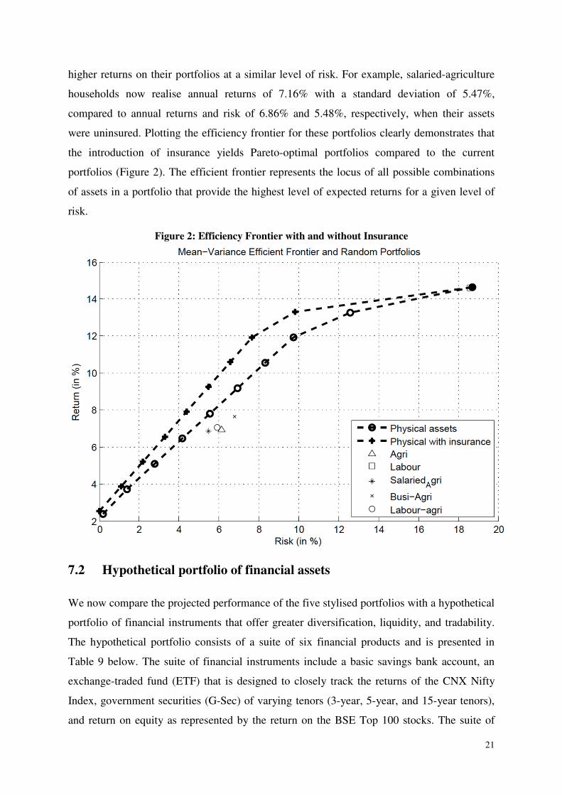
higher returns on their portfolios at a similar level of risk. For example, salaried-agriculture
households now realise annual returns of 7.16% with a standard deviation of 5.47%,
compared to annual returns and risk of 6.86% and 5.48%, respectively, when their assets
were uninsured. Plotting the efficiency frontier for these portfolios clearly demonstrates that
the introduction of insurance yields Pareto-optimal portfolios compared to the current
portfolios (Figure 2). The efficient frontier represents the locus of all possible combinations
of assets in a portfolio that provide the highest level of expected returns for a given level of
risk.
Figure 2: Efficiency Frontier with and without Insurance
7.2 Hypothetical portfolio of financial assets
We now compare the projected performance of the five stylised portfolios with a hypothetical
portfolio of financial instruments that offer greater diversification, liquidity, and tradability.
The hypothetical portfolio consists of a suite of six financial products and is presented in
Table 9 below. The suite of financial instruments include a basic savings bank account, an
exchange-traded fund (ETF) that is designed to closely track the returns of the CNX Nifty
Index, government securities (G-Sec) of varying tenors (3-year, 5-year, and 15-year tenors),
and return on equity as represented by the return on the BSE Top 100 stocks. The suite of
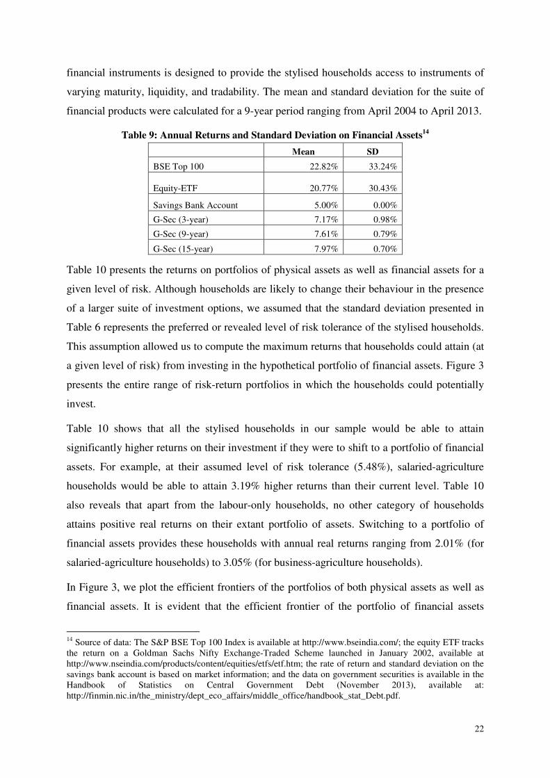
22
financial instruments is designed to provide the stylised households access to instruments of
varying maturity, liquidity, and tradability. The mean and standard deviation for the suite of
financial products were calculated for a 9-year period ranging from April 2004 to April 2013.
Table 9: Annual Returns and Standard Deviation on Financial Assets14
Table 10 presents the returns on portfolios of physical assets as well as financial assets for a
given level of risk. Although households are likely to change their behaviour in the presence
of a larger suite of investment options, we assumed that the standard deviation presented in
Table 6 represents the preferred or revealed level of risk tolerance of the stylised households.
This assumption allowed us to compute the maximum returns that households could attain (at
a given level of risk) from investing in the hypothetical portfolio of financial assets. Figure 3
presents the entire range of risk-return portfolios in which the households could potentially
invest.
Table 10 shows that all the stylised households in our sample would be able to attain
significantly higher returns on their investment if they were to shift to a portfolio of financial
assets. For example, at their assumed level of risk tolerance (5.48%), salaried-agriculture
households would be able to attain 3.19% higher returns than their current level. Table 10
also reveals that apart from the labour-only households, no other category of households
attains positive real returns on their extant portfolio of assets. Switching to a portfolio of
financial assets provides these households with annual real returns ranging from 2.01% (for
salaried-agriculture households) to 3.05% (for business-agriculture households).
In Figure 3, we plot the efficient frontiers of the portfolios of both physical assets as well as
financial assets. It is evident that the efficient frontier of the portfolio of financial assets
14
Source of data: The S&P BSE Top 100 Index is available at http://www.bseindia.com/; the equity ETF tracks
the return on a Goldman Sachs Nifty Exchange-Traded Scheme launched in January 2002, available at
http://www.nseindia.com/products/content/equities/etfs/etf.htm; the rate of return and standard deviation on the
savings bank account is based on market information; and the data on government securities is available in the
Handbook of Statistics on Central Government Debt (November 2013), available at:
http://finmin.nic.in/the_ministry/dept_eco_affairs/middle_office/handbook_stat_Debt.pdf.
Mean SD
BSE Top 100 22.82% 33.24%
Equity-ETF 20.77% 30.43%
Savings Bank Account 5.00% 0.00%
G-Sec (3-year) 7.17% 0.98%
G-Sec (9-year) 7.61% 0.79%
G-Sec (15-year) 7.97% 0.70%

23
completely dominates the portfolio of physical assets currently held by the stylised
households in our sample. This means that at any given level of risk, investment in a portfolio
of financial assets would provide a higher level of returns than investment in physical assets
would. By investing in financial instruments, the stylised households in our sample could
attain their present level of returns at a substantially lower level of risk.
Table 10: Comparison of Returns on Portfolio of Physical and Financial Assets
Agriculture-
Only
Labour-
Only
Salaried-
Agriculture
Business-
Agriculture
Labour-
Agriculture
Nominal Returns on
Portfolio of Physical Assets 6.93% 14.62% 6.86% 7.64% 7.07%
Real Returns on Portfolio of
Physical Assets15
-1.11% 6.58% -1.18% -0.40% -0.97%
Nominal Returns on
Portfolio of Financial
Assets 10.54% 16.64% 10.05% 11.09% 10.38%
Real Returns on Portfolio of
Financial Assets 2.50% 8.60% 2.01% 3.05% 2.34%
Change in Returns 3.61% 2.02% 3.19% 3.45% 3.31%
Standard Deviation 6.13% 18.60% 5.48% 6.79% 5.92%
Figure 3 also plots the individual portfolios of the five stylised households. Except for the
labour-only households, all the other households hold portfolios that are inefficient, even with
respect to a suite of assets that are currently accessible to them. This could partially be
explained by the lumpy nature of investment in physical assets (it is not possible to own half
a cow). The only stylised household whose portfolio lies on the efficient frontier is the
labour-only household category. However, it should be noted that labour-only households
adopt a high risk-high return strategy due to their over-investment in one asset, viz. gold. We
assume that rural households are forced to adopt a high risk-high return strategy due to two
reasons. First, rural households have access to a limited set of assets that they can use to
diversify their portfolio. Diversification by investment in land—the asset that is missing from
the portfolio of labour-only households—is precluded by the very nature of land being a
lumpy investment and the absence of a tradable rural land market. Second, labour-only
households are the poorest (in terms of net worth) households in our sample. Diversification
into land requires a substantial amount of investment and is unsuited to the requirements of
these households that often save in small amounts. Due to these two factors, labour-only
15
Mean annual inflation for the period 1983–2012 was 8.04%.

24
households are over-invested in one asset, leaving them singularly vulnerable to the risk of
adverse price fluctuations on that asset.
Figure 3: Efficiency Frontiers of Physical Assets and Financial Assets
The efficiency frontiers presented in Figure 3 are the result of an unconstrained optimisation,
i.e., we did not pre-determine a minimum or maximum holding value for any asset in the
portfolio. In Table 11, we estimate the portfolio returns on financial assets after the addition
of a long-term pensions saving product, represented by the National Pension Scheme (NPS).
According to our estimates, the NPS offers returns of 10.97% at a risk level (standard
deviation) of 2.40% over a lifecycle of 40 years. The mean and standard deviation on the
NPS were calculated based on a model that estimates the annual returns from the scheme.
The model assumed that the contribution to NPS is invested in three classes of assets—
equity, corporate bonds, and government securities—based on an age-linked investment
process called the lifecycle mix. The lifecycle investment mix varies the proportion of
investment in the three classes of assets according to the age of the customer and shifts
investments from riskier assets (80% of the contribution is invested in equity and corporate
bonds for a 20-year old) to safer instruments (80% is invested in government securities for a

25
55-year old) as the customer ages. The mean and standard deviation were calculated based on
10,000 trials of a Monte Carlo simulation.
Unlike the other financial assets in the portfolio, the NPS is not a tradable asset, but is a
critical component of the household’s asset portfolio from a long-term perspective. To
capture the nature of this investment, we imposed a constraint that forces households to
invest 20% of their portfolio in NPS. We found that at their assumed level of risk preference,
all the stylised households could gain a rate of return that is higher than the returns obtained
on the initial suite of six financial assets. Compared to their current portfolio of physical
assets, households could gain an increase in returns, ranging from 2.47% for labour-
agriculture households to 4.94% for agriculture-only households. In real terms, the annual
returns on portfolio range from 2.70% for salaried-agriculture households to 3.83% for
agriculture-only households.
Table 11: Comparison of Returns on Portfolio of Physical and Financial Assets including NPS
Agriculture-
Only
Labour-
Only
Salaried-
Agriculture
Business-
Agriculture
Labour-
Agriculture
Nominal Returns on
Portfolio of Physical Assets 6.93% 14.62% 6.86% 7.64% 7.07%
Real Returns on Portfolio of
Physical Assets -1.11% 6.58% -1.18% -0.40% -0.97%
Nominal Returns on
Portfolio of Financial
Assets (including NPS) 11.87% 17.09% 10.74% 11.73% 11.27%
Real Returns on Portfolio of
Financial Assets (including
NPS) 3.83% 9.05% 2.70% 3.69% 3.23%
Change in Returns 4.94% 2.47% 3.88% 4.09% 4.20%
Standard Deviation 6.13% 18.60% 5.48% 6.79% 5.92%
Table 12 compares the Sharpe ratio of the asset portfolios of physical and financial assets.
The Sharpe ratio measures the excess returns per unit of additional deviation in a portfolio of
assets, i.e., a risk-adjusted indicator of the performance of a portfolio. Table 12 shows that the
Sharpe ratio for portfolios of physical assets is negative, except for labour-only and business
agricultural households. A negative Sharpe ratio indicates that compared to the current
portfolio, the household is better off investing entirely in risk-free assets. Table 12 also
reveals the poorer quality of asset choice by labour-only households. Although their extant
portfolios offer them a high rate of return, the risk premium (as measured by the Sharpe ratio)
they obtain for taking additional risk is low compared to that of both portfolios of financial
assets.

26
Figure 4 plots the efficiency frontier of the portfolio of financial assets including NPS. At any
point on this efficient frontier, 20% of the household’s investment is held in NPS. We found
that the portfolios of financial assets with NPS yield Pareto-optimal results compared to both
the portfolio of physical assets as well as the limited suite of financial assets (without NPS).
Table 12: Comparison of Sharpe Ratio of Asset Portfolios of Physical and Financial Assets
Sharpe Ratio Agriculture-
Only
Labour-
Only
Salaried-
Agriculture
Business-
Agriculture
Labour-
Agriculture
Portfolio of Physical
Assets -3.92 40.05 -5.66 6.92 -1.69
Portfolio of
Financial Assets 54.98 50.91 52.55 57.73 54.22
Portfolio of
Financial Assets
including NPS
76.67 53.33 65.15 67.16 69.26
Figure 4: Efficiency Frontier with NPS
The gap between the efficient frontiers of physical assets and financial assets (plotted in
Figures 2, 3, and 4) represents the efficiency loss to rural households due to their exclusion
from the ambit of the formal financial system. It is clear that this exclusion prevents them
from realising higher returns on their investments by forcing them to invest in a limited range
of lumpy, illiquid, and non-tradable physical assets. As the case of labour-only households

27
reveals, the lack of diversification tools also forces households to assume an adversely risky
position. Further, the portfolio of physical assets provides a narrow range of risk-return
positions that rural households can assume in the market. While a complete substitution of
physical assets for financial assets may not be possible or desirable, it is clear that extending
the benefits of formal financial services to rural households could expand their choice set and
help them attain a more diversified, liquid, and tradable portfolio that would protect them
from fluctuations in the local market, while simultaneously ensuring liquidity in times of
need.
8. Policy Implications
We discuss the policy implications of our findings, especially in the context of two important
investment products of relevance to small business and low-income households.
8.1 Mutual funds
A mutual fund (MF) is a Collective Investment Scheme (CIS) that pools money from many
investors and invests in securities. Of particular interest for low-income households are those
mutual funds that provide very high levels of security and those providing exposure to the
market index, which allow for diversification from the local risks to which many low-income
household portfolios are exposed. A Money Market Mutual Fund (MMMF) invests in money
market instruments of high credit quality and short maturity. This can be seen as a substitute
for a savings account, though it does not come with the option of deposit insurance as in the
case of bank accounts. An index fund, on the other hand, seeks to match the performance of a
market index such as the BSE Sensex or NIFTY. While these products are available in the
Indian context, they are largely available to middle- and high-income households. There is a
need to make them available for lower-income households; these products can significantly
enhance the welfare of these households.
1. Ticket size: For low-income customers with small investment amounts, it is essential that
MF investment options allow minimum investments as low as INR 1. There do not appear to
be any regulatory barriers on the minimum investment size in MMMFs and index funds.
However, current market practice creates a huge barrier to the participation of low-income
households by setting very high minimum investment amounts. For instance, the UTI Money

28
Market Fund has a minimum investment of INR 10,000,16
and the Quantum Index Fund
(Liquid Fund) has a minimum investment limit of INR 5,000.17
Minimum investment
amounts tend to be relatively high on account of the costs associated with the maintenance of
the electronic data records of investors (for instance, the difference between maintaining
1000 records of investors with INR 5,000 minimum investment and 500,000 records of
investors with minimum INR 10 investment) by the asset management company (AMC) and
the costs of issuing receipts and account statements. However, with the Aadhaar e-KYC
being a possibility now, a lot of the customer-related data can be validated through this
process, and the amount of information required to be stored by the AMC will be reduced,
bringing costs down.
2. Investment and redemption: The Securities and Exchange Board of India (SEBI) permits
cash investments into mutual funds18
up to a limit of INR 50,000 (per investor, per mutual
fund, per financial year); amounts beyond that will require a cheque, demand draft, or other
channel. However, proceeds from any redemptions of the mutual fund are required to be
deposited in the customer’s bank account without exception.19
This highlights the fact that in
the absence of a bank account, the citizen is deprived of access to multiple financial services.
There is the need for a full service electronic bank account for all citizens over the age
of 18. However, in the interim, since the KYC requirements for opening a bank account
and an MMMF account are essentially identical, the SEBI could permit AMCs to
appoint high quality distributors who are authorised to deposit and withdraw cash from
the MMMF account of a customer without the need to access it through an intervening
bank account.
8.2 National Pension Scheme-Swavalamban
The National Pension System (NPS) is a public scheme that attempts to provide adequate
retirement income to every citizen of India. The NPS aims to ensure financial security during
old age by encouraging citizens to contribute to retirement savings. The NPS-Swavalamban
(NPS-S) was launched in 2010 to encourage households engaged in the unorganised sector to
save towards retirement. Under this scheme, the Government of India provides a contribution
16
Source: http://www.utimf.com/Funds/debtfunds/Pages/uti-money-market-fund.aspx. 17
Source: http://www.quantumamc.com/FAQ/Generic_Scheme_Details.aspx. 18
Source: http://www.sebi.gov.in/cms/sebi_data/attachdocs/1400751529272.pdf 19
Source: SEBI Master Circular on Mutual Funds (September 2013, p. 87); available at:
http://www.sebi.gov.in/cms/sebi_data/attachdocs/1378979660117.pdf.

29
of INR 1000 per year (currently, for a period of five years ending 2016–2017) to every NPS
account that contributes a minimum of INR 1000 per year.
1. Ticket size: The NPS-Swavalamban has been designed to incentivise low-income
customers in the unorganised sector to contribute a minimum of INR 1000 per year. Under
the Swavalamban scheme, the Government of India provides a government contribution of
INR 1000 per year for individual investments of INR 1000 or more. However, individuals
can contribute less than INR 1000 per year, but they will not receive any contribution from
the government. There is currently no provision for perpetual annual contributions from the
government or for these contributions to be indexed to inflation. For instance, research
suggests that under the current scheme, a 20-year old in the lowest income quintile can
accumulate only 31% of his/her required post-retirement corpus (IFMR, 2013). An inflation-
indexed matching contribution from the government would enable a 20-year old to reduce the
shortfall from his/her minimum corpus to 57.5%, a reduction of 11.5% from the current state
(IFMR, 2013). It is essential, therefore, that the Government of India makes a
commitment to ensure that the matching contribution is available in perpetuity and that
there is regular indexation to inflation—once in every 3 years.
Additionally, the investment mix for NPS-Lite is extremely conservative, with 85% invested
in government securities and 15% in equity. This differs vastly from the investment mix of
the NPS product, which follows a lifecycle strategy that changes the mix of debt and equity
based on the age of the individual and offers the potential for higher returns. Moving to the
lifecycle investment mix used by NPS-Main combined with inflation-indexed matching
contributions would allow a 20-year old to reduce his/her shortfall to 14.5%. The current
NPS-S investment mix should also be changed to the lifecycle strategy to enable higher
returns for these investors.
2. Contribution and payment: Contributions can be made in cash and can be up to a
maximum of INR 12,000 per year. As for exit from the scheme, there are multiple options
that offer a mix of lump sum and annuitized payments. As the NPS-S scheme picks up
momentum over time, there will be a need to ensure that all investors have bank accounts into
which the payments (both lump sum and annuities) can be directed. The mandate for
universal bank accounts is, therefore, going to be critical to low-income households’
access to pension solutions.

30
8.3 Distribution channel
The current distribution channels available to most households are the local post office as a
means to save, the agents of one or more insurance companies who offer pure life insurance
or endowment plans, and possibly a local bank branch, credit cooperative, or microfinance
institution (MFI) that she can approach for her credit needs. Options to invest in the national
debt and equity markets as a way to reduce the concentration of household investments in
local physical assets are virtually non-existent.
The current delivery framework is, therefore, characterised by dispersed entities focused on a
single product or product category. Even if a rural or semi-urban customer has access to such
a front-end, she is unable to avail all the financial services she needs to secure herself. Such a
situation severely compromises the financial wellbeing of the customer on account of the
paucity of access, the absence of comprehensive service providers, and the lack of
customised solutions, leading to outcomes such as: (a) financial stress due to mismatches
between frequency of cash inflows and debt servicing frequencies; (b) over-investment in
assets whose value is highly correlated with the state of the local economy; and (c)
underinsurance against the risk of accidental death of self or the death of livestock.
There is a need for a regulatory approach that enables greater partnerships between
existing institutions as well as creates new financial service providers who can distribute
a range of financial services and can therefore be one-stop front-ends for customers to
access all these services. This will require the encouragement of banking designs
capable of full service delivery, enabling economies of scope, harmonising KYC norms,
allowing small-ticket transactions, and universalising bank accounts.
The delivery of comprehensive financial services would require the presence of financial
institutions that have a seamless front-end interface for clients to access a full range of
services, all of which can be accessed through a one-time KYC process and an enrolment
process that meets the requirements of all the financial institutions involved. The institution
may have physical branches that service remote pockets and target every last household and
enterprise within its geography. The geographical spread of these local institutions may well
be limited, but their strength will be the depth of penetration into local geographies, enabling
them to harness the benefits from economies of scope. Such a deep branch network will make
it possible to build a granular understanding needed to design a range of financial products
and services required by those in that geography, whether they are individuals, households, or

31
enterprises. It would make the effective use of “soft” local information possible. With a
granular understanding of the segments they serve, these institutions will be ideally placed to
negotiate with AMCs/insurance companies and provide products and services that are suited
to the context of the customer’s and her household’s realities. For instance, if a customer
requires a life insurance cover of INR 10 lakh, the institution must be able to provide just
that, without underinsuring or overinsuring her due to the rigidity in pre-designed product
features. If a customer needs a facility where she can make small investments and
redemptions in a debt-linked mutual fund—as small as INR 10 a day-she must be able to do
so in cash in a seamless manner.
9. Conclusions
This paper’s objectives were two-fold: first, to understand the composition of the asset
portfolios of rural households in India; and second, to compare the performance of the extant
portfolios with a hypothetical portfolio of financial assets. We found that almost the entire
asset portfolio (93%) of the average rural household in our sample is composed of two
assets—housing and jewellery. We also found that a majority (56%) of the households in our
sample are dependent solely on a single source of income tied to the local area in which they
operate. With the jobs and assets of rural households tied to the local economy, it is evident
that they are particularly vulnerable to local, systematic risks. Further, three assets—land,
livestock, and jewellery (gold)—constitute the suite of investment assets available to these
households. Depending on the proportion of these assets in the portfolio, rural households
earn a level of returns ranging from 6.86% (salaried-agriculture households) to 14.62%
(labour-only households) at levels of risk ranging from 5.48% to 18.60%.
A comparison with a hypothetical portfolio composed of a limited suite of six financial assets
revealed that there are large and significant efficiency losses for rural households as a result
of their exclusion from the formal financial system. Our estimates revealed that households
could earn a significantly higher level of returns, ranging from 10.05% (salaried-agriculture
households) to 16.64% (labour-only households) at the same level of risk that they presently
hold. The efficiency frontier of the portfolio of financial assets completely dominates the
frontier of physical assets. On the introduction of an additional long-term pension product
(investment in which is equated to 20% of the households’ total assets), households could
earn a level of returns that is higher compared to both the limited suite of financial assets as
well as the initial portfolio of physical assets.

32
The present study has three limitations. First, the valuation of land and livestock are based on
theoretical models, and not primary data. Further, the valuation of these physical assets does
not take into account any regional variation in the prices of assets. Additionally, the portfolio
of stylised households presented in the paper does not take into account two important sets of
assets—financial assets in the portfolio of households, other than the ones held with the RFI;
and the employment of children as a means of smoothing consumption in old age. Evidence
suggests that there is a degree of substitutability between asset accumulation for old age and
children helping parents in their old age. For example, Hasanath-Ruthbah (2007) found that
twenty years after the launch of a family planning program in Bangladesh, households in the
treatment village had significantly larger assets compared to households in the control
villages. Re-estimating the efficient frontier and risk-return profile of these households with
actual transaction data and a larger suite of assets could provide a truer picture of their asset
portfolios.
Second, due to paucity of data, the portfolio of financial assets excludes important financial
instruments that could provide households with greater diversification and liquidity. For
example, in the 5-year period between March 2008 and March 2013, gold ETFs
outperformed physical gold by providing returns of 23.97% at a standard deviation of 10.04%
compared to returns of 20.97% at a standard deviation of 13.56% for physical gold. Inclusion
of a wider suite of financial assets including gold ETFs, MMMFs, and corporate bonds could
lead to a Pareto improvement in the risk-return profile of households. Further, our estimates
did not take important costs such as commissions, brokerage fees, and taxes on financial
assets into consideration.
Third, we used the framework provided by the MPT to quantify the efficiency gain of
financial inclusion in the context of rural households. However, alternate schools of finance
like the post-modern portfolio theorists have pointed out several limitations of the MPT
school, including the use of variance as a measure of risk and the assumption that asset
returns follow a joint normal distribution. Using alternate measures including downside risk
and the Sortino ratio, and assuming non-normal distributions for asset returns of portfolios
could yield different results. These limitations notwithstanding, we believe that this paper
provides a coherent theoretical framework to study the asset portfolios of rural households
and the gains from the inclusion of financial assets in their portfolio.
It is clear that there is an urgent policy imperative to extend the benefits of the formal
financial system to rural households and to provide them with access to financial instruments

33
that allow them to construct a diversified, tradable, and liquid portfolio that would shelter
them from fluctuations in the local market. While households may still choose to invest in
some amount of physical assets due to a variety of social commitments, they stand to gain
substantially by the inclusion of financial instruments in their portfolio. As Shiller (2012)
argues, modern finance is a central pillar of civilised society, and for society to fully realise
its promise, finance “has to be expanded, democratized and humanized … [by] giving people
the ability to participate in the financial system as equals” (Shiller, 2012: 66).

34
Appendices
Appendix 1: Asset Values
Asset Categories
Per
Unit
Value
(INR) Asset Categories
Per
Unit
Value
(INR)
Jewellery Grams 2,760
Shop
BRICK/RCC 180,000
Land Acre 200,000 BRICK/SHEETS 117,000
Agricultural
Equipment
Fishing Net 2,000 BRICK/STONE 90,000
Harvester 5,000 BRICK/THATCHED 63,000
Plough 3,000 BRICK/TILES 99,000
Pump-Set 20,000 CONCRETE/RCC 225,000
Small Agricultural Tools 500 CONCRETE/SHEETS 146,250
Sprayers 3,000 CONCRETE/STONE 112,500
Electronics
CD/DVD Player 2,000 CONCRETE/THATCHED 78,750
Computer 15,000 CONCRETE/TILES 123,750
Grinder 2,000 MUD/RCC 112,500
Mixer 2,000 MUD/SHEETS 73,125
Mobile 2,000 MUD/STONE 56,250
Refrigerator 7,000 MUD/THATCHED 39,375
Sewing Machine 5,000 MUD/TILES 61,875
TV 3,000
Vehicle
Auto-Rickshaw 40,000
Washing Machine 7,000 Bike 20,000
House
BRICK/RCC 180,000 Boat 10,000
BRICK/SHEETS 117,000 Bullock/Push Cart 2,500
BRICK/STONE 90,000 Car 150,000
BRICK/THATCHED 63,000 Cycle 1,250
BRICK/TILES 99,000 Moped 10,000
CONCRETE/RCC 225,000 Tractor 200,000
CONCRETE/SHEETS 146,250 Truck/Lorry 300,000
CONCRETE/STONE 112,500
Livestock
Buffalo 25,000
CONCRETE/THATCHED 78,750 Bullock 10,000
CONCRETE/TILES 123,750 Cow 20,000
MUD/RCC 112,500 Goat 1,500
MUD/SHEETS 73,125 Hen 150
MUD/STONE 56,250 Mule/Horse 20,000
MUD/THATCHED 39,375 Pig 750
MUD/TILES 61,875

35
Appendix 2: Composition of Income Source Categories
Income source Occupation
Agriculture & allied
Agriculture
Agricultural Trading
Dairy
Fishing
Business
Other Business Owners
Shop Owner
Small Industry Owners
Salaried Salaried: Government
Salaried: Private Sector
Professional Professionals
Performing Arts
Labour Wage Labour
Driver
Migrant Migrant Labour
Non-earned Rental Income Earner
Retired/Pensioner
Working abroad Working Abroad
Unpaid/Unemployed
Student
Unemployed
Housewife

36
Appendix 3: Asset Portfolios by Primary Source of Income (in INR)
Asset category/
Occupation
category
Agriculture
& allied Business Salaried Professional Labour Migrant
Non-
earned
Working
abroad Unpaid/unemployed Overall
Electronics 7,000 7,000 7,000 7,000 7,000 7,000 7,000 9,000 5,000 7,000
House 99,000 180,000 225,000 117,000 78,750 99,000 225,000 99,000 90,000 99,000
Vehicle 1,250 1,250 - 1,250 1,250 1,250 - 1,250 - 1,250
Total (Consumption assets) 107,250 188,250 232,000 125,250 87,000 107,250 232,000 109,250 95,000 107,250
Agricultural-
equipment 2,500 2,500 3,000 500 - 1,500 3,500 500 - 500
Investment - - - - - - - - - -
Jewellery 110,400 96,576 96,576 82,800 66,240 66,240 66,240 110,400 66,240 88,320
Land 200,000 60,000 80,000 - - 10,000 80,000 66,667 - -
Livestock 20,000 12,000 20,000 2,550 1,500 6,000 20,000 4,800 - 4,500
Shop - - - - - - - - - -
Total (Investment assets) 332,900 171,076 199,576 85,850 67,740 83,740 169,740 182,367 66,240 93,320
Total (All
assets) 440,150 359,326 431,576 211,100 154,740 190,990 401,740 291,617 161,240 200,570

37
Bibliography
Anagol, S., Etang, A., & Karlan, D. 2013, “Continued Existence of Cows Disproves Central Tenets of
Capitalism?” (No. w19437). NBER Working Paper Series.
Ananth, B., Shah, A. 2013, Financial Engineering for Low-Income Households. SAGE.
Attanasio, O., Augsburg, B., 2014, “Holy Cows or Cash Cows?” (No. w20304) NBER Working Paper
Series.
Aryeetey, Ernest. 2004, "Household Asset Choice Among the Rural Poor in Ghana." Working Paper
Bangar Y, Khan TA, Dohare AK, Kolekar DV, Wakchaure Nand Singh B. 2013, “Analysis of morbidity
and mortality rates in cattle in Pune division of Maharashtra state”, Vet World 6(8):512-515,
doi:10.5455/vetworld.2013.512-515
Bhalla, G.S. and Singh, G. 2010, “Growth of Indian Agriculture: A District Level Study’”, Planning
Commission.
Blignaut, J., Ueckermann, L. and Aronson, J. 2009, “Agriculture Production’s Sensitivity to Changes in
Climate Change in South Africa”, South African Journal of Science, 105.
Campbell, J. Y. 2006, Household Finance. The Journal of Finance, 61: 1553–1604.
Chakravorthy, Sanjay. 2013, The Price of Land: Acquisition, Conflict, Consequence. Oxford University
Press
Chetty, Raj and Adam Szeidl. 2004, “Consumption Commitments and Asset Prices”, Working Paper,
Harvard University.
Cocco, Joao. 2000, “Portfolio Choice in the Presence of Housing”, London Business School Working
Paper.
Collins, D., Morduch, J., Rutherford, S., & Ruthven, O. 2009, Portfolios of the poor: how the world's
poor live on $2 a day. Princeton University Press.
Curcuru, S., Heaton, J., Lucas, D., & Moore, D. 2004, Heterogeneity and portfolio choice: Theory and
evidence. Handbook of Financial Econometrics, 1.
Elton, Edwin J., and Martin J. Gruber. 1997, "Modern portfolio theory, 1950 to date." Journal of Banking
& Finance 21.11: 1743-1759.
Fafchamps. M. and J. Pender. 1997, “Precautionary Saving, Credit Constraints and Irreversible
Investment: Theory and Evidence from Semi-Arid India”, Journal of Business and Economic
Statistics, 15 (2), 180-194.
Flavin, Marjorie and Yamashita, T. 2002, “Owner-Occupied Housing and the Composition of the
Household Portfolio”, American Economic Review, 92 (1): 345-362.
Foster, A.D and Rosenzweig, M.R. 2011, “Are Indian Farms Too Small? Mechanization, Agency Costs,
and Farm Efficiency”, mimeo.
GIZ. 2014, Fair Pricing of Land and its Compensation in an Emerging Economy: Case for India. January
2014.

38
Hasanath-Ruthbah, Ummul, 2007, “Essays on Development Economics”, Thesis submitted in partial
fulfilment of the requirements for the Degree of Doctor of Philosophy, Massachusetts Institute of
Technology.
IFMR. 2013. Comprehensive Social Security for the Indian Unorganised Sector- Recommendations on
Design and Implementation. IFMR Finance Foundation and IFMR Research. December 2013.
Lintner, John. 1965, "The valuation of risk assets and the selection of risky investments in stock portfolios
and capital budgets." The Review of Economics and Statistics: 13-37.
Markowitz, Harry. 1952, “Portfolio selection." The Journal of Finance 7, No. 1: 77-91.
McCarthy, D. 2004, Household portfolio allocation: A review of the literature. In Economic and Social
Research Institute of the Japan Cabinet Office conference on the International Collaboration Projects.
Patil, K.M. and Marothia, Dinesh K. 2009, “Agricultural Land Market Transactions in Chhattisgarh: A
Case Study”, Agricultural Economics Research Review, Vol.2 (2)
Poterba, J. and Samwick, A. 2001, “Household Portfolio Allocation Over the Life Cycle'', NBER
Working Paper No. 6185.
RBI, 2014a, Financial Stability Report. Issue No.9. Reserve Bank of India. June 2014.
RBI, 2014b, Report of the Committee on Comprehensive Financial Services for Small Businesses and
Low Income Households. Reserve Bank of India. January 2014.
Rosenzweig, M. and Wolpin, K. 1993, “Credit Market Constraints, Consumption Smoothing, and the
Accumulation of Durable Assets in Low-Income Countries: Investments in Bullocks in India”,
Journal of Political Economy 101, 233-244.
Sortino, Frank A., and Stephen Satchell, eds. 2001, Managing downside risk in financial markets.
Butterworth-Heinemann.
Sharpe, William F. 1964, "Capital asset prices: A theory of market equilibrium under conditions of risk."
The journal of finance 19, No.3: 425-442.
Shiller, R. J. 2012, Finance and the Good Society. Excerpt published in The Milken Institute Review (2nd
Quarter 2012). Available at: http://assets1b.milkeninstitute.org/assets/Publication/MIReview/PDF/65-
78MR54.pdf.
Related Documents