FOAMING IN CO2 ABSORPTION PROCESS USING AQUEOUS SOLUTIONS OF ALKANOLAMINES A Thesis Submitted to the Faculty of Graduate Studies and Research In Partial Fulfillment of the Requirements for the Degree of Doctor of Philosophy in Environmental Systems Engineering University of Regina By Bhurisa Thitakamol Regina, Saskatchewan July, 2010 Copyright 2010: B. Thitakamol FOAMING IN CO z ABSORPTION PROCESS USING AQUEOUS SOLUTIONS OF ALKANOLAMINES A Thesis Submitted to the Faculty of Graduate Studies and Research In Partial Fulfillment of the Requirements for the Degree of Doctor of Philosophy in Environmental Systems Engineering University of Regina By Bhurisa Thitakamol Regina, Saskatchewan July, 2010 Copyright 2010: B. Thitakamol

Welcome message from author
This document is posted to help you gain knowledge. Please leave a comment to let me know what you think about it! Share it to your friends and learn new things together.
Transcript
FOAMING IN CO2 ABSORPTION PROCESS USING AQUEOUS SOLUTIONS
OF ALKANOLAMINES
A Thesis
Submitted to the Faculty of Graduate Studies and Research
In Partial Fulfillment of the Requirements
for the Degree of
Doctor of Philosophy
in Environmental Systems Engineering
University of Regina
By
Bhurisa Thitakamol
Regina, Saskatchewan
July, 2010
Copyright 2010: B. Thitakamol
FOAMING IN COz ABSORPTION PROCESS USING AQUEOUS SOLUTIONS
OF ALKANOLAMINES
A Thesis
Submitted to the Faculty of Graduate Studies and Research
In Partial Fulfillment of the Requirements
for the Degree of
Doctor of Philosophy
in Environmental Systems Engineering
University of Regina
By
Bhurisa Thitakamol
Regina, Saskatchewan
July, 2010
Copyright 2010: B. Thitakamol

I 1 Library and Archives Canada
Published Heritage Branch
395 Wellington Street Ottawa ON KlA ON4 Canada
NOTICE:
The author has granted a non-exclusive license allowing Library and Archives Canada to reproduce, publish, archive, preserve, conserve, communicate to the public by telecommunication or on the Internet, loan, distrbute and sell theses worldwide, for commercial or non-commercial purposes, in microform, paper, electronic and/or any other formats.
The author retains copyright ownership and moral rights in this thesis. Neither the thesis nor substantial extracts from it may be printed or otherwise reproduced without the author's permission.
Bibliotheque et Archives Canada
Direction du Patrimoine de ('edition
395, rue Wellington Ottawa ON K1A ON4 Canada
Your file Votre reference
ISBN: 978-0-494-88587-1
Our file Notre reference
ISBN: 978-0-494-88587-1
AVIS:
L'auteur a accorde une licence non exclusive permettant a la Bibliotheque et Archives Canada de reproduire, publier, archiver, sauvegarder, conserver, transmettre au public par telecommunication ou par ('Internet, preter, distribuer et vendre des theses partout dans le monde, a des fins commerciales ou autres, sur support microforme, papier, electronique et/ou autres formats.
L'auteur conserve la propriete du droit d'auteur et des droits moraux qui protege cette these. Ni la these ni des extraits substantiels de celle-ci ne doivent etre imprimes ou autrement reproduits sans son autorisation.
In compliance with the Canadian Privacy Act some supporting forms may have been removed from this thesis.
While these forms may be included in the document page count, their removal does not represent any loss of content from the thesis.
Canada.
Conformement a la loi canadienne sur la protection de la vie privee, quelques formulaires secondaires ont ete enleves de cette these.
Bien que ces formulaires aient inclus dans la pagination, it n'y aura aucun contenu manquant.
Library and Archives Canada
Published Heritage Branch
Bibliotheque et Archives Canada
Direction du Patrimoine de I'edition
395 Wellington Street Ottawa ON K1A0N4 Canada
395, rue Wellington Ottawa ON K1A 0N4 Canada
Your file Votre reference
ISBN: 978-0-494-88587-1
Our file Notre reference
ISBN: 978-0-494-88587-1
NOTICE:
The author has granted a nonexclusive license allowing Library and Archives Canada to reproduce, publish, archive, preserve, conserve, communicate to the public by telecommunication or on the Internet, loan, distrbute and sell theses worldwide, for commercial or noncommercial purposes, in microform, paper, electronic and/or any other formats.
AVIS:
L'auteur a accorde une licence non exclusive permettant a la Bibliotheque et Archives Canada de reproduire, publier, archiver, sauvegarder, conserver, transmettre au public par telecommunication ou par I'lnternet, preter, distribuer et vendre des theses partout dans le monde, a des fins commerciales ou autres, sur support microforme, papier, electronique et/ou autres formats.
The author retains copyright ownership and moral rights in this thesis. Neither the thesis nor substantial extracts from it may be printed or otherwise reproduced without the author's permission.
L'auteur conserve la propriete du droit d'auteur et des droits moraux qui protege cette these. Ni la these ni des extraits substantiels de celle-ci ne doivent etre imprimes ou autrement reproduits sans son autorisation.
In compliance with the Canadian Privacy Act some supporting forms may have been removed from this thesis.
While these forms may be included in the document page count, their removal does not represent any loss of content from the thesis.
Conformement a la loi canadienne sur la protection de la vie privee, quelques formulaires secondaires ont ete enleves de cette these.
Bien que ces formulaires aient inclus dans la pagination, il n'y aura aucun contenu manquant.
Canada

UNIVERSITY OF REGINA
FACULTY OF GRADUATE STUDIES AND RESEARCH
SUPERVISORY AND EXAMINING COMMITTEE
Bhurisa Thitakamol, candidate for the degree of Doctor of Philosophy in Environmental Systems Engineering, has presented a thesis titled, Foaming in CO2 Absorption Process Using Aqueous Solutions of Alkanolamines, in an oral examination held on May 17, 2010. The following committee members have found the thesis acceptable in form and content, and that the candidate demonstrated satisfactory knowledge of the subject material.
External Examiner:
Supervisor:
Committee Member:
Committee Member:
Committee Member:
Committee Member:
Chair of Defense:
*Dr. Gary T. Rochell, University of Texas at Austin
Dr. Amornvadee Veawab, Environmental Systems Engineering
Dr. Yongan (Peter) Gu, Petroleum Systems Engineering
Dr. Amr Henni, Industrial Systems Engineering
Dr. Adisorn Aroonwilas, Industrial Systems Engineering
Dr. Andrew Wee, Department of Chemistry and Biochemistry
Dr. George W. Maslany, Dr. John Archer Library
*Attended via video conference
UNIVERSITY OF REGINA
FACULTY OF GRADUATE STUDIES AND RESEARCH
SUPERVISORY AND EXAMINING COMMITTEE
Bhurisa Thitakamol, candidate for the degree of Doctor of Philosophy in Environmental Systems Engineering, has presented a thesis titled, Foaming in C02 Absorption Process Using Aqueous Solutions of Alkanolamines, in an oral examination held on May 17, 2010. The following committee members have found the thesis acceptable in form and content, and that the candidate demonstrated satisfactory knowledge of the subject material.
External Examiner: *Dr. Gary T. Rochell, University of Texas at Austin
Supervisor: Dr. Amornvadee Veawab, Environmental Systems Engineering
Committee Member: Dr. Yongan (Peter) Gu, Petroleum Systems Engineering
Committee Member: Dr. Amr Henni, Industrial Systems Engineering
Committee Member: Dr. Adisorn Aroonwilas, Industrial Systems Engineering
Committee Member: Dr. Andrew Wee, Department of Chemistry and Biochemistry
Chair of Defense: Dr. George W. Maslany, Dr. John Archer Library
•Attended via video conference

Abstract
Coal-fired power plants produce electricity by coal combustion and emit carbon
dioxide (CO2), a major greenhouse gas contributing to global climate change, to the
atmosphere. One of many solutions to reduce such CO2 emissions is to integrate an
alkanolamine-based CO2 absorption process into the downstream end of the power plant
as a flue gas post-combustion treatment unit. However, foaming is one of the most severe
operational problems in this absorption process causing adverse impacts on process
integrity and process cost. Unfortunately, knowledge of foaming is very scarce since no
information of foaming is presently available for this relatively new application of a CO2
absorption process in coal-fired power plants.
In this study, the foaming tendency of this process was experimentally evaluated
using the pneumatic method modified from the ASTM standard and then reported in
terms of foaminess coefficient (E). The results show considerable effects of the tested
parameters on E. Following these experimental studies, a foam height correlation was
developed to predict pneumatic steady-state foam heights for the MEA-based CO2
absorption process and was built on the correlation of Pilon et al. (2001). The simulation
results show that the model fits well with our experimental foam data with R2 of 0.88 and
can be used to describe foaming behaviour with respect to changes in process conditions.
A foam model was developed for an alkanolamine-based CO2 absorption process
fitted with sheet-metal structured packing. The model was built upon the principles of
fluid flow pattern, column hydrodynamics, and foam formation mechanism and was
verified with the experimental foam data with an average absolute deviation (AAD) of
i
Abstract
Coal-fired power plants produce electricity by coal combustion and emit carbon
dioxide (CO2), a major greenhouse gas contributing to global climate change, to the
atmosphere. One of many solutions to reduce such CO2 emissions is to integrate an
alkanolamine-based CO2 absorption process into the downstream end of the power plant
as a flue gas post-combustion treatment unit. However, foaming is one of the most severe
operational problems in this absorption process causing adverse impacts on process
integrity and process cost. Unfortunately, knowledge of foaming is very scarce since no
information of foaming is presently available for this relatively new application of a CO2
absorption process in coal-fired power plants.
In this study, the foaming tendency of this process was experimentally evaluated
using the pneumatic method modified from the ASTM standard and then reported in
terms of foaminess coefficient (£). The results show considerable effects of the tested
parameters on E. Following these experimental studies, a foam height correlation was
developed to predict pneumatic steady-state foam heights for the MEA-based CO2
absorption process and was built on the correlation of Pilon et al. (2001). The simulation
results show that the model fits well with our experimental foam data with R2 of 0.88 and
can be used to describe foaming behaviour with respect to changes in process conditions.
A foam model was developed for an alkanolamine-based CO2 absorption process
fitted with sheet-metal structured packing. The model was built upon the principles of
fluid flow pattern, column hydrodynamics, and foam formation mechanism and was
verified with the experimental foam data with an average absolute deviation (AAD) of
i

16.3%. Simulation results show that the model has the capacity for determining possible
foam sites and process conditions where foaming is likely to occur and for evaluating
foaming impacts on process throughput. The presence of degradation products and
corrosion inhibitors induces more foam volumes in the absorber.
ii

Acknowledgements
I would like to express my grateful thanks to Assoc. Prof. Dr. Amornvadee
Veawab, my supervisor, who has always given me not only countless opportunities to
master my skills and knowledge and to broaden my horizons in the field of Carbon
Capture and Storage, but also her invaluable guidance and support since I joined the
University of Regina in 2004. Throughout the program, she has been an impeccable
supervisor and mentor, and all of the experience working with her for these past few
years will be gratefully remembered and appreciated. I also would like to express my
deep appreciation to Assoc. Prof. Dr. Adisorn Aroonwilas for his valuable advice.
My gratitude is gladly offered to Assoc. Prof. Dr. Amr Henni and Prof. Dr. Peter
Gu for their exceptional instruction in Advanced Thermodynamics and Surface
Thermodynamics, respectively. The knowledge that I gained from their courses helped
guide me into an in-depth understanding of my research in foaming.
I also wish to express my gratitude to Prof. Dr. Mingzhe Dong and again Prof. Dr.
Amr Henni who allowed me to access to their research equipment for completion of this
research. I also wish to thank Mr. David Wirth and Mr. Harald Berwald for their great
help and effort put into developing my experimental apparatus. In addition, I am grateful
to my advisory committee for their constructive questions and suggestions that helped
perfect this work. Finally, I would like to gratefully acknowledge the Natural Sciences
and Engineering Research Council of Canada (NSERC), the Faculty of Graduate Studies
and Research (FGSR), and the Faculty of Engineering and Applied Science for their
generous financial support.
iii

Dedication
This work is dedicated to my grandparents, Mr. Somjit Thitakamol and Mrs.
Nuntana Chumpolvong, who are no longer with me, and my supportive family, especially
my parents, who are my greatest inspiration and encouragement; my grandparents, Mr.
Kriengsak Chumpolvong and Mrs. Seay Thitakamol, for their love and their contribution
to my upbringing; and my lovely sister for taking care of our parents in Thailand.
I would like to express my gratitude to all of my professors at the King Mongkut's
Institute of Technology Ladkrabang and the Petroleum and Petrochemical College,
Chulalongkorn University, as well as teachers who taught me throughout my life for their
support and understanding. Without their helpful guidance and wisdom, I would not have
made the achievements I have today.
Moreover, my thanks are also extended to all of my friends at the International
Test Center for CO2 Capture and the Student Association of Thais at the University of
Regina for their friendship and generosity, as well as all the administrative staff of the
Faculty of Engineering and Applied Science, University of Regina, for their assistance.
Finally, I would like to thank my beloved husband, Mr. Teerawat
Sanpasertpamich, from the bottom of my heart, who not only always looks after me and
shares all the moments of my happiness and sorrow, but also provided very useful
technical advice regarding the mathematical modeling employed in this work.
iv
Dedication
This work is dedicated to my grandparents, Mr. Somjit Thitakamol and Mrs.
Nuntana Chumpolvong, who are no longer with me, and my supportive family, especially
my parents, who are my greatest inspiration and encouragement; my grandparents, Mr.
Kriengsak Chumpolvong and Mrs. Seay Thitakamol, for their love and their contribution
to my upbringing; and my lovely sister for taking care of our parents in Thailand.
I would like to express my gratitude to all of my professors at the King Mongkut's
Institute of Technology Ladkrabang and the Petroleum and Petrochemical College,
Chulalongkom University, as well as teachers who taught me throughout my life for their
support and understanding. Without their helpful guidance and wisdom, I would not have
made the achievements I have today.
Moreover, my thanks are also extended to all of my friends at the International
Test Center for CO2 Capture and the Student Association of Thais at the University of
Regina for their friendship and generosity, as well as all the administrative staff of the
Faculty of Engineering and Applied Science, University of Regina, for their assistance.
Finally, I would like to thank my beloved husband, Mr. Teerawat
Sanpasertparnich, from the bottom of my heart, who not only always looks after me and
shares all the moments of my happiness and sorrow, but also provided very useful
technical advice regarding the mathematical modeling employed in this work.
iv

Table of Contents
Page
Abstract i
Acknowledgements iii
Dedication iv
Table of Contents v
List of Tables ix
List of Figures xii
Nomenclature xviii
1. INTRODUCTION 1
1.1 Process description of regenerable CO2 absorption 5
1.2 Process solution 8
1.2.1 Absorption solvent 8
1.2.2 Other chemicals 10
1.3 Foaming problems in CO2 absorption plants 14
1.3.1 Causes and effects 14
1.3.2 Existing foaming control methods 16
1.3.3 Industrial experience with foaming problem 18
1.4 Limitations of current knowledge 21
1.5 Research objective 28
1.6 Thesis overview 29
2. THEORY AND LITERATURE REVIEW 31
2.1 Basic principles of foam 31
2.1.1 Foam mechanism 34
v

2.1.2 Foam stability 36
2.1.3 Marangoni effect 37
2.2 Buckingham Pi-theorem 40
2.3 Literature review on the correlation of the pneumatic foam height 41
2.3.1 Application of Buckingham Pi-theorem 41
2.3.2 Other approaches 46
3. EXPERIMENTS 51
3.1 Static foaming experiment 51
3.1.1 Experimental setup 51
3.1.2 Preparation of test solutions 54
3.1.3 Experimental procedures 56
3.1.4 Data analysis 58
3.1.5 Tested parameters and experimental conditions 58
3.2 Column foaming experiment 62
3.2.1 Experimental setup 62
3.2.2 Experimental procedures 65
3.2.3 Experimental conditions 68
4. PARAMETRIC STUDY ON FOAMING BEHAVIOUR 70
4.1 Superficial gas velocity 70
4.2 Solution volume 72
4.3 Alkanolamine concentration 75
4.4 CO2 loading 79
4.5 Solution temperature 82
4.6 Degradation products of MEA 85
4.7 Corrosion inhibitor 87
4.8 Alkanolamine type 90
vi
2.1.2 Foam stability 36
2.1.3 Marangoni effect 3 7
2.2 Buckingham Pi-theorem 40
2.3 Literature review on the correlation of the pneumatic foam height 41
2.3.1 Application of Buckingham Pi-theorem 41
2.3.2 Other approaches 46
3. EXPERIMENTS 51
3.1 Static foaming experiment 51
3.1.1 Experimental setup 51
3.1.2 Preparation of test solutions 54
3.1.3 Experimental procedures 56
3.1.4 Data analysis 5 8
3.1.5 Tested parameters and experimental conditions 5 8
3.2 Column foaming experiment 62
3.2.1 Experimental setup 62
3.2.2 Experimental procedures 65
3.2.3 Experimental conditions 68
4. PARAMETRIC STUDY ON FOAMING BEHAVIOUR 70
4.1 Superficial gas velocity 70
4.2 Solution volume 72
4.3 Alkanolamine concentration 75
4.4 CO2 loading 79
4.5 Solution temperature 82
4.6 Degradation products of MEA 85
4.7 Corrosion inhibitor 87
4.8 Alkanolamine type 90
vi

5. CORRELATION OF A PNEUMATIC FOAM HEIGHT 95
5.1 Correlation framework 95
5.2 Subroutine calculations 100
5.2.1 Average bubble radius 100
5.2.2 Density 107
5.2.3 Viscosity 108
5.2.4 Surface tension 108
5.3 Foam height prediction results 112
5.3.1 Parametric effects 121
5.3.2 Sensitivity analysis 122
6. DEVELOPMENT OF A FOAM MODEL 129
6.1 Model development 129
6.1.1 Input of parameters 133
6.1.2 Slab foam model 135
6.1.3 Prediction of total foam volume per packing section 140
6.2 Results and discussions 141
6.2.1 Experimental foam data 141
6.2.2 Model verification 145
6.3 Model simulation 147
6.3.1 Foaming tendency within an absorber 147
6.3.2 Foaming impact on process throughput 151
7. CONCLUSIONS AND RECOMMENDATIONS 154
7.1 Conclusions 154
7.1.1 Parametric study 154
7.1.2 Pneumatic foam height correlation 155
7.1.3 Foam model 156
vii

7.2 Recommendations for future work 157
8. REFERENCES 159
Appendix A : Experimental data of parametric study 168
Appendix B : Input parameters and simulation outputs of a foam height 183
correlation
Appendix C : Experimental data of a column foaming experiment 189
viii
7.2 Recommendations for future work 157
8. REFERENCES 159
Appendix A : Experimental data of parametric study 168
Appendix B : Input parameters and simulation outputs of a foam height 183
correlation
Appendix C : Experimental data of a column foaming experiment 189
viii

List of Tables
Page
Table 1.1 List of examples of coal-fired power plants with an 4
alkanolamine-based CO2 absorption process as a CO2 capture
unit
Table 1.2 Typical concentrations of heat stable salt anions found in gas 13
treating units
Table 1.3 List of examples of CO2 capture plants (both commercial and 20
demonstration scale) experiencing foaming problems
Table 1.4 Literature review on foaming in gas absorption processes 24
using aqueous solutions of alkanolamines
Table 3.1 Source and purity of chemicals and gases 55
Table 3.2 Summary of tested parameters and operating conditions 61
Table 3.3 Geometric characteristics of Mellapak 500.Y 64
Table 3.4 Experimental conditions for the column foaming experiment 69
Table 4.1 Effect of degradation products on foaminess coefficient 86
(degradation product concentration = 10000 ppm, MEA
concentration = 5.0 kmol/m3, N2 velocity = 2.06 m3/m2-hr,
solution volume = 4.0x10⁴ m3, CO2 loading = 0.40 mol/mol
and solution temperature = 60°C)
Table 4.2 Surface tension of 5.0 kmol/m3 MEA solutions containing no 89
CO2 loading at 25°C with/without 1000 ppm corrosion
inhibitor (measured by Kress Tensiometer K100 using the
Wihelmy plate's principle)
Table 4.3 Effect of alkanolamine type on foaminess coefficient (total 92
alkanolamine concentration = 4.0 kmol/m3, N2 velocity = 2.06
m3/m2-hr, solution volume = 400 cm3, CO2 loading = 0.40
mol/mol, solution temperature = 60°C and mixing mole ratio
of blended solution = 1:2, 1:1 and 2:1)
ix
List of Tables
Table 1.1 List of examples of coal-fired power plants with an
alkanolamine-based CO2 absorption process as a CO2 capture
unit
Typical concentrations of heat stable salt anions found in gas
treating units
List of examples of CO2 capture plants (both commercial and
demonstration scale) experiencing foaming problems
Literature review on foaming in gas absorption processes
using aqueous solutions of alkanolamines
Source and purity of chemicals and gases
Summary of tested parameters and operating conditions
Geometric characteristics of Mellapak 500.Y
Experimental conditions for the column foaming experiment
Effect of degradation products on foaminess coefficient
(degradation product concentration = 10000 ppm, ME A
concentration = 5.0 kmol/m3, N2 velocity = 2.06 m3/m2-hr,
solution volume = 4.0x10"4 m3, CO2 loading = 0.40 mol/mol
and solution temperature = 60°C)
Surface tension of 5.0 kmol/m3 ME A solutions containing no
CO2 loading at 25°C with/without 1000 ppm corrosion
inhibitor (measured by KrOss Tensiometer K100 using the
Wihelmy plate's principle)
Table 4.3 Effect of alkanolamine type on foaminess coefficient (total
alkanolamine concentration = 4.0 kmol/m3, N2 velocity = 2.06
m3/m2-hr, solution volume = 400 cm3, CO2 loading = 0.40
mol/mol, solution temperature = 60°C and mixing mole ratio
of blended solution = 1:2, 1:1 and 2:1)
Page
4
Table 1.2
Table 1.3
Table 1.4
Table 3.1
Table 3.2
Table 3.3
Table 3.4
Table 4.1
Table 4.2
13
20
24
55
61
64
69
86
89
92
ix

Table 5.1
Table 5.2
Table 5.3
Table 5.4
Table 6.1
Table A.1
Table A.2
Table A.3
Table A.4
Table A.5
Table A.6
Table A.7
Table A.8
Table A.9
Table A.10
Table A.11
Table A.12
Table A.13
Sensitivity analysis of coefficients used in the prediction of P*
Adjustable parameters for the MEA-0O2-water system
Ranges of process parameters
Ranges of physical properties
Process conditions for the evaluation of foaming impacts on
process performance
Experimental data for the effect of superficial gas velocity at
MEA concentration of 2.0 kmol/m3
Experimental data for the effect of superficial gas velocity at
MEA concentration of 5.0 kmol/m3
Experimental data for the effect of solution volume
Experimental data for the effect of MEA concentration at the
absorber top condition
Experimental data for the effect of MEA concentration at the
absorber bottom condition
Experimental data for the effect of CO2 loading at the solution
temperature of 40°C
Experimental data for the effect of CO2 loading at the solution
temperature of 60°C
Experimental data for the effect of CO2 loading at the solution
temperature of 90°C
Experimental data for the effect of solution temperature at the
CO2 loading of 0.20 mol CO2/mol MEA
Experimental data for the effect of solution temperature at the
CO2 loading of 0.40 mol CO2/mol MEA
Experimental data for the effect of degradation products of
MEA
Experimental data for the effect of corrosion inhibitor
Experimental data for the effect of alkanolamine type (single
alkanolamine)
x
104
111
125
126
152
168
169
170
171
172
173
174
175
176
177
178
180
181
Table 5.1 Sensitivity analysis of coefficients used in the prediction of P* 104
Table 5.2 Adjustable parameters for the MEA-C02-water system 111
Table 5.3 Ranges of process parameters 125
Table 5.4 Ranges of physical properties 126
Table 6.1 Process conditions for the evaluation of foaming impacts on 152
process performance
Table A.l Experimental data for the effect of superficial gas velocity at 168
MEA concentration of 2.0 kmol/m3
Table A.2 Experimental data for the effect of superficial gas velocity at 169
MEA concentration of 5.0 kmol/m3
Table A.3 Experimental data for the effect of solution volume 170
Table A.4 Experimental data for the effect of MEA concentration at the 171
absorber top condition
Table A.5 Experimental data for the effect of MEA concentration at the 172
absorber bottom condition
Table A.6 Experimental data for the effect of CO2 loading at the solution 173
temperature of 40°C
Table A.7 Experimental data for the effect of CO2 loading at the solution 174
temperature of 60°C
Table A.8 Experimental data for the effect of CO2 loading at the solution 175
temperature of 90°C
Table A.9 Experimental data for the effect of solution temperature at the 176
CO2 loading of 0.20 mol CCVmol MEA
Table A.10 Experimental data for the effect of solution temperature at the 177
CO2 loading of 0.40 mol CCVmol MEA
Table A.11 Experimental data for the effect of degradation products of 178
MEA
Table A.12 Experimental data for the effect of corrosion inhibitor 180
Table A.13 Experimental data for the effect of alkanolamine type (single 181
alkanolamine)
x

Table A.14
Table B.1
Table C.1
Experimental data for the effect of alkanolamine type (blended
alkanolamine)
Input parameters and simulation outputs of a foam height
correlation
Experimental percent foam volume per packing volume
plotted at different superficial gas velocities and superficial
liquid velocities
xi
182
184
189
Table A.14 Experimental data for the effect of alkanolamine type (blended 182
alkanolamine)
Table B.l Input parameters and simulation outputs of a foam height 184
correlation
Table C.l Experimental percent foam volume per packing volume 189
plotted at different superficial gas velocities and superficial
liquid velocities
xi

List of Figures
Page
Figure 1.1 Schematic diagram of a coal-fired power plant with post- 3
combustion treatment processes
Figure 1.2 Schematic diagram of a typical absorption-based CO2 capture unit
Figure 2.1 Characterization of foam morphology based on the gas fraction 33
criteria (redrawn from Schramm (1994) and Thiele et al. (2003))
Figure 2.2 Marangoni effect in the surfactant-stabilized film (Schramm, 39
1994)
Figure 3.1 Schematic diagram of the static foaming experimental setup 53
Figure 3.2 Average foam volume profile during blowing time (MEA solution 57
volume = 400 cm3, CO2 loading = 0.40 mol/mol, N2 velocity =
2.06 m3/m2-hr, MEA concentration = 5.0 kmol/m3 and solution
temperature = 40°C)
Figure 3.3 (a) Schematic diagram of the column foaming experimental 63
apparatus and (b) photograph of the absorber fitted with two
elements of Mellapak 500.Y
Figure 3.4 Example of (a) a solution level above the liquid outlet tube at the 67
bottom of the column and (b) a foam height measurement (liquid
velocity = 4.6 m3/m2-hr, air velocity = 120 mm/s and elapse time
at = 15 minutes)
Figure 4.1 Effect of superficial gas velocity on foaminess coefficients (MEA 71
concentration = 2.0 and 5.0 kmol/m3, solution volume = 400 cm3,
CO2 loading = 0.40 mol/mol and solution temperature = 40°C)
Figure 4.2 Effect of solution volume on foaminess coefficients (MEA 73
concentration = 2.0 kmol/m3, N2 velocity = 2.06 m3/m2-hr, CO2
loading = 0.40 mol/mol and solution temperature = 40°C)
Figure 4.3 Three principal forces influencing bubble formation 74
x i i
List of Figures
Figure 1.1 Schematic diagram of a coal-fired power plant with post-
combustion treatment processes
Figure 1.2 Schematic diagram of a typical absorption-based CO2 capture unit
Figure 2.1 Characterization of foam morphology based on the gas fraction
criteria (redrawn from Schramm (1994) and Thiele et al. (2003))
Figure 2.2 Marangoni effect in the surfactant-stabilized film (Schramm,
1994)
Figure 3.1 Schematic diagram of the static foaming experimental setup
Figure 3.2 Average foam volume profile during blowing time (MEA solution
volume = 400 cm3, CO2 loading = 0.40 mol/mol, N2 velocity =
2.06 m3/m2-hr, MEA concentration = 5.0 kmol/m3 and solution
temperature = 40°C)
Figure 3.3 ( a ) Schematic diagram of the column foaming experimental
apparatus and (b) photograph of the absorber fitted with two
elements of Mellapak 500.Y
Figure 3.4 Example of (a) a solution level above the liquid outlet tube at the
bottom of the column and (b) a foam height measurement (liquid
velocity = 4.6 m3/m2-hr, air velocity = 120 mm/s and elapse time
at = 15 minutes)
Figure 4.1 Effect of superficial gas velocity on foaminess coefficients (MEA
concentration = 2.0 and 5.0 kmol/m3, solution volume = 400 cm3,
CO2 loading = 0.40 mol/mol and solution temperature = 40°C)
Figure 4.2 Effect of solution volume on foaminess coefficients (MEA
concentration = 2.0 kmol/m3, N2 velocity = 2.06 m3/m2-hr, C02
loading = 0.40 mol/mol and solution temperature = 40°C)
Figure 4.3 Three principal forces influencing bubble formation
Page
3
7
33
39
53
57
63
67
71
73
74
xn
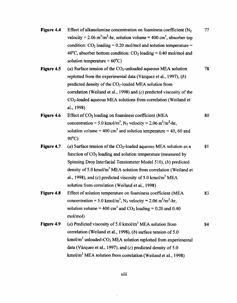
Figure 4.4 Effect of alkanolamine concentration on foaminess coefficient (N2 77
velocity = 2.06 m3/m2-hr, solution volume = 400 cm3, absorber top
condition: CO2 loading = 0.20 mol/mol and solution temperature =
40°C, absorber bottom condition: CO2 loading = 0.40 mol/mol and
solution temperature = 60°C)
Figure 4.5 (a) Surface tension of the CO2-unloaded aqueous MEA solution 78
replotted from the experimental data (Vazquez et al., 1997), (b)
predicted density of the CO2-loaded MEA solution from
correlation (Weiland et al., 1998) and (c) predicted viscosity of the
CO2-loaded aqueous MEA solutions from correlation (Weiland et
al., 1998)
Figure 4.6 Effect of CO2 loading on foaminess coefficient (MEA 80
concentration = 5.0 kmol/m3, N2 velocity = 2.06 m3/m2-hr,
solution volume = 400 cm3 and solution temperature = 40, 60 and
90°C)
Figure 4.7 (a) Surface tension of the CO2-loaded aqueous MEA solution as a 81
function of CO2 loading and solution temperature (measured by
Spinning Drop Interfacial Tensiometer Model 510), (b) predicted
density of 5.0 kmol/m3 MEA solution from correlation (Weiland et
al., 1998), and (c) predicted viscosity of 5.0 kmol/m3 MEA
solution from correlation (Weiland et al., 1998)
Figure 4.8 Effect of solution temperature on foaminess coefficient (MEA 83
concentration = 5.0 kmol/m3, N2 velocity = 2.06 m3/m2-hr,
solution volume = 400 cm3 and CO2 loading = 0.20 and 0.40
mol/mol)
Figure 4.9 (a) Predicted viscosity of 5.0 kmol/m3 MEA solution from 84
correlation (Weiland et al., 1998), (b) surface tension of 5.0
kmol/m3 unloaded-CO2 MEA solution replotted from experimental
data (Vazquez et al., 1997), and (c) predicted density of 5.0
kmol/m3 MEA solution from correlation (Weiland et al., 1998)
Figure 4.4 Effect of alkanolamine concentration on foaminess coefficient (N2 77
velocity = 2.06 m3/m2-hr, solution volume = 400 cm3, absorber top
condition: CO2 loading = 0.20 mol/mol and solution temperature =
40°C, absorber bottom condition: CO2 loading = 0.40 mol/mol and
solution temperature = 60°C)
Figure 4.5 (a) Surface tension of the C02-unloaded aqueous ME A solution 78
replotted from the experimental data (Vazquez et al., 1997), (b)
predicted density of the CC>2-loaded MEA solution from
correlation (Weiland et al., 1998) and (c) predicted viscosity of the
CC>2-loaded aqueous MEA solutions from correlation (Weiland et
al., 1998)
Figure 4.6 Effect of CO2 loading on foaminess coefficient (MEA 80
concentration =5.0 kmol/m3, N2 velocity = 2.06 m3/m2-hr,
solution volume = 400 cm3 and solution temperature = 40, 60 and
90°C)
Figure 4.7 ( a ) Surface tension of the CC^-loaded aqueous MEA solution as a 81
function of CO2 loading and solution temperature (measured by
Spinning Drop Interfacial Tensiometer Model 510), (b) predicted
density of 5.0 kmol/m3 MEA solution from correlation (Weiland et
al., 1998), and (c) predicted viscosity of 5.0 kmol/m3 MEA
solution from correlation (Weiland et al., 1998)
Figure 4.8 Effect of solution temperature on foaminess coefficient (MEA 83
concentration = 5.0 kmol/m3, N2 velocity = 2.06 m3/m2-hr,
solution volume = 400 cm3 and CO2 loading = 0.20 and 0.40
mol/mol)
Figure 4.9 (a) Predicted viscosity of 5.0 kmol/m3 MEA solution from 84
correlation (Weiland et al., 1998), (b) surface tension of 5.0
kmol/m3 unloaded-C02 MEA solution replotted from experimental
data (Vazquez et al., 1997), and (c) predicted density of 5.0
kmol/m3 MEA solution from correlation (Weiland et al., 1998)
xiii

Figure 4.10 Effect of corrosion inhibitors on foaminess coefficient (corrosion 88
inhibitor = NaVO3, CuCO3 and Na2SO3, corrosion inhibitor
concentration = 1000 ppm, MEA concentration = 5.0 kmol/m3, N2
velocity = 2.06 m3/m2-hr, solution volume = 400 cm3, CO2 loading
= 0.40 mol/mol and solution temperature = 60°C)
Figure 4.11 (a) Surface tension of the CO2-unloaded aqueous alkanolamine 93
solution as a function of alkanolamine concentration (40°C)
replotted from experimental data (Vazquez et al., 1996 and 1997
and Alvarez et al., 1998), (b) density of the CO2-unloaded aqueous
alkanolamine solution as a function of alkanolamine concentration
(60°C) replotted from experimental data (Maham et al., 1994;
Maham et al., 1995 and Henni et al., 2003), and (c) viscosity of the
CO2-unloaded aqueous alkanolamine solution as a function of
alkanolamine concentration (60°C) replotted from experimental
data (Teng et al., 1994; Maham et al., 2002 and Henni et al., 2003)
Figure 4.12 (a) Surface tension of CO2-unloaded aqueous blended 94
alkanolamine solutions at 60°C replotted from experimental data:
MEA+MDEA (Alvarez et al., 1998), DEA+MDEA (Alvarez et al.,
1998) and MEA+AMP (Vazquez et al., 1997), (b) predicted
viscosity of CO2-unloaded aqueous blended alkanolamine solution
with 4.0 kmol/m3 total concentration at 60°C (Mandal et al., 2003)
Figure 5.1 Framework of the foam height correlation 98
Figure 5.2 Schematic diagram of the pressures exerted on the gas bubble in 105
the liquid solution
Figure 5.3 Example of the foam observed in the static foaming experiment 106
Figure 5.4 Parity chart between H„p and H for the foam height correlation 113
(dashed•lines represent 95% confidence interval)
Figure 5.5 Simulation results of predicted foam height with respect to 116
superficial gas velocity (solution volume = 400 cm3, CO2 loading
= 0.40 mol/mol and solution temperature = 40°C) with MEA
concentration (a) 2.0 kmol/m3 and (b) 5.0 kmol/m3
xiv
Figure 4.10 Effect of corrosion inhibitors on foaminess coefficient (corrosion 88
inhibitor = NaVC>3, CUCO3 and Na2S03, corrosion inhibitor
concentration = 1000 ppm, MEA concentration = 5.0 kmol/m3, N2
velocity = 2.06 m3/m2-hr, solution volume = 400 cm3, CO2 loading
= 0.40 mol/mol and solution temperature = 60°C)
Figure 4.11 (a ) Surface tension of the C02-unloaded aqueous alkanolamine 93
solution as a function of alkanolamine concentration (40°C)
replotted from experimental data (Vazquez et al., 1996 and 1997
and Alvarez et al., 1998), (b) density of the C02-unloaded aqueous
alkanolamine solution as a function of alkanolamine concentration
(60°C) replotted from experimental data (Maham et al., 1994;
Maham et al., 1995 and Henni et al., 2003), and (c) viscosity of the
C02-unloaded aqueous alkanolamine solution as a function of
alkanolamine concentration (60°C) replotted from experimental
data (Teng et al., 1994; Maham et al., 2002 and Henni et al., 2003)
Figure 4.12 (a) Surface tension of CCh-unloaded aqueous blended 94
alkanolamine solutions at 60°C replotted from experimental data:
MEA+MDEA (Alvarez et al., 1998), DEA+MDEA (Alvarez et al.,
1998) and MEA+AMP (Vazquez et al., 1997), (b) predicted
viscosity of CCVunloaded aqueous blended alkanolamine solution
with 4.0 kmol/m3 total concentration at 60°C (Mandal et al., 2003)
Figure 5.1 Framework of the foam height correlation 98
Figure 5.2 Schematic diagram of the pressures exerted on the gas bubble in 105
the liquid solution
Figure 5.3 Example of the foam observed in the static foaming experiment 106
Figure 5.4 Parity chart between Hexp and H for the foam height correlation 113
(dashed'lines represent 95% confidence interval)
Figure 5.5 Simulation results of predicted foam height with respect to 116
superficial gas velocity (solution volume = 400 cm3, CO2 loading
= 0.40 mol/mol and solution temperature = 40°C) with MEA
concentration (a) 2.0 kmol/m3 and (b) 5.0 kmol/m3
xiv

Figure 5.6 Simulation results of predicted foam height with respect to 117
solution volume (MEA concentration = 2.0 kmol/m3, superficial
gas velocity = 0.57 mm/s, CO2 loading = 0.40 mol/mol and
solution temperature = 40°C)
Figure 5.7 Simulation results of predicted foam height with respect to MEA 118
concentration (superficial gas velocity = 0.57 mm/s and solution
volume = 400 cm3); (a) absorber top condition: CO2 loading =
0.20 mol/mol and solution temperature = 40°C and (b) absorber
bottom condition: CO2 loading = 0.40 mol/mol and solution
temperature = 60°C
Figure 5.8 Simulation results of predicted foam height with respect to CO2 119
loading (MEA concentration = 5.0 kmol/m3, superficial gas
velocity = 0.57 mm/s and solution volume = 400 cm3) with
solution temperature (a) 40°C, (b) 60°C, and (c) 90°C
Figure 5.9 Simulation results of predicted foam height with respect to 120
solution temperature (MEA concentration = 5.0 kmol/m3,
superficial gas velocity = 0.57 mm/s and solution volume = 400
cm3) with CO2 loading (a) 0.20 mol/mol and (b) 0.40 mol/mol
Figure 5.10 Sensitivity analysis of process parameters on foam height; (a) 127
minimum value of the remaining process parameters and (b)
maximum value of the remaining process parameters
Figure 5.11 Sensitivity analysis of physical properties on foam height; (a) 128
minimum value of the remaining process parameters and (b)
maximum value of the remaining process parameters
Figure 6.1 Concept of a foam model development 131
Figure 6.2 Model framework to predict total foam volume in a structured 132
packed absorber
X V
Figure 5.6 Simulation results of predicted foam height with respect to 117
solution volume (MEA concentration = 2.0 kmol/m3, superficial
gas velocity = 0.57 mm/s, CO2 loading = 0.40 mol/mol and
solution temperature = 40°C)
Figure 5.7 Simulation results of predicted foam height with respect to MEA 118
concentration (superficial gas velocity = 0.57 mm/s and solution
volume = 400 cm3); (a) absorber top condition: CO2 loading =
0.20 mol/mol and solution temperature = 40°C and (b) absorber
bottom condition: CO2 loading = 0.40 mol/mol and solution
temperature = 60°C
Figure 5.8 Simulation results of predicted foam height with respect to CO2 119
loading (MEA concentration = 5.0 kmol/m3, superficial gas
velocity = 0.57 mm/s and solution volume = 400 cm3) with
solution temperature (a) 40°C, (b) 60°C, and (c) 90°C
Figure 5.9 Simulation results of predicted foam height with respect to 120
solution temperature (MEA concentration = 5.0 kmol/m3,
superficial gas velocity = 0.57 mm/s and solution volume = 400
cm3) with CO2 loading (a) 0.20 mol/mol and (b) 0.40 mol/mol
Figure 5.10 Sensitivity analysis of process parameters on foam height; (a) 127
minimum value of the remaining process parameters and (b)
maximum value of the remaining process parameters
Figure 5.11 Sensitivity analysis of physical properties on foam height; (a) 128
minimum value of the remaining process parameters and (b)
maximum value of the remaining process parameters
Figure 6.1 Concept of a foam model development 131
Figure 6.2 Model framework to predict total foam volume in a structured 132
packed absorber
xv

Figure 6.3 (a) An arrangement of corrugated sheets with flow directions of 134
gas and liquid, (b) a location of foam layer on a surface of a
corrugated sheet with a certain crimp dimension and (c) a
mechanism of foam formation on a surface area of a packing
element
Figure 6.4 Illustration of four main forces affecting average bubble radius 139
Figure 6.5 (a) Experimental percent foam volume per packing volume plotted 143
versus the superficial gas velocity at different superficial liquid
velocities (MEA concentration = 5.0 kmol/m3, CO2 loading = 0.40
mol/mol, and solution temperature = 18.5°C) and (b) experimental
foam volume per packing volume plotted versus the L/G ratio
(MEA concentration = 5.0 kmol/m3, CO2 loading = 0.40 mol/mol,
and solution temperature = 18.5°C)
Figure 6.6 Example of turbulence developed at the bottom of the column 144
(superficial liquid velocity = 2.3 m3/m2-hr and superficial gas
velocity = 360 mm/s)
Figure 6.7 Simulation results compared between the experimental and 146
predicted percent foam volume per packing volume
Figure 6.8 Simulated profiles of local foam volumes along the absorber 148
height under various CO2 absorption conditions: (a) effect of CO2
loading of feed solution at three different superficial liquid
velocities (feed solution temperature = 33.2 ± 1.1°C, air flow rate
= 38.5 kmol/m2-hr and MEA concentration = 3.0 kmol/m3) and (b)
effect of the temperature of feed solution at three different
superficial liquid velocities (CO2 loading of feed solution = 0.33
mol/mol, air flow rate = 38.5 kmol/m2-hr, and MEA concentration
= 3.0 kmol/m3)
xvi
Figure 6.3 (a) An arrangement of corrugated sheets with flow directions of 134
gas and liquid, (b) a location of foam layer on a surface of a
corrugated sheet with a certain crimp dimension and (c) a
mechanism of foam formation on a surface area of a packing
element
Figure 6.4 Illustration of four main forces affecting average bubble radius 139
Figure 6.5 (a) Experimental percent foam volume per packing volume plotted 143
versus the superficial gas velocity at different superficial liquid
velocities (MEA concentration = 5.0 kmol/m3, CO2 loading = 0.40
mol/mol, and solution temperature = 18.5°C) and (b) experimental
foam volume per packing volume plotted versus the LIG ratio
(MEA concentration = 5.0 kmol/m3, CO2 loading = 0.40 mol/mol,
and solution temperature = 18.5°C)
Figure 6.6 Example of turbulence developed at the bottom of the column 144
(superficial liquid velocity = 2.3 m3/m2-hr and superficial gas
velocity = 360 mm/s)
Figure 6.7 Simulation results compared between the experimental and 146
predicted percent foam volume per packing volume
Figure 6.8 Simulated profiles of local foam volumes along the absorber 148
height under various CO2 absorption conditions: (a) effect of CO2
loading of feed solution at three different superficial liquid
velocities (feed solution temperature = 33.2 ± 1.1°C, air flow rate
= 3 8 . 5 k m o l / m 2 - h r a n d M E A c o n c e n t r a t i o n = 3 . 0 k m o l / m 3 ) a n d ( b )
effect of the temperature of feed solution at three different
superficial liquid velocities (CO2 loading of feed solution = 0.33
mol/mol, air flow rate = 38.5 kmol/m2-hr, and MEA concentration
= 3.0 kmol/m3)
xvi

Figure 6.9 Effect of the degradation product (ammonium thiosulfate) and 150
corrosion inhibitor (sodium metavanadate) on the simulated
foaming profile along the absorber (air flow rate = 38.5 kmol/m2-
hr, MEA concentration = 3.0 kmol/m3, CO2 loading of feed
solution = 0.33 mol/mol, superficial liquid velocity = 12.2 m3/m2-
hr, and feed solution temperature = 21.1°C (Aroonwilas, 2001)
Figure 6.10 Effect of the foaming on the gas volumetric flow rate for non- 153
degraded and degraded MEA solutions containing degradation
product (ammonium thiosulfate) and corrosion inhibitor (sodium
metavanadate) (MEA concentration = 3.0 kmol/m3, lean and rich
CO2 loading of the solution = 0.20 and 0.55 mol/mol, respectively,
feed solution temperature = 40°C, and CO2 concentration in the
gas phase = 15%)
xvii

Nomenclature
a1,...,a6 coefficients used in Subroutine 3
constant between interaction energy of molecular pair ij
an exponent of physical variable of n
ap specific surface area of packing material (m2/m3 packing)
A cross-sectional area
As surface area (m2)
b slab width (m)
b1,...,b6 coefficients used in Subroutine 3
bh constant for Equation (2.19)
B half of corrugation base width (m)
c constant for Equation (6.12)
ci,..•,c6 coefficients used in Subroutine 3
Ca capillary number
d bubble diameter (mm)
dave average bubble diameter (m)
d, diameter of bubble entering the foam layer (m)
dx, dy, dz increment of distance in the x-, y- and z-axis, respectively
Dc column diameter (m)
Dh diameter of perforation hole (mm)
E surface elasticity (mN/m)
E eff effective elasticity (mN/m)
EM Marangoni dilational modulus (mN/rn)
xviii
Nomenclature
ai,...,a6 coefficients used in Subroutine 3
ay constant between interaction energy of molecular pair ij
a„ exponent of physical variable of n
ap specific surface area of packing material (m2/m3 packing)
^ cross-sectional area
As surface area (m2)
b slab width (m)
bj,...,b(5 coefficients used in Subroutine 3
bh constant for Equation (2.19)
B half of corrugation base width (m)
c constant for Equation (6.12)
ci,...,c6 coefficients used in Subroutine 3
Ca capillary number
d bubble diameter (mm)
d^e average bubble diameter (m)
d„ diameter of bubble entering the foam layer (m)
dx, dy, dz increment of distance in the x-, y- and z-axis, respectively
Dc column diameter (m)
Dh diameter of perforation hole (mm)
E surface elasticity (mN/m)
Eeff effective elasticity (mN/m)
EM Marangoni dilational modulus (mN/m)
xviii

fpe,foration perforation factor of the packing element
fweited fraction of the wetted surface area
F8 buoyancy force
Fy hydrostatic force
FK kinetic force
Fs surface tension force
Fr Froude number
g gravitational acceleration (m/s2)
G Gibbs free energy (J)
Gexcess molar excess Gibbs free energy (J)
Gidea! molar Gibbs free energy of the ideal solution (J)
G gas flow rate (m3/s)
G gas flow rate per unit area or superficial gas velocity
6, critical superficial gas velocity
Gm minimum superficial gas velocity (mm/s)
hcrimp crimp height
hd height of gas dispersion layer (m)
hiiq liquid height above the perforation hole (m)
hp height of packing element (m)
h' liquid holdup (m3 liquid solution/m3 packing)
H pneumatic steady-state foam height
Hexp experimental steady-state foam height
the number of dimensional parameters
xix
/perforation
fwetted
Fb
FH
FK
Fs
Fr
8
G
Gexcess
G ideal
G
G
GL
hcrimp
hd
hliq
hp
h'
H
exp
perforation factor of the packing element
fraction of the wetted surface area
buoyancy force
hydrostatic force
kinetic force
surface tension force
Froude number
gravitational acceleration (m/s )
Gibbs free energy (J)
molar excess Gibbs free energy (J)
molar Gibbs free energy of the ideal solution (J)
gas flow rate (m3/s)
gas flow rate per unit area or superficial gas velocity
critical superficial gas velocity
minimum superficial gas velocity (mm/s)
crimp height
height of gas dispersion layer (m)
liquid height above the perforation hole (m)
height of packing element (m)
liquid holdup (m3 liquid solution/m3 packing)
pneumatic steady-state foam height
experimental steady-state foam height
the number of dimensional parameters
xix

k
K
Kf
Ki,
1
L/G
L
m,
M
MW,
n
N
N bub
NT
P
PC
P H,d
P Hi
P inside
P outside
P.
gdown
the total number of fundamental units needed to express the
system
adjustable parameter for Equation (2.16)
constant for Equation (2.21)
constant for Equation (2.20)
capillary perimeter (mm)
liquid-to-gas ratio (kg solution/kg air)
liquid flow rate per unit area or superficial liquid velocity
mass percent of i
MEA concentration (kmol/m3)
molecular weight of i
the number of physical variables
adjustable parameter for Equation (2.16)
the number of bubbles formed at diffuser per unit of time
the total number of slabs per a packing section of interest
operating pressure (N/m2)
capillary pressure (N/m2)
hydrostatic pressure due to gas dispersion layer (N/m2)
hydrostatic pressure due to foam layer (N/m2)
pressure inside of the gas bubble (N/m2)
pressure outside of the gas bubble (N/m2)
additional pressure term (N/m2)
rate of liquid in lamella flowing back to the bulk solution (m/s)
XX
k the total number of fundamental units needed to express
system
K adjustable parameter for Equation (2.16)
KJ constant for Equation (2.21)
KP constant for Equation (2.20)
I capillary perimeter (mm)
L/G liquid-to-gas ratio (kg solution/kg air)
L liquid flow rate per unit area or superficial liquid velocity
NTI mass percent of i
M MEA concentration (kmol/m3)
MW, molecular weight of i
n the number of physical variables
N adjustable parameter for Equation (2.16)
Nbub the number of bubbles formed at diffuser per unit of time
Nt the total number of slabs per a packing section of interest
P operating pressure (N/m2)
Pc capillary pressure (N/m2)
PHJ hydrostatic pressure due to gas dispersion layer (N/m2)
PHJ hydrostatic pressure due to foam layer (N/m2)
P inside pressure inside of the gas bubble (N/m2)
P outside pressure outside of the gas bubble (N/m2)
P* additional pressure term (N/m2)
(Jdown rate of liquid in lamella flowing back to the bulk solution (m/s)
XX

• film rate of liquid from the bulk solution moving upward to the foam
layer through the foam films (m/s)
q,, PB rate of liquid from the bulk solution moving upward to the foam
layer through the Plateau borders (m/s)
Qn physical variable of n
r average bubble radius (mm)
reg effective average radius of bubble
r 1,,prechcted average bubble radius predicted using the Laplace equation
R universal gas constant
RI, R2 principal radii of curvature (mm)
Re Reynolds number
s the number of immobile surfaces
S, additional physical variable of i
Sr sum of squares of residuals
T temperature
u velocity of liquid in the vertical lamella (rnm/s)
U„ interaction energy of molecular pair ii
interaction energy of molecular pair ij
U,, interaction energy of molecular pair jj
v, molar volume of pure component i at constant temperature
molar volume of pure component j at constant temperature
molar volume of i (ml/mol)
Vbub bubble volume (m3)
Vso1 solution volume (cm3) xxi
gup, film rate of liquid from the bulk solution moving upward to the foam
layer through the foam films (m/s)
qup PB rate of liquid from the bulk solution moving upward to the foam
layer through the Plateau borders (m/s)
Q„ physical variable of n
r average bubble radius (mm)
reff effective average radius of bubble
j/,predicted average bubble radius predicted using the Laplace equation
R universal gas constant
Ri, R2 principal radii of curvature (mm)
Re Reynolds number
5 the number of immobile surfaces
Si additional physical variable of i
Sr sum of squares of residuals
T temperature
u velocity of liquid in the vertical lamella (mm/s)
Uu interaction energy of molecular pair ii
U,j interaction energy of molecular pair ij
Ujj interaction energy of molecular pair jj
Vi molar volume of pure component i at constant temperature
Vj molar volume of pure component j at constant temperature
V, molar volume of i (ml/mol)
Vbub bubble volume (m3)
Vsoi solution volume (cm3) xxi

Vy constant for Equation (5.15)
V** molar volume due to the interaction between MEA and CO2
Vr" liquid volume after supplying gas to the test cell (cm3)
Ve entire gas volume dispersed through the diffuser (m3)
w constant for Equation (6.12)
x, mole fraction of i
Greek letter
a corrugation angle (°)
aco2 CO2 loading (mol CO2/mol MEA)
y surface tension
Yslag slag surface tension (N/m)
Ay surface tension gradient (mN/m)
g film thickness
acr critical thickness of the lamella film (m)
Save average gas fraction in the foam layer
sd gas fraction in the gas dispersion layer
sf gas fraction in the foam layer
acute angle of a slab with respect to the next corrugation sheet
A parameter defined by Equation (5.21)
viscosity
slag viscosity (Pa.$)
V'
V"
•ycell
ygff
w
Xi
Greek letter
a
aco2
r
Yslag
Ay
S
dCr
Save
ed
*
9
A
H
Mslag
constant for Equation (5.15)
molar volume due to the interaction between MEA and CO2
liquid volume after supplying gas to the test cell (cm3)
entire gas volume dispersed through the diffuser (m )
constant for Equation (6.12)
mole fraction of i
corrugation angle (°)
CO2 loading (mol CCVmol MEA)
surface tension
slag surface tension (N/m)
surface tension gradient (mN/m)
film thickness
critical thickness of the lamella film (m)
average gas fraction in the foam layer
gas fraction in the gas dispersion layer
gas fraction in the foam layer
acute angle of a slab with respect to the next corrugation sheet
parameter defined by Equation (5.21)
viscosity
slag viscosity (Pa.s)
xxii

17i
p
Pstag
Op
Tbo
V
Vexp
Vslab
dimensionless parameter of i
density (kg/m3)
slag density (kg/m3)
difference between liquid and gas density (kg/m3)
foaminess coefficient
binary coalescence time (s)
average steady-state foam volume (m3)
experimental steady-state foam volume (cm3)
slap foam volume (m3)
total foam volume (m3)
Subscript
CO2 carbon dioxide
G gas
1120 water
L liquid
MEA monoethanolamine
N2 nitrogen
Abbreviation
AAD average absolute deviation
AMP 2-amino-2-methyl-l-propanol
DEA diethanolamine
nt
p
pslag
Ap
E
T-bo
V
Vexp
Vslab
or
Subscript
co2
G
H20
L
MEA
N2
Abbreviation
AAD
AMP
DEA
dimensionless parameter of i
density (kg/m3)
slag density (kg/m3)
difference between liquid and gas density (kg/m )
foaminess coefficient
binary coalescence time (s)
average steady-state foam volume (m3)
experimental steady-state foam volume (cm3)
•5
slap foam volume (m )
total foam volume (m3)
carbon dioxide
gas
water
liquid
monoethanolamine
nitrogen
average absolute deviation
2-amino-2-methyl-1 -propanol
diethanolamine
xxiii

DEP 1-(2-hydroxyethyl) piperazine
DGA diglycolamine
DIPA diisopropanolamine
HEP 1,4-Bis (2-hydroxyethyl)piperazine
MDEA N-methyldiethanolamine
MEA monoethanolamine
MMSCFD million standard cubic feet per day
PB Plateau border
PM particulate matter
PZ piperazine
R&D research and development
scfm standard cubic foot per minute
SDBS sodium dodecylbenzene sulphonate
xxiv
DEP l-(2-hydroxyethyl) piperazine
DGA diglycolamine
DIPA diisopropanolamine
HEP 1,4-Bis (2-hydroxyethyl)piperazine
MDEA N -methy Idiethanolamine
MEA monoethanolamine
MMSCFD million standard cubic feet per day
PB Plateau border
PM particulate matter
PZ piperazine
R&D research and development
scfm standard cubic foot per minute
SDBS sodium dodecylbenzene sulphonate
xxiv

1. INTRODUCTION
Coal-fired power plants generate electricity by combusting coal to produce high
pressure steam, which drives a series of turbines and generators. The coal combustion
produces flue gas containing a number of air pollutants currently being regulated or to be
regulated in the near future under various environmental laws. These pollutants include
hazardous pollutants such as mercury (Hg) and also criteria pollutants such as particulate
matter (PM), sulfur oxides (SOX), and nitrogen oxides (N0x). The coal-fired power plants
also produce and release carbon dioxide (CO2), a major greenhouse gas contributing to
global climate change, to the atmosphere. The CO2 emission is of great concern due to its
large quantity and implications to the environment. It is predicted that coal combustion
will contribute approximately 45 percent of the total world CO2 emissions (40385 million
metric tonnes) in 2030. The coal combustion from the United States and Canada is
predicted to contribute about 15.9 and 1.8 percent, respectively, of the world CO2
emissions in 2030 (EIA, 2009).
To enforce the reduction of global greenhouse gas emissions, delegates from
many countries attending the United Nations climate change conference held in
December 2009 in Copenhagen have agreed on the Copenhagen Accord (UNFCCC,
2009a). Under this accord, Canada recently submitted an emissions target of 17 percent
reduction from 2005's level by 2020 to the United Nations Framework Convention on
Climate Change (UNFCCC, 2009b). One of the reduction strategies to help Canada and
other nations achieve their target is to capture CO2 from combustion flue gas streams
generated by coal-fired power plants since CO2 emission from these power stations is
expected to contribute about 60 percent of the total world CO2 emissions that are released
1. INTRODUCTION
Coal-fired power plants generate electricity by combusting coal to produce high
pressure steam, which drives a series of turbines and generators. The coal combustion
produces flue gas containing a number of air pollutants currently being regulated or to be
regulated in the near future under various environmental laws. These pollutants include
hazardous pollutants such as mercury (Hg) and also criteria pollutants such as particulate
matter (PM), sulfur oxides (SOx), and nitrogen oxides (NOx). The coal-fired power plants
also produce and release carbon dioxide (CO2), a major greenhouse gas contributing to
global climate change, to the atmosphere. The CO2 emission is of great concern due to its
large quantity and implications to the environment. It is predicted that coal combustion
will contribute approximately 45 percent of the total world CO2 emissions (40385 million
metric tonnes) in 2030. The coal combustion from the United States and Canada is
predicted to contribute about 15.9 and 1.8 percent, respectively, of the world CO2
emissions in 2030 (EIA, 2009).
To enforce the reduction of global greenhouse gas emissions, delegates from
many countries attending the United Nations climate change conference held in
December 2009 in Copenhagen have agreed on the Copenhagen Accord (UNFCCC,
2009a). Under this accord, Canada recently submitted an emissions target of 17 percent
reduction from 2005's level by 2020 to the United Nations Framework Convention on
Climate Change (UNFCCC, 2009b). One of the reduction strategies to help Canada and
other nations achieve their target is to capture CO2 from combustion flue gas streams
generated by coal-fired power plants since CO2 emission from these power stations is
expected to contribute about 60 percent of the total world CO2 emissions that are released

by large stationary point sources using combustion of fossil fuels (Metz et al., 2005).
This strategy also enables the continuation of fossil fuel utilization to meet energy
demand as alternative energy sources are developed. The CO2 capture unit can be
integrated into the power plant as a flue gas post-treatment unit with the arrangement
shown in Figure 1.1. This is to treat the flue gas after the removal of PM and SO2 in order
to prevent plugging and fouling and to minimize degradation of CO2 capture solvents.
Although CO2 capture can be technically implemented by a number of gas
separation methods, gas absorption into a liquid solvent is the most attractive because of
its maturity in gas treating services. For many decades, the alkanolamine-based gas
absorption process has played a significant role in gas sweetening plants in removing
acid gases from gas streams. This process is currently gaining a great deal of interest as
an environmental abatement unit for capturing CO2 from industrial flue gas streams
generated by coal-fired power plants. The existing power plants that are integrated with
the alkanolamine absorption-based CO2 capture unit are listed in Table 1.1. Most of these
CO2 capture units are R&D scale pilot plants in which the feed gas is a slipstream of flue
gas produced by a power plant.
2
by large stationary point sources using combustion of fossil fuels (Metz et al., 2005).
This strategy also enables the continuation of fossil fuel utilization to meet energy
demand as alternative energy sources are developed. The CO2 capture unit can be
integrated into the power plant as a flue gas post-treatment unit with the arrangement
shown in Figure 1.1. This is to treat the flue gas after the removal of PM and SO2 in order
to prevent plugging and fouling and to minimize degradation of CO2 capture solvents.
Although CO2 capture can be technically implemented by a number of gas
separation methods, gas absorption into a liquid solvent is the most attractive because of
its maturity in gas treating services. For many decades, the alkanolamine-based gas
absorption process has played a significant role in gas sweetening plants in removing
acid gases from gas streams. This process is currently gaining a great deal of interest as
an environmental abatement unit for capturing CO2 from industrial flue gas streams
generated by coal-fired power plants. The existing power plants that are integrated with
the alkanolamine absorption-based CO2 capture unit are listed in Table 1.1. Most of these
C02 capture units are R&D scale pilot plants in which the feed gas is a slipstream of flue
gas produced by a power plant.
2

Electricity supply to community
COAL-FIRED POWER PLANT
CO2 for utilization and storage
FLUE GAS TREATMENT
Flue gas M
Emit to atmosphere
Figure 1.1 Schematic diagram of a coal-fired power plant with post-combustion
treatment processes
3
Electricity supply to community
C02 for utilization and storage
Emit to atmosphere
FLUE GAS TREATMENT
COAL-FIRED POWER PLANT
Flue gas PM S02
Figure 1.1 Schematic diagram of a coal-fired power plant with post-combustion
treatment processes
3

Table 1.1 List of examples of coal-fired power plants with an alkanolamine-based CO2
absorption process as a CO2 capture unit
Power plant Type of Plant CO2 capacity Use of Reference coal capacity (Tonne CO2 CO2
(MW) /day)
Warrior Run power station (Cumberland,
Bituminous coal
229 150 Food industry
Davison et al., 2001
USA)
Boundary Dam power station (Saskatchewan,
Lignite coal 813 up to 4 CO2product
Idem et al., 2006
Canada)
Esbjerg power station (Esbjerg, Denmark)
400 24 CO2product
Knudsen et al., 2009
Niederaussem power station (Niederaussem,
Lignite coal 3864 Up to 7.2 CO2product
Moser et al., 2009
Germany)
4
Table 1.1 List of examples of coal-fired power plants with an alkanolamine-based CO2
absorption process as a CO2 capture unit
Power plant Type of coal
Plant capacity (MW)
C02 capacity (Tonne C02
/day)
Use of co2
Reference
Warrior Run power station (Cumberland, USA)
Bituminous coal
229 150 Food industry
Davison et al., 2001
Boundary Dam power station (Saskatchewan, Canada)
Lignite coal 813 up to 4 C02
product Idem et al., 2006
Esbjerg power station (Esbjerg, Denmark)
- 400 24 C02
product Knudsen et al., 2009
Niederaussem power station (Niederaussem, Germany)
Lignite coal 3864 Up to 7.2 C02
product Moser et al., 2009
4

1.1 Process description of regenerable CO2 absorption
Figure 1.2 illustrates a typical configuration of the CO2 absorption process using a
regenerable liquid solvent. The process consists of two major sections, an absorption
section where CO2 in the flue gas is absorbed into the liquid solvent and a regeneration
section where the absorbed CO2 is stripped out by means of heat. In the absorption
section, the gas stream containing CO2 is passed upward through the absorber,
countercurrent to the solvent entering the absorber at the top. Under proper conditions,
CO2 is transferred from the gas stream to the liquid solvent, resulting in a treated gas with
low CO2 content passing out of the absorber top and a CO2-rich solvent leaving the
absorber at the bottom. The rich solvent is then heated in a lean/rich heat exchanger and
enters the regenerator at some point near the top. The CO2-rich solvent is heated to
boiling in the regeneration section by a hot steam reboiler located at the bottom of the
regenerator. The captured CO2 is thereby released from the solvent. Finally, the CO2-lean
solvent is pumped from the regenerator through the lean/rich heat exchanger and a cooler
before being re-introduced to the absorber.
It is recognized that the chemical solvents for CO2 capture are subject to
degradation problems characterized an accumulation of non-regenerable and inactive
products during the process. A reclaimer attached to the hot steam reboiler is used
periodically to remove such degradation products, particularly when the level of these
products exceeds certain amounts (e.g., 1.2 wt% heat stable salt anion of solution (CCR
technologies, 2006) or 10 wt% heat stable salt of total alkanolamine concentration
(DuPart et al., 1993)). An inline filtration is also used in parallel to remove some
degradation products. Makeup tanks for water and alkanolamine solutions are in use for
5
1.1 Process description of regenerable CO2 absorption
Figure 1.2 illustrates a typical configuration of the CO2 absorption process using a
regenerable liquid solvent. The process consists of two major sections, an absorption
section where CO2 in the flue gas is absorbed into the liquid solvent and a regeneration
section where the absorbed CO2 is stripped out by means of heat. In the absorption
section, the gas stream containing CO2 is passed upward through the absorber,
countercurrent to the solvent entering the absorber at the top. Under proper conditions,
CO2 is transferred from the gas stream to the liquid solvent, resulting in a treated gas with
low CO2 content passing out of the absorber top and a C02-rich solvent leaving the
absorber at the bottom. The rich solvent is then heated in a lean/rich heat exchanger and
enters the regenerator at some point near the top. The CC>2-rich solvent is heated to
boiling in the regeneration section by a hot steam reboiler located at the bottom of the
regenerator. The captured CO2 is thereby released from the solvent. Finally, the C02-lean
solvent is pumped from the regenerator through the lean/rich heat exchanger and a cooler
before being re-introduced to the absorber.
It is recognized that the chemical solvents for CO2 capture are subject to
degradation problems characterized an accumulation of non-regenerable and inactive
products during the process. A reclaimer attached to the hot steam reboiler is used
periodically to remove such degradation products, particularly when the level of these
products exceeds certain amounts (e.g., 1.2 wt% heat stable salt anion of solution (CCR
technologies, 2006) or 10 wt% heat stable salt of total alkanolamine concentration
(DuPart et al., 1993)). An inline filtration is also used in parallel to remove some
degradation products. Makeup tanks for water and alkanolamine solutions are in use for
5

making up the solvent concentration due to degradation and solvent loss, thereby
maintaining the desired CO2 capture efficiency of the process.
6
making up the solvent concentration due to degradation and solvent loss, thereby
maintaining the desired CO2 capture efficiency of the process.
6

CO2 and steam
SOLVENT/WATER MAKEUP TANK
Treated gas 4 Lean
solution
ABSORBER
Flue gas
REGENERATOR
Rich Bplux solution
COOLER I Lean solution
LEAN LEAN/RICH SOLUTION
HEAT PUMP EXCHANGER
Rich solution
BOOSTER PUMP RECLAIMER Drain
OVERHEAD CONDENSER
CO2
1-- " )
REFLUX PUMP PUMP
REFLUX DRUM
Steaml v REBOILER
I Steam(
Figure 1.2 Schematic diagram of a typical absorption-based CO2 capture unit
7
C02 and steam OVERHEAD
CONDENSER
if _co2
REGENERATOR SOLVENT/WATER
MAKEUP TANK Rich solution
fteflux Treated gas
Lean solution
REFLUX DRUM
COOLEI Lean solution
REFLUX PUMP ABSORBER
LEAN SOLUTION
PUMP
LEAN/RICH ~ HEAT
EXCHANGER REBOILER
Flue gas.
Rich solution Steam
BOOSTER PUMP RECLAIMER Drain
Figure 1.2 Schematic diagram of a typical absorption-based CO2 capture unit
7

1.2 Process solution
1.2.1 Absorption solvent
At present, there are a number of absorption solvents commercially available for
CO2 capture. They are classified into two categories, chemical and physical solvents. The
chemical solvents are commonly used for treating gas streams with low- and moderate-
CO2 partial pressure while the physical solvents are suitable for high-pressure gas
streams. The typical chemical solvents are alkanolamines commonly used in forms of
aqueous solutions. These chemical solvents include monoethanolamine (MEA),
diethanolamine (DEA), N-methyldiethanolamine (MDEA), diglycolamine (DGA),
diisopropanolamine (DIPA), and 2-amino-2-methyl- 1 -propanol (AMP). Mixtures of
these single alkanolamines known as blended alkanolamines are also gaining a great deal
of interest from practitioners due to their process advantages over the single
alkanolamines. Common formulations of the blended alkanolamines are tertiary
alkanolamines, which are designed for specific CO2 capture targets and purposes. MDEA
is gaining recognition as the key component of the blended alkanolamines because of its
low energy requirements and high CO2 absorption capacity. Addition of a primary amine
MEA or secondary amine DEA into the MDEA solution helps enhance the rate of CO2
capture while maintaining the advantages of MDEA.
The physical solvents are commonly used for high-pressure gas streams. They
require less energy for solvent regeneration than the chemical solvents. Examples of the
physical solvents are propylene carbonate, Selexol, methanol, and N-methyl-2-
pyrrolidone. It is commonly known that the physical solvents alone are ineffective for
low-pressure gas streams. However, mixing between chemical and physical solvents
could provide some benefits for CO2 capture under low-pressure conditions. For instance,
8
1.2 Process solution
1.2.1 Absorption solvent
At present, there are a number of absorption solvents commercially available for
CO2 capture. They are classified into two categories, chemical and physical solvents. The
chemical solvents are commonly used for treating gas streams with low- and moderate-
CO2 partial pressure while the physical solvents are suitable for high-pressure gas
streams. The typical chemical solvents are alkanolamines commonly used in forms of
aqueous solutions. These chemical solvents include monoethanolamine (MEA),
diethanolamine (DEA), N-methyldiethanolamine (MDEA), diglycolamine (DGA),
diisopropanolamine (DIPA), and 2-amino-2-methyl-l-propanol (AMP). Mixtures of
these single alkanolamines known as blended alkanolamines are also gaining a great deal
of interest from practitioners due to their process advantages over the single
alkanolamines. Common formulations of the blended alkanolamines are tertiary
alkanolamines, which are designed for specific CO2 capture targets and purposes. MDEA
is gaining recognition as the key component of the blended alkanolamines because of its
low energy requirements and high CO2 absorption capacity. Addition of a primary amine
MEA or secondary amine DEA into the MDEA solution helps enhance the rate of CO2
capture while maintaining the advantages of MDEA.
The physical solvents are commonly used for high-pressure gas streams. They
require less energy for solvent regeneration than the chemical solvents. Examples of the
physical solvents are propylene carbonate, Selexol, methanol, and N-methyl-2-
pyrrolidone. It is commonly known that the physical solvents alone are ineffective for
low-pressure gas streams. However, mixing between chemical and physical solvents
could provide some benefits for CO2 capture under low-pressure conditions. For instance,
8

blends of physical and chemical solvents such as Sulfinol-D (Sulfolane and DIPA) and
Sulfinol-M (Sulfolane and MDEA) have been found to be effective for the removal of
CO2 and sulfur compounds from gas streams (Gupta et al., 2003). Sulfolane physically
absorbs the bulk of CO2 while both DIPA and MDEA (chemical solvents) work as the
reactive species for capture activities to completely purify gas streams. These mixed
solvents also help reduce corrosion problems.
Apart from the typical alkanolamines mentioned above, there are also a large
number of solvents currently proposed and being investigated. Some of them are
proprietary. The Kansai Electric Company and Mitsubishi Heavy Industries developed a
family of energy-efficient proprietary solvents namely KS-1 (Mimura et al., 1995). This
solvent has been commercialized to recover CO2 from i) the flue gases generated by
natural gas-fired and oil-fired boilers for general use of CO2 such as beverage and dry ice
in Japan and ii) the steam reformer flue gas for urea production in Malaysia and India
(Iijima, 2008). The CO2 capture plant in Japan has a capacity of 330 tonnes of CO2
captured/day and those in Malaysia and India have a capacity of 200 and 450 (x 2 units)
tonnes of CO2 captured/day, respectively (Iijima, 2008). In 2006, an attempt to use the
KS-1 solvent to capture CO2 from coal-fired flue gases was tested in the 2x500 MW
bituminous coal-fired power plant in Matsushima, Japan with a capacity of 10 tonnes of
CO2 captured/day (Kishimoto et al., 2009).
Many researchers have investigated the performance of hot potassium carbonate
(K2CO3) plus DEA as an absorption rate enhancer (Savage et al., 1980; Tseng et al.,
1988; Pohorecki and Kucharski, 1991). Recently, a group of researchers from the
University of Texas at Austin has been testing the performance of blends between K2CO3
and piperazine (PZ) (Cullinane and Rochelle, 2004). Although comparison results
9
blends of physical and chemical solvents such as Sulfinol-D (Sulfolane and DIPA) and
Sulfinol-M (Sulfolane and MDEA) have been found to be effective for the removal of
CO2 and sulfur compounds from gas streams (Gupta et al., 2003). Sulfolane physically
absorbs the bulk of CO2 while both DIPA and MDEA (chemical solvents) work as the
reactive species for capture activities to completely purify gas streams. These mixed
solvents also help reduce corrosion problems.
Apart from the typical alkanolamines mentioned above, there are also a large
number of solvents currently proposed and being investigated. Some of them are
proprietary. The Kansai Electric Company and Mitsubishi Heavy Industries developed a
family of energy-efficient proprietary solvents namely K.S-1 (Mimura et al., 1995). This
solvent has been commercialized to recover CO2 from /) the flue gases generated by
natural gas-fired and oil-fired boilers for general use of CO2 such as beverage and dry ice
in Japan and if) the steam reformer flue gas for urea production in Malaysia and India
(Iijima, 2008). The CO2 capture plant in Japan has a capacity of 330 tonnes of CO2
captured/day and those in Malaysia and India have a capacity of 200 and 450 (x 2 units)
tonnes of CO2 captured/day, respectively (Iijima, 2008). In 2006, an attempt to use the
KS-1 solvent to capture CO2 from coal-fired flue gases was tested in the 2x500 MW
bituminous coal-fired power plant in Matsushima, Japan with a capacity of 10 tonnes of
CO2 captured/day (Kishimoto et al., 2009).
Many researchers have investigated the performance of hot potassium carbonate
(K2CO3) plus DEA as an absorption rate enhancer (Savage et al., 1980; Tseng et al.,
1988; Pohorecki and Kucharski, 1991). Recently, a group of researchers from the
University of Texas at Austin has been testing the performance of blends between K2CO3
and piperazine (PZ) (Cullinane and Rochelle, 2004). Although comparison results
9

between an aqueous solution of PZ with K2CO3 and an aqueous MEA solution as an
absorption solvent for a post-combustion CO2 absorption process obtained from rigorous
thermodynamic models showed that the aqueous MEA solution thermodynamically and
economically outperforms the aqueous PZ/K2CO3 solution, a further investigation by a
model with greater accuracy in prediction of heat of reaction and heat of capacity was
recommended to be used in further testing of the solvent (Oexmann and Kather, 2009).
Ammonia has also been investigated for quite a while (Huang et al., 2002) and has
recently been used in the demonstration CO2 capture units to capture flue gases produced
by i) the 50-MW R.E. Burger power plant in Ohio, USA (McLarnon and Duncan, 2009)
and ii) the 1226-MW Pleasant Prairie Power Plant in Wisconsin, USA (Kozak et al.,
2009). The former has a capacity of 20 tonnes of CO2 captured/day and the latter has a
capacity of more than 35 tonnes of CO2 captured/day.
1.2.2 Other chemicals
In addition to the absorption solvents, the process solution also contains
degradation products and chemical additives such as corrosion inhibitors, antifoam
agents, oxygen scavengers, and salt neutralizers. The degradation products are essentially
formed by degradation reactions of the absorption solvents with other chemical
constituents in the process solution. They can be either regenerable or nonregenerable
under normal operating conditions of CO2 stripping (or solvent regeneration) depending
on the types of chemical constituents taking part in the reactions. The degradation
products caused by CO2 are mostly regenerable and, hence, are not of great concern
compared to the nonregenerable products. The nonregenerable degradation products,
mainly heat stable salts, are formed through the reactions of the absorption solvents with
10
between an aqueous solution of PZ with K2CO3 and an aqueous MEA solution as an
absorption solvent for a post-combustion CO2 absorption process obtained from rigorous
thermodynamic models showed that the aqueous MEA solution thermodynamically and
economically outperforms the aqueous PZ/K2CO3 solution, a further investigation by a
model with greater accuracy in prediction of heat of reaction and heat of capacity was
recommended to be used in further testing of the solvent (Oexmann and Kather, 2009).
Ammonia has also been investigated for quite a while (Huang et al., 2002) and has
recently been used in the demonstration CO2 capture units to capture flue gases produced
by t) the 50-MW R.E. Burger power plant in Ohio, USA (McLarnon and Duncan, 2009)
and ii) the 1226-MW Pleasant Prairie Power Plant in Wisconsin, USA (Kozak et al.,
2009). The former has a capacity of 20 tonnes of CO2 captured/day and the latter has a
capacity of more than 35 tonnes of CO2 captured/day.
1.2.2 Other chemicals
In addition to the absorption solvents, the process solution also contains
degradation products and chemical additives such as corrosion inhibitors, antifoam
agents, oxygen scavengers, and salt neutralizers. The degradation products are essentially
formed by degradation reactions of the absorption solvents with other chemical
constituents in the process solution. They can be either regenerable or nonregenerable
under normal operating conditions of CO2 stripping (or solvent regeneration) depending
on the types of chemical constituents taking part in the reactions. The degradation
products caused by CO2 are mostly regenerable and, hence, are not of great concern
compared to the nonregenerable products. The nonregenerable degradation products,
mainly heat stable salts, are formed through the reactions of the absorption solvents with
10

acids stronger than CO2, such as carboxylic acids. The carboxylic acids are usually
introduced to the capture process along with makeup water and feed gas streams or
generated within the process by undergoing chemical reactions with gaseous components
such as 0 2, CO, and SO2. For example, formic and oxalic acids can be generated by the
reactions of MEA with CO and 0 2 as shown below:
Degradation by CO (modified from Rooney et al., 1997):
H2NCH2CH2OH + H2O --> Ii3NCH2CH2OH + Off (1.1)
CO + OH" —> HCOO" (1.2)
H3NCH2CH2OH + HCOO" —> H2NCH2CH2OH2+-HCOO" (1.3)
where H2NCH2CH2OH, HC00", and H2NCH2CH2OH2+-HCOO" denote MEA,
anion, heat-stable formate salt of MEA, respectively.
Degradation by 0 2 (modified from McCullough and Nielsen, 1996):
formate
H2NCH2CH2OH +'A 0 2 H2NCH2CHO (cc-amino acetaldehyde) (1.4)
H2NCH2CHO +''A 0 2 --> H2NCH2COOH (glycine) (1.5)
H2NCH2COOH + 0 2 --> HOCH2COOH (glycolic acid) (1.6)
HOCH2COOH + 0 2 -4 HCOCOOH (glyoxylic acid) (1.7)
HCOCOOH + 0 2 —> HOCOCOOH (oxalic acid) (1.8)
where H2NCH2CHO, H2NCH2COOH, HOCH2COOH, HCOCOOH, and HOCOCOOH
are cc-amino acetaldehyde, glycine, glycolic acid, glyoxylic acid, and glyoxylic acid,
respectively. Concentrations of common heat stable salts found in gas treating plants are
listed in Table 1.2. The presence of heat stable salts in the process solution causes a
number of adverse effects, including a reduction in acid gas absorption capacity of
alkanolamine, an increase in solution viscosity, an increase in foaming tendency of the
11
acids stronger than CO2, such as carboxylic acids. The carboxylic acids are usually
introduced to the capture process along with makeup water and feed gas streams or
generated within the process by undergoing chemical reactions with gaseous components
such as O2, CO, and SO2. For example, formic and oxalic acids can be generated by the
reactions of MEA with CO and O2 as shown below:
Degradation bv CO (modified from Rooney et al., 1997):
H2NCH2CH2OH + H20 -> H3NCH2CH2OH + OH' (1.1)
CO + OH" -> HCOO" (1.2)
H3NCH2CH2OH + HCOO" -> H2NCH2CH2OH2+-HCOO' (1.3)
where H2NCH2CH2OH, HCOO", and H2NCH2CH2OH2+-HCOO- denote MEA, formate
anion, heat-stable formate salt of MEA, respectively.
Degradation bv O? (modified from McCullough and Nielsen, 1996):
H2NCH2CH2OH + '/2 02 -> H2NCH2CHO (oc-amino acetaldehyde) (1.4)
H2NCH2CHO + '/2 02 -> H2NCH2COOH (glycine) (1.5)
H2NCH2COOH + 02 -> HOCH2COOH (glycolic acid) (1.6)
HOCH2COOH + 02 HCOCOOH (glyoxylic acid) (1.7)
HCOCOOH + 02 -> HOCOCOOH (oxalic acid) (1.8)
where H2NCH2CHO, H2NCH2COOH, HOCH2COOH, HCOCOOH, and HOCOCOOH
are oc-amino acetaldehyde, glycine, glycolic acid, glyoxylic acid, and glyoxylic acid,
respectively. Concentrations of common heat stable salts found in gas treating plants are
listed in Table 1.2. The presence of heat stable salts in the process solution causes a
number of adverse effects, including a reduction in acid gas absorption capacity of
alkanolamine, an increase in solution viscosity, an increase in foaming tendency of the
11

solution, a reduced filter runtime due to the solid precipitation in the solution, and an
increase in corrosion (Rooney and DuPart, 2000; Tanthapanichakoon et al., 2006). An
addition of oxygen scavenger to the solution is claimed to reduce the formation of heat-
stable salts. Examples of oxygen scavenger are oxime, quinine, and hydroxylamine and
their mixtures (Veldman and Trahan, 1997; 2001).
A number of corrosion inhibitors (Mago and West, 1976; Veawab, 2000) have
been developed, patented, and/or commercialized by many major chemical companies for
use in CO2 absorption plants. The patented organic inhibitors include thiourea and
salicyclic acid, while the inorganic inhibitors are vanadium, antimony, copper, cobalt, tin
and sulfur compounds. The inorganic inhibitors are, in practice, more favoured than the
organic ones because of their superior inhibition performance. Vanadium compounds,
particularly sodium metavanadate (NaVO3), are the most extensively and successfully
used in gas treating plants. In addition, antifoam agents are often used for reducing foam
formation, which may occur due to the presence of fine solid particles and heat stable
salts. Common antifoam agents are high-boiling alcohols (Kohl and Nielsen, 1997), such
as octylphenoxyethanol, or silicone-based compounds (Ohta, 1982) such as dimethyl
silicone oil.
12
solution, a reduced filter runtime due to the solid precipitation in the solution, and an
increase in corrosion (Rooney and DuPart, 2000; Tanthapanichakoon et al., 2006). An
addition of oxygen scavenger to the solution is claimed to reduce the formation of heat-
stable salts. Examples of oxygen scavenger are oxime, quinine, and hydroxylamine and
their mixtures (Veldman and Trahan, 1997; 2001).
A number of corrosion inhibitors (Mago and West, 1976; Veawab, 2000) have
been developed, patented, and/or commercialized by many major chemical companies for
use in CO2 absorption plants. The patented organic inhibitors include thiourea and
salicyclic acid, while the inorganic inhibitors are vanadium, antimony, copper, cobalt, tin
and sulfur compounds. The inorganic inhibitors are, in practice, more favoured than the
organic ones because of their superior inhibition performance. Vanadium compounds,
particularly sodium metavanadate (NaVOj), are the most extensively and successfully
used in gas treating plants. In addition, antifoam agents are often used for reducing foam
formation, which may occur due to the presence of fine solid particles and heat stable
salts. Common antifoam agents are high-boiling alcohols (Kohl and Nielsen, 1997), such
as octylphenoxyethanol, or silicone-based compounds (Ohta, 1982) such as dimethyl
silicone oil.
12

Table 1.2 Typical concentrations of heat stable salt anions found in gas treating units
Heat-stable salt
Range (ppm) References Note
Acetate 0-1500 Fan et al., 2000 DEA solution in refinery (vendor data)
5000 Liu et al., 1995 MDEA solution in refinery (plant sample)
2406-3789 Liu et al., 1995 MDEA solution in refinery (plant sample)
750-1250 Craig Jr. and DEA solution in refinery (plant sample) McLaughlin, 1996
Formate 0-35000 Fan et al., 2000 DEA solution in refinery (vendor data)
15000-17000 Fan et al., 2000 DEA solution in refinery (vendor data)
5000-7000 Fan et al., 2000 DEA solution in refinery (vendor data)
25000-30000 Fan et al., 2000 DEA solution in refinery (vendor data)
5000-15000 Fan et al., 2000 DEA solution in refinery (vendor data)
500-11900 Litschewski, 1996 MDEA solution in refinery (plant sample)
45000 Liu et al., 1995 MDEA solution in refinery (plant sample)
10474-57747 Liu et al., 1995 MDEA solution in refinery (plant sample)
Glycolate 0-150 Fan et al., 2000 DEA solution in refinery (vendor data)
6000-21000 Craig Jr. and DEA solution in refinery (plant sample) McLaughlin, 1996
Oxalate 0-150 Fan et al., 2000 DEA solution in refinery (vendor data)
100 Liu et al., 1995 MDEA solution in refinery (plant sample)
Sulfate 0-350 Fan et al., 2000 DEA solution in refinery (vendor data)
100 Liu et al., 1995 MDEA solution in refinery (plant sample)
Thiosulfate 0-700 Fan et al., 2000 DEA solution in refinery (vendor data)
600 Liu et al., 1995 MDEA solution in refinery (plant sample)
Thiocyanate 0-3000 Fan et al., 2000 DEA solution in refinery (vendor data)
500-1000 Fan et al., 2000 DEA solution in refinery (vendor data)
2000-3500 Fan et al., 2000 DEA solution in refinery (vendor data)
500-1000 Fan et al., 2000 DEA solution in refinery (vendor data)
1000-3000 Fan et al., 2000 DEA solution in refinery (vendor data)
3500 Liu et al., 1995 MDEA solution in refinery (plant sample)
883-21462 Liu et al., 1995 MDEA solution in refinery (plant sample)
13
Table 1.2 Typical concentrations of heat stable salt anions found in gas treating units
Heat-stable salt Range (ppm) References Note
Acetate 0-1500 Fan et al., 2000 DEA solution in refinery (vendor data)
5000 Liu et al., 1995 MDEA solution in refinery (plant sample)
2406-3789 Liu et al., 1995 MDEA solution in refinery (plant sample)
750-1250 Craig Jr. and McLaughlin, 1996
DEA solution in refinery (plant sample)
Formate 0-35000 Fan et al., 2000 DEA solution in refineiy (vendor data)
15000-17000 Fan et al., 2000 DEA solution in refinery (vendor data)
5000-7000 Fan et al., 2000 DEA solution in refinery (vendor data)
25000-30000 Fan et al., 2000 DEA solution in refinery (vendor data)
5000-15000 Fan et al., 2000 DEA solution in refinery (vendor data)
500-11900 Litschewski, 1996 MDEA solution in refinery (plant sample)
45000 Liu et al., 1995 MDEA solution in refinery (plant sample)
10474-57747 Liuetal., 1995 MDEA solution in refinery (plant sample)
Glycolate 0-150 Fan et al., 2000 DEA solution in refinery (vendor data)
6000-21000 Craig Jr. and McLaughlin, 1996
DEA solution in refinery (plant sample)
Oxalate 0-150 Fan et al., 2000 DEA solution in refinery (vendor data)
100 Liu et al., 1995 MDEA solution in refinery (plant sample)
Sulfate 0-350 Fan et al., 2000 DEA solution in refinery (vendor data)
100 Liuetal., 1995 MDEA solution in refinery (plant sample)
Thiosulfate 0-700 Fan et al., 2000 DEA solution in refinery (vendor data)
600 Liu et al., 1995 MDEA solution in refinery (plant sample)
Thiocyanate 0-3000 Fan et al., 2000 DEA solution in refinery (vendor data)
500-1000 Fan et al., 2000 DEA solution in refinery (vendor data)
2000-3500 Fan et al., 2000 DEA solution in refinery (vendor data)
500-1000 Fan et al., 2000 DEA solution in refinery (vendor data)
1000-3000 Fan et al., 2000 DEA solution in refinery (vendor data)
3500 Liu et al., 1995 MDEA solution in refinery (plant sample)
883-21462 Liuetal., 1995 MDEA solution in refinery (plant sample)
13

13 Foaming problems in CO2 absorption plants
1.3.1 Causes and effects
Foaming is one of the most severe operational problems in CO2 absorption
processes using aqueous solutions of alkanolamines, as it causes a great deal of extra
expenditures in capital investment and operation. It typically occurs during plant start-up
and operation in both the absorber and regenerator. Foaming is primarily caused by
process contaminants. As reported by Kohl and Nielsen (1997), clean alkanolamine
solutions do not lead to stable foam, but the dirty ones do. Examples of such
contaminants are condensed or dissolved hydrocarbons, suspended solids, organic acids,
water-soluble surfactants, degradation products of alkanolamine, additives (e.g.,
corrosion inhibitors and antifoam agents), grease, and inorganic chemicals in makeup
water. These contaminants enter the process with feed gas and additives or are generated
within the process through reactions of alkanolamine degradation. Such contaminants can
increase foaming tendency by lowering the surface tension and enhance foam stability by
either increasing surface viscosity or forming gelatinous surface layers, thereby retarding
the liquid drainage. Extensive reviews of the contaminants based on plant experiences
can be found from many technical papers (Ballard, 1966 and 1986; Smith, 1979;
Lieberman, 1980; Keaton and Bourke, 1983; Thomason, 1985; Pauley, 1991; Stewart and
Lanning, 1994; Abdi et al., 2001). In addition, extreme turbulence, high gas velocities,
sludge deposits plugging gas contactors, either trays or packing-type can also bring about
foaming. Oxygen contamination can enhance foam stability through the formation of
carboxylic acids and heat stable salts.
14
1.3 Foaming problems in CO2 absorption plants
1.3.1 Causes and effects
Foaming is one of the most severe operational problems in CO2 absorption
processes using aqueous solutions of alkanolamines, as it causes a great deal of extra
expenditures in capital investment and operation. It typically occurs during plant start-up
and operation in both the absorber and regenerator. Foaming is primarily caused by
process contaminants. As reported by Kohl and Nielsen (1997), clean alkanolamine
solutions do not lead to stable foam, but the dirty ones do. Examples of such
contaminants are condensed or dissolved hydrocarbons, suspended solids, organic acids,
water-soluble surfactants, degradation products of alkanolamine, additives (e.g.,
corrosion inhibitors and antifoam agents), grease, and inorganic chemicals in makeup
water. These contaminants enter the process with feed gas and additives or are generated
within the process through reactions of alkanolamine degradation. Such contaminants can
increase foaming tendency by lowering the surface tension and enhance foam stability by
either increasing surface viscosity or forming gelatinous surface layers, thereby retarding
the liquid drainage. Extensive reviews of the contaminants based on plant experiences
can be found from many technical papers (Ballard, 1966 and 1986; Smith, 1979;
Lieberman, 1980; Keaton and Bourke, 1983; Thomason, 1985; Pauley, 1991; Stewart and
Lanning, 1994; Abdi et al., 2001). In addition, extreme turbulence, high gas velocities,
sludge deposits plugging gas contactors, either trays or packing-type can also bring about
foaming. Oxygen contamination can enhance foam stability through the formation of
carboxylic acids and heat stable salts.
14

Based on plant experiences in gas treating industry, excessive foaming is reported
to cause a number of adverse impacts on the integrity of plant operation as listed below:
1. Excessive loss of absorption solvents. Pressure differential gauge cells across the
absorber and the regenerator are commonly used to detect the occurrence of foaming
(Smith, 1979). A significant change in such pressure indicates excessive foaming and
great entrainment of alkanolamine solutions.
2. Premature flooding. The onset of foam can block the liquid to reach the bottom of the
column, causing an increase in the liquid holdup in upper trays and, consequently, a
liquid entrainment. If this increase is intensified, the flooding can be prematurely
triggered (Smith, 1979).
3. Reduction in plant throughput. With the presence of foams in the absorber, poor
contact of gas stream and alkanolamine solution results in a lower acid gas (CO2)
removal rate (Ballard, 1966). If foaming occurs in the regenerator, the alkanolamine
concentration in the reflux water will increase.
4. Off-specification of products due to poor gas-liquid contact (Smith, 1979).
5. High alkanolamine carryover to downstream plants. The Claus sulfur plant is an
example of a downstream plant that is greatly affected by this problem. The high
carryover results in catalyst damage, which causes dark sulfur. However, other
factors, such as high temperature operation, fouled reflux condensers, and an out of
order liquid-level control system can also cause the carryover problems (Smith,
1979).
15

1.3.2 Existing foaming control methods
A number of preventive and control methods of foaming have been applied in gas
treating plants. Of these, the preferred ones are mechanical filtration, carbon adsorption,
solution reclamation (distillation), and addition of antifoam agent.
i) Mechanical filtration
An appropriate mechanical filter can be selected for a particular system by
considering filter characteristics (e.g., performance and efficiency) and fluid properties
(e.g., viscosity). Types of mechanical filters are categorized according to the removal
mechanisms. The filter removing contaminants at the filter surface is called a surface-
type filter while that removing contaminants inside the filter structure is called a depth-
type filter (Ballard and von Phul, 1991). The filter performance is arbitrarily defined by
manufacturers and can be indicated by nominal and absolute rating. The nominal rating is
usually used to determine the particle size removed by the filter while the absolute rating
is assigned to the largest particle size that can pass through the filter. However, both
ratings are meaningless unless the removal efficiency is given. It should be noted that
filters with the same rating can remove particulates at different capacities if their removal
efficiencies are different. A higher efficiency indicates a higher amount of particles that
can be filtered out of the system. Therefore, it is vital to select a filter with the proper
rating and removal efficiency, together with considering its thermal stability and
chemical compatibility with the solution. Pauley et al. (1989) recommended that filters
with 0.5 micron absolute ratings are effective for removing most particles in the system,
while filters with 10 micron absolute ratings can significantly alleviate foaming. Their
recommendation was verified in a gas treating plant using MEA in Texas. In addition to a
16
1.3.2 Existing foaming control methods
A number of preventive and control methods of foaming have been applied in gas
treating plants. Of these, the preferred ones are mechanical filtration, carbon adsorption,
solution reclamation (distillation), and addition of antifoam agent.
/) Mechanical filtration
An appropriate mechanical filter can be selected for a particular system by
considering filter characteristics (e.g., performance and efficiency) and fluid properties
(e.g., viscosity). Types of mechanical filters are categorized according to the removal
mechanisms. The filter removing contaminants at the filter surface is called a surface-
type filter while that removing contaminants inside the filter structure is called a depth-
type filter (Ballard and von Phul, 1991). The filter performance is arbitrarily defined by
manufacturers and can be indicated by nominal and absolute rating. The nominal rating is
usually used to determine the particle size removed by the filter while the absolute rating
is assigned to the largest particle size that can pass through the filter. However, both
ratings are meaningless unless the removal efficiency is given. It should be noted that
filters with the same rating can remove particulates at different capacities if their removal
efficiencies are different. A higher efficiency indicates a higher amount of particles that
can be filtered out of the system. Therefore, it is vital to select a filter with the proper
rating and removal efficiency, together with considering its thermal stability and
chemical compatibility with the solution. Pauley et al. (1989) recommended that filters
with 0.5 micron absolute ratings are effective for removing most particles in the system,
while filters with 10 micron absolute ratings can significantly alleviate foaming. Their
recommendation was verified in a gas treating plant using MEA in Texas. In addition to a
16

good filtration system, monitoring of solution quality should also be constantly
performed (Bacon, 1987).
ii) Carbon adsorption
Adsorption using activated carbon as a sorbent is commonly used for removing
contaminants, especially liquid hydrocarbons. Activated carbon with a higher iodine
number is recommended. Note that activated carbon-based filters are sensitive to
surfactants, which results in a higher amount of carbon required and also the inability to
remove low molecular weight organic acids (Pauley et al., 1989).
iii) Solution reclamation
Most high-boiling point and non-volatile contaminants (e.g., heat stable salts,
suspended solids, and volatile acids) can be removed from the solution by solution
reclamation in a reclaimer under a semi-continuous batch operation. In the reclaimer, the
solution is filled and heated to the operating temperature. As the result, alkanolamine
vapour is released from the overhead while the sludge or residue is thickened at the
bottom of the reclaimer and eventually disposed from the reclaimer by water flush. It is
recommended that the reclamation temperature should be maintained in the range of 143-
149°C. A higher operating temperature above the recommended value can lead to
contaminated distilled vapour, which can be prevented by adding steam or water into the
system periodically (Ballard, 1966; Lieberman, 1980). Soda ash or caustic soda is also
added to the reclaimer as a neutralizer for the heat stable salts and volatile acids. An
integration of the on-site reclaimer to the gas treating plant increases both capital and
operating costs due to the needed supply of steam, water, and chemicals.
17
good filtration system, monitoring of solution quality should also be constantly
performed (Bacon, 1987).
/'/') Carbon adsorption
Adsorption using activated carbon as a sorbent is commonly used for removing
contaminants, especially liquid hydrocarbons. Activated carbon with a higher iodine
number is recommended. Note that activated carbon-based filters are sensitive to
surfactants, which results in a higher amount of carbon required and also the inability to
remove low molecular weight organic acids (Pauley et al., 1989).
iii) Solution reclamation
Most high-boiling point and non-volatile contaminants (e.g., heat stable salts,
suspended solids, and volatile acids) can be removed from the solution by solution
reclamation in a reclaimer under a semi-continuous batch operation. In the reclaimer, the
solution is filled and heated to the operating temperature. As the result, alkanolamine
vapour is released from the overhead while the sludge or residue is thickened at the
bottom of the reclaimer and eventually disposed from the reclaimer by water flush. It is
recommended that the reclamation temperature should be maintained in the range of 143-
149°C. A higher operating temperature above the recommended value can lead to
contaminated distilled vapour, which can be prevented by adding steam or water into the
system periodically (Ballard, 1966; Lieberman, 1980). Soda ash or caustic soda is also
added to the reclaimer as a neutralizer for the heat stable salts and volatile acids. An
integration of the on-site reclaimer to the gas treating plant increases both capital and
operating costs due to the needed supply of steam, water, and chemicals.
17

iv) Addition of antifoam agent
Foaming in gas treating plants can be reduced by the addition of antifoam agents.
To select an appropriate antifoam agent, foaming tests are required with an appropriate
dosage for a particular system and operating conditions (Ballard, 1966). Addition of
antifoam agent is less preferable than filtration and solution reclamation because it does
not physically remove the contaminants from the system and, thus, does not permanently
remedy the foaming (Keaton and Bourke, 1983; Thomason, 1985; Ballard, 1986; Pauley
et al., 1989).
1.3.3 Industrial experience with foaming problem
As listed in Table 1.3, the foaming problem in the CO2 absorption process can be
found in both gas treating services and post-combustion CO2 capture applications. Many
gas treating plants employing an alkanolamine-based absorption process have
encountered the foaming problem. In 1959, the gas treating plant in Aderklaa (Vienna,
Austria), which originally used a 20 wt% aqueous MEA solution and later converted to a
25 wt% aqueous DEA solution to capture acid gases from a 84 MMSCFD natural gas
stream, had battled with a foaming problem caused by liquid hydrocarbons (Heisler and
Weiss, 1975). In 1988, excessive loss of the aqueous MEA solution (over 75% of the
expected value) together with a high MEA carryover due to an onset of foaming in an
absorption column caused the Longview gas plant in Texas to reduce its plant capacity
for processing of natural gas from 27 to 16 MMSCFD. This resulted in an increase in
expenditure of approximately $10000 per year due to MEA loss and a reduction of
$4000000 per year in income (Pauley and Perlmutter, 1988). In 1998, the Master Gas
System processing plants owned by Saudi Aramco using a 35-50 wt% aqueous DGA
18

solution to sweeten sour gases also encountered foaming problems in both the absorption
and regeneration columns, which led to tray damage, reduction in plant capacity (< 50%
of the design value), and plant shutdown (Harruff, 1998). The foaming problem reported
at the Air Products LaPorte Texas HYCO-3 plant employing a 28 wt% aqueous MEA
solution for CO2 capture from syngas caused a substantial CO2 breakthrough and
eventually plant shutdown (Barnes, 1999). For the McMahon plant using a 18 w t %
aqueous MEA solution to absorb sour gases from natural gas with a flow rate of 800
MMSCFD in British Columbia (Canada), foaming caused plant capacity curtailment,
which was equivalent to $2000000 in losses per year, plant shutdown for acid washing,
and the need for an antifoam agent, which resulted in extra spending of up to $100000
per year (Greg et al., 1999). Recently, the foaming problem has been experienced in a
CASTOR CO2 capture pilot plant in Esbjergvwrket (Denmark), which employs a gas
absorption process using a 30 wt% aqueous MEA solution to capture 1 tonne/hr of CO2
from the flue gas generated from a coal-fired power plant (Knudsen et al., 2009).
19
solution to sweeten sour gases also encountered foaming problems in both the absorption
and regeneration columns, which led to tray damage, reduction in plant capacity (< 50%
of the design value), and plant shutdown (Harruff, 1998). The foaming problem reported
at the Air Products LaPorte Texas HYCO-3 plant employing a 28 wt% aqueous ME A
solution for CO2 capture from syngas caused a substantial CO2 breakthrough and
eventually plant shutdown (Barnes, 1999). For the McMahon plant using a 18 wt%
aqueous MEA solution to absorb sour gases from natural gas with a flow rate of 800
MMSCFD in British Columbia (Canada), foaming caused plant capacity curtailment,
which was equivalent to $2000000 in losses per year, plant shutdown for acid washing,
and the need for an antifoam agent, which resulted in extra spending of up to $100000
per year (Greg et al., 1999). Recently, the foaming problem has been experienced in a
CASTOR CO2 capture pilot plant in Esbjergvaerket (Denmark), which employs a gas
absorption process using a 30 wt% aqueous MEA solution to capture 1 tonne/hr of CO2
from the flue gas generated from a coal-fired power plant (Knudsen et al., 2009).
19

Table 1.3 List of examples of CO2 capture plants (both commercial and demonstration
scale) experiencing foaming problems
Plant Solution Reported foaming impacts
Gas treating services
Aderklaa sour gas treating plant (Vienna, Austria)
Aqueous DEA solution Not reported
Longview gas plant (Texas, USA)
Aqueous MEA solution •
•
Excessive solvent loss ($10000/year)
Reduction in plant capacity ($4000000 loss/year)
Master Gas System processing plants (Saudi Arabia)
Aqueous DGA solution •
•
•
Tray damage
Reduction in plant capacity
Plant shutdown
Air Products LaPorte (Texas, USA)
Aqueous MEA solution •
•
CO2 breakthrough
Plant shutdown
McMahon plant (British Columbia, Canada)
Aqueous MEA solution •
•
•
Reduction in plant capacity ($2000000 loss/year)
Plant shutdown
Increase in operating cost due to an antifoam agent (up to $100000/year)
Post-combustion CO2 capture application
Esbjerg power Aqueous MEA solution • Use of an antifoam agent station (Esbjerg, and proprietary blended
• Unstable operation Denmark) alkanolamine solutions
20
Table 1.3 List of examples of CO2 capture plants (both commercial and demonstration
scale) experiencing foaming problems
Plant Solution Reported foaming impacts
Gas treating services
Aderklaa sour gas treating plant (Vienna, Austria)
Aqueous DEA solution Not reported
Longview gas plant (Texas, USA)
Aqueous MEA solution • Excessive solvent loss ($10000/year)
Longview gas plant (Texas, USA)
• Reduction in plant capacity ($4000000 loss/year)
Master Gas System processing plants (Saudi Arabia)
Aqueous DGA solution •
•
•
Tray damage
Reduction in plant capacity
Plant shutdown
Air Products LaPorte (Texas, USA)
Aqueous MEA solution •
•
CO2 breakthrough
Plant shutdown
McMahon plant (British Columbia, Canada)
Aqueous MEA solution •
•
•
Reduction in plant capacity ($2000000 loss/year)
Plant shutdown
Increase in operating cost due to an antifoam agent (up to $100000/year)
Post-combustion CO2 capture application
Esbjerg power station (Esbjerg, Denmark)
Aqueous MEA solution and proprietary blended alkanolamine solutions
•
•
Use of an antifoam agent
Unstable operation
20

1.4 Limitations of current knowledge
Since gas absorption using alkanolamine-based solvents has been widely used in
gas treating plants to remove acid gases from sour-gas streams in many industries (e.g.,
oil refineries, natural gas processing, and the petrochemical industry) for decades, a
number of technical papers on foaming problems in gas treating plants obtained from
plant operator experience were made public through conference proceedings and
scientific journals, while a few publications were obtained from experimental-based
research as summarized in Table 1.4. In terms of research, there are a few studies being
conducted in this area. The following are summaries of research studies systematically
carried out to reveal the behaviour and mechanisms of foams. In 1989, Pauley and his
colleague studied the effect of alkanolamine types, liquid hydrocarbon, and degradation
products on foaming tendency and foam stability by using air as a dispersing gas under
atmospheric pressure through a sparger (Pauley et al., 1989). The tested aqueous
alkanolamine solutions included a 20 wt% aqueous MEA solution, a 30 wt% aqueous
DEA solution, a 50 wt% aqueous MDEA solution and two aqueous formulated MDEA
solutions (with non-specified additives and alkanolamine concentrations). They found
that the foams generated by the aqueous solutions of MEA, DEA, and MDEA were small
and unstable. As a result, these alkanolamines had a lower foaming tendency and foam
stability than the two formulated MDEAs. Also, 5000 ppm of liquid hydrocarbon were
added in the aqueous MEA, MDEA, and two formulated MDEA solutions to test the
effect of liquid hydrocarbon. The results showed that the addition of liquid hydrocarbon
significantly affected the foam stabilities of MDEA and formulated MDEA due to the
formation of a gelatinous layer. However, both foaming tendency and foam stability of
pure MEA were not greatly changed. The organic acids added to test the effect of
21
1.4 Limitations of current knowledge
Since gas absorption using alkanolamine-based solvents has been widely used in
gas treating plants to remove acid gases from sour-gas streams in many industries (e.g.,
oil refineries, natural gas processing, and the petrochemical industry) for decades, a
number of technical papers on foaming problems in gas treating plants obtained from
plant operator experience were made public through conference proceedings and
scientific journals, while a few publications were obtained from experimental-based
research as summarized in Table 1.4. In terms of research, there are a few studies being
conducted in this area. The following are summaries of research studies systematically
carried out to reveal the behaviour and mechanisms of foams. In 1989, Pauley and his
colleague studied the effect of alkanolamine types, liquid hydrocarbon, and degradation
products on foaming tendency and foam stability by using air as a dispersing gas under
atmospheric pressure through a sparger (Pauley et al., 1989). The tested aqueous
alkanolamine solutions included a 20 wt% aqueous ME A solution, a 30 wt% aqueous
DEA solution, a 50 wt% aqueous MDEA solution and two aqueous formulated MDEA
solutions (with non-specified additives and alkanolamine concentrations). They found
that the foams generated by the aqueous solutions of MEA, DEA, and MDEA were small
and unstable. As a result, these alkanolamines had a lower foaming tendency and foam
stability than the two formulated MDEAs. Also, 5000 ppm of liquid hydrocarbon were
added in the aqueous MEA, MDEA, and two formulated MDEA solutions to test the
effect of liquid hydrocarbon. The results showed that the addition of liquid hydrocarbon
significantly affected the foam stabilities of MDEA and formulated MDEA due to the
formation of a gelatinous layer. However, both foaming tendency and foam stability of
pure MEA were not greatly changed. The organic acids added to test the effect of

degradation product included formic acid, acetic acid, propionic acid, butyric acid,
pentanoic acid, n-hexanoic acid, octanoic acid, decanoic acid, and dodecanoic acid. The
first five organic acids were tested only in aqueous MEA solution, and the rest were
tested in aqueous solutions of MEA, DEA, MDEA, and one formulated MDEA. It was
demonstrated that the degradation products caused an increase in both foaming tendency
and foam stability in pure alkanolamine solutions.
In 1996, McCarthy and Trebble carried out a parametric study of a 30 wt%
aqueous DEA solution to investigate the effect of contaminants including methanol,
hexane, corrosion inhibitor, antifoam agent, lubrication oil, organic acids, degradation
products, and suspended solids at temperatures ranging from 20 to 85°C and under
pressures of 0.1-3 MPa (McCarthy and Trebble, 1996). The solutions contained in a
Jerguson high pressure sight glass were purged by air, nitrogen (N2), CO2, and calibrated
ethane (C2H6) gas through a sparger. Results indicated that most contaminants did not
initiate foams in the clean aqueous DEA solution, but rather acted as foam promoters
once the foams already existed in the system. As the temperature and pressure were
increased, foams were enhanced as a result of the reduced surface tension. However, a
further increase in pressure could decrease the amount of foam due to a reduced gas
velocity at a given mass flow rate. This Jerguson apparatus was later used to test the
effects of methanol, hexane, organic acids, and degradation products on the foaming
tendency of a 50 wt% aqueous MDEA solutions at temperatures varying from 24 to 85°C
and pressures varying from atmospheric pressure to 500 kPa (Yanicki and Trebble,
2006). Similar results as previously found by McCarthy and Trebble (1996) were
expected. The foaming tendency of the solutions tended to be intensified by heavy
organic acids and worsened by the addition of methanol and degradation products.
22
degradation product included formic acid, acetic acid, propionic acid, butyric acid,
pentanoic acid, n-hexanoic acid, octanoic acid, decanoic acid, and dodecanoic acid. The
first five organic acids were tested only in aqueous MEA solution, and the rest were
tested in aqueous solutions of MEA, DEA, MDEA, and one formulated MDEA. It was
demonstrated that the degradation products caused an increase in both foaming tendency
and foam stability in pure alkanolamine solutions.
In 1996, McCarthy and Trebble carried out a parametric study of a 30 wt%
aqueous DEA solution to investigate the effect of contaminants including methanol,
hexane, corrosion inhibitor, antifoam agent, lubrication oil, organic acids, degradation
products, and suspended solids at temperatures ranging from 20 to 85°C and under
pressures of 0.1-3 MPa (McCarthy and Trebble, 1996). The solutions contained in a
Jerguson high pressure sight glass were purged by air, nitrogen (N2), CO2, and calibrated
ethane (C2H6) gas through a sparger. Results indicated that most contaminants did not
initiate foams in the clean aqueous DEA solution, but rather acted as foam promoters
once the foams already existed in the system. As the temperature and pressure were
increased, foams were enhanced as a result of the reduced surface tension. However, a
further increase in pressure could decrease the amount of foam due to a reduced gas
velocity at a given mass flow rate. This Jerguson apparatus was later used to test the
effects of methanol, hexane, organic acids, and degradation products on the foaming
tendency of a 50 wt% aqueous MDEA solutions at temperatures varying from 24 to 85°C
and pressures vaiying from atmospheric pressure to 500 kPa (Yanicki and Trebble,
2006). Similar results as previously found by McCarthy and Trebble (1996) were
expected. The foaming tendency of the solutions tended to be intensified by heavy
organic acids and worsened by the addition of methanol and degradation products.
22

Increasing temperature and reducing pressure led to an increase in foaming. On the basis
of the DEA and MDEA concentrations typically used in industry, the MDEA solutions
could cause more serious foaming than the DEA solutions (Yanicki and Trebble, 2006).
Later, in 1998, Harruff invented a foam testing apparatus to assess foaming
tendency of an aqueous DGA solution (concentration varied within 35-50 wt%) under
operating conditions of gas treating plants (approximately 93°C and up to 6.9 MPa) by
using N2 gas as a dispersed phase (Harruff, 1998). Foaming tendency of the DGA
solution was lower at a high temperature but slightly affected by pressure variation. To
understand the effect of alkanolamine type, Aguila-Hernandez et al. (2007) employed
their in-house dynamic foam-meter device to measure the foaming behaviour of i)
aqueous solutions of single alkanolamines (i.e., 10-50 wt% DEA and 10-50 wt%
MDEA), ii) aqueous solution of two blended alkanolamines (i.e., 12.5 wt% DEA + 32.5
wt% MDEA), and iii) aqueous solutions of three blended alkanolamines (i.e., 12.5 wt%
DEA + 32.5 wt% MDEA + 2-10 wt% AMP) at different temperatures ranging from 30 to
70°C. These solutions were bubbled by natural gas through a fitted glass disc for ninety
minutes. In general, results showed that increasing the alkanolamine concentration as
well as the temperature would decrease the foaming tendency of the solutions; the
aqueous DEA solutions tended to create more foam than the aqueous MDEA solutions,
and the addition of AMP in the range of 4-10 wt% to the aqueous DEA/MDEA solutions
at temperatures between 30 and 50°C helped decrease foaming.
23
Increasing temperature and reducing pressure led to an increase in foaming. On the basis
of the DEA and MDEA concentrations typically used in industry, the MDEA solutions
could cause more serious foaming than the DEA solutions (Yanicki and Trebble, 2006).
Later, in 1998, Harruff invented a foam testing apparatus to assess foaming
tendency of an aqueous DGA solution (concentration varied within 35-50 wt%) under
operating conditions of gas treating plants (approximately 93°C and up to 6.9 MPa) by
using N2 gas as a dispersed phase (Harruff, 1998). Foaming tendency of the DGA
solution was lower at a high temperature but slightly affected by pressure variation. To
understand the effect of alkanolamine type, Aguila-Hernandez et al. (2007) employed
their in-house dynamic foam-meter device to measure the foaming behaviour of /)
aqueous solutions of single alkanolamines (i.e., 10-50 wt% DEA and 10-50 wt%
MDEA), ii) aqueous solution of two blended alkanolamines (i.e., 12.5 wt% DEA + 32.5
wt% MDEA), and iii) aqueous solutions of three blended alkanolamines (i.e., 12.5 wt%
DEA + 32.5 wt% MDEA + 2-10 wt% AMP) at different temperatures ranging from 30 to
70°C. These solutions were bubbled by natural gas through a fitted glass disc for ninety
minutes. In general, results showed that increasing the alkanolamine concentration as
well as the temperature would decrease the foaming tendency of the solutions; the
aqueous DEA solutions tended to create more foam than the aqueous MDEA solutions,
and the addition of AMP in the range of 4-10 wt% to the aqueous DEA/MDEA solutions
at temperatures between 30 and 50°C helped decrease foaming.
23

Table 1.4 Literature review on foaming in gas absorption processes using aqueous
solutions of alkanolamines
Reference Nature of
work Detail
Ballard, 1966 Technical review
Gas sweetening system (Acid gases/Natural gas stream) • Causes and effects of foaming • Process symptoms • Foaming control methods (antifoam agent) • General procedures to test the antifoam agent and its
quantity
Heisler and Weiss, 1975
Technical Gas sweetening system (Acid gases/Natural gas stream) review • Causes of foaming
• Foaming control methods (antifoam agent: Ocenol dissolved in methylalcohol)
• General procedures to test the antifoam agent and its quantity
Smith, 1979 Technical review
Gas sweetening system (Acid gases/Natural gas stream) • Causes and effects of foaming • Process symptoms • Foaming control methods (antifoam agent and filtration) • Laboratory and field foaming test
Lieberman, 1980
Technical review
Gas sweetening system (Acid gases/Refinery stream) • Causes and effects of foaming • Process symptoms • Foaming control methods
Keaton and Technical Bourke, 1983 review
Gas sweetening system (Acid gases/Refinery stream) • Causes and effects of foaming • Process symptoms • Foaming control methods (carbon filtration)
Thomason, 1985
Technical review
Gas sweetening system (Acid gases/Natural gas stream) • Causes of foaming • Foaming control methods (filtration and solution
reclamation)
Ballard, 1986 Technical Gas sweetening system (Acid gases/Natural gas stream) review • Causes and effects of foaming
• Process symptoms • Foaming control methods • Foaming test
24
Table 1.4 Literature review on foaming in gas absorption processes using aqueous
solutions of alkanolamines
Reference Nature of
work Detail
Ballard, 1966 Technical review
Gas sweetening system (Acid gases/Natural gas stream) • Causes and effects of foaming • Process symptoms • Foaming control methods (antifoam agent) • General procedures to test the antifoam agent and its
quantity
Heisler and Technical Gas sweetening system (Acid gases/Natural gas stream) Weiss, 1975 review • Causes of foaming
• Foaming control methods (antifoam agent: Ocenol dissolved in methylalcohol)
• General procedures to test the antifoam agent and its quantity
Smith, 1979 Technical Gas sweetening system (Acid gases/Natural gas stream) review • Causes and effects of foaming
• Process symptoms • Foaming control methods (antifoam agent and filtration) • Laboratory and field foaming test
Lieberman, Technical Gas sweetening system (Acid gases/Refinery stream) 1980 review • Causes and effects of foaming
• Process symptoms • Foaming control methods
Keaton and Technical Gas sweetening system (Acid gases/Refinery stream) Bourke, 1983 review • Causes and effects of foaming
• Process symptoms • Foaming control methods (carbon filtration)
Thomason, Technical Gas sweetening system (Acid gases/Natural gas stream) 1985 review • Causes of foaming
• Foaming control methods (filtration and solution reclamation)
Ballard, 1986 Technical Gas sweetening system (Acid gases/Natural gas stream) review • Causes and effects of foaming
• Process symptoms • Foaming control methods • Foaming test
24

Table 1.4 Literature review on foaming in gas absorption processes using aqueous
solutions of alkanolamines (continued)
Reference Nature of
work Detail
Pauley and Technical Perlmutter, review 1988
Gas sweetening system (Acid gases/Natural gas stream) • Causes and effects of foaming • Foaming control methods (filtration)
Pauley et al., 1989
Experiment Gas sweetening system Condition: atmospheric pressure • Alkanolamine type: MEA, DEA, MDEA and two
formulated MDEA (with non specified additives) • Gas phase: Air • Degradation product: formic acid, acetic acid, propionic
acid, butyric acid, pentanoic acid, n-hexanoic acid, octanoic acid, decanoic acid and dodecanoic acid
• Contaminant: liquid hydrocarbon
Pauley, 1991 Technical review
Gas sweetening system (Acid gases/Gas stream) • Causes and effects of foaming • Foaming control methods (solution monitoring, filtration)
Stewart and Technical Lanning, 1994 review
Gas sweetening system (Acid gases/Gas stream) • Causes of foaming • Process symptoms • Foaming control methods
McCarthy and Experiment Gas sweetening system Trebble, 1996 Condition: 20-85°C, 0.1-3 MPa
• Alkanolamine type: DEA • Gas phase: air, N2, CO2, and calibration gas mixture • Degradation product: Organic acids, 1,4-Bis (2-
hydroxyethyl)piperazine (HEP) and l-(2-hydroxyethyl) piperazine (DEP)
• Additive: antifoam agent and corrosion inhibitor • Contaminant: suspended solids (i.e., iron sulfide, rich amine
filter scrapings, iron oxide) • Other: methanol, hexane, lubrication oil
Harruff, 1998 Experiment Gas sweetening system (Acid gases/Gas stream) Condition: 93°C, up to 6.9 MPa • Alkanolamine type: DGA (plant sample) • Gas phase: N2
25
Table 1.4 Literature review on foaming in gas absorption processes using aqueous
solutions of alkanolamines (continued)
Reference Nature of work Detail
Pauley and Perlmutter, 1988
Technical review
Gas sweetening system (Acid gases/Natural gas stream) • Causes and effects of foaming • Foaming control methods (filtration)
Pauley et al., 1989
Experiment Gas sweetening system Condition: atmospheric pressure • Alkanolamine type: MEA, DEA, MDEA and two
formulated MDEA (with non specified additives) • Gas phase: Air • Degradation product: formic acid, acetic acid, propionic
acid, butyric acid, pentanoic acid, n-hexanoic acid, octanoic acid, decanoic acid and dodecanoic acid
• Contaminant: liquid hydrocarbon
Pauley, 1991 Technical review
Gas sweetening system (Acid gases/Gas stream) • Causes and effects of foaming • Foaming control methods (solution monitoring, filtration)
Stewart and Lanning, 1994
Technical review
Gas sweetening system (Acid gases/Gas stream) • Causes of foaming • Process symptoms • Foaming control methods
McCarthy and Trebble, 1996
Experiment Gas sweetening system Condition: 20-85°C, 0.1-3 MPa • Alkanolamine type: DEA • Gas phase: air, N2, C02, and calibration gas mixture • Degradation product: Organic acids, 1,4-Bis (2-
hydroxyethyl)piperazine (HEP) and l-(2-hydroxyethyl) piperazine (DEP)
• Additive: antifoam agent and corrosion inhibitor • Contaminant: suspended solids (i.e., iron sulfide, rich amine
filter scrapings, iron oxide) • Other: methanol, hexane, lubrication oil
Harruff, 1998 Experiment Gas sweetening system (Acid gases/Gas stream) Condition: 93°C, up to 6.9 MPa • Alkanolamine type: DGA (plant sample) • Gas phase: N2
25

Table 1.4 Literature review on foaming in gas absorption processes using aqueous
solutions of alkanolamines (continued)
Reference Nature of
work Detail
Barnes, 1999 Technical review
Syngas production system (CO2/Synthesis gas) • Causes and effects of foaming • Foaming control methods (filtration)
Greg et al., Technical Gas sweetening system (Acid gases/Natural gas stream) 1999 review • Causes and effects of foaming
• Process symptoms • Foaming control methods (the establishment of the
investigation team using a approach of Root Cause Failure Analysis, filtration and antifoam agent)
Abdi et al., Technical Gas sweetening system (Acid gases/Natural gas stream) 2001 review • Causes and effects of foaming
• Foaming control methods (filtration)
Yanicki and Trebble, 2006
Experiment Gas sweetening system Condition: 24-85°C, atmospheric pressure-500 kPa • Alkanolamine type: MDEA • Gas phase: N2, methane and ethane gas • Degradation product: Organic acids, HEP and DEP • Other: methanol and hexane
Aguila- Experiment Gas sweetening system (Acid gases/Natural gas stream) Hernandez et Condition: 30-70°C, atmospheric pressure al., 2007 • Alkanolamine type: DEA, MDEA, DEA+MDEA, DEA
+MDEA+AMP • Gas phase: Natural gas
26
Table 1.4 Literature review on foaming in gas absorption processes using aqueous
solutions of alkanolamines (continued)
Reference Nature of work Detail
Barnes, 1999 Technical review
Syngas production system (C02/Synthesis gas) • Causes and effects of foaming • Foaming control methods (filtration)
Greg et al., 1999
Technical review
Gas sweetening system (Acid gases/Natural gas stream) • Causes and effects of foaming • Process symptoms • Foaming control methods (the establishment of the
investigation team using a approach of Root Cause Failure Analysis, filtration and antifoam agent)
Abdi et al., 2001
Technical review
Gas sweetening system (Acid gases/Natural gas stream) • Causes and effects of foaming • Foaming control methods (filtration)
Yanicki and Trebble, 2006
Experiment Gas sweetening system Condition: 24-85°C, atmospheric pressure-500 kPa • Alkanolamine type: MDEA • Gas phase: N2, methane and ethane gas • Degradation product: Organic acids, HEP and DEP • Other: methanol and hexane
Aguila-Hernandez et al., 2007
Experiment Gas sweetening system (Acid gases/Natural gas stream) Condition: 30-70°C, atmospheric pressure • Alkanolamine type: DEA, MDEA, DEA+MDEA, DEA
+MDEA+AMP • Gas phase: Natural gas
26

It is apparent from the above reviews that the knowledge of foaming in gas
treating plants is mostly derived from plant experience and is presently limited to
qualitative information. Only a few research studies have been carried out and published
in the literature. The current knowledge is not adequate for the development of cost-
effective preventive and control technologies for foaming in gas treating applications.
Moreover, it is also not advisable to apply this existing knowledge directly to the
foaming problem in alkanolamine-based CO2 absorption processes used for capturing
CO2 from industrial flue gas for the purpose of greenhouse gas emission reduction, or so-
called CO2 capture units. This is mainly due to the difference in the process operating
conditions that can act on the onset of foam differently. For instance, the operating
pressure of the alkanolamine-based acid gas absorption process in a gas treating plant is
relatively high compared to that in a CO2 capture unit. The higher the operating pressure,
the more difficult the foam formation is.
In addition to the above-mentioned concern of using the existing foaming
knowledge obtained from gas treating plants, no reports of plant experiences and no
research studies on foaming are presently available for CO2 capture units since the
application of CO2 capture from flue gas is relatively new and has not been widely
implemented, although, it is anticipated to have widespread use in coming years. These
two limitations, in turn, cause even more scarcity of current foaming knowledge for CO2
capture units used for post-combustion treatment of flue gas in coal-fired power plants.
27

1.5 Research objective
Due to such lack of knowledge, this work aimed at obtaining comprehensive
foaming information from static experiments under well-simulated environments and
understanding foaming behaviour in the absorber where the system's hydrodynamics
play a role in foam formation. The comprehensive objectives of the present work are
listed as below:
• To reveal the parametric effects that have never been studied in previous
research (e.g., CO2 loading, gas flow rate, volume of solution, alkanolamine
concentration, heat stable salts, type of blended alkanolamine, corrosion
inhibitor), reinvestigate the parametric effects that show conflicting results in
previous works (e.g., temperature) for post-combustion flue gas treatment
applications.
• To develop a correlation that predicts pneumatic foam height in terms of
process parameters and physical properties.
• To develop a foam model that has the capacity to predict foam volume and
determine possible foam sites and process conditions that can potentially lead
to foaming in a CO2 absorption process using structured packing.
The obtained knowledge from this work is expected to provide essential
information for the development of cost-effective remedial means of foaming prevention
and control through a determination of possible plant locations and process conditions
potentially facilitating the foaming problem. This allows practitioners to prioritize their
actions effectively to cope with the problem and to estimate the impact of the foaming on
the plant performance. An improvement of plant integrity through prevention of
28
premature flooding due to foaming as well as a reduction of operating costs (e.g., reduced
expenditures on antifoam agent) can be anticipated.
The research involved three parts in order to accomplish the above objectives,
given as follows
Part I: Generation of foaming data for a parametric study
The foaming tendency of aqueous CO2-loaded alkanolamine solutions was tested
by a static foaming experiment modified from a standard ASTM D892 pneumatic method
and was represented by the parameter called a foaminess coefficient (E).
Part II: A development of a pneumatic foam height correlation
The correlation was developed based on the Pilon et al. (2001) correlation with
the integration of several subroutine calculations to estimate the average bubble radius
and physical properties and experimental foaming data obtained from Part I.
Part III: A foam model — development, validation, and simulation
The model was developed based on knowledge of fluid flow pattern,
hydrodynamic parameters, and the mechanism of foam formation, together with the
correlation obtained from Part II. This model was verified by the experimental foam
heights that were observed in a laboratory-scale absorption column fitted with structured
packing. After validation, the model was used to simulate the potential foaming profile
along a pilot-scale absorber.
1.6 Thesis overview
This thesis is divided into seven chapters. Chapter 2 provides the basic principles
of foam theory, Buckingham Pi-Theorem, and a literature review of a correlation used to
predict pneumatic foam height. Chapter 3 contains details of the experimental
29
premature flooding due to foaming as well as a reduction of operating costs (e.g., reduced
expenditures on antifoam agent) can be anticipated.
The research involved three parts in order to accomplish the above objectives,
given as follows
Part I: Generation of foaming data for a parametric study
The foaming tendency of aqueous C02-loaded alkanolamine solutions was tested
by a static foaming experiment modified from a standard ASTM D892 pneumatic method
and was represented by the parameter called a foaminess coefficient (E).
Part II: A development of a pneumatic foam height correlation
The correlation was developed based on the Pilon et al. (2001) correlation with
the integration of several subroutine calculations to estimate the average bubble radius
and physical properties and experimental foaming data obtained from Part I.
Part III: A foam model - development, validation, and simulation
The model was developed based on knowledge of fluid flow pattern,
hydrodynamic parameters, and the mechanism of foam formation, together with the
correlation obtained from Part II. This model was verified by the experimental foam
heights that were observed in a laboratory-scale absorption column fitted with structured
packing. After validation, the model was used to simulate the potential foaming profile
along a pilot-scale absorber.
1.6 Thesis overview
This thesis is divided into seven chapters. Chapter 2 provides the basic principles
of foam theory, Buckingham Pi-Theorem, and a literature review of a correlation used to
predict pneumatic foam height. Chapter 3 contains details of the experimental
29

apparatuses and procedures of both the static and column foaming experiments. In
Chapter 4, the experimental results and discussion of the parametric study on foaming
behaviour are given, while Chapter 5 is devoted to the development of the correlation
from these foaming results for prediction of pneumatic foam height. Chapter 6 solely
involves the development, validation, and simulation of a foam model, as well as an
analysis of foaming impacts on column performance. Finally, Chapter 7 summarizes
conclusions drawn from this work and provides recommendations for future work.
30

2. THEORY AND LITERATURE REVIEW
This chapter reviews the basic principles of foam including the characteristics of
foam, the typical mechanism of foaming and key factors on foam stability, especially the
Marangoni effect. Details of the Buckingham Pi-theorem are given since this theorem is a
key approach of the dimensional analysis that has been extensively used to develop the
correlations for predicting pneumatic foam height. A literature review on the foam height
correlations developed for both aqueous and non-aqueous systems is also summarized.
2.1 Basic principles of foam
Foam is a colloidal system, which is the agglomeration of closed gas bubbles
(dispersed or discontinuous phase) being dispersed in a liquid (continuous phase). Each
bubble is separated by a thin liquid film called a lamella. Foam is considered a
compressible fluid since a major portion of foam (greater than 75 percent) is gas, and its
physical properties, particularly density, demonstrate compressible characteristics
(Walstra, 1989). Foams can be classified into two types of foams (i.e., Kugelschaum
(sphere foam) and Polyederschaum (polyhedral foam)). The Kugelschaum is usually
composed of large amounts of liquid or high liquid fraction. As a result, the thickness of
the lamella between the gas bubbles is approximately equal to the diameter of the gas
bubbles. Kugelschaum is typically located next to the liquid surface. As the liquid
fraction becomes smaller, the Kugelschaum turns to Polyederschaum, which is typically
located between the Kugelschaum and the gas phase. This is because the amount of
liquid in the lamella is decreased due to drainage. Therefore, the Polyederschaum is more
vulnerable than the Kugelschaum and subject to foam coalescence and rupture.
31

As illustrated in Figure 2.1, these two different morphologies of foam can be
distinguished by a gas fraction (6)-) or a liquid fraction (1-q). In general, Walstra (1989)
and Thiele et al. (2003) both proposed that the Kugelschaum occurs when the gas
fraction is about 0.5 and then it will deviate to Polyederschaum when the gas fraction is
about 0.75. Hartland (2004) used the liquid fraction to determine the foam morphology
and stated that foam with at least 25 percent liquid, or at most 75 percent gas (ef < 0.75),
is categorized as Kugelschaum. This implies that the deviation of Kugelschaum to
Polyederschaum starts when the foam is composed of a gas ratio greater than 75 percent
(ef > 0.75), and a complete transformation will occur when the percent of liquid in foam
is reduced to less than 2 percent or more than 98 percent gas (6y> 0.98).
32
As illustrated in Figure 2.1, these two different morphologies of foam can be
distinguished by a gas fraction (sj) or a liquid fraction In general, Walstra (1989)
and Thiele et al. (2003) both proposed that the Kugelschaum occurs when the gas
fraction is about 0.5 and then it will deviate to Polyederschaum when the gas fraction is
about 0.75. Hartland (2004) used the liquid fraction to determine the foam morphology
and stated that foam with at least 25 percent liquid, or at most 75 percent gas (£/< 0.75),
is categorized as Kugelschaum. This implies that the deviation of Kugelschaum to
Polyederschaum starts when the foam is composed of a gas ratio greater than 75 percent
(£/> 0.75), and a complete transformation will occur when the percent of liquid in foam
is reduced to less than 2 percent or more than 98 percent gas (s/> 0.98).
32

Dispersing gas
Polyederschaum
Kugelschaum
Gas dispersion
Plateau border
Lamella (Thin liquid film)
Researcher
Colloidal system
Foam
Polyederschaum Kugelschaum gas dispersion
Walstra, 1989 e1 >0.75 0.75 ? ef? 0.5
Thiele et al., 2003 ef> 0.74 0.74 ? ef> 0.52 ei- < 0.52
Hartland, 2004 q> 0.75 0.75 ? of
Figure 2.1 Characterization of foam morphology based on the gas fraction criteria
(redrawn from Schramm (1994) and Thiele et al. (2003))
33
Dispersing gas
Air
Plateau border
Polyederschaum <
Gas Lamella
(Thin liquid film) Kugelschaum {
Gas dispersion
Colloidal system
Researcher Foam gas dispersion
Polyederschaum Kugelschaum gas dispersion
Walstra, 1989 %> 0.75 0.75 > Sf> 0.5 -
Thiele et al., 2003 £f> 0.74 0.74 > £f> 0.52 ^r<0.52
Hartland, 2004 %> 0.75 0.75 > ef -
Figure 2.1 Characterization of foam morphology based on the gas fraction criteria
(redrawn from Schramm (1994) and Thiele et al. (2003))
33

2.1.1 Foam mechanism
Foam formation, drainage, coalescence, and collapse are primary mechanisms
applied to all types of foam. In order to form a foam, gas (dispersed phase) is purged and
mixed into liquid (continuous phase) through a diffuser or an orifice. Buoyancy force and
surface force are two important forces for foam formation. Bubbles from the diffuser are
lifted up through bulk liquid by the buoyancy force calculated by the equation shown
below:
FB = Apribubg (2.1)
where FB is the buoyancy force (N), iXp is a difference between liquid and gas density
(kg/m3), g is gravitational acceleration (m/s2), and Vbub is bubble volume (m3). The
buoyancy force must overcome the force due to the surface tension of liquid solution
expressed by the following equation in order for the bubble to detach from the diffuser.
F 71s
— — 106
(2.2)
where Fs is the surface tension force (N), y is surface tension (mN/m), and 1 is capillary
perimeter (mm).
From Equation (2.2), the surface tension is mainly responsible for the foaming
tendency of a solution. Nonpolar solutions (e.g., hydrocarbon solutions) or solutions with
weak intermolecular bonding (a small amount of hydrogen bonding) tend to have a lower
surface tension than polar solutions or solutions with strong intermolecular bonding (a
large amount of hydrogen bonding). Therefore, the foaming tendency of the former
solutions is higher than the latter since the buoyancy force can easily overcome the
surface tension force. In the case of turbulence, shearing force becomes a key force, in
addition to the buoyancy force, to disengage bubbles.
34
2.1.1 Foam mechanism
Foam formation, drainage, coalescence, and collapse are primary mechanisms
applied to all types of foam. In order to form a foam, gas (dispersed phase) is purged and
mixed into liquid (continuous phase) through a diffuser or an orifice. Buoyancy force and
surface force are two important forces for foam formation. Bubbles from the diffuser are
lifted up through bulk liquid by the buoyancy force calculated by the equation shown
below:
FB=Apvt>ubg (2-1)
where FB is the buoyancy force (N), Ap is a difference between liquid and gas density
(kg/m3), g is gravitational acceleration (m/s2), and Vbuh is bubble volume (m3). The
buoyancy force must overcome the force due to the surface tension of liquid solution
expressed by the following equation in order for the bubble to detach from the diffuser.
Fs=A- (2-2) s 10
where Fs is the surface tension force (N), y is surface tension (mN/m), and / is capillary
perimeter (mm).
From Equation (2.2), the surface tension is mainly responsible for the foaming
tendency of a solution. Nonpolar solutions (e.g., hydrocarbon solutions) or solutions with
weak intermolecular bonding (a small amount of hydrogen bonding) tend to have a lower
surface tension than polar solutions or solutions with strong intermolecular bonding (a
large amount of hydrogen bonding). Therefore, the foaming tendency of the former
solutions is higher than the latter since the buoyancy force can easily overcome the
surface tension force. In the case of turbulence, shearing force becomes a key force, in
addition to the buoyancy force, to disengage bubbles.
34

When three or more bubbles adjoin, a Plateau border (PB) is formed by concaving
three lamellae to bubbles with an angle of 120°, as illustrated in Figure 2.1 (page 33). It is
also possible that an angle decreases to 109° when four bubbles meet at the PB (Hartland,
2004). As a result, a polyhedral or honeycomb network of bubbles is formed and allows
liquid to flow around this complicatedly interconnected PB structure. At this stage,
disproportionation or Ostwald ripening can be observed from the dissolution of smaller
bubbles into bigger ones, which results in an increase in size. After the lamella
rearrangement, surface tension naturally creates a pressure gradient of the pressure inside
(concaved side) and outside (convex side) the bubble. Such a pressure gradient is
commonly called capillary pressure (Pa, N/m2) and can be predicted by the Laplace
equation given below:
( 1 1_____+—\ R1 R2
(2.3)
where Riand R2 are the principal radii of curvature (mm).
An increase in the capillary force causes a liquid to flow from the lamella to the
PBs (so-called a capillary flow or Laplace flow) and, thus, leads to thin lamella thickness
and foam rupture. The change in the principal radii of curvature due to bubble
deformation accelerates the foam drainage since it increases the capillary force. This
force also indicates an external stress, a product of velocity gradient and viscosity, that
must be applied to a bigger bubble for breakage into smaller ones (Walstra, 1989).
Besides capillary force, drainage can be caused by gravitational force.
In summary, once gas is bubbled through liquid, foam is formed in the system and
simultaneously undergoes the thinning process caused by drainage, foam coalescence,
and foam rupture.
35
When three or more bubbles adjoin, a Plateau border (PB) is formed by concaving
three lamellae to bubbles with an angle of 120°, as illustrated in Figure 2.1 (page 33). It is
also possible that an angle decreases to 109° when four bubbles meet at the PB (Hartland,
2004). As a result, a polyhedral or honeycomb network of bubbles is formed and allows
liquid to flow around this complicatedly interconnected PB structure. At this stage,
disproportionation or Ostwald ripening can be observed from the dissolution of smaller
bubbles into bigger ones, which results in an increase in size. After the lamella
rearrangement, surface tension naturally creates a pressure gradient of the pressure inside
(concaved side) and outside (convex side) the bubble. Such a pressure gradient is
commonly called capillary pressure (Pc, N/m2) and can be predicted by the Laplace
equation given below:
f \ i N (2.3)
Rx R2
where i?/and iJ^are the principal radii of curvature (mm).
An increase in the capillary force causes a liquid to flow from the lamella to the
PBs (so-called a capillary flow or Laplace flow) and, thus, leads to thin lamella thickness
and foam rupture. The change in the principal radii of curvature due to bubble
deformation accelerates the foam drainage since it increases the capillary force. This
force also indicates an external stress, a product of velocity gradient and viscosity, that
must be applied to a bigger bubble for breakage into smaller ones (Walstra, 1989).
Besides capillary force, drainage can be caused by gravitational force.
In summary, once gas is bubbled through liquid, foam is formed in the system and
simultaneously undergoes the thinning process caused by drainage, foam coalescence,
and foam rupture.
35

2.1.2 Foam stability
By nature, foams are subject to three main instabilities (i.e., thinning, coalescence
and rupture processes). Such instabilities lead to a decrease in their surface area and
consequently surface free energy (Thiele et al., 2003). It is an opposite characteristic to
foam stability affected by surface elasticity, Marangoni effect (see section 2.1.3), surface
viscosity, and bulk viscosity, repulsive coulombic forces, and gravitational force. Surface
elasticity (E) is the ability of a surface to resist a thinning process due to a surface tension
gradient. It is defined as a change in surface tension with respect to a change in surface
area (A5) as given below:
E = 2As(dy/ dAs) (2.4)
During dispersion, a surface tension gradient between a stretched and a non-
stretched area of surfactant-adsorbed surfaces is created as the surface is exposed to rapid
expansion and shrinkage. At this point, the surface elasticity is responsible for balancing
this gradient by using viscous forces to induce the underlying liquid to flow from the
non-stretched area to the stretched area as a result of self-contraction of surfaces.
Consequently, the stretched area is thickened and foam stability is enhanced (Rosen,
1989; Schramm, 1994; Morrison and Ross, 2002). The phenomenon that the surface
tension gradient causes a liquid flow in the lamella is the so-called Marangoni effect.
Bulk viscosity and surface viscosity also play a role in foam stability. Bulk
viscosity is the liquid viscosity in a bulk liquid phase while surface viscosity is the liquid
viscosity at the interface between the gas bubble and liquid in the lamella. The surface
viscosity is usually higher than bulk viscosity and is also increased according to an
increase in bulk viscosity. In general, high bulk viscosity is favourable since it will slow
down the drainage due to gravitational force. However, the increase in bulk viscosity can
36
2.1.2 Foam stability
By nature, foams are subject to three main instabilities (i.e., thinning, coalescence
and rupture processes). Such instabilities lead to a decrease in their surface area and
consequently surface free energy (Thiele et al., 2003). It is an opposite characteristic to
foam stability affected by surface elasticity, Marangoni effect (see section 2.1.3), surface
viscosity, and bulk viscosity, repulsive coulombic forces, and gravitational force. Surface
elasticity (E) is the ability of a surface to resist a thinning process due to a surface tension
gradient. It is defined as a change in surface tension with respect to a change in surface
area (As) as given below:
E=2A\dy/dAs) (2.4)
During dispersion, a surface tension gradient between a stretched and a non-
stretched area of surfactant-adsorbed surfaces is created as the surface is exposed to rapid
expansion and shrinkage. At this point, the surface elasticity is responsible for balancing
this gradient by using viscous forces to induce the underlying liquid to flow from the
non-stretched area to the stretched area as a result of self-contraction of surfaces.
Consequently, the stretched area is thickened and foam stability is enhanced (Rosen,
1989; Schramm, 1994; Morrison and Ross, 2002). The phenomenon that the surface
tension gradient causes a liquid flow in the lamella is the so-called Marangoni effect.
Bulk viscosity and surface viscosity also play a role in foam stability. Bulk
viscosity is the liquid viscosity in a bulk liquid phase while surface viscosity is the liquid
viscosity at the interface between the gas bubble and liquid in the lamella. The surface
viscosity is usually higher than bulk viscosity and is also increased according to an
increase in bulk viscosity. In general, high bulk viscosity is favourable since it will slow
down the drainage due to gravitational force. However, the increase in bulk viscosity can
36

lead to a very high surface viscosity and eventually destroy surface elasticity. This is
because surface films cannot be easily moved with only a small amount of external stress
and become like a solid at a high surface viscosity, which in turn, causes foam stability to
decrease. In addition, other external forces also have an impact on the foam stability. The
repulsive Coulombic forces typically slow down the gravity drainage, while the
gravitational force does the opposite (Pauley et al., 1989).
2.1.3 Marangoni effect
The Marangoni effect was discovered by Carlo Marangoni in 1865. It explains the
phenomenon in which the surface tension gradients (Ay) cause a mass transfer or liquid
flow in a liquid layer. It is simply illustrated in Figure 2.2. A quick expansion of a
surfactant-stabilized film creates two regions, an expanded region and an unexpanded
region. The expanded region has a higher surface tension than the unexpanded region
since the amount of surfactant being adsorbed in the expanded region is less than that in
the unexpanded region. In order to balance this surface tension gradient, the surface layer
naturally contracts itself, which consequently induces the liquid to flow from a lower
surface tension region to a higher surface tension region due to viscous forces. The
Marangoni effect also requires a certain period of time in order to properly function
(Bikerman, 1973). Thus, it is necessary to maintain the surface tension gradient so that
the bulk liquid can flow into the lamella. A velocity gradient of a liquid flow also causes
a surface tension gradient since the flow will move some surfactants away from an
upstream region to a downstream region. Therefore, the surface tension of the
downstream region is lower than that of the upstream region (Walstra, 1989).
37

The classic example of the Marangoni effect is tears of wine in a glass. Wine is
mainly composed of water and alcohol. The surface tension of the region with a higher
water content (or a lower alcohol content) is higher than that with a lower water content
(or a higher alcohol content) since the surface tension of water is higher than that of
alcohol. As wine starts to form a film on the glass, alcohol tends to be evapourated faster
than water due to the lower vapour pressure, which causes the surface tension of the film
to increase locally and consequently induces the liquid flow from the region that has a
higher alcohol content to form a drop on the glass (Adamson, 1967). The Marangoni
effect plays an important role in film/foam stability as the restoring force against the
thinning process (Schramm, 1994; Rosen, 1989; Morrison and Ross, 2002).
38
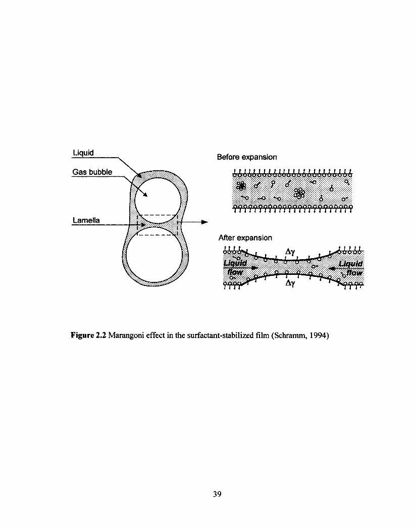
Liquid Before expansion
4sMAY4.4:44:44.:444.44444:4:4
After expansion
Figure 2.2 Marangoni effect in the surfactant-stabilized film (Schramm, 1994)
39
Liquid
Gas bubble
Lame a
Before expansion
m * f r fs&~ 4 " •S> w> N> *QP 6 c*
ja£U3Yt««W2«xi£U2!£LQCfcQiCLDlX2£LQS[Xltt y y y y v y v v v y i y y y y y y y y y y y y y
After expansion
iife UWHt
H i ' ? I J \ftow
Liquid
Figure 2.2 Marangoni effect in the surfactant-stabilized film (Schramm, 1994)
39

2.2 Buckingham Pi-theorem
The Buckingham Pi-theorem established by Buckingham in 1914 has been well-
recognized as a fundamental theorem in dimensional analysis (Buckingham, 1914). It
involves establishment of a mathematical procedure to obtain a series of dimensionless
parameters from a certain number of physical variables describing a physical system or
phenomenon of interest. With the assumption of having all the ratios of the physical
variables constant, the physical phenomenon can be described as:
AQ/, Q2, • • •, Qn) = 0 (2.5)
where Q is the physical variable(s). The dimensionless parameter (1l) is defined as:
II nl val n2a2
— vn nan
v (2.6)
where al, a2, a„ are the exponents of each physical variable that must satisfy the
principle of dimensional homogeneity. As a result, the physical system is alternatively
expressed as a function of the dimensionless parameters as shown in the following
expression:
F(11, n2,..., fl ) = 0 (2.7)
The value of i must be determined since it represents the total number of dimensional
parameters that can be constructed from the original physical variables (Q1, Q2, • • •, Qn).
All the physical variables that are significant and influential to a specific system must
also be identified. The following are calculation steps to define each dimensionless
parameter:
(i) Breakdown the unit of all physical variables into fundamental units (e.g.,
mass, length, time, and temperature). The unit of each physical variable in
40
2.2 Buckingham Pi-theorem
The Buckingham Pi-theorem established by Buckingham in 1914 has been well-
recognized as a fundamental theorem in dimensional analysis (Buckingham, 1914). It
involves establishment of a mathematical procedure to obtain a series of dimensionless
parameters from a certain number of physical variables describing a physical system or
phenomenon of interest. With the assumption of having all the ratios of the physical
variables constant, the physical phenomenon can be described as:
AQi,Q2,...,Qn) = 0 (2.5)
where Q is the physical variable(s). The dimensionless parameter (IT) is defined as:
n = Q?Qp...QZ" (2.6)
where a/, 02, ..., a„ are the exponents of each physical variable that must satisfy the
principle of dimensional homogeneity. As a result, the physical system is alternatively
expressed as a function of the dimensionless parameters as shown in the following
expression:
F(n,,n2,...,110 = 0 (2.7)
The value of / must be determined since it represents the total number of dimensional
parameters that can be constructed from the original physical variables (Qi, Q2, ..., Qn).
All the physical variables that are significant and influential to a specific system must
also be identified. The following are calculation steps to define each dimensionless
parameter:
(i) Breakdown the unit of all physical variables into fundamental units (e.g.,
mass, length, time, and temperature). The unit of each physical variable in
40

Equation (2.6) could be either fundamental or derived (e.g., pascal, watt, cP,
etc.).
(ii) Determine the number of dimensional parameters (i) by
i = n k (2.8)
where n is the number of physical variables and k is the total number of
fundamental units needed to express the system.
(iii) Select k (out of n) physical variables (Qi, Q2,..., Qk) arbitrarily that have the
fundamental units as the basis for III, I12,...,
(iv) Incorporate one of the remaining physical variables (Qic+1, 0+2,- • •, Qn),
which mainly have derived units, into a set of k physical variables as
mentioned in Step (iii). This additional physical variable is defined as Si, S2,
S,. Then, the general form can be represented by:
[nii = [010..-QPsil [ll 2 = [Q1a2 Q: 2 S 2
• • • [nil= [Q,-Q2'...Qk'SrI
(2.9)
(v) Replace the unit of Q's and S by the fundamental units.
(vi) Find the values of all the exponents a, b, . . k for each dimensionless
parameter, which must eliminate all the fundamental units.
2.3 Literature review on the correlation of the pneumatic foam height
2.3.1 Application of Buckingham Pi-theorem
Several foaming semi-empirical equations have been extensively developed for
slag foaming systems using the Buckingham Pi-theorem. Ito and Fruehan (1989a and
41
Equation (2.6) could be either fundamental or derived (e.g., pascal, watt, cP,
etc.).
(ii) Determine the number of dimensional parameters (/') by
i = n-k (2.8)
where n is the number of physical variables and k is the total number of
fundamental units needed to express the system.
(iii) Select k (out of n) physical variables (Qi, 02,..., Qk) arbitrarily that have the
fundamental units as the basis for II|, it2,..., rij.
(iv) Incorporate one of the remaining physical variables (Qk+i, Qk+2Q»),
which mainly have derived units, into a set of k physical variables as
mentioned in Step (iii). This additional physical variable is defined as Si, S2,
Si. Then, the general form can be represented by:
[n,]=
[nj= jape? -a'-Sj] (2.9)
[n,]=[er &'...&*•s,]
(v) Replace the unit of Q's and S by the fundamental units.
(vi) Find the values of all the exponents a, b,..., k for each dimensionless
parameter, which must eliminate all the fundamental units.
23 Literature review on the correlation of the pneumatic foam height
2.3.1 Application of Buckingham Pi-theorem
Several foaming semi-empirical equations have been extensively developed for
slag foaming systems using the Buckingham Pi-theorem. Ito and Fruehan (1989a and
41

1989b) were the first to propose an empirical equation to predict a foaminess coefficient
for the CaO-SiO2-FeO with FeO content of 10-60 wt% at 1250-1400°C.
E=570 /4 Y slag P slag
(2.10)
where E is the foaminess coefficient (s) defined by Bikerman (1938 and 1973), ,u slag is
the slag viscosity (Pas), Ps/ag is the slag density (kg/m3), and ',wag is the slag surface
tension (N/m). From the equation, it was obvious that E was a strong function of
viscosity, which played a role in foam stability through deceleration of liquid drainage
from lamella in the foam, and E was inversely proportional to the square root of both
surface tension and density. This equation was expected to predict the slag foam
occurring in iron and steelmaking processes including oxygen steelmaking, electric
furnace steelmaking, and bath smelting. In 1991, Jiang and Fruehan extended Ito and
Fruehan's work to cover a lower range of FeO content of about 5 wt% at a higher
temperature of 1500°C, and they used more reliable methods to predict physical
properties (Jiang and Fruehan, 1991). They proposed an improved empirical equation,
shown below, which yielded higher accuracy in predicting E for the CaO-SiO2-FeO
system:
E = 115 slag Y slag P slag
(2.11)
This equation was later applied to predict foaming occurring in industrial bath smelting
processes without the presence of coke.
Zhang and Fruehan (1995) were the first to incorporate bubble diameter into foam
height correlation to account for the fact that foam morphology, one of the most
important parameters in foam stability, can be varied from sphere foam formed by small
42
1989b) were the first to propose an empirical equation to predict a foaminess coefficient
for the CaO-SiCh-FeO with FeO content of 10-60 wt% at 1250-1400°C.
£ = 570 . ^'ag (2.10) \ /slag r slag
where Z is the foaminess coefficient (s) defined by Bikerman (1938 and 1973), jusiag is
the slag viscosity (Pas), psiag is the slag density (kg/m3), and ystag is the slag surface
tension (N/m). From the equation, it was obvious that Z was a strong function of
viscosity, which played a role in foam stability through deceleration of liquid drainage
from lamella in the foam, and Z was inversely proportional to the square root of both
surface tension and density. This equation was expected to predict the slag foam
occurring in iron and steelmaking processes including oxygen steelmaking, electric
furnace steelmaking, and bath smelting. In 1991, Jiang and Fruehan extended Ito and
Fruehan's work to cover a lower range of FeO content of about 5 wt% at a higher
temperature of 1500°C, and they used more reliable methods to predict physical
properties (Jiang and Fruehan, 1991). They proposed an improved empirical equation,
shown below, which yielded higher accuracy in predicting Z for the Ca0-Si02-Fe0
system:
£ = 115 (2.11) y Yslag P stag
This equation was later applied to predict foaming occurring in industrial bath smelting
processes without the presence of coke.
Zhang and Fruehan (1995) were the first to incorporate bubble diameter into foam
height correlation to account for the fact that foam morphology, one of the most
important parameters in foam stability, can be varied from sphere foam formed by small
42

spherical bubbles to polyhedral foam composed of relatively large polyhedral bubbles
(Bikerman, 1938 and 1973). The bubble size was not accounted for in previous studies
(Equations 2.10-2.11) due to the small variation in bubble diameter of the foams
observed in their studies. Zhang and Fruehan developed the following correlation using
the bubble diameter as one of the independent parameters besides the physical properties
for a CaO-SiO2-FeO-A120 3 system with FeO content of 5-15 wt% at 1500°C:
.2 4" slag
E= 115 v 02 nsla g slag—
d av" e
(2.12)
where dare is the average bubble diameter (m). The model showed that E strongly
depended on viscosity; was inversely proportional to density and bubble diameter with
powers of -1.0 and -0.9, respectively; and was a weak function of surface tension. In
2000, Jung and Fruehan verified the above correlation (Equation (2.12)) by using it to
calculate E of the slag foaming for a CaO-SiO2-FeO-MgO system with a higher FeO
content of 10-32 wt% at 1400-1550°C. Although the predicted E was somewhat lower
than the experimental E due to the error from the prediction of liquid viscosity, this
correlation was still considered to adequately predict the foaming that occurred in this
particular system (Jung and Fruehan, 2000).
By performing dimensional analysis on their experimental results (Ghag et al.,
1998a), Ghag and his team recommended three different correlations for predicting E (s)
for an aqueous solution of glycerol containing a surfactant, sodium dodecylbenzene
sulphonate (SDBS), at 20°C (Ghag et al., 1998b):
A71.32E = 2.02 x10⁶ /4/ 2.32 3.64 (2.13)
43
spherical bubbles to polyhedral foam composed of relatively large polyhedral bubbles
(Bikerman, 1938 and 1973). The bubble size was not accounted for in previous studies
(Equations 2.10-2.11) due to the small variation in bubble diameter of the foams
observed in their studies. Zhang and Fruehan developed the following correlation using
the bubble diameter as one of the independent parameters besides the physical properties
for a Ca0-SiC>2-Fe0-Al203 system with FeO content of 5-15 wt% at 1500°C:
(2-12) / stag r slag ave
where dme is the average bubble diameter (m). The model showed that X strongly
depended on viscosity; was inversely proportional to density and bubble diameter with
powers of -1.0 and -0.9, respectively; and was a weak function of surface tension. In
2000, Jung and Fruehan verified the above correlation (Equation (2.12)) by using it to
calculate X of the slag foaming for a Ca0-Si02-Fe0-Mg0 system with a higher FeO
content of 10-32 wt% at 1400-1550°C. Although the predicted X was somewhat lower
than the experimental X due to the error from the prediction of liquid viscosity, this
correlation was still considered to adequately predict the foaming that occurred in this
particular system (Jung and Fruehan, 2000).
By performing dimensional analysis on their experimental results (Ghag et al.,
1998a), Ghag and his team recommended three different correlations for predicting X (s)
for an aqueous solution of glycerol containing a surfactant, sodium dodecylbenzene
sulphonate (SDBS), at 20°C (Ghag et al., 1998b):
X = 2.02 x10V; ( Ayi 32 ^ , „ \ 2.32 >3.64 (PLS) d ,
(2.13)
43

E°89 E=5.43x10⁵PL (pLes9d278
E=1.00x10⁶ pi ( Eeff 3 (pLg)d
(2.14)
(2.15)
where d is the bubble diameter (mm), PL is liquid viscosity (Pa's), PL is liquid density
(kg/m3), Ay is the surface tension depression equal to the difference between surface
tension of aqueous solution of glycerol with and without the SDBS (mN/m), EM is the
Marangoni dilational modulus (mN/m), which is the maximum surface elasticity of the
surface film, and Eeff is the effective elasticity (mN/m), which represents the true surface
elasticity. They suggested that E would depend on the surface tension depression in
Equation (2.13), the Marangoni dilational modulus in Equation (2.14), and the effective
elasticity in Equation (2.15) rather than the equilibrium surface tension, as previously
considered by Ito and Fruehan (1989b), Jiang and Fruehan (1991), and Zhang and
Fruehan (1995), since these properties better reflected the effect of viscoelastic forces on
foam stablity, which was induced by a variation in surface tension of the solution due to
the addition of surfactant. From the above correlations, they concluded that bubble size
had the greatest impact on the foam height, and Equation (2.15) best fitted with the
experimental data since a use of effective elasticity could naturalistically estimate the
degree of stability affected by the dynamic adsorption of surfactant. In 1998, Ghag et al.
(1998c) employed the experimental E of the slag foaming in the CaO-SiO2-FeO system
from Zhang and Fruehan (1995) to test the application of Equation (2.15) for a wider
range of physical properties and industrial practices. The results showed that the
predicted values did not show good agreement with the experimental data (Ghag et al.,
44
S = 5.43xl0Vi /
(2.14) (j>LgyMd 1.89 *2.78
V
(2.15)
where d is the bubble diameter (mm), /4 is liquid viscosity (Pa s), pi is liquid density
(kg/m3), Ay is the surface tension depression equal to the difference between surface
tension of aqueous solution of glycerol with and without the SDBS (mN/m), EM is the
Marangoni dilational modulus (mN/m), which is the maximum surface elasticity of the
surface film, and Eeff is the effective elasticity (mN/m), which represents the true surface
elasticity. They suggested that X would depend on the surface tension depression in
Equation (2.13), the Marangoni dilational modulus in Equation (2.14), and the effective
elasticity in Equation (2.15) rather than the equilibrium surface tension, as previously
considered by Ito and Fruehan (1989b), Jiang and Fruehan (1991), and Zhang and
Fruehan (1995), since these properties better reflected the effect of viscoelastic forces on
foam stablity, which was induced by a variation in surface tension of the solution due to
the addition of surfactant. From the above correlations, they concluded that bubble size
had the greatest impact on the foam height, and Equation (2.15) best fitted with the
experimental data since a use of effective elasticity could naturalistically estimate the
degree of stability affected by the dynamic adsorption of surfactant. In 1998, Ghag et al.
(1998c) employed the experimental Z of the slag foaming in the CaO-SiCVFeO system
from Zhang and Fruehan (1995) to test the application of Equation (2.15) for a wider
range of physical properties and industrial practices. The results showed that the
predicted values did not show good agreement with the experimental data (Ghag et al.,
44

1998c). In addition, it was difficult to measure these substituted physical properties by
simple techniques in order to use or validate their correlations.
Unlike the previous works, which applied dimensional analysis with an
application of the Buckingham-Pi theorem to a set of significant physical properties upon
which E depended, Pilon and his colleagues performed the analysis using the governing
equation of the foam layer proposed by Bhakta and Ruckenstein (1997) and presented the
following semi-empirical equation to predict the pneumatic steady-state foam height (H,
mm) under isothermal conditions (Pilon et al., 2001):
Ca(-1= Kr Rer
r L Fr ) (2.16)
where Re is the Reynolds number defined as PAO - Gm Kik, Fr is the Froude number
defined as (G — Gm )2/gr, Ca is the capillary number defined as it/JO - 6„, )1y, G is the
superficial gas velocity (mm/s), Gm is the minimum superficial gas velocity for the onset
of foaming (mm/s), r is the average bubble radius in the foam (mm), and K and N are the
adjustable parameters for a power-law relationship between two dimensionless groups
(i.e., lii = Ca(H/r) and U2 = Re/Fr), which in this case were 2905 and -1.80, respectively.
Consequently, the final correlation was written as:
H 2905 r 2r 6 0( [,UL (G -61'1
(Pa)(2.17)
This correlation was validated by foaming data available in the literature for a
high viscosity system with different types of dispersing gases (i.e., argon, air, N2, helium
and hydrogen) and diffusers (i.e., single and multiple orifice and Pyrex disk). It was
proven to be applicable to various systems with a broad range of physical properties (46
45
1998c). In addition, it was difficult to measure these substituted physical properties by
simple techniques in order to use or validate their correlations.
Unlike the previous works, which applied dimensional analysis with an
application of the Buckingham-Pi theorem to a set of significant physical properties upon
which X depended, Pilon and his colleagues performed the analysis using the governing
equation of the foam layer proposed by Bhakta and Ruckenstein (1997) and presented the
following semi-empirical equation to predict the pneumatic steady-state foam height (H,
mm) under isothermal conditions (Pilon et al., 2001):
where Re is the Reynolds number defined as pi{ G - Gm )r/jUL, Fr is the Froude number
defined as (G - Gm )2/gr, Ca is the capillary number defined as ML(G - Gm )!y, G is the
superficial gas velocity (mm/s), Gm is the minimum superficial gas velocity for the onset
of foaming (mm/s), r is the average bubble radius in the foam (mm), and K and N are the
adjustable parameters for a power-law relationship between two dimensionless groups
(i.e., Ill = Ca(H/r) and rh = Re/Fr), which in this case were 2905 and -1.80, respectively.
Consequently, the final correlation was written as:
This correlation was validated by foaming data available in the literature for a
high viscosity system with different types of dispersing gases (i.e., argon, air, N2, helium
and hydrogen) and diffusers (i.e., single and multiple orifice and Pyrex disk). It was
proven to be applicable to various systems with a broad range of physical properties (46
(2.16)
V /
(2.17)
45

< < 12100 mPas, 69.5 < y< 478 mN/m and 1200 < pc, < 3000 kg/m3), average bubble
size (0.7 < r < 20 mm), and superficial gas velocity (0 < G < 40 mm/s) within ±35%
error. The results of the sensitivity analysis on the average bubble radius, which was the
most influential parameter in predicting foam height according to Equation (2.17),
indicated that the predicted foam height could vary significantly within ±10% deviation
of the average bubble radius. As a result, it was suggested that bubble size distribution
replace the average bubble radius in future correlations. In addition, they recommended a
further investigation of the effect of initial liquid height through the minimum superficial
gas velocity since they observed a very large deviation between the predicted and
experimental values, particularly when small foam heights were measured at G
approaching Gm (Pilon et al., 2001). Note that Lotun and Pilon found that the use of the
Buckingham-Pi theorem with independent variables influencing the steady-state foam
height of the slag foam could lead to the same dimensionless numbers as those found by
non-dimensionalizing the governing equation (Equation (2.16)) (Lotun and Pilon, 2005).
2.3.2 Other approaches
Bikerman introduced the first foaming correlation for aqueous systems as
expressed below. The correlation predicts the foam height for aqueous solutions of n-
butyl alcohol dispersed by air (Bikerman, 1938 and 1973).
v HA H
G G G (2.18)
where v is the average steady foam volume (m3), H is pneumatic steady-state foam height
(m), G is the gas flow rate (m3/s), A is the cross-sectional area of the test cell (m2), and
46
< JUL< 12100 mPas, 69.5 < y< 478 mN/m and 1200 < pi< 3000 kg/m3), average bubble
size (0.7 < r < 20 mm), and superficial gas velocity (0 < G <40 mm/s) within ±35%
error. The results of the sensitivity analysis on the average bubble radius, which was the
most influential parameter in predicting foam height according to Equation (2.17),
indicated that the predicted foam height could vary significantly within ±10% deviation
of the average bubble radius. As a result, it was suggested that bubble size distribution
replace the average bubble radius in future correlations. In addition, they recommended a
further investigation of the effect of initial liquid height through the minimum superficial
gas velocity since they observed a very large deviation between the predicted and
experimental values, particularly when small foam heights were measured at G
approaching Gm (Pilon et al., 2001). Note that Lotun and Pilon found that the use of the
Buckingham-Pi theorem with independent variables influencing the steady-state foam
height of the slag foam could lead to the same dimensionless numbers as those found by
non-dimensionalizing the governing equation (Equation (2.16)) (Lotun and Pilon, 2005).
2.3.2 Other approaches
Bikerman introduced the first foaming correlation for aqueous systems as
expressed below. The correlation predicts the foam height for aqueous solutions of n-
butyl alcohol dispersed by air (Bikerman, 1938 and 1973).
(2., 8) G G G
where v is the average steady foam volume (m3), H is pneumatic steady-state foam height
(m), G is the gas flow rate (m3/s), A is the cross-sectional area of the test cell (m2), and
46
G is the superficial gas velocity (m/s). He found that E did not depend on gas flow rate,
experimental apparatus (dimension of test cell and size and porosity of diffusers),
incoming gas pressure, and solution volume when: 1) the solution volume was
sufficiently high to provide a certain depth to balance its rise due to gas bubbles and its
decrease due to the carryover of liquid into foam lamella and 2) the gas flow rate was in
the proper range, not so slow so as to cause little or no foam and not so fast so as to cause
any difficulties in obtaining readings either from rapid rupture or unstable position of the
upper foam boundary. He also claimed that E can be used as a physical property of the
solution with the unit of time indicating a residence time of gas traveling upward through
the foam or an average lifetime of foam before rupture. However, the application of
Equation (2.18) was limited within a certain range of the gas flow rate as mentioned
above. Therefore, the use of Equation (2.18) to explain foaming behaviour of the
solutions outside this particular range, especially at very low and high gas flow rates, is
questionable.
In recent years, more sophisticated foaming correlations have been developed, not
only to cover wider ranges of gas flow rates and physical properties of the liquid phase,
but also to account for the actual phenomenon of foam so that the prediction of the
steady-state foam height is more accurate and realistic. For example, Hrma considered
the facts that i) the foam height was determined by the bubbles at the top, which would
burst as soon as the liquid between the bubbles was drained out and the film thickness
reached the critical value and ii) the bubbles at the top of the foam layer must be ruptured
to balance new bubbles created by the incoming gas at the bottom of the layer so as to
maintain the steady-state condition of foam. As a result, he proposed the steady-state
47
G is the superficial gas velocity (m/s). He found that £ did not depend on gas flow rate,
experimental apparatus (dimension of test cell and size and porosity of diffusers),
incoming gas pressure, and solution volume when: 1) the solution volume was
sufficiently high to provide a certain depth to balance its rise due to gas bubbles and its
decrease due to the carryover of liquid into foam lamella and 2) the gas flow rate was in
the proper range, not so slow so as to cause little or no foam and not so fast so as to cause
any difficulties in obtaining readings either from rapid rupture or unstable position of the
upper foam boundary. He also claimed that X can be used as a physical property of the
solution with the unit of time indicating a residence time of gas traveling upward through
the foam or an average lifetime of foam before rupture. However, the application of
Equation (2.18) was limited within a certain range of the gas flow rate as mentioned
above. Therefore, the use of Equation (2.18) to explain foaming behaviour of the
solutions outside this particular range, especially at very low and high gas flow rates, is
questionable.
In recent years, more sophisticated foaming correlations have been developed, not
only to cover wider ranges of gas flow rates and physical properties of the liquid phase,
but also to account for the actual phenomenon of foam so that the prediction of the
steady-state foam height is more accurate and realistic. For example, Hrma considered
the facts that /) the foam height was determined by the bubbles at the top, which would
burst as soon as the liquid between the bubbles was drained out and the film thickness
reached the critical value and /'/') the bubbles at the top of the foam layer must be ruptured
to balance new bubbles created by the incoming gas at the bottom of the layer so as to
maintain the steady-state condition of foam. As a result, he proposed the steady-state
47

foaming correlation in 1990 to predict the foam height in terms of the bubble radius and
superficial gas velocity as shown below (Hrma, 1990):
-( 1 1
H = 2re.0" 1+ bhGm Gcr 1 (2.19) 1 1
6 Gcr
where ref is the effective average radius of bubble, bh is the constant, Gm is the threshold
gas flux or minimum superficial gas velocity required for the onset of foam, and 6, is
the critical superficial gas velocity at which the steady-state foam no longer exists. His
correlation presented the opportunity to eliminate the constraint of Equation (2.18) since
it can predict the foam height as the superficial velocity of the incoming gas ( 6 ) was
changed, i.e., (i) when G < 6„„ the foam was not formed in system, (ii) when G = 6„„
the foam height was equal to the diameter of the monolayer bubbles, (iii) when Gm < G
< 6„, the foam height was predicted by Equation (2.19), (iv) when G 6,, the foam
height was approaching infinity, which meant that the foam continuously increased
without a limit and consequently the steady-state condition could not be obtained. Even
though Hrma's correlation revealed more details of foaming behaviours, unclear
explanation of the constant bh together with the lack of the relationships to link the
physical properties of the solution into his correlation, led to a need for further
development.
Subsequently, Jeelani and his research team incorporated the effect of the binary
coalescence between gas bubbles into their foam height correlation to predict the foam
height of aqueous solutions of glycerine containing surfactants (Jeelani et al., 1990).
According to the material balance of liquid phase in the foam layer, liquid in the lamella
48
foaming correlation in 1990 to predict the foam height in terms of the bubble radius and
superficial gas velocity as shown below (Hrma, 1990):
H = 2rJ \ + b.
1 1 ^
1 1
G Gcr )
(2.19)
where reg is the effective average radius of bubble, bh is the constant, Gm is the threshold
gas flux or minimum superficial gas velocity required for the onset of foam, and Gcr is
the critical superficial gas velocity at which the steady-state foam no longer exists. His
correlation presented the opportunity to eliminate the constraint of Equation (2.18) since
it can predict the foam height as the superficial velocity of the incoming gas (G ) was
changed, i.e., (i) when G < Gm, the foam was not formed in system, (ii) when G = Gm,
the foam height was equal to the diameter of the monolayer bubbles, (iii) when Gm < G
< Gcr, the foam height was predicted by Equation (2.19), (iv) when G > Gcr, the foam
height was approaching infinity, which meant that the foam continuously increased
without a limit and consequently the steady-state condition could not be obtained. Even
though Hrma's correlation revealed more details of foaming behaviours, unclear
explanation of the constant bh together with the lack of the relationships to link the
physical properties of the solution into his correlation, led to a need for further
development.
Subsequently, Jeelani and his research team incorporated the effect of the binary
coalescence between gas bubbles into their foam height correlation to predict the foam
height of aqueous solutions of glycerine containing surfactants (Jeelani et al., 1990).
According to the material balance of liquid phase in the foam layer, liquid in the lamella
48
flowing back to the bulk solution (qd,,„„, m/s) was balanced by the liquid from the bulk
solution moving upward to the foam layer through the foam films (qupfibn, m/s) and the
Plateau borders (qup,pB, m/s) (Hartland and Barber, 1974). To avoid mathematical
complications, they divided the prediction into two cases. The first case was when qup,firm
was insignificant, which allowed qd w, to be equal to qup,pB, and the second case was
when qup,PB was insignificant, which allowed qdoi,„ to be equal to qupilan•
Case 1: qdown :4:- qup,pg since
K pc I 0 ) di.5
quizpg» qupium
2
H= eaveg„ 0.72s,u°L.75
K where p = '10.25 0.5 1 1 K2ci'"P O0.5 Wig) Y
65(5:reaverb„
Case 2: (Mown = qup, irm since qup,PB<< qupfilm
H = (6rb° +
cave (K fd,2.2560.25 (6Z" hod
ave
1 4.851.75e0•5r cr ave bo
where Kf = 0.138 s2 t425
gy .25 y
(2.20)
(2.21)
where H is pneumatic steady-state foam height (m); rbo and do are the binary coalescence
time (s) and the diameter of bubble entering the foam layer (m), respectively; G is the gas
flow rate per unit area (m3/m2-s); Kp and Kf are constants for Cases 1 and 2, respectively;
gar is the critical film thickness (m), which allows the coalescence to occur; say, is the
average gas fraction in the foam obtained by the y-ray attenuation technique; pc, is the
liquid viscosity (Pas); is the liquid density (kg/m3); y is the surface tension (N/m), and
s is the number of immobile surfaces, which number 2 for this system. By knowing a
change in the average bubble diameter along the foam height, the authors suggested that
49
flowing back to the bulk solution (qdown, m/s) was balanced by the liquid from the bulk
solution moving upward to the foam layer through the foam films (qupf,im, m/s) and the
Plateau borders (q^pB, m/s) (Hartland and Barber, 1974). To avoid mathematical
complications, they divided the prediction into two cases. The first case was when qup,jtim
was insignificant, which allowed qdown to be equal to qUP/>B, and the second case was
when qUPJPB was insignificant, which allowed qdown to be equal to qupjnm-
Case 1' qdown = quP,PB since qupjPB qupjiim
H =
Kpda
€ S K ave cr / G M.5
' f K2d2 ^ ^ 1
y6Scr£awTho j G05
^ o.i2sMr where Kp=- —
\PLS) y
Case 1". qdown = quP, iim since quP,PB qupjiin,
H = -c V ave /
+ -
r6
\ £<IV e
\~
Kfd™G0'25 ^ 0.8
. ^ 0.138^V125 where K , =
\0.25
(2.20)
(2.21)
where H is pneumatic steady-state foam height (m); Tb0 and d0 are the binary coalescence
time (s) and the diameter of bubble entering the foam layer (m), respectively; G is the gas
flow rate per unit area (m3/m2-s); Kp and K/ are constants for Cases 1 and 2, respectively;
Scr is the critical film thickness (m), which allows the coalescence to occur; w is the
average gas fraction in the foam obtained by the y-ray attenuation technique; fit is the
liquid viscosity (Pa s); pi is the liquid density (kg/m3); /is the surface tension (N/m), and
s is the number of immobile surfaces, which number 2 for this system. By knowing a
change in the average bubble diameter along the foam height, the authors suggested that
49

the steady-state foam height at a specified gas flow rate up to the critical value was a
function of gas flux, critical film thickness, binary coalescence time, bubble diameter and
liquid physical properties as expressed in Equations (2.20) — (2.21). The results clearly
showed that both equations could predict the experimental foam height reasonably well.
However, verifying the correlations was not possible since some experimental
parameters, such as the average gas-holdup fraction, could not be obtained from the
literature.
50
the steady-state foam height at a specified gas flow rate up to the critical value was a
function of gas flux, critical film thickness, binary coalescence time, bubble diameter and
liquid physical properties as expressed in Equations (2.20) - (2.21). The results clearly
showed that both equations could predict the experimental foam height reasonably well.
However, verifying the correlations was not possible since some experimental
parameters, such as the average gas-holdup fraction, could not be obtained from the
literature.
50

3. EXPERIMENTS
The foaming behaviours of the CO2-loaded aqueous solutions of alkanolamines
were investigated in both static and column foaming experiments, of which the details of
the experimental setups and procedures are given in Sections 3.1 and 3.2, respectively.
The key purpose of the former experiment was to carry out a parametric study to provide
the comprehensive information on the effects of process parameters on foaming
behaviours. The obtained experimental results were also used to develop the correlation
for prediction of pneumatic steady-state foam height (see details in Chapter 5). The latter
experiment was primarily aimed at generating experimental foam data used for foam
model verification (see details in Chapter 6).
3.1 Static foaming experiment
3.1.1 Experimental setup
The foaming experiments were carried out using the pneumatic method modified
from the standard ASTM D892 for foaming testing of lubricating oils (ASTM, 1999). As
shown in Figure 3.1, the setup was composed of a 1000 cm3 graduated cylinder cell, a
temperature bath with an immersion digital circulator with a stability of ±0.01°C in a
temperature ranging from 5°C above ambient temperature to 120°C, a metal diffuser
supplied from Petrolab Corp. (Latham, New York, U.S.), a polycarbonate drying column,
a flowmeter with an accuracy of ±2% full scale, and a gas mass flowmeter with an
accuracy ±1% full scale. The diffuser was made of sintered five micron porous stainless
steel with a maximum pore diameter not greater than 80 micron. Industrial grade N2
purchased from Praxair (Canada) was utilized as a dispersed gas to bubble the test
51
3. EXPERIMENTS
The foaming behaviours of the CC>2-loaded aqueous solutions of alkanolamines
were investigated in both static and column foaming experiments, of which the details of
the experimental setups and procedures are given in Sections 3.1 and 3.2, respectively.
The key purpose of the former experiment was to carry out a parametric study to provide
the comprehensive information on the effects of process parameters on foaming
behaviours. The obtained experimental results were also used to develop the correlation
for prediction of pneumatic steady-state foam height (see details in Chapter 5). The latter
experiment was primarily aimed at generating experimental foam data used for foam
model verification (see details in Chapter 6).
3.1 Static foaming experiment
3.1.1 Experimental setup
The foaming experiments were carried out using the pneumatic method modified
from the standard ASTM D892 for foaming testing of lubricating oils (ASTM, 1999). As
shown in Figure 3.1, the setup was composed of a 1000 cm3 graduated cylinder cell, a
temperature bath with an immersion digital circulator with a stability of ±0.01°C in a
temperature ranging from 5°C above ambient temperature to 120°C, a metal diffuser
supplied from Petrolab Corp. (Latham, New York, U.S.), a polycarbonate drying column,
a flowmeter with an accuracy of ±2% full scale, and a gas mass flowmeter with an
accuracy ±1% full scale. The diffuser was made of sintered five micron porous stainless
steel with a maximum pore diameter not greater than 80 micron. Industrial grade N2
purchased from Praxair (Canada) was utilized as a dispersed gas to bubble the test
51

solution instead of air. This was to prevent the degradation of alkanolamine that may
affect the foaming data obtained and also to maintain the CO2 loading of the test solution
during the experiments.
52
solution instead of air. This was to prevent the degradation of alkanolamine that may
affect the foaming data obtained and also to maintain the CO2 loading of the test solution
during the experiments.
52

Gas mass flowmeter
N2 cylinder
Emitted to atmosphere
Temperature bath
Figure 3.1 Schematic diagram of the static foaming experimental setup
Gas mass flowmeter Emitted to
atmosphere
Drying column
Test Cell
Immerse heater with thermometer
Flowmeter
Led
N2 cylinder Temperature bath
Figure 3.1 Schematic diagram of the static foaming experimental setup
53

3.1.2 Preparation of test solutions
Four single alkanolamines, MEA, DEA, MDEA, and AMP and three blended
alkanolamines, MEA+MDEA, DEA+MDEA, and MEA+AMP with mixing mole ratios
of 1:2, 1:1, and 2:1, respectively, were investigated in this study. These reagent-grade
alkanolamines were purchased from Sigma-Aldrich (Ontario, Canada). Their aqueous
solutions were prepared by diluting the reagent-grade alkanolamines to a desired
concentration using deionized water. The solution concentration was determined by
titration using a standard solution of 1 N hydrochloric acid (HCl) and methyl orange as
an indicator. The prepared solutions were loaded with CO2 by bubbling the industrial-
grade CO2 purchased from Praxair (Canada) through the fresh solutions of alkanolamines
for a certain period of time, depending on the desired CO2 loading in solution. The CO2
loading was determined using the standard method established by the Association of
Official Analytical Chemists (AOAC) (Horowitz, 1975). The details of chemicals and
gases used in this research are listed in Table 3.1.
54
3.1.2 Preparation of test solutions
Four single aikanolamines, ME A, DEA, MDEA, and AMP and three blended
aikanolamines, MEA+MDEA, DEA+MDEA, and MEA+AMP with mixing mole ratios
of 1:2, 1:1, and 2:1, respectively, were investigated in this study. These reagent-grade
aikanolamines were purchased from Sigma-Aldrich (Ontario, Canada). Their aqueous
solutions were prepared by diluting the reagent-grade aikanolamines to a desired
concentration using deionized water. The solution concentration was determined by
titration using a standard solution of 1 N hydrochloric acid (HC1) and methyl orange as
an indicator. The prepared solutions were loaded with CO2 by bubbling the industrial-
grade CO2 purchased from Praxair (Canada) through the fresh solutions of aikanolamines
for a certain period of time, depending on the desired CO2 loading in solution. The CO2
loading was determined using the standard method established by the Association of
Official Analytical Chemists (AOAC) (Horowitz, 1975). The details of chemicals and
gases used in this research are listed in Table 3.1.
54

Table 3.1 Source and purity of chemicals and gases
Chemical/gas Source Purity
MEA Sigma-Aldrich 99+%
DEA Sigma-Aldrich 99%
MDEA Sigma-Aldrich 99+%
AMP Sigma-Aldrich 95%
Acetic acid Sigma-Aldrich 99.7+%
Ammonium thiosulfate Sigma-Aldrich 99%
Bicine Sigma-Aldrich 99%
Copper (II) carbonate Sigma-Aldrich 98%
Formic acid Sigma-Aldrich 95 — 97%
Glycolic acid Sigma-Aldrich 99%
Hydrochloric acid EMD chemicals 36.5 — 38.0%
Malonic acid Sigma-Aldrich 99%
Oxalic acid Sigma-Aldrich 98%
Sodium chloride EMD chemicals 99%
Sodium metavanadate Sigma-Aldrich 90%
Sodium sulfite Fisher 99.3%
Sodium thiocyanate Sigma-Aldrich 98%
Sodium thiosulfate Sigma-Aldrich 99%
Sulfuric acid VWR 95 — 98%
Hydrochloric acid standard solution Fisher 1.000 mol/dm3
Methyl orange solution VWR 0.01%
CO2 Praxair 99.5%
N2 Praxair 99.995%
55
Table 3.1 Source and purity of chemicals and gases
Chemical/gas Source Purity
MEA Sigma-Aldrich 99+%
DEA Sigma-Aldrich 99%
MDEA Sigma-Aldrich 99+%
AMP Sigma-Aldrich 95%
Acetic acid Sigma-Aldrich 99.7+%
Ammonium thiosulfate Sigma-Aldrich 99%
Bicine Sigma-Aldrich 99%
Copper (II) carbonate Sigma-Aldrich 98%
Formic acid Sigma-Aldrich 95 - 97%
Glycolic acid Sigma-Aldrich 99%
Hydrochloric acid EMD chemicals 36.5 - 38.0%
Malonic acid Sigma-Aldrich 99%
Oxalic acid Sigma-Aldrich 98%
Sodium chloride EMD chemicals 99%
Sodium metavanadate Sigma-Aldrich 90%
Sodium sulfite Fisher 99.3%
Sodium thiocyanate Sigma-Aldrich 98%
Sodium thiosulfate Sigma-Aldrich 99%
Sulfuric acid VWR 95 - 98%
Hydrochloric acid standard solution Fisher 1.000 mol/dm"
Methyl orange solution VWR 0.01%
C02 Praxair 99.5%
n2 Praxair 99.995%
55

3.1.3 Experimental procedures
Prior to the experiments, the test solution was placed at a given volume (400 cm3
in most experimental runs) into the test cell without mechanical shaking or stirring, and
heated in a temperature bath to a set temperature for approximately 20 minutes. A metal
diffuser was inserted into the heated test cell and left for approximately 5 minutes to be
saturated with the test solution. N2 gas was then introduced to a polycarbonate drying
column to remove moisture before entering a flow meter for approximate measurement
and, subsequently, a mass flow meter for steady reading. The test solution was vigorously
bubbled by N2 gas through the gas diffuser with a blowing time of 25 min ± 5 seconds
(starting when the first N2 bubble rose from the gas diffuser). The N2 gas was eventually
released to the atmosphere from the outlet of the test cell. The concentration of
alkanolamine solution as well as its CO2 loading, conductivity, and pH were determined
before and after each experiment to ensure no changes occurred in the solution
constituents due to alkanolamine degradation products or variation in operating
conditions. During the blowing time, the foam volume above the gas dispersion layer (see
Figure 2.1, page 33) was recorded every minute. Such foam volume was in some cases
difficult to measure due to the unclear interface between the gas dispersion and the
Kugelschaum, the uneven Polyederfoam surface, and unpredictable foam rupture. As
such, average foam volumes at the 25th minute were then used (as shown in Figure 3.2)
instead of the actual foam volume to reduce errors due to data readings. It was found that
the average foam volume, in most experiments, began to reach a steady state after 10
minutes of blowing time. This steady value was, therefore, used as the representative
foam volume for subsequent data analysis.
56
3.1.3 Experimental procedures
Prior to the experiments, the test solution was placed at a given volume (400 cm3
in most experimental runs) into the test cell without mechanical shaking or stirring, and
heated in a temperature bath to a set temperature for approximately 20 minutes. A metal
diffiiser was inserted into the heated test cell and left for approximately 5 minutes to be
saturated with the test solution. N2 gas was then introduced to a polycarbonate drying
column to remove moisture before entering a flow meter for approximate measurement
and, subsequently, a mass flow meter for steady reading. The test solution was vigorously
bubbled by N2 gas through the gas diffuser with a blowing time of 25 min ± 5 seconds
(starting when the first N2 bubble rose from the gas diffiiser). The N2 gas was eventually
released to the atmosphere from the outlet of the test cell. The concentration of
alkanolamine solution as well as its CO2 loading, conductivity, and pH were determined
before and after each experiment to ensure no changes occurred in the solution
constituents due to alkanolamine degradation products or variation in operating
conditions. During the blowing time, the foam volume above the gas dispersion layer (see
Figure 2.1, page 33) was recorded every minute. Such foam volume was in some cases
difficult to measure due to the unclear interface between the gas dispersion and the
Kugelschaum, the uneven Polyederfoam surface, and unpredictable foam rupture. As
such, average foam volumes at the 25th minute were then used (as shown in Figure 3.2)
instead of the actual foam volume to reduce errors due to data readings. It was found that
the average foam volume, in most experiments, began to reach a steady state after 10
minutes of blowing time. This steady value was, therefore, used as the representative
foam volume for subsequent data analysis.
56

2.0
• 1.8
2 1.6 0
E • 1
'4
ea O E
1.2
te 11"f 1.0 co
0.8
& 0.6
• 0.4
0.2
0.0
• -I - • -*.-x- • *• • -* -x- • *• --x- •Yi- • -IX - X-- • -It- -x
5 10 15 20 25 Time (min)
Figure 3.2 Average foam volume profile during blowing time (MEA solution volume =
400 cm3, CO2 loading = 0.40 mol/mol, N2 velocity = 2.06 m3/m2-hr, MEA
concentration = 5.0 kmol/m3 and solution temperature = 40°C)
57
E 3 O > E <0 ^ O n £ E
"Sfe (0 0) D) & tt I
2.0
1.8
1.6
1.4
1.2
1.0
0.8
0.6
0.4
0.2
0.0
•O—o—^—O— . . . A . . . . © . — < • - " * " ™ * — - © • — « - o — - 0 — H .
-X- -x-:
-i 1 1 i 1 1 1 r- 1 1 1 1- i i 1 i
10 15 Time (min)
20 25
Figure 3.2 Average foam volume profile during blowing time (MEA solution volume:
400 cm3, CO2 loading = 0.40 mol/mol, N2 velocity = 2.06 m3/m2-hr, MEA
concentration =5.0 kmol/m3 and solution temperature = 40°C)
57
3.1.4 Data analysis
A foaminess coefficient (E, min) was calculated using the following equation
(Bikerman, 1973). It is a ratio of foam volume and superficial gas velocity, representing a
residence time of gas traveling upward through the foam or an average lifetime of foam
before rupture.
E 60v
GA (3.1)
where 6 is gas (N2) flow rate per unit area or superficial gas velocity (m3/m2-hr).
According to Bikerman (1973), the foaminess coefficient does not depend on gas flow
rate, dimension of test cell, solution volume, and pore size of diffuser if the solution
volume is deep enough and the superficial gas velocity is in a proper range. In this
research, the ranges of solution volume and superficial gas velocity are from 400 to 700
cm3 and from 1.75 to 2.41 m3/m2-hr, respectively.
3.1.5 Tested parameters and experimental conditions
A parametric study was carried out under a wide spectrum of operating
conditions. The parameters of interest are superficial gas velocity, solution volume,
alkanolamine concentration, CO2 loading of solution, solution temperature, degradation
product of alkanolamine, corrosion inhibitor, and alkanolamine type. Note that pressure
of the system was not included in the test program here. This is because it was reported to
have an insignificant effect on foaming tendency (Harruff, 1998). A summary of
parameters and experimental conditions is given in Table 3.2.
58
3.1.4 Data analysis
A foaminess coefficient (I, min) was calculated using the following equation
(Bikerman, 1973). It is a ratio of foam volume and superficial gas velocity, representing a
residence time of gas traveling upward through the foam or an average lifetime of foam
before rupture.
where G is gas (N2) flow rate per unit area or superficial gas velocity (m3/m2-hr).
According to Bikerman (1973), the foaminess coefficient does not depend on gas flow
rate, dimension of test cell, solution volume, and pore size of diffuser if the solution
volume is deep enough and the superficial gas velocity is in a proper range. In this
research, the ranges of solution volume and superficial gas velocity are from 400 to 700
cm3 and from 1.75 to 2.41 m3/m2-hr, respectively.
3.1.5 Tested parameters and experimental conditions
A parametric study was carried out under a wide spectrum of operating
conditions. The parameters of interest are superficial gas velocity, solution volume,
alkanolamine concentration, CO2 loading of solution, solution temperature, degradation
product of alkanolamine, corrosion inhibitor, and alkanolamine type. Note that pressure
of the system was not included in the test program here. This is because it was reported to
have an insignificant effect on foaming tendency (Harruff, 1998). A summary of
parameters and experimental conditions is given in Table 3.2.
58

Solution volume and superficial gas velocity were chosen as test parameters to
identify ranges with a constant E. Such ranges were used in the foaming tests for this
CO2-aqueous alkanolamine system, enabling the generation of foam data that are not
dependent on pore size of gas disperser, and dimension of test cell and ensuring the
consistency of foam data if solution volume and gas flow rate are changed within these
particular ranges. Due to its popularity in gas treating services, MEA was used as a
representative solvent in all foaming tests. Its concentration and CO2 loading cover
operating ranges in gas treating plants (Kohl and Nielson, 1997). Note that although the
MEA concentration of 7.0 kmol/m3 is not commonly used due to severe corrosion of
process equipment and piping, it is worth testing it here because such high MEA
concentrations present an opportunity for improved efficiency of the process and are thus
expected to be employed together with a corrosion inhibitor in the near future.
Solution temperatures up to 90°C were tested to simulate the temperatures of
various process components, such as the absorber, lean/rich heat exchanger, and cooler.
With the features of the test cell, foaming tests at temperatures beyond 90°C are not
applicable, as the CO2 loading of solution cannot be maintained under atmospheric
pressure. Nevertheless, the obtained data are adequate to reveal the effect of temperature
on foam tendency.
Thirteen degradation products were selected from the products reported in
published literature, including both regenerable compounds (i.e. bicine) (Rooney and
Dupart, 2000) and non-regenerable ones (i.e., carboxylic acids, sulfite, sulfate,
thiosulfate, thiocyanate and chloride) (Liu et al., 1995; Craig Jr. and McLaughlin, 1996;
Litschewski, 1996; Rooney et al., 1997; Fan et al., 2000). Sodium metavanadate
represents a toxic heavy-metal corrosion inhibitor commonly used in gas treating
59
Solution volume and superficial gas velocity were chosen as test parameters to
identify ranges with a constant £. Such ranges were used in the foaming tests for this
C02-aqueous alkanolamine system, enabling the generation of foam data that are not
dependent on pore size of gas disperser, and dimension of test cell and ensuring the
consistency of foam data if solution volume and gas flow rate are changed within these
particular ranges. Due to its popularity in gas treating services, MEA was used as a
representative solvent in all foaming tests. Its concentration and CO2 loading cover
operating ranges in gas treating plants (Kohl and Nielson, 1997). Note that although the
MEA concentration of 7.0 kmol/m3 is not commonly used due to severe corrosion of
process equipment and piping, it is worth testing it here because such high MEA
concentrations present an opportunity for improved efficiency of the process and are thus
expected to be employed together with a corrosion inhibitor in the near future.
Solution temperatures up to 90°C were tested to simulate the temperatures of
various process components, such as the absorber, lean/rich heat exchanger, and cooler.
With the features of the test cell, foaming tests at temperatures beyond 90°C are not
applicable, as the CO2 loading of solution cannot be maintained under atmospheric
pressure. Nevertheless, the obtained data are adequate to reveal the effect of temperature
on foam tendency.
Thirteen degradation products were selected from the products reported in
published literature, including both regenerable compounds (i.e. bicine) (Rooney and
Dupart, 2000) and non-regenerable ones (i.e., carboxyiic acids, sulfite, sulfate,
thiosulfate, thiocyanate and chloride) (Liu et al., 1995; Craig Jr. and McLaughlin, 1996;
Litschewski, 1996; Rooney et al., 1997; Fan et al., 2000). Sodium metavanadate
represents a toxic heavy-metal corrosion inhibitor commonly used in gas treating
59

industry, while copper carbonate and sodium sulfite represent low toxic ones.
Alkanolamine types, both single and blended-types, were also included in the test
program. In addition to MEA representing primary alkanolamine, DEA, MDEA, and
AMP were selected to represent secondary, tertiary, and sterically hindered
alkanolamines, respectively. Blended MEA+MDEA, DEA+MDEA, and MEA+AMP
were chosen because they are gaining a great deal of attention for their energy saving
characteristics. They represent mixtures of primary-tertiary, secondary-tertiary, and
primary-sterically hindered alkanolamines.
60

Table 3.2 Summary of tested parameters and operating conditions
Parameter Operating condition
Superficial gas (N2) velocity: 0.44 - 3.40 m3/m2-hr
2.0 and 5.0 kmol/m3 MEA, 400 cm3 solution volume, 0.40 mol/mol CO2 loading, and 40°C
Solution volume: 200 - 700 cm3
2.0 kmol/m3 MEA, 2.06 m3/m2-hr N2 velocity, 0.40 mol/mol CO2 loading, and 40°C
Alkanolamine concentration: 2.0 - 7.0 kmol/m3
CO2 loading: 0.10 - 0.55 mol/mol
MEA, 2.06 m3/m2-hr N2 velocity, 400 cm3 solution volume, 0.20 and 0.40 mol/mol CO2 loading, and 40°C 5.0 kmol/m3 MEA, 2.06 m3/m2-hr N2 velocity, 400 cm3solution volume, and 40, 60 and 90°C
Solution temperature: 40 - 90°C
5.0 kmol/m3 MEA, 2.06 m3/m2-hr N2 velocity, 400 cm3solution volume, and 0.20 and 0.40 mol/mol CO2 loading
Degradation product of MEA: acetic acid ammonium thiosulfate bicine formic acid glycolic acid hydrochloric acid malonic acid oxalic acid sodium chloride sodium sulfite (additive) sodium thiocyanate sodium thiosulfate sulfuric acid
10000 ppm of degradation product, 5.0 kmol/m3 MEA, 2.06 mi/m2-hr N2 velocity, 400 cm3 solution volume, 0.40 mol/mol CO2 loading, and 60°C
Corrosion inhibitor: copper carbonate sodium metavanadate sodium sulfite
1000 ppm of corrosion inhibitor, 5.0 kmol/m3 MEA, 2.06 m /m2-hr N2 velocity, 400 cm3 solution volume, 0.40 mol/mol CO2 loading, and 60°C
Alkanolamine type: MEA DEA MDEA AMP MEA+MDEA DEA+MDEA MEA+AMP
4.0 kmol/m3 alkanolamine, 2.06 m3/m2-hr N2 velocity, 400 cm3 solution volume, 0.40 mol/mol CO2 loading, 60°C, and mixing mole ratio of blended solution = 1:2, 1:1 and 2:1
61
Table 3.2 Summary of tested parameters and operating conditions
Parameter Operating condition
Superficial gas (N2) velocity: 0.44 - 3.40 m3/m2-hr
2.0 and 5.0 kmol/m3 MEA, 400 cm3 solution volume, 0.40 mol/mol CO2 loading, and 40°C
Solution volume: 200-700 cm3
2.0 kmol/m3 MEA, 2.06 m3/m2-hr N2 velocity, 0.40 mol/mol CO2 loading, and 40°C
Alkanolamine concentration: 2.0 - 7.0 kmol/m3
MEA, 2.06 m3/m2-hr N2 velocity, 400 cm3 solution volume, 0.20 and 0.40 mol/mol CO2 loading, and 40°C
CO2 loading: 0.10-0.55 mol/mol
5.0 kmol/m3 MEA, 2.06 m3/m2-hr N2 velocity, 400 cm3
solution volume, and 40, 60 and 90°C
Solution temperature: 40 - 90°C
5.0 kmol/m3 MEA, 2.06 m3/m2-hr N2 velocity, 400 cm3
solution volume, and 0.20 and 0.40 mol/mol CO2 loading
Degradation product of MEA: 10000 ppm of degradation product, 5.0 kmol/m3 MEA, acetic acid 2.06 m /m2-hr N2 velocity, 400 cm3 solution volume, ammonium thiosulfate 0.40 mol/mol CO2 loading, and 60°C bicine formic acid glycolic acid hydrochloric acid malonic acid oxalic acid sodium chloride sodium sulfite (additive) sodium thiocyanate sodium thiosulfate sulfuric acid
Corrosion inhibitor: 1000 ppm of corrosion inhibitor, 5.0 kmol/m3 MEA, copper carbonate 2.06 m /m2-hr N2 velocity, 400 cm3 solution volume, sodium metavanadate 0.40 mol/mol CO2 loading, and 60°C sodium sulfite
Alkanolamine type: 4.0 kmol/m3 alkanolamine, 2.06 m3/m2-hr N2 velocity, MEA 400 cm3 solution volume, 0.40 mol/mol CO2 loading, DEA 60°C, and mixing mole ratio of blended solution = 1:2, MDEA 1:1 and 2:1 AMP MEA+MDEA DEA+MDEA MEA+AMP
61

3.2 Column foaming experiment
3.2.1 Experimental setup
A series of foaming experiments, shown in Figure 3.3a, was carried out in a gas
absorption system mainly consisting of an absorber fitted with Mellapak 500.Y structured
packing, a solution buffer tank, solution pump, and gas filter and regulator. The absorber
was 0.80 m high and 0.10 m in diameter and made of acrylic plastic so as to allow visual
observation of foam generated during the experiments as shown in Figure 3.3b. Two
elements of Mellapak 500.Y were packed and arranged with 90° rotation. Their
geometric characteristics are provided in Table 3.3. The solution buffer tank was 0.02 m3
in volume and made of high-density polyethylene. The stainless steel gear pump
controlled by a digital dispensing drive was used to circulate the absorption solution with
±0.3% accuracy in flow rate. The liquid flow rate was regulated by a calibrated liquid
flow meter with a high-resolution valve. Feed gas (air) was regulated by a pressure
regulator providing a flow capacity of 15.0 scfm at 620 kPa and filtered by a 5-p.m
sintered brass element. A direct reading variable-area gas flow meter with a maximum
capacity of 8.0 scfm was used to measure gas flow rate. The temperatures of gas and
solution were measured using a J-KEM Model 210 temperature controller and K-type
thermocouples with a maximum error of ±0.4% on readings above 0°C. The foam heights
were measured using a measuring tape starting from the liquid level accumulated in the
outlet tubing at the bottom of the absorber.
62
3.2 Column foaming experiment
3.2.1 Experimental setup
A series of foaming experiments, shown in Figure 3.3a, was carried out in a gas
absorption system mainly consisting of an absorber fitted with Mellapak 500. Y structured
packing, a solution buffer tank, solution pump, and gas filter and regulator. The absorber
was 0.80 m high and 0.10 m in diameter and made of acrylic plastic so as to allow visual
observation of foam generated during the experiments as shown in Figure 3.3b. Two
elements of Mellapak 500.Y were packed and arranged with 90° rotation. Their
geometric characteristics are provided in Table 3.3. The solution buffer tank was 0.02 m3
in volume and made of high-density polyethylene. The stainless steel gear pump
controlled by a digital dispensing drive was used to circulate the absorption solution with
±0.3% accuracy in flow rate. The liquid flow rate was regulated by a calibrated liquid
flow meter with a high-resolution valve. Feed gas (air) was regulated by a pressure
regulator providing a flow capacity of 15.0 scfm at 620 kPa and filtered by a 5-jam
sintered brass element. A direct reading variable-area gas flow meter with a maximum
capacity of 8.0 scfm was used to measure gas flow rate. The temperatures of gas and
solution were measured using a J-KEM Model 210 temperature controller and K-type
thermocouples with a maximum error of ±0.4% on readings above 0°C. The foam heights
were measured using a measuring tape starting from the liquid level accumulated in the
outlet tubing at the bottom of the absorber.
62

Gas outlet
_l........
Absorber packed with structured packing
Gas inlet 4
\.., ./ Measuring
tape
Solution buffer tank
(a)
Air
[ -----°w1"---Filter
(b)
Figure 3.3 (a) Schematic diagram of the column foaming experimental apparatus and (b)
photograph of the absorber fitted with two elements of Mellapak 500.Y
(original in color)
63
m Gas outlet
Absorber packed with structured packing
Gas inlet
Measuring tape
Air Solution buffer tank Filter
(a) (b)
Figure 33 (a) Schematic diagram of the column foaming experimental apparatus and (b)
photograph of the absorber fitted with two elements of Mellapak 500. Y
(original in color)
63

Table 3.3 Geometric characteristics of Mellapak 500.Y
Geometric characteristics
Element height (hp, m) 0.205
Specific area (ap, m2/m3) 500
Void fraction 0.91
Corrugation angle (a, °) 45
Crimp height (hcrimp, 6.53x 10⁻³
Corrugation base (2B, m) 9.60x 10⁻³
Table 3.3 Geometric characteristics of Mellapak 500. Y
Geometric characteristics
Element height (hp, m) 0.205
Specific area (ap, m2/m3) 500
Void fraction 0.91
Corrugation angle (a, °) 45
Crimp height (h crimP, m) 6.53x10"3
Corrugation base (25, m) 9.60x10'3
64

3.2.2 Experimental procedures
Prior to the experiment, the aqueous MEA solution was prepared by diluting the
reagent-grade MEA (Sigma-Aldrich, Ontario, Canada) with deionized water to a desired
concentration and purging the solution with an industrial-grade CO2 (Praxair, Canada) to
a desired CO2 loading. After regulated to a given flow rate, a stream of air was
introduced to the bottom of the absorber through a filter to remove solid particles from
the stream, through a gas flow meter to measure gas flow rate, and through a
thermocouple to measure the temperature of feed air. The air then travelled upward and
countercurrently with the aqueous MEA solution, which was pumped from the storage
tank through the liquid flow meter and the thermocouple to the top of the absorber. The
solution was collected at the bottom of the column and recirculated. The reading of the
foam height was taken at the thirtieth minute after initiation of the experiment. Then, the
air and liquid temperature were respectively measured.
At the bottom of the column, a certain amount of foam, together with the liquid
solution, was gathered at the liquid outlet tube. In order to measure foam height in the
tube, the level of the accumulated solution above the outlet tube was, necessarily, kept to
the minimum so that all the foam was pushed down the tube as illustrated in Figure 3.4a.
The total foam height was the sum of the measured foam height, using the measuring tape
as shown in Figure 3.4b, and the distance from the top of the liquid outlet tube inside the
column to the measuring tape outside the column. This total foam height was used to
calculate the foam volume by multiplying the cross-sectional area of the tube with an
inside diameter of 9.5 mm. The experiment required repetition if the foam in the tube
coalesced into an air gap. During the experiment, if the solution level above the liquid
65

outlet tube was noticeably changed, some adjustment to the height of the tube was
necessary.
66
outlet tube was noticeably changed, some adjustment to the height of the tube was
necessary.
66
(a) (b)
Figure 3.4 Example of (a) a solution level above the liquid outlet tube at the bottom of
the column and (b) a foam height measurement (liquid velocity = 4.6
m3/m2-hr, air velocity = 120 mm/s and elapse time at =15 minutes)
(original in color)
67
(a) (b)
Figure 3.4 Example of (a) a solution level above the liquid outlet tube at the bottom of
the column and (b) a foam height measurement (liquid velocity = 4.6
m3/m2-hr, air velocity = 120 mm/s and elapse time at = 15 minutes)
(original in color)
67

3.2.3 Experimental conditions
In the experiment, MEA was chosen as the absorption solvent due to its
popularity in the gas treating industry and its potential for post-combustion carbon
capture (Tzimas and Peteves, 2003; Metz et al., 2005). In addition, the aqueous MEA
solution with concentration and CO2 loading of 5.0 kmollm3 and 0.40 mol/mol,
respectively, was reported to induce higher foaming tendency than other alkanolamine
solutions (see Sections 4.3 and 4.4). To eliminate the effect of mass transfer on the
foaming results, air was used to disperse the preloaded aqueous MEA solution.
Experimental conditions are summarized in Table 3.4. Note that both tested gas and
liquid flow rates provide liquid-to-gas (LIG) ratios ranging from 0.6 to 18.9 (kg
solution/kg air), which cover the LIG ratio range used in the CO2 capture pilot plant at the
Esbjerg coal-fired power plant (Knudsen et al., 2009).
68
3.2.3 Experimental conditions
In the experiment, MEA was chosen as the absorption solvent due to its
popularity in the gas treating industry and its potential for post-combustion carbon
capture (Tzimas and Peteves, 2003; Metz et al., 2005). In addition, the aqueous MEA
solution with concentration and CO2 loading of 5.0 kmol/m3 and 0.40 mol/mol,
respectively, was reported to induce higher foaming tendency than other alkanolamine
solutions (see Sections 4.3 and 4.4). To eliminate the effect of mass transfer on the
foaming results, air was used to disperse the preloaded aqueous MEA solution.
Experimental conditions are summarized in Table 3.4. Note that both tested gas and
liquid flow rates provide liquid-to-gas (L/G) ratios ranging from 0.6 to 18.9 (kg
solution/kg air), which cover the L/G ratio range used in the CO2 capture pilot plant at the
Esbjerg coal-fired power plant (Knudsen et al., 2009).
68
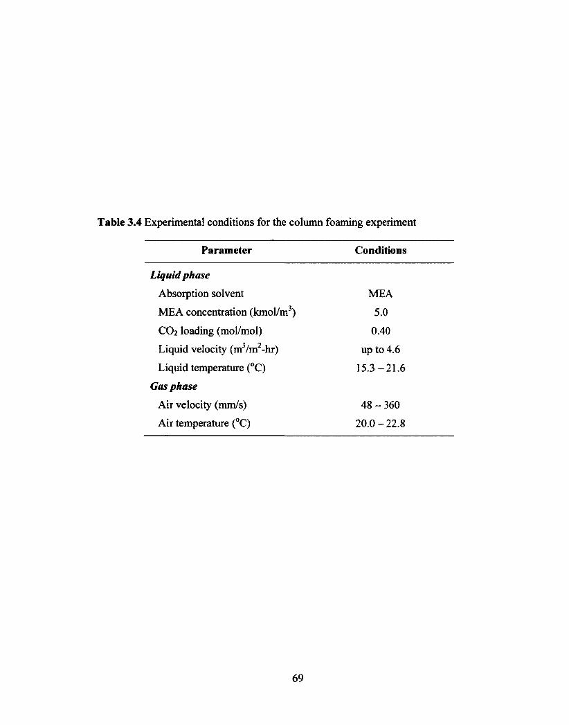
Table 3.4 Experimental conditions for the column foaming experiment
Parameter Conditions
Liquid phase
Absorption solvent MEA
MEA concentration (lunol/m3) 5.0
CO2 loading (mol/mol) 0.40
Liquid velocity (m3/m2-hr) up to 4.6
Liquid temperature (°C) 15.3 — 21.6
Gas phase
Air velocity (mm/s) 48 — 360
Air temperature (°C) 20.0 — 22.8
Table 3.4 Experimental conditions for the column foaming experiment
Parameter Conditions
Liquid phase
Absorption solvent MEA
MEA concentration (kmol/m3) 5.0
CO2 loading (mol/mol) 0.40
Liquid velocity (m3/m2-hr) up to 4.6
Liquid temperature (°C) 15.3-21.6
Gas phase
Air velocity (mm/s) 48 - 360
Air temperature (°C) 20.0 - 22.8
69

4. PARAMETRIC STUDY ON FOAMING BEHAVIOUR
The parametric study provides a comprehensive set of foaming data under a wide
spectrum of operating conditions in the CO2 absorption process using aqueous solutions
of alkanolamines. The obtained data were reproducible with a standard deviation of 0.15
minutes and were, thus, sufficiently reliable to be used for revealing the effects of process
parameters on E and providing a better understanding of foaming behaviour. The
complete experimental results were given in Appendix A. Such data were also used to
develop an empirical correlation for the purpose of foaming prediction (see details in
Chapter 5).
4.1 Superficial gas velocity
N2 velocity was varied from 0.44 to 3.40 m3/m2-hr in both 2.0 and 5.0 kmol/m3
MEA solutions under 0.40 mol/mol CO2 loading at 40°C to investigate the effect of
velocity on E. The results in Figure 4.1 show that an increase in N2 velocity nonlinearly
decreases E. This is because the increasing turbulence created by the increasing gas
velocity disrupts foam formation and reduces foam stability.
As the N2 velocity is further increased to 1.75 m3/m2-hr or greater, E reaches
stabilization. This suggests that the volume of foam proportionally increases with N2
flow rate. Such gas velocity with a constant E presents an opportunity for the elimination
of the gas velocity effect on E in any foaming experiments. In this work, we, therefore,
chose to use a N2 velocity of 2.06 m3/m2-hr in all experimental runs.
70
4. PARAMETRIC STUDY ON FOAMING BEHAVIOUR
The parametric study provides a comprehensive set of foaming data under a wide
spectrum of operating conditions in the CO2 absorption process using aqueous solutions
of alkanolamines. The obtained data were reproducible with a standard deviation of 0.15
minutes and were, thus, sufficiently reliable to be used for revealing the effects of process
parameters on E and providing a better understanding of foaming behaviour. The
complete experimental results were given in Appendix A. Such data were also used to
develop an empirical correlation for the purpose of foaming prediction (see details in
Chapter 5).
4.1 Superficial gas velocity
N2 velocity was varied from 0.44 to 3.40 m3/m2-hr in both 2.0 and 5.0 kmol/m3
MEA solutions under 0.40 mol/mol CO2 loading at 40°C to investigate the effect of
velocity on 2. The results in Figure 4.1 show that an increase in N2 velocity nonlinearly
decreases S. This is because the increasing turbulence created by the increasing gas
velocity disrupts foam formation and reduces foam stability.
As the N2 velocity is further increased to 1.75 m3/m2-hr or greater, E reaches
stabilization. This suggests that the volume of foam proportionally increases with N2
flow rate. Such gas velocity with a constant I presents an opportunity for the elimination
of the gas velocity effect on 2 in any foaming experiments. In this work, we, therefore,
chose to use a N2 velocity of 2.06 m3/m2-hr in all experimental runs.
70

6.00
S WEN
5.00 -.
20 4.00 -IE m 00 3.000 m a) c 2.00 - .E m o u. 1.00 -
0.00 0.00
--0-- 2.0 kmoUm3
—43-- 5.0 kmoUm3
'a -ia.
-EL_ 0 - 13 - - - - la- ____ „.......
11............... ......:: :
1.00 2.00 3.00
Superficial gas velocity (m3/m2-hr)
4.00
Figure 4.1 Effect of superficial gas velocity on foaminess coefficients (MEA
concentration = 2.0 and 5.0 kmol/m3, solution volume = 400 cm3, CO2
loading = 0.40 mol/mol and solution temperature = 40°C)
71
6.00
| 5.00
•g 4.00 E o> g 3.00 CO CO
c 2.00 E (0 £ 1.00
0.00
—•— 2.0 kmol/m3
• — \ \ \ \ \ s *
5.0 kmol/m3
\ *
s \
* "El V O ""13' EJ---.
C ""'"--a
0.00 -i 1 1 r i 1 i 1 i 1 i
1.00 2.00 3.00
Superficial gas velocity (m3/m2-hr) 4.00
Figure 4.1 Effect of superficial gas velocity on foaminess coefficients (MEA
concentration = 2.0 and 5.0 kmol/m3, solution volume = 400 cm3, CO2
loading = 0.40 mol/mol and solution temperature = 40°C)
71

4.2 Solution volume
The effect of solution volume on E was investigated by varying the solution volume
of a 2.0 kmol/m3 MEA solution containing 0.40 mol/mol CO2 loading from 200 to 700
cm3 at 40°C and 2.06 m3/m2-hr N2 velocity. The results shown in Figure 4.2 indicate that
foam formation does not occur when solution volume is 200 cm3. This is due to the
insufficient contact time for gas and liquid contact or due to an inadequate hydrostatic
force to resist the buoyancy force of a N2 bubble (Figure 4.3). As a result, the bubble
detaches from the diffuser and induces a turbulent flow among bubbles in the test cell.
The shearing force caused by this turbulence may destroy the foams. Once the solution
volume increases to more than 200 cm3, foams are produced and E increases with
solution volume. This is because the increase in solution volume leads to an increase in
hydrostatic force, which in turn reduces the turbulence caused by the bubble detachment
from the diffuser. As the solution volume is further increased from 400 to 700 cm3, E
becomes invariant. This is because the increasing hydrostatic force overcomes the
turbulence caused by the bubble detachment or makes such turbulence insignificant.
Gravity drainage is also retarded because an increase in solution volume increases the
thickness of the lamella. This eventually helps reduce foam collapse in the system. The
above findings suggest that solution volume should not be chosen arbitrarily for foaming
experiments since different values of foam volume and E can be obtained under identical
operating conditions. To eliminate such effects of solution volume, the solution volume
resulting in a steady E (i.e., > 400 cm3) should be used. In this work, we, therefore,
selected a solution volume of 400 cm3 for all experimental runs.
72
4.2 Solution volume
The effect of solution volume on 2 was investigated by varying the solution volume
of a 2.0 kmol/m3 MEA solution containing 0.40 mol/mol CO2 loading from 200 to 700
cm3 at 40°C and 2.06 m3/m2-hr N2 velocity. The results shown in Figure 4.2 indicate that
foam formation does not occur when solution volume is 200 cm3. This is due to the
insufficient contact time for gas and liquid contact or due to an inadequate hydrostatic
force to resist the buoyancy force of a N2 bubble (Figure 4.3). As a result, the bubble
detaches from the diffuser and induces a turbulent flow among bubbles in the test cell.
The shearing force caused by this turbulence may destroy the foams. Once the solution
•j volume increases to more than 200 cm , foams are produced and S increases with
solution volume. This is because the increase in solution volume leads to an increase in
hydrostatic force, which in turn reduces the turbulence caused by the bubble detachment
from the diffuser. As the solution volume is further increased from 400 to 700 cm3, Z
becomes invariant. This is because the increasing hydrostatic force overcomes the
turbulence caused by the bubble detachment or makes such turbulence insignificant.
Gravity drainage is also retarded because an increase in solution volume increases the
thickness of the lamella. This eventually helps reduce foam collapse in the system. The
above findings suggest that solution volume should not be chosen arbitrarily for foaming
experiments since different values of foam volume and X can be obtained under identical
operating conditions. To eliminate such effects of solution volume, the solution volume
resulting in a steady £ (i.e., > 400 cm3) should be used. In this work, we, therefore,
selected a solution volume of 400 cm3 for all experimental runs.
72

1.00
S •.... E 0.80
61a) .0— 0.60 m o m m 0.40 m c .E al 0.20 o u-
0.00 0 200 400
Solution volume (cm3)
600 800
Figure 4.2 Effect of solution volume on foaminess coefficients (MEA concentration =
2.0 kmol/m3, N2 velocity = 2.06 m3/m2-hr, CO2 loading = 0.40 mol/mol and
solution temperature = 40°C)
73
1.00
E 0.80
0.60
0.40
0.20 u.
0.00 0 200 400 600 800
Solution volume (cm3)
Figure 4.2 Effect of solution volume on foaminess coefficients (MEA concentration =
2.0 kmol/m3, N2 velocity = 2.06 m3/m2-hr, CO2 loading = 0.40 mol/mol and
solution temperature = 40°C)
73

Liquid
Hydrostatic force
l irBuoyancy Surface
force force
t
Gas
Solid
Figure 4.3 Three principal forces influencing bubble formation
74
Liquid
Hydrostatic force
\ Buoyancy Surface
force force
Solid
Figure 4.3 Three principal forces influencing bubble formation
74

4.3 Alkanolamine concentration
The concentration of aqueous MEA solution was varied from 2.0 to 7.0 kmol/m3
under two operating conditions of the absorber (i.e., 0.20 mol/mol CO2 loading and 40°C
representing the conditions of the absorber top and 0.40 mol/mol CO2 loading and 60°C
representing the conditions of the absorber bottom). The results in Figure 4.4 show that E
initially increases with MEA concentration and then declines after the MEA
concentration reaches 3.0 and 6.0 kmol/m3 in the cases of the absorber top and bottom,
respectively.
The increase in E with MEA concentration is due to a decrease in surface tension
of solution (Figure 4.5a). When the surface tension is decreased, the surface force is
lowered and overcome by the buoyancy force of the foam bubble. This then results in
greater foam volume and E. In addition to the surface tension, the density and viscosity of
MEA solution are also attributable to the increase in E. The higher concentration of MEA
solution increases the density and the bulk viscosity of the solution (Figures 4.5b-4.5c).
The increased solution density increases the buoyancy force of the foam bubble, while
the increased bulk viscosity retards the foam collapse caused by gravity drainage. Both
effects lead to a greater E.
As mentioned previously, E not only increases but also decreases with MEA
concentration when the MEA concentration is greater than 3.0 and 6.0 kmol/m3 under the
conditions of the absorber top and bottom, respectively. This is a result of the creaming
process (Walstra, 1989), wherein bulk viscosity plays a significant role on the rising
bubbles through the liquid phase to form a foam layer. According to the Stokes' equation,
75
4.3 Alkanolamine concentration
The concentration of aqueous MEA solution was varied from 2.0 to 7.0 kmol/m3
under two operating conditions of the absorber (i.e., 0.20 mol/mol CO2 loading and 40°C
representing the conditions of the absorber top and 0.40 mol/mol CO2 loading and 60°C
representing the conditions of the absorber bottom). The results in Figure 4.4 show that E
initially increases with MEA concentration and then declines after the MEA
concentration reaches 3.0 and 6.0 kmol/m3 in the cases of the absorber top and bottom,
respectively.
The increase in £ with MEA concentration is due to a decrease in surface tension
of solution (Figure 4.5a). When the surface tension is decreased, the surface force is
lowered and overcome by the buoyancy force of the foam bubble. This then results in
greater foam volume and E. In addition to the surface tension, the density and viscosity of
MEA solution are also attributable to the increase in E. The higher concentration of MEA
solution increases the density and the bulk viscosity of the solution (Figures 4.5b-4.5c).
The increased solution density increases the buoyancy force of the foam bubble, while
the increased bulk viscosity retards the foam collapse caused by gravity drainage. Both
effects lead to a greater X.
As mentioned previously, I not only increases but also decreases with MEA
concentration when the MEA concentration is greater than 3.0 and 6.0 kmol/m3 under the
conditions of the absorber top and bottom, respectively. This is a result of the creaming
process (Walstra, 1989), wherein bulk viscosity plays a significant role on the rising
bubbles through the liquid phase to form a foam layer. According to the Stokes' equation,
75

an increase in bulk viscosity leads to an increase in drag force, which can retard or even
stop the rising bubbles. This thereby decreases foam formation in the solution.
Such decrease in E is also caused by a reduction of foam stability due to an
increase in surface viscosity of the solution. The increased viscosity can make the foam
surface more immobile and weakens the surface elasticity. As a result, the foam surface
has less ability to resist foam thinning and collapse.
76
an increase in bulk viscosity leads to an increase in drag force, which can retard or even
stop the rising bubbles. This thereby decreases foam formation in the solution.
Such decrease in £ is also caused by a reduction of foam stability due to an
increase in surface viscosity of the solution. The increased viscosity can make the foam
surface more immobile and weakens the surface elasticity. As a result, the foam surface
has less ability to resist foam thinning and collapse.
76

C
j 0.80 -
m 0.60 -C
0
1.0 2.0 3.0 4.0 5.0 6.0 7.0 8.0 MEA concentration (kmoUm3)
Figure 4.4 Effect of alkanolamine concentration on foaminess coefficient (N2 velocity =
2.06 m3/m2-hr, solution volume = 400 cm3, absorber top condition: CO2
loading = 0.20 mol/mol and solution temperature = 40°C, absorber bottom
condition: CO2 loading = 0.40 mol/mol and solution temperature = 60°C)
77
1.00
-c I o 0.80 o £ a> o 0 0)
« 0.60 c 1 a o LL
0.40
0.0 1.0 2.0 3.0 4.0 5.0 6.0 7.0 8.0 MEA concentration (kmol/m3)
Figure 4.4 Effect of alkanolamine concentration on foaminess coefficient (N2 velocity =
2.06 m3/m2-hr, solution volume = 400 cm3, absorber top condition: CO2
loading = 0.20 mol/mol and solution temperature = 40°C, absorber bottom
condition: CO2 loading = 0.40 mol/mol and solution temperature = 60°C)
—•— Absorber top
—Q— Absorber bottom 1 1 1 1 1 » 1 1 i 1 1 1 1 1 1 1 1 1 1 1 1—1—n—»—1 1 1—1—1—r
77

80 . c • o TA 70 - . 5?. E 60 ' C, 't= 50 -w •
40 0.0 2.0 4.0 6.0 8.0
MEA concentration (kmol/m3)
1.12
• 1.10 c O ̂ 1.08 la n E d.21.06
4 a) ".5 1.04
a. 1.02
1.00
(a)
0.0 2.0 4.0 6.0 8.0 MEA concentration (kmol/m3)
(b) 4.0
P 3.0 - o c..) ..._O 0
> oi 2.0 --a a. I; E •
.-- • 1 0 - V
a. 0.0
0.0 2.0 4.0 6.0 8.0 MEA concentration (kmol/m3)
(c)
Figure 4.5 (a) Surface tension of the CO2-unloaded aqueous MEA solution replotted
from the experimental data (Vazquez et al., 1997), (b) predicted density of the
CO2-loaded MEA solution from correlation (Weiland et al., 1998) and (c)
predicted viscosity of the CO2-loaded aqueous MEA solutions from
correlation (Weiland et al., 1998)
78
2.0 4.0 6.0 8.0 MEA concentration (kmol/m3)
(a)
-B" Bottom
.0 2.0 4.0 6.0 8.0 MEA concentration (kmol/m3)
(b)
& I 3 o £ M > « 2. T3 a. 0 c 4-* c
1 1
e a.
0.
0
0
.0
.0
.0
— T o p --Q-- Bottom
//
O"
0.0 2.0 4.0 6.0 8.0 MEA concentration (kmol/m3)
(c)
Figure 4.5 (a) Surface tension of the CCVunloaded aqueous MEA solution replotted
from the experimental data (Vazquez et al., 1997), (b) predicted density of the
CC>2-loaded MEA solution from correlation (Weiland et al., 1998) and (c)
predicted viscosity of the CC^-loaded aqueous MEA solutions from
correlation (Weiland et al., 1998)
78

4.4 CO2 loading
The effect of CO2 loading of solution on E was studied using a 5.0 kmol/m3
aqueous MEA solutions under three different temperatures of 40, 60 and 90°C and CO2
loading ranging from 0.10 to 0.55 mol/mol. The results in Figure 4.6 show that an
increase in CO2 loading increases E for all temperatures. This can be explained by the
surface tension and density of the solution. As the CO2 loading increases, the surface
tension decreases (Figure 4.7a) and the solution density increases (Figure 4.7b). This
results in a reduced surface force and an increased buoyancy force, which, thus, promotes
foam formation and causes a greater E. Such increase in E is also due to an enhancement
of foam stability caused by an increase in bulk viscosity (Figure 4.7c) preventing the
thinning process and by an existence of a surface tension gradient promoting the
Marangoni effect. As CO2 loading increases, this surface tension gradient becomes
larger, which in turn enhances the Marangori effect. In addition to the above increasing
trend of E, the results in Figure 4.6 also show a decreasing trend of E after the CO2
loading is increased to a certain value. This is primarily due to the influence of solution
viscosity, which becomes more significant than those of surface tension and density. At a
higher CO2 loading, solution viscosity is increased (Figure 4.7c), thereby discouraging
foam formation. The higher solution viscosity also reflects a greater surface viscosity,
which in turn results in a reduction in foam stability.
79
4.4 CO2 loading
The effect of CO2 loading of solution on E was studied using a 5.0 kmol/m3
aqueous MEA solutions under three different temperatures of 40, 60 and 90°C and CO2
loading ranging from 0.10 to 0.55 mol/mol. The results in Figure 4.6 show that an
increase in CO2 loading increases 2 for all temperatures. This can be explained by the
surface tension and density of the solution. As the CO2 loading increases, the surface
tension decreases (Figure 4.7a) and the solution density increases (Figure 4.7b). This
results in a reduced surface force and an increased buoyancy force, which, thus, promotes
foam formation and causes a greater 2. Such increase in 2 is also due to an enhancement
of foam stability caused by an increase in bulk viscosity (Figure 4.7c) preventing the
thinning process and by an existence of a surface tension gradient promoting the
Marangoni effect. As CO2 loading increases, this surface tension gradient becomes
larger, which in turn enhances the Marangori effect. In addition to the above increasing
trend of I, the results in Figure 4.6 also show a decreasing trend of £ after the CO2
loading is increased to a certain value. This is primarily due to the influence of solution
viscosity, which becomes more significant than those of surface tension and density. At a
higher CO2 loading, solution viscosity is increased (Figure 4.7c), thereby discouraging
foam formation. The higher solution viscosity also reflects a greater surface viscosity,
which in turn results in a reduction in foam stability.
79

1.50
S •_ E
CI2 1.00 -
E o o o a 6 2 0.50 -
•Eas 0 LL
0.00 0.00 0.10 0.20 0.30 0.40 0.50 0.60
CO2loading in solution (mol CO2/mol MEA)
Figure 4.6 Effect of CO2 loading on foaminess coefficient (MEA concentration = 5.0
kmoi/m3, N2 velocity = 2.06 m3/m2-hr, solution volume = 400 cm3 and
solution temperature = 40, 60 and 90°C)
80
1.50
I
J 1.00 o
SE ® o 0 (0 (0 ® 0.50
1 •s o UL
0.00 0.00 0.10 0.20 0.30 0.40 0.50 0.60
C02 loading in solution (mol C02/mol MEA)
40°C •--- 60°C *— 90°C
-or a •
Figure 4.6 Effect of CO2 loading on foaminess coefficient (MEA concentration = 5.0
kmol/m3, N2 velocity = 2.06 m3/m2-hr, solution volume = 400 cm3 and
solution temperature = 40,60 and 90°C)
80

65 0 2 —.60 -
E
3 E 66 - ea
u) • 60
45 0.00 0.20 0.40 0.60
CO2 loading (mol CO2/mol MEA)
- 2 kmoUm3, 40°C 2 kmoUm3, 60°C
— •X• • - 3 kmoUm3, 40°C - -d 3kmoUm3, 60°C
(a) 1.16 .
1.12 my •o
11.08 2 -a, •-1.04 Iv 0. 1.00
0.96 • • • . 0.00 0.20 0.40 0.60 CO2 loading (mol CO2/mol MEA)
(b) 4.0
713 3.0 -
co > ca 1, E 0- 2.0 - a ••• „
a. x_ _ _ _x__ 31;_ • * E •
0.0 0.00 0.20 0.40 0.60 CO2 loading (mol CO2/mol MEA)
(c)
Figure 4.7 (a) Surface tension of the CO2-loaded aqueous MEA solution as a function of CO2 loading and solution temperature (measured by Spinning Drop Interfacial Tensiometer Model 510), (b) predicted density of 5.0 kmol/m3 MEA solution from correlation (Weiland et al., 1998), and (c) predicted viscosity of 5.0 kmol/m3 MEA solution from correlation (Weiland et al., 1998)
81
o » «! •I o E. •c 3 to
65
.60
55
50
45
—* ft— — —a
—•— 2 kmol/m3, 40°C —G— 2 kmol/m3, 60°C - * - 3 kmol/mJ, 40°C --A-- 3 kmol/m3, 60°C
0.00 0.20 0.40 0.60 C02 loading (mol CO^mol MEA)
(a)
-Q— 60°C
0.00 0.20 0.40 0.60 C02 loading (mol COj/mol MEA)
(b)
0.0
- 40°C —•&— 60°C - * - 90°C
„Q-0E0
0.00 0.20 0.40 0.60 C02 loading (mol COj/mol MEA)
(c)
Figure 4.7 (a) Surface tension of the C02-loaded aqueous MEA solution as a function of CO2 loading and solution temperature (measured by Spinning Drop Interfacial Tensiometer Model 510), (b) predicted density of 5.0 kmol/m3 MEA solution from correlation (Weiland et al., 1998), and (c) predicted viscosity of 5.0 kmol/m3 MEA solution from correlation (Weiland et al., 1998)
81

4.5 Solution temperature
Solution temperature was found to have a significant effect on E. As seen from
Figure 4.8, as the temperature of 5.0 kmol/m3 MEA solutions increased from 40 to 90°C,
E decreased considerably. This is true for both systems containing 0.20 and 0.40 mol/mol
CO2 loading. Such an effect is a result of poor foam stability, which is caused by reduced
bulk viscosity (Figure 4.9a) and a turbulence flow created by the vigorous movement of
molecules at an elevated temperature. Note that surface tension and density of the
solution play a minor role in such decreasing trends of E. As seen from Figures 4.9b-4.9c,
surface tension and density decrease with increasing temperature. This implies a lower
surface force (reflecting an enhancement of foam formation) and a lower buoyancy force
(reflecting a retardation of foam formation). The resulting force may be small or
insignificant compared to the influence of solution viscosity described above.
82
4.5 Solution temperature
Solution temperature was found to have a significant effect on E. As seen from
Figure 4.8, as the temperature of 5.0 kmol/m3 MEA solutions increased from 40 to 90°C,
2 decreased considerably. This is true for both systems containing 0.20 and 0.40 mol/mol
CO2 loading. Such an effect is a result of poor foam stability, which is caused by reduced
bulk viscosity (Figure 4.9a) and a turbulence flow created by the vigorous movement of
molecules at an elevated temperature. Note that surface tension and density of the
solution play a minor role in such decreasing trends of 2. As seen from Figures 4.9b-4.9c,
surface tension and density decrease with increasing temperature. This implies a lower
surface force (reflecting an enhancement of foam formation) and a lower buoyancy force
(reflecting a retardation of foam formation). The resulting force may be small or
insignificant compared to the influence of solution viscosity described above.
82

1.60
-a- 1.40 •E .--. 1.20 c .02 1.00 E 8 0.80 0 vi i 0.60 a) c 'E 0.40 Uo u 0.20
0.00 1 1 1
40.0
--•-- 0.20 mol CO2/mol MEA - - a - - 0.40 mol CO2/mol MEA
v ------____12
a 1 I 1 1 I 1 1 I I 1- 1 1 1 1 1 r t 1 1 -1-
50.0 60.0 70.0 80.0
Solution temperature (°C)
Figure 4.8 Effect of solution temperature on foaminess coefficient (MEA concentration
= 5.0 kmol/m3, N2 velocity = 2.06 m3/m2-hr, solution volume = 400 cm3 and
CO2 loading = 0.20 and 0.40 mol/mol)
90.0
83
1.60
<£ 1.40
~ 1.20
| 1.00 £ § 0.80 0 m 0.60 ® )
1 0.40 CO £ 0.20
0.00 40.0 50.0 60.0 70.0 80.0 90.0
Solution temperature (°C)
Figure 4.8 Effect of solution temperature on foaminess coefficient (MEA concentration
= 5.0 kmol/m3, N2 velocity = 2.06 m3/m2-hr, solution volume = 400 cm3 and
CO2 loading = 0.20 and 0.40 mol/mol)

2.5
2.0
-.4.4 1.5
3, lig 1.0
0.5 a.
0.0
70
0
a c
E 60 -
0 E CIS •••••••
50- a co
0.20 moUmol CO2 loading 0.40 moUmol CO2 loading
40.0 50.0 60.0 70.0 80.0 90.0
Solution temperature (°C)
40
20.0 30.0 40.0 50.0 60.0 Solution temperature (°C)
(a)
1.00
40.0 50.0 60.0 70.0 80.0 90.0 Solution temperature (°C)
(c)
Figure 4.9 (a) Predicted viscosity of 5.0 kmol/m3 MEA solution from correlation
(Weiland et al., 1998), (b) surface tension of 5.0 kmol/m3 unloaded-CO2
MEA solution replotted from experimental data (Vazquez et al., 1997), and
(c) predicted density of 5.0 kmol/m3 MEA solution from correlation (Weiland
et al., 1998)
(b)
0.20 moUmol CO2 loading -e--- 0.40 moUmol CO2 loading
5 ----- 19-- ---- -
84
"O £ Q.
0.5
0.0
-•— 0.20mol/moi CO2 loading -•B— Q.40 mol/mo< C02 loading
40.0 50.0 60.0 70.0 80.0 90.0 Solution temperature (°C)
(a)
20.0 30.0 40.0 50.0 60.0 Solution temperature (°C)
(b)
1.16 0.20 moi/mol CO2 loading
-B—- 0.40 moi/mol C02 loading
1.00 I I I
40.0 50.0 60.0 70.0 80.0 90.0 Solution temperature (°C)
(c)
Figure 4.9 (a) Predicted viscosity of 5.0 kmol/m3 MEA solution from correlation
(Weiland et al., 1998), (b) surface tension of 5.0 kmol/m3 unloaded-CCh
MEA solution replotted from experimental data (Vazquez et al., 1997), and
(c) predicted density of 5.0 kmol/m3 MEA solution from correlation (Weiland
et al., 1998)
84

4.6 Degradation products of MEA
The effect of thirteen degradation products on E was investigated by using a 5.0
kmol/m3 aqueous MEA solution containing 0.40 mol/mol CO2 loading at 60°C. The
results in Table 4.1 indicate that the solutions containing degradation products (except
sulfuric acid) provide a greater E than those without degradation products. Ammonium
thiosulfate induces the highest foam volume and E, followed by glycolic acid, sodium
sulfite, malonic acid, oxalic acid, sodium thiocyanate, sodium chloride, sodium
thiosulfate, bicine, hydrochloric acid, formic acid, acetic acid, and sulfuric acid.
The increase in E is due to formation of anionic surfactants in the presence of
sulfate (SO4- ), sulfonate ( SO;), and carboxylate (C00) functioning as a hydrophilic
group. These anionic surfactants reduce surface tension of the solution, thereby
encouraging foam formation. Such surfactants also enhance foam stability by improving
surface elasticity due to the Marangoni effect. The results also show that the presence of
chloride ions increases E. This is probably because the chloride ions reduce surface
tension by neutralizing the ionic products resulting from the reaction between CO2 and
MEA, which in turn enhances foam formation (Danckwerts and Tavares da Silva, 1967).
85
4.6 Degradation products of MEA
The effect of thirteen degradation products on E was investigated by using a 5.0
kmol/m3 aqueous MEA solution containing 0.40 mol/mol CO2 loading at 60°C. The
results in Table 4.1 indicate that the solutions containing degradation products (except
sulfuric acid) provide a greater I than those without degradation products. Ammonium
thiosulfate induces the highest foam volume and 2, followed by glycolic acid, sodium
sulfite, malonic acid, oxalic acid, sodium thiocyanate, sodium chloride, sodium
thiosulfate, bicine, hydrochloric acid, formic acid, acetic acid, and sulfuric acid.
The increase in 2 is due to formation of anionic surfactants in the presence of
sulfate (SO4"), sulfonate (SOj), and carboxylate (COO") functioning as a hydrophilic
group. These anionic surfactants reduce surface tension of the solution, thereby
encouraging foam formation. Such surfactants also enhance foam stability by improving
surface elasticity due to the Marangoni effect. The results also show that the presence of
chloride ions increases I. This is probably because the chloride ions reduce surface
tension by neutralizing the ionic products resulting from the reaction between CO2 and
MEA, which in turn enhances foam formation (Danckwerts and Tavares da Silva, 1967).
85

Table 4.1 Effect of degradation products on foaminess coefficient (degradation product
concentration = 10000 ppm, MEA concentration = 5.0 kmol/m3, N2 velocity =
2.06 m3/m2-hr, solution volume = 400 cm3, CO2 loading = 0.40 mol/mol and
solution temperature = 60°C)
Degradation product Average foaminess coefficient (min)1
None 0.79
Ammonium thiosulfate 0.97
Glycolic acid 0.94
Sodium sulfite 0.92
Malonic acid 0.92
Oxalic acid 0.90
Sodium thiocyanate 0.90
Sodium chloride 0.90
Sodium thiosulfate 0.85
Bicine 0.85
Hydrochloric acid 0.83
Formic acid 0.83
Acetic acid 0.82
Sulfuric acid 0.77 1 The maximum standard deviation of the foaminess coefficients is ±0.05 min.
86
Table 4.1 Effect of degradation products on foaminess coefficient (degradation product
concentration = 10000 ppm, MEA concentration = 5.0 kmol/m3, N2 velocity =
2.06 m3/m2-hr, solution volume = 400 cm3, C02 loading = 0.40 mol/mol and
solution temperature = 60°C)
Degradation product Average foaminess coefficient (min)1
None 0.79
Ammonium thiosulfate 0.97
Glycolic acid 0.94
Sodium sulfite 0.92
Malonic acid 0.92
Oxalic acid 0.90
Sodium thiocyanate 0.90
Sodium chloride 0.90
Sodium thiosulfate 0.85
Bicine 0.85
Hydrochloric acid 0.83
Formic acid 0.83
Acetic acid 0.82
Sulfuric acid 1 • ... -
0.77
86

4.7 Corrosion inhibitor
The effect of corrosion inhibitors on E was studied by adding three corrosion
inhibitors (i.e., sodium metavanadate, copper carbonate, and sodium sulfite) with a
concentration of 1000 ppm into a 5.0 kmol/m3 aqueous MEA solution containing 0.40
mol/mol CO2 loading. The results in Figure 4.10 clearly show that sodium metavanadate
and copper carbonate increase foam volume or E and sodium metavanadate induces a
greater effect, whereas sodium sulfite has no apparent effect. This can be explained by
considering the surface tension of aqueous MEA solutions. As shown in Table 4.2, the
surface tension values of aqueous MEA solutions are reduced when sodium
metavanadate and copper carbonate are added. However, a similar trend is not found for
sodium sulfite. For sodium sulfite, the surface tensions of the aqueous MEA solution with
and without the addition of sodium sulfite are not significantly different. This explains
why the foaming tendency of the aqueous MEA solution with sodium sulfite is somewhat
similar to that without sodium sulfite.
87
4.7 Corrosion inhibitor
The effect of corrosion inhibitors on I was studied by adding three corrosion
inhibitors (i.e., sodium metavanadate, copper carbonate, and sodium sulfite) with a
concentration of 1000 ppm into a 5.0 kmol/m3 aqueous MEA solution containing 0.40
mol/mol CO2 loading. The results in Figure 4.10 clearly show that sodium metavanadate
and copper carbonate increase foam volume or £ and sodium metavanadate induces a
greater effect, whereas sodium sulfite has no apparent effect. This can be explained by
considering the surface tension of aqueous MEA solutions. As shown in Table 4.2, the
surface tension values of aqueous MEA solutions are reduced when sodium
metavanadate and copper carbonate are added. However, a similar trend is not found for
sodium sulfite. For sodium sulfite, the surface tensions of the aqueous MEA solution with
and without the addition of sodium sulfite are not significantly different. This explains
why the foaming tendency of the aqueous MEA solution with sodium sulfite is somewhat
similar to that without sodium sulfite.
87

•
MEA
1.20 C' -1 1.00
I 0.80
0.60
0.40 0
0.20
0.00 MEA+NaVO3 MEA+CuCO3 MEA+Na2SO3
Corrosion inhibitor
Figure 4.10 Effect of corrosion inhibitors on foaminess coefficient (corrosion inhibitor =
NaVO3, CuCO3 and Na2SO3, corrosion inhibitor concentration = 1000 ppm,
MEA concentration = 5.0 kmol/m3, N2 velocity = 2.06 m3/m2-hr, solution
volume = 400 cm3, CO2 loading = 0.40 mol/mol and solution temperature =
60°C)
88
1.20
-§1.00 c © O 0.80 0 0 0) 0.60 <0
c 1 0.40
CO o u_
0.20
0.00 MEA MEA+NaV03 MEA+CuC03 MEA+Na2S03
Corrosion inhibitor
Figure 4.10 Effect of corrosion inhibitors on foaminess coefficient (corrosion inhibitor =
NaVC>3, C11CO3 and Na2SC>3, corrosion inhibitor concentration = 1000 ppm,
MEA concentration = 5.0 kmol/m3, N2 velocity = 2.06 m3/m2-hr, solution
volume = 400 cm3, CO2 loading = 0.40 mol/mol and solution temperature =
60°C)
88

Table 4.2 Surface tension of 5.0 kmol/m3 MEA solutions containing no CO2 loading at
25°C with/without 1000 ppm corrosion inhibitor (measured by KrOss
Tensiometer K100 using the Wilhelmy plate's principle)
System Surface tension (mN/m)
MEA without corrosion inhibitors 61.10 ± 0.02
MEA + sodium metavanadate 56.46 ± 0.03
57.67 ± 0.06
MEA + copper carbonate 58.63 ± 0.02
60.25 ± 0.01
MEA + sodium sulfite 62.51 ± 0.01
62.51 ± 0.01
89
Table 4.2 Surface tension of 5.0 kmol/m3 MEA solutions containing no CO2 loading at
25°C with/without 1000 ppm corrosion inhibitor (measured by KrOss
Tensiometer K100 using the Wilhelmy plate's principle)
System Surface tension (mN/m)
MEA without corrosion inhibitors 61.10 ±0.02
MEA + sodium metavanadate 56.46 ± 0.03
57.67 ± 0.06
MEA + copper carbonate 58.63 ± 0.02
60.25 ± 0.01
MEA + sodium sulfite 62.51 ±0.01
62.51 ±0.01
89
4.8 Alkanolamine type
Both single and blended alkanolamine solutions were tested for foaming tendency
using a 4.0 kmol/m3 total alkanolamine concentration containing 0.40 mol/mol CO2
loading at 60°C. The results for single alkanolamine solutions show that foam formation
occurs in MEA and MDEA but not in DEA and AMP solutions (Table 4.3). This implies
that surface force (represented by surface tension in Figure 4.11a) is overcome by
buoyancy force (represented by density in Figure 4.11b), and, consequently, bubbles can
be produced at the diffuser in the MEA and MDEA systems. E of MEA solution is
approximately 2.5 times that of MDEA solution since the rising bubbles in MEA solution
are easier to cream and form a layer of foam than those in MDEA solutions owing to the
lower solution viscosity of MEA solution than that of MDEA solution (Figure 4.11c).
From the observation, DEA and AMP solutions do not foam. It can be possibly explained
by a high bulk viscosity that could stop the bubbles from rising. Note that despite its high
viscosity, the MDEA solution may have foamed due to CO2 stripping as observed from
the decrease in CO2 loading of MDEA solution from 0.40 to 0.27 mol/mol during the
experiment.
For the blended alkanolamine solutions, only the MEA+AMP solution at a mixing
mole ratio of 2:1 has the potential to create foam, whereas MEA+MDEA and
DEA+MDEA solutions produce virtually no foam or only a trace amount at any mixing
ratio. This is because the surface tension of MEA+AMP is lower than that of
MEA+MDEA and DEA+MDEA at any mixing ratio (Figure 4.12a) and also because
MEA+AMP (Figure 4.12b) has the lowest bulk viscosity compared to the other blended
solutions. For the MEA+MDEA solutions, no foam is observed due to the high surface
tension (promoting less foam formation) and high bulk viscosity (hindering the creaming
90
4.8 Alkanolamine type
Both single and blended alkanolamine solutions were tested for foaming tendency
using a 4.0 kmol/m total alkanolamine concentration containing 0.40 mol/mol CO2
loading at 60°C. The results for single alkanolamine solutions show that foam formation
occurs in MEA and MDEA but not in DEA and AMP solutions (Table 4.3). This implies
that surface force (represented by surface tension in Figure 4.11a) is overcome by
buoyancy force (represented by density in Figure 4.1 lb), and, consequently, bubbles can
be produced at the diffuser in the MEA and MDEA systems. E of MEA solution is
approximately 2.5 times that of MDEA solution since the rising bubbles in MEA solution
are easier to cream and form a layer of foam than those in MDEA solutions owing to the
lower solution viscosity of MEA solution than that of MDEA solution (Figure 4.11c).
From the observation, DEA and AMP solutions do not foam. It can be possibly explained
by a high bulk viscosity that could stop the bubbles from rising. Note that despite its high
viscosity, the MDEA solution may have foamed due to CO2 stripping as observed from
the decrease in CO2 loading of MDEA solution from 0.40 to 0.27 mol/mol during the
experiment.
For the blended alkanolamine solutions, only the MEA+AMP solution at a mixing
mole ratio of 2:1 has the potential to create foam, whereas MEA+MDEA and
DEA+MDEA solutions produce virtually no foam or only a trace amount at any mixing
ratio. This is because the surface tension of MEA+AMP is lower than that of
MEA+MDEA and DEA+MDEA at any mixing ratio (Figure 4.12a) and also because
MEA+AMP (Figure 4.12b) has the lowest bulk viscosity compared to the other blended
solutions. For the MEA+MDEA solutions, no foam is observed due to the high surface
tension (promoting less foam formation) and high bulk viscosity (hindering the creaming
90

process of the bubbles). In addition, the unchanged in CO2 loading of these solutions
suggests that the effect of CO2 stripping plays no role in the foam formation as it does in
the MDEA solution.
91
process of the bubbles). In addition, the unchanged in CO2 loading of these solutions
suggests that the effect of CO2 stripping plays no role in the foam formation as it does in
the MDEA solution.
91

Table 4.3 Effect of alkanolamine type on foaminess coefficient (total alkanolamine
concentration = 4.0 kmol/m3, N2 velocity = 2.06 m3/m2-hr, solution volume =
400 cm3, CO2 loading = 0.40 mol/mol, solution temperature = 60°C and mixing
mole ratio of blended solution = 1:2, 1:1 and 2:1)
Type of alkanolamine Average foaminess coefficient (min)1
MEA 0.85
DEA No foam
MDEA2 0.32
AMP No foam
MEA + MDEA (1:2) No foam
MEA + MDEA (1:1) No foam
MEA + MDEA (2:1) No foam
DEA + MDEA (1:2) No foam
DEA + MDEA (1:1) No foam
DEA + MDEA (2:1) No foam
MEA + AMP (1:2) No foam
MEA + AMP (1:1) No foam
MEA + AMP (2:1) 0.13
I Maximum standard deviation of the foaminess coefficients is ±0.02 min. 2 Foam created by the MDEA solution could be a combined effect of CO2 stripping and viscosity.
92
Table 4.3 Effect of alkanolamine type on foaminess coefficient (total alkanolamine
concentration = 4.0 kmol/m3, N2 velocity = 2.06 m3/m2-hr, solution volume =
400 cm3, CO2 loading = 0.40 mol/mol, solution temperature = 60°C and mixing
mole ratio of blended solution — 1:2,1:1 and 2:1)
Type of alkanolamine Average foaminess coefficient (min)1
MEA 0.85
DEA No foam
MDEA2 0.32
AMP No foam
MEA + MDEA (1:2) No foam
MEA + MDEA (1:1) No foam
MEA + MDEA (2:1) No foam
DEA + MDEA (1:2) No foam
DEA + MDEA (1:1) No foam
DEA + MDEA (2:1) No foam
MEA + AMP (1:2) No foam
MEA + AMP (1:1) No foam
MEA + AMP (2:1) 0.13 -J— Maximum standard deviation of the foaminess coefficients is ±0.02 min. 2 Foam created by the MDEA solution could be a combined effect of CO2 stripping and viscosity.
92

.6-- • _
MEA (Vazquez et al., 1997) DEA(Vazcpiez et al., 1996)
--X- MDEA (Alvarez et al., 1998) -•kg- • AMP pfizquez et al., 1997)
2.0 4.0 6.0 Alkanolamine concentration
(kmol/m3)
(a)
--0-- MEA (Maham et al., 1994) --8-- DEA (Maham et al., 1994)
E 1.10 - "X- MDEA (Maham et al., 1995) c.) —a- • AMP (Henni et al., 2003)
1.00 4.46r j 3;t r_ trf.. • • ---- -a
0.90
8.0
80 • 70 O▪ 60 -0 ̂ 60 - • 40 o E 30 - —
20 -U, 10
0 0.0
1.20
0.0 2.0 4.0 6.0 Alkanolamine concentration
(kmol/m3)
(b)
—4--- MEA (Maham et al., 2002) To' ---ia--- DEA (Teng et at., 1994)
a. oi 6.0 - -* - MDEA (Tang et al., 1994) I
E - -it- - AMP (Henni et al., 2003) / , ;,' 4.0 x / / Z 40
/ . e-- . - -- 8 2.0 : Ar.. --.
0.0 0.0 2.0 4.0 6.0
Alkanolamine concentration (kmol/m3) (c)
Figure 4.11 (a) Surface tension of the CO2-unloaded aqueous alkanolamine solution as a function of alkanolamine concentration (40°C) replotted from experimental data (Vazquez et al., 1996 and 1997 and Alvarez et al., 1998), (b) density of the CO2-unloaded aqueous alkanolamine solution as a function of alkanolamine concentration (60°C) replotted from experimental data (Maham et al., 1994; Maham et al., 1995 and Henni et al., 2003), and (c) viscosity of the CO2-unloaded aqueous alkanolamine solution as a function of alkanolamine concentration (60°C) replotted from experimental data (Teng et al., 1994; Maham et al., 2002 and Henni et al., 2003)
93
cp50
o £ 30
*_ * X- «-A-A-.^ * ̂̂ - A- - A-..
MEA (Vdzquez et al., 1997) DEA (Vazquez et al., 1996) MDEA (Alvarez et al., 1998) AMP fV6zquez etal., 1997)
2.0 4.0 6.0 Alkanolamine concentration
(kmol/m3)
(a) 1.20
E 1.10 o 3 £1.00 M C
£ ° 0.90
—•— MEA (Maham etal., 1994) -~B— DEA (Maham et al., 1994) - MDEA (Maham et al., 1995) - a- AMP (Henni et al., 2003)
0.0 2.0 4.0 6.0 Alkanolamine concentration
(kmol/m3)
(b) 8.0
• MEA (Maham et al., 2002) -e— DEA (Teng et al., 1994)
MDEA(Teng etal., 1994) /* - -A— • AMP (Henni et al., 2003) /
X X
0.0 2.0 4.0 6.0 Alkanolamine concentration
(kmol/m3)
(c)
Figure 4.11 (a) Surface tension of the CCVunloaded aqueous alkanolamine solution as a function of alkanolamine concentration (40°C) replotted from experimental data (Vazquez et al., 1996 and 1997 and Alvarez et al., 1998), (b) density of the C02-unloaded aqueous alkanolamine solution as a function of alkanolamine concentration (60°C) replotted from experimental data (Maham et al., 1994; Maham et al., 1995 and Henni et al., 2003), and (c) viscosity of the CC>2-unloaded aqueous alkanolamine solution as a function of alkanolamine concentration (60°C) replotted from experimental data (Teng et al., 1994; Maham et al., 2002 and Henni et al., 2003)
93

55
? E 50 -
C .2 0 f t 45 -
m 0 it= (0 40 -
35
3:1 2:1
2:1
MEA+MDEA DEA+MDEA MEA+AMP Type of blended alkanolamines
(a)
DEA+MDEA MEA+AMP Type of blended alkanolamine
(b)
Figure 4.12 (a) Surface tension of CO2-unloaded aqueous blended alkanolamine
solutions at 60°C replotted from experimental data: MEA+MDEA (Alvarez
et al., 1998), DEA+MDEA (Alvarez et al., 1998) and MEA+AMP (Vazquez
et al., 1997), (b) predicted viscosity of CO2-unloaded aqueous blended
alkanolamine solution with 4.0 kmol/m3 total concentration at 60°C
(Mandal et al., 2003)
94
55
50
c & «
45 « o € 3 CO 40
35
• 1
MEA+MDEA DEA+MDEA MEA+AMP
Type of blended alkanolamines
(a)
• 1:1
• 2:1
1 I I MEA+MDEA DEA+MDEA MEA+AMP
Type of blended alkanolamine
(b)
Figure 4.12 (a) Surface tension of C02-unloaded aqueous blended alkanolamine
solutions at 60°C replotted from experimental data: MEA+MDEA (Alvarez
et al., 1998), DEA+MDEA (Alvarez et al., 1998) and MEA+AMP (Vazquez
et al., 1997), (b) predicted viscosity of CCh-unloaded aqueous blended
alkanolamine solution with 4.0 kmol/m3 total concentration at 60°C
(Mandal et al., 2003)
94

5. CORRELATION OF A PNEUMATIC FOAM HEIGHT
In this chapter, the development of the correlation for predicting steady-state
foam heights, which were experimentally obtained from the static experiment, in terms of
the process parameters and physical properties, was divided into three sections: i) a
framework of the correlation explaining mathematical algorithms of the correlation, ii)
subroutine calculations of average bubble radius and physical properties used in the
framework, and iii) simulation results including discussions of each individual parametric
effect and sensitivity analysis of the correlation. Not only did the correlation shed some
light on which process parameters and physical properties played a significant role in
foaming behaviour, but it also helped predict the foam height in the foam model (see
details in Chapter 6).
5.1 Correlation framework
In this work, the correlation was built on the Pilon et al. (2001) correlation and
experimental foam data from the parametric study. The Pilon et al. (2001) correlation was
chosen since it offered the possibility to predict 1 for aqueous systems through the
flexibility of adjustable parameters K and N as expressed in Equation (2.16) (page 45).
Our experimental data were chosen because they were the most comprehensive compared
to the existing foaming data in the literature, covering all important process parameters in
alkanolamine plants.
From the general form of the Pilon et al. (2001) correlation (Equation (2.16), page
45), to determine the foam height (H, mm), the adjustable parameters (K and N) and the
dimensionless parameters (Ca, Re and Fr), which are a function of pL, 6, 6,„ r, ?IL, and
95
5. CORRELATION OF A PNEUMATIC FOAM HEIGHT
In this chapter, the development of the correlation for predicting steady-state
foam heights, which were experimentally obtained from the static experiment, in terms of
the process parameters and physical properties, was divided into three sections: /) a
framework of the correlation explaining mathematical algorithms of the correlation, ii)
subroutine calculations of average bubble radius and physical properties used in the
framework, and Hi) simulation results including discussions of each individual parametric
effect and sensitivity analysis of the correlation. Not only did the correlation shed some
light on which process parameters and physical properties played a significant role in
foaming behaviour, but it also helped predict the foam height in the foam model (see
details in Chapter 6).
5.1 Correlation framework
In this work, the correlation was built on the Pilon et al. (2001) correlation and
experimental foam data from the parametric study. The Pilon et al. (2001) correlation was
chosen since it offered the possibility to predict Z for aqueous systems through the
flexibility of adjustable parameters K and N as expressed in Equation (2.16) (page 45).
Our experimental data were chosen because they were the most comprehensive compared
to the existing foaming data in the literature, covering all important process parameters in
alkanolamine plants.
From the general form of the Pilon et al. (2001) correlation (Equation (2.16), page
45), to determine the foam height (H, mm), the adjustable parameters {K and N) and the
dimensionless parameters (Ca, Re and Fr), which are a function of PL, G, Gm, r, fiL, and
95

y must be calculated. The density difference between liquid and gas phase (6,p) is used
instead of the liquid density to account for the effect of gas density (pG) on the foam
height. As illustrated in the correlation framework (Figure 5.1), the calculations of these
parameters requires input information from our static foaming experiments (i.e.,
experimental steady-state foam height (Heap, mm), liquid volume after supplying gas to
the test cell ( Vrll , cm3), MEA concentration (M, kmol/m3), solution temperature (T, °C),
superficial gas velocity (G , nun/s), solution volume (Vsol, cm3), CO2 loading (a(.o, , mol
CO2/mol MEA), water viscosity ( µH20 , mPas), and cross-sectional area of the test cell
(A, cm2)). The minimum superficial gas velocity (Gm , mm/s) is assumed to be zero for
the purpose of correlation development even though the actual minimum velocity in our
experiment was 0.12 mm/s. The correlation using O. of 0.12 mm/s yielded an average
absolute deviation (AAD) of 22%, which was 3% greater than %AAD of the correlation
using Om of zero. The calculations involve numerical iteration, subroutine calculations
of Ap r, ,a1,, and y, and statistical analysis. At the beginning of the correlation, initial
guesses for K, N, and r are required to predict the foam height, while those of P* and
coefficients (a i,...,a6; b 1,—,b6; c 1,...,c6) are required for computing Subroutines 2 and 3,
respectively. It is noted that besides two adjustable parameters, constants K and N for
Equation (2.16) (page 45), there are additional eighteen adjustable parameters (a 1,...,a6;
bi,...,b6; ci,...,c6) for the prediction of P* required in the correlation framework. After the
physical properties (i.e., pc, PL, y) are calculated, an average bubble radius predicted
using the Laplace equation (rL•predwied) is estimated as a final result of Subroutines 1 to 3.
96
y must be calculated. The density difference between liquid and gas phase (Ap) is used
instead of the liquid density to account for the effect of gas density (pc) on the foam
height. As illustrated in the correlation framework (Figure 5.1), the calculations of these
parameters requires input information from our static foaming experiments (i.e.,
experimental steady-state foam height (Hexp, mm), liquid volume after supplying gas to
the test cell (V[e", cm3), ME A concentration (M, kmol/m3), solution temperature (T, °C),
superficial gas velocity {G, mm/s), solution volume (Vsoi, cm3), CO2 loading (aC(h , mol
CCVmol MEA), water viscosity (nHlQ, mPa s), and cross-sectional area of the test cell
0 * (A, cm )). The minimum superficial gas velocity (Gm, mm/s) is assumed to be zero for
the purpose of correlation development even though the actual minimum velocity in our
experiment was 0.12 mm/s. The correlation using Gm of 0.12 mm/s yielded an average
absolute deviation (AAD) of 22%, which was 3% greater than %AAD of the correlation
using Gm of zero. The calculations involve numerical iteration, subroutine calculations
of Ap, r, Hi, and y, and statistical analysis. At the beginning of the correlation, initial
guesses for K, N, and r are required to predict the foam height, while those of P* and
coefficients (a/,...,a<s; bi,...,b6\ c/,...,c6) are required for computing Subroutines 2 and 3,
respectively. It is noted that besides two adjustable parameters, constants K and N for
Equation (2.16) (page 45), there are additional eighteen adjustable parameters (a/,...,a<5;
a,...,Ctf) for the prediction of P* required in the correlation framework. After the
physical properties (i.e., pc, pi, ML, Y) are calculated, an average bubble radius predicted
using the Laplace equation (r/ -/,r"to"/) is estimated as a final result of Subroutines 1 to 3.
96

Details of the calculations of average bubble radius and physical properties are given in
Section 5.2.
The statistical analysis, namely multiple non-linear regression with a stochastic
technique, is applied to obtain new constants, K and N, for the next iteration. This
statistical technique assists in minimizing the sum of squares of residuals (Sr) between the
Hew and the foam height recalculated from the r i' Predicled (or H). Note that this technique is
used for predictions of both average bubble radius and surface tension. The calculation is
terminated when the constants, K and N and Sr of the current iteration, equal those of the
previous iteration. Finally, the H and the calculated constants are reported as final
outputs. A summary of input parameters and simulation results is given in Appendix B.
97
Details of the calculations of average bubble radius and physical properties are given in
Section 5.2.
The statistical analysis, namely multiple non-linear regression with a stochastic
technique, is applied to obtain new constants, K and N, for the next iteration. This
statistical technique assists in minimizing the sum of squares of residuals (Sr) between the
Hexp and the foam height recalculated from the rL pred,cled (or H). Note that this technique is
used for predictions of both average bubble radius and surface tension. The calculation is
terminated when the constants, K and N and Sr of the current iteration, equal those of the
previous iteration. Finally, the H and the calculated constants are reported as final
outputs. A summary of input parameters and simulation results is given in Appendix B.
97

(START)
/Imidal guess r■r }7,r1 ; b „..., 1,4 ;c„...,c,
rSubroutine 2
(To find Pr"t er)
I-
4. Tr 7. aco2i
5. di3. Mr 6. V
S. PH2oi 9.A
trosso../
Calculate
1. Subroutine - Gas density (PG,) 2. Subroutine - Liquid density (PL.)
3. Subroutine - Liquid viscosity (etizi )
4. Subroutine - Surface tension (7;)
O
count =1
Subroutine 1
r(To find r,7'gd)
L
27, {1.1 - L -{
P - inside — P H,d i — P 11,f i — P i* ba
(a ,,...,a,)={a„...,a,rw
{b„...,b,}- (b„ be) w
count
Figure 5.1 Framework of the foam height correlation
98
(START)
/i.iti.i gu«s-K^,, NaM.„{r,}rr-', {p>}r"-;{., «,.•*, Clr"'/ r 4. TL 5. C,
6. K >W,
Calculate
1. Subroutine - Gas density (/)Cj) 3. Subroutine - Liquid viscosity (/itj)
2. Subroutine - Liquid density (PI.) 4. Subroutine - Surface tension (J*,)
count =1
(*>
SubroutineJ l(r<J /inrf r;-"-)
N'Nce.., {"/- «,}—
{',L={',}r {*,- >*.}={», A.}""
kL={/r)r {°i-
*««L-
Subroutine 2
!(ro find p;-"*")
[p I L r(l
_ p- ( count
Figure 5.1 Framework of the foam height correlation
98
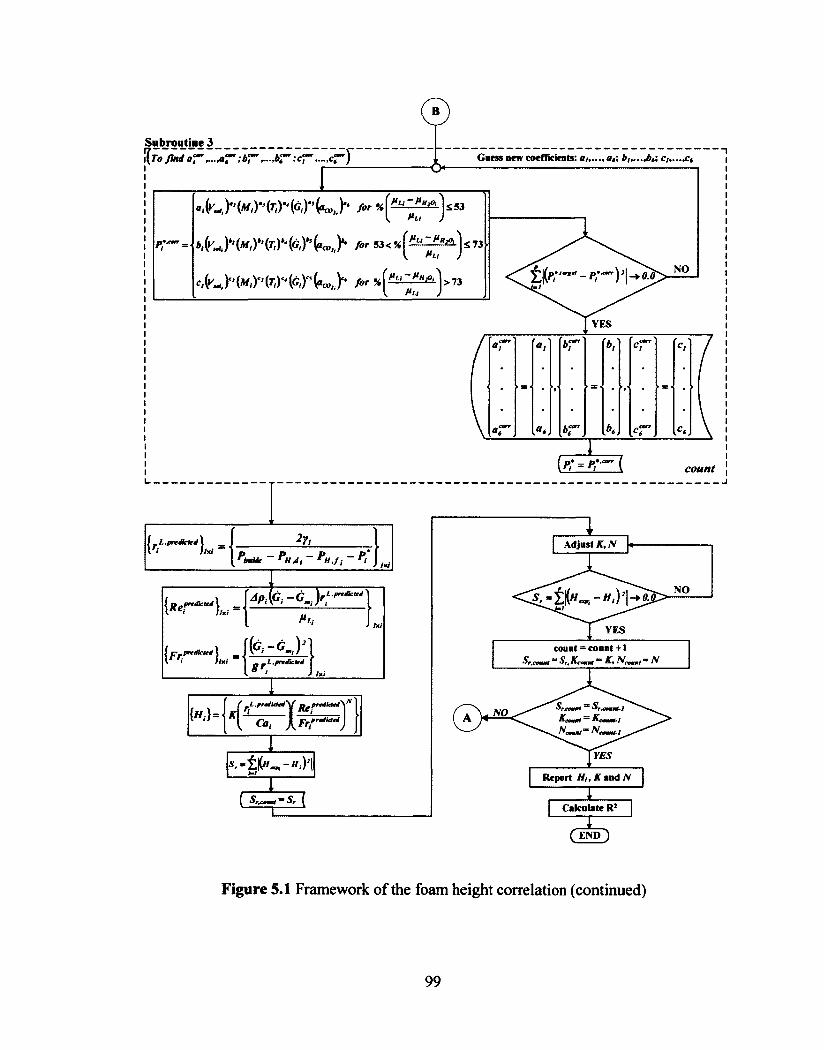
Subroutine 3 riTo ar ; br ,...,br ;cr
L
cri Guess new coefficients: al, 14; bb....b6;
al(v-i,)'(mirs(Tir'(014z60„) for % ( fli" /1" ) 53PLI
(aco,, )16 for 53 < 73
ci(Vm,)"(Mir(Ti)44 (6) " (aco4)`' for %(11" — P112°1ifr"" — P7') 21-. 0.0
( or
=1
a,
.
br
I, „ .
b,'
„
cr
ly . = .1
c„.
.
7
I
\ ar a6 bT b6 cr ,c6 \
count
27i {riL,prediried) =
I'd hd
P — PH ,d i — PH J i —
{dp. 6 —6 rL' 'dia`d} (Rerfw"),„ — ' ' '''')
'P
PL,
iFerediceedL i _1( — )2 g r L ,predicard
!xi
hti
{H,}={4e."1{Ref'll Ca, Fr/predtried
J.,
Cakulate R2
( END
Figure 5.1 Framework of the foam height correlation (continued)
99
Sabrontiiie3 {to find aT,...,ar ;bT ;CT cfT Guess new coefficients: a/,..., a,;
rt
-,(^,)C1 (*0" ft)" (6,)" for %(^"~^ ' ] > 7 3
*r
YES
1 count
L--2?/
L-Art k " /XJ
W^L -Jp , Gi-Cm,)rLp"acu'\ \ ' ml f I
W^L - L •fa--<U1 „ L,prtdkK<l [
.* 1 J /xi 3
I
I
Adjust AT, yv
count = count +1 S„Kc„m-K,N,
Report Hi, K and N T
Calculate R2
"7x— ( END )
Figure 5.1 Framework of the foam height correlation (continued)
99

5.2 Subroutine calculations
5.2.1 Average bubble radius
This work deals with the average radius of bubbles that wander between the gas
dispersion layer and gas-liquid interface because they are less deviated than those in the
foam layer, which are tremendously subject to disproportionation or Ostwald ripening.
The average bubble radius was determined under different experimental conditions using
the Laplace equation (Bikerman, 1973) shown in Equation (2.3) (page 35). The capillary
pressure is instantaneously created across any curved interface with two principal radii of
curvature (RI and R2) at a given point between gas and liquid phases or two immiscible
liquids due to surface tension. With an assumption of the spherical gas bubbles, both radii
are at the gas side and equal to the average bubble radius (RI = R2 = r) resulting in a
positive capillary pressure. Thus, Equation (2.3) (page 35) can be rewritten as follows:
r = 2y r
(5.1)
The positive capillary pressure in Equation (5.1) is the difference between the pressure
inside (or at the concaved side) of the gas bubble (P,„,,,,k) and the pressure outside (or at
the convex side) of the gas bubble (P„„,„de) as written below:
P c P inside P ouiside (5.2)
Since it is difficult to measure Pinside of the compressed gas at the diffuser, Pinstde
is assumed to be atmospheric even though in reality, Pinside is above atmospheric pressure
due to the compression of gas through the diffuser and P - outside is approximately
atmospheric. Regardless of the assumed Amide, Pc must remain positive. The average
bubble radius can be calculated by combining Equations (5.1) and (5.2) as shown below:
100
5.2 Subroutine calculations
5.2.1 Average bubble radius
This work deals with the average radius of bubbles that wander between the gas
dispersion layer and gas-liquid interface because they are less deviated than those in the
foam layer, which are tremendously subject to disproportionation or Ostwald ripening.
The average bubble radius was determined under different experimental conditions using
the Laplace equation (Bikerman, 1973) shown in Equation (2.3) (page 35). The capillary
pressure is instantaneously created across any curved interface with two principal radii of
curvature (Ri and R2) at a given point between gas and liquid phases or two immiscible
liquids due to surface tension. With an assumption of the spherical gas bubbles, both radii
are at the gas side and equal to the average bubble radius (R/ = R2 = r) resulting in a
positive capillary pressure. Thus, Equation (2.3) (page 35) can be rewritten as follows:
P.=— (5.1) r
The positive capillary pressure in Equation (5.1) is the difference between the pressure
inside (or at the concaved side) of the gas bubble (Pmide) and the pressure outside (or at
the convex side) of the gas bubble (Poutside) as written below:
Pe = f.Inside ~ ̂ outside (5.2)
Since it is difficult to measure Pinside of the compressed gas at the diffuser, PinSide
is assumed to be atmospheric even though in reality, PinSide is above atmospheric pressure
due to the compression of gas through the diffuser and Poutside is approximately
atmospheric. Regardless of the assumed Pinside, Pc must remain positive. The average
bubble radius can be calculated by combining Equations (5.1) and (5.2) as shown below:
100

2y r =
kP inside P outside)
(5.3)
When a gas bubble is detached from the diffuser, the bubble is immediately exposed to
the pressure in the test cell as demonstrated in Figure 5.2. The outside pressure of the
bubble is composed of the hydrostatic pressures caused by gas dispersion and foam layers
above the bubble. Although the Laplace equation was established to predict the bubble
radius for static rather than dynamic systems, this limitation can be corrected to reflect
the actual turbulent surroundings of the bubble by adding the additional pressure term
called P* to account for the stress caused by the flow of other bubbles, the pressure
caused by the incoming gas flow, and the normal pressure due to the collision between
bubbles. Therefore, the P outsde can be expressed as:
P outstde = PH ,d PH,f P
PH ,d = P LSO d)ild
,f. = P Lg(1 — f)H exp
(5.4)
(5.5)
(5.6)
where P fbd and PM! are the hydrostatic pressures due to the gas dispersion layer defined
via Equation (5.5) (N/m2) and the foam layer defined via Equation (5.6) (N/m2),
respectively. The calculation of other parameters is given below:
v. cell v L — , s0a,
Ed v. cell
L
Vr" hd =
100A
H exP 11)0
exP
O A
101
When a gas bubble is detached from the diffuser, the bubble is immediately exposed to
the pressure in the test cell as demonstrated in Figure 5.2. The outside pressure of the
bubble is composed of the hydrostatic pressures caused by gas dispersion and foam layers
above the bubble. Although the Laplace equation was established to predict the bubble
radius for static rather than dynamic systems, this limitation can be corrected to reflect
the actual turbulent surroundings of the bubble by adding the additional pressure term
called P* to account for the stress caused by the flow of other bubbles, the pressure
caused by the incoming gas flow, and the normal pressure due to the collision between
bubbles. Therefore, the Poutside can be expressed as:
where PN,D and PH,/ are the hydrostatic pressures due to the gas dispersion layer defined
via Equation (5.5) (N/m2) and the foam layer defined via Equation (5.6) (N/m2),
respectively. The calculation of other parameters is given below:
outside
(5.5)
(5.4)
(5.6)
yce l l _ y r L v sol (5.7)
cell
(5.8)
H — EXP exp 100 A
(5.9)
101

where ed is the gas fraction in the gas dispersion layer calculated using Equation (5.7), hd
is the height of the gas dispersion layer (m) calculated using Equation (5.8), Hew is the
experimental steady-state foam height (m), which is calculated from the experimental
steady-state foam volume (ve,p, cm3) shown in Equation (5.9), and ef is the gas fraction
in the foam layer, which is assumed to be equal to 0.75 (Watstra, 1989) from the
literature review summarized in the table in Figure 2.1 (page 33). This void fraction was
expected to represent a typical morphology of the foams observed during the static
experiments as shown in Figure 5.3, which was a combination of Kugelschaum and
Polyederschaum. Tiny gas bubbles were formed after N2 was dispersed through the
diffuser. These bubbles hit and sat at the interface to form Kugelschaum, which was
mainly composed of spherical bubbles. Then, Kugelschaum started to change to
Polyederschaum, wherein most of the spherical bubbles were deviated to the polyhedral
bubbles.
By substituting Equation (5.4) into Equation (5.3), the final relationship based on
the Laplace equation to predict r is expressed as
r= 2y
inside — PH ,d PH ,f — Ps(5.10)
where P* can be determined using the following empirical correlations, depending upon
surface viscosity. These P* correlations were obtained by regressing our experimental
data given in Chapter 4 with R2 of 0.96.
P* = 109925.52 T3.436x10-3 65.3840-7
v m
1.9240-2 1.50x10⁻³ 3.004 0-4r sat "*CO2
104410 06 ML93X1°-3 T6.83x10-3O4.64104
where %(PL — PH20 j < 53
PL (5.11)
u lA040-2 , 3.62x10⁻³ so /
where 53 < %(PL — PH20
73 (5.12) 4.4co, PL
102
where £d is the gas fraction in the gas dispersion layer calculated using Equation (5.7), hd
is the height of the gas dispersion layer (m) calculated using Equation (5.8), HEXP is the
experimental steady-state foam height (m), which is calculated from the experimental
steady-state foam volume (oexp, cm3) shown in Equation (5.9), and £/ is the gas fraction
in the foam layer, which is assumed to be equal to 0.75 (Watstra, 1989) from the
literature review summarized in the table in Figure 2.1 (page 33). This void fraction was
expected to represent a typical morphology of the foams observed during the static
experiments as shown in Figure 5.3, which was a combination of Kugelschaum and
Polyederschaum. Tiny gas bubbles were formed after N2 was dispersed through the
diffuser. These bubbles hit and sat at the interface to form Kugelschaum, which was
mainly composed of spherical bubbles. Then, Kugelschaum started to change to
Polyederschaum, wherein most of the spherical bubbles were deviated to the polyhedral
bubbles.
By substituting Equation (5.4) into Equation (5.3), the final relationship based on
the Laplace equation to predict r is expressed as
r = - ^^ (5.10) Y inside ~ PhM ~ PftJ ~ P )
where P* can be determined using the following empirical correlations, depending upon
surface viscosity. These P* correlations were obtained by regressing our experimental
data given in Chapter 4 with R2 of 0.96.
109925.52 r3 06x,r5G5-38xI0"7 . ^ jyi.92xio~2 wi.50xi<r' 3.ooxio-4 where ^
V sol m aCO, Hi. <53 (5.11)
IfM/M AA£ iyl.93xl0"3 7-6.83x10"' ^4.64x10^ (., ,, \ P- = 104410.06M T G ^ tH40x10-2 3.62X10"' y sol aC02 ML
<73 (5.12)
102

P. = 104167.39 1 1524°-47,2.50.10-3
69.61x10⁻² a l:01,10-3 where %(/4/.. PH20 > 73
PL (5.13)
where T is solution temperature (°C), M is MEA concentration (kmol/m3), V301 is solution
volume (cm3), a co2 is CO2 loading (mol CO2/mol MEA), G is in the unit of m/s for
Equations (5.11) — (5.13). The sensitivity of coefficients on 1)* are studied by varying
±10% from the reported values. Results in Table 5.1 indicate that the most sensitive
coefficients are the coefficients al, b1 and ci (see Figure 5.1, page 98). Note that the
average bubble radius calculated in this work ranged from 0.09 to 0.47 mm. This range is
in good agreement with the bubble radius (0.005-0.5 mm) indicated in ASTM D892,
which creates the gas dispersion layer beneath the foam layer (ASTM, 1999).
103
P' = 104167.39 M 39 A/3'52*10' 7,2-50xl°3
where %f^ ^2°1>73 (5.13) I VL J
9.61x10 /•l.31x10* sol
,1.01x10
CO,
where T is solution temperature (°C), M is MEA concentration (kmol/m3), Vso/ is solution
volume (cm3), aCOi is CO2 loading (mol C02/mol MEA), G is in the unit of m/s for
Equations (5.11) - (5.13). The sensitivity of coefficients on P* are studied by varying
±10% from the reported values. Results in Table 5.1 indicate that the most sensitive
coefficients are the coefficients ai, bj and c/ (see Figure 5.1, page 98). Note that the
average bubble radius calculated in this work ranged from 0.09 to 0.47 mm. This range is
in good agreement with the bubble radius (0.005-0.5 mm) indicated in ASTM D892,
which creates the gas dispersion layer beneath the foam layer (ASTM, 1999).
103

Table 5.1 Sensitivity analysis of coefficients used in the prediction of P'
Coefficien
t
% variation in P5
Prediction with coefficient +10% Prediction with coefficient - 10%
al - 10 10
a2 1 -1
a3 0.01 - 0.01
04 - 0.11 0.11
a5 4.06x10⁻⁵ - 4.06x10⁻⁵
a6 - 3.06x10⁻³ 3.06x10⁻³
b 1 - 10.00 10.00
b2 0.83 - 0.84
b3 - 0.03 0.03
b4 - 0.28 0.27
b5 0.03 - 0.03
b6 - 0.04 0.04
CI - 10.00 10.00
C2 7.54 - 8.16
C3 - 0.06 0.06
C4 - 0.10 0.10
C5 - 7.43 6.92
C6 - 0.01 0.01
104
Table 5.1 Sensitivity analysis of coefficients used in the prediction of P*
Coefflcien % variation in P*
t Prediction with coefficient +10% Prediction with coefficient - 10%
O] -10 10
02 1 -1
a3 0.01 -0.01
a4 -0.11 0.11
a.j 4.06x10⁻⁵ - 4.06x 10"5
C16 - 3.06x10³ 3.06x10"3
b, - 10.00 10.00
b2 0.83 -0.84
b3 -0.03 0.03
b4 -0.28 0.27
b5 0.03 -0.03
b6 -0.04 0.04
Cl -10.00 10.00
C2 7.54 -8.16
C3 -0.06 0.06
c4 -0.10 0.10
Cs -7.43 6.92
C6 -0.01 0.01
104
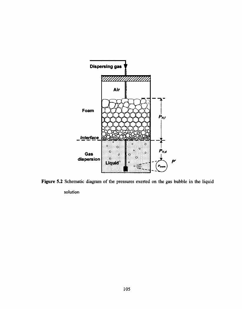
Dispersing gas
Gas dispersion P*
Figure 5.2 Schematic diagram of the pressures exerted on the gas bubble in the liquid
solution
105
Dispersing gas }
Foam
Interface
Gas dispersion
Air
M
* 0 0
tr 0
b °
Uqufd"
1
o-
• • : 1 3 . 0 , > - : 1
PH,f
PH,C
Figure 5.2 Schematic diagram of the pressures exerted on the gas bubble in the liquid
solution
105

Polyederschaum
Kugelschaum
Figure 5.3 Example of the foam observed in the static foaming experiment
(original in color)
Polyederschaum
Kugelschaum
Figure 53 Example of the foam observed in the static foaming experiment
(original in color)
106

5.2.2 Density
Since the nitrogen (N2) gas was assumed to follow the ideal gas law, the gas
density was calculated using the following equation:
P insicle(M N 2 ) G =
RT (5.14)
where pp is the density of N2 (kg/m3), Pi„,,d, is the pressure inside the gas bubble
(assumed to be equal to 101325 N/m2), R is the universal gas constant, MWN2 is the
molecular weight of N2, and T is the solution temperature (K).
The liquid density of the CO2-loaded aqueous MEA solutions at different CO2
loadings, MEA concentrations, and temperatures was estimated using the correlation
developed by Weiland and his team (Weiland et al., 1998):
[ X MEAMW MEA X H2OMW H 20 + X CO2 MW CO2
PL = 1000
V MEA =
X MEA VMEA li 2 0 + x V +xCO2 VCO2 +xMEA xH20 V* +xMEAXCO2 V ** 110
MW MEA
—5.35162x10⁻⁷ T2 —4.51417x10⁻⁴ T+1.19451
(5.15)
(5.16)
where PL is the density of the liquid solution (kg/m3); xi, MK, and V, are the mole
fraction, molecular weight, and molar volume (ml/mol), respectively, of MEA, water, and
CO2; T is the solution temperature (K); if is the constant equal to -1.8218; and V** is the
molar volume due to the interaction between MEA and CO2, which is equal to zero. The
standard deviation of the predicted value by the correlation is 0.00221.
107
5.2.2 Density
Since the nitrogen (N2) gas was assumed to follow the ideal gas law, the gas
density was calculated using the following equation:
Pc (5.14)
where pa is the density of N2 (kg/m3), P,„side is the pressure inside the gas bubble
(assumed to be equal to 101325 N/m ), R is the universal gas constant, MWNi is the
molecular weight of N2, and T is the solution temperature (K).
The liquid density of the C02-loaded aqueous MEA solutions at different CO2
loadings, MEA concentrations, and temperatures was estimated using the correlation
developed by Weiland and his team (Weiland et al., 1998):
pL =1000 X MEA M^mea + xh2o^Wh2o + xco2 M^co2
XMEA^MEA +XH,()VH20 + XC()2 K'O, + XMEAXH,0^ + XMEAXCoJ^ (5.15)
MW VMEA = r—. ^ J (5.16)
-5.35162x10 r -4.51417x10 T + 1.19451
where pi is the density of the liquid solution (kg/m3); jc„ MWh and V, are the mole
fraction, molecular weight, and molar volume (ml/mol), respectively, of MEA, water, and
CO2; T is the solution temperature (K); V* is the constant equal to -1.8218; and V*" is the
molar volume due to the interaction between MEA and CO2, which is equal to zero. The
standard deviation of the predicted value by the correlation is 0.00221.
107

5.2.3 Viscosity
The liquid viscosity (PL) of the CO2-loaded aqueous MEA solutions was
estimated using the following correlation developed by Weiland and his team (Weiland et
al., 1998):
L = x
PH20
}(21.186m + 2373) [aco, (0.01015m+ 0.0093T —2.2589)+ dm
T2 (5.17)
where pi, and 1111,0 are the viscosities of the aqueous MEA solution and water,
respectively (mPa s); m is the mass percent of MEA; and T is the solution temperature
(K). The standard deviation of the predicted value by the correlation is 0.0732.
5.2.4 Surface tension
Since the CO2-loaded aqueous MEA solutions were considered to be a tertiary
system, the work of Chunxi and his colleagues (Chunxi et al., 2000) was extended to
predict surface tension of the solutions using Gibbs free energy (G, J) needed to expand
per surface area (As, m2) at constant temperature (7), pressure (P), and composition i (x,),
as shown below:
Y-la 1,p,„
(5.18)
For a multi-component non-ideal solution under isothermal and isobaric conditions, the
molar Gibbs free energy of the bulk solution, which was assumed to be uniform across
the surface, was equal to the sum of the molar Gibbs free energy of the ideal solution
(G,dead, J) and the molar excess Gibbs free energy (G.„, J), which in this work was
predicted by the Wilson equation, as shown below:
108
5.23 Viscosity
The liquid viscosity (JIL) of the C02-loaded aqueous MEA solutions was
estimated using the following correlation developed by Weiland and his team (Weiland et
al., 1998):
(21.186/W+2373) [aCOi (0.01015m + 0.009371 - 2.2589)+l]m = exp<
Mh2O (5.17)
where Hi and //Wj0 are the viscosities of the aqueous MEA solution and water,
respectively (mPa s); m is the mass percent of MEA; and T is the solution temperature
(K). The standard deviation of the predicted value by the correlation is 0.0732.
5.2.4 Surface tension
Since the CC>2-loaded aqueous MEA solutions were considered to be a tertiary
system, the work of Chunxi and his colleagues (Chunxi et al., 2000) was extended to
predict surface tension of the solutions using Gibbs free energy (G, J) needed to expand
per surface area (As, m2) at constant temperature (7), pressure (P), and composition i (x,),
as shown below:
For a multi-component non-ideal solution under isothermal and isobaric conditions, the
molar Gibbs free energy of the bulk solution, which was assumed to be uniform across
the surface, was equal to the sum of the molar Gibbs free energy of the ideal solution
(fiideal* J) and the molar excess Gibbs free energy (Gexcess, J), which in this work was
predicted by the Wilson equation, as shown below:
108

G = G„kai + Gexcess (5.19)
G =(Ex,G,
v.
+ RT
— a
xiln xi j— RTExEln(ExiA y ) (5.20)
A = —v
exp (i~j) (5.21) RT
where ay is the constant representing the difference between interaction energy of
molecular pair ij (U) and that of molecular pair ii (U„) and v, and vv are the molar volume
of pure component i and j at constant temperature T (K), of which its ratio between two
components is equal to one (Chunxi et al., 2000). Therefore, the surface tension for the
multi-component system can be predicted by incorporating Equation (5.20) into Equation
(5.18) and differentiating it with respect to the surface area (A3), resulting in:
ia(u„, -u„)) y.E x,y, — RTE xe Ex. Exin, RT aAs ) T ,P
(5.22)
From Equation (5.22), there were two types of adjustable parameters: Uy — U„
accounting for the local composition effect and (a(Uy -u ,,)/ aAt,p, representing the
excess surface tension. Therefore, twelve adjustable parameters must be obtained for the
surface tension model (i.e., U12 - U11, U21 - U22, U13 - Ul 1, U3, - U33, U23 - U22,
U32 - U22, (a(U12 -U 11 )/ aA r (a(u2i -u22 )/air)T,p,x, (a(u,, - U ,,)/
(a(u3,-U33)/ (aW23-(122)/air),,p.„,, (a(u32- U 33 )/a4s),,,p,x,). Subscripts 1,
2, and 3 are MEA, CO2, and water, respectively. The twelve adjustable parameters were
minimized by assuming that the interaction of molecular pair ij (U,J) is equal to the
arithmetic average between those of the same molecular pair ii (U„) and jj (Un) (Chunxi
et al., 2000). As a result, six adjustable parameters remained for the correlation of surface
tension as listed below:
109
excess (5.19)
G = fZX'G' + RTYtX.lnx,]- RT^x. ln Y,xjAV \ i i J i \ j j
(5.20)
v , - a„ -^-exp—^ ( i*j) (5.21)
where ay is the constant representing the difference between interaction energy of
molecular pair ij (U,j) and that of molecular pair ii (£/,,) and v, and y, are the molar volume
of pure component i and j at constant temperature T (K), of which its ratio between two
components is equal to one (Chunxi et al., 2000). Therefore, the surface tension for the
multi-component system can be predicted by incorporating Equation (5.20) into Equation
(5.18) and differentiating it with respect to the surface area (As), resulting in:
From Equation (5.22), there were two types of adjustable parameters: Uy - U t i
excess surface tension. Therefore, twelve adjustable parameters must be obtained for the
surface tension model (i.e., Un - Uu, U21 - U22, U13 - (///, Ua - U33, U23 - U22,
u,2 - u2!, (a(ul2-u„)/dA-l(d(un-uI2)/8A-lJ,Ji,
(etUv-Uj/dA'l^, {stU^-U^/dA-l^, Subscripts 1,
2, and 3 are MEA, CO2, and water, respectively. The twelve adjustable parameters were
minimized by assuming that the interaction of molecular pair ij (Uy) is equal to the
arithmetic average between those of the same molecular pair ii (Uu) and jj ([Uy) (Chunxi
et al., 2000). As a result, six adjustable parameters remained for the correlation of surface
tension as listed below:
(5.22)
accounting for the local composition effect and (d(t/(/ - Un)/ dA s ̂ ^ representing the
109

U12 - U11 (U21 - U22)
U13 - Ull - (U31 - U33)
U23 - U22 = - (U32 - U22)
(a(u,2 —u11) a(u2 ( ,—u22))aAs aAs
(a(u13 —u11) (a(u3,—u33))aAs 0A3
49(U23 - U 22 )j o(u32 - U 33 )J
aAs aAs T ,P „xi
The final correlation of the surface tension is presented below:
y=1000
x,y, + x2 y2 + x3y3
— RT
ix ran,o+x (an,3 x, rx ran,,)+x ran 3 )) x2 A,2 +x3A,3 aAs ) aAs)) x,A 2,+x3A 2, 1 ) ads2 ))
x3 Cx1
ran21 + x,A3, +x2A32 aAs ) ,
(5.23)
(5.24)
(5.25)
(5.26)
(5.27)
(5.28)
(5.29)
In order to find the values of these parameters, a measurement of surface tension
for aqueous solutions of MEA containing CO2 was carried out experimentally by
applying the spinning drop method using a Spinning Drop Interfacial Tensiometer Model
510 (Temco, Inc, OK, USA). The experimental conditions and results of the
measurement were reported in Section 4.4 (Figure 4.7a, page 81). Multiple non-linear
regression with a stochastic technique was used to minimize the sum of squares of
residuals between the predicted surface tensions and the experimental ones. All the
correlation parameters needed for Equation (5.29) were determined and are given in
Table 5.2 with R2of 0.89.
110
U I2-U I I = -(U2 , -U22)
U I 3-U„ = -{U3 I-U3 3)
U2 3-U22=-(U32-U22)
(d(u„-uj (a(u2 , -uj)
I av , I ar J
ra(t/13-(/Mr| = . (3P„-Vn)) av ) T.Psi ar )r
%U*-UnY) (d(U,2
ar J T f j C j a4' J,
T.PJ,
(5.23)
(5.24)
(5.25)
(5.26)
(5.27)
(5.28) r.Pjj
The final correlation of the surface tension is presented below:
y = 1000
xj, +x2y2 +x3y }
x,
-RT Jf2A|2 +X3A,j
( f ao
+ AT, ' 3A | 3 Y|
V ) , dA' )) X,A2) +X}A2
8Aj, H dAs
+ x, dAy 8AS
*1^31 x2^-n + x2
\
l SA' J kdA' J /
(5.29)
In order to find the values of these parameters, a measurement of surface tension
for aqueous solutions of MEA containing CO2 was carried out experimentally by
applying the spinning drop method using a Spinning Drop Interfacial Tensiometer Model
510 (Temco, Inc, OK, USA). The experimental conditions and results of the
measurement were reported in Section 4.4 (Figure 4.7a, page 81). Multiple non-linear
regression with a stochastic technique was used to minimize the sum of squares of
residuals between the predicted surface tensions and the experimental ones. All the
correlation parameters needed for Equation (5.29) were determined and are given in
Table 5.2 with/^of 0.89.
110
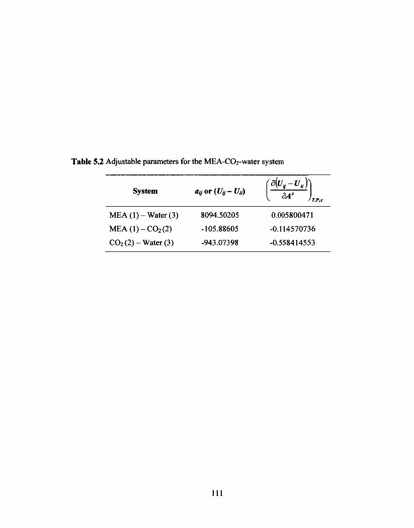
Table 5.2 Adjustable parameters for the MEA-0O2-water system
System aii or (14 — UN) (a(u,,—uil ))
aAs
MEA (1) — Water (3) 8094.50205 0.005800471
MEA (1) — CO2 (2) -105.88605 -0.114570736
CO2 (2) — Water (3) -943.07398 -0.558414553
Table 5.2 Adjustable parameters for the MEA-CCh-water system
System ay or (Uij - Ua) 3[v t-u„y
dA5 ' T,P,x
MEA (1) - Water (3)
MEA (1) - C02(2)
CO2 (2) - Water (3)
8094.50205
-105.88605
-943.07398
0.005800471
-0.114570736
-0.558414553
111

53 Foam height prediction results
With 134 experimental foaming data sets, an empirical correlation as shown
below and a series of subroutine modules for physical property estimation for the CO2-
loaded aqueous MEA system were successfully developed. The foam height correlation
comprises parameters including bubble radius, surface tension of liquid, viscosity of
liquid, difference in density of gas and liquid, and superficial gas velocity; constants K of
4394 and N of -1.30; and dimensionless Ca, Re, and Fr in ranges of 2.0x10⁻³ — 6.3x 10⁻²,
5.0 — 276.4, and 0.01 — 0.89, respectively. The summary of these dimensionless numbers
are given in Appendix B. The correlation fits well with the experimental data as indicated
by a R2 of 0.88 as illustrated in Figure 5.4. The detailed explanation for foaming
behaviour with respect to process parameters was previously given in Chapter 4 while the
discussions of correlation prediction are given below.
H = 4394 r • ir60
( . .30" G
V.30
I
(5.30)
112
S3 Foam height prediction results
With 134 experimental foaming data sets, an empirical correlation as shown
below and a series of subroutine modules for physical property estimation for the CO2-
loaded aqueous MEA system were successfully developed. The foam height correlation
comprises parameters including bubble radius, surface tension of liquid, viscosity of
liquid, difference in density of gas and liquid, and superficial gas velocity; constants K of
4394 and Nof-1.30; and dimensionless Ca, Re, and Fr in ranges of 2.0xl0"3 - 6.3xl0"2,
5.0 - 276.4, and 0.01 - 0.89, respectively. The summary of these dimensionless numbers
are given in Appendix B. The correlation fits well with the experimental data as indicated
by a R2 of 0.88 as illustrated in Figure 5.4. The detailed explanation for foaming
behaviour with respect to process parameters was previously given in Chapter 4 while the
discussions of correlation prediction are given below.
v /
(5.30)
112

0.0 10.0 20.0 30.0 40.0 50.0 60.0 Hem, (mm)
Figure 5.4 Parity chart between Hew and H for the foam height correlation (dashed lines
represent 95% confidence interval)
113
60.0
50.0
40.0
| 30.0
X 20.0
XX
10.0
0.0 0.0 10.0 20.0 30.0 40.0 50.0 60.0
Hexp(mm)
Figure 5.4 Parity chart between HEXP and //for the foam height correlation (dashed lines
represent 95% confidence interval)
113

The correlation can also describe the behaviour of foaming with changes in
process conditions. From Figure 5.5, the correlation gives good predictions compared to
the experimental data at the superficial gas velocity ranging from 0.12 to 0.94 mm/s. The
errors between the predicted foam heights and the experimental results are very small,
although a proportional increase in the experimental foam height with the superficial gas
velocity is only achieved at a certain range of the superficial gas velocity. As illustrated
in Figure 5.6, the experimental results show that the effect of the initial solution volume
on foam height is significant when the initial solution volume increases from 200 to 400
cm3 and becomes insignificant when the initial solution volume is greater than 400 cm3.
The predicted results show good agreement with the experimental data except for some
deviations observed at the minimum and maximum initial solution volumes. For this
correlation, the effect of initial solution volume is embedded in the calculation of the
average bubble radius through the prediction of P ju and P* instead of 6,„ , which can
implicitly account for this effect as previously discussed by Pilon et al. (2001). Thus,
incorporating 6„, into the correlation could possibly reduce these deviations. A further
development is required to explicitly recognize the initial solution volume as one of the
independent parameters in the future foam height correlation.
Figures 5.7 — 5.9 demonstrated that the correlation generally yields good
prediction of the foam height as the MEA concentration, CO2 loading, and solution
temperature are changed. However, a variation in the predicted and experimental foam
heights is noticeable at higher solution temperatures. Not only does the higher solution
temperature weaken the stability of foam by lowering liquid viscosity, but it also creates
a more severely turbulent environment caused by violent bubble movements, which can
disturb an existing foam layer. The latter can be observed from the experiment. Although
114
The correlation can also describe the behaviour of foaming with changes in
process conditions. From Figure 5.5, the correlation gives good predictions compared to
the experimental data at the superficial gas velocity ranging from 0.12 to 0.94 mm/s. The
errors between the predicted foam heights and the experimental results are very small,
although a proportional increase in the experimental foam height with the superficial gas
velocity is only achieved at a certain range of the superficial gas velocity. As illustrated
in Figure 5.6, the experimental results show that the effect of the initial solution volume
on foam height is significant when the initial solution volume increases from 200 to 400
cm and becomes insignificant when the initial solution volume is greater than 400 cm .
The predicted results show good agreement with the experimental data except for some
deviations observed at the minimum and maximum initial solution volumes. For this
correlation, the effect of initial solution volume is embedded in the calculation of the
average bubble radius through the prediction of PHJ and P* instead of Gm, which can
implicitly account for this effect as previously discussed by Pilon et al. (2001). Thus,
incorporating Gm into the correlation could possibly reduce these deviations. A further
development is required to explicitly recognize the initial solution volume as one of the
independent parameters in the future foam height correlation.
Figures 5.7 - 5.9 demonstrated that the correlation generally yields good
prediction of the foam height as the MEA concentration, C02 loading, and solution
temperature are changed. However, a variation in the predicted and experimental foam
heights is noticeable at higher solution temperatures. Not only does the higher solution
temperature weaken the stability of foam by lowering liquid viscosity, but it also creates
a more severely turbulent environment caused by violent bubble movements, which can
disturb an existing foam layer. The latter can be observed from the experiment. Although
114
the correlation uses Re to characterize the flow regimes, no proper Re criteria for
different flow regimes, to the best of our knowledge, has been provided for this particular
system. Then, it is possible that this particular correlation only works well in the laminar
and possibly transition regime. An additional parameter or another correlation for a
turbulent regime should be considered in future work.
115

70.0
60.0
E
0 40.0
E 30.0 0 u. 20.0
10.0
0.0 0.00 0.20 0.40 0.60 0.80
Superficial gas velocity(mm/s)
(a) 2.0 kmol/m3
70.0
60.0 •
E 50.0
a 40.0 - 0
30.0 - o IL 20.0 -
10.0 -
0.0 0.00 0.20 0.40 0.60 0.80
Superficial gas velocity(mm/s)
(b) 5.0 kmol/m3
Figure 5.5 Simulation results of predicted foam height with respect to superficial gas
velocity (solution volume = 400 cm3, CO2 loading = 0.40 mol/mol and
solution temperature = 40°C) with MEA concentration (a) 2.0 kmol/m3 and
(b) 5.0 kmol/m3
1.00
1.00
116
70.0
60.0
| 50.0
% 40.0 o
E 30.0 CO o "• 20.0
10.0
0.0
_ •
—•— Experiment
— P r e d i c t e d
0.00 0.20 0.40 0.60 0.80 Superficial gas velocity(mm/s)
(a) 2.0 kmol/m3
1.00
70.0
60.0
| 50.0
» 40.0
E 30.0 (0 o
20.0
10.0 Experiment
Predicted 0.0
0.00 1.00 0.20 0.40 0.60 0.80 Superficial gas velocity(mm/s)
(b) 5.0 kmol/m3
Figure 5.5 Simulation results of predicted foam height with respect to superficial gas
velocity (solution volume = 400 cm3, CO2 loading = 0.40 mol/mol and
solution temperature = 40°C) with MEA concentration (a) 2.0 kmol/m3 and
(b) 5.0 kmol/m3
116

40.0
30.0
I E .*.. f o 20.0 - m.-.
E 10 .0- L ..
0.0
.,. - - - "" • . ..
, 4c
Experiment
---x-- Predicted
0 •
200 400 600 Solution volume (cm3)
800
Figure 5.6 Simulation results of predicted foam height with respect to solution volume
(MEA concentration = 2.0 kmol/m3, superficial gas velocity = 0.57 mm/s,
CO2 loading = 0.40 mol/mol and solution temperature = 40°C)
117
40.0
30.0 -E E
I 20.0 -© JZ E to £ 10.0 -
—•— Experiment
—x— Predicted 0.0
0 200 400 600 800 Solution volume (cm3)
Figure 5.6 Simulation results of predicted foam height with respect to solution volume
(MEA concentration = 2.0 kmol/m3, superficial gas velocity = 0.57 mm/s,
CO2 loading = 0.40 mol/mol and solution temperature = 40°C)
117

40.0
-i- 30.0 -E . .c .:2: 20.0 -
i o IL 10.0 -
0.0
0.0
■ ■
--0— Experiment --a--- Predicted
2.0 4.0 6.0 MEA concentration (kmolim3)
(a) Absorber top
0.0 2.0 4.0 6.0 MEA concentration (kmoUm3)
(b) Absorber bottom
Figure 5.7 Simulation results of predicted foam height with respect to MEA
concentration (superficial gas velocity = 0.57 mm/s and solution volume =
400 cm3); (a) absorber top condition: CO2 loading = 0.20 mol/mol and
solution temperature = 40°C and (b) absorber bottom condition: CO2 loading
= 0.40 mol/mol and solution temperature = 60°C
8.0
8.0
118
—•— Experiment
Predicted
I 1 1 I 1 I * 2.0 4.0 6.0 8.0
MEA concentration (kmol/m3)
(a) Absorber top
? 30.0 E,
B) ® 20.0
E (0 o u.
10.0
0.0 0.0 2.0 4.0 6.0 8.0
MEA concentration (kmol/m3)
(b) Absorber bottom
Figure 5.7 Simulation results of predicted foam height with respect to MEA
concentration (superficial gas velocity = 0.57 mm/s and solution volume =
400 cm3); (a) absorber top condition: CO2 loading = 0.20 mol/mol and
solution temperature = 40°C and (b) absorber bottom condition: CO2 loading
= 0.40 mol/mol and solution temperature = 60°C
10.0 -
0.0 --0.0
1
•
—•— Experiment
— P r e d i c t e d I 1 1 1 I 1 I
118

50.0 E 40.0 -. .1.a. 30.0 - co 1 20.0 - i 10.0 -0
13. 0.0 0.00 0.10 0.20 0.30 0.40 0.50 0.60 CO2 loading in solution
(mol CO2/mol MEA)(a) 40°C
50.0 E 40.0 - .c 4- 30.0 - a' 'd 20.0 - i 10.0 -0 w 0.0
0.00 0.10 0.20 0.30 0.40 0.50 0.60 CO2 loading in solution (mol CO2/mol MEA)
(b) 60°C 50.0 ....... - E 40.0 -EFE-. 30.0 -
en -'m 20.0 - .c . i 10.0 - o 'LI' 0.0
0.00 0.10 0.20 0.30 0.40 0.50 0.60 CO2 loading in solution (mol CO2/mol MEA)
(c) 90°C
Figure 5.8 Simulation results of predicted foam height with respect to CO2 loading
(MEA concentration = 5.0 kmol/m3, superficial gas velocity = 0.57 mm/s and
solution volume = 400 cm3) with solution temperature (a) 40°C, (b) 60°C, and
(c) 90°C
119
® 20.0
i 10.0 o "" 0.0
— E x p e r i m e n t Predicted T 1 1 1 1 I 1 1 1 1 1—
0.00 0.10 0.20 0.30 0.40 0.50 0.60 COz loading in solution
(mol COJmol MEA)
(a) 40°C
50.0
1 40.0
2 30.0 o> | 20.0
i 10.0 o u. 0.0
9 % ir-i"
•» * xr — E x p e r i m e n t •» * xr
Predicted
0.00 0.10 0.20 0.30 0.40 0.50 0.60 COz loading in solution
(mol COj/mol MEA)
(b) 60°C
Expenment Predicted E 40.0
«- 30.0
3 20.0
§ 10.0
0.00 0.10 0.20 0.30 0.40 0.50 0.60 C02 loading in solution
(mol C02/mol MEA)
(c) 90°C
Figure 5.8 Simulation results of predicted foam height with respect to CO2 loading
(MEA concentration = 5.0 kmol/m3, superficial gas velocity = 0.57 mm/s and
solution volume = 400 cm3) with solution temperature (a) 40°C, (b) 60°C, and
(c) 90°C
119

0.0 40.0 50.0 60.0 70.0 80.0
Solution temperature (°C)
(a) 0.20 mol CO2/mol MEA
60.0
50.0 E
E-; 40.0 .c p) 2 30.0 -
Io u. 20.0 -
90.0
10.0 -
0.0 40.0
--s— Experiment
- - x- - - Predicted
--x
50.0 60.0 70.0 80.0 Solution temperature (°C)
90.0
(b) 0.40 mol CO2/mol MEA
Figure 5.9 Simulation results of predicted foam height with respect to solution
temperature (MEA concentration = 5.0 kmol/m3, superficial gas velocity =
0.57 mm/s and solution volume = 400 cm3) with CO2 loading (a) 0.20
mol/mol and (b) 0.40 mol/mol
120
60.0
_ 50.0 E E r 40.0 f JSP £ 30.0 E «o £ 20.0
10.0
0.0 40.0 50.0 60.0 70.0 80.0 90.0
Solution temperature (°C)
(a) 0.20 mol CCVmol MEA
60.0 -| —•— Experiment
50.0 1( Predicted E
§ 40.0 £ O) 1 30.0 E n £ 2 0 . 0 .
10.0
0.0 40.0 50.0 60.0 70.0 80.0 90.0
Solution temperature (°C)
(b) 0.40 mol CCVmol MEA
Figure 5.9 Simulation results of predicted foam height with respect to solution
temperature (MEA concentration = 5.0 kmol/m3, superficial gas velocity =
0.57 mm/s and solution volume = 400 cm3) with CO2 loading (a) 0.20
mol/mol and (b) 0.40 mol/mol
—•— Experiment
-Hi— Experiment
Predicted
120

5.3.1 Parametric effects
From Equation (5.30), the foam height is a function of bubble radius, difference
in density of gas and liquid, surface tension of liquid, viscosity of liquid, and superficial
gas velocity. The bubble radius has an inverse relationship with the foam height, which is
similar to the findings from Zhang and Fruehan (1995). That is, the foam height increases
with a decrease in the bubble radius due to an enhancement of foam stability. Very
minute bubbles with a spherical shape are much more stable than coarse bubbles with a
polyhedral shape. This is because the coarse bubbles are susceptible to bubble
coalescence, which causes bubble bursting. The density difference between gas and
liquid plays a role in foam height through foam drainage. The greater the density
difference, the lower the foam height. The increase in the density difference between gas
and liquid helps accelerate the velocity of liquid (u, mm/s) in the vertical lamella flowing
down from between the two parallel and immobile films with the thickness of 5 due to
the gravitational field to the bulk solution as expressed below (Bikerman, 1973):
„,s 2
= "I/ u12µ L
(5.31)
This deteriorates the stability of foam through drainage of liquid solution in the lamella to
the bulk solution. Note that since the gas density near atmospheric conditions is three
orders of magnitude smaller than the liquid density, the density difference between gas
and liquid is in this case mainly refers to the liquid density.
The surface tension affects the foam height in an inverse fashion as indicated by
the term 7/r16 of Equation (5.30) where r is proportional to y at a given capillary
pressure (Equation (5.3), page 101). A decrease in the surface tension causes the foam
height to rise because the minimum work required to expand the interface, or interfacial
121
5.3.1 Parametric effects
From Equation (5.30), the foam height is a function of bubble radius, difference
in density of gas and liquid, surface tension of liquid, viscosity of liquid, and superficial
gas velocity. The bubble radius has an inverse relationship with the foam height, which is
similar to the findings from Zhang and Fruehan (1995). That is, the foam height increases
with a decrease in the bubble radius due to an enhancement of foam stability. Very
minute bubbles with a spherical shape are much more stable than coarse bubbles with a
polyhedral shape. This is because the coarse bubbles are susceptible to bubble
coalescence, which causes bubble bursting. The density difference between gas and
liquid plays a role in foam height through foam drainage. The greater the density
difference, the lower the foam height. The increase in the density difference between gas
and liquid helps accelerate the velocity of liquid (u, mm/s) in the vertical lamella flowing
down from between the two parallel and immobile films with the thickness of 5 due to
the gravitational field to the bulk solution as expressed below (Bikerman, 1973):
u =Apgd_
12/i,
This deteriorates the stability of foam through drainage of liquid solution in the lamella to
the bulk solution. Note that since the gas density near atmospheric conditions is three
orders of magnitude smaller than the liquid density, the density difference between gas
and liquid is in this case mainly refers to the liquid density.
The surface tension affects the foam height in an inverse fashion as indicated by
the term /r16 of Equation (5.30) where r is proportional to y at a given capillary
pressure (Equation (5.3), page 101). A decrease in the surface tension causes the foam
height to rise because the minimum work required to expand the interface, or interfacial
121
free energy, is decreased, and consequently, foam formation is promoted. The surface
tension also plays a role in foam stability through the Marangoni effect occurring when
there is a difference between surface tension of the aqueous MEA solution and of the
CO2-loaded aqueous MEA solution. As the surface tension of the CO2-loaded aqueous
MEA solution decreases, the surface tension gradient is increased. The foam stability is,
thus, enhanced.
The solution viscosity affects the foam height in a proportional manner. An
increase in the solution viscosity increases the foam height due to an enhancement of
foam stability. As the solution viscosity increases, the liquid drainage from the lamella in
the foam layer to the bulk solution, owing to gravity drainage, is retarded, thereby
resulting in greater foam stability. This can be seen from the relationship between liquid
velocity and viscosity in Equation (5.31) (i.e. increasing the viscosity slows down the
liquid velocity). Note that the stability of foam could be destroyed if the surface viscosity
is so high that it causes immobile films between the lamella.
The superficial gas velocity influences the foam height (i.e. an increase in the
superficial gas velocity increases the foam height). This is a result of increasing volume
and number of bubbles generated in the system as shown in the following equation:
VGdiff = V= NbubVbubE (5.32)
where rt6d- ifir is the entire gas volume dispersed through the diffuser (m3) and Nfrub is the
number of the bubbles formed at the diffuser per a unit of time.
5.3.2 Sensitivity analysis
Sensitivity analysis was carried out to rank the parametric effects on the foam
height. Two types of parameters, dependent and independent, are involved in foaming in
122
free energy, is decreased, and consequently, foam formation is promoted. The surface
tension also plays a role in foam stability through the Marangoni effect occurring when
there is a difference between surface tension of the aqueous MEA solution and of the
CC>2-loaded aqueous MEA solution. As the surface tension of the CCh-loaded aqueous
MEA solution decreases, the surface tension gradient is increased. The foam stability is,
thus, enhanced.
The solution viscosity affects the foam height in a proportional manner. An
increase in the solution viscosity increases the foam height due to an enhancement of
foam stability. As the solution viscosity increases, the liquid drainage from the lamella in
the foam layer to the bulk solution, owing to gravity drainage, is retarded, thereby
resulting in greater foam stability. This can be seen from the relationship between liquid
velocity and viscosity in Equation (5.31) (i.e. increasing the viscosity slows down the
liquid velocity). Note that the stability of foam could be destroyed if the surface viscosity
is so high that it causes immobile films between the lamella.
The superficial gas velocity influences the foam height (i.e. an increase in the
superficial gas velocity increases the foam height). This is a result of increasing volume
and number of bubbles generated in the system as shown in the following equation:
V (f = v = Nb u bVb u hYJ (5.32)
where V (f f f is the entire gas volume dispersed through the diffuser (m3) and Nb u b is the
number of the bubbles formed at the diffuser per a unit of time.
5.3.2 Sensitivity analysis
Sensitivity analysis was carried out to rank the parametric effects on the foam
height. Two types of parameters, dependent and independent, are involved in foaming in
122

the CO2 absorption process. The independent parameters are process parameters (i.e.,
superficial gas velocity, solution volume, MEA concentration, CO2 loading, and solution
temperature). The dependent parameters are physical properties (i.e., gas density, liquid
density, liquid viscosity, and surface tension). To perform the sensitivity analysis, ranges
of these parameters were defined as listed in Tables 5.3 — 5.4. The minimum and
maximum values of the process parameters were adopted from the static experimental
conditions while those of the physical properties were determined from the subroutine
calculations (Sections 5.2.2 — 5.2.4) using the minimum and maximum values of the
process parameters. For each process parameter, a curve was plotted between percent
change in parameter and foam height index. The value of the parameter of interest was
increased in 10 percent increments from its minimum to its maximum while the rest of
the process parameters were fixed at either their minimum or maximum values. Note that
the values of the physical properties changed with respect to the increase in the given
process parameter. The foam height index is defined as a ratio of the predicted foam
height at a new value of a parameter to the predicted foam height at the minimum value
of a parameter. A similar procedure was applied to the sensitivity analysis of all of the
physical properties.
The results in Figures 5.10 — 5.11 show that the foam height increases with
superficial gas velocity, solution volume, CO2 loading, MEA concentration, gas density,
liquid density, and liquid viscosity but decreases with solution temperature and surface
tension. Among process parameters, solution volume is the most influential on the foam
height, followed by solution temperature. The remaining parameters, superficial gas
velocity, CO2 loading, and MEA concentration, have similar effects on the foam height.
The solution volume and superficial gas velocity mechanically affect foam height while
123
the CO2 absorption process. The independent parameters are process parameters (i.e.,
superficial gas velocity, solution volume, MEA concentration, CO2 loading, and solution
temperature). The dependent parameters are physical properties (i.e., gas density, liquid
density, liquid viscosity, and surface tension). To perform the sensitivity analysis, ranges
of these parameters were defined as listed in Tables 5.3 - 5.4. The minimum and
maximum values of the process parameters were adopted from the static experimental
conditions while those of the physical properties were determined from the subroutine
calculations (Sections 5.2.2 - 5.2.4) using the minimum and maximum values of the
process parameters. For each process parameter, a curve was plotted between percent
change in parameter and foam height index. The value of the parameter of interest was
increased in 10 percent increments from its minimum to its maximum while the rest of
the process parameters were fixed at either their minimum or maximum values. Note that
the values of the physical properties changed with respect to the increase in the given
process parameter. The foam height index is defined as a ratio of the predicted foam
height at a new value of a parameter to the predicted foam height at the minimum value
of a parameter. A similar procedure was applied to the sensitivity analysis of all of the
physical properties.
The results in Figures 5.10 - 5.11 show that the foam height increases with
superficial gas velocity, solution volume, CO2 loading, MEA concentration, gas density,
liquid density, and liquid viscosity but decreases with solution temperature and surface
tension. Among process parameters, solution volume is the most influential on the foam
height, followed by solution temperature. The remaining parameters, superficial gas
velocity, CO2 loading, and MEA concentration, have similar effects on the foam height.
The solution volume and superficial gas velocity mechanically affect foam height while
123

the rest of the process parameters impact the foam height through physical properties. A
change in solution temperature, CO2 loading, and MEA concentration primarily affects
liquid viscosity followed by liquid density, surface tension, and gas density as seen from
the relationships given in Sections 5.2.2 — 5.2.4. Among the physical properties (Figure
5.11), the foam height is the most sensitive to liquid viscosity, followed by liquid density
and surface tension, while it is not sensitive to gas density.
124
the rest of the process parameters impact the foam height through physical properties. A
change in solution temperature, CO2 loading, and MEA concentration primarily affects
liquid viscosity followed by liquid density, surface tension, and gas density as seen from
the relationships given in Sections 5.2.2 - 5.2.4. Among the physical properties (Figure
5.11), the foam height is the most sensitive to liquid viscosity, followed by liquid density
and surface tension, while it is not sensitive to gas density.
124

Table 5.3 Ranges of process parameters
Parameter Minimum Maximum
Superficial gas velocity (mm/s) 0.12 0.94
Solution volume (cm3) 200 700
MEA concentration (kmol/m3) 2.0 7.0
CO2 loading (mol/mol) 0.10 0.55
Solution temperature (°C) 40 90
125
Table 5.3 Ranges of process parameters
Parameter Minimum Maximum
Superficial gas velocity (mm/s) 0.12 0.94
Solution volume (cm3) 200 700
MEA concentration (kmol/m3) 2.0 7.0
CO2 loading (mol/mol) 0.10 0.55
Solution temperature (°C) 40 90
125

Table 5.4 Ranges of physical properties
Parameter Minimum Maximum
Gas density (kg/m3) 0.94 1.09
Liquid density (kg/m3) 976 1173
Liquid viscosity (mPas) 0.41 6.18
Surface tension (mN/m) 15.7 62.5
126
Table 5.4 Ranges of physical properties
Parameter Minimum Maximum
Gas density (kg/m3) 0.94 1.09
Liquid density (kg/m3) 976 1173
Liquid viscosity (mPa s) 0.41 6.18
Surface tension (mN/m) 15.7 62.5
126

.9 .c E
u.
Foa
m h
eig
ht i
ndex
8.00
7.00 -
6.00 -
5.00
4.00 -
3.00
2.00 -
1.00
0.00 0
8.00
7.00 -
6.00 -
5.00 -
4.00 -
3.00
2.00 -
1.00
0.00
-B-Superficial gas velocity - -x- • Solution volume
MEA concentration - CO2 loading - Solution temperature
•
,,•
••• • • -X'
10 20 30 40 50 60 70 80 90 100 %increase in parameter
(a)
-9- Superficial gas velocity - Solution volume ---*- MEA concentration -AD-• CO2 loading -4- Solution temperature
.-.". .• •
0 10 20 30 40 50 60 70 80 90 100 %increase in parameter
(b)
Figure 5.10 Sensitivity analysis of process parameters on foam height; (a) minimum
value of the remaining process parameters and (b) maximum value of the
remaining process parameters
127
8.00
7.00
$ 6.00 X3
Z 5.00 £ SP © 4.00 £
i 3.00 o u.
2.00
-e— Superficial gas velocity •-*-•• Solution volume
MEA concentration CO2 loading Solution temperature
,.;c
10 20 30 40 50 60 70 80 90 100 %increase in parameter
(a)
8.00
7.00 -
3 6.00 -"D Z 5.00 £ « 4.00 £
i 3.00 o
-b— Superficial gas velocity *- Solution volume
MEA concentration - CO2 loading -•*- Solution temperature
j:
x-
..-a'
0 10 20 30 40 50 60 70 80 90 100 %increase in parameter
(b)
Figure 5.10 Sensitivity analysis of process parameters on foam height; (a) minimum
value of the remaining process parameters and (b) maximum value of the
remaining process parameters
127

8.00
7.00
6.00
5.00 .2) • 4.00 E o 3.00 u.
2.00
1.00
0.00
8.00
7.00
6.00
:5 5.00 a) .c • 4.00 E 0 3.00 u.
2.00
1.00
0.00
0 10 20 30 40 50 60 70 80 90 100 %increase in parameter
(a)
-9- Gas density - -- - Liquid density
Liquid viscosity - •-• Surface tension
X.•
•
_ . _ . -g• •
0 10 20 30 40 50 60 70 80 90 100 %increase in parameter
(b)
Figure 5.11 Sensitivity analysis of physical properties on foam height; (a) minimum
value of the remaining process parameters and (b) maximum value of the
remaining process parameters
128
Gas density - -x- • Liquid density
Liquid viscosity Surface tension •o 6.00
5.00 IP ©
4.00 E o 3.00
I I 10 20 30 40 50 60 70 80
%increase in parameter 90 100
(a) 8.00
7.00 -x «
T3 C 6.00 -
£ 5.00 -O) 0 JZ 4.00 -£ (0 o 3.00 -u.
2.00 •
1.00
0.00
—a— Gas density - -x- - Liquid density —*•— Liquid viscosity —Surface tension
80 90 100
1 , 1 i 1 i r—
0 10 20 30 40 50 60 70 %increase in parameter
(b)
Figure 5.11 Sensitivity analysis of physical properties on foam height; (a) minimum
value of the remaining process parameters and (b) maximum value of the
remaining process parameters
128

6. DEVELOPMENT OF A FOAM MODEL
This chapter involves five main parts: i) development of a foam model for
columns fitted with the metal sheet structured packing as a column internal due to its
rising popularity in industrial use, high mass-transfer performance, and low pressure
drop; ii) generation of experimental foam data from a laboratory-scale absorber packed
with Mellapak 500.Y; iii) model verification with the experimental foam data; iv) model
simulation for foaming tendency; and v) evaluation of foaming impacts on process
performance.
6.1 Model development
A foam model for the alkanolamine-based CO2 absorption process using sheet-
metal structured packing as a column internal was developed with an aim to predict foam
volumes generated under a wide spectrum of CO2 absorption operation. The model was
built on the concept depicted in Figure 6.1. That is, a total foam volume generated within
a column is the sum of the foam volumes generated on all packing slabs when a packing
slab is defined as a half of the corrugation channel. Each slab has a number of
perforations and is partially covered by liquid rivulets. Only the perforations covered
with the liquid rivulets are considered to be foam sites accommodating foam formation as
they provide liquid pools for gas to disperse in. The foam volume at a given foam site is
quantified by using the pneumatic steady-state foam correlation (see Equation (5.30),
page 112). The total foam volume of a packing section is essentially a product of the
foam volume per one slab and the total number of slabs in the packing section. Based on
this concept, a model framework shown in Figure 6.2 was established to incorporate three
129
6. DEVELOPMENT OF A FOAM MODEL
This chapter involves five main parts: i ) development of a foam model for
columns fitted with the metal sheet structured packing as a column internal due to its
rising popularity in industrial use, high mass-transfer performance, and low pressure
drop; it) generation of experimental foam data from a laboratory-scale absorber packed
with Mellapak 500.Y; iii) model verification with the experimental foam data; iv) model
simulation for foaming tendency; and v) evaluation of foaming impacts on process
performance.
6.1 Model development
A foam model for the alkanolamine-based CO2 absorption process using sheet-
metal structured packing as a column internal was developed with an aim to predict foam
volumes generated under a wide spectrum of CO2 absorption operation. The model was
built on the concept depicted in Figure 6.1. That is, a total foam volume generated within
a column is the sum of the foam volumes generated on all packing slabs when a packing
slab is defined as a half of the corrugation channel. Each slab has a number of
perforations and is partially covered by liquid rivulets. Only the perforations covered
with the liquid rivulets are considered to be foam sites accommodating foam formation as
they provide liquid pools for gas to disperse in. The foam volume at a given foam site is
quantified by using the pneumatic steady-state foam correlation (see Equation (5.30),
page 112). The total foam volume of a packing section is essentially a product of the
foam volume per one slab and the total number of slabs in the packing section. Based on
this concept, a model framework shown in Figure 6.2 was established to incorporate three
129

components: 1) input of parameters, 2) a slab foam model, and 3) prediction of total foam
volume.
130
components: 1) input of parameters, 2) a slab foam model, and 3) prediction of total foam
volume.
130

Slab
Structured packing
r t 1 REPRESENTATION OF SLAB FOAM MODEL
‘ 1 i t
. .
Gas •' -' .,.. I _ , '
(Section A-A)
No of slab for a length of a given packing
section
I
FOAM
Liquid Rivulets (Wetted stir ace)
Pneumatic steady-state foaming experiment
Foam volume/Slab
Total foam volume
Figure 6.1 Concept of a foam model development
131
Slab Packing sheet
Structured packing
REPRESENTATION OF SLAB FOAM MODEL
Liquid Rivulets (Wetted surface)
Dry surface
Perforations
Dispersing g«
FOAM
Gas t (Section A-A)
Pneumatic steady-state foaming experiment
No. of slab for a length of a given packing
section Foam volume/Slab
Total foam volume
Figure 6.1 Concept of a foam model development
131

r
INPUT PARAMETER
r
Packing and column design parameter
• Corrugation base (2B) • Element height (hp) • Crimp height (h,881,) • Specific area (ap) • Diameter of Perforation hole (D8) • Perforation factor (fo p,) • Column diameter (Dc)
Process parameter
• Amine concentration (Al) • Superficial liquid velocity ( L) • CO2 loading (aco2) • Operating pressure (P) • Temperature of feed liquid (7) • Superficial gas velocity (G)
SLAB FOAM MODEL
Hydrodynamic feature
r • Liquid holdup (h') 4
• Fraction of wetted surface area (4ened)
Liquid height (h8q)
S
Physical property
• Gas density (pG) • Liquid density (PL) • Liquid viscosity (pL) • Surface tension (y) • Water viscosity (p,2„)
Force
• Buoyancy force (F8) • Kinetic force (FK) • Surface force (Fs) • Hydrostatic force (FR)
Average bubble radius (r)
4
Pneumatic foam height
Y Oy .30
H = 4.394 r 1 • 6°
130(40
Slab foam volume
t ) slab = h 7;erforation
(hp It„„„p
sin B)
4
r
No. of slab
The total number of the slab (Nr)
V Total foam volume
UT = l) slab. i
TOTAL FOAM VOLUME
Figure 6.2 Model framework to predict total foam volume in a structured packed
absorber
132
INPUT PARAMETER
SLAB FOAM MODEL
TOTAL FOAM VOLUME
The total number of the slab (AY)
No. of slab Total foam volume
slab, i
Packing and column design parameter
Corrugation base (2B) Element height (hp)
Crimp height (ha Specific area (ap) Diameter of Perforation hole (DH) Perforation factor {/perforation)
Column diameter (Dc)
Amine concentration ( M ) Superficial liquid velocity (L) C02 loading («r02) Operating pressure ( P ) Temperature of feed liquid (T) Superficial gas velocity (G)
Process parameter
Figure 6.2 Model framework to predict total foam volume in a structured packed
absorber
132

6.1.1 Input of parameters
Three types of parameters are involved in the model (i.e., process, packing, and
column design parameters). The process parameters refer to alkanolamine concentration,
superficial velocity of gas and liquid, CO2 loading of solution, operating pressure, and
feed liquid temperature. The packing parameters characterize configuration of structured
packings, as well as a fluid flow pattern within the column, while the column design
parameter involves the information on column diameter. By principle, the column is
packed with a series of structured packing elements, each of which can be rotated at a
specific angle ranging from zero to 90° with respect to the adjacent elements. As
illustrated in Figure 6.3, the structured packing element used for the model development
is of a sheet-metal type that is made of several thin corrugated metal sheets with
perforations with diameter (Dh), a crimp geometry of crimp height (h„,mp), and
corrugation base (2B) arranged alternately parallel to each other and at a fixed angle (a)
to the horizontal plane. The corrugation is composed of two inclined slabs with a slope of
0, which can be calculated from the crimp geometry of the packing to the adjacent sheet.
Specifically, our simulation used Mellapak 500.Y with 4.5 mm Dh, 6.53 mm hcrimp and
9.60 mm 2B as a case study. In gas absorption operations, gas travels upward from the
bottom to the top of the column, whereas liquid flows countercurrently downward in the
form of thin liquid films on the surface of the structured packing along corrugation
channels and packing intersections. When the packing elements are wetted by these
films, it is possible to observe a foam layer covering all the wetted packing surface and
flowing along with the liquid downward to the bottom of the column as shown in Figure
6.3b.
133
6.1.1 Input of parameters
Three types of parameters are involved in the model (i.e., process, packing, and
column design parameters). The process parameters refer to alkanolamine concentration,
superficial velocity of gas and liquid, CO2 loading of solution, operating pressure, and
feed liquid temperature. The packing parameters characterize configuration of structured
packings, as well as a fluid flow pattern within the column, while the column design
parameter involves the information on column diameter. By principle, the column is
packed with a series of structured packing elements, each of which can be rotated at a
specific angle ranging from zero to 90° with respect to the adjacent elements. As
illustrated in Figure 6.3, the structured packing element used for the model development
is of a sheet-metal type that is made of several thin corrugated metal sheets with
perforations with diameter (£)/,), a crimp geometry of crimp height {hcrimp), and
corrugation base (2B) arranged alternately parallel to each other and at a fixed angle (a)
to the horizontal plane. The corrugation is composed of two inclined slabs with a slope of
9, which can be calculated from the crimp geometry of the packing to the adjacent sheet.
Specifically, our simulation used Mellapak 500.Y with 4.5 mm A,, 6.53 mm hcrimp and
9.60 mm 2B as a case study. In gas absorption operations, gas travels upward from the
bottom to the top of the column, whereas liquid flows countercurrently downward in the
form of thin liquid films on the surface of the structured packing along corrugation
channels and packing intersections. When the packing elements are wetted by these
films, it is possible to observe a foam layer covering all the wetted packing surface and
flowing along with the liquid downward to the bottom of the column as shown in Figure
6.3b.
133
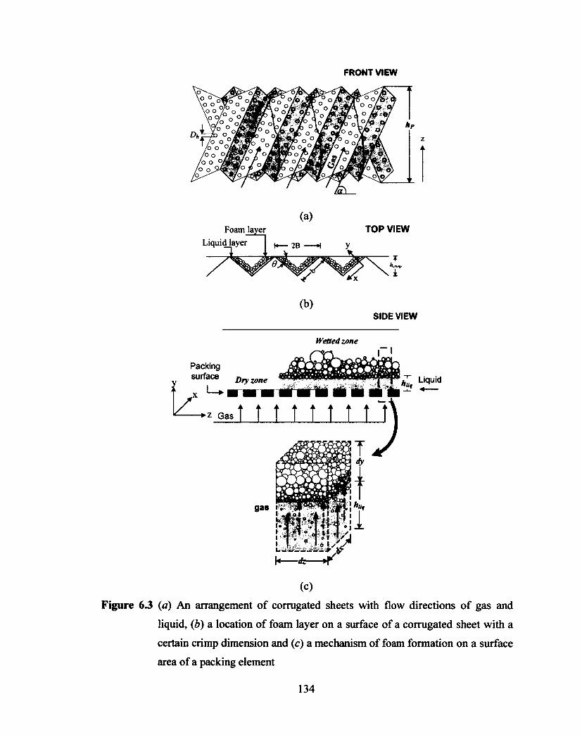
FRONT VIEW
Foam layer
Liquid layer
(a)
p4- 2B '"""" 11
•4(
(b)
TOP VIEW
SIDE VIEW
Wetted zone
Packing surface Dry zone
x iff-mg 111110111111111 IIII Ill III
>zGas1 T T rt
—
gas k
1
T dy
z
h' lig
Liquid
(c)
Figure 6.3 (a) An arrangement of corrugated sheets with flow directions of gas and
liquid, (b) a location of foam layer on a surface of a corrugated sheet with a
certain crimp dimension and (c) a mechanism of foam formation on a surface
area of a packing element
134
FRONT VIEW
(a) Foam layer TOP VIEW
Liquid layer 2B
V
(b)
T W
SIDE VIEW
Wetted zone
Packing surface Dry zone
z Gas
Liquid
(c) Figure 6.3 (a) An arrangement of corrugated sheets with flow directions of gas and
liquid, (b) a location of foam layer on a surface of a corrugated sheet with a
certain crimp dimension and (c) a mechanism of foam formation on a surface
area of a packing element
134

6.1.2 Slab foam model
A slab foam volume ( vsk,b) is the foam volume generated on one slab of the
corrugation channel. A liquid film with a thickness of hhq (Figure 6.3c) is divided into
small stationary volume elements, hi,q dxdz, through which both gas and liquid flow. Each
liquid volume element sufficiently accommodates an infinitesimal foam volume (dv) that
is generated when gas is dispersed underneath a given element and is expressed as:
dv = dxdydz (6.1)
where dx, dy, and dz are increments of distance in the x-axis, which is parallel to the
inclined packing surface; in the y-axis, which is perpendicular to the inclined packing
surface; and in the z-axis, which is parallel to the vertical, respectively. Since the foam
height only varies along the y-axis, the boundary conditions necessary for integrating
Equation (6.1) are listed below:
B.C. 1: at x = 0, = b hcrimp
(6.2) x =
sin 0
B.C. 2: at y = 0, y = H (6.3)
B.C. 3: at z = 0, z = hp (6.4)
where b is the slab width (m), H is the foam height formed on the surface of slab (m) and
hp is the height of a packing element (m), which in our simulation case, is equal to the
total height of the two Mellapak 500.Y packing elements. Therefore, the Vslab is a product
of the integration result of Equation (6.1) and the two factors, which are the liquid holdup
(h`) and the perforation factor (f v perforation) as given by:
(hp hcrimp slab
) v = h' f Peif°ramn H sin 0
(6.5)
135
6.1.2 Slab foam model
A slab foam volume (vsiab) is the foam volume generated on one slab of the
corrugation channel. A liquid film with a thickness of hi,g (Figure 6.3c) is divided into
small stationary volume elements, hnqdxdz, through which both gas and liquid flow. Each
liquid volume element sufficiently accommodates an infinitesimal foam volume (do) that
is generated when gas is dispersed underneath a given element and is expressed as:
dv = dxdydz (6.1)
where dx, dy, and dz are increments of distance in the x-axis, which is parallel to the
inclined packing surface; in the .y-axis, which is perpendicular to the inclined packing
surface; and in the z-axis, which is parallel to the vertical, respectively. Since the foam
height only varies along the j'-axis, the boundary conditions necessary for integrating
Equation (6.1) are listed below:
h, B.C.I: at x = 0, x = ft = -222. (6.2)
sin 9
B.C. 2: at ^ = 0, y = H (6.3)
B.C. 3: at z = 0, z = hp (6.4)
where b is the slab width (m), H is the foam height formed on the surface of slab (m) and
hp is the height of a packing element (m), which in our simulation case, is equal to the
total height of the two Mellapak 500.Y packing elements. Therefore, the vsiab is a product
of the integration result of Equation (6.1) and the two factors, which are the liquid holdup
(h') and the perforation factor if perforation) as given by:
®slab h fperforation ̂
f hP h
\
(6.5) sin 6 /
135

The liquid holdup represents the total amount of a liquid pool that accommodates
the onset of foaming, whereas the perforation factor indicates a fraction of an opening
hole on the surface area of the packing element where gas can flow upward through the
liquid pool. In the case of Mellapak 500.Y„fperforation is 0.102 with the distance between
the centers of two holes equal to 12.5 mm. H can be estimated from the foam height
correlation (see Equation (5.30), page 112) developed from the static foaming
experiments for the CO2 absorption process using aqueous alkanolamine solutions.
Details of the correlation and the prediction of physical properties were previously
discussed in Chapter 5.
From Equation (5.30) (page 112), the average radius of a gas bubble, a key
parameter in predicting the foam height, is calculated. As shown in Figure 6.4, the bubble
forms at a round perforation of the packing in which four forces (i.e., buoyancy force
(F8), kinetic force (FK), surface tension force (Fs), and hydrostatic force (FH)) play an
important role in the dimensions of the bubble. A balance equation of all forces is
expressed as:
FB FK = Fs + FH (6.6)
where the forces are in the unit of nN. r can be obtained by solving Equation (6.6).
Buoyancy and kinetic force are the upward forces that tend to disengage the bubble from
the perforation while surface tension and hydrostatic force act on the bubble in the
opposite direction. Buoyancy force is mainly caused by a density difference between gas
and liquid phases as shown below:
FB =-4 3 773 Apg (6.7)
136
The liquid holdup represents the total amount of a liquid pool that accommodates
the onset of foaming, whereas the perforation factor indicates a fraction of an opening
hole on the surface area of the packing element where gas can flow upward through the
liquid pool. In the case of Mellapak 500.Y, fperforation is 0.102 with the distance between
the centers of two holes equal to 12.5 mm. H can be estimated from the foam height
correlation (see Equation (5.30), page 112) developed from the static foaming
experiments for the CO2 absorption process using aqueous alkanolamine solutions.
Details of the correlation and the prediction of physical properties were previously
discussed in Chapter 5.
From Equation (5.30) (page 112), the average radius of a gas bubble, a key
parameter in predicting the foam height, is calculated. As shown in Figure 6.4, the bubble
forms at a round perforation of the packing in which four forces (i.e., buoyancy force
(FB), kinetic force (FK), surface tension force (Fs), and hydrostatic force (FH)) play an
important role in the dimensions of the bubble. A balance equation of all forces is
expressed as:
where the forces are in the unit of nN. r can be obtained by solving Equation (6.6).
Buoyancy and kinetic force are the upward forces that tend to disengage the bubble from
the perforation while surface tension and hydrostatic force act on the bubble in the
opposite direction. Buoyancy force is mainly caused by a density difference between gas
and liquid phases as shown below:
fb + = Fs + fH (6.6)
(6.7)
136

Kinetic force accounts for gas motion through a perforation with a diameter of Dh
(mm) as calculated by:
2 'FK = 500p,;62(1rD1 (6.8)
4
Surface tension force is the downward force produced by surface tension of liquid
phase exerting pressure on the perimeter of the hole as given below:
Fs = 70hy
1000 (6.9)
Hydrostatic force is the force pressing on the bubble when a certain amount of
liquid is present, which can be represented by:
pLghliy (47(7'2) FH (6.10)
1000
where hhq is the liquid height above the perforation hole (m) calculated by the following
equation:
h' hny =
fwelied a p
(6.11)
where ffemet is the fraction of the wetted surface area or, in this work, a ratio of the
effective mass-transfer area experimentally attained by Aroonwilas (2001) to the surface
area of the packing element; ap is the specific surface area (m2/m3 packing); and h' is the
liquid holdup at a given liquid velocity (m3 liquid solution/m3 packing) for Mellapak
estimated using the empirical equation with 10% accuracy (Suess and Spiegel, 1992), as
given below:
h' =capu3(0
\ 0.25 PL
PH20, 20*C (6.12)
137
Kinetic force accounts for gas motion through a perforation with a diameter of A,
(mm) as calculated by:
v 4 , (6.8) FK =500PGG2
Surface tension force is the downward force produced by surface tension of liquid
phase exerting pressure on the perimeter of the hole as given below:
F E£hV ( 69 ) s 1000
Hydrostatic force is the force pressing on the bubble when a certain amount of
liquid is present, which can be represented by:
p, ghlia 4w21 p 1 (6 1{))
" 1000
where hnq is the liquid height above the perforation hole (m) calculated by the following
equation:
K=-r— <61» J welted® P
where fwetted is the fraction of the wetted surface area or, in this work, a ratio of the
effective mass-transfer area experimentally attained by Aroonwilas (2001) to the surface
area of the packing element; ap is the specific surface area (m2/m3 packing); and ti is the
liquid holdup at a given liquid velocity (m3 liquid solution/m3 packing) for Mellapak
estimated using the empirical equation with 10% accuracy (Suess and Spiegel, 1992), as
given below:
/ \0.25
K = ca™(Lf CL
\^H20,20°C (6.12)
137

where L is the superficial liquid velocity (m3/m2-hr), jimio 20.c
is the water viscosity at
20°C (mPa's), c is 0.0169 for L < 40 m3/m2-hr or 0.0075 for L > 40 m3/m2-hr, and w is
0.37 for L < 40 m3/m2-hr or 0.59 for L > 40 m3/m2-hr.
138
where L is the superficial liquid velocity (m3/m2-hr), 20.c is the water viscosity at
20°C (mPa s), c is 0.0169 for L < 40 m3/m2-hr or 0.0075 for L> 40 m3/m2-hr, and w is
0.37 for L< 40 m3/m2-hr or 0.59 for L> 40 m3/m2-hr.
138

Hydrostatic force
IF Buoyancy Surface
force force
•
tKinetic force
Figure 6.4 Illustration of four main forces affecting average bubble radius
Hydrostatic force
1 Buoyancy Surface
force force
Gas
k Kinetic T force
Figure 6.4 Illustration of four main forces affecting average bubble radius
139

6.1.3 Prediction of total foam volume per packing section
In order to calculate the total foam volume after the vsiab is obtained, a number of
assumptions are applied to reduce mathematical complication. These are: 1) gas and
liquid countercurrently flows in the z-axis with a flow pattern of ideal plug flow
providing a uniform composition and flow rates, 2) perforations are distributed in a basic
regular pattern (Aroonwilas, 2001), 3) all foams after being generated on the packing
surface flow along the liquid stream to the bottom of the column without any collapse, 4)
only a variation of physical properties of both phases in the z-axis is considered, and 5)
the packing surface is wetted with the liquid to a thickness of hhq m, which is sufficient to
generate at least a monolayer of bubbles with an average bubble radius of r mm. With
these assumptions, the total foam volume ( v7-, m3) of the absorption column filled with a
series of structured packings is the sum of the slab foam volumes as expressed by:
41 4
UT = LUslab, i i=1
(6.13)
where NT is the total number of slabs per packing section of interest, which can be
determined by:
N = aA
b (6.14)
where A is the cross-sectional area of the column (m2). Note that the slab length is
assumed to be equal to the height of the given packing section.
140
6.1.3 Prediction of total foam volume per packing section
In order to calculate the total foam volume after the vsiab is obtained, a number of
assumptions are applied to reduce mathematical complication. These are: 1) gas and
liquid countercurrently flows in the z-axis with a flow pattern of ideal plug flow
providing a uniform composition and flow rates, 2) perforations are distributed in a basic
regular pattern (Aroonwilas, 2001), 3) all foams after being generated on the packing
surface flow along the liquid stream to the bottom of the column without any collapse, 4)
only a variation of physical properties of both phases in the z-axis is considered, and 5)
the packing surface is wetted with the liquid to a thickness of huq m, which is sufficient to
generate at least a monolayer of bubbles with an average bubble radius of r mm. With
these assumptions, the total foam volume (or, m3) of the absorption column filled with a
series of structured packings is the sum of the slab foam volumes as expressed by:
where Nr is the total number of slabs per packing section of interest, which can be
determined by:
where A is the cross-sectional area of the column (m2). Note that the slab length is
assumed to be equal to the height of the given packing section.
(6.13) 1=1
(6.14)
140

6.2 Results and discussions
6.2.1 Experimental foam data
The experimental foam data were analyzed and presented in Figure 6.5a (see
Appendix C) as a function of superficial liquid velocity and superficial gas velocity.
Results show that superficial liquid velocity has an apparent effect on foam volume,
whereas superficial gas velocity has a negligible effect at a low superficial liquid velocity
and a small effect at higher superficial liquid velocities. An increase in the superficial
liquid velocity generally increases foam volume generated at a given superficial gas
velocity. This can be explained by the fact that greater superficial liquid velocity lead to
greater degrees of wetted packing area and liquid holdup. As a result, the total number of
the perforations covered by the liquid solution is increased, which in turn increases
foaming tendency.
The negligible effect of superficial gas velocity is evident at the low superficial
liquid velocity of 0.8 m3/m2-hr (i.e., the foam volume does not change with superficial
gas velocity). This might be because the liquid holdup is too small to provide an adequate
liquid layer above the perforation hole or a sufficient contacting time between a gas
bubble and a liquid layer. However, at higher superficial liquid velocities, the foam
volume tends to increase with superficial gas velocity at a given superficial liquid
velocity. This is due to an increase in gas volume and in turn an increase in the number of
bubbles generated above the perforation holes.
It should be noted that at 360 nun/s superficial gas velocity for 2.3 m3/m2-hr
superficial liquid velocity and at 300 and 360 minis for a 3.1 m3/m2-hr, the turbulence
between gas and liquid phases at the bottom of absorber could create a slight drop in the
foam volumes. The turbulence, as shown in Figure 6.6, could even hinder the
141
6.2 Results and discussions
6.2.1 Experimental foam data
The experimental foam data were analyzed and presented in Figure 6.5a (see
Appendix C) as a function of superficial liquid velocity and superficial gas velocity.
Results show that superficial liquid velocity has an apparent effect on foam volume,
whereas superficial gas velocity has a negligible effect at a low superficial liquid velocity
and a small effect at higher superficial liquid velocities. An increase in the superficial
liquid velocity generally increases foam volume generated at a given superficial gas
velocity. This can be explained by the fact that greater superficial liquid velocity lead to
greater degrees of wetted packing area and liquid holdup. As a result, the total number of
the perforations covered by the liquid solution is increased, which in turn increases
foaming tendency.
The negligible effect of superficial gas velocity is evident at the low superficial
liquid velocity of 0.8 m3/m2-hr (i.e., the foam volume does not change with superficial
gas velocity). This might be because the liquid holdup is too small to provide an adequate
liquid layer above the perforation hole or a sufficient contacting time between a gas
bubble and a liquid layer. However, at higher superficial liquid velocities, the foam
volume tends to increase with superficial gas velocity at a given superficial liquid
velocity. This is due to an increase in gas volume and in turn an increase in the number of
bubbles generated above the perforation holes.
It should be noted that at 360 mm/s superficial gas velocity for 2.3 m3/m2-hr
superficial liquid velocity and at 300 and 360 mm/s for a 3.1 m3/m2-hr, the turbulence
between gas and liquid phases at the bottom of absorber could create a slight drop in the
foam volumes. The turbulence, as shown in Figure 6.6, could even hinder the
141
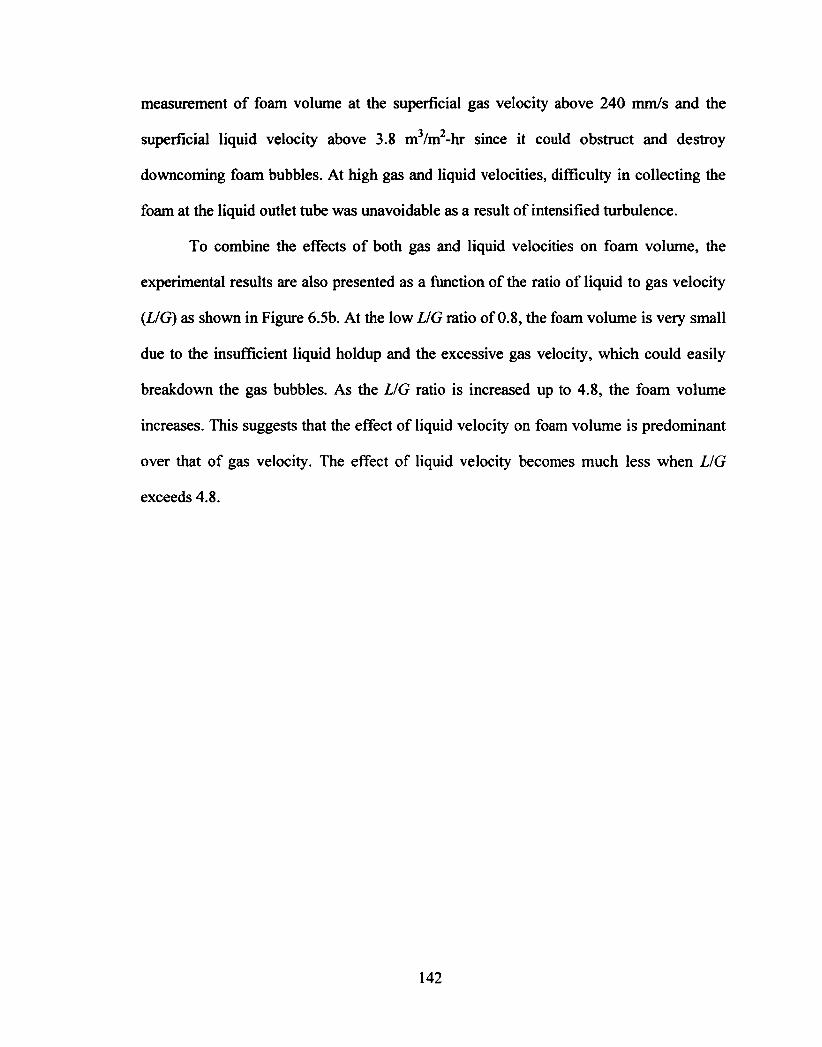
measurement of foam volume at the superficial gas velocity above 240 mm/s and the
superficial liquid velocity above 3.8 m3/m2-hr since it could obstruct and destroy
downcoming foam bubbles. At high gas and liquid velocities, difficulty in collecting the
foam at the liquid outlet tube was unavoidable as a result of intensified turbulence.
To combine the effects of both gas and liquid velocities on foam volume, the
experimental results are also presented as a function of the ratio of liquid to gas velocity
(LIG) as shown in Figure 6.5b. At the low LIG ratio of 0.8, the foam volume is very small
due to the insufficient liquid holdup and the excessive gas velocity, which could easily
breakdown the gas bubbles. As the LIG ratio is increased up to 4.8, the foam volume
increases. This suggests that the effect of liquid velocity on foam volume is predominant
over that of gas velocity. The effect of liquid velocity becomes much less when LIG
exceeds 4.8.
142
measurement of foam volume at the superficial gas velocity above 240 mm/s and the
superficial liquid velocity above 3.8 m /m -hr since it could obstruct and destroy
downcoming foam bubbles. At high gas and liquid velocities, difficulty in collecting the
foam at the liquid outlet tube was unavoidable as a result of intensified turbulence.
To combine the effects of both gas and liquid velocities on foam volume, the
experimental results are also presented as a function of the ratio of liquid to gas velocity
(L/G) as shown in Figure 6.5b. At the low LIG ratio of 0.8, the foam volume is very small
due to the insufficient liquid holdup and the excessive gas velocity, which could easily
breakdown the gas bubbles. As the LIG ratio is increased up to 4.8, the foam volume
increases. This suggests that the effect of liquid velocity on foam volume is predominant
over that of gas velocity. The effect of liquid velocity becomes much less when LIG
exceeds 4.8.
142

0.70
0.60 -
a. 0.60 - • 0EE oa 0.40 - > > E °' 0.30- a c o 32
c.) c a m 0.20 - P. a 0.10 -
0.00
• •
- = 0.8 m3/m2-hr -e-- L =1.5 m3/m2-hr -0- L = 2.3 m3/m2-hr - = 3.1 m3/m2-hr - 0- L = 3.8 m3/m2-hr
L = 4.6 m3/m2-hr
[ I I I
0 50 100 150 200 250 300 350 400 450 Superficial gas velocity (mm/s)
0.70
0.60 • a. O 0.50 - E E o 0 0.40 - > >
2 E
T • c 0.30 -
o c O a 0.20 -e 0 a. 0.10 -
0.00 0.00 5.00
(a)
10.00 UG
15.00 20.00
(b)
Figure 6.5 (a) Experimental percent foam volume per packing volume plotted versus the
superficial gas velocity at different superficial liquid velocities (MEA
concentration = 5.0 kmol/m3, CO2 loading = 0.40 mol/mol, and solution
temperature = 18.5°C) and (b) experimental foam volume per packing volume
plotted versus the LIG ratio (MEA concentration = 5.0 kmol/m3, CO2 loading
= 0.40 mol/mol, and solution temperature = 18.5°C)
143
o ex.
0.70
0.60
0.50
§1 If0-40
I c 0.30
Z o c CO « Q-o
0.20 -
CL 0.10 -
0.00
L = 0.8 m3/m2-hr L -1.5 m3/m2-hr L = 2.3 m3/m24ir L = 3.1 m3/m2-hr L = 3.8 m3/m2-hr L = 4.6 m3/m2-hr
50 100 150 200 250 300 350 400 450 Superficial gas velocity (mm/s)
(a)
ii s i E o> « c
~ 2 c S o Q. e O Q.
0.70
0.60
0.50
0.40
0.30
0.20
0.10
0.00 0.00 5.00 10.00
L/G 15.00 20.00
(b)
Figure 6.5 (a) Experimental percent foam volume per packing volume plotted versus the
superficial gas velocity at different superficial liquid velocities (MEA
concentration = 5.0 kmol/m3, CO2 loading = 0.40 mol/mol, and solution
temperature = 18.5°C) and (b) experimental foam volume per packing volume
plotted versus the LIG ratio (MEA concentration = 5.0 kmol/m3, CO2 loading
= 0.40 mol/mol, and solution temperature = 18.5°C)
143

Figure 6.6 Example of turbulence developed at the bottom of the column (superficial
liquid velocity = 2.3 m3/m2-hr and superficial gas velocity = 360 mm/s)
(original in color)
144
Figure 6.6 Example of turbulence developed at the bottom of the column (superficial
liquid velocity = 2.3 m3/m2-hr and superficial gas velocity = 360 mm/s)
(original in color)
144

6.2.2 Model verification
The developed foam model was verified with 67 experimental foam data sets in
Section 6.2.1. Results indicate that the model has a capacity to predict foam volume
within the absorber packed with sheet-metal structured packing with 16.3%AAD and
percent deviation of ±30%, as illustrated in the parity plot in Figure 6.7. The deviation of
the predicted foam volume could be caused by: 1) estimation of physical properties and
liquid holdup from available correlations that are intrinsic to certain degrees of deviation,
2) extrapolation of effective wetted area at the low superficial liquid velocity, 3)
approximation of total number of the corrugation channels, 4) estimation of average
bubble radius from theory and not from experimental measurements, and 5) violation of
model assumptions due to the nature of foam and column hydrodynamics (i.e., zero foam
collapse and zero liquid buildup between the packing elements). For the assumption of
zero foam collapse, a non-wetted surface area inside the packing element could create
blockage of foam bubbles from travelling down to the bottom. As a result, these bubbles
may build up, potentially coalesce into a large bubble, and eventually rupture.
Turbulence between gas and liquid phase above the liquid outlet, especially at high
velocities, could also be a factor in the destruction of downcoming bubbles. For the
assumption of zero liquid buildup between the packing elements, additional liquid
volume could be accumulated between the packings when packing elements are stacked
with a certain degree of rotation with respect to one another (Aroonwilas, 2001).
145

0.70
E 0.60 - = o > (A 0.50 - E § 6 1:5 0.40 - .2 > ..... ce .c 0.30 - 2 11
" 0. 0.20 -am •Cj a 0.10 - -a E o. 0.00
0.00
- a --a P--.-
O L = 0.8 m3/m2-hr .--" a L =1.5 m3/m2-hr
o L = 2.3 m3/m2-hr x 1= 3.1 m3/m2-hr & L= 3.8 m3/m2-hr • L = 4.6 m3/m2-hr
0.10 0.20 0.30 0.40 0.50 0.60 0.70 Experimental percent foam volume
per packing volume
Figure 6.7 Simulation results compared between the experimental and predicted percent
foam volume per packing volume
146
t
o
i c W ® .£ O J* in •o *-{& s 0.
0.70
0.60
0.50
0.40
0.30
0.20
0.10
0.00
A +30% ,aD
-30%
X 4-'
a o • o
X
A •
L = 0.8 m3/m2-hr L= 1.5 m3/m2-hr /Is 2.3 m3/m2-hr L = 3.1 m3/m2-hr L = 3.8 m3/m2-hr L = 4.6 m3/m2-hr
0.00 0.10 0.20 0.30 0.40 0.50 0.60 Experimental percent foam volume
per packing volume
0.70
Figure 6.7 Simulation results compared between the experimental and predicted percent
foam volume per packing volume
146

6.3 Model simulation
6.3.1 Foaming tendency within an absorber
To demonstrate an application of the developed foam model, the model was used
to predict foaming tendency of the MEA solution within an absorber with an inside
diameter of 0.10 m and packed with Mellapak 500.Y as a case study. The information of
operating conditions along the column height was obtained from Aroonwilas (2001). The
simulation results in Figure 6.8 show that the model has the capacity to predict local
foam volumes at different heights of the absorber where solution temperature and CO2
loading in the solution (or gas-phase CO2 concentration) are varied. The local foam
volume tends to be higher at the absorber top than at the bottom. This is mainly because
the system temperature at the absorber top is lower than that at the absorber's bottom,
reflecting a higher liquid viscosity at the absorber top, which retards the gravity drainage
of the liquid in lamella and in turn enhances the stability of foam.
It should be noted here that while the temperature plays a role in the foaming
tendency within the absorber as described previously, the CO2 loading of solution also
influences the foaming tendency but to a relatively small extent and in the opposite
manner. That is, as the solution travels downward, the CO2 loading increases. This alone
would result in a higher foam volume at the absorber bottom. However, the influence of
temperature on the foaming tendency predominates over that of CO2 loading, as
evidenced in Figure 6.8; thus, the higher foam volume is found at the absorber top, not at
the bottom.
147

0.70
0.60
r, o. 0.50 E• m0 .24.. 0.40
I 51- --#---- ----12> 0 i
go 0.30 - • 0.35 moUrnol @ L = 3.8 m3/m2-hr .2 3g.6. 0 0.45 moUmol @ L = 3.8 m3/m2-hr c 0 0.20 - O a • 0.35 mol/mol @ 1 = 7.6 m3/m2-hr
m 0 0 0.45 moUmol @ L = 7.6 m3/m2-hr
.10 a A 0.35 moUmol @ L = 12.2 m3/m2-hr
A 0.45 mollmol @ L = 12.2 m3/m2-hr 0.00
0.00
0.70
0.60 a. 0 a, 0.50 S• 1- .2 E = 0.40 - 0 - O o > Et E co 0.30 - 0 c .42 -Ng 4,4 0 c 0 0.20 - O a 2 a. O 0.10 -
0.00 0.00
0.50 1.00 1.50 Distance from the top (m)
(a)
-------o- __________ 0 -o-
2.00
A
• 20.7°C @ L = 3.8 m3/m2-hr o 50.2°C @ L = 3.8 m3/m2-hr • 21.5°C @ L = 7.6 m3/m2-hr o 44.7°C @ L = 7.6 m3/m2-hr • 21.1°C @ L = 12.2 m3/m2-hr A 33.7°C @ L = 12.2 m3/m2-hr
0.50 1.00 1.50 Distance from the top (m)
2.00
(b)
Figure 6.8 Simulated profiles of local foam volumes along the absorber height under various CO2 absorption conditions: (a) effect of CO2 loading of feed solution at three different superficial liquid velocities (feed solution temperature =
33.2 ± 1.1°C, air flow rate = 38.5 kmol/m2-hr and MEA concentration = 3.0
kmol/m3) and (b) effect of the temperature of feed solution at three different superficial liquid velocities (CO2 loading of feed solution = 0.33 mol/mol, air flow rate = 38.5 lcmoUm2-hr, and MEA concentration = 3.0 kmol/m3)
148
Q.
II 11 « C £3 +* o C (0 d> CL H a> Q.
0.70 -
0.60 1 4
0.50 i P*- 1 " t ,
— K . —t
-
0.40 j w
0.30 - • 0.35 mol/mol @ L = 3.8 m3/m2-hr
0.20 -• 0.45 mol/mol @ L = 3.8 m3/m2-hr
0.20 - • 0.35 mol/mol @ L = 7.6 m3/m2-hr
0.10 -0 0.45 mol/mol @ L - 7.6 m3/m2-hr
0.10 - A 0.35 mol/mol @ L =12.2 m3/m2-hr
0.00 A 0.45 mol/mol @ L =12.2 m3/m2-hr
1 1 » 1 » *
0.00 0.50 1.00 1.50 Distance from the top (m)
(a)
•
o A A
-B-20.7°C 50.2 °C 21.5°C 44.7 °C 21.1°C 33.7°C = 12.2
m3/m2-hr m3/m2-hr m3/m2-hr m3/m2-hr m3/m2-hr m3/m2-hr
2.00
0.00 0.50 1.00 1.50 2.00 Distance from the top (m)
(b)
Figure 6.8 Simulated profiles of local foam volumes along the absorber height under
various CO2 absorption conditions: (a) effect of CO2 loading of feed solution at three different superficial liquid velocities (feed solution temperature =
33.2 ± 1.1°C, air flow rate = 38.5 kmol/m2-hr and MEA concentration = 3.0
kmol/m3) and (b) effect of the temperature of feed solution at three different
superficial liquid velocities (CO2 loading of feed solution = 0.33 mol/mol, air
flow rate = 38.5 kmol/m2-hr, and MEA concentration = 3.0 kmol/m3)
148

The developed model was further used to evaluate the foaming tendency of the
degraded MEA solution containing a corrosion inhibitor under the experimental
conditions in Section 6.3.1 as a case study. Ammonium thiosulfate and sodium
metavadate were chosen as representatives for the degradation product and the corrosion
inhibitor, respectively, due to their ability for foam induction. According to our previous
study, ammonium thiosulfate enhances the foaming coefficient of the non-degraded and
uninhibited MEA solution by a factor of 1.23 while sodium metavadate enhances the
coefficient by 1.28. For the purpose of this evaluation, ammonium thiosulfate and sodium
metavadate were assumed to contribute no synergistic effect on the foaming tendency of
the MEA solution containing both of these chemicals. This means that the foaming
coefficient in the MEA containing ammonium thiosulfate and sodium metavadate was
estimated to be 1.51, which was the sum of the coefficient enhancement factors of these
chemicals. The simulated foam profiles along the absorber of this degraded and inhibited
MEA solution are given in Figure 6.9.
149

1.80
1.60
le) 1.40 a . Em 1.20
i a E
too > o > E im 0.80 4 U C
I. E i 0 AO "C 4 V
8 a0.40 .. 0 0- 020
0.00 r ,
7 - - - , _ ., .. __ 4 k.... .... " . ... _ . ... . .._. . . . . _ • ....,_,_.,__,__.41• _.___.._.. ._......
'
. - . . . , ,_ , 1 i k r ,
--e— non-degraded soin --1,-- degraded soin (deg.prod.) —*-- degraded soin (deg.prod. + corr. inhibitor
0.00 0.50 1.00 1.50 2.00 Distance from the top (m)
Figure 6.9 Effect of the degradation product (ammonium thiosulfate) and corrosion
inhibitor (sodium metavanadate) on the simulated foaming profile along the
absorber (air flow rate = 38.5 kmol/m2-hr, MEA concentration = 3.0
kmol/m3, CO2 loading of feed solution = 0.33 mol/mol, superficial liquid
velocity = 12.2 m3/m2-hr, and feed solution temperature = 21.1°C
(Aroonwilas, 2001)
150
1.80
1.60
fc 1-40
| « 1.20
jf 1.00
E o> 0.80 ' (V C J
£ ? 0.60 -C «8 g 0.40 o Q- 0.20 ^
0.00 0.00
non-degraded soln degraded soln (deg.prod.) degraded soln (deg.prod. + corr. inhibitor)
I ' ' I ' I ' ' I ' 1 } I T '"T - f1" •""T""' "T - "T' - 'I
0.50 1.00 1.50 Distance from the top (m)
2.00
Figure 6.9 Effect of the degradation product (ammonium thiosulfate) and corrosion
inhibitor (sodium metavanadate) on the simulated foaming profile along the
absorber (air flow rate = 38.5 kmol/m -hr, MEA concentration = 3.0
kmol/m , CO2 loading of feed solution = 0.33 mol/mol, superficial liquid
velocity = 12.2 m3/m2-hr, and feed solution temperature = 21.1°C
(Aroonwilas, 2001)
150

6.3.2 Foaming impact on process throughput
In addition to foaming tendency within the absorber, the developed model can
also be used to evaluate the impact of foaming on process throughput. As illustrated in
Figure 6.3b (page 134), the opening space of the corrugation channel is reduced as a
result of foam formation on the packing surface. This could lead to a decrease in
available void space for gas to flow through. Consequently, a reduction in volumetric
flow rate of gas stream is required to maintain a designed gas velocity (i.e. 1 m/s). This is
especially true for the existing plants where column diameter cannot be altered. On the
contrary, in the case of the new plants, such foaming impact can be minimized by
increasing the column diameter to a certain extent to maintain the process throughput.
To evaluate this impact, foam volume and process throughput under the process
conditions listed in Table 6.1 for the MEA solutions were determined using the
developed model. Results in Figure 6.10 show that the gas flow rate of the foaming
system is not significantly reduced (less than 2.1%) from that of the non-foaming system
at any given liquid velocity. This is because the foam volume generated is very small and
decreases the available void space by less than 2.1% from that of the non-foaming
system. However, the gas flow rates of the degraded and inhibited MEA solutions are
slightly reduced from that of the MEA solution containing no degradation product and
corrosion inhibitor. This suggests that the presence of degradation product and corrosion
inhibitor could further reduce the process throughput during foaming.
151
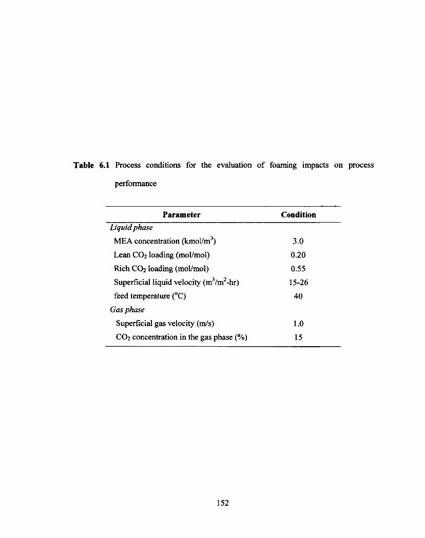
Table 6.1 Process conditions for the evaluation of foaming impacts on process
performance
Parameter Condition
Liquid phase
MEA concentration (kmol/m3) 3.0
Lean CO2 loading (mol/mol) 0.20
Rich CO2 loading (mol/mol) 0.55
Superficial liquid velocity (m3/m2-hr) 15-26
feed temperature (°C) 40
Gas phase
Superficial gas velocity (m/s) 1.0
CO2 concentration in the gas phase (%) 15
152
Table 6.1 Process conditions for the evaluation of foaming impacts on process
performance
Parameter Condition
Liquid phase
ME A concentration (kmol/m3) 3.0
Lean CO2 loading (mol/mol) 0.20
Rich CO2 loading (mol/mol) 0.55
Superficial liquid velocity (m3/m2-hr) 15-26
feed temperature (°C) 40
Gas phase
Superficial gas velocity (m/s) 1.0
CO2 concentration in the gas phase (%) 15
152

7.0E-03
1€7 I E
6.5E-03
O cf) 6.0E-03
E
o 5.5E-03 U)ea 0
5.0E-03
10.0
—o— non-foaming system
--4c— • foaming system (non-degraded soln)
foaming system (degraded soln. - deg.prod.)
El— foaming system (degraded soln. - deg.prod. + corr. inhibitor)
20.0 Superficial liquid velocity (m3/m2-hr)
30.0
Figure 6.10 Effect of the foaming on the gas volumetric flow rate for non-degraded and
degraded MEA solutions containing degradation product (ammonium
thiosulfate) and corrosion inhibitor (sodium metavanadate) (MEA
concentration = 3.0 kmol/m3, lean and rich CO2 loading of the solution =
0.20 and 0.55 mol/mol, respectively, feed solution temperature = 40°C, and
CO2 concentration in the gas phase = 15%)
153
7.0E-03
to
E "T 6.5E-03 s & I ® 6.0E-03 B o> | o 5.5E-03 > CO a O
5.0E-03 10.0 20.0 30.0
Superficial liquid velocity (m3/m2-hr)
Figure 6.10 Effect of the foaming on the gas volumetric flow rate for non-degraded and
degraded MEA solutions containing degradation product (ammonium
thiosulfate) and corrosion inhibitor (sodium metavanadate) (MEA
concentration = 3.0 kmol/m3, lean and rich CO2 loading of the solution =
0.20 and 0.55 mol/mol, respectively, feed solution temperature = 40°C, and
CO2 concentration in the gas phase = 15%)
—o— non-foaming system
- *- - foaming system (non-degraded soln)
foaming system (degraded soln. - deg.prod.)
- cd- - foaming system (degraded soln. - deg.prod. + corr. inhibitor)
1 I 1
153

7. CONCLUSIONS AND RECOMMENDATIONS
7.1 Conclusions
7.1.1 Parametric study
Results from the parametric study conducted in the static foaming experiment
allow useful conclusions on the effects of process parameters influencing the foaming
behaviour in alkanolamine-based CO2 absorption processes, which are drawn as follows:
• Solution volume affects foaming tendency when it is small. Increasing the solution
volume results in a constant foam volume or foaminess coefficient. After a certain
degree of increase, a plateau in foam volume or foaminess coefficient is reached.
• An increase in superficial gas velocity decreases foaminess coefficient. The gas
superficial gas velocity can lead to a constant foaminess coefficient when increased.
In other words, as above, after a certain degree of increase, a plateau is reached in
foaminess coefficient.
• Ranges of solution volume and superficial gas velocity that lead to a constant
foaminess coefficient were found for the CO2-aqueous alkanolamines. These ranges,
when used for foaming tests, enable the generation of foam data that are not
dependent on solution volume, gas flow rate, pore size of gas disperser, and
dimensions and volume of the test cell.
• Variations in MEA concentration, CO2 loading, and solution temperature affect
foaming tendency. Solution temperature is the most influential. An increase in
temperature decreases foaminess coefficient. The foaminess coefficient increases and
then declines with increasing MEA concentration and CO2 loading.
154
7. CONCLUSIONS AND RECOMMENDATIONS
7.1 Conclusions
7.1.1 Parametric study
Results from the parametric study conducted in the static foaming experiment
allow useful conclusions on the effects of process parameters influencing the foaming
behaviour in alkanolamine-based CO2 absorption processes, which are drawn as follows:
• Solution volume affects foaming tendency when it is small. Increasing the solution
volume results in a constant foam volume or foaminess coefficient. After a certain
degree of increase, a plateau in foam volume or foaminess coefficient is reached.
• An increase in superficial gas velocity decreases foaminess coefficient. The gas
superficial gas velocity can lead to a constant foaminess coefficient when increased.
In other words, as above, after a certain degree of increase, a plateau is reached in
foaminess coefficient.
• Ranges of solution volume and superficial gas velocity that lead to a constant
foaminess coefficient were found for the CC>2-aqueous alkanolamines. These ranges,
when used for foaming tests, enable the generation of foam data that are not
dependent on solution volume, gas flow rate, pore size of gas disperser, and
dimensions and volume of the test cell.
• Variations in ME A concentration, CO2 loading, and solution temperature affect
foaming tendency. Solution temperature is the most influential. An increase in
temperature decreases foaminess coefficient. The foaminess coefficient increases and
then declines with increasing MEA concentration and CO2 loading.
154

• Most degradation products and corrosion inhibitors in aqueous MEA solutions
enhance foaminess coefficient, except for sulfuric acid.
• MEA, MDEA, and MEA+AMP (2:1 mixing mole ratio) generate apparent foams
while DEA, AMP, MEA+MDEA, DEA+MDEA, and MEA+AMP (1:1 and 1:2) do
not.
• Physical properties, particularly surface tension, density, and viscosity of solution,
play a significant role in foaming tendency through foam formation and foam
stability.
7.1.2 Pneumatic foam height correlation
The empirical correlation for predicting pneumatic steady-state foam heights
generated in the CO2 absorption process using aqueous MEA solutions and a series of
subroutine modules for physical property estimation was successfully developed. The
foam height correlation was built on the Pilon et al. (2001) model with constants K and N
equalling 4394 and -1.30, respectively, and dimensionless Ca, Re, and Fr in the ranges of
2.0x 10⁻³ - 6.3x 10⁻², 5.0 — 276.4, and 0.01 — 0.89, respectively. The calculations involve
numerical iteration and statistical analysis, namely multiple non-linear regression with a
stochastic technique, as well as a series of subroutine modules for the estimation of
average bubble radius and physical properties. The findings are summarized as follows:
• The correlation fits well with the experimental foam data with R2 of 0.88. Most of the
predicted foam heights are in a good agreement with the experimental results within
the 95% confidence interval and can also predict the foaming tendency of the
solutions as the process conditions are varied.
155
• Most degradation products and corrosion inhibitors in aqueous MEA solutions
enhance foaminess coefficient, except for sulfuric acid.
• MEA, MDEA, and MEA+AMP (2:1 mixing mole ratio) generate apparent foams
while DEA, AMP, MEA+MDEA, DEA+MDEA, and MEA+AMP (1:1 and 1:2) do
not.
• Physical properties, particularly surface tension, density, and viscosity of solution,
play a significant role in foaming tendency through foam formation and foam
stability.
7.1.2 Pneumatic foam height correlation
The empirical correlation for predicting pneumatic steady-state foam heights
generated in the CO2 absorption process using aqueous MEA solutions and a series of
subroutine modules for physical property estimation was successfully developed. The
foam height correlation was built on the Pilon et al. (2001) model with constants K and N
equalling 4394 and -1.30, respectively, and dimensionless Ca, Re, and Fr in the ranges of
2.0xl0"3 - 6.3xl0"2, 5.0 - 276.4, and 0.01 - 0.89, respectively. The calculations involve
numerical iteration and statistical analysis, namely multiple non-linear regression with a
stochastic technique, as well as a series of subroutine modules for the estimation of
average bubble radius and physical properties. The findings are summarized as follows:
• The correlation fits well with the experimental foam data with R2 of 0.88. Most of the
predicted foam heights are in a good agreement with the experimental results within
the 95% confidence interval and can also predict the foaming tendency of the
solutions as the process conditions are varied.
155
• The correlation shows that the foam height inversely depends on the bubble radius, the
difference between the liquid and gas densities, and the surface tension but
proportionally depends on the viscosity and the superficial gas velocity.
• From the sensitivity analysis, the predicted foam height increases with superficial gas
velocity, solution volume, CO2 loading, MEA concentration, gas density, liquid
density, and liquid viscosity but decreases with solution temperature and surface
tension. Compared to other process parameters, solution volume is the most influential
on foam height, followed by solution temperature, and among physical properties,
foam height is the most sensitive to liquid viscosity, followed by liquid density and
surface tension, but it is not sensitive to gas density.
7.1.3 Foam model
A foam model for the alkanolamine-based CO2 absorption process was
successfully developed and verified with the experimental foaming data obtained from a
0.10 m (ID.) absorption column fitted with Mellapak 500.Y. Experimental results show
that superficial liquid velocity has an apparent effect on foam volume, whereas
superficial gas velocity has a negligible effect at a low liquid velocity and a small effect
at higher liquid velocities. The model has the capacity to predict foam volumes within the
absorber with an AAD of 16.3% and to determine local foam volumes at different
locations within a column packed with structured packing, which can be used to evaluate
foaming tendency and process throughput of the column and particularly the absorber.
The simulation results show that foaming is likely to occur more at the absorber top than
the bottom and causes no significant reduction in process throughput. However, during
actual plant operation, one can anticipate more foam volumes within the process due to
156

the presence of suspended solids and surfactant-based additives in the solutions, which
were not accounted for in this work.
7.2 Recommendations for future work
• Effect of solution volume and type of dispersing gas
For a pneumatic foam height correlation, the solution volume should be explicitly
included in the correlation as the independent parameter, as discussed in Chapter 5, since
it affects the terminal velocity of bubbles reaching the interface to form a foam layer.
Another improvement in the prediction is to account for the effect of gas type by
incorporating other physical properties of gas, besides the gas density, such as diffusion
coefficient and Oswald coefficient or solubility of gas in the liquid phase in future
correlations. Since the proposed correlation in this work was built on a set of foam
heights that were generated by one gas (i.e. N2) and no research has been conducted to
investigate the effect of the gas type on the foam height for this particular aqueous
solution, this limits the opportunity to examine foaming phenomena that can be affected
by the type of gas, such as, disproportionation. Hartland et al. (1993) studied the effect of
gases (i.e., xenon, nitrous oxide, N2 and CO2) used to bubble an aqueous solution of
10%wt glycerinate with the addition of Marlophen 89 on the foam height. They
discovered that the foam layer dispersed by gas with a higher gas solubility tended to be
more susceptible to collapse than that by gas with a lower gas solubility since the
interbubble gas diffusion or so-called disproportionation was much more pronounced at a
higher degree of solubility. This consequently led to poorer foam stability as a result of
faster growth in large bubbles or, in the other words, a more rapid decrease in the
interfacial area per unit gas volume (Hartland et al., 1993).
157
the presence of suspended solids and surfactant-based additives in the solutions, which
were not accounted for in this work.
7.2 Recommendations for future work
• Effect of solution volume and type of dispersing gas
For a pneumatic foam height correlation, the solution volume should be explicitly
included in the correlation as the independent parameter, as discussed in Chapter 5, since
it affects the terminal velocity of bubbles reaching the interface to form a foam layer.
Another improvement in the prediction is to account for the effect of gas type by
incorporating other physical properties of gas, besides the gas density, such as diffusion
coefficient and Oswald coefficient or solubility of gas in the liquid phase in future
correlations. Since the proposed correlation in this work was built on a set of foam
heights that were generated by one gas (i.e. N2) and no research has been conducted to
investigate the effect of the gas type on the foam height for this particular aqueous
solution, this limits the opportunity to examine foaming phenomena that can be affected
by the type of gas, such as, disproportionation. Hartland et al. (1993) studied the effect of
gases (i.e., xenon, nitrous oxide, N2 and CO2) used to bubble an aqueous solution of
10%wt glycerinate with the addition of Marlophen 89 on the foam height. They
discovered that the foam layer dispersed by gas with a higher gas solubility tended to be
more susceptible to collapse than that by gas with a lower gas solubility since the
interbubble gas diffusion or so-called disproportionation was much more pronounced at a
higher degree of solubility. This consequently led to poorer foam stability as a result of
faster growth in large bubbles or, in the other words, a more rapid decrease in the
interfacial area per unit gas volume (Hartland et al., 1993).

• Measurements of physical properties and average bubble radius
The model accuracy can be augmented by measuring physical properties and
average bubble radius rather than predicting and reducing model assumptions to account
for the complexity of the system. Measurements of physical properties of the solutions
are expected to enhance the accuracy of prediction. In particular, it is necessary to
measure both the equilibrium and dynamic surface tension of the CO2-loaded aqueous
solutions of alkanolamine, which are among the crucial liquid properties for foam
mechanisms, since no open literature has been published containing the information
regarding these surface tension measurements to date. Not only would this information
help predict foam height more accurately, but it is also expected to give a more in-depth
explanation of the foaming behaviour in this CO2 absorption process.
• Effects of suspended solids and surfactant-based additives
Suspended solids are considered one of the important factors and, based on plant
experience, are commonly found in the alkanolamine-based gas absorption process, being
introduced through either external or internal sources (Ballard, 1966, Lieberman, 1980,
Keaton and Bourke, 1983, Pauley et al., 1989). Iron sulphide (FeS) is recommended as an
example of the suspended solids to test the effect of suspended solids since it can be
formed in the circulating alkanolamine system through corrosion. Results from this work
can help establish the relationship between corrosion and foaming problems, which
would help practitioners to predict the onset of foam in the system more effectively. In
addition, the effect of surfactant-based additives, including corrosion inhibitors and
antifoam agents, should be examined to expand the application of the model.
158
• Measurements of physical properties and average bubble radius
The model accuracy can be augmented by measuring physical properties and
average bubble radius rather than predicting and reducing model assumptions to account
for the complexity of the system. Measurements of physical properties of the solutions
are expected to enhance the accuracy of prediction. In particular, it is necessary to
measure both the equilibrium and dynamic surface tension of the C02-loaded aqueous
solutions of alkanolamine, which are among the crucial liquid properties for foam
mechanisms, since no open literature has been published containing the information
regarding these surface tension measurements to date. Not only would this information
help predict foam height more accurately, but it is also expected to give a more in-depth
explanation of the foaming behaviour in this CO2 absorption process.
• Effects of suspended solids and surfactant-based additives
Suspended solids are considered one of the important factors and, based on plant
experience, are commonly found in the alkanolamine-based gas absorption process, being
introduced through either external or internal sources (Ballard, 1966, Lieberman, 1980,
Keaton and Bourke, 1983, Pauley et al., 1989). Iron sulphide (FeS) is recommended as an
example of the suspended solids to test the effect of suspended solids since it can be
formed in the circulating alkanolamine system through corrosion. Results from this work
can help establish the relationship between corrosion and foaming problems, which
would help practitioners to predict the onset of foam in the system more effectively. In
addition, the effect of surfactant-based additives, including corrosion inhibitors and
antifoam agents, should be examined to expand the application of the model.
158

8. REFERENCES
Abdi, M. A; Golkar, M. M.; Meisen, A. Improve Contaminant Control in Amine Systems. Hydrocarbon Processing. 2001, 80(10), 102C -102I.
Adamson, A. W. Physical Chemistry of Surfaces. 2nd ed.; John Wiley & Sons, Inc.: New York, 1967.
Aguila-Hernandez, J.; Trejo, A.; Garcia-Flores, B. E. Surface Tension and Foam Behaviour of Aqueous Solutions of Blends of Three Alkanolamines, As a Function of Temperature Colloids and Surfaces A: Physicochemical and Engineering Aspects. 2007, 308(1-3), 33 - 46.
Alvarez, E.; Rendo, R.; Sanjurjo, B.; Sanchez-Vilas, M.; Navaza, J. M. Surface Tension of Binary Mixtures of Water + N-Methyldiethanolamine and Tertiary Mixtures of this Amine and Water with Monoethanolamine, Diethanolamine, and 2-Amino-2-methyl- 1 -propanol from 25 to 50°C. Journal of Chemical and Engineering Data. 1998, 43(6), 1027 -1029.
American Society for Testing and Materials (ASTM). ASTM D892- Standard Test Method for Foaming Characteristics of Lubricating Oil; ASTM: West Conshohocken, PA, 1999.
Aroonwilas, A. Mass-Transfer with Chemical Reaction in Structured Packing for CO2Absorption Process. Ph.D. Thesis, University of Regina, Saskatchewan, Canada, 2001.
Bacon, T. R. Amine Solution Quality Control through Design, Operation and Correction. Proceedings of Laurance Reid Gas Conditioning Conference, 37th Annual, University of Oklahoma 1987, B1 - B18.
Ballard, D. How to Operate an Amine Plant. Hydrocarbon Processing. 1966, 45(4), 137 - 144.
Ballard, D. Techniques to Cut Energy/Corrosion/Chemical Costs in Amine Units. Proceedings of Laurance Reid Gas Conditioning Conference, 36th Annual, University of Oklahoma: Norman, OK, 1986, Al - A38.
Ballard, D; von Phul, S. A. Cut Filtration Costs by 80%. Chemical Engineering Progress. 1991, 87(5), 65 - 68.
Barnes, D. R. Reduction of Heat Stable Salt Formation in a Monoethanolamine (MEA) CO2 Removal System. Proceedings of Laurance Reid Gas Conditioning Conference, 49th Annual, University of Oklahoma: Norman, OK, 1999, 72 - 89.
159
8. REFERENCES
Abdi, M. A; Golkar, M. M.; Meisen, A. Improve Contaminant Control in Amine Systems. Hydrocarbon Processing. 2001, 80(10), 102C - 1021.
Adamson, A. W. Physical Chemistry of Surfaces. 2nd ed.; John Wiley & Sons, Inc.: New York, 1967.
Aguila-Hernandez, J.; Trejo, A.; Garcia-Flores, B. E. Surface Tension and Foam Behaviour of Aqueous Solutions of Blends of Three Alkanolamines, As a Function of Temperature Colloids and Surfaces A: Physicochemical and Engineering Aspects. 2007, 308(1-3), 33 - 46.
Alvarez, E.; Rendo, R.; Sanjuijo, B.; Sanchez-Vilas, M.; Navaza, J. M. Surface Tension of Binary Mixtures of Water + N-Methyldiethanolamine and Tertiary Mixtures of this Amine and Water with Monoethanolamine, Diethanolamine, and 2-Amino-2-methyl-l-propanol from 25 to 50°C. Journal of Chemical and Engineering Data. 1998,43(6), 1027-1029.
American Society for Testing and Materials (ASTM). ASTM D892- Standard Test Method for Foaming Characteristics of Lubricating Oil; ASTM: West Conshohocken, PA, 1999.
Aroonwilas, A. Mass-Transfer with Chemical Reaction in Structured Packing for CO2 Absorption Process. Ph.D. Thesis, University of Regina, Saskatchewan, Canada, 2001.
Bacon, T. R. Amine Solution Quality Control through Design, Operation and Correction. Proceedings of Laurance Reid Gas Conditioning Conference, 37th Annual, University of Oklahoma 1987, B1 - B18.
Ballard, D. How to Operate an Amine Plant. Hydrocarbon Processing. 1966, 45(4), 137 -144.
Ballard, D. Techniques to Cut Energy/Corrosion/Chemical Costs in Amine Units. Proceedings of Laurance Reid Gas Conditioning Conference, 36th Annual, University of Oklahoma: Norman, OK, 1986, A1 - A38.
Ballard, D; von Phul, S. A. Cut Filtration Costs by 80%. Chemical Engineering Progress. 1991, 87(5), 65-68.
Barnes, D. R. Reduction of Heat Stable Salt Formation in a Monoethanolamine (MEA) CO2 Removal System. Proceedings of Laurance Reid Gas Conditioning Conference, 49th Annual, University of Oklahoma: Norman, OK, 1999, 72 - 89.
159

Bikerman, J. J. The unit of foaminess. Transactions of the Faraday Society. 1938, 34, 634 — 638.
Bikerman, J. J. Foams; Springer-Verlag: New York, 1973.
Bhakta, A.; Ruckenstein, E. Decay of Standing Foams: Drainage, Coalescence and Collapse. Advances in Colloid and Interface Science. 1997, 70, 1 — 124.
Buckingham, E. On Physically Similar Systems; Illustrations of the Use of Dimensional Equations. Physical Review. 1914, 4(4), 345 — 376.
CCR technologies Inc. Solvent Quality Guidelines (Technical Bulletin), 2006.
Chunxi, L.; Wenchuan, W.; Zihao, W. A Surface Tension Model for Liquid Mixtures Based on the Wilson Equation. Fluid Phase Equilibria. 2000, 175, 185 — 196.
Craig Jr., L. H.; McLaughlin, B. D. Corrosive Amine Characterization. Proceedings of Corrosion 96; NACE International: Houston, TX, 1996; Paper No. 394.
Cullinane, J. T; Rochelle, G. T. Carbon Dioxide Absorption with Aqueous Potassium Carbonate Promoted by Piperazine. Chemical Engineering Science. 2004, 59(17), 3619 — 3630.
Danckwerts, P. V.; Tavares da Silva, A. Surface Instability during the Absorption of Carbon Dioxide by Monoethanolamine Solutions. Chemical Engineering Science. 1967, 22(1 1), 1513 — 1514.
Davison, J.; Freund, P.; Smith, A. Putting Carbon Back into the Ground. IEA Greenhouse Gas R&D Programme, 2001.
DuPart, M. S.; Bacon, T. R.; Edwards, D. J. Understanding Corrosion in Alkanolamine Gas Treating Plants, Part 2: Case Histories Show Actual Plant Problems and Their Solutions. Hydrocarbon Processing. 1993, 72(5), 89 — 94.
Energy Information Administration (EIA), U.S. Department of Energy. International Energy Outlook 2009. 2009, DOE/EIA-0484(2009).
Fan, D.; Kolp, L.; Huett, D. S.; Sargent, M. A. Role of Impurities and H2S in Refinery Lean DEA System Corrosion. Proceedings of Corrosion 2000; NACE International: Houston, TX, 2000; Paper No. 495.
Ghag, S. S.; Hayes, P. C.; Lee, H-G. Physical Model Studies on Slag Foaming. ISM International. 1998a, 38(11), 1201 — 1207.
160
Bikerman, J. J. The unit of foaminess. Transactions of the Faraday Society. 1938, 34, 634 - 638.
Bikerman, J. J. Foams', Springer-Verlag: New York, 1973.
Bhakta, A.; Ruckenstein, E. Decay of Standing Foams: Drainage, Coalescence and Collapse. Advances in Colloid and Interface Science. 1997,70,1-124.
Buckingham, E. On Physically Similar Systems; Illustrations of the Use of Dimensional Equations. Physical Review. 1914,4(4), 345 - 376.
CCR technologies Inc. Solvent Quality Guidelines (Technical Bulletin), 2006.
Chunxi, L.; Wenchuan, W.; Zihao, W. A Surface Tension Model for Liquid Mixtures Based on the Wilson Equation. Fluid Phase Equilibria. 2000, 175, 185 - 196.
Craig Jr., L. H.; McLaughlin, B. D. Corrosive Amine Characterization. Proceedings of Corrosion 96; NACE International: Houston, TX, 1996; Paper No. 394.
Cullinane, J. T; Rochelle, G. T. Carbon Dioxide Absorption with Aqueous Potassium Carbonate Promoted by Piperazine. Chemical Engineering Science. 2004, 59(17), 3619-3630.
Danckwerts, P. V.; Tavares da Silva, A. Surface Instability during the Absorption of Carbon Dioxide by Monoethanolamine Solutions. Chemical Engineering Science. 1967,22(11), 1513-1514.
Davison, J.; Freund, P.; Smith, A. Putting Carbon Back into the Ground. IE A Greenhouse Gas R&D Programme, 2001.
DuPart, M. S.; Bacon, T. R.; Edwards, D. J. Understanding Corrosion in Alkanolamine Gas Treating Plants, Part 2: Case Histories Show Actual Plant Problems and Their Solutions. Hydrocarbon Processing. 1993, 72(5), 89 - 94.
Energy Information Administration (EIA), U.S. Department of Energy. International Energy Outlook 2009. 2009, DC)E/EIA-0484(2009).
Fan, D.; Kolp, L.; Huett, D. S.; Sargent, M. A. Role of Impurities and H2S in Refinery Lean DEA System Corrosion. Proceedings of Corrosion 2000; NACE International: Houston, TX, 2000; Paper No. 495.
Ghag, S. S.; Hayes, P. C.; Lee, H-G. Physical Model Studies on Slag Foaming. ISIJ International. 1998a, 38(11), 1201 - 1207.
160

Ghag, S. S.; Hayes, P. C.; Lee, H-G. Model Development of Slag Foaming. ISIJ International. 1998b, 38(11), 1208 — 1215.
Ghag, S. S.; Hayes, P. C.; Lee, H-G. The Prediction of Gas Residence Times in Foaming CaO-SiO2-FeO Slags. ISIJ International. 1998c, 38(11), 1216 — 1224.
Greg, C.; Cam, D.; Bill, G.; Mitch, G.; Al, L. Westcoast Energy Inc. McMahon Plant: Use of a Task Team Approach for Amine System Problem Solving. Proceedings of Laurance Reid Gas Conditioning Conference, 49th Annual, University of Oklahoma: Norman, OK, 1999, 13 — 25.
Gupta, M.; Coyle, I.; Thambimuthu, K. CO2 Capture Technologies and Opportunities in Canada. 1st Canadian CC&S Technology Roadmap Workshop, Alberta, Canada, 18-19 September, 2003.
Harruff, L. G. Saudi Arabian Experience with DGA Units and Related Sulfur Plants. Proceedings of Laurance Reid Gas Conditioning Conference, 48th Annual, University of Oklahoma: Norman, OK, 1998, 76 — 98.
Hartland, S. Surface and Interfacial Tension: Measurement, Theory, and Applications; Marcel Dekker, Inc.: New York, 2004.
Hartland, S.; Barber, A. D. A Model for a Cellular Foam. Transactions of the Institution of Chemical Engineers. 1974, 52, 43 — 52.
Hartland, S.; Bourne, J. R.; Ramaswami, S. A Study of Disproportionation Effects in Semi-Batch Foams — II. Comparison Between Experiment and Theory. Chemical Engineering Science. 1993, 48(9), 1723 — 1733.
Heisler, L.; Weiss, H. Operating Experience at Aderklaa with Alkanolamine Gas Treating Plants for Sour Natural Gas Sweetening. Proceedings of Laurance Reid Gas Conditioning Conference, 25th Annual, University of Oklahoma: Norman, OK, 1975, H1 — H22.
Henni, A.; Hromek, J. J.; Tontiwachwuthikul, P.; Chaluna, A. Volumetric Properties and Viscosities for Aqueous AMP solutions from 25°C to 70°C. Journal of Chemical and Engineering Data. 2003, 48(3), 551 — 556.
Horowitz, W. Association of Official Analytical Chemists (AOAC) Methods; George Banta: Washington, D.C., 1975.
Hrma, P. Model for a Steady-State Foam Blanket. Journal of Colloid and Interface Science. 1990, 134(1), 161 — 168.
161
Ghag, S. S.; Hayes, P. C.; Lee, H-G. Model Development of Slag Foaming. ISIJ International. 1998b, 38(11), 1208 - 1215.
Ghag, S. S.; Hayes, P. C.; Lee, H-G. The Prediction of Gas Residence Times in Foaming Ca0-Si02-Fe0 Slags. ISIJ International. 1998c, 38(11), 1216 - 1224.
Greg, C.; Cam, D.; Bill, G.; Mitch, G.; Al, L. Westcoast Energy Inc. McMahon Plant: Use of a Task Team Approach for Amine System Problem Solving. Proceedings of Laurance Reid Gas Conditioning Conference, 49th Annual, University of Oklahoma: Norman, OK, 1999,13-25.
Gupta, M.; Coyle, I.; Thambimuthu, K. CO2 Capture Technologies and Opportunities in Canada. 1st Canadian CC&S Technology Roadmap Workshop, Alberta, Canada, 18-19 September, 2003.
Harruff, L. G. Saudi Arabian Experience with DGA Units and Related Sulfur Plants. Proceedings of Laurance Reid Gas Conditioning Conference, 48th Annual, University of Oklahoma: Norman, OK, 1998, 76 - 98.
Hartland, S. Surface and Interfacial Tension: Measurement, Theory, and Applications; Marcel Dekker, Inc.: New York, 2004.
Hartland, S.; Barber, A. D. A Model for a Cellular Foam. Transactions of the Institution of Chemical Engineers. 1974,52,43 - 52.
Hartland, S.; Bourne, J. R.; Ramaswami, S. A Study of Disproportionation Effects in Semi-Batch Foams - II. Comparison Between Experiment and Theory. Chemical Engineering Science. 1993,48(9), 1723 - 1733.
Heisler, L.; Weiss, H. Operating Experience at Aderklaa with Alkanolamine Gas Treating Plants for Sour Natural Gas Sweetening. Proceedings of Laurance Reid Gas Conditioning Conference, 25th Annual, University of Oklahoma: Norman, OK, 1975, HI - H22.
Henni, A.; Hromek, J. J.; Tontiwachwuthikul, P.; Chakma, A. Volumetric Properties and Viscosities for Aqueous AMP solutions from 25°C to 70°C. Journal of Chemical and Engineering Data. 2003,48(3), 551 - 556.
Horowitz, W. Association of Official Analytical Chemists (AOAC) Methods', George Banta: Washington, D.C., 1975.
Hrma, P. Model for a Steady-State Foam Blanket. Journal of Colloid and Interface Science. 1990,134(1), 161 - 168.
161
Huang, H.; Chang, S. -G.; Dorchak, T. Method to Regenerate Ammonia for the Capture of Carbon Dioxide. Energy & Fuels. 2002, 16(14), 904 — 910.
Idem, R.; Wilson, M.; Tontiwachwuthikul, P.; Chakma, A.; Veawab, A.; Adisom, A.; Gelowitz, D. Pilot Plant Studies of the CO2 Capture Performance of Aqueous MEA and Mixed MEA/MDEA Solvents at the University of Regina CO2 Capture Technology Development Plant and the Boundary Dam CO2 Capture Demonstration Plant. Industrial & Engineering Chemistry Research. 2006, 45(8), 2414 — 2420.
Iijima, M. Coal Fired Pilot Plant and Multipollutant Control. IEA Greenhouse Gas R&D Programme (1E4 GHG), International Network for CO2 Capture: Report on I r Workshop (2008/07), Vienna, Austria, 2008.
Ito, K.; Fruehan, R. J. Study on the Foaming of CaO-SiO2-FeO Slags: Part I. Foaming Parameters and Experimental Results. Metallurgical and Materials Transactions B. 1989a, 20(4), 509 — 514.
Ito, K.; Fruehan, R. J. Study on the Foaming of CaO-SiO2-FeO Slags: Part II. Dimensional Analysis and Foaming in Iron and Steelmaking Processes. Metallurgical and Materials Transactions B. 1989b, 20(4), 515 — 521.
Jeelani, S. A. K.; Ramaswami, S.; Hartland, S. Effect of Binary Coalescence on Steady-State Height of Semi-Batch Foams. Chemical Engineering Research and Design. 1990, 68(3), 271 — 277.
Jiang, R.; Fruehan, R. J. Slag Foaming in Bath Smelting. Metallurgical and Materials Transactions B. 1991, 22(4), 481 — 489.
Jung, S-M.; Fruehan, R. J. Foaming Characteristics of BOF Slags. ISIJ International. 2000, 40(4), 348 — 355.
Keaton, M. M.; Bourke, M. J. Activated Carbon System Cuts Foaming and Amine Losses. Hydrocarbon Processing. 1983, 62(8), 71 — 73.
Kishimoto, S.; Hirata, T.; Iijima, M.; Ohishi, T.; Higaki, K.; Mitchell, R. Current Status of MHI's CO2 Recovery Technology and Optimization of CO2 Recovery Plant with a PC Fired Power Plant. Energy Procedia. 2009, 1(1), 1091 — 1098.
Knudsen, J. N.; Jensen, J. N.; Vilhelmsen, P-J.; Biede, 0. Experience with CO2 Capture from Coal Flue Gas in Pilot-Scale: Testing of Different Amine Solvents. Energy Procedia. 2009, 1(1), 783 — 790.
Kohl, A. L.; Nielsen, R. B. Gas Purification, 5th ed.; Gulf Publishing Co.: Houston, Texas, 1997.
162
Huang, H.; Chang, S. -G.; Dorchak, T. Method to Regenerate Ammonia for the Capture of Carbon Dioxide. Energy & Fuels. 2002,16(14), 904 - 910.
Idem, R.; Wilson, M.; Tontiwachwoithikul, P.; Chakma, A.; Veawab, A.; Adisorn, A.; Gelowitz, D. Pilot Plant Studies of the CO2 Capture Performance of Aqueous MEA and Mixed MEA/MDEA Solvents at the University of Regina CO2 Capture Technology Development Plant and the Boundary Dam CO2 Capture Demonstration Plant. Industrial & Engineering Chemistry Research. 2006, 45(8), 2414 - 2420.
Iijima, M. Coal Fired Pilot Plant and Multipollutant Control. IEA Greenhouse Gas R&D Programme (IEA GHG), International Network for CO2 Capture: Report on 11s' Workshop (2008/07), Vienna, Austria, 2008.
Ito, K.; Fruehan, R. J. Study on the Foaming of Ca0-Si02-Fe0 Slags: Part I. Foaming Parameters and Experimental Results. Metallurgical and Materials Transactions B. 1989a, 20(4), 509-514.
Ito, K.; Fruehan, R. J. Study on the Foaming of Ca0-Si02-Fe0 Slags: Part II. Dimensional Analysis and Foaming in Iron and Steelmaking Processes. Metallurgical and Materials Transactions B. 1989b, 20(4), 515-521.
Jeelani, S. A. K.; Ramaswami, S.; Hartland, S. Effect of Binary Coalescence on Steady-State Height of Semi-Batch Foams. Chemical Engineering Research and Design. 1990, 68(3), 271 - 277.
Jiang, R.; Fruehan, R. J. Slag Foaming in Bath Smelting. Metallurgical and Materials Transactions B. 1991,22(4), 481 - 489.
Jung, S-M.; Fruehan, R. J. Foaming Characteristics of BOF Slags. ISIJ International. 2000,40(4), 348 - 355.
Keaton, M. M.; Bourke, M. J. Activated Carbon System Cuts Foaming and Amine Losses. Hydrocarbon Processing. 1983,62(8), 71 -73.
Kishimoto, S.; Hirata, T.; Iijima, M.; Ohishi, T.; Higaki, K.; Mitchell, R. Current Status of MHI's CO2 Recovery Technology and Optimization of CO2 Recovery Plant with a PC Fired Power Plant. Energy Procedia. 2009,1(1), 1091 - 1098.
Knudsen, J. N.; Jensen, J. N.; Vilhelmsen, P-J.; Biede, O. Experience with CO2 Capture from Coal Flue Gas in Pilot-Scale: Testing of Different Amine Solvents. Energy Procedia. 2009,1(1), 783 - 790.
Kohl, A. L.; Nielsen, R. B. Gas Purification, 5th ed.; Gulf Publishing Co.: Houston, Texas, 1997.
162

Kozak, F.; Petig, A.; Morris, E.; Rhudy, R.; Thimsen, D. Chilled Ammonia Process for CO2 Capture. Energy Procedia. 2009, 1(1), 1419 — 1426.
Lieberman, N. P. Amine Appearance Signals Condition of System. Oil and Gas Journal 1980, 78(19), 115 —120.
Litschewski, M. J. More Experiences with Corrosion and Fouling in Refinery Amine Systems. Proceedings of Corrosion 96; NACE International: Houston, TX, 1996; Paper No. 391.
Liu, H. J.; Dean, J. W.; Bosen, S. F. Neutralization Technology to Reduce Corrosion from Heat-Stable Amine Salts. Proceedings of Corrosion 95; NACE International: Orlando, FL, 1995; Paper No. 572.
Lotun, D.; Pilon, L. Physical Modeling of Slag Foaming for Various Operating Conditions and Slag Compositions. ISIJ International. 2005, 45(6), 835 — 840.
Mago, B. F.; West, C. W. Corrosion Inhibitors for Alkanolamine Gas Treating System. US. Patent no. 3,959,170, 1976.
Maham, Y.; Liew, C. -N.; Mather, A. E. Viscosities and Excess Properties of Aqueous Solutions of Ethanolamines from 25 to 80°C. Journal of Solution Chemistry. 2002, 31(9), 743 — 756.
Maham, Y.; Teng, T. T.; Hepler, L. G.; Mather, A. E. Densities, Excess Molar Volumes, and Partial Molar Volumes for Binary Mixtures of Water with Monoethanolamine, Diethanolamine, and Triethanolamine from 25 to 80°C. Journal of Solution Chemistry. 1994, 23(2), 195 — 205.
Maham, Y.; Teng, T. T.; Mather, A. E.; Hepler, L. G. Volumetric Properties of (Water + Diethanolamine) Systems. Canadian Journal of Chemistry. 1995, 73(9), 1514 —1519.
Mandal, B. P.; Kundu, M.; Bandyopadhyay, S. S. Density and Viscosity of Aqueous Solutions of (N-Methyldiethanolamine + Monoethanolamine), (N-Methyldiethanolamine + Diethanolamine), (2-Amino-2-methyl- 1 -propanol + Monoethanolamine), and (2-Amino-2-methyl-1-propanol + Diethanolamine). Journal of Chemical and Engineering Data. 2003, 48(3), 703 — 707.
McCarthy, J.; Trebble, M. A. An Experimental Investigation into the Foaming Tendency of Diethanolamine Gas Sweetening Solutions. Chemical Engineering Communications. 1996, 144(1), 159 —171.
163
Kozak, F.; Petig, A.; Morris, E.; Rhudy, R.; Thimsen, D. Chilled Ammonia Process for CO2 Capture. Energy Procedia. 2009, 1(1), 1419 - 1426.
Lieberman, N. P. Amine Appearance Signals Condition of System. Oil and Gas Journal 1980, 78(19), 115-120.
Litschewski, M. J. More Experiences with Corrosion and Fouling in Refinery Amine Systems. Proceedings of Corrosion 96; NACE International: Houston, TX, 1996; Paper No. 391.
Liu, H. J.; Dean, J. W.; Bosen, S. F. Neutralization Technology to Reduce Corrosion from Heat-Stable Amine Salts. Proceedings of Corrosion 95; NACE International: Orlando, FL, 1995; Paper No. 572.
Lotun, D.; Pilon, L. Physical Modeling of Slag Foaming for Various Operating Conditions and Slag Compositions. ISIJ International. 2005, 45(6), 835 - 840.
Mago, B. F.; West, C. W. Corrosion Inhibitors for Alkanolamine Gas Treating System. US. Patent no. 3,959,170, 1976.
Maham, Y.; Liew, C. -N.; Mather, A. E. Viscosities and Excess Properties of Aqueous Solutions of Ethanolamines from 25 to 80°C. Journal of Solution Chemistry. 2002, 31(9), 743 - 756.
Maham, Y.; Teng, T. T.; Hepler, L. G.; Mather, A. E. Densities, Excess Molar Volumes, and Partial Molar Volumes for Binary Mixtures of Water with Monoethanolamine, Diethanolamine, and Triethanolamine from 25 to 80°C. Journal of Solution Chemistry. 1994, 23(2), 195 -205.
Maham, Y.; Teng, T. T.; Mather, A. E.; Hepler, L. G. Volumetric Properties of (Water + Diethanolamine) Systems. Canadian Journal of Chemistry. 1995, 73(9), 1514 — 1519.
Mandal, B. P.; Kundu, M.; Bandyopadhyay, S. S. Density and Viscosity of Aqueous Solutions of (A'-Methyldiethanolamine + Monoethanolamine), (N-Methyldiethanolamine + Diethanolamine), (2-Amino-2-methyl-l-propanol + Monoethanolamine), and (2-Amino-2-methyl-l-propanol + Diethanolamine). Journal of Chemical and Engineering Data. 2003,48(3), 703 - 707.
McCarthy, J.; Trebble, M. A. An Experimental Investigation into the Foaming Tendency of Diethanolamine Gas Sweetening Solutions. Chemical Engineering Communications. 1996,144(1), 159- 171.
163

McCullough, J. G.; Nielsen, R. B. Contamination and Purification of Alkaline Gas Treating Solutions. Proceedings of Corrosion 96; 1996, paper no. 396, NACE International, Houston.
McLarnon, C. R.; Duncan, J. L. Testing of Ammonia Based CO2 Capture with Multi-Pollutant Control Technology. Energy Procedia. 2009, 1(1), 1027 — 1034.
Metz, B.; Davidson, 0.; de Coninck, H.; Loos, M.; Meyer, L. IPCC Special Report on Carbon Dioxide Capture and Storage. Cambridge University Press, New York, the United States, 2005.
Mimura, T.; Shimijo, S.; Suda, T.; Iijima, M.; Mitsuoka, S. Research and Development of Energy Saving Technology for Flue Gas Carbon Dioxide Recovery and Steam System in Power Plant. Energy Conversion and Management. 1995, 36(6-9), 397 — 400.
Morrison, I. D.; Ross, S. Colloidal Dispersions: Suspensions, Emulsions, and Foams; John Wiley & Sons: New York, 2002.
Moser, P.; Schmidt, S.; Sieder, G.; Garcia, H.; Ciattaglia, I.; Klein, H. Enabling Post Combustion Capture Optimization — The Pilot Plant Project at Niederaussem. Energy Procedia. 2009, 1(1), 807 — 814.
Oexmann, J.; Kather, A. Post-Combustion CO2 Capture in Coal-Fired Power Plants: Comparison of Integrated Chemical Absorption Processes with Piperazine Promoted Potassium Carbonate and MEA. Energy Procedia. 2009, 1(1), 799 —806.
Ohta, K. Method of Defoaming Amine Solutions. US. Patent no. 4,313,917, 1982.
Pauley, C. R. Face the Facts about Amine Foaming. Chemical Engineering Progress. 1991, 87(7), 33 — 38.
Pauley, C. R.; Hashemi, R.; Caothien, S. Analysis of Foaming Mechanisms in Amine Plants. Proceedings of Laurence Reid Gas Conditioning Conference, 39th Annual, University of Oklahoma 1989, 219 — 247.
Pauley, C. R.; Perlmutter, B. A. Texas Plant Solves Foam Problems with Modified MEA System. The Oil and Gas Journal. 1988, 86(9), 67 — 70.
Pilon, L.; Fedorov, A. G.; Viskanta, R. Steady-State Thickness of Liquid-Gas Foams. Journal of Colloid and Interface Science. 2001, 242(2), 425 — 436.
164
McCullough, J. G.; Nielsen, R. B. Contamination and Purification of Alkaline Gas Treating Solutions. Proceedings of Corrosion 96; 1996, paper no. 396, NACE International, Houston.
McLarnon, C. R.; Duncan, J. L. Testing of Ammonia Based CO2 Capture with Multi-Pollutant Control Technology. Energy Procedia. 2009,1(1), 1027 — 1034.
Metz, B.; Davidson, O.; de Coninck, H.; Loos, M.; Meyer, L. IPCC Special Report on Carbon Dioxide Capture and Storage. Cambridge University Press, New York, the United States, 2005.
Mimura, T.; Shimijo, S.; Suda, T.; Iijima, M.; Mitsuoka, S. Research and Development of Energy Saving Technology for Flue Gas Carbon Dioxide Recovery and Steam System in Power Plant. Energy Conversion and Management. 1995, 36(6-9), 397 -400.
Morrison, I. D.; Ross, S. Colloidal Dispersions: Suspensions, Emulsions, and Foams; John Wiley & Sons: New York, 2002.
Moser, P.; Schmidt, S.; Sieder, G.; Garcia, H.; Ciattaglia, I.; Klein, H. Enabling Post Combustion Capture Optimization - The Pilot Plant Project at Niederaussem. Energy Procedia. 2009, 1(1), 807 - 814.
Oexmann, J.; Kather, A. Post-Combustion CO2 Capture in Coal-Fired Power Plants: Comparison of Integrated Chemical Absorption Processes with Piperazine Promoted Potassium Carbonate and MEA. Energy Procedia. 2009, 1(1), 799 -806.
Ohta, K. Method of Defoaming Amine Solutions. US. Patent no. 4,313,917, 1982.
Pauley, C. R. Face the Facts about Amine Foaming. Chemical Engineering Progress. 1991,87(7), 33-38.
Pauley, C. R.; Hashemi, R.; Caothien, S. Analysis of Foaming Mechanisms in Amine Plants. Proceedings of Laurence Reid Gas Conditioning Conference, 39th Annual, University of Oklahoma 1989,219 - 247.
Pauley, C. R.; Perlmutter, B. A. Texas Plant Solves Foam Problems with Modified MEA System. The Oil and Gas Journal. 1988, 86(9), 67 - 70.
Pilon, L.; Fedorov, A. G.; Viskanta, R. Steady-State Thickness of Liquid-Gas Foams. Journal of Colloid and Interface Science. 2001,242(2), 425 - 436.
164
Pohorecki, R.; Kucharski, E. Desorption with Chemical Reaction in the System CO2-Aqueous Solution of Potassium Carbonate. The Chemical Engineering Journal. 1991, 46(1), 1 — 7.
Rooney, P. C.; Bacon, T. R.; DuPart, M. S. Effect of Heat Stable Salts on Solution Corrosivity of MDEA-based Alkanolamine Plants. Proceedings of Laurance Reid Gas Conditioning Conference, 47th Annual, University of Oklahoma: Norman, OK, 1997, 12 — 30.
Rooney, P. C.; DuPart, M. S. Corrosion in Alkanolamine Plants: Causes and Minimization. Proceedings of Corrosion 2000; NACE International: Houston, TX, 2000; Paper No. 494.
Rosen, M. J. Surfactants and Interfacial Phenomena; John Wiley & Sons: New York, 1989.
Savage, D. W.; Astarita, G.; Joshi, S. Chemical Absorption and Desorption of Carbon Dioxide from Hot Carbonate Solutions. Chemical Engineering Science. 1980, 35(7), 1513 — 1522.
Schramm, L. L. Foams: Fundamentals and Applications in the Petroleum Industry; American Chemical Society: Washington D.C., 1994.
Smith, R. F. Curing Foam Problems in Gas Processing Solutions. Oil and Gas Journal. 1979, 77(31), 186 —192.
Stewart, E. J.; Lanning, R. A. Reduce Amine Plant Solvent Losses Part 1. Hydrocarbon Processing. 1994, 73(5), 67 — 81.
Suess, P.; Spiegel, L. Hold-up of Mellapak Structured Packings. Chemical Engineering and Processing. 1992, 31(2), 119 —124.
Tanthapanichakoon, W.; Veawab, A.; McGarvey, B. Electrochemical Investigation on the Effect of Heat-Stable Salts on Corrosion in CO2 Capture Plants Using Aqueous Solution of MEA. Industrial and Engineering Chemistry Research (special issue on CO2 Capture). 2006, 45(8), 2586 — 2593.
Teng, T. T.; Maham, Y.; Hepler, L. G.; Mather, A. E. Viscosity of Aqueous Solutions of N-Methyldiethanolamine and of Diethanolamine. Journal of Chemical and Engineering Data. 1994, 39(2), 290 — 293.
Thiele, R.; Brettschneider, O.; Repke, J. -U.; Thielert, H.; Wozny, G. Experimental Investigations of Foaming in a Packed Tower for Sour Water Stripping. Industrial and Engineering Chemistry Research. 2003, 42(7), 1426 —1432.
165
Pohorecki, R.; Kucharski, E. Desorption with Chemical Reaction in the System CO2-Aqueous Solution of Potassium Carbonate. The Chemical Engineering Journal. 1991,46(1), 1 - 7.
Rooney, P. C.; Bacon, T. R.; DuPart, M. S. Effect of Heat Stable Salts on Solution Corrosivity of MDEA-based Alkanolamine Plants. Proceedings of Laurance Reid Gas Conditioning Conference, 47th Annual, University of Oklahoma: Norman, OK, 1997,12-30.
Rooney, P. C.; DuPart, M. S. Corrosion in Alkanolamine Plants: Causes and Minimization. Proceedings of Corrosion 2000; NACE International: Houston, TX, 2000; Paper No. 494.
Rosen, M. J. Surfactants and Interfacial Phenomena; John Wiley & Sons: New York, 1989.
Savage, D. W.; Astarita, G.; Joshi, S. Chemical Absorption and Desorption of Carbon Dioxide from Hot Carbonate Solutions. Chemical Engineering Science. 1980, 35(7), 1513- 1522.
Schramm, L. L. Foams: Fundamentals and Applications in the Petroleum Industry, American Chemical Society: Washington D.C., 1994.
Smith, R. F. Curing Foam Problems in Gas Processing Solutions. Oil and Gas Journal. 1979, 77(31), 186-192.
Stewart, E. J.; Lanning, R. A. Reduce Amine Plant Solvent Losses Part 1. Hydrocarbon Processing. 1994, 73(5), 67-81.
Suess, P.; Spiegel, L. Hold-up of Mellapak Structured Packings. Chemical Engineering and Processing. 1992, 31(2), 119 - 124.
Tanthapanichakoon, W.; Veawab, A.; McGarvey, B. Electrochemical Investigation on the Effect of Heat-Stable Salts on Corrosion in CO2 Capture Plants Using Aqueous Solution of MEA. Industrial and Engineering Chemistry Research (special issue on CO2 Capture). 2006,45(8), 2586 - 2593.
Teng, T. T.; Maham, Y.; Hepler, L. G.; Mather, A. E. Viscosity of Aqueous Solutions of N-Methyldiethanolamine and of Diethanolamine. Journal of Chemical and Engineering Data. 1994, 39(2), 290 - 293.
Thiele, R.; Brettschneider, O.; Repke, J. -U.; Thielert, H.; Wozny, G. Experimental Investigations of Foaming in a Packed Tower for Sour Water Stripping. Industrial and Engineering Chemistry Research. 2003,42(7), 1426 - 1432.
165

Thomason, J. Reclaim Gas Treating Solvent. Hydrocarbon Processing. 1985, 64(4), 75 —78.
Tseng, P. C.; Ho, W. S.; Savage, D. W. Carbon Dioxide Absorption into Promoted Carbonate Solutions. AIChE Journal. 1988, 34(6), 922 — 931.
Tzimas, E.; Peteves, S. Controlling Carbon Emission: the Option of Carbon Sequestration. Report EUR 20752EN, European Commission Join Research Center, The Netherlands, 2003.
United Nations Framework Convention on Climate Change (UNFCCC). Copenhagen Accord, December, 2009a.
United Nations Framework Convention on Climate Change (UNFCCC). Information provided by Annex I Parties relating to Appendix I of the Copenhagen Accord (Appendix I - Quantified economy-wide emissions targets for 2020), December, 2009b.
Vazquez, G.; Alvarez, E.; Rendo, R.; Romero, E.; Navaza, J. M. Surface Tension of Aqueous Solutions of Diethanolamine and Triethanolamine from 25°C to 50°C. Journal of Chemical and Engineering Data. 1996, 41(4), 806 — 808.
Vazquez, G.; Alvarez, E.; Navaza, J. M.; Rendo, R.; Romero, E. Surface Tension of Binary Mixtures of Water + Monoethanolamine and Water + 2-Amino-2-methyl-1 -propanol and Tertiary Mixtures of These Amines with Water from 25°C to 50°C. Journal of Chemical and Engineering Data. 1997, 42(1), 57 — 59.
Veawab, A. Corrosion and Corrosion Control in CO2 Absorption Process Using Aqueous Amine Solutions. Ph.D. Thesis, University of Regina, Saskatchewan, Canada, 2000.
Veldman, R. R.; Trahan, D. 0. Oxygen Scavenging Solutions for Reducing Corrosion by Heat Stable Amine Salts. US. Patent no. 5,686,016, 1997.
Veldman, R. R.; Trahan, D. 0. Gas Treating Solution Corrosion Inhibitor. US. Patent no. 6,299,836, 2001.
Walstra, P. Principles of foam formation and stability, in: A.J. Wilson (Ed.), Foams: Physics, Chemistry and Structure, Springer-Verlag, Great Britain, 1989, 1 — 15.
Weiland, R. H.; Dingman, J. C.; Cronin, D. B.; Browning, G. J. Density and Viscosity of Some Partially Carbonated Aqueous Alkanolamine Solutions and Their Blends. Journal of Chemical and Engineering Data. 1998, 43(3), 378 — 382.
166
Thomason, J. Reclaim Gas Treating Solvent. Hydrocarbon Processing. 1985, 64(4), 75 -78.
Tseng, P. C.; Ho, W. S.; Savage, D. W. Carbon Dioxide Absorption into Promoted Carbonate Solutions. AIChE Journal. 1988, 34(6), 922 - 931.
Tzimas, E.; Peteves, S. Controlling Carbon Emission: the Option of Carbon Sequestration. Report EUR 20752EN, European Commission Join Research Center, The Netherlands, 2003.
United Nations Framework Convention on Climate Change (UNFCCC). Copenhagen Accord, December, 2009a.
United Nations Framework Convention on Climate Change (UNFCCC). Information provided by Annex I Parties relating to Appendix I of the Copenhagen Accord (Appendix I - Quantified economy-wide emissions targets for 2020), December, 2009b.
Vazquez, G.; Alvarez, E.; Rendo, R.; Romero, E.; Navaza, J. M. Surface Tension of Aqueous Solutions of Diethanolamine and Triethanolamine from 25°C to 50°C. Journal of Chemical and Engineering Data. 1996,41 (4), 806 - 808.
V&zquez, G.; Alvarez, E.; Navaza, J. M.; Rendo, R.; Romero, E. Surface Tension of Binary Mixtures of Water + Monoethanolamine and Water + 2-Amino-2-methyl-1-propanol and Tertiary Mixtures of These Amines with Water from 25°C to 50°C. Journal of Chemical and Engineering Data. 1997,42(1), 57 - 59.
Veawab, A. Corrosion and Corrosion Control in CO2 Absorption Process Using Aqueous Amine Solutions. Ph.D. Thesis, University of Regina, Saskatchewan, Canada, 2000.
Veldman, R. R.; Trahan, D. O. Oxygen Scavenging Solutions for Reducing Corrosion by Heat Stable Amine Salts. US. Patent no. 5,686,016,1997.
Veldman, R. R.; Trahan, D. O. Gas Treating Solution Corrosion Inhibitor. US. Patent no. 6,299,836,2001.
Walstra, P. Principles of foam formation and stability, in: A.J. Wilson (Ed.), Foams: Physics, Chemistry and Structure, Springer-Verlag, Great Britain, 1989, 1 -15.
Weiland, R. H.; Dingman, J. C.; Cronin, D. B.; Browning, G. J. Density and Viscosity of Some Partially Carbonated Aqueous Alkanolamine Solutions and Their Blends. Journal of Chemical and Engineering Data. 1998,43(3), 378 - 382.
166
Yanicki, G.; Trebble, M. A. Experimental Measurements of Foaming Tendencies in Aqueous Gas Sweetening Solutions Containing MDEA over a Temperature Range of 297 — 358K and a Pressure Range of 101 — 500 kPa. Chemical Engineering Communications. 2006, 193(10), 1151 — 1163.
Zhang, Y.; Fruehan, R. J. Effect of the Bubble Size and Chemical Reactions on Slag Foaming. Metallurgical and Materials Transactions B. 1995, 26(4), 803 — 812.
167
Yanicki, G.; Trebble, M. A. Experimental Measurements of Foaming Tendencies in Aqueous Gas Sweetening Solutions Containing MDEA over a Temperature Range of 297 - 358K and a Pressure Range of 101 - 500 kPa. Chemical Engineering Communications. 2006, 193(10), 1151 - 1163.
Zhang, Y.; Fraehan, R. J. Effect of the Bubble Size and Chemical Reactions on Slag Foaming. Metallurgical and Materials Transactions B. 1995,26(4), 803 - 812.
167

Appendix A
Experimental data of parametric study
A.1 Effect of superficial gas velocity
Table A.1 Experimental data for the effect of superficial gas velocity at MEA
concentration of 2.0 kmol/m3
Superficial gas velocity (m3/m2-hr) Foaminess coefficient (min)
0.44 2.02
0.44 2.05
0.88 1.49
0.88 1.42
1.75 0.81
1.75 0.80
2.06 0.80
2.06 0.80
2.41 0.80
2.41 0.79
2.79 0.90
2.79 0.73
3.40 0.49
3.40 0.50
168

Table A.2 Experimental data for the effect of superficial gas velocity at MEA
concentration of 5.0 kmol/m3
Superficial gas velocity (m3/m2-br) Foaminess coefficient (min)
0.44 5.00
0.88 2.84
1.32 2.07
1.54 1.84
1.75 1.65
2.06 1.41
2.19 1.62
2.41 1.38
2.79 1.02
3.40 0.92
169
Table A.2 Experimental data for the effect of superficial gas velocity at ME A
concentration of 5.0 kmol/m3
Superficial gas velocity (m3/m2-hr) Foaminess coefficient (min)
0.44 5.00
0.88 2.84
1.32 2.07
1.54 1.84
1.75 1.65
2.06 1.41
2.19 1.62
2.41 1.38
2.79 1.02
3.40 0.92
169

A.2 Effect of solution volume
Table A.3 Experimental data for the effect of solution volume
Solution volume (cm3) Foaminess coefficient (min)
200 0.00
200 0.00
250 0.40
330 0.65
330 0.68
350 0.78
350 0.79
400 0.80
400 0.80
450 0.82
450 0.82
550 0.83
550 0.83
700 0.83
170
A.2 Effect of solution volume
Table A3 Experimental data for the effect of solution volume
Solution volume (cm3) Foaminess coefficient (min)
200 0.00
200 0.00
250 0.40
330 0.65
330 0.68
350 0.78
350 0.79
400 0.80
400 0.80
450 0.82
450 0.82
550 0.83
550 0.83
700 0.83
170

A.3 Effect of MEA concentration
Table A.4 Experimental data for the effect of MEA concentration at the absorber top
condition
MEA concentration (kmol/m3) Foaminess coefficient (min)
0.81
2.0 0.76
0.80
0.96
3.0 0.94
0.96
0.84
5.0 0.94
0.89
0.96
5.5
0.96
0.93
0.97
6.0
0.89
0.81
0.96
0.71
7.0 0.70
0.71
171
A3 Effect of MEA concentration
Table A.4 Experimental data for the effect of MEA concentration at the absorber top
condition
MEA concentration (kmol/m3) Foaminess coefficient (min)
0.81
2.0 0.76
0.80
0.96
3.0 0.94
0.96
0.84
0.94
0.89
0.96
0.96
0.93
0.97
0.89
0.81
0.96
0.71
7.0 0.70
0.71
5.0
5.5
6.0
171

Table AS Experimental data for the effect of MEA concentration at the absorber bottom
condition
MEA concentration (kmol/m3) Foaminess coefficient (min)
0.61
2.0 0.63
0.63
0.65
3.0 0.72
0.72
0.85
4.0 0.86
0.86
0.79
0.79
0.82 5.0
0.80
0.84
0.84
0.93
6.0 0.88
0.78
0.72
7.0 0.74
0.71
172
Table A.5 Experimental data for the effect of MEA concentration at the absorber bottom
condition
MEA concentration (kmol/m3) Foaminess coefficient (min)
0.61
2.0 0.63
0.63
0.65
0.72
0.72
0.85
0.86
0.86
0.79
0.79
0.82
0.80
0.84
0.84
0.93
0.88
0.78
0.72
0.74
0.71
3.0
4.0
5.0
6.0
7.0
172
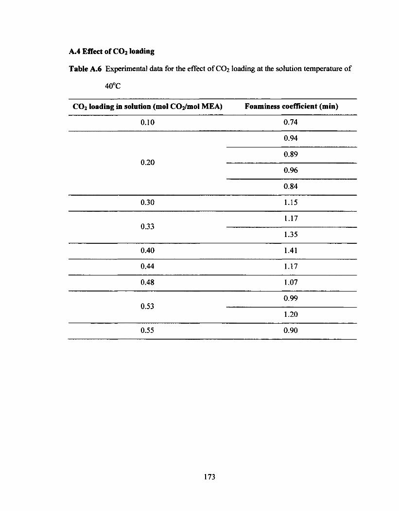
A.4 Effect of CO2 loading
Table A.6 Experimental data for the effect of CO2 loading at the solution temperature of
40°C
CO2 loading in solution (mol CO2/mol MEA) Foaminess coefficient (min)
0.10 0.74
0.94
0.89 0.20
0.96
0.84
0.30 1.15
1.17 0.33
1.35
0.40 1.41
0.44 1.17
0.48 1.07
0.99 0.53
1.20
0.55 0.90
173
A.4 Effect of CO2 loading
Table A.6 Experimental data for the effect of CO2 loading at the solution temperature of
40°C
C02 loading in solution (mol C02/mol MEA) Foansiness coefficient (min)
0.10 0.74
0.94
0.89 0.20
0.96
0.84
0.30 1.15
1.17 0.33
1.35
0.40 1.41
0.44 1.17
0.48 1.07
0.99 0.53
1.20
0.55 0.90
173

Table A.7 Experimental data for the effect of CO2 loading at the solution temperature of
60°C
CO2 loading in solution (mol CO2/mol MEA) Foaminess coefficient (min)
0.10 0.39
0.53
0.56
0.20 0.54
0.57
0.55
0.25 0.57
0.30 0.61
0.33 0.70
0.35 0.68
0.84
0.84
0.80 0.40
0.79
0.82
0.79
0.45 0.97
0.50 0.88
0.67 0.53
0.69
0.55 0.75
174
Table A.7 Experimental data for the effect of CO2 loading at the solution temperature of
60°C
CO2 loading In solution (mol C02/mol MEA) Foaminess coefficient (min)
0.10 0.39
0.53
0.56
0.20 0.54
0.57
0.55
0.25 0.57
0.30 0.61
0.33 0.70
0.35 0.68
0.84
0.84
0.80 0.40
0.79
0.82
0.79
0.45 0.97
0.50 0.88
0.67 0.53
0.69
0.55 0.75
174
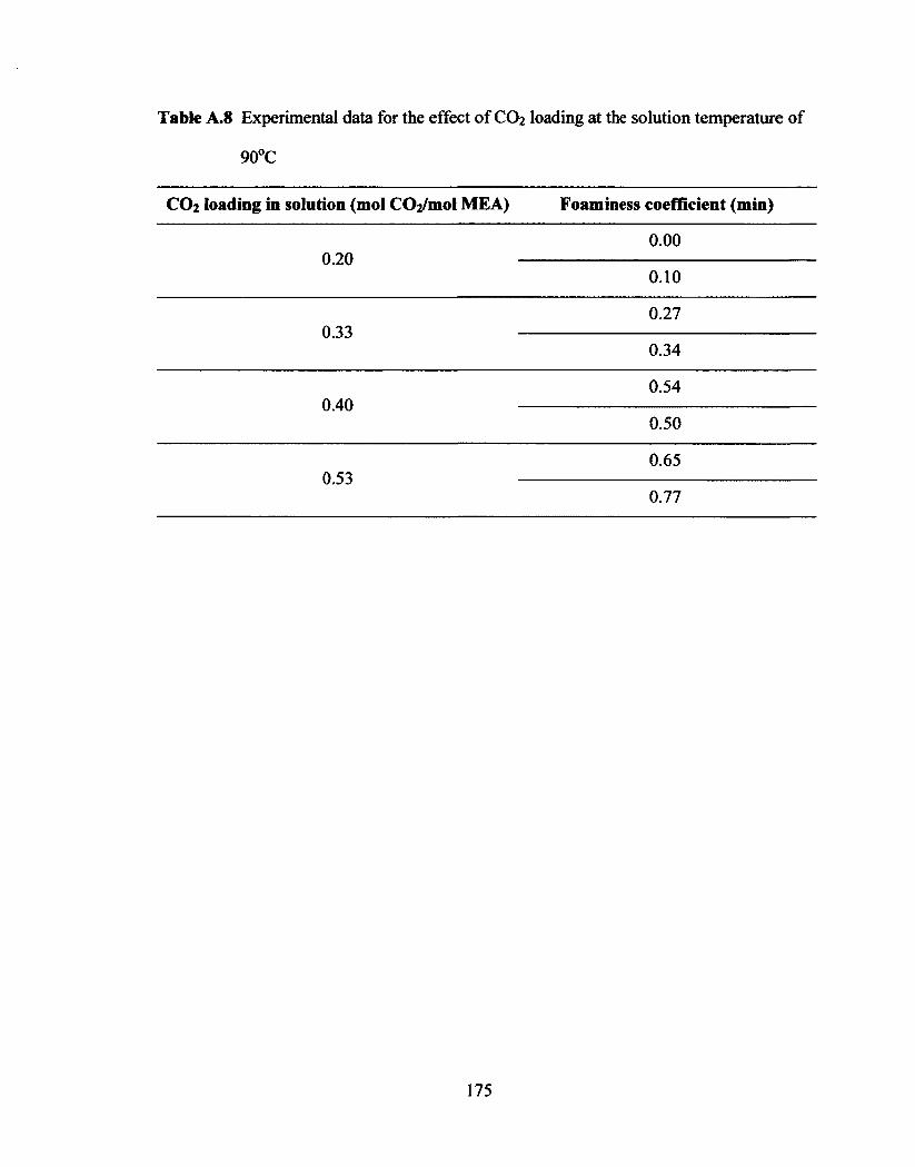
Table A.8 Experimental data for the effect of CO2 loading at the solution temperature of
90°C
CO2 loading in solution (mot CO2/mol MEA) Foaminess coefficient (min)
0.00 0.20
0.10
0.27 0.33
0.34
0.54 0.40
0.50
0.65 0.53
0.77
175
Table A.8 Experimental data for the effect of CO2 loading at the solution temperature of
90°C
CO2 loading in solution (mol CCVmol MEA) Foaminess coefficient (min)
0.00 0.20
0.10
0.27 0.33
0.34
0.54 0.40
0.50
0.65 0.53
0.77
175

A.5 Effect of solution temperature
Table A.9 Experimental data for the effect of solution temperature at the CO2 loading of
0.20 mol CO2/mol MEA
Solution temperature (°C) Foaminess coefficient (min)
0.84
40 0.94
0.89
0.73 50
0.72
0.56
0.54
60 0.53
0.57
0.55
0.27 70
0.30
0.02 80
0.22
0.00 90
0.10
176
A.5 Effect of solution temperature
Table A.9 Experimental data for the effect of solution temperature at the CO2 loading of
0.20 mol CCVmol MEA
Solution temperature (°C) Foaminess coefficient (min)
40
0.84
0.94
0.89
0.73 50
0.72
0.56
0.54
60 0.53
0.57
0.55
0.27 70
0.30
80 0.02
0.22
90 0.00
0.10
176

Table A.10 Experimental data for the effect of solution temperature at the CO2 loading
of 0.40 mol CO2/mol MEA
Solution temperature (°C) Foaminess coefficient (min)
40 1.41
1.02 50
0.94
0.79
0.82
0.79 60
0.80
0.84
0.84
0.68 70
0.65
0.54 80
0.58
0.54 90
0.50
177
Table A.10 Experimental data for the effect of solution temperature at the CO2 loading
of 0.40 mol CCVmol MEA
Solution temperature (°C) Foaminess coefficient (min)
40 1.41
1.02 50
0.94
0.79
0.82
0.79 60
0.80
0.84
0.84
0.68 70
0.65
0.54 80
0.58
90 0.54
0.50
177
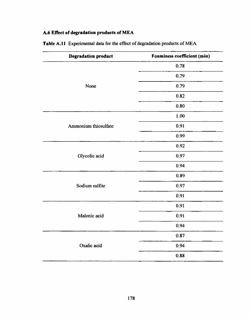
A.6 Effect of degradation products of MEA
Table A.11 Experimental data for the effect of degradation products of MEA
Degradation product Foaminess coefficient (min)
0.78
0.79
None 0.79
0.82
0.80
1.00
Ammonium thiosulfate 0.91
0.99
0.92
Glycolic acid 0.97
0.94
0.89
Sodium sulfite 0.97
0.91
0.91
Malonic acid 0.91
0.94
0.87
Oxalic acid 0.94
0.88
178
A.6 Effect of degradation products of MEA
Table A. 11 Experimental data for the effect of degradation products of MEA
Degradation product Foaminess coefficient (min)
0.78
0.79
None 0.79
0.82
0.80
1.00
Ammonium thiosulfate 0.91
0.99
0.92
Glycolic acid 0.97
0.94
0.89
Sodium sulfite 0.97
0.91
0.91
Malonic acid 0.91
0.94
0.87
Oxalic acid 0.94
0.88
178

Table A.11 Experimental data for the effect of degradation products of MEA (continued)
Degradation product Foaminess coefficient (min)
0.89
Sodium thiocyanate 0.92
0.89
0.90
Sodium chloride 0.89
0.89
0.83
Sodium thiosulfate 0.85
0.86
0.83
Bicine 0.86
0.85
0.80
Hydrochloric acid 0.87
0.82
0.85
Formic acid 0.79
0.84
0.86
Acetic acid 0.77
0.82
0.73
Sulfuric acid 0.78
0.80
179
Table A. 11 Experimental data for the effect of degradation products of ME A (continued)
Degradation product Foaminess coefficient (min)
0.89
Sodium thiocyanate 0.92
0.89
0.90
Sodium chloride 0.89
0.89
0.83
Sodium thiosulfate 0.85
0.86
0.83
Bicine 0.86
0.85
0.80
Hydrochloric acid 0.87
0.82
0.85
Formic acid 0.79
0.84
0.86
Acetic acid 0.77
0.82
0.73
Sulfuric acid 0.78
0.80
179

A.7 Effect of corrosion inhibitor
Table A.12 Experimental data for the effect of corrosion inhibitor
Corrosion inhibitor Foaminess coefficient (min)
0.78
0.79
None 0.79
0.82
0.80
0.99
Sodium metavanadate 1.00
1.05
0.88
Copper carbonate 0.96
0.97
0.83
Sodium sulfite 0.88
0.78
180
A. 7 Effect of corrosion inhibitor
Table A.12 Experimental data for the effect of corrosion inhibitor
Corrosion inhibitor Foaminess coefficient (min)
0.78
0.79
None 0.79
0.82
0.80
0.99
Sodium metavanadate 1.00
1.05
0.88
Copper carbonate 0.96
0.97
0.83
Sodium sulfite 0.88
0.78
180
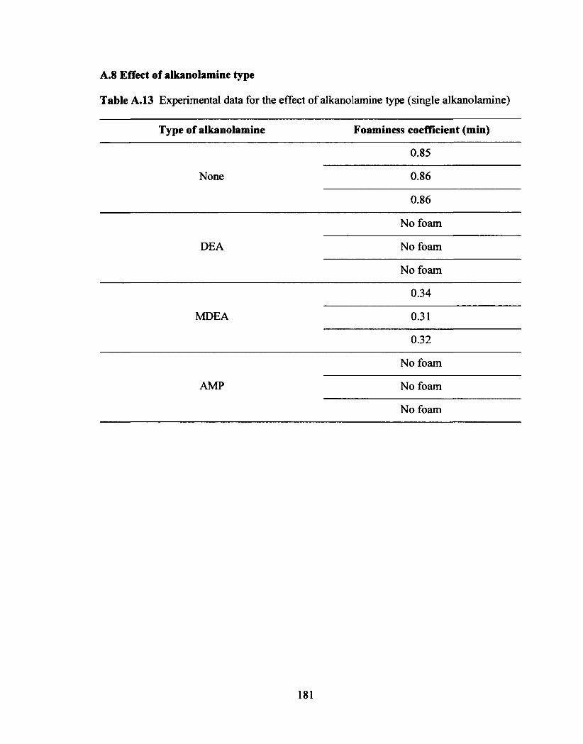
A.8 Effect of alkanolamine type
Table A.13 Experimental data for the effect of alkanolamine type (single alkanolamine)
Type of alkanolamine Foaminess coefficient (min)
0.85
None 0.86
0.86
No foam
DEA No foam
No foam
0.34
MDEA 0.31
0.32
No foam
AMP No foam
No foam
181
A.8 Effect of alkanolamine type
Table A. 13 Experimental data for the effect of alkanolamine type (single alkanolamine)
Type of alkanolamine Foaminess coefficient (min)
0.85
None 0.86
0.86
No foam
DEA No foam
No foam
MDEA
0.34
0.31
0.32
No foam
AMP No foam
No foam
181

Table A.14 Experimental data for the effect of alkanolamine type (blended
alkanolamine)
Type of alkanolamine Foaminess coefficient (min)
No foam
MEA + MDEA (1:2) No foam
No foam
No foam
MEA + MDEA (1:1) No foam
No foam
No foam
MEA + MDEA (2:1) No foam
No foam
No foam
DEA + MDEA (1:2) No foam
No foam
No foam
DEA + MDEA (1:1) No foam
No foam
No foam
DEA + MDEA (2:1) No foam
No foam
No foam
MEA + AMP (1:2) No foam
No foam
No foam
MEA + AMP (1:1) No foam
No foam
0.13
MEA + AMP (2:1) 0.13
0.13
182
Table A.14 Experimental data for the effect of alkanolamine type (blended
alkanolamine)
Type of alkanolamine Foaminess coefficient (min)
No foam
MEA + MDEA (1:2) No foam
No foam
No foam
MEA + MDEA (1:1) No foam
No foam
No foam
MEA + MDEA (2:1) No foam
No foam
No foam
DEA +MDEA (1:2) No foam
No foam
No foam
DEA + MDEA (1:1) No foam
No foam
No foam
DEA + MDEA (2:1) No foam
No foam
No foam
MEA + AMP (1:2) No foam
No foam
No foam
MEA + AMP (1:1) No foam
No foam
0.13
MEA + AMP (2:1) 0.13
0.13
182

Appendix B
Input parameters and simulation outputs of a foam height correlation
183
Appendix B
Input parameters and simulation outputs of a foam height correlation
183
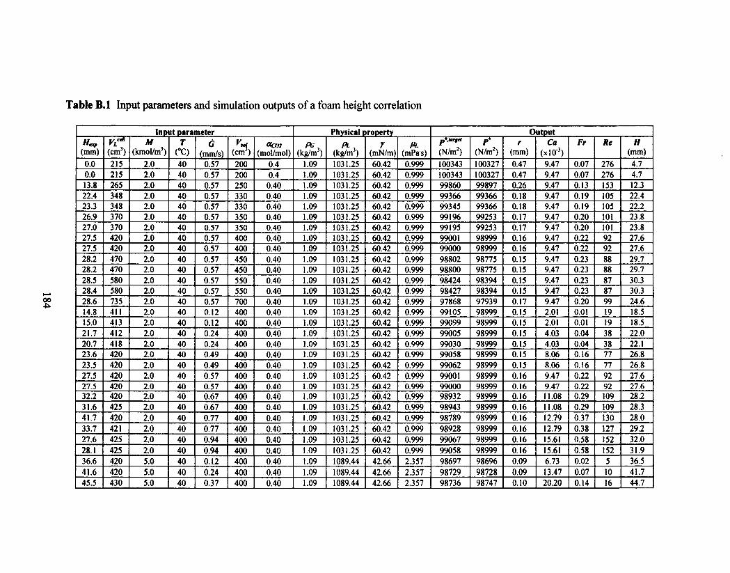
Table B.1 Input parameters and simulation outputs of a foam height correlation
Input parameter Physical property Output Heq,
(mm) Veen
(cm3) M
(kmolim3) T
(°C) 6
(mm/s) 11,1
(cm ) aco2
(mol/mol) p6
(kg/m3) ft
(kg/m3) y
(mN/m) IA
(mPa s) Pi "°'e" (N/m2)
P (N/m2)
r (mm)
Ca (x10-3)
Fr Re H (mm)
0.0 215 2.0 40 0.57 200 0.4 1.09 1031.25 60.42 0.999 100343 100327 0.47 9.47 0.07 276 4.7 0.0 215 2.0 40 0.57 200 0.4 1.09 1031.25 60.42 0.999 100343 100327 0.47 9.47 0.07 276 4.7 13.8 265 2.0 40 0.57 250 0.40 1.09 1031.25 60.42 0.999 99860 99897 0.26 9.47 0.13 153 12.3 22.4 348 2.0 40 0.57 330 0.40 1.09 1031.25 60.42 0.999 99366 99366 0.18 9.47 0.19 105 22.4 23.3 348 2.0 40 0.57 330 0.40 1.09 1031.25 60.42 0.999 99345 99366 0.18 9.47 0.19 105 22.2 26.9 370 2.0 40 0.57 350 0.40 1.09 1031.25 60.42 0.999 99196 99253 0.17 9.47 0.20 101 23.8 27.0 370 2.0 40 0.57 350 0.40 1.09 1031.25 60.42 0.999 99195 99253 0.17 9.47 0.20 101 23.8 27.5 420 2.0 40 0.57 400 0.40 1.09 1031.25 60.42 0.999 99001 98999 0.16 9.47 0.22 92 27.6 27.5 420 2.0 40 0.57 400 0.40 1.09 1031.25 60.42
._ 0.999 99000 98999 0.16 9.47 0.22 92 27.6
28.2 470 2.0 40 0.57 450 0.40 1.09 1031.25 60.42 0.999 98802 98775 0.15 9.47 0.23 88 29.7 28.2 470 2.0 40 0.57 450 0.40 1.09 1031.25 60.42 0.999 98800 98775 0.15 9.47 0.23 88 29.7 28.5 580 2.0 40 0.57 550 0.40 1.09 1031.25 60.42 0.999 98424 98394 0.15 9.47 0.23 87 30.3 28.4 580 2.0 40 0.57 550 0.40 1.09 1031.25 60.42 0.999 98427 98394 0.15 9.47 0.23 87 30.3 28.6 735 2.0 40 0.57 700 0.40 1.09 1031.25 60.42 0.999 97868 97939 0.17 9.47 0.20 99 24.6 14.8 411 2.0 40 0.12 400 0.40 1.09 1031.25 60.42 0.999 99105 98999 0.15 2.01 0.01 19 18.5 15.0 413 2.0 40 0.12 400 0.40 1.09 1031.25 60.42 0.999 99099 98999 0.15 2.01 0.01 19 18.5 21.7 412 2.0 40 0.24 400 0.40 1.09 1031.25 60.42 0.999 99005 98999 0.15 4.03 0.04 38 22.0 20.7 418 2.0 40 0.24 400 0.40 1.09 1031.25 60.42 0.999 99030 98999 0.15 4.03 0.04 38 22.1 23.6 420 2.0 40 0.49 400 0.40 1.09 1031.25 60.42 0.999 99058 98999 0.15 8.06 0.16 77 26.8 23.5 420 2.0 40 0.49 400 0.40 1.09 1031.25 60.42 0.999 99062 98999 0.15 8.06 0.16 77 26.8 27.5 420 2.0 40 0.57 400 0.40 1.09 1031.25 60.42 0.999 99001 98999 0.16 9.47 0.22 92 27.6 27.5 420 2.0 40 0.57 400 0.40 1.09 1031.25 60.42 0.999 99000 98999 0.16 9.47 0.22 92 27.6 32.2 420 2.0 40 0.67 400 0.40 1.09 1031.25 60.42 0.999 98932 98999 0.16 11.08 0.29 109 28.2 31.6 425 2.0 40 0.67 400 0.40 1.09 1031.25 60.42 0.999 98943 98999 0.16 11.08 0.29 109 28.3 41.7 420 2.0 40 0.77 400 0.40 1.09 1031.25 60.42 0.999 98789 98999 0.16 12.79 0.37 130 28.0 33.7 421 2.0 40 0.77 400 0.40 1.09 1031.25 60.42 0.999 98928 98999 0.16 12.79 0.38 127 29.2 27.6 425 2.0 40 0.94 400 0.40 1.09 1031.25 60.42 0.999 99067 98999 0.16 15.61 0.58 152 32.0 28.1 425 2.0 40 0.94 400 0.40 1.09 1031.25 60.42 0.999 99058 98999 0.16 15.61 0.58 152 31.9 36.6 420 5.0 40 0.12 400 0.40 1.09 1089.44 42.66 2.357 98697 98696 0.09 6.73 0.02 5 36.5 41.6 420 5.0 40 0.24 400 0.40 1.09 1089.44 42.66 2.357 98729 98728 0.09 13.47 0.07 10 41.7 45.5 430 5.0 40 0.37 400 0.40 1.09 1089.44 42.66 2.357 98736 98747 0.10 20.20 0.14 16 44.7
Table B.1 Input parameters and simulation outputs of a foam height correlation
00
Input parameter Physical property Output
(mm) yL"*
(cm3) M
(kmol/m3) r
CC) G
(mm/s) K"! (cm3)
OC02 (mol/mol)
PC, (kg/m3) (kg/m3)
7 (mN/m)
At (mPas)
p*,Urttt
(N/m2) P*
(N/m2) r
(mm) Ca
(xl0°) Fr Re H
(mm)
0.0 215 2.0 40 0.57 200 0.4 1.09 1031.25 60.42 0.999 100343 100327 0.47 9.47 0.07 276 4.7 0.0 215 2.0 40 0.57 200 0.4 1.09 1031.25 60.42 0.999 100343 100327 0.47 9.47 0.07 276 4.7 13.8 265 2.0 40 0.57 250 0.40 1.09 1031.25 60.42 0.999 99860 99897 0.26 9.47 0.13 153 12.3 22.4 348 2.0 40 0.57 330 0.40 1.09 1031.25 60.42 0.999 99366 99366 0.18 9.47 0.19 105 22.4 23.3 348 2.0 40 0.57 330 0.40 1.09 1031.25 60.42 0.999 99345 99366 0.18 9.47 0.19 105 22.2 26.9 370 2.0 40 0.57 350 0.40 1.09 1031.25 60.42 0.999 991% 99253 0.17 9.47 0.20 101 23.8 27.0 370 2.0 40 0.57 350 0.40 1.09 1031.25 60.42 0.999 99195 99253 0.17 9.47 0.20 101 23.8 27.5 420 2.0 40 0.57 400 0.40 1.09 1031.25 60.42 0.999 99001 98999 0.16 9.47 0.22 92 27.6 27.5 420 2.0 40 0.57 400 0.40 1.09 1031.25 60.42 0.999 99000 98999 0.16 9.47 0.22 92 27.6 28.2 470 2.0 40 0.57 450 0.40 1.09 1031.25 60.42 0.999 98802 98775 0.15 9.47 0.23 88 29.7 28.2 470 2.0 40 0.57 450 0.40 1.09 1031.25 60.42 0.999 98800 98775 0.15 9.47 0.23 88 29.7 28.5 580 2.0 40 0.57 550 0.40 1.09 1031.25 60.42 0.999 98424 98394 0.15 9.47 0.23 87 30.3 28.4 580 2.0 40 0.57 550 0.40 1.09 1031.25 60.42 0.999 98427 98394 0.15 9.47 0.23 87 30.3 28.6 735 2.0 40 0.57 700 0.40 1.09 1031.25 60.42 0.999 97868 97939 0.17 9.47 0.20 99 24.6 14.8 411 2.0 40 0.12 400 0.40 1.09 1031.25 60.42 0.999 99105 98999 0.15 2.01 0.01 19 18.5 15.0 413 2.0 40 0.12 400 0.40 1.09 1031.25 60.42 0.999 99099 98999 0.15 2.01 0.01 19 18.5 21.7 412 2.0 40 0.24 400 0.40 1.09 1031.25 60.42 0.999 99005 98999 0.15 4.03 0.04 38 22.0 20.7 418 2.0 40 0.24 400 0.40 1.09 1031.25 60.42 0.999 99030 98999 0.15 4.03 0.04 38 22.1 23.6 420 2.0 40 0.49 400 0.40 1.09 1031.25 60.42 0.999 99058 98999 0.15 8.06 0.16 77 26.8 23.5 420 2.0 40 0.49 400 0.40 1.09 1031.25 60.42 0.999 99062 98999 0.15 8.06 0.16 77 26.8 27.5 420 2.0 40 0.57 400 0.40 1.09 1031.25 60.42 0.999 99001 98999 0.16 9.47 0.22 92 27.6 27.5 420 2.0 40 0.57 400 0.40 1.09 1031.25 60.42 0.999 99000 98999 0.16 9.47 0.22 92 27.6 32.2 420 2.0 40 0.67 400 0.40 1.09 1031.25 60.42 0.999 98932 98999 0.16 11.08 0.29 109 28.2 31.6 425 2.0 40 0.67 400 0.40 1.09 1031.25 60.42 0.999 98943 98999 0.16 11.08 0.29 109 28.3 41.7 420 2.0 40 0.77 400 0.40 1.09 1031.25 60.42 0.999 98789 98999 0.16 12.79 0.37 130 28.0 33.7 421 2.0 40 0.77 400 0.40 1.09 1031.25 60.42 0.999 98928 98999 0.16 12.79 0.38 127 29.2 27.6 425 2.0 40 0.94 400 0.40 1.09 1031.25 60.42 0.999 99067 98999 0.16 15.61 0.58 152 32.0 28.1 425 2.0 40 0.94 400 0.40 1.09 1031.25 60.42 0.999 99058 98999 0.16 15.61 0.58 152 31.9 36.6 420 5.0 40 0.12 400 0.40 1.09 1089.44 42.66 2.357 98697 98696 0.09 6.73 0.02 5 36.5 41.6 420 5.0 40 0.24 400 0.40 1.09 1089.44 42.66 2.357 98729 98728 0.09 13.47 0.07 10 41.7 45.5 430 5.0 40 0.37 400 0.40 1.09 1089.44 42.66 2.357 98736 98747 0.10 20.20 0.14 16 44.7

Table B.1 Input parameters and simulation outputs of a foam height correlation (continued)
Input parameter Physical property Output H.?
(mm) VL" R(cm3)
M (kmol/m3)
T (°C)
G (mm/s)
Vsof (cm )
aCO2 (mol/mol)
PG , (kg/m')
Pi (kg/m3)
r(mN/m)
pi,(mPa s)
?And
(N/m2)
10
(N/m2)
r
(mm)
Ca
(x10-3)
Fr Re H(mm)
47.0 425 5.0 40 0.43 400 0.40 1.09 1089.44 42.66 2.357 98740 98754 0.10 23.57 0.19 19 45.9 48.3 425 5.0 40 0.49 400 0.40 1.09 1089.44 42.66 2.357 98744 98760 0.10 26.94 0.25 22 46.9 48.4 425 5.0 40 0.57 400 0.40 1.09 1089.44 42.66 2.357 98769 98767 0.10 31.65 0.34 26 48.5 59.4 420 5.0 40 0.61 400 0.40 1.09 1089.44 42.66 2.357 98632 98770 0.10 33.67 0.37 29 46.5 55.5 420 5.0 40 0.67 400 0.40 1.09 1089.44 42.66 2.357 98700 98774 0.10 37.04 0.45 31 48.5 47.5 425 5.0 40 0.77 400 0.40 1.09 1089.44 42.66 2.357 98828 98781 0.10 42.77 0.61 36 52.0 52.3 425 5.0 40 0.94 400 0.40 1.09 1089.44 42.66 2.357 98796 98790 0.10 52.20 0.89 45 52.9 21.1 412 2.0 60 0.57 400 0.40 1.02 1020.90 58.76 0.693 99116 99121 0.17 6.75 0.20 144 20.8 21.6 425 2.0 60 0.57 400 0.40 1.02 1020.90 58.76 0.693 99106 99121 0.17 6.75 0.19 145 20.8 21.6 428 2.0 60 0.57 400 0.40 1.02 1020.90 58.76 0.693 99105 99121 0.17 6.75 0.19 145 20.8 22.3 425 3.0 60 0.57 400 0.40 1.02 1039.72 53.14 0.879 99108 99061 0.15 9.48 0.23 101 24.8 24.7 425 3.0 60 0.57 400 0.40 1.02 1039.72 53.14 0.879 99058 99061 0.15 9.48 0.22 101 24.5 24.9 428 3.0 60 0.57 400 0.40 1.02 1039.72 53.14 0.879 99054 99061 0.15 9.48 0.22 101 24.5 29.2 425 4.0 60 0.57 400 0.40 1.02 1058.46 47.21 1.147 98999 98998 0.13 13.91 0.26 68 29.3 29.5 423 4.0 60 0.57 400 0.40 1.02 1058.46 47.21 1.147 98995 98998 0.13 13.91 0.26 68 29.2 29.4 420 4.0 60 0.57 400 0.40 1.02 1058.46 47.21 1.147 98995 98998 0.13 13.91 0.26 68 29.2 27.1 430 5.0 60 0.57 400 0.40 1.02 1077.12 40.97 1.540 99072 99041 0.12 21.53 0.27 49 29.3 27.2 430 5.0 60 0.57 400 0.40 1.02 1077.12 40.97 1.540 99071 99041 0.12 21.53 0.27 49 29.3 28.1 430 5.0 60 0.57 400 0.40 1.02 1077.12 40.97 1.540 99055 99041 0.12 21.53 0.27 49 29.1 28,7 425 5.0 60 0.57 400 0.40 1.02 1077.12 40.97 1.540 99045 99041 0.12 21.53 0.27 49 29.0 28.9 430 5.0 60 0.57 400 0.40 1.02 1077.12 40.97 1.540 99041 99041 0.12 21.53 0.27 50 29.0 31.9 428 6.0 60 0.57 400 0.40 1.02 1095.64 34.42 2.131 99038 99139 0.13 35.46 0.26 38 24.2 30.2 430 6.0 60 0.57 400 0.40 1.02 1095.64 34.42 2.131 99064 99139 0.13 35.46 0.26 38 24.5 26.9 432 6.0 60 0.57 400 0.40 1.02 1095.64 34.42 2.131 99115 99139 0.13 35.46 0.26 37 25.2 24.8 428 7.0 60 0.57 400 0.40 1.02 1114.01 27.55 3.041 99191 99193 0.12 63.22 0.28 25 24.6 25.3 430 7.0 60 0.57 400 0.40 1.02 1114.01 27.55 3.041 99183 99193 0.12 63.22 0.28 25 24.5 24.4 430 7.0 60 0.57 400 0.40 1.02 1114.01 27.55 3.041 991% 99193 0.12 63.22 0.28 25 24.7 27.9 420 2.0 40 0.57 400 0.20 1.09 1013.96 61.81 0.950 99015 99019 0.16 8.80 0.21 97 27.6 26.0 420 2.0 40 0.57 400 0.20 1.09 1013.96 61.81 0.950 99054 99019 0.16 8.80 0.21 96 27.9 27.4 420 2.0 40 0.57 400 0.20 1.09 1013.96 61.81 0.950 99026 99019 0.16 8.80 0.21 96 27.7 33.1 422 3.0 40 0.57 400 0.20 1.09 1024.75 58.78 1.184 98941 98959 0.14 11.54 0.23 72 31.9
Table B.l Input parameters and simulation outputs of a foam height correlation (continued)
Input parameter Physical property Output
(mm) VL (cm3)
M (kmol/m3)
T (°C)
G (mm/s)
V«4 (ct$)
Ocoi (mol/mol)
A,' (kg/m3)
A3 (kg/m3) r
(mN/m) fk.
(mPas)
p",target (N/m2)
/>'
(N/m2) r
(mm) Ca
(xl0}) FT Re H
(mm)
47.0 425 5.0 40 0.43 400 0.40 1.09 1089.44 42.66 2.357 98740 98754 0.10 23.57 0.19 19 45.9 48.3 425 5.0 40 0.49 400 0.40 1.09 1089.44 42.66 2.357 98744 98760 0.10 26.94 0.25 22 46.9 48.4 425 5.0 40 0.57 400 0.40 1.09 1089.44 42.66 2.357 98769 98767 0.10 31.65 0.34 26 48.5 59.4 420 5.0 40 0.61 400 0.40 1.09 1089.44 42.66 2.357 98632 98770 0.10 33.67 0.37 29 46.5 55.5 420 5.0 40 0.67 400 0.40 1.09 1089.44 42.66 2.357 98700 98774 0.10 37.04 0.45 31 48.5 47.5 425 5.0 40 0.77 400 0.40 1.09 1089.44 42.66 2.357 98828 98781 0.10 42.77 0.61 36 52.0 52.3 425 5.0 40 0.94 400 0.40 1.09 1089.44 42.66 2.357 987% 98790 0.10 52.20 0.89 45 52.9 21.1 412 2.0 60 0.57 400 0.40 1.02 1020.90 58.76 0.693 99116 99121 0.17 6.75 0.20 144 20.8 21.6 425 2.0 60 0.57 400 0.40 1.02 1020.90 58.76 0.693 99106 99121 0.17 6.75 0.19 145 20.8 21.6 428 2.0 60 0.57 400 0.40 1.02 1020.90 58.76 0.693 99105 99121 0.17 6.75 0.19 145 20.8 22.3 425 3.0 60 0.57 400 0.40 1.02 1039.72 53.14 0.879 99108 99061 0.15 9.48 0.23 101 24.8 24.7 425 3.0 60 0.57 400 0.40 1.02 1039.72 53.14 0.879 99058 99061 0.15 9.48 0.22 101 24.5 24.9 428 3.0 60 0.57 400 0.40 1.02 1039.72 53.14 0.879 99054 99061 0.15 9.48 0.22 101 24.5 29.2 425 4.0 60 0.57 400 0.40 1.02 1058.46 47.21 1.147 98999 98998 0.13 13.91 0.26 68 29.3 29.5 423 4.0 60 0.57 400 0.40 1.02 1058.46 47.21 1.147 98995 98998 0.13 13.91 0.26 68 29.2 29.4 420 4.0 60 0.57 400 0.40 1.02 1058.46 47.21 1.147 98995 98998 0.13 13.91 0.26 68 29.2 27.1 430 5.0 60 0.57 400 0.40 1.02 1077.12 40.97 1.540 99072 99041 0.12 21.53 0.27 49 29.3 27.2 430 5.0 60 0.57 400 0.40 1.02 1077.12 40.97 1.540 99071 99041 0.12 21.53 0.27 49 29.3 28.1 430 5.0 60 0.57 400 0.40 1.02 1077.12 40.97 1.540 99055 99041 0.12 21.53 0.27 49 29.1 28.7 425 5.0 60 0.57 400 0.40 1.02 1077.12 40.97 1.540 99045 99041 0.12 21.53 0.27 49 29.0 28.9 430 5.0 60 0.57 400 0.40 1.02 1077.12 40.97 1.540 99041 99041 0.12 21.53 0.27 50 29.0 31.9 428 6.0 60 0.57 400 0.40 1.02 1095.64 34.42 2.131 99038 99139 0.13 35.46 0.26 38 24.2 30.2 430 6.0 60 0.57 400 0.40 1.02 1095.64 34.42 2.131 99064 99139 0.13 35.46 0.26 38 24.5 26.9 432 6.0 60 0.57 400 0.40 1.02 1095.64 34.42 2.131 99115 99139 0.13 35.46 0.26 37 25.2 24.8 428 7.0 60 0.57 400 0.40 1.02 1114.01 27.55 3.041 99191 99193 0.12 63.22 0.28 25 24.6 25.3 430 7.0 60 0.57 400 0.40 1.02 1114.01 27.55 3.041 99183 99193 0.12 63.22 0.28 25 24.5 24.4 430 7.0 60 0.57 400 0.40 1.02 1114.01 27.55 3.041 991% 99193 0.12 63.22 0.28 25 24.7 27.9 420 2.0 40 0.57 400 0.20 1.09 1013.96 61.81 0.950 99015 99019 0.16 8.80 0.21 97 27.6 26.0 420 2.0 40 0.57 400 0.20 1.09 1013.96 61.81 0.950 99054 99019 0.16 8.80 0.21 % 27.9 27.4 420 2.0 40 0.57 400 0.20 1.09 1013.96 61.81 0.950 99026 99019 0.16 8.80 0.21 % 27.7 33.1 422 3.0 40 0.57 400 0.20 1.09 1024.75 58.78 1.184 98941 98959 0.14 11.54 0.23 72 31.9

Table B.1 Input parameters and simulation outputs of a foam height correlation (continued)
Input parameter Physical property Output Hem,
(mm) Well(cm3)
M (kmol/m3)
T (°C)
G (mm/s)
vul(cm )
aCO2 (mol/mol)
Pc (kg/m3)
Pt. (kg/m3)
y (mN/m)
Pt (mPa s)
P* ""r" (N/m2)
P*(N/m2)
r (mm)
Ca (x10)
Fr Re H (mm)
32.3 422 3.0 40 0.57 400 0.20 1.09 1024.75 58.78 1.184 98956 98959 0.14 11.54 0.23 71 32.1 32.9 425 3.0 40 0.57 400 0.20 1.09 1024.75 58.78 1.184 98944 98959 0.14 11.54 0.23 72 32.0 33.0 428 5.0 40 0.57 400 0.20 1.09 1046.09 52.09 1.973 99007 99016 0.14 21.70 0.23 44 32.4 32.4 425 5.0 40 0.57 400 0.20 1.09 1046.09 52.09 1.973 99017 99016 0.14 21.70 0.23 44 32.5 30.6 425 5.0 40 0.57 400 0.20 1.09 1046.09 52.09 1.973 99047 99016 0.14 21.70 0.23 43 32.8 33.0 425 5.5 40 0.57 400 0.20 1.09 1051.36 50.27 2.276 99024 99034 0.14 25.93 0.23 38 32.3 31.9 425 5.5 40 0.57 400 0.20 1.09 1051.36 50.27 2.276 99043 99034 0.14 25.93 0.23 38 . 32.5 33.3 428 5.5 40 0.57 400 0.20 1.09 1051.36 50.27 2.276 99019 99034 0.14 25.93 0.23 38 32.2 30.7 425 6.0 40 0.57 400 0.20 1.09 1056.60 48.40 2.641 99079 99107 0.16 31.26 0.21 36 28.6 27.9 425 6.0 40 0.57 400 0.20 1.09 1056.60 48.40 2.641 99124 99107 0.15 31.26 0.22 35 29.1 32.8 428 6.0 40 0.57 400 0.20 1.09 1056.60 48.40 2.641 99045 99107 0.16 31.26 0.21 36 28.2 24.5 435 7.0 40 0.57 400 0.20 1.09 1066.96 44.47 3.624 99210 99161 0.16 46.68 0.21 26 28.3 24.1 430 7.0 40 0.57 400 0.20 1.09 1066.96 44.47 3.624 99216 99161 0.16 46.68 0.21 26 28.4 24.4 430 7.0 40 0.57 400 0.20 1.09 1066.96 44.47 3.624 99212 99161 0.16 46.68 0.21 26 28.3 25.4 423 5.0 40 0.57 400 0.10 1.09 1024.41 56.95 1.805 99148 99265 0.22 18.16 0.15 70 18.5 29.0 425 5.0 40 0.57 400 0.20 1.09 1046.09 52.09 1.973 99075 99016 0.14 21.70 0.24 43 33.1 33.0 428 5.0 40 0.57 400 0.20 1.09 1046.09 52.09 1.973 99007 99016 0.14 21.70 0.23 44 32.4 39.4 428 5.0 40 0.57 400 0.30 1.09 1067.76 47.32 2.157 98899 98870 0.12 26.11 0.29 33 41.8 40.1 429 5.0 40 0.57 400 0.33 1.09 1074.27 45.92 2.215 98889 98836 0.11 27.63 0.31 30 44.4 46.4 429 5.0 40 0.57 400 0.33 1.09 1074.27 45.92 2.215 98796 98836 0.11 27.63 0.30 31 43.0 40.4 420 5.0 40 0.57 400 0.44 1.09 1098.10 40.82 2.443 98882 98965 0.12 34.28 0.28 31 33.6 36.9 423 5.0 40 0.57 400 0.48 1.09 1106.77 39.00 2.531 98933 98956 0.11 37.18 0.29 29 34.9 34.1 425 5.0 40 0.57 400 0.53 1.09 1117.60 36.74 2.647 98972 98947 0.11 41.26 0.31 26 36.3 41.2 425 5.0 40 0.57 400 0.53 1.09 1117.60 36.74 2.647 98871 98947 0.11 41.26 0.30 27 34.6 31.1 420 5.0 40 0.57 400 0.55 1.09 1121.94 35.84 2.694 99017 98943 0.10 43.06 0.32 25 37.3 13.6 428 5.0 60 0.57 400 0.10 1.02 1012.83 54.13 1.162 99382 99540 0.36 12.30 0.09 181 6.8 19.5 430 5.0 60 0.57 400 0.20 1.02 1034.26 49.66 1.276 99236 99290 0.20 14.72 0.17 92 16.5 18.9 430 5.0 60 0.57 400 0.20 1.02 1034.26 49.66 1.276 99248 99290 0.20 14.72 0.17 92 16.6 19.1 428 5.0 60 0.57 400 0.20 1.02 1034.26 49.66 1.276 99243 99290 0.20 14.72 0.17 92 16.6 18.7 430 5.0 60 0.57 400 0.20 1.02 1034.26 49.66 1.276 99252 99290 0.20 14.72 0.17 91 16.6 18.4 428 5.0 60 0.57 400 0.20 1.02 1034.26 49.66 1.276 99258 99290 0.20 14.72 0.17 91 16.7
Table B.1 Input parameters and simulation outputs of a foam height correlation (continued)
00 On
Input parameter Physical property Output
(mm) VL (cm3)
M (kmol/m3)
T (°C)
6 (mm/s) (cm3)
OC02 (mol/mol)
A. , (kg/m ) (kg/m )
r (mN/m)
tk. (mPas)
p'.arfrt
(N/m2) Pl
(N/m2) T
(mm) Ca
(xlO"3) Fr Re H
(mm)
32.3 422 3.0 40 0.57 400 0.20 1.09 1024.75 58.78 1.184 98956 98959 0.14 11.54 0.23 71 32.1 32.9 425 3.0 40 0.57 400 0.20 1.09 1024.75 58.78 1.184 98944 98959 0.14 11.54 0.23 72 32.0 33.0 428 5.0 40 0.57 400 0.20 1.09 1046.09 52.09 1.973 99007 99016 0.14 21.70 0.23 44 32.4 32.4 425 5.0 40 0.57 400 0.20 1.09 1046.09 52.09 1.973 99017 99016 0.14 21.70 0.23 44 32.5 30.6 425 5.0 40 0.57 400 0.20 1.09 1046.09 52.09 1.973 99047 99016 0.14 21.70 0.23 43 32.8 33.0 425 5.5 40 0.57 400 0.20 1.09 1051.36 50.27 2.276 99024 99034 0.14 25.93 0.23 38 32.3 31.9 425 5.5 40 0.57 400 0.20 1.09 1051.36 50.27 2.276 99043 99034 0.14 25.93 0.23 38 . 32.5 33.3 428 5.5 40 0.57 400 0.20 1.09 1051.36 50.27 2.276 99019 99034 0.14 25.93 0.23 38 32.2 30.7 425 6.0 40 0.57 400 0.20 1.09 1056.60 48.40 2.641 99079 99107 0.16 31.26 0.21 36 28.6 27.9 425 6.0 40 0.57 400 0.20 1.09 1056.60 48.40 2.641 99124 99107 0.15 31.26 0.22 35 29.1 32.8 428 6.0 40 0.57 400 0.20 1.09 1056.60 48.40 2.641 99045 99107 0.16 31.26 0.21 36 28.2 24.5 435 7.0 40 0.57 400 0.20 1.09 1066.% 44.47 3.624 99210 99161 0.16 46.68 0.21 26 28.3 24.1 430 7.0 40 0.57 400 0.20 1.09 1066.96 44.47 3.624 99216 99161 0.16 46.68 0.21 26 28.4 24.4 430 7.0 40 0.57 400 0.20 1.09 1066.96 44.47 3.624 99212 99161 0.16 46.68 0.21 26 28.3 25.4 423 5.0 40 0.57 400 0.10 1.09 1024.41 56.95 1.805 99148 99265 0.22 18.16 0.15 70 18.5 29.0 425 5.0 40 0.57 400 0.20 1.09 1046.09 52.09 1.973 99075 99016 0.14 21.70 0.24 43 33.1 33.0 428 5.0 40 0.57 400 0.20 1.09 1046.09 52.09 1.973 99007 99016 0.14 21.70 0.23 44 32.4 39.4 428 5.0 40 0.57 400 0.30 1.09 1067.76 47.32 2.157 98899 98870 0.12 26.11 0.29 33 41.8 40.1 429 5.0 40 0.57 400 0.33 1.09 1074.27 45.92 2.215 98889 98836 0.11 27.63 0.31 30 44.4 46.4 429 5.0 40 0.57 400 0.33 1.09 1074.27 45.92 2.215 98796 98836 0.11 27.63 0.30 31 43.0 40.4 420 5.0 40 0.57 400 0.44 1.09 1098.10 40.82 2.443 98882 98965 0.12 34.28 0.28 31 33.6 36.9 423 5.0 40 0.57 400 0.48 1.09 1106.77 39.00 2.531 98933 98956 0.11 37.18 0.29 29 34.9 34.1 425 5.0 40 0.57 400 0.53 1.09 1117.60 36.74 2.647 98972 98947 0.11 41.26 0.31 26 36.3 41.2 425 5.0 40 0.57 400 0.53 1.09 1117.60 36.74 2.647 98871 98947 0.11 41.26 0.30 27 34.6 31.1 420 5.0 40 0.57 400 0.55 1.09 1121.94 35.84 2.694 99017 98943 0.10 43.06 0.32 25 37.3 13.6 428 5.0 60 0.57 400 0.10 1.02 1012.83 54.13 1.162 99382 99540 0.36 12.30 0.09 181 6.8 19.5 430 5.0 60 0.57 400 0.20 1.02 1034.26 49.66 1.276 99236 99290 0.20 14.72 0.17 92 16.5 18.9 430 5.0 60 0.57 400 0.20 1.02 1034.26 49.66 1.276 99248 99290 0.20 14.72 0.17 92 16.6 19.1 428 5.0 60 0.57 400 0.20 1.02 1034.26 49.66 1.276 99243 99290 0.20 14.72 0.17 92 16.6 18.7 430 5.0 60 0.57 400 0.20 1.02 1034.26 49.66 1.276 99252 99290 0.20 14.72 0.17 91 16.6 18.4 428 5.0 60 0.57 400 0.20 1.02 1034.26 49.66 1.276 99258 99290 0.20 14.72 0.17 91 16.7

Table B.1 Input parameters and simulation outputs of a foam height correlation (continued)
Input parameter Physical . roperty Output Hen,
(mm) VLC (cm3)
M (kmol/m3)
T (°C)
G (mm/s)
V1(cm )
(km (mol/mol)
Ac (kg/m3)
Pi. (kg/m3)
7 (mN/m)
iit
(mPa s)
parr*
(N/m2)
,..
(N/m2) r
(mm) Ca
(x 1 0) Fr Re H
(mm)
19.6 428 5.0 60 0.57 400 0.25 1.02 1044.97 47.45 1.338 99226 99210 0.17 16.15 0.20 75 20.6 21.0 428 5.0 60 0.57 400 0.30 1.02 1055.69 45.27 1.402 99193 99144 0.15 17.74 0.23 64 24.0 24.0 430 5.0 60 0.57 400 0.33 1.02 1062.12 43.97 1.442 99134 99110 0.14 18.78 0.24 59 25.5 23.5 428 5.0 60 0.57 400 0.35 1.02 1066.40 43.11 1.469 99141 99089 0.13 19.52 0.25 56 26.9 27.4 430 5.0 60 0.57 400 0.40 1.02 1077.12 40.97 1.540 99068 99041 0.12 21.53 0.27 49 29.2 27.2 430 5.0 60 0.57 400 0.40 1.02 1077.12 40.97 1.540 99071 99041 0.12 21.53 0.27 49 29.3 28.1 430 5.0 60 0.57 400 0.40 1.02 1077.12 40.97 1.540 99055 99041 0.12 21.53 0.27 49 29.1 33.3 428 5.0 60 0.57 400 0.45 1.02 1087.83 38.85 1.614 98968 98999 0.11 23.79 0.29 44 31.0 30.2 428 5.0 60 0.57 400 0.50 1.02 1098.54 36.75 1.691 99016 98961 0.10 26.36 0.32 39 34.4 23.0 427 5.0 60 0.57 400 0.53 1.02 1104.97 35.50 1.740 99136 99047 0.11 28.07 0.30 41 29.3 23.6 425 5.0 60 0.57 400 0.53 1.02 1104.97 35.50 1.740 99124 99047 0.11 28.07 0.30 41 29.1 25.9 425 5.0 60 0.57 400 0.55 1.02 1109.25 34.67 1.772 99085 99043 0.11 29.28 0.30 40 28.9 0.0 440 5.0 90 0.57 400 0.20 0.94 1012.98 46.11 0.763 99684 99565 0.30 9.48 0.11 229 6.9 3.3 440 5.0 90 0.57 400 0.20 0.94 1012.98 46.11 0.763 99635 99565 0.31 9.48 0.11 235 6.6 9.3 439 5.0 90 0.57 400 0.33 0.94 1040.27 41.20 0.867 99457 99385 0.19 12.05 0.17 133 12.5 11.5 436 5.0 90 0.57 400 0.33 0.94 1040.27 41.20 0.867 99399 99385 0.20 12.05 0.17 135 12.2 18.5 440 5.0 90 0.57 400 0.40 0.94 1054.96 38.61 0.928 99235 99315 0.17 13.77 0.19 112 14.2 17.3 440 5.0 90 0.57 400 0.40 0.94 1054.96 38.61 0.928 99259 99315 0.17 13.77 0.20 111 14.3 22.4 450 5.0 90 0.57 400 0.53 0.94 1082.25 33.86 1.055 99147 99214 0.14 17.84 0.25 80 18.3 26.3 440 5.0 90 0.57 400 0.53 0.94 1082.25 33.86 1.055 99077 99214 0.14 17.84 0.24 81 17.7 29.0 425 5.0 40 0.57 400 0.20 1.09 1046.09 52.09 1.973 99075 99016 0.14 21.70 0.24 43 33.1 26.4 425 5.0 40 0.57 400 0.20 1.09 1046.09 52.09 1.973 99118 99016 0.14 21.70 0.24 43 33.6 25.1 425 5.0 50 0.57 400 0.20 1.06 1040.44 50.87 1.569 99133 99167 0.17 17.67 0.20 64 23.0 24.6 429 5.0 50 0.57 400 0.20 1.06 1040.44 50.87 1.569 99141 99167 0.17 17.67 0.20 64 23.0 19.1 428 5.0 60 0.57 400 0.20 1.02 1034.26 49.66 1.276 99243 99290 0.20 14.72 0.17 92 16.6 18.7 430 5.0 60 0.57 400 0.20 1.02 1034.26 49.66 1.276 99252 99290 0.20 14.72 0.17 91 16.6 9.4 430 5.0 70 0.57 400 0.2 0.99 1027.60 48.46 1.060 99467 99395 0.22 12.53 0.15 124 12.6 10.4 435 5.0 70 0.57 400 0.2 0.99 1027.60 48.46 1.060 99439 99395 0.23 12.53 0.15 125 12.5 0.8 435 5.0 80 0.57 400 0.2 0.97 1020.50 47.28 0.894 99670 99485 0.25 10.84 0.13 165 9.7 7.6 435 5.0 80 0.57 400 0.2 0.97 1020.50 47.28 0.894 99521 99485 0.27 10.84 0.13 173 9.0
48.4 425 5.0 40 0.57 400 0.40 1.09 1089.44 42.66 2.357 98769 98767 0.10 31.65 0.34 26 48.5
Table B.l Input parameters and simulation outputs of a foam height correlation (continued)
00 -J
Input parameter Physical property Output HN,
(mm)
YL«H
(cm3) M
(kmol/m3) T
(°C) G
(mm/s) "I (cm3)
OC02 (mol/mol)
PG (kg/m) (kg/m3)
r (mN/m)
T*L (mPas)
p'Mrgl
(N/m2) P'
(N/m2) r
(mm) CA
(xlO-3) Fr Re H
(mm)
19.6 428 5.0 60 0.57 400 0.25 1.02 1044.97 47.45 1.338 99226 99210 0.17 16.15 0.20 75 20.6 21.0 428 5.0 60 0.57 400 0.30 1.02 1055.69 45.27 1.402 99193 99144 0.15 17.74 0.23 64 24.0 24.0 430 5.0 60 0.57 400 0.33 1.02 1062.12 43.97 1.442 99134 99110 0.14 18.78 0.24 59 25.5 23.5 428 5.0 60 0.57 400 0.35 1.02 1066.40 43.11 1.469 99141 99089 0.13 19.52 0.25 56 26.9 27.4 430 5.0 60 0.57 400 0.40 1.02 1077.12 40.97 1.540 99068 99041 0.12 21.53 0.27 49 29.2 27.2 430 5.0 60 0.57 400 0.40 1.02 1077.12 40.97 1.540 99071 99041 0.12 21.53 0.27 49 29.3 28.1 430 5.0 60 0.57 400 0.40 1.02 1077.12 40.97 1.540 99055 99041 0.12 21.53 0.27 49 29.1 33.3 428 5.0 60 0.57 400 0.45 1.02 1087.83 38.85 1.614 98968 98999 0.11 23.79 0.29 44 31.0 30.2 428 5.0 60 0.57 400 0.50 1.02 1098.54 36.75 1.691 99016 98% 1 0.10 26.36 0.32 39 34.4 23.0 427 5.0 60 0.57 400 0.53 1.02 1104.97 35.50 1.740 99136 99047 0.11 28.07 0.30 41 29.3 23.6 425 5.0 60 0.57 400 0.53 1.02 1104.97 35.50 1.740 99124 99047 0.11 28.07 0.30 41 29.1 25.9 425 5.0 60 0.57 400 0.55 1.02 1109.25 34.67 1.772 99085 99043 0.11 29.28 0.30 40 28.9 0.0 440 5.0 90 0.57 400 0.20 0.94 1012.98 46.11 0.763 99684 99565 0.30 9.48 0.11 229 6.9 3.3 440 5.0 90 0.57 400 0.20 0.94 1012.98 46.11 0.763 99635 99565 0.31 9.48 0.11 235 6.6 9.3 439 5.0 90 0.57 400 0.33 0.94 1040.27 41.20 0.867 99457 99385 0.19 12.05 0.17 133 12.5 11.5 436 5.0 90 0.57 400 0.33 0.94 1040.27 41.20 0.867 99399 99385 0.20 12.05 0.17 135 12.2 18.5 440 5.0 90 0.57 400 0.40 0.94 1054.% 38.61 0.928 99235 99315 0.17 13.77 0.19 112 14.2 17.3 440 5.0 90 0.57 400 0.40 0.94 1054.96 38.61 0.928 99259 99315 0.17 13.77 0.20 111 14.3 22.4 450 5.0 90 0.57 400 0.53 0.94 1082.25 33.86 1.055 99147 99214 0.14 17.84 0.25 80 18.3 26.3 440 5.0 90 0.57 400 0.53 0.94 1082.25 33.86 1.055 99077 99214 0.14 17.84 0.24 81 17.7 29.0 425 5.0 40 0.57 400 0.20 1.09 1046.09 52.09 1.973 99075 99016 0.14 21.70 0.24 43 33.1 26.4 425 5.0 40 0.57 400 0.20 1.09 1046.09 52.09 1.973 99118 99016 0.14 21.70 0.24 43 33.6 25.1 425 5.0 50 0.57 400 0.20 1.06 1040.44 50.87 1.569 99133 99167 0.17 17.67 0.20 64 23.0 24.6 429 5.0 50 0.57 400 0.20 1.06 1040.44 50.87 1.569 99141 99167 0.17 17.67 0.20 64 23.0 19.1 428 5.0 60 0.57 400 0.20 1.02 1034.26 49.66 1.276 99243 99290 0.20 14.72 0.17 92 16.6 18.7 430 5.0 60 0.57 400 0.20 1.02 1034.26 49.66 1.276 99252 99290 0.20 14.72 0.17 91 16.6 9.4 430 5.0 70 0.57 400 0.2 0.99 1027.60 48.46 1.060 99467 99395 0.22 12.53 0.15 124 12.6 10.4 435 5.0 70 0.57 400 0.2 0.99 1027.60 48.46 1.060 99439 99395 0.23 12.53 0.15 125 12.5 0.8 435 5.0 80 0.57 400 0.2 0.97 1020.50 47.28 0.894 99670 99485 0.25 10.84 0.13 165 9.7 7.6 435 5.0 80 0.57 400 0.2 0.97 1020.50 47.28 0.894 99521 99485 0.27 10.84 0.13 173 9.0 48.4 425 5.0 40 0.57 400 0.40 1.09 1089.44 42.66 2.357 98769 98767 0.10 31.65 0.34 26 48.5

Table B.1 Input parameters and simulation outputs of a foam height correlation (continued)
Input parameter Physical property Output HL, (mm)
VL" R(cm)
M (kmollm3)
T (°C)
G (mm/s)
vi(cm )
ac02 (mol/mol) (kg/m3) (k ig7m3) (m11 :1/m) (melt s)
"Arad
(N/m2)
e (N/m2)
r (mm)
Ca (x10-3)
Fr Re H (mm)
35.0 430 5.0 50 0.57 400 0.40 1.06 1083.55 41.80 1.884 98951 98918 0.11 25.82 0.30 36 37.6 32.1 430 5.0 50 0.57 400 0.40 1.06 1083.55 41.80 1.884 98996 98918 0.11 25.82 0.31 36 38.2 27.2 430 5.0 60 0.57 400 0.40 1.02 1077.12 40.97 1.540 99071 99041 0.12 21.53 0.27 49 29.3 28.1 430 5.0 60 0.57 400 0.40 1.02 1077.12 40.97 1.540 99055 99041 0.12 21.53 0.27 49 29.1 23.2 432 5.0 70 0.57 400 0.40 0.99 1070.18 40.16 1.283 99139 99145 0.14 18.30 0.24 66 22.9 22.3 435 5.0 70 0.57 400 0.40 0.99 1070.18 40.16 1.283 99157 99145 0.14 18.30 0.24 65 23.0 18.7 435 5.0 80 0.57 400 0.40 0.97 1062.79 39.38 1.086 99227 99236 0.15 15.80 0.22 85 18.2 19.8 435 5.0 80 0.57 400 0.40 0.97 1062.79 39.38 1.086 99206 99236 0.15 15.80 0.22 86 18.1 18.5 440 5.0 90 0.57 400 0.40 0.94 1054.96 38.61 0.928 99235 99315 0.17 13.77 0.19 112 14.2 17.3 440 5.0 90 0.57 400 0.40 0.94 1054.96 38.61 0.928 99259 99315 0.17 13.77 0.20 III 14.3
Table B.l Input parameters and simulation outputs of a foam height correlation (continued)
00 00
Input parameter Physical property Output
(mm) yL
(cm3) M
(kmol/m3) T
(°C) G
(mm/s) V*
(cm ) OC02
(mol/mol) A,'
(kg/m ) A3 (kg/m3)
r (mN/m) (mPas)
p*,target
(N/m2) Pl
(N/m2) r
(mm) Ca
(xlO*3) Fr Re H
(mm)
35.0 430 5.0 50 0.57 400 0.40 1.06 1083.55 41.80 1.884 98951 98918 0.11 25.82 0.30 36 37.6 32.1 430 5.0 50 0.57 400 0.40 1.06 1083.55 41.80 1.884 98996 98918 0.11 25.82 0.31 36 38.2 27.2 430 5.0 60 0.57 400 0.40 1.02 1077.12 40.97 1.540 99071 99041 0.12 21.53 0.27 49 29.3 28.1 430 5.0 60 0.57 400 0.40 1.02 1077.12 40.97 1.540 99055 99041 0.12 21.53 0.27 49 29.1 23.2 432 5.0 70 0.57 400 0.40 0.99 1070.18 40.16 1.283 99139 99145 0.14 18.30 0.24 66 22.9 22.3 435 5.0 70 0.57 400 0.40 0.99 1070.18 40.16 1.283 99157 99145 0.14 18.30 0.24 65 23.0 18.7 435 5.0 80 0.57 400 0.40 0.97 1062.79 39.38 1.086 99227 99236 0.15 15.80 0.22 85 18.2 19.8 435 5.0 80 0.57 400 0.40 0.97 1062.79 39.38 1.086 99206 99236 0.15 15.80 0.22 86 18.1 18.5 440 5.0 90 0.57 400 0.40 0.94 1054.96 38.61 0.928 99235 99315 0.17 13.77 0.19 112 14.2 17.3 440 5.0 90 0.57 400 0.40 0.94 1054.96 38.61 0.928 99259 99315 0.17 13.77 0.20 111 14.3

Appendix C
Experimental data of a column foaming experiment
Table C.1 Experimental percent foam volume per packing volume plotted at different
superficial gas velocities and superficial liquid velocities
Superficial liquid Superficial gas velocity Percent foam volume per velocity (m3/m4-hr) (mm/s) packing volume
60 0.11 120 0.11
0.8 241 0.11 241 0.13 241 0.13 301 0.11 60 0.15 120 0.18 181 0.20 240 0.22
1.5 300 0.24 360 0.27 361 0.27 361 0.37 360 0.31 48 0.27 60 0.27 97 0.27
121 0.28 120 0.29 121 0.25
2 3 120 0.24
.120 0.24 121 0.22 181 0.27 180 0.27 181 0.27 180 0.33 180 0.32
189
Appendix C
Experimental data of a column foaming experiment
Table C.l Experimental percent foam volume per packing volume plotted at different
superficial gas velocities and superficial liquid velocities
Superficial liquid velocity (m3/m-hr)
Superficial gas velocity (mm/s)
Percent foam volume per packing volume
60 0.11 120 0.11 181 0.11
0.8 241 0.11 241 0.13 241 0.13 301 0.11 60 0.15 120 0.18 181 0.20 240 0.22
1.5 300 0.24 360 0.27 361 0.27 361 0.37 360 0.31 48 0.27 60 0.27 97 0.27 121 0.28 120 0.29 121 0.25
2.3 120 0.24
2.3 120 0.24 121 0.22 181 0.27 180 0.27 181 0.27 180 0.33 180 0.32
189
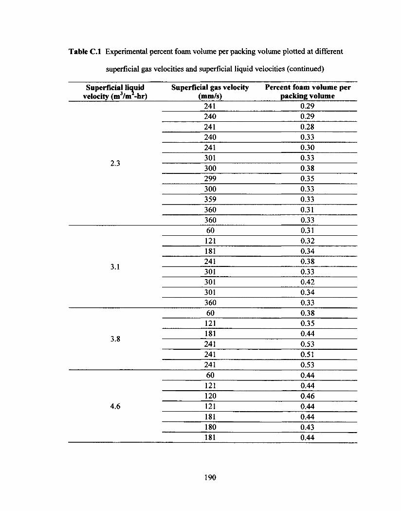
Table C.1 Experimental percent foam volume per packing volume plotted at different
superficial gas velocities and superficial liquid velocities (continued)
Superficial liquid velocity (m3/m2-hr)
2.3
Superficial gas velocity (minis)
241
Percent foam volume per packing volume
0.29 240 0.29 241 0.28 240 0.33 241 0.30
301 0.33 300 0.38 299 0.35 300 0.33 359 0.33
360 0.31 360 0.33
3.1
60 0.31 121 0.32 181 0.34 241 0.38 301 0.33 301 0.42 301 0.34 360 0.33
3.8
60 0.38 121 0.35 181 0.44 241 0.53 241 0.51 241 0.53
4.6
60 0.44 121 0.44 120 0.46 121 0.44 181 0.44 180 0.43 181 0.44
190
Table C.l Experimental percent foam volume per packing volume plotted at different
superficial gas velocities and superficial liquid velocities (continued)
Superficial liquid velocity (m3/m -hr)
Superficial gas velocity (mm/s)
Percent foam volume per packing volume
241 0.29 240 0.29 241 0.28 240 0.33 241 0.30
2.3 301 0.33
2.3 300 0.38 299 0.35 300 0.33 359 0.33 360 0.31 360 0.33 60 0.31 121 0.32 181 0.34
3.1 241 0.38
3.1 301 0.33 301 0.42 301 0.34 360 0.33 60 0.38 121 0.35
3.8 181 0.44
3.8 241 0.53 241 0.51 241 0.53 60 0.44 121 0.44 120 0.46
4.6 121 0.44 181 0.44
o
00
0.43 181 0.44
190

Table C.1 Experimental percent foam volume per packing volume plotted at different
superficial gas velocities and superficial liquid velocities (continued)
Superficial liquid Superficial gas velocity Percent foam volume per velocity (m3/m -hr) (mm/s) packing volume
241 0.55
4.6 241 0.53 241 0.60
241 0.53
191
Table C.l Experimental percent foam volume per packing volume plotted at different
superficial gas velocities and superficial liquid velocities (continued)
Superficial liquid velocity (m3/m -hr)
Superficial gas velocity (mm/s)
Percent foam volume per packing volume
241 0.55
4.6 241 0.60
4.6 241 0.53 241 0.53
191
Related Documents