NOVEMBER 2008 - Brookings · PDF fileNovember 2008 Technological ... a strict quantity-based mechanism (i.e. a fixed ... under the condition that such proposals contain explicit mechanisms

NOVEMBER 2008 ESI Working Paper 08-02

TECHNOLOGICAL SCARCITY, COMPLIANCE FLEXIBILITY AND

THE OPTIMAL TIME PATH OF

EMISSIONS ABATEMENT

Bryan K. Mignone

Brookings Energy Security Initiative

Working Paper 08-02

November 2008

Technological Scarcity, Compliance Flexibility and the Optimal Time Path of Emissions

Abatement

Bryan K. Mignone1,2*

1Foreign Policy Program, The Brookings Institution, Washington, D.C., USA

2 Centre for Applied Macroeconomic Analysis, The Australian National University, Canberra, Australia

This working paper is identical to Centre for Applied Macroeconomic Analysis Working Paper 36/2008 available at http://cama.anu.edu.au/publications.asp. The author thanks Richard Richels of the Electric Power Research Institute for making available the MERGE model code. In addition, the author acknowledges helpful comments from Paul Higgins. * Corresponding author's E-mail: [email protected]

Technological Scarcity, Compliance Flexibility and the Optimal Time Path of Emissions Abatement

Abstract

The overall economic efficiency of a quantity-based approach to greenhouse gas

mitigation depends strongly on the extent to which such a program provides opportunities

for compliance flexibility, particularly with regard to the timing of emissions abatement.

Here I consider a program in which annual targets are determined by choosing the

optimal time path of reductions consistent with an exogenously prescribed cumulative

reduction target and fixed technology set. I then show that if the availability of low-

carbon technology is initially more constrained than anticipated, the optimal reduction

path shifts abatement toward later compliance periods. For this reason, a rigid policy in

which fixed annual targets are strictly enforced in every year yields a cumulative

environmental outcome identical to the optimal policy but an economic outcome worse

than the optimal policy. On the other hand, a policy that aligns actual prices (or

equivalently, costs) with expected prices by simply imposing an explicit price ceiling

(often referred to as a "safety valve") yields the opposite result. Comparison among these

multiple scenarios implies that there are significant gains to realizing the optimal path but

that further refinement of the actual regulatory instrument will be necessary to achieve

that goal in a real cap-and-trade system.

Keywords: Environmental regulation; climate policy; energy modeling.

1

1. Introduction

Article 2 of the Framework Convention on Climate Change (UNFCCC) states that the

ultimate objective of climate policy is "stabilization of greenhouse gas concentrations in

the atmosphere at a level that would prevent dangerous anthropogenic interference

(DAI) with the climate system" (UNFCCC, 1992). Although the exact meaning of DAI

remains the subject of some controversy (O'Neill and Oppenheimer, 2002), a growing

body of scientific literature suggests that global targets in the 450-550 ppm range (and

perhaps even lower) will be necessary to avoid a significant risk of dangerous and

irreversible damage (IPCC, 2007). Achieving the most stringent of these targets would

require a sustained, global reversal of emissions growth within the next several years,

while achieving the more modest targets would likely require such a reversal within the

next one or two decades, depending on how quickly mitigation proceeds once the

growth in emissions is reversed (Mignone et al., 2008).

Because atmospheric stabilization will require a continuous mitigation effort

over the next century and beyond, a common element of policies informed by this

paradigm is the preference for an explicit set of mandated targets and timetables.

Although the concept of stabilization is poorly defined in the national context (since

action by any one country alone cannot yield stabilization), national-level policies may

nonetheless be viewed as consistent with stabilization if the relative domestic reductions

are comparable to the relative reductions required globally (WRI, 2008). These

considerations explain the tendency of the scientific and environmental establishment to

advocate for a system of national caps, ultimately coordinated through international

negotiation.

The economics community has had a more difficult relationship with the idea of

quantity-based mechanisms in the climate policy context, largely because economists

tend to see economic efficiency (realized through policy instruments that promote

2

compliance flexibility) as the most important objective in sound policymaking (e.g.

Aldy et al., 2003). By this standard, a strict quantity-based mechanism (i.e. a fixed

schedule of caps) is relatively inefficient, because it lacks "when-flexibility" or the

ability for regulated entities to shift their compliance obligations across time in response

to real market conditions. The extra effort required to make quantity-based systems

economically efficient, combined with the arguable assumption that the slope of the

marginal damage function is less steep than the slope of the marginal cost function in

the carbon abatement context, has led many economists to favor a carbon tax over a

cap-and-trade system (e.g. Newell and Pizer, 2002).

Despite this theoretical preference for price-based regulation, economists have

generally supported cap-and-trade proposals when they have emerged in the political

arena, under the condition that such proposals contain explicit mechanisms to facilitate

compliance flexibility and overall economic efficiency. Generally speaking,

mechanisms to promote flexibility in the timing of compliance must account for two

contingencies: (1) the possibility that initial targets are not stringent enough with respect

to later targets, in which case the optimal path would require shifting abatement toward

the present, and (2) the possibility that initial targets are too stringent with respect to

later targets, in which case the optimal path would require shifting abatement toward the

future.

The first of these concerns is generally easy to address by allowing firms to bank

permits for later use. Because firms do not have unilateral incentives to overcomply

beyond the optimal amount, there is no reason to place further restrictions on the

quantity of permits a firm may bank in any given year or on the size of the total bank of

permits it may accumulate. Indeed, the existence of an accumulated allowance bank on

the part of regulated industry may actually enhance the political constituency in support

3

of the long-run continuity of the system, because banked permits will only be valuable

if the program remains viable in the future (c.f. McKibbin and Wilcoxen, 2008).

The second concern is more difficult to resolve. In theory, one could allow

unlimited borrowing in the same way that one allows unlimited banking. In a world

with perfect foresight and perfect regulatory certainty, firms would borrow the optimal

number of permits when responding to actual market conditions. However, in the real

world, if firms have imperfect information about the future, doubts about the ability of

regulators to enforce long-term targets, or concerns about the continuity of the system

itself, they may borrow more than the optimal amount, thereby exacerbating the risk of

future default. Moreover, if such defaults do occur (or appear imminent), regulators may

face pressure to revise the reduction targets, leading to the paradoxical conclusion that

the more one tries to encourage the optimal outcome (by enhancing compliance

flexibility), the more likely it is that the program will in fact fail to achieve that optimal

outcome (because the cumulative target will be exceeded to account for defaults).

The problems that surround borrowing suggest several possible responses. First,

one could prohibit borrowing altogether. This would be the recommended course of

action if the efficiency gains from additional compliance flexibility were determined to

be small relative to the risk-adjusted costs associated with the possibility of default.

Another alternative would be to implement a price ceiling (known as a "safety valve")

that would cap the price of CO2 in the permit market (Jacoby and Ellerman, 2004;

McKibbin and Wilcoxen, 2004; Pizer, 2002; Roberts and Spence, 1976). If the safety

valve price mirrored the expected price path, then it would be triggered only if the

compliance obligation in a given year turned out to be more onerous than anticipated

when the reduction path was codified into an annual reduction schedule. In this way, the

conditions under which undercompliance would occur under a safety valve would be

identical to the conditions under which undercompliance would occur in a more

4

conventional specification of borrowing. The critical difference between a safety valve

and borrowing per se is that the former would not require borrowed emissions to be

repaid in later years. This outcome might be acceptable if the cumulative environmental

target were ultimately regarded as flexible but could be far more problematic if the

cumulative target were decided through prior negotiation. In that case, the mechanism

proposed to enhance flexibility – to the extent that it threatened a fragile political

coalition over targets – could once again jeopardize the system itself.

With these considerations as a backdrop, we examine, in the remainder of this

paper, the economic and environmental implications of several policies designed to

capture the different ways in which compliance flexibility could be implemented in a

real cap-and-trade system. In particular, we use a well-known computable model to

show that if low-carbon technology turns out to be more scarce than anticipated,

inflexible annual targets would drive up the economic costs of mitigation well beyond

the costs of a policy with optimal borrowing. The value of this difference provides one

measure of the benefits of enhancing compliance flexibility that can be compared to any

proposed measure of the risk-adjusted costs of default.

While the benefits of providing flexibility and achieving the when-efficient

outcome are significant, we show that attempting to realize these benefits by applying a

conventional safety valve (to align the actual cost of the policy with the anticipated cost)

threatens the cumulative environmental integrity of the program by an amount that is

likely to jeopardize the political coalition around targets. A safety valve policy may

even be economically suboptimal if the cumulative target is decided through a separate

balancing of costs and benefits and if the emissions overages are sufficient to drive

down the level of avoided damages (benefits). Together, these simulations suggest that

there are real economic and environmental gains to developing a credible policy

5

instrument that can achieve a when-efficient response to a cumulative emissions

reduction target.

2. Model Description and Baseline Results

In order to quantitatively evaluate the tradeoff between economic efficiency and

environmental integrity under cap-and-trade, we make use of the MERGE model, a

well-documented computable general equilibrium (CGE) model of the energy-economic

system that combines a top-down specification of the macroeconomy with a bottom-up

specification of the energy sector (Manne et al., 1995). In the simplified configuration

used for this study, we reduce the number of distinct world regions in the model to one

(the United States) and the number of carbon abatement technologies to two, one

deployable in the power sector and one deployable in the fuels sector.

In the power sector, this single aggregate technology is meant to represent the

larger set of low-carbon technologies like coal equipped with carbon capture and

storage (CCS), advanced nuclear, wind, solar and geothermal, among others. Both

aggregate abatement technologies are assumed to be available at a marginal (levelized)

cost premium of $50 per ton CO2, but because the large-scale availability of these

sources remains the subject of some debate, the time at which they are assumed to be

available for deployment is one of the adjustable parameters in this study, along with

the details of the regulatory system itself. In addition to technology substitution, the

model also includes an explicit demand response to price (over and above autonomous

improvements in energy efficiency), with a long-run elasticity of 0.3. Together these

two features allow the model to capture, in an aggregate manner, both supply and

demand-side responses to carbon mitigation policy.

Model simulations begin in 2010, with (forecast) data in that year supplied by

the US Energy Information Administration (EIA, 2008). Under business-as-usual

6

conditions (no policy constraints), economic output (GDP) in the US starts in 2010 at

about 12.5 trillion USD and grows at approximately 2.4% per year to 32 trillion USD in

2050, consistent with the EIA growth forecast over the 2006-2030 horizon. Over the

same period, total energy consumption (or more precisely, the total energy contained in

the fuels used for such consumption) grows from 110 EJ in 2010 to 143 EJ in 2050,

representing an annual growth of energy demand of approximately 0.7%, which is also

broadly consistent with EIA projections through 2030. The difference between the

growth rate of economic output and the growth rate of energy consumption provides a

measure of the rate of autonomous energy efficiency improvement. Using the numbers

above, we find that the overall energy intensity of the economy decreases by about 1.7%

per year, a trend that is assumed to continue in the future with or without explicit policy

intervention.

The future fuel mix under business-as-usual also continues to reflect historical

trends, with coal dominating the power sector and oil dominating the fuels sector. Over

the course of the (baseline) simulation, coal, natural gas, nuclear and renewables

(including hydropower) account for approximately 51%, 17%, 20% and 11% of energy

supplied in the power sector, respectively, whereas oil, natural gas, coal and renewables

account for 65%, 28%, 3.3% and 4.4% of energy supplied in the fuels sector,

respectively. Because consumption of all fossil fuels continues to grow under business-

as-usual, CO2 emissions also continue to rise, from 6.0 Pg CO2 in 2010 to 8.0 Pg CO2 in

2050, an increase of approximately 0.7% per year. The business-as-usual emissions

trend is shown by the black markers in panel (a) of Figure 1.

3. Policy Simulations

The energy system response to applied CO2 targets can be modeled in a number of

different ways. Typically, modelers working within the intellectual framework of

constrained dynamic optimization have preferred to specify a constraint on cumulative

7

emissions over a predetermined period of time, or similarly, a constraint on the ultimate

atmospheric CO2 concentration.1 In either case, the imposition of a single aggregate

constraint, as opposed to an ordered set of annual constraints, allows the model to

endogenously solve for the economically efficient (least-cost) time path of abatement,

thus providing a trajectory of annual targets that can be used to further develop concrete

policy recommendations. However, to the extent that annual targets have already been

codified in legislative or regulatory language, this approach essentially assumes full

when-flexibility during compliance (i.e. unlimited banking and borrowing by regulated

entities), an assumption whose importance will be analyzed in greater detail below.

To make this problem as concrete and as simple as possible, we begin by

imposing a cumulative emissions target equal to the sum of annual targets (between

2012-2050) specified in the Lieberman-Warner Climate Security Act, a bill that was

1 If CO2 were a perfect stock pollutant, so that the total atmospheric stock equalled the sum of prior

annual inflows, a cumulative emissions constraint would be identical to a concentration stabilization

constraint. In fact, CO2 is gradually removed from the atmosphere by natural ocean and land processes

(see, e.g., Mignone et al., 2008), meaning that the annual net inflow (and resulting atmospheric stock) is

determined by a more complex balance between sources and sinks. Nevertheless, the basic qualitative

insight that the underlying environmental objective depends strongly on the cumulative emissions release,

and less so on the details of the trajectory, remains valid for the scenarios considered in this study.

8

considered on the floor of the US Senate in June 2008.2 The model-derived optimal

time path of emissions abatement under "core technology" assumptions (that is,

assuming both abatement technologies are available for deployment from the start of the

simulation) is shown by the dark blue markers in panel (a) of Figure 1. It is worth

noting that the emissions constraint is sufficiently stringent to require an immediate

reversal in emissions growth, at least when technology to enable these reductions is

assumed to be readily available from the start.

We next apply the same cumulative emissions constraint to a world in which the

introduction of low-carbon technology is delayed by 10 years (i.e. until after 2020). The

adjusted optimal emissions path is shown by the green markers in panel (a) of Figure 1.

Not surprisingly, the emissions reductions in this case are delayed with respect to the

core technology case, with less stringent reductions in early years and more stringent

reductions in later years. The shift in abatement toward later compliance periods in the

delayed technology case is most apparent in panel (b) of Figure 1, which shows the

difference in annual emissions relative to the core technology case. The difference is

positive for approximately the first half of the simulation and negative for the

remainder. By design, the integral of this difference over the entire simulation must be

equal to zero in order to satisfy the cumulative emissions constraint, which is identical

in the core and delayed technology policy cases.

2 We take the numerical targets from S. 3036, the Boxer substitute to the Committee-reported version of

the Lieberman-Warner bill (S. 2191). Full text of these bills is available at http://www.thomas.gov. In this

study, we make the additional assumption that emissions from covered sources are equivalent to energy-

related CO2 emissions, allowing us to apply the targets verbatim. For more detailed economic analyses of

this legislation, see the reports by the US Environmental Protection Agency (available at

http://www.epa.gov) and the US Energy Information Administration (available at

http://www.eia.doe.gov).

9

If low-carbon technology is assumed to be widely available during the

development of a regulatory program, then policymakers will tend to codify the optimal

path from the core technology policy case into binding annual targets (blue markers in

Figure 1). If low-carbon technology later turns out to be less widely available than

anticipated, then the optimal response to such technological scarcity (green markers in

Figure 1) can only be realized if regulated entities are allowed to borrow permits from

future periods. As discussed above, implementing such provisions in the context of a

real cap-and-trade system is fraught with difficulty, because borrowing enhances the

risk of future default and jeopardizes the viability of the underlying program.

To address these issues, we have examined two additional policy cases – a safety

valve case and a no-borrowing case – intended to simulate possible real-world responses

to the default risk problem. The addition of a safety valve essentially institutionalizes a

limited amount of default by releasing regulated entities from the obligation to repay

borrowed permits. On the other hand, the elimination of borrowing is a rather blunt

response to the default risk problem that eliminates the risks associated with a particular

mechanism by eliminating the mechanism itself. In effect, these two policy cases

represent two extreme responses to the default risk problem, with the first sanctioning

some amount of future default and the latter adopting a draconian precautionary

approach toward default risk.

Both of these additional cases are variations on the delayed technology policy

case considered above, in the sense that both assume that the entry of low-carbon

technology is delayed by 10 years. The first is modeled by applying the annual targets

derived from the core technology policy case together with a safety valve that caps

permit prices in each year at the corresponding value from the core technology case.

This particular setup reflects the assumption in this paper that the purpose of a safety

valve is to align actual prices with expected prices during the initial phases of a new

10

regulatory program.3 Ultimately, a safety valve enhances compliance flexibility by

allowing emissions targets to be exceeded in the early years when technology is more

scarce than initially anticipated, but it does so without requiring such "borrowed"

emissions to be paid back in later periods, thus favoring compliance flexibility at the

expense of environmental integrity.

The second additional policy scenario – the no-borrowing case – is essentially

the mirror image of the safety valve case, in the sense that it represents an extreme

attachment to (annual) environmental goals at the expense of compliance flexibility.

This scenario is modeled by applying the annual targets derived from the core

technology policy case together with an additional constraint that the cumulative bank

of stored permits must never drop below zero. Under this condition, emissions in a

given year may only rise above the prescribed annual target when regulated entities are

drawing down an existing accumulated bank of allowances resulting from

overcompliance in an earlier period.

The simulated emissions trajectories for the two additional policy cases are

shown by the red and light blue markers, respectively, in panel (a) of Figure 1, and the

annual differences from the core technology policy case are shown in panel (b) of

3 Of course, other assumptions about the purpose of a safety valve are possible. While the US policy

discussion has often focused on the threat posed by near-term technological scarcity, a safety valve could

also be used to protect against other contingencies, like shorter-term volatility unrelated to technology

(e.g. swings in emissions driven by the business cycle) or the possibility that long-run mitigation costs are

simply higher, on average, than policymakers anticipate or would be willing to pay. Note that the former

problem can be addressed through other forms of compliance flexibility, like borrowing, while the latter

cannot. Some will argue that this versatility provides an additional reason to consider the safety valve

over alternative flexibility mechanisms, while others will view a long-term mismatch between expected

and actual prices as reason to revisit the underlying details of the program, including the strategic targets.

11

Figure 1. Emissions from the safety valve case roughly track emissions of the delayed

technology policy case (green markers) during the 10-year period when low-carbon

technology is scarce, but significantly exceed emissions from the delayed technology

case in later years. In effect, because payback is not required, the reductions do not

steepen sufficiently in later years to make up the early overages, meaning that the

cumulative emissions in the safety valve case significantly exceed the cumulative

emissions associated with the applied targets, when integrated over the entire 40-year

window. The magnitude of this difference (~20 Pg CO2) is equal to the area under the

red markers in panel (b) of Figure 1.

Finally, under the no-borrowing case, regulated entities slightly overcomply (i.e.

bank permits) in the very earliest periods and then draw down this bank in the periods

immediately following, as shown by the light blue markers in panels (a) and (b) of

Figure 1. While the difference in any given year between the applied targets and the

actual emissions is relatively small (to first order, the emissions simply track the

emissions in the core technology policy case), it is worth exploring this deviation,

because banking (overcompliance) is counterintuitive in a scenario in which the targets

are extremely strict. The result is actually considerably less perplexing when one

examines the simulated allowance prices for these scenarios, which we consider next.

Panel (c) of Figure 1 shows the simulated allowance prices for the four

scenarios described above. In the core technology case, the allowance price begins at

~$23 per ton CO2 in 2011 and rises at the interest rate (~6%) to almost $200 per ton in

2050. It is worth noting that, even though advanced technology is deployed

immediately, the initial carbon price is lower than the assumed technology crossover

price ($50 per ton CO2), because the price of a permit in any given year represents the

opportunity cost associated with a marginal unit of emissions. When the climate

constraint is applied as an upper bound on the allowable cumulative emissions, the

12

opportunity cost of a unit of emissions in the first period is the discounted value of an

additional unit of abatement in a future period, which must always be less than the

instantaneous value ($50 in this case) (Mignone, 2008).

When low-carbon technology is initially scarce, the optimal transition path shifts

abatement toward later periods. Again, because the price of a permit in the first year

represents the opportunity cost of an additional unit of future abatement, the price in the

first year must reflect the discounted value of this future action. That price is the sum of

the technological crossover price and the additional adjustment cost associated with the

more rapid decline of emissions (and energy capital) in later years. In other words, the

allowance price path in the delayed technology policy case sits above the allowance

price path for the core scenario (starting in the former at about $35 per ton CO2) because

there is a premium associated with the steeper reductions mandated by the early deferral

of abatement.

Having considered the full-flexibility cases, it is worth examining the simulated

allowance price trajectories in the remaining two policy scenarios. The price path under

the safety valve case is reasonably intuitive. Because the applied price ceiling reflects

the prices required to generate the prescribed abatement path when low-carbon

technology is widely available, it underestimates the prices required to support the same

level of abatement when technology is more limited. For this reason, the safety valve

binds in each period, and the allowance prices remain pegged to the values associated

with the safety valve.

In the no-borrowing case, the prices start very high (at ~$100 per ton CO2) but

fall dramatically in later periods to values consistent with the core technology case. The

very high initial prices result from the fact that borrowing is prohibited at a time when

technology is extremely scarce, meaning that the required abatement must come from

demand destruction. However, this does not explain the observed banking in early

13

periods. Indeed, the apparent overcompliance seems to suggest that the same targets

could be met at lower carbon prices, and thus lower overall economic cost. However,

this conclusion neglects the full extent of the prohibition on borrowing. While lower

prices would be consistent with the targets in the very earliest periods, it would drive up

emissions in the periods immediately following, leading to cumulative emissions

overages that would exceed the earlier amount banked, thus violating the no-borrowing

constraint. In other words, prices lower than those observed would not generate a bank

sufficiently large to cover the overages that immediately follow.

Finally, changes in economic output for each of the scenarios are shown in panel

(d) of Figure 1. In the core technology case and in the safety valve case, the relative

loss of GDP relative to business-as-usual increases over the simulation to a maximum of

about 1.5% annually. In the delayed technology case, economic losses peak at ~2% at

the end of the 10-year period in which technology is constrained (i.e. in 2020), while in

the no-borrowing case, the economic losses reach a maximum of ~3% over that period.

The difference between these latter two scenarios – that is, between the optimal

borrowing case (green markers) and the no-borrowing case (light blue markers) –

provides one measure of the economic benefit of compliance flexibility.

Because the availability of low-carbon technology is so uncertain, Figure 2

shows the sensitivity of the environmental and economic results to assumptions about

the time at which low-carbon technology enters the market, with the point of entry

varying between 2010 (i.e. technology available immediately) and 2030 (i.e. 20 year

delay before technology is available). Each point in these figures represents an

aggregate result from a separate model simulation. Panels (a) and (b) of Figure 2 show

the (undiscounted) cumulative GDP loss, relative to the core technology optimum for

the 2010-2030 and 2010-2050 periods, respectively. A quick inspection of these figures

reveals that, while the magnitude of the economic loss increases with the number of

14

years until low-carbon technology is introduced, the relative ranking of the different

policies is robust to such assumptions and to the period over which costs are integrated.

As one might expect, the no-borrowing scenarios are always the most expensive, the

safety valve scenarios are always the least expensive and the optimal borrowing

scenarios are always less expensive than the former but more expensive than the latter.

Panels (c) and (d) of Figure 2 show the cumulative emissions overages, relative

to the core technology optimum, for the 2010-2030 and 2010-2050 periods,

respectively. Over the near-term (2010-2030), the overages in panel (c) vary inversely

with the costs in panel (a), in the sense that the scenarios with the greatest near-term

emissions overages (safety valve scenarios) are the ones achieved at least cost, while the

scenarios with the lowest near-term emissions overages (no-borrowing scenarios) are

the ones achieved at greatest cost. Again, as one might expect, the scenarios with near-

term emissions overages in between the other two (the optimal borrowing scenarios)

achieve costs that also fall in between the other two sets of scenarios.

We find similar results in panel (d), with one critical difference, namely that the

emissions overages associated with the optimal borrowing scenarios are eliminated

when the period of integration is extended to 2050. Thus, in comparing panels (d) and

(b), we find the same inverse relationship between costs and emissions in the safety

valve and no-borrowing scenarios, but an interesting and important asymmetry in the

optimal borrowing scenarios. By design, the cumulative emissions releases are always

identical to the no-borrowing emissions releases (which, in turn, are equal to the release

from the core technology optimal case) but the costs of the optimal borrowing scenarios

are significantly lower than the no-borrowing scenarios because of the added flexibility

in the former. To the extent that the long-term (as opposed to near-term) cumulative

emissions release is a more relevant measure of the benefit of the policy (so that the

benefit is the same in each case), the difference in cost provides a measure of the

15

efficiency gain (in dollar terms) associated with realizing the optimal time path of

abatement.

4. Conclusions

Ultimately, decisions about the design of a greenhouse gas regulatory program will

hinge on judgments about the proper tradeoff between environmental integrity and

economic certainty in the climate policy context, together with additional judgments

about the practical and political viability of the instruments designed to achieve such a

balance. This paper primarily sheds light on the first of these two questions. In

particular, the simulations discussed here suggest that if the true objective of climate

policy is to achieve a particular cumulative amount of emissions abatement at least cost,

then a policy instrument that allows regulated entities to endogenously shift their

compliance obligation across time significantly outperforms instruments in which such

compliance flexibility is constrained or imperfect. Our results therefore provide some

measure of the environmental and economic benefit of realizing compliance flexibility.

The four simulations discussed in this study are summarized compactly in Table

1. A close inspection of these results suggests that when regulated entities are allowed

to shift abatement across time in response to actual technological circumstances, the

cumulative environmental goals of the program can be preserved with only modest

increases in the overall economic cost (compare the core technology and delayed

technology cases). However, if regulated entities must instead achieve strict annual

goals in the face of severe technological scarcity, then the costs of the program rise

dramatically to satisfy the very difficult early targets, while the added benefit is

negligible given that the cumulative target remains unchanged relative to the delayed

technology optimum. Finally, if a safety valve is applied in lieu of borrowing, then

actual costs track expected costs over the duration of the simulation, but the cumulative

16

environmental target is exceeded by an amount that is likely to jeopardize the political

coalition around targets and potentially the environmental benefit itself.

The magnitude of the efficiency gain associated with optimal borrowing (and

more generally, the differences between scenarios) varies with assumptions about the

availability of low-carbon technology. However, the existence of such a benefit is

robust to the technology assumptions, and on a relative basis, the gain is always

significant, with a reduction in total (cumulative cost) of perhaps 40% relative to the no-

borrowing case. This finding suggests that there are real economic gains to adopting

policies that provide mechanisms to achieve flexibility in the timing of abatement.

Given the magnitude of this potential efficiency gain, the second question about

feasibility is obviously paramount. For reasons discussed at greater length earlier,

borrowing is difficult to implement because it exposes the trading system to significant

default risk. Some recent analyses have suggested ways to mitigate default risk by

incorporating specific features of the safety valve (i.e. price triggers) into mechanisms

that would preserve the cumulative environmental integrity of the system. One such

example is a "reserve auction" that would inject a limited number of permits "borrowed"

from future compliance periods into earlier periods, as a supplement to the primary

permit distribution mechanism (Murray et al., 2008). Future work will need to further

evaluate such mechanisms to determine whether borrowing can in fact be implemented

in ways that enable regulated entities (and thus consumers) to realize the efficiency

benefits associated with compliance flexibility, and if so, to determine which of these

mechanisms would be optimal in the context of a real regulatory program.

17

Figure 1

Environmental and economic diagnostics for the four simulations discussed in the text.

Panel (a) shows CO2 emissions as a function of time, and panel (b) shows differences in

annual emissions from the core technology policy case as a function of time, with

positive values representing undercompliance and negative values representing

overcompliance with respect to the core technology policy case. Panel (c) shows

simulated allowance prices as a function of time, and panel (d) shows economic losses

as a function of time, calculated as the relative GDP difference between each policy

scenario and the business-as-usual path.

18

Figure 2

Environmental and economic diagnostics for a series of simulations examining the

sensitivity to the technology assumptions in the model. Panel (a) shows the cumulative

(undiscounted) GDP loss (relative to the core technology optimum case) between 2010-

2030 as a function of the year in which low-carbon technology is first assumed to be

available, while panel (b) shows the same results integrated over the 2010-2050 period.

Panel (c) shows the cumulative CO2 emissions overage (relative to the core technology

case) between 2010-2030 as a function of the technology entry date, while panel (d)

shows the same results integrated over the 2010-2050 period.

19

SCEN TECH

AVAIL. EMISSIONS

CONSTRAINT

INITIAL PRICE ($/ton CO2)

EMISSIONS REDUCTION FROM BAU

(Pg CO2)

GDP REDUCTION FROM BAU

(Trillion USD)

2010-2030

2010-2050

2010-2030

2010-2050

CORE Full set Optimal path to cumulative LW

Target 23 29 125 3.2 10.3

DELAY Entry

delayed by 10 yrs

Optimal path to cumulative LW

target 35 24 125 4.8 12.8

SAFETY VALVE

Entry delayed

by 10 yrs

Annual targets from CORE; Full Banking; SV with prices from CORE

23 19 106 3.3 10.5

NO BORROW

Entry delayed

by 10 yrs

Annual targes from CORE; Full Banking; No Borrowing

106 29 125 7.4 16.4

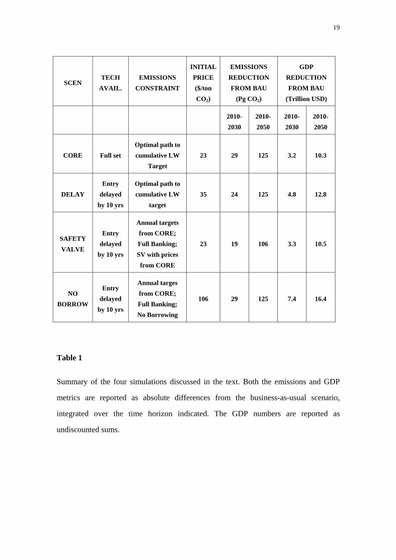
Table 1

Summary of the four simulations discussed in the text. Both the emissions and GDP

metrics are reported as absolute differences from the business-as-usual scenario,

integrated over the time horizon indicated. The GDP numbers are reported as

undiscounted sums.

20

References

Aldy J E, Barrett S, Stavins R N. Thirteen plus one: A comparison of global climate

policy architectures. Climate Policy 2003; 3; 373-397.

EIA. Annual Energy Outlook 2008. Energy Information Administration, Washington,

D.C. Available at http://www.eia.doe.gov.

IPCC. Climate Change 2007: Synthesis Report. Contribution of Working Groups I, II

and III to the Fourth Assessment Report of the Intergovernmental Panel on Climate

Change (Eds: Core Writing Team, Pachauri, R K and Reisinger, A). Geneva,

Switzerland, 104 pp.

Jacoby H D, Ellerman A D. The safety valve and climate policy. Energy Policy 2004;

32; 481-491.

Manne A, Mendelsohn R, Richels R. A model for evaluating regional and global effects

of GHG reduction policies. Energy Policy 1995; 23; 17-34.

McKibbin W J, Wilcoxen, P J. Estimates of the costs of Kyoto: Marrakesh versus the

McKibbin-Wilcoxen blueprint. Energy Policy 2004; 32; 467-479.

McKibbin W J, Wilcoxen P J. Building on Kyoto: Towards a realistic global climate

agreement. Brookings Energy Security Policy Brief 08-01, October 2008.

Mignone B K, Socolow R H, Sarmiento J L, Oppenheimer M. Atmospheric stabilization

and the timing of carbon mitigation. Climatic Change 2008; 88; 251-265.

Mignone B K. Prices in emissions permit markets: The role of investor foresight and

capital durability. Centre for Applied Macroeconomic Analysis Working Paper

31/2008. The Australian National University. Available at http://cama.anu.edu.au.

21

Murray B C, Newell R G, Pizer W A. Balancing cost and emissions certainty: An

allowance reserve for cap-and-trade. Nicholas Institute Working Paper 08-03, Duke

University. Available at http://www.nicholas.duke.edu.

Newell R G and Pizer W A. Regulating stock externalities under uncertainty. Journal of

Environmental Economics and Management 2002; 45; 416-432.

O'Neill B C, Oppenheimer M. Dangerous climate impacts and the Kyoto Protocol.

Science 2002; 296; 1971-1972.

Pizer W. Combining price and quantity certainty controls to mitigate global climate

change. Journal of Public Economics 2002; 85; 409-434.

Roberts, M J, Spence M. Effluent charges and licenses under uncertainty. Journal of

Public Economics 1976; 5; 193-208.

UNFCCC. United Nations Framework Convention on Climate Change 1992. Text

available at http://unfccc.int.

WRI. Comparison of Legislative Climate Change Targets, September 9, 2008. World

Resources Institute, Washington, D.C. Text available at http://www.wri.org.