Novel Flexible Statistical Methods for Missing Data Problems and Personalized Health Care by Yilun Sun A dissertation submitted in partial fulfillment of the requirements for the degree of Doctor of Philosophy (Biostatistics) in The University of Michigan 2019 Doctoral Committee: Associate Professor Lu Wang, Chair Assistant Professor Peisong Han Research Associate Professor Matthew J. Schipper Associate Professor Emily Somers

Welcome message from author
This document is posted to help you gain knowledge. Please leave a comment to let me know what you think about it! Share it to your friends and learn new things together.
Transcript

Novel Flexible Statistical Methods for MissingData Problems and Personalized Health Care
by
Yilun Sun
A dissertation submitted in partial fulfillmentof the requirements for the degree of
Doctor of Philosophy(Biostatistics)
in The University of Michigan2019
Doctoral Committee:
Associate Professor Lu Wang, ChairAssistant Professor Peisong HanResearch Associate Professor Matthew J. SchipperAssociate Professor Emily Somers


ACKNOWLEDGEMENTS
I want to extend thanks to my instructors, peer students, friends, and family, who so
generously contributed to the work presented in this thesis.
First and foremost, I am indebted to my advisor, Lu Wang. Lu is always generous
with her time, she is always a good listener, and she always provides insightful advice.
Her valuable suggestions, comments, and guidance encourage me to stay persistent
towards my goals. Lu is an inspiring advisor in many ways, and her guidance has
been significantly helping me gain knowledge, develop research interests, grow as a
research scholar, as well as balance work and family. This dissertation would not have
been possible without the consistent guidance, encouragement, and support from Lu.
I want to thank Matthew Schipper, for supervising my GSRA research, supporting
my Ph.D. study, and serving as my dissertation committee member. Matt has been
very understanding and supportive since my first day working with him. He has been
giving me both independence and guidance, teaching me to conduct collaborative
research effectively and helping me gain valuable experience in developing statistical
tools for exciting and meaningful radiation oncology applications.
I am also grateful to the rest of my dissertation committee members, Peisong Han, and
Emily Somers. I collaborated with Peisong in my first thesis project and benefited
greatly from his tremendous passion for research, broad knowledge, and insightful
comments. I am thankful to Emily for agreeing to serve on my dissertation committee
ii

on such short notice, and her invaluable insights and suggestions helped me improve
my thesis.
I want to express my gratitude to Jeremy Taylor. Jeremy supervised my research in
the summer even before I officially started my Ph.D. study, and has always been very
supportive. His excellent guidance and mentorship helped me get on the right track
and realize my research interest. Moreover, his rigorous attitude toward scholarship
has dramatically influenced my work ever since.
Thanks are also due to the faculty, staff, and peer students in the Department of
Biostatistics, University of Michigan. Also, I am grateful to my collaborators from
Michigan Medicine.
Special thanks to my beloved family members. I want to thank my mom, Xi Wang,
without her selfless support, I would not be able to make this accomplishment. I also
want to thank my wife, Yang Jiao, and my two lovely kids, Joanna and Lucas. I
would like to thank them for all the support, joy, and love. I am fortunate to have
them in my life.
iii

TABLE OF CONTENTS
ACKNOWLEDGEMENTS . . . . . . . . . . . . . . . . . . . . . . . . . . ii
LIST OF FIGURES . . . . . . . . . . . . . . . . . . . . . . . . . . . . . . . vi
LIST OF TABLES . . . . . . . . . . . . . . . . . . . . . . . . . . . . . . . . vii
LIST OF APPENDICES . . . . . . . . . . . . . . . . . . . . . . . . . . . . ix
ABSTRACT . . . . . . . . . . . . . . . . . . . . . . . . . . . . . . . . . . . x
CHAPTER
I. Introduction . . . . . . . . . . . . . . . . . . . . . . . . . . . . . . 1
II. Multiply Robust Estimation in Nonparametric Regression
with Missing Data . . . . . . . . . . . . . . . . . . . . . . . . . . . 6
2.1 Introduction . . . . . . . . . . . . . . . . . . . . . . . . . . . 62.2 The Proposed Estimator . . . . . . . . . . . . . . . . . . . . . 82.3 Large Sample Properties . . . . . . . . . . . . . . . . . . . . . 13
2.3.1 Multiple Robustness . . . . . . . . . . . . . . . . . . 132.3.2 Asymptotic Distribution and Efficiency . . . . . . . 16
2.4 Simulation Studies . . . . . . . . . . . . . . . . . . . . . . . . 202.5 Data Applications . . . . . . . . . . . . . . . . . . . . . . . . 262.6 Discussion . . . . . . . . . . . . . . . . . . . . . . . . . . . . 28
III. Stochastic Tree Search for Estimating Optimal Dynamic Treat-
ment Regimes . . . . . . . . . . . . . . . . . . . . . . . . . . . . . 31
3.1 Introduction . . . . . . . . . . . . . . . . . . . . . . . . . . . 313.2 Stochastic Tree-based Reinforcement Learning . . . . . . . . . 34
3.2.1 Dynamic Treatment Regimes . . . . . . . . . . . . . 343.2.2 Bayesian Additive Regression Trees . . . . . . . . . 36
iv

3.2.3 Stochastic Tree Search Algorithm . . . . . . . . . . 373.2.4 Implementation of ST-RL . . . . . . . . . . . . . . . 41
3.3 Theoretical Results . . . . . . . . . . . . . . . . . . . . . . . 423.4 Simulation Study . . . . . . . . . . . . . . . . . . . . . . . . . 46
3.4.1 Single-stage Scenarios . . . . . . . . . . . . . . . . . 473.4.2 Two-stage Scenarios . . . . . . . . . . . . . . . . . . 50
3.5 Data Applications . . . . . . . . . . . . . . . . . . . . . . . . 533.6 Discussion . . . . . . . . . . . . . . . . . . . . . . . . . . . . 55
IV. A Flexible Tailoring Variable Screening Approach for Esti-
mating Optimal Dynamic Treatment Regimes in Large Ob-
servational Studies . . . . . . . . . . . . . . . . . . . . . . . . . . 57
4.1 Introduction . . . . . . . . . . . . . . . . . . . . . . . . . . . 574.2 Method . . . . . . . . . . . . . . . . . . . . . . . . . . . . . . 60
4.2.1 Optimal Treatment Regime and Additive Models . . 604.2.2 Back-fitting Algorithm for Sparse Additive Selection 634.2.3 Extension to Multi-stage Setting . . . . . . . . . . . 67
4.3 Simulation Study . . . . . . . . . . . . . . . . . . . . . . . . . 684.3.1 Single-stage Scenarios . . . . . . . . . . . . . . . . . 684.3.2 Two-stage Scenarios . . . . . . . . . . . . . . . . . . 71
4.4 Application . . . . . . . . . . . . . . . . . . . . . . . . . . . . 754.5 Discussion . . . . . . . . . . . . . . . . . . . . . . . . . . . . 78
V. Summary and Future Work . . . . . . . . . . . . . . . . . . . . . 80
APPENDICES . . . . . . . . . . . . . . . . . . . . . . . . . . . . . . . . . . 82
BIBLIOGRAPHY . . . . . . . . . . . . . . . . . . . . . . . . . . . . . . . . 98
v

LIST OF FIGURES
Figure
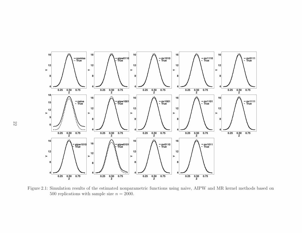
2.1 Simulation results of the estimated nonparametric functions usingnaive, AIPW and MR kernel methods based on 500 replications withsample size n = 2000. . . . . . . . . . . . . . . . . . . . . . . . . . 22
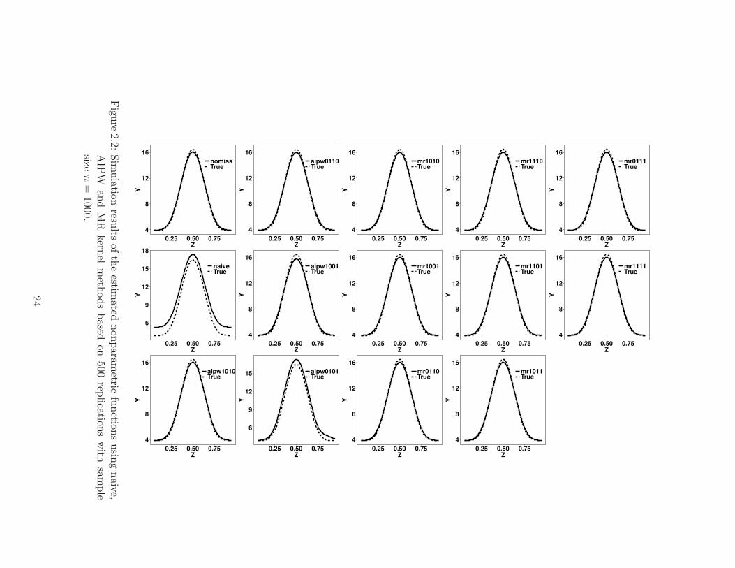
2.2 Simulation results of the estimated nonparametric functions usingnaive, AIPW and MR kernel methods based on 500 replications withsample size n = 1000. . . . . . . . . . . . . . . . . . . . . . . . . . . 24
2.3 The naive and multiply robust KEE estimates of ozone exposure (inppb) on systolic blood pressure. Each vertical tick mark along thex-axis stands for one observation. . . . . . . . . . . . . . . . . . . . 29
4.1 The regularization path calculated for HCC data. The ratio betweenthe two tuning parameters is fixed at λ1/λ2 = 1.5. . . . . . . . . . . 78
vi

LIST OF TABLES
Table
2.1 Simulation results of relative biases, S.E.s and MISEs of the naive,AIPW and MR estimates of θ(z) based on 500 replications. . . . . . 26
3.1 Simulation results for single-stage scenarios I-IV, with 50, 100, 200baseline covariates and sample size 500. The results are averaged over500 replications. opt% shows the median and IQR of the percent-age of test subjects correctly classified to their optimal treatments.EY ∗(gopt) shows the empirical mean and the empirical standard de-viance of the expected counterfactual outcome under the estimatedoptimal regime. . . . . . . . . . . . . . . . . . . . . . . . . . . . . . 49
3.2 Simulation results for two-stage scenarios V-VIII, with 50, 100, 200baseline covariates and sample size 500. The results are averaged over500 replications. opt% shows the median and IQR of the percent-age of test subjects correctly classified to their optimal treatments.EY ∗(gopt) shows the empirical mean and the empirical standard de-viance of the expected counterfactual outcome under the estimatedoptimal regime. . . . . . . . . . . . . . . . . . . . . . . . . . . . . . 52
4.1 Simulation results for single-stage Scenarios I and II based on 500replications. Size: number of interactions selected; TP: number oftrue interactions selected. . . . . . . . . . . . . . . . . . . . . . . . . 71
4.2 Simulation results for single-stage Scenarios III and IV based on 500replications with ρ = 0.2. The methods S-Score, ForMMER, SAS andPAL are implemented using one-versus-all approach. Size: numberof interactions selected; TP: number of true interactions selected. . . 72
4.3 Simulation Results in Two Stage Scenarios V and VI. Size: numberof interactions selected; TP: number of true interactions selected; TP(µ1): number of true interactions between A1 and (X1,11, · · · , X1,15)selected. . . . . . . . . . . . . . . . . . . . . . . . . . . . . . . . . . 74
vii

4.4 Patient Demographics in HCC Study . . . . . . . . . . . . . . . . . 75
4.5 The variable selection results for HCC data. . . . . . . . . . . . . . 77
viii

LIST OF APPENDICES
Appendix
A. Proofs for Chapter II . . . . . . . . . . . . . . . . . . . . . . . . . . . 83
B. Proofs for Chapter III . . . . . . . . . . . . . . . . . . . . . . . . . . . 90
ix

ABSTRACT
Coarsened data, including a broad class of incomplete data structures, are ubiquitous
in biomedical research. Various methods have been proposed when data are coarsened
at random, where it is often required to specify working models for the coarsening
mechanism, or the conditional outcome regression, or both. However, some practical
issues emerge: for example, it is not unusual to have multiple working models that all
fit the observed data reasonably well, or working model specification can be challeng-
ing in the presence of a large number of variables. In this dissertation, we propose
new flexible statistical methods to tackle the challenges mentioned above with two
types of coarsened data: missing data and counterfactual data when optimizing the
dynamic treatment regime (DTR), which is a sequence of decision rules that adapt
treatment to the time-varying medical history of each individual.
In the first project, we develop a multiply robust kernel estimating equations (MR-
KEEs) method for nonparametric regression that can accommodate multiple working
models for either the missing data mechanism or the outcome regression or both.
The resulting estimator is consistent if any one of those models is correctly specified.
When including correctly specified models for both, the proposed estimator achieves
the optimal efficiency within the class of augmented inverse probability weighted
(AIPW) kernel estimators.
In the second project, we develop a stochastic tree-based reinforcement learning
method, ST-RL, for estimating the optimal DTR in a multi-stage multi-treatment set-
ting with data from either randomized trials or observational studies. At each stage,
ST-RL constructs a decision tree by first modeling the mean counterfactual outcomes
via Bayesian nonparametric regression models, and then stochastically searching for
x

the optimal tree-structured regime using a Markov Chain Monte Carlo algorithm.
We implement the proposed method in a backward inductive fashion through multi-
ple decision stages. Compared to existing methods, ST-RL delivers the optimal DTR
with better interpretability and does not require explicit working model specifications.
Besides, ST-RL demonstrates stable and outstanding performance with moderately
high dimensional data.
In the third project, we propose a variable selection technique to screen potential
tailoring variables for estimating the optimal DTR with large observational data.
The proposed method is based on nonparametric sparse additive models and therefore
enjoys superior flexibility. Also, it allows treatments with more than two levels, as well
as continuous doses. In particular, the selection procedure enforces strong heredity
constraint, i.e., the interactions can only be included when both of its main effects
have already been selected.
xi

CHAPTER I
Introduction
Coarsened data (Heitjan, 1993;Gill et al., 1997) are ubiquitous in biomedical research.
The term coarsened data represents a broad class of incomplete data structures,
where the observed data can be viewed as many-to-one functions of complete data.
For example, investigators aimed to study the relationship between adjuvant therapy
and sexual dysfunction in gynecologic oncology patients. Data were collected from
the clinical records (Y ) in addition to a cross-sectional survey of outpatients in the
gynecologic oncology clinic, where the survey contained both patients information
X1 and behavior questions X2. However, some patients chose not to complete the
behavior part possibly because of privacy concern. As a result, only the coarsened
data (X1, Y ) were observed for these patients, while the complete data (X1, X2, Y )
were obtained for other patients. Other coarsened data examples include censored
data in survival analysis, missing data problems, and potential outcomes in causal
inference.
There are three coarsened-data mechanisms: coarsening completely at random (CCAR),
where coarsening mechanism does not depend on data; coarsening at random (CAR),
that is, the probability of coarsening depends on observed data only; and non-
coarsening at random (NCAR), where coarsening depends on unobserved data. When
data are coarsened at random, existing methods often require specification of work-
1

ing models for the coarsening mechanism, or the conditional outcome regression, or
both. However, some issues emerge in practice: for example, it is not unusual to have
multiple working models that all fit the observed data reasonably well, or working
model specification can struggle in the presence of a large number of variables.
In this dissertation, we consider two kinds of coarsened data: missing data and coun-
terfactual data in estimating optimal dynamic treatment regimes (DTRs), which is
a sequence of decision rules that adapt treatment to the time-varying medical his-
tory of each individual. The overarching goal is to propose new flexible statistical
methods to tackle the aforementioned challenges. Missing data are commonly seen in
almost all scientific research areas, and various methods have been proposed in the
statistical literature. Popular approaches include multiple imputation or likelihood-
based methods (Little and Rubin, 2002; Little, 1992). Another stream of research
is weighting-based methods, including inverse probability weighting (IPW, Horvitz
and Thompson, 1952) and augmented inverse probability weighting (AIPW, Robins
et al., 1995). Existing literature often involves working model specification for missing
mechanisms or conditional outcome regression, which often requires a considerable
amount of guesswork; thus it remains a substantial challenge to obtain consistent
estimates when working models are subject to misspecification.
On the other hand, dynamic treatment regimes (DTRs) are sequences of treatment
decision rules, one per stage of intervention. Each decision rule maps up-to-date pa-
tient information to a recommended treatment (Robins , 2004; Murphy , 2003). DTRs
build the basis of common medical practice, and it is essential to identify and eval-
uate optimal DTRs for personalized therapy and tailored management of chronic
health conditions such as cancer, cardiovascular disease, behavioral disorders, and
infections. Recently DTR has become a rapidly growing field, and various statis-
tical methods have been developed to identify optimal DTRs. However, there are
2

still many unsolved questions in this area. For example, most existing methodologies
require specifying parametric or semiparametric models when modeling the counter-
factual outcome, which directly impacts the quality of estimated DTR. Usually, the
consistency of the estimation can only be guaranteed using data from randomized
trials; however, in practice, observational data are more often encountered because
they are much cheaper and easier to obtain. As a consequence, model misspecification
when using large observational data is a big concern, especially given the inherent dif-
ficulty of modeling high-dimensional information in a time-varying setting. Moreover,
it is crucial to deliver interpretable treatment regimes for human experts to under-
stand and gain insights, and however, previous literature has primarily emphasized
on estimation accuracy instead of interpretability.
In Chapter II, we propose a multiply robust estimation method for nonparamet-
ric regression models in the presence of missing data, which provide not only great
flexibility to allow data-driven dependence of the response on covariates, but also
successfully correct for selection bias due to missing data. When data are missing at
random (Little and Rubin, 2002), i.e., the missingness can be fully accounted for by
variables that are completely observed, there has only been limited work addressing
estimation in nonparametric regression problems. We propose new multiply robust
kernel estimating equations (MRKEEs) that can simultaneously accommodate multi-
ple working models for either the missingness mechanism or the outcome regression, or
both. In particular, we consider a new weighted kernel estimating equation approach
using counterpart ideas as empirical likelihood, which incorporates potentially many
working models for outcome regression and missingness mechanism into the weights.
We derive the asymptotic properties using empirical likelihood theory and show that
as long as one of the postulated models is correctly specified, the proposed estima-
tor is consistent, and therefore is multiply robust. It means that compared to the
kernel methods in the literature, MRKEEs provide extra protection against working
3

model misspecification. Furthermore, we demonstrate that when including correctly
specified models for both the missingness mechanism and the outcome regression, our
proposed estimator achieves the optimal efficiency. This work significantly improves
model robustness against misspecification in the presence of missing data and is the
pioneering work in studying the theories of multiply robust estimators in the context
of nonparametric regression.
Chapter III and IV address the problem of estimating the optimal DTR using obser-
vational data. To achieve additional flexibility, we explore nonparametric approaches
that require a minimal amount of working model specification. However, optimal
DTRs estimated from nonparametric models often lack interpretability. To recon-
cile the tension between interpretability and flexibility, in Chapter III we develop a
stochastic tree-based reinforcement learning method, ST-RL, for estimating the opti-
mal DTR in a multi-stage multi-treatment setting with data from either randomized
trials or observational studies. At each stage, ST-RL constructs a decision tree by first
modeling the mean of counterfactual outcomes via Bayesian nonparametric regression
models, and then stochastically searching for the optimal tree-structured regime us-
ing a Markov Chain Monte Carlo algorithm. We implement the proposed method in
a backward inductive fashion through multiple decision stages. Compared to greedy
tree-growing algorithms such as CART, the stochastic tree search can search the de-
cision tree space more efficiently. Besides, we show in theory that the stochastic tree
search will not overfit and that the resulting tree-structured optimal regime is consis-
tent by deriving finite sample bound. Compared to existing methods, ST-RL delivers
optimal DTRs with better interpretability and does not require explicit working model
specifications. Also, ST-RL demonstrates stable and outstanding performance with
moderately high dimensional data.
In large observational data, especially Omics data, the dimensionality further in-
4

creases and eventually necessitates variable selection before estimating optimal DTRs.
In Chapter IV, we propose a variable selection technique, Sparse Additive Selection
(SpAS), for identifying potential prescriptive and predictive variables. Existing meth-
ods have some limitations - first, they require modeling the contrast functions and
thus only allow binary treatments, and second, existing methods apply to randomized
trial data only. SpAS allows treatments with more than two levels or even contin-
uous doses. Also, SpAS takes advantage of nonparametric sparse additive models
and therefore has superior flexibility. In particular, SpAS enforces strong heredity
constraint, i.e., the interactions can only be included when both of its main effects
have already been selected.
5

CHAPTER II
Multiply Robust Estimation in Nonparametric
Regression with Missing Data
2.1 Introduction
For many biomedical studies, nonparametric regression becomes more and more at-
tractive as it allows for more flexibility on how the outcome depends on a covariate.
For example, how the hormone changes over time (Zhang et al., 2000), how disease
risk changes over a certain biomarker (Kennedy et al., 2013), and how cardiovascular
function changes over air pollution exposure (Donnelly et al., 2011). In this chapter,
we consider nonparametric regression in the presence of missing data. To be specific,
suppose the outcome is subject to missingness. The data we intend to collect consist
of a random sample of n subjects: (Yi, Zi,U i), i = 1, · · · , n, where Y is the outcome,
Z is a scalar covariate and U is a vector of auxiliary variables. We are interested in
making inference about E (Y |Z = z) through a generalized nonparametric model
E (Y |Z) = µ θ (Z) , (2.1)
where µ is a known monotonic link function (McCullagh and Nelder , 1989, Chap. 2)
with a continuous first derivative, z is an arbitrary value in the support of Z and θ(z)
6

is an unknown smooth function of z that needs to be estimated. The collection of
auxiliary variables U is commonly seen in practice and some examples can be found
in Pepe (1992), Pepe et al. (1994), and Wang et al. (2010). Such variables can help
explain the missingness mechanism and improve the estimation efficiency. Let R be
a missingness indicator so that Ri = 1 if Yi is observed and Ri = 0 otherwise. Given
the covariate Z and a rich collection of auxiliary variables U , we assume that the
missingness of Y is independent of Y . That is
Pr (R = 1|Z,U , Y ) = Pr (R = 1|Z,U) , (2.2)
which is known as the missing at random (MAR) mechanism (e.g., Little and Rubin,
2002, Chap. 1).
To our best knowledge, there has only been limited work addressing the above non-
parametric regression problem with MAR data. Wang et al. (2010) showed that the
inverse probability weighted (IPW) generalized kernel estimating equations (KEEs)
result in consistent estimation when the missingness probability is known or correctly
modeled. They also made the extension to augmented IPW (AIPW) (Robins et al.,
1994) KEEs by modeling E (Y |Z,U) in addition, and their estimator is doubly robust
in the sense that it is consistent if either the missingness probability or E (Y |Z,U) is
correctly modeled. Double robustness allows only one working model for each quan-
tity, yet in practice, it is not uncommon to have multiple working models that all
have a reasonable fit to the observed data and none rules out the possibility of others,
especially when the dimension of U is large. Through simulations, Kang et al. (2007)
demonstrated that the AIPW estimators could be severely biased when both working
models are only mildly misspecified, and this observation makes it desirable to have
a more robust estimation procedure that can simultaneously accommodate multiple
working models so that consistency is achieved if any working model is correctly
7

specified.
Existing multiply robust estimation methods are for marginal mean estimation with
missing data (e.g., Han and Wang , 2013; Chan et al., 2014; Han, 2014a; Chen and
Haziza, 2017), parametric regression with missing data (e.g., Han, 2014b, 2016a) and
causal inference (e.g., Naik et al., 2016; Wang and Tchetgen, 2016). In this chapter,
we make an extension to nonparametric regression and propose a class of multiply
robust KEEs (MRKEEs) that offer more protection against working model misspec-
ification than AIPW KEEs. The MRKEE estimators are consistent if any one of
the multiple working models for either the missingness probability or E (Y |Z,U) is
correctly specified. When correct working models for both are used, the MRKEE
estimators achieve the maximum efficiency based on the observed data. The multi-
ple robustness considered in this chapter is different from that in Tchetgen (2009),
Molina et al. (2017) and Rotnitzky et al. (2017), where the likelihood function can
be factorized into multiple components, for each of which two working models are
postulated, and estimation consistency is achieved if for each component there is one
model correctly specified. Please refer to Molina et al. (2017) for more discussion.
The rest of this chapter is organized as follows. Section 2.2 describes the proposed
MRKEEs and their numerical implementation. Section 2.3 investigates the large
sample properties of the proposed estimators. Sections 2.4 and 2.5 present the nu-
merical studies and an application example, respectively. Some relevant discussions
are provided in Section 2.6, and Appendix A contains some technical details.
2.2 The Proposed Estimator
Without loss of generality, we focus on local linear kernel estimators throughout
this chapter. The proposed estimators and their corresponding properties can be
generalized to higher order kernel estimators based on similar developments. Let
8

Kh(s) = h−1K(s/h), where K(·) is a mean-zero density function and h is the band-
width parameter. Define G(z) = (1, z)T, where z is an arbitrary scalar, and denote
α = (α0, α1)T . For any target point z, the local linear kernel estimator approximates
θ(Z) in the neighborhood of z by a linear function G(Z − z)Tα. Hereafter in our
notation we occasionally suppress the dependence on data when it does not cause
confusion. To proceed, let m =∑n
i=1Ri be the number of complete cases, and index
these subjects by i = 1, · · · , m without loss of generality. We consider the following
multiply robust kernel estimating equations (MRKEEs)
m∑
i=1
wiKh(Zi − z)µ(1)i V −1
i G(Zi − z)[Yi − µG(Zi − z)Tα
]= 0, (2.3)
where µ(1)i is the first derivative of µ(·) evaluated at G(Zi − z)Tα, Vi is a working
variance model for Var (Yi|Zi) indexed by parameter ζ, and wi are certain weights
assigned to the complete cases, which we propose to derive based on empirical likeli-
hood techniques and multiple working models for Pr(R = 1|Z,U) and E(Y |Z,U) to
achieve multiple robustness. More details will be given below. Our proposed multi-
ply robust estimator of θ (z) is θMR (z) = α0 where αMR = (α0, α1) is the solution to
(2.3). Usually ζ is unknown and can be estimated via weighted moment equations∑m
j=1 wjV(1)j
[Yj − α0,j(ζ)2 − V α0,j(ζ), ζ
]= 0, where V
(1)j = ∂V α0,j(ζ); ζ /∂ζ
and αj(ζ) = α0,j(ζ), α1,j(ζ)T solves (2.3) with z = Zj, j = 1, ..., n. As noted in
Wang et al. (2010) and shown in our derivation of Theorem 3 in Appendix, unlike
parametric regression where an incorrect working variance model leads to compro-
mised efficiency, the efficiency in estimating θ(z) will not benefit from correctly esti-
mating ζ. The asymptotic results in Section 2.3 also show that the working variance
model plays no role in improving efficiency of θMR (z). Thus one can simply set it to
be the identity matrix for continuous independent data structure.
If the weights wi in (2.3) are set to be all equal to one, then (2.3) becomes the naive
9

complete-case KEEs, which result in biased estimation if the missingness probability
is not completely at random, i.e. Pr (R = 1|Z,U , Y ) = Pr (R = 1). If instead wi =
Pr(Ri = 1|Zi,U i)−1, then (2.3) becomes the IPW KEEs. Consistency of the IPW
KEE estimator requires the missingness probability Pr(R = 1|Z,U) to be known or
correctly modeled. The AIPW KEEs in Wang et al. (2010) added an augmentation
term involving an outcome regression model for E(Y |Z,U) to the IPW KEEs so that
estimation consistency is achieved if either the model for Pr(R = 1|Z,U) or the model
for E(Y |Z,U) is correctly specified. Our aim is to further improve the robustness by
allowing multiple working models for both Pr(R = 1|Z,U) and E(Y |Z,U) so that
estimation consistency is achieved if any one of these working models is correctly
specified, which is the so-called multiple robustness property.
Consider two sets of working models P = πj(νj) : j = 1, · · · , J for Pr(R =
1|Z,U) and A = ak(γk) : k = 1, · · · , K for E(Y |Z,U), where νj and γk are the
corresponding parameters. We use νj and γk to denote the estimators of νj and γk,
respectively. Usually, νj is taken to be the maximizer of the binomial likelihood
n∏
i=1
πji (ν
j)Ri1− πji (ν
j)1−Ri . (2.4)
On the other hand, from (2.2) we have Y ⊥ R|(Z,U) and thus E(Y |Z,U) = E(Y |R =
1, Z,U). Therefore, γk can be derived by fitting the model ak(γk) based on the
complete cases. We consider wi, i = 1, · · · , m, that satisfy the following constraints
m∑
i=1
wiπji (ν
j) = n−1n∑
i=1
πji (ν
j) (j = 1, · · · , J), (2.5)
m∑
i=1
wiψki (α
k, γk) = n−1
n∑
i=1
ψki (α
k, γk) (k = 1, · · · , K),
where ψk(α,γk) = Kh(Z − z)µ(1)V −1G(Z − z)[ak(γk)− µG(Z − z)Tα
]depends
10

on the location z, and αk can be obtained by solving the estimating equation
1
n
n∑
i=1
Kh(Zi − z)µ(1)i V −1
i G(Zi − z)[RiYi + (1−Ri)a
ki (γ
k)− µG(Zi − z)Tα]= 0.
(2.6)
Here (2.6) is actually KEEs for α with the missing outcomes substituted by the
fitted values based on the k-th outcome regression model ak(γk), and thus αk can be
regarded as an imputation-type estimator of α using model ak(γk).
The constraints in (2.5) match the weighted averages of certain functions of the ob-
served data based on complete cases to the unweighted averages of those functions
based on the whole sample. This construction of constraints is similar to the calibra-
tion idea in survey sampling (Deville and Sarndal , 1992) and helps achieve multiple
robustness.
In addition to (2.5), we further impose the positivity constraint wi > 0 and a normal-
ization that∑m
i=1wi = 1. The compatibility between the positivity and normalization
constraints with those in (2.5), or equivalently the existence of a set of weights sat-
isfying all these constraints, can be shown by following the same arguments as those
in Han (2014b). The wi we propose to use in (2.3) are then derived by maximizing
∏mi=1wi subject to wi > 0,
∑mi=1wi = 1 and the constraints in (2.5).
For ease of presentation, let Πj(νj) = 1n
∑ni=1 π
ji (ν
j) andΨk(α,γk) = 1n
∑ni=1ψ
ki (α,γ
k),
and write νT = (ν1)T, · · · , (νJ)T, αT = (α1)T, · · · , (αK)T, γT = (γ1)T, · · · , (γK)T
and
gi(ν, α, γ)T = [π1
i (ν1)− Π1(ν1), · · · , πJ
i (νJ)− ΠJ(νJ),
ψ1i (α
1, γ1)−Ψ1(α1, γ1)T, · · · , ψKi (α
K , γK)−ΨK(αK , γK)T].
11

Using the empirical likelihood theory (e.g., Qin and Lawless , 1994), we have
wi =1
m
1
1 + ρTgi(ν, α, γ)(i = 1, · · · , m),
where ρT = (ρ1, · · · , ρJ+2K) is a (J + 2K)-dimensional Lagrange multiplier solving
1
m
m∑
i=1
gi(ν, α, γ)
1 + ρTgi(ν, α, γ)= 0. (2.7)
Because of the positivity of wi, ρ must satisfy
1 + ρTgi(ν, α, γ) > 0 (i = 1, · · · , m). (2.8)
For numerical implementation, calculating ρ by directly solving (2.7) is not recom-
mended because (2.7) may have multiple roots and the ρ we need is the one that sat-
isfies (2.8). Instead, ρ can be derived by minimizing Fn(ρ) = −n−1∑n
i=1Ri log1 +
ρTgi(ν, α, γ). Following the same arguments as in Han (2014b), it can be shown
that this minimization is a convex minimization where a unique minimizer always ex-
ists, at least when the sample size is not too small. This minimizer naturally satisfies
(2.8) and solves the equation ∂Fn(ρ)/∂ρ = 0, which turns out to be (2.7). Refer to
Chen et al. (2002) and Han (2014b) for more details, and a Newton-Raphson-type
algorithm for implementation.
Selecting the bandwidth parameter h and estimating the conditional variance V ar(Y |Z
= z) are crucial for our proposed method. We defer the presentation of these topics
to Section 3.2 after we introduce the notation and derive the asymptotics.
12

2.3 Large Sample Properties
2.3.1 Multiple Robustness
To derive the asymptotic properties, we assume that z is an interior point of the
support of Z and that h = hn is a sequence of bandwidths selected while the sample
size n changes such that h→ 0 and nh→∞ as n→∞. In addition, we assume the
following regularity conditions hold:
(i) z is in the interior of the support of fZ , that is, z ∈ supp(fZ), where fZ is the
density of Z.
(ii) For each z ∈ supp(fZ), (µ−1)(1)E(Y |Z = z), V = Var(Y |Z = z) and
[(µ−1)(1)E(Y |Z = z)2V ]−1 are nonzero, where (µ−1)(1) is the first derivative
of the inverse function of µ;
(iii) For each boundary point zb of supp(fZ), there exists an interval Zb containing
zb with non-null interior such that infz∈ZbfZ(z) > 0;
(iv) The functions f ′Z , θ
(2)(z), V , V ′′ and (µ−1)(3) are continuous;
(v) The function ∂2
∂α2φ is continuous and uniformly bounded at any z ∈ supp(fZ),
where φ is naive kernel estimating equation.
Condition (iv) requires that the underlying conditional mean outcome, θ(z), to be
twice continuously differentiable. This implies that local linear regression is very
flexible in terms that it accommodates a broad class of underlying conditional mean
functions, including all smooth functions and less smooth ones as long as they have
continuous second derivatives. Moreover, in such cases, using restrictive parametric
models such as linear or polynomial regression is unlikely to fit the data well. In this
case, MRKEE is an ideal choice for modeling θ(z) when missing data are present
13

because of its flexibility. As a trade-off, we sacrifice estimation efficiency, because
essentially the inference is also made locally.
We first establish the consistency of θMR(z) when P contains a correctly specified
model for Pr(R = 1|Z,U). Without loss of generality, let π1(ν1) be this correct
model and let ν10 denote the true value of ν1 so that π1(ν1
0) = Pr(R = 1|Z,U).
Define λT
= (λ1, · · · , λJ+2K) in such a way that ρ1 = (λ1 + 1)/Π1(ν1) and ρl =
λl/Π1(ν1), l = 2, · · · , J + 2K. Then (2.7) becomes
0 =1
Π1(ν1)
1
m
m∑
i=1
gi(ν, α, γ)
1 +
λ1+1
Π1(ν1), λ2
Π1(ν1), · · · , λJ+2K
Π1(ν1)
gi(ν, α, γ)
=1
Π1(ν1)
1
m
m∑
i=1
gi(ν, α, γ)
1 +π1i (ν
1)−Π1(ν1
)
Π1(ν1)
+
λ
Π1(ν1)
T
gi(ν, α, γ)
=1
m
m∑
i=1
gi(ν, α, γ)/π1i (ν
1)
1 + λTgi(ν, α, γ)/π
1i (ν
1)(2.9)
and
wi =1
m
Π1(ν1)/π1i (ν
1)
1 + λTgi(ν, α, γ)/π
1i (ν
1). (2.10)
Since λ solves (2.9), we have λp−→ 0 from the Z-estimator theory (e.g., van der Vaart ,
1998, Chap. 5). Let φi(α) = Kh(Zi − z)µ(1)i V −1
i G(Zi − z)[Yi − µG(Zi − z)Tα
]
and denote the true parameter value as α0, whose first component is θ(z). The
14

MRKEEs (2.3) evaluated at α0 become
m∑
i=1
wiφi(α0) =Π1(ν1)
m
n∑
i=1
Ri/π1i (ν
1)
1 + λTgi(ν, α, γ)/π
1i (ν
1)φi(α0)
=1
n
n∑
i=1
Ri
π1i (ν
10)φi(α0) + op(1)
≃ E
R
π1(ν10)Kh(Z − z)µ(1)V −1G(Z − z)
[Y − µG(Z − z)Tα0
]
= fZ(z)µ(1) θ(z) V −1 θ(z) (1, 0)T [E(Y |Z = z)− µ(θ(z))]
p−→ 0,
where fZ(·) denotes the density of Z and ≃ denotes asymptotic equality because of
an omitted op(1) term. This result implies the consistency of θMR(z) for θ(z).
We now establish the consistency of θMR(z) when A contains a correctly specified
model for E(Y |Z,U). Without loss of generality, let a1(γ1) be this correct model and
γ10 the true value of γ
1 such that a1(γ10) = E(Y |Z,U). Let νj
∗, αk∗, γ
k∗ and ρ∗ denote
the probability limits of νj, αk, γk and ρ, respectively. We then have Πj(νj)p−→ Πj
∗
and Ψk(αk, γk)p−→ Ψk
∗ where Πj∗ = Eπj(νj
∗) and Ψk∗ = Eψk(αk
∗,γk∗). Write
νT∗ = (ν1
∗)T, · · · , (νJ
∗ )T, αT
∗ = (α1∗)
T, · · · , (αK∗ )
T, γT∗ = (γ1
∗)T, · · · , (γK
∗ )T, and
g(ν∗,α∗,γ∗)T = [π1(ν1
∗)− Π1∗, · · · , πJ(νJ
∗ )−ΠJ∗ ,
ψ1(α1
∗,γ1∗)−Ψ1
∗T
, · · · ,ψK(αK
∗ ,γK∗ )−ΨK
∗T
]. (2.11)
Since a1(γ1) is correctly specified, we must have γ1∗ = γ1
0 and α1∗ = α0. After some
algebra, we can write
m∑
i=1
wiφi(α0) =m∑
i=1
wiφi(α0)−ψ1i (α
1, γ1)+ 1
n
n∑
i=1
ψ1i (α
1, γ1).
15

Further calculation shows that this quantity is equal to
1
m
n∑
i=1
Riφi(α0)−ψ1i (α
1, γ1)1 + ρTgi(ν, α, γ)
+ Eψ1(α0,γ10)+ op(1)
p−→ 1
P (R = 1)E
[Rφ(α0)−ψ1(α0,γ
10)
1 + ρT∗ g(ν∗,α∗,γ∗)
]
=1
P (R = 1)E
(E
[Rφ(α0)−ψ1(α0,γ
10)
1 + ρT∗ g(ν∗,α∗,γ∗)
∣∣∣∣Z,U])
= 0,
which implies the consistency of θMR(z) for θ(z).
Summarizing the above results, we have the following theorem on the multiple ro-
bustness of θMR(z).
Theorem 2.1. Under Conditions (i) - (iv), when P contains a correctly specified
model for Pr(R = 1|Z,U) or A contains a correctly specified model for E(Y |Z,U),
we have θMR(z)p−→ θ(z) as n→∞, h→ 0 and nh→∞.
2.3.2 Asymptotic Distribution and Efficiency
We derive the asymptotic distribution of the proposed estimator when Pr(R = 1|Z,U)
is correctly modeled, as is typical in the missing data literature (e.g., Robins et al.,
1994, 1995; Tsiatis , 2006, Chap. 7). In this case, the previously shown result λp−→ 0
and the asymptotic expansion of√nhλ given by the lemma in the Appendix guarantee
a closed-form asymptotic variance, which facilitates explicit assessment and possible
improvement of the efficiency of MRKEEs. In addition, this case is also of practical
importance, because in many two-stage design studies (e.g., Pepe, 1992; Pepe et al.,
1994), the missingness is determined by the investigator and thus Pr(R = 1|Z,U)
is known or can be correctly modeled. On the other hand, when no models for
Pr(R = 1|Z,U) is correctly specified, the derivation of a Taylor series-based asymp-
totic variance estimator of MRKEEs requires asymptotic expansion of√nh(ρ− ρ∗).
16

Since the true value ρ∗ is unknown, the resulting estimator provides little insight
into the efficiency of MRKEEs in this case. Moreover, in the case with one correct
model for E(Y |Z,U), the asymptotic distribution of θMR depends on which model
is correctly specified. Furthermore, with that information, one would directly esti-
mate E(Y |Z,U) by substituting the missing outcome with the fitted value using the
correct model. Therefore, there is little practical interest in deriving the asymptotic
distribution of MRKEEs estimator θMR(Z) when no model for Pr(R = 1|Z,U) is
correctly specified.
Denote π(Z,U) = Pr(R = 1|Z,U),
L = E
√hφ(α0)
g(ν∗,α∗,γ∗)T
π(Z,U)
, M = E
g(ν∗,α∗,γ∗)
⊗2
π(Z,U)
, (2.12)
Q(z) =R
π(Z,U)
√hφ(α0)−
R− π(Z,U)
π(Z,U)LM−1g(ν∗,α∗,γ∗), (2.13)
and c2(K) =∫s2K(s)ds, where B⊗2 = BBT for any matrix B. The asymptotic
distribution of θMR(z) is given by the following theorem with the proof given in the
Appendix.
Theorem 2.2. Under Conditions (i) - (iv), suppose that P contains a correctly spec-
ified model for Pr(R = 1|Z,U), then
√nh
θMR(z)− θ(z)−
1
2h2θ′′(z)c2(K) + o(h2)
d−→ N 0,WMR,π(z)
as n→∞, h→ 0 and nh→∞, where WMR,π(z) is the (1, 1)-element of matrix
[E
∂φ(α0)
∂αT
]−1
EQ(z)⊗2
[E
∂φ(α0)
∂α
]−1
.
The leading bias term of θMR(z) is the same as that of the IPW and AIPW estimators
17

(Wang et al., 2010). In general, there is no clear comparison of the asymptotic
efficiency among these estimators. However, whenA also contains a correctly specified
model for E(Y |Z,U), θMR becomes more efficient than the IPW estimator as a result
of the following theorem, the proof of which is provided in the Appendix as well.
Theorem 2.3. Under Conditions (i) - (iv), when P contains a correctly specified
model for Pr(R = 1|Z,U) and A contains a correctly specified model for E(Y |Z,U),
we have
√nh
θMR(z)− θ(z)−
1
2h2θ′′(z)c2(K) + o(h2)
d−→ N 0,WMR, opt(z)
as n→∞, h→ 0 and nh→∞, where
WMR, opt(z) = bK (z)E
[Var(Y |Z,U)
π(Z,U)+ [E(Y |Z,U)− µθ(Z)]2
∣∣∣∣Z = z
],
bK (z) =∫K2(s)ds/
[µ(1)θ(z)]2fZ(z)
.
Note that WMR, opt(z) is also the asymptotic variance of the AIPW estimator with
both Pr(R = 1|Z,U) and E(Y |Z,U) correctly modeled. But θMR(z) achieves this
efficiency in the presence of multiple models without the knowledge of exactly which
ones are correctly specified in P andA. Some simple algebra shows that, the difference
of the asymptotic variances between the IPW estimator and θMR is given by
bK (z)E[(π(Z,U)−1 − 1
)× [E(Y |Z,U)− µθ(Z)]2 |Z = z
],
and thus the efficiency improvement of θMR(z) over the IPW estimator is 0 only
when E(Y |Z,U) = µθ(Z). When U and Y are not independent given Z, which
is typically the case in practice, θMR(z) with one of the E(Y |Z,U) models correctly
specified is always more efficient than the IPW estimator.
18

Remark 1: Bandwidth Selection. The asymptotically optimal bandwidth mini-
mizes the weighted mean integrated squared errors (MISE). The rate of convergence
of the optimal bandwidth, is hMR = [∫WMR(z)dz/c22(K)
∫θ′′2(z)f(z)dz]1/5n−1/5
when ≈ contains a correctly specified model for Pr(R = 1|Z,U). In addition,
when P contains a correctly specified model for Pr(R = 1|Z,U) and A contains
a correctly specified model for E(Y |Z,U), the MISE optimal bandwidth hMR,opt =
[∫WMR,opt(z)dz/c22(K)
∫θ′′2(z)f(z)dz]1/5n−1/5. When neither ≈ nor P contains
correctly specified model, the MISE optimal rate h ∝ n−1/5. In practice, we can
use a generalized data-driven bandwidth selection approach for nonparametric re-
gression following the empirical bias bandwidth selection (EBBS) method of Ruppert
(1997). The goal is to select the optimal bandwidth hMR, opt that minimizes the em-
pirical mean squared error EMSE z; h (z) of θMR (z), where EMSE z; h (z) =
biasθMR (z)
2
+ VarθMR (z)
. We calculate EMSE z; h (z) at a series of z and
h (z), and choose the h (z) that minimizes EMSE z; h (z). Instead of using plug-in
estimators, biasθMR (z)
is calculated empirically: we fit a univariate polynomial
regression model on (h, θ(z,h)), where the independent variable h is a series of band-
widths in a neighborhood of the target bandwidth, and outcome θ(z,h) is the kernel
estimators evaluated at these bandwidths with fixed z. The desired empirical bias is
estimated using sum of the nonzero-order terms from this model evaluated at target
bandwidth.
Remark 2: Estimation of V ar(Y |Z = z). The variance of θ(Z) can be estimated
using the sandwich estimator in Theorem 2.2 in certain scenarios, such as two-stage
design, where the selection probability is known or can be correctly modeled. The
19

quantities L, M , Q and E
∂φ(α0)
∂αT
can be estimated empirically, where
∂φi(α0)
∂αT= Kh(Zi − z)µ(2)V −1G(Zi − z)GT(Zi − z)
[Yi − µG(Zi − z)Tα0
]
−Kh(Zi − z)[µ(1)]2V −1G(Zi − z)GT(Zi − z).
To obtain φi and φ(1)i, we estimate the conditional variance, Vi = V ar[µG(Zi −
z)Tα0], using a parametric model and its correct specification is not required to make
valid inference. Specifically, we assume a parametric model V ar[µG(Zi−z)Tα0, ξ],
indexed by parameter ξ. The parameters ξ and α can be estimated by iteratively
solving proposed MRKEE and the weighted estimating equations∑n
i=1 wiV(1)i [Yi −
α02 − V α0, ξ] = 0, where wi is calculated as in (2.10), V (1) is the first derivative
of proposed parametric model, and α0 is obtained by plugging V (ξ) from previous
iteration into the MRKEE. Furthermore, when A also contains a correctly specified
model for E(Y |Z,U), we can use the same procedure to estimate the optimal variance
WMR, opt(z). In general cases where the missingness probability is unknown, we rec-
ommend to calculate VarθMR (z)
using the bootstrap for constructing point-wise
confidence intervals (McMurry and Politis , 2008). Specifically, we fit a pilot kernel
regression and obtain centered residual estimates ǫi = ǫi − 1n
∑ns
i=1 ǫi, i = 1, · · · , ns
where ǫ = Y − θh(Z) is the empirical residual and ns is obtained by discarding the
residual estimates near the boundary. Bootstrap samples can then be constructed
from Y ∗ = θ(Z) + ǫ∗, where ǫ∗ are sampled randomly with replacement from ǫ.
2.4 Simulation Studies
In this section, we conduct numerical studies to investigate the finite-sample per-
formance of the proposed MRKEEs. We consider the local linear regression with a
continuous outcome. A random sample of size n is generated as (Z, Y, U,R). Re-
20

gressor Z is generated from Uniform(0,1) and the auxiliary variable U is generated
independently from Uniform(0,6). The outcome Y is normally distributed with vari-
ance 2 and mean
E(Y |Z, U) = 4 ·m(Z) + 1.3 · U
where m(·) = F8,8(.), a unimodal function Fp,q(x) = Γ(p + q)Γ(p)Γ(q)−1xp−1(1 −
x)q−1. The selection indicator R follows a binomial distribution
Pr(R = 1|Z, U) = expit−1.5 + exp(U − 3),
which makes Y missing at random (MAR) with missingness percentage about 50% on
average. The correctly specified models for Pr(R = 1|Z, U) and E(Y |Z, U) are then
logitπ1(ν1) = ν10+ν11 ·exp(U−3) and a1(γ1) = γ11 ·m(Z)+γ12 ·U , respectively. We use
the following incorrect models in our simulation study for illustration: logitπ2(ν2) =
ν20 + ν21 · exp(U) and a2(γ2) = γ21 · sin(2π · Z)I(Z ≥ 0.8) + γ22 · U . In this simulation
study, we use the generalized EBBS bandwidth selection described in Section 3.1.
The number of replications for the simulation study is 500 with sample sizes 1000
and 2000. For each simulated data set, we compute θnomiss (assuming no missing
data), θnaive (naive complete-case estimator) and θAIPW and their variances using the
sandwich estimators. We also compute the multiply robust estimator θMR with at
least one model in each class and estimate its variance using both formula-based and
bootstrap estimator over 500 replications. Each estimator is indexed by a four-digit
number, and each digit, from left to right, indicates whether π1(ν1), π2(ν2), a1(γ1)
or a2(γ2) is used, respectively. We will suppress the dependence of all estimators on
z for brevity. For example, θMR, 1011 denotes the proposed multiply robust estimator
based on the correctly specified model π1(ν1) and the two outcome regression models
a1(γ1) and a2(γ2).
21
4
8
12
16
0.25 0.50 0.75Z
Y
nomissTrue
6
9
12
15
18
0.25 0.50 0.75Z
Y
naiveTrue
4
8
12
16
0.25 0.50 0.75Z
Y
aipw1010True
4
8
12
16
0.25 0.50 0.75Z
Y
aipw0110True
4
8
12
16
0.25 0.50 0.75Z
Y
aipw1001True
4
8
12
16
0.25 0.50 0.75Z
Y
aipw0101True
4
8
12
16
0.25 0.50 0.75Z
Y
mr1010True
4
8
12
16
0.25 0.50 0.75Z
Y
mr1001True
4
8
12
16
0.25 0.50 0.75Z
Y
mr0110True
4
8
12
16
0.25 0.50 0.75Z
Y
mr1110True
4
8
12
16
0.25 0.50 0.75Z
Y
mr1101True
4
8
12
16
0.25 0.50 0.75Z
Y
mr1011True
4
8
12
16
0.25 0.50 0.75Z
Y
mr0111True
4
8
12
16
0.25 0.50 0.75Z
Y
mr1111True
Figure 2.1: Simulation results of the estimated nonparametric functions using naive, AIPW and MR kernel methods based on500 replications with sample size n = 2000.
22

Figure 1 depicts the empirical mean of estimated curves based on 500 replications with
sample size 2000. The naive complete-case estimate is severely biased. The AIPW
kernel estimate is unbiased when either the selection probability model or the outcome
regression model is correct, but is biased when both are incorrect. The proposed
multiply robust estimate is close to the true θ(z) whenever one of the working models
is correctly specified. Figure 3 for sample size 1000 also shows the same pattern.
Table 1 summarizes the performance of each estimator using metrics integrated over
the support of Z. Consistent with Figure 1 and and Figure 3, as well as the theory
in Section 2.3, similar trends on bias are observed for both n = 1000 and n = 2000
when comparing different methods. Additional information is shown in Table 1 with
respect to estimation efficiency of each estimator. Although θAIPW, 1001 based on a
correct model for Pr(R = 1|Z, U) and an incorrect model for E(Y |Z, U) has small
relative bias, it has a significant loss of efficiency compared to θAIPW, 1010: θAIPW, 1001
is only half as efficient in terms of variance and loses 70% of efficiency in terms of
MISE. This observation agrees with existing findings for doubly robust estimators.
For our proposed method, the relative bias is small whenever a correctly specified
model, either for Pr(R = 1|Z, U) or for E(Y |Z, U), is used. For example, θMR, 1010,
θMR, 1001, θMR, 0110, θMR, 0111, θMR, 1011, θMR, 1101, θMR, 1110 and θMR, 1111, all have small
relative bias ranging from 0.034 to 0.036 for n=2000, and from 0.045 to 0.047 for
n=1000. Moreover, when the model of Pr(R = 1|Z, U) is correctly specified while the
regression model is incorrect, in contrast to θAIPW, 1001, our multiply robust estimators
θMR, 1001 and θMR, 1101 not only still has little bias, but also are three times as efficient
as θAIPW, 1001 in terms of the empirical MISE. In addition, θMR, 0101, represents the
scenario in which both propensity models are misspecified, still has small relative
bias and relatively small variance increase compared to AIPW estimator (θAIPW, 0101).
23
4
8
12
16
0.25 0.50 0.75Z
Y
nomissTrue
6
9
12
15
18
0.25 0.50 0.75Z
Y
naiveTrue
4
8
12
16
0.25 0.50 0.75Z
Y
aipw1010True
4
8
12
16
0.25 0.50 0.75Z
Y
aipw0110True
4
8
12
16
0.25 0.50 0.75Z
Y
aipw1001True
6
9
12
15
0.25 0.50 0.75Z
Y
aipw0101True
4
8
12
16
0.25 0.50 0.75Z
Y
mr1010True
4
8
12
16
0.25 0.50 0.75Z
Y
mr1001True
4
8
12
16
0.25 0.50 0.75Z
Y
mr0110True
4
8
12
16
0.25 0.50 0.75Z
Y
mr1110True
4
8
12
16
0.25 0.50 0.75Z
Y
mr1101True
4
8
12
16
0.25 0.50 0.75Z
Y
mr1011True
4
8
12
16
0.25 0.50 0.75Z
Y
mr0111True
4
8
12
16
0.25 0.50 0.75Z
Y
mr1111True
Figu
re2.2:
Sim
ulation
results
oftheestim
atednon
param
etricfunction
susin
gnaive,
AIP
Wan
dMR
kernel
meth
odsbased
on500
replication
swith
sample
sizen=
1000.
24

As an explanation, first note that for an arbitrary function of Z and U , b(Z,U),
E(w(Z,U)[b(Z,U)− Eb(Z,U)]|R = 1) = 0, (2.14)
where w(Z, U) = Pr(R = 1|Z,U)−1 is the true propensity weight. The constraints
we use to construct the weights w in (2.5) can be viewed as an empirical version of
(2.14). Thus as we include more working models in weight construction, the resulting
wi’s will get closer to normalized true propensity weights. That being said, including
more working models – as long as the number is not too large to trigger numerical
issue – facilitates the achievement of consistency regardless of the specification of
b(Z,U). This phenomenon has also been noted in literature (e.g., Han, 2016b; Chen
and Haziza, 2017).
We also evaluate the proposed variance estimators by comparing empirical and esti-
mated standard errors, denoted as EMPSE and ESTSE, respectively. The EMPSE
measures the variability over simulation replications, which can be viewed as an alter-
native to the true underlying variance; the ESTSE measures the average variability
estimated using either formula- or bootstrap- based estimators. In particular, we
demonstrate the performance of the aforementioned bootstrap variance estimator
and compare it with formula-based estimator in Table 1 below. In general, bootstrap
performs better than formula-based estimator in terms that estimated and empirical
standard errors are closer. When the sample size increases, the differences are getting
smaller. In general, with finite sample size, the class of estimators θMR have more
stable behaviors in terms of bias and efficiency. Comparing to the other methods
listed in Table 1, and Figures 1 & 3, MRKEEs provide reliable protection against
both bias and severe loss of efficiency.
25
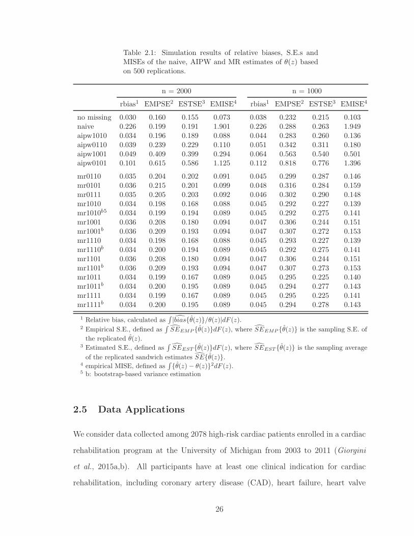
Table 2.1: Simulation results of relative biases, S.E.s andMISEs of the naive, AIPW and MR estimates of θ(z) basedon 500 replications.
n = 2000 n = 1000
rbias1 EMPSE2 ESTSE3 EMISE4 rbias1 EMPSE2 ESTSE3 EMISE4
no missing 0.030 0.160 0.155 0.073 0.038 0.232 0.215 0.103naive 0.226 0.199 0.191 1.901 0.226 0.288 0.263 1.949aipw1010 0.034 0.196 0.189 0.088 0.044 0.283 0.260 0.136aipw0110 0.039 0.239 0.229 0.110 0.051 0.342 0.311 0.180aipw1001 0.049 0.409 0.399 0.294 0.064 0.563 0.540 0.501aipw0101 0.101 0.615 0.586 1.125 0.112 0.818 0.776 1.396
mr0110 0.035 0.204 0.202 0.091 0.045 0.299 0.287 0.146mr0101 0.036 0.215 0.201 0.099 0.048 0.316 0.284 0.159mr0111 0.035 0.205 0.203 0.092 0.046 0.302 0.290 0.148mr1010 0.034 0.198 0.168 0.088 0.045 0.292 0.227 0.139mr1010b5 0.034 0.199 0.194 0.089 0.045 0.292 0.275 0.141mr1001 0.036 0.208 0.180 0.094 0.047 0.306 0.244 0.151mr1001b 0.036 0.209 0.193 0.094 0.047 0.307 0.272 0.153mr1110 0.034 0.198 0.168 0.088 0.045 0.293 0.227 0.139mr1110b 0.034 0.200 0.194 0.089 0.045 0.292 0.275 0.141mr1101 0.036 0.208 0.180 0.094 0.047 0.306 0.244 0.151mr1101b 0.036 0.209 0.193 0.094 0.047 0.307 0.273 0.153mr1011 0.034 0.199 0.167 0.089 0.045 0.295 0.225 0.140mr1011b 0.034 0.200 0.195 0.089 0.045 0.294 0.277 0.143mr1111 0.034 0.199 0.167 0.089 0.045 0.295 0.225 0.141mr1111b 0.034 0.200 0.195 0.089 0.045 0.294 0.278 0.143
1 Relative bias, calculated as∫|biasθ(z)/θ(z)|dF (z).
2 Empirical S.E., defined as∫SEEMP θ(z)dF (z), where SEEMP θ(z) is the sampling S.E. of
the replicated θ(z).3 Estimated S.E., defined as
∫SEEST θ(z)dF (z), where SEEST θ(z) is the sampling average
of the replicated sandwich estimates SEθ(z).4 empirical MISE, defined as
∫θ(z)− θ(z)2dF (z).
5 b: bootstrap-based variance estimation
2.5 Data Applications
We consider data collected among 2078 high-risk cardiac patients enrolled in a cardiac
rehabilitation program at the University of Michigan from 2003 to 2011 (Giorgini
et al., 2015a,b). All participants have at least one clinical indication for cardiac
rehabilitation, including coronary artery disease (CAD), heart failure, heart valve
26

repair or replacement, as well as heart transplantation. Our main interest in this
application is to evaluate the effect of ozone exposure two days prior to the resting
seated systolic blood pressure (SBP). We consider a subset of 704 subjects with
measured ozone exposure, of which 308 (44%) have missing SBP because of failure
to appear at the evaluation exam. For this study cohort, subjects are between 20
and 86 years old, 73% are male and 31% are current or former smokers. The ozone
exposure data are collected two days prior to the exam date from an air pollutants
monitoring site maintained by the Michigan Department of Environmental Quality to
allow for investigation on the delayed effect on the BP outcomes after ozone exposure.
The ozone exposure among our study cohort ranges from 13.1 to 75.5 ppb, with a
median 36.5 ppb and interquartile-range (31.5, 41.8). Although the ozone exposure
has been reported to be significantly associated with increased blood pressure (Day
et al., 2017), the functional form of such an association remains unclear, and is known
as non-linear scientifically.
We apply the MRKEEs method to investigate such a potentially non-linear relation-
ship. Since this is an observational study with missing data and thus we are not
sure of the missingness mechanism, we fit two generalized linear regression models,
using logit link and probit link separately, both with ozone level, age, gender, BMI
and smoking status as the potential predictors. We also include quadratic terms of
BMI and age, as suggested by previous literature (Hirano et al., 2003; Wooldridge,
2007), where they found that overparameterization of missingness probability leads
to a more precisely determined point estimate. We use linear regression to fit two
conditional mean models with different specifications: one with quadratic age and
BMI terms and one without, along with other covariates. Model diagnosis detects
no significant deficiencies in fitting all these four models. Thus we applied MRKEEs
with these four working models together. We also fit naive KEEs to the data for
comparison and use EBBS for bandwidth selection for both methods. The variances
27

are estimated using bootstrap for MRKEE and sandwich estimator for naive KEEs,
respectively. The estimated curves and their 95% CIs are shown in Figure 2. Here
we focus our discussion mainly on subjects with ozone exposure from 20 to 50 ppb,
because there are very few patients and kernel estimates are unstable outside this
range. From Figure 2, the multiply robust kernel regression curve shows that in-
creasing ozone exposure is associated with higher SBP, consistent with findings in the
literature (Day et al., 2017). Such an interesting relationship tends to reach a flato
as the ozone level reaches high, which makes sense because the SBP cannot explode
after reaching high enough. In contrast, the naive complete-case analysis suggests
that SBP is relatively stable (around 115 mmHg) and may even slightly decrease as
the ozone exposure increases. Notice that among this study cohort, older participants
have a higher chance to be absent from the exam, but in the meanwhile, they could
be more susceptible to ozone in terms of blood pressure. Therefore, the naive KEEs
estimator using only complete cases fails to capture the increasing trend and thus
leads to a biased estimate. In contrast, our MRKEEs analysis accounts for the bias
due to missing data and suggests that SBP increases relatively fast when subjects
start getting exposed to ozone, with the SBP increase slows down as ozone exposure
keeps increasing after a certain level.
2.6 Discussion
In this chapter, we proposed a novel multiply robust kernel estimating equations
(MRKEEs) method for local polynomial regression when the outcome is missing at
random. This method incorporates the auxiliary information by utilizing weights
computed through the empirical likelihood method based on multiple working models
for the selection probability and/or the outcome regression. Compared to the doubly
robust AIPW kernel estimation, the proposed MRKEEs method provides more pro-
tection against model misspecification, and the resulting estimator is consistent when
28

|||| | || || | || | || | ||| || |||| || | || || || | ||| || ||| || ||| | ||| || | |||| || ||| || ||| || || || || | || ||| | ||| | || ||||| | ||| || ||| ||| || || ||| ||| ||| || ||| || || | ||| | ||| || | || ||| | ||| || |||| | ||| | ||| | || | || || ||| || || || || || |||||| | ||| || | || || ||| || | || ||||| || ||| | || ||| ||||| |||| | || | ||| ||| ||| || || ||||||||| |||||| || |||| | |||| | || | |||||| ||| || | || || ||| | || | | |||| | |||| || ||| | | |||| || ||| | | | ||| |||| || || ||| ||| || ||| || | || | |||||| ||| || || |||| | || || || |||| || | || || |90
100
110
120
130
20 30 40 50 60O3 Exposure 2 Days Prior to Exam (ppb)
SB
P (m
mH
g)
Multiply Robust
Naive
Figure 2.3: The naive and multiply robust KEE estimates of ozone exposure (in ppb)on systolic blood pressure. Each vertical tick mark along the x-axis standsfor one observation.
any one of those working models is correctly specified. Moreover, when correct models
are used for both quantities, this MRKEE estimator achieves the optimal efficiency
that the optimal AIPW estimator can achieve. Simulation studies indicate that the
proposed estimator generally has better finite sample performance in terms of both
bias and efficiency. Although there is no theory regarding the bias when neither class
contains a correct model, under MAR we are able to investigate the working models
for Pr(R = 1|Z,U) and E(Y |Z,U) using observed data. Regular model checking and
diagnostics are useful in practice, and we will gain efficiency when any one of the
working models for E(Y |Z,U) is approximately correct.
As pointed out in Han and Wang (2013) and Han (2014b), the weight calculation
may encounter numerical issues when the sample size is small, or the number of
constraints is large. This might happen more often for kernel regression due to the
29

locality. Therefore some caution is needed when applying this method to datasets
with extremely small sample sizes.
The proposed method can be generalized to cases with multiple covariates. One
possible extension would be modifying the proposed methods to generalized partially
linear model
E(Y |X, Z) = µ(XTβ + θ (Z)
)
where X denotes a covariate vector, β is the parameter vector and θ is an unknown
smooth function. When Y is missing at random, β and θ(z) can be estimated in
an iterative fashion based on MRKEEs and a multiply robust version of the profile
estimating equations for β.
Another possible extension would be on single index models assuming that the con-
ditional mean depends on X and Z through a linear combination XTβX + ZβZ ;
i.e.
E(Y |X, Z) = µθ(XTβX + ZβZ
),
where θ (·) is an unknown smooth function that we wish to estimate. Parameters
β = (βX , βZ) and θ(·) can be estimated using a similar iterative method. These
extensions will be reported elsewhere.
30
CHAPTER III
Stochastic Tree Search for Estimating Optimal
Dynamic Treatment Regimes
3.1 Introduction
The emerging field of precision medicine has gained prominence in the scientific com-
munity. It aims to improve healthcare quality through tailoring treatment by consid-
ering patient heterogeneity. One way to formalize precision health care is dynamic
treatment regimes (DTRs, e.g. Murphy , 2003; Robins , 2004), which are sequential
decision rules, one per stage, mapping patient-specific information to a recommended
treatment. Consequently, DTRs provide health care that is individualized and also
adapted over time to changes in patient status. This is especially valuable in chronic
health management (e.g. Zhao et al., 2015). Typically, we define optimal DTRs as
the ones that maximize each individual’s long term clinical outcome when applied to
a population of interest, and thus identification of optimal DTRs becomes the key to
precision health care.
Various methods for estimating optimal DTRs have been proposed; some examples
include marginal structural models (e.g. Murphy et al., 2001; Wang et al., 2012),
G-estimation of structural nested mean models (e.g. Robins , 2004), likelihood-based
31

approaches (e.g. Thall et al., 2007), Q-learning (e.g. Nahum-Shani et al., 2012), A-
learning (e.g. Murphy , 2003; Schulte et al., 2014), outcome weighted learning (OWL,
Zhao et al., 2012, 2015), and other classification or supervised learning methods (e.g.
Zhang et al., 2012, 2013). Most of these methods require specifying working mod-
els for the treatment assignment mechanism, or the conditional outcome, or both,
which can be difficult when limited knowledge of observed data is available. Besides,
the working model specification can be especially challenging in the presence of a
moderate-to-large number of covariates. Qian and Murphy (2011), Zhao et al. (2011)
and Moodie et al. (2014) developed various nonparametric Q-learning methods, and
Murray et al. (2018) developed a Bayesian machine learning approach based on non-
parametric Bayesian regression models. Such data-driven methods are flexible and
mitigate the risk of model misspecification; however, the resulting DTRs are difficult
to interpret and thus obstruct human experts from understanding the regimes. There-
fore, it is often desirable to have interpretable and parsimonious DTRs, as they bridge
the gap between clinician’s domain expertise and data-driven treatment strategies.
The tension between model interpretability and prediction accuracy occurs because of
competing objectives: interpretability favors simple and generalizable models, while
accuracy often means specialization and sophistication.
In response, a recent research stream has focused on rule-based learning methods
for estimating interpretable optimal treatment regimes. Zhang et al. (2015, 2018b)
proposed a list-based approach to estimate optimal DTRs as a sequence of if-then
clauses. This method is flexible since nonparametric kernel ridge regression is used
for regime value modeling, but one drawback is that such list-based methods are
computationally demanding and therefore, each clause only thresholds two covariates.
As an alternative, Laber and Zhao (2015) and Tao et al. (2018) proposed tree-based
methods through sequentially maximizing the improvement in purity measures for the
quality of the regimes. However, these semiparametric methods will perform poorly
32

when working models do not have a good approximation of the underlying truth,
which is likely the case with fairly complex data.
To overcome these limitations, we propose a stochastic tree-based reinforcement learn-
ing method, ST-RL, which combines the powerful predictive model with an inter-
pretable decision tree structure, for estimation of optimal DTRs in a multi-treatment,
multi-stage setting. At each stage, ST-RL evaluates the regime quality using non-
parametric Bayesian additive regression trees, and then stochastically constructs an
optimal regime using a Markov Chain Monte Carlo (MCMC) tree search algorithm.
Our proposed ST-RL has stable performance even when the outcome of interest is
complicated by nonlinearity and low-order interactions. ST-RL significantly reduces
the guesswork to specify working models, which makes it desirable, especially when
data come from complex observational studies. Moreover, compared to existing non-
parametric Q-learning methods, ST-RL constructs tree-structured DTRs that are
easy to interpret and visualize, which allows clinicians to verify, validate and refine
the treatment recommendations using their domain expertise. The greedy splitting
in all existing tree-based methods is likely to result in locally optimal or overly com-
plicated trees (Murthy and Salzberg , 1995; Duda et al., 2012). In contrast, ST-RL
improves the optimality and model parsimony by taking advantage of stochastic tree
search.
The rest of this chapter is organized as follows. Section 3.2 formalizes the problem of
estimating optimal DTRs and describes the proposed method along with the compu-
tational algorithm. Theoretical results are presented in Section 3.3. Sections 3.4 and
3.5 present the numerical studies and an application example, respectively, followed
by Section 3.6 that concludes with some discussion.
33

3.2 Stochastic Tree-based Reinforcement Learning
3.2.1 Dynamic Treatment Regimes
Suppose our data consist of n i.i.d. trajectories (Xt, At, Rt)Tt=1 that come from
either a randomized trial or an observational study, where t ∈ 1, 2, · · · , T denotes
the tth stage, Xt denotes the vector of patient characteristics accumulated during the
treatment period t, At denotes a multi-categorical or ordinal treatment indicator with
observed value at ∈ At = 1, . . . , Kt, Kt (Kt ≥ 2) is the number of treatment options
at the tth stage, and Rt denotes the immediate reward following At. We further let
Ht denote patient history before At, i.e. Ht = (Xi, Ai, Ri)t−1i=1,Xt. We consider
the overall outcome of interest as Y = f(R1, . . . , RT ), where f(·) is a prespecified
function (e.g., sum, last value, etc.), and we assume that Y is bounded, with higher
values of Y preferable.
We denote a DTR, a sequence of individualized treatment rules, as g = (g1, . . . , gT ),
where gt maps from the domain of patient history Ht to the domain of treatment
assignment At. To define the optimal DTRs, we use the counterfactual outcome
framework of causal inference and start from the last stage in a reverse sequential
order. At the final stage T , let Y ∗(A1, . . . , AT−1, aT ), or Y∗(aT ) for brevity, denote
the counterfactual outcome had a patient been treated with aT conditional on previous
treatments (A1, . . . , AT−1), and define Y ∗(gT ) as the counterfactual outcome under
regime gT , i.e.,
Y ∗(gT ) =KT∑
aT=1
Y ∗(aT )IgT (HT ) = aT.
The performance of gT is measured by its value function V (gT ) (Qian and Mur-
phy , 2011), which is defined as the mean counterfactual outcome had all patients
followed gT , i.e. V (gT ) ≡ EY ∗(gT ). Therefore, the optimal regime goptT satisfies
V (goptT ) ≥ V (gT ) for all gT ∈ GT , where GT denotes the set of regimes of interest. In
34

order to identify optimal DTRs using observed data, we make the standard assump-
tions to link the distribution law of counterfactual data with that of observational data
(Murphy et al., 2001; Robins and Hernan, 2009). First we assume consistency, i.e.
the observed outcome is the same as the counterfactual outcome under the treatment
actually assigned, i.e. Y =∑KT
aT=1 Y∗(aT )I(AT = aT ), which also implies that there is
no interference between subjects. We also assume Y ∗(1), . . . , Y ∗(KT ) |= AT | HT ,
where |= denotes statistical independence, i.e. no unmeasured confounding assump-
tion (NUCA). Finally, we assume Pr(AT = aT |HT ) ∈ (c0, c1) is bounded by c0 and
c1, where 0 < c0 < c1 < 1. Under these assumptions, the optimal regime at stage T
can be written as
goptT = argmaxgT∈GT
E
[KT∑
aT=1
E(Y |AT = aT ,HT )IgT (HT ) = aT ],
where the outer expectation is taken with respect to the joint distribution of the
observed data HT .
At an intermediate stage t (1 ≤ t ≤ T−1), we consider Y ∗(A1, . . . , At−1, gt, goptt+1, . . . , g
optT ),
a conditional counterfactual outcome under optimal regimes for all future stages, had
a patient following gt at stage t (Murphy , 2005; Moodie et al., 2012). Similarly un-
der the three aforementioned assumptions, the optimal regime goptt at stage t can be
defined as
goptt = argmaxgt∈Gt
EY ∗(A1, . . . , At−1, gt, g
optt+1, . . . , g
optT )
= argmaxgt∈Gt
E
[Kt∑
at=1
E(Yt|At = at,Ht)Igt(Ht) = at],
where Gt is the set of all potential regimes at stage t, YT = Y at stage T , and at any
35

earlier stage t, Yt can be defined recursively using Bellman’s optimality:
Yt = E
Yt+1|At+1 = goptt+1(Ht+1),Ht+1
, t = 1, · · · , T − 1,
i.e. the expected outcome assuming optimal regimes are followed at all future stages.
3.2.2 Bayesian Additive Regression Trees
Accurate estimation of value function is the key to estimating optimal DTRs. To
mitigate the risk of model misspecification, multiple nonparametric regression meth-
ods have been introduced in estimating optimal DTRs, and some recent literature
advocates the use of Bayesian nonparametric approaches for causal inference (Hill ,
2011; Murray et al., 2018). Specifically, Bayesian additive regression trees (BART)
has become popular because it requires minimal effort for model specification and can
well approximate complex functions involving nonlinearity and interactions. Recent
developments in BART have provided theoretical support for its superior performance
(Rockova and van der Pas , 2017; Rockova and Saha, 2018). Moreover, modifications
of BART have been proposed to adapt to sparsity and various level of smoothness
(Linero, 2018; Linero and Yang , 2018), which further increase its potential in a wide
range of scenarios.
We use BART to fit the conditional outcome regression model E(Yt|At = at,Ht)
and then predict the counterfactual outcomes for each subject. Other nonparametric
regression models can also be used. Specifically, we model the pseudo-outcome at an
arbitrary stage t using an ensemble of regression trees:
Yt =m∑
i=1
fi(Ht, At;Mi) + ǫ,
where ǫ ∼ N(0, 1), each of fi’s is a binary tree andMi is the parameter set charac-
36

terizing the i-th tree. The number of trees, m, is a tuning parameter which can be
selected using cross-validation. BART combines a large number of weak decision tree
learners into a strong one to approximate complex functions, and uses a regularization
prior for each tree to penalize overly complex trees and hence prevent overfitting. We
use the average of after burn-in samples, which approximates the posterior mean, to
obtain a prediction E(Yt|At,Ht). For technical details readers are refered to Chipman
et al. (2010). As a result, the optimal regime at stage t, goptt can be estimated as
goptt = argmaxgt∈Gt
Pn
[Kt∑
at=1
E(Yt|At = at,Ht)Igt(Ht) = at]. (3.1)
3.2.3 Stochastic Tree Search Algorithm
Constructing an optimal binary decision tree is known to be NP-complete (Laurent
and Rivest , 1976); an exhaustive search is infeasible with even a fairly small number
of nodes. Existing tree-based methods iteratively maximize the improvement in a
purity function at each splitting. Although such greedy algorithms often work rea-
sonably well, they may be affected by local optimality. As a result, the estimated
sub-optimal, unnecessarily complex tree-structured DTRs may have compromised
quality and interpretability. Consider a toy example with two baseline variables, X1
and X2, both uniformly distributed on the interval [0,1], and a randomly assigned
binary treatment A = 0 or 1. The underlying optimal regime gopt(X1, X2) = 1 when
(X1 > 0.5, X2 > 0.5), or (X1 < 0.5, X2 < 0.5), and otherwise gopt(X1, X2) = 0. We
assume a linear reward function Y = X1 + X2 + βIA = gopt(X1, X2) + ǫ, where
ǫ ∼ N(0, 1). It is obvious that no matter how we partition the feature space using a
tree-based method to assign treatments at the first step, in principle each treatment
group always has half of patients ending up with suboptimal treatments. Therefore,
the target purity remains the same regardless of any partition in this case, and thus
the existing tree-based methods (e.g. Laber and Zhao, 2015) will fail to identify the
37

true optimal regime.
To balance exploration and exploitation, we propose to stochastically search the tree
space for the optimal regime using a Markov chain Monte Carlo (MCMC) algorithm
(Chipman et al., 1998; Denison et al., 1998; Wu et al., 2007). To make the pre-
sentation clear in this section, we suppress the stage subscript t, but the following
procedure works for any stage t. Denote a tree-based regime as g = (P,R), where P
is the parameter set which characterizes the tree topology – i.e., splitting variables,
splitting threshold, and the topological arrangement of nodes and edges – and R is
the treatment assignment rule for each leaf node. Note for any given P, R can be de-
termined by R = argmaxR∈R V (g), i.e., the treatment assignment at each leaf which
maximizes the expected regime value. Given the observed data, we sample P from
π(P|A,H) ∝ π(P)f(A|P,H), (3.2)
where A denotes the observed treatment at the current stage and H denotes pa-
tient medical history up to the current stage. However, this sampling procedure is
inefficient especially when a large proportion of patients did not receive their opti-
mal treatments, in which case the regular stochastic search might fail to converge to
the optimal regime. Alternatively, we use π(P|Aopt,H) to approximate (3.2), where
Aopt = argmaxa∈(1,···,K) E(Y |A = a,H) is the estimated optimal treatment and can
be viewed as a warm start.
We specify π(P) using a tree growing process. Let P = (T ,ρ,η), where T is the
topological arrangement of nodes and edges (i.e. a tree skeleton), ρ denotes the
splitting variables, and η denotes the corresponding splitting thresholds. Then the
prior distribution over P can be decomposed as
π(P) = π(T )π(ρ|T )π(η|T ,ρ). (3.3)
38

Throughout this process, we set π(ρ|T ) and π(η|T ,ρ) to be uniform, i.e. given the
tree structure, each variable is equally likely to be selected for splitting, and splitting
can take place uniformly on the domain of selected splitting variable. The distribution
π(T ) is specified using a tree growing process. We first draw the tree size s(T ) from
a shifted Poisson distribution Pois(λ)+1, with the shift used to avoid an empty tree.
Growing a tree with a given size s(T ) can be viewed as cascading down s(T ) leaf
nodes from the root. Assuming that at each internal node the available leaf nodes
independently pick the left or right subtree with equal probability, π(T ) can be written
as πPoisλ s(T )−1∏u∈T β(sul|su), where πPois
λ denotes the probability mass function of
a Poisson random variable with mean λ, u denotes any internal node, su is the number
of available leaf nodes at u, and sul is the number of leaf nodes picking the left subtree
of u. We set β(sul|su) to be uniform β(sul|su) = 1/(su − 1), for sul = 1, · · · , su − 1.
Such specification of π(T ) favors balanced trees, meaning that for a given size, the
algorithm penalizes deep trees by assigning them smaller probabilities. For more
details regarding the prior specification, the readers are referred to Wu et al. (2007).
Note that the use of uniform distributions assumes no domain knowledge available a
priori; however, other distributions could be used to incorporate human expertise. In
practice, the choice of Poisson parameter should reflect preferences over the regime
complexity, especially when data are limited.
To obtain f(Aopt|P,H), we assume that multi-level Aopt within each leaf node follows
i.i.d. multinomial distributions (binomial in case of two-level treatment), leaf node
parameters follow Dirichlet distributions, and leaf nodes are independent. Conse-
quently,
f(Aopt|P,H) ∝∫
Θ
f(Aopt|P,H,Θ)π(Θ|P)dΘ
can be calculated analytically because of Dirichlet-Multinomial conjugacy. Thus leaf
parameters Θ are not involved in the sampling scheme.
39

Algorithm 1: MCMC Algorithm
Result: gopt = (goptt )Tt=1
Initialize P(0) ∼ π(P);
for i← 1, 2, · · · do1. Propose P∗ using one of the proposals q(P∗|P(i−1)): Grow/Prune, Change,
Swap, Restructure;
2. Acceptance probability: α(P∗|P(i−1)) = min1, q(P(i−1)|P∗)π(P∗|Aopt,H)
q(P∗|P(i−1))π(P(i−1) |Aopt,H);
3. Sample u ∼ Uniform(0,1):
if u < α then
Set P(i) = P∗;
else
Set P(i) = P(i−1);
end
end
To implement the MCMC algorithm, we use multiple proposals, including grow/prune,
change and swap (Chipman et al., 1998; Denison et al., 1998). More specifically, the
grow/prune proposal either splits a randomly chosen leaf node or merges two sibling
leaves into one leaf node, with equal probabilities. The change proposal randomly se-
lects an internal node and resamples the splitting rule using π(ρ|T ) and π(η|T ,ρ). In
addition to these two local movements, swap proposal is more aggressive: it randomly
picks a node Np and one of its children Nc, both of which are internal nodes, and
swaps their splitting rules, i.e., swaps both splitting variables and the corresponding
thresholds. As a result, the whole subtree originally rooted from Np will be restruc-
tured. To facilitate a broader stochastic search, we adopt restructure proposal as in
Wu et al. (2007): for any given tree, the restructure proposal attempts to construct
a different tree while maintaining the current partitioning, i.e., searching for a new
tree with the same leaf nodes. This radical proposal drastically modifies the structure
40

of a tree while preserving the information accumulated so far, which allows escaping
from local optimum and leads to a more efficient search on the tree space. Each
proposal has an associated probability; in our MCMC implementation, we assign the
grow/prune proposal with a probability of 0.5, the change proposal with a probability
of 0.5, the swap proposal with a probability of 0.2 and the restructure proposal with
a probability of 0.05. The algorithm is summarized as in Algorithm 1.
As mentioned above, for each sampled tree, the treatment assignment rule in each
leaf node R can be uniquely determined and the tree can be evaluated using V (g).
Therefore, the MCMC algorithm provides a powerful tool for stochastic regime con-
struction.
3.2.4 Implementation of ST-RL
ST-RL is implemented in a reverse sequential order. At the final stage T , the pseudo
outcome YT = Y , and therefore it can be directly used in regime estimation. At each
intermediate stage t < T , the pseudo outcome Yt relies on the optimal treatment
regimes in all future stages and needs to be estimated. To prevent bias accumulation,
we estimate Yt using the actual observed outcomes at stage t plus the predicted future
loss due to sub-optimal treatments (Huang et al., 2015); that is
ˆY t = Y +
T∑
j=t+1
E[ ˆY j|goptj (Hj),Hj]− E[ˆY j|Aj = aj ,Hj],
whereˆY T = Y and the conditional means are estimated using BART. The perfor-
mance of BART can be tuned by some hyperparameters, such as number of trees,
prior hyperparameters for node parameters and noise. These tuning parameters
can be selected using cross-validation; however, in simulation studies, we find that
the default parameters from Chipman et al. (2010) work well in practice. The al-
gorithm of ST-RL is outlined in Algorithm 2, where the value is estimated using
41

V (gt) = Pn[∑Kt
at=1 E(ˆY t|At = at,Ht)Igt(Ht) = at], and the conditional mean is
also estimated using BART.
Algorithm 2: ST-RL Algorithm
Result: gopt = (goptt )Tt=1
Initialize YT = Y ;
for t← T to 1 do
1. Estimate E(ˆY t|At = at,Ht) =
∑mi=1 fi(Ht, At;Mi) using BART for each
subject, where at = 1, · · · , Kt;
2. For each subject, obtain Aoptt = argmaxat∈(1,···,Kt) E(
ˆY t|At = at,Ht);
3. Perform a stochastic tree search using MCMC Algorithm 1;
4. Estimate the optimal regime using goptt = argmaxgt∈GtV (gt);
5. if t > 1 then
SetˆY t−1 =
ˆY t + E[
ˆY t|goptt (Ht),Ht]− E[
ˆY t|At = at,Ht];
else
Stop;
end
end
3.3 Theoretical Results
In this section we show that the estimated DTRs using ST-RL are well generalizable
on new data. We use . and & to denote inequality up to a constant, ||·||∞ and ||·||n to
denote the sup norm and empirical norm, respectively. At stage t ∈ (1, · · · , T ), there
are Kt treatment options a1, · · · , aKt, and we assume Kt is finite. An arbitrary tree-
structured treatment regime gt (with s leaf nodes) can be denoted as gt = (pt,At),
where pt denotes any partition of Ht with Kt subsets and At is a vector of the corre-
sponding treatment assignments. More specifically, pt = pit : pit ⊂ (L1, · · · , Ls)Kt
i=1
is coarser than L, and L = L1, · · · , Ls is the partition formed by leaf nodes of gt,
42

where the i-th leaf Li = ami < Htm < bmi, m = 1, · · · , dHt and dHt
is the number of
variables inHt. The partitioning subsets pit∩pjt = ∅ for any i 6= j, and⋃Kt
i=1 pit = Ht.
However, there is no natural ordering in a partition; to avoid ambiguity, we explic-
itly order partitioning subsets by defining variables and thresholds: suppose subset
pit contains two hyper-rectangular cells Li and Li′ , then it can be indexed by a
vector of lower bound in each dimension: I i = min(ami, ami′) : m = 1, · · · , dHt.
Two index vectors can be compared element-wise: there must exist some integer
m′ ∈ (1, · · · , dHt) such that I im′ < Ijm′ and I im′′ = Ijm′′ for ∀m′′ < m′ if i < j.
On the other hand, treatment assignment At represents the recommended treatment
sequence corresponding to the ordered subsets in any partition pt. Each subset has
a unique treatment recommendation, and Ait 6= Ajt for any i 6= j. We use σ(T )
to denote all tree-induced partitions with size Kt as described above. Similarly, we
denote the set of all possible treatment assignments as σ(A).
Remark. In reality, it might be the case that some treatment options do not associate
to any partitions, i.e., such treatments are sub-optimal for all patients. When this is
the case, we let the corresponding pi = ∅.
To facilitate the derivation, we need a distance metric between two partitions, d(p,p′).
Various metrics have been proposed: examples include Hamming distance, symmetric
difference and rank-based partition distance (Rossi , 2011). We use the minimum
sum of pair-wise symmetric difference of two partitions: d(pt,p′t) =
∑Kt
i=1 ρ(pit, pf(i)t),
where f(·) is a bijection from index set 1, · · · , Kt to itself, and ρ(pi, pj) = Pr(Ht ∈
pipj) = Pr(Ht ∈ pi∪pj \pi∩pj). It is easy to see d(pt,p′t) ≥ 0, d(pt,p
′t) = d(p′t,pt)
and it follows triangle inequality; moreover d(pt,p′t) = 0 does not imply pt = p′t.
Therefore d(pt,p′t) is a semi-metric.
Denote the conditional outcome regression model E(Yt|At,Ht) as Qt(At,Ht). For
43

each t, our proposed estimator can then be rewritten as
(pt, At) = argmaxpt∈σ(Tt),At∈σ(At)
Pn
[Kt∑
a=1
Qt(a,Ht)Kt∑
i=1
I(Ht ∈ pit)I(Ait = a)
]
= argmaxpt∈σ(Tt),At∈σ(At)
PnFt(pt,At),
where Ft(pt,At) denotes∑Kt
a=1 Qt(a,Ht)∑Kt
i=1 I(Ht ∈ pit)I(Ait = a), and Qt(a,Ht) =
E(ˆY t|At = a,Ht). Similarly, the optimal underlying tree-structured regime g∗opt is
defined as
(p∗t ,A∗t ) = argmax
pt∈σ(Tt),At∈σ(At)
EFt(pt,At). (3.4)
In addition to consistency, NUCA, and positivity assumptions, we also make the
following assumptions. First, we assume the variables are bounded. Note when the
dimension of Ht is fixed, the results presented later in this section are still valid, but
in that case, the following assumption of dHtcan be dropped.
Assumption 1. For each t, ||Ht||∞. log1/2 n, |Yt|. log1/2 n and dHt. log1/2 n.
Next we assume certain smoothness of Qt(at, ·) = E(Yt|At = at,Ht).
Assumption 2. For each t, Qt(at, ·) is α-Holder continuous, and 0 < α ≤ 1. That
is,
Qt(at, ·) : [0, 1]p → R; supHt1,Ht2∈[0,1]p
|Qt(at, Ht1)−Qt(at, Ht2)|||Ht1 −Ht2||α2
<∞,
where 0 < α ≤ 1. Moreover, ||Qt(at, ·)||∞. log1/2 n for all t.
To avoid overfitting, the class of trees under consideration cannot be too complex.
Lugosi et al. (1996) proved the consistency of a binary decision tree by restricting
the number of leaf nodes st to o(n/log n). Recently, Rockova and van der Pas (2017)
proved in regression case that the sampled tree size is bounded in probability when the
44

prior tree size is drawn from a Poisson distribution. These conditions are equivalent;
we have similar results for our proposed method, as shown in the following theorem.
Theorem 3.1 (Tree Complexity). For each t, if the stochastic tree search is as de-
scribed previously, then the sampled tree size, i.e., the number of leaf nodes st satisfies
Pr(st & ndHt/2α+dHt |Ht, A
optt )→ 0
in P n0 probability.
Theorem 3.1 guarantees that the tree size of our estimated optimal DTR using ST-
RL grows sub-linearly. In other words, ST-RL prevents from overfitting. Compared
to other existing tree-based methods, ST-RL does not require stopping rules and
pruning procedures, which are typically ad hoc. In addition, we make the following
assumption, which guarantees that the optimal tree-structured DTR exists and is
unique, i.e. any other optimal tree-structured DTRs (p∗′
,A∗′) will satisfy d(p∗′
,p∗) =
0 and A∗′ = A∗.
Assumption 3. For each t, the following inequalities hold:
• For all ǫ > 0, supd(p,p∗)≥ǫ EF (p,A∗) < EF (p∗,A∗); moreover, there exists a
constant κ > 0 such that EF (p,A∗)−EF (p∗,A∗) ≤ −κd2(p,p∗) as d(p,p∗)→
0.
• There exists a constant ǫ > 0 such that supA6=A∗ EF (p,A) < EF (p∗,A∗)− ǫ.
Given the above assumptions, the theorem below establishes the stage-specific finite
sample bound to evaluate the performance of goptt compared to goptt in terms of classi-
fication error and difference in value. For each t, we use Vt(gt) = E[∑Kt
at=1 E(Yt|At =
at,Ht)Igt(Ht) = at] to denote the stage-specific value function for an arbitrary
45

regime gt.
Theorem 3.2 (Finite Sample Bound). Under regularity conditions, for each t and
any ǫ > 0, we have
Pr(goptt 6= goptt ) . n−rt+ǫ,
PrVt(g
optt )− Vt(goptt ) & τn−rt+ǫ)
≤ e−τ ,
where rT = 23
αT
2αT+dHT
, and rt =23min( αt
2αt+dHt
, rt+1) for t < T .
Yang (1999) showed that the minimax convergence rate for nonparametric classifica-
tion in our case is O(nα/(2α+d)). The scaling factor 2/3 arises as a result of non-regular
argmax continuous mapping theorem (Kim et al., 1990; Kosorok , 2008) and implies
that interpretability is achieved at the cost of efficiency. At the final stage T , the
rate of convergence is determined by the convergence rate of the conditional outcome
regression estimator, which is shown to be O(n2α/(2α+d) log n) (Rockova and Saha,
2018). It becomes more complex at an earlier stage t since the rate of convergence at
stage t is also affected by convergence rates at later stages.
3.4 Simulation Study
We demonstrated the performance of ST-RL through a series of simulation studies,
including four single-stage scenarios and four two-stage scenarios. In each scenario
we generated training data with a sample size n = 500 and the dimension of baseline
variables p = 50, 100 and 200. The baseline covariates Xi, i = 1, · · · , p were generated
from a uniform distribution U(0, 1), with an AR1 correlation structure and a correla-
tion coefficient of 0.4. Following the same mechanism, we generate independent test
sets with a sample size of 1000.
46

We estimated the optimal regime using training data and then predicted the opti-
mal treatments for subjects in the test sets using our estimated optimal DTRs. The
following metrics were then calculated using test sets: opt% refers to the percent-
age of subjects correctly classified to their optimal treatments, EY ∗(gopt) refers
to the estimated counterfactual mean outcome under the estimated optimal regime
gopt. opt% measures the performance of the estimated optimal regime in assigning
future subjects to their optimal treatments, and EY ∗(gopt) measures the population
desirable outcome if following gopt. ST-RL was implemented using modified BART
with Dirichlet splitting rule prior to induce sparsity (Linero, 2018). Four methods
were compared with ST-RL: Q-learning with linear model (Q-Lin), nonparametric
Q-learning with random forest (Q-RF), outcome weighted learning implemented us-
ing CART (OWL-CART; Zhao et al., 2015) and tree-based reinforcement learning
(T-RL; Tao et al., 2018). In each scenario, the two metrics were averaged over 500
simulation replications.
3.4.1 Single-stage Scenarios
In single-stage setting, we considered four scenarios, all with three-level treatment
A taking values in 0, 1, 2. In scenarios I and II, the treatment A was gener-
ated from a multinomial distribution with probabilities π0, π1, π2, where π0 =
1/1 + exp(Xβ1) + exp(Xβ2), π1 = exp(Xβ1)/1 + exp(Xβ1) + exp(Xβ2) and
π2 = 1 − π0 − π1, where β1 = (−1,−1, 0, 2, 0,−1, 1,−1,−1, 2, 0, · · · , 0) and β2 =
(−1,−1,−1,−1, 2, 1, 1, 1, 1, 0, 0, · · · , 0). The underlying optimal treatment regime
gopt(H) was specified as:
gopt(H) =
0 X3 ≤ 0.35
1 X3 > 0.35, 2.5X22 − 0.5X1 ≤ 0.5
2 X3 > 0.35, 2.5X22 − 0.5X1 > 0.5
47

In scenario I, a simple reward function Y was used with equal loss on sub-optimal
treatments Y = 1−X4+X5−X1+X2+2∗I(gopt = A)+ǫ, and hereafter ǫ ∼ N(0, 1).
In contrast, scenario II used a simple reward but with different losses; i.e., the incurred
loss depended on the sub-optimal treatment received: Y = 1 + X4 + X5 + 2I(A =
0) 2 ∗ I(gopt = 0)− 1+ 1.5I(A = 2) 2 ∗ I(gopt = 2)− 1+ ǫ.
Scenarios III and IV generated treatment A from a rule-based treatment assignment
mechanism: A = I(X21 + X2
2 < 0.5) + I(X24 + X2
5 < 0.5), and a relatively com-
plex underlying optimal treatment regime: gopt(H) = I(2X24 + X2
4 > 0.6)[IX2 +
0.5 exp(X1)2 + X7 < 2.25 + IX2
3 − log(X5) − X6 < 3.5]. Moreover, scenarios
III and IV studied complicated reward functions. Scenario III used a reward with
equal loss due to sub-optimal treatments Y = 1 + 2X5 + 2 exp(X1) + 5Φ(X1)X22 +
5X3 log(X5 + 0.1) + exp2X2 + 1.5I(gopt = A) + ǫ, while scenario IV used a re-
ward with different losses Y = 1 + 2X5 + 2 exp(X1) + 5Φ(X1)X22 + 5X3 log(X5 +
0.1)+exp[2X2+2.5I(A = 0) 2 ∗ I(gopt = 0)− 1+2I(A = 1) 2 ∗ I(gopt = 1)− 1+
1.5I(A = 2) 2 ∗ I(gopt = 2)− 1] + ǫ, where Φ(·) stands for the cumulative distribu-
tion function of the standard normal distribution.
Table 3.1 summarizes the performance of the compared methods in all 4 scenarios. As
both T-RL and OWL-CART require estimation of the treatment assignment prob-
abilities, a multinomial logistic regression was fitted, with the observed treatment
as the dependent variable and all baseline covariates as explanatory variables. In
addition, T-RL requires specification of an outcome regression model for E(Y |X),
which we assumed to be a linear regression model. In all four scenarios, ST-RL
had outstanding performance compared to the other methods, even when there is
a moderately large number of variables (p=200) and a relatively small sample size
(n=500). The list-based method had competitive performance in Scenarios I and
II; however, its performance was compromised when the underlying optimal regime
48

Table 3.1: Simulation results for single-stage scenarios I-IV, with 50, 100, 200 baseline covariates and sample size 500. Theresults are averaged over 500 replications. opt% shows the median and IQR of the percentage of test subjectscorrectly classified to their optimal treatments. EY ∗(gopt) shows the empirical mean and the empirical standarddeviance of the expected counterfactual outcome under the estimated optimal regime.
Number of Scenario I Scenario II Scenario III Scenario IV
Baseline Covariates EY ∗(gopt) opt% EY ∗(gopt) opt% EY ∗(gopt) opt% EY ∗(gopt) opt%
50
Q-Lin 3.3 (0.1) 65.0 (4.5) 2.5 (0.1) 64.8 (5.2) 16.8 (0.4) 73.5 (3.9) 26.7 (0.9) 73.4 (4.1)
Q-RF 3.8 (0.1) 89.9 (7.0) 2.5 (0.2) 60.4 (17.2) 16.9 (0.5) 70.6 (5.5) 27.8 (1.0) 67.5 (4.1)
OWL 2.7 (0.1) 36.2 (5.8) 1.8 (0.2) 38.2 (6.9) 15.7 (0.4) 60.7 (4.3) 24.0 (1.2) 65.0 (5.7)
List 3.9 (0.1) 95.0 (3.0) 3.1 (0.1) 94.6 (3.3) 17.6 (0.5) 77.0 (5.2) 27.1 (1.1) 63.8 (6.5)
T-RL 3.7 (0.2) 88.0 (9.0) 2.9 (0.2) 83.2 (16.3) 17.7 (1.0) 85.6 (10.8) 28.0 (1.7) 70.6 (5.8)
ST-RL 3.9 (0.1) 95.4 (2.0) 3.2 (0.0) 95.8 (1.5) 18.2 (0.6) 90.4 (3.1) 29.9 (0.9) 89.4 (3.8)
100
Q-Lin 2.9 (0.1) 44.1 (6.3) 2.0 (0.2) 44.6 (6.8) 14.6 (0.9) 56.5 (8.5) 21.8 (2.2) 57.5 (9.2)
Q-RF 3.7 (0.2) 89.2 (9.2) 2.4 (0.2) 54.0 (19.2) 16.7 (0.5) 68.8 (5.4) 27.6 (1.0) 66.5 (4.4)
OWL 2.7 (0.1) 34.4 (3.1) 1.7 (0.1) 35.2 (4.4) 15.9 (0.4) 63.1 (4.4) 24.6 (1.1) 67.1 (5.1)
List 3.9 (0.1) 95.3 (2.7) 3.1 (0.1) 94.8 (3.3) 17.5 (0.5) 76.2 (5.6) 26.9 (1.1) 62.4 (5.9)
T-RL 3.0 (0.4) 52.4 (31.5) 2.2 (0.4) 50.9 (31.1) 16.4 (2.0) 76.0 (23.0) 25.2 (4.5) 65.0 (12.0)
ST-RL 3.9 (0.1) 95.2 (2.5) 3.1 (0.0) 95.8 (1.5) 18.0 (0.8) 90.0 (3.3) 29.7 (1.2) 89.2 (3.7)
200
Q-Lin 2.7 (0.1) 34.6 (4.3) 1.7 (0.1) 35.1 (4.4) 12.0 (0.7) 33.5 (6.9) 14.7 (1.9) 33.9 (6.8)
Q-RF 3.7 (0.2) 88.6 (9.5) 2.3 (0.2) 50.4 (20.7) 16.5 (0.5) 67.2 (5.4) 27.4 (1.2) 65.7 (4.5)
OWL 2.7 (0.1) 34.0 (2.5) 1.7 (0.1) 34.4 (2.7) 15.9 (0.4) 63.1 (3.7) 24.7 (1.1) 67.5 (5.0)
List 3.9 (0.1) 95.1 (3.4) 3.1 (0.1) 94.8 (3.3) 17.5 (0.5) 75.8 (5.7) 26.9 (1.1) 61.8 (5.3)
T-RL 2.7 (0.1) 33.5 (3.0) 1.7 (0.2) 33.4 (2.9) 12.7 (1.5) 35.8 (11.4) 15.9 (4.1) 35.6 (10.9)
ST-RL 3.8 (0.2) 94.8 (3.8) 3.1 (0.1) 95.7 (1.7) 17.7 (1.2) 89.3 (4.8) 29.1 (2.3) 88.6 (4.9)
49

and reward became complex (scenarios III and IV). T-RL performed well when the
data dimension is relatively low, even when both propensity and outcome regression
models were incorrectly specified. When the number of variables increased, T-RL
performed poorly. Q-Learning methods also significantly varied by case. Both Q-Lin
and Q-RF performed better with fewer noise variables, with Q-RF being more sta-
ble against increased dimensionality. Consistent with the simulation findings in Tao
et al. (2018), OWL-CART had an unsatisfactory performance, which is probably due
to both misspecification of propensity score models and a low percentage of subjects
receiving optimal treatments in the simulated trial or observational data.
3.4.2 Two-stage Scenarios
We considered four two-stage scenarios with a three-level treatment at each stage,
and the outcome was defined as the sum of immediate rewards from each stage,
i.e. Y = R1 + R2. In scenarios V and VI, stage 1 treatment A1 was generated
from a multinomial distribution similar to Section 3.4.1, with parameters β11 =
(−1,−1, 0, 2, 0,−1, 1, 1,−1, 0, 0, · · · , 0) and β12 = (−1,−1,−1,−1, 0, 1, 0, 0, 1, 2, 0, · · · ,
0). In scenario V, the underlying optimal DTR had a tree structure gopt1, tree = I(X1 <
0.7) I(X5 < 0.7) + I(X10 > 0.3), while in scenario VI the optimal DTR did not
have a tree structure gopt1, nontree = I(X3 > 0.35)I(2.5X22 − 0.5X1 > 0.5) + 1. In both
scenarios V and VI, the immediate reward R1 was generated from Y = 1 + X2 +
X4 +X6 + 2I(A = 0) 2 ∗ I(gopt = 0)− 1 + 1I(A = 1) 2I(gopt = 1)− 1 + 3I(A =
2) 2I(gopt = 2)− 1+ ǫ.
At stage 2, in both scenarios V and VI the treatment A2 = 0, 1, 2 was gener-
ated from a multinomial distribution with probabilities π20, π21, π22, where π20 =
1/1 + exp(Xβ21 + 0.2R1) + exp(Xβ22 + 0.2R1), π21 = exp(Xβ21 + 0.2R1)/1 +
exp(Xβ21 + 0.2R1) + exp(Xβ22 + 0.2R1) and π22 = 1 − π20 − π21, with β21 =
(−1,−1, 1, 2, 0,−1, 1, 0, 1,−2, 0, · · · , 0) and β22 = (1, 1,−1,−1,−2, 1, 1, 1, 0,−1, 0, · · · ,
50

0). Similarly to stage 1, scenario V used a tree-type optimal treatment regime
gopt2, tree = I(R1 > 1)I(X10 < 0.6) +1 and scenario VI used a non-tree-type regime
gopt2, non−tree = I(1.5X2 +X4 + 0.5R1) + I(0.5R1 +X1 +X9 > 2). The stage 2 reward
R2 was then generated from R2 = 1 +X1 + 2X5 + 2I(A2 = 0)2I(gopt2 = 0)− 1
+
1.5I(A2 = 2)2I(gopt2 = 2)− 1
+ ǫ.
We also evaluated the performance of our proposed ST-RL in a randomized trial set-
ting through scenarios VII and VIII. In both scenarios, 3-level treatments A1 and A2
were generated from a multinomial distribution with probabilities (13, 13, 13). Scenario
VII used simple tree-type regimes at both stages: gopt2, tree = I(X1 > 0.15)I(X2 > 0.25)
+ I(X2 > 0.6), and gopt2, tree = I(X3 > 0.2) I(R1 > 0) + I(X5 < 0.8). Scenario
VIII used non-tree-type underlying optimal regimes: gopt1, nontree = I(2X24 + X4 >
0.6)I(X2+0.5 exp(X1)2+X7 < 2.25)+ I(X2
3− log(X5)−X6 < 3.5) and gopt2, nontree =
I(1.5X2+X4+0.5R1 > 2)+ I(0.3R1+X1+X9 > 2.5). In both scenarios, a complex
and non-linear reward function was used for stages 1 and 2: R1 = exp2 + 0.5X4 −
|4.5X1− 1|(A1− gopt1 )2+ ǫ and R2 = exp1+X2− |1.5X3+X4+1|(A2− gopt2 )2+ ǫ.
Simulation results of two-stage treatment regimes are summarized in Table 3.2. Es-
sentially the comparison with other methods showed similar trends as observed in
one-stage scenarios. For OWL, we applied the backward OWL (BOWL) method in
Zhao et al. (2015). ST-RL had a reliable performance in both confounded (scenarios V
and VI) and randomized (scenarios VII and VIII) settings, even with a large amount
of noise interference. The performance of list-based method varied significantly by
simulation scenarios: when the underlying optimal regime was fairly complex (VI and
VIII), the constraint of at most two variables in each clause might be too restrictive
and thus list-based method did not work well. In addition, the list-based method did
not always perform consistently even in a simple setting (V). T-RL performed well in
randomized settings (VII and VIII), but was severely affected when working models
51
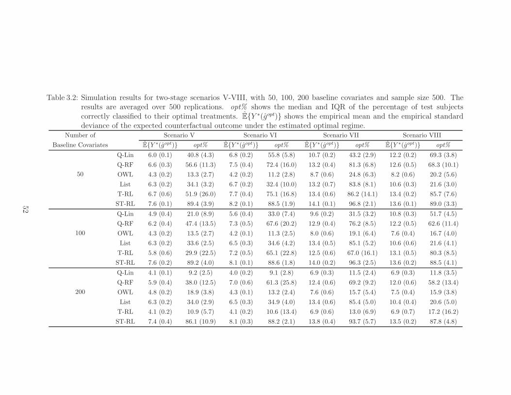
Table 3.2: Simulation results for two-stage scenarios V-VIII, with 50, 100, 200 baseline covariates and sample size 500. Theresults are averaged over 500 replications. opt% shows the median and IQR of the percentage of test subjectscorrectly classified to their optimal treatments. EY ∗(gopt) shows the empirical mean and the empirical standarddeviance of the expected counterfactual outcome under the estimated optimal regime.
Number of Scenario V Scenario VI Scenario VII Scenario VIII
Baseline Covariates EY ∗(gopt) opt% EY ∗(gopt) opt% EY ∗(gopt) opt% EY ∗(gopt) opt%
50
Q-Lin 6.0 (0.1) 40.8 (4.3) 6.8 (0.2) 55.8 (5.8) 10.7 (0.2) 43.2 (2.9) 12.2 (0.2) 69.3 (3.8)
Q-RF 6.6 (0.3) 56.6 (11.3) 7.5 (0.4) 72.4 (16.0) 13.2 (0.4) 81.3 (6.8) 12.6 (0.5) 68.3 (10.1)
OWL 4.3 (0.2) 13.3 (2.7) 4.2 (0.2) 11.2 (2.8) 8.7 (0.6) 24.8 (6.3) 8.2 (0.6) 20.2 (5.6)
List 6.3 (0.2) 34.1 (3.2) 6.7 (0.2) 32.4 (10.0) 13.2 (0.7) 83.8 (8.1) 10.6 (0.3) 21.6 (3.0)
T-RL 6.7 (0.6) 51.9 (26.0) 7.7 (0.4) 75.1 (16.8) 13.4 (0.6) 86.2 (14.1) 13.4 (0.2) 85.7 (7.6)
ST-RL 7.6 (0.1) 89.4 (3.9) 8.2 (0.1) 88.5 (1.9) 14.1 (0.1) 96.8 (2.1) 13.6 (0.1) 89.0 (3.3)
100
Q-Lin 4.9 (0.4) 21.0 (8.9) 5.6 (0.4) 33.0 (7.4) 9.6 (0.2) 31.5 (3.2) 10.8 (0.3) 51.7 (4.5)
Q-RF 6.2 (0.4) 47.4 (13.5) 7.3 (0.5) 67.6 (20.2) 12.9 (0.4) 76.2 (8.5) 12.2 (0.5) 62.6 (11.4)
OWL 4.3 (0.2) 13.5 (2.7) 4.2 (0.1) 11.3 (2.5) 8.0 (0.6) 19.1 (6.4) 7.6 (0.4) 16.7 (4.0)
List 6.3 (0.2) 33.6 (2.5) 6.5 (0.3) 34.6 (4.2) 13.4 (0.5) 85.1 (5.2) 10.6 (0.6) 21.6 (4.1)
T-RL 5.8 (0.6) 29.9 (22.5) 7.2 (0.5) 65.1 (22.8) 12.5 (0.6) 67.0 (16.1) 13.1 (0.5) 80.3 (8.5)
ST-RL 7.6 (0.2) 89.2 (4.0) 8.1 (0.1) 88.6 (1.8) 14.0 (0.2) 96.3 (2.5) 13.6 (0.2) 88.5 (4.1)
200
Q-Lin 4.1 (0.1) 9.2 (2.5) 4.0 (0.2) 9.1 (2.8) 6.9 (0.3) 11.5 (2.4) 6.9 (0.3) 11.8 (3.5)
Q-RF 5.9 (0.4) 38.0 (12.5) 7.0 (0.6) 61.3 (25.8) 12.4 (0.6) 69.2 (9.2) 12.0 (0.6) 58.2 (13.4)
OWL 4.8 (0.2) 18.9 (3.8) 4.3 (0.1) 13.2 (2.4) 7.6 (0.6) 15.7 (5.4) 7.5 (0.4) 15.9 (3.8)
List 6.3 (0.2) 34.0 (2.9) 6.5 (0.3) 34.9 (4.0) 13.4 (0.6) 85.4 (5.0) 10.4 (0.4) 20.6 (5.0)
T-RL 4.1 (0.2) 10.9 (5.7) 4.1 (0.2) 10.6 (13.4) 6.9 (0.6) 13.0 (6.9) 6.9 (0.7) 17.2 (16.2)
ST-RL 7.4 (0.4) 86.1 (10.9) 8.1 (0.3) 88.2 (2.1) 13.8 (0.4) 93.7 (5.7) 13.5 (0.2) 87.8 (4.8)
52

are wrong. Moreover, T-RL was more susceptible to noise interference.
3.5 Data Applications
We applied the proposed ST-RL to an esophageal cancer dataset of 1170 patients
collected at MD Anderson Cancer Center from 1998 to 2012. At baseline, patients
were between 20 to 91 years old, 85% male, 56% with advanced overall cancer stage
(stage III/IV), 19% with squamous cell carcinoma, 81% with Adenocarcinoma, and
44% with well/moderate tumor differentiation. Patients had an average tumor length
of 33mm with an interquartile range from 30mm to 37mm. A general treatment
strategy for optimizing long-term survival is neoadjuvant chemoradiation followed by
esophagectomy (surgery) (Nieman and Peters , 2013).
In this application, we primarily focused on the two-stage neoadjuvant chemoradiation
disease management before surgery. At baseline, patient characteristics were recorded
and denoted as X, which include patient information like age, gender, BMI, and
disease statuses such as ECOG performance, PET SUV, hypertension status, lesion
location, histology, differentiation, tumor length, and overall stage. At the initial
treatment stage, 41% patients received induction chemotherapy (ICT). We denote this
initial treatment as A1, with the value YES if treated with ICT and NO otherwise. An
intermediate measure of tumor response, R1, was recorded after this initial treatment
to evaluate the effect of A1, and R1 ranged from 0 to 5, with 0 being progression and
5 being the complete response.
At treatment stage 2, there were three radiation modalities: 39% of patients received
3D conformal radiotherapy (3DCRT), 45% patients received intensity-modulated ra-
diation therapy (IMRT) and 16% received proton therapy (PT). We denote the stage
2 treatment as A2, following which, the tumor response R2 (same scale as R1) and any
development of new lesion N2 (0 if developed new lesion and 1 if not) were evaluated.
53

Furthermore, side effects were also recorded, including nausea S2,1 (0 if experienced
nausea and 1 if not) and anorexia S2,2 (0 if experienced anorexia and 1 if not). We
defined a composite reward of interest Y = R1 +R2 +2N2 +2S2,1 +2S2,2 to measure
the effectiveness of this two-stage treatment regime. This composite reward balanced
multiple competing clinical priorities by incorporating tumor responses measured at
the end of two stages and accounting for new lesion development and side effects
along the treatment process. Missing data are imputed using IVEware (Raghunathan
et al., 2002).
We then applied ST-RL algorithm to the data described above. We used BART to
fit the response surface of E(Y2|A2 = a2,H2), where Y2 = Y , and obtain the optimal
tree-structured regime gopt2 . The same procedure was repeated for treatment stage
1 to obtain gopt1 , with H1 = X and Y1 = Y + E(Y2|gopt2 ,H2) − E(Y2|A2,H2). The
estimated optimal DTR was gopt = (gopt1 , gopt2 ), where
gopt1 =
YES if tumor differentiation = poor and cancer stage = I/II and
tumor length <41mm
NO otherwise
(3.5)
and
gopt2 =
PT if A1 = YES and tumor length > 29mm
IMRT if A1 = YES and tumor length < 29mm
3DCRT otherwise
(3.6)
The estimated optimal DTR suggests that at the initial treatment stage, ICT is
recommended for early-stage esophageal cancer patients with reasonably small-sized
tumors that are poorly differentiated. Although a randomized clinical trial (Ajani
et al., 2013) suggested that ICT before preoperative chemoradiation would not sig-
nificantly benefit the esophageal patient population in terms of complete pathologic
54

response and overall survival, our result can serve as a secondary analysis to help iden-
tify subgroups that might benefit from ICT in terms of immediate tumor response and
new lesion development. At treatment stage 2, our result showed that patients who
received ICT and had larger tumors should use PT while patients who received ICT
and had smaller tumors should use IMRT, all other patients should receive 3DCRT.
Although it is difficult to draw definitive conclusions regarding clinical outcomes from
the existing literature due to lack of published large trials comparing the three modal-
ities, clinical findings demonstrate that IMRT and PT allow the radiation beam to be
shaped more precisely to smaller tumors compared to 3DCRT (Xu and Lin, 2016).
This is consistent with our results that gopt2 suggests using PT/IMRT as an alterna-
tive treatment for patients if they already used ICT as their initial treatment, which
indicates they have a smaller, early-stage tumor according to gopt1 .
3.6 Discussion
The rapid developments in statistical machine learning have significantly enhanced
our ability to flexibly and accurately estimate the most appropriate treatment to
patients. However, explicit and interpretable decision rules are preferred by clini-
cians rather than a machine learning black-box. How to balance the accuracy gain
and compromise of interpretability has drawn attention. Efficient communication is
the key to any data-driven dynamic treatment regimes to make a practical impact.
Therefore, developing methodologies that are both theoretically sound and compu-
tationally efficient is critical for further promoting the broader impact of dynamic
treatment regimes (DTRs).
We have proposed a new method ST-RL to estimate optimal DTRs in multi-stage
multi-treatment settings using potentially large and complex observational data. ST-
RL combines flexible nonparametric BART estimation and stochastic policy search
55

to improve interpretability and quality of data-driven DTRs. Many existing methods
focus on randomized trial data; however, in practice, observational data is much
more common. Especially in large observational studies, often little is known about
the intervention assignment mechanism or the relationship between outcome and
covariates. In this case, our newly proposed data-driven and interpretable method ST-
RL can mitigate the model misspecification risk, and perform stably across different
scenarios. The estimated results are helpful to generate scientific hypotheses and to
provide insights on future biomedical research.
The proposed methods can be extended to other types of outcomes, such as binary and
right-censored survival data. One remaining question is how to improve the scalability
of the stochastic tree search when the data are sparse. With high-dimensional sparse
data, one can perform explicit variable selection before regime estimation; however,
how to ensure the selection consistency over multiple stages remains a challenge.
56

CHAPTER IV
A Flexible Tailoring Variable Screening Approach
for Estimating Optimal Dynamic Treatment
Regimes in Large Observational Studies
4.1 Introduction
Although the traditional “one-size-fits-all” medicine remains a common practice, it is
inadequate to provide optimal healthcare to each patient. In contrast, the emerging
personalized medicine considers population heterogeneity and is now widely recog-
nized as a promising approach for disease management and treatment for complex
health conditions. The idea of using precisely tailored therapies to accommodate
patient treatment response heterogeneity over time has been formalized as dynamic
treatment regimes (DTRs) in statistics (Murphy , 2003). DTRs are sequential decision
rules that individualize treatments while adapting to disease progression over time.
Optimal DTRs are mappings from up-to-date patient information to treatment rec-
ommendations at each stage, such that an average desirable long-term clinical reward
is maximized. Various methods have been proposed to estimate optimal DTRs, in-
cluding marginal structural models (Murphy et al., 2001), G-estimation of structural
nested mean models (Robins , 2004), likelihood-based approaches (Thall et al., 2007),
57

robust approaches (Zhang et al., 2012, 2013), machine learning methods (Zhao et al.,
2012, 2015; Laber and Zhao, 2015).
Nowadays, it is often the case that a large number of variables are collected in obser-
vational studies, which has brought new challenges in estimating optimal treatment
regimes. One popular example is the Omics data. More specifically, most exist-
ing methods require working model specification, such as the model of conditional
outcome regression, or the model of treatment assignment probability, or both. High-
dimensional data would increase the risk of model misspecification. Although non-
parametric techniques can potentially eradicate the need for working models, they are
known to be impacted by the curse of dimensionality. Furthermore, many existing
methods cannot even work without non-trivial modifications when p≫ n. Therefore,
it is of great interest to perform explicit variable selection before estimating optimal
DTRs when there is a large number of variables. Even though variable selection has
been extensively studied in the literature, it is understudied in the area of dynamic
treatment regimes. It was not until recently that this topic has drawn some attention.
In the pioneering work by Gunter et al. (2011), the authors proposed S-Score, a frame-
work for variable selection in treatment individualization. The authors reintroduced
the concept of prescriptive variables, i.e., variables having qualitative interactions
with treatment. Fan et al. (2016) extended this method to a multi-stage scenario and
proposed sequential advantage selection (SAS). SAS is closely related to Q-learning
and identifies prescriptive variables one at a time while taking into consideration the
variables that are already selected in previous steps. Another stream of research is
based on the framework of A-leaning. Lu et al. (2013) developed a penalized regres-
sion approach in single-stage setting; Shi et al. (2018) further proposed penalized
A-learning (PAL) in multi-stage scenario. In parallel, Zhang et al. (2018a) proposed
forward minimal misclassification error rate (ForMMER) selection from classification
perspective. Another line of research focuses on testing for qualitative interactions;
58

examples include Gail and Simon (1985); Chang et al. (2015); Hsu (2017); Shi et al.
(2019).
However, existing methods have some limitations. First of all, most existing meth-
ods, if not all, involve modeling the treatment effect contrast functions. As a result,
these methods are naturally restricted to treatments with two levels. Second, exist-
ing methods require working model specification. S-Score and SAS sequentially build
conditional outcome regression models; C-learning and PAL involve modeling the
contrasts using doubly robust estimator and therefore require modeling propensity
scores. For these methods, the quality of working models will determine the vari-
able selection performance; however, it is challenging to construct working models
in high-dimensional data. For example, SAS selects variables sequentially, therefore
will likely be biased when some confounding variables have not been included in the
model. Besides, ForMMER needs pre-screening procedure when constructing aug-
mented inverse probability weighted estimator (AIPWE) for contrasts when p > n.
Partially due to this reason, all existing methods are limited to randomized trial data.
In this chapter, we propose a variable selection procedure, sparse additive selection
(SpAS), to identify predictive and potential prescriptive variables in estimating opti-
mal DTRs. Our proposed method is closely related to Q-learning and is implemented
using backward induction. When modeling the Q-function, i.e., E(Y |X,A), we use
the nonparametric sparse additive model with strong heredity constraint: interactions
can only enter the model when both of its main effects are selected. This will help
improve model interpretability and plausibility. Such hierarchical variable selection
methods have been studied in the case of linear regression (Yuan et al., 2007; Choi
et al., 2010; Bien et al., 2013), and also in additive model (Radchenko and James ,
2010). Moreover, existing methods do not provide the feature of main effect selec-
tion; however, it is of importance to identify these variables: literature has shown
59

they should be included in the working models for propensity scores to improve their
quality (Shortreed and Ertefaie, 2017). As an improvement, SpAS allows treatments
with more than two levels and continuous doses. Moreover, when little is known
about the data-generating process, the superior flexibility of SpAS makes it an ideal
choice to reduce the number of variables under consideration or being collected.
The rest of this chapter is organized as follows. In Section 4.2 we present the SpAS
method and also provide a back-fitting algorithm for model fitting. To demonstrate
our proposed method, Section 4.3 compares SpAS with other existing methods in a
series of simulation studies. We further illustrate our method in a real data application
in Section 4.4, and provide some discussions in Section 4.5.
4.2 Method
4.2.1 Optimal Treatment Regime and Additive Models
We start by presenting the proposed method in single-stage setting and later extend to
multi-stage setting in Section 4.2.3. Assume independent data (X1, A1, Y1), · · · (Xn,
An, Yn) are collected, where Yi denotes real-valued outcome, and X i = (Xi1, · · · , Xip)
denotes baseline covariate vector with dimension p, that is potentially large relative
to the number of observations, n. Here we assume treatment Ai to be categorical with
dA levels, however our method can generalize to continuous treatments. A treatment
regime, g(·), maps from the X to the domain of recommended treatment options.
Throughout this chapter, we assume larger values of Y are preferred.
To define optimal treatment regime gopt, we adopt the counterfactual framework in
causal inference. Let Y ∗(a) denote the counterfactual outcome for a patient that
would have been observed had this patient received treatment a, similarly let Y ∗(g)
denote the counterfactual outcome under regime g. Thus the optimal treatment
60

regime is the one that maximizes mean counterfactual outcome had all patients fol-
lowed this regime, i.e., gopt = argmaxg∈G EY ∗(g), where G is the set of all regimes
under consideration. To identify the counterfactual quantities from observed data,
we make the following assumptions. First we assume consistency, i.e., the observed
outcome is the same as the counterfactual outcome under the treatment a patient is
actually given, i.e., Y =∑dA
a=1 Y∗(a)I(A = a), where I(·) is the indicator function
that takes the value 1 if · is true and 0 otherwise. This assumption also implies that
there is no interference between subjects. Moreover, we make no unmeasured con-
founding assumption (NUCA) that Y ∗(1), . . . , Y ∗(dA) |= A | X . Last, we assume
positivity, that is, there exists constants 0 < c0 < c1 < 1 such that with probability
1, the probability c0 < Pr(A = a|X) < c1.
Under aforementioned assumptions, the optimal regime gopt can be written as =
argmaxg∈G E[∑dA
a=1Q(A = a,X)Ig(X) = a], where the Q-function is defined as
Q(A,X) = E(Y |A,X). The Q-function is crucial in estimating optimal DTRs. More-
over, in the Q-function, the predictive variables correspond to main effects, while co-
variates that have interactions with treatment are potentially prescriptive variables.
To estimate the Q-function, we consider the following additive model:
Yi =
p∑
j=1
fj(Xij) + fA(Ai) +
p∑
j=1
fAj(Xij, Ai) + ǫi, (4.1)
where ǫi ∼ N(0, σ2) and is independent of Xi; fj , fA and fAj are functions of co-
variates that are bounded. For simplicity purpose, we assume Y and all the f ’s are
centered so that intercept is omitted. To avoid trivial solutions, we convert these func-
tions to finite dimensions using basis functions with truncation parameter dm and din
for main effects and interactions, respectively. Specifically, let (ψ1(·), · · · , ψdm(·)) be a
family of uniformly bounded, orthonormal basis with dimension dm for main effects,
and (φ1(·, ·), · · · , φdin(·, ·)) be a family of uniformly bounded, orthonormal basis with
61

dimension din for interactions. Then we use n by dm matrix Ψj to denote the evalua-
tion of (ψ1(·), · · · , ψdm(·)) on Xij , i = 1, · · · , n, with the (i, k)-th entry being ψk(Xij).
Similarly, we use matrix ΦAj to denote the n by din matrix with (i, k)-th entry being
φk(Xij , Ai). On the other hand, ΨA denotes the n by dA treatment indicator matrix
with (i, k)-th entry being I(Ai = k). Therefore the Q-function becomes
Q(A,X) =
p∑
j=1
Ψjβj +ΨAβA +
p∑
j=1
ΦAjβAj, (4.2)
where βj , βA and βAj are vectors of basis coefficients with lengths dm, dA, din for
j-th main effect, treatment and j-th interactions, respectively. To perform variable
selection, we take regularization-based approach and consider minimization of the
following loss function:
1
2n
∥∥∥∥∥Y −p∑
j=1
Ψjβj −ΨAβA −p∑
j=1
ΦAjβAj
∥∥∥∥∥
2
2
+ Pλ, (4.3)
where Pλ is the penalty term indexed by regularization parameters λ. There are
different ways to enforce strong heredity constraint through formulation of Pλ: one
strategy is directly imposing penalty on basis coefficients βj, βA and βAj (Bien
et al., 2013). As an alternative, the penalty can be put on each term of Ψjβj ,
ΨAβA and ΦAjβAj (Radchenko and James , 2010). In this chapter we take the latter
approach because it is reported to have better empirical performance (She et al.,
2018). Specifically, we let
Pλ =Pλ1 + Pλ2
=λ1
p∑
j=1
(∥∥Ψjβj
∥∥22+∥∥ΦAjβAj
∥∥22
)1/2+
(‖ΨAβA‖22 +
p∑
j=1
∥∥ΦAjβAj
∥∥22
)1/2
+ λ2
p∑
j=1
∥∥ΦAjβAj
∥∥2.
62

Note Pλ1 penalizes total effect of each variable including main effects and interactions,
while Pλ2 puts an extra penalty on interaction terms. They together enforce strong
hierarchy, details are shown in Section 4.2.2.
4.2.2 Back-fitting Algorithm for Sparse Additive Selection
The optimization in 4.3 can be solved via block-wise coordinate descent (Yuan and
Lin, 2006). In every iteration, the algorithm updates main effects of baseline variables,
treatment and their interactions, one at a time, while holding all other terms fixed.
Correspondingly, we denote the projection matrices for these three types of terms as
Pj = Ψj(ΨjΨ⊤j )
−1Ψ⊤j , PA = ΨA(ΨAΨ
⊤A)
−1Ψ⊤A and PAj = ΦAj(ΦAjΦ
⊤Aj)
−1Φ⊤Aj. The
algorithm is outlined in Algorithm 3.
The soft thresholding operators can be obtained for baseline variables, treatment and
interactions separately using a solver for linear equations. For j-th main effect Ψjβj ,
when its interaction with treatment∥∥∥ΦAjβAj
∥∥∥2= 0, the soft thresholding operator
has closed-form Sj = 1/(1−λ1/∥∥∥P j
∥∥∥2)+ (Ravikumar et al., 2009), where (·)+ denotes
the positive part. On the other hand, when j-th interaction∥∥∥ΦAjβAj
∥∥∥26= 0, i.e., it
has already been selected, the operator Sj needs to be solved numerically through:
Sj
1 +
λ1√S2j
∥∥∥P j
∥∥∥2
2+∥∥∥ΦAjβAj
∥∥∥2
2
= 1.
For treatment main effect, the thresholding operator SA has closed-form SA = 1/(1−
λ1/∥∥∥P A
∥∥∥2)+ when
∑pk=1
∥∥∥ΦAkβAk
∥∥∥2
2is zero, i.e. none of the interactions are selected.
In this case our model 4.1 degenerates to a regular sparse additive model. When any
63

of the interactions are selected, SA can be obtained by solving
SA
1 +
λ1√S2A
∥∥∥P A
∥∥∥2
2+∑p
k=1
∥∥∥ΦAkβAk
∥∥∥2
2
2
2
= 1.
The above results show that a term will only be selected when the corresponding pro-
jected residual,∥∥∥P∥∥∥2is above certain threshold. In summary, when j-th interaction
term fAj(Xj, A) is not selected, i.e.∥∥∥ΦAjβAj
∥∥∥2= 0, both corresponding main effects,
fj(Xj) and fA(A) needs to be greater than λ1 in order to be selected. Otherwise when
fAj(Xj , A) is selected, the entering threshold for both main effects drops to 0. In other
words, this mechanism guarantees strong heredity principle: an interaction can only
be selected when both its main effects are selected. Similarly for the treatment main
effect, the threshold is λ1 when no interactions are selected; however as soon as one
interaction enters the model, treatment will be selected automatically.
The shrinkage operators for interaction terms are slightly more complicated. For j-th
interaction term ΦAjβAj, the shrinkage operator SAj = 1/(1− (2λ1 + λ2)/∥∥∥P Aj
∥∥∥2)+
when both j-th main effect∥∥∥Ψjβj
∥∥∥2
2and the residual treatment effect, i.e. treatment
effect excluding j-th interaction∥∥∥ΨAβA
∥∥∥2
2+∑
k 6=j
∥∥∥ΦAkβAk
∥∥∥2
2are 0. When only one of
quantities∥∥∥Ψjβj
∥∥∥2
2and
∥∥∥ΨAβA
∥∥∥2
2+∑
k 6=j
∥∥∥ΦAkβAk
∥∥∥2
2is zero, let’s say
∥∥∥Ψjβj
∥∥∥2
2= 0
without loss of generality, SAj can be obtained by solving
SAj
∥∥∥P Aj
∥∥∥2
1 +
λ1∥∥∥ΨAβA
∥∥∥2
2+∑p
k=1
∥∥∥ΦAkβAk
∥∥∥2
2
=
(∥∥∥P Aj
∥∥∥2− λ1 − λ2
)+, (4.4)
64

Algorithm 3: Sparse Backfitting Algorithm
Result: βj, βA and βAj
Initialize βj, βA and βAj for j = 1, · · · , p;
while Convergence is False do
for j ← 1 to p do
Compute the residual, Rj = Y −∑
k 6=j Ψkβk −ΨAβA −∑p
l=1ΦAlβAl
Projection Rj onto Xj, P j = PjRj
Soft thresholding: f j = SjP j , βj = Sj(Ψ⊤j Ψj)
−1Ψ⊤j Rj
end
Compute the residual, RA = Y −∑pl=1Ψlβl −
∑pl=1ΦAlβAl
Project residuals onto A, P A = PARA
Soft thresholding: fA = SAP A, βA = SA(Ψ⊤AΨA)
−1Ψ⊤ARA
for j ← 1 to p do
Compute the residual, RAj = Y −∑p
l=1Ψlβl −ΨAβA −∑
k 6=j ΦAkβAk
Project residuals onto (Xj , A), P Aj = PAjRAj
Soft thresholding: fAj = SAjP Aj, βAj = SAj(Φ⊤AjΦAj)
−1Φ⊤AjRAj
end
end
and in the symmetric case when only∥∥∥ΨAβA
∥∥∥2
2+∑
k 6=j
∥∥∥ΦAkβAk
∥∥∥2
2equals zero, SAj
can be solved in a similar way. When both quantities∥∥∥Ψjβj
∥∥∥2
2and
∥∥∥ΨAβA
∥∥∥2
2+
∑k 6=j
∥∥∥ΦAkβAk
∥∥∥2
2are nonzero, SAj can be solved via
SAj
∥∥∥P Aj
∥∥∥2
1 +
λ1√∥∥∥Ψjβj
∥∥∥2
2+∥∥∥ΦAjβAj
∥∥∥2
2
+λ1√∥∥∥ΨAβA
∥∥∥2
2+∑p
k=1
∥∥∥ΦAkβAk
∥∥∥2
2
=(∥∥∥PAj
∥∥∥2− λ2
)+.
65

Therefore, the threshold for an interaction term changes according to whether its
main effects are already in the model. For an arbitrary j-th interaction, if neither f j
nor A is in the model, the threshold is 2λ1 + λ2, which is likely to happen at early
stage of selection. If one of f j and A has been selected, this threshold decreases to
λ1 + λ2 if either main effect is selected, as selecting this interaction only introduces
one additional variable instead of two in the previous scenario. When both main
effects are already in the model, the threshold further drops to λ2. This is also
intuitive because in this case including such an interaction adds no new predictors to
the model, therefore it should be prioritized compared to interactions with one or no
main effects selected.
It is crucial to select the tuning parameters. In practice, we search the tuning pa-
rameter (λ1, λ2) on a 2-dimensional grid. When searching the grid, the solution from
the previous grid point is used as a warm start. Moreover, the active set strategy is
used to speed up the algorithm, which is based on the fact that the set of nonzero
functions (i.e., active set) are often the same or differ by one element when moving
to an adjacent point on the fine grid. Thus when moving to the next point on the
grid, we first iterate on the current active set until convergence and then sweep all
the variables to check for any new selected variables. To determine optimal tuning
parameters, multiple criterions such as GCV, BIC have been tested. When the sam-
ple size is sufficiently large compared to the number of variables, all popular metrics
have similar performance. In cases where p > n, we find none of the metrics can
dominate others in general. In our simulation study, we used a BIC type criterion
(Gao and Carroll , 2017):
BIC(λ) = n logRSS(λ)/n+ 6(1 + γ) log(p)d(λ),
where d(λ) is the number of variables selected and γ is an arbitrary positive number.
66

In this chapter, we set γ to be 0.1 in simulation studies and data application.
4.2.3 Extension to Multi-stage Setting
The proposed SpAS can be extended to the scenario with multiple decision points,
where the data can come from either sequential multiple assignment randomized tri-
als (SMART) or observational studies. At each decision point, the treatment can
have multiple levels or be continuous. Assume the three causal assumptions, con-
sistency, NUCA and positivity hold. Let (Xt, At)Tt=1, Y denote the data, where
t ∈ 1, 2, · · · , T denotes tth stage, Xt denotes the vector of patient characteristics
accumulated during treatment period t, At denotes the treatment variable with ob-
served value at ∈ At = 1, . . . , Kt, and Kt (Kt ≥ 2) is the number of treatment
options at the tth stage. Therefore patient history prior to At can be written as
Ht = (Xi, Ai)t−1i=1,Xt. We assume that Y is bounded, and higher values of Y are
preferable. A dynamic treatment regime (DTR) is then denoted as g = (g1, . . . , gT ),
where at stage t, gt maps from the domain of patient history Ht to the domain of
treatment assignment At.
To perform variable selection across multiple stages, we start from the final stage T
and proceed in reverse sequential order. At each stage t, (1 < t < T ), we define
pseudo-outcome Yt recursively using Bellman’s optimality:
Yt = E
Yt+1|At+1 = goptt+1(Ht+1),Ht+1
, t = 1, · · · , T − 1,
I.e. the expected outcome assuming optimal regimes are followed at all future stages
(Murphy , 2005; Moodie et al., 2012). Q-function at stage t can be defined using
Yt: Qt(At,Ht) = E(Yt|At,Ht). At final stage T , because YT = Y , we directly fit
additive model for Qt(At,Ht) and perform variable selection using the proposed SpAS
approach. At intermediate stage t < T , Yt is estimated using the actual observed
67

outcome, Y , plus the predicted future loss due to sub-optimal future treatments to
prevent bias accumulation:ˆY t = Y +
∑Tj=t+1[Qjgoptj (Hj),Hj − Qj(Aj,Hj)]. Here
goptj (Hj) refers to the estimated optimal treatment regime at stage j. Yt can be
estimated either directly using fitted sparse additive model, or using other methods
by only including variables selected from SpAS. In our simulations, we estimate Yt
by using random forests-based conditional mean estimates (Breiman, 2001).
4.3 Simulation Study
In this section, we conducted simulation studies to evaluate the performance of the
proposed method. In particular, we considered data-generating mechanisms with con-
founding variables, including four single-stage scenarios and two two-stage scenarios.
4.3.1 Single-stage Scenarios
In the single-stage scenarios, the baseline variables X = (X1, · · · , Xp) follow a multi-
variate normal distribution: for each entry the marginal distribution is N(0, 1), and
the correlation structure is AR1 with a correlation coefficient of 0.2 or 0.8. In Scenar-
ios I and II, we considered a binary treatment A = (0, 1), and A = 1 whenX1+X2 < 0
and X9+X10 > 0. In Scenarios III, we considered a three-level treatment A = (0, 1, 2)
generated from a multinomial distribution with probabilities π0, π1, π2, where π0 =
1/1 + exp(Xβπ1 ) + exp(Xβπ
2 ), π1 = exp(Xβπ1 )/1 + exp(Xβπ
1 ) + exp(Xβπ2 ) and
π2 = 1 − π0 − π1, where βπ1 = (−1,−1, 0, 2, 0,−1, 1, 1,−1, 0, 0, · · · , 0) and βπ
2 =
(−1,−1,−1,−1, 0, 1, 0, 0, 1, 2, 0, · · · , 0). In addition, Scenario IV represents a ran-
domized trial setting, and the three treatment options are equally likely to be as-
signed.
We used the following models to generate outcomes:
- Scenario I: Y = 1+Xγ1+βA1A+AXβ1+ ǫ, with γ1 = (1, 1, 06,−1,−1, 0p−10),
68
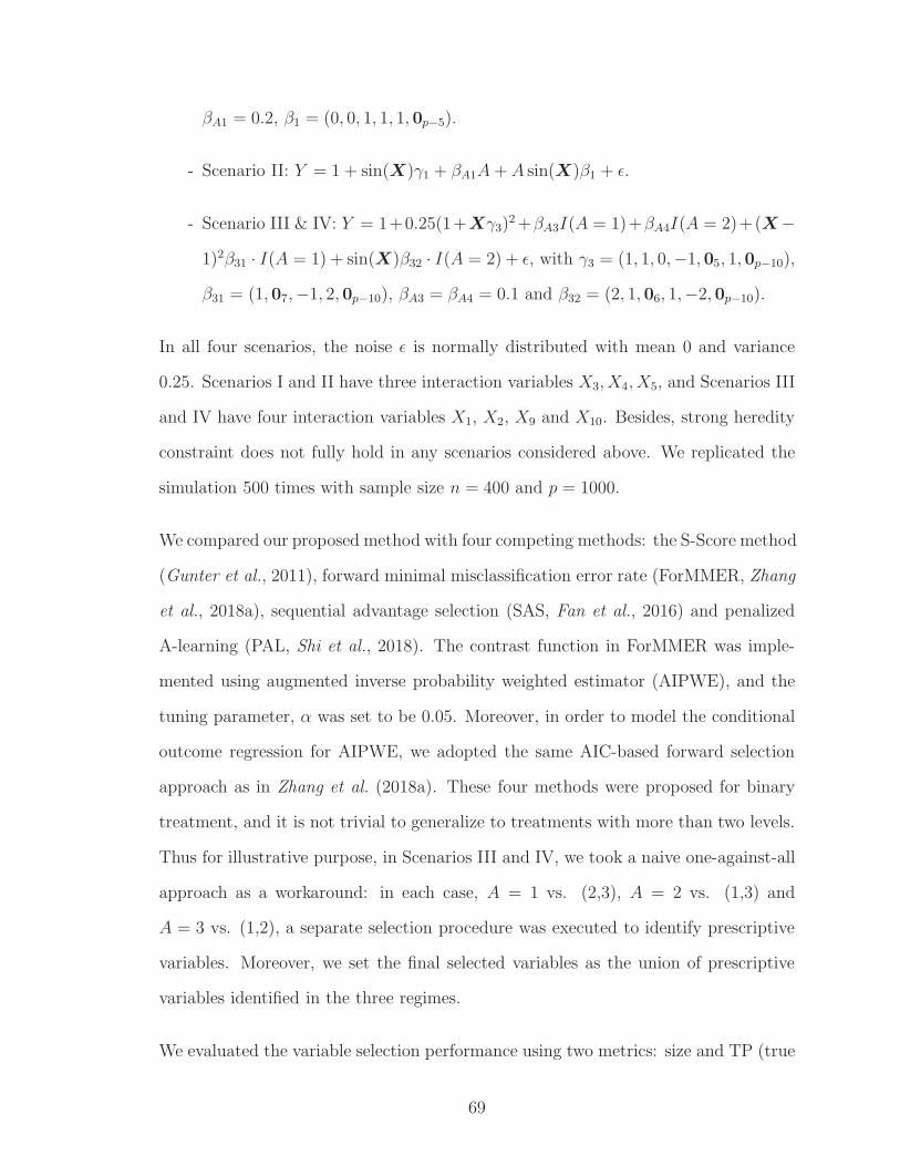
βA1 = 0.2, β1 = (0, 0, 1, 1, 1, 0p−5).
- Scenario II: Y = 1 + sin(X)γ1 + βA1A+ A sin(X)β1 + ǫ.
- Scenario III & IV: Y = 1+0.25(1+Xγ3)2+βA3I(A = 1)+βA4I(A = 2)+(X−
1)2β31 · I(A = 1) + sin(X)β32 · I(A = 2) + ǫ, with γ3 = (1, 1, 0,−1, 05, 1, 0p−10),
β31 = (1, 07,−1, 2, 0p−10), βA3 = βA4 = 0.1 and β32 = (2, 1, 06, 1,−2, 0p−10).
In all four scenarios, the noise ǫ is normally distributed with mean 0 and variance
0.25. Scenarios I and II have three interaction variables X3, X4, X5, and Scenarios III
and IV have four interaction variables X1, X2, X9 and X10. Besides, strong heredity
constraint does not fully hold in any scenarios considered above. We replicated the
simulation 500 times with sample size n = 400 and p = 1000.
We compared our proposed method with four competing methods: the S-Score method
(Gunter et al., 2011), forward minimal misclassification error rate (ForMMER, Zhang
et al., 2018a), sequential advantage selection (SAS, Fan et al., 2016) and penalized
A-learning (PAL, Shi et al., 2018). The contrast function in ForMMER was imple-
mented using augmented inverse probability weighted estimator (AIPWE), and the
tuning parameter, α was set to be 0.05. Moreover, in order to model the conditional
outcome regression for AIPWE, we adopted the same AIC-based forward selection
approach as in Zhang et al. (2018a). These four methods were proposed for binary
treatment, and it is not trivial to generalize to treatments with more than two levels.
Thus for illustrative purpose, in Scenarios III and IV, we took a naive one-against-all
approach as a workaround: in each case, A = 1 vs. (2,3), A = 2 vs. (1,3) and
A = 3 vs. (1,2), a separate selection procedure was executed to identify prescriptive
variables. Moreover, we set the final selected variables as the union of prescriptive
variables identified in the three regimes.
We evaluated the variable selection performance using two metrics: size and TP (true
69

positive). Size is the number of selected interaction variables, and TP is the number
of selected correct interaction variables. The results of the Scenarios I and II are
summarized in Table 4.1 below. In both scenarios, our proposed SpAS has stable and
outstanding performance in terms of reasonable sizes and high TPs. S-Score tends to
be conservative in terms that both methods select a small number of interactions. In
Scenario I where the correct underlying model is linear, ForMMER performs well in
terms of massive TPs. In particular, when baseline variables are weakly correlated,
ForMMER can correctly identify all the interactions in every replication. The reason
is that the AIPW estimator in ForMMER is correctly specified and therefore, the
estimated contrasts approximate the truth well. Similar to SpAS, SAS also involves
fitting conditional outcome regression models; however, SAS has much lower TPs
compared to SpAS. The reason is that SAS fits a sequence of regression models by
including one covariate at a time. Compared to the simultaneous model fitting and
variable selection in SpAS, this approach is more vulnerable to confounding effects
that are yet to be included. Also, highly correlated baseline covariates do not affect
the performance of SpAS. In Scenario II, the data generating model is non-linear, and
the working models in all competing methods are misspecified. This has a detrimental
effect on their performance. On the other hand, SpAS is still able to deliver reliable
selection results.
Table 4.2 summarizes results from Scenarios III and IV, where the outcome models
are non-linear. Note the competing methods are not directly applicable and are
included for illustrative purpose. Therefore we only demonstrated the comparison
when baseline covariates are weakly correlated. In both scenarios, SAS, ForMMER,
and S-Score all tend to over-select the interaction variables. The sizes selected by PAL
differ a lot between the two scenarios. It is worth noting that in Scenario IV, where the
treatments are randomly assigned, the competing methods have undesirable results in
terms of excessively large sizes and small TPs using the one-against-all workaround.
70

Table 4.1: Simulation results for single-stage Scenarios I and II based on 500 replica-tions. Size: number of interactions selected; TP: number of true interac-tions selected.
Weak Correlation
(ρ = 0.2)
Strong Correlation
(ρ = 0.8)
Methods Size TP Size TP
Scenario I
S-Score 1.03 (0.45) 0.84 (0.49) 1.28 (0.52) 0.69 (0.53)
ForMMER 8.72 (1.81) 3.00 (0.00) 8.67 (2.02) 2.82 (0.44)
SAS 5.09 (3.29) 2.13 (1.36) 4.03 (6.88) 1.55 (0.55)
PAL 1.44 (0.57) 1.43 (0.58) 1.10 (0.30) 1.09 (0.30)
SpAS 4.35 (0.55) 2.95 (0.33) 4.36 (0.72) 2.88 (0.34)
Scenario II
S-Score 0.87 (0.67) 0.56 (0.56) 1.17 (0.40) 0.81 (0.42)
ForMMER 2.30 (2.79) 1.21 (0.90) 4.88 (2.76) 1.24 (0.56)
SAS 0.41 (3.26) 0.13 (0.58) 3.50 (7.59) 1.39 (0.52)
PAL 1.36 (0.84) 1.11 (0.49) 1.35 (0.82) 0.97 (0.45)
SpAS 4.12 (0.72) 2.86 (0.64) 4.26 (0.65) 2.81 (0.62)
Even though in this scenario, the propensity model is guaranteed to be consistent,
the compromised performance of PAL and ForMMER could be due to the failure to
well approximate propensity scores with a large number of covariates. The proposed
SpAS results in reasonable sizes and decent TPs in both scenarios, without fitting
the model multiple times.
4.3.2 Two-stage Scenarios
We illustrated the multi-stage decision making performance of the proposed method
with two-stage Scenarios V and VI. The two scenarios have confounding variables
at both stages. The baseline variables X1 = (X1,1, · · · , X1,p1) were generated from
the same multivariate normal distribution as in Section 4.3.1. To get meaningful
comparison results, we considered binary treatments at both stages in Scenarios V
and VI. The first stage treatment A1 = 1 if X1,1 +X1,2 > 1 or X1,9 +X1,10 < 0. The
intermediate covariates collected at stage two is denoted as X2 = (X2,1, · · · , X2,p2).
71

Table 4.2: Simulation results for single-stage Scenarios III and IV based on 500 repli-cations with ρ = 0.2. The methods S-Score, ForMMER, SAS and PAL areimplemented using one-versus-all approach. Size: number of interactionsselected; TP: number of true interactions selected.
size TP
Scenario III
S-Score 51.2 (38.63) 2.24 (0.53)
ForMMER 13.74 (2.91) 3.33 (0.70)
SAS 21.22 (5.94) 3.96 (0.20)
PAL 4.72 (2.50) 2.39 (0.57)
SpAS 5.15 (1.57) 3.75 (0.41)
Scenario IV
S-Score 19.12 (42.99) 2.00 (0.54)
ForMMER 11.85 (2.40) 2.70 (0.80)
SAS 45.15 (6.15) 3.35 (0.54)
PAL 15.00 (5.43) 2.95 (0.62)
SpAS 8.37 (2.67) 3.70 (0.80)
We let p2 = 5 and X2 = 0.5 · (X1,11, · · · , X1,15)+ ǫ2, where ǫ2 ∼ N(0, 0.25). The stage
two treatment A2 = 1 if X2,3 +X2,4 < 0 or X2,1 +X2,2 < −1.
We generated the outcomes observed at the end of stage two from the following
mechanisms:
- Scenario V: Y = X1γ5,1 +X2γ5,2 + βA1A2A1A2 + A2(a2 +X2β5,2) + A1(a1 +
X1β5,1)+ ǫ, with γ5,1 = (1, 0p1−1), γ5,2 = (1, 0p2−1), βA1A2 = 4, a1 = 1, a2 = 0.5,
β5,1 = (1.55, 0p1−5), β5,2 = −2p2 .
- Scenario VI: Y = sin(X1)γ5,1+sin(X2)γ5,2+βA1A2A1A2+A2a2+cos(X2)β5,2+
A1a1 + sin(X1)β5,1+ ǫ.
The noise ǫ is normally distributed with mean 0 and variance 0.25. In Scenario
V, it is easy to see the optimal regime at the second stage is gopt2 (X1, A1,X2) =
I(βA1A2A1 + a2 +X2β5,2 > 0) and therefore is determined by six variables (A1,X2).
72

At stage one, the Q-function is
Q1(X1, A1) =EX2γ5,2 + Aopt2 (βA1A2A1 + a2 +X2β5,2)|X1, A1+X1γ5,1
+ A1(a1 +X1β5,1)
=E(βA1A2A1 + a2 +X2β5,2)+|X1, A1+ Ω(X1, A1)
=σ21√2π
exp
− µ2
1
2σ22
+ µ1[1− Φ(−µ1
σ2)] + Ω(X1, A1)
(4.5)
where Ω(X1, A1) = E(X2γ5,2|X1, A1)+X1γ5,1+A1(a1+X1β5,1), and µ1 = βA1A2A1+
a2 + 0.5 · (X1,11, · · · , X1,15). The optimal regime at stage 1 is then gopt1 (X1) =
IQ1(X1, 1) > Q1(X1, 0), and involves ten important variables (X1, · · · , X5, X11, · · · ,
X15). Note the interactions between A1 and (X1,11, · · · , X1,15) is induced by µ1, i.e.,
by assuming to follow optimal regime at stage 2. Hereafter we refer to these variables
as Q-interactions, which stand for interactions that arise from backward induction.
Following similar argument, Scenario VI has the same important interactions at both
stages.
Each Scenario was simulated 500 times with sample size n = 400 and p1 = 500.
Because S-Score was only proposed in the single-stage scenario, therefore we compared
the proposed method with ForMMER, SAS, and PAL. The results are summarized
in Table 4.3. In Scenario V, ForMMER has decent performance at stage 2 when
baseline covariates are weakly correlated; increasing correlation coefficient will result
in a drop of TP. Similar to the single-stage scenario, PAL tends to be conservative
and under-selects variables. At stage 1, all competing methods perform poorly, and
none of them (except for ForMMER in Scenario V, ρ = 0.2) have TPs fairly close
to the truth. This is due to the small magnitude of Q-interactions in the stage 1
Q-function (4.5), i.e., interactions between A1 and (X1,11, · · · , X1,15). As an empirical
verification, the column TP(µ1) in Table 4.3 suggests the competing methods are
highly unlikely to identify any Q-interactions. SpAS has an outstanding performance
73
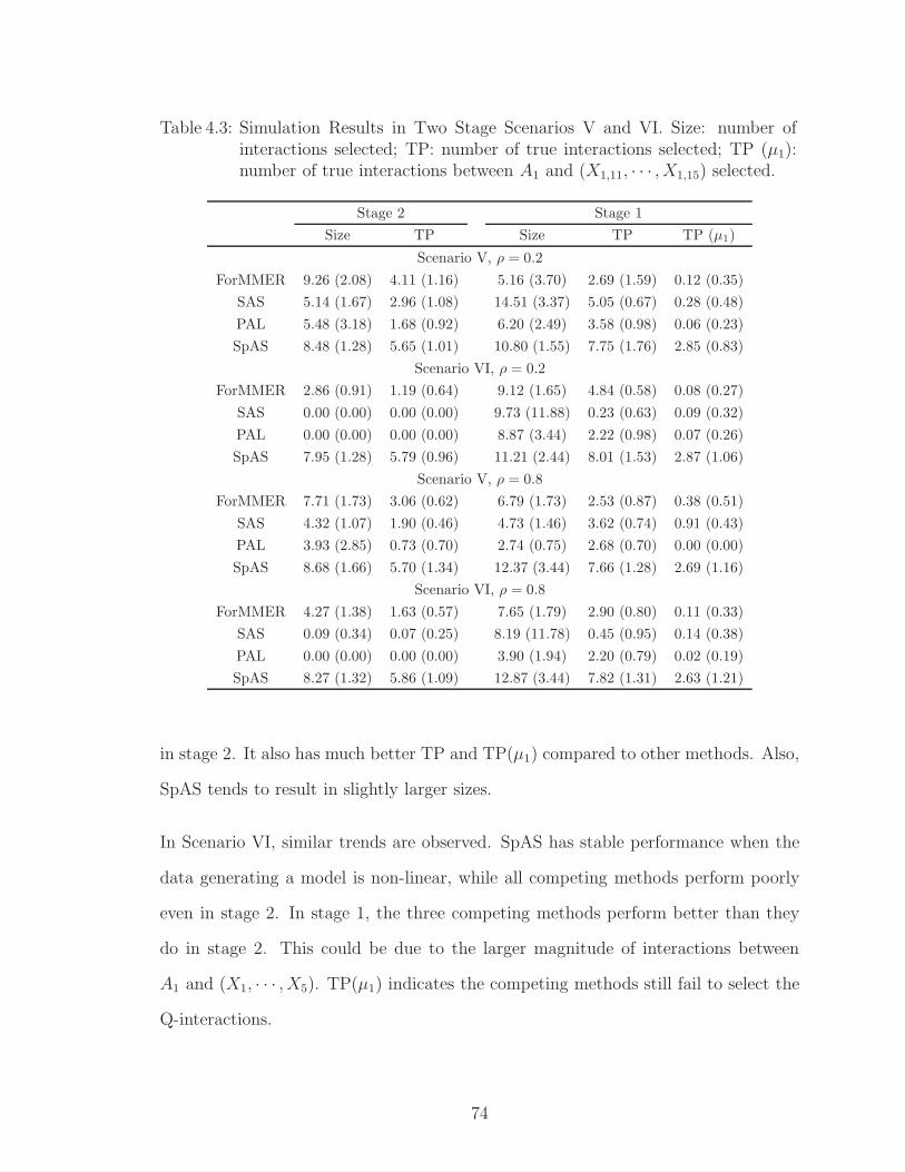
Table 4.3: Simulation Results in Two Stage Scenarios V and VI. Size: number ofinteractions selected; TP: number of true interactions selected; TP (µ1):number of true interactions between A1 and (X1,11, · · · , X1,15) selected.
Stage 2 Stage 1
Size TP Size TP TP (µ1)
Scenario V, ρ = 0.2
ForMMER 9.26 (2.08) 4.11 (1.16) 5.16 (3.70) 2.69 (1.59) 0.12 (0.35)
SAS 5.14 (1.67) 2.96 (1.08) 14.51 (3.37) 5.05 (0.67) 0.28 (0.48)
PAL 5.48 (3.18) 1.68 (0.92) 6.20 (2.49) 3.58 (0.98) 0.06 (0.23)
SpAS 8.48 (1.28) 5.65 (1.01) 10.80 (1.55) 7.75 (1.76) 2.85 (0.83)
Scenario VI, ρ = 0.2
ForMMER 2.86 (0.91) 1.19 (0.64) 9.12 (1.65) 4.84 (0.58) 0.08 (0.27)
SAS 0.00 (0.00) 0.00 (0.00) 9.73 (11.88) 0.23 (0.63) 0.09 (0.32)
PAL 0.00 (0.00) 0.00 (0.00) 8.87 (3.44) 2.22 (0.98) 0.07 (0.26)
SpAS 7.95 (1.28) 5.79 (0.96) 11.21 (2.44) 8.01 (1.53) 2.87 (1.06)
Scenario V, ρ = 0.8
ForMMER 7.71 (1.73) 3.06 (0.62) 6.79 (1.73) 2.53 (0.87) 0.38 (0.51)
SAS 4.32 (1.07) 1.90 (0.46) 4.73 (1.46) 3.62 (0.74) 0.91 (0.43)
PAL 3.93 (2.85) 0.73 (0.70) 2.74 (0.75) 2.68 (0.70) 0.00 (0.00)
SpAS 8.68 (1.66) 5.70 (1.34) 12.37 (3.44) 7.66 (1.28) 2.69 (1.16)
Scenario VI, ρ = 0.8
ForMMER 4.27 (1.38) 1.63 (0.57) 7.65 (1.79) 2.90 (0.80) 0.11 (0.33)
SAS 0.09 (0.34) 0.07 (0.25) 8.19 (11.78) 0.45 (0.95) 0.14 (0.38)
PAL 0.00 (0.00) 0.00 (0.00) 3.90 (1.94) 2.20 (0.79) 0.02 (0.19)
SpAS 8.27 (1.32) 5.86 (1.09) 12.87 (3.44) 7.82 (1.31) 2.63 (1.21)
in stage 2. It also has much better TP and TP(µ1) compared to other methods. Also,
SpAS tends to result in slightly larger sizes.
In Scenario VI, similar trends are observed. SpAS has stable performance when the
data generating a model is non-linear, while all competing methods perform poorly
even in stage 2. In stage 1, the three competing methods perform better than they
do in stage 2. This could be due to the larger magnitude of interactions between
A1 and (X1, · · · , X5). TP(µ1) indicates the competing methods still fail to select the
Q-interactions.
74

4.4 Application
We applied the proposed method to a hepatocellular carcinoma (HCC) dataset of
227 patients collected at the VA Ann Arbor Healthcare System between January
2006 and December 2013. The median follows up for this cohort is 353 days. Patient
pre-treatment objective clinical/tumor information was collected and summarized
in Table 4.4 below. Besides, 2540 body factor biomarkers were calculated using
analytic morphomics technique from pretreatment CT studies to assess patient body
composition, such as body dimensions, visceral fat, and muscle mass. Patients were
excluded if they lacked CT imaging before HCC-directed treatment, or had technical
issues with CT imaging precluding analytic morphomics.
Table 4.4: Patient Demographics in HCC Study
Age: Median (IQR) 61 (57, 66)
Race (% Caucasian) 95 (41.9%)
Etiology
Hepatitis C 167 (73.6%)
Alcohol-induced 16 (7.0%)
NASH/cryptogenic 12 (5.3%)
Multifocal HCC 110 (48.5%)
Child pugh class
A 130 (57.3)
B 70 (30.8)
C 27 (11.9)
MELD Score 9.0 (8.0, 12.0)
ECOG performance status 1.0 (0.0, 2.0)
TNM stage (I/II/III/IV) 97/49/59/22
Treatment
Resection 25 (11.1%)
TACE 83 (36.7%)
Other 118 (52.2%)
In this application, we considered three types of intervention: resection, transarte-
rial chemoembolization (TACE), and others. Besides, there are one-third censored
observations in this dataset. For illustration purpose, we imputed these censored
75

observations using a one-step approach as part of recursively imputed survival tree
algorithm (RIST, Zhu and Kosorok , 2012). Missing covariates were imputed using
hot deck imputation (Little and Rubin, 2019).
It is of interest to learn an optimal treatment rule which maximizes expected sur-
vival time by combining routine clinical information with the analytic morphomics
biomarkers; however, the limited sample size, high-dimensionality, and three-level
treatment impose challenges, and none of existing methods mentioned before can
be applied. Thus it is more realistic to conduct early-stage exploratory analyses;
one option is to identify variables that might determine optimal treatment strategy.
Therefore we analyzed this data using the proposed SpAS method to identify the
predictive and potentially prescriptive variables. We searched for tuning parameters
over a two-dimensional grid. We identified 18 main effects and 17 interaction vari-
ables. The selected variables are summarized in Table 4.5 below. The presence of a
multifocal tumor is the only prognostic variable that was not identified as a treatment
effect modifier. Besides, all clinical factors and one morphomics biomarker represent-
ing muscle measurement have been reported to be prognostic (Singal et al., 2016;
Parikh et al., 2018). Therefore, 15 new markers were identified as potential tailoring
variables, and many of them are measurements for body dimension. In addition, we
further fixed the ratio between the two tuning parameters, λ1 and λ2 to 1.5 and calcu-
lated the regularization path, as shown in Figure 4.4. Regularization path plots can
provide insight into the relative variable importance, and have important applications
in medical science. For example, sometimes, it is preferred to reduce the number of
variables being considered or collected to a certain level due to budget concern. In
such cases, the regularization path can help the investigators determine how many
and what variables to include in further research.
76

Table 4.5: The variable selection results for HCC data.
Variable nameType of
measurementInteraction
Previously
reportedDescription
SPLEENMINBBOXZ BY VISCERALFATAREA Organ Yes No The spleen size divided by the area of fat-intensity pixels in thevisceral cavity
VISCERALFATHU BY MEANPORTALVEINHU Fat Yes No Median fat pixel intensity inside the visceral cavity divided byaverage HU value on the portal vein
FASCIACIRCUMFERENCE BY VBSLABHEIGHT Body dimension Yes No Circumference of fascia perimeter divided by Height of the bodyslab for this vertebra
PSPVOLOFVB BY VB2FASCIA Muscle Yes Yes Volume of the dorsal muscle group divided by the distance betweenthe vertebra to the facial envelope
PSPVOLOFVB BY TOTALBODYAREA Muscle Yes No Volume of the dorsal muscle group divided by total body area
VISCERALFATHU BY SUBCUTFATHU Fat Yes No The ratio of median fat pixel intensities between visceral cavityand subcutaneous region
VISCERALFATHU NORMALIZED Fat Yes No Normalized median fat pixel intensity inside the visceral cavity
DIST INFANTPT2SUPANTPT Body dimension Yes No Height of the vertebral body at anterior aspect
VBSLABHEIGHT Body dimension Yes No Height of the body slab for this vertebra
VB2FRONTSKIN BY FASCIACIRCUMFERENCE Body dimension Yes No Distance from the vertebral body to the front skin divided bycircumference of fascia perimeter
SPLEENMINBBOXZ BY BODYWIDTH Organ Yes No The spleen size divided by the body width
VB2FRONTSKIN BY FASCIAAREA Body dimension Yes No Distance from the vertebral body to the front skin divided by areaof the visceral cavity
FASCIAAREA BY TOTALBODYCIRCUMFERENCE Body dimension Yes No Area of the visceral cavity divided by total body circumference
SPLEENMINBBOXZ BY VBSLABHEIGHT Organ Yes No The spleen size divided by the height of the body slab for thisvertebra
Multifocal Clinical factor No Yes Presence of multifocal tumor
Albumin Clinical factor Yes Yes Albumin
Child pugh class Clinical factor Yes Yes Child pugh class
TNM Stage Clinical factor Yes Yes TNM stage
77
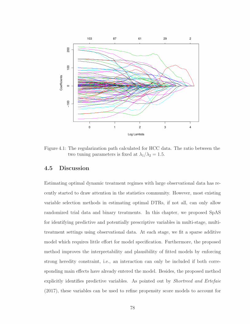
0 1 2 3 4
−1
00
01
00
20
0
Log Lambda
Co
eff
icie
nts
103 87 61 29 2
Figure 4.1: The regularization path calculated for HCC data. The ratio between thetwo tuning parameters is fixed at λ1/λ2 = 1.5.
4.5 Discussion
Estimating optimal dynamic treatment regimes with large observational data has re-
cently started to draw attention in the statistics community. However, most existing
variable selection methods in estimating optimal DTRs, if not all, can only allow
randomized trial data and binary treatments. In this chapter, we proposed SpAS
for identifying predictive and potentially prescriptive variables in multi-stage, multi-
treatment settings using observational data. At each stage, we fit a sparse additive
model which requires little effort for model specification. Furthermore, the proposed
method improves the interpretability and plausibility of fitted models by enforcing
strong heredity constraint, i.e., an interaction can only be included if both corre-
sponding main effects have already entered the model. Besides, the proposed method
explicitly identifies predictive variables. As pointed out by Shortreed and Ertefaie
(2017), these variables can be used to refine propensity score models to account for
78

confounding bias while maintaining statistical efficiency. Thus the selected predictive
variables can improve the quality of estimated dynamic treatment regime.
Qian and Murphy (2011) studied the mismatch between minimizing squared error
loss when fitting outcome regression models and maximizing the mean counterfactual
outcome when learning the optimal treatment regimes. In response, recently, there
has been a surge of direct methods for estimating optimal DTRs. Likewise, in this
area, all existing variable selection methods directly target at optimizing the mean
counterfactual outcome based on models for contrast in outcome regression between
two treatment levels. Such a strategy does not solve the challenge of how to construct
working models, especially when p ≫ n. Nevertheless, these methods are restricted
to binary treatment by their nature. On the contrary, our proposed method is ap-
pealing in terms that it allows multi-level treatments and continuous doses, as well
as observational data.
It is still worth noting that SpAS selects treatment effect modifiers, which are not nec-
essarily tailoring variables. Therefore the proposed method would result in a larger
set of variables. However, once the number of selected variables becomes manageable,
domain experts can help further narrow down the variable list to improve the quality
of estimated DTRs and/or to achieve cost-effectiveness. In addition, choosing the
optimal tuning parameter is crucial. The proposed method uses the high-dimensional
BIC for model tuning; however, this criterion was not specifically proposed for our
purpose. It is of both theoretical and practical interest to further study the perfor-
mance of available metrics or to develop new metrics for parameter tuning in variable
selection for estimating optimal DTRs.
79

CHAPTER V
Summary and Future Work
In this dissertation, we have explored some flexible modeling strategies for coarsened
data problems including nonparametric kernel regression when the outcome is missing
at random (MAR) and estimating interpretable optimal dynamic treatment regimes
using observational data. The overarching goal is to develop flexible, easy-to-use
statistical methods while improving model robustness.
The MRKEE method proposed in Chapter II is an essential addition to the literature
of multiple robustness. It achieves consistency when any one of missing mechanism
or conditional outcome regression models is known or can be correctly specified, thus
provides more protection against working model misspecification. MRKEE also has
great potential in applications such as flexible dose-response modeling when data are
subject to missingness, which is often the case in radiation oncology. Chapter III and
IV studied the role of nonparametric machine learning methods in estimating opti-
mal dynamic treatment regimes using observational data. The use of such powerful
tools further relaxes model assumptions and requires minimal guesswork in model
specification. The ST-RL method proposed in Chapter III estimates optimal DTRs
as a sequence of decision trees, one per stage, and thus are interpretable to clinicians
and human experts. It also scales well to a moderately large number of covariates.
Chapter III contributes to theory development regarding the finite sample bounds
80

when using non-greedy tree search algorithm for estimating optimal DTRs. The
variable selection method proposed in Chapter IV can identify potential predictive
and prescriptive variables when more than two treatment options are available using
observational data.
Some extensions can further enhance the versatility of nonparametric regression in
the presence of missing data. First of all, it is of interest to extend MRKEE to allow
multiple predictors as this is often the case in practice. It is also vital to extend
MRKEE to accommodate other common types of outcomes, such as binary, time-to-
event, and longitudinal data.
One important future research direction of ST-RL is to allow continuous treatment,
such as radiation doses. Although there has been some exploration of optimal dosing
strategy (e.g., Laber and Zhao, 2015; Chen et al., 2016), existing methods are com-
putationally demanding and lacking satisfactory empirical performance. Therefore it
is still of great interest to develop dynamic treatment regimes for multi-stage dose
optimization. Furthermore, the time-to-event outcome is often of interest in clinical
studies. The statistics community only recently started to focus on optimal DTR esti-
mation using survival data (e.g., Jiang et al., 2017; Hager et al., 2018; Simoneau et al.,
2019). Extending our tree-based method to survival outcome can greatly improve the
interpretability of estimated DTRs.
In high-dimensional setting, especially p ≫ n, we explored the variable selection
method in Chapter V to facilitate the construction of optimal DTRs. Similar to
ST-RL, the extension to accommodate survival outcome is also of great importance.
Another important research direction is to further relax the additivity assumption by
considering a more flexible regression framework.
81

APPENDICES
82

APPENDIX A
Proofs for Chapter II
Lemma 1.1. When π1(ν1) is the correctly specified model for Pr(R = 1|Z,U) and
ν10 is the true parameter value, we have
√nhλ = (nh)1/2M−1 1
n
n∑
i=1
Ri − π1
i (ν10)
π1i (ν
10)
gi(ν∗,α∗,γ∗)
+ op(1).
where M is given by (2.12) and g(ν∗,α∗,γ∗) is given by (2.11).
Proof of Lemma. We first show that the asymptotic distribution of λ stays the
same whether π10 is known or can be estimated consistently at
√n-rate, i.e.
√n(ν1−
ν10) = Op(1). Suppose, under some regularity conditions, ∂θMRz; π(ν1)/∂ν1T is
bounded in a neighborhood of ν10, i.e.,
∂θMRz; π(ν1)/∂ν1T|ν1∈N (ν10)= Op(1),
83

where N (ν10)⊃ν1 : ||ν1 − ν1
0||< ||ν1 − ν10||. We have
√nh[θMRz; π(ν1) − θ(z)]
=√nh[θMRz; π(ν1) − θMRz; π(ν1
0)] +√nh[θMRz; π(ν1
0) − θ(z)]
=√h
[∂θMRz; π(ν1)
∂ν1T|ν1∗
]√n(ν1 − ν1
0) +√nh[θMRz; π(ν1
0) − θ(z)] (A.1)
for some ν1∗ ∈ ν1 : ||ν1 − ν10||< ||ν1 − ν1
0||. Note√n(ν1 − ν1
0) = Op(1),
∂θMR z; π(ν1) /∂ν1T|ν1∗= Op(1), and h → 0 as n → ∞, the first term in (A.1)
is op(1). Therefore, the asymptotic distribution of θMRz; π(ν1) when ν1 is esti-
mated consistently at√n-rate is the same as that of θMR(z; π0) when π0 is known.
Similar argument shows that the asymptotic results remain the same if (ν, γ) is
replaced with its probability limit (ν∗, γ∗). Taking Taylor expansion of the left-hand
side of (2.9) around (0T,αT∗ ) leads to
0 = (nh)1/21
n
n∑
i=1
Ri
π1i (ν
10)gi(ν∗,α∗,γ∗)−
1
n
n∑
i=1
Ri
π1i (ν
10)
gi(ν∗,α∗,γ∗)⊗2
π1i (ν
10)
(nh)1/2λ
+
K∑
k=1
1
n
n∑
i=1
Ri
π1i (ν
10)
0J+2(k−1)×2
∂ψk
i(αk
∗,γk
∗)
∂αk − 1n
∑nh=1
∂ψk
h(αk
∗,γk
∗)
∂αk
02(K−k)×2
(nh)1/2(αk −αk∗)
= (nh)1/21
n
n∑
i=1
Ri
π1i (ν
10)gi(ν∗,α∗,γ∗)− (nh)1/2Mλ+ op(1).
On the other hand, it is easy to check that
(nh)1/21
n
n∑
i=1
Ri
π1i (ν
10)gi(ν∗,α∗,γ∗) = (nh)1/2
1
n
n∑
i=1
Ri − π1i (ν
10)
π1i (ν
10)
gi(ν∗,α∗,γ∗) + op(1).
Then, solving for λ from the above Taylor expansion gives the result.
84

Proof of Theorem 2. From the previous proof, we can replace (ν, γ) estimated at
√n-rate by its probability limit (ν∗,γ∗) without affecting the asymptotic distribution.
Since αMR satisfies
0 =
m∑
i=1
wiφi(αMR) =1
m
n∑
i=1
RiΠ1(ν1)/π1
i (ν1)
1 + λTgi(ν, α, γ)/π
1i (ν
1)φi(αMR),
we have
0 =1
m
1
n
n∑
h=1
π1h(ν
10)
(nh)1/2
n∑
i=1
Ri
π1i (ν
10)φi(α0)
− 1
m
1
n
n∑
h=1
π1h(ν
10)
n∑
i=1
Ri
π1i (ν
10)φi(α0)
gi(ν∗,α∗,γ∗)T
π1i (ν
10)
(nh)1/2λ
+1
m
1
n
n∑
h=1
π1h(ν
10)
n∑
i=1
Ri
π1i (ν
10)
∂φi(α0)
∂αT
(nh)1/2(αMR −α0) + op(1)
=√n1
n
n∑
i=1
Ri
π1i (ν
10)
√hφi(α0)−
√nLλ+ E
∂φ(α0)
∂αT
(nh)1/2(αMR −α0) + op(1)
=1√n
n∑
i=1
Qi(z) + E
∂φ(α0)
∂αT
(nh)1/2(αMR −α0) + op(1).
We suppress the denpendence of Qi(z) on z and denote it as Qi. We then have
0 =1√n
n∑
i=1
Qi + E
∂φ(α0)
∂αT
(nh)1/2(αMR −α0) + op(1).
Solving for√nh(αMR −α0) leads to
√nhαMR −α0 = −
[E
∂φ(α0)
∂αT
]−11√n
n∑
i=1
Qi,
which gives WMR,π(z).
85

The bias term can be derived as follows. We expand the derivative term:
E
∂φ(α0)
∂α
= E
[Kh(Z − z)
µ(1)(z,α0)
2V −1(z,α0)G(Z − z)G(Z − z)T
]+ op(1)
= −fZ(z)(µ(1)θ(z)
)2V −1θ(z)D(K) + op(1)
where D (K) is a 2 × 2 matrix with the (j, k)th element cj+k−2(K) × h(j+k−2), and
cr(K) =∫srK(s)ds.
Moreover, we rewrite 1√n
∑ni=1Qi =
√nh · 1
n
∑ni=1Qi/
√h =√nh · (Q1n+Q2n−Q3n),
where
Q1n = n−1n∑
i=1
Ri
π1i0
Kh(Zi − z)µ(1)i (z,α0)V
−1i (z,α0)G(Zi − z) [Yi − µθ(Zi)]
Q2n = n−1n∑
i=1
Ri
π1i0
Kh(Zi − z)µ(1)i (z,α0)V
−1i (z,α0)G(Zi − z)
[µθ(Zi) − µG(Zi − z)Tα0
]
Q3n = n−1
n∑
i=1
Ri − π1i0
π1i0
LM−1gi(ν∗,α∗,γ∗).
It is easily seen that when π1(ν1) is correctly specified, Q1n and Q3n are asymptot-
ically normal with mean zero. Therefore, Q2n is the leading bias term, and under
MAR we have bias Q2n =
EKh(Z − z)µ(1)(z,α0)V
−1(z,α0)[µ θ(Z) − µ
G(Z − z)Tα0
]G(Z − z)
+ op(1)
=1
2θ′′(z)
[µ(1)θ(z)
]2V −1θ(z)fZ(z)H(K) + o(h2),
where H(K) is a 2× 1 vector with the kth element ck+1(K)× h(k+1). Note that the
variance of Q2n is of order o(1/nh), and hence can be ignored asymptotically.
86

Proof of Theorem 3. Write
H =R
π1(ν10)
√hφ(α0), A =
R
π1(ν10)g(ν∗,α∗,γ∗).
It is easy to check that L = E(HAT) andM = E(A⊗2). Now P contains a correctly
specified model for P (R = 1|Z,U) (denoted as π1(ν10)). When A contains a correctly
specified model for E(Y |Z,U) (denoted as a1(γ10)), E
√hφ(α0)|Z,U is a component
of g(ν∗,α∗,γ∗), and thus E√hφ(α0)|Z,UR/π1(ν1
0) is in the linear space spanned
by A. Since
E
([H − R
π1(ν10)E√hφ(α0)|Z,U
]R
π1(ν10)f(Z,U)
)= 0
for any function f(Z,U) and all components of g(ν∗,α∗,γ∗) are functions of Z and
U only, we have that
LM−1A = E(HAT)E(A⊗2)−1A =R
π1(ν10)E√hφ(α0)|Z,U.
This fact yields that LTM−1g(ν∗,α∗,γ∗) = E√hφ(α0)|Z,U, and thus
Q =R
π1(ν10)
√hφ(α0)−
R− π1(ν10)
π1(ν10)
E√hφ(α0)|Z,U.
Similar to previous proof, we write 1√n
∑ni=1Qi =
√nh · 1
n
∑ni=1Qi/
√h =
√nh ·
(Q1n +Q2n −Q3n), where Q1n is the same as in the previous proof, and
Q2n = n−1n∑
i=1
Ri
π1i (ν
10)−1Kh(Zi−z)µ(1)
i (z,α0)V−1i (z,α0)
[a1i (γ
10)− µθ(Zi)
]G(Zi−z),
and
Q3n = n−1n∑
i=1
Kh(Zi−z)µ(1)i (z,α0)V
−1i (z,α0)
[µθ(Zi) − µG(Zi − z)Tα0
]G(Zi−z).
87

It is easily seen that Q1n and Q2n have mean 0. The third term Q3n is the leading
bias term, and simple calculations show that E [Q3n] is equal to (A.2). It follows that
biasαMR(z) =1
2h2θ′′(z)c2(K) + o(h2).
Note that the variance of Q3n is of order o(1/nh), and hence can be ignored asymp-
totically. When both P and A contain a correctly specified model, Q1n + Q2n is
asymptotically normal with mean 0 and variance
Var Q1n +Q2n =1
nVar
Q1,2
,
where
Q1,2 = Kh(Z − z)µ(1)(z,α0)V−1(z,α0)G(Z − z)
×(
R
π1(ν10)
[Y − µθ(Z)]−
R
π1(ν10)− 1
[a1(γ1
0)− µθ(Z)])
Further calculation shows that n−1VarQ1,2
equals
1
nE
[K2
h(Z − z)µ(1)(z,α0)
2V −2(z,α0)G(Z − z)G(Z − z)T
×(
R
π1(ν10)
[Y − µθ(Z)]−
R
π1(ν10)− 1
[a1(γ1
0)− µθ(Z)])2],
which can be simplified as
1
nhfZ(z)
[µ(1)θ(z)
]2V −2θ(z)E
[Var(Y |Z,U)
π0(Z,U)
+ [E(Y |Z,U)− µθ(Z)]2∣∣Z = z
]D(K2) + o(
1
nh)
88

Summarizing all these results gives Theorem 3.
89

APPENDIX B
Proofs for Chapter III
Proof of Theorem 3.1. Let us consider one-stage case for now. Our proof is a
direct extension of Rockova and van der Pas (2017) (refer to as RP17 hereafter).
Since we stochastically search optimal regime using Bayesian CART algorithm, it
is sufficient to prove that Pr(s & nd0H/2α+d0
H |H, Aopt) → 0, where d0H
is the number
of signal variables in the true tree-structured regime that assigns patients to Aopt.
The sieve Fn, consisting of step functions over small trees that split only on a few
variables, can be constructed for given n ∈ N consisting of step functions over small
trees (sn) that split only on a few (qn) variables using the same way as in RP17:
Fn =
qn⋃
q=0
sn⋃
s=1
⋃
H:dH=q
F(VsH),
where |dH| is the number of variables in H that actually determine the decision rules,
and VsH
denotes a family of valid tree partitions with s leaves based on H variables.
The set of step functions supported by VsH
is then defined as
F(VsH) =
fT ,β : [0, 1]p → (1, · · · , K); fT ,β(H) =
s∑
l=1
βlIΩl(H); T ∈ Vs
H,β ∈ (1, · · · , K)s
.
90

Denote the conditional probabilities (η1,···,K) = Pr(Aopt = 1, · · · , K|H), and (η∗1,···,K)
denotes the conditional probabilities under true data generating process. Define met-
ric d(f, f ∗) =√∑K
k=1||ηk − η∗k||2n. Therefore for sets Fn ⊂ F , we want to show
Π(F \ Fn) = o(e−(δ+2)nǫ2n), where sequence ǫ2n → 0 and nǫ2n is bounded away from 0,
and δ > 0 satisfies
supǫn>ǫ
logN(ǫ/36, f ∈ Fn : d(f, f ∗) < ǫn, d(·, ·)) ≤ nǫ2n, (B.1)
Π(f ∈ Fn : d(f, f ∗) ≤ ǫn) ≥ e−δnǫ2n . (B.2)
The ǫ-covering numbers of the set f : d(f, f ∗) ≤ ǫ for d(·, ·) is bounded by the
ǫ√n/C-covering numbers of a Euclidean ball η ∈ [0, 1]s×K = (η1,···,K) ∈ [0, 1]s :
√∑Kk=1||ηk − η∗
k|||22 ≤ ǫ√n/C. The tree size and variable dimensions that define
the sieve can be selected as qn = ⌈CmindH, nq0/(2α+q0) log2β n/log(p∨n)⌉ and sn =
⌊C ′nǫ2n/logn⌋ ≍ nq0/(2α+q0) log2β−1 n.
It can be seen that Π(F \ Fn) < Π(s > sn) + Π(q > qn). Using the same arguments
as in Section 8.3 of RP17 completes the proof by showing Π(s > sn) ≍ o(e−(δ+2)nǫ2n)
and Π(s > sn) ≍ o(e−(δ+2)nǫ2n).
The proof of Theorem 3.2 requires several ancillary results shown below.
The following lemma is a modified version of Theorem 7.1 in Rockova and van der
Pas (2017), which provides the finite sample bound of BART. Note the convergence
is evaluated for E(Y |A,H), not Q, and they are not equivalent except at the last
stage.
Proof. Since ||f ||∞ and ||f0||∞ are bounded, we can verify ||f − f0||42< ∞. Then by
91

Bernstein’s inequality (Christmann and Steinwart , 2008), we have
Pr(∣∣∣Pn||f − f0||22−E||f − f0||22
∣∣∣ & τ/n +√τ/n
)≤ e−τ .
Moreover, under the assumptions, Rockova and van der Pas (2017) showed that with
probability approaching 1, ||f − f0||n. n− α
2α+dH log1/2 n. Therefore we plug in this
result, and
Pr(E||f − f0||22& n
− 2α2α+dH log n+ τ/n
)≤ e−τ .
The following lemma establishes the convergence rate of Qt, t = 1, · · · , T .
Theorem 2.1. Suppose the assumptions in Section 3 hold, PrPn(Yt − ˆ
Y t)2 & τn−ζ
≤
e−τ , where ξ, ζ > 0, then it follows
Pr
(E||Qt −Qt||22& n
− 2αt2αt+dHt logn + τn−min(1,ζ)
)≤ e−τ .
Proof. Recall Qt = E(ˆY t|At,Ht), and Qt = E(Yt|At,Ht). To facilitate the proof, we
denote Qnt = E(
ˆY t|At,Ht). Then we have
E||Qt −Qt||22≤ E||Qt −Qnt ||22+E||Qn
t −Qt||22.
To bound the second term, define Zt ≡ ˆY t−Yt, thus Qn
t −Qt = E(Zt|At,Ht). Consider
the regression model Zt = E(Zt|At,Ht)+ǫ. It can be seen ||Zt||22≥ ||E(Zt|At,Ht)||22−||ǫ||22and ||ǫ||22= Op(1), then ||Qn
t − Qt||22. ||Zt||22. As a result, and again by Bernstein’s
inequality, E||Qt −Qt||22. E||Zt||22+E||f − f0||22, and
92

Pr
(E||Qt −Qt||22& n
− 2αt2αt+dHt log n+ τn−min(1,ζ)
)≤ e−τ .
With these results, now we prove Theorem 3.2.
Proof of Theorem 3.2. For finite sample bound derivation, we assume the data are
bounded, i.e. there exist some B ∈ R+ such that ||Y ||∞< B. We start from the
final stage T and omit the subscript notation for stage now. Using the triangular
inequality, we have
Pr(gopt 6= g∗opt) ≤K∑
i=1
Pr(Ai 6= A∗i ) + d(p,p∗). (B.3)
One can easily notice that
K∑
i=1
Pr(Api 6= A∗pi)
≤Pr
supp∈σ(T ),Ap 6=A∗
p
PnF (p,Ap) ≥ PnF (p∗,A∗
p)
≤Pr
supp∈σ(T )
∣∣∣PnF (p,Ap)− EF (p,Ap)∣∣∣ ≥ τ/2
.
(B.4)
The second inequality holds because in assumptions we assume for arbitrarily small
τ , EF (p∗,A∗p) ≥ supp∈σ(T ),Ap 6=A∗
pEF (p,Ap) + τ .
93

In order to bound this probability, we write
supp∈σ(T )
|PnF (p,Ap) − EF (p,Ap)|
≤ supp∈σ(T )
|PnF (p,Ap) − PnF (p,Ap)|+ supp∈σ(T )
|PnF (p,Ap) − EF (p,Ap)|.
The first term can then be bounded:
supp∈σ(T )
|PnF (p,Ap) − PnF (p,Ap)|
≤ supp∈σ(T )
|Pn
Kt∑
a=1
[Qt(a,Ht)−Qt(a,Ht)
] Kt∑
i=1
I(Ht ∈ pit)I(Ait = a)|
≤|Pn
K∑
i=1
[Q(i,H)−Q(i,H)
]|
≤K∑
i=1
Pn
[Q(i,H)−Q(i,H)
]21/2
.n− α2α+p log1/2 n.
The second term can be bounded by the property of VC-class. Following the argu-
ments in Zhang et al. (2018b), we have
Pr
sup
p∈σ(T )
|PnF (p,Ap) − EF (p,Ap)|& 1/√n+
√τ/n
≤ e−τ
up to a constant determined by the VC index. Therefore, it follows that
Pr
sup
p∈σ(T )
∣∣∣PnF (p,Ap)− EF (p,Ap)∣∣∣ & n− α
2α+p log1/2 n
≤ e−τ , (B.5)
and consequently (B.4) becomes∑K
i=1 Pr(Api 6= A∗pi) . exp(n
α2α+p/log1/2 n).
94

In order to bound d(p, p∗), we first look at
supp∈σ(T ),d(p,p∗)≤d
∣∣∣PnF (p,A∗)− EF (p,A∗)−
PnF (p
∗,A∗)− EF (p∗,A∗)∣∣∣ (B.6)
≤ supp∈σ(T ),d(p,p∗)≤d
|PnF (p,A∗)− EF (p,A∗)− PnF (p
∗,A∗)− EF (p∗,A∗)| (B.7)
+ supp∈σ(T ),d(p,p∗)≤d
∣∣∣PnF (p,A)− PnF (p,A)−PnF (p
∗,A)− PnF (p∗,A)
∣∣∣ . (B.8)
The first term (B.7) (denoted as T6) can be bounded using VC class property. Again
by VC preservation theorem,
Fd =
K∑
i=1
Q(Api ,H)−Q(Ap∗i,H)I(H ∈ pi p∗i ) : p ∈ σ(T ), d(p, p∗) ≤ d
is also VC class. Also because ||f ||∞≤ 2B for ∀f ∈ Fd and V ar(f) ≤ Ef 2 ≤ dB2, by
concentration inequality we have
Pr
||Pnf − Ef ||∞&
[d1/2 log1/2(1/d) + d1/2τ 1/2√
n+
log(1/d) + τ
n
]≤ e−τ ,
and by applying log(1/d) . d−δ for ∀δ ∈ R+,
PrT6 & d1/2−δ(n−1/2 + n−1/2τ 1/2) + d−δ(n−1 + n−1τ) ≤ e−τ . (B.9)
95

To bound the second term (B.8) (denoted as T7), we have
T7 ≤∣∣∣∣∣Pn
K∑
i=1
Q(Api,H)− Q(Ap∗i,H)I(H ∈ pi p∗i )
−K∑
i=1
Q(Api ,H)−Q(Ap∗i,H)I(H ∈ pi p∗i )
∣∣∣∣∣
≤∣∣∣∣∣Pn
K∑
i=1
Q(Api,H)−Q(Api ,H)I(H ∈ pi p∗i )
−K∑
i=1
Q(Ap∗i,H)−Q(Ap∗i
,H)I(H ∈ pi p∗i )
∣∣∣∣∣ ,
where pi p∗i denotes the symmetric difference, equivalent to pi ∪ p∗i /pi ∩ p∗i . We
further let ǫ =∑K
i=1[EQ(Ap∗i,H)−Q(Ap∗i
,H)2]1/2. Now it follows
E
K∑
i=1
Q(Ap∗i,H)−Q(Ap∗i
,H)I(H ∈ pi p∗i )
≤K∑
i=1
E[Q(Ap∗i,H)−Q(Ap∗i
,H)I(H ∈ pi p∗i )]
≤K∑
i=1
[EQ(Ap∗i,H)−Q(Ap∗i
,H)2]1/2[EI(H ∈ pi p∗i )]1/2
≤d1/2ǫ.
As a result ET7 . d1/2ǫ. We further notice that its variance can be bounded by c′d.
Therefore, by concentration inequalities,
PrT7 & d1/2−δ(ǫ+ n−1/2 + n−1/2τ 1/2) + d−δ(n−1 + n−1τ) ≤ e−τ .
Now we take a look at quantity (B.6), hereby denoted as T5:
PrT5 & n− α2α+p log1/2 nτ ≤ e−τ .
96

By Lemma 18 in Zhang et al. (2018b), Prd(p,p∗) & τn−2/3 α2α+p log1/2 n ≤ e−τ .
Thus at stage T , we have Pr(goptT 6= goptT ) . n−2/3
αT2αT +dHT log1/2 n . n−rT+ǫ, and
Pr(V (goptT )− V (goptT ) & τn−rT+ǫ) ≤ e−τ .
For stage t = T − 1, we have Pr(||Yt − ˆY t||n& τn−rT+ǫ) ≤ e−τ , then by Lemma 2.1,
one can easily get
Pr
(E||Qt −Qt||22& n
− 2αt2αt+dHt log n+ τn−2rT+ǫ
)≤ e−τ ,
i.e. Pr(E||Qt −Qt||22& τn
−2min(αt
2αt+dHt,rT )+ǫ
)≤ e−τ , i.e. the rate depends on the con-
vergence rate of BART assuming Yt is observed, and also depends on the convergence
rate carried over from previous stage estimations. Using similar arguments, we have
Pr(goptt 6= goptt ) . n−2/3min(
αt2αt+dHt
,rT )log1/2 n . n−rt+ǫ, and Pr(V (goptT ) − V (goptT ) &
τn−rts+ǫ) ≤ e−τ .
Similarly, results can be obtained for all t.
97

BIBLIOGRAPHY
98

BIBLIOGRAPHY
Ajani, J., et al. (2013), A phase ii randomized trial of induction chemotherapy versusno induction chemotherapy followed by preoperative chemoradiation in patientswith esophageal cancer, Annals of oncology, 24 (11), 2844–2849.
Bien, J., J. Taylor, and R. Tibshirani (2013), A lasso for hierarchical interactions,Annals of statistics, 41 (3), 1111.
Breiman, L. (2001), Random forests, Machine learning, 45 (1), 5–32.
Chan, K. C. G., S. C. P. Yam, et al. (2014), Oracle, multiple robust and multipurposecalibration in a missing response problem, Statistical Science, 29 (3), 380–396.
Chang, M., S. Lee, and Y.-J. Whang (2015), Nonparametric tests of conditional treat-ment effects with an application to single-sex schooling on academic achievements,The Econometrics Journal, 18 (3), 307–346.
Chen, G., D. Zeng, and M. R. Kosorok (2016), Personalized dose finding using out-come weighted learning, Journal of the American Statistical Association, 111 (516),1509–1521.
Chen, J., R. Sitter, and C. Wu (2002), Using empirical likelihood methods to obtainrange restricted weights in regression estimators for surveys, Biometrika, 89 (1),230–237.
Chen, S., and D. Haziza (2017), Multiply robust imputation procedures for the treat-ment of item nonresponse in surveys, Biometrika, 104 (2), 439–453.
Chipman, H. A., E. I. George, and R. E. McCulloch (1998), Bayesian cart modelsearch, Journal of the American Statistical Association, 93 (443), 935–948.
Chipman, H. A., E. I. George, R. E. McCulloch, et al. (2010), Bart: Bayesian additiveregression trees, The Annals of Applied Statistics, 4 (1), 266–298.
Choi, N. H., W. Li, and J. Zhu (2010), Variable selection with the strong heredityconstraint and its oracle property, Journal of the American Statistical Association,105 (489), 354–364.
Christmann, A., and I. Steinwart (2008), Support vector machines.
99

Day, D. B., et al. (2017), Association of ozone exposure with cardiorespiratory patho-physiologic mechanisms in healthy adults, Jama Internal Medicine, 177 (9), 1344–1353.
Denison, D. G., B. K. Mallick, and A. F. Smith (1998), A bayesian cart algorithm,Biometrika, 85 (2), 363–377.
Deville, J.-C., and C.-E. Sarndal (1992), Calibration estimators in survey sampling,Journal of the American statistical Association, 87 (418), 376–382.
Donnelly, A., B. Misstear, and B. Broderick (2011), Application of nonparametricregression methods to study the relationship between no 2 concentrations and localwind direction and speed at background sites, Science of the Total Environment,409 (6), 1134–1144.
Duda, R. O., P. E. Hart, and D. G. Stork (2012), Pattern classification, John Wiley& Sons.
Fan, A., W. Lu, and R. Song (2016), Sequential advantage selection for optimaltreatment regime, The annals of applied statistics, 10 (1), 32.
Gail, M., and R. Simon (1985), Testing for qualitative interactions between treatmenteffects and patient subsets., Biometrics, 41 (2), 361–372.
Gao, X., and R. J. Carroll (2017), Data integration with high dimensionality,Biometrika, 104 (2), 251–272.
Gill, R. D., M. J. Van Der Laan, and J. M. Robins (1997), Coarsening at random:Characterizations, conjectures, counter-examples, in Proceedings of the First SeattleSymposium in Biostatistics, pp. 255–294, Springer.
Giorgini, P., et al. (2015a), Higher fine particulate matter and temperature levelsimpair exercise capacity in cardiac patients, Heart, pp. heartjnl–2014.
Giorgini, P., et al. (2015b), Particulate matter air pollution and ambient tempera-ture: opposing effects on blood pressure in high-risk cardiac patients, Journal ofhypertension, 33 (10), 2032–2038.
Gunter, L., J. Zhu, and S. Murphy (2011), Variable selection for qualitative interac-tions, Statistical methodology, 8 (1), 42–55.
Hager, R., A. A. Tsiatis, and M. Davidian (2018), Optimal two-stage dynamic treat-ment regimes from a classification perspective with censored survival data, Biomet-rics, 74 (4), 1180–1192.
Han, P. (2014a), A further study of the multiply robust estimator in missing dataanalysis, Journal of Statistical Planning and Inference, 148, 101–110.
Han, P. (2014b), Multiply robust estimation in regression analysis with missing data,Journal of the American Statistical Association, 109 (507), 1159–1173.
100

Han, P. (2016a), Combining inverse probability weighting and multiple imputation toimprove robustness of estimation, Scandinavian Journal of Statistics, 43, 246–260.
Han, P. (2016b), Combining inverse probability weighting and multiple imputationto improve robustness of estimation, Scandinavian Journal of Statistics, 43 (1),246–260.
Han, P., and L. Wang (2013), Estimation with missing data: beyond double robust-ness, Biometrika, 100 (2), 417–430.
Heitjan, D. F. (1993), Ignorability and coarse data: Some biomedical examples, Bio-metrics, pp. 1099–1109.
Hill, J. L. (2011), Bayesian nonparametric modeling for causal inference, Journal ofComputational and Graphical Statistics, 20 (1), 217–240.
Hirano, K., G. W. Imbens, and G. Ridder (2003), Efficient estimation of averagetreatment effects using the estimated propensity score, Econometrica, 71 (4), 1161–1189.
Horvitz, D. G., and D. J. Thompson (1952), A generalization of sampling withoutreplacement from a finite universe, Journal of the American statistical Association,47 (260), 663–685.
Hsu, Y.-C. (2017), Consistent tests for conditional treatment effects, The economet-rics journal, 20 (1), 1–22.
Huang, X., S. Choi, L. Wang, and P. F. Thall (2015), Optimization of multi-stage dy-namic treatment regimes utilizing accumulated data, Statistics in medicine, 34 (26),3424–3443.
Jiang, R., W. Lu, R. Song, and M. Davidian (2017), On estimation of optimal treat-ment regimes for maximizing t-year survival probability, Journal of the Royal Sta-tistical Society: Series B (Statistical Methodology), 79 (4), 1165–1185.
Kang, J. D., J. L. Schafer, et al. (2007), Demystifying double robustness: A com-parison of alternative strategies for estimating a population mean from incompletedata, Statistical science, 22 (4), 523–539.
Kennedy, E. H., W. L. Wiitala, R. A. Hayward, and J. B. Sussman (2013), Improvedcardiovascular risk prediction using nonparametric regression and electronic healthrecord data, Medical care, 51 (3), 251.
Kim, J., D. Pollard, et al. (1990), Cube root asymptotics, The Annals of Statistics,18 (1), 191–219.
Kosorok, M. R. (2008), Introduction to empirical processes and semiparametric infer-ence., Springer.
101

Laber, E., and Y. Zhao (2015), Tree-based methods for individualized treatmentregimes, Biometrika, 102 (3), 501–514.
Laurent, H., and R. L. Rivest (1976), Constructing optimal binary decision trees isnp-complete, Information processing letters, 5 (1), 15–17.
Linero, A. R. (2018), Bayesian regression trees for high-dimensional prediction andvariable selection, Journal of the American Statistical Association, 113 (522), 626–636.
Linero, A. R., and Y. Yang (2018), Bayesian regression tree ensembles that adapt tosmoothness and sparsity, Journal of the Royal Statistical Society: Series B (Statis-tical Methodology), 80 (5), 1087–1110.
Little, R., and D. Rubin (2002), Statistical analysis with missing data, Wiley, Hobo-ken.
Little, R. J. (1992), Regression with missing x’s: a review, Journal of the AmericanStatistical Association, 87 (420), 1227–1237.
Little, R. J., and D. B. Rubin (2019), Statistical analysis with missing data, vol. 793,Wiley.
Lu, W., H. H. Zhang, and D. Zeng (2013), Variable selection for optimal treatmentdecision, Statistical methods in medical research, 22 (5), 493–504.
Lugosi, G., A. Nobel, et al. (1996), Consistency of data-driven histogram methodsfor density estimation and classification, The Annals of Statistics, 24 (2), 687–706.
McCullagh, P., and J. Nelder (1989), Generalized linear models, Chapman and Hall,London New York.
McMurry, T. L., and D. N. Politis (2008), Bootstrap confidence intervals in non-parametric regression with built-in bias correction, Statistics & Probability Letters,78 (15), 2463–2469.
Molina, J., A. Rotnitzky, M. Sued, and J. Robins (2017), Multiple robustness infactorized likelihood models, Biometrika.
Moodie, E. E., B. Chakraborty, and M. S. Kramer (2012), Q-learning for estimatingoptimal dynamic treatment rules from observational data, Canadian Journal ofStatistics, 40 (4), 629–645.
Moodie, E. E., N. Dean, and Y. R. Sun (2014), Q-learning: Flexible learning aboutuseful utilities, Statistics in Biosciences, 6 (2), 223–243.
Murphy, S. A. (2003), Optimal dynamic treatment regimes, Journal of the RoyalStatistical Society: Series B (Statistical Methodology), 65 (2), 331–355.
102

Murphy, S. A. (2005), An experimental design for the development of adaptive treat-ment strategies, Statistics in medicine, 24 (10), 1455–1481.
Murphy, S. A., M. J. van der Laan, J. M. Robins, and C. P. P. R. Group (2001),Marginal mean models for dynamic regimes, Journal of the American StatisticalAssociation, 96 (456), 1410–1423.
Murray, T. A., Y. Yuan, and P. F. Thall (2018), A bayesian machine learning approachfor optimizing dynamic treatment regimes, Journal of the American Statistical As-sociation, 113 (523), 1255–1267.
Murthy, S. K., and S. Salzberg (1995), Decision tree induction: How effective is thegreedy heuristic?, in KDD, pp. 222–227.
Nahum-Shani, I., M. Qian, D. Almirall, W. E. Pelham, B. Gnagy, G. A. Fabiano,J. G. Waxmonsky, J. Yu, and S. A. Murphy (2012), Q-learning: A data analysismethod for constructing adaptive interventions., Psychological methods, 17 (4), 478.
Naik, C., E. J. McCoy, and D. J. Graham (2016), Multiply robust estimation forcausal inference problems, arXiv preprint arXiv:1611.02433.
Nieman, D. R., and J. H. Peters (2013), Treatment strategies for esophageal cancer,Gastroenterology Clinics, 42 (1), 187–197.
Parikh, N. D., P. Zhang, A. G. Singal, B. A. Derstine, V. Krishnamurthy, P. Barman,A. K. Waljee, and G. L. Su (2018), Body composition predicts survival in patientswith hepatocellular carcinoma treated with transarterial chemoembolization, Can-cer research and treatment: official journal of Korean Cancer Association, 50 (2),530.
Pepe, M. S. (1992), Inference using surrogate outcome data and a validation sample,Biometrika, 79 (2), 355–365.
Pepe, M. S., M. Reilly, and T. R. Fleming (1994), Auxiliary outcome data and themean score method, Journal of Statistical Planning and Inference, 42 (1-2), 137–160.
Qian, M., and S. A. Murphy (2011), Performance guarantees for individualized treat-ment rules, Annals of statistics, 39 (2), 1180.
Qin, J., and J. Lawless (1994), Empirical likelihood and general estimating equations,The Annals of Statistics, pp. 300–325.
Radchenko, P., and G. M. James (2010), Variable selection using adaptive nonlin-ear interaction structures in high dimensions, Journal of the American StatisticalAssociation, 105 (492), 1541–1553.
Raghunathan, T. E., P. W. Solenberger, and J. Van Hoewyk (2002), Iveware: Impu-tation and variance estimation software.
103

Ravikumar, P., J. Lafferty, H. Liu, and L. Wasserman (2009), Sparse additive models,Journal of the Royal Statistical Society: Series B (Statistical Methodology), 71 (5),1009–1030.
Robins, J. M. (2004), Optimal structural nested models for optimal sequential deci-sions, in Proceedings of the second seattle Symposium in Biostatistics, pp. 189–326,Springer.
Robins, J. M., and M. A. Hernan (2009), Estimation of the causal effects of time-varying exposures, in Advances in Longitudinal Data Analysis, edited by G. Fitz-maurice, M. Davidian, G. Verbeke, and G. Molenberghs, pp. 553–599, Chapmanand Hall/CRC Press, Boca Raton.
Robins, J. M., A. Rotnitzky, and L. P. Zhao (1994), Estimation of regression coef-ficients when some regressors are not always observed, Journal of the Americanstatistical Association, 89 (427), 846–866.
Robins, J. M., A. Rotnitzky, and L. P. Zhao (1995), Analysis of semiparametricregression models for repeated outcomes in the presence of missing data, Journalof the american statistical association, 90 (429), 106–121.
Rockova, V., and E. Saha (2018), On theory for bart, arXiv preprintarXiv:1810.00787.
Rockova, V., and S. van der Pas (2017), Posterior concentration for bayesian regres-sion trees and their ensembles, arXiv preprint arXiv:1708.08734.
Rossi, G. (2011), Partition distances, arXiv preprint arXiv:1106.4579.
Rotnitzky, A., J. Robins, and L. Babino (2017), On the multiply robust estimationof the mean of the g-functional, arXiv preprint arXiv:1705.08582.
Ruppert, D. (1997), Empirical-bias bandwidths for local polynomial nonparametricregression and density estimation, Journal of the American Statistical Association,92 (439), 1049–1062.
Schulte, P. J., A. A. Tsiatis, E. B. Laber, and M. Davidian (2014), Q-and a-learningmethods for estimating optimal dynamic treatment regimes, Statistical science: areview journal of the Institute of Mathematical Statistics, 29 (4), 640.
She, Y., Z. Wang, and H. Jiang (2018), Group regularized estimation under structuralhierarchy, Journal of the American Statistical Association, 113 (521), 445–454.
Shi, C., A. Fan, R. Song, W. Lu, et al. (2018), High-dimensional a-learning for optimaldynamic treatment regimes, The Annals of Statistics, 46 (3), 925–957.
Shi, C., R. Song, W. Lu, et al. (2019), On testing conditional qualitative treatmenteffects, The Annals of Statistics, 47 (4), 2348–2377.
104

Shortreed, S. M., and A. Ertefaie (2017), Outcome-adaptive lasso: Variable selectionfor causal inference, Biometrics, 73 (4), 1111–1122.
Simoneau, G., E. E. Moodie, J. S. Nijjar, R. W. Platt, and S. E. R. A. I. C. In-vestigators (2019), Estimating optimal dynamic treatment regimes with survivaloutcomes, Journal of the American Statistical Association, (just-accepted), 1–24.
Singal, A. G., et al. (2016), Body composition features predict overall survival inpatients with hepatocellular carcinoma, Clinical and translational gastroenterology,7 (5), e172.
Tao, Y., L. Wang, and D. Almirall (2018), Tree-based reinforcement learning forestimating optimal dynamic treatment regimes, The Annals of Applied Statistics.
Tchetgen, E. J. T. (2009), A commentary on g. molenberghs’s review of missing datamethods, Drug Information Journal, 43 (4), 433–435.
Thall, P. F., L. H. Wooten, C. J. Logothetis, R. E. Millikan, and N. M. Tannir (2007),Bayesian and frequentist two-stage treatment strategies based on sequential failuretimes subject to interval censoring, Statistics in medicine, 26 (26), 4687–4702.
Tsiatis, A. (2006), Semiparametric theory and missing data, Springer, New York.
van der Vaart, A. W. (1998), Asymptotic statistics, Cambridge University Press,Cambridge, UK New York, NY, USA.
Wang, L., and E. T. Tchetgen (2016), Bounded, efficient and triply robust esti-mation of average treatment effects using instrumental variables, arXiv preprintarXiv:1611.09925.
Wang, L., A. Rotnitzky, and X. Lin (2010), Nonparametric regression with missingoutcomes using weighted kernel estimating equations, Journal of the AmericanStatistical Association, 105 (491), 1135–1146.
Wang, L., A. Rotnitzky, X. Lin, R. E. Millikan, and P. F. Thall (2012), Evaluation ofviable dynamic treatment regimes in a sequentially randomized trial of advancedprostate cancer, Journal of the American Statistical Association, 107 (498), 493–508.
Wooldridge, J. M. (2007), Inverse probability weighted estimation for general missingdata problems, Journal of Econometrics, 141 (2), 1281–1301.
Wu, Y., H. Tjelmeland, and M. West (2007), Bayesian cart: Prior specification andposterior simulation, Journal of Computational and Graphical Statistics, 16 (1),44–66.
Xu, C., and S. H. Lin (2016), Esophageal cancer: comparative effectiveness of treat-ment options, Comparative Effectiveness Research, 6, 1–12.
105

Yang, Y. (1999), Minimax nonparametric classification. i. rates of convergence, IEEETransactions on Information Theory, 45 (7), 2271–2284.
Yuan, M., and Y. Lin (2006), Model selection and estimation in regression withgrouped variables, Journal of the Royal Statistical Society: Series B (StatisticalMethodology), 68 (1), 49–67.
Yuan, M., V. R. Joseph, and Y. Lin (2007), An efficient variable selection approachfor analyzing designed experiments, Technometrics, 49 (4), 430–439.
Zhang, B., A. A. Tsiatis, E. B. Laber, and M. Davidian (2012), A robust method forestimating optimal treatment regimes, Biometrics, 68 (4), 1010–1018.
Zhang, B., A. A. Tsiatis, E. B. Laber, and M. Davidian (2013), Robust estimation ofoptimal dynamic treatment regimes for sequential treatment decisions, Biometrika,100 (3), 681–694.
Zhang, B., M. Zhang, et al. (2018a), Variable selection for estimating the optimaltreatment regimes in the presence of a large number of covariates, The Annals ofApplied Statistics, 12 (4), 2335–2358.
Zhang, D., X. Lin, and M. Sowers (2000), Semiparametric regression for periodiclongitudinal hormone data from multiple menstrual cycles, Biometrics, 56 (1), 31–39.
Zhang, Y., E. B. Laber, A. Tsiatis, and M. Davidian (2015), Using decision liststo construct interpretable and parsimonious treatment regimes, Biometrics, 71 (4),895–904.
Zhang, Y., E. B. Laber, M. Davidian, and A. A. Tsiatis (2018b), Estimation of optimaltreatment regimes using lists, Journal of the American Statistical Association, pp.1–9.
Zhao, Y., D. Zeng, M. A. Socinski, and M. R. Kosorok (2011), Reinforcement learningstrategies for clinical trials in nonsmall cell lung cancer, Biometrics, 67 (4), 1422–1433.
Zhao, Y., D. Zeng, A. J. Rush, and M. R. Kosorok (2012), Estimating individual-ized treatment rules using outcome weighted learning, Journal of the AmericanStatistical Association, 107 (499), 1106–1118.
Zhao, Y.-Q., D. Zeng, E. B. Laber, and M. R. Kosorok (2015), New statistical learn-ing methods for estimating optimal dynamic treatment regimes, Journal of theAmerican Statistical Association, 110 (510), 583–598.
Zhu, R., and M. R. Kosorok (2012), Recursively imputed survival trees, Journal ofthe American Statistical Association, 107 (497), 331–340.
106
Related Documents