Novel Approaches to Image Segmentation Based on Neutrosophic ...

Utah State UniversityDigitalCommons@USU

All Graduate Theses and Dissertations Graduate Studies, School of

12-1-2010

Novel Approaches to Image Segmentation Basedon Neutrosophic LogicMing ZhangUtah State University

This Dissertation is brought to you for free and open access by theGraduate Studies, School of at DigitalCommons@USU. It has beenaccepted for inclusion in All Graduate Theses and Dissertations by anauthorized administrator of DigitalCommons@USU. For moreinformation, please contact [email protected] a 1 Minute Survey- http://www.surveymonkey.com/s/BTVT6FR

Recommended CitationZhang, Ming, "Novel Approaches to Image Segmentation Based on Neutrosophic Logic" (2010). All Graduate Theses andDissertations. Paper 795.http://digitalcommons.usu.edu/etd/795

NOVEL APPROACHES TO IMAGE SEGMENTATION

BASED ON NEUTROSOPHIC LOGIC

by

Ming Zhang

A dissertation submitted in partial fulfillment of the requirements for the degree

of

DOCTOR OF PHILOSOPHY

in

Computer Science

Approved:

_______________________ _______________________ Dr. Heng-Da Cheng Dr. Xiaojun Qi Major Professor Committee Member _______________________ _______________________ Dr. Daniel W. Watson Dr. Stephen J. Allan Committee Member Committee Member _______________________ _______________________ Dr. YangQuan Chen Dr. Byron R. Burnham Committee Member Dean of Graduate Studies

UTAH STATE UNVIVERSITY

Logan, Utah

2010

ii

Copyright © Ming Zhang 2010 All Rights Reserved

iii

ABSTRACT

Novel Approaches to Image Segmentation

Based on Neutrosophic Logic

by

Ming Zhang, Doctor of Philosophy

Utah State University, 2010

Major Professor: Dr. Heng-Da Cheng Department: Computer Science

Neutrosophy studies the origin, nature, scope of neutralities, and their interactions

with different ideational spectra. It is a new philosophy that extends fuzzy logic and is

the basis of neutrosophic logic, neutrosophic probability, neutrosophic set theory, and

neutrosophic statistics.

Because the world is full of indeterminacy, the imperfection of knowledge that a

human receives/observes from the external world also causes imprecision. Neutrosophy

introduces a new concept <Neut-A>, which is the representation of indeterminacy.

However, this theory is mostly discussed in physiology and mathematics. Thus,

applications to prove this theory can solve real problems are needed.

Image segmentation is the first and key step in image processing. It is a critical and

essential component of image analysis and pattern recognition. In this dissertation, I

apply neutrosophy to three types of image segmentation: gray level images, breast

ultrasound images, and color images. In gray level image segmentation, neutrosophy

iv

helps reduce noise and extend the watershed method to normal images. In breast

ultrasound image segmentation, neutrosophy integrates two controversial opinions about

speckle: speckle is noise versus speckle includes pattern information. In color image

segmentation, neutrosophy integrates color and spatial information, global and local

information in two different color spaces: RGB and CIE (L*u*v*), respectively. The

experiments show the advantage of using neutrosophy.

(106 pages)

v

This work is dedicated to my family, my wife, Yuan Zhang.

vi

ACKNOWLEDGMENTS

First, I would like to thank Dr. Heng-Da Cheng, my advisor, for his direction and

encouragement of my research. I appreciate his great help in completing this dissertation.

I would like to thank my committee members, Dr. Xiaojun Qi, Dr. Dan Watson, Dr.

Steve Allan, and Dr. YangQuan Chen, for their inspiration, comments, and advice

throughout my entire research.

I also express my thanks to the members of the CVPRIP group, Juan Shan, Yuxuan

Wang, Yanhui Guo, and Chenguang Liu.

Particularly, I wish to thank my wife, Yuan Zhang. Although geographical distance

has separated us during much of my research, she continually encourages, supports, and

loves me.

Ming Zhang

vii

CONTENTS

Page

ABSTRACT ..................................................................................................................... iii

ACKNOWLEDGMENTS ............................................................................................... vi

LIST OF TABLES ........................................................................................................... ix

LIST OF FIGURES ...........................................................................................................x

CHAPTER

1 INTRODUCTION ...................................................................................................1

1.1 Neutrosophy .................................................................................................1 1.2 Neutrosophic Sets ........................................................................................2 1.3 Operations with Neutrosophic Sets ..............................................................4 1.4 Image Segmentation .....................................................................................5

2 GRAY LEVEL IMAGE SEGMENTATION BASED ON NEUTROSOPHY .......8

2.1 Introduction ..................................................................................................8

2.1.1 Comparison of Different Segmentation Methods ............................8 2.1.2 Watershed Method .........................................................................10

2.2 Proposed Method .......................................................................................11

2.2.1 Map Image and Decide { , }T F ......................................................12 2.2.2 Enhancement ..................................................................................15 2.2.3 Find thresholds in ET and EF ......................................................16 2.2.4 Define Homogeneity and Decide I ..............................................17 2.2.5 Convert Image into Binary Image Based on { , , }E ET I F ...............19 2.2.6 Apply Watershed Algorithm ..........................................................20

2.3 Experimental Results .................................................................................21 2.4 Conclusions ................................................................................................26

viii

3 BREAST ULTRASOUND IMAGE SEGMENTATION BASED ON NEUTROSOPHY ..................................................................................................29

3.1 Introduction ................................................................................................29 3.2 Tumor Detection Method ...........................................................................34 3.3 Experimental Results .................................................................................37

3.3.1 Speckle Problem ............................................................................37 3.3.2 Fully Automatic Method ................................................................37 3.3.3 Low Contrast Images .....................................................................38 3.3.4 Quantitative Evaluation .................................................................38

3.4 Conclusions ................................................................................................48

4 COLOR IMAGE SEGMENTATION BASED ON NEUTROSOPHY ................50

4.1 Introduction ................................................................................................50 4.2 Proposed Method .......................................................................................61

4.2.1 Map Image in RGB Space .............................................................61 4.2.2 Enhancement ..................................................................................63 4.2.3 Initial Cluster Centers Selection Based on Color Information ......63 4.2.4 Decide Clusters on k

ET ..................................................................64 4.2.5 Define Indeterminacy I in CIE(L*u*v*).......................................65 4.2.6 Region Merging Based on ET , EF , and normI ...............................68

4.3 Experimental Results .................................................................................70

4.3.1 Parameter ...................................................................................70 4.3.2 Comparison with Other Fuzzy Logic Algorithms .........................70

4.4 Conclusions ................................................................................................72

5 CONCLUSIONS....................................................................................................78

REFERENCES ................................................................................................................80

CURRICULUM VITAE ..................................................................................................91

ix

LIST OF TABLES

Table Page

2.1 Comparison of Segmentation Methods ....................................................................9

3.1 Accuracy Rate of BUS Examination .....................................................................32

3.2 Average Area Error Metrics ...................................................................................47

3.3 Shortest Distance Comparison among Three Algorithms .....................................48

4.1 Comparison of Different Color Spaces ..................................................................51

4.2 Comparison of Different Segmentation Techniques ..............................................57

4.2 Running Time ........................................................................................................72

x

LIST OF FIGURES

Figure Page

1.1 Relations among neutrosophic set and other sets ..................................................4

1.2 Flowchart of image processing ..............................................................................6

2.1 Watershed concept ..............................................................................................11

2.2 Flowchart of proposed method ...........................................................................12

2.3 S-function ............................................................................................................13

2.4 Cloud image ........................................................................................................15

2.5 Result after enhancement ....................................................................................16

2.6 Result after applying tt and ft ..........................................................................17

2.7 Homogeneity image in domain I ......................................................................19

2.8 Binary image based on { , , }E ET I F ......................................................................20

2.9 Watershed method ..............................................................................................20

2.10 Final result after applying the proposed watershed method ...............................21

2.11 Cloud image ........................................................................................................22

2.12 Cell image ...........................................................................................................24

2.13 Coins image ........................................................................................................25

2.14 Capitol image ......................................................................................................28

3.1 Breast ultrasound CAD system ...........................................................................32

3.2 Flowchart of BUS detection................................................................................35

3.3 Result image of each step ...................................................................................35

3.4 Result of GAC method........................................................................................40

xi

3.5 Low quality images .............................................................................................41

3.6 Comparison with manual outlines ......................................................................42

3.7 Result of proposed method .................................................................................43

3.8 Result of AC method ..........................................................................................44

3.9 Result of SVM method .......................................................................................45

3.10 Areas corresponding to TP, FP, and FN .............................................................46

3.11 TP versus FP plotting ..........................................................................................49

4.1 HSI color space ...................................................................................................52

4.2 Relationship between gray level segmentation and color segmentation ............56

4.3 Flowchart of proposed method ...........................................................................60

4.4 Steps of proposed algorithm ...............................................................................69

4.5 Segmentation results of different ...................................................................73

4.6 Meadow image (283x283) ..................................................................................74

4.7 House image (256x256) ......................................................................................75

4.8 Plane image (469x512) .......................................................................................76

4.9 Sailboat image (325x475) ...................................................................................77

1

CHAPTER 1

INTRODUCTION

Neutrosophy is a branch of philosophy that combines the knowledge of philosophy,

logics, set theory, and probability/statistics [1]. Neutrosophy introduces a new concept

called <Neut-A> which represents indeterminacy. It can solve certain problems that

cannot be solved by fuzzy logic [2]. For example, a paper is sent to two reviewers, both

of whom claim the paper as 90% acceptable. But the two reviewers may have different

backgrounds. One is an expert, and another is a new comer in this field. The impacts on

the final decision of the paper by the two reviewers should be different, even though

they give the same grade level of the acceptance. There are many similar problems, such

as weather forecasting, stock price prediction, and political elections, containing

indeterminate conditions that fuzzy logic does not handle well [3].

1.1 Neutrosophy

The word neutrosophy, taken from the Latin ‘neuter’—neutral, Greek ‘sophia’—

skill/wisdom was introduced by Smarandache in 1980 [4]. It is a generalization of fuzzy

logic based on the proposition that t true, i indeterminate, and f false. ,t i and f are

real values from the ranges , ,T I F , with no restrictions on them. The following are the

examples of different types of logic [4]:

1. Intuitionistic logic, which supports incomplete theories

(for 0 100, 0 , , 100n t i f ) .

2

2. Fuzzy logic (for 100n , 0i , and 0 , 100t f ).

3. Boolean logic (for 100n , 0i , with ,t f either 0 or 100).

4. Paraconsistent logic (for 100n , with both , 100t f )

5. Dialetheism (for 100t f and 0i )

The following two examples help illustrate how neutrosophy, a generalization of fuzzy

logic, is closer to human reasoning than other forms of logic.

1. When we say “tomorrow it will be raining,” we do not mean a fixed-valued. In

neutrosophic terms, we may say the statement is 60% true, 50% indeterminate

and 30% false.

2. The truth value also depends/changes with respect to the observer. The

statement “Tom is smart,” can be (0.35, 0.67, 0.6) according to his boss, (0.8,

0.25, 0.1) according to himself, or (0.5, 0.2, 0.3) according to his wife.

Neutrosophy is closer to human reasoning because, like the human mind, it

characterizes/catches the imprecision of knowledge or linguistic inexactitude received

by various observers. The uncertainty may derive from incomplete knowledge,

acquisition errors, or stochasticity [5].

Neutrosophy is the basis of neutrosophic logic, a multiple value logic that

generalizes fuzzy logic, classical logic, and imprecise probability.

1.2 Neutrosophic Sets

A neutrosophic set is a generalization of an intuitionistic set, fuzzy set,

paraconsistent set, dialetheist set, paradoxist set, and a tautological set [1, 3, 6-8].

3

Define <A> as an event or entity, <Non-A> is not <A>, and <Anti-A> is the

opposite of <A>. Also, <Neut-A> is defined as neither <A> nor <Anti-A>. For example,

if <A> = white, then <Anti-A> = black. <Non-A> = blue, yellow, red, black, etc. (any

color except white). <Neut-A> = blue, yellow, red, etc. (any color except white and

black).

Define ,T I , and F as neutrosophic components to represent <A>, <Neut-A>, and

<Anti-A>. Let ,T I , and F be standard or non-standard real subsets of ] 0,1 [ with

sup T = t_sup , inf T = t_inf , sup I = i_sup , inf I = i_inf , sup F = f_sup ,

inf F = f_inf and n_sup = t_sup+i_ sup+ f_sup , n_inf = t_inf +i_inf + f_inf [9].

x_sup specifies the superior limits of the subsets, and x_inf specifies the inferior

limits of the subsets. ,T I , and F are not necessarily intervals, but may be any real sub-

unitary subsets. ,T I , and F are set-valued vector functions or operations depending on

known or unknown parameters, and they may be continuous or discrete. Additionally,

they may overlap or be converted from one to the other [1]. An element ( , , )A T I F

belongs to the set in the following way: it is t true ( Tt ), i indeterminate ( i I ), and

f false ( f F ), where , ,t i and f are real numbers in the sets ,T I and F . Figure 1.1

is the relationship among a neutrosophic set and other sets. In a classical set,

, 0 1I inf T sup T or , 0 1 1inf F sup F or and sup T sup F . In a fuzzy set,

, [0,1]I inf T sup T , [0,1] 1inf F sup F and sup T sup F . In a

neutrosophic set, , , ]0 ,1 [I T F .

4

Figure 1.1. Relationships among neutrosophic set and other sets.

In order to apply neutrosophy, an image needs to be transferred to a neutrosophic

domain. A pixel in the neutrosophic domain can be represented as { , , }P T I F , meaning

the pixel is %t true, %i indeterminate, and %f false, where t varies in T , i varies in

I , and f varies in F , respectively. In a classical set, 0i , t and f are either 0 or

100. In a fuzzy set, 0i , 0 , 100t f . In a neutrosophic set, 0 , , 100t i f .

1.3 Operations with Neutrosophic Sets

Let 1S , 2S be two neutrosophic sets. Then we define:

Addition

1 2 1 2 1 1 2 2

1 2 1 2 1 2 1 2

{ | , },

S S x x s s where s S and s Swith inf S S inf S inf S sup S S sup S sup S

Subtraction

1 2 1 2 1 1 2 2

1 2 1 2 1 2 1 2

{ | , },

S S x x s s where s S and s Swith inf S S inf S inf S sup S S sup S sup S

Classical set

Fuzzy set

Neutrosophic set

5

Multiplication

1 2 1 2 1 1 2 2

1 2 1 2 1 2 1 2

{ | , },

S S x x s s where s S and s Swith inf S S inf S inf S sup S S sup S sup S

Division of a set by a number

1,Let k R S 1 1 1{ | / , }k x x s k where s S

1.4 Image Segmentation

Image segmentation is a process to identify homogeneous regions in a given image

[10]. It is typically used to locate objects and boundaries (lines, curves, and regions). In

order to understand an image, we need isolate the objects in it and find relationships

among them [11]. The goal of segmentation is to make the representation of an image

more meaningful and easier to analyze [12]. Image segmentation can be defined as a

process that divides an image into different regions. Each region is homogeneous, but

the union of any two adjacent regions is not homogeneous.

Image segmentation is one of the most critical tasks of image analysis, and the

quality of segmentation affects the subsequent process of image analysis and

understanding, such as object representation and description, feature measurement,

object classification, scene interpretation, etc. [13-18]. Moreover, it plays an important

role in a variety of applications such as robot vision, object recognition, and medical

imaging. It is defined as a bridge between a low level vision subsystem and a high level

vision subsystem [19]. Figure 1.2 illustrates the flowchart of image processing.

Image segmentation is one of the most difficult tasks in the image processing field,

because many features, such as intensity, blurring, contrast, and the number of segments,

6

Figure 1.2. Flowchart of image processing.

affect the quality of segmentation. It is hard to extract all meaningful objects correctly

and precisely from an image without any human interaction or supervision [20].

Image segmentation is divided into gray image segmentation and color image

segmentation. Many algorithms and models of gray image segmentation can be

modified and applied to color image segmentation. The more popular segmentation

approaches are: histogram-based methods, edge-based methods, region-based methods,

model-based methods, watershed methods, and fuzzy logic methods [16, 18, 21-23].

In this dissertation, neutrosophy is applied to gray images, breast ultrasound images,

and color images. In gray image segmentation, I present a definition of , ,T I F and use

Image Preprocessing

Image Segmentation

Feature Extraction & Selection

Classification

Evaluation

Input Image

7

neutrosophic logic to do the segmentation. In breast ultrasound image segmentation, I

used a statistical evaluation to show the advantage of using neutrosophy. Because

neutrosophy is an extension of fuzzy logic, I used neutrosophy in color image

segmentation and compare it with different fuzzy logic methods to show the advantage

of neutrosophy.

8

CHAPTER 2

GRAY LEVEL IMAGE SEGMENTATION

BASED ON NEUTROSOPHY

2.1 Introduction

Image segmentation is one of the most important parts in image processing. Most of

applications that use images, such as object recognition, scene understanding and

analysis, pattern recognition, remote sensing, medical image system, include this step.

2.1.1 Comparison of Different Segmentation Methods

A gray image is a simple kind of image that only contains one domain, and each

pixel in the image can be represented by an integer [0, 255] . The most often used gray

image segmentation algorithms are: the histogram-based algorithm [24-25], edge-based

algorithm [26-27], region-based algorithm [28-29], model-based algorithm [30-31], and

the watershed algorithm [32-33]. Table 2.1 gives a comparison of these algorithms.

Histogram-based techniques are relatively easy to compare with other segmentation

methods. Such a technique first calculates a histogram of all pixels in an image and finds

the peaks and valleys. Next, refinement algorithms are applied for further processing

[12].

The edge-based method is one of the most common approaches for detecting

discontinuities. First and second order derivatives like gradient and Laplacian are used to

detect edges. Edges in an image can generally be divided into two categories: intensity

9

Table 2.1. Comparison of Segmentation Methods.

Method Description Advantage Disadvantage

Histogram-based

Finds peaks and valleys in the histogram of the image and locates the clusters in the image.

Fast and simple. Difficult to identify significant peaks and valleys.

Edge-based Finds region boundaries. Fast and well-developed.

Edges are often disconnected.

Region-based Uses seeded region growing method.

Resulting regions are connected.

The choice of seeds is important and critical.

Model-based Finds the interesting regions by using geometry.

Finds certain- shaped regions.

The regions need to fit a certain model.

Watershed Considers image as topographic surface.

No seed is needed. Resulting regions are connected. Can find optimal boundaries.

Sensitive to noise and non-homogeneity.

edges and texture edges [34]. Intensity edges are from abrupt changes in the intensity

profile of the image. Texture edges are boundaries of texture regions that are invariant to

lighting conditions. Because non-uniform illumination or noise may affect intensity

discontinuities, edge-based methods often have edge discontinuity problems.

Region-based methods include region growing and region splitting-merging

procedures. Region growing groups pixels, or subregions, into larger regions. Initially, it

requires a set of “seed” points. Regions grow up from these seeds if neighboring pixels

have properties similar to those of the seed points. Selection of seeds is a critical

procedure. In region splitting-merging, an image is subdivided into arbitrary, disjointed

regions. These regions are merged and/or split to satisfy prerequisite constraints [10].

10

Model-based techniques locate object boundaries by employing physical models.

Physical models are highly dependent on the nature of the materials present in the image.

Existing model-based techniques are efficient in image processing only for materials

whose reflection properties are known and easy to model. There are too many rigid

assumptions of physical models regarding material type, light source, and illumination.

These conditions might not be satisfied in the real world. Therefore, these techniques are

only used in a very limited scope of applications.

Watershed techniques consider the gradient magnitude of an image as a topographic

surface. Pixels having the highest gradient magnitude intensities correspond to

watershed lines, which represent region boundaries. Water placed on a watershed line

flows downhill to a common local intensity minima. Pixels draining to a common

minimum form a catchments basin, which represents the regions. Direct application of

this segmentation algorithm generally leads to over-segmentation due to noise and other

local irregularities of the gradient.

In this chapter, I compare my proposed approach with the pixel-based method

(embedded confidence), edge-based method (Sobel), region-based method (mean-shift),

and two watershed methods (watershed in Matlab and toboggan-based).

2.1.2 Watershed Method

The original idea of the watershed method came from geography [21]. It is a

powerful and popular image segmentation method [35-38] that can potentially provide

more accurate segmentation with low computation cost [39]. A watershed algorithm

splits an image into areas based on the topology of the image. The value of the gradients

11

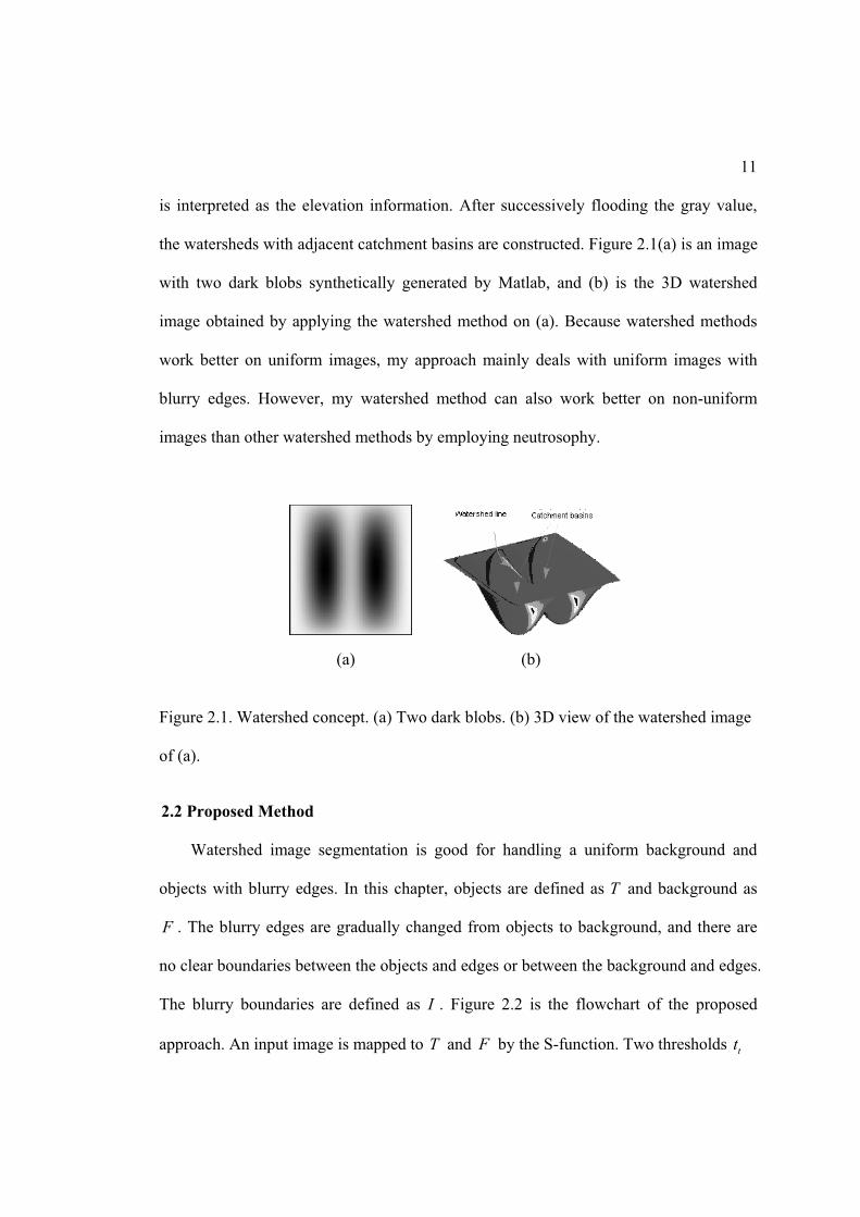
is interpreted as the elevation information. After successively flooding the gray value,

the watersheds with adjacent catchment basins are constructed. Figure 2.1(a) is an image

with two dark blobs synthetically generated by Matlab, and (b) is the 3D watershed

image obtained by applying the watershed method on (a). Because watershed methods

work better on uniform images, my approach mainly deals with uniform images with

blurry edges. However, my watershed method can also work better on non-uniform

images than other watershed methods by employing neutrosophy.

(a) (b)

Figure 2.1. Watershed concept. (a) Two dark blobs. (b) 3D view of the watershed image

of (a).

2.2 Proposed Method

Watershed image segmentation is good for handling a uniform background and

objects with blurry edges. In this chapter, objects are defined as T and background as

F . The blurry edges are gradually changed from objects to background, and there are

no clear boundaries between the objects and edges or between the background and edges.

The blurry boundaries are defined as I . Figure 2.2 is the flowchart of the proposed

approach. An input image is mapped to T and F by the S-function. Two thresholds tt

12

Figure 2.2. Flowchart of proposed method.

and ft are decided in the enhanced T and F domains. The original image is also mapped

to indeterminacy domain I . The boundary regions are calculated by combining ,T F and

I . The watershed method is applied to the boundary regions and finds connecting edges.

2.2.1 Map Image and Decide { , }T F

Given an image A , ( , )P x y is a pixel in the image, and ( ,x y ) is the position of this

pixel. A 5x5 mean filter (the size of filter may vary depending on the size of input image)

is applied to A to remove noise and make the image uniform. Next, the image is

converted by using the S-function:

2

2

0 0

( )( )( )

( , ) ( , , , )( )

1( )( )

1

xy

xyxy

xyxy

xy

xy

g a

g aa g b

b a c aT x y S g a b c

g cb g c

c b c ag c

(0.1)

Original image

S-function

Homogeneity

T, F

I

Enhancement thresholding

tt, tf

ThresholdO, E, B

Logic

Edge Watershed Segmentation

result

13

where xyg is the intensity value of pixel ( , )P i j . Variables ,a b and c are the parameters

that determine the shape of the S-function as shown in Figure 2.3.

Figure 2.3. S-function.

Values of parameters ,a b , and c can be calculated by using the simulated

annealing method [40]. However, the simulated annealing algorithm is quite time

consuming. Thus, we use another histogram-based method to calculate ,a b , and c [41].

(1) Calculate the histogram of the image

(2) Find the local maxima of the histogram: max 1 max 2 max( ), ( ), ... ( )nHis g His g His g .

Calculate the mean of local maxima:

max1

max

n

ii

His gHis g

n (0.2)

(3) Find the peaks greater than maxHis g , let the first peak be ming and the last peak be

maxg

(4) Define low limit 1B and high limit 2B :

14

1

min

max

2

1

1

( )

( )

B

i g

g

i B

His i f

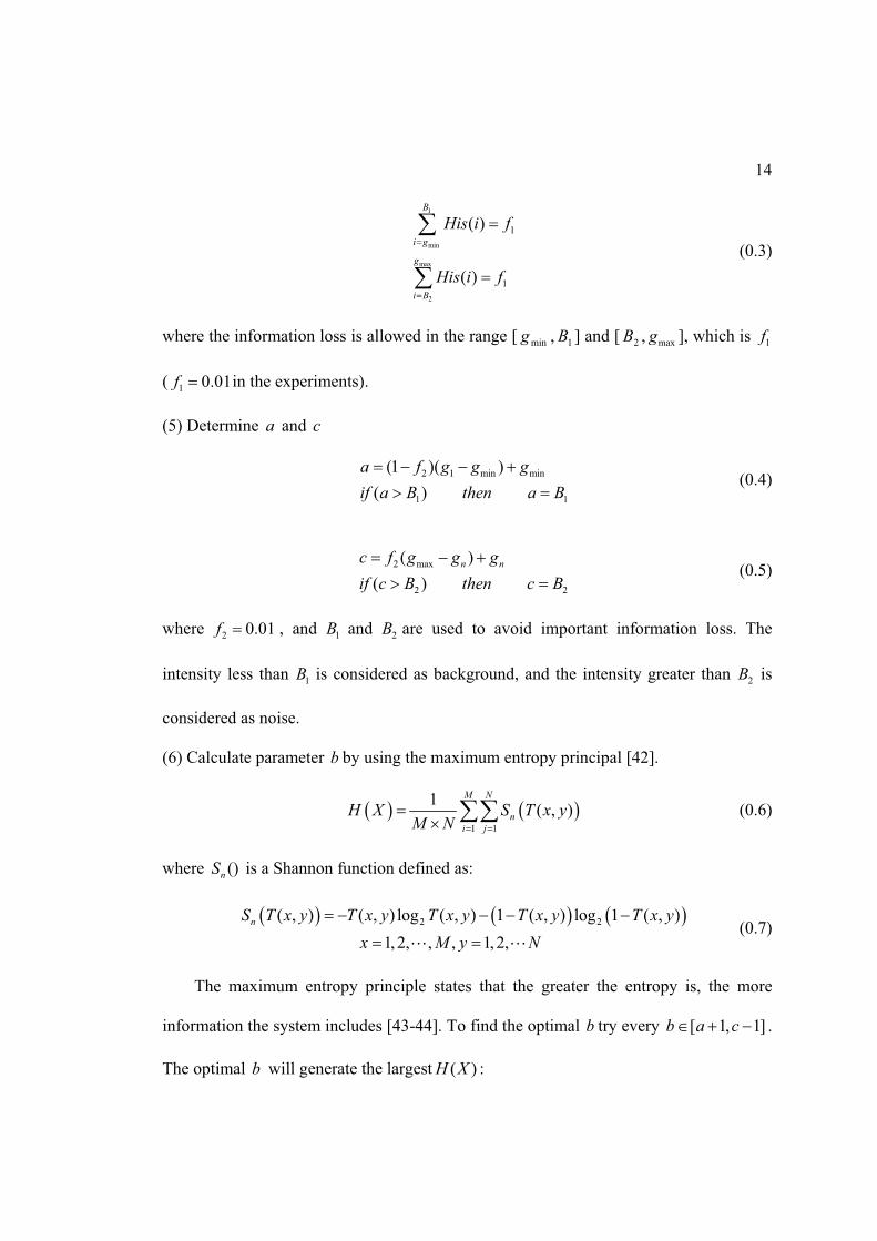
His i f (0.3)

where the information loss is allowed in the range [ ming , 1B ] and [ 2B , maxg ], which is 1f

( 1 0.01f in the experiments).

(5) Determine a and c

2 1 min min

1 1

(1 )( )( )

a f g g gif a B then a B

(0.4)

2 max

2 2

( )( )

n nc f g g gif c B then c B

(0.5)

where 2 0.01f , and 1B and 2B are used to avoid important information loss. The

intensity less than 1B is considered as background, and the intensity greater than 2B is

considered as noise.

(6) Calculate parameter b by using the maximum entropy principal [42].

1 1

1 ( , )M N

ni j

H X S T x yM N

(0.6)

where ()nS is a Shannon function defined as:

2 2( , ) ( , ) log ( , ) 1 ( , ) log 1 ( , )1, 2, , , 1, 2,

nS T x y T x y T x y T x y T x yx M y N

(0.7)

The maximum entropy principle states that the greater the entropy is, the more

information the system includes [43-44]. To find the optimal b try every [ 1, 1]b a c .

The optimal b will generate the largest ( )H X :

15

max min max, , , max ; , , |optH X a b c H X a b c g a b c g (0.8)

After ,a b , and c are determined, the image can be mapped from the intensity

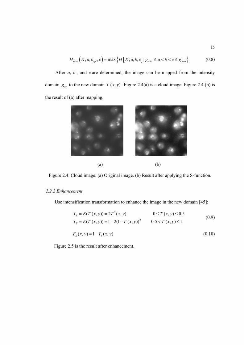
domain xyg to the new domain ( , )T x y . Figure 2.4(a) is a cloud image. Figure 2.4 (b) is

the result of (a) after mapping.

(a) (b)

Figure 2.4. Cloud image. (a) Original image. (b) Result after applying the S-function.

2.2.2 Enhancement

Use intensification transformation to enhance the image in the new domain [45]:

2

2

( ( , )) 2 ( , ) 0 ( , ) 0.5

( ( , )) 1 2(1 ( , )) 0.5 ( , ) 1E

E

T E T x y T x y T x yT E T x y T x y T x y

(0.9)

( , ) 1 ( , )E EF x y T x y (0.10)

Figure 2.5 is the result after enhancement.

16

Figure 2.5. Result after enhancement.

2.2.3 Find Thresholds in ET and EF

Two thresholds are needed to separate the new domains ET and EF . A heuristic

approach is used to find the thresholds in ET and EF [10].

(1) Select an initial threshold 0t in ET .

(2) Separate ET by using 0t , and produce two new groups of pixels: 1T and 2T , 1 and

2 are the mean values of these two parts, respectively.

(3) Compute the new threshold value: 1 21 2t

(4) Repeat steps 2 through 4 until the difference of 1n nt t is smaller than

( 0.0001 in the experiments) in the two successive iterations. Then, a threshold tt is

calculated. Figure 2.6(a) is the binary image generated by using tt .

Applying the above steps in EF domain, a threshold ft can be calculated. Figure

2.6(b) is the resulting image by using ft .

17

(a) (b)

Figure 2.6. Result after applying tt and ft . (a) Image by applying threshold tt . (b) Image by applying threshold ft .

2.2.4 Define Homogeneity and Decide I

Homogeneity is related to local information, and plays an important role in image

segmentation. I define homogeneity by using the standard deviation and discontinuity of

the intensity. Standard deviation describes the contrast within a local region, while

discontinuity represents the changes in gray levels. Objects and background are more

uniform, and blurry edges are gradually changing from objects to background. The

homogeneity value of objects and background is larger than that of the edges.

A size d d window centered at ( , )x y is used for computing the standard

deviation of pixel ( , )P i j :

( 1) / 2 ( 1) / 22

( 1) / 2 ( 1) / 22

( )( , )

x d y d

pq xyp x d q y d

gsd x y

d (0.11)

where xy is the mean of the intensity values within the window.

18

( 1) / 2 ( 1) / 2

( 1) / 2 ( 1) / 22

x d y d

pqp x d q y d

xy

g

d

The discontinuity of pixel ( , )P i j is described by the edge value. I use Sobel

operator to calculate the discontinuity.

2 2( , ) x yeg x y G G (0.12)

where xG and yG are the horizontal and vertical derivative approximations.

Normalize the standard deviation and discontinuity, and define the homogeneity as

max max

( , ) ( , )( , ) 1 sd x y eg x yH x ysd eg

(0.13)

where max max{ ( , )}sd sd x y , and max max{ ( , )}eg eg x y .

The indeterminate ( , )I x y is represented as

( , ) 1 ( , )I x y H x y (0.14)

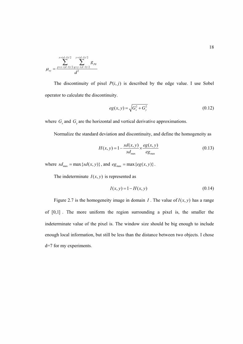
Figure 2.7 is the homogeneity image in domain I . The value of ( , )I x y has a range

of [0,1] . The more uniform the region surrounding a pixel is, the smaller the

indeterminate value of the pixel is. The window size should be big enough to include

enough local information, but still be less than the distance between two objects. I chose

d=7 for my experiments.

19

Figure 2.7. Homogeneity image in domain I .

2.2.5 Convert Image into Binary Image Based on { , , }E ET I F

In this step, a given image is divided into three parts: objects (O ), edges ( E ), and

background ( B ). ( , )T x y represents the degree of being an object pixel, ( , )I x y is the

degree of being an edge pixel, and ( , )F x y is the degree of being a background pixel for

pixel ( , )P x y , respectively. The three parts are defined as follows:

( , ) , ( , )( , )

( , ) ( , ) , ( , )( , )

( , ) , ( , )( , )

E t

E t E f

E f

true T x y t I x yO x y

false otherstrue T x y t F x y t I x y

E x yfalse others

true F x y t I x yB x y

false others

(0.15)

where tt and ft are the thresholds computed in Subsection 2.2.3, and 0.01.

After O , E , and B are determined, the image is mapped into a binary image for

further processing. The objects and background are mapped to 0, and the edges are

mapped to 1 in the binary image. The mapping function is as follows. See Figure 2.8.

0 ( , ) ( , ) ( , )( , )1

O x y B x y E x y trueBinary x yothers

(0.16)

20

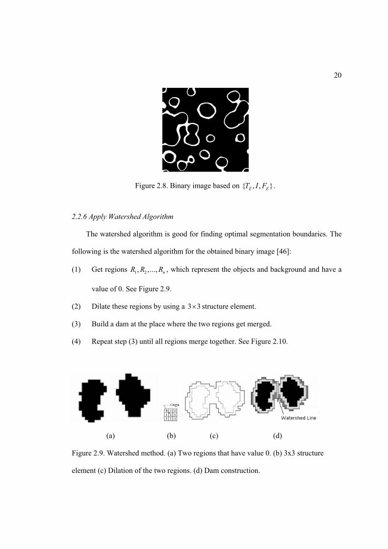
Figure 2.8. Binary image based on { , , }E ET I F .

2.2.6 Apply Watershed Algorithm

The watershed algorithm is good for finding optimal segmentation boundaries. The

following is the watershed algorithm for the obtained binary image [46]:

(1) Get regions 1 2, ,..., nR R R , which represent the objects and background and have a

value of 0. See Figure 2.9.

(2) Dilate these regions by using a 3 3 structure element.

(3) Build a dam at the place where the two regions get merged.

(4) Repeat step (3) until all regions merge together. See Figure 2.10.

(a) (b) (c) (d)

Figure 2.9. Watershed method. (a) Two regions that have value 0. (b) 3x3 structure

element (c) Dilation of the two regions. (d) Dam construction.

21

Figure 2.10. Final result after applying the proposed watershed method.

2.3 Experimental Results

Watershed segmentation is good for processing nearly uniform images; it can get a

good segmentation, and the edges are connected very well. But this method is sensitive

to noise and often has an over-segmentation problem [47]. I next compare my method

with the pixel-based, edge-based, region-based and other two watershed methods.

Figure 2.11(a) is a cloud image that has blurry boundaries, and (b) is the result by

using the pixel-based embedded confidence method [48], which determines the

threshold value of a gradient image and consequently performs edge detection. The

resulting image is under-segmented, and it only detects part of the boundaries. Figure

2.11(c) uses the Sobel operator which is an edge-based method. It, too, has under-

segmentation, and the boundaries are not connected well. Figure 2.11(d) is the result by

using the edge detection and image segmentation system (EDISON) [49] which applies

a mean-shift region-based method [50]. In mean-shift-based segmentation, pixel clusters

or image segments are identified with unique modes of the multi-modal probability

density function by mapping each pixel to a mode using a convergent, iterative process.

Three parameters in EDISON need to be manually selected: spatial bandwidth, color,

22

(a) (b) (c)

(d) (e) (f)

(g)

Figure 2.11. Cloud image. (a) Original image. (b) Result using the embedded confidence method. (c) Result using the Sobel operator. (d) Result using the mean-shift method. (e) Result using the watershed in Matlab. (f) Result using toboggan-based watershed. (g) Result using the proposed method.

23

and minimum region. I tried different combinations of these parameters and got the best

result, as shown in Figure 2.11(d) (spatial bandwidth = 6, color = 3, minimum = 50).

The edges in (d) are well connected but not smooth, the result is over-segmented. Figure

2.11(e) utilizes the watershed method in Matlab, and the result shows heavy over-

segmentation, making it hard to find distinguishable objects. Figure 2.11(f) is the result

from a modified watershed method (toboggan-based method) [51]. It can efficiently

group the local minima by assigning them a unique label. The result is better than (e),

but the background and objects are still mixed together. Figure 2.11(g) applies the

proposed method, and it gets clear and well connected boundaries. The result gives an

improvement better than those obtained by other methods used in (b), (c), (d), (e), and

(f).

Figure 2.12(a) is a blurry cells image. The objects and boundaries are not clear. The

edges detected by the embedded confidence method in (b) are discontinued. The Sobel

operator in (c) almost loses all boundaries. The mean-shift method in (d) (spatial

bandwidth= 7, color = 3, minimum = 10) produces few connected edges, and the edges

are not well detected. Two watershed methods in (e) and (f) produce over-segmentation.

The result in (g) using the proposed method has well connected and clear boundaries to

segment the cells from the background better.

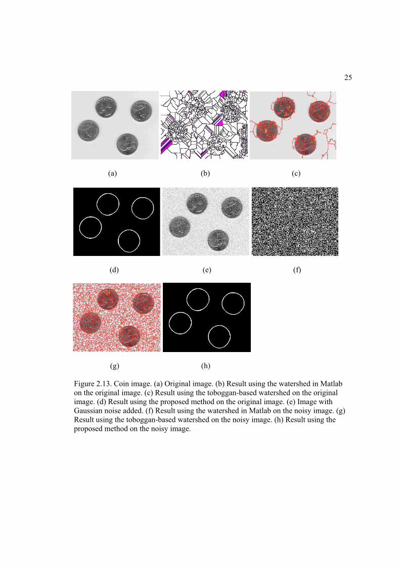
One drawback of watershed methods is noise sensitivity. However, the proposed

method is very noise-tolerant. Figure 2.13(a) is a noise-free coin image, and (b), (c), and

(d) are the results from employing the watershed method in Matlab, toboggan-based

watershed method, and the proposed neutrosophic watershed method, respectively.

24

(a) (b) (c)

(d) (e) (f)

(g)

Figure 2.12. Cell image. (a) Blurry cell image. (b) Result using the embedded confidence edge detector. (c) Result using the Sobel operator. (d) Result using the mean-shift method. (e) Result using the watershed in Matlab. (f) Result using the toboggan-based watershed. (g) Result using the proposed method.

25

(a) (b) (c)

(d) (e) (f)

(g) (h)

Figure 2.13. Coin image. (a) Original image. (b) Result using the watershed in Matlab on the original image. (c) Result using the toboggan-based watershed on the original image. (d) Result using the proposed method on the original image. (e) Image with Gaussian noise added. (f) Result using the watershed in Matlab on the noisy image. (g) Result using the toboggan-based watershed on the noisy image. (h) Result using the proposed method on the noisy image.

26

Figure 2.13(e) is the image after adding Gaussian noise (mean is 0, and standard

variance is 2.55) to (a). Figure 2.13(f), (g), and (h) are the results from applying the

above three watershed methods to (e). We can see that the Gaussian noise has a big

impact on the results of the existing watershed methods, and causes heavy over-

segmentation. But the proposed neutrosophic watershed method is quite noise-tolerant.

Another problem of existing watershed algorithms is that they do not work well for

non-uniform images. In Figure 2.14(a), the capitol has a wide range of intensities. The

top of the capitol is dark, the middle part of the capitol is gray, and the bottom part of

capitol is white. Figure 2.14(b) is the result of applying the watershed method in Matlab,

and (c) is the result of applying the toboggan-based watershed method. Neither works

well. Figure 2.14(d) is the result of applying the proposed method. As shown, the capitol

is segmented well.

2.4 Conclusions

In this chapter, neutrosophy is employed in gray level images, and a novel

watershed image segmentation approach based on neutrosophic logic is introduced. In

the first phase, a given image is mapped to three subsets ,T F and I , which are defined

in different domains. Thresholding and neutrosophic logic are employed to obtain a

binary image. Finally, the proposed watershed method is applied to get the segmentation

result. I compare my method with pixel-based, edge-based, region-based segmentation

methods, and two existing watershed methods. The experiments show that the proposed

method has better performance on noisy and non-uniform images than that obtained by

27

using other watershed methods, since the proposed approach can handle uncertainty and

indeterminacy better.

28

(a) (b)

(c) (d)

Figure 2.14. Capitol image. (a) Original capitol image. (b) Result using the watershed in Matlab. (c) Result using the toboggan-based method. (d) Result using the proposed method.

29

CHAPTER 3

BREAST ULTRASOUND IMAGE SEGMENTATION

BASED ON NEUTROSOPHY

3.1 Introduction

Cancer is one of the dangerous diseases for humans. One out of eight deaths in the

world is caused by cancer [52]. It is the second leading cause of death in developed

countries and the third leading cause of death in developing countries. According to [53],

in 2009, 562,340 Americans, 1,500 people a day, died of cancer. Approximately

1,479,350 new cancer cases were diagnosed in the United States in 2009.

Breast cancer is the most commonly diagnosed cancer among women and is the

second leading death cause of women in the United States [54]. A total 209,060 new

breast cancer cases and 40,230 deaths are projected to occur in 2010 [55]. Although

breast cancer has a high death rate, the cause of breast cancer is still unknown [56].

Early detection is a critical step towards treating breast cancer and plays a key role in

diagnosis.

There are three major types of diagnostic techniques used by radiologists to detect

breast cancer: mammography [57-58], ultrasound, and magnetic resonance imaging

(MRI).

While mammography is the most frequently used of these techniques, it has some

disadvantages:

1. It is not always accurate in detecting breast cancer [59]. Approximately 65% of

cases referred to surgical biopsy are actually benign lesions [60-61].

30

2. Mammography has limitations in cancer detection in the dense breast tissue of

young patients. The breast tissue of young women tends to be dense and full of

milk glands. Most cancers arise in dense tissue, and it is challenging for

mammography to detect lesion in this higher risk category.

3. In mammograms, glandular tissues look dense and white, much like cancerous

tumors [62].

4. Mammography may identify an abnormality that looks like a cancer, but turns

out to be normal. Thus, additional tests and diagnostic procedures are often

required. It is a stressful procedure for patients. To make up for these

limitations, sound diagnosis is often needed in addition to mammography [63].

5. Reading mammograms is a demanding job for radiologists. An accurate

diagnosis depends on training, experience, and other subjective criteria.

Around 10 percent of breast cancers are missed by radiologists, and most of

them are in dense breasts [64]. And about two-thirds of the lesions that are sent

for biopsy are benign. The reasons for this high miss rate and low specificity in

mammography are the following: the low conspicuity of mammographic

lesions, the noisy nature of the images, and the overlying and underlying

structures that obscure features of a region of interest (ROI) [65].

Ultrasound techniques use high frequency broadband sound waves in the megahertz

range. These waves are reflected by tissue to varying degrees to produce images. An

ultrasound image is a gray level display of the area being imaged and is used in imaging

abdominal organs, heart, breast, muscles, tendons, arteries and veins. An ultrasound

31

allows for studying the function of moving structures in real-time and has no ionizing

radiation. It is relatively cheap and quick to perform. Since an ultrasound is noninvasive,

practically harmless, and cost effective for diagnosis, it has become one of the most

prevalent and effective medical imaging technologies. In breast cancer detection, it is an

important adjunct to mammography and has following advantages:

1. Use of ultrasounds in breast cancer detection has improved the true positive

detection rate, especially for women with dense breasts [66-67]. According to

[68], an ultrasound is more effective for women younger than 35. It has

proven to be an important adjunct to mammography in breast cancer detection

and useful for differentiating cysts from solid tumors.

2. It has been shown that ultrasound is superior to mammography in its ability to

detect local abnormalities in the dense breasts of adolescent women [69]. The

authors of [70] suggest that the denser the breast parenchyma, the higher the

detection accuracy of malignant tumors using ultrasound. The accuracy rate of

breast ultrasound (BUS) has been reported to be 96-100% in the diagnosis of

simple benign cysts [71].

3. An ultrasound can obtain any section image of breast, and observe the breast

tissues in real-time and dynamically.

4. Ultrasound devices are portable and relatively cheap, and they have no

radiation and side effects.

However, ultrasound imaging has some limitations. It is low contrast, low

resolution with speckle noise and blurry edges between different organs. These

32

characteristics make it is more difficult for radiologists to read and interpret ultrasound

images. Table 3.1 lists the accuracy rate of doctors.

Table 3.1. Accuracy Rate of BUS Examination.

Type Accuracy

Benign hyperplasia 84.5%

Benign tumor 79%

Malignant tumor 88.5%

Computer-aided detection (CAD) systems have been developed to help radiologists

to evaluate medical images and detect lesions at an early stage [72]. They assist doctors

in the interpretation of medical images. A typical CAD system in breast ultrasound helps

radiologists evaluate ultrasound images and detect breast cancer. A breast ultrasound

CAD system improves the ultrasound image quality, increases the image contrast, and

automatically determines lesion. It also reduces the human workload. Figure 3.1 gives

the general steps of an ultrasound CAD system.

Figure 3.1. Breast ultrasound CAD system.

Image Preprocessing

Image Segmentation

Input Image

33

Breast ultrasound (BUS) images are low contrast and have speckles, thus making

the segmentation of BUS images one of the most difficult steps in computer-aided

diagnosis (CAD) algorithms. There is a controversy between two opinions about speckle

in BUS images. (1) Speckle blurs a BUS image, and it is treated as noise to be removed

[73-74]. (2) Speckle reflects the local echogenity of the underlying scatters and has

certain useful pattern elements [75]. Most of the existing CAD systems are based on one

of the above two opinions about speckle. Another problem in most of the existing BUS

segmentation methods is that the algorithms are only applied to a restricted area, a

region of interest (ROI), rather than the entire BUS image. The ROIs contain tumors

[76-77], and they are manually or semi-automatically segmented [78]. There are four

types of methods used for BUS image segmentation: edge-based methods [79-80],

region-based methods [81-82], model-based methods [83], and neural network/Markov

methods [84-86].

A BUS image is noisy and blurry due to artifacts, such as speckle, reverberation

echo, acoustic shadowing, and refraction [87]. The boundaries of the tumors are unclear

and hard to distinguish. In this paper, I define a tumor as <A>, the boundaries of the

tumor as <Neut-A>, and the background as <Anti-A>. ,T I , and F are the neutrosophic

components to represent <A>, <Neut-A>, and <Anti-A>. <A> and <Anti-A> contain

region information, while <Neut-A> has boundary information.

A pixel of an image in the neutrosophic domain can be represented as { , , }A t i f ,

meaning the pixel is %t true (tumor), %i indeterminate (tumor boundaries), and %f

false (background), where t T , i I ,and f F , and T, I and F represent true,

34

indeterminacy and false domains, respectively. In the classical set, 0i , t and f are

either 0 or 100. In the fuzzy set, 0i , 0 , 100t f . In the neutrosophic set,

0 , , 100t i f .

3.2 Tumor Detection Method

Because a BUS is blurred image, I can use the algorithm presented in Chapter 2 to

find the boundaries of a tumor. However, because BUS images contain speckles,

reverberation echoes, and acoustic shadow artifacts, the segmentation result may include

non-tumor area. I remove such areas by utilizing the following rules:

(1) Remove the lines connected to the image boundaries.

(2) Remove the segmentation area whose size is less than one-third of the largest

segmented area.

(3) Remove the segmentation area whose mean gray level is greater than the average

gray level of the entire image.

(4) Remove the area whose ratio of width/length is equal to or greater than 4, since

the shape of the tumor should be roundish or elliptical.

Figure 3.2 is the flowchart of BUS detection based on neutrosophy. Since the

watershed method shrinks the segmented area, I use the boundary produced in

Subsection 2.2.5 as the tumor boundary. Figure 3.3 is the resulting images of each step.

35

Figure 3.2. Flowchart of BUS detection.

(a) (b)

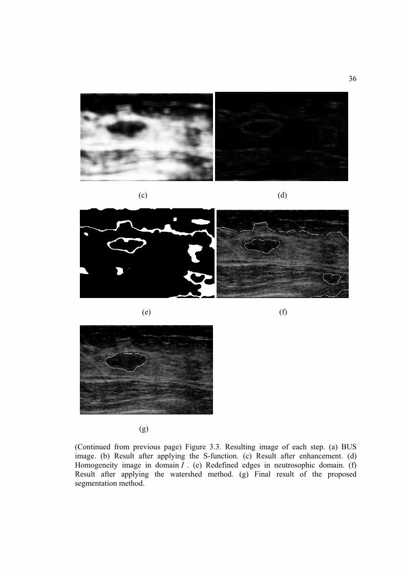
Figure 3.3. Resulting image of each step. (Continued on next page)

Original image

S-function

Homogeneity

T, F

I

Enhance and thresholding

tt, tf

Threshold O, E, B

Logic

Edge Boundaries Watershed Locate tumor Segmentation

result

36

(c) (d)

(e) (f)

(g)

(Continued from previous page) Figure 3.3. Resulting image of each step. (a) BUS image. (b) Result after applying the S-function. (c) Result after enhancement. (d) Homogeneity image in domain I . (e) Redefined edges in neutrosophic domain. (f) Result after applying the watershed method. (g) Final result of the proposed segmentation method.

37

3.3 Experimental Results

My approach has the following advantages: it is noise-tolerant, fully automatic, and

able to process low-contrast BUS images with high accuracy. The database used in my

experiments contains 110 images (53 malignant, 37 benign, and 20 normal). Each image

has only one tumor. The average size of image in the database is 370x450 pixels, with

the largest being 470x560 pixels and the smallest 260x330 pixels. The images were

collected by VIVID 7 with a 5-14 MHz linear probe. I used 10 images (5 malignant and

5 benign), in which were included the largest and smallest tumors, to determine the

parameters of the algorithm.

3.3.1 Speckle Problem

As stated previously, there are two controversial opinions about speckle in BUS

images: speckle is noise versus speckle is pattern. My method solves this controversy by

combining these two opinions through use of neutrosophy. In T or F , the speckle is

treated as noise. In I , the speckle is employed as a pattern for computing homogeneity.

In Chapter 2, I demonstrate the noise-tolerance of the proposed algorithm in Figure 2.13

by adding Gaussian noise to (a).

3.3.2 Fully Automatic Method

One of the more difficult problems in BUS image segmentation is to find the tumor

automatically. Many existing methods need to manually select a region containing the

tumor as the initialization of segmentation. Often, the final segmentation depends on

region selection. The geodesic active contour (GAC) model is an edge-based model [88].

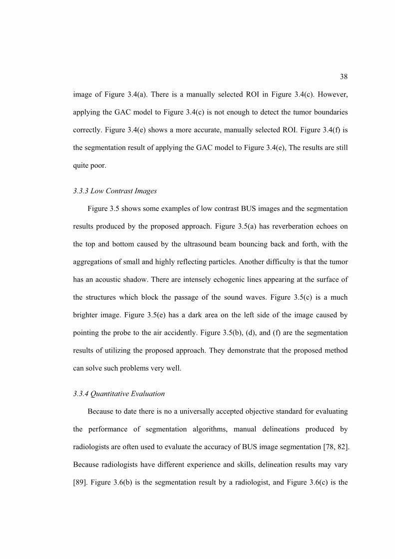
Figure 3.4(b) is the segmentation result by applying the GAC model to the entire BUS

38

image of Figure 3.4(a). There is a manually selected ROI in Figure 3.4(c). However,

applying the GAC model to Figure 3.4(c) is not enough to detect the tumor boundaries

correctly. Figure 3.4(e) shows a more accurate, manually selected ROI. Figure 3.4(f) is

the segmentation result of applying the GAC model to Figure 3.4(e), The results are still

quite poor.

3.3.3 Low Contrast Images

Figure 3.5 shows some examples of low contrast BUS images and the segmentation

results produced by the proposed approach. Figure 3.5(a) has reverberation echoes on

the top and bottom caused by the ultrasound beam bouncing back and forth, with the

aggregations of small and highly reflecting particles. Another difficulty is that the tumor

has an acoustic shadow. There are intensely echogenic lines appearing at the surface of

the structures which block the passage of the sound waves. Figure 3.5(c) is a much

brighter image. Figure 3.5(e) has a dark area on the left side of the image caused by

pointing the probe to the air accidently. Figure 3.5(b), (d), and (f) are the segmentation

results of utilizing the proposed approach. They demonstrate that the proposed method

can solve such problems very well.

3.3.4 Quantitative Evaluation

Because to date there is no a universally accepted objective standard for evaluating

the performance of segmentation algorithms, manual delineations produced by

radiologists are often used to evaluate the accuracy of BUS image segmentation [78, 82].

Because radiologists have different experience and skills, delineation results may vary

[89]. Figure 3.6(b) is the segmentation result by a radiologist, and Figure 3.6(c) is the

39

result generated after the discussion of a group of radiologists. Figure 3.6(d) is the result

by using the proposed approach.

Figure 3.7(a), (c) and (e) are the manual segmentation results by a group of

radiologists. Figure 3.7(b), (d) and (e) are the results by the proposed algorithm. We can

see that the proposed approach can outline the tumor shape very well, which is one of

the most important features for CAD systems [90].

An active contour (AC) model is a region-based segmentation method [91-93]. It

utilizes the means of different regions to segment a BUS image. Because AC requires

manually selecting an ROI, I use a rectangular ROI that contains a tumor. The length

and width of an ROI region are 2 times the length and width of the tumor. Figure 3.8(b)

is the result by applying an AC model with 200 iterations to Figure 3.8(a). The result

shows over-segmentation. Figure 3.8(c) is the result after removing the non-tumor

region. However, the AC model does not work well on some BUS images (see Figure

3.8(e)).

In their recently published paper, the authors of [94] employ a fully automatic

segmentation method on BUS images based on texture analysis and active contour (TE).

It first divides the entire image into lattices of the same size, and then generates the ROI

based on the texture information. Figure 3.9(b) is the result of applying the method in

[94]. But this method will not work well on low contrast images (reverberation echoes,

refraction, etc). Figure 3.9(d) segments a part of the background as a part of the tumor.

Figure 3.9(f) locates the wrong ROI region.

40

(a) (b)

(c) (d)

(e) (f)

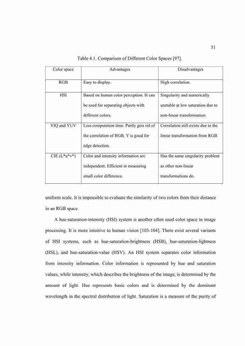
Figure 3.4. Result of GAC method. (a) BUS image. (b) The segmentation result by applying GAC model to (a). (c) Manually selected ROI. (d) The segmentation result by applying GAC Model to (c). (e) More accurately and manually selected ROI. (f) The segmentation result by applying GAC Model to (e).

41

(a) (b)

(c) (d)

(e) (f)

Figure 3.5. Low quality images. (a) BUS image with reverberation echo and shadow. (b) Result using the proposed method. (c) Bright BUS image. (d) Result using the proposed method. (e) BUS image with dark area on the left side. (f) Result using the proposed method.

Shadows

Reverberation echoes

42

(a) (b)

(c) (d)

Figure 3.6. Comparison with manual outlines. (a) BUS image. (b) Manual segmentation result by a radiologist. (c) Manual segmentation result by a group of radiologists. (d) Result by using the proposed method.

43

(a) (b)

(c) (d)

(e) (f)

Figure 3.7. Result of proposed method. (a), (c) and (e) Manual segmentation results by a group of radiologists. (b), (d), and (f) Results by using the proposed algorithm.

44

(a) (b) (c)

(d) (e)

Figure 3.8. Result of AC method. (a) BUS images with manually selected ROI. (b) Results by applying active contour method. (c) Result by removing non-tumor areas. (d) BUS images with manually selected ROI. (e) Results by applying active contour method.

45

(a) (b)

(c) (d)

(e) (f)

Figure 3.9. Result of TE method. (a), (c) and (e) BUS images. (b), (d) and (e) Result by applying the TE method in [95].

46

In this paper, I tested my method using 90 clinical images and used three area

error metrics [96] for evaluating accuracy: true positive ratio (TP), false positive ratio

(FP), and similarity (SI) defined as:

(%)

(%)

(%)

m n

m

m n n

m

m n

m n

A ATP

AA A A

FPA

A ASI

A A

(1.1)

where mA refers to the tumor area determined by a group of radiologists and nA is the

area determined by the proposed algorithm, see Figure 3.10.

Figure 3.10. Areas corresponding to TP, FP, and FN.

In Table 3.2, active contour (AC) method, texture-based method (TE), and the

proposed method are compared with the delineated results by the group of radiologists.

Manual Drawing Computer Drawing

True Positive

False Negative

False Positive

47

Table 3.2. Average Area Error Metrics.

Malignant Benign Total

TP FP Similarity TP FP Similarity TP FP Similarity

AC1 64.1% 5.3% 63.7% 71.5% 6.8% 66.8% 67.4% 5.98% 65.1%

TE2 81.2% 38.3% 51.1% 84.2% 44.5% 47.8% 82.9% 41.2% 49.1%

Proposed

method3

85.4% 11.7% 77.6% 89.6% 14.3% 78.3% 87.8% 13.3% 77.9%

1 The inputs of active contour method are the manually selected ROIs. There are 40 out of 90 images in which the tumors can be located. 2 The inputs of texture-based method are the entire BUS images. There are 62 out of 90 images in which the tumors can be located. 3 The inputs of proposed method are entire BUS images. There are 84 out of 90 images in which the tumors can be located.

The source code of active contour is obtained from an introduction website of the

AC method, which is based on [91]. It includes the application to medical image

segmentation. In an active contour method, the input is a manually selected ROI. There

are only 40 results for locating a tumor properly (90 images in the database). The

accuracy of AC is calculated based on these 40 images. We can see that the TP (67.4%

in total) of the AC method is very low even using ROIs only.

The inputs of TE and the proposed method are the entire BUS images, because both

of them are designed as fully automatic methods. TE has 62 results correctly locating the

tumors and the proposed method has 84. But, the false positive rate of TE is 41.2%

which is too high to be useful. The proposed method has high similarity (77.9% in total).

The mean shortest distance error, standard deviation, and maximum value between

these three algorithms’ contours and doctors’ manual contours are listed in Table 3.3.

The proposed method has the smaller shortest distance error (6.9 pixels), standard

deviation (3.9 pixels), and maximum value (16.1 pixels). Figure 3.11 is TP versus FP

48

plotting Figure, which was used in clinical data analysis [77]. The proposed method

yields estimate in the upper left corner of ROC which provided high sensitivity and

specificity than other two methods.

Table 3.3. Shortest Distance Comparison among Three Algorithms.

AC TE Proposed method Mean shortest distance 24.8 pixels 41.7 pixels 6.9 pixels Standard Deviation 17 pixels 29 pixels 3.9 pixels

Maximum Value 76.9 pixels 92.7 pixels 16.1 pixels

Another problem in BUS segmentation is handling non-tumor images. A TE

method does not work for non-tumor BUS images. It always returns a tumor area. I

tested the proposed method with 20 non-tumor images; 15 of them got correct results.

Because the proposed algorithm does not use an iterative method to determine the

boundaries, the computation time is much less than that of the other two methods. The

computational times for active contour methods, texture-based methods, and the

proposed method are 65 seconds, 62 seconds, and 4 seconds, respectively. The

experiments used BUS images of the size 450x400, Matlab 2008, Pentium D 3.00GHZ,

and 3GB RAM.

3.4 Conclusions

In this chapter, neutrosophy is employed in BUS image segmentation. It integrates

the two controversial opinions about speckles: speckles are noise versus speckles

include pattern information. The proposed method is fully automatic, effective, and

49

robust. It can segment entire BUS images without manual initialization. The method is

also faster than other methods. The experiment results show that the proposed method

can segment low contrast BUS images with high accuracy.

(a) (b)

(c)

Figure 3.11. TP versus FP plotting. (a) Plotting of activate contour method. (b) Plotting of TE method. (c) Plotting of proposed method.

50

CHAPTER 4

COLOR IMAGE SEGMENTATION

BASED ON NEUTROSOPHY

4.1 Introduction

Color images contain more information than do gray level images, and they are

more close to the real-world [97-98]. The human eye can distinguish thousands of color

shades and intensities but only two-dozen shades of gray. Quite often, objects that

cannot be extracted using a gray scale can be extracted using color information.

Relatively inexpensive color cameras are nowadays available. In digital image libraries,

large collections of images and videos are color. They need to be catalogued, ordered,

and stored for efficient browsing and retrieval of visual information [99-100]. Although

color information permits a more complete representation of images, processing color

images requires more computation time than that needed for gray level images.

Unlike gray level images, several color spaces exist for representing a color image,

such as RGB, HIS, YIQ, YUV, and CIE. Table 4.1 lists the advantages and

disadvantages of these color spaces.

RGB is the most commonly used model in television systems and digital cameras.

While RGB is suitable for color display, it is not good for color scene segmentation and

analysis due to the high correlation among the R, G, and B [101-102]. High correlation

means that if the intensity changes, all the three components will change accordingly.

The measurement of a color in RGB space does not represent color differences in a

51

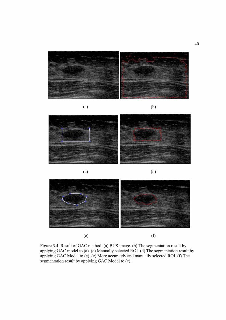
Table 4.1. Comparison of Different Color Spaces [97].

Color space Advantages Disadvantages

RGB Easy to display. High correlation.

HSI Based on human color perception. H can

be used for separating objects with

different colors.

Singularity and numerically

unstable at low saturation due to

non-linear transformation.

YIQ and YUV Less computation time. Partly gets rid of

the correlation of RGB. Y is good for

edge detection.

Correlation still exists due to the

linear transformation from RGB.

CIE (L*u*v*) Color and intensity information are

independent. Efficient in measuring

small color difference.

Has the same singularity problem

as other non-linear

transformations do.

uniform scale. It is impossible to evaluate the similarity of two colors from their distance

in an RGB space.

A hue-saturation-intensity (HSI) system is another often used color space in image

processing. It is more intuitive to human vision [103-104]. There exist several variants

of HSI systems, such as hue-saturation-brightness (HSB), hue-saturation-lightness

(HSL), and hue-saturation-value (HSV). An HSI system separates color information

from intensity information. Color information is represented by hue and saturation

values, while intensity, which describes the brightness of the image, is determined by the

amount of light. Hue represents basic colors and is determined by the dominant

wavelength in the spectral distribution of light. Saturation is a measure of the purity of

52

color and signifies the amount of white light mixed with the hue. Figure 4.1 is a

geometrical description of HSI [105]. Hue is considered as an angle between a reference

line and the color point in RGB space with the range value from 0o to 360o. For example,

green is 120o and blue is 240o. The saturation component represents the radial distance

from the cylinder center. The nearer the point is to the center, the lighter the color.

Intensity is the height in the axis direction. For example, 0 intensity is black, full

intensity is white. Each slice of the cylinder has the same intensity. Because human

vision system can easily distinguish the difference of hue, HSI has a good ability to

represent the human color perception. The following formulas transfer RGB to HSI:

3( )arctan( ) ( )

( )3

min( , , )1

G BHR G R B

R G BInt

R G BSatl

Figure 4.1 HSI color space [105].

53

YIQ is used to encode color information in TV signals in the American system. Y is

a measure of the luminance of the color, and is a possible candidate for edge detection. I

and Q are components jointly describing image hue and saturation [106]. The YIQ color

space can partly get rid of the correlation of RGB color space, and the linear

transformation needs less computation time than the nonlinear transformation. YIQ is

obtained from the RGB by a linear transformation:

0.299 0.587 0.1140.596 0.274 0.3220.211 0.253 0.312

X RY GZ B

where 0 1,0 1,0 1R G B .

YUV is another TV color representation and is used in the European TV system.

The transformation formula is:

0.299 0.587 0.1140.147 0.289 0.437

0.615 0.515 0.100

X RY GZ B

where 0 1,0 1,0 1R G B .

The Commission International de l’Eclairage (CIE) color space was created to

represent perceptual uniformity. It meets the psychophysical need for a human observer.

Three primaries in CIE is denoted as ,X Y , and Z . Any color can be specified by the

combination of ,X Y , and Z . The value of ,X Y , and Z can be computed by a linear

transformation from RGB. Here is an example of the National Television System

Commission, United States (NTSC) transformation matrix:

54

0.607 0.174 0.2000.299 0.587 0.1140.000 0.066 1.116

X RY GZ B

There are a number of CIE spaces that can be created if the XYZ tristimulus

coordinates are known. For example, CIE(L*a*b*) and CIE(L*u*v*) are two typical

CIE spaces. The definition of CIE(L*a*b*) is:

3

0

3 3

0 0

3 3

0 0

* 116 ( ) 16

* 500

* 500

YLY

X YaX Y

Y ZbY Z

where 0 0/ 0.01, / 0.01Y Y X X , and 0/ 0.01Z Z . 0 0 0, , X Y Z are , , X Y Z values

for the standard white. The definition of CIE(L*u*v*) is given in the next section. The

difference of two colors in these two spaces can be calculated as the Euclidean distance

between two color points like this: 2 2 2( *) ( *) ( *)abE L a b or

2 2 2( *) ( *) ( *)abE L u v . Euclidean distance has the ability to express the

color difference of human perception. (L*a*b*) and (L*u*v*) are approximately a

uniform chromaticity scale, which matches the sensitivity of human eyes in computer

processing [107], whereas RGB and XYZ color space do not have such properties. HSI

can be mapped to the cylindrical coordinates of (L*a*b*) or (L*u*v*) space by these:

55

2 2

( * * *)*

arctan( * / *)

( *) ( *)

HSI to CIE L a bI LH a b

S a b

and

2 2

( * * *)*

arctan( * / *)

( *) ( *)

HSI to CIE L u vI LH u v

S u v

(L*a*b*) and (L*u*v*) share the same L* value, which defines the lightness, or

the intensity of a color. CIE spaces can control color and intensity information more

independently and simply than RGB space. Direct color comparison can be performed

based on geometric separation within the color space. Therefore, CIE space is especially

efficient in measuring small color differences.

Most color image segmentation methods are based on gray level image

segmentation approaches with different color representations. The authors of [97, 108]

mention that color images can be considered as a special case of multi-spectral images,

and any segmentation method for multi-spectral images can be applied to color images,

see Figure 4.2 [97]. Most gray level segmentation techniques can be extended to color

images, such as histogram thresholding, clustering, region growing, edge detection, etc.

Gray level segmentation methods can be directly applied to each component of a color

space. The results next are combined in some way to get the final segmentation result

[109]. But there exist two problems:

56

Figure 4.2 Relationship between gray level segmentation and color segmentation.

1. When the color is projected onto three components, the color information is

scattered such that the color image becomes simply a multispectral image and the

color information that humans can perceive is lost.

2. Each color representation has its advantages and disadvantages. There is no

single color representation than surpasses others for segmenting all kinds of

color images.

Most of existing color image segmentation methods define a region based on similarity of

color. This assumption often makes it difficult for algorithms to separate the objects with

highlights, shadows, shadings, or texture. This causes inhomogeneity of colors. Most

color segmentation methods are only conducted in one color space [97, 110-111]. Color

segmentation techniques can be grouped into several categories: histogram methods,

space clustering methods, edge-based methods, region-based methods, neural network

Gray level segmentation Methods

Histogram-based Space Clustering Edge-based Region-based Neural Network Fuzzy Logic

Color Segmentation Methods

Color Spaces RGBHSIYIQ YUV

CIE(L*a*b*) CIE(L*u*v*)

57

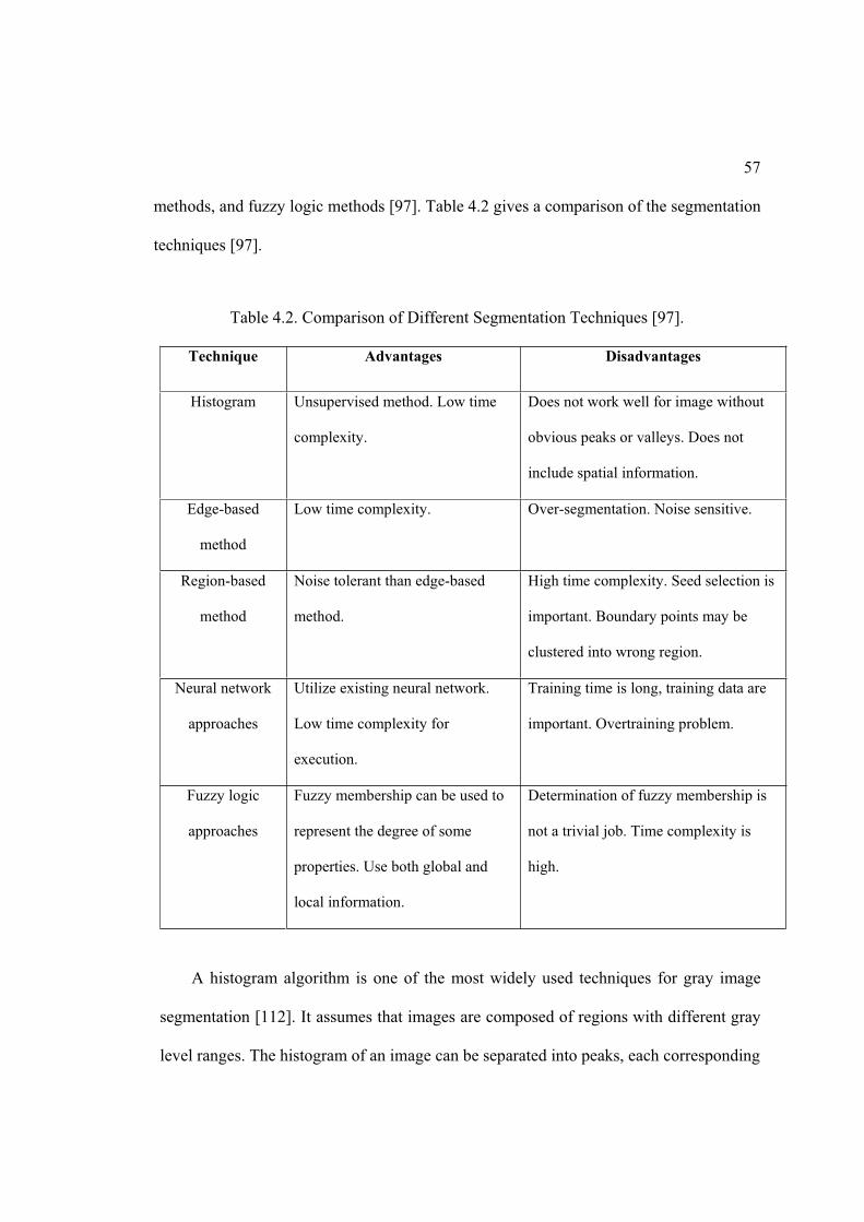
methods, and fuzzy logic methods [97]. Table 4.2 gives a comparison of the segmentation

techniques [97].

Table 4.2. Comparison of Different Segmentation Techniques [97].

Technique Advantages Disadvantages

Histogram Unsupervised method. Low time

complexity.

Does not work well for image without

obvious peaks or valleys. Does not

include spatial information.

Edge-based

method

Low time complexity. Over-segmentation. Noise sensitive.

Region-based

method

Noise tolerant than edge-based

method.

High time complexity. Seed selection is

important. Boundary points may be

clustered into wrong region.

Neural network

approaches

Utilize existing neural network.

Low time complexity for

execution.

Training time is long, training data are

important. Overtraining problem.

Fuzzy logic

approaches

Fuzzy membership can be used to

represent the degree of some

properties. Use both global and

local information.

Determination of fuzzy membership is

not a trivial job. Time complexity is

high.

A histogram algorithm is one of the most widely used techniques for gray image

segmentation [112]. It assumes that images are composed of regions with different gray

level ranges. The histogram of an image can be separated into peaks, each corresponding

58

to one region. There is a threshold value for separating two adjacent peaks. In color

images, the situation is different from a gray image because of multi-features. Multiple

histogram-based thresholding divides a color space by thresholding each component

histogram. There is a limitation when dividing multiple dimensions, however, because

thresholding is a technique for gray scale images. In many approaches, thresholding is

performed on only one color component at a time. Thus, the regions extracted are not

based on the information available from all three components simultaneously. The

correlation among the three components is neglected.

Edge-based techniques are extensively utilized in gray level image segmentation.

They are based on the detection of discontinuity and locating points with abrupt changes

in gray level. Edge-based methods are usually classified into two categories: sequential

and parallel [113]. In color images, the information about edges is much richer than that

in gray images. For example, edges between two objects with the same brightness but

different hue can be detected in color images [114]. Accordingly, in a color image, an

edge should be defined by a discontinuity in a three-dimensional color space. There are

three alternatives for the definition of a color edge:

1. Define a metric distance in some color space, and use discontinuities in the

distance to determine edges [115].

2. Regard a color image as composed of three gray images formed by the three

color components, respectively. Perform gray level edge detection on these three

images separately. Then, the edges detected in the three images are merged by

specified procedures [116-117].

59

3. Impose some uniformity constraints on the edges in the three color components

to utilize all of the three color components simultaneously, but allow the edges in

the three color components to be largely independent [115].

Region-based techniques include region growing, region splitting, region merging,

and their combination. In the region growing approach, seed regions are first selected,

then expanded to include all homogeneous neighbors. This process is repeated until all

pixels in the image are classified. One problem with region growing is its dependence on

the selection of a seed region and the order in which pixels and regions are examined. In

region splitting techniques, the initial seed region is simply the whole image. If the seed

region is not homogeneous, it is usually divided into four, squared subregions, which

become new seed regions. The process repeats until all sub-regions are homogeneous.

The disadvantage of region splitting is that the resulting regions come out too square.

These methods work best on images with an obvious homogeneity criterion. However,

all region-based approaches are by nature sequential, and dependence on the selection of

seed regions and the order in which pixels and regions are examined [118-120].

Artificial neural networks (ANN) are widely applied for pattern recognition. Neural

networks are composed of many computational elements connected by links with

variable weights. There are different neural networks used in image segmentation such

as backprogagation (BP) [121-122], Hopfield neural networks (HNN) [123-124], and

self-organizing maps (SOM) [125-127]. One problem with neural network techniques is

that training time is very long. The selection of training and testing sets is also important.

60

Fuzzy logic techniques provide a mechanism to represent and manipulate

uncertainty and ambiguity. Fuzzy operators, properties, mathematics, and inference rules

have found considerable application in image segmentation [128-130]. In fuzzy subsets,

each pixel in an image has a degree to which it belongs to a region or a background,

characterized by a membership value. In color images, the colors tend to form clusters in

the color space which can be regarded as a natural feature space. One problem with

traditional clustering techniques is that there are only two values, 1 or 0, to indicate to

what degree a data point belongs to a cluster. This problem can be solved by using fuzzy

set methods. But fuzzy logic also has its own problems, such as determining the number

of clusters and high computational cost for large data sets.

In this chapter, I define <A> in an RGB color space and define <Neut-A> in a CIE

(L*u*v*) color space. By introducing <Neut-A>, the proposed algorithm can combine

both color and spatial information. It also uses the information of two color spaces, and

utilizes both global and local information of color image. Figure 4.3 is the flowchart of

the proposed algorithm.

Figure 4.3. Flowchart of proposed method.

S-function

Homogeneity

TR,G,B

FR,G,B

I

ClusterC

Threshold

RGB color space

CIE (L*u*v* ) color space

Color image

Region Merge

Segmentation result

61

4.2 Proposed Method

4.2.1 Map Image in RGB Space

Given color image A , ( , )P x y is a pixel in A , and ( ,x y ) is its position. A 5x5

mean filter (the size of filter may vary depending on the size of the input image) is

applied on A to remove noise. A pixel of a color image in the neutrosophic domain can

be represented as {( , , ), , ( , , )}R G B R G BA T T T I F F F . , , ,R G BT T T ,R GF F and

BF describe the brightness in the R, G, and B subspaces, respectively. I is the

indeterminacy in CIE (L*u*v*) space. The standard S-function is used. For a pixel in the

R color space, the definitions of RT and RF are [40]:

2

2

0 0

( )( )( )

( , ) ( , , , )( )

1( )( )

1

R Rxy

R Rxy R R R

xyR R R RR R R R R R

xy R Rxy R R R

xyR R R R

R Rxy

g a

g aa g b

b a c aT x y S g a b c

g cb g c

c b c ag c

(2.1)

( , ) 1 ( , )R RF x y T x y (2.2)

where Rxyg is the intensity value of pixel ( , )P x y in R. Variables ,R Ra b , and Rc are the

parameters that determine the shape of the S-function in subspace R.

We will use the maximum entropy principle method to calculate the parameters

,R Ra b , and Rc . The corresponding entropy is defined as

1 1

1 ( , )M N

R R Rn

i jH X S T x y

M N (2.3)

where ()RnS is a Shannon function which is defined as:

62

2 2( , ) ( , ) log ( , ) 1 ( , ) log 1 ( , )

1, 2, , , and 1,2, ,

R R R R R RnS T x y T x y T x y T x y T x y

x M y N (2.4)

Again, the maximum entropy principle states: the greater the entropy is, the more

information the system has [16, 43-44]. To find the optimal Rb , try every

[ 1, 1]R R Rb a c . The optimal Rb will result in the maximum entropy, ( )RH X :

max min max( , , , ) max{ [ ; , , ] | }R R R R R R R R R R R R RoptH X a b c H X a b c g a b c g (2.5)

Ra and Rc are calculated by following steps:

(1) Calculate the histogram of the image

(2) Find the local maxima of the histogram: max 1 max 2 max( ), ( ), ... ( )R R RnHis g His g His g .

Calculate the mean of the local maxima:

max1

max

nRi

R iHis g

His gn

(2.6)

(3) Find the peaks greater than maxRHis g , let the first peak be min

Rg and the last peak be

maxRg

(4) Define low limit 1B and high limit 2B :

1

min

max

2

1

1

( )

( )

R

R

B

i g

g

i B

His i

His i (2.7)

where the information loss is allowed in the range [ minRg , 1

RB ] and [ 2RB max

Rg ], which is 1

(we choose 1 0.01based on experimental results).

63

(5) Determine Ra and Rc

1 min min

1 1

(1 )( )

( )

R R R R

R R R R

a f g g gif a B then a B

(2.8)

max

2 2

( )

( )

R R R Rn n

R R R R

c f g g g

if c B then c B (2.9)

where 0.01f , and 1RB and 2

RB are used to avoid important information loss. The pixel

whose intensity is less than 1RB is considered as background, and the pixel whose

intensity is greater than 2RB is considered as noise.

After ,R Ra b , and Rc are determined, we get RT and RF according to Eq. 4.1.

Similarly, we can determine ,G BT T , GF , and BF in corresponding subspaces.

4.2.2 Enhancement

Use an intensification transformation to do enhancement, and calculate newly

enhanced kET in the corresponding ,E ER G and EB color subspaces [10]:

2

2

( ( , )) 2( ( , )) 0 ( , ) 0.5

( ( , )) 1 2(1 ( , )) 0.5 ( , ) 1E

E

k k k k

k k k k

T E T x y T x y T x y

T E T x y T x y T x y (2.10)

where , ,k R G B . Figure 4.4(a) is a 512x512 color Lena image. Figure 4.4(b) is the

result after applying the S-function and enhancement.

4.2.3 Initial Cluster Centers Selection Based on Color Information

In color segmentation, the initialization of cluster centers (seeds) is very important.

Many color segmentation methods are based on iterative calculation or even manual

64

initialization [131]. In this paper, we use a histogram-based method to do it

automatically.

(1) In enhanced color subspace ER , equally divide the subspace into 20 bins.

Calculate the histogram based on these bins.

(2) Find the local maxima: max 1 max 2 max( ), ( ), ... ( )E E ER R RlHis g His g His g .

(3) Use intensity values to represent the local maxima 1 2{ , , ..., }E E E ER R R RlC g g g .

(4) Similarly, find the local maxima in enhanced subspaces EG and EB .

1 2{ , , ..., }E E E EG G G GmC g g g and 1 2{ , , ..., }eE E EBB B B

qC g g g .

(5) Use all of the combinations of the cal maxima in 3 subspaces as the initial cluster

centers: {( , , , 1E E ER G Bu v wC g g g u l v m w q .

4.2.4 Decide Clusters on kET

After the initial cluster centers are decided, assign pixels to clusters based on the

distance to each center.

(1) For a pixel ( , , )E E ER G BP t t t , calculate the distances to all cluster centers by

Euclidean distance. Here, ,E ER GR GE Et T t T , and EB B

Et T .

2 2 2( ) ( ) ( ) ( )E E E E E ER R G G B Bi u v wDist P t g t g t g (2.11)

where ( )iDist P is the distance between pixel P and cluster center

( , ,E E ER G Bi u v wC g g g . Here, iC is the thi center in C .

(2) Assign pixel P to the cluster with the minimum distance.

(3) If the size of any cluster is less than 5x5, delete the corresponding center from the

65

cluster center set.

(4) Update each cluster center by the value of pixels assigned to it.

1 1 1' { , , }

E E E

m m mR G Bj j j

j j ji

t t tC

m m m (2.12)

where 'iC is the new center to replace iC ; m is the number of pixels assigned to

iC ; and ,E ER Gj jt t and EB

jt are the values of pixel jP assigned to iC .

(5) Repeat steps (1)-(4) until the distance of the maximum center change is less than

0.1.

(6) Segment image into regions 1 2, .... nR R R by using cluster centers calculated in the

above steps. See Figure 4.4(c).

4.2.5 Define Indeterminacy I in CIE(L*u*v*)

CIE (L*u*v*) color space does well at measuring small color differences, while

RGB does not [132]. The conversion of RGB to CIE (L*u*v*) is [133]:

0.490 0.310 0.2000.177 0.813 0.0110.000 0.010 0.990

4 4'15 3 2 12 39 9'

15 3 2 12 3

X RY GZ B

X xuX Y Z x y

Y yvX Y Z x y

(2.13)

66

1 13 3

13 3

6116 ( ) 16, ( )29

*29 6( ) ( )3 29

* 13 * ( ' ' )* 13 * ( ' ' )

n n

n n

n

n

Y YY Y

LY YY Y

u L u uv L v v

(2.14)

We define indeterminacy I by using the standard deviation and discontinuity in the

CIE space. Standard deviation describes the contrast within a local region, while

discontinuity represents the edge. Both of them contain spatial information.

A size d d window centered at ( , )x y is used for computing the standard

deviation of pixel ( , ) ( , , )x yP L u v in subspaces *, *L u and *v , respectively:

( 1) / 2 ( 1) / 2* 2

( 1) / 2 ( 1) / 2*2

( 1) / 2 ( 1) / 2* 2

( 1) / 2 ( 1) / 2*2

( 1) / 2 ( 1) / 2* 2

( 1) / 2 ( 1) / 2*2

( )( , )

( )( , )

( )( , )

x d y dL

pq xyp x d q y dL

x d y du

pq xyp x d q y du

x d y dv

pq xyp x d q y dv

Lsd x y

d

usd x y

d

vsd x y

d

(2.15)

where * *,L uxy xy and *v

xy are the means of the color values within the window in

*, *L u and *v , respectively.

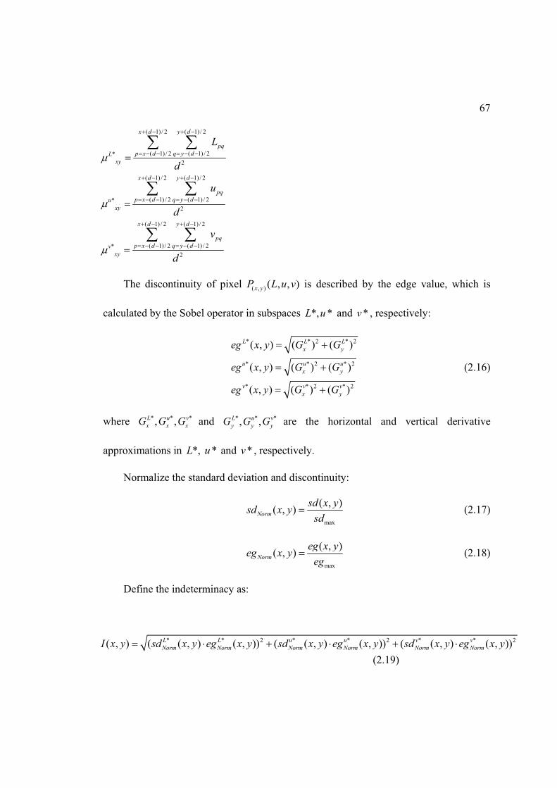
67

( 1) / 2 ( 1) / 2

( 1) / 2 ( 1) / 2*2

( 1) / 2 ( 1) / 2

( 1) / 2 ( 1) / 2*2

( 1) / 2 ( 1) / 2

( 1) / 2 ( 1) / 2*2

x d y d

pqp x d q y dL

xy

x d y d

pqp x d q y du

xy

x d y d

pqp x d q y dv

xy

L

d

u

d

v

d

The discontinuity of pixel ( , ) ( , , )x yP L u v is described by the edge value, which is

calculated by the Sobel operator in subspaces *, *L u and *v , respectively:

* * 2 * 2

* * 2 * 2

* * 2 * 2

( , ) ( ) ( )

( , ) ( ) ( )

( , ) ( ) ( )

L L Lx y

u u ux y

v v vx y

eg x y G G

eg x y G G

eg x y G G

(2.16)

where * * *, ,L u vx x xG G G and * * *, ,L u v

y y yG G G are the horizontal and vertical derivative

approximations in *, *L u and *v , respectively.

Normalize the standard deviation and discontinuity:

max

( , )( , )Normsd x ysd x y

sd (2.17)

max

( , )( , )Normeg x yeg x y

eg (2.18)

Define the indeterminacy as:

* * 2 * * 2 * * 2( , ) ( ( , ) ( , )) ( ( , ) ( , )) ( ( , ) ( , ))L L u u v vNorm Norm Norm Norm Norm NormI x y sd x y eg x y sd x y eg x y sd x y eg x y

(2.19)

68

Normalize I

max

( , )( , )NormI x yI x y

I (2.20)

Figure 4.4(e) is the indeterminacy image in domain I . The value of ( , )NormI x y has

a range of [0, 1]. The more uniform the region surrounding a pixel is, the smaller the

indeterminacy value of the pixel. The window size should be big enough to include

enough local information, but still smaller than the distance between two objects. We

chose d = 7 in our experiments.

4.2.6 Region Merging Based on ,E ET F , and NormI

The clusters segmented in ET are based on color information in an RGB space. The

edges in NormI include the spatial information in a CIE space. We get the final

segmentation result based on the following:

( ( ))i j norm i ji j

i j

true if R R and avg I R RR R

false otherwise (2.21)

where iR and jR are regions calculated in subsection 2.4. i jR R are intersection pixels

of regions iR and jR . ( ( ))norm i javg I R R is the average indeterminate value of the

intersection pixels.

Figure 4.4(f) is the final segmentation result of Lena based on NormI with 0.04 .

Figure 4.4(g) is the boundaries of (f). Adding indeterminacy reduces over-segmentation.

69

(a) (b) (c)

(d) (e) (f)

(g)

Figure 4.4. Steps of proposed algorithm: (a) 512x512 Lena color image. (b) Result after applying the S-function and enhancement. (c) Clusters result in T . (d) Boundaries based on (c). (e) Indeterminacy value image in I . (f) Final result of the proposed segmentation method ( 0.04 ). (g) Boundaries of (f).

70

4.3 Experimental Results

Domains T and F use the histograms, which include the global information.

Domain I includes the local information. By combining , T F and I , the proposed

algorithm can utilize both global and local information very well.

4.3.1 Parameter

Parameter is very important to performance. It controls the segmentation result.

The higher the value is, the fewer clusters there are in the segmentation result.

Figures 4.5(a), (b), and (c) show the results of = 0.01, 0.05, and 0.1. Figures 4.5(d), (e),

and (f) are the corresponding boundary images of (a), (b) and (c). The numbers of

clusters are 524, 393, and 290, respectively.

4.3.2 Comparison with Other Fuzzy Logic Algorithms

Neutrosophy is an extension to fuzzy logic. We now compare our approach with

several fuzzy logic color segmentation methods to show the advantage of neutrosophy.

Figure 4.6(a) is a 283x283 meadow image, and Figure 4.7(a) is a 256x256 house

image. Figure 4.6(b) and Figure 4.7(b) are the segmentation results after applying the

traditional fuzzy c-mean (FCM) algorithm, which is a widely used, unsupervised

segmentation method [13, 134-135]. Figure 4.6(c) and Figure 4.7(c) are the boundary

results of Figure 4.6(b) and Figure 4.7(b), respectively. There are 3757 regions in Figure

4.6(b) and 1673 regions in Figure 4.7(b). We can see that the traditional FCM produces

over-segmentation, and the boundaries are not clear. Figure 4.6(e) and Figure 4.7(e) are

the results of a modified FCM method (FCM_M) [23], which uses an adaptive method

71

to initialize cluster centers. It reduces over-segmentation (2913 regions in Fig. 5(e) and

1007 regions in Figure 4.7(e)) much better than does a traditional FCM. However, it still

includes over-segmentation on the right lower roof and eaves. Figure 4.6(f) and Figure

4.7(f) are the results of the proposed method (Neut). The over-segmentations are greatly

reduced (47 regions in Figure 4.6(f) and 69 regions in Figure 4.7(f)). Sheep boundaries

in Figure 4.6(f) and details of house edges in Figure 4.7(f) are kept very well. The

proposed method can outline main objects very well and has fewer regions than fuzzy c-

mean and modified fuzzy c-mean.

Figure 4.8(b) and Figure 4.9(b) are the segmentation results after using the fuzzy

homogeneity algorithm (FHM) in [136]. It utilizes a fuzzy homogeneity histogram and

scale-space filter to merge regions. Figure 4.8(d) and Figure 4.9(d) are the results after

using the proposed algorithm. In Figure 4.8(b), the shape of the airplane and mountains

are kept very well. The sailboat and ocean are clearly outlined in Figure 4.9(d). We can

see that the fuzzy homogeneity algorithm produces more over-segmented regions than

does our method (24410 regions in Figure 4.8(b) versus 251 regions in Figure 4.8(d);

and 18968 regions in Figure 4. 9(b) versus 101 regions in Figure 4. 9(d)). Figure 4.8(c)

and Figure 4.8(e) are the corresponding boundary images of 8(b) and 8(d), respectively.

The proposed method generates thinner, smoother, and clearer boundaries than does the

fuzzy homogeneity algorithm.

Table 4.3 lists the computation time of the proposed method on the different

images. The cluster selection is the most time-consuming step, which takes two-thirds of

72

the total time. All experiments were conducted by using Matlab 2008, Pentium D

3.00GHZ, and 3GB RAM.

Table 4.3. Running Time.

Image Name

Lena (512x512)

Meadow (283x283)

House (256x256)

Plane (469x512)

Sailboat (325x475)

CPU time (s)

24.2 7.3 6.1 20.1 13.5

4.4 Conclusions

In this chapter, a new neutrosophic method for color image segmentation is

proposed. It utilizes both RGB and CIE color spaces. By adding an indeterminacy

domain, the proposed algorithm can combine both global and local information as well

as information from two color spaces. Experimental results demonstrate that the

proposed method is very noise-tolerant, effective, and accurate, and it can generate thin

and clear boundaries in color segmentation results.

73

(a) (b) (c)

(d) (e) (f)

Figure 4.5. Segmentation results of different : (a) Segmentation result of 0.01. (b) Segmentation result of 0.05 . (c) Segmentation result of 0.1. (d) Boundaries of (a). (e) Boundaries of (b). (f) Boundaries of (c).

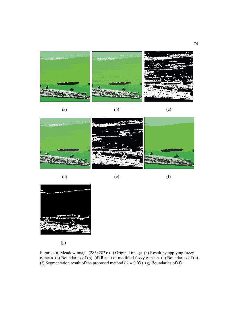
74

(a) (b) (c)

(d) (e) (f)

(g)

Figure 4.6. Meadow image (283x283): (a) Original image. (b) Result by applying fuzzy c-mean. (c) Boundaries of (b). (d) Result of modified fuzzy c-mean. (e) Boundaries of (e). (f) Segmentation result of the proposed method ( 0.03). (g) Boundaries of (f).

75

(a) (b) (c)

(d) (e) (f)

(g)

Figure 4.7. House image (256x256): (a) Original image. (c) Result by applying fuzzy c-mean. (c) Boundaries of (b). (d) Result of modified fuzzy c-mean. (e) Boundaries of (d). (f) Segmentation result of the proposed method ( 0.03). (g) Boundaries of (f).

76

(a) (b) (c)

(d) (e)

Figure 4.8. Plane image (469x512): (a) Original image. (b) Result by applying fuzzy homogeneity. (c) Boundaries of (b). (d) Segmentation result of the proposed method ( 0.04 ). (e) Boundaries of (d).

77

(a) (b) (c)

(d) (e)

Figure 4.9. Sailboat image (325x475): (a) Original image. (b) Result by applying fuzzy homogeneity. (d) Boundaries of (b). (d) Segmentation result of the proposed method ( 0.01). (e) Boundaries of (d).

78

CHAPTER 5

CONCLUSIONS

Neutrosophy studies the origin, nature, scope of neutralities, and their interactions

with different ideational spectra. It is an alternative to the existing logics and represents

mathematical uncertainty, vagueness, contradiction, and imprecision.

Neutrosophy is a new philosophy that is generating discussion among philosophers

and mathematicians. There is a need to find ways to implement neutrosophy in solving

problems. Researchers need exposure to how , ,T I F are defined and used in solving

real problems.

In this dissertation, I introduce neutrosophy to image segmentation and define

, ,T I F in image processing. T is the degree to be the object, I is the degree to be the

boundary, and F is the degree to be the background. Using neutrosophy in image

segmentation increases noise-tolerant ability, and it produces a superior blurry boundary

image as opposed to other methods. I apply the algorithm to breast ultrasound

segmentation, which is a real problem in medical image processing. Neutrosophy helps

to combine two controversial opinions about speckles: speckles are noise versus

speckles include pattern information. It is also a fully automatic segmentation algorithm

based on a whole BUS image not on a manually selected ROI. The experiment results

give us statistical improvements over other conventional image diagnostic methods. To

show neutrosophy in extended fuzzy logic, I use it in color image segmentation and

compare it with different fuzzy logic algorithms. The experiments demonstrate that

neutrosophy can reduce over-segmentation.

79

Neutrosophy is a new theory. It is an extension of fuzzy logic and can handle

uncertainty and indeterminacy better than other methods. Neutrosophy may find more

application in diverse fields, such as control theory, image processing, computer vision,

and artificial intelligence, where fuzzy logic is applied. The future works are described

as follows:

1. Neutrosophy is a new theory; the definition of indeterminacy can be defined in a

different way to include more uncertainty.

2. Neutrosophy can be applied to other image processing problems like feature

extraction and classification.

3. Apply neutrosophy to different research area like control theory, artificial

intelligence.

80

REFERENCES

1 Smarandache, F. A Unifying Field in Logics Neutrosophic Logic. Neutrosophy, Neutrosophic Set, Neutrosophic Probability. American Research Press, 2003.

2 Zhang, M., Zhang, L., and Cheng, H.D. A neutrosophic approach to image segmentation based on watershed method. Signal Processing 5, 90 (2010), 1510-1517.

3 L. A. Zadeh, Fuzzy sets. Information and Control 8, 3 (1965), 383-353.

4 Smarandache, F. Neutrosophy/Neutrosophic Probability, Set, and Logic.American Research, 1998.

5 S. Florentin, Collected Papers. Abaddaba, Oradea, III (2000).

6 Atanassov, K. Intuitionistic fuzzy sets. Fuzzy Sets and Systems 20, 1 (1986), 87-96.

7 Priest, G. Paraconsistent logic. Handbook of Philosophical Logic, vol 6, Kluwer, 2002.

8 Bruno, W. Dialetheism, logical consequence and hierarchy. Analysis 4, 64 (2004), 318-326.

9 Loeb, P. A. and Wolff, M. P. Nonstandard Analysis for the Working Mathematician. Kluwer, 2000.

10 Gonzalez, R.C. and Woods, R.E. Digital Image Processing. 3rd ed. Prentice Hall, 2007.

11 Deshmukh, K.S. and Shinde, G.N. An adaptive color image segmentation. Electronic Letters on Computer Vision and Image Analysis 5, 4 (2005), 12-23.

12 Shapiro, L.G. and Stockman, G.C. Computer Vision. Prentice-Hall, 2001.

13 Bezdek, J.C. Pattern Recognition with Fuzzy Objective Function Algorithms. New Plemm, 1981.

14 Haralick, R.M. and Shapiro, L.G. Survey: Image segmentation techniques. Computer Vision, Graphics and Image Processing 1, 29 (1985), 100-132.

81

15 V. I. Borisenko, A. A. Zlatopolskii, and I. B. Muchnik, Image segmentation (state-of-the-art survey). Automation and Remote Control 7, 48 (1987), 837-879.

16 Pal, N.R. and Pal, S.K. A review in image segmentation techniques. Pattern Recognition 9, 26 (1993), 1277-1294.

17 Y. J. Zhang, A survey on evaluation methods for image segmentation. PatternRecognition 8, 29 (1996), 1335-1346.

18 Zhang, H., Fritts, J.E., and Goldman, S.A. Image segmentation evaluation: A Survey of unsupervised methods. Computer Vision and Image Understanding 2,110 (2008), 260-280.

19 Spirkovska, L. A Summary of Image Segmentation Techniques. NASA Technical Memorandum, 104022, 1993.

20 Aghbari, Z.A. and Al-Haj, R. Hill-manipulation, An effective algorithm for color image segmentation. Image and Vision Computing 24, 8 (2006), 894-903.

21 Bleau, A. and Leon, L.J. Watershed-based segmentation and region merging. Computer Vision and Image Understanding 3, 77 (2000), 317-370.

22 Jiang, Y. and Zhou, Z.-H. SOM ensemble-based image segmentation. Neural Processing Letters 3, 20 (2004), 171-178.

23 Yu, Z., Zou, T., and Yu, S. A modified fuzzy C-Means algorithm with adaptive spatial information for color image segmentation. Computational Intelligence for Image Processing, 2009, 48-52.

24 Glasbey, C.A. An analysis of histogram-based thresholding algorithms. Graphical Models and Image Processing 6, 55 (1993), 532-537.

25 Kapur, J.N., ahoo, P.K., and Wong, A.K.C. A new method for graylevel picture thresholding using the entropy of the histogram. Computer Vision Graphics, and Image Processing 3, 29 (1985), 273-285.

26 Alvarez, L., Lions, P.L., and Morel, J.-M. Image selective smoothing and edge detection by nonlinear diffusion, II. SIAM Journal on Numerical Analysis 29, 3 (1992), 845-866.

27 Pollak, I., Willsky, A.S., and Krim, H. Image segmentation and edge enhancement with stabilized inverse diffusion equations. IEEE Trans. on Image Processing 2, 9 (2000), 256-266.

82

28 Tabb, M. and Ahuja, N. Multiscale image segmentation by integrated edge and region detection. IEEE Trans. on Image Processing 5, 6 (1997), 642-655.

29 Freixenet, J., Muñoz, X., Raba, D., Martí, J., and Cufí, X. Yet another survey on image segmentation: Region and boundary information integration. Lecture Notes in Computer Science 2352 (2002), 408 - 422.

30 Campbell, J.G., Fraley, C., Murtagh, F., and Raftery, A.E. Linear flaw detection in woven textiles using model-based clusterin. Pattern Recognition Letters 14, 18 (1997), 1539-1548.

31 Murtagha, F., Rafteryb, A.E., Starck, J.-L. Bayesian inference for multiband image segmentation via model-based cluster trees. Image and Vision Computing 6,23 (2005), 587-596.

32 Najman, L. and Schmitt, M. Watershed of a continuous function. Signal Processing (Special Issue on Mathematical Morphology) 1 38 (1994), 99-112.

33 Cousty, J., Bertrand, G., Najman, L., and Couprie, M. Watershed cuts: Minimum spanning forests and the drop of water principle. IEEE Trans. on Pattern Analysis and Machine Intelligence 8, 31 (2009), 1362–1374.

34 Tann, H., Gelfand, S., and Delpf, E. A comparative cost function approach to Edge Detection. IEEE Trans. On Systems, Man, And Cybernetics 6, 19 (1989).

35 Najman, L. and Schmitt, M.Watershed of a continuous function. SignalProcessing (Special Issue on Mathematical Morphology.) 1, 38 (1994), 99-112.

36 Najman, L. and Schmitt, M. Geodesic saliency of watershed contours and hierarchical segmentation. IEEE Trans. on Pattern Analysis and Machine Intelligence 12, 18 (1996), 1163-1173.

37 Najman, L., Couprie, M., and Bertrand, G.Watersheds, mosaics, and the emergence paradigm. Discrete Applied Mathematics 2-3, 147 (2005), 301-324.

38 Li, P. and Xiao, X. Multispectral image segmentation by a multichannel watershed-based approach. International Journal of Remote Sensing 19, 28 (2007), 4429-4452.

39 Wang, D. A multiscale gradient algorithm for image segmentation using watersheds. Pattern Recognition 12, 30 (1997), 2043-2052.

83

40 Cheng, H.D. and Chen, J.R. Automatically determine the membership function based on the maximum entropy principle. Information Sciences 3-4, 96 (1997), 163-182.

41 Cheng, H.D., Wang, J.L., and Shi, X.J. Microcalcification detection using fuzzy logic and scale space approach. Pattern Recognition 2, 37 (2004), 363-375.

42 Cheng, H.D. and Li, J.G. Fuzzy homogeneity and scale space approach to color image aegmentation. Pattern Recognition 35 (2002), 373-393.

43 Pal, S.K. and Majumder, D.K.D. Fuzzy Mathematical Approach to Pattern Recognition. Wiley, 1986.

44 H. D. Cheng, H. Xu, A Novel fuzzy logic approach to contrast enhancement. Pattern Recognition, 5, 33 (2000), 809-919.

45 Ross, T. Fuzzy Logic with Engineering Applications, 3rd ed. Wiley, 2010.

46 Vincent, L. and Soille, P. Watersheds in digital spaces: an efficient algorithm based on immersion simulations. IEEE Trans. on Pattern Analysis and Machine Intelligence 6, 13 (1991), 583-598.

47 Beucher, S. and Meyer, F. The morphological approach to segmentation: the watershed transformation. Mathematical Morphology in Image Processing (1993), 433-481.

48 Meer, P. and Georgescu, B. Edge detection with embedded confidence. IEEETrans. on Pattern Analysis and Machine Intellelligence 12, 23 (2001), 1351-1356.

49 Robust Image Understanding Lab. 2002. http://coewww.rutgers.edu/riul/research/ code/EDISON/doc/overview.html. May 5, 2009.

50 Comaniciu, D. and Meer, P. Mean shift: A robust approach toward feature space analysis. IEEE Trans. on Pattern Analysis and Machine Intelligence 5, 24 (2002), 603-619.

51 Lin, Y.C., Tsai, Y.P., Hung, Y.P., and Shih, Z.C. Comparison between immersion-based and toboggan-based watershed image segmentation. IEEE Trans. on Image Processing 3, 15 (2006), 632-640.

52 Garcia, M., Jemal, A., Ward, E., Center, M., Hao, Y., Siegel, R., and Thun, M. Global Cancer Facts & Figures 2007. American Cancer Society, 2007.

84

53 American Cancer Society. Cancer Facts & Figures 2008. American Cancer Society, 2008.

54 Jemal, A. Murray, T., Ward, E., Samuels, A., Tiwari, R.C., A. Ghafoor, A., Feuer, E.J., and Thun, M.J. Cancer statistics 2008. CA: Cancer J. for Clinicians 58, 2 (2008), 71-96.

55 Jemal, A., Siegel, R., Xu, J., and Ward, E. Cancer statistics 2010. CA: Cancer J. for Clinicians 60, 5 (2010), 1-24.

56 American Cancer Society. Cancer Facts & Figures 2009. American Cancer Society, 2009.

57 Cheng, H.D., Cai, X.P., Chen, J.W., Hu, L.M., and Lou, X.L. Computer-aided detection and classification of microcalcifications in mammograms: A survey. Pattern Recognition 12, 36 (2003), 2967-2991.

58 Cheng, H.D., Shi, X.J., Min, R., Hu, L.M., Cai, X.P., Du, H.N. Approaches for automated detection and classification of masses in mammograms. Pattern Recognition,4, 39 (2006), 646-668.

59 Joseph, Y.L. and Carey, E.F. Application of artificial neural networks for diagnosis of breast cancer. In Proceedings of the Congress of Evolutionary Computation, 1999, 1755-1759.

60 Kopans, D.B. The positive predictive value of mammography. American Journal of Roentgenology 158, 3 (1992), 521-526.

61 Knutzen, A.M. and Gisvold, J.J. Likelihood of malignant disease for various categories of mammographically detected, nonpalpable breast lesions. MayoClinic Proceedings, 68, 5 (1993), 454-460.

62 Breastcancer.org. Ultrasound. 2009. http://www.breastcancer.org/symptoms/ testing/types/ultrasound.jsp. Jan. 2009.

63 Breastcancer.org. Mammography: Benefits, Risks, What You Need to Know. 2008. http://www.breastcancer.org/symptoms/testing/types/mammograms/ benefits_risks.jsp. Jan. 2009.

64 Jackson, V.P., Hendrick, R.E., Feig, S.A., and Kopans, D. Imaging of the radiographically dense breast. Radiology 188, 2 (1993), 297-301.

85

65 Sivaramakrishna, R., Powell, K.A., Lieber, M.L., Chilcote, W. and Shekhar, R.Texture analysis of lesions in breast ultrasound images. Computerized Medical Imaging and Graphics 26, 5 (2002), 303-307.

66 Drukker, K., Giger, M.L., Horsch, K., Kupinski, M.A., Vyborny, C.J., and Mendelson, E.B. Computerized lesion detection on breast ultrasound. Medical Physics 7, 29 (2002), 1438-1446.

67 Taylor, K., Merritt, C., Piccoli, C., R. Schmidt, R., G. Rouse, G., B. Fornage, B., E. Rubin, E., D. Georgian-Smith, D., Winsberg, F., Goldberg, B., and Mendelson, E. Ultrasound as a complement to mammography and breast examination to characterize breast masses. Ultrasound in Medicine and Biology 28, 1 (2002), 19-26.

68 Bassett, L.W., Ysrael, M., Gold, R.H., and Ysrael, C. Usefulness of mammography and sonography in women less than 35 years of age. Radiology180, 3 (1991), 831.

69 John, C., Blohmer, J.U., and Hamper, U.M. Breast Ultrasound: A Systematic Approach to Technique and Image Interpretation. Thieme, 1999.

70 Laine, H., Rainio, J., Arko, H., and Tukeva, T. Comparison of breast structure and findings by X-ray mammography, ultrasound, cytology and histology: A retrospective study. European Journal of Ultrasound 2, 2 (1995), 107-115.

71 Jackson, V.P. The role of ultrasound in breast imaging. Radiology 177, 2 (1990), 305-311.

72 Wikipedia. Medical imaging. http://en.wikipedia.org/wiki/Medical_image_ processing#Ultrasound. Jan. 2009.

73 Hu, L.M., Cheng, H.D., Zhang, M. A high performance edge detector based on fuzzy inference rules. Information Sciences 21, 177 (2007), 4768-4784.

74 Guo, Y.H., Cheng, H.D.,Tian, J, and Zhang, Y.T. A novel approach to speckle reduction in ultrasound imaging. Ultrasound in Medicine and Biology 4, 35 (2009), 628-640.

75 Chang, R.F., Wu, W.J., Moon, W.K., and Chen, D.R. Improvement in breast tumor discrimination by support vector machines and speckle-emphasis texture analysis. Ultrasound in Medicine and Biology 5, 29 (2003), 679-686.

86

76 Alemán-Flores, M., Álvarez, L., and Caselles, V. Texture-oriented anisotropic filtering and geodesic active contours in breast tumor ultrasound segmentation. Journal of Mathematical Imaging and Vision 1, 28 (2007), 81-97.

77 Yeh, C.-K., Chen, Y.-S., Fan, W.-C., and Liao, Y.-Y. A disk expansion segmentation method for ultrasonic breast lesions. Pattern Recognition 5, 42 (2009), 596-606.

78 Noble, J.A. and Boukerroui, D. Ultrasound image segmentation: A survey. IEEE Trans. on Medical Imaging 8, 25 (2006), 987-1010.

79 Duta, N. and Sonka, M. Segmentation and interpretation of MR brain images: An improved active shape model. IEEE Trans. Medical Imaging 6, 17 (1998), 1049-1062.

80 Mignotte, M., Meunier, J., and Tardif, J.C. Endocardial boundary estimation and tracking in echocardiographic images ssing deformable template and Markov random fields. Pattern Analysis and Applications 4, 4 (2001), 256-271.

81 Hao, X., Bruce, C.J., Pislaru, C., and Greenleaf, J.F. Segmenting high-frequency intracardiac ultrasound images for myocardium into infarcted, ischemic and normal regions. IEEE. Trans. on Medical Imaging 122, 20 (2001), 1373–1383.

82 Madabhushi, A. and Metaxas, D.N. Combining low-, high-level and empirical domain knowledge for automated segmentation of ultrasonic breast lesions. IEEE Trans. on Medical Imaging 2, 22 (2003), 155-169.

83 Montagnat, J., Sermesant, M., Delingette, H., Malandain, G., and Ayache, N. Anisotropic filtering for model-based segmentation of 4-D cylindrical echocardiographic images. Pattern Recognition Letters 4-5, 24 (2003), 815-828.

84 Ashton, E.A. and Parker, K.J. Multiple resolution Bayesian segmentation of ultrasound images. Ultrasound Image 17, 4 (1995), 291-304.

85 Boukerroui, D., Baskurt, A., Noble, J.A., and Basset, O. Segmentation of ultrasound images multiresolution 2D and 3D algorithm based on global and local statistics. Pattern Recognition Letters 12, 24 (2003), 1373-1383.

86 Mousa, R., Munib, Q., and Moussa, A. Breast cancer diagnosis system based on wavelet analysis and fuzzy-neural. Expert Systems With Applications 4, 28 (2005), 713-723.

87 Kirberger, R.M. BVSc, mmedVet, Imaging artifacts in diagnostic ultrasound-A Review. Veterinary Radiology & Ultrasound 4, 36 (2005), 297 - 306.

87

88 Paragios, N. and Deriche, R. Geodesic active contours and level sets for the detection and tracking of moving objects. IEEE Trans. on Pattern Analysis Machine Intelligence 3, 22 (2000), 266-280.

89 Chalana, V. and Kim, Y. A methodology for evaluation of boundary detection algorithms on medical images. IEEE Trans. on Medical Imaging 5, 16 (1997), 642-652.

90 Kim, U.H., Seo, B.K., Lee, J., Kim, S.J., Cho, K.R., and Lee, K.Y. Correlation of ultrasound findings with histology, tumor grade, and biological markers in breast cancer. Acta Oncologica 8, 47 (2008), 1531-1538.

91 Chan, T.F. and Vese, L.A. Active contours without edges. IEEE Trans. on Image Processing 2, 10 (2001), 266-277.

92 Chan, T.F. and Vese, L.A. A multiphase level set framework for image segmentation using the Mumford and Shah model. International J. of Computer Vision 50, 3 (2002), 271-293.

93 Chen, D.R., Chang, R.F., Wu, W.J., Moon, W.K., and Wu, W.L. 3-D Breast ultrasound segmentation using active contour model. Ultrasound Medicine and Biology 7, 29 (2003), 1017-1026.

94 Liu, B., Cheng, H.D., Huang, J.H., Tian, J.W., Tang, X.L., and Liu, J.F. Fully automatic and segmentation-robust classification of breast tumors based on local texture analysis of ultrasound images. Pattern Recognition 1, 43 (2010), 280-298.

95 Cheng, H.D., Shan, J., Ju, W., Guo, Y.H., and Zhang, L. Automated breast cancer detection and classification using ultrasound images: A survey. Pattern Recognition 1, 43 (2010), 299-317.

96 Warfield, S.K., Zou, K.H., Kaus, M.R., and Wells, W.M. Simultaneous validation of image segmentation and assessment of expert quality. In Proceedings IEEE International Symposium on Biomedical Imaging, 2002, 94–97.

97 Cheng, H.D., Jiang, X.H., Sun, Y., and Wang, J.L. Color image segmentation: Advances and prospects. Pattern Recognition 12, 34 (2001), 2259-2281.

98 Mao, X., Zhang, Y., Hu, Y., and Sun, B. Color image segmentation method based on region growing and ant colony clustering. IEEE Computer Society 1 (2009), 173-177.

88

99 Special issue on digital libraries: representation and retrieval. IEEE Trans. on Pattern Analysis and Machine Intelligence, 8, PAMI-18 (1996).

100 Special issue on segmentation, description, and retrieval of video content. IEEE Trans. on Circuits and Systems for Video Technology, 5, CASVT-8 (1998).

101 Pietikainen, M. Accurate color discrimination with classification based on feature distributions. In International Conference on Pattern Recognition, 1996, 833-838.

102 Littmann, E. and Ritter, H. Adaptive color segmentation --a comparison of neural and statistical methods. IEEE Trans. on Neural Networks 8, 1 (1997), 175-185.

103 Huntsberger, T.L., Jacobs, C.L., and Cannon, R.L. Iterative fuzzy image segmentation. Pattern Recognition 18, 2 (1985), 131-138.

104 Kim, W.S. and Park, R.H. Color image palette construction based on the HSI color system for minimizing the reconstruction error. In IEEE International Conference on Image Processing, 1996, 1041-1044.

105 Hoy, D.E.P. On the use of color imaging in experimental applications. Experimental Techniques 21, 4 (1997), 17-19.

106 Robinson, G.S. Color edge detection. Optical Engeering 16, 5 (1997), 479-484.

107 Tseng, D.C. and Chang, C.H. Color segmentation using perceptual attributes. In IEEE International Conference on Pattern Recognition, 1992, 228-231.

108 Pal, S.K. A review on image segmentation techniques. Pattern Recognition 29,(1993), 1277-1294.

109 Yang, C.K. and Tsai, W.H. Reduction of color space dimensionality by moment-preserving thresholding and its application for edge detection in color images,. Pattern Recognition Letters 5, 17 (1996), 481-490.

110 Tremeau, A. and Borel, N. A region growing and merging algorithm to color segmentation. Pattern Recognition 7, 30 (1997), 1191-1203.

111 Kato, Z. and Pong, T. A Markov random field image segmentation model for color textured images. Image and Vision Computing 10, 24 (2006), 1103-1114.

112 Littmann, E. and Ritter, H. Adaptive color segmentation - a comparison of neural and statistical methods,. IEEE Trans. on Neural Networks 8, 1 (1997), 175-185.

89

113 Fu, K.S. and Mui, J.K. A survey on image segmentation. Pattern Recognition 13,1 (1981), 3-16.

114 Macaire, L., Ultre, V., and Postaire, J.-G. Determination of compatibility coe$cients for color edge detection by relaxation. In International Conference on Image Processing, (1996), 1045-1048.

115 Nevatia, K. A color edge detector and its use in scene segmentation. IEEE Trans. on Systems, Man Cybernetics 11, 7 (1977), 820-826.

116 Trahanias, P.E. and Venetsanopoulos, A.N. Color edge detection using vector order statistics. IEEE Trans. Image Processing 2, 2 (1993), 259-265.

117 Trahanias, P.E. and Venetsanopoulos, A.N. Vector order statistics operators as color edge detectors. IEEE Trans. Systems Man Cybernet.-Part B: Cybernetics 26,1 (1996), 135-143.

118 Ohta, Y., Kanade, T., and Sakai, T. Color information for region segmentation. Computer Graphics Image Processing 3, 13 (1980), 222-241.

119 Ohlander, R., Price, K., and Reddy, D.R. Picture segmentation using a recursive region splitting method. Computer Graphics Image Processing 3, 8 (1978), 313-333.

120 Tominaga, S. Color image segmentation using three perceptual attributes. In Proceedings of the IEEEConference on Computer Vision and Pattern Recognition,1986, 628-630.

121 Lescure, P., Meas-Yedid, V., Dupoisot, H., and Stamon, G. Color segmentation on biological microscope images. In Proceeding of SPIE, Application of Artificial Neural Networks in Image Processing IV, (1999), 182-193.

122 Rae, R. and Ritter, H.J. Recognition of human head orientation based on artificial neural networks. IEEE Trans. on Neural Network, 9, 2 (1998), 257-265.

123 C.-L. Huang, Pattern image segmentation using modified Hopfield model. PatternRecognition Letters, 3, 15 (1999), 345-353.

124 Campadelli, P., Medici, D., and Schettini, R. Color image segmentation using Hopfield networks. Image Vision Computing 3, 15 (1997), 161-166.

125 Vesanto, J. and Alhoniemi, E. Clustering of the self-organizing map. IEEE Trans. on Neural Networks 11, 3 (2000), 586-600.

90

126 Ji, S. and Park, H.W. Image segmentation of color image based on region coherency. In International Conference on Image Processing, 1998, 80-83.

127 Lo, Y.S. and Pei, S.C. Color image segmentation using local histogram and self-organization of Kohonen feature map. In International Conference on Image Processing, 1999, 232-239.

128 Keller, J.M.,Gray, M.R., and Givens, J.A. A fuzzy K-nearest neighbor algorithm. IEEE Trans. on Systems, Man Cybernetics 4, SMC-15 (1985), 580-585.

129 Keller, J.M. and Carpenter, C.L. Image segmentation in the presence of uncertainty. International Journal of Intelligent Systems 2, 5 (1990), 193-208.

130 Bezdek, J.C. and Castelaz, P.F. Prototype classification and feature selection with fuzzy sets. Pattern Recognition Letters 14, (1993), 483-488.

131 Nock, R. and Nielsen, F. Semi-supervised statistical region refinement for color image segmentation. Pattern Recognition 6, 38 (2005), 835-846.

132 Robinson, G. Color edge detection. Optical Engineering 16, 5 (1977), 479-484.

133 Fairchild, M.D. Color Appearance Models. Addison-Wesley, 1998.

134 Ruspini, E. Numerical methods for fuzzy clustering. Information Sciences 3, 2 (1970), 319-350.

135 Dunn, J.C. A fuzzy relative of the ISODATA process and its use in detecting compact, well separated clusters. Cybernetics 3, 3 (1974), 95-104.

136 Cheng, H.D. and Li, J. Fuzzy homogeneity and scale-space approach to color image segmentation. Pattern Recognition 7, 36 (2003), 1545-1562.

91

CURRICULUM VITAE

Ming Zhang (November, 2010)

EDUCATION

Ph.D., Computer Science 12/ 2010

Utah State University, Logan, UT GPA 3.9

Advisor: Prof. Heng-Da Cheng

B.Eng., Computer Science 07/2001

Shandong University, Jinan, Shandong, China GPA 3.8

RESEARCH INTERESTS

Computer Vision Pattern Recognition

Image Processing Medical Image Processing

Fuzzy Logic Neutrosophy

RESEARCH AND WORK EXPERIENCE

Teaching Assistant 08/2004 – present

School of Computer Science, Utah State University Logan, UT

Graded computer algorithms, parallel computing, digital image processing,

software engineering, and pattern recognition.

Tutored all levels of computer science undergraduate students.

92

System Administrator 06/2006 – 12/2008

Department of Economics, Utah State University Logan, UT

Managed department servers (DNS, email, ftp, backup) and department

computers.

Protected computers from being attacked.

Group member of CVPRIP lab 04/2005 – present

School of Computer Science, Utah State University Logan, UT

Research on breast cancer segmentation and classification in CVPRIP (Computer

Vision, Pattern Recognition, Image Processing) Lab. The research is for breast

cancer mass detection based on ultrasound images.

Introduced neutrosophy to ultrasound image processing.

Designed and implemented pavement crack detection system, a real-time system

created to detect cracks in asphalt and concrete roads.

Designed and implemented vehicle detection and classification system. It uses a

model-based method to develop an automatic video-based intelligent feature

extraction system. The images were captured by the highway traffic control office

of Utah Department of Transportation (UDOT).

Software Programmer 07/2001 – 09/2003

Xu Ji Company Jinan, China

Created power plant information collecting system. The system uses palm to

collect the diagonal information within the power plant per hour and transfer them

to the corresponding departments.

93

Pre-designed a call center system which serves as customer service for the Power

Bureau.

Internship 02/2001 – 07/2001

Xian Dai Company Jinan, China

Implemented work sheet system for power plants

Research Assistant 09/1998 – 07/2000

Shandong University Jinan, China

Served as research assistant in EBM (Electron Beam) Lab

Participated in developing diagnostic system for diesel engine status

Participated in developing the Automatic Check system for vehicle headlight

Provided computer maintenance

Conference Reviewer

Reviewed papers of 8th Joint Conference on Information Science 03/2005

Reviewed papers of 11th Joint Conference on Information Science 03/2008

AWARDS AND HONORS

Teaching Assistant, Computer Science, 2004 – present

Dissertation Fellowship, 2008 – 2009

Graduate Studies Honor Roll, 2003 – 2004

Vice Presidential Fellowship, 2003 – 2004

Scholarship Recipient, 1997 – 1998, 1998 – 1999, 1999 – 2000, 2000 – 2001

Ping Pong Champion, Utah State University, 2003 – 2007

94

SELECTED PUBLICATIONS

Journals

Zhang, M., Cheng, H. D., Color Segmentation Based on Neutrosophic Method,

Pattern Recognition, (under review).

Zhang, M., Zhang, L., Cheng, H. D., Segmentation of Breast Ultrasound Images

Based on Neutrosophic Method, Optical Engineering, (in press).

Zhang, M., Zhang, L., Cheng, H. D., A Neutrosophic Approach to Image

Segmentation Based on Watershed Approach, Signal Processing, 90(5), 1510-1517,

2010

Cheng, H. D., Min, R., Zhang, M., Automatic Wavelet base selection and its

application to contrast enhancement, Signal Processing, 90(4), 1279-1289, 2010

Hu, L.M., Cheng, H. D., Zhang, M., A High Performance Edge Detector Based on

Fuzzy Inference Rules, Information Science, 177(21): 4768-4784, 2007

Cheng, H. D., Xue, M., Shi, X. J., Zhang, M., Novel Contrast Enhancement

Approach Based on Fuzzy Homogeneity, Optical Engineering, 46(4), 047002, 2006.

Zhang, M., Study on Conductivity Measurement of Metal with High Temperature,

Measurement Technique, No. 6, 6-8, June 2002 (in Chinese).

Conferences

Zhang, L., Zhang, M., An Extended Fuzzy Logic Method for Watershed, Proc. 11th

Join Conference of Information Science, 2008.

Zhang, M., Zhang, L., Fuzzy Watershed Method for Image Segmentation, Proc. 10th

95

Join Conference of Information Science, 2007.

Zhang, L., Sun, Y., Zhang, M., Lightweight RTPS Middleware for Distributed

SCADA System, Proc. 10th Join Conference of Information Science, 2007.