Notes on General Equilibrium - personalpages.manchester.ac.uk · Reference: Jehle and Reny, Advanced Microeconomic Theory, 3rd ed., Pearson 2011: Ch. 5. Behind the superﬁcial chaos

Notes on General Equilibrium

Alejandro Saporiti

Alejandro Saporiti (Copyright) General Equilibrium 1 / 42

General equilibrium

Reference:Jehle and Reny,Advanced Microeconomic Theory, 3rd ed.,Pearson 2011: Ch. 5.

Behind the superficial chaos of countless market transactions by selfishindividuals, Adam Smith (1776) saw a harmonizing force (theinvisible hand)operating in a competitive economy.

Smith believed that force guides individuals tocoordinatetheir choices, i.e.their consumption and productions plans, in such a way that all markets in theeconomy are brought into balance simultaneously.

He also believed that the resultingequilibriumpossessessocially desirableproperties, in the sense that it maximizes social welfare through no consciouscollective intention of its members.

Does this vision of the competitive markets possess any substance?


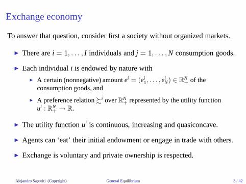
Exchange economy

To answer that question, consider first a society without organized markets.

◮ There arei = 1, . . . , I individuals andj = 1, . . . , N consumption goods.

◮ Each individuali is endowed by nature with

◮ A certain (nonnegative) amountei = (ei1, . . . , ei

N) ∈ RN+ of the

consumption goods, and

◮ A preference relation%i overRN+ represented by the utility function

ui : RN+ → R.

◮ The utility functionui is continuous, increasing and quasiconcave.

◮ Agents can ‘eat’ their initial endowment or engage in trade with others.

◮ Exchange is voluntary and private ownership is respected.


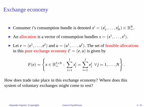
Exchange economy

◮ Consumeri’s consumption bundle is denotedxi = (xi1, . . . , xi

N) ∈ RN+.

◮ An allocationis a vector of consumption bundlesx = (x1, . . . , xI ).

◮ Let e = (e1, . . . , eI ) andu = (u1, . . . , uI ). The set offeasible allocationsin this pure exchange economyE = (e, u) is given by

F(e) =

{

x ∈ RI×N+ :

I∑

i=1

xij =

I∑

i=1

eij ∀ j = 1, . . . , N

}

.

How does trade take place in this exchange economy? Where does thissystem of voluntary exchanges might come to rest?


Bilateral exchange

To simplify the analysis, let’s focus on a2× 2 economy, i.e., an economywith two consumers,A andB, and two goods, 1 and 2.

The main advantage of the 2× 2 economy is that it can be graphicallydescribed through the so calledEdgeworth box.

The Edgeworth box has heighteA2 + eB

2 and widtheA1 + eB

1 , and every pointxrepresents a feasible allocation, where for allj = 1, 2,

xAj + xB

j = eAj + eB

j .

The box offers a complete picture of every feasible distribution of the existingcommodities between the consumers.


The Edgeworth box

0

0

A

0

0

B

xA1

xA2

xB1

xB2

eA1

eB2

eB1

eA2

e

A andB’s initialendowments are givenby (eA

1 , eA2) and(eB

1 , eB2).

All bundles inside theindifference lenticularare preferred toebybothA andB.

To achieve these gains,consumers mustexchange part of theirinitial endowments.


The Edgeworth box

0

0

A

0

0

B

xA1

xA2

xB1

xB2

eA1

eB2

eB1

eA2

yA1

yB2

yB1

yA2

y

e

For instance,y ispreferred bybothAandB to theirinitial endowment.

But y doesn’texhaust thepossibilities forbeneficial tradebetweenA andB.


The Edgeworth box

0

0

A

0

0

B

xA1

xA2

xB1

xB2

eA1

eB2

eB1

eA2

zA1

zB2

zB1

zA2

z

e

Only at a point likezthere are no moremutually beneficialtrades betweenA andB.

The ‘no worse than’(upper counter) setstouch only atz.


Pareto efficiency

We would expect rational agents will trade until all possibilities for mutuallybeneficial trade are exhausted. Such allocations are said tobePareto efficient.

Definition 1 (Pareto efficiency in consumption)A feasible allocationz∈ F(e) is said to bePareto efficient (PE)if there is noother feasible allocationz∈ F(e) such thatui (zi) ≥ ui(zi) for all i = 1, . . . , I ,with strict inequality for somei.

Geometrically in the Edgeworth box, PE allocations are points x = (xA, xB) atwhich consumers’ indifference curves are tangent; i.e., points at which themarginal rates of substitution are all equal:

MRSA1,2(x

A1 , xA

2) = MRSB1,2(x

B1 , xB

2). (1)


Pareto efficiency

Figure 1:Pareto efficiency in consumption.

Definition 2 (Contract curve)The setCC of all feasible and Pareto efficient allocations is called the Paretosetor contract curve.


Contract curve and the coreCore: set of possible

equilibrium which

OBy

equilibrium which

improve utility

relative to

endowment, e2

3e

1e 2e

OAx

Contract Curve:

Locus of points of

tangency between MRStangency between MRS

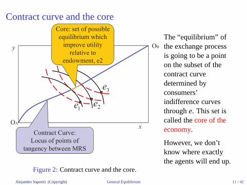
Figure 2:Contract curve and the core.

The “equilibrium” ofthe exchange processis going to be a pointon the subset of thecontract curvedetermined byconsumers’indifference curvesthroughe. This set iscalled thecore of theeconomy.

However, we don’tknow where exactlythe agents will end up.


Generalizing the core

Definition 3 (Blocking coalitions)A set of agentsSblocksx ∈ F(e) if there exists an allocationy such that (i)∑

i∈Syi =∑

i∈Sei , and (ii)ui(yi) ≥ ui(ei) for all i ∈ S, with strict inequalityfor somei.

Definition 4 (The core)The core of an exchange economyE = (e, u), denoteC(E), is the set of allunblocked feasible allocations.

Apart from the the fact that the core might be “pretty big” (see Fig. 2) andtherefore lack any prediction power, the amount of information needed toarrange mutually beneficial trade and converge toC(E) might also be huge!

The next step is to examine howmarket economiesdeal with these problems.


Competitive markets

Let’s now add to our primitive economyE = (e, u) of pure exchange a fewother assumptions:

◮ Markets existfor all goods.

◮ Agents canfreely participatein markets without cost.

◮ “Standard” consumer theory assumptions:

◮ Preferences (strictly) monotone & represented by utility function;◮ Some “convexity” if needed;◮ All agents are price-takers;◮ Finite number of perfectly divisible goods;◮ Linear prices;◮ Perfect information about goods and prices.

◮ All agents face thesame prices.


Walrasian equilibrium

Given pricesp ≫ 0, denote byyi(p) =∑

j pj eij consumeri’s initial income,

and byBi(p) = {xi ∈ RL+ : p · xi ≤ yi(p)} the budget set fori.

Definition 5 (Walrasian equilibrium)A price vectorp = (p1, . . . , pN) and an allocationx = (x1, . . . , xI ) are said tobe aWalrasian or competitive equilibrium (WE)iff

(i) For all i = 1, . . . , I , xi ∈ arg maxx∈Bi(p) ui(x); i.e.,xi is consumeri’sWalrasian demand at pricesp and incomeyi(p); and

(ii) Markets clear atp; i.e, for all j = 1, . . . , N, the excess demand function

zj(p) ≡I

∑

i=1

xij −

I∑

i=1

eij = 0.


Walrasian equilibriumIn words, a WE is a set of prices such that

(i) Each agent chooses hismost-preferredaffordable bundle; and

(ii) Consumers’ choices arecompatibleamong each other, in the sense thattotal demand equals total supply in every market.

Actually, this definition of a WE is stronger than necessary:It turns out that ifthe aggregate excess demand forN − 1 goods is zero, then the excess demandfor the remaining good must be zero too.

This follows from a property of the excess demand function called Walras’law: the value of the aggregate excess demand is zero forall possible prices(see Exercise 3.1):

N∑

j=1

pj zj(p1, . . . , pN) = 0.


Walrasian equilibrium

Theoffer curvetracesout Walrasian demandas prices change.

Walrasian equilibriaare at the intersectionof the offer curves.

The intersection andthereby the Walrasianequilibrium need notbe unique.


Equilibrium existenceFor arbitrary prices(p1, p2) there is no guarantee that supply will equaldemand, i.e., there is no guarantee that (ii) is satisfied.

Figure 3:No equilibrium.


Equilibrium existence

How do we know that there exists a set of prices such that (i) and (ii) aresimultaneously satisfied?

This is known as the question of the existence of a competitive equilibrium.

Early economists thought that equilibrium prices would always exist becausethe system hasN − 1 independent (excess demand) equations (by Walras’law) andN − 1 independent prices.

◮ There are in factN prices, but we are free to choose one of the prices andset it equal to a constant, namely, equal to 1 (recall Walrasian demandsare homogeneous of degree zero in prices).

◮ This price plays the role ofnumeraire, and all other prices are measuredrelative to it.


Equilibrium existenceHowever, counting the number of equations and unknowns is not sufficient toprove that a WE exists.

Wald (1936) was the first to points out Walras’ error by offering a simplecounterexample:x2 + y2 = 0 andx2 − y2 = 1.

The key issue is to ensure thatthe aggregate excess demandfunction iscontinuous(less thanthat is actually necessary).

That means that a small changein the prices shouldn’t result ina big jump in the quantitydemanded.

p1

z1(p1)

Figure 4:Two goods.Alejandro Saporiti (Copyright) General Equilibrium 19 / 42

Excess demand

Under what conditions will the aggregate excess demand functions becontinuous?

Definition 6 (Excess demand)Theexcess demand of agenti is zi(p) = xi(p, yi(p)) − ei , wherexi(p, yi(p)) isi’s Walrasian demand at pricesp and incomeyi(p) = p · ei . Theaggregateexcess demandis z(p) =

∑Ii=1 zi(p).

Note that a WE is a price vectorp∗ ∈ RN+ such thatz(p∗) = 0.

Some of the properties of the aggregate excess demand are thefollowing.


Properties of the excess demand

Supposeui is continuous, increasing, and concave, andei ≫ 0 for all i.

◮ z(·) is continuous.

◮ Continuity ofui implies continuity of Walrasian demandxi(p, yi(p)).

◮ z(·) homogenous of degree zero(only relative prices matter).

◮ xi(p, yi(p)) homogeneous of degree zero inp.◮ zi(p) = xi(p, yi(p)) − ei homogeneous of degree zero inp.◮

∑

i zi(p) homogeneous of degree zero inp.◮ Therefore, we cannormalize one price⇒ N − 1 unknowns.

◮ z(·) verifies Walras’ law; i.e.,p · z(p) = 0 ∀p.

◮ ui increasing impliesp · xi(p, yi(p)) = p · ei .◮ p · zi(p) = p · [xi(p, yi(p)) − ei ] = 0.◮ p ·

∑

i zi(p) = 0.◮ Therefore, we haveN − 1 excess demand equations.


Equilibrium existence

Theorem 1 (Existence of WE)Suppose for all i= 1, . . . , I,

1. ui(·) is continuous;

2. ui(·) is increasing; i.e., ui(x) > ui(x) for anyx ≫ x;

3. ui(·) is concave;

4. ei ≫ 0; i.e., agent i has at least a little bit of every good.

Then there exists a price system p∗ ∈ RN+ such that z(p∗) = 0.

Wald (1936)offered the first correct proof of equilibrium existence, but for arestrictive class of preferences (separable & decreasing MU). McKenzie(1954)andArrow & Debreu (1954)were the first to provide general proofs(based on fixed point theorems).

The fascinating story behind the proof of equilibrium existence is very welldescribed in a recent paper by Roy Weintraub, J of Econ Perspectives, 2011.


Equilibrium existence: two-good caseConsider a two-good economy.We can find a WE wheneverz1(p1, 1) = 0.

◮ z1(p1, 1) continuous inp1.

◮ limp1→+0 z1(p1, 1) = ∞

becauseui is increasingandei

2 > 0 (everyi hassome money to spend onx1

even ifp1 →+ 0).

◮ limp1→∞ z1(p1, 1) < 0becauseui is increasingandei

1 > 0 (everyi spendsmoney in both goods andvalue ofei

1 becomes hugerelative to value ofxi

1).

p1

z1(p1)

0 p∗

1

z1(·, 1)

p∗∗

1

p∗∗∗

1

Figure 5:Two goods.

By the intermediate value theorem, there existsp∗1 such thatz1(p∗1, 1) = 0.


UniquenessAs Figs 5 and 6 indicate, theWalrasian equilibrium need not be unique.

Figure 6:Multiplicity of WE.


Uniqueness

There could be oneWalrasian equilibrium.

p1

z1(p1)

0 p∗

1

z1(·, 1)

There could be two WE(though this is“non-generic”).

p1

z1(p1)

0 p∗

1

z1(·, 1)

p∗∗

1


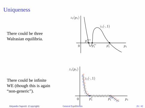
Uniqueness

There could be threeWalrasian equilibria.

p1

z1(p1)

0 p∗

1

z1(·, 1)

p∗∗

1

p∗∗∗

1

There could be infiniteWE (though this is again“non-generic”).

p1

z1(p1)

0 p∗

1

z1(·, 1)

p∗∗

1


Uniqueness

It seems (and can be formally shown) that:

◮ WE areglobally non-unique(generically).

◮ WE arelocally unique(generically).

◮ There are afinite number of WE(generically).

◮ There are anodd number of WE(generically).


Equilibrium and the core

Do competitive markets exhaust all of the gains from trade?

We said that a Walrasian equilibrium requires individual optimality, whichtranslates into the well known condition

− MRSiℓ,k(x

i) =pℓ

pkfor all ℓ 6= k and alli = 1, . . . , I . (2)

Hence, since all individuals face the same prices, (2) implies that

MRSiℓ,k(x

i) = MRSjℓ,k(x

j) for all ℓ 6= k and alli 6= j. (3)

Walrasian equilibrium involves tangency between consumers’ indifferencecurves through their demanded bundles, as illustrated in Fig. 6.

Thus, for an exchange economyE = (ui , ei)Ii=1 satisfying the assumptions of

Theorem 1,every Walrasian equilibrium allocation is in the core.


Equilibrium and efficiencyIf we denote byW(e) the set of Walrasian equilibrium allocationsx(p∗) = (x1(p∗, y1(p∗)), . . . , xI (p∗, yI (p∗))), then,

Theorem 2For an exchange economyE = (ui , ei)I

i=1 satisfying the assumptions ofTheorem 1, W(e) ⊂ C(e).

And we also get the following two results:

Corollary 1 (Nonemptiness of the core)For an exchange economyE = (ui , ei)I

i=1 satisfying the assumptions ofTheorem 1,C(e) 6= ∅.

Theorem 3 (First Welfare Theorem (FWT))Under the hypotheses of Theorem 1, every Walrasian equilibrium allocationx(p∗) is Pareto efficient.


Equilibrium and efficiency

The FWT guarantees that a competitive economy will exhaust all of the gainsfrom trade: a market mechanism, with each agent seeking to maximize hisown utility, results in a PE allocation. That was Adam Smith’s conjecture!

FWT says nothing about the distribution of economic benefits. That is,aWalrasian equilibrium allocation might not be a ‘fair’ or desirable allocation.

Having said that, note that in a market economy Pareto efficiency is achievedwithout demanding much information:each consumer needs to know only hisown preferences and endowments and the market prices.

The fact that competitive markets economize on the use of information in theway just described is a strong argument in favor of using themto allocatescarce resources.


Efficiency and equilibriumWhat about the converse of FWT?

That is, given a Pareto efficient allocation, can we find prices such that thoseprices and the resulting allocation constitute a Walrasianequilibrium?

It turns out that, under certain conditions, the answer is yes.

The intuition is the following:

◮ Pick any PE allocation, sayz;

◮ The indifference curves are tangent atz;

◮ Draw a straight line representing the common slope;

◮ Suppose now the initial endowments are reallocate such thatthe straightline denotes the budget constraint;

◮ The individual’s demands associated to that budget line constitute a WEthat coincides with the initial PE allocationz.


Efficiency and equilibrium

0

0

A

0

0

B

xA1

xA2

xB1

xB2

eA1

eB2

eB1

eA2

zA1

zB2

zB1

zA2

z

e

−p1p2

There exists astraight ‘budget’line separating thetwo ‘uppercounter’ sets atz.

The line connectspointseandzandhas a slope of−p1/p2.


Efficiency and equilibriumIs it always possible the construction of such budget line?

Unfortunately, the answer is no.

In the graph,X is PE, but at the budget line that is tangent to the indifferencecurves atX, agentA demandsY and agentB demandsX, so demand doesn’tequal supply at these prices.



This observation gives us theSecond Welfare Theorem (SWT).

Theorem 4 (Second Welfare Theorem (SWT))Suppose an exchange economyE = (ui , ei)I

i=1 satisfies the assumptions ofTheorem 1. If z∈ F(e) is Pareto efficient, then z is a Walrasian equilibriumallocation for some Walrasian equilibrium prices p∗ after redistribution ofinitial endowments to any allocation e∗ ∈ F(e), such that p∗ · e∗i = p∗ · zi .

SWT says that if all agents have convex preferences, there exists a set ofprices such that every PE allocation is a WE for an appropriate redistributionof the initial endowments.

SWT implies the problems ofdistribution and efficiency can be separated.

Whatever PE allocation we wish to achieve can be implementedby the marketmechanism, i.e.,markets are distributionally neutral.



Prices play two roles in the market system:

1. Allocate role: they indicate (signal) the relative scarcity of the goods.

2. Distributive role: they determine the value of the initial endowments,thereby how much of the different goods each agent can affort.

SWT tells us these two roles can be separated: endowments canberedistributed, and then prices can be used to indicate relative scarcity.

In fact, what is needed is to transfer thepurchasing power of the physicalendowments, which can be done using nondistortionary (lump-sum) taxesthatdon’t depend on economic agents’ choices.


General equilibrium with production

Reference:Jehle and Reny,Advanced Microeconomic Theory, 3rd ed.,Pearson 2011: Ch. 5.

The important properties of competitive markets saw beforecontinue to hold.

However, production brings with it new matters:

◮ Firms’ profits must be distributed back to the consumers who own thefirms.

◮ Distinction between inputs and outputs become obscure whenwe viewthe production size of the economy as a whole (an input for onefirmmight be an output for another).


EconomyThe economy is made of (i)j = 1, . . . , J firms; (ii) i = 1, . . . , I consumers;and (iii) k = 1, . . . , N goods.

Each firmj possesses aproduction possibility setYj.

Assumption 1

◮ 0 ∈ Yj ⊆ RN.

◮ Profits are bounded from below by zero.

◮ Yj is closed and bounded.

◮ Single-value and continues output supply and input demand functions.

◮ Yj strongly convex: for ally, y′ ∈ Yj , there existsy ∈ Yj such thaty ≥ αy + (1− α)y′ for all α ∈ (0, 1).

◮ Rules out constant and increasing returns to scale; ensuresprofitmaximizer is unique.


Producers

A production planfor firm j is a vectoryj ∈ Yj, with the convention thatyj

k < 0 (resp.yjk > 0) if goodk is an input (resp. an output) forj.

Given a nonnegative price vectorp ∈ RN+, each firmj solves theprofit

maximization problem (PMP)

maxyj∈Yj

p · yj . (4)

◮ The objective function is continuous.

◮ The constraint set is bounded and closed.

◮ By the Weierstrass Theorem, a maximum always exists.

For all p ∈ RN+, let Πj(p) ≡ max

yj∈Yjp · yj be firm’s j profit function.


ConsumersEach individuali = 1, . . . , I is endowed by nature with

◮ A certain (nonnegative) amountei = (ei1, . . . , ei

N) ∈ RN+ of each good;

◮ A continuous, increasing and quasiconcave utility function ui : RN+ → R;

◮ A fraction (share) 0≤ θij ≤ 1 of firm j’s profits, with

I∑

i=1

θij = 1 for all j.

For anyp ≥ 0, letmi(p) = p · ei +∑J

j=1 θij Πj(p) be consumeri’s income. Inthis economy with production and private ownership of firms,consumeri’sutility maximization problem (UMP)is

maxxi∈Bi(p)

ui(xi), (5)

whereBi(p) ≡ {xi ∈ RN+ : p · xi ≤ mi(p)} denotes consumeri’s budget set.


EquilibriumDenote byyj(p) andxi(p, mi(p)) the solutions of (4) and (5), respectively.

Theaggregate excess demand function in marketk is

zk(p) =I

∑

i=1

xik(p, mi(p)) −

J∑

j=1

yjk(p) −

I∑

i=1

eik, (6)

and theaggregate excess demand vectoris

z(p) = (z1(p), . . . , zN(p)). (7)

A Walrasian equilibriumfor the economyE = (ui , ei , θij , Yj) is a price vectorp∗ ∈ R

N+ such thatz(p∗) = 0.

Theorem 5 (Equilibrium existence with production)Consider the economyE = (ui , ei , θij , Yj), where each ui and Yj satisfy theassumptions made above and y+

∑Ii=1 ei ≫ 0 for some aggregate production

vector y∈∑J

j=1 Yj. Then there exists a price system p∗ ∈ RN+ for E such that

z(p∗) = 0.Alejandro Saporiti (Copyright) General Equilibrium 40 / 42

Welfare

An allocation(x, y) = (x1, . . . , xI , y1, . . . , yJ) is feasibleif xi ∈ RN+ for all i,

yj ∈ Yj for all j, andI

∑

i=1

xi =

I∑

i=1

ei +

J∑

j=1

yj . (8)

Definition 7 (Pareto efficiency with production)A feasible allocation(x, y) is said to bePareto efficient (PE)if there is noother feasible allocation(x, y) such thatui(xi) ≥ ui(xi) for all i = 1, . . . , I ,with strict inequality for somei.

Theorem 6 (First Welfare Theorem with production)If each ui is strictly increasing onRn

+, then every Walrasian equilibriumallocation (x, y) is Pareto efficient.


Welfare

Theorem 7 (Second Welfare Theorem with production)Suppose the economyE = (ui , ei , θij , Yj) satisfies the following assumptions:

1. ui is a continuous, increasing and quasiconcave;

2. Yj verifies Assumption 1;

3.∑I

i=1 ei +∑J

j=1 yj ≫ 0 for some(y1, . . . , yJ).

If (x, y) is a Pareto efficient allocation, then there are (i) income transfersT1, . . . , TI , with

∑Ii=1 Ti = 0, and (ii) a price vectorp ∈ R

N+ such that:

◮ For all i = 1, . . . , I, xi maximizes ui(xi) subject top · xi ≤ mi(p) + Ti;

◮ For all j = 1, . . . , J, yj maximizesp · yj subject to yj ∈ Yj.


Notes on General Equilibrium - personalpages.manchester.ac.uk · Reference: Jehle and Reny, Advanced Microeconomic Theory, 3rd ed., Pearson 2011: Ch. 5. Behind the superﬁcial chaos

Documents