Northeastern Chukchi Sea demersal fishes and associated environmental characteristics, 2009–2010

Continental Shelf Research 67 (2013) 77–95

Contents lists available at ScienceDirect

Continental Shelf Research

0278-43http://d

$ThisCommomits nothe orig

n CorrE-m

(S.W. Ra(B.J. Galleedenfi

journal homepage: www.elsevier.com/locate/csr

Research papers

Northeastern Chukchi Sea demersal fishes and associatedenvironmental characteristics, 2009–2010$

Brenda L. Norcross a,n, Scott W. Raborn b, Brenda A. Holladay a, Benny J. Gallaway b, StephenT. Crawford c, Justin T. Priest c, Lorena E. Edenfield a, Robert Meyer b

a Institute of Marine Science, School of Fisheries and Oceans, University of Alaska, Fairbanks, AK 99775-7220, USAb LGL Ecological Research Associates, Inc., 1410 Cavitt Street, Bryan, TX 77801, USAc LGL Alaska Research Associates, Inc., #C1-2000 W International Airport Rd., Anchorage, AK 99502, USA

a r t i c l e i n f o

Article history:Received 7 December 2012Received in revised form14 May 2013Accepted 16 May 2013Available online 11 June 2013

Keywords:AlaskaDemersal fish communitySpecies richnessArctic codArctic staghorn sculpinBering flounder

43/$ - see front matter & 2013 The Authors. Px.doi.org/10.1016/j.csr.2013.05.010

is an open-access article distributed undens Attribution-NonCommercial-No Derivativen-commercial use, distribution, and reproductinal author and source are credited.esponding author. Tel.: +1 907 474 7990; fax:ail addresses: [email protected] (B.L. Norcborn), [email protected] (B.A. Holladay)laway), [email protected] (S.T. Crawford), [email protected] (L.E. Edenfield), rmmeyer@att

a b s t r a c t

Three closely-spaced study areas in the northeastern Chukchi Sea off of Alaska provided a opportunity toexamine demersal fish communities over a small spatial scale as part of a multidisciplinary program.During 2009 and 2010, fishes in the three study areas (Klondike, Burger, and Statoil) were sampled at 37stations with a plumb staff beam trawl and a 3 m beam trawl; 70% of stations were sampled during allthree cruises. Fish catches were dominated by small fishes (o150 mm TL), which cannot be whollyattributed to the small mesh size of the net. Output from generalized linear modeling of the datasuggested that overall fish density, species richness, and density of Arctic staghorn sculpin (Gymno-canthus tricuspis) and Bering flounder (Hippoglossoides robustus) were higher in the more southerlyKlondike study area than in the more northerly Burger and Statoil study areas. Arctic cod (Boreogadussaida) was abundant throughout the study region. Richness and density could be explained by theenvironmental variables that defined the overall study area. The Klondike study area was warmer anderosional in nature with higher proportions of gravel sediment. Other study areas were colder and moredepositional in nature with muddier sediment and were characterized by high densities of megafaunalinvertebrates such as brittle stars. There appeared to be a lack of ecological homogeneity across thesethree closely-spaced study areas of the Chukchi Sea.

& 2013 The Authors. Published by Elsevier Ltd. All rights reserved.

1. Introduction

Baseline information about offshore ecosystems in the north-eastern Chukchi Sea in general, and arctic marine fishes inparticular, is sparse (Johnson, 1997; Power, 1997; Mecklenburget al., 2002, 2008). There are no commercial fisheries in federalwaters of the Alaskan arctic (Zeller et al., 2011), so baseline datacannot be reconstructed using historical commercial fisheriesharvest data. At present, commercial fisheries for demersal fishesare prohibited in this area (North Pacific Fisheries ManagementCouncil (NPFMC), 2009), and mostly subsistence fishing in theregion is limited to large pelagic fishes taken close to shore.

The entire Chukchi Sea is north of the regular fish-trawl researchsurveys conducted by NOAA Fisheries. Knowledge of the demersal

ublished by Elsevier Ltd. All rights

r the terms of the CreativeWorks License, which per-

ion in any medium, provided

+1 907 474 1943.ross), [email protected], [email protected]@lgl.com (J.T. Priest),.net (R. Meyer).

fish communities in the Chukchi Sea comes from 23 scientificcruises in the eastern Chukchi Sea from 1959 to 2008. Since 1973, 16cruises have collected fishes in the northeast Chukchi Sea at somestations north of 701N. Unfortunately, these investigations used 15different types of demersal trawls with headropes ranging from 3 mto 43 m and smallest mesh between 4 mm and 90 mm, whichprohibits quantitative comparisons across studies (Norcross et al.,2013). The fishing gear used affects the number of fishes captured,however, the dominant fishes in the catch were comparablebetween recent (2004–2008; Norcross et al., 2013) and historical(1990–1991; Barber et al., 1997) collections. Over time Arctic cod(Boreogadus saida) was the most abundant demersal (Alverson andWilimovsky, 1966; Frost and Lowry, 1983; Barber et al., 1997) andpelagic (Eisner et al., 2013) species. The same fish families domi-nated the northeast Chukchi throughout the historical collections(Norcross et al., 2013): cods (Gadidae), sculpins (Cottidae), eelpouts(Zoarcidae), and righteye flounders (Pleuronectidae).

Potential oil and gas exploration in US waters off Alaska hasprompted interest in the overall ecology of the northeastern ChukchiSea. The Chukchi is a shallow sea in the arctic bordered on the east bythe Beaufort Sea and Alaskan coast, on the north by the Arctic Ocean,and on the south by the Bering Strait. Waters flow northward intothe Chukchi Sea from the Bering Sea through Bering Strait. Renewedinterest in this area provides the opportunity to fill longstanding gaps

reserved.

B.L. Norcross et al. / Continental Shelf Research 67 (2013) 77–9578

in understanding of the fish communities of the region. The ChukchiSea Environmental Studies Program (CSESP) is an industry-sponsored comprehensive study (summarized by Day et al., 2013)focused around prospective development of three blocks (henceforthreferred to as study areas) offshore in the Chukchi Sea (Fig. 1). Eachstudy area has leases permitted to different companies with theirown schedules for exploration. As such, the three study areas mayexperience differences with respect to the timing and severity ofpotential disturbances due to oil and gas development. Althoughthere is nothing biologically significant about the boundaries circum-scribing each study area, they represent logical partitions towards thefacilitation of defining future disturbances and quantifying theireffects.

Therefore our primary objective was to examine abundance ofdemersal fishes over the three closely-spaced study areas in thenortheast Chukchi Sea by estimating and comparing descriptors ofthe fish community. Descriptors included species richness, total

Fig. 1. Three study areas and stations sampled for fish in the northeastern Chukchi Sea,is shown (modified from Weingartner et al., 2008).

density, assemblage structure, and densities of five selectedspecies, each of which represents a prominent family of fishes:Arctic cod (B. saida), Arctic staghorn sculpin (Gymnocanthus tricuspis),Canadian eelpout (Lycodes polaris), stout eelblenny (Anisarchus med-ius), and Bering flounder (Hippoglossoides robustus). Our initialexpectation was that there would be little, if any, difference in thefish communities given their proximity.

Detecting changes in fish abundances can be confounded byenvironmental factors across space and time. Physical gradientsare known to affect Chukchi fish communities over hundreds ofkilometers (Barber et al., 1997; Norcross et al., 2011a, 2011b, 2013),but nothing is known about the effect over smaller spatial scales.Therefore our second objective was to relate any changes in thefish descriptor variables, if present, to physical gradients over thesmall, closely-spaced study areas.

Our third objective was to test for differences between two verysimilar types of trawls that were used in 2010. Examination of

2009–2010. The generalized direction of water flow in the indicated water masses

B.L. Norcross et al. / Continental Shelf Research 67 (2013) 77–95 79

historical fish data from the Chukchi Sea concluded that charac-terization of the demersal fish community was dependent upontype of gear used for collections (Norcross et al., 2013). Therefore,we examined catch differences between two gears whose efficien-cies may have varied across species.

2. Study areas and methods

2.1. At-sea sampling

Three cruises in the northeastern Chukchi Sea contributed tothe field collections made during this study: 23 July–18 August2009, 22 September–12 October 2009, and 28 August–19 Septem-ber 2010. We sampled two study areas (Klondike and Burger)during each of the 2009–2010 cruises and added a third area,Statoil, in 2010 (Fig. 1). Fish sampling occurred at predeterminedstations arranged in a systematic, fixed grid within each studyarea. The Klondike and Burger study areas were identical in shapeand size at ∼55.6�∼55.6 km (30�30 NM; Fig. 1). These two studyareas were non-adjacent and centered about 70 km apart; thenortheastern corner of Klondike was about 26 km from the south-western corner of Burger. The Statoil study area was irregularlyshaped, but covered about the same area (∼3100 km2) as each ofthe other two study areas, and adjoined the northwestern edge ofthe Burger study area. Stations were laid out in a grid with∼13.75 km (7.5 NM) spacing; Klondike and Burger each had 13fixed stations and Statoil had 11 stations.

Environmental characteristics at each fish sampling stationwere assessed by other researchers of the CSESP. Vertical casts ofa conductivity temperature density (CTD) instrument were con-ducted to assess bottom-water characteristics (Weingartner et al.,2013). Percent gravel, sand, and mud were assessed from sedimentcollected with a van Veen grab at each fishing station (Blanchardet al., this 2013a).

A 3 m plumb staff beam trawl (PSBT), modified from Gundersonand Ellis (1986), was used to collect demersal fishes in 2009 and2010. Modifications included shortening the beam from 3.66 m to3.05 m, seizing a lead-filled line to the foot rope and attaching15 cm lengths of chain at 15 cm intervals along the foot rope, andlengthening the codend from 1 m to 4 m (Norcross et al., 2011a,2011b). The net was rigged with a double tickler chain thatconsisted of a chain that was 0.5 m shorter than the foot rope anda second that was 0.9 m shorter than the foot rope. The effectivemouth opening was 2.26�1.20 m. The net was 7 mm woven nylonnetting with a 4 mm mesh codend liner. The PSBT was towed ato2 kt on the bottom for ∼3–5 min in 2009 and ∼2–3 min in 2010,although there were instances in both years when it was towed for410 min. The PSBT was efficient at sampling the demersal fishcommunity (Norcross et al., 1995), but was prone to fill withinvertebrates and sediment, which limited the efficiency of proces-sing tows of longer durations. The length of wire deployed wasusually 2.5–3.5 times water depth. Bottom time was from whentowing cable was completely deployed to start of haul back.

In tandem with fishing the PSBT, during 2010 we also fished atrawl that was designed to limit invertebrate and sedimentaccumulation at each station. The 3 m model 38 skate beam trawl(3mBT) consisted of a 5 m model 38 Skate Trawl fitted to a 3 mlong tubular steel beam. The 3mBT had a 5 m head rope and a 6 mfoot rope with 9 m of chain attached to the foot rope. The net wasoutfitted with a 12 mm mesh codend liner. To help keep the footrope from digging into the bottom, the foot rope was equippedwith 10 cm foam rollers. The vertical opening of the net was 1.0–1.5 m. The wing ends of the net were attached directly to the 3 mbeam. The 3mBT was much less prone to filling with invertebrates

and sediment than the PSBT, which allowed for tow times to be15–30 min at o2 kt.

Fish sampling was conducted aboard the 58 m long R/V West-ward Wind, a converted king crab fishing and processing vessel.Gear deployment was limited to aft of the forecastle using a ship-mounted deck crane and a single trawl winch. Drag caused by thetrawl and the forward location of the towing point caused the shipto slew to the right, which resulted in a curved tow track. Starttime began when the appropriate amount of tow cable wasdeployed and stopped when retrieval of the cable began. Towingdistance for each haul was calculated as a cumulative distancebetween each 10-s increment of tow time. The distance towed wasmultiplied by the width of the net mouth to get area fished at eachstation. This likely underestimated area sampled as the nets likelycontacted the bottom before all of the tow cable was paid out.On one occasion during the August 2009 cruise, the PSBT catchwas too large to bring aboard safely; approximately half of thehaul was discarded overboard. To compensate, the catch quanti-fied from half of the haul was doubled for this station.

At sea fishes were provisionally identified to the most specifictaxonomic level possible using available guides (Matarese et al.,1989; Mecklenburg et al., 2002), counted and measured. Inverte-brates in these collections are reported elsewhere (Blanchard et al.,2013b). A subsample of each species was subsequently examinedonshore and identifications were finalized. Nomenclature followsthe American Fisheries Society's publication of scientific andcommon names (Nelson et al., 2004) except for those speciesrecognized after that publication (Mecklenburg et al., 2011). Whena fish was broken into multiple pieces, only the head was countedto avoid duplicate counts. Total length (TL) of fishes was measuredto the nearest mm.

2.2. Statistical methods for the univariate descriptors of the fishcommunity

Dependent variables (i.e., univariate descriptors) included Spe-cies richness, Total fish density, and the numerical densities of Arcticcod, Arctic staghorn sculpin, Canadian eelpout, stout eelblenny andBering flounder. By modeling Species richness on a per-1000 m2

basis we could control for continuous increasing of richness withfishing effort (e.g., Lobo and Martin-Piera, 2002; O'Hara, 2005).Density values were reported per 1000 m2. Objective 1 was toassess the inherent differences in these variables across the studyareas and years. The model for Objective 1 was termed theenvironmentally naive (EN) model because no environmental datawere included. The only independent variables were categorical:Study Area, Year, and Gear. Gear accounted for sampling efficiencyvarying between the two trawl types (Objective 3).

An environmentally informed (EI) model addressed Objective 2.In addition to the three categorical variables in the EN model, eightcontinuous variables were added to the EI model: Depth, Bottomtemperature, Bottom salinity, Percent gravel in the substrate, Percentmud in the substrate, Latitude (north), Longitude (east), and Distanceoffshore. Percent sand was measured also but only two of thesubstrate variables were needed because the three types summedto 100%. Sand and mud were the most strongly inversely correlated,so we omitted Percent sand to reduce multi-collinearity.

Effect size across levels of the categorical variables for both ENand EI models was determined by comparing marginal means.These means were output from generalized linear models (GLMs),which corrected for missing factor combinations and unbalanceddesigns to give equal weight to all levels of all other categoricalvariables. Marginal means for categorical variables in the EI modelassumed values for the continuous variables were equal to theirobserved averages across all samples.

Table 1Density of fishes captured by 3 m plumb staff beam trawl (PSBT) in the northeastern Chukchi Sea, by study area, 2009–2010. Catch is adjusted to count of fish per 1000 m2, and averaged over hauls in the stratum. Species list isbased on both types of benthic trawl collections combined. Dashes indicate zero catches.

Scientific and common names Study area Over all hauls

Klondike Burger Statoil Mean % Of

Jul/Aug 2009 Sep/Oct 2009 Aug/Sep 2010 Mean Jul/Aug 2009 Sep/Oct 2009 Aug/Sep 2010 Mean Aug/Sep 2010 density total fish densityGadidae (Cods)Boreogadus saida 52.2 23.3 62.1 45.8 19.1 52.1 27.2 33.2 15.6 36.6 32.50%

Arctic codTheragra chalcogramma – – – – – 0.2 – o0.1 – o0.1 o0.1%Walleye pollockCottidae (Sculpins)Artediellus scaber 17.5 14.3 7 12.9 20.2 2.1 2.6 8 1.3 9.3 8.30%

HameconGymnocanthus tricuspis 6.4 19.4 8.4 11.4 0.9 0.1 0.6 0.5 – 5.3 4.70%

Arctic staghorn sculpinHemilepidotus papilio 0.1 – – o0.1 – – – – – o0.1 o0.1%

Butterfly sculpinIcelus spatula – 1.4 – 0.5 2.5 0.2 3.3 2 – 1.1 0.9%

Spatulate sculpinMyoxocephalus scorpius 5.6 41.6 14.3 20.5 1 4 2.1 2.4 0.6 10.2 9.1%

Shorthorn sculpinTrichocottus brashnikovi – 0.2 – o0.1 – – – – – o0.1 o0.1%

Hairhead sculpinTriglops pingelii 0.3 1.4 0.5 0.7 – 0.4 – 0.1 – 0.4 0.3%

Ribbed sculpinHemitripteridae (Sailfin sculpins)Nautichthys pribilovius 0.1 0.9 – 0.4 – – – – 0.4 0.2 0.2%

Eyeshade sculpinAgonidae (Poachers)Aspidophoroides monopterygius 0.4 0.7 0.3 0.5 – – – – – 0.2 0.20%

AlligatorfishHypsagonus quadricornis – – 0.2 o0.1 – – – – – o0.1 o0.1%

Fourhorn poacherUlcina olrikii 1.9 2.6 2.2 2.2 1.3 0.7 2.3 1.4 1.5 1.8 1.6%

Arctic alligatorfishLiparidae (Snailfishes)Liparis bathyarcticus 0.8 1.3 – 0.7 0.3 0.6 – 0.3 – 0.4 0.4%

Nebulous snailfishLiparis tunicatus 0.4 0.3 1.8 0.9 0.3 0.7 1.6 0.9 – 0.8 0.7%

Kelp snailfishZoarcidae (Eelpouts)Gymnelus hemifasciatus 2 0.4 – 0.8 21.7 1.8 7.8 10.1 1.5 4.9 4.4%

Halfbarred poutGymnelus viridis 0.3 1.1 – 0.5 4 1.1 1.5 2.1 0.4 1.2 1.0%

Fish doctorLycodes mucosus 0.2 0.5 – 0.2 – – – – – 0.1 0.1%

Saddled eelpoutLycodes palearis 0.1 0.1 0.2 0.1 – – – – – o0.1 0.1%

Wattled eelpoutLycodes polaris 5.3 1.9 2.9 3.4 15.6 9.2 1.8 8.7 6 6 5.3%

Canadian eelpoutLycodes raridens 1.7 2.5 0.9 1.7 3.4 1.6 2 2.3 2.8 2.1 1.9%

Marbled eelpoutStichaeidae (Pricklebacks)Anisarchus medius 33.9 15.6 4.8 18.1 71.2 16.6 1.6 28.7 1.7 20.6 18.3%

Stout eelblenny

B.L.Norcross

etal./

ContinentalShelf

Research

67(2013)

77–95

80

Eumesog

rammus

prae

cisus

0.4

2.9

–1.1

0.4

––

0.1

–0.5

0.5%

Fourlinesn

akeb

lenny

Leptoclin

usmaculatus

––

––

0.2

––

o0.1

–o

0.1

o0.1%

Dau

bedsh

anny

Lumpe

nusfabricii

16.5

20.1

7.5

14.7

9.7

2.4

0.2

40.4

8.3

7.4%

Slen

der

eelblenny

Sticha

euspu

nctatus

0.1

0.8

0.3

0.4

0.3

––

0.1

–0.2

0.2%

Arcticsh

anny

Ammodytidae

(San

dlance

s)Ammod

ytes

hexa

pterus

–0.9

–0.3

–4.6

–1.6

0.3

0.8

0.8%

Pacificsandlance

Pleuro

nec

tidae

(Righteye

flounders)

Hippo

glossoides

robu

stus

4.2

2.7

1.3

2.7

0.3

––

0.1

–1.2

1.1%

Beringflou

nder

Liman

daprob

oscide

a–

0.2

–o

0.1

––

––

–o

0.1

o0.1%

Longh

eaddab

Totalfish

den

sity—

Mea

n7

StDev

150.37

148.7

156.97

111.0

114.77

116.3

140.67

124.5

172.47

137.0

98.47

34.9

54.57

92.1

106.87

105.4

32.47

26.6

112.57

112.9

100.00%

Cou

ntof

species

2225

1627

1817

1321

1229

Cou

ntof

stations

1313

1339

1213

1338

1188

B.L. Norcross et al. / Continental Shelf Research 67 (2013) 77–95 81

We used GLMs with discrete probability distributions tocompute the likelihood of observing the counts of fish that werecollected. These types of GLMs have become the standardapproach for analyzing catch-per-unit-effort (CPUE) data (Powerand Moser, 1999; Terceiro, 2003; Minami et al., 2007; Arab et al.,2008; Shono, 2008; Raborn et al., 2011). We considered bothPoisson and negative binomial distributions to model theseresponses. Akaike's Information Criterion (AICc; Burnham andAnderson, 2002) was used to determine which of the twodistribution types was most appropriate for the data beingconsidered. It indicated that the negative binomial model wasbest for all response variables.

2.3. Spatial visualization of univariate fish community descriptorsand environmental gradients

Each study area was visually characterized with contour mapsof substrate variables, as well as the aforementioned univariatefish descriptor variables showing significant differences (α¼0.05)across the three areas based on output from the EN model. Spatialcontours of these variables were interpolated using ArcMap© 10software and the spatial analyst extension (ESRI, Inc.). Speciesrichness, Density, and Bottom temperature were interpolated bykriging data and allowing the ArcMap software to assign groupswith natural breaks inherent in the data (Jenks Natural Breaks).Kriging generated an estimated surface from a scattered set ofpoints with z-values; it does not necessarily present the full rangeof recorded data. Substrate data were interpolated with an inversedistance weighted model, which estimated cell values by aver-aging the values of sample data points in the neighborhood of eachprocessing cell; break points were assigned manually at 10%intervals. Contours of Species richness and Density were calculatedusing only the PSBT from collections during 2009 and 2010.Temperature contours were created for each cruise separately;substrate contours were calculated as the average per station of allsubstrate samples examined for grain size, 2008–2010 (data fromBlanchard et al., 2013a).

2.4. Statistical methods for a multivariate descriptor of the fishcommunity

The multivariate response, Assemblage structure, was quantifiedfor each sample by the relative abundances of all species. Therelative abundance of a species is given by the CPUE of the speciesin the sample divided by the total CPUE of all species in thesample; thus, relative abundances for a given sample sum to one.Assemblage structure was analyzed using nonmetric multidimen-sional scaling (nMDS), which is a nonparametric ordinationtechnique based on ranks and is insensitive to zeroes (Manzerand Shepard, 1962; Kruskal, 1964). All ordinations were performedwith the statistical software PC-ORD (McCune and Mefford, 2006).Both axes exhibited p-values less than 0.01 based on comparingobserved stress values with those derived from Monte Carlo runsof randomized data.

The nMDS ordination is an indirect gradient analysis wherebycontinuous variables must be correlated with the station axes posthoc and can be overlaid on the ordination biplot. The resultingbiplot addresses Objective 1 by allowing visualization of thetemporal and spatial variability in Assemblage structure acrossyears and study areas, i.e., the distinctiveness of their respectivefish communities. Towards addressing Objective 2, overlayingenvironmental variables with the station axis scores delineateshow variability in assemblage structure correlated with thesevariables, which may indicate important environmental forcingof community dynamics. The biplot also can be used to determineif samples grouped by gear type (Objective 3).

Table 2Density of fishes captured by 3 m beam trawl (3mBT) in the northeastern Chukchi Sea, by study area, 2010. Catch is adjusted to count of fish per 1000 m2, and averaged overhauls in the stratum. Species list is based on both types of benthic trawl collections combined. Dashes indicate zero catches.

Study area Over all hauls

KlondikeAug/Sep

BurgerAug/Sep

StatoilAug/Sep

Mean density % Of total fish

Scientific and common names 2010 2010 2010 densityGadidae (Cods)B. saida 4.7 3.1 3.5 3.6 41.3%

Arctic codT. chalcogramma – – – – –

Walleye pollockCottidae (Sculpins)A. scaber 5.7 0.2 o0.1 1.3 14.7%

HameconG. tricuspis 2.7 o0.1 – 0.6 6.5%

Arctic staghorn sculpinH. papilio – – – – –

Butterfly sculpinI. spatula – o0.1 o0.1 o0.1 0.6%

Spatulate sculpinM. scorpius 1.6 o0.1 o0.1 0.4 4.3%

Shorthorn sculpinT. brashnikovi o0.1 – – o0.1 0.1%

Hairhead sculpinT. pingelii 0.3 o0.1 o0.1 o0.1 1.0%

Ribbed sculpinHemitripteridae (Sailfin sculpins)N. pribilovius 1.5 – – 0.3 3.4%

Eyeshade sculpinAgonidae (Poachers)A. monopterygius – – – – –

AlligatorfishH. quadricornis 0.1 – – o0.1 0.3%

Fourhorn poacherU. olrikii 0.8 0.2 0.1 0.3 3.1%

Arctic alligatorfishLiparidae (Snailfishes)L. bathyarcticus – – o0.1 o0.1 0.1%

Nebulous snailfishL. tunicatus 0.4 o0.1 o0.1 0.1 1.7%

Kelp snailfishZoarcidae (Eelpouts)G. hemifasciatus 0.1 0.1 – o0.1 0.9%

Halfbarred poutG. viridis o0.1 o0.1 – o0.1 0.6%

Fish doctorL. mucosus – – – – –

Saddled eelpoutL. palearis – – – – –

Wattled eelpoutL. polaris 0.3 1.0 0.4 0.6 7.1%

Canadian eelpoutL. raridens 0.4 0.3 0.1 0.2 2.6%

Marbled eelpoutStichaeidae (Pricklebacks)A. medius 0.5 0.9 0.4 0.6 7.0%

Stout eelblennyE. praecisus 0.4 o0.1 – o0.1 1.0%

Fourline snakeblennyL. maculatus – – – – –

Daubed shannyL. fabricii 0.6 0.2 o0.1 0.2 2.6%

Slender eelblennyS. punctatus 0.2 – – o0.1 0.5%

Arctic shannyAmmodytidae (Sand lances)A. hexapterus o0.1 – – o0.1 0.1%

Pacific sand lancePleuronectidae (Righteye flounders)H. robustus o0.1 o0.1 o0.1 o0.1 0.5%

Bering flounderL. proboscidea – – – – –

Longhead dabTotal fish density—Mean7St Dev 20.5713.8 6.376.0 4.975.9 8.779.8 100.0%Count of species 20 16 13 23Count of stations 6 13 11 30

B.L. Norcross et al. / Continental Shelf Research 67 (2013) 77–9582

B.L. Norcross et al. / Continental Shelf Research 67 (2013) 77–95 83

Sampling across factor combinations was unbalanced andmissing altogether for some combinations; the 3mBT was usedonly in 2010, and Statoil was sampled only in 2010. The nMDSordination cannot correct for missing factor combinations orunbalanced sampling; therefore, any differences in how samplesfrom a given categorical variable group together in the ordinationbiplot may be confounded by influences from other variables. ForGLMs the multivariate Assemblage structure was reduced to twounivariate descriptors, axis 1 and axis 2, which are the coordinatesthat position samples in the ordination biplot. Similar approacheshave been used successfully to assess assemblage structures ofother systems (Matthews, 1987; Gelwick, 1990; Raborn et al.,2001). The GLMs correct for imbalances and fill in missing datato isolate the effect of each categorical variable on the “average”Assemblage structure. We assumed axis 1 and axis 2 were normallydistributed when parameterizing their GLMs.

3. Results

3.1. Effort and catch summaries

In total, 37 distinct stations were trawled 2–4 times during thisstudy (Fig. 1). These stations were systematically spaced in each ofthe study areas: 13 in Klondike, 13 in Burger, and 11 in Statoil.All effort totaled 161,316 m2 of bottom sampled with the twodemersal trawl types. The majority of this total area was sampledwith the 3mBT in 2010 because it was deployed for ∼15–30 minduring each tow as opposed to the ∼3–5 min tow durations withthe PSBT.

A total of 29 species were represented in the combined demersaltrawl collections (Tables 1 and 2). The 10 most abundant species inthe PSBT and 3mBT collections made up 93% and 90% of the totalcatch, respectively. In order of overall abundance, those specieswere Arctic cod, stout eelblenny, shorthorn sculpin (Myoxocephalusscorpius), hamecon (Artediellus scaber), slender eelblenny (Lumpenusfabricii), Canadian eelpout, Arctic staghorn sculpin, halfbarred pout

Table 3Predicted responses of categorical variables from the environmentally naive (EN) and enortheastern Chukchi Sea. Predicted marginal mean values (the means that are estimateas density of fish, i.e., count per 1000 m2. Models are based on 2009–2010 collections w

Predicted marginal mean Study area

Klondike Burger Statoil p

Environmentally naive modelSpecies richness 4.97 5.09 3.383 0.032Total fish density 50.36 30.13 18.59 o0.001Arctic cod 15.23 10.82 8.61 0.219Arctic staghorn sculpin 5.33 0.17 o0.01 o0.001Canadian eelpout 1.12 2.74 2.10 0.043Stout eelblenny 4.33 5.38 2.56 0.294Bering flounder 0.74 0.03 0.24 0.001Assemblage structure

nMDS axis 1 −0.02 0.082 −0.052 0.593nMDS axis 2 0.35 −0.171 −0.491 o0.001

Environmentally informed modelSpecies richness 4.79 4.48 4.30 0.926Total fish density 38.07 31.12 19.00 0.306Arctic cod 12.88 11.33 6.42 0.460Arctic staghorn sculpin 0.30 0.34 o0.01 0.994Canadian eelpout 2.47 1.56 0.20 0.024Stout eelblenny 7.57 3.95 0.50 0.013Bering flounder 0.29 0.07 0.06 0.425Assemblage structure

nMDS axis 1 0.315 −0.073 −0.485 0.057nMDS axis 2 −0.053 −0.033 −0.009 0.988

(Gymnelus hemifasciatus), marbled eelpout (Lycodes raridens), andArctic alligatorfish (Ulcina olrikii). Of the five most abundant speciescollected for each trawl type, three species were common to bothlists: Arctic cod, hamecon, and stout eelblenny. Eight species ofsculpins were captured by each gear type, which is more than forany other fish family occurring in the study area (Tables 1 and 2).Arctic cod was the dominant taxon caught by both trawls, compos-ing 33% of the PSBT and 41% of the 3mBT collections.

Overall, both the total density of fishes caught and the numberof species taken in both types of demersal trawls were highest inthe more southerly Klondike study area and were much lower inthe more northerly Burger and Statoil study areas. In the 2009PSBT collections for Klondike (Table 1), total fish densities weresimilar in July/August and September/October 2009, and approxi-mately 25% lower in August/September 2010 (151, 157 and 115 fishper 1000 m2, respectively). Likewise, the Klondike collections inJuly/August and September/October 2009 caught more speciesthan were caught in August/September 2010 (22, 25, and 16species, respectively). In the PSBT collections from Burger, totalfish densities declined from a peak in July/August 2009 byapproximately 40% in September/October 2009, and by 70% inAugust/September 2010 (173, 98, and 55 fish per 1000 m2, respec-tively). Similar to Klondike, higher numbers of species were caughtin Burger during July/August and September/October 2009 than inAugust/September 2010 (18, 17, and 13 species, respectively).Though the density and number of species in the 2010 PSBTcollections were low in Klondike and Burger, they were even lowerin Statoil with only 32 fish per 1000 m2 and 12 species captured(Table 1). In August/September 2010 the 3mBT total fish densitywas 3–4 times higher in Klondike than in Burger or Statoil (21, 6,and 5 fish per 1000 m2, respectively). The number of speciescaptured in Klondike was highest, with fewer species caught inBurger and fewer still caught in Statoil (20, 16, and 13 species,respectively).

The demersal trawl collections were dominated numerically bysmall fishes. Of the 27 species captured by the PSBT, the maximumsizes of 10 species were o100 mm, of 11 species were 100–149mm,

nvironmentally informed (EI) generalized linear models of demersal fishes in thed while holding all other variables constant) are reported for each response variableith both bottom trawl gears.

Year Gear

2009 2010 p PSBT 3mBT p

4.46 4.35 0.836 14.20 1.37 o0.00142.36 21.88 0.001 81.38 11.39 o0.00111.34 11.13 0.945 32.26 3.91 o0.0010.01 o0.01 0.632 0.01 o0.01 0.0322.63 1.32 0.094 5.00 0.69 o0.001

12.28 1.24 o0.001 8.43 1.81 o0.0010.31 0.11 0.041 0.48 0.07 0.012

0.202 −0.193 0.003 0.023 −0.014 0.798−0.033 −0.173 0.245 −0.039 −0.167 0.327

4.67 4.37 0.76 14.86 1.37 0.00143.70 18.24 0.035 82.92 9.61 o0.00116.25 5.89 0.055 27.17 3.52 o0.0010.01 o0.01 0.627 0.01 o0.01 0.0020.84 1.02 0.828 2.26 0.38 o0.0016.91 0.88 0.016 4.79 1.27 0.0020.09 0.13 0.715 0.21 0.05 0.052

−0.055 −0.106 0.858 −0.090 −0.072 0.8980.020 −0.084 0.672 0.061 −0.125 0.128

B.L. Norcross et al. / Continental Shelf Research 67 (2013) 77–9584

of 3 species were 150–199 mm, and of only 3 fish species were4200 mm. The largest fish taken in the PSBT collection was a225 mm TL marbled eelpout (L. raridens) taken in Klondike duringAugust/September 2010. The maximum sizes of the 23 species takenin the 3mBT were similar to those of the PSBT: 10 species wereo100 mm, 9 species were 100–149 mm, 1 species was 150–199 mm,and 3 species were 4200 mm. A 250 mm TL shorthorn sculpincollected in Klondike in August/September 2010 was the largest fishtaken in the 3mBT. Captured fishes in mid-shelf area of the ChukchiSea were almost all o150 mm TL.

3.2. Objective 1: Comparison of fish community descriptors acrossstudy areas and years

The EN model detected significant differences (po0.05) amongstudy areas for Species richness, Total fish density, and the densities ofArctic staghorn sculpin, Canadian eelpout, and Bering flounder(Table 3). These estimated fish densities were greatest in the moresoutherly Klondike study area, with the exception of Canadian eelpoutwhich was higher in Burger. Total fish density, stout eelblenny density,and Bering flounder density declined significantly from 2009 to 2010.

The contour maps show the number of species and density offishes to be the highest in Klondike and lowest in Statoil. Species

Fig. 2. Species richness among and within each of the Klondike, Burger and Statoil study2010.

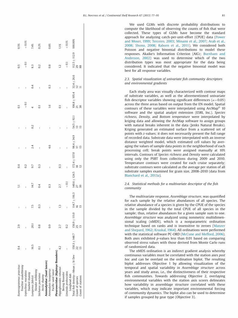
richness was concentrated in the center east of Klondike (Fig. 2). Forboth gears, there were 28 fish species captured in Klondike, 24species in Burger, and 17 species in Statoil (Tables 1 and 2). Up to 21species were captured at one station in Klondike, while as few asthree were caught in Statoil. Total fish density was higher and morehomogenously high throughout Klondike and increased somewhat atthe southern and western edges, but was concentrated towards thecenter of the Burger study area (Fig. 3). Arctic cod was the mostabundant and evenly distributed species, though the density was lowin Statoil (Fig. 4). The southeast corner of Klondike had highconcentrations of Arctic staghorn sculpin, and very few werecaptured in the other two study areas (Fig. 5). Canadian eelpoutwas concentrated in the northwest corner of the Burger study area,overlapping into the southeast corner of Statoil (Fig. 6). Canadianeelpout was almost absent from the southeast part of Klondike. Stouteelblenny had the highest densities in Burger and the lowest in thenorthwest corner of the Statoil study area (Fig. 7). Bering flounderwas found throughout Klondike, especially concentrated in northcentral, and was extremely low in Burger and Statoil (Fig. 8).

Patterns were seen in fish densities between years and amongstudy areas (Fig. 9). Between-year variability could be seen alongthe x-axis (axis 1) of the nMDS ordination biplot, with more 2009collections on the right and 2010 collections on the left. Between

areas based on plumb staff beam trawl collections, northeastern Chukchi Sea 2009–

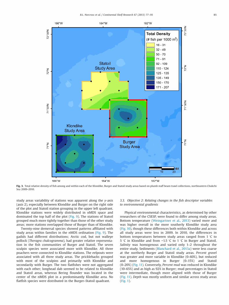
Fig. 3. Total relative density of fish among and within each of the Klondike, Burger and Statoil study areas based on plumb staff beam trawl collections, northeastern ChukchiSea 2009–2010.

B.L. Norcross et al. / Continental Shelf Research 67 (2013) 77–95 85

study areas variability of stations was apparent along the y-axis(axis 2), especially between Klondike and Burger on the right sideof the plot and Statoil station grouping in the upper left quadrant.Klondike stations were widely distributed in nMDS space anddominated the top half of the plot (Fig. 9). The stations of Statoilgrouped much more tightly together than those of the other studyareas; more stations overlapped those of Burger than of Klondike.

Twenty-nine demersal species showed patterns affiliated withstudy areas within families in the nMDS ordination (Fig. 9). Thegadids had different distributions; Arctic cod, but not walleyepollock (Theragra chalcogramma), had greater relative representa-tion in the fish communities of Burger and Statoil. The sevensculpin species were associated more with Klondike. All threepoachers were connected to Klondike stations. The eelpouts wereassociated with all three study areas. The pricklebacks groupedwith most of the sculpins and primarily with Klondike andsecondarily with Burger. The two flatfishes were not aggregatedwith each other; longhead dab seemed to be related to Klondikeand Statoil areas, whereas Bering flounder was located in thecenter of the nMDS plot in a predominantly Klondike area. Noflatfish species were distributed in the Burger–Statoil quadrant.

3.3. Objective 2: Relating changes in the fish descriptor variablesto environmental gradients

Physical environmental characteristics, as determined by otherresearchers of the CSESP, were found to differ among study areas.Bottom temperature (Weingartner et al., 2013) varied more andwas higher overall in the more southerly Klondike study area(Fig. 10), though these differences both within Klondike and acrossall study areas were less in 2009. In 2010, the differences inbottom temperatures between study areas ranged from 1 1C to5 1C in Klondike and from −1.5 1C to 1 1C in Burger and Statoil.Salinity was homogenous and varied only 1–2 throughout theentire study. Sediments (Blanchard et al., 2013a) were less coarseat the northerly Burger and Statoil study areas. Percent gravelwas greater and more variable in Klondike (0–60%), but reducedand more homogenous in Burger (0–15%) and Statoil(0–20%) (Fig. 11). Conversely, Percent mud was reduced in Klondike(10–65%) and as high as 92% in Burger; mud percentages in Statoilwere intermediate, though more aligned with those of Burger(Fig. 11). Depth was mostly uniform and similar across study areas(Fig. 1).

Fig. 4. Relative density of Arctic cod within each of the Klondike, Burger and Statoil study areas based on plumb staff beam trawl collections, northeastern Chukchi Sea2009–2010.

B.L. Norcross et al. / Continental Shelf Research 67 (2013) 77–9586

The study areas oriented with the environmental variables. TheKlondike axis scores tended to correlate more positively with Percentgravel and Salinity and more negatively with North, Percent mud andEast (Fig. 9). The directions of these correlations were reversed forBurger and Statoil; however, two stations in the southern part of theBurger study area were not closely associated with Burger or withKlondike. Statoil was related to Distance offshore.

The EI model results did not directly mimic those of the ENmodel. There were fewer significant differences among study areasdetected with the EI model (Table 3), which suggested that theenvironmental gradients underlying the differences among studyareas detected with the EN model were captured by the variablesincluded in the EI model. While stout eelblenny density stilldiffered, Canadian eelpout density switched from being non-significant in the EN model to significant in the EI model.Individual environmental gradients did not account for differencesacross years as the decline in Total fish density and stout eelblennydensity from 2009 to 2010 remained significant. Furthermore, the2010 decline in Arctic cod density became significant with theEI model.

Output from the EI model showed that environmental variablesdid not affect all fish equally (Table 4). Species richness was

positively correlated to Salinity and Temperature. Arctic cod wasthe only species related to Temperature, and Canadian eelpout wasthe only species correlated with Salinity. Total fish density andArctic staghorn sculpin density were negatively correlated withDepth. Arctic cod density was positively related to Distanceoffshore. Arctic cod and Arctic staghorn sculpin were negativelyassociated with more northern Latitude, while Total fish densityand Arctic cod density were positively correlated with Longitude.Species richness, Total fish density and Arctic cod were positivelycorrelated with Percent mud and with Percent gravel. Stout eel-blenny and Bering flounder were negatively related to Percentgravel.

The families of fishes represented in the three study areasgrouped to differing degrees with the continuous environmentalvariables in the nMDS ordination plot (Fig. 9). Arctic cod orientedwith Distance offshore, while the only other gadid, walleye pollock,was caught in low numbers yet seemed to be aligned with Percentgravel. Most of the sculpins lined up with Percent gravel andSalinity, but butterfly sculpin differed by being associated withDistance offshore. The poachers were centrally located and notstrongly aligned with any environmental variable. The eelpoutfamily did not follow a uniform association pattern: one with

Fig. 5. Relative density of Arctic staghorn sculpin within each of the Klondike, Burger and Statoil study areas based on plumb staff beam trawl collections, northeasternChukchi Sea 2009–2010.

B.L. Norcross et al. / Continental Shelf Research 67 (2013) 77–95 87

none, two with Temperature, and two with depth. Most prickle-backs were positioned between Percent gravel and Salinity,although stout eelblenny was somewhat different in that it wascloser to a snailfish between Depth and Salinity. Bering flounderwas weakly aligned between Depth and Salinity, while longheaddab was positioned on the Temperature vector.

The EI model indicated that Assemblage structure was notrelated to the environmental variables. Neither of the Assemblagestructure variables, axis 1 or axis 2, differed among study sites oryears (Table 3). However, Percent gravel was significant for axis 1,Study area in the EN model and Depth was significant for axis 2,Year in the EN model (Table 4).

3.4. Objective 3: Gear effects

When both nets were used at the same stations in 2010, it wasapparent that the PSBT (Table 1) and the 3mBT (Table 2) did notsample equally. In Klondike, Burger, and Statoil the mean CPUE offish captured was 4 to 8 times greater with the PSBT than with the3mBT. All fish density variables were statistically greater for thePSBT than the 3mBT in both the EN and EI models (Table 3). Themagnitude of these differences was greater for Species richness,Total fish density, and Arctic cod. The two gear types did not seem

to ordinate into distinct groups, which indicates they providedsimilar indices of Assemblage structure. Neither the EN model norEI model detected significant differences in axis 1 and axis2 between gear types (Table 3). Though fewer fishes were caughtwith the 3mBT, in each of the study areas that net captured morespecies than the PSBT did; approximately 25% more species werecaught in Klondike and Burger and 8% more species in Statoil(Tables 1 and 2). However, diversity was greater with the PSBT,which captured 29 species compared to the 22 species taken withthe 3mBT.

4. Discussion

The three closely-spaced study areas in the northeast Chukchi Seayielded 29 species from nine families, which is a large number incomparison to 52 species from 13 families collected in the easternChukchi Sea in 1990–1991 and 2004–2008 and 80 species of fish in19 families recorded across a widespread area of the both the easternand western Chukchi Sea_1959 to 2008 (Norcross et al., 2013).The relatively low species richness for Chukchi Sea demersal fishcommunities over time is consistent with the latitudinal diversitygradient phenomenon (Hillebrand, 2004). This phenomenon may be

StatoilStudy Area

BurgerStudy Area

Canadian eelpout Density

3.0 - 3.3

3.4 - 4.6

4.7 - 6.2

6.3 - 7.1

7.2 - 7.9

8.0 - 8.2

8.3 - 8.5

8.6 - 8.9

9.0 - 9.4

9.5 - 10.6

(# fish per 1000 m2)

KlondikeStudy Area

Fig. 6. Relative density of Canadian eelpout within each of the northeastern Chukchi Sea Klondike, Burger and Statoil study areas based on plumb staff beam trawlcollections, 2009–2010.

B.L. Norcross et al. / Continental Shelf Research 67 (2013) 77–9588

due to multiple factors and is still open for debate in theoreticalecology (see Willig et al., 2003). One prevailing hypotheses involvesevolutionary time (Rohde, 1992), i.e., arctic fishes are evolutionarilyyoung and have not yet expanded into all niches (Eastman, 1997).Though a recent analysis of biodiversity determined that there are242 species of marine fishes across the entire arctic region(Mecklenburg et al., 2011), it is apparent that the more limited thearea sampled, such as the small-scale study areas presented here, thefewer species are encountered.

Similar to what was found using a larger otter trawl (Barberet al., 1997), the top 10 species collected by both the PSBT and3mBT composed ∼92% of the total catch. Arctic cod numericallydominated samples collected with both gear types across all studyareas and both years. However, the dominant demersal fish speciescaptured over the three cruises of this study differed somewhatfrom previous studies. Hamecon, half-barred pout and marbledeelpout were also among the top 10 most abundant speciescaptured in this study, but not in 1990–2008 (Barber et al., 1997;Norcross et al., 2013). Conversely, saffron cod (Eleginus gracilis) andBering flounder (H. robustus) were among the most abundantfishes in 1990–2008, but neither was ranked in the top 10 speciesin this study. Though saffron cod may be found to depths of 200 m, it

is usually found in shallower waters (Mecklenburg and Mecklenburg,2011) and nearer shore (Cohen et al., 1990; Mecklenburg et al., 2007)than the offshore location of the three study locations. Beringflounder abundance increases in the southern part of the ChukchiSea (Pruter and Alverson, 1962; Smith et al., 1997a, 1997b), which isaffirmed by its presence only in Klondike and not in the northernstudy sites.

Indicator species, each from a different family, were chosen torepresent numerical dominance, geographic distribution, andtrophic level at which they feed. Arctic cod and Arctic staghornsculpin, Gadidae and Cottidae, respectively, have circumpolardistributions (Mecklenburg et al., 2011) and are recommended asindicator monitoring species for pelagic and demersal fish com-munities of the Chukchi Sea (Mecklenburg et al., 2008). Thoughconsidered cryopelagic, Arctic cod is bottom-associated over Arcticcontinental shelves (Bluhm and Gradinger, 2008). As one of themost abundant fishes in the Chukchi Sea (Lowry and Frost, 1981;Barber et al., 1997), it is an important prey for many bird andmarine mammal species (Frost and Lowry, 1980; Piatt et al., 1990).Arctic staghorn sculpin is widespread throughout the Chukchi Sea(Andriashev, 1954; Frost and Lowry, 1980). Collectively, sculpinsrepresent the second-most-abundant family of fishes in the

Fig. 7. Relative density of stout eelblenny within each of the Klondike, Burger and Statoil study areas based on plumb staff beam trawl collections, northeastern Chukchi Sea2009–2010.

B.L. Norcross et al. / Continental Shelf Research 67 (2013) 77–95 89

Chukchi Sea in terms of total number of fish caught (Barber et al.,1997; Norcross et al., 2013). In some areas of the Chukchi Sea,sculpin is the most numerous family, and Arctic staghorn sculpin isthe most abundant species (Mecklenburg et al., 2007). Canadianeelpout and stout eelblenny represent two families, Zoarcidae andStichaeidae, respectively, and may be numerous. Finally, Beringflounder is generally not as abundant as the other four indicatorspecies (Barber et al., 1994; Mecklenburg et al., 2007), but it is themost abundant flatfish in the Chukchi Sea. Bering flounder is themost piscivorous of the five, and represents a higher trophic level(Mecklenburg and Mecklenburg, 2011). While the five speciesoverlap in their diets, their collective trophic breadth capturesthat of the entire demersal fish community (Edenfield et al., 2011).These species were not similarly or uniformly distributed acrossthe three study areas.

The species richness, density, and assemblage structure of thedemersal fish community differed among the three study areas.The more southerly Klondike study area had greater speciesrichness and densities, which fits with historical analysis. TheChukchi Sea north of Cape Lisburne to Point Lay had greaterspecies richness than areas to the north and east in all pastanalysis: 1973–1983, 1989–1992 and 2004–2008 (Norcross et al.,

2013). Likewise, the assemblage structure differed among studyareas, and fish assemblages separated roughly corresponding tothese areas, i.e., at about Point Lay, during_1990–1991 (Norcrosset al., 2013). The broader ordination of the Klondike samplessuggests greater variation in assemblage structure within Klon-dike, which fits with the increased species richness in that area.The difference in infauna communities by study area was similarto that of demersal fish communities, in that Klondike is moreseparate, whereas Burger and Statoil have considerable overlap(Blanchard et al., 2013a).

When environmental variables were used in the EI model,study area no longer affected richness and assemblage structure.Richness and density could be explained by the environmentalvariables that defined the overall study area. Klondike and Burgerboth appear to be influenced primarily by Bering Sea Water, albeitdifferently at times, as the water may go northward and clockwisearound Hanna Shoal before flowing southward to approach theBurger study area from the east (Weingartner et al., 2013).Perhapsmore importantly, during the study period, colder winter bottomwater persisted longer over Burger. Klondike was typicallywarmer (Weingartner et al., 2013), shallower, and characterizedby more gravel and rocky substrates with less mud

Fig. 8. Relative density of Bering flounder within each of the Klondike, Burger and Statoil study areas based on plumb staff beam trawl collections, northeastern Chukchi Sea2009–2010.

B.L. Norcross et al. / Continental Shelf Research 67 (2013) 77–9590

(Blanchard et al., 2013a). The variables salinity, temperature,percent gravel and percent mud directly reflect these character-istics, thus the EI model results are verified by the field observa-tions of related studies. Currents and sediment characteristicssuggest that Klondike is erosional compared to the more deposi-tional environments in the Burger and Statoil study areas.Although the density of infauna, i.e., fish food, in Klondike is 2–3times less than in Burger or Statoil (Blanchard et al., 2013a), therewas an inverse relationship with the density of demersal fishes.Likewise, Klondike was characterized by lower densitiesof megafaunal invertebrates, especially brittle stars, whichwere extremely abundant in Burger (Blanchard et al., 2013b).The inverse fish to invertebrate relationship could be enhancedby increased predation on benthic invertebrate communities byhigher abundance of demersal fishes in erosional environments.

Even with environmental variables added to the EI model, totalfish and stout eelblenny densities still differed between years. Thissuggests that redistribution along annually changing gradientswas not the cause of these temporal differences; rather, annualfluctuation in fish density was independent of these gradients.When zooplankton abundance was highest in 2010 (Questel et al.,

2013) density of fish was the lowest. Conversely, when fish densitywas higher in 2009 zooplankton abundance was lower. Except forArctic cod, the demersal fish in this study were not eating very muchzooplankton as shown by analysis of stomach contents (Edenfieldet al., 2011). Overly abundant zooplankton that are not consumed inthe pelagic realm would fall to sea floor and become food for thebenthic food sources that then are consumed by most of thesedemersal fish species. Either the zooplankton were consumed anddid not contribute to the benthos, or there is a lag time before theeffect of abundant food was observed on fish density.

The fishes collected were uniformly small, with most o150 mm.The small size of fishes caught in our samples was likely represen-tative of the population as a whole. It could be argued that the smallsizes we observed were an artifact of the small demersal trawlsused for this study. However, hauls made by larger trawls withlarger mesh, albeit at 1–2 times the speed (Barber et al., 1997;Logerwell et al., 2010), confirm that marine fish communities on theshelves of the Chukchi Sea and western Beaufort Sea are comprisedmainly of small fishes.

The type of gear used to monitor fish populations in futurestudies is a particularly important consideration, and must be

Temperature

% Gravel

2009 Klondike2009 Burger2010 Klondike2010 Burger

Temperature

Distance offshore

2010 Statoil

NorthEast

DepthSalinity

% Mud

s 2

Temperature

% Gravel

wp

Axis 1

Axis

p

Distance offshore alaaac ar

as

bfhs

es

fd fpfs

h

haksld

meps

rssh

slsp

se

wp

bs

we

ds

North

East

DepthSalinity

% Mud

eshpce

st

ns

xis

2

ac Arctic cod sp Spatulate sculpin al Alligatorfish hp Halfbarred pout me Marbled eelpout ar Arctic shanny

wp Walleye pollock sh Shorthorn sculpin aa Arctic alligatorfish fd Fish doctor st Stout eelblenny ps Pacific sand lance

ha Hamecon hs Hairhead sculpin fp Fourhorn poacher se Saddled eelpout fs Fourline snakeblenny bf Bering flounder

as Arctic staghorn sculpin rs Ribbed sculpin ns Nebulous snailfish we Wattled eelpout ds Daubed shanny ld Longhead dab

bs Butterfly sculpin es Eyeshade sculpin ks Kelp snailfish ce Canadian eelpout sl Slender eelblenny

Species abbreviation and common nameAxis 1

Ax

Fig. 9. Nonmetric multidimensional scaling (nMDS) ordination. Magnitude and direction of continuous variable correlations indicated by solid black arrows. Top: stationssampled in three study areas in 2009 and 2010 by plumb staff beam trawl and 3 m beam trawl. Ellipses illustrate station groupings for each study area. Bottom: individualdemersal fish species’ relative densities. Colors indicate fish families.

B.L. Norcross et al. / Continental Shelf Research 67 (2013) 77–95 91

taken into account when evaluating differences in fish densitiesand community structure. For example, the PSBT captured eighttimes more fish than did the 3mBT although both nets were thesame size and towed at the same speed. The difference in catchescould have been because the PSBT disturbed the substrate morecausing the catchability of demersal species to increase. The 3mBTdoes not dredge into the bottom, but rather skates above thesubstrate while being towed, possibly allowing fish to pass underthe net rather than being captured. Another probable explanationis that the 4 mm mesh of the PSBT liner, which was a third the sizeof the 3mBT liner, not only allowed very small fishes to beretained, but also retained mud further preventing escape of fishesthrough the net. Analysis of historical data (Norcross et al., 2013)was confounded by use of many types of trawl gear, but comparedwith nets having larger mesh and towed at faster speeds such as

used by Barber et al. (1997), the PSBT catch of fish was muchgreater (Norcross et al., 2013).

The demersal fish community in the arctic is highly dependentupon the boundaries of the individual water masses (Barber et al.,1994; Norcross et al., 2011a, 2011b). Water flux into the north-eastern Chukchi Sea transports fishes from the Bering Sea (Wyllie-Echeverria et al., 1997) impacting assemblage structure within thestudy area. If the northern Bering Sea fish community changes inresponse to changing environmental conditions (Grebmeier et al.,2006), effects should be seen in the Chukchi Sea. Future studiesand development planning may use these results to predict areasof ecological shifts in response to environmental changes.

Areas of increased richness and/or densities suggest a lack ofecological homogeneity across a relatively small geographic areawithin the Chukchi Sea. Our results indicate extreme caution

Fig. 10. Bottom water temperature (1C) by study area and cruise, 2009–2010 (data from Weingartner et al., 2013).

B.L. Norcross et al. / Continental Shelf Research 67 (2013) 77–9592

should be used when applying specific information from one areato another, even if the areas are relatively close. Future surveys toassess potential anthropogenic disturbances in one specific areacould be confounded if fluctuations in environmental conditionsacross time and space are not taken into consideration. The effectof Study Area became insignificant after adding environmentalvariables, thus providing evidence that the most important envir-onmental gradients affecting the fish community were among

those we measured, i.e., Depth, Bottom temperature, Bottom salinity,Percent gravel, Percent mud, Latitude, Longitude, and Distance off-shore. Measuring and including these environmental variables infuture investigations of potential disturbance will control for theirconfounding fluctuations across space and increase the power ofany future before-after-control-impact (BACI) analyses designedto assess the suspected effects of a disturbance (Smith, 2002). Theobserved changes in the fish communities across two years are

Substrate0 - 9.910 - 19.920 - 29.930 - 39.940 - 49.950 - 59.960 - 69.970 - 79.980 - 89.9

% Gravel % Mud

Fig. 11. Percentage of gravel and mud in sediment by study area from samples gathered 2008–2010 (data from Blanchard et al., https://workspace.aoos.org).

Table 4Coefficients for the continuous variables estimated from the environmentally informed (EI) models of demersal fishes in the northeastern Chukchi Sea, which excluded studyarea and included eight continuous variables. Models are based on 2009–2010 collections with both bottom trawl gears.

Species Distance

Depth Offshore Latitude Longitude Salinity Temperature Gravel Mud

Species richness Coef −0.05 0.00 −0.63 0.27 0.44 0.10 0.00 0.01p 0.051 0.819 0.386 0.176 0.015 0.009 0.294 o0.001

Total fish density Coef −0.12 0.02 −2.69 0.74 0.40 0.14 0.02 0.02p 0.009 0.127 0.055 0.038 0.199 0.087 0.014 o0.001

Arctic cod Coef 0.02 0.08 −6.15 1.87 −0.18 0.24 0.02 0.02p 0.759 o0.001 0.004 o0.001 0.689 0.021 0.035 0.002

Arctic staghorn sculpin Coef −0.48 0.02 −8.04 0.70 −0.55 −0.09 −0.02 0.02p o0.001 0.572 0.022 0.581 0.505 0.673 0.101 0.209

Canadian eelpout Coef 0.08 0.04 0.12 0.82 1.91 0.23 −0.02 0.02p 0.469 0.257 0.969 0.264 0.014 0.137 0.111 0.054

Stout eelblenny Coef 0.12 −0.01 3.04 −0.16 1.22 0.23 −0.04 0.01p 0.192 0.793 0.239 0.810 0.065 0.124 0.013 0.432

Bering flounder Coef 0.22 0.02 0.61 −1.06 0.80 −0.11 −−0.04 −0.02p 0.142 0.743 0.872 0.462 0.472 0.619 0.041 0.372

Assemblage structurenMDS axis 1 Coef 0.03 o−0.01 0.87 −0.05 0.38 o−0.01 −0.01 o−0.01

p 0.409 0.563 0.118 0.741 0.091 0.983 0.018 0.964

nMDS axis 2 Coef −0.07 −0.01 −0.54 −0.07 0.07 −0.01 o−0.01 o−0.01p 0.010 0.066 0.257 0.590 0.732 0.777 0.459 0.674

B.L. Norcross et al. / Continental Shelf Research 67 (2013) 77–95 93

problematic for assessing the potential effects of anthropogenicdisturbance. This temporal variability will hinder the power of aBACI analysis if insufficient before and after years are sampled inrelation to the suspected disturbance. Consistent use of one type oftrawl that targets the appropriate size-spectra of fish wouldeliminate an important source of variation, the only one overwhich researchers have control.

5. Conclusions

This study shows small-scale spatial differences in fish com-munities in the northeastern Chukchi Sea. Contrary to our initial

expectation, we were able to document heterogeneity in speciesrichness, density and assemblage structure. Additionally indica-tor species from five dominant fish families are not similarly oruniformly distributed across the three study areas. The higherfish richness and density are explained by salinity, temperature,percent gravel and percent mud of the more southerly area.These physical characteristics of the area explain the erosionalnature that influences the fish. The importance of this conclusionis to emphasize the inclusion of measurement of physicalcharacteristics in all studies to control for their confoundingfluctuations across even small spatial scales. The type of net usedto capture the fish can be confounding and must also beconsidered. Though larger fishes were not collected by the small

B.L. Norcross et al. / Continental Shelf Research 67 (2013) 77–9594

nets used, most were o150 mm and are likely representative ofthe demersal fishes of the northeastern Chukchi Sea. Consistentcollection methods for fishes and physical measurements arerequired now to detect future effects of a suspected climatologi-cal or anthropological disturbance.

Acknowledgments

We thank ConocoPhillips, Shell Exploration and Production Co.,and Statoil USA E&P for funding this research. We receivedexcellent assistance with fieldwork from the crew of the M/VWestward Wind and the Aldrich Offshore marine technicians, andwith logistic and other support from Aldrich Offshore Services andOlgoonik-Fairweather, LLC. Further thanks to the technicians in theUAF Fisheries Oceanography lab for processing the fishes onshore,and to C.W. Mecklenburg for identifying, preserving and archivingvoucher specimens, and for taking tissue samples for DNA sequen-cing that contributed to the Fish Barcode of Life (www.fishbol.org).We thank four anonymous reviewers and R.R. Hopcroft for helpingto improve this manuscript. The fish voucher collection is held atthe University of Alaska Museum of the North in Fairbanks Alaska,and project data are available through the Alaska Ocean ObservingSystem (www.aoos.org).

References

Alverson, D.L., Wilimovsky, N.J., 1966. Fishery investigations of the southeasternChukchi Sea. In: Wilomovski, N.J., Wolfe, J.N. (Eds.), Environment of the CapeThompson region, Alaska, U.S.. Atomic Energy Commission, Washington,District of Columbia, pp. 843–860.

Andriashev, A.P., 1954. Fishes of the Northern Seas of the USSR. Opredeiteli poFaune SSSR 53. Akademii Nauk SSSR, Moscow p. 567. [Translated from Russian:Israel Program for Scientific Translations, 1964, 617 pp.].

Arab, A., Wildhaber, M.L., Wikle, C.K., Gentry, C.N., 2008. Zero-inflated modeling offish catch per unit area resulting from multiple gears: application to channelcatfish and shovelnose sturgeon in the Missouri River. North American Journalof Fisheries Management 28, 1044–1058.

Barber, W.E., Smith, R.L., Vallarino, J., Meyer, R.M., 1997. Demersal fish assemblagesof the northeastern Chukchi Sea, Alaska. Fishery Bulletin 95, 195–209.

Barber, W.E., Smith, R.L., Weingartner, T.J., 1994. Fisheries Oceanography of theNortheast Chukchi Sea: Final Report. US Department of the Interior, MineralsManagement Service, Anchorage, Alaska, OCS Study MMS-93-0051, 101 pp.

Blanchard, A.L., Parris, C.L., Knowlton, A.L., Wade, N.R., 2013a. Benthic ecology of thenortheastern Chukchi Sea. Part I. Environmental characteristics and macrofaunal community structure 2008–2010. Continental Shelf Research 67, 52–66.

Blanchard, A.L., Parris, C.L., Knowlton, A.L., Wade, N.R., 2013b. Benthic ecology ofthe northeastern Chukchi Sea. Part II: Spatial variation of megafaunal commu-nity structure, 2009–2010. Continental Shelf Research 67, 67–76.

Bluhm, B.A., Gradinger, R., 2008. Regional variability in food availability for Arcticmarine mammals. Ecological Applications 18 (Supplement S77–S96).

Burnham, K.P., Anderson, D.R., 2002. Model Selection and Multimodel Inference:A Practical Information-Theoretic Approach, second ed.. Springer–Verlag, NewYork p. 488.

Cohen, D.M., Inada, T., Iwamoto, T., Scialabba, N., 1990. FAO Species Catalogue. Vol.10. Gadiform Fishes of the World (Order Gadiformes). An Annotated andIllustrated Catalogue of Cods, Hakes, Grenadiers and other Gadiform FishesKnown to Date. FAO Fisheries Synopsis 125, Rome, 442 pp.

Day, R.H., Weingartner, T.J., Hopcroft, R.R., Aerts, L.A.M., Blanchard, A.L., Gall, A.E.,Gallaway, B.J., Hannay, D.E., Holladay, B.A., Mathis, J.T., Norcross, B.L., Questel, J.M., Wisdom, S.S., 2013. The offshore northeastern Chukchi Sea, Alaska: acomplex high-latitude system. Continental Shelf Research 67, 147–165.

Eastman, J.T. Comparison of the Antarctic and Arctic fish faunas. Cybium 21, 1997,335–352.

Edenfield, L.E., Norcross, B.L., Carroll, S.S., Holladay, B.A., 2011. Chapter 5: TrophicRelationships of Five Species of Demersal Fishes in the Northeastern ChukchiSea, 2009–2010. In: A Synthesis of Diversity, Distribution, Abundance, Age, Size,and Diet of Fishes in the Lease Sale 193 Area of the Northeastern Chukchi Sea.Final Report. ConocoPhillips Alaska, Inc., Shell Exploration & ProductionCompany, and StatOil USA E&P, Inc., Anchorage, Alaska, 48 pp.

Eisner, L., Hillgruber, N., Martinson, E., Maselko, J., 2013. Pelagic fish and zooplank-ton species assemblages in relation to water mass characteristics in thenorthern Bering and southeast Chukchi seas. Polar Biology 36, 87–113.

Frost, K.J., Lowry, L.F., 1980. Feeding of ribbon seals (Phoca fasciata) in the Bering Seain spring. Canadian Journal of Zoology 58, 1601–1607.

Frost, K.J., Lowry, L.F., 1983. Demersal Fishes and Invertebrates Trawled in theNortheastern Chukchi and Western Beaufort Seas 1976–1977. U.S. Dep. ofCommerce, NOAA Technical Report NMFS-SSRF-764, 22 pp.

Gelwick, F.P., 1990. Longitudinal and temporal comparisons of riffle and pool fishassemblages in a northeastern Oklahoma Ozark stream. Copeia 1990,1072–1082.

Grebmeier, J.M., Overland, J.E., Moore, S.E., Farley, E.V., Carmack, E.C., Cooper, L.W.,Frey, K.E., Helle, J.H., McLaughlin, F.A., McNutt, S.L., 2006. A major ecosystemshift in the Northern Bering Sea. Science 311, 1461–1464.

Gunderson, D.R., Ellis, I.E., 1986. Development of a plumb staff beam trawl forsampling demersal fauna. Fisheries Research 4, 35–41.

Hillebrand, H., 2004. On the generality of the latitudinal diversity gradient. TheAmerican Naturalist 163, 192–211.

Johnson, L., 1997. Living with uncertainty. In: Reynolds, J.S. (Ed.), Fish Ecology inArctic North America. American Fisheries Society Symposium 19, Bethesda,Maryland, pp. 340–345.

Kruskal, J.B., 1964. Multidimensional scaling by optimizing goodness of fit to anonmetric hypothesis. Psychometrika 291, 1–27.

Lobo, J.M., Martin-Piera, F., 2002. Searching for a predictive model for speciesrichness of Iberian dung beetle based on spatial and environmental variables.Conservation Biology 16, 158–173.

Logerwell, E.A., Rand, K., Parker-Stetter, S., Horne, J., Weingartner, T., Bluhm, B., 2010.Beaufort Sea Marine Fish Monitoring 2008: Pilot Survey and Test of Hypotheses—Final Report. U.S. Department of the Interior, Minerals Management Service,Alaska OCS Region, Anchorage, Alaska, BOEMRE-2010-048, 262 pp.

Lowry, L.F., Frost, K.J., 1981. Distribution, growth, and foods of Arctic cod(Boreogadus saida) in the Bering, Chukchi, and Beaufort seas. Canadian Field-Naturalist 95, 186–191.

Manzer, J.I., Shepard, M.P., 1962. Marine survival, distribution, and migration of pinksalmon off the British Columbia coast. In: Wilimovsky, N.J. (Ed.), Symposium onPink Salmon. MacMillian Lectures in Fisheries. Institute of Fisheries, Universityof British Columbia, Vancouver, pp. 113–122.

Matarese, A.C., Kendall_Jr, A.W., Blood, D.M., Vinter, B.M., 1989. Laboratory Guide toEarly Life History of Northeast Pacific fishes. NOAA Technical Report NMFS 80,Seattle, Washington, 652 pp.

Matthews, W.J., 1987. Geographic variation in Cyprinella lutrensis (Pisces: Cyprini-dae) in the United States, with notes on Cyprinella lepida. Copeia 1987, 661 –

637.McCune, B., Mefford, M.J., 2006. Multivariate Analysis of Ecological Data, version

5.31. MjM Software. Gleneden Beach, Oregon.Mecklenburg, C.W., Mecklenburg, T.A., 2011. Fish, in: Arctic Ocean Diversity, ⟨http://

www.arcodiv.org/fish.html⟩ 10 January 2012.Mecklenburg, C.W., Mecklenburg, T.A., Thorsteinson, K.L., 2002. Fishes of Alaska.

American Fisheries Society, Bethesda, Maryland p. 1037.Mecklenburg, C.W., Møller, P.R., Steinke, D., 2011. Biodiversity of arctic marine

fishes: taxonomy and zoogeography. Marine Biodiversity 41, 109–140 +onlineresources 1–5.

Mecklenburg, C.W., Norcross, B.L., Holladay, B.A., Mecklenburg, T.A., 2008. Fishes.In: Hopcroft, R., Bluhm, B., Gradinger, R. (Eds.), Arctic Ocean Synthesis: Analysisof Climate Change Impacts in the Chukchi and Beaufort Seas with Strategies forFuture Research. North Pacific Research Board, Anchorage, Alaska, pp. 66–79.

Mecklenburg, C.W., Stein, D.L., Sheiko, B.A., Chernova, N.V., Mecklenburg, T.A.,Holladay, B.A., 2007. Russian-American long-term census of the Arctic: benthicfishes trawled in the Chukchi Sea and Bering Strait, August 2004. NorthwesternNaturalist 88, 168–187.

Minami, M., Lennert-Cody, C.E., Gao, W., Roman-Verdesoto, M., 2007. Modelingshark bycatch: the zero-inflated negative binomial regression model withsmoothing. Fisheries Research 84, 210–221.

Nelson, J.S., Crossman, E.J., Espinosa-Pérez, H., Lindley, L.T., Gilbert, C.R., Lea, R.N.,Williams, J.D., 2004. Common and Scientific Names of Fishes from the UnitedStates, Canada, and Mexico, sixth ed.. American Fisheries Society SpecialPublication 29, Bethesda, Maryland p. 386.

North Pacific Fisheries Management Council (NPFMC), 2009. Arctic FMP, ⟨http://www.fakr.noaa.gov/npfmc/PDFdocuments/fmp/Arctic/ArcticFMP⟩, 1 May 2012.

Norcross, B.L., Holladay, B.A., Edenfield, L.E., 2011a. 2009 Environmental StudiesProgram in the Chukchi Sea: Fisheries Ecology of the Burger and KlondikeSurvey Areas. Annual Report to ConocoPhillips and Shell Exploration &Production Company, Anchorage, Alaska, 56 pp.

Norcross, B.L., Holladay, B.A., Gleason, C., 2011b. Chapter 4: Length–weight–ageRelationships of Demersal Fishes in the Chukchi Sea. In: A Synthesis ofDiversity, Distribution, Abundance, Age, Size, and Diet of Fishes in the LeaseSale 193 Area of the Northeastern Chukchi Sea. Final Report. ConocoPhillipsAlaska, Inc., Shell Exploration & Production Company, and StatOil USA E&P, Inc.,Anchorage, Alaska, 30 pp.

Norcross, B.L., Holladay, B.A., Mecklenburg, C.W., 2013. Recent and HistoricalDistribution and Ecology of Demersal Fishes in the Chukchi Sea Planning Area.Final Report to the Bureau of Ocean Energy Management, Alaska OCS Region,Anchorage, Alaska, 200 pp.

Norcross, B.L., Holladay, B.A., Müter, F.-J., 1995. Nursery area characteristics ofpleuronectids in coastal Alaska, USA. Netherlands Journal of Sea Research 34,161–175.

O'Hara, R.B., 2005. Species richness estimators: how many species can dance on thehead of a pin? Journal of Animal Ecology 74, 375–386.

Piatt, J.F., Wells, J.L., MacCharles, A., Fadely, B., 1990. The distribution of seabirds andtheir prey in relation to ocean currents in the southeastern Chukchi Sea.Canadian Wildlife Service Occasional Papers 68, 21–31.

B.L. Norcross et al. / Continental Shelf Research 67 (2013) 77–95 95

Power, G., 1997. A review of fish ecology in Arctic North America. In: Reynolds, J.B.(Ed.), Fish Ecology in Arctic North America. American Fisheries SocietySymposium 19, Bethesda, Maryland, pp. 13–39.

Power, J.H., Moser, E.B., 1999. Linear model analysis of net catch data using thenegative binomial distribution. Canadian Journal of Fisheries and AquaticSciences 56, 191–200.

Pruter, A.T., Alverson, D.L., 1962. Abundance, distribution and growth of floundersin the southeastern Chukchi Sea. Journal du Conseil International pourl’Exploration de la Mer 27, 81–99.

Questel, J.M., Clarke, C., Hopcroft, R.R., 2013. Seasonal and interannual variation inthe planktonic communities of the northeastern Chukchi Sea during thesummer and early fall. Continental Shelf Research 67, 23–41.

Raborn, S.W., Gallaway, B.J., Cole, J.G., Gazey, W.J., 2011. Effects of turtle excluderdevices (TEDs) on the bycatch of the blacknose shark in the Gulf of Mexicopenaeid shrimp fishery. North American Journal of Fisheries Management 32,333–345.

Raborn, S.W., Will, T., Miranda, L.E., 2001. An assessment of larval fish density andassemblage structure within mid-channel and backwater habitats in a Mis-sissippi stream. Journal of Freshwater Ecology 16, 395–401.

Rohde, K., 1992. Latitudinal gradients in species diversity: the search for theprimary cause. Oikos 65, 514–527.

Shono, H., 2008. Application of the Tweedie distribution to zero-catch data in CPUEanalysis. Fisheries Research 93, 154–162.

Smith, R.L., Vallarino, M., Barbour, E., Fitzpatrick, E., Barber, W.E., 1997a. Populationbiology of the Bering flounder in the northeastern Chukchi Sea. In: Reynolds,J. (Ed.), Fish Ecology in Arctic North America. American Fisheries SocietySymposium 19, Bethesda, Maryland, pp. 127–132.

Smith, R.L., Barber, W.E., Vallarino, M., Gillispie, J., Ritchie, A., 1997b. Populationbiology of the Arctic staghorn sculpin in the northeastern Chukchi Sea. In:Reynolds, J. (Ed.), Fish Ecology in Arctic North America. American FisheriesSociety Symposium 19, Bethesda, Maryland, pp. 133–139.

Smith, E.P., 2002. BACI design. Encyclopedia of Environmetrics. John Wiley & Sons,Ltd., Chichester, UK, pp. 141–148.

Terceiro, M., 2003. The statistical properties of recreational catch rate data for somefish stocks of the northeast U.S. coast. Fishery Bulletin 101, 653–672.

Weingartner, T., Dobbins, E., Danielson, S., Potter, R., Statscewich, H., Winsor, P.,2013. Hydrographic variability of the northeastern Chukchi Sea shelf insummer-fall 2008–2010. Continental Shelf Research 67, 5–22.

Weingartner, T., Shimada, K., McLaughlin, F., Proshutinsky, A., 2008. Physicaloceanography. In: Hopcroft, R., Bluhm, B., Gradinger, R. (Eds.), Arctic OceanSynthesis: Analysis of Climate Change Impacts in the Chukchi and BeaufortSeas, with Strategies for Future Research. Final Report to the North PacificResearch Board, Anchorage, Alaska, pp. 6–17.

Willig, M.R., Kaufmann, D.M., Stevens, R.D., 2003. Latitudinal gradients of biodi-versity: pattern, process, scale and synthesis. Annual Review Ecology andSystematics 34, 273–309.

Wyllie-Echeverria, T., Barber, W.E., Wyllie-Echeverria, S., 1997. Water masses andtransport of age-0 Arctic Cod and age-0 Bering flounder into the northeasternChukchi Sea. In: Reynolds, J. (Ed.), Fish Ecology in Arctic North America.American Fisheries Society Symposium 19, Bethesda, Maryland, pp. 60–67.

Zeller, D., Booth, S., Pakhomov, E., Swartz, W., Pauly, D., 2011. Arctic fisheriescatches in Russia, USA, and Canada: baselines for neglected ecosystems. PolarBiology 34, 955–973.