North Atlantic Subtropical Mode Waters and Ocean Memory in HadCM3

North Atlantic Subtropical Mode Waters and Ocean Memory in HadCM3

CHRIS OLD

Institute of Atmospheric and Environmental Science, University of Edinburgh, Edinburgh, United Kingdom

KEITH HAINES

Environmental Systems Science Centre, University of Reading, Reading, United Kingdom

(Manuscript received 23 January 2005, in final form 15 August 2005)

ABSTRACT

A study of the formation and propagation of volume anomalies in North Atlantic Mode Waters ispresented, based on 100 yr of monthly mean fields taken from the control run of the Third Hadley CentreCoupled Ocean–Atmosphere GCM (HadCM3). Analysis of the temporal and spatial variability in thethickness between pairs of isothermal surfaces bounding the central temperature of the three main NorthAtlantic subtropical mode waters shows that large-scale variability in formation occurs over time scalesranging from 5 to 20 yr. The largest formation anomalies are associated with a southward shift in the mixedlayer isothermal distribution, possibly due to changes in the gyre dynamics and/or changes in the overlyingwind field and air–sea heat fluxes. The persistence of these anomalies is shown to result from their sub-duction beneath the winter mixed layer base where they recirculate around the subtropical gyre in thebackground geostrophic flow. Anomalies in the warmest mode (18°C) formed on the western side of thebasin persist for up to 5 yr. They are removed by mixing transformation to warmer classes and are returnedto the seasonal mixed layer near the Gulf Stream where the stored heat may be released to the atmosphere.Anomalies in the cooler modes (16° and 14°C) formed on the eastern side of the basin persist for up to 10yr. There is no clear evidence of significant transformation of these cooler mode anomalies to adjacentclasses. It has been proposed that the eastern anomalies are removed through a tropical–subtropical watermass exchange mechanism beneath the trade wind belt (south of 20°N). The analysis shows that anomalousmode water formation plays a key role in the long-term storage of heat in the model, and that the releaseof heat associated with these anomalies suggests a predictable climate feedback mechanism.

1. Introduction

The storage and transport of heat by the ocean con-tributes significantly to decadal climate variability(Rossby 1959; Hasselmann 1991; Deser and Blackmon1993; Rodwell et al. 1999; Seager et al. 2000; Marshall etal. 2001; Wu and Gordon 2002; Levitus et al. 2005). Inturn, variability in the atmospheric processes driveslong-term changes in ocean heat content and oceanheat transport (Molinari et al. 1997; Curry et al. 1998;Seager et al. 2000). The key difference between theocean and the atmosphere is the time scales over whicheach responds to change. The atmosphere produces fast

process responses, while the ocean, because of itsgreater inertia, viscosity, and heat capacity, respondsslowly to system perturbations.

Observations and modeling studies show that tem-perature anomalies formed off the east coast of NorthAmerica propagate along the North Atlantic Current(Hansen and Bezdek 1996; Sutton and Allen 1997).Krahmann et al. (2001) attributed the formation ofthese anomalies to the dominant mode of atmosphericvariability in the North Atlantic, the North AtlanticOscillation (NAO). Eshel (2003) suggests that this ther-mal persistence and coherent evolution is consistentwith the subtropical gyre playing an active role in NorthAtlantic climate variability. Sturges et al. (1998) showed,through a modeling study, how decadal wind forcingcould produce the observed variability in the subtropi-cal gyre. Inui and Liu (2002) argued, using the resultsfrom a process model, that midlatitude wind-forcingeffects can form subducted temperature anomalies.

Corresponding author address: Dr. Chris Old, Institute of At-mospheric and Environmental Science, University of Edinburgh,The Crew Building, The King’s Buildings, West Mains Road, Ed-inburgh EH9 3JN, United Kingdom.E-mail: [email protected]

1126 J O U R N A L O F C L I M A T E — S P E C I A L S E C T I O N VOLUME 19

© 2006 American Meteorological Society

JCLI3650

An alternative perspective to considering tempera-ture anomalies is to consider the thickness and volumesof the water masses themselves. Decadal variability ob-served in the 18°C subtropical mode waters (STMWs)of the North Atlantic has been attributed to the NAO(Joyce et al. 2000). McCartney (1982) made the pointthat subtropical mode waters are not simply locallyformed water masses, but that lateral advection carriesthem away from their formation region. Their persis-tence results from their low potential vorticity (i.e.,large thickness) at formation, and subsequent equator-ward transport into regions where they lie beneath theseasonal mixed layer base. Talley and Raymer (1982)identified 18°C mode water anomalies propagatingaround the subtropical gyre on time scales of 5 yr, withvariability in the 18°C water properties over 5 to 10 yr.The observed thickness anomalies were not directly re-lated to changes in the surface fluxes in the formationregion; it was suggested that either changes in the windstress or the advection of anomalies from outside theformation region were the most probable sources ofvariability.

Schneider et al. (1999) observed the propagation of atemperature (volume) anomaly in a long-term record ofupper-ocean hydrography of the North Pacific. Theyshowed the formation and subduction of an anomaly inthe eastern North Pacific and its subsequent propaga-tion in the mean geostrophic flow around the subtropi-cal gyre. The anomaly took 8 yr to propagate from theformation region down to the tropical Pacific. Zhang etal. (1998) showed a strong connection between thepropagation of such heat anomalies into the Tropicsand the decadal variability in El Niño.

The implication is that mode waters, through theirpreferential formation, low potential vorticity, andrapid subduction into the permanent thermocline, canstore heat anomalies that result from atmospheric vari-ability on interannual to interdecadal time scales. Thespatial and temporal distribution of the long-term hy-drographic record is sufficient for analyzing bulkchange (e.g., Levitus et al. 2005). However, deficienciesin the record make it difficult to resolve the subbasin-scale details of mode water evolution in response toclimatic variability from the observations alone. Morerecently, high-resolution GCMs have been used to ana-lyze mode waters (New et al. 1995; Marshall et al. 1999;New et al. 2001; Gulev et al. 2003). These ocean-onlymodels were driven by seasonal climatologies of seasurface heat flux and wind stress, and the work aimed tobetter define mean mode water formation processes,subduction, and renewal rates. To date, very little workhas focused on determining the time scales associatedwith variability in formation and the persistence of

anomalous mode waters. Quantifying these two timescales will help determine whether or not mode watersplay a key role in the long-term evolution of oceanicheat anomalies, and their significance in climatechange.

Both Speer et al. (2000) and Haines and Old (2005)suggest that water formation and subduction in coupledmodels (and by implication in the real ocean) may varydifferently to that in forced ocean-only models becauseof the complexities of atmosphere–ocean feedbacks.Haines and Old (2005) noted that, in the coupledHadCM3 model, the role of the mixed layer in buffer-ing subduction from surface water formation was re-duced for the subtropical mode waters. This allowsmore of the variability in surface water formation to besubducted, leading to persistent mode water anomaliesbelow the winter mixed layer base. This increase insubduction variability is likely to be critical for under-standing the life cycle of mode water anomalies; hencethis study is most naturally carried out in the frame-work of a coupled climate model.

The work presented in this paper forms part of anongoing study of the evolution of North Atlantic oce-anic heat anomalies in the Third Hadley CentreCoupled Ocean–Atmosphere GCM (HadCM3), devel-oped by the Met Office. HadCM3 has been run freelyfor more than 1000 yr without flux correction. This im-plies that the variability observed in the model data isnatural to the system. The model also includes mixedlayer physics, which plays a key role in the correct for-mation of mode waters (see below). The analysis pre-sented is based on 100 yr of monthly mean fields takenfrom the 1000-yr control run dataset. A description ofthe model and data used is given in the paper by Hainesand Old (2005), which presents a basin-integrated di-agnostic study of the water mass variability in the NorthAtlantic region of HadCM3.

Haines and Old (2005) showed that, in the 100-yrdataset, there is significant variability in the North At-lantic water masses on pentadal to decadal time scales,and that this variability can be attributed to a subset ofwater masses identified as mode waters. In particular itwas shown that, in an integrated sense, volume anoma-lies of 18°C water subducted into the permanent ther-mocline are strongly lag correlated with mixing towarmer classes, followed 3 yr later by obduction fromthe thermocline back into the mixed layer. The inter-pretation given was that volume anomalies in the 18°Cmode water propagate around the subtropical gyre, mixto warmer classes then obduct back into the mixedlayer 5 yr (on average) after their initial formation.However, the integrated diagnostic gives no spatial in-formation, and therefore this interpretation needs to be

1 APRIL 2006 O L D A N D H A I N E S 1127

verified through a study of the spatial variability of theassociated volume anomalies.

The focus of this paper is the mode waters in thesubtropical North Atlantic. To emphasize the relation-ship between volume anomalies and ocean heat con-tent, the analysis is based on water masses defined bytheir potential temperature. This will be shown to bereasonable for the warmer classes of water masses con-sidered here. An analysis based on thickness anomaliesbetween pairs of isotherms is used to detect propagat-ing volume anomalies. The key questions to be ad-dressed in this paper are as follows: What are the timescales of variability associated with mode water forma-tion? How long do mode water anomalies persist andhow does their spatial distribution relate to variabilityin formation? What is the role of mode water in oceanicheat content variability? The paper begins in section 2with a brief description of subtropical mode waters andtheir formation, where the relevant fields from themodel are presented and discussed. In section 3 theformation and subduction regions for the subtropicalmode waters are identified and analyzed using spatialmaps of the thickness variance. In section 4 the persis-tence of mode water anomalies is determined using spa-tial maps of thickness anomalies lag correlated againstthe variability in the subduction region. The results ofthe analyses are discussed in section 5, with emphasison the role of mode waters in anomalous ocean heatstorage.

2. North Atlantic Mode Waters in HadCM3

a. Warm North Atlantic Mode Waters

Hanawa and Talley (2001) identify five different ge-neric types of mode waters that are observed aroundthe world; of these, the first three are found in thesubtropical North Atlantic. The main type of STMWfound in all ocean basins is that associated with westernboundary current extensions. In the North Atlantic thiscorresponds to Worthington’s (1959) 18°C waters,which have an average salinity of 36.5 psu and a poten-tial density of 26.5. The formation region for this modeis just south of the Gulf Stream extension, at approxi-mately 65°W, in an area of high surface heat loss to theatmosphere. This water spreads southward into thesubtropics beneath the subtropical gyre, extending to45°W and as far south as 20°N (McCartney 1982).

The second type of mode water is that formed in theeastern part of the subtropical gyres. In the North At-lantic this corresponds to the Madeira Mode Water(MMW). The equatorward side of the Azores front andthe western side of the Canary Current bound thismode water. Käse et al. (1985) and Siedler et al. (1987)

define the Madeira mode water as having a potentialtemperature between 16° and 18°C, salinity between36.5 and 36.8 psu, and a potential density between 26.5and 26.8. This mode water was found by Siedler et al.(1987) to be relatively short lived with anomalies tend-ing to be removed within 12 months of their formation.However, a more recent study by Weller et al. (2004)using data collected during the cooperative SubductionExperiment from June 1991 to June 1993 indicated thatmode waters were formed and subducted during the2-yr study. Weller et al. (2004) note that during thisperiod there appeared to be net heating over the re-gion, in contrast to a net cooling suggested by the daSilva et al. (1994) climatology. It is possible that sub-duction in this region is dependent on the climate state.The warm conditions in the early 1990s lead to theformation of a surface cap allowing the subduction tooccur (Weller et al. 2004); this is consistent with the roleof surface heating in the Lagrangian subduction processproposed by Nurser and Marshall (1991). In the early1980s the conditions may have been such that this capdid not form and the mode waters were reentrainedinto the mixed layer before being subducted.

The third type of mode water found in the NorthAtlantic is a denser water mass formed on the southernside of the North Atlantic Current (NAC). These arethe warmer range of the subpolar mode waters(SPMW) described by McCartney (1982) and are iden-tified as waters with a potential temperature between10° and 15°C, salinity between 35.5 and 36.2 psu, and apotential density in the range of 26.9–27.0. The venti-lation of the eastern North Atlantic by SPMW sug-gested by McCartney (1982) and McCartney and Talley(1982) was confirmed by Paillet and Arhan (1996b) us-ing a set of hydrographic sections taken between 1977and 1990, in conjunction with a large-scale thermoclinemodel. Paillet and Arhan (1996a) also showed theequatorward subduction of 11°–12°C SPMW at (42°N,12°W) on the eastern side of the basin using data col-lected along the Bord–Est hydrographic section be-tween 20° and 60°N.

b. Mode water formation mechanisms

Tsujino and Yasuda (2004), in the opening paragraphof their paper, give a very concise description of theprocesses involved in the formation of subtropicalmode waters. The key features are 1) northward trans-port of warm waters from low latitudes into the sub-tropics by the western boundary current of the wind-driven gyre; 2) a large exchange of heat between theocean and atmosphere in the subtropics, with a largerelease of heat to the atmosphere during winter leadingto the formation of a deep surface mixed layer of ver-

1128 J O U R N A L O F C L I M A T E — S P E C I A L S E C T I O N VOLUME 19

tically homogenized water; and 3) the transport of thesehomogeneous waters by the southward interior Sver-drup flow across regions of shoaling winter mixed layerdepth into the permanent thermocline, where they areinsulated from the atmosphere, allowing them to persistas a vertically homogenized layer (thermostad) ormode water.

For a GCM to successfully generate mode waters, itmust include a realistic mixed layer model that allowsfor both spatial and temporal variability in the mixedlayer depth. The importance of the mixed layer struc-ture in setting the subtropical ventilation rate, andhence allowing mode waters to form, was noted byWoods (1985) and confirmed by Williams (1989). Newet al. (1995) showed that ventilation of the subtropicalgyre occurs from the southern side of a band of deepwinter mixing that stretches across the central NorthAtlantic, which they called the subduction zone. Pailletand Arhan (1996a) used a Lagrangian model to showthat subduction occurs along a line of zero net buoy-ancy input to the mixed layer. New et al. (2001) notedthat these two views are complementary as the line ofzero net buoyancy input corresponds to where shoalingof the mixed layer toward the equator occurs, which inturn corresponds to the subduction zone.

Sverdrup (1947) proposed that, away from the west-ern boundary currents, the flow in the upper ocean(�2000 m) is predominantly driven by the wind stress.He went on to show that to first order the meridionalvelocity can be defined as a function of the wind stresscurl. In the North Atlantic the subtropical gyre isbounded to the south by the easterly trade winds and tothe north by the westerly midlatitude winds. Betweenthese two wind belts the wind stress curl is negative;therefore the interior Sverdrup flow is equatorward. Itis this southward geostrophic transport that carries rela-tively deep mixed layer waters across the shoalingmixed layer base resulting in subduction of watermasses. The lines of zero wind stress curl bound thisregion. North of the northern line of zero wind stresscurl the interior flow is poleward, contributing to theflow of the cyclonic subpolar gyre. Changes in the over-lying wind field will result in shifts in position of thelines of zero wind stress curl, which will in turn alter thedirection in which volume anomalies formed near thezero lines propagate. This suggests that the northernline of zero wind stress curl plays an important role indetermining the fate of volume anomalies formed alongthe Gulf Stream extension and NAC.

c. Mode waters in HadCM3

To identify the mode waters formed in the NorthAtlantic/Arctic Ocean region of HadCM3, a volume

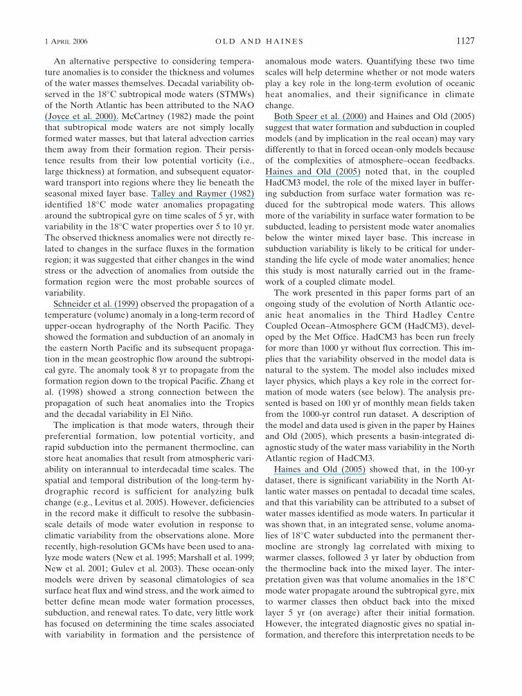
census of the waters in T–S space was made. Figure 1shows the census based on the 100 yr of data, with thevolume in each T–S bin defined as a percentage of thetotal volume. The water volumes have been sorted into0.5°C by 0.1 psu T–S bins. A significant feature of theT–S volume census for HadCM3, seen in Fig. 1, is thediagonal banding. This is a consequence of the discretelayering in the model, where the banding highlights thelow vertical resolution in the deeper model cells. Thedeep cold waters make up the largest percentage of thetotal volume; however there are three distinct modesformed in the warmer classes: a weak mode at 18.5°C,36.5 psu; a stronger mode at 16.5°C, 36.3 psu; and astrong mode at 14.0°C, 36.1 psu. These three modes arecomparable to the modes observed in the North Atlan-tic. In the analysis that follows the three mode waterswill be identified by their central temperatures; theseare 18.5° (STMW), 16.5° (MMW), and 14.0°C (SPMW).

The four key fields contributing to the formation ofmode waters (winter mixed layer depth, surface heatflux, P � E, and wind stress curl) have been calculatedfrom the 100 yr of HadCM3 data and are presented inFig. 2. The winter mixed layer base varies both spatiallyand interannually; for the analysis presented, the 100-yrlocal maximum mixed layer depth (Fig. 2a) has beenused to define the winter mixed layer base (WMLB).The equatorward shoaling of the mixed layer is clearlydefined and extends across the central North Atlantic;this corresponds to the New at al. (1995) subductionzone. There is an eastward increase in WMLB depth tothe north of the subduction zone, which extends intothe eastern North Atlantic. The general spatial struc-ture and depth of the HadCM3 winter mixed layer basecompare well with the recent mixed layer depth clima-tology produced by Kara et al. (2003). The climatologyshows the same deep trough extending across the basinbetween 30° and 50°N, with depths varying from 250 min the west to over 400 m in the east. The deep mixedlayer extends into the subpolar region and the Labra-dor Sea. Over the subtropical gyre, the climatologyshows the mixed layer to be shallower than 150 m, asdoes HadCM3, with the trough formed at 30°N on theeastern side of the basin beneath the trade winds. Themixed layer near the equator is shallower than 50 m inboth the climatology and HadCM3.

Figure 2b shows the 100-yr mean surface heat fluxinto the ocean. There is a region of strong heat loss overthe Gulf Stream and its extension at the western end ofthe deep WMLB trough. The depth of the WMLB inthis region is directly related to the significant heat lossincreasing the density and decreasing buoyancy. Equa-torward of the subduction zone, on average there isheating of the sea surface. This will tend to increase

1 APRIL 2006 O L D A N D H A I N E S 1129

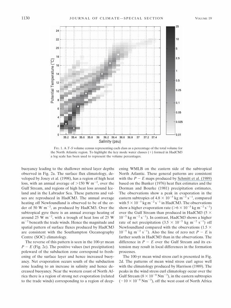
buoyancy leading to the shallower mixed layer depthsobserved in Fig. 2a. The surface flux climatology, de-veloped by Josey et al. (1998), has a region of high heatloss, with an annual average of �150 W m�2, over theGulf Stream, and regions of high heat loss around Ice-land and in the Labrador Sea. These patterns and val-ues are reproduced in HadCM3. The annual averageheating off Newfoundland is observed to be of the or-der of 50 W m�2, as produced by HadCM3. Over thesubtropical gyre there is an annual average heating ofaround 25 W m�2, with a trough of heat loss of 25 Wm�2 beneath the trade winds. Hence the magnitude andspatial pattern of surface fluxes produced by HadCM3are consistent with the Southampton OceanographyCentre (SOC) climatology.

The reverse of this pattern is seen in the 100-yr meanP � E (Fig. 2c). The positive values (net precipitation)poleward of the subduction zone correspond to fresh-ening of the surface layer and hence increased buoy-ancy. Net evaporation occurs south of the subductionzone leading to an increase in salinity and hence de-creased buoyancy. Near the western coast of North Af-rica there is a region of strong net evaporation (relatedto the trade winds) corresponding to a region of deep-

ening WMLB on the eastern side of the subtropicalNorth Atlantic. These general patterns are consistentwith the P � E maps produced by Schmitt et al. (1989)based on the Bunker (1976) heat flux estimates and theDorman and Bourke (1981) precipitation estimates.The observations show a peak in evaporation in theeastern subtropics of 4.8 � 10�5 kg m�2 s�1, comparedwith 5 � 10�5 kg m�2 s�1 in HadCM3. The observationsshow a higher evaporation rate (�6 � 10�5 kg m�2 s�1)over the Gulf Stream than produced in HadCM3 (5 �10�5 kg m�2 s�1). In contrast, HadCM3 shows a higherrate of net precipitation (3.5 � 10�5 kg m�2 s�1) offNewfoundland compared with the observations (1.5 �10�5 kg m�2 s�1). Also the line of zero net P � E isfarther south in HadCM3 than in the observations. Thedifference in P � E over the Gulf Stream and its ex-tension may result in local differences in the formationprocesses.

The 100-yr mean wind stress curl is presented in Fig.2d. The patterns of mean wind stress curl agree wellwith the climatology produced by Harrison (1989). Thepeaks in the wind stress curl climatology occur over theGulf Stream (8 � 10�8 Nm�3), in the eastern subtropics(�10 � 10�8 Nm�3), off the west coast of North Africa

FIG. 1. A T–S volume census representing each class as a percentage of the total volume forthe North Atlantic region. To highlight the key mode water classes (�) formed in HadCM3a log scale has been used to represent the volume percentages.

1130 J O U R N A L O F C L I M A T E — S P E C I A L S E C T I O N VOLUME 19

(8 � 10�8 Nm�3), and around Greenland (20 � 10�8

Nm�3). The magnitudes produced by HadCM3 com-pare well with the climatology. The lines of zero windstress curl define the separation between regions ofpoleward and equatorward Sverdrup interior flow. Thenorthern line of zero wind stress curl slopes to thenortheast across the basin. All points along this line arepoleward of the shoaling of the WMLB. The meridi-onal gradient in the wind stress curl on the western sideof the basin is steep, suggesting that there is little spatialmovement in the zero line. The meridional gradient isweak on the eastern side of the basin, indicating thatthe zero line may show greater variability in latitude,

which will affect both the formation and equatorwardpropagation of the volume anomalies formed on theeastern side of the basin. The line of zero wind stresscurl that bounds the equatorward side of the subtropi-cal gyre region shows the reverse pattern of meridionalgradient, with steep gradients in the east and shallowgradients in the west.

Marshall et al. (1993) estimated the annual kinematicsubduction rate using the equation

Sann � �uH � �H � wH. �1�

The overbar denotes annual means, H is the depth ofthe winter mixed layer base (defined by the fixed

FIG. 2. (a) The 100-yr max WMLB depth (m). The light shading highlights depths �300 m, and the darkershading depths �500 m. (b) The 100-yr mean surface heat flux for the North Atlantic Region of HadCM3 (W m�2).The shaded region highlights negative values. (c) The 100-yr mean P � E (�10�5 kg m�2 s�1). (Negative valuesare shaded.) (d) The 100-yr mean wind stress curl (�10�8 N m�3). (Negative values are shaded.)

1 APRIL 2006 O L D A N D H A I N E S 1131

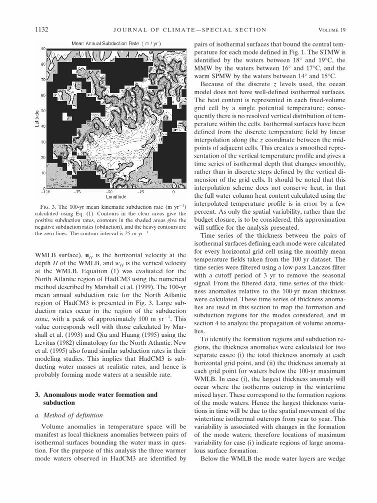
WMLB surface), uH is the horizontal velocity at thedepth H of the WMLB, and wH is the vertical velocityat the WMLB. Equation (1) was evaluated for theNorth Atlantic region of HadCM3 using the numericalmethod described by Marshall et al. (1999). The 100-yrmean annual subduction rate for the North Atlanticregion of HadCM3 is presented in Fig. 3. Large sub-duction rates occur in the region of the subductionzone, with a peak of approximately 100 m yr�1. Thisvalue corresponds well with those calculated by Mar-shall et al. (1993) and Qiu and Huang (1995) using theLevitus (1982) climatology for the North Atlantic. Newet al. (1995) also found similar subduction rates in theirmodeling studies. This implies that HadCM3 is sub-ducting water masses at realistic rates, and hence isprobably forming mode waters at a sensible rate.

3. Anomalous mode water formation andsubduction

a. Method of definition

Volume anomalies in temperature space will bemanifest as local thickness anomalies between pairs ofisothermal surfaces bounding the water mass in ques-tion. For the purpose of this analysis the three warmermode waters observed in HadCM3 are identified by

pairs of isothermal surfaces that bound the central tem-perature for each mode defined in Fig. 1. The STMW isidentified by the waters between 18° and 19°C, theMMW by the waters between 16° and 17°C, and thewarm SPMW by the waters between 14° and 15°C.

Because of the discrete z levels used, the oceanmodel does not have well-defined isothermal surfaces.The heat content is represented in each fixed-volumegrid cell by a single potential temperature; conse-quently there is no resolved vertical distribution of tem-perature within the cells. Isothermal surfaces have beendefined from the discrete temperature field by linearinterpolation along the z coordinate between the mid-points of adjacent cells. This creates a smoothed repre-sentation of the vertical temperature profile and gives atime series of isothermal depth that changes smoothly,rather than in discrete steps defined by the vertical di-mension of the grid cells. It should be noted that thisinterpolation scheme does not conserve heat, in thatthe full water column heat content calculated using theinterpolated temperature profile is in error by a fewpercent. As only the spatial variability, rather than thebudget closure, is to be considered, this approximationwill suffice for the analysis presented.

Time series of the thickness between the pairs ofisothermal surfaces defining each mode were calculatedfor every horizontal grid cell using the monthly meantemperature fields taken from the 100-yr dataset. Thetime series were filtered using a low-pass Lanczos filterwith a cutoff period of 3 yr to remove the seasonalsignal. From the filtered data, time series of the thick-ness anomalies relative to the 100-yr mean thicknesswere calculated. These time series of thickness anoma-lies are used in this section to map the formation andsubduction regions for the modes considered, and insection 4 to analyze the propagation of volume anoma-lies.

To identify the formation regions and subduction re-gions, the thickness anomalies were calculated for twoseparate cases: (i) the total thickness anomaly at eachhorizontal grid point, and (ii) the thickness anomaly ateach grid point for waters below the 100-yr maximumWMLB. In case (i), the largest thickness anomaly willoccur where the isotherms outcrop in the wintertimemixed layer. These correspond to the formation regionsof the mode waters. Hence the largest thickness varia-tions in time will be due to the spatial movement of thewintertime isothermal outcrops from year to year. Thisvariability is associated with changes in the formationof the mode waters; therefore locations of maximumvariability for case (i) indicate regions of large anoma-lous surface formation.

Below the WMLB the mode water layers are wedge

FIG. 3. The 100-yr mean kinematic subduction rate (m yr�1)calculated using Eq. (1). Contours in the clear areas give thepositive subduction rates, contours in the shaded areas give thenegative subduction rates (obduction), and the heavy contours arethe zero lines. The contour interval is 25 m yr�1.

1132 J O U R N A L O F C L I M A T E — S P E C I A L S E C T I O N VOLUME 19

shaped, with the thin end of the wedge being equator-ward of the subduction region. This thinning is a con-sequence of the conservation of potential vorticity(PV), where

PV �f � �

h. �2�

Mode waters are formed with a low PV and away fromthe western boundary current f �. Therefore, as themode waters are advected equatorward away fromtheir formation regions, the planetary vorticity f de-creases; therefore the thickness of the layer h must de-crease to conserve PV. Hence for case (ii) the largestthickness occurs where the isotherms intersect with theWMLB. This corresponds to the regions where subduc-tion or obduction of water volume will occur. These arealso the locations where the largest variability will oc-cur; therefore locations of maximum variability for case(ii) indicate the regions of large anomalous mode watersubduction.

b. Mode water formation regions

Spatial maps of the standard deviation in total thick-ness anomalies used to identify the formation regionsfor the three modes are shown in Figs. 4a,c,e. All threemodes have broad regions of large variability showingthe extent of the formation regions. The STMW (18°–19°C) spans 27.5° to 37.5°N and 70° to 45°W (Fig. 4a),the MMW (16°–17°C) spans 30° to 41°N and 60° to25°W (Fig. 4c), and the warm SPMW spans 35° to 45°Nand 50° to 10°W (Fig. 4e). The large spatial extent ofthe formation regions is due to two possible processes.1) The horizontal movement of the seasonal mixedlayer isothermal structure, which is equivalent tochanges in the wintertime sea surface temperature pat-tern. 2) The interannual changes in the depth of thewinter mixed layer base, which is related to the strengthof the wintertime deep convection. In practice both ofthese processes are likely to occur simultaneously.

All three modes show a double peak in their forma-tion region, suggesting a bimodal state during this 100-yr period. The formation regions for the three modestogether span the west–east extent of the North Atlan-tic subduction zone, and there is minimal overlap be-tween the three formation regions. This shows a shift inmode water temperature to cooler classes from west toeast across the basin. The magnitude of the peak thick-ness anomaly increases from 70 m in the west (STMW)to 100 m in the east (SPMW). However, we do not seea continuous range of modes between the STMW andSPMW (see Fig. 1), indicating that there are processes

that inhibit the formation of waters in the intermediatetemperature ranges.

c. Mode water subduction regions

Spatial maps of the standard deviation in the thick-ness anomalies below the WMLB used to identify thesubduction regions for the three modes are shown inFigs. 4b,d,f. The STMW (18°–19°C) subduction region(Fig. 4b) forms a narrower band than the formationregion while retaining the corresponding double peakstructure. There is a weak peak at 28°N, 56°W and astrong peak at 30°N, 49°W. A meridional section ofpotential temperature taken at 50°W (Fig. 5a) forMarch (i.e., the end of winter) of year 3 of the datasetshows that 30°N corresponds to the intersection of the18° and 19°C isothermal surfaces with the WMLB, sug-gesting that this is the latitude of subduction for theSTMW.

The subduction region for the MMW (16°–17°C; Fig.4d) is broader than that of the STMW and shows twovery distinct peaks at 33°N, 39°W and 34°N, 26°W. Ameridional section of potential temperature taken at30°W (Fig. 5b) for March of year 3 shows that 34°Ncorresponds to the intersection of the 16° and 17°Cisothermal surfaces with the WMLB, suggesting thatthis is the latitude of subduction for the MMW.

The main subduction region for the warm SPMW(14°–15°C), shown in Fig. 4f, is very close to the easternboundary of the basin and in the region of deepeningWMLB (see Fig. 2a). There is a weak double peakstructure in the warm SPMW subduction, with a strongpeak at 36°N, 21°W and a weak peak at 39°N, 18°W.Figure 5c shows the meridional section of potentialtemperature taken at 20°W for March of year 3, high-lighting the relationship between the isothermal surfaceand the strong subduction peak at 36°N, 21°W.

d. Variability in mode water subduction

Time series of unfiltered thickness anomalies belowthe WMLB at the main subduction locations (Fig. 5) foreach mode are presented in Fig. 6. The two variabilitymaxima observed for each mode will be identified asthe western peak (Fig. 6a) and the eastern peak (Fig.6b).

The SPMW (14°–15°C) layer thickness (thick dashedlines) shows large variability at both the western andeastern locations during the first 50 yr of the dataset,with some anticorrelation between them. Over the sec-ond 50 yr, there is very little thickness variability in theeast. The thickness at the western location variesstrongly over time scales of 5 to 20 yr, with the largestvariations occurring on the longer time scales. The

1 APRIL 2006 O L D A N D H A I N E S 1133

1134 J O U R N A L O F C L I M A T E — S P E C I A L S E C T I O N VOLUME 19

MMW (16°–17°C) thickness (thin solid lines) showslarge variability at both the western and eastern loca-tions throughout the 100-yr period, and the two timeseries also show some anticorrelation. There are peri-ods when the thickness below the WMLB goes to zero

at the eastern location. This is due either to the move-ment of the isothermal outcrop southward, away fromthis location, or the vertical movement of the layer sothat it intersects the fixed WMLB farther south. TheSTMW (18°–19°C) thick solid lines show strong vari-

FIG. 5. Three meridional sections taken from March of year 3 in the dataset showing the latewinter (Northern Hemisphere) potential temperature structure in the North Atlantic Ocean.(a) Meridional section at 50°W highlighting the 18°–19°C STMW. (b) Meridional section at30°W highlighting the 16°–17°C MMW. (c) Meridional section at 20°W highlighting the14°–15°C SPMW. The dashed lines define the upper and lower bounds of the seasonal mixedlayer.

←

FIG. 4. Maps of std dev in the thickness anomaly (m) between pairs of isothermal surface in the total water column (formation) andbelow the WMLB (subduction) for the three classes considered. (a) Formation and (b) subduction regions for the 18°–19°C water class.(c) Formation and (d) subduction regions for the 16°–17°C water class. (e) Formation and (f) subduction regions for the 14°–15°C waterclass. The heavy line shows the furthest extent of the isothermal outcrop. The contour interval is 10 m, and the location of the formationand subduction peaks for each class is indicated.

1 APRIL 2006 O L D A N D H A I N E S 1135

ability throughout the 100-yr period, with larger vari-ability at the eastern location. The western locationshows some 20-yr periodicity, whereas at the easternlocation there are a series of separate strong events thateach last approximately 5 yr. The thickness of theSTMW in the eastern location periodically goes to zeroas the isothermal outcrop of this mode moves equator-ward from this location.

Comparing the thickness variability between the dif-ferent modes for the western locations, Fig. 6a showsthat, over the first 40 yr of the dataset, the events in themodes appear to be lagged in time starting with theSTMW on the western side of the basin and ending withthe SPMW on the eastern side of the basin. The lagbetween the STMW and SPMW events are of the order

of 8 yr. At present it is not clear what causes this lag.The most probable candidates are the propagation of avolume anomaly along the North Atlantic Current, agradual meridional shift in the wind field, and changesin the surface heat fluxes. The complex interaction be-tween these three processes makes it difficult to iden-tify a leading cause. During the second half of the 100-yr dataset, there appears to be little correlation be-tween the modes.

Thickness variability events for the eastern locations(Fig. 6b) for all modes are generally larger than those atthe western locations. Between years 15 and 30 thereare coherent events of the same sign in all three modes,suggesting a basinwide change in the forcing. After 40yr the SPMW (14°–15°C) shows very little variability,

FIG. 6. Unfiltered time series of layer thickness (m) below the WMLB for the three modewater classes taken from (a) the western and (b) the eastern peaks shown in Fig. 4. Thewestern peak locations are as follows: STMW (28°N, 56°W), MMW (33°N, 39°W), and warmSTMW (36°N, 21°W). The eastern peak locations are as follows: SPMW (30°N, 49°W), MMW(34°N, 26°W), and warm SPMW (39°N, 18°W).

1136 J O U R N A L O F C L I M A T E — S P E C I A L S E C T I O N VOLUME 19

indicating that the main subduction variability occurs atthe western location. However, for both the STMW andMMW there are periodic large events in the easternsubduction locations.

These data indicate that formation and subductionvariations occur on periods of 5 to 20 yr. The dualsubduction locations appear to result from a change inthe gyre dynamics and/or a shift in the wind field lead-ing to a northeast shift in the main subduction regionsfor all modes. Changes in the SPMW formed on theeastern side of the basin tend to lag changes in theSTMW formed on the western side by around 8 yr, asseen in Fig. 6a by the offset in peaks between locations.The northeast shift in the subduction region produceslarger subduction events at the eastern variability peakfor each mode water class. As a consequence theseevents are likely to produce the strongest coherent sig-nals for propagating anomalies, and will therefore beused in the following section to study the persistence ofvolume anomalies.

4. Persistence and propagation of subductedanomalies

a. Mapping propagating thickness anomalies

In section 3 it was shown that the regions of largestthickness variability, and hence large anomalous sub-duction, are localized. To show that the subducted vol-ume anomalies persist and propagate beneath theWMLB, the thickness anomalies at the peak subduc-tion locations (Fig. 4) for each mode were lag corre-lated against the thickness anomalies at all other loca-tions. For example, Fig. 7a(i) shows the maximumthickness correlation detected for any lag time. A mapof the lag times for the maximum correlation, at alllocations where Fig. 7a(i) is statistically significant,shows the spatial propagation of the volume anomaly[e.g., Fig. 7a(ii)]. Lagged regressions of the standard-ized thickness anomalies are used to define the percent-age of the remote thickness variability explained by theanomalous subduction [e.g., Fig. 7a(iii)].

By lag correlating the thickness anomalies at thepeak subduction locations for each mode against thethickness anomalies in adjacent water mass classes(e.g., Figs. 7b,c), it is also possible to show that thevolume anomalies are transformed into adjacent classesfrom the original water mass class as the anomalypropagates. This is equivalent to determining the wayin which the heat associated with the anomaly diffusesas the anomaly propagates around the system. In gen-eral if the anomaly transforms to warmer classes, thenit moves up through the water column, conversely if the

anomaly transforms to colder classes then it movesdownward through the water column.

In the following, the results for each mode will bepresented separately. For each mode a set of mapsshowing (i) the maximum correlation coefficients, (ii)lag times, and (iii) percentage of remote variability ex-plained is presented. Lagged correlations against thewater mass defining the mode, and against thermallyadjacent water masses, are shown.

b. Subtropical mode waters (18°–19°C)

The lagged correlations for the two STMW subduc-tion locations show similar patterns, with those of theeastern location (30°N, 49°W) giving stronger signals;therefore only these results are presented. Figure 7shows the maximum correlation of STMW (18°–19°C)thickness anomalies below the WMLB at 30°N, 49°Wagainst thickness anomalies in 18°–19°C waters (Fig.7a), thickness anomalies in 19°–20°C waters (Fig. 7b),and thickness anomalies in 20°–21°C waters (Fig. 7c).

The statistically significant correlations for thicknessanomalies in the same class (18°–19°C) of waters areeverywhere positive [Fig. 7a(i)]. The lag times [Fig.7a(ii)] are nearly all positive, that is, variability lagsvariability at the peak subduction location, which isconsistent with the advection of anomalies away fromthe subduction region equatorward and westwardaround the gyre. The time scale for the propagation ison the order of 5 yr. The regression map in [Fig. 7a(iii)]shows that over the majority of the region of statisticalsignificance more than 60% of the remote variabilitycan be explained by the variability in the subductionregion, with the percentage explained decreasing withdistance from the source.

The adjacent warmer classes also both show regionsof statistically significant positive correlation. The lagtimes for the 19°–20°C waters [Fig. 7b(ii)] show that theearliest impact on this water layer lags the STMW sub-duction anomaly at (30°N, 49°W) by approximately 1yr. The lag times extend out to 5 yr, moving south andwest, and 50%–75% of the remote variability is typi-cally explained by the anomalous subduction of STMW[Fig. 7b(iii)]. There is a small region of positively cor-related thickness anomalies in the 20°–21°C waters[Fig. 7c(i)] at the southwest extreme of the 18°–19°Cpropagation region. The earliest impact on this waterclass lags the STMW subduction anomaly by approxi-mately 2 yr [Fig. 7c(ii)], and the subduction generallyaccounts for less than 60% of the remote variability[Fig. 7c(iii)]. These results are consistent with the trans-formation of STMW volume anomalies upward towardwarmer classes as a mechanism for mode water decaywithin the thermocline.

1 APRIL 2006 O L D A N D H A I N E S 1137

The transformation of STMW to warmer classes isconsistent with the transformation path that was foundto dominate in the basin-integrated diagnostics derivedby Haines and Old (2005). Using the integrated diag-nostic it was possible to quantify the mixing processesresponsible for the transformations. Here it is possibleto see in detail the spatial distributions, range of lag

times, and the percentage of variance explained, andhence the predictable variance in the different locations.

Lag correlations of STMW subduction anomaliesagainst thickness anomalies in the colder classes 17°–18°C, 16°–17°C, and 15°–16°C are presented in Figs.8a,b,c, respectively. For the 17°–18°C water mass (Fig.8a), immediately beneath the STMW there is a dipole

FIG. 7. Spatial maps of (i) max lag correlation, (ii) lag time at max for statistically significant correlations, and (iii) the percentage ofremote variability explained in thickness anomalies below the WMLB relative to the point (x) of max 18°–19°C subduction variabilityat 30°N, 49°W, as defined in Fig. 4b. Correlated thickness variability of (a) 18°–19°C waters, (b) 19°–20°C waters, and (c) 20°–21°Cwaters against variability in 18°–19°C subduction thickness. All data were low-pass filtered using a Lanczos filter with a 3-yr cutoffperiod.

1138 J O U R N A L O F C L I M A T E — S P E C I A L S E C T I O N VOLUME 19

Fig 7 live 4/C

pattern of correlation [Fig. 8a(i)]. To the west of thesubduction region the anomalies are negatively corre-lated, while to the east they are positively correlated.The lag times [Fig. 8a(ii)] again suggest the propagationof anomalies southward around the gyre away from thesubduction region, and for both regions the lag timesare up to 5 yr. For the western negative correlationregion, up to 80% of the remote variance is explainedby the subduction anomalies, while in the eastern

positive correlation region, less than 60% is explained[Fig. 8a(iii)].

The positively correlated region to the east cannot bedue to propagation from the subduction region as thereis a zero lag for the earliest impact; this suggests thatthis correlation results from the correlated formation ofwaters in the 17°–18°C water mass. This is consistentwith the observed decrease in dominant mode watertemperature moving eastward across the basin. The an-

FIG. 8. Same as in Fig. 7, but at 30°N, 49°W. Correlated thickness variability of (a) 17°–18°C waters, (b) 16°–17°C waters, and (c)15°–16°C waters against variability in 18°–19°C subduction thickness.

1 APRIL 2006 O L D A N D H A I N E S 1139

Fig 8 live 4/C

ticorrelated region to the west suggests that the vari-ability here results from the anomalous formation ofthe 18°–19°C waters at the expense of 17°–18°C watersthrough a shift in the formation/subduction regions.This interpretation is also consistent with the extent ofthe high thickness variability for the 18°–19°C modewaters in Fig. 4a, which extends westward from thepeak at 30°N, 49°W.

The two colder classes (16°–17°C and 15°–16°C)show similar patterns of anticorrelation [Figs. 8b(i) and8c(i)], with lag times out to 5 yr [Figs. 8b(ii) and 8c(ii)].For the 16°–17°C class, up to 80% of the remote vari-ability is explained by the anomalous subduction [Fig.8b(iii)], while up to 70% is explained for the 15°–16°Cwaters [Fig. 8c(iii)]. This pattern of anticorrelation isrepeated down to 13°C waters, below which there is nosignificant correlation (data not presented). This sug-gests that subduction of a positive anomaly of 18°–19°Cwater is associated with a loss of waters in the lowerthermocline classes beneath the subduction region.

If the thickness of the 18°–19°C water class below thefixed WMLB is increased, then the thickness of someother temperature layers must decrease at the sametime to make room for the 18°–19°C water. However,the integrated transformation diagnostics in Haines andOld (2005) do not indicate any transformations be-tween the 15°–16°C and the 18°–19°C water classes.This implies that the reduction in thickness of thecolder waters is a dynamical effect, with divergence/convergence of the colder classes allowing for the pres-ence of the 18°–19°C mode water anomalies above.

c. Madeira Mode Waters (16°–17°C)

The Madeira Mode Waters (16°–17°C) also show twodistinct locations of maximum subduction variability.Lag correlation results for both peaks show differentresponses; therefore, the analysis for both locations willbe presented. The analysis for the western subductionlocation at 33°N, 39°W is shown in Fig. 9, and the analy-sis for the eastern location at 34°N, 26°W in Fig. 10.Spatial maps of the correlations of the MMW sub-duction anomalies against the 15°–16°C, 16°–17°C(MMW), and 17°–18°C thickness anomalies are pre-sented for the two subduction regions.

The main results for the western peak at 33°N, 39°Ware that the subducted anomalies propagate away fromthe subduction region around the subtropical gyre[Figs. 9b(i) and 9b(ii)] with significant correlations seenfor up to 8 yr. This is considerably longer than for theSTMW, which is perhaps consistent with the location ofthe MMW subduction, that is, farther from the centerof the gyre and in a region of lower flow. Unlike the

STMW, the MMW thickness anomalies are anticorre-lated with the anomalies in the layer immediately abovethem in the water column [17°–18°C; Fig. 9c(i)] andthese anticorrelated anomalies do not appear to propa-gate very far around the gyre. However, for the colderwater class (15°–16°C) there is a double branch in thecorrelation pattern, with both branches being positivelycorrelated with the subduction anomalies [Fig. 9a(i)].The lag times [Fig. 9a(ii)] in both branches extend outto 7 yr. Both branches start with zero lag in relation tothe subduction anomaly, suggesting that they resultfrom the correlated formation of waters in this colderclass. This correlated formation will mask any signal ofthe transformation of waters with adjacent classes. Thisobservation suggests that the anomalies are not re-moved via transformation into adjacent classes; an al-ternative mechanism for their removal will be discussedin section 5.

The eastern peak at 34°N, 26°W produces largeranomalies and longer lag times [of the order of 10 yr inFig. 10b(ii)]. The correlation of the subduction anoma-lies against the 16°–17°C waters [Fig. 10b(i)] shows adouble branch, with the western branch being anticor-related and the eastern branch positively correlated.The western branch coincides with the region of posi-tive correlation for the western subduction peak at33°N, 39°W seen in Fig. 9b(ii). This anticorrelation sug-gests that the dual subduction peaks result from a shifteastward in the isotherm structure. Figure 10a(i) showsthe thickness anomalies in the waters beneath theMMW to be anticorrelated with the anomalies in theMMW subduction region, that is, the colder classes aredisplaced by the subduction of positive volume anoma-lies. The anomalies in the waters immediately abovethe MMW [Fig. 10c(i)] are positively correlated withthe subducted anomalies. The shortest lag time is 0 yrimmediately adjacent to the subduction region and ex-tends out to 10 yr at the southern limit of the statisti-cally significant region. The anomalies in this layertravel faster than those in the MMW layer, suggestingthat the observed correlations are more likely to be dueto coformation rather than transformation betweenclasses.

d. Warm subpolar mode waters (14°–15°C)

For the warm SPMW class the western subductionpeak at 36°N, 21°W shows strong correlation signals,while the weaker eastern peak at 39°N, 18°W does not;therefore, only the results for the western peak areshown in Fig. 11. The figure includes maps of the cor-relation of the warm SPMW thickness anomalies at thesubduction location against the 13°–14°C (Fig. 11a),

1140 J O U R N A L O F C L I M A T E — S P E C I A L S E C T I O N VOLUME 19

14°–15°C (warm SPMW; Fig. 11b), and 15°–16°C (Fig.11c) thickness anomalies.

There is an extensive region of strong positive cor-relation [Fig. 11b(i)] associated with the thicknessanomalies in the subduction region. The lag times inFig. 11b(ii) show a broad area of essentially zero lagaround the subduction location, highlighting the wideextent of the subduction region. Once again lag times ofup to 10 yr imply the propagation of the anomaliesaway from the subduction region equatorward and

westward around the gyre. Over most of the region,more than 80% of the remote variability is explained bythe thickness anomalies in the subduction region [Fig.11b(iii)], that is, the subducted volume anomalies ofwarm SPMW produce propagating signals that are co-herent for more than 10 yr and hence should be pre-dictable. This strong coherence also means that heatanomalies produced by anomalous subduction in thisclass will persist for up to 10 yr.

The warmer water mass (15°–16°C) immediately

FIG. 9. Same as in Fig. 7, but for 16°–17°C subduction variability at 33°N, 39°W, as defined in Fig. 4d. Correlated thickness variability of(a) 15°–16°C waters, (b) 16°–17°C waters, and (c) 17°–18°C waters against variability in 16°–17°C subduction thickness.

1 APRIL 2006 O L D A N D H A I N E S 1141

Fig 9 live 4/C

above the warm SPMW has a region of negative cor-relation [Fig. 11c(i)] above the SPMW subduction re-gion. This can be interpreted as a shift in the isothermaloutcrops equatorward, leading to the formation ofcooler 14°–15°C waters at this location. Equatorward ofthe SPMW subduction region there is an extended re-gion of positive correlation. The lag times [Fig. 11c(ii)]and regression coefficients [Fig. 11c(iii)] indicate thatthis region of positive correlation in the warmer class isdue to correlated formation. This is also consistent withthe equatorward movement of the isotherms leading to

a change in position of the formation regions for watersmasses that are adjacent in temperature class. Figure 5calso supports this interpretation, as it shows that theshoaling region of the WMLB has a shallower slopenear the eastern side of the basin. There are thick layersof both 14°–15°C and 15°–16°C waters beneath theWMLB along this meridional section at 20°W. The cor-relations with the 16°–17°C waters (data not shown) arenegative, indicating the displacement of these warmerwaters by the SPMW classes below.

In contrast, the thickness anomalies in the colder

FIG. 10. Same as in Fig. 9, but at 34°N, 26°W.

1142 J O U R N A L O F C L I M A T E — S P E C I A L S E C T I O N VOLUME 19

Fig 10 live 4/C

class of waters (13°–14°C), shown in Fig. 11a, are posi-tively correlated with the subducted thickness anoma-lies of the warm SPMW (14°–15°C). Again the lag timesand regression coefficients suggest that this correlationis the result of correlated formation. It is interesting tonote that the propagation of the signal in this colderclass is interrupted around 25°N. This corresponds tothe region of deepening WMLB (as seen in Fig. 2a) dueto the increased evaporation by the trade winds. Figure5a also shows that there is a strong 18°–19°C ther-

mocline formed in this region that tends to pinch off thecolder classes below. These features suggest that this isan obduction region (consistent with Fig. 3), where thelateral advection is carrying waters back into the sea-sonal mixed layer across the WMLB.

5. Discussion

It has been shown that persistent volume anomaliesform in the warm mode waters of the North AtlanticOcean in the HadCM3 climate model. Analysis of the

FIG. 11. Same as in Fig. 7, but for 14°–15°C subduction variability at 36°N, 21°W, as defined in Fig. 4f. Correlated thickness variability of(a) 13°–14°C waters, (b) 14°–15°C waters, and (c) 15°–16°C waters against variability in 14°–15°C subduction thickness.

1 APRIL 2006 O L D A N D H A I N E S 1143

Fig 11 live 4/C

100 yr of data taken from the control run has shownthat the time scales associated with the variability information of North Atlantic mode water ranges from 5to 20 yr. For some events there was a west–east lag of8 yr in the anomalous formation across the basin. Thisis consistent with the observed time scale for the propa-gation of heat anomalies in the upper ocean along theNorth Atlantic Current (Hansen and Bezdek 1996; Sut-ton and Allen 1997), suggesting that this is one possiblecause for the lagged anomalous formation across thebasin.

The key process leading to the persistence of theseanomalies is their subduction beneath the winter mixedlayer base where they are effectively isolated from thesurface forcing. Once beneath the WMLB, the volumeanomalies propagate equatorward away from the sub-duction region and move as part of the general gyrecirculation. The persistence time of volume anomaliesincreases with distance east of the center of the sub-tropical gyre. This is consistent with the increase insubduction depth and decrease in circulation with dis-tance east of the subtropical gyre center. The STMWanomalies formed on the western side of the basin typi-cally persist for up to 5 yr after they are subductedbeneath the winter mixed layer base. Moving eastward,MMWs are formed over a region spanning from 40°Wabove the mid-Atlantic ridge to 20°W. The subductedMMW anomalies persist for up to 8–10 yr as they travelaround the gyre in the general circulation. On the east-ern side of the basin the SPMW anomalies subductedbeneath the WMLB persist for up to 10 yr as theypropagate around the gyre.

For all three modes it was shown that anomalousvolumes are on average formed at the expense of thecolder temperature classes; therefore, the formation ofa positive volume anomaly results in warming, or oceanheat storage. Because of the shorter propagation times,and hence shorter persistence, nearer the gyre center,the STMW will only contribute to ocean heat anomalieson time scales of up to 5 yr. The persistence times of upto 10 yr for the modes formed on the eastern side of thebasin, implies that they play an important role in thedecadal storage of ocean heat anomalies. The persis-tence of volume (heat) anomalies is equivalent to theocean’s memory of warming or cooling climatic events.

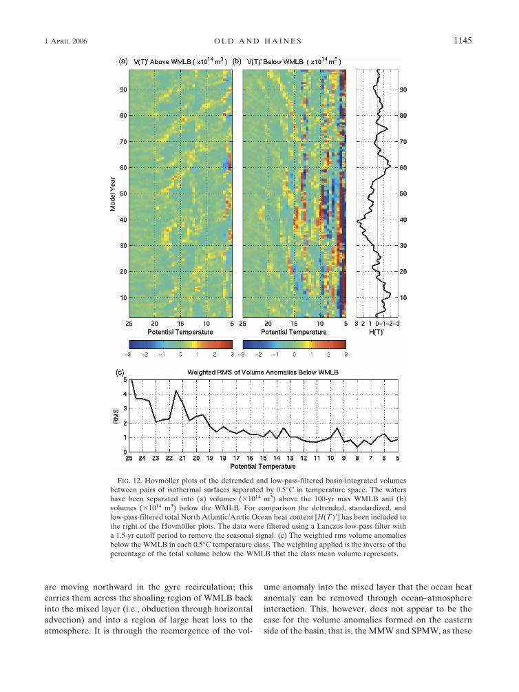
The persistence times of volume anomalies in par-ticular temperature ranges can be seen in a time seriesof the basin-integrated volumes based on the potentialtemperature. Figure 12 presents Hovmöller plots of thebasin-integrated volumes between pairs of isothermalsurface that are 0.5°C apart in temperature space. Thedata have been detrended and low-pass filtered, using a

Lanczos filter with a cutoff period of 1.5 yr, to removethe seasonal cycle.

Figure 12a presents a Hovmöller plot of the timevariation in the total volumes of water above theWMLB, sorted into 0.5°C temperature bands. This fig-ure shows the formation of volume anomalies around18°C and the subsequent propagation to colder classesin time. As these volumes are above the WMLB, thisprocess occurs completely within the seasonal mixedlayer. As these upper-ocean heat anomalies propagateacross the North Atlantic basin along the Gulf Streamextension/NAC, they lose heat to the atmosphere andare transformed to colder water classes. For example, alarge volume anomaly forms in the mixed layer be-tween 17° and 18°C around year 32 and subsequentlypropagates to colder classes over the following 8 yr.

Figure 12b shows the volumes below the WMLB fortemperature classes in the range of 5° to 25°C. To theright of the figure is a plot of the detrended, standard-ized, and low-pass-filtered (Lanczos, 1.5-yr cutoff) totalheat content anomaly for the 100 yr. This figure showsthat large volume changes occur in the classes aroundthe main North Atlantic Mode Waters and below theWMLB. Around 40 yr into the time series there is alarge positive heat anomaly in the North Atlantic basin.This is distributed amongst the main mode temperatureclasses seen in Fig. 1, of 7°, 10°, 14° and 16°C. Figure12b highlights the role that mode waters, particularlythose formed on the eastern side of the basin, play inthe long-term ocean heat storage.

To further determine whether particular classes havegreater variability than others, the rms of the anomaliesin time for each temperature class was calculated. Ingeneral there is an increase in the magnitude of theanomalies going from warmer to colder classes. This isa consequence of the increasing contribution to the to-tal volume of each class going from warm to coldclasses. To minimize this volume effect in the rms of theanomalies, the rms values were weighted according tothe percentage their temperature class contributed tothe total basin volume. The weighted rms values, pre-sented in Fig. 12c, show distinct peaks associated withthe main mode waters, in particular 14°–15°C, 16°–17°C, and 18°C. It also highlights the colder subpolarmodes at 13°–14°C, 9°–10°C, and 6°C.

In the absence of any long-term changes in the totalheat content, any volume anomalies formed in a par-ticular temperature range must be removed. For theSTMW it was shown that there is transformation of the18°–19°C waters to warmer classes as the volumeanomaly propagates around the gyre. At the westernextent of the propagation region the volume anomalies

1144 J O U R N A L O F C L I M A T E — S P E C I A L S E C T I O N VOLUME 19

are moving northward in the gyre recirculation; thiscarries them across the shoaling region of WMLB backinto the mixed layer (i.e., obduction through horizontaladvection) and into a region of large heat loss to theatmosphere. It is through the reemergence of the vol-

ume anomaly into the mixed layer that the ocean heatanomaly can be removed through ocean–atmosphereinteraction. This, however, does not appear to be thecase for the volume anomalies formed on the easternside of the basin, that is, the MMW and SPMW, as these

FIG. 12. Hovmöller plots of the detrended and low-pass-filtered basin-integrated volumesbetween pairs of isothermal surfaces separated by 0.5°C in temperature space. The watershave been separated into (a) volumes (�1014 m3) above the 100-yr max WMLB and (b)volumes (�1014 m3) below the WMLB. For comparison the detrended, standardized, andlow-pass-filtered total North Atlantic/Arctic Ocean heat content [H(T )] has been included tothe right of the Hovmöller plots. The data were filtered using a Lanczos low-pass filter witha 1.5-yr cutoff period to remove the seasonal signal. (c) The weighted rms volume anomaliesbelow the WMLB in each 0.5°C temperature class. The weighting applied is the inverse of thepercentage of the total volume below the WMLB that the class mean volume represents.

1 APRIL 2006 O L D A N D H A I N E S 1145

Fig 12 live 4/C

anomalies do not propagate far enough around the gyreand are too deep to be obducted back into the mixedlayer.

For all three modes there are no coherent signalsassociated with the subducted thickness anomaliessouth of 20°N. There is a region of net heat loss fromthe ocean to the atmosphere south of 20°N (Fig. 2b)that lies beneath the trade winds. The trade winds formthe boundary of the tropical–subtropical water massexchange region discussed by Liu et al. (1994). Theypropose that tropical–subtropical water mass exchangeis a consequence of the shallow (300 m) overturning cellextending from the equator into the subtropics, drivenby the Ekman transport of the easterly trade winds.This cell interacts with the equatorial cell that drivesthe countercurrent. The pathway taken by a water par-cel depends on the depth at which it reaches the Ekmancell. Figure 5b shows that the MMWs are blocked bythe equatorial countercurrent (centered at 10°N) thatbrings colder waters up from the western boundary tothe surface. Therefore, MMW anomalies will probablyrejoin the system at the western boundary near the startof the Gulf Stream. Figure 5c indicates that the SPMWfeeds directly into the countercurrent region. ThereforeSPMW anomalies may return to the surface via theequatorial countercurrent or by upwelling at the equa-tor as part of the Ekman overturning cell.

The analysis of the HadCM3 data indicates that theanomalies formed in the MMW and SPMW are notsignificantly transformed to the surrounding classes asthey propagate around the subtropical gyre. The tropi-cal–subtropical exchange region seems to be the mostprobable region where the heat anomalies stored in thedeeper modes will reemerge to release their heat to theatmosphere. It should be noted that Harper (2000)showed, using tracer experiments, that this process iscomplicated by the basin topography in the North At-lantic, and that it is possible that waters entrained intothis cell from the subtropics actually reemerge in theGulf of Mexico. More work is required to fully under-stand the reemergence of the deeper heat anomaliesand their impact on climate variability.

The long coherence time of the propagating volumeanomalies observed near the eastern side of the basinimplies the presence of signals in the ocean hydrogra-phy that may give predictability out to 10 yr. It shouldbe noted that these results are based on observationsfrom a fairly low resolution model. The ocean compo-nent of the model is not eddy permitting and will there-fore not contain the high-frequency natural variabilitythat exists in the real world. This may affect the mixingrates in the formation regions and will lead to a morestable Gulf Stream extension, that is, it will preclude

meanders. The absence of these processes means thatthe model signals are possibly too smooth, contributingto the spatially coherent high correlation and regressionvalues observed in the analysis. In reality it may bemore difficult to find these signals in the observationalrecord. However, the model observations provide goodphysical grounds for seeking persistent signals in thispart of the North Atlantic. The potential for volumeanomalies to enter the Tropics through tropical–subtropical water mass exchange processes beneath thetrade winds suggests the possibility of a strong atmo-spheric feedback, and the time scales involved suggest apotential climate feedback.

On much longer time scales, changes in the meridi-onal overturning circulation (MOC) are likely to drivelarge-scale climate changes through ocean basin ex-changes. Density-driven processes (e.g., deep convec-tive mixing/overturning) in the high latitudes of the At-lantic Ocean and the Arctic Ocean will influence, andbe affected by, the variability of the MOC. Figure 12indicates that the colder SPMW (10°–11°C) and theLabrador Sea Waters (6°–7°C) play an important rolein long-term ocean heat storage. [It should be notedthat Labrador Sea Waters in HadCM3 are warmer thanin the real word, as discussed by Cooper and Gordon(2002).] The difficulty with these classes is that they arestrongly affected by changes in salinity (i.e., density-driven processes), which is not resolved using this tem-perature class analysis. Hence it is very difficult to findcoherent correlations in these water masses. Coherentsignals in the colder classes show up more clearly inpotential density coordinates. A preliminary analysisbased on a volume census in potential density spaceindicates that there are propagating signals in thecolder mode water classes similar to those for thewarmer classes described in this paper.

Acknowledgments. This work was supported byNERC under the COAPEC thematic program (NER/T/S/2000/00307).

REFERENCES

Bunker, A. F., 1976: Computations of surface energy flux andannual air-sea interaction cycles for the North AtlanticOcean. Mon. Wea. Rev., 104, 1122–1140.

Cooper, C., and C. Gordon, 2002: North Atlantic oceanic decadalvariability in the Hadley Centre coupled model. J. Climate,15, 45–72.

Curry, R. G., M. S. McCartney, and T. M. Joyce, 1998: Oceanictransport of subpolar climate signals to mid-depth subtropicalwaters. Nature, 391, 575–577.

da Silva, A., C. C. Young, and S. Levitus, 1994: Atlas of SurfaceMarine Data 1994. NOAA Atlas NESDIS 6, 83 pp.

Deser, C., and M. L. Blackmon, 1993: Surface climate variations

1146 J O U R N A L O F C L I M A T E — S P E C I A L S E C T I O N VOLUME 19

over the North Atlantic Ocean during winter: 1900–1989. J.Climate, 6, 1743–1753.

Dorman, C. E., and R. H. Bourke, 1981: Precipitation over theAtlantic Ocean, 30°S to 70°N. Mon. Wea. Rev., 109, 554–563.

Eshel, G., 2003: North Atlantic thermal persistence and coher-ent evolution. J. Geophys. Res., 108, 3029, doi:10.1029/2001JC001180.

Gulev, S. K., B. Barnier, H. Knochel, and J.-M. Molines, 2003:Water mass transformation in the North Atlantic and its im-pact on the meridional circulation: Insights from an oceanmodel forced by NCEP–NCAR reanalysis surface fluxes. J.Climate, 16, 3085–3110.

Haines, K., and C. P. Old, 2005: Diagnosing natural variability ofNorth Atlantic water masses in HadCM3. J. Climate, 18,1925–1941.

Hanawa, K., and L. D. Talley, 2001: Mode waters. Ocean Circu-lation and Climate, G. Siedler, J. Church, and J. Gould, Eds.,International Geophysical Series, Vol. 77, Academic Press,373–400.

Hansen, D. V., and H. F. Bezdek, 1996: On the nature of decadalanomalies in the North Atlantic sea surface temperature. J.Goephys. Res., 101, 8749–8758.

Harper, S., 2000: Thermocline ventilation and pathways of tropi-cal-subtropical watermass exchange. Tellus, 52A, 330–345.

Harrison, D. E., 1989: On climatological monthly mean windstress and wind stress curl fields over the world oceans. J.Climate, 2, 57–70.

Hasselmann, K., 1991: Ocean circulation and climate change. Tel-lus, 43A, 82–103.

Inui, T., and Z. Liu, 2002: Midlatitude wind forcing and subduc-tion of temperature anomalies. J. Phys. Oceanogr., 32, 1094–1105.

Josey, S. A., E. C. Kent, and P. K. Taylor, 1998: The SouthamptonOceanography Centre (SOC) Ocean-Atmosphere Heat, Mo-mentum, and Freshwater Flux Atlas. Southampton Oceanog-raphy Centre Rep. 6, Southampton, United Kingdom, 30 pp� figures.

Joyce, T. M., C. Deser, and M. A. Spall, 2000: The relation be-tween decadal variability of Subtropical Mode Water and theNorth Atlantic Oscillation. J. Climate, 13, 2550–2569.

Kara, A. B., P. A. Rochford, and H. E. Hurlburt, 2003: Mixedlayer depth variability over the global ocean. J. Geophys.Res., 108, 3079, doi:10.1029/2000JC000736.

Käse, R. H., W. Zenk, T. B. Sanford, and W. Hiller, 1985: Cur-rents, fronts and eddy fluxes in the Canary Basin. Progress inOceanography, Vol. 14, Pergamon, 231–257.

Krahmann, G., M. Visbeck, and G. Reverdin, 2001: Formationand propagation of temperature anomalies along the NorthAtlantic Current. J. Phys. Oceanogr., 31, 1287–1303.

Levitus, S., 1982: Climatological Atlas of the World Ocean. NOAAProf. Paper 13, 173 pp. and 17 microfiche.

——, J. Antonov, and T. Boyer, 2005: Warming of the worldocean, 1955–2003. Geophys. Res. Lett., 32, L02604, doi:10.1029/2004GL021592.

Liu, Z., S. G. H. Philander, and R. C. Pacanowski, 1994: A GCMstudy of tropical–subtropical upper-ocean water exchange. J.Phys. Oceanogr., 24, 2606–2623.

Marshall, J. C., A. J. Nurser, and R. G. Williams, 1993: Inferringthe subduction rate and period over the North Atlantic. J.Phys. Oceanogr., 23, 1315–1329.

——, D. Jamous, and J. Nilsson, 1999: Reconciling thermody-namic and dynamic methods of computation of water-masstransformation rates. Deep-Sea Res., 46A, 545–572.

——, and Coauthors, 2001: North Atlantic climate variability:Phenomena, impacts, and mechanisms. Int. J. Climatol., 21,1863–1898.

McCartney, M. S., 1982: The subtropical recirculation of modewaters. J. Mar. Res., 40 (Suppl.), 427–464.

——, and L. D. Talley, 1982: The subpolar mode water of theNorth Atlantic Ocean. J. Phys. Oceanogr., 12, 1169–1188.

Molinari, R. L., D. A. Mayer, J. F. Festa, and H. F. Bezdek, 1997:Multiyear variability in the near-surface temperature struc-ture of the midlatitude western North Atlantic. J. Geophys.Res., 102, 3267–3278.

New, A. L., R. Bleck, Y. Jia, R. Marsh, M. Huddleston, and S.Barnard, 1995: An isopycnic model study of the North At-lantic. Part I: Model experiment. J. Phys. Oceanogr., 25,2667–2699.

——, Y. Jia, M. Coulibaly, and J. Dengg, 2001: On the role of theAzores Current in the ventilation of the North AtlanticOcean. Progress in Oceanography, Vol. 48, Pergamon, 163–194.

Nurser, A. J. G., and J. C. Marshall, 1991: On the relationshipbetween subduction rates and diabatic forcing of the mixedlayer. J. Phys. Oceanogr., 21, 1793–1802.

Paillet, J., and M. Arhan, 1996a: Shallow pycnoclines and modewater subduction in the eastern North Atlantic. J. Phys.Oceanogr., 26, 96–114.

——, and ——, 1996b: Oceanic ventilation in the eastern NorthAtlantic. J. Phys. Oceanogr., 26, 2036–2052.

Qiu, B., and R. X. Huang, 1995: Ventilation of the North Atlanticand North Pacific: Subduction versus obduction. J. Phys.Oceanogr., 25, 2374–2390.

Rodwell, M. J., D. P. Rodwell, and C. K. Folland, 1999: Oceanicforcing of the wintertime North Atlantic Oscillation and Eu-ropean climate. Nature, 398, 320–323.

Rossby, C., 1959: Current problems in meteorology. The Atmo-sphere and Sea in Motion, B. Bolin, Ed., Rockerfeller Insti-tute Press, 9–50.

Schmitt, R. W., P. S. Bogden, and C. E. Dorman, 1989: Evapora-tion minus precipitation and density fluxes for the North At-lantic. J. Phys. Oceanogr., 19, 1208–1221.

Schneider, N., A. J. Miller, M. A. Alexander, and C. Deser, 1999:Subduction of decadal North Pacific temperature anomalies:Observations and dynamics. J. Phys. Oceanogr., 29, 1056–1070.

Seager, R., Y. Kushnir, M. Visbeck, N. Naik, J. Miller, G. Krah-mann, and H. Cullen, 2000: Causes of Atlantic Ocean climatevariability between 1958 and 1998. J. Climate, 13, 2845–2862.

Siedler, G., A. Kuhl, and W. Zenk, 1987: The Madeira modewater. J. Phys. Oceanogr., 17, 1561–1570.

Speer, K. G., E. Guilyardi, and G. Madec, 2000: Southern Oceantransformation in a coupled model with and without eddymass fluxes. Tellus, 52A, 554–565.

Sturges, W., B. G. Hong, and A. J. Clarke, 1998: Decadal windforcing of the North Atlantic subtropical gyre. J. Phys.Oceanogr., 28, 659–668.

Sutton, R. T., and M. R. Allen, 1997: Decadal predictability ofNorth Atlantic sea surface temperature and climate. Nature,388, 563–567.

Sverdrup, H. U., 1947: Wind-driven currents in a baroclinic ocean;with application to the equatorial currents of the EasternPacific. Proc. Natl. Acad. Sci. USA, 33, 318–326.

Talley, L. D., and M. E. Raymer, 1982: Eighteen degree watervariability. J. Mar. Res., 40 (Suppl.), 757–775.

Tsujino, H., and T. Yasuda, 2004: Formation and circulation of

1 APRIL 2006 O L D A N D H A I N E S 1147

mode waters in the North Pacific in a high-resolution GCM.J. Phys. Oceanogr., 34, 399–415.

Weller, R. A., P. W. Furey, M. A. Spall, and R. E. Davis, 2004:The large-scale context for oceanic subduction in the North-east Atlantic. Deep-Sea Res., 51A, 665–699.

Williams, R. G., 1989: The influence of air-sea interaction on theventilated thermocline. J. Phys. Oceanogr., 19, 1255–1267.

Woods, D. J., 1985: The physics of thermocline ventilation.

Coupled Ocean-Atmosphere Models, J. C. J. Nihoul, Ed.,Elsevier, 543–590.

Worthington, L. V., 1959: The 18° water in the Sargasso Sea.Deep-Sea Res., 5, 297–305.

Wu, P., and C. Gordon, 2002: Oceanic influence on North Atlanticclimate variability. J. Climate, 15, 1911–1925.

Zhang, R.-H., L. M. Rothstein, and A. J. Busalacchi, 1998: Originof upper-ocean warming and El Niño change on decadalscales in the tropical Pacific Ocean. Nature, 391, 879–883.

1148 J O U R N A L O F C L I M A T E — S P E C I A L S E C T I O N VOLUME 19