http://www.diva-portal.org This is the published version of a paper published in Nordic Pulp & Paper Research Journal. Citation for the original published paper (version of record): Hyll, K. (2015) Size and shape characterization of fines and fillers: a review. Nordic Pulp & Paper Research Journal, 30(3): 466-487 Access to the published version may require subscription. N.B. When citing this work, cite the original published paper. Permanent link to this version: http://urn.kb.se/resolve?urn=urn:nbn:se:kth:diva-175521

Welcome message from author
This document is posted to help you gain knowledge. Please leave a comment to let me know what you think about it! Share it to your friends and learn new things together.
Transcript

http://www.diva-portal.org
This is the published version of a paper published in Nordic Pulp & Paper Research Journal.
Citation for the original published paper (version of record):
Hyll, K. (2015)
Size and shape characterization of fines and fillers: a review.
Nordic Pulp & Paper Research Journal, 30(3): 466-487
Access to the published version may require subscription.
N.B. When citing this work, cite the original published paper.
Permanent link to this version:http://urn.kb.se/resolve?urn=urn:nbn:se:kth:diva-175521
PAPER PHYSICS Nordic Pulp & Paper Research Journal Vol 30 no (3) 2015
Size and shape characterization of fines and fillers - a reviewKari Hyll
KEYWORDS: Fines, fillers, fibrils, flakes, stock, characterization, size, shape, morphology, dimensions, image analysis, microscopy, laser diffraction, flow cytometry, Coulter, electrozone, SediGraph, FBRM, scattering, reflection, sedimentation, gravimetric, weighting SUMMARY: Many properties of fines and fillers are dependent on their size and shape. This review is on the literature on size and shape characterization of fines and fillers. It takes into account measurement techniques of particle width, length, equivalent diameter, area, and shape/morphology. The advantages and limitations of different methods are discussed. Measurement of other particles properties, e.g., optical, chemical or rheological, were not included in the review.
Size and shape characterization methods can be roughly divided into gravimetric and non-gravimetric methods. Gravimetric measurements methods account for all particles in the sample, but give only indicative size and shape information. Non-gravimetric methods usually give more direct size and shape information, but only account for particles larger than the resolution of the instrument. Additionally, measuring both larger and smaller particles simultaneously is rarely possible. An implication is that current analysers fail to measure a larger share of the sample, for example fibrils, which have a high impact on product properties.
Of the reviewed measurement techniques, flow microscopy had the highest potential. Based on instruments found in other application areas, possible developments for flow microscopes include multi-wavelength illumination and sensors, fluorescent staining, and hydrodynamic focusing. ADDRESS OF THE AUTHOR: Kari Hyll ([email protected]), Innventia AB, Drottning Kristinas väg 61, SE-114 28, Stockholm, and Industrial Metrology and Optics, Production Engineering, KTH Royal Institute of Technology, SE-100 44 Stockholm. Corresponding author: Kari Hyll A papermaking stock is a heterogeneous collection of smaller and larger particles of different types. Different types may be fibres (whole or fragmented), fibrils, ray cells, fillers, latex, broke, agglomerates, etc. The lingo-cellulosic material that is smaller than a fibre is usually classified as fines.
The knowledge of fines and their impact on pulp and paper properties has gradually expanded. Fines have shown to be important for tensile strength, surface smoothness, dewatering rate, light scattering, and several other properties (e.g. Retulainen et al. 1993; Retulainen et al. 2001). For example, fines from mechanical pulp improve the light scattering in paper, and fines from chemical pulp improve the tensile index (e.g. Hawes, Doshi 1986; Retulainen et al. 1993). Amount, size, and
shape/morphology have been identified as important fines parameters, and also as important parameters for fillers (Luukko, Paulapuro 1999; Rundlöf 2002).
Fines and fillers have sizes around the same order of magnitude, i.e. from a few nanometres up to several hundreds of micrometres. However, their influence on paper properties often differs. Since many characterization methods are based on screening by size, fines and fillers often end up in the same “fine material” fraction. It would thus be convenient to simultaneously characterize fines and fillers. If fillers and fines could also be separately classified and counted, it would allow for estimation of their total influence on paper properties.
Currently, few measurement methods are available to meet the increased demand on such characterization. To develop new methods, the strengths and limitations of current techniques must be well known. This review attempts to summarize the literature on size and shape characterization of fines and fillers for pulp and paper applications.
As significantly more work was found on fines characterization than filler characterization, the former dominates the review. Several techniques developed for other applications but with potential for use in fines and filler characterization have also been investigated.
This review is structured into a background part and a review part. The background part starts with an introduction to fines and fillers. Then, a short introduc-tion to measurements and sampling is given, followed by a general description of each measurement technique addressed in this review.
The review part is grouped by measurement technique. For each technique, the reviewed works are stated, and some examples illustrating different uses of the technique are given. At the end, the advantages and limitations of the techniques are discussed. Finally, the concluding discussion attempts to provide a wider scope and compare the different techniques to each other, and to highlight trends in the reviewed works.
Measurement of other particles properties, e.g., optical, chemical or rheological, were not included in the review.
Definition and properties of fines In older literature, a diversity of fines definitions can be found. Today, most publications use the definition of the ISO-10376 standard; i.e. “the fraction of a pulp which passes a screen (nominal aperture 76 µm) or a perforated plate (holes of 76 µm)”. If nothing else is stated, this definition is used throughout this review.
The particle types that are most likely end up in the fines fraction are ray cells, fibre fragments, lamellae fragments (flakes), and different kinds of fibrils, see Table 1. Additionally, whole or fragmented fibres may occasionally align vertically and pass the opening, as their typical diameter is 30-60 µm. Thus, a fines fraction
PAPER PHYSICS Nordic Pulp & Paper Research Journal Vol 30 no (3) 2015
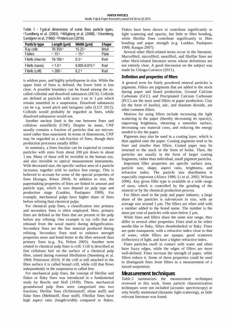
Table 1 - Typical dimensions of some fines particle types. a Sundberg et al. (2003). b Wågberg et al. (2008). c Steenberg, Sandgren et al. (1960) d Pettersson (2010). Particle type Length [µm] Width [µm] Shape Ray cells 70-350 a 15-25 a Brick Flakes ~ 15 a ~ 15 a Plate Fibrils (macro) 10-100 a 0.3 a Rod Fibrils (nano) < 1.0 b 0.005-0.015 b Rod Fibrils (crill) < 200 c 0.2 d Rod
is seldom pure, and highly polydisperse in size. While the upper limit of fines is defined, the lower limit is less clear. A possible boundary can be found among the so-called colloidal and dissolved substances (DCS). Colloids are defined as particles with sizes 1 nn to 1 µm which remain unsettled in a suspension. Dissolved substances can be e.g. wood pitch and inorganic salts (LUT 2012). Colloids would probably be regarded as fines, while dissolved substances would not.
Another unclear limit is the one between fines and cellulose nanofibrils (CNF). Despite its name, CNF usually contains a fraction of particles that are micron-sized rather than nanosized. In terms of dimensions, CNF may be regarded as a sub-fraction of fines, though their production processes usually differ.
In summary, a fines fraction can be expected to contain particles with sizes from about 200 µm down to about 1 nm. Many of these will be invisible to the human eye, and also invisible to optical measurement instruments. With decreased size, the specific surface area of a particle increases, together with its surface free energy. This is believed to account for some of the special properties of fines (Kangas, Kleen 2004). In addition to size, the papermaking properties of fines are linked to amount and particle type, which in turn depend on pulp type and production stage (Luukko, Paulapuro 1999). For example, mechanical pulps have higher share of fines before refining than chemical pulps.
For chemical pulp fines, a classification into primary and secondary fines is often employed. Here, primary fines are defined as the fines that are present in the pulp before any refining. One example is ray cells that are released from the wood matrix during delignification. Secondary fines are the fine material produced during refining. Secondary fines tend to enhance strength properties more and bond better in the fibre network than primary fines (e.g. Xu, Pelton 2005). Another term related to chemical pulp fines is crill. Crill is described as fine cellulosic hair on the surface of a chemical pulp fibre, raised during external fibrillation (Steenberg et al. 1960; Pettersson 2010). If the crill is still attached to the fibre surface it is called bound crill, while crill that flows independently in the suspension is called free.
For mechanical pulp fines, the concept of fibrillar and flakes or flaky fines was introduced in a fundamental study by Brecht and Holl (1939). There, mechanical groundwood pulp fines were categorized into two fractions; fibrillar fines (Schleimstoff, slime stuff) and flake fines (Mehlstoff, flour stuff). Fibrillar fines have high aspect ratio (length/width) compared to flakes.
Flakes have been shown to contribute significantly to light scattering and opacity, but little to fibre bonding, while fibrillar fines contribute significantly to fibre bonding and paper strength (e.g. Luukko, Paulapuro 1999; Kangas 2007).
Several other fibril-related terms occur in the literature. Macrofibril, microfibril, nanofibril, and fibrillar fines are other fibril-related literature terms whose definitions are not entirely clear. A good discussion on the subject was made by Chinga-Carrasco (2011).
Definition and properties of fillers A general term for finely powdered mineral particles is pigments. Fillers are pigments that are added to the stock during paper and board production. Ground Calcium Carbonate (GCC) and Precipitated Calcium Carbonate (PCC) are the most used fillers in paper production. Clay (in the form of kaolin), talc, and titanium dioxide, are other common fillers.
Motives for using fillers include increasing the light scattering in the paper (thereby decreasing its opacity), improving brightness, obtaining a smoother surface, decreasing raw material costs, and reducing the energy needed to dry the paper.
Pigments may also be used in a coating layer, which is then applied onto the paper. Coating pigments tend to be finer and smaller than fillers. Coated paper may be returned to the stock in the form of broke. Then, the particles are usually in the form of larger coating fragments, rather than individual, small pigment particles.
Important filler properties are specific surface area, particle size, shape, aspect ratio, brightness, and refractive index. The particle size distribution is especially important (Alince 1986; Li et al. 2002; Wilson 2006). Any given filler type is available in a wide range of sizes, which is controlled by the grinding of the mineral or by the chemical production process.
For fillers used in the pulp and paper industry, a large share of the particles is sub-micron in size, with an average size around 1 µm. The fillers are often sold with a number added to the brand name. The number is the mass per cent of particles with sizes below 2 µm.
While fines and fillers share the same size range, they differ in several other properties. Fines tend to be either needle-like or flaky, fillers rhombohedral or flaky. Fines are quite transparent, with a refractive index close to that of water, while fillers are opaque, good scatterers (reflectors) of light, and have a higher refractive index.
Fines particles swell in contact with water and often have fuzzy edges, while the edges of fillers are more well-defined. Fines increase the strength of paper, while fillers reduce it. Some of these properties could be used to distinguish fines from fillers in a measurement of a mixed suspension.
Measurement techniques Table 2 summarizes the measurement techniques reviewed in this work. Some particle characterization techniques were not included (acoustic spectroscopy) or only briefly mentioned (dynamic light scattering), as little relevant literature was found.
PAPER PHYSICS Nordic Pulp & Paper Research Journal Vol 30 no (3) 2015
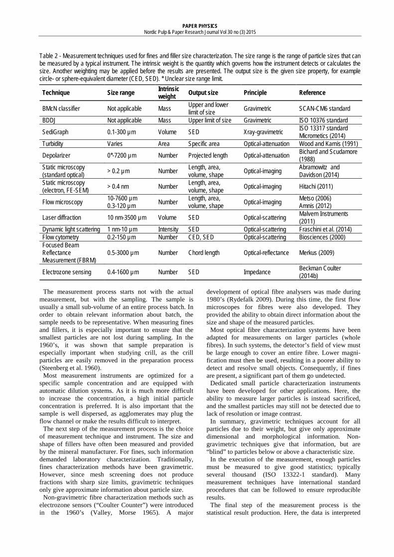
Table 2 - Measurement techniques used for fines and filler size characterization. The size range is the range of particle sizes that can be measured by a typical instrument. The intrinsic weight is the quantity which governs how the instrument detects or calculates the size. Another weighting may be applied before the results are presented. The output size is the given size property, for example circle- or sphere-equivalent diameter (CED, SED). * Unclear size range limit.
Technique Size range Intrinsic weight Output size Principle Reference
BMcN classifier Not applicable Mass Upper and lower limit of size Gravimetric SCAN-CM6 standard
BDDJ Not applicable Mass Upper limit of size Gravimetric ISO 10376 standard
SediGraph 0.1-300 µm Volume SED Xray-gravimetric ISO 13317 standard Micrometics (2014)
Turbidity Varies Area Specific area Optical-attenuation Wood and Karnis (1991)
Depolarizer 0*-7200 µm Number Projected length Optical-attenuation Bichard and Scudamore (1988)
Static microscopy (standard optical) > 0.2 µm Number Length, area,
volume, shape Optical-imaging Abramowitz and Davidson (2014)
Static microscopy (electron, FE-SEM) > 0.4 nm Number Length, area,
volume, shape Optical-imaging Hitachi (2011)
Flow microscopy 10-7600 µm
0.3-120 µm Number Length, area, volume, shape Optical-imaging Metso (2006)
Amnis (2012)
Laser diffraction 10 nm-3500 µm Volume SED Optical-scattering Malvern Instruments (2011)
Dynamic light scattering 1 nm-10 µm Intensity SED Optical-scattering Fraschini et al. (2014) Flow cytometry 0.2-150 µm Number CED, SED Optical-scattering Biosciences (2000) Focused Beam Reflectance Measurement (FBRM)
0.5-3000 µm Number Chord length Optical-reflectance Merkus (2009)
Electrozone sensing 0.4-1600 µm Number SED Impedance Beckman Coulter (2014b)
The measurement process starts not with the actual
measurement, but with the sampling. The sample is usually a small sub-volume of an entire process batch. In order to obtain relevant information about batch, the sample needs to be representative. When measuring fines and fillers, it is especially important to ensure that the smallest particles are not lost during sampling. In the 1960’s, it was shown that sample preparation is especially important when studying crill, as the crill particles are easily removed in the preparation process (Steenberg et al. 1960).
Most measurement instruments are optimized for a specific sample concentration and are equipped with automatic dilution systems. As it is much more difficult to increase the concentration, a high initial particle concentration is preferred. It is also important that the sample is well dispersed, as agglomerates may plug the flow channel or make the results difficult to interpret.
The next step of the measurement process is the choice of measurement technique and instrument. The size and shape of fillers have often been measured and provided by the mineral manufacturer. For fines, such information demanded laboratory characterization. Traditionally, fines characterization methods have been gravimetric. However, since mesh screening does not produce fractions with sharp size limits, gravimetric techniques only give approximate information about particle size.
Non-gravimetric fibre characterization methods such as electrozone sensors (“Coulter Counter”) were introduced in the 1960’s (Valley, Morse 1965). A major
development of optical fibre analysers was made during 1980’s (Rydefalk 2009). During this time, the first flow microscopes for fibres were also developed. They provided the ability to obtain direct information about the size and shape of the measured particles.
Most optical fibre characterization systems have been adapted for measurements on larger particles (whole fibres). In such systems, the detector’s field of view must be large enough to cover an entire fibre. Lower magni-fication must then be used, resulting in a poorer ability to detect and resolve small objects. Consequently, if fines are present, a significant part of them go undetected.
Dedicated small particle characterization instruments have been developed for other applications. Here, the ability to measure larger particles is instead sacrificed, and the smallest particles may still not be detected due to lack of resolution or image contrast.
In summary, gravimetric techniques account for all particles due to their weight, but give only approximate dimensional and morphological information. Non-gravimetric techniques give that information, but are “blind” to particles below or above a characteristic size.
In the execution of the measurement, enough particles must be measured to give good statistics; typically several thousand (ISO 13322-1 standard). Many measurement techniques have international standard procedures that can be followed to ensure reproducible results.
The final step of the measurement process is the statistical result production. Here, the data is interpreted

PAPER PHYSICS Nordic Pulp & Paper Research Journal Vol 30 no (3) 2015
by a statistical model; usually the log-normal probability distribution (ISO 9276-1 standard; Gregory 2005). Particle size distributions and average sizes are then calculated based on that model (e.g. ISO 9276-2 standard). For daily process control, average sizes may be sufficient, while research tasks may require the detailed information provided by a particle size distribution.
Most measurement techniques intrinsically emphasize a particular aspect of the sample; for example the number (amount) of particles, or their mass, volume, or length. The data is then said to be weighted in regard to that aspect (Pabst, Gregorova 2007; Malvern Instruments 2012). It is also possible to mathematically apply a weighting function to the data to convert it to a different weighting than that intrinsic to the measurement technique. When comparing measurement results on the same sample but from different instruments, it is important to have the same weighting on all data
Gravimetric techniques Gravimetric particle characterization can be coarsely grouped into screening techniques and sedimentation techniques. The former are most widely used in the pulp and paper industry, with instruments like the Bauer McNett classifier and the Britt Dynamic Drainage Jar.
In screening techniques, the pulp is sieved into a finer accept and a coarser reject, using a mesh or perforated screen. The passing accept fraction is usually designated as the P-fraction, e.g. P200. The rejected fraction is designated as the R-fraction, e.g. R200. The number is the mesh number, which corresponds to the number of threads per inch. As the mesh has some thickness, the actual opening size is slightly smaller. The shape of the opening, e.g. round or square, may also influence its actual size. In the pulp and paper industry, a 200-mesh usually corresponds to a 76 µm opening (equal to the definition of fines), while in ISO-standards, it corresponds to 75 µm. A table of mesh number vs. opening size for a selection of meshes is given in the Appendix.
The Bauer McNett classifier (BMcN) consists of a set of serial coupled chambers with screens of decreasing opening sizes (increasing mesh number). The shape of the mesh opening is square. The sample is poured into the first chamber and then passes through all stages. The particles caught in the respective fraction are weighted, and related to the initially added mass. The particles passing the finest mesh are typically not retained, as they are flushed away with the excess water (Rundlöf et al. 2000). For fibres, the screening is primarily done according to fibre length; the effects of fibre width are considered to be minor (Grahn, Björk 2013).
A critical parameter for the analysis is the duration of the analysis. In the flow, some longer particles may align vertically and pass the screens, creating overlapping size classes, see Fig 1 (Gooding, Olson 2001). This is especially true for pulp that has undergone bleaching and/or heavy refining. The amount of overlap increases with time, as particles get statistically more chances to align vertically against the mesh.
Fig 1 - Fibre length distribution of fractions from a BMcN classifier illustrating the overlap between the different fractions. The fibre length distribution was measured with a depolarizer (from Gooding and Olson 2001).
BMcN data is indicative of how much particle mass that can be found within a specific size span, for example between 53 µm and 76 µm for a P200/R300 fraction. However, direct size or shape data is not given; nor data on individual particles.
The Britt Dynamic Drainage Jar (BDDJ) is a single screen classifier. The names Dynamic Drainage Jar (DDJ) or, Britt Jar, are sometimes used to describe the same device. Typically, the screen is a perforated metal plate with round holes. The BDDJ separates the stock into a fibre fraction, retained on the screen, and a fines suspension. The standard size of the holes in a BDDJ screen is 76 µm (200-mesh), i.e. the passing fraction is identical to the definition of fines. Since no water is removed from the system, the fines suspension contains also the smallest fine material (Rundlöf et al. 2000). The BDDJ shares the BMcN’s susceptibility to fibre flexibility, i.e. the fines may also contain larger particles.
To determine the mass of the BDDJ fines, the suspension needs to be dewatered through a filter. The filter retention (pore) size is around 1.5 µm for a very fine quantitative paper filter, and around 0.7 µm for a microfiber glass filter (GE Healthcare 2014; Munktell 2014). Thus, it is possible that a share of small fines is lost, and hence unaccounted for in the weight. This possible error source is rarely discussed in the literature.
The SediGraph instrument (Micrometics Inc.) was introduced in 1967 and combines gravimetric sedimen-tation with x-ray absorption. The instrument can characterize particles that are opaque to X-rays, which include fillers but not lignocellulosic material (Wagner et al. 2007). In the SediGraph, the resolution of the X-rays, rather than the gravimetric sedimentation, determines the measurement range of the instrument, and some particles may thus be unaccounted for.
Other gravimetric pulp fractionation techniques which may indicate the size or shape of particles include sedimentation (e.g. Marton, Robie 1969), flow tubes (e.g. Laitinen et al. 2011), and hydrocyclones (e.g. Ullman et al. 1965).
Light attenuation and turbidity Several prototype instruments based on the attenuation (absorption and transmission) of light by a suspension have been developed. An often used parameter is the

PAPER PHYSICS Nordic Pulp & Paper Research Journal Vol 30 no (3) 2015
turbidity, i.e. the attenuation of light per unit depth in the suspension. A typical instrument illuminates a flowing suspension with one or more light beams with known properties (wavelength, intensity, beam size, etc.). A detector on the other side of the flow measures the changes in the transmitted light beam as it has passed through the flow. Individual particles are not characterized, as the measured data is the integrated response from all particles passing the beam. Physical theories and models are then used to relate the data to different particle properties, for example specific surface area (Wood, Karnis 1996).
An instrument may also utilize a combination of the attenuation and scattering of light, for example the Turbi-scan instrument from Formulaction (Holm, Manner 2001; 2003), and the OptoPlatform prototype instrument (Pettersson 2010). The OptoPlatform was recently commercialised as the CrillEye module to the PulpEye fibre analyser (Eurocon 2014). Depolarizer In the context of this review, a depolarizer is defined as an optical instrument which utilizes the birefringent properties of cellulose. Birefringence is the optical property of a material having a refractive index that depends on the polarization and propagation direction of light. Some filler minerals, e.g. calcium carbonate, also possess birefringence.
In the 1980’s, Kajaani introduced a commercial fibre analyser based on this principle; the FS-100. It was then considered a fast and simple instrument for fibre characterization (Bichard, Scudamore 1988). Its successor, the FS-200, will be used to illustrate the measurement technique.
In the FS-200, the fibres pass through a thin capillary channel. The capillary is illuminated by light, which passes a polarization filter to make it polarized. If
polarized light meets a fibre, its polarization changes. In front of the detector, the light has to pass a second filter, which lets through only the light that has met fibres in the capillary, and absorbs the rest. On the detector, the light projects an one-dimensional image proportional to the fibre length (Kaunonen, Luukkonen 1992). If the fibre is crooked, the projected length may be an underestimate of the true length (Hirn, Bauer 2006).
The output data is grouped into length classes at 50 µm intervals, starting at 0 µm. Imaging standards (ISO 16065-1) define fines as particles with size smaller than 200 µm. Hence, only four length classes are obtained in the fines range.
A “measurement sensitivity” of 5-10 µm has been stated for the FS-200 (Bichard, Scudamore 1988). However, it is unclear if this measurement sensitivity is the same as the resolution, e.g. the smallest particle that is included in the 0-50 µm range.
Today, depolarizers have largely been replaced by fibre analysers (flow microscopes).
Static microscopy Microscopy can be regarded as high-magnification imaging on static (fixed) particles. It can be used both qualitatively (manual inspection) or quantitatively (image analysis). To prepare a sample, a small amount of suspension is put onto a glass slide, which is referred to as the specimen. The specimen is then imaged with different illumination and detection techniques, see Fig 2.A-D) for examples. While not all of these techniques are encountered in the fines and filler literature, they give a basic insight into the capabilities of imaging.
Many of the microscopic techniques, or modes, improve contrast but not resolution. Contrast is the intensity difference between the particle and the background.
Resolution is the ability to resolve small image details.
Fig 2 - Static microscopy image of the same area of a fines-filler mix (courtsey of Joanna Hornatowska). A) Brightfield mode. B) Darkfield mode. C) Phase contrast mode. D) Differentical Interference Contrast (DIC) mode.
PAPER PHYSICS Nordic Pulp & Paper Research Journal Vol 30 no (3) 2015
The resolution can be varied through the optics (objective magnification), but is limited by the wavelength of the illuminated light. For visible light and tightly packed particles, the resolution limit is around 0.2 µm. With image analysis, it is sometimes possible to use gradients in the pixel values to obtain a higher efficient resolution, which is usually referred to as sub-pixel resolution.
The basic microscopic mode is brightfield, where the image is formed by the light transmitted through the specimen. For thin and transparent particles, brightfield mode may give insufficient contrast, see Fig 2A.
To increase contrast, the sample can be stained by fluorescent dyes. When a fluorescent dye is illuminated with suitable laser light, the specimen emits additional light, increasing the contrast. Using special fluorescent techniques known as super-resolution microscopy, the resolution may also be extended below the resolution limit. However, fluorescent staining may be time-consuming, impractical, and unselective (Hornatowska, Björk 2007; Rådberg 2010).
In darkfield mode, see Fig 2B, the reflected and scattered light from the specimen is gathered. Since the background does not contain any material that can reflect light, it appears dark. Darkfield mode highlights high-scattering particles, e.g. fillers.
In phase contrast mode, see Fig 2C, small differences in refractive index between the specimen and the surrounding medium are detected and translated to increased image contrast. The technique is especially useful for visualizing thin fibrils. However, the image may suffer from halos, i.e. artificial bright areas surrounding the particles. Additionally, phase contrast mode significantly reduces the depth of focus in the image. The depth-of-focus (or depth-of-field) is the range of distances in which the particle is in focus.
In polarized light mode, the birefringent properties of cellulose are utilized. When plane-polarized light interacts with the birefringent sample, it creates two individual wave components that are each polarized in mutually perpendicular planes. When these wave components pass a polarizer, they are recombined with constructive and destructive interference, which results in increased image contrast. An advantage of polarized light is that it does not significantly reduce the depth-of-focus of the image.
Differential Interference Contrast (DIC) mode, see Fig 2D, can be regarded as a modified polarized light microscope, where two prisms are added. In the technique, gradients in the optical path length of the sample are converted into amplitude differences that can be visualized as improved contrast in the resulting image. In DIC microscopy, objects are relief-like and seem to have a shadow cast.
Higher resolutions may be obtained by using e.g. shorter electromagnetic wavelengths, electron microscopy (scanning or transmission), or atomic force microscopy (AFM). Electron microscopy can reach resolutions better than 1 nm, making it one of the few available methods for the study of nanofibrils. However, electron microscopy is limited in the type of environment that can surround the sample. Vacuum or pure gas environment is typically
needed, rendering flowing (dynamic) setups impossible. Since the specimen preparation process is laborious, there are rarely enough imaged particles for reliable quantitative statistical analysis. Instead, electron microscopy is mainly used qualitatively.
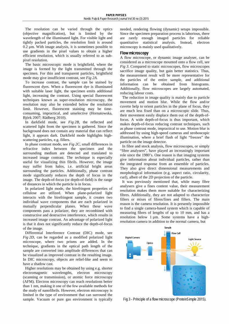
Flow microscopy A flow microscope, or dynamic image analyser, can be considered as a microscope mounted onto a flow cell, see Fig 3. Compared to static microscopes, flow microscopes sacrifice image quality, but gain better statistics. Thus, the measurement result will be more representative for the particles of the entire sample, and additional information can be obtained from histograms. Additionally, flow microscopes are largely automated, reducing labour costs.
The reduction in image quality is mainly due to particle movement and motion blur. While the flow and/or cuvette help to orient particles in the plane of focus, they are much less fixed than on a microscopic slide. Thus, their movement easily displace them out of the depth-of-focus. A wide depth-of-focus is thus important, which makes depth-of-focus reducing contrast techniques, such as phase contrast mode, impractical to use. Motion blur is addressed by using high-speed cameras and stroboscopic illumination, where a brief flash of light “freezes” the particle on the image detector.
In fibre and stock analysis, flow microscopes, or simply “fibre analysers”, have played an increasingly important role since the 1980’s. One reason is that imaging systems give information about individual particles, rather than the integrated response from an ensemble of particles. They also give direct dimensional measurements and morphological information (e.g. aspect ratio, circularity, curl), albeit of the 2D projection of the particle.
It was previously mentioned that, while many fibre analysers give a fines content value, their measurement resolution makes them more suitable for characterizing fibres. Additionally, they are not adapted to characterize fillers or mixes of fibres/fines and fillers. The main reason is the camera resolution. It is presently impossible to find a single camera-based system which is capable of measuring fibres of lengths of up to 10 mm, and has a resolution below 1 µm. Some systems have a high-resolution camera in addition to the normal camera, but
Fig 3 - Principle of a flow microscope (ProteinSimple 2015).
PAPER PHYSICS Nordic Pulp & Paper Research Journal Vol 30 no (3) 2015
the best resolution is still limited to around 1.5 x 1.5 µm2 per pixel (Hirn, Bauer 2006; Grahn, Björk 2013). As a large share of the filler and fines particles has at least one dimension smaller than 1 µm, many particles will not be detected and accounted for. Even if a particle is registered as a single pixel, it may be excluded from some calculations, as an area of at least 3x3 pixels is preferred for shape calculations.
While the lower size limit of the fines classification varies significantly between different instruments, the upper size limit is standardized. As previously mentioned, imaging standards classifies particles with length below 200 µm as fines, and particles above that as fibres. Some imaging systems also have aspect ratio critera, for example that a particle also must have aspect ratio > 4 in order to be classified as a fibre.
Since the typical resolution of a fibre analyser is around 10 µm, the fines content measured by most fibre analysers includes only particles with lengths between 10 and 200 µm. It should also be noted that the imaging definition of fines is quite different from the P76µm definition of the gravimetric standards. Thus, fines content obtained by imaging methods is not directly comparable to that obtained by gravimetric methods.
Polarized light is the only contrast technique that is commonly employed in fibre analysers, as it does not significantly decrease the depth-of-focus. Flow microscopes developed for other applications use a wider range of techniques to overcome resolution and contrast issues. Fluid Imaging’s FlowCam includes polarization and fluorescence options with a stated resolution of 1 µm (Fluid Imaging 2014). Amnis’ ImageStream uses hydro-dynamic focusing, fluorescence, and side-scattering, with a stated resolution of 0.33µm (Amnis 2012). Jasco’s IF-200nano uses monochromatic blue light illumination with a stated resolution of 0.2 µm (Jasco 2013). Still, there are limitations of imaging techniques that are difficult to overcome. Here, methods based on optical scattering offer an alternative.
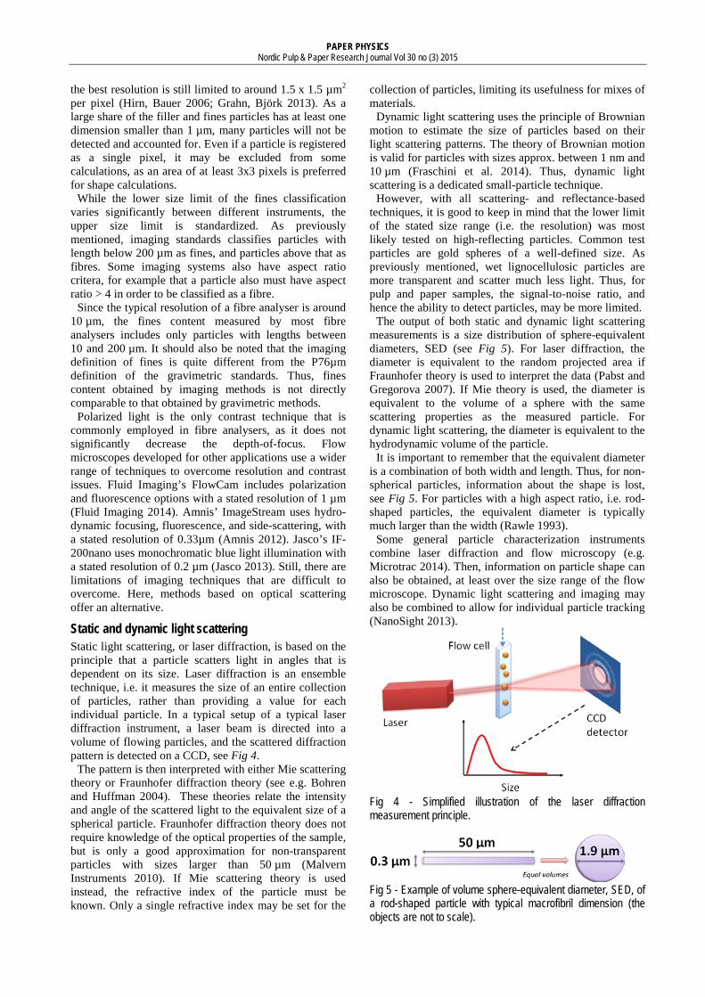
Static and dynamic light scattering Static light scattering, or laser diffraction, is based on the principle that a particle scatters light in angles that is dependent on its size. Laser diffraction is an ensemble technique, i.e. it measures the size of an entire collection of particles, rather than providing a value for each individual particle. In a typical setup of a typical laser diffraction instrument, a laser beam is directed into a volume of flowing particles, and the scattered diffraction pattern is detected on a CCD, see Fig 4.
The pattern is then interpreted with either Mie scattering theory or Fraunhofer diffraction theory (see e.g. Bohren and Huffman 2004). These theories relate the intensity and angle of the scattered light to the equivalent size of a spherical particle. Fraunhofer diffraction theory does not require knowledge of the optical properties of the sample, but is only a good approximation for non-transparent particles with sizes larger than 50 µm (Malvern Instruments 2010). If Mie scattering theory is used instead, the refractive index of the particle must be known. Only a single refractive index may be set for the
collection of particles, limiting its usefulness for mixes of materials.
Dynamic light scattering uses the principle of Brownian motion to estimate the size of particles based on their light scattering patterns. The theory of Brownian motion is valid for particles with sizes approx. between 1 nm and 10 µm (Fraschini et al. 2014). Thus, dynamic light scattering is a dedicated small-particle technique.
However, with all scattering- and reflectance-based techniques, it is good to keep in mind that the lower limit of the stated size range (i.e. the resolution) was most likely tested on high-reflecting particles. Common test particles are gold spheres of a well-defined size. As previously mentioned, wet lignocellulosic particles are more transparent and scatter much less light. Thus, for pulp and paper samples, the signal-to-noise ratio, and hence the ability to detect particles, may be more limited.
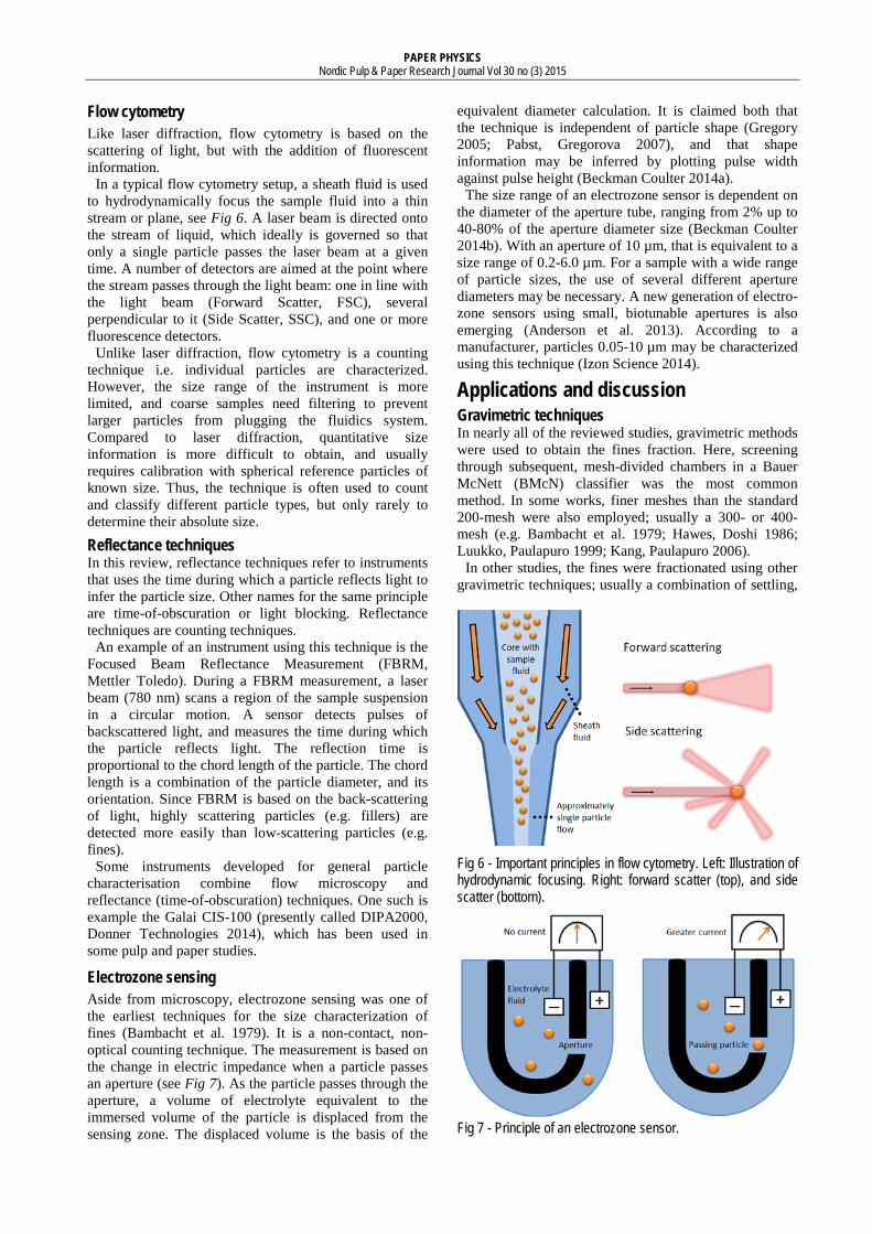
The output of both static and dynamic light scattering measurements is a size distribution of sphere-equivalent diameters, SED (see Fig 5). For laser diffraction, the diameter is equivalent to the random projected area if Fraunhofer theory is used to interpret the data (Pabst and Gregorova 2007). If Mie theory is used, the diameter is equivalent to the volume of a sphere with the same scattering properties as the measured particle. For dynamic light scattering, the diameter is equivalent to the hydrodynamic volume of the particle.
It is important to remember that the equivalent diameter is a combination of both width and length. Thus, for non-spherical particles, information about the shape is lost, see Fig 5. For particles with a high aspect ratio, i.e. rod-shaped particles, the equivalent diameter is typically much larger than the width (Rawle 1993).
Some general particle characterization instruments combine laser diffraction and flow microscopy (e.g. Microtrac 2014). Then, information on particle shape can also be obtained, at least over the size range of the flow microscope. Dynamic light scattering and imaging may also be combined to allow for individual particle tracking (NanoSight 2013).
Fig 4 - Simplified illustration of the laser diffraction measurement principle.
Fig 5 - Example of volume sphere-equivalent diameter, SED, of a rod-shaped particle with typical macrofibril dimension (the objects are not to scale).
PAPER PHYSICS Nordic Pulp & Paper Research Journal Vol 30 no (3) 2015
Flow cytometry Like laser diffraction, flow cytometry is based on the scattering of light, but with the addition of fluorescent information.
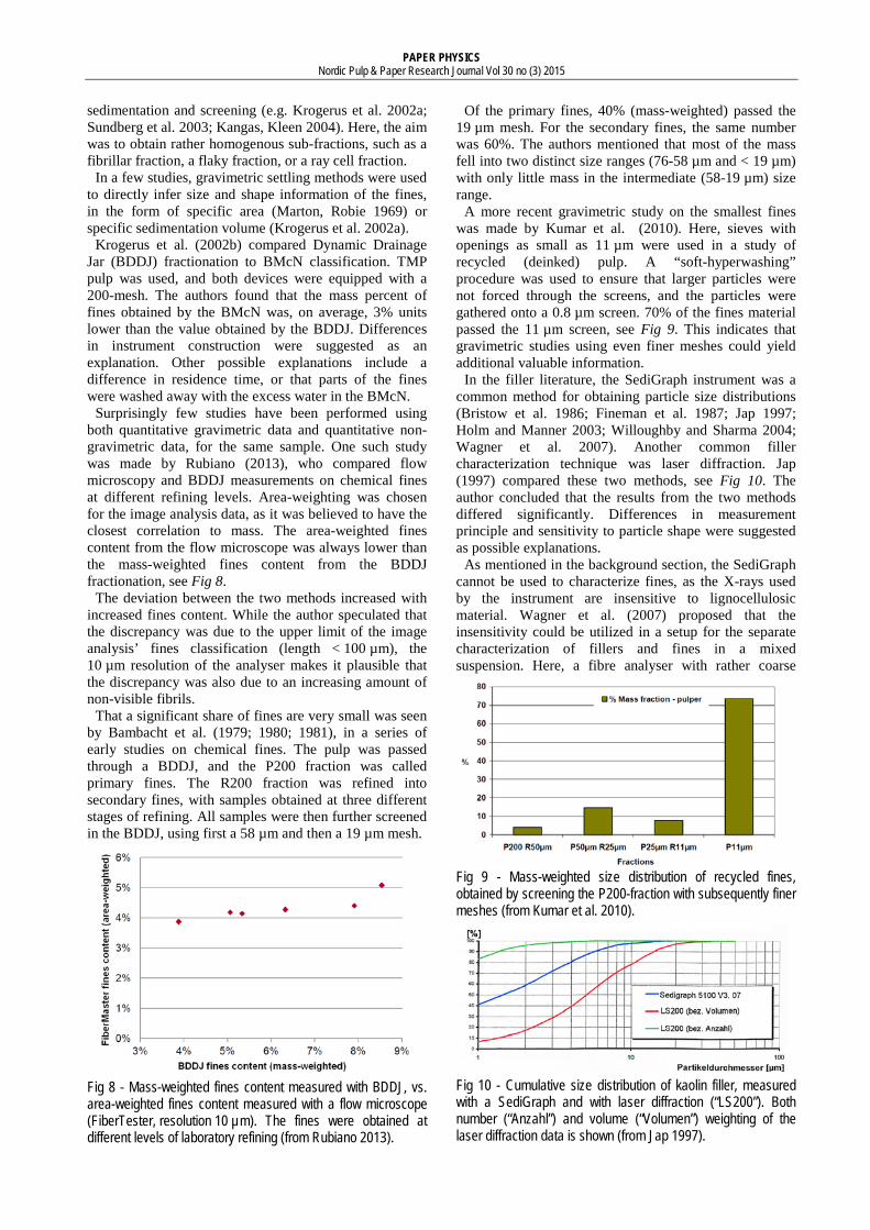
In a typical flow cytometry setup, a sheath fluid is used to hydrodynamically focus the sample fluid into a thin stream or plane, see Fig 6. A laser beam is directed onto the stream of liquid, which ideally is governed so that only a single particle passes the laser beam at a given time. A number of detectors are aimed at the point where the stream passes through the light beam: one in line with the light beam (Forward Scatter, FSC), several perpendicular to it (Side Scatter, SSC), and one or more fluorescence detectors.
Unlike laser diffraction, flow cytometry is a counting technique i.e. individual particles are characterized. However, the size range of the instrument is more limited, and coarse samples need filtering to prevent larger particles from plugging the fluidics system. Compared to laser diffraction, quantitative size information is more difficult to obtain, and usually requires calibration with spherical reference particles of known size. Thus, the technique is often used to count and classify different particle types, but only rarely to determine their absolute size.
Reflectance techniques In this review, reflectance techniques refer to instruments that uses the time during which a particle reflects light to infer the particle size. Other names for the same principle are time-of-obscuration or light blocking. Reflectance techniques are counting techniques.
An example of an instrument using this technique is the Focused Beam Reflectance Measurement (FBRM, Mettler Toledo). During a FBRM measurement, a laser beam (780 nm) scans a region of the sample suspension in a circular motion. A sensor detects pulses of backscattered light, and measures the time during which the particle reflects light. The reflection time is proportional to the chord length of the particle. The chord length is a combination of the particle diameter, and its orientation. Since FBRM is based on the back-scattering of light, highly scattering particles (e.g. fillers) are detected more easily than low-scattering particles (e.g. fines).
Some instruments developed for general particle characterisation combine flow microscopy and reflectance (time-of-obscuration) techniques. One such is example the Galai CIS-100 (presently called DIPA2000, Donner Technologies 2014), which has been used in some pulp and paper studies.
Electrozone sensing Aside from microscopy, electrozone sensing was one of the earliest techniques for the size characterization of fines (Bambacht et al. 1979). It is a non-contact, non-optical counting technique. The measurement is based on the change in electric impedance when a particle passes an aperture (see Fig 7). As the particle passes through the aperture, a volume of electrolyte equivalent to the immersed volume of the particle is displaced from the sensing zone. The displaced volume is the basis of the
equivalent diameter calculation. It is claimed both that the technique is independent of particle shape (Gregory 2005; Pabst, Gregorova 2007), and that shape information may be inferred by plotting pulse width against pulse height (Beckman Coulter 2014a).
The size range of an electrozone sensor is dependent on the diameter of the aperture tube, ranging from 2% up to 40-80% of the aperture diameter size (Beckman Coulter 2014b). With an aperture of 10 µm, that is equivalent to a size range of 0.2-6.0 µm. For a sample with a wide range of particle sizes, the use of several different aperture diameters may be necessary. A new generation of electro-zone sensors using small, biotunable apertures is also emerging (Anderson et al. 2013). According to a manufacturer, particles 0.05-10 µm may be characterized using this technique (Izon Science 2014).
Applications and discussion Gravimetric techniques In nearly all of the reviewed studies, gravimetric methods were used to obtain the fines fraction. Here, screening through subsequent, mesh-divided chambers in a Bauer McNett (BMcN) classifier was the most common method. In some works, finer meshes than the standard 200-mesh were also employed; usually a 300- or 400-mesh (e.g. Bambacht et al. 1979; Hawes, Doshi 1986; Luukko, Paulapuro 1999; Kang, Paulapuro 2006).
In other studies, the fines were fractionated using other gravimetric techniques; usually a combination of settling,
Fig 6 - Important principles in flow cytometry. Left: Illustration of hydrodynamic focusing. Right: forward scatter (top), and side scatter (bottom).
Fig 7 - Principle of an electrozone sensor.
PAPER PHYSICS Nordic Pulp & Paper Research Journal Vol 30 no (3) 2015
sedimentation and screening (e.g. Krogerus et al. 2002a; Sundberg et al. 2003; Kangas, Kleen 2004). Here, the aim was to obtain rather homogenous sub-fractions, such as a fibrillar fraction, a flaky fraction, or a ray cell fraction.
In a few studies, gravimetric settling methods were used to directly infer size and shape information of the fines, in the form of specific area (Marton, Robie 1969) or specific sedimentation volume (Krogerus et al. 2002a).
Krogerus et al. (2002b) compared Dynamic Drainage Jar (BDDJ) fractionation to BMcN classification. TMP pulp was used, and both devices were equipped with a 200-mesh. The authors found that the mass percent of fines obtained by the BMcN was, on average, 3% units lower than the value obtained by the BDDJ. Differences in instrument construction were suggested as an explanation. Other possible explanations include a difference in residence time, or that parts of the fines were washed away with the excess water in the BMcN.
Surprisingly few studies have been performed using both quantitative gravimetric data and quantitative non-gravimetric data, for the same sample. One such study was made by Rubiano (2013), who compared flow microscopy and BDDJ measurements on chemical fines at different refining levels. Area-weighting was chosen for the image analysis data, as it was believed to have the closest correlation to mass. The area-weighted fines content from the flow microscope was always lower than the mass-weighted fines content from the BDDJ fractionation, see Fig 8.
The deviation between the two methods increased with increased fines content. While the author speculated that the discrepancy was due to the upper limit of the image analysis’ fines classification (length < 100 µm), the 10 µm resolution of the analyser makes it plausible that the discrepancy was also due to an increasing amount of non-visible fibrils.
That a significant share of fines are very small was seen by Bambacht et al. (1979; 1980; 1981), in a series of early studies on chemical fines. The pulp was passed through a BDDJ, and the P200 fraction was called primary fines. The R200 fraction was refined into secondary fines, with samples obtained at three different stages of refining. All samples were then further screened in the BDDJ, using first a 58 µm and then a 19 µm mesh.
Fig 8 - Mass-weighted fines content measured with BDDJ, vs. area-weighted fines content measured with a flow microscope (FiberTester, resolution 10 µm). The fines were obtained at different levels of laboratory refining (from Rubiano 2013).
Of the primary fines, 40% (mass-weighted) passed the 19 µm mesh. For the secondary fines, the same number was 60%. The authors mentioned that most of the mass fell into two distinct size ranges (76-58 µm and < 19 µm) with only little mass in the intermediate (58-19 µm) size range.
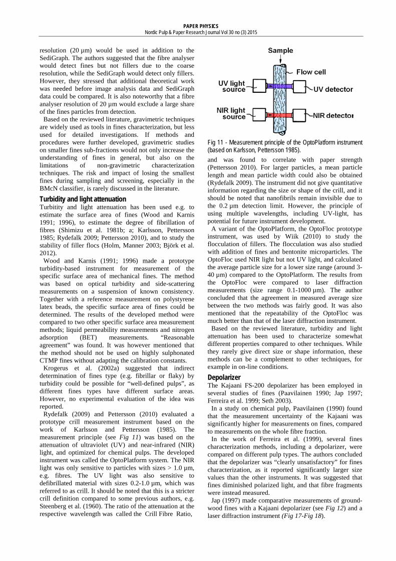
A more recent gravimetric study on the smallest fines was made by Kumar et al. (2010). Here, sieves with openings as small as 11 µm were used in a study of recycled (deinked) pulp. A “soft-hyperwashing” procedure was used to ensure that larger particles were not forced through the screens, and the particles were gathered onto a 0.8 µm screen. 70% of the fines material passed the 11 µm screen, see Fig 9. This indicates that gravimetric studies using even finer meshes could yield additional valuable information.
In the filler literature, the SediGraph instrument was a common method for obtaining particle size distributions (Bristow et al. 1986; Fineman et al. 1987; Jap 1997; Holm and Manner 2003; Willoughby and Sharma 2004; Wagner et al. 2007). Another common filler characterization technique was laser diffraction. Jap (1997) compared these two methods, see Fig 10. The author concluded that the results from the two methods differed significantly. Differences in measurement principle and sensitivity to particle shape were suggested as possible explanations.
As mentioned in the background section, the SediGraph cannot be used to characterize fines, as the X-rays used by the instrument are insensitive to lignocellulosic material. Wagner et al. (2007) proposed that the insensitivity could be utilized in a setup for the separate characterization of fillers and fines in a mixed suspension. Here, a fibre analyser with rather coarse
Fig 9 - Mass-weighted size distribution of recycled fines, obtained by screening the P200-fraction with subsequently finer meshes (from Kumar et al. 2010).
Fig 10 - Cumulative size distribution of kaolin filler, measured with a SediGraph and with laser diffraction (“LS200”). Both number (“Anzahl”) and volume (“Volumen”) weighting of the laser diffraction data is shown (from Jap 1997).
PAPER PHYSICS Nordic Pulp & Paper Research Journal Vol 30 no (3) 2015
resolution (20 µm) would be used in addition to the SediGraph. The authors suggested that the fibre analyser would detect fines but not fillers due to the coarse resolution, while the SediGraph would detect only fillers. However, they stressed that additional theoretical work was needed before image analysis data and SediGraph data could be compared. It is also noteworthy that a fibre analyser resolution of 20 µm would exclude a large share of the fines particles from detection.
Based on the reviewed literature, gravimetric techniques are widely used as tools in fines characterization, but less used for detailed investigations. If methods and procedures were further developed, gravimetric studies on smaller fines sub-fractions would not only increase the understanding of fines in general, but also on the limitations of non-gravimetric characterization techniques. The risk and impact of losing the smallest fines during sampling and screening, especially in the BMcN classifier, is rarely discussed in the literature.
Turbidity and light attenuation Turbitity and light attenuation has been used e.g. to estimate the surface area of fines (Wood and Karnis 1991; 1996), to estimate the degree of fibrillation of fibres (Shimizu et al. 1981b; a; Karlsson, Pettersson 1985; Rydefalk 2009; Pettersson 2010), and to study the stability of filler flocs (Holm, Manner 2003; Björk et al. 2012).
Wood and Karnis (1991; 1996) made a prototype turbidity-based instrument for measurement of the specific surface area of mechanical fines. The method was based on optical turbidity and side-scattering measurements on a suspension of known consistency. Together with a reference measurement on polystyrene latex beads, the specific surface area of fines could be determined. The results of the developed method were compared to two other specific surface area measurement methods; liquid permeability measurements and nitrogen adsorption (BET) measurements. “Reasonable agreement” was found. It was however mentioned that the method should not be used on highly sulphonated CTMP fines without adapting the calibration constants.
Krogerus et al. (2002a) suggested that indirect determination of fines type (e.g. fibrillar or flaky) by turbidity could be possible for “well-defined pulps”, as different fines types have different surface areas. However, no experimental evaluation of the idea was reported.
Rydefalk (2009) and Pettersson (2010) evaluated a prototype crill measurement instrument based on the work of Karlsson and Pettersson (1985). The measurement principle (see Fig 11) was based on the attenuation of ultraviolet (UV) and near-infrared (NIR) light, and optimized for chemical pulps. The developed instrument was called the OptoPlatform system. The NIR light was only sensitive to particles with sizes > 1.0 µm, e.g. fibres. The UV light was also sensitive to defibrillated material with sizes 0.2-1.0 µm, which was referred to as crill. It should be noted that this is a stricter crill definition compared to some previous authors, e.g. Steenberg et al. (1960). The ratio of the attenuation at the respective wavelength was called the Crill Fibre Ratio,
Fig 11 - Measurement principle of the OptoPlatform instrument (based on Karlsson, Pettersson 1985). and was found to correlate with paper strength (Pettersson 2010). For larger particles, a mean particle length and mean particle width could also be obtained (Rydefalk 2009). The instrument did not give quantitative information regarding the size or shape of the crill, and it should be noted that nanofibrils remain invisible due to the 0.2 µm detection limit. However, the principle of using multiple wavelengths, including UV-light, has potential for future instrument development.
A variant of the OptoPlatform, the OptoFloc prototype instrument, was used by Wiik (2010) to study the flocculation of fillers. The flocculation was also studied with addition of fines and bentonite microparticles. The OptoFloc used NIR light but not UV light, and calculated the average particle size for a lower size range (around 3-40 µm) compared to the OptoPlatform. The results from the OptoFloc were compared to laser diffraction measurements (size range 0.1-1000 µm). The author concluded that the agreement in measured average size between the two methods was fairly good. It was also mentioned that the repeatability of the OptoFloc was much better than that of the laser diffraction instrument.
Based on the reviewed literature, turbidity and light attenuation has been used to characterize somewhat different properties compared to other techniques. While they rarely give direct size or shape information, these methods can be a complement to other techniques, for example in on-line conditions.
Depolarizer The Kajaani FS-200 depolarizer has been employed in several studies of fines (Paavilainen 1990; Jap 1997; Ferreira et al. 1999; Seth 2003).
In a study on chemical pulp, Paavilainen (1990) found that the measurement uncertainty of the Kajaani was significantly higher for measurements on fines, compared to measurements on the whole fibre fraction.
In the work of Ferreira et al. (1999), several fines characterization methods, including a depolarizer, were compared on different pulp types. The authors concluded that the depolarizer was “clearly unsatisfactory” for fines characterization, as it reported significantly larger size values than the other instruments. It was suggested that fines diminished polarized light, and that fibre fragments were instead measured.
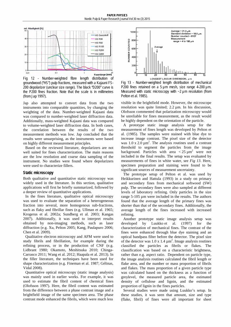
Jap (1997) made comparative measurements of ground-wood fines with a Kajaani depolarizer (see Fig 12) and a laser diffraction instrument (Fig 17-Fig 18).
PAPER PHYSICS Nordic Pulp & Paper Research Journal Vol 30 no (3) 2015
Fig 12 - Number-weighted fibre length distribution of groundwood (“HS”) pulp fractions, measured with a Kajaani FS-200 depolarizer (unclear size range). The black “D200” curve is the P200 fines fraction. Note that the scale is in millimetres (from Jap 1997).
Jap also attempted to convert data from the two instruments into comparable quantities, by changing the weighting of the data. Number-weighted Kajaani data was compared to number-weighted laser diffraction data. Additionally, mass-weighted Kajaani data was compared to volume-weighted laser diffraction data. In both cases, the correlation between the results of the two measurement methods was low. Jap concluded that the results were unsurprising, as the instruments were based on highly different measurement principles.
Based on the reviewed literature, depolarizers are not well suited for fines characterization. The main reasons are the low resolution and coarse data sampling of the instrument. No studies were found where depolarizers were used to characterize fillers.
Static microscopy Both qualitative and quantitative static microscopy was widely used in the literature. In this section, qualitative applications will first be briefly summarized, followed by a deeper review of quantitative applications.
In the fines literature, qualitative optical microscopy was used to evaluate the separation of a heterogeneous fraction into several, more homogenous sub-fractions, such as flaky and fibrillar fines (e.g. Ullman et al. 1965; Krogerus et al. 2002a; Sundberg et al. 2003; Kangas 2007). Additionally, it was used to interpret results obtained by non-imaging methods, such as laser diffraction (e.g. Xu, Pelton 2005; Kang, Paulapuro 2006; Chen et al. 2009).
Qualitative electron microscopy and AFM were used to study fibrils and fibrillation, for example during the refining process, or in the production of CNF (e.g. Lidbrant 1980; Okamoto, Meshitsuka 2010; Chinga-Carrasco 2011; Wang et al. 2012; Haapala et al. 2013). In the filler literature, the techniques have been used for shape characterization (e.g. Fineman et al. 1987; Gélinas, Vidal 2008).
Quantitative optical microscopy (static image analysis) was mainly used in earlier works. For example, it was used to estimate the fibril content of chemical fines (Olofsson 1997). Here, the fibril content was estimated from the difference between a phase contrast image and a brightfield image of the same specimen area. The phase contrast mode enhanced the fibrils, which were much less
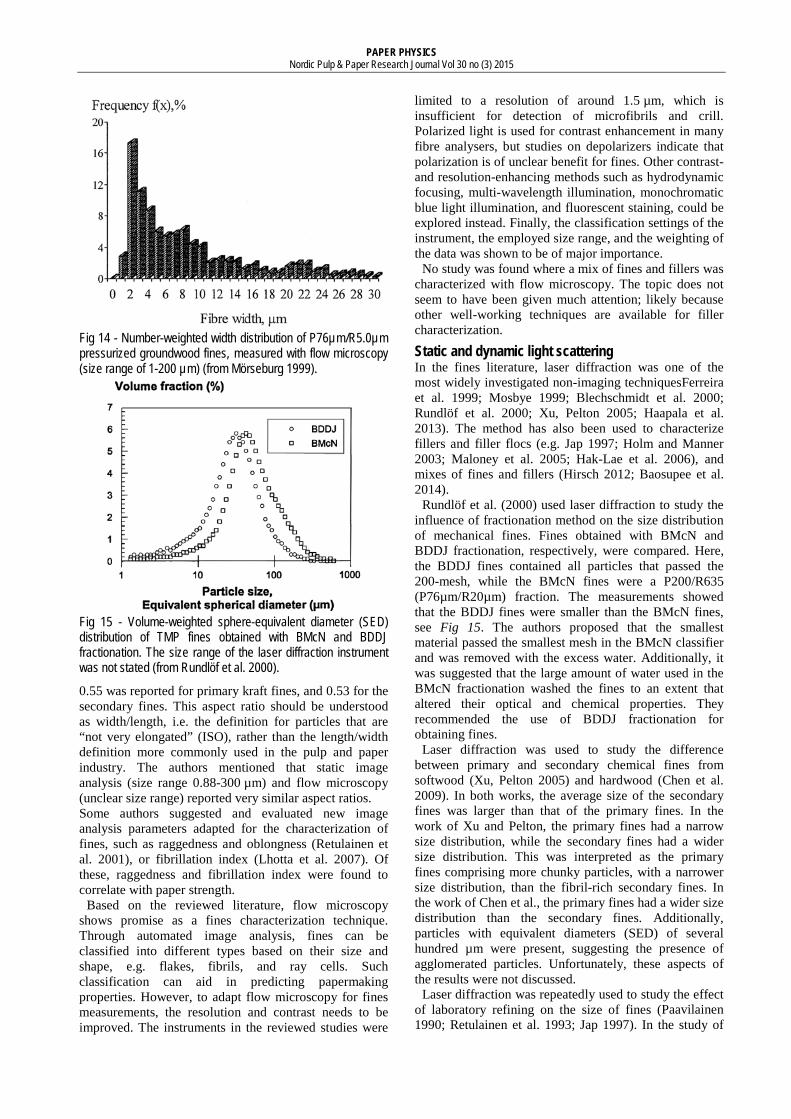
Fig 13 - Number-weighted length distribution of mechanical P200 fines retained on a 5 µm mesh, size range 4-200 µm. Measured with static microscopy with ~2 µm resolution (from Pelton et al. 1985). visible in the brightfield mode. However, the microscope resolution was quite limited; 2.2 µm. In his discussion, Olofsson commented that polarization microscopy would be unreliable for fines measurement, as the result would be highly dependent on the orientation of the particle.
A prototype static image analysis setup for the measurement of fines length was developed by Pelton et al. (1985). The samples were stained with blue dye to increase image contrast. The pixel size of the detector was 1.0 x 2.0 µm2. The analysis routines used a contrast threshold to segment the particles from the image background. Particles with area < 25 µm2 were not included in the final results. The setup was evaluated by measurements of fines in white water, see Fig 13. Here, specimen preparation and staining were found to be significant sources of measurement uncertainty.
The prototype setup of Pelton et al. was used by Heikkurinen and Hattula (1993) in a study on primary and secondary fines from mechanical softwood (SW) pulp. The secondary fines were also sampled at different levels of laboratory refining. Only particles in the size range 5-105 µm were included in the results. The authors found that the average length of the primary fines was shorter than that of the secondary fines. Additionally, the average length of the fines increased with increased refining.
Another prototype static image analysis setup was developed by Luukko et al. (1997) for the characterization of mechanical fines. The contrast of the fines were enhanced through blue dye staining and an optical bandpass filter before the detector. The pixel size of the detector was 1.0 x 1.4 µm2. Image analysis routines classified the particles as fibrils or flakes. The classification was based on a characteristic brightness, rather than e.g. aspect ratio. Dependent on particle type, the image analysis routines calculated the fibril length or flake area, and the number or mass proportion of fibrils and flakes. The mass proportion of a given particle type was calculated based on the thickness as a function of greylevel, the measured particle area, the estimated density of cellulose and lignin, and the estimated proportion of lignin in the fines particles.
Several studies were made using Luukko’s setup. In these studies, it was seen that amount, size and type (flake, fibril) of fines were all important for sheet

PAPER PHYSICS Nordic Pulp & Paper Research Journal Vol 30 no (3) 2015
properties (Luukko 1999; Luukko, Paulapuro 1999). In one study, SW TMP fines were measured at different refining levels of laboratory refining (Luukko et al. 1997). It was found that the fibril length decreased with increased refining, while the flake area showed no clear trend. The results appear to be contrary to those reported by Heikkurinen and Hattula (1993). A possible explanation is that the older study did not classify the fines into fibrils and flakes, whose length could have different development during refining.
Quantitative scanning electron microscopy (SEM) was used by Haapala et al. (2013) to characterize micro-fibrillar cellulose and other microsized wood-based particles. The authors concluded that automated analysis of the electron microscopy images was problematic, since the particles were often overlapping. It was mentioned that the structure of wet microfibrils is uncertain, due to the difficulty in measuring them in suspended phase. Other authors have mentioned that drying and swelling during specimen preparation and measurement may influence the measured size in ways that are not fully understood (Okamoto, Meshitsuka 2010). Furthermore, there was a lack of discussion in the reviewed electron microscopy studies on how surface charging artefacts could influence the measured sizes.
Quantitative atomic Force Microscopy (AFM) was used by Paiva et al. (2007) to characterize eucalypt kraft pulp. The authors concluded that it was possible to measure the diameters of what they referred to as macrofibrils (average diameter 0.66 μm) and microfibrils (average diameter 10-18 nm), and to resolve elementary cellulose fibrils. They mentioned that it was very difficult to estimate the fibril length, though a minimum length of 0.3 µm was stated. A likely explanation is that the fibrils were long enough to be partially outside the AFM image.
Based on the reviewed fines literature of qualitative and quantitative microscopy, qualitative microscopy is routinely used as an aid to interpret non-imaging characterization methods, for example gravimetric fractionation. Quantitative optical microscopy was mainly reported in early fines studies. Here, surprisingly coarse resolutions were used, and shape parameters were rarely reported. As the interest in fines and micro- and nanoscale fibrils have increased, quantitative electron microscopy and AFM have emerged as high-resolution alternatives. These techniques have also been used to study the shape of fillers. However, in microscopy in general and electron microscopy and AFM in particular, the data is often obtained from only one or a few images, as sample preparation and measurement are highly laborious. As only few images are used in the evaluation, the results are sensitive to sampling and sample preparation, and the statistical uncertainty is high. While static microscopy will see continued use as a high-resolution reference method, routine characterization of fines and fillers require more efficient methods.
Flow microscopy Flow microscopy has been employed in a wide range of fines studies. Many of the commercial fibre analysers give a fines content value, but do not give size or shape data on fines. In order to obtain such data, some authors
used prototype setups (e.g. Krogerus et al. 2002b; Kangas, Kleen 2004) or flow microscopes developed for other application areas (Ferreira et al. 1999; Mörseburg 1999).
Two studies compared fibre analysers by measuring on the same fines samples with different instruments (Guay et al. 2005; Grahn, Björk 2013). The trends in fines content were largely similar for the different analysers, but the absolute levels could vary significantly. As expected, a more stringent definition of fines (< 100 µm, instead of < 200 µm) gave lower fines content. The resolution of the instrument and the weighting of the data were also important. Grahn and Björk (2013) evaluated number-, length-, and area-weighting, and concluded that the fines content was highest with number (arithmetical) weighting, and lowest with area-weighting.
The prototype static image analysis setup of Luukko et al. (1997) was developed into a flow microscope and used by several authors (Retulainen et al. 2001; Krogerus et al. 2002a; Krogerus et al. 2002b; Sundberg et al. 2003; Kangas, Kleen 2004; Kangas 2007; Yin et al. 2013). The setup was later commercialized as the FiberLab fibre analyser (Rodrigues Alves 2011). The image analysis routines of the setup were adapted for the classification of ray cells, based on their brick-like shape (Krogerus et al. 2002b). However, the classification was mentioned to be in need of further development, as it often classified broken ray cells as flakes (Kangas, Kleen 2004).
The flowing version of Luukko’s setup had a size range of around 1.4-100 µm, as the flow cell diameter limited the maximum particle size. That this size range excludes thin as well as very long particles should be noted. Using SEM, Kangas and Kleen (2004) estimated that the width of their TMP fibrils was 0.05-1 µm. Simultaneously, they used Luukko’s setup to estimate the apparent mass proportion of fibrils in their samples to up to 84%. The fibrils would need to be at least 1.4 µm in width in order to be resolved by Luukko’s setup. These “thick fibrils” are seldom discussed in relation to macro- or microfibrils (see Table 1). In general, it is unclear at which length and width that fibrils start to lose their fines-specific properties, and approach the properties of fibres.
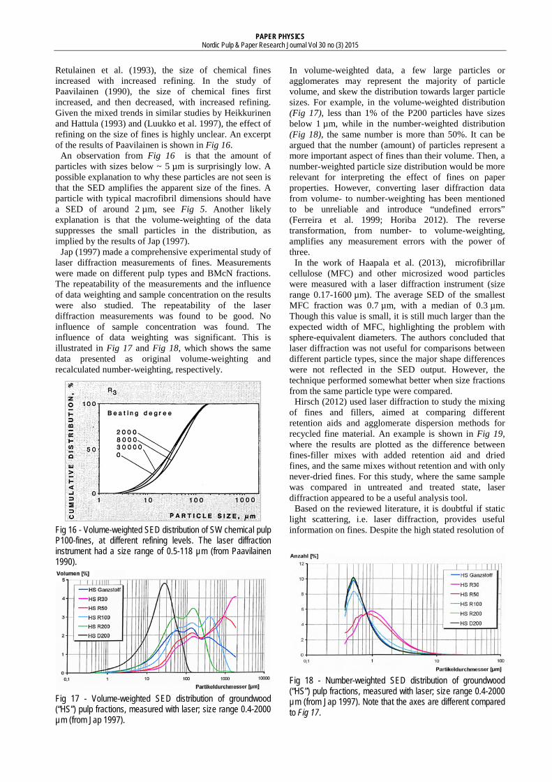
One of the few studies on the width of fines was made by Mörseburg (1999). Here, a flow microscope was used to measure the width distribution of groundwood P76µm/R5.0µm fines. The author defined three “fibre” classes based on the width; ribbons (width 1-5 µm), fragments (width 6-14 µm), and fibre residue (width > 14 µm). The fines were found to have high degree of ribbons, see Fig 14. In Fig 14, the combination of a low amount of material in the 1 µm size bin and a larger amount in the 2 µm bin is surprising, as the number of fines particles tend to increase with decreased size. Likely, the 1 µm resolution of the instrument was not enough to calculate reliable width data for 1 µm particles. Alternatively, the material in the 1 µm bin was too small in both width and length to be retained on the 5.0 µm mesh.
The width and length of fines was surprisingly rarely measured in the same study. Thus, only a single study was found where the aspect ratio of fines was reported (Ferreira et al. 1999). Here, an average aspect ratio of
PAPER PHYSICS Nordic Pulp & Paper Research Journal Vol 30 no (3) 2015
Fig 14 - Number-weighted width distribution of P76µm/R5.0µm pressurized groundwood fines, measured with flow microscopy (size range of 1-200 µm) (from Mörseburg 1999).
Fig 15 - Volume-weighted sphere-equivalent diameter (SED) distribution of TMP fines obtained with BMcN and BDDJ fractionation. The size range of the laser diffraction instrument was not stated (from Rundlöf et al. 2000).
0.55 was reported for primary kraft fines, and 0.53 for the secondary fines. This aspect ratio should be understood as width/length, i.e. the definition for particles that are “not very elongated” (ISO), rather than the length/width definition more commonly used in the pulp and paper industry. The authors mentioned that static image analysis (size range 0.88-300 µm) and flow microscopy (unclear size range) reported very similar aspect ratios. Some authors suggested and evaluated new image analysis parameters adapted for the characterization of fines, such as raggedness and oblongness (Retulainen et al. 2001), or fibrillation index (Lhotta et al. 2007). Of these, raggedness and fibrillation index were found to correlate with paper strength.
Based on the reviewed literature, flow microscopy shows promise as a fines characterization technique. Through automated image analysis, fines can be classified into different types based on their size and shape, e.g. flakes, fibrils, and ray cells. Such classification can aid in predicting papermaking properties. However, to adapt flow microscopy for fines measurements, the resolution and contrast needs to be improved. The instruments in the reviewed studies were
limited to a resolution of around 1.5 µm, which is insufficient for detection of microfibrils and crill. Polarized light is used for contrast enhancement in many fibre analysers, but studies on depolarizers indicate that polarization is of unclear benefit for fines. Other contrast- and resolution-enhancing methods such as hydrodynamic focusing, multi-wavelength illumination, monochromatic blue light illumination, and fluorescent staining, could be explored instead. Finally, the classification settings of the instrument, the employed size range, and the weighting of the data was shown to be of major importance.
No study was found where a mix of fines and fillers was characterized with flow microscopy. The topic does not seem to have been given much attention; likely because other well-working techniques are available for filler characterization.
Static and dynamic light scattering In the fines literature, laser diffraction was one of the most widely investigated non-imaging techniquesFerreira et al. 1999; Mosbye 1999; Blechschmidt et al. 2000; Rundlöf et al. 2000; Xu, Pelton 2005; Haapala et al. 2013). The method has also been used to characterize fillers and filler flocs (e.g. Jap 1997; Holm and Manner 2003; Maloney et al. 2005; Hak-Lae et al. 2006), and mixes of fines and fillers (Hirsch 2012; Baosupee et al. 2014).
Rundlöf et al. (2000) used laser diffraction to study the influence of fractionation method on the size distribution of mechanical fines. Fines obtained with BMcN and BDDJ fractionation, respectively, were compared. Here, the BDDJ fines contained all particles that passed the 200-mesh, while the BMcN fines were a P200/R635 (P76µm/R20µm) fraction. The measurements showed that the BDDJ fines were smaller than the BMcN fines, see Fig 15. The authors proposed that the smallest material passed the smallest mesh in the BMcN classifier and was removed with the excess water. Additionally, it was suggested that the large amount of water used in the BMcN fractionation washed the fines to an extent that altered their optical and chemical properties. They recommended the use of BDDJ fractionation for obtaining fines.
Laser diffraction was used to study the difference between primary and secondary chemical fines from softwood (Xu, Pelton 2005) and hardwood (Chen et al. 2009). In both works, the average size of the secondary fines was larger than that of the primary fines. In the work of Xu and Pelton, the primary fines had a narrow size distribution, while the secondary fines had a wider size distribution. This was interpreted as the primary fines comprising more chunky particles, with a narrower size distribution, than the fibril-rich secondary fines. In the work of Chen et al., the primary fines had a wider size distribution than the secondary fines. Additionally, particles with equivalent diameters (SED) of several hundred µm were present, suggesting the presence of agglomerated particles. Unfortunately, these aspects of the results were not discussed.
Laser diffraction was repeatedly used to study the effect of laboratory refining on the size of fines (Paavilainen 1990; Retulainen et al. 1993; Jap 1997). In the study of
PAPER PHYSICS Nordic Pulp & Paper Research Journal Vol 30 no (3) 2015
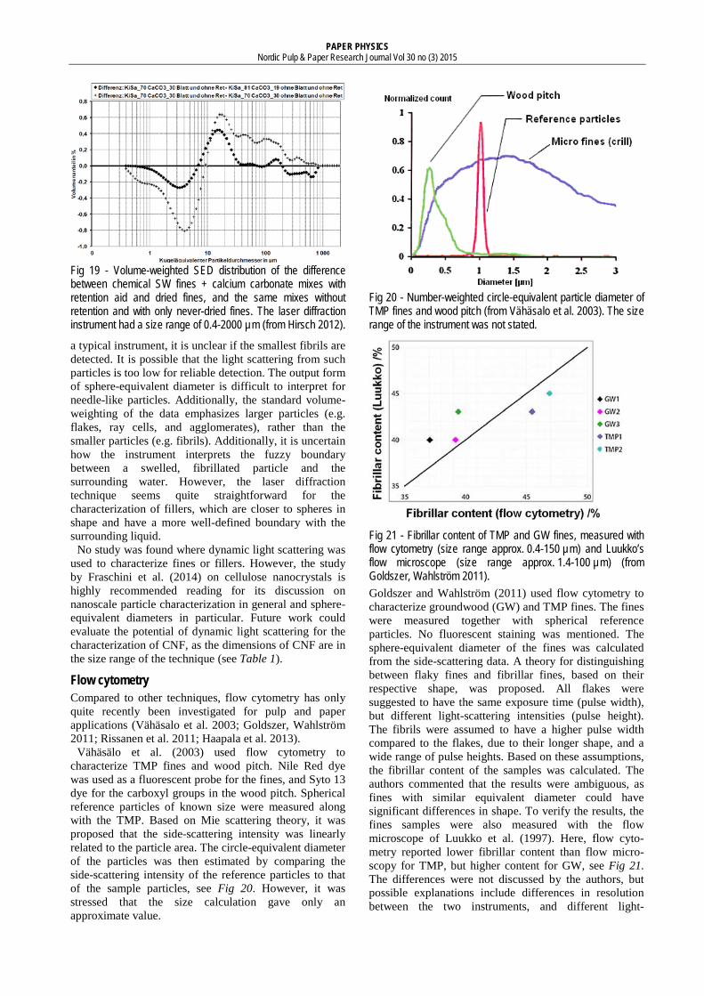
Retulainen et al. (1993), the size of chemical fines increased with increased refining. In the study of Paavilainen (1990), the size of chemical fines first increased, and then decreased, with increased refining. Given the mixed trends in similar studies by Heikkurinen and Hattula (1993) and (Luukko et al. 1997), the effect of refining on the size of fines is highly unclear. An excerpt of the results of Paavilainen is shown in Fig 16.
An observation from Fig 16 is that the amount of particles with sizes below ~ 5 µm is surprisingly low. A possible explanation to why these particles are not seen is that the SED amplifies the apparent size of the fines. A particle with typical macrofibril dimensions should have a SED of around 2 µm, see Fig 5. Another likely explanation is that the volume-weighting of the data suppresses the small particles in the distribution, as implied by the results of Jap (1997).
Jap (1997) made a comprehensive experimental study of laser diffraction measurements of fines. Measurements were made on different pulp types and BMcN fractions. The repeatability of the measurements and the influence of data weighting and sample concentration on the results were also studied. The repeatability of the laser diffraction measurements was found to be good. No influence of sample concentration was found. The influence of data weighting was significant. This is illustrated in Fig 17 and Fig 18, which shows the same data presented as original volume-weighting and recalculated number-weighting, respectively.
Fig 16 - Volume-weighted SED distribution of SW chemical pulp P100-fines, at different refining levels. The laser diffraction instrument had a size range of 0.5-118 µm (from Paavilainen 1990).
Fig 17 - Volume-weighted SED distribution of groundwood (“HS”) pulp fractions, measured with laser; size range 0.4-2000 µm (from Jap 1997).
In volume-weighted data, a few large particles or agglomerates may represent the majority of particle volume, and skew the distribution towards larger particle sizes. For example, in the volume-weighted distribution (Fig 17), less than 1% of the P200 particles have sizes below 1 µm, while in the number-weighted distribution (Fig 18), the same number is more than 50%. It can be argued that the number (amount) of particles represent a more important aspect of fines than their volume. Then, a number-weighted particle size distribution would be more relevant for interpreting the effect of fines on paper properties. However, converting laser diffraction data from volume- to number-weighting has been mentioned to be unreliable and introduce “undefined errors” (Ferreira et al. 1999; Horiba 2012). The reverse transformation, from number- to volume-weighting, amplifies any measurement errors with the power of three.
In the work of Haapala et al. (2013), microfibrillar cellulose (MFC) and other microsized wood particles were measured with a laser diffraction instrument (size range 0.17-1600 µm). The average SED of the smallest MFC fraction was 0.7 µm, with a median of 0.3 µm. Though this value is small, it is still much larger than the expected width of MFC, highlighting the problem with sphere-equivalent diameters. The authors concluded that laser diffraction was not useful for comparisons between different particle types, since the major shape differences were not reflected in the SED output. However, the technique performed somewhat better when size fractions from the same particle type were compared.
Hirsch (2012) used laser diffraction to study the mixing of fines and fillers, aimed at comparing different retention aids and agglomerate dispersion methods for recycled fine material. An example is shown in Fig 19, where the results are plotted as the difference between fines-filler mixes with added retention aid and dried fines, and the same mixes without retention and with only never-dried fines. For this study, where the same sample was compared in untreated and treated state, laser diffraction appeared to be a useful analysis tool.
Based on the reviewed literature, it is doubtful if static light scattering, i.e. laser diffraction, provides useful information on fines. Despite the high stated resolution of
Fig 18 - Number-weighted SED distribution of groundwood (“HS”) pulp fractions, measured with laser; size range 0.4-2000 µm (from Jap 1997). Note that the axes are different compared to Fig 17.
PAPER PHYSICS Nordic Pulp & Paper Research Journal Vol 30 no (3) 2015
Fig 19 - Volume-weighted SED distribution of the difference between chemical SW fines + calcium carbonate mixes with retention aid and dried fines, and the same mixes without retention and with only never-dried fines. The laser diffraction instrument had a size range of 0.4-2000 µm (from Hirsch 2012).
a typical instrument, it is unclear if the smallest fibrils are detected. It is possible that the light scattering from such particles is too low for reliable detection. The output form of sphere-equivalent diameter is difficult to interpret for needle-like particles. Additionally, the standard volume-weighting of the data emphasizes larger particles (e.g. flakes, ray cells, and agglomerates), rather than the smaller particles (e.g. fibrils). Additionally, it is uncertain how the instrument interprets the fuzzy boundary between a swelled, fibrillated particle and the surrounding water. However, the laser diffraction technique seems quite straightforward for the characterization of fillers, which are closer to spheres in shape and have a more well-defined boundary with the surrounding liquid.
No study was found where dynamic light scattering was used to characterize fines or fillers. However, the study by Fraschini et al. (2014) on cellulose nanocrystals is highly recommended reading for its discussion on nanoscale particle characterization in general and sphere-equivalent diameters in particular. Future work could evaluate the potential of dynamic light scattering for the characterization of CNF, as the dimensions of CNF are in the size range of the technique (see Table 1).
Flow cytometry Compared to other techniques, flow cytometry has only quite recently been investigated for pulp and paper applications (Vähäsalo et al. 2003; Goldszer, Wahlström 2011; Rissanen et al. 2011; Haapala et al. 2013).
Vähäsälo et al. (2003) used flow cytometry to characterize TMP fines and wood pitch. Nile Red dye was used as a fluorescent probe for the fines, and Syto 13 dye for the carboxyl groups in the wood pitch. Spherical reference particles of known size were measured along with the TMP. Based on Mie scattering theory, it was proposed that the side-scattering intensity was linearly related to the particle area. The circle-equivalent diameter of the particles was then estimated by comparing the side-scattering intensity of the reference particles to that of the sample particles, see Fig 20. However, it was stressed that the size calculation gave only an approximate value.
Fig 20 - Number-weighted circle-equivalent particle diameter of TMP fines and wood pitch (from Vähäsalo et al. 2003). The size range of the instrument was not stated.
Fig 21 - Fibrillar content of TMP and GW fines, measured with flow cytometry (size range approx. 0.4-150 µm) and Luukko’s flow microscope (size range approx. 1.4-100 µm) (from Goldszer, Wahlström 2011). Goldszer and Wahlström (2011) used flow cytometry to characterize groundwood (GW) and TMP fines. The fines were measured together with spherical reference particles. No fluorescent staining was mentioned. The sphere-equivalent diameter of the fines was calculated from the side-scattering data. A theory for distinguishing between flaky fines and fibrillar fines, based on their respective shape, was proposed. All flakes were suggested to have the same exposure time (pulse width), but different light-scattering intensities (pulse height). The fibrils were assumed to have a higher pulse width compared to the flakes, due to their longer shape, and a wide range of pulse heights. Based on these assumptions, the fibrillar content of the samples was calculated. The authors commented that the results were ambiguous, as fines with similar equivalent diameter could have significant differences in shape. To verify the results, the fines samples were also measured with the flow microscope of Luukko et al. (1997). Here, flow cyto-metry reported lower fibrillar content than flow micro-scopy for TMP, but higher content for GW, see Fig 21. The differences were not discussed by the authors, but possible explanations include differences in resolution between the two instruments, and different light-
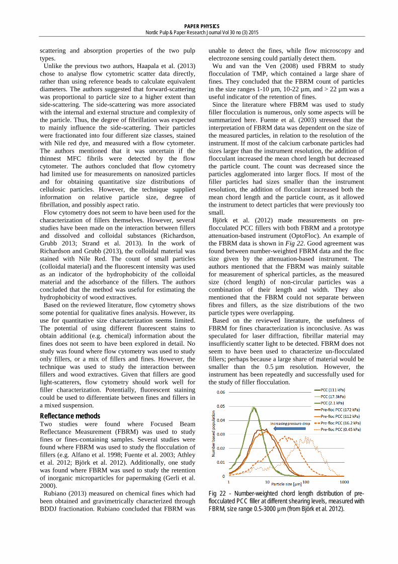
PAPER PHYSICS Nordic Pulp & Paper Research Journal Vol 30 no (3) 2015
scattering and absorption properties of the two pulp types.
Unlike the previous two authors, Haapala et al. (2013) chose to analyse flow cytometric scatter data directly, rather than using reference beads to calculate equivalent diameters. The authors suggested that forward-scattering was proportional to particle size to a higher extent than side-scattering. The side-scattering was more associated with the internal and external structure and complexity of the particle. Thus, the degree of fibrillation was expected to mainly influence the side-scattering. Their particles were fractionated into four different size classes, stained with Nile red dye, and measured with a flow cytometer. The authors mentioned that it was uncertain if the thinnest MFC fibrils were detected by the flow cytometer. The authors concluded that flow cytometry had limited use for measurements on nanosized particles and for obtaining quantitative size distributions of cellulosic particles. However, the technique supplied information on relative particle size, degree of fibrillation, and possibly aspect ratio.
Flow cytometry does not seem to have been used for the characterization of fillers themselves. However, several studies have been made on the interaction between fillers and dissolved and colloidal substances (Richardson, Grubb 2013; Strand et al. 2013). In the work of Richardson and Grubb (2013), the colloidal material was stained with Nile Red. The count of small particles (colloidal material) and the fluorescent intensity was used as an indicator of the hydrophobicity of the colloidal material and the adsorbance of the fillers. The authors concluded that the method was useful for estimating the hydrophobicity of wood extractives.
Based on the reviewed literature, flow cytometry shows some potential for qualitative fines analysis. However, its use for quantitative size characterization seems limited. The potential of using different fluorescent stains to obtain additional (e.g. chemical) information about the fines does not seem to have been explored in detail. No study was found where flow cytometry was used to study only fillers, or a mix of fillers and fines. However, the technique was used to study the interaction between fillers and wood extractives. Given that fillers are good light-scatterers, flow cytometry should work well for filler characterization. Potentially, fluorescent staining could be used to differentiate between fines and fillers in a mixed suspension.
Reflectance methods Two studies were found where Focused Beam Reflectance Measurement (FBRM) was used to study fines or fines-containing samples. Several studies were found where FBRM was used to study the flocculation of fillers (e.g. Alfano et al. 1998; Fuente et al. 2003; Athley et al. 2012; Björk et al. 2012). Additionally, one study was found where FBRM was used to study the retention of inorganic microparticles for papermaking (Gerli et al. 2000).
Rubiano (2013) measured on chemical fines which had been obtained and gravimetrically characterized through BDDJ fractionation. Rubiano concluded that FBRM was
unable to detect the fines, while flow microscopy and electrozone sensing could partially detect them.
Wu and van the Ven (2008) used FBRM to study flocculation of TMP, which contained a large share of fines. They concluded that the FBRM count of particles in the size ranges 1-10 µm, 10-22 µm, and > 22 µm was a useful indicator of the retention of fines.
Since the literature where FBRM was used to study filler flocculation is numerous, only some aspects will be summarized here. Fuente et al. (2003) stressed that the interpretation of FBRM data was dependent on the size of the measured particles, in relation to the resolution of the instrument. If most of the calcium carbonate particles had sizes larger than the instrument resolution, the addition of flocculant increased the mean chord length but decreased the particle count. The count was decreased since the particles agglomerated into larger flocs. If most of the filler particles had sizes smaller than the instrument resolution, the addition of flocculant increased both the mean chord length and the particle count, as it allowed the instrument to detect particles that were previously too small.
Björk et al. (2012) made measurements on pre-flocculated PCC fillers with both FBRM and a prototype attenuation-based instrument (OptoFloc). An example of the FBRM data is shown in Fig 22. Good agreement was found between number-weighted FBRM data and the floc size given by the attenuation-based instrument. The authors mentioned that the FBRM was mainly suitable for measurement of spherical particles, as the measured size (chord length) of non-circular particles was a combination of their length and width. They also mentioned that the FBRM could not separate between fibres and fillers, as the size distributions of the two particle types were overlapping.
Based on the reviewed literature, the usefulness of FBRM for fines characterization is inconclusive. As was speculated for laser diffraction, fibrillar material may insufficiently scatter light to be detected. FBRM does not seem to have been used to characterize un-flocculated fillers; perhaps because a large share of material would be smaller than the 0.5 µm resolution. However, the instrument has been repeatedly and successfully used for the study of filler flocculation.
Fig 22 - Number-weighted chord length distribution of pre-flocculated PCC filler at different shearing levels, measured with FBRM, size range 0.5-3000 µm (from Björk et al. 2012).
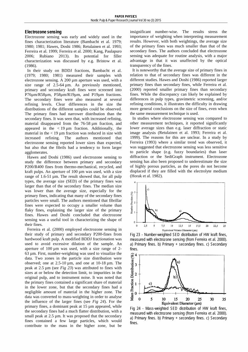
PAPER PHYSICS Nordic Pulp & Paper Research Journal Vol 30 no (3) 2015
Electrozone sensing Electrozone sensing was early and widely used in the fines characterization literature (Bambacht et al. 1979; 1980; 1981; Hawes, Doshi 1986; Retulainen et al. 1993; Ferreira et al. 1999; Ferreira et al. 2000; Kang, Paulapuro 2006; Rubiano 2013). Its potential for filler characterization was discussed by e.g. Bristow et al. (1986).
In their study on BDDJ fractions, Bambacht et al. (1979; 1980; 1981) measured their samples with electrozone sensing. A 200 µm aperture was used, with a size range of 2.5-64 µm. As previously mentioned, primary and secondary kraft fines were screened into P76µm/R58µm, P58µm/R19µm, and P19µm fractions. The secondary fines were also measured at several refining levels. Clear differences in the size the distributions of the different samples could be observed. The primary fines had narrower distribution than the secondary fines. It was seen that, with increased refining, material disappeared from the 76-58 µm fraction, and appeared in the < 19 µm fraction. Additionally, the material in the < 19 µm fraction was reduced in size with increased refining. The authors mentioned that electrozone sensing reported lower sizes than expected, but also that the fibrils had a tendency to form larger agglomerates.
Hawes and Doshi (1986) used electrozone sensing to study the difference between primary and secondary P200/R400 fines from thermo-mechanical, recycled, and kraft pulps. An aperture of 100 µm was used, with a size range of 1.6-51 µm. The result showed that, for all pulp types, the average size (SED) of the primary fines was larger than that of the secondary fines. The median size was lower than the average size, especially for the primary fines, indicating that many of the secondary fines particles were small. The authors mentioned that fibrillar fines were expected to occupy a smaller volume than flaky fines, explaining the larger size of the primary fines. Hawes and Doshi concluded that electrozone sensing was a useful tool in characterizing the shape of their fines.
Ferreira et al. (2000) employed electrozone sensing in their study of primary and secondary P200-fines from hardwood kraft pulp. A modified BDDJ fractionation was used to avoid excessive dilution of the sample. An aperture of 100 µm was used, with a size range of 2-63 µm. First, number-weighting was used to visualize the data. Two zones in the particle size distribution were observed; one at 2.5-10 µm, and one at 10-18 µm. The peak at 2.5 µm (see Fig 23) was attributed to fines with sizes at or below the detection limit, to impurities in the original pulp, and to instrument noise. It was noted that the primary fines contained a significant share of material in the lower zone, but that the secondary fines had a negligible amount of material in the higher zone. The data was converted to mass-weighting in order to analyse the influence of the larger fines (see Fig 24). For the primary fines, a dominant peak at 15 µm appeared, while the secondary fines had a much flatter distribution, with a small peak at 2.5 µm. It was proposed that the secondary fines contained a few large particles, which would contribute to the mass in the higher zone, but be
insignificant number-wise. The results stress the importance of weighting when interpreting measurement results. However, with both weightings, the average size of the primary fines was much smaller than that of the secondary fines. The authors concluded that electrozone sensing was adequate for routine analysis, with a major advantage in that it was unaffected by the optical transparency of the fines.
It is noteworthy that the average size of primary fines in relation to that of secondary fines was different in the different studies. Hawes and Doshi (1986) reported larger primary fines than secondary fines, while Ferreira et al. (2000) reported smaller primary fines than secondary fines. While the discrepancy can likely be explained by differences in pulp types, gravimetric screening, and/or refining conditions, it illustrates the difficulty in drawing more general conclusions on the size of fines, even when the same measurement technique is used.
In studies where electrozone sensing was compared to other measurement techniques, it reported significantly lower average sizes than e.g. laser diffraction or static image analysis (Retulainen et al. 1993; Ferreira et al. 1999). The reasons for this are unclear. In a study by Ferreira (1993) where a similar trend was observed, it was suggested that electrozone sensing was less sensitive to particle shape (e.g. fuzzy boundaries) than laser diffraction or the SediGraph instrument. Electrozone sensing has also been proposed to underestimate the size of highly porous particles, as the pores do not become displaced if they are filled with the electrolyte medium (Horak et al. 1982).
Fig 23 - Number-weighted SED distribution of HW kraft fines, measured with electrozone sensing (from Ferreira et al. 2000). a) Primary fines. b) Primary + secondary fines. c) Secondary fines.
Fig 24 - Mass-weighted SED distribution of HW kraft fines, measured with electrozone sensing (from Ferreira et al. 2000). a) Primary fines. b) Primary + secondary fines. c) Secondary fines.
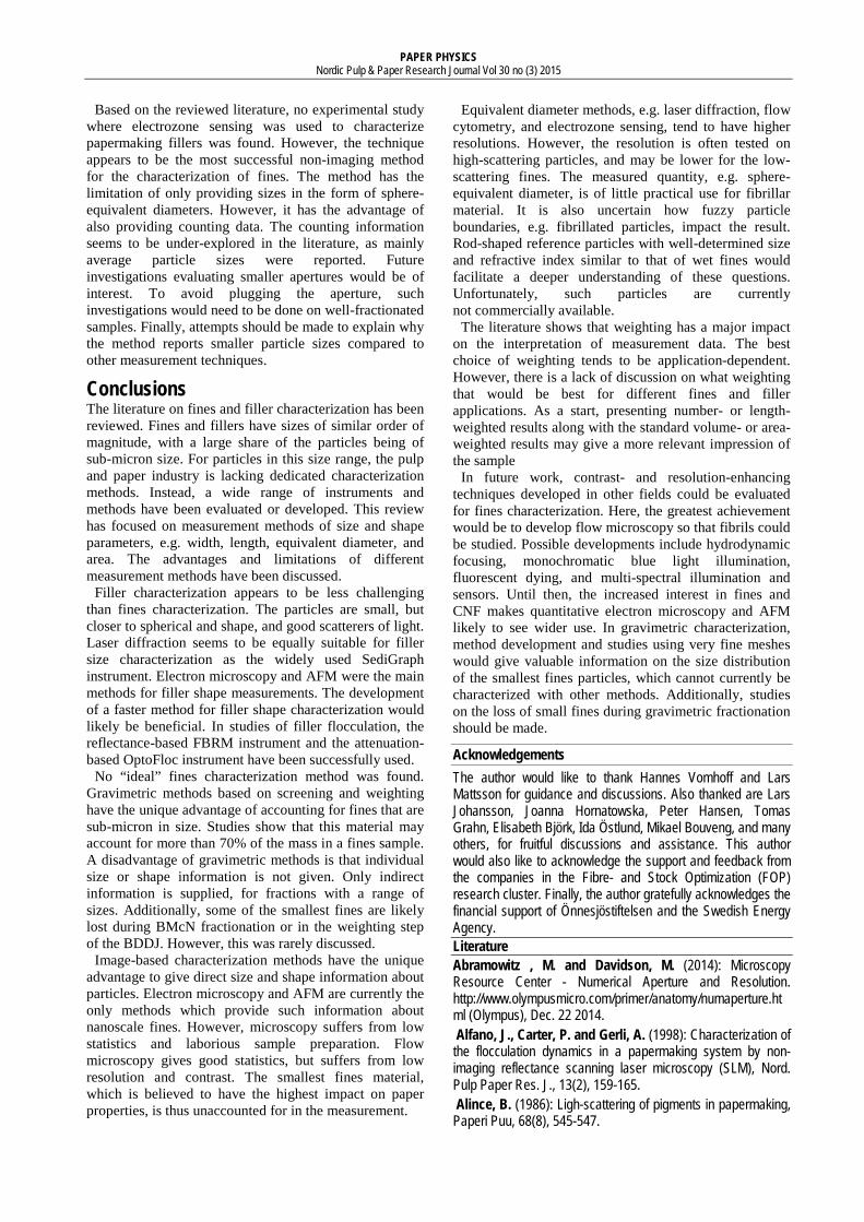
PAPER PHYSICS Nordic Pulp & Paper Research Journal Vol 30 no (3) 2015
Based on the reviewed literature, no experimental study where electrozone sensing was used to characterize papermaking fillers was found. However, the technique appears to be the most successful non-imaging method for the characterization of fines. The method has the limitation of only providing sizes in the form of sphere-equivalent diameters. However, it has the advantage of also providing counting data. The counting information seems to be under-explored in the literature, as mainly average particle sizes were reported. Future investigations evaluating smaller apertures would be of interest. To avoid plugging the aperture, such investigations would need to be done on well-fractionated samples. Finally, attempts should be made to explain why the method reports smaller particle sizes compared to other measurement techniques.
Conclusions The literature on fines and filler characterization has been reviewed. Fines and fillers have sizes of similar order of magnitude, with a large share of the particles being of sub-micron size. For particles in this size range, the pulp and paper industry is lacking dedicated characterization methods. Instead, a wide range of instruments and methods have been evaluated or developed. This review has focused on measurement methods of size and shape parameters, e.g. width, length, equivalent diameter, and area. The advantages and limitations of different measurement methods have been discussed.
Filler characterization appears to be less challenging than fines characterization. The particles are small, but closer to spherical and shape, and good scatterers of light. Laser diffraction seems to be equally suitable for filler size characterization as the widely used SediGraph instrument. Electron microscopy and AFM were the main methods for filler shape measurements. The development of a faster method for filler shape characterization would likely be beneficial. In studies of filler flocculation, the reflectance-based FBRM instrument and the attenuation-based OptoFloc instrument have been successfully used.
No “ideal” fines characterization method was found. Gravimetric methods based on screening and weighting have the unique advantage of accounting for fines that are sub-micron in size. Studies show that this material may account for more than 70% of the mass in a fines sample. A disadvantage of gravimetric methods is that individual size or shape information is not given. Only indirect information is supplied, for fractions with a range of sizes. Additionally, some of the smallest fines are likely lost during BMcN fractionation or in the weighting step of the BDDJ. However, this was rarely discussed.
Image-based characterization methods have the unique advantage to give direct size and shape information about particles. Electron microscopy and AFM are currently the only methods which provide such information about nanoscale fines. However, microscopy suffers from low statistics and laborious sample preparation. Flow microscopy gives good statistics, but suffers from low resolution and contrast. The smallest fines material, which is believed to have the highest impact on paper properties, is thus unaccounted for in the measurement.
Equivalent diameter methods, e.g. laser diffraction, flow cytometry, and electrozone sensing, tend to have higher resolutions. However, the resolution is often tested on high-scattering particles, and may be lower for the low-scattering fines. The measured quantity, e.g. sphere-equivalent diameter, is of little practical use for fibrillar material. It is also uncertain how fuzzy particle boundaries, e.g. fibrillated particles, impact the result. Rod-shaped reference particles with well-determined size and refractive index similar to that of wet fines would facilitate a deeper understanding of these questions. Unfortunately, such particles are currently not commercially available.
The literature shows that weighting has a major impact on the interpretation of measurement data. The best choice of weighting tends to be application-dependent. However, there is a lack of discussion on what weighting that would be best for different fines and filler applications. As a start, presenting number- or length-weighted results along with the standard volume- or area-weighted results may give a more relevant impression of the sample
In future work, contrast- and resolution-enhancing techniques developed in other fields could be evaluated for fines characterization. Here, the greatest achievement would be to develop flow microscopy so that fibrils could be studied. Possible developments include hydrodynamic focusing, monochromatic blue light illumination, fluorescent dying, and multi-spectral illumination and sensors. Until then, the increased interest in fines and CNF makes quantitative electron microscopy and AFM likely to see wider use. In gravimetric characterization, method development and studies using very fine meshes would give valuable information on the size distribution of the smallest fines particles, which cannot currently be characterized with other methods. Additionally, studies on the loss of small fines during gravimetric fractionation should be made.
Acknowledgements The author would like to thank Hannes Vomhoff and Lars Mattsson for guidance and discussions. Also thanked are Lars Johansson, Joanna Hornatowska, Peter Hansen, Tomas Grahn, Elisabeth Björk, Ida Östlund, Mikael Bouveng, and many others, for fruitful discussions and assistance. This author would also like to acknowledge the support and feedback from the companies in the Fibre- and Stock Optimization (FOP) research cluster. Finally, the author gratefully acknowledges the financial support of Önnesjöstiftelsen and the Swedish Energy Agency. Literature Abramowitz , M. and Davidson, M. (2014): Microscopy Resource Center - Numerical Aperture and Resolution. http://www.olympusmicro.com/primer/anatomy/numaperture.html (Olympus), Dec. 22 2014. Alfano, J., Carter, P. and Gerli, A. (1998): Characterization of the flocculation dynamics in a papermaking system by non-imaging reflectance scanning laser microscopy (SLM), Nord. Pulp Paper Res. J., 13(2), 159-165. Alince, B. (1986): Ligh-scattering of pigments in papermaking, Paperi Puu, 68(8), 545-547.

PAPER PHYSICS Nordic Pulp & Paper Research Journal Vol 30 no (3) 2015
Amnis (2012): ImageStream X Mark II Brochure, Amnis Seattle (WA). Anderson, W., Kozak, D., Coleman, V., Jämting, Å. and Trau, M. (2013): A comparative study of submicron particle sizing platforms: Accuracy, precision and resolution analysis of polydisperse particle size distributions, J. Colloid Interface Sci., 405, 322-330. Athley, K., Granlöf, L., Söderberg, D., Ankerfors, M. and Ström, G. (2012): Mechanical retention: influence of filler floc size and grammage of the fibre web, Nord. Pulp Paper Res. J., 27(2), 202-207. Bambacht, J. P., Hsu, T. H. and Unbehend, J. E. (1981): Analysis of Fines Fractions and Their Influence on Sheet Properties, Report, Empire State Research Institute (ESPRI), Syracuse (NY). Bambacht, J. P. and Unbehend, J. E. (1980): Physical and Chemical Analysis of Classified Pulp Fines Report, Empire State Research Institute (ESPRI), Syracuse (NY). Bambacht, J. P., Unbehend, J. E. and O'Brian, H. E. (1979): Characterization of Primary and Secondary Pulp Fines Report, Empire State Research Institute (ESPRI), Syracuse (NY). Baosupee, D., Massey, A., Nazhad, M. and Hubbe, M. (2014): Heteroagglomeration as a mechanism of retainint CaCO3 particles on the fibrils of cellulosic fines: A study by laser ligth diffraction and microscopy, Colloids Surf., 441, 7. Beckman Coulter (2014a): The Coulter Principle. Acessed Dec. 30 2014a from https://www.beckmancoulter.com/wsrportal/wsr/industrial/particle-technologies/coulter-principle/index.htm (Beckman Coulter ),. Beckman Coulter (2014b): Multisizer 4e Coulter Counter Brochure, Beckman Coulter, Malvern (UK). Bichard, W. and Scudamore, P. (1988): An evaluation of the comparative performance of the Kajaani FS-100 and FS-200 fibre length analyzers, Tappi J., 72(12), 149-155. Biosciences, B. (2000): Introduction to Flow Cytometry: A Learning Guide, BD Biosciences, San Jose (CA). Björk, E., Athley, K. and Thomsson, L. (2012): Advanced techniques to study filler flocs in high shear environments, International Paper Physics Conference, Stockholm (SE), pp. 17-20. Blechschmidt, J., Mallon, U. and Schramm, S. (2000): Quantitative Assessment of Fines in Paper Manufacturing, Wochenblatt für Papierfrabrikation, 5, 300-305. Bohren, C. F. and Huffman, D. R. (2004): Absorption and Scattering of Light by Small Particles, Wiley-VCH Weinheim (DE). Brecht, W. and Holl, M. (1939): Schaffung eines Normalverfahrens zur Gutebewertung von Holzschliffen, Der Papier-fabrikant 10(24), 74-86. Bristow, A., Fineman, I., Lindström, T., Pauler, N., Ulmgren, P., Wågberg, L. and Ölander, K. (1986): Fyllmedel i tryckpapper - Slutrapport, STFI-meddelande, C-131, STFI, Stockholm. Chen, H., Park, A., Heitmann, J. and Hubbe, M. (2009): Importenace of Cellulosic Fines Relative to the Dewatering Rates of Fiber Suspensions, Ind. Eng. Chem. Res., 48, 9106-9112. Chinga-Carrasco, G. (2011): Cellulose fibres, nanofibrils and microfibrils: The morphological sequence of MFC components
from a plant physiology and fibre technology point of view, Nanoscale Res Lett., 6(1), 417-424. Donner Technologies (2014): Further recent history of DIPA 2000. Acessed from http://www.donner-tech.com/page17.html (Donner Technologies), Dec. 29 2014. Eurocon (2014): Pulp on Target, SCOPE, Luleå (SE), pp. 1-26. Ferreira, P., Martins, A. and Figueiredo, M. (2000): Primary and secondary fines from Eucalyptus globulus kraft pulps. Characterization and influence, Paperi Puu, 82(6), 403-408. Ferreira, P., Matos, S. and Figueiredo, M. (1999): Size Characterization of Fibres and Fines in Hardwood Kraft Pulps, Part. Part. Syst. Charact., 16, 20-24. Fineman, I., Bergenblad, H., Pauler, N. and Bouvent, M. (1987): Utvärdering av fällda och malda kalciumkarbonat som fyllmedel i finpapper, STFI-meddelande, D-283, STFI, Stockholm. Fluid Imaging (2014): FlowCAM - Industrial Applications Overview Brochure, Fluid Imaging Technologies Fraschini, C., Chauve, G., Le Berre, J.-F., Ellis, S., Méthot, M., O’Connor, B. and Bouchard, J. (2014): Critical discussion of light scattering and microscopy techniques for CNC particle sizing, Nord. Pulp Paper Res. J., 29(1), 31. Fuente, E., Blanco, A., Negro, C., San Pio, I. and Tijero, J. (2003): Monitoring Flocculation of Fillers in Papermaking, Paper Technology, 44(8), 41-50. GE Healthcare (2014): Typical Properties of Filter Papers and Glass Fiber Filters. Acessed July 21 2014from http://www.gelifesciences.com/webapp/wcs/stores/servlet/catalog/sv/GELifeSciences-se/applications/typical-properties-of-filter-papers-and-glass-fiber-filters (GE Healthcare),. Gélinas, V. and Vidal, D. (2008): Determination of particle shape distribution of clay using an automated AFM image analysis method, TAPPI Advanced Coating Fundamentals Symposium, Montreal (CA), pp. 6-19. Gerli, A., Keiser, B. and Surya, P. (2000): The use of focussed beam reflectance measurement (FBRM) in the development of a new nanosize particle, Appita 54th annual conference, Melbourne (AU), pp. 203-208. Goldszer, K. and Wahlström, T. (2011): Characterization of fines with use of flow cytometry, IMPC International Mechanical Pulping Conference 2011, Xi'an (CN), pp. 58-61. Gooding, R. and Olson, J. (2001): Fractionation in a Bauer-McNett Classifier, J. Pulp Pap. Sci, 27(12), 423-428. Grahn, T. and Björk, E. (2013): Fibre, pulp and stock characterisation - Survey and comparative study, Innventia Report, Innventia AB, Stockholm. Gregory, J. (2005): Particles in Water: Properties and Processes, CRC Press, Boca Raton (FL). Guay, D., Sutherland, N., Rantanen, W., Malandri, N., Stephens, A., Mattingly, K. and Schneider, M. (2005): Comparison of Fiber Length Analyzers, TAPPI Practical Papermaking Conference 2005, Milwaukee (WI) Haapala, A., Laitinen, O., Karinkanta, P., Miilatainen, H. and Niinimäki, J. (2013): Optical characterization of micro-scale cellulose particles and wood powder, Appita Annual Conference 2013, Melbourne (AU), pp. 70-77. Hak-Lae, L., Hye-Jung, Y. and Kyong-Ho, L. (2006): Effects of the size distribution of preflocculated GCC on the physical properties of paper, 3rd International Symposium on Emerging
PAPER PHYSICS Nordic Pulp & Paper Research Journal Vol 30 no (3) 2015
Technologies of Pulping and Papermaking. Research progress in pulping and papermaking., Guangzhou (CN), pp. 472-477. Hawes, J. and Doshi, M. (1986): The contribution of different types of fines to the properties of handsheets made from recycled paper, IPC Technical Paper Series, 178, Institute of Paper Chemistry, Appleton. Heikkurinen, A. and Hattula, T. (1993): Mechanical Pulp Fines - Characterization and Implications for Defibration Mechanisms, 18:th International Mechanical Pulping Conference Oslo (NO), pp. 269-307. Hirn, U. and Bauer, W. (2006): A review of image analysis based methods to evaluate fiber properties, Lenzinger Berichte, 86, 96-103. Hirsch, G. (2012): Altpapierfeinstoffe – Trennbarkeit und Festigkeitspotenzial, Thesis from Technischen Universität Darmstadt, Darmstadt. Hitachi (2011): Ultra-high Resolution Scanning Electron Microscope SU9000. Acessed Dec. 22 2011 from http://www.hitachi-hitec.com/global/em/fe/su9000.html (Hitachi High-Tech),. Holm, M. and Manner, H. (2001): Increasing filler content of fine paper by using preflocculation, Mednarodni Letni Simpozij International Symposium, Bled (SI), pp. 167-170. Holm, M. and Manner, H. (2003): Stability of preflocculated calcium carbonate filler flocs, 57th Appita Annual Conference, Melbourne (AUS), pp. 337-342. Horak, D., Peska, J., Svec, F. and Stamberg, J. (1982): The Influence of Porosity of Discrete Particles upon their Apparent Dimensions as Measured by the Coulter Principle, Powder Technology, 31, 263-267. Horiba (2012): A Guidebook to Particle Size Analysis, Horiba Scientific, Irvine (CA). Hornatowska, J. and Björk, E. (2007): Selective staining of fibres - A literature review and experimental trials, STFI-Packforsk report, IR 56, STFI-Packforsk, Stockholm. ISO 9276-1 standard: Representation of results of particle size analysis - Part 1: Graphical representation, International Organization for Standardization (ISO), 1998. ISO 13317-3 standard: Determination of particle size distribution by gravitational liquid sedimentation methods - Part 3: X-ray gravitational technique, International Organization of Standardization (ISO), 2001. ISO 13322-2 standard: Particle size analysis - Image analysis methods - Part 2: Dynamic image analysis methods, International Organization for Standardization (ISO), 2006. ISO 9276-6 standard: Representation of results of particle size analysis - Part 6: Descriptive and quantitative representation of particle shape and morphology, International Organization of Standardization (ISO), 2008. ISO 13322-1 standard: Particle size analysis - Image analysis methods - Part 1: Static image analysis methods, International Organization for Standardization (ISO), 2014a. ISO 9276-2 standard: Representation of results of particle size analysis - Part 2: Calculation of average particle sizes/diameters and moments from particle size distributions, International Organization for Standardization (ISO), 2014b. Izon Science (2014): qNano instrument description. Acessed Nov 25 2014 from http://www.izon.com/products/qnano/qnano/ (Izon Science),.
Jap, T. (1997): Möglichkeit und Grenzen der Feinstoffpartikelmessung mit einem neuen Partikelmessgerät, Thesis from Technische Universitet Darmstadt, Darmstadt. Jasco (2013): Wet-dispersion type Particle Image Analyzers Brochure, Jasco International Easton (MD). Kang, T. and Paulapuro, H. (2006): Characterization of chemical pulp fines, Tappi J. , 5(2), 25-28. Kangas, H. (2007): Surface chemical and morphological properties of mechanical pulps, fibres and fines, Thesis from Helsinki University of Technology, Espoo. Kangas, H. and Kleen, M. (2004): Surface chemical and morphological properties of mechanical pulp fines, Nord. Pulp Paper Res. J., 19(2), 191-199. Karlsson, H. and Pettersson, J. (1985): Method of measuring fines in pulp suspensions, US Patent 4.514.257, Issued Apr. 30, 1985. Kaunonen, A. and Luukkonen, M. (1992): Practical experiences using continuous freeness measurement, Tappi J, 75(3), 159-164. Krogerus, B., Eriksson, L., Sundberg, A., Mosbye, J., Ahlroth, A., Östlund, I. and Sjöström, L. (2002a): Fines in closed circuits - Final report, SCAN Forsk report, 740, KCL Krogerus, B., Fagerholm, K. and Tiikkaja, E. (2002b): Fines from different pulps compared by image analysis, Nord. Pulp Paper Res. J., 17(4), 440-444. Kumar, S., Julien-Saint-Amand, F., Passas, R., Fabry, B. and Scheler, M. (2010): Lab scale fine-fractionation of deinked pulp and particle microscopic analysis, XXI TECNICELPA Conference and Exhibition / VI CIADICYP 2010, Lisbon (PT), pp. 1-6. Laitinen, O. K., Kalle, Stoor, T. and Niinimäki, J. (2011): Fractionation of pulp and paper particles selectively by size, BioResources, 6(1), 672-685. Lhotta, T., Villforth, K. and S, S. (2007): Fibre Classification - Advanced Fibre Analysis for Quality Control and Process Optimisation in Stock Preparation, Das Papier, 25, 50-53. Li, L., Collis, A. and Pelton, R. (2002): A New Analysis of Filler Effects on Paper Strength, J. Pulp Pap. Sci, 28(8), 267-273. Lidbrant, O. M., U.-B. (1980): Changes in fiber sctructure due to refining as revealed by SEM, International symposium on fundamental concepts of refining, Appleton (WI), pp. 61-74. LUT (2012): Colloids in Papermaking, Lappeenranta University of Technology (LUT), Lappeenranta. Luukko, K. (1999): Fines quantity and quality in controlling pulp and paper quality, International Mechanical Pulping Conference IMPC99, Houston (TX), pp. 1-9. Luukko, K., Kemppainen-Kajola, P. and Paulapuro, H. (1997): Characterization of mechanical pulp fines by image analysis, Appita J., 50(5), 387-391. Luukko, K. and Paulapuro, H. (1999): Mechanical pulp fines: Effect of particle size and shape, Tappi J., 82(2), 95-100. Maloney, T. C., Ataide, J., Kekkonen, J., Fordsmand, H. and Hoeg-Petersen, H. (2005): Changes to PCC structure in papermaking, XIX National Technicelpa Conference, Lisbon (PT), pp. 1-7. Malvern Instruments (2010): Mie theory - the first 100 years, Inform White Paper, Malvern Instruments, Malvern (UK).
PAPER PHYSICS Nordic Pulp & Paper Research Journal Vol 30 no (3) 2015
Malvern Instruments (2011): Mastersizer 3000 brochure, Malvern Instruments, Malvern (UK). Malvern Instruments (2012): A basic guide to particle characterization, Inform White Paper, Malvern Instruments, Malvern (UK). Marton, R. and Robie, J. (1969): Characterization of Mechanical Pulps By a Settling Technique, Tappi J., 52(12), 2400-2406. Merkus, H. (2009): Overview of Size Characterization Techniques, In in Particle Size Measurements, Springer, Netherlands. pp. 137-194. Metso, A. (2006): KajaaniFiberLab(TM) brochure, Metso Automation Mettler Toledo (2014): ParticleTrack With FBRM Technology. Acessed Dec. 30 2014 from Mettler Toledo http://us.mt.com/us/en/home/products/L1_AutochemProducts/FBRM-PVM-Particle-System-Characterization/FBRM.html,. Micrometics (2014): SediGraph Method Overview. Acessed Jan 21 2014 from http://www.micromeritics.com/Product-Showcase/SediGraph-III-Plus/SediGraph-Method-Overview.aspx. Microtrac (2014): Bluewave/S3500 SIA Brochure, Micrtotrac Europe GmbH, Meerbusch (DE). Mosbye, J. (1999): Fractionation and chemical analysis of fines, 27:th EUCEPA conference, Grenoble (FR), pp. 317-321. Munktell (2014): Filtration and Separation Technology Brochure, Ahlstrom Munktell, Falun (SE). Mörseburg, K. (1999): Development and Characterization of Norway Spruce Pressure Groundwood Pulp Fibres, Thesis from Åbo Akademi, Åbo, Finland. NanoSight (2013): Nanoparticle Tracking Analysis (NTA). Acessed Mar. 17 2013 from Malvern Instruments, http://www.nanosight.com/technology/nanoparticle-tracking-analysis-nta. Okamoto, T. and Meshitsuka, G. (2010): The nanostructure of kraft pulp 1: evaluation of various mild drying methods using field emission scanning electron microscopy, Cellulose, 17(6), 1171-1182. Olofsson, K. (1997): Mätmetod för fibrers fibrilleringsgrad, STFI-Rapport, TF 56, STFI, Stockholm (SE). Paavilainen, L. (1990): Importance of particle size - fibre length and fines - for the characterization of softwood kraft pulp, Paperi Puu, 72(5), 516-526. Pabst, W. and Gregorova, E. (2007): Characterization of particles and particle systems. Acessed from http://www.vscht.cz/sil/keramika/Characterization_of_particles/CPPS%20_English%20version_.pdf (Institute of Chemical Technology (ICT)), 2007. Paiva, A. T., Sequeira, S. M., Evtuguin, D. V., Kholkin, A. L. and Portugal, I. (2007): Nanoscale Structure of Cellulosic Materials: Challenges and Opportunities for AFM, In in Modern Research and Educational Topics in Microscopy, Formatex. pp. 726-733. Pelton, R., Jordan, B. and Allen, L. (1985): Particle size distributions of fines in mechanical pulps and some aspects of their retention in papermaking, Tappi J, 86(2), 91-94.
Pettersson, T. (2010): On-line crill measurements for improved control of refining, Control Systems, Stockholm (SE), pp. 1-7. ProteinSimple (2015): MFI™ Technology. Acessed Jun. 25 2015 from http://www.proteinsimple.com/mfi_technology.html (ProteinSimple). QAQC Lab (2014): Sieve conversion chart. Acessed Dec. 30 2014 from QAQC Lab http://www.qclabequipment.com/SIEVE_CONVERSION_CHART.pdf. Rawle, A. (1993): Basic Principles of Particle Size Analysis. Acessed from (Malvern Instruments), 1993. Retulainen, E., Luukko, K., Nieminen, K., Pere, J., Laine, J. and Paulapuro, H. (2001): Papermaking quality of fines from different pulps - The effect of size, shape and chemical composition, 55:th Appita Annual Conference, Hobart (AU), pp. 209-314. Retulainen, E., Moss, P. and Nieminen, K. (1993): Effect of fines on the properties of fibre networks, 10th Fundamental Research Symposium, Oxford (EN), pp. 727-769. Richardson, D. and Grubb, M. (2013): Evaluation of mineral filler's interaction with wood extractive colloids in pulp & paper mill process waters using flow cytometry, 17th International Symposium on Wood, Fibre and Pulping Chemistry (ISWFPC), Vancouver (CA), pp. 2317-2324. Rissanen, R., Leionen, A., Haapapa, A. and Kyyrönen, P. (2011): Comparison of sample pre-treatment methods on flow cytometry measurement of mechanical pulp, TAPPI Peers 2011, Portland (OR), pp. 141-146. Rodrigues Alves, C. (2011): Method development for analysis of Ray cells content in Thermomechanical Pulp of Spruce, Thesis from University of Porto Rubiano, J. E. B. (2013): Characterization of a pulp fractionation process for paper and board production, Innventia Report, Innventia, Stockholm. Rundlöf, M. (2002): Interaction of dissolved and colloidal substances with fines of mechanical pulp - Influence on sheet properties and basic aspects of adhesion, Thesis from KTH Royal Institute of Technology, Stockholm. Rundlöf, M., Htun, M. and Wågberg, L. (2000): The Importance of the Experimental Method When Evaluating the Quality of Fines of Mechanical Pulps, J. Pulp Pap. Sci, 26(9), 301-305. Rydefalk, S. (2009): Particle Measurement Using Fluctuations in the Regular Transmittance of Light Through a Particle Dispersion, Thesis from KTH Royal Institute of Technology, Stockholm. Rådberg, W. (2010): Determination of Distribution of Fines in a Paper Structure using Fluorescence Microscopy - an introduction, Thesis from University of Karlstad, Karlstad. SCAN-CM 6:05 standard: Fibre fractionation in the McNett classifier, SCAN-test, 2005. Seth, R. S. (2003): The measurement and significance of fines, Pulp Paper Can., 104(2), 41-44. Shimizu, H., Usuda, M. and Kadoya, T. (1981a): Evaluation of Fibrillation of Paper Making Fibers in Suspension by Optical Method - Part II, Japan Tappi, 35(10), 913-920.
Shimizu, H., Usuda, M. and Kadoya, T. (1981b): Evaluations of Fibrillation of Paper Making Fibres in Suspension by Optical Method - Part I, Japan Tappi, 35(7), 609-615.
Steenberg, B., Sandgren, B. and Wahren, D. (1960): Studies on Pulp Crill, Svensk Papperstidning, 63(12), 395-397.
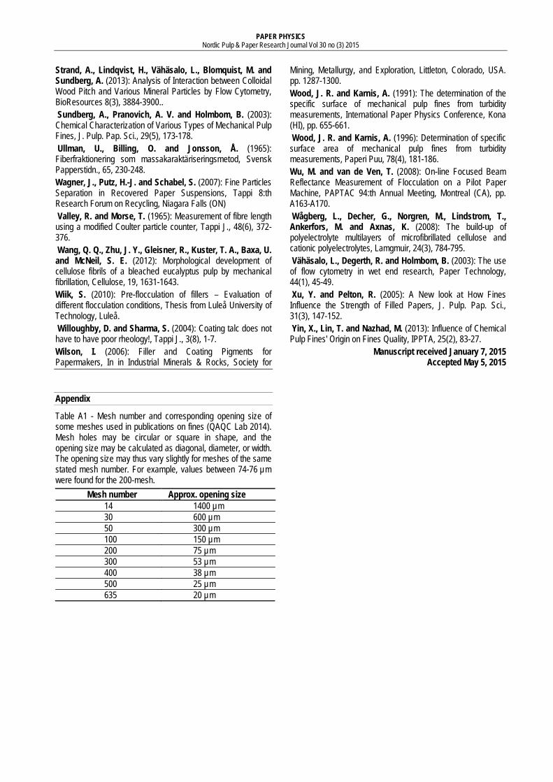
PAPER PHYSICS Nordic Pulp & Paper Research Journal Vol 30 no (3) 2015
Strand, A., Lindqvist, H., Vähäsalo, L., Blomquist, M. and Sundberg, A. (2013): Analysis of Interaction between Colloidal Wood Pitch and Various Mineral Particles by Flow Cytometry, BioResources 8(3), 3884-3900.. Sundberg, A., Pranovich, A. V. and Holmbom, B. (2003): Chemical Characterization of Various Types of Mechanical Pulp Fines, J. Pulp. Pap. Sci., 29(5), 173-178. Ullman, U., Billing, O. and Jonsson, Å. (1965): Fiberfraktionering som massakaraktäriseringsmetod, Svensk Papperstidn., 65, 230-248. Wagner, J., Putz, H.-J. and Schabel, S. (2007): Fine Particles Separation in Recovered Paper Suspensions, Tappi 8:th Research Forum on Recycling, Niagara Falls (ON) Valley, R. and Morse, T. (1965): Measurement of fibre length using a modified Coulter particle counter, Tappi J., 48(6), 372-376. Wang, Q. Q., Zhu, J. Y., Gleisner, R., Kuster, T. A., Baxa, U. and McNeil, S. E. (2012): Morphological development of cellulose fibrils of a bleached eucalyptus pulp by mechanical fibrillation, Cellulose, 19, 1631-1643. Wiik, S. (2010): Pre-flocculation of fillers – Evaluation of different flocculation conditions, Thesis from Luleå University of Technology, Luleå. Willoughby, D. and Sharma, S. (2004): Coating talc does not have to have poor rheology!, Tappi J., 3(8), 1-7. Wilson, I. (2006): Filler and Coating Pigments for Papermakers, In in Industrial Minerals & Rocks, Society for
Mining, Metallurgy, and Exploration, Littleton, Colorado, USA. pp. 1287-1300. Wood, J. R. and Karnis, A. (1991): The determination of the specific surface of mechanical pulp fines from turbidity measurements, International Paper Physics Conference, Kona (HI), pp. 655-661. Wood, J. R. and Karnis, A. (1996): Determination of specific surface area of mechanical pulp fines from turbidity measurements, Paperi Puu, 78(4), 181-186. Wu, M. and van de Ven, T. (2008): On-line Focused Beam Reflectance Measurement of Flocculation on a Pilot Paper Machine, PAPTAC 94:th Annual Meeting, Montreal (CA), pp. A163-A170. Wågberg, L., Decher, G., Norgren, M., Lindstrom, T., Ankerfors, M. and Axnas, K. (2008): The build-up of polyelectrolyte multilayers of microfibrillated cellulose and cationic polyelectrolytes, Lamgmuir, 24(3), 784-795. Vähäsalo, L., Degerth, R. and Holmbom, B. (2003): The use of flow cytometry in wet end research, Paper Technology, 44(1), 45-49. Xu, Y. and Pelton, R. (2005): A New look at How Fines Influence the Strength of Filled Papers, J. Pulp. Pap. Sci., 31(3), 147-152. Yin, X., Lin, T. and Nazhad, M. (2013): Influence of Chemical Pulp Fines' Origin on Fines Quality, IPPTA, 25(2), 83-27.
Manuscript received January 7, 2015 Accepted May 5, 2015
Appendix
Table A1 - Mesh number and corresponding opening size of some meshes used in publications on fines (QAQC Lab 2014). Mesh holes may be circular or square in shape, and the opening size may be calculated as diagonal, diameter, or width. The opening size may thus vary slightly for meshes of the same stated mesh number. For example, values between 74-76 µm were found for the 200-mesh.
Mesh number Approx. opening size 14 1400 µm 30 600 µm 50 300 µm 100 150 µm 200 75 µm 300 53 µm 400 38 µm 500 25 µm 635 20 µm
Related Documents


