Nonstationary Random Critical Seismic Excitations

NONSTATIONARY RANDOM CRITICAL

SEISMIC EXCITATIONS

By R. N. Iyengar1 and C. S. Manohar2

ABSTRACT: A method is presented to find nonstationary random seismic excitations with a constraint on mean square value such that the response variance of a given linear system is maximized. It is also possible to incorporate the dominant input frequency into the analysis. The excitation is taken to be the product of a deterministic enveloping function and a zero mean Gaussian stationary random process. The power spectral density function of this process is determined such that the response variance is maximized. Numerical results are presented for a single-degree system and an earth embankment modeled as shear beam.

INTRODUCTION

Conventional methods of seismic analysis of structures follow either the smooth design response spectrum method or the time history analysis method. As an alternative the method of critical excitation was proposed by Drenick (4). This method consists of finding the excitation from a class of allowable inputs that produces the highest response in a given system. Such an excitation is termed the critical excitation. Drenick (3,4,5) considered the mean square intensity of excitation as known. After applying Schwarz inequality on Duhamel 's integral solution, he showed that the critical excitation for a given system is its impulse response function reversed in time. Such an excitation had deterministic structure and produced highly conservative results. Shinozuka (12) discussed the same problem with the foreknowledge of the envelope of the modulus of the Fourier transform of excitation in defining an allowable class of inputs . Iyengar (7) included the nonstationary enveloping trend of the seismic excitations into the same approach. Wang, et al. (14), introduced the concept of subcritical excitation, which enhances the practical applicability of the critical excitations further. This excitation was chosen from a set of recorded accelerograms that differ from the critical excitation in a minimum mean square sense. The method has also been extended for the case of multiple constraints, wherein the constraints on peak values of velocity and acceleration are imposed in addition to the intensity constraint (2,6). An assessment of this method as applied to the analysis of nuclear plants and other structures of importance has also been made (1,2).

Recently the present authors (8) have outlined a new approach for arriving at a critical excitation which is stochastic in nature. In this approach, the power spectral density (PSD) function of a stationary input with given variance which maximizes the response variance of a linear

'Prof., Dept. of Civ. Engrg., Indian Inst, of Sci., Bangalore 560 012, India. 2Research Scholar, Dept. of Civ. Engrg., Indian Inst, of Sci., Bangalore, India. Note.—Discussion open until September 1, 1987. To extend the closing date

one month, a written request must be filed with the ASCE Manager of Journals. The manuscript for this paper was submitted for review and possible publication on December 12, 1985. This paper is part of the Journal of Engineering Mechanics, Vol. 113, No. 4, April, 1987. ©ASCE, ISSN 0733-9399/87/0004-0529/$01.00. Paper No. 21406.

529

Downloaded 04 Apr 2009 to 203.200.43.195. Redistribution subject to ASCE license or copyright; see http://pubs.asce.org/copyright

system is determined. In the following, this method is generalized to incorporate the nonstationary nature of seismic excitations. Here the class of allowable inputs is characterized by its given mean square value, duration, and nonstationary trend. A way of controlling the average zero crossing rate and frequency content of the excitation is also indicated. Numerical examples are presented for a single degree of freedom system and for a 33.3-m tall earth dam.

ANALYSIS

The input is modeled as a nonstationary random process

x(t) = v(t)w(t) (1)

where w(t) = a Gaussian stationary random process with zero mean and known variance; and v(t) = a known deterministic enveloping function. Following Shinozuka and Sato (13), v(t) is taken as

v(t) = exp (-at) - exp (-0£) (2)

where a and (3 = parameters controlling the rise and fall and thus the duration of the input. The autocorrelation of the response of a time invariant linear system under the above input is

Jo Jo Ry (* 1 , h) = | | V{l1)v(^)Rw (T2 - Tl)/» (h ~ Tl)/Z (t2 - T2)rfTl dj2 (3)

Since w is a stationary process, its autocorrelation can be expressed as

RW(T) = S(O) cos Il-rdO (4) o

where S(fi) is the PSD function of w. Thus the response variance can be reduced to the form

o\t) = S(0)H(fi,f)dfi (5) o

Here H(il, t) resembles a time-varying frequency response function. The critical excitation xc(t) is defined as that input which maximizes cr2(i) within a suitable class of functions under the constraint

( E = S(£l)<m (6)

Jo

The problem of finding xc(t) thus reduces to finding S such that cr2(t) is maximized. A particular solution is obtained by expanding the real function VS in the series

Vs = X «Mn) • •••'•• (7)

where fa (i = 1, 2, ...) = a known set of orthonormal functions such that

530


fotydO, = 0; iV; ' (8a)

htydSl =1; i=j (86)

After combining Eq. 5 with Eq. 6 through a Lagrangian multiplier, the function to be maximized is

L[«i ,«2, . . . , M<(*)] = (24>,<f>;) H(fi, f)««l - M-(0(2«i -E) (9) Jo

Further, imposing the conditions dL/ddj = 0 (i, = 1, 2, ...) and 8L/d\i = 0 one gets

2«,I ( ,(0-^0«y = 0; (; = 1,2,...) (10)

i«?=E (ID

-i in(t) = htyH(n,t)dn (12) Jo

This is an algebraic eigenvalue problem that can be solved using standard techniques. Thus one can get the eigenvalues |x,(f) (i = 1, 2, . . .) and the corresponding eigenvectors {a\i,a2i,...) with the normalization condition of Eq. 11. Further, substitution of Eq. 10 in Eq. 5 leads to

(T2(0 = \L(t)E (13)

This shows that while it is possible to get as many solutions as the number of terms in the expansion for the PSD function, it is the largest eigenvalue and the corresponding eigenvector that lead to the highest response variance. This is true for every time instant t. For finding the critical excitation in a given interval of time, the above exercise has to be repeated for every t. The excitation leading to the maximum response is taken as the desired solution.

ORTHONORMAL FUNCTIONS

The first step in the application of the method just detailed is the selection of a suitable set of orthonormal functions <}>, for expanding the PSD function. It is clear that several different sets of functions could be selected for this purpose. Here, for the sake of illustration, two sets of functions as given by Lee (9) have been chosen. The first set consists of linear combinations of exponentials, the first three terms of which are

4»i(0) = V2p exp (-pfl) (14)

<h(n) = 2Vp[2 exp (-pft) - 3 exp (-2pO)] (15)

531


4>3(fl) = V6p[3 exp (-pfl) - 12 exp (-2p(l) + 10 exp (-3pft)] (16)

The second set is made up of the Laguerre polynomials, which are generated using

£*((!) = \flq

..+(-!)*

(2t7)fcnfc fc(2t?)*'"1 n ^ " 1 fc(fe l)(2(?)fc-2fi'c

fc (A: - 1) 2(k - 2)

exp (-tjCl); (k = 0, 1, 2, ...) (17)

Here p and q are parameters that can be effectively used to control the average zero crossing rate N0 or equivalently, the dominant frequency content of the input. Irrespective of the type of function used for the representation, one would expect to arrive at the same result as the number of terms are increased. However, in practice one has to limit the number of terms. This acts as a constraint and thus different sets of basis functions would lead to differing solutions.

SINGLE DEGREE OF FREEDOM (SDOF) SYSTEMS

A linear time invariant system

y + 2-nwy + co2y = v{t)w{t) (18)

is considered. The function H in Eq. 5 for this system is

H(il,t) = »(TI)I>(T2)/Z(£ ~ Ti)fc(* - T2) cos fi(T2 - T1)dT1dT2 (19) Jo Jo

where h(t) = coj1 exp (—ijcot) sin <adt; o),j = co(l - in2)172 (20)

is the impulse response function of the system. Simplifying Eq. 19 one gets

H{£l,i) = sin flTv(i)h(t — j)dj COS iljv(T)h(t ~ T)dT (21)

EXAMPLE

Let it be required to find the critical excitation of ten sec duration, for a set of SDOF systems with t) = 0.05. The parameters of the modulating function v(t) are taken as a = 0.5 and (3 = 1.0 to get the desired non-stationariness and duration. The constraint of Eq. 6 is indirectly prescribed in terms of a desired average root-mean-square (RMS) intensity of the ground acceleration. Here this RMS value of the critical input is taken as O.lg. From Eq. 1 it follows that

i fT i C (x\t))dt = - v2{t)(w\t))dt (22)

and thus E = (w2(t)) = 0.01g2T

(23)

v2{t)dt

532


0.15

.1 0 080 I

0060

0040

0-020

1

1 J 1 1

-1 1 1 1 1

1 % i

A/ //A

i ) / / /

f n » 2 0 Hz fn =6.0 Hz f n = 8 0 Hz

• fn -10.0 Hz

\ )C\ A \ \ / \ * \

/ \ \ Y

60 60 60 100

-rt- rad/sec

(b)

FIG. 1.—Critical Power Spectral Density Functions for SDOF Systems: (a) In Terms of Exponentials; (b) In Terms of Laguerre Polynomials

Critical PSD functions corresponding to the highest eigenvalue of Eq. 10 have been computed using both the exponential functions and the Laguerre polynomials of Eqs. 14-17. In both cases, seven terms are included in the expansion. These PSD functions are presented in Figs. 1(a)

3.2 4.0 48 Time .sec

FIG. 2.—Simulated Sample of Critical Excitation for 3-Hz System, p = 0.008, r\ 0.05

533 Downloaded 04 Apr 2009 to 203.200.43.195. Redistribution subject to ASCE license or copyright; see http://pubs.asce.org/copyright

40

30

sec

^ 20

10

n

7.0 Hz - — 5 - O H z

3-0Hz 1.0Hz

\

i i" T ~~ 0.01 003 005 007 O09

P 0-01 0-03 O05 0-07

1 (»

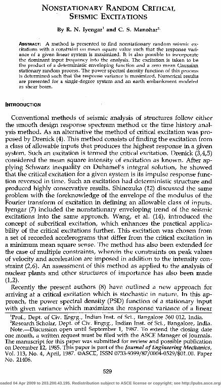
FIG. 3.—Average Zero Crossing Rate: (a) Function of p; (b) Function of i

and 1(b) for both cases. As may be expected beforehand, the critical PSD functions are narrow-banded, since the systems have a very low value of damping. Also, the PSD functions show dominant peaks at the natural frequency of the considered systems. However, the expected non-stationariness and random nature are reflected in the samples generated

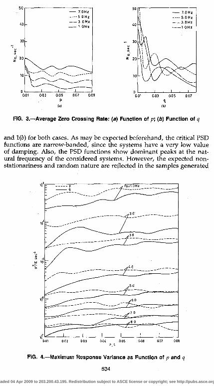
FIG. 4.-—Maximum Response Variance as Function of p and q

534


from these PSD functions. A typical sample of a Gaussian process generated for a 3-Hz system is shown in Fig. 2. It is easy to observe that the parameter p of the exponentials and q of the Laguerre polynomials control the bandwidth of the critical PSD functions. In the above analysis, these are chosen beforehand. Thus the class of admissible functions for VS have also been restricted in terms of the given value of p or q. It is possible to remove this restriction by maximizing the function L of Eq. 9 with respect to these parameters. This would complicate the solution process since the resulting equations become nonlinear. On the other hand, the parameters p and q can be effectively used to reflect the dominant ground or supporting structure frequency in the critical excitation. A measure of this dominant frequency is the average zero crossing rate of the input process. This can be easily found for the critical PSD functions using the well-known Rice's formula (11).

In Fig. 3, the effect of p and q on the average zero crossing rate of the excitation corresponding to the first critical PSD function is shown for SDOF systems. In Fig. 4, the critical response variance as a function of p and q is shown. It may be observed that for the same second moment under the PSD functions, i.e., if not only the variance but also the average zero crossing rates compare, then the representation with either exponentials or Laguerre polynomials lead to the same order of magnitude of response variance.

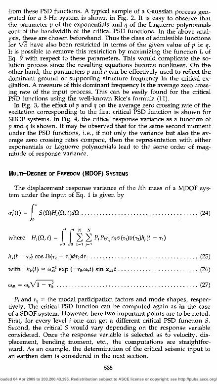
MULTI-DEGREE OF FREEDOM (MDOF) SYSTEMS

The displacement response variance of the ith mass of a MDOF system under the input of Eq. 1 is given by

a?(f) = S(tl)Hi(a,t)dSl (24) Jo

nf N N

X 2 PAwfaM-rdW - TI) k=l ; = 1

hk(t ~ T2) cos {1(T2 - Ji)dT2dTi (25)

with hk(t) =. ujk exp (—i)ka>kt) sin uikt (26)

u* = wtVl - T\1 (27)

Pj and tjj = the modal participation factors and mode shapes, respectively. The critical PSD function can be computed again as in the case of a SDOF system. However, here two important points are to be noted. First, for every level i one can get a different critical PSD function S. Second, the critical S would vary depending on the response variable considered. Once the response variable is selected as to velocity, displacement, bending moment, etc., the computations are straightforward. As an example, the determination of the critical seismic input to an earthen dam is considered in the next section.

535


EARTHEN EMBANKMENT

An earthen dam 33.3 m in height with a triangular cross section (Fig. 5) is considered. It is required to find the critical input such that the lateral displacement variance at the top of the embankment is maximized. The material properties of the dam are taken as shear modulus G = 1.92 X 105 kN/m2; viscous damping coefficient t] = 0.2; and density p = 2.05 x 104 kN/m3. This particular example has been previously considered by Wu (15) in the context of vibration of embankments under seismic load. From the well-known shear beam model, the natural frequencies and eigenfunctions are

'f)(f « 2/o T

»M*) = ZJi(Z„)

(29)

Here J0 and }x are the Bessel's function of the first kind. Z„'s refer to the zeros of Jo . These are Zx = 2.4048; Z2 = 5.5201; Z3 = 8.6537; Z4 = 11.7915; and Z5 = 14.9309. The variance of the top displacement relative to the ground is

(0,f) = S(Q,)H(0,Q,,t)dCl (30)

FIG. 5.—Earthen Dam

TABLE 1.—Critical Input Statistics for Earthen Embankment

Number

0) 1 2 3 4 5 6 7

H,/E (sec4) (2)

0.4042 x 10"3

0.5665 x 10~5

0.2265 x 10"5

0.1453 x 10~5

0.1292 x 10"5

0.1202 x 10~5

0.1345 x 10 6

<r(0,fc) (cm) (3)

8.80 1.04 0.66 0.53 0.50 0.48 0.16

N0 (sec-1) (4)

31.85 7.01 6.65 5.99 2.01

10.66 20.16


40 80 120 160 200

-A. rad/sec

FIG. 6.—Critical Power Spectral Density Functions for Earthen Dam

A^H<i«fMvHw^

0.00 3.00 6-00 9.00 12.00 L5.00 115.00 T l t l f SFC

FIG. 7.—Simulated Sample of Critical Excitation for Earthen Dam, p = 0.032

with H(x,a,t)=\ ^ f i M t j W ^ T ^ ^ i f - T , )

Jo Jo i=l ;=1

hj(t - T2) COS fl(T2 - Ti)dTirfT2 (31)

In the computations the first five modes in the above expression have been retained. The nonstationariness and duration of the input are fixed by selecting the modulating function

(32) v(t) = exp (-0.13f) - exp (-0.450

This reaches its peak value of vm = 0.43 at t,„ = 3.9 sec. Since v(t) reduces to about 90% of v,„ at 25 sec, the duration of the input will be about 30 sec. The average RMS value of the input is required to be O.lg. Hence E is again given by Eq. 23. The critical PSD function has been found in terms of a seven term expansion using exponential functions of Eqs. 14-16 with p - 0.032. The response variance is scanned over the interval

537


0-30 sec to arrive at the highest maximum value. This occurs corresponding to tc = 4 sec. The eigenvalues fji,, the extreme variances, and the average rate of zero crossing N0 for the respective inputs are given in Table 1. The first three critical PSD functions thus obtained are shown in Fig. 6. It is seen that these PSD functions are wide-banded. A sample excitation corresponding to the first PSD function is shown in Fig. 7.

ANALYSIS

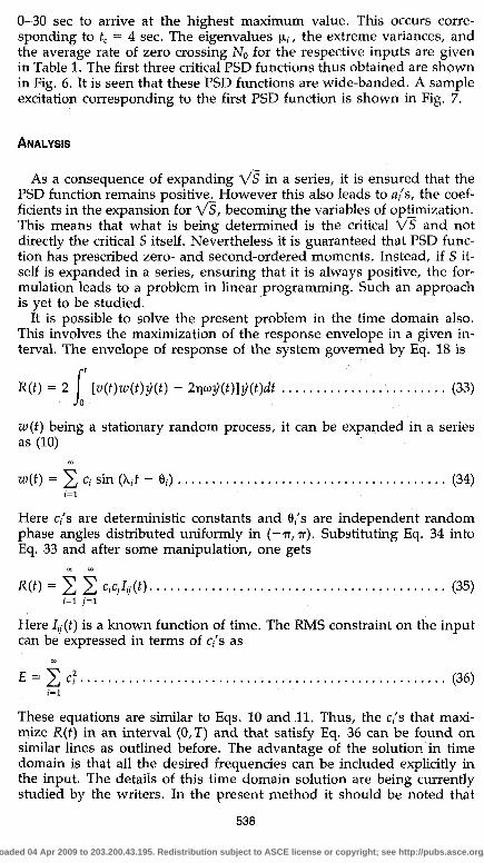
As a consequence of expanding VS in a series, it is ensured that the PSD function remains positive. However this also leads to fl,'s, the coefficients in the expansion for '\fS, becoming the variables of optimization. This means that what is being determined is the critical VS and not directly the critical S itself. Nevertheless it is guaranteed that PSD function has prescribed zero- and second-ordered moments. Instead, if S itself is expanded in a series, ensuring that it is always positive, the formulation leads to a problem in linear programming. Such an approach is yet to be studied.

It is possible to solve the present problem in the time domain also. This involves the maximization of the response envelope in a given interval. The envelope of response of the system governed by Eq. 18 is

R(t) = 2 [v(t)w(t)y{t) - 2^y(t)]y(t)dt (33) Jo

w(t) being a stationary random process, it can be expanded in a series as (10)

w(t) = E ci s i n (X 'f ~ e<) (3 4) i = l

Here c,'s are deterministic constants and 0,'s are independent random phase angles distributed uniformly in (-TT,TT). Substituting Eq. 34 into Eq. 33 and after some manipulation, one gets

*o=i i ww (35) ,'=1 7 = 1

Here 7,;(t) is a known function of time. The RMS constraint on the input can be expressed in terms of c,'s as

E = Ec? (36) f=i

These equations are similar to Eqs. 10 and 11. Thus, the c,'s that maximize R(t) in an interval (0, T) and that satisfy Eq. 36 can be found on similar lines as outlined before. The advantage of the solution in time domain is that all the desired frequencies can be included explicitly in the input. The details of this time domain solution are being currently studied by the writers. In the present method it should be noted that

538


one does not arrive at a unique time history of excitation, but instead an ensemble of time functions forming a stochastic process is obtained.

Critical excitations as developed here are by definition system dependent. Thus at the same site this would lead to different critical inputs for different engineering structures. This naturally is a limitation. To circumvent this difficulty one can find the critical input for the most important structure at a site and use this for the others. A better alternative is to arrive at the critical excitation that is site-dependent, but is independent of the structures to be built. This is similar to the question of fixing-up the worst possible accelerogram for a site with some realistic constraints. With a suitable soil deposit model for the site, the present approach can be used to arrive at the critical input that must be applied at the rock level to maximize the site response at the surface level.

SUMMARY AND CONCLUSIONS

This study outlines a method to arrive at the critical random excitation for a given linear system. For purposes of application in earthquake engineering, the input is taken as an unkown stationary process modulated by a known enveloping function. The mean square value of the random process is assumed to be known. A frequency domain solution is presented for finding the critical power spectral density function of the stationary part of the seismic input. The procedure is illustrated with the example of a single degree of freedom system and that of an earthen embankment. In the former case, it is fairly obvious that the critical power spectral density function should peak near the resonant frequency. However, with heavily damped systems and with multidegree systems, the structure of the input power spectral density function is less obvious. The numerical results obtained show that the sense of criticality is not too severe both in the input and in the response variables. Thus one can expect realistic peak excitation and peak responses from the present solution when used in the seismic analyses of important structures and equipment.

Modification of the method to further restrict the class of allowable inputs and to maximize damage variables other than the response variance is presently under investigation by the writers.

APPENDIX I.—REFERENCES

1. Abdelrahman, A. M., Yun, C. B., and Wang, P. C , "Subcritical Excitation and Dynamic Response of Structures in Frequency Domain," Computers and Structures, Vol. 10, No. 2, Oct., 1978, pp. 761-771.

2. Bedrosian, B., Barbela, M., Drenick, R. F., and Tsirk, A., "Critical Excitation Method for Calculating Earthquake Effects on Nuclear Plant Structures: An Assessment Study," NUREG/CR-1673, RD, U.S. Nuclear Regulatory Commission, Burns and Roe, Inc., Oradell, NJ. , 1980.

3. Drenick, R. F., "Aseismic Design by Way of Critical Excitation," Journal of the Engineering Mechanics Division, ASCE, Vol. 99, No. EM4, Aug., 1973, Proc. Paper 9950, pp. 649-667.

4. Drenick, R. F., "Model-Free Design of Aseismic Structures," Journal of the Engineering Mechanics Division, ASCE, Vol. 96, No. EM4, Aug., 1970, Proc. Paper 7496, pp. 483-493.

539


5. Drenick, R. F., "On a Class of Non-Robust Problems in Stochastic Dynamics," Stochastic Problems in Dynamics, B. L. Clarkson, Ed., Pitman, London, U.K., 1977, pp. 237-255.

6. Drenick, R. F., Novmestky, F., and Bagchi, G., "Critical Excitation of Structures," Wind and Seismic Effects, Proceedings of the 12th Joint UJNR Panel Conference, NBS Special Publication, 1984, pp. 133-142.

7. Iyengar, R. N., "Matched Inputs," Report 47, Series J., Center of Applied Stochastics, Purdue University, West Lafayette, Ind., 1970.

8. Iyengar, R. N., and Manohar, C. S., "System Dependent Critical Stochastic Seismic Excitations," M15/6, Eighth International Conference on SMiRT, Brussels, Belgium, 1985.

9. Lee, Y. W., Statistical Theory of Communications, John Wiley, New York, N.Y., 1960, pp. 459-480.

10. Papoulis, A., Probability, Random Variables, Stochastic Processes, McGraw-Hill, New York, N.Y., 1965.

11. Rice, S. O., "Mathematical Analysis of Random Noise," Selected Papers on Noise and Stochastic Processes, N. Wax, Ed., Dover Publications, Inc., New York, N.Y., 1954, pp. 133-294.

12. Shinozuka, M., 'Maximum Structural Response to Seismic Excitations," Journal of Engineering Mechanics Division, ASCE, Vol. 96, No. EM5, Proc. Paper 7620, Oct., 1970, pp. 729-738.

13. Shinozuka, M., and Sato, Y., "Simulation of Nonstationary Random Processes," Journal of Engineering Mechanics Division, ASCE, Vol. 93, No. EMI, Feb., 1967, pp. 11-40.

14. Wang, P. C , Drenick, R. F., and Wang, W., "Seismic Assessment of High-Rise Buildings," Journal of Engineering Mechanics Division, ASCE, Vol. 104, No. EM2, Proc. Paper 13691, Apr., 1978, pp. 441-456.

15. Wu, T. H., Soil Dynamics, Allyn and Bacon, Inc., Boston, Mass., 1971, pp. 238-241.

APPENDIX II.—NOTATION

The following symbols are used in this paper:

airCi

E fn G 8

H(il,t) h(t),hk(t)

kit) i,j,k

h L

U I

N0

n Pi

P'l Rit)

l\y , l\w

rn S(ft)

= coefficients; = variance of w(t); = system natural frequency in Hz; = shear modulus; = acceleration due to gravity; = frequency response function; = impulse response function; = function of time; = indices; = Bessel's function of first kind nth order; = Lagrangian; = Laguerre polynomial; = height of earth dam; = average rate of zero crossing; = index; = modal participation factor; = parameters in orthonormal expansion; = envelope of response; = autocorrelation functions; = element of modal matrix; = power spectral density function;


T t,h,h

tc t,n

V(t) W(t) x(t). xc(t)

y z„

«,p i i / f\k

e< X M-p

cr2,of T/ Ti , T2

<t>n „̂ n

w,wk

= =: = = = = = = = = = = = = = = = = = = = =

duration of input; time; time to maximum of response variance; time to maximum of v(t); modulating function; Gaussian stationary random process; input random process; critical excitation; displacement of an oscillator; zeros oi }0(x); parameters in v(t); coefficient of viscous damping; phase angles; angular frequency; Lagrangian multiplier; density; variance of response; dummy variables; orthonormal functions; mode shapes; angular frequency; and natural frequency.

541


Nonstationary Random Critical Seismic Excitations

Documents