Nonpoint source pollution and two-part instruments

1 23

Environmental Economics and PolicyStudiesThe Official Journal of the Society forEnvironmental Economics and PolicyStudies / The Official Journal of the EastAsian Association of Environmental andResource Economics ISSN 1432-847XVolume 15Number 3 Environ Econ Policy Stud (2013)15:237-258DOI 10.1007/s10018-012-0052-4

Nonpoint source pollution and two-partinstruments

Renan-Ulrich Goetz & Yolanda Martínez

1 23

Your article is protected by copyright and

all rights are held exclusively by Springer

Japan. This e-offprint is for personal use only

and shall not be self-archived in electronic

repositories. If you wish to self-archive your

article, please use the accepted manuscript

version for posting on your own website. You

may further deposit the accepted manuscript

version in any repository, provided it is only

made publicly available 12 months after

official publication or later and provided

acknowledgement is given to the original

source of publication and a link is inserted

to the published article on Springer's

website. The link must be accompanied by

the following text: "The final publication is

available at link.springer.com”.

RESEARCH ARTICLE

Nonpoint source pollution and two-part instruments

Renan-Ulrich Goetz • Yolanda Martınez

Received: 31 January 2012 / Accepted: 2 October 2012 / Published online: 20 October 2012

� Springer Japan 2012

Abstract As an alternative to the existing environmental policy instruments,

recent literature proposes to combine different policy instruments (two-part

instruments) which have most of the properties of a first-best Pigouvian tax while

minimizing the need for monitoring and enforcement. This article explores the

design and applicability of a policy based on two-part instruments to control non-

point source pollution. Applying this approach, however, leads to a moral hazard

problem, since it is not only the input itself that is responsible for the pollution but

also the way it is applied. The analysis determines the optimal combinations of taxes

and subsidies as a function of the ability to observe the output and the applied

inputs. In an empirical illustration we determine the magnitude of the taxes and

subsidies to establish the socially optimal level of nitrate emissions from livestock

manure for a region in northeast Spain.

Keywords Two-part instruments � Nonpoint pollution � Moral hazard

JEL Classification D62 � Q10 � Q50 � Q53

1 Introduction

Policies makers often face the difficult task to design policies to control

environmental problem which should be effective, efficient, sustainable, politically

feasible, coherent with the existing legal framework and should provide incentive

R.-U. Goetz

Department of Economics, University of Girona, Campus Montilivi, s/n, 17071 Girona, Spain

e-mail: [email protected]

Y. Martınez (&)

Department of Economic Analysis, University of Zaragoza, Gran Via, 2-4, 50004 Zaragoza, Spain

e-mail: [email protected]

123

Environ Econ Policy Stud (2013) 15:237–258

DOI 10.1007/s10018-012-0052-4

Author's personal copy

for innovations. Given the large number of disperse criteria the optimal policy has to

meet; it is not surprising that the economic literature has not been able to provide a

clear ranking of the available policies.

Apart form the inherent properties of the different regulatory approaches the

choice of the correct policy instrument is also determined by the specific

characteristic of each environmental problem. Differences in climatic and geomor-

phologic characteristics make certain locations within a catchment more vulnerable

to nonpoint pollution than others and demands that instruments should be designed

site specific (Panagopoulos et al. 2011). This requirement aggravates the major

obstacle for the regulation of nonpoint pollution that emissions are either not

observable or cannot be observed at a reasonable cost. Therefore, it is impossible to

attribute emissions to particular polluters, and the use of first-best instruments like a

Pigouvian tax on the emissions is infeasible.

Alternatively, economists have focused on designing instruments to control

pollution directly, e.g. economic incentives or standards. However, this requires that

the regulated inputs or management practices can be truncated to a subset of choices

that can be observed easily and is highly correlated with the emissions of the

pollutant (Shortle and Abler 1998; Dosi and Tomasi 1994). This restriction limits

these approaches to being second-best. Moreover, enforcing these approaches may

provide a powerful instrument for reducing pollution, but may also induce illegal

elimination of the pollutant, e.g. illegal dumping or burning, or incorrectly applying

the contaminating input in a way that may be less costly but more pollution

intensive (Fullerton and Wolverton 2005).

In the specific case of nonpoint pollution control, due to the lack of powerful

instruments, regulations in EU countries often concentrate on control instruments

like technology-related standards and management rules. However, the scientific

community lacks tools that use readily available data to investigate the relationships

between management rules, site specific characteristics and water quality (Rao et al.

2009). Moreover, these instruments do not involve economic incentives and farmers

do not act voluntarily. Consequently, introducing clean technologies and imple-

menting good codes of environmental practices have often failed to solve nonpoint

source pollution problems (Abdalla et al. 2007).

Palmer and Walls (1997), Walls and Palmer (2001) and Fullerton and Wolverton

(2000) propose alternative incentive-based instruments that maintain most of the

properties of a first-best Pigouvian tax while minimizing the need for monitoring

and enforcement. These are called two-part instruments and consist of a tax on the

contaminating product, or input and either a subsidy for recycling the product at the

end of its lifetime, or for employing a clean technology. Fullerton and Wolverton

(1999) provide a first-best, closed-form solution within a general equilibrium

framework, as do Walls and Palmer (2001) within a partial equilibrium framework.

Two-part instruments can be considered as a generalization of the deposit–refund

system on products such as glass bottles or batteries. However, in contrast to

deposit–refund systems, two-part instruments do not imply that the tax and the

subsidy are identical and they do not relate to the same commodity or the same

agent. Two-part instruments aim to avoid enforceability and control problems

inherent in previous approaches by simultaneously taxing a product and subsidizing

238 Environ Econ Policy Stud (2013) 15:237–258

123

Author's personal copy

other market transactions, such as purchasing a clean input or employing a clean

technology. As noted by Fullerton and Wolverton (2005), the two-part instrument

can be employed within a wide variety of contexts. One such context is the control

of nonpoint source pollution; however, this approach has not been explored in the

existing literature. The objective of this article is to design different two-part

instruments that induce the socially optimal level of nonpoint source pollution. The

different instruments are analysed and compared to assess their applicability in

practice. In this respect, designing two-part instruments to control nonpoint source

pollution can be considered as a novel instrument in the economic literature.

The design of these instruments for nonpoint source pollution, however, has to

overcome several problems which have not been considered in the previous

literature. To analyse two-part instruments in a realistic context it is necessary to

specify the production process as precisely as possible and, in particular, to model

different outputs and several inputs as well as their interdependencies. Only in this

way is it possible to define the tax or subsidy base unambiguously so that firms

cannot escape tax payments or receive subsidies in a fraudulent way. In contrast to

the model suggested by Fullerton and Wolverton (2005), the input or technology

cannot be classified as clean or dirty in the context of nonpoint source pollution, but

rather the way the input is applied leads to lower or higher emissions. Therefore,

technical progress is not embodied in capital or in the input, but in management

practices. This leads to the problem that the application of the input itself cannot

form part of a two-part instrument although its purchase constitutes an observable

market transaction. To overcome the problem of being unable to observe

management practices, we have introduced the figure of an accredited firm to

validate that the input is applied in accordance with good environmental practices.

In other words, we create a market for the best management practices, and the

market transactions can be used to design the two-part instruments.

Since the adoption of good environmental practices is often voluntary our

proposal also relates to the literature on voluntary agreements. Segerson and Wu

(2006) for instance combine voluntary and mandatory policies to induce cost

minimizing abatement behaviour for nonpoint source pollution. They show that the

combination of both types of policies is more efficient than each policy on its own if

the tax can be applied retroactively. However, as noted by the authors this condition

is frequently not given in practice. Millock et al. (2002, 2012) also combine a

voluntary policy (installation of a monitoring technology) and a mandatory policy

(emission tax). Lankoski et al. (2010) propose a similar approach. However, instead

of a monitoring technology they propose self reporting. In this respect our proposal

is close to the approaches chosen by Millock et al. (2002, 2012) and Lankoski et al.

(2010). However, their approach is based on the existence of a monitoring

technology or self reporting while our approach relies on an accredited firm that

guarantees compliance. Moreover, their policy design focuses on emissions or input

use while the presented approach here provides not only policy options for the

regulator with respect to emissions (Millock et al. 2002, 2012) or predominately

contaminating inputs (Lankoski et al. 2010) but also with respect to a variety of non-

contaminating inputs and all outputs. The principal difference between the proposal

of this paper and the approaches in the previous literature resides in the fact that it

Environ Econ Policy Stud (2013) 15:237–258 239

123

Author's personal copy

considers multiple inputs and outputs. This distinction is important if the firm

produces more than one output and the utilized inputs are complements or

substitutes among each other, or if the production of the different outputs is related.

This later bond may emerge in form of a vertical chain of different outputs, or in

form of byproducts either as a good or a bad. In this situation the presented approach

provides additional policy instruments (taxes, subsidies, rebate on all inputs and

outputs), and it takes account of the distortions of the production process that will

not be considered if the policy makers rely only on input orientated models, or if the

complementary or substitutable relationship between all inputs is not considered.

The analysis in this article leads to a proposal to design economic incentives for

the implementation of good environmental practices by making use of a mix of pure

regulatory approaches. For the sake of better understanding we frame the analysis

within the context of corn and swine production in which the resulting manure

(byproduct of swine production) can be managed according to good or bad

practices. Nevertheless, the analysis is also applicable to other nonpoint source

pollution where the regulator finds it difficult or very costly to monitor good

practices.

2 The model

Given the regional focus of the environmental problem and the limited effect of the

activities studied on the overall economy, we consider a partial equilibrium model

to be an appropriate choice for our analysis. We assume that there is a social planner

who maximizes the social net margin (SNM), which is defined as the incomes from

production minus the sum of the private production costs and the monetary value of

nitrate pollution of surface and ground waters resulting from the application of

mineral or organic fertilizer.

Moreover, we assume that there are a fixed number n of identical and perfectly

competitive firms that engage in swine production and cultivate corn. Swine

production generates manure as a by-product that can be used in a productive

manner as fertilizer on arable land. To produce crops, farmers combine two inputs:

water and nitrogen fertilizer. The second input can be bought in the form of mineral

fertilizer in competitive markets or be substituted by the available livestock manure.

The manure can be applied in a relatively polluting and inexpensive way (bad

practices), or in a low polluting and more expensive way (good practices).1

In our economic analysis we aim to determine the best choice of ‘‘technology’’

from a social point of view. In the case that this does not coincide with the best

choice from a private point of view, we have designed a two-part instrument and

compared its applicability and efficiency with those of a tax on emissions.

Moreover, since two-part instruments are based on taxes and subsidies where some

of the relevant variables are private information, we explore the extent to which they

1 In our case, good practices are related to the use of technologies that burry or inject the manure under

the soil so as to avoid fertilizer losses by volatilization and runoff. In contrast, bad technologies spread the

manure directly over the soil surface, and maybe apply it in excessive amounts, or at an inappropriate

point of time (frozen soil, crops do not require nitrogen) or both.

240 Environ Econ Policy Stud (2013) 15:237–258

123

Author's personal copy

comply with the individual rationality constraint, i.e. whether adopting good

practices is also the farmer’s best choice in the presence of taxes and subsidies.

Mathematically, the SNM is given by2:

SNM ¼Zf ðxft;xwÞnxh

0

pcðqcÞdqc þZðxbþxgÞnxh=c

0

psðqsÞdqs

� nxhðpwxw þ pmxm þ pbxb þ pgxg þ phÞ � DðEÞ ð1Þ

where pc(qc) and ps(qs) denote the inverse demand functions for corn and swine,

respectively.3 Variables of the model are xb (nitrogen content of the manure applied

via bad practices in kilograms of nitrogen per hectare, kg N/ha), xg (nitrogen content

of the manure applied via good practices in kg N/ha), xm (nitrogen content of

mineral fertilizer in kg N/ha), xw (irrigation water in m3/ha) and xh (number of

cultivated hectares per farm); parameters pw, pm and ph denote market prices for the

variables xw, xm and xh, respectively.4 The nitrate emissions per hectare generated

from applying mineral fertilizer are given by the function hm(xm), and from organic

fertilizer by the functions hb(xb) and hg(xg) for bad and good practices, respectively.

We assume that all three nitrate emission functions are strictly convex, with first and

second derivatives h0[ 0 and h00[ 0. Since hl(xl), l = b, g, m denotes emissions as

a result of the application of nitrogen xl we have that xl [ hl(xl) for all xl which

implies that 1 [ h0lðxlÞ. The monetary damages from nitrate emissions of all farms E

resulting from the application of mineral or organic fertilizer xft are denoted by the

function D � DðEÞ with (D0[ 0). Total nitrate emissions are E � nxhe, where e is

the sum of nitrate emissions from mineral and organic fertilizers per hectare, i.e.

e ¼ hbðxbÞ þ hgðxgÞ þ hmðxmÞ:Due to the fixed relationship between manure and swine production all the

production costs can be attributed to the amount of manure rather than to the

number of produced swine. The management and application cost for manure

following bad practices can be represented by pb (€/kg N) and following good

practices by pg (€/kg N). In this situation the annual swine production function per

hectare ~qs (number of swine/ha) can be related to the amount of manure generated

by the function ~qs ¼ xbþxg

c where c denotes the amount of manure (in kg N)

generated by one pig. The overall swine production of the region is therefore given

by qS ¼ ~qsnxh. The corn production function ~qC (tons/ha) depends on the amount of

2 Since the presented model does not identify all costs we refer to the term net margin, i.e. the money that

is available to cover the part of the costs of the production which is identical for bad and good

environmental practices.3 The mathematical model has 5 inputs, 2 outputs and the corresponding 7 market prices. To simplify the

notation as much as possible, and to denote the variables in a consistent and intuitive manner, we select

letter x for the inputs of the model, and q for the outputs. Then, we use subscripts to denote the inputs:

water (w), hectares of land (h), mineral nitrogen (m) and nitrogen applied with bad (b) and good

(g) environmental practices. For the outputs we utilize the subscripts c for corn, and s for swine. This

philosophy permits us to use letter p to denote prices and letter t for taxes using the same subscripts

previously defined for inputs and outputs.4 The area below the inverse demand function minus the social cost of production yields the sum of the

consumer and producer rent.

Environ Econ Policy Stud (2013) 15:237–258 241

123

Author's personal copy

water applied xw and the amount of overall nitrogen applied xft where xft = [(xm -

hm(xm)) ? (xb - hb(xb)) ? (xg - hg(xg))]. The terms xl - hl(xl), l = b, g, m denote

the amount of nitrogen applied minus nitrogen emissions, i.e. they denote the

effective nitrogen. Hence, the production function can be written as ~qc ¼ f ðxft; xwÞand the regional supply is given by qC ¼ ~qcnxh: We assume that the corn production

function is strictly concave with respect to both inputs xft and xw. Finally, note that

the subscript of a function with respect to a variable indicates the partial derivative

of the function with respect to this variable.

Maximizing expression (1) with respect to xb, xg, xm, xw and xh, and following the

same order of the variables we obtain the first-order conditions for the social problem

pcfxftð1� h0bÞ þ ps

1

c� pb � D0ð�Þh0b ¼ 0 ð2Þ

pcfxftð1� h0gÞ þ ps

1

c� pg � D0ð�Þh0g ¼ 0 ð3Þ

(2) and (3) imply that D0ð�Þ þ pcfxftb cðh0b � h0gÞ ¼ pg � pb

pcfxftð1� h0mÞ � pm � D0ð�Þh0m ¼ 0 ð4Þ

pcfxw� pw ¼ 0 ð5Þ

pcf þ ps

ðxb þ xgÞc

� xwpw � xmpm � ph � pbxb

� pgxg � D0ð�Þe ¼ 0 ð6ÞNecessary conditions (2)–(5) state that, for an interior solution, each input xb, xg,

xm and xw should be employed up to the point where its marginal social margin

equals its marginal social cost. The marginal social margin is the value to a farmer

of the additional output produced with an additional unit of input used, while the

marginal cost is the price of the input in competitive markets including the

application costs in the case of good and bad manure application practices (Eqs. (2)

and (3)), plus each of the marginal environmental damages generated by an

additional unit of the input. The clean input xw does not cause any environmental

damage, and therefore Eq. (5) requires that the marginal net margin of water be

equal to the marginal costs of water. Finally, Eq. (6) states that the marginal social

margin of land (input xh) should equal the marginal social cost of land.

In the following section we solve the private decision problem with alternative

combinations of two-part instruments. All sets of policy instruments can induce the

social optimum.

3 Optimal policies for addressing pollution emissions

We assume that farmers choose inputs and a combination of outputs to maximize

their private profits without considering the environmental damage caused by

agricultural production. Hence, we have calculated the corresponding taxes that

provide incentive for farmers to choose the inputs and outputs that correspond to the

242 Environ Econ Policy Stud (2013) 15:237–258

123

Author's personal copy

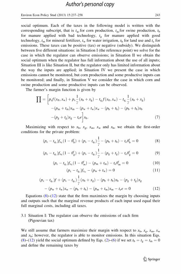
social optimum. Each of the taxes in the following model is written with the

corresponding subscript, that is tqCfor corn production, tqS

for swine production, tbfor manure applied with bad technology, tg for manure applied with good

technology, tm for mineral fertilizer, tw for water irrigation, th for land use and te for

emissions. These taxes can be positive (tax) or negative (subsidy). We distinguish

between five different situations: in Situation I (the reference point) we solve for the

case in which the regulator can observe emissions; in Situation II we obtain the

social optimum when the regulator has full information about the use of all inputs;

Situation III is like Situation II, but the regulator only has limited information about

the way the inputs are applied; in Situation IV we present the case in which

emissions cannot be monitored, but corn production and some productive inputs can

be monitored; and finally, in Situation V we consider the case in which corn and

swine production and some productive inputs can be observed.

The farmer’s margin function is given by

Y¼ pcf ðxft; xwÞ þ ps

1

cðxb þ xgÞ � tqc

f ðxft; xwÞ � tqs

1

cðxb þ xgÞ

�

�ðpm þ tmÞxm � ðpw þ twÞxw � ðph þ thÞ � ðpb þ tbÞxb

�ðpg þ tgÞxg � tee

�xh: ð7Þ

Maximizing with respect to xb, xg, xm, xw and xh, we obtain the first-order

conditions for the private problem:

ðpc � tqcÞfxftð1� h0bÞ þ ðps � tqs

Þ 1c� ðpb þ tbÞ � teh

0b ¼ 0 ð8Þ

ðpc � tqcÞfxftð1� h0gÞ þ ðps � tqs

Þ 1c� ðpg þ tgÞ � teh

0g ¼ 0 ð9Þ

ðpc � tqcÞfxftð1� h0mÞ � ðpm þ tmÞ � teh

0m ¼ 0 ð10Þ

ðpc � tqcÞfxw� ðpw þ twÞ ¼ 0 ð11Þ

ðpc � tqcÞf þ ðps � tqs

Þ 1cðxb þ xgÞ � ðpb þ tbÞxb � ðpg þ tgÞxg

� ðpw þ twÞxw � ðph þ thÞ � ðpm þ tmÞxm � tee ¼ 0 ð12ÞEquations (8)–(12) state that the firm maximizes the margin by choosing inputs

and outputs such that the marginal revenue products of each input used equal their

full marginal costs, including all taxes.

3.1 Situation I: The regulator can observe the emissions of each firm

(Pigouvian tax)

We still assume that farmers maximize their margin with respect to xb, xg, xm, xw

and xh; however, the regulator is able to monitor emissions. In this situation Eqs.

(8)–(12) yield the social optimum defined by Eqs. (2)–(6) if we set tb ¼ tg ¼ tm ¼ 0

and define the remaining taxes by

Environ Econ Policy Stud (2013) 15:237–258 243

123

Author's personal copy

�D0ð�Þh0b ¼ �tqcfxftð1� h0bÞ � tqs

1

c� teh

0b ð13Þ

�D0ð�Þh0g ¼ �tqcfxftð1� h0gÞ � tqs

1

c� teh

0g ð14Þ

�D0ð�Þh0m ¼ �tqcfxftð1� h0mÞ � teh

0m ð15Þ

tw ¼ �tqcfxw

ð16Þ

�D0e ¼ �tqcf � tqs

ðxb þ xgÞc

� twxw � th � tee ð17Þ

From Eqs. (13) and (14) we obtain D0ð�Þ ¼ te � tqcfxft

, which together with (15)

implies that te ¼ D0ð�Þ. Therefore, the remaining taxes tqc; tqs

; tw and th can be

written as

tqc¼ D0ð�Þh0m � teh

0m

fxftð1� h0mÞ

¼ 0 ð18Þ

tqs¼ ½ðD0ð�Þ � teÞh0b�c ¼ 0 ð19Þ

tw ¼ �D0ð�Þh0m � teh

0m

fxftð1� h0mÞ

fxw¼ 0 ð20Þ

th ¼ ðD0 � teÞe ¼ 0: ð21ÞThe usual Pigouvian tax on emissions te is equal to the marginal environmental

damage. If this is the case, then Eqs. (13)–(21) show that there is no need to tax outputs,

inputs or the way the manure is applied to attain the social optimum. Even though the

characteristics of nonpoint source pollution imply that the regulator is not able to

monitor these emissions, we have analysed this case as it provides a reference point for

other policies. In particular, the regulator has to look for other configurations of taxes/

subsidies which can be implemented and that replicate the first-best outcome.

3.2 Situation II The regulator can observe the inputs applied (full information)

In this situation the regulator does not have to be able to observe emissions and the

choice of outputs, i.e. tqc¼ tqs

¼ te ¼ 0. However, the regulator must be able to

monitor the amount of all inputs, more precisely xb, xg, xm, xw and xh, whether they

pollute or not. In this way the substitution processes between all the inputs can be

taken into account. For this reason applying two-part instruments yields the first-

best and not the second-best outcome. In this case the following set of taxes/

subsidies is able to establish the social optimum:

tb ¼ D0h0b [ 0 ð22Þ

tg ¼ D0h0g [ 0 ð23Þ

tm ¼ D0h0m [ 0 ð24Þ

244 Environ Econ Policy Stud (2013) 15:237–258

123

Author's personal copy

tw ¼ �tqcfxw¼ 0 ð25Þ

th ¼ D0ðe� h0bxb � h0gxg � h0mxmÞ\0 ð26Þ

Placing these instruments in Eqs. (8)–(12) shows that these equations generate the

necessary conditions for the social optimum described by Eqs. (2)–(6). Hence, the

two-part instruments defined by Eqs. (22)–(26) are able to induce the social optimum.

Expressions (22)–(25) show that three taxes are strictly positive, and one is zero. In

contrast, the sign of expression (26) cannot be assigned in a straightforward way.

Since the functions hl;l ¼ b; g;m are convex on the interval ½0; x�l � and hlð0Þ ¼ 0, we

have that h0lx�l [ hlðx�l Þ. Consequently, the land-use tax th ¼ D0ð�ÞðhmðxmÞ þ hbðxbÞþ

hgðxgÞ � h0mxm � h0bxb � h0gxgÞ is negative, since D0 is strictly positive. In practical

terms it signifies that the land-use tax is a subsidy. If the emission functions were

linear, or strictly concave, we obtain that h0lx�l � hlðx�l Þ; l ¼ b; g;m. Therefore, in the

case of linear or strictly concave emission functions the land-use tax would be zero or

positive, respectively, i.e. a proper tax. The intuition for a negative land-use tax

(subsidy) resides in the fact that the farmer’s tax expenditures per hectare are D0h0lx�l

where l = b, g, m. However, with respect to land use, the farmers’ tax expenditures

should correspond to the environmental damage times the emissions, i.e.

D0hl; l ¼ b; g;m. Since the emission functions are strictly convex, the difference

between the farmer’s actual tax expenditures and the correct tax expenditures per

hectare is positive, i.e. the farmer pays too much. Hence, the land-use tax is a land-use

subsidy which returns the overpayment to the farmer.

3.3 Situation III: The regulator can observe the amount but not the way inputs

are applied (limited information)

In this situation the regulator is able to observe the amount of all applied inputs, but

cannot distinguish between good and bad manure application practices because this

is the farmer’s private information. This leads to asymmetric information between

the regulator and the farmer. Previous literature has considered adverse selection

models to regulate nonpoint source water pollution where the information about the

type of farming (productivity) is private. These models assume that either the input

(Xepapadeas 1997) or the output (Laffont 1994; Clemenz 1999; Bontems et al.

2005) is observable, and emissions are a function of the unobservable farmer type

and the outputs or inputs. The case studied in Situation III, however, is not covered

by the cited literature since emissions vary for the same amount of input and output

according to the way the manure is applied. Alternatively, Innes (1999) and Macho-

Stadler and Perez-Castrillo (2007) analysed a model in which polluters have the

possibility to report high emissions in exchange for lower taxes. However, this

approach requires that the regulator can determine the emission levels after

inspection at any moment in time. Yet, once the manure is applied the regulator

cannot deduce the way the manure was applied and therefore, this approach is also

not applicable in Situation III.

Since the taxes associated with bad practices are higher than those associated

with good practices, tb [ tg, farmers have incentives to report that they use good

Environ Econ Policy Stud (2013) 15:237–258 245

123

Author's personal copy

practices even if it is not true. Likewise, since the regulator cannot observe the way

manure is applied, he/she cannot impose a differentiated tax according to the

agronomic practices of the farmer. To overcome this adverse selection problem the

regulator may impose a tax of tb on the entire manure, independently of whether

the farmer uses good or bad practices.5 To obtain information about the practices

employed to apply manure, the regulator can create the figure of an accredited

verifier6 who validates that the manure was applied in accordance with good

environmental practices.7 The farmer decides voluntarily to contract or not the

services of the accredited verifier. It can be a firm that applies manure on behalf of

the farmer or a firm that limits its activity to validating the fact that the farmer has

used good environmental practices. In the later case it is in the own interest of the

farmer that the accredited verifier is in the position to observe the application of

good environmental practices, because only then she/he qualifies for a refund. For

simplicity of the exposition, let the costs of the accredited verifier in either case be

denoted by pv. They reflect the difference between the costs of the commissioned

service of the accredited verifier and the cost to farmers of applying the manure

themselves. Once the manure has been applied, the accredited verifier issues a

certificate that shows the amount of manure that has been applied correctly. Farmers

who present this certificate to the regulator receive a refund given by tb � tg for each

kg of correctly applied manure. The amount of the refund (rebate) is equivalent to

the decrease in the marginal environmental damage resulting from the adoption of

good practices tb � tg ¼ D0ð�Þðh0b � h0gÞ[ 0:

In the absence of asymmetric information, Eqs. (22)–(26) together with tqc¼

tqs¼ te ¼ 0 define the taxes/subsidies that achieve the social optimum. Hence, the

additional cost of eliciting the private information is given by pv and is not borne by

the regulator but by the farmer. If the subsidy received tb - tg compensates the

additional cost pv, the farmer is likely to commission the service of the accredited

verifier. Moreover, the remaining two-part instruments, defined in (22)–(26),

guarantee that farmers generate the socially optimal level of manure. Thus, in the

presence of two-part instruments, the net margin of farmers who follow good

5 This approach has some parallels to the principle of ‘‘guilty until proven innocent’’ embodied in the

concept of ‘‘default values’’ in environmental regulation. For example, the Irish Department of the

Environment Heritage and Local Government established, in the absence of verifiable information,

default values for assessing noise pollution. The same spirit gives rise to performance bonds where fees

are levied upon companies that extract certain natural resources, such as timber, coal, oil, and gas.

Amounts deposited with the performance bond can be refunded when the payer fulfils certain obligations.

In that sense, a performance bond acts like a deposit–refund system.6 For example the figure of an ‘‘accredited verifier’’ or certified pesticide applicator is used by the

California Department of Pesticide Regulation. Its licensing and certification programme is responsible

for examining and licensing pest control dealer designated agents, agricultural pest control advisers; and

for certifying pesticide applicators that use or supervise the use of restricted pesticides. For more

information see http://www.cdpr.ca.gov/docs/license/liccert.htm (accessed 06/09/2012). Similar regula-

tions are in place for instance in New York State http://www.labor.state.ny.us/stats/olcny/commercial-

pesticide-applicator-technician.shtm (accessed 06/09/2012), or in British Columbia, Maine and New

Mexico.7 One may ask who supervises and controls the accredited verifier. However, since this question is also

true for any pollution problem (point or nonpoint), it will not be pursued here.

246 Environ Econ Policy Stud (2013) 15:237–258

123

Author's personal copy

practices should be higher than the net margin of those who follow bad practices.

This restriction, as stipulated in the literature on asymmetric information, can be

conceived as an individual rationality constraint. The presence of this constraint is a

clear distinction between traditional economic incentives, such as taxes, subsidies or

tradable permits and two-part instruments. The individual rationality constraint

emerges because the adoption of good practices is completely voluntary and the

reduction in marginal environmental damages (refund/rebate) needs to cover the

costs of the accredited verifier.

If the increase in the SNM resulting from the adoption of good practices does not

cover the costs of the accredited verifier, it is not socially optimal to implement the

proposed two-part instruments, or to introduce the figure of an accredited verifier.

This situation may arise when the reduction in marginal environmental damages is

small, or when the costs of the accredited verifier are high, or both.

It is also possible to relax the assumption that all firms are identical. The Appendix

shows the changes that are necessary to consider heterogeneity of the firms.

3.4 Situation IV: The regulator can observe corn output and some of the inputs

We consider the situation in which the regulator is able to monitor corn production

and some of the inputs, but not all of them, e.g. tqs¼ tm ¼ te ¼ 0. The exclusion of

the tax on mineral fertilizer may be motivated by the fact that although the model

has n identical firms, farms outside the region under consideration probably have

different production functions. It implies that the purchase of mineral fertilizer

would have to be taxed at different rates. But the separation of mineral fertilizer

markets is not recommendable because varying taxes from one region to another

provides incentives for trading of mineral fertilizer on the black market which

undermines the environmental instrument. Along the same lines, the emergence of a

black market for manure is far less likely since the transportation costs are relatively

high. Hence, one can maintain taxes/subsidies on manure following good or bad

practices as an effective instrument. Consequently, the regulator can impose a tax

on corn production, water, land and good and bad practices. Placing these taxes into

the system of Eqs. (8)–(12), the following necessary conditions provide the

equivalence between the private and social outcome.

tb ¼ �D0ð�Þh0mð1� h0mÞ

ð1� h0bÞ þ D0ð�Þh0b 6¼ 0 ð27Þ

tg ¼ �D0ð�Þh0mð1� h0mÞ

ð1� h0gÞ þ D0ð�Þh0g 6¼ 0 ð28Þ

tw ¼ �D0ð�Þh0m

fxftð1� h0mÞ

fxw\0 ð29Þ

tqc¼ D0ð�Þh0m

fxftð1� h0mÞ

[ 0 ð30Þ

Environ Econ Policy Stud (2013) 15:237–258 247

123

Author's personal copy

th ¼ D0ð�Þ½e� h0bxb � h0gxg� þD0ð�Þh0mð1� h0mÞ

� f ð�Þfxft

þ ð1� h0bÞxb þ ð1� h0gÞxg þfxw

fxft

xw

� �

ð31ÞThe results show that the tax on water tw is negative while the tax on corn tqc

is

positive. The taxes on manure have to be applied in the same way as in Situation III

where the rebate for the application of good practices is equal to tb � tg. The tax on

land has to be strictly negative if corn production relies entirely on manure, i.e. no

mineral fertilizer is applied, and hm and h0m are equal to zero. Taking account of the

convexity of the emission function equation (31) yields

th ¼ D0ð�Þ½hb � h0bxb þ hg � h0gxg�\0:

These calculations show that corn output is taxed (deposit) while the non-

polluting input receives a subsidy (refund). However, without particular assump-

tions the sign of Eq. (31) cannot be determined unambiguously, and therefore, we

have complemented our theoretical analysis with an empirical illustration presented

in Sect. 4.

3.5 Situation V: The regulator can observe both outputs and some of the inputs

Finally, we look at the situation where the regulator can observe not only corn but

also swine production along with water and good and bad practices, i.e.

tm ¼ th ¼ te ¼ 0. Placing taxes on corn and swine production, water and good and

bad practices into the system of Eqs. (8)–(12) shows that the tax on swine

production cancels out. To see this isolate tb and tg in Eqs. (8) and (9) and

substitute these term in Eq. (12). Hence, the term tqSwill disappear in the first-

order conditions as a consequence of the linearity of the mathematical

specification of swine production and of the tax on the emissions. As a result

we cannot determine the tax on swine production analytically via the first order

conditions. For the indeterminacy of tqSit does not matter whether we try to solve

for tqCand tqS

, or just for tqSon its own. Nevertheless, we can determine the tax

on swine production empirically because the numerical solution of the

corresponding optimization problem is not based on the solution of the first-

order conditions.

Apart from the five situations presented above, it would have been possible to

analyse more situations; however, we have not presented more situations for the

sake of brevity. In general the choice of which instruments to include and which to

eliminate by setting them to zero depends on the availability, or capacity to monitor

the relevant data. However, since the regulator determines the optimal value of five

variables which gives rise to five first-order conditions, it is not possible to include

more than five from the eight available instruments. In other words, three

instruments have to be set equal to zero to ‘‘guarantee’’ a unique solution. In the

case that the regulator cannot monitor whether farmers follow good or bad practices,

the regulator can overcome the asymmetric information problem by creating the

figure of an accredited verifier as described above.

248 Environ Econ Policy Stud (2013) 15:237–258

123

Author's personal copy

4 Empirical illustration

In this section, we illustrate the previous theoretical results with data from a region

located in north-east Spain. First, we portray the main agricultural characteristics of

the area studied and describe the data employed in the numerical analysis. We also

present the specification of the parameters and functions of the economic model

described above. Then, we interpret the results of the model solution and conduct a

sensitivity analysis of our results with respect to the magnitude of marginal

monetary damages of the nitrogen emissions considered.

4.1 Data and study area

Our study is based in Aragon, an autonomous community in north-east Spain. This

region is one of the main areas of intensive pig farming in Spain. It accounts for

40 % of the total Spanish swine population.8 In the region, pig production represents

54 % of the total livestock production and 28 % of the final value of agricultural

production (Iguacel 2006).

For our numerical analysis we considered the operational costs of an average

farm located in the study area, which represents the behaviour of a farmer with

swine and corn production.9 The specified farm model reproduces the typical

conditions of the region with respect to the farm size and biophysical data, as corn is

one of the main crops grown (see Martınez 2002).

The numerical solution of the mathematical model (Eq. (1)) requires the

functions and parameters to be specified. Relevant data on nitrogen emissions and

management costs of different practices were collected from Iguacel (2006),

Dauden et al. (2004) and Dauden and Quılez (2004). The corn production as a

function of applied nitrogen requires the estimation of function f ðxft; xwÞ of the

model. In order to simplify the estimation process, we determined a new production

function depending directly on xl, l = b, g, m and xw. This function is given by

1ðxb; xg; xm; xwÞ and was previously estimated by Martınez and Goetz (2007) in the

usual quadratic form:

1ðxb; xg; xm; xwÞ ¼ a0 þ a1xf þ a2x2f þ a3xw þ a4x2

w: ð32ÞIn this way we avoided estimating xft first and thereafter f ðxft; xwÞ. The nitrate

emissions as a function of applied nitrogen were specified in the form of:

hj ¼ b0 þ b1xf þ b2x2f with j ¼ b; g;m: ð33Þ

In order to estimate these functions we calibrated the process-oriented

biophysical model Erosion Productivity Impact Calculator (EPIC, Mitchell et al.

1998) to the local conditions and simulated corn production under varying

8 After Germany, Spain has the second largest swine population in the European Union, representing

18 % of the total production in the European Union with a strongly growing trend over the last 10 years

(Dauden and Quılez 2004).9 We consider the case of a farm in a vertically integrated production system, i.e. the farmers’ services

for the fatting of the hogs are commissioned by another firm. It usually provides the incoming animals

and several other inputs of production.

Environ Econ Policy Stud (2013) 15:237–258 249

123

Author's personal copy

conditions. As a result of these simulations we also obtained data about nitrogen

emissions (in the form of nitrate leaching) which allowed us to estimate the

functions hj; j ¼ b; g;m. The simulated data sets obtained with EPIC were validated

by comparing them with crop yields, amounts of inputs applied and nutrient losses

available from an experimental farm of the Department of Soils and Irrigation

(CITA, Aragon Government).10

The results of the estimations of the corn production and nitrate leaching

functions (32 and 33) for mineral fertilizer and good and bad agricultural practices

are presented in Table 1. The parameters of the quadratic functions were estimated

using the nonlinear least-squared regression procedure in SHAZAM (White 2002).

The costs of production and product/input prices were determined based on data

published annually by the Extension Service of the Aragon Government (2005,

2007). The fixed and variable costs of the two ‘‘technologies’’ considered for manure

application, in our example good and bad practices, were obtained from Iguacel and

Yague (2007). The parameter c was assigned a value of 1.57 kg N, based on data

provided by the Extension Service of the Aragon Government (2005, 2007).

Unfortunately, there are no regional data available to estimate the water

treatment costs as a function of nitrate concentration. In accordance with the

literature, the treatment cost function was specified linearly (Tahvonen 1995;

Spraggon 2002). The unitary cost for water treatment is 1.3 €/kg of nitrogen and m3

of water with a targeted concentration below 25 mg of nitrate per litre of water

(Martınez 2002).11 In Table 2 we present the values of the product and input prices

Table 1 Corn production function and nitrate leaching functions

Production

function (~qC)

Nitrate leaching functions

Good

practices (hg)

Bad

practices (hb)

Mineral

fertilizer (hm)

Intercept -2.77 (-6.84)

Lineal water

coefficient (xw)

0.349 9 10-2

(42.90)

Squared water

coefficient (xw2 )

-0.269 9 10-6

(-35.23)

Lineal nitrogen

coefficient (xf)

0.251 9 10-1

(12.21)

0.0344 (6.27) 0.08073 (2.15) 0.0702 (7.21)

Squared nitrogen

coefficient (xf2)

-0.336 9 10-4

(-9.79)

0.113 9 10-3

(5.09)

0.2645 9 10-3

(5.51)

0.23 9 10-3

(4.49)

Adjusted R2 0.86 0.87 0.89 0.85

t statistics are shown in parentheses

10 See Dauden et al. (2004) and Dauden and Quılez (2004) for the physical characteristics of the

experimental farm and details on the conditions of the field trial conducted for the calculation of the

nutrient losses.11 Foess et al. (1998) compared the cost of different processes applied in the USA to remove biological

nutrients from water, and reported water treatment costs that range from 1.4 to 21 US$/m3. The large cost

discrepancy with respect to our cost can be explained in part because the costs considered here are

independent of the pre-treatment nitrate level.

250 Environ Econ Policy Stud (2013) 15:237–258

123

Author's personal copy

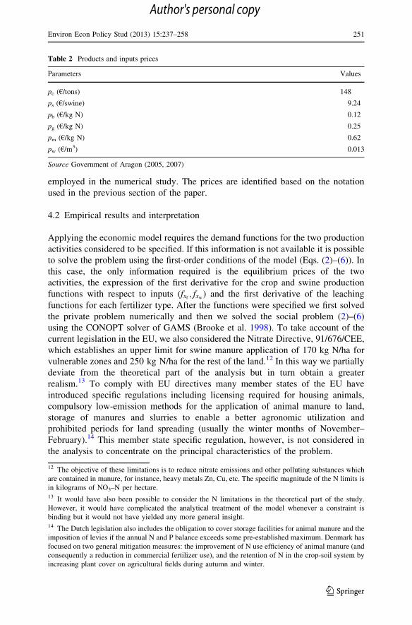
employed in the numerical study. The prices are identified based on the notation

used in the previous section of the paper.

4.2 Empirical results and interpretation

Applying the economic model requires the demand functions for the two production

activities considered to be specified. If this information is not available it is possible

to solve the problem using the first-order conditions of the model (Eqs. (2)–(6)). In

this case, the only information required is the equilibrium prices of the two

activities, the expression of the first derivative for the crop and swine production

functions with respect to inputs (fxf; fxw

) and the first derivative of the leaching

functions for each fertilizer type. After the functions were specified we first solved

the private problem numerically and then we solved the social problem (2)–(6)

using the CONOPT solver of GAMS (Brooke et al. 1998). To take account of the

current legislation in the EU, we also considered the Nitrate Directive, 91/676/CEE,

which establishes an upper limit for swine manure application of 170 kg N/ha for

vulnerable zones and 250 kg N/ha for the rest of the land.12 In this way we partially

deviate from the theoretical part of the analysis but in turn obtain a greater

realism.13 To comply with EU directives many member states of the EU have

introduced specific regulations including licensing required for housing animals,

compulsory low-emission methods for the application of animal manure to land,

storage of manures and slurries to enable a better agronomic utilization and

prohibited periods for land spreading (usually the winter months of November–

February).14 This member state specific regulation, however, is not considered in

the analysis to concentrate on the principal characteristics of the problem.

Table 2 Products and inputs prices

Parameters Values

pc (€/tons) 148

ps (€/swine) 9.24

pb (€/kg N) 0.12

pg (€/kg N) 0.25

pm (€/kg N) 0.62

pw (€/m3) 0.013

Source Government of Aragon (2005, 2007)

12 The objective of these limitations is to reduce nitrate emissions and other polluting substances which

are contained in manure, for instance, heavy metals Zn, Cu, etc. The specific magnitude of the N limits is

in kilograms of NO3–N per hectare.13 It would have also been possible to consider the N limitations in the theoretical part of the study.

However, it would have complicated the analytical treatment of the model whenever a constraint is

binding but it would not have yielded any more general insight.14 The Dutch legislation also includes the obligation to cover storage facilities for animal manure and the

imposition of levies if the annual N and P balance exceeds some pre-established maximum. Denmark has

focused on two general mitigation measures: the improvement of N use efficiency of animal manure (and

consequently a reduction in commercial fertilizer use), and the retention of N in the crop-soil system by

increasing plant cover on agricultural fields during autumn and winter.

Environ Econ Policy Stud (2013) 15:237–258 251

123

Author's personal copy

In Table 3 we present the values of the relevant variables obtained by solving the

private and social decision problems with a limit of 250 kg N/ha and with no

limitation. Basically, the differences between the private and social outcomes refer

to the use of manure: in comparison with the private solution, the social optimum

requires reducing the amount of manure applied following bad practices, increasing

the amount of manure and mineral fertilizer applied following good practices.

Table 3 shows that farmers without N limitations do not apply mineral fertilizer at

all because it leads to acquisition costs, whereas organic fertilizer is costless.

Without N limitations the private optimum is characterized by the application of

manure following bad practices and no application of mineral fertilizer at all. Upon

imposing N limitations, farmers reduce the amount of manure and substitute it by

the application of mineral fertilizer. In the absence of any N limitations the privately

optimal nitrogen emissions per hectare need to be decreased by approximately 30 %

to achieve the socially optimal nitrogen emission. The farmer’s margin per hectare

without taking account of taxes and subsidies decreases by 3–4 % if the social

outcome is realized.

For the rest of the numerical study we concentrate on the case were the N

limitations are not binding for the sake of the brevity of the exposition.15 To

establish the social optimum we have designed the two-part instruments described

above to induce the adoption of good practices. In our numerical study, we

calculated the two-part instruments for the previously described situations given a

Table 3 Results for the private and the social problem with and without N limits

Variables Without limitation With limitation

Private

problem

Social problem Private

problem

Social problem

Corn production (~qC) in

tons/ha

13.7 13.7 13.7 13.7

Swine production (~qS) per ha 110 101.25 67 66

Nitrogen applied with bad

practices (xb) in kg N/ha

431.5 190.4 250 152.4

Nitrogen applied with good

practices (xg) in kg N/ha

0.0 183.6 0.0 94.3

Mineral nitrogen applied (xm)

in kg N/ha

0.0 0.0 61.7 53.2

Total nitrogen applied

in kg N/ha

431.5 374 311.7 300

Water applied (xw) in m3/ha 6470 6470 6323 6323

Total emissions (e) in kg N/ha 269 180 166.6 90

Margin of the farm (in €/ha)

(in brackets SNM)

2903.7

(2554.1)

2807.8 (no taxes/

subsidies) (2573.8)

2531.8

(2315.2)

2512.5 (no taxes/

subsidies) (2395.5)

15 The result for the case where the N-limit is in place does not vary significantly from the presented

results. The corresponding tables can be obtained from the authors upon request.

252 Environ Econ Policy Stud (2013) 15:237–258

123

Author's personal copy

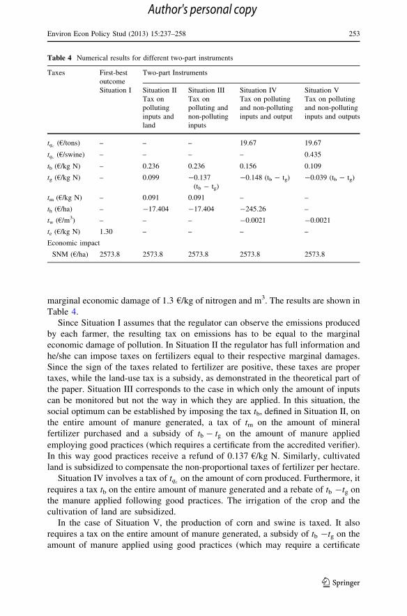
marginal economic damage of 1.3 €/kg of nitrogen and m3. The results are shown in

Table 4.

Since Situation I assumes that the regulator can observe the emissions produced

by each farmer, the resulting tax on emissions has to be equal to the marginal

economic damage of pollution. In Situation II the regulator has full information and

he/she can impose taxes on fertilizers equal to their respective marginal damages.

Since the sign of the taxes related to fertilizer are positive, these taxes are proper

taxes, while the land-use tax is a subsidy, as demonstrated in the theoretical part of

the paper. Situation III corresponds to the case in which only the amount of inputs

can be monitored but not the way in which they are applied. In this situation, the

social optimum can be established by imposing the tax tb, defined in Situation II, on

the entire amount of manure generated, a tax of tm on the amount of mineral

fertilizer purchased and a subsidy of tb � tg on the amount of manure applied

employing good practices (which requires a certificate from the accredited verifier).

In this way good practices receive a refund of 0.137 €/kg N. Similarly, cultivated

land is subsidized to compensate the non-proportional taxes of fertilizer per hectare.

Situation IV involves a tax of tqcon the amount of corn produced. Furthermore, it

requires a tax tb on the entire amount of manure generated and a rebate of tb -tg on

the manure applied following good practices. The irrigation of the crop and the

cultivation of land are subsidized.

In the case of Situation V, the production of corn and swine is taxed. It also

requires a tax on the entire amount of manure generated, a subsidy of tb -tg on the

amount of manure applied using good practices (which may require a certificate

Table 4 Numerical results for different two-part instruments

Taxes First-best

outcome

Two-part Instruments

Situation I Situation II

Tax on

polluting

inputs and

land

Situation III

Tax on

polluting and

non-polluting

inputs

Situation IV

Tax on polluting

and non-polluting

inputs and output

Situation V

Tax on polluting

and non-polluting

inputs and outputs

tqc(€/tons) – – – 19.67 19.67

tqs(€/swine) – – – – 0.435

tb (€/kg N) – 0.236 0.236 0.156 0.109

tg (€/kg N) – 0.099 -0.137

(tb - tg)

-0.148 (tb - tg) -0.039 (tb - tg)

tm (€/kg N) – 0.091 0.091 – –

th (€/ha) – -17.404 -17.404 -245.26 –

tw (€/m3) – – – -0.0021 -0.0021

te (€/kg N) 1.30 – – – –

Economic impact

SNM (€/ha) 2573.8 2573.8 2573.8 2573.8 2573.8

Environ Econ Policy Stud (2013) 15:237–258 253

123

Author's personal copy

from the accredited verifier) and a subsidy per unit of water applied. Imposing a tax

on the two outputs allows the tax on mineral fertilizer and land use to be suppressed.

A comparison of the SNM for the three situations confirms that the two-part

instruments are capable of replicating the social optimum.

In addition, we conducted a sensitivity analysis of the values of the marginal

environmental damage caused by nitrate emissions. We increased water treatment

costs from 1 to 2.5 €/kg of nitrate. Figure 1 illustrates the change in the use of good

and bad practices when the marginal economic damage of pollution increases. As

expected, the use of good practices expands as the social damage of emissions

increases (see Fig. 1).

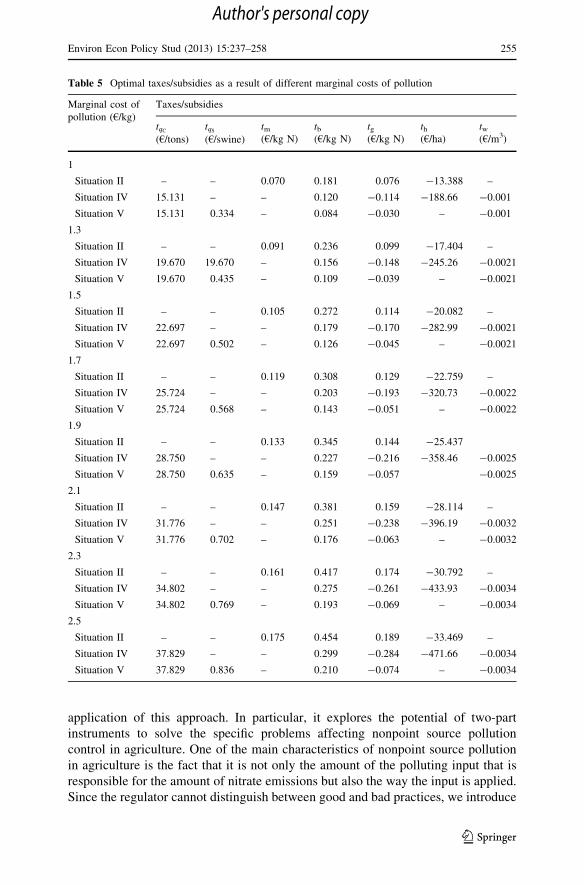
In Table 5 we also present the corresponding two-part instruments for Situations

II, IV and V under different marginal costs of pollution (water treatment costs). As

the marginal economic damage of pollution increases, both taxes and subsidies

increase. The difference between taxes and subsidies increases in absolute but not in

relative terms as the marginal environmental damage increases, since the marginal

environmental damage is constant.

Moreover, for Situations II, IV and V we calculated the values of the elasticities

for all the taxes and subsidies with respect to the marginal environmental damage.

The calculated values are in the range of j0:8j to j1:1j; implying that the variation in

the marginal environmental cost considered leads to a proportional variation in the

taxes or subsidies.

5 Conclusions

Since nonpoint source emissions cannot be attributed to particular polluters, a first-

best tax on nitrate emissions is not a viable option for policy makers. Alternatively,

a mix of pure environmental regulations in the form of two-part instruments can be

designed to obtain combinations of taxes and subsidies on observable inputs and

outputs that induce the socially optimal level of pollution. These voluntary but

economic incentive-based instruments maintain most of the properties of a first-best

Pigouvian tax while minimizing the need for monitoring and enforcement. Our

analysis aims to contribute to the literature with respect to the design and

0

50

100

150

200

250

300

1 1.3 1.5 1.7 1.9 2.1 2.3 2.5

Marginal cost ofpollution( /kg)

Ap

plie

d m

anu

re (

kg/h

a)

Bad practices Good practices

Fig. 1 The socially optimal levels of manure applied using good and bad practices for different levels ofthe marginal cost of pollution

254 Environ Econ Policy Stud (2013) 15:237–258

123

Author's personal copy

application of this approach. In particular, it explores the potential of two-part

instruments to solve the specific problems affecting nonpoint source pollution

control in agriculture. One of the main characteristics of nonpoint source pollution

in agriculture is the fact that it is not only the amount of the polluting input that is

responsible for the amount of nitrate emissions but also the way the input is applied.

Since the regulator cannot distinguish between good and bad practices, we introduce

Table 5 Optimal taxes/subsidies as a result of different marginal costs of pollution

Marginal cost of

pollution (€/kg)

Taxes/subsidies

tqC

(€/tons)

tqS

(€/swine)

tm(€/kg N)

tb(€/kg N)

tg(€/kg N)

th(€/ha)

tw(€/m3)

1

Situation II – – 0.070 0.181 0.076 -13.388 –

Situation IV 15.131 – – 0.120 -0.114 -188.66 -0.001

Situation V 15.131 0.334 – 0.084 -0.030 – -0.001

1.3

Situation II – – 0.091 0.236 0.099 -17.404 –

Situation IV 19.670 19.670 – 0.156 -0.148 -245.26 -0.0021

Situation V 19.670 0.435 – 0.109 -0.039 – -0.0021

1.5

Situation II – – 0.105 0.272 0.114 -20.082 –

Situation IV 22.697 – – 0.179 -0.170 -282.99 -0.0021

Situation V 22.697 0.502 – 0.126 -0.045 – -0.0021

1.7

Situation II – – 0.119 0.308 0.129 -22.759 –

Situation IV 25.724 – – 0.203 -0.193 -320.73 -0.0022

Situation V 25.724 0.568 – 0.143 -0.051 – -0.0022

1.9

Situation II – – 0.133 0.345 0.144 -25.437

Situation IV 28.750 – – 0.227 -0.216 -358.46 -0.0025

Situation V 28.750 0.635 – 0.159 -0.057 -0.0025

2.1

Situation II – – 0.147 0.381 0.159 -28.114 –

Situation IV 31.776 – – 0.251 -0.238 -396.19 -0.0032

Situation V 31.776 0.702 – 0.176 -0.063 – -0.0032

2.3

Situation II – – 0.161 0.417 0.174 -30.792 –

Situation IV 34.802 – – 0.275 -0.261 -433.93 -0.0034

Situation V 34.802 0.769 – 0.193 -0.069 – -0.0034

2.5

Situation II – – 0.175 0.454 0.189 -33.469 –

Situation IV 37.829 – – 0.299 -0.284 -471.66 -0.0034

Situation V 37.829 0.836 – 0.210 -0.074 – -0.0034

Environ Econ Policy Stud (2013) 15:237–258 255

123

Author's personal copy

the figure of an accredited verifier to overcome the associated asymmetric

information problem. This requires farmers to pay the tax that corresponds to using

bad practices on the entire manure generated at the farm. Only farmers that present a

certificate issued by the accredited verifier, stating the amount of manure and that it

has been applied using good practices, receive the subsidy for this amount of

manure.

In particular, we have found that there are many ways of achieving the social

optimum: a combination of taxes on polluting inputs and a subsidy on land use, or a

combination of taxes on outputs and bad practices while subsidizing a non-polluting

input and good practices. Finally, the analysis presented in this paper shows how

economic incentives can be designed to improve acceptance of the best manage-

ment practices.

Acknowledgments The authors gratefully acknowledge the support of the Ministerio de Ciencia e

Innovacion Grants Econ2010-17020, and RTA2010-00109-C04-01 and of the Government of Catalonia

(Barcelona Graduate School of Economics, Grants XREPP, and 2009 SGR189).

Appendix: Heterogeneity of the firms

So far we have assumed that the n firms are identical. If we drop this assumption we

can classify the firms in k groups. The firms that belong to group j, j ¼ 1; . . .; k; have

identical characteristics, i.e. they can be described by the same production function

f jð�Þ, the same emission function h jl ð�Þ; l ¼ b; g;m, the same production and

application cost of manure pjb and p

jb and by the number of firms nj that form part of

group j. The choice variables of each firm of group j are given by xjb; x

jg; x

jm; x

jw; and

xjh: Consequently the social decision problem reads as

ZPk

j¼1

f jðx j

ft;x j

wÞnjxj

h

0

pcðqcÞdqc þZ

Pk

j¼1

ðx j

bþx

jgÞnjx

j

h=c

0

psðqsÞdqs

� njxjh½pwx j

w þ pmx jm þ p

jbx

jb þ p j

gx jg þ ph� � D

Xk

j¼1

njxjhe j

!

Adapting the notation also for the farmer’s margin function and following the

steps described above, we obtain that the first-order conditions for the social and

private problems. A comparison of these conditions allows us to determine group

specific taxes t jqc; t j

qs; t j

b; tjg; t

jm; t

jw; t

jh so that farmers faced with these taxes would

behave optimally from a social point of view. These taxes would respond to

Situation II.

However, the deriving the optimal taxes requires that the social planner knows

the production and emission functions of each group j as well as the different costs

of swine production and the application of the manure. Assume that the regulator

only knows the emission function of each group j, but not the production function

256 Environ Econ Policy Stud (2013) 15:237–258

123

Author's personal copy

and costs of each group. In the case that the regulator knows the distribution of the

production functions and costs over all groups a permit trading scheme for manure

applied following good practices can be implemented. More precisely, the regulator

knows the functions f jð�Þ, the values of pjb, p

jb, nj and the share of each group j with

respect to all firms. Furthermore, it is necessary that the regulator has established an

accredited verification system for good practices. Within this setting, the regulator

can calculate the optimal application of all inputs for the entire sector, but not for

each individual firm. Consequently, the regulator can determine the optimal

emissions of the entire sector that result from the application of manure following

bad practices E�b and following good practices E�g. The quantity E�b can be

approximated by imposing a tax t�b on manure that corresponds to the average

marginal damage of manure over all groups. The quantity E�g can be established by a

permit trading system for manure applied following good practices. The exchange

of the permits has to be weighted by the differences in the emission function of each

group, i.e. if one kg of manure applied following good practices in group 1 results in

twice as much emissions as in group 2, firms in group 1 have to have twice as many

permits as firms in group 2 given the same amount of manure. The price of the

permits is established in the market, and the participating firms get a refund of t�b.

The conditions for this scheme are outlined at the beginning of the section

Situation III.

References

Abdalla C, Borisova T, Parker D, Saacke Blunck K (2007) Water quality credit trading and agriculture:

recognizing the challenges and policy issues ahead. Choices 22(2):117–124

Bontems P, Rotillon G, Turpin N (2005) Self-selecting agro-environmental policies with an application to

the Don Watershed. Environ Resour Econ 31(3):275–301

Brooke A, Kendrick D, Meeraus A, Raman R (1998) GAMS tutorial by R. Rosenthal. GAMS

Development Corporation, Washington

Clemenz G (1999) Adverse selection and Pigou taxes. Environ Resour Econ 13(1):13–29

Dauden A, Quılez D (2004) Pig slurry versus mineral fertilization on corn yield and nitrate leaching in a

Mediterranean irrigated environment. Eur J Agron 21:7–19

Dauden A, Quılez D, Vera MV (2004) Pig slurry application and irrigation effects on nitrate leaching in

Mediterranean soil lysimeters. J Environ Qual 33:2290–2295

Dosi C, Tomasi T (1994) Nonpoint source pollution regulation: issues and analysis. Kluwer, Dordrecht

Foess GW, Steinbrecher P, Williams K, Garret GS (1998) Cost and performance evaluation of BNR

processes. Fla Water Res J December:11–16

Fullerton D, Wolverton A (1999) The case for a two-part instrument: presumptive tax and environmental

subsidy. In: Portney PR, Schwab RM (eds) Environmental economics and public policy: essays in

honor of Wallace E. Oates. Elgar, Cheltenham

Fullerton D, Wolverton A (2000) Two generalizations of a deposit–refund system. Am Econ Rev

90(2):238–242

Fullerton D, Wolverton A (2005) The two-part instrument in a second-best world. J Public Econ

89(9–10):1961–1975

Government of Aragon (2005) Anuario Estadıstico Agrario de Aragon. Departamento de Agricultura y

Alimentacion, Zaragoza

Government of Aragon (2007) Anuario Estadıstico Agrario de Aragon. Departamento de Agricultura y

Alimentacion, Zaragoza

Environ Econ Policy Stud (2013) 15:237–258 257

123

Author's personal copy

Iguacel F (2006) Estiercoles y fertilizacion nitrogenada. In: Orus F (ed) Fertilizacion Nitrogenada, Guıa

de actualizacion. Informaciones tecnicas, numero extraordinario. Departamento de Agricultura y

Alimentacion, Gobierno de Aragon, Zaragoza

Iguacel F, Yague MR (2007) Evaluacion de costes de sistemas y equipos de aplicacion de purın (datos

preliminares). Informaciones tecnicas n� 178. Departamento de Agricultura y Alimentacion,

Gobierno de Aragon

Innes R (1999) Remediation and self-reporting in optimal law enforcement. J Public Econ 72:379–393

Laffont J (1994) Regulation of pollution with asymmetric information. In: Graham-Tomasi T, Dosi C

(eds) Nonpoint source pollution regulation. Kluwer, Dordrecht

Lankoski J, Lichtenberg E, Ollikainen M (2010) Agri-environmental program compliance in a

heterogeneous landscape. Environ Res Econ 47:1–22

Macho-Stadler I, Perez-Castrillo D (2007) Optimal monitoring to implement clean technologies when

pollution is random. CESifo Working Paper No. 1966

Martinez Y (2002) Analisis economico y ambiental de la contaminacion por nitratos en el regadıo. Ph.D.

dissertation, University of Zaragoza

Martınez Y, Goetz RU (2007) Ganancias de eficiencia versus costes de transaccion de los mercados de

agua. Revista de Economıa Aplicada XV(43):49–70

Millock K, Sunding D, Zilberman D (2002) Regulating pollution with endogenous monitoring. J Environ

Econ Manag 44:221–241

Millock K, Xabadia A, Zilberman D (2012) Investment policy for new environmental monitoring

technologies to manage stock externalities. J Environ Econ Manag 64:102–116

Mitchell G, Griggs R, Benson V, Williams J (1998) The EPIC model: environmental policy integrated

climate. Texas Agricultural Experiment Station, Temple

Palmer K, Walls M (1997) Optimal policies for solid waste disposal: taxes, subsidies, and standards.

J Public Econ 65:193–205

Panagopoulos Y, Makropoulos C, Mimikou M (2011) Reducing surface water pollution through the

assessment of the cost-effectiveness of BMPs at different spatial scales. J Environ Manag

92:2823–2835

Rao NS, Easton ZM, Schneiderman EM, Zion MS, Lee DR, Steenhuis TS (2009) Modeling watershed-

scale effectiveness of agricultural best management practices to reduce phosphorus loading.

J Environ Manag 90(3):1385–1395

Segerson K, Wu J (2006) Nonpoint pollution control: introducing first-best outcomes through the use of

threats. J Environ Econ Manag 51:165–184

Shortle JS, Abler DG (1998) Nonpoint pollution. In: Folmer H, Tietenberg T (eds) Yearbook of

environmental and resource economics 1997/1998. Edward Elgar, Cheltenham

Spraggon J (2002) Exogenous targeting instruments as a solution to group moral hazards. J Public Econ

84:427–456

Tahvonen O (1995) Dynamics of pollution control when damage is sensitive to the rate of pollution

accumulation. Environ Res Econ 5(1):9–27

Walls M, Palmer K (2001) Upstream pollution, downstream waste disposal, and the design of

comprehensive environmental policies. J Environ Econ Manag 41:94–108

White KJ (2002) SHAZAM—for windows, version 9.0

Xepapadeas AP (1997) Regulation of mineral emissions under asymmetric information. In: Romstad E,

Simonsen J, Vatn A (eds) Controlling mineral emissions in European agriculture. CAB

International, New York

258 Environ Econ Policy Stud (2013) 15:237–258

123

Author's personal copy