Nonparametric Statistics with Applications to Science and Engineering Paul H. Kvam Georgia Institute of Technology The H. hlilton Stewart School oflndustrial and Systems Engineering Atlanta. GA Brani Vidakovic Georgia Institute of Technology and Emory University School of Medicine The Wallace H. Coulter Department of Biomedical Engineering Atlanta, GA BICENTENNIAL BICENTENNIAL WILEY-INTERSCIENCE A John Wiley & Sons, Inc., Publication

Welcome message from author
This document is posted to help you gain knowledge. Please leave a comment to let me know what you think about it! Share it to your friends and learn new things together.
Transcript

Nonparametric Statistics with Applications to
Science and Engineering
Paul H. Kvam Georgia Institute of Technology
The H. hlilton Stewart School oflndustrial and Systems Engineering Atlanta. GA
Brani Vidakovic Georgia Institute of Technology and Emory University School of Medicine
The Wallace H. Coulter Department of Biomedical Engineering Atlanta, GA
B I C E N T E N N I A L
B I C E N T E N N I A L
WILEY-INTERSCIENCE A John Wiley & Sons, Inc., Publication

Copyright 0 2007 by John Wiley & Sons, Inc. All rights reserved.
Published by John Wiley & Sons, Inc., Hoboken, New Jersey Published simultaneously in Canada.
No part of this publication may be reproduced. stored in a retrieval system, or transmitted in any form or by any means, electronic, mechanical, photocopying, recording, scanning, or otherwise, except as permitted under Section 107 or 108 of the 1976 United States Copyright Act, without either the prior written permission of the Publisher, or authorization through payment of the appropriate per-copy fee to the Copyright Clearance Center, Inc., 222 Rosewood Drive, Danvers, MA 01923, (978) 750-8400, fax (978) 750-4470, or on the web at www.copyright.com. Requests to the Publisher for permission should be addressed to the Permissions Department, John Wiley & Sons, Inc., 11 1 River Street, Hoboken, NJ 07030, (201) 748-601 1, fax (201) 748-6008, or online at http://www.wiley.comlgo/permission.
Limit of Liability/Disclaimer of Warranty: While the publisher and author have used their best efforts in preparing this book, they make no representations or warranties with respect to the accuracy or completeness of the contents of this book and specifically disclaim any implied warranties of merchantability or fitness for a particular purpose. No warranty may be created or extended by sales representatives or written sales materials. The advice and strategies contained herein may not be suitable for your situation. You should consult with a professional where appropriate. Neither the publisher nor author shall be liable for any loss of profit or any other commercial damages, including but not limited to special, incidental, consequential, or other damages.
For general information on our other products and services or for technical support, please contact our Customer Care Department within the United States at (800) 762-2974, outside the United States at (317) 572-3993 or fax (317) 572-4002.
Wiley also publishes its books in a variety of electronic formats. Some content that appears in print may not be available in electronic format. For information about Wiley products, visit our web site at www.wiley.com.
Wiley Bicentennial Logo: Richard J. Pacific0
Library of Congress Cataloging-in-Publication Data is available.
ISBN 978-0-470-08 147-1
Printed in the United States of America
I 0 9 8 7 6 5 4 3 2 1

Contents
Preface
1 Introduction 1.1 Efficiency of Nonparametric Methods 1.2 Overconfidence Bias 1.3 Computing with MATLAB 1.4 Exercises References
2 Probability Basics 2.1 Helpful Functions 2.2 2.3 2.4 Discrete Distributions 2.5 Continuous Distributions 2.6 Mixture Distributions 2.7 Exponential Family of Distributions 2.8 Stochastic Inequalities 2.9 Convergence of Random Variables
Events, Probabilities and Random Variables Numerical Characteristics of Random Variables
xi
9 9
11 12 14 17 23 25 26 28
V

vi CONTENTS
2.10 Exercises References
31 32
3 Statistics Basics 3.1 Estimation 3.2 Empirical Distribution Function 3.3 Statistical Tests 3.4 Exercises References
4 Bayesian Statistics 4.1 The Bayesian Paradigm 4.2 Ingredients for Bayesian Inference 4.3 4.4 Exercises References
Bayesian Computation and Use of WinBUGS
5 Order Statistics 5.1 5.2 Sample Quantiles 5.3 Tolerance Intervals 5.4 5.5 Extreme Value Theory 5.6 Ranked Set Sampling 5.7 Exercises References
Joint Distributions of Order Statistics
Asymptotic Distributions of Order Statistics
6 Goodness of Fit 6.1 Kolmogorov-Smirnov Test Statistic 6.2 6.3 Specialized Tests 6.4 Probability Plotting 6.5 Runs Test 6.6 AIeta Analysis 6.7 Exercises
Smirnov Test to Compare Two Distributions
33 33 34 36 45 46
47 47 48 61 63 67
69 70 72 73 75 76 76 77 80
81 82 86 89 97
100 106 109

CONTENTS vii
References
7 Rank Tests 7.1 Properties of Ranks 7.2 Sign Test 7.3 7.4 Wilcoxon Signed Rank Test 7.5 7.6 Mann-Whitney U Test 7.7 Test of Variances 7.8 Exercises References
Spearman Coefficient of Rank Correlation
Wilcoxon (Two-Sample) Sum Rank Test
8 Designed Experiments 8.1 Kruskal-Wallis Test 8.2 Friedman Test 8.3 8.4 Exercises References
Variance Test for Several Populations
9 Categorical Data 9.1 Chi-square and Goodness-of-Fit 9.2 Contingency Tables 9.3 Fisher Exact Test 9.4 MCNemar Test 9.5 Cochran’s Test 9.6 Mantel-Haenszel Test 9.7 CLT for Multinomial Probabilities 9.8 Simpson’s Paradox 9.9 Exercises References
10 Estimating Distribution Functions 10.1 Introduction 10.2 Nonparametric Maximum Likelihood
113
115 117 118 122 126 129 131 133 135 139
141 141 145 148 149 152
153 155 159 163 164 167 167 171 172 173 180
183 183 184

viii CONTENTS
10.3 Kaplan-Meier Estimator 10.4 Confidence Interval for F 10.5 Plug-in Principle 10.6 Semi- P ar ame tric Inference 10.7 Empirical Processes 10.8 Empirical Likelihood 10.9 Exercises References
11 Density Estimation 11.1 Histogram 11.2 Kernel and Bandwidth 11.3 Exercises References
12 Beyond Linear Regression 12.1 Least Squares Regression 12.2 Rank Regression 12.3 Robust Regression 12.4 Isotonic Regression 12.5 Generalized Linear Models 12.6 Exercises References
13 Curve Fitting Techniques 13.1 Kernel Estimators 13.2 Nearest Neighbor Methods 13.3 Variance Estimation 13.4 Splines 13.5 Summary 13.6 Exercises References
14 Wavelets 14.1 Introduction to Wavelets
185 192 193 195 197 198 201 203
205 206 207 213 215
217 218 219 22 1 227 230 237 240
241 243 247 249 251 257 258 260
263 263

CONTENTS ;x
14.2 How Do the Wavelets Work? 14.3 Wavelet Shrinkage 14.4 Exercises References
15 Bootstrap 15.1 Bootstrap Sampling 15.2 Nonparametric Bootstrap 15.3 Bias Correction for Nonparametric Intervals 15.4 The Jackknife 15.5 Bayesian Bootstrap 15.6 Permutation Tests 15.7 More on the Bootstrap 15.8 Exercises References
16 EM Algorithm 16.1 Fisher’s Example 16.2 Mixtures 16.3 EM and Order Statistics 16.4 MAP via EM 16.5 Infection Pattern Estimation 16.6 Exercises References
17 Statistical Learning 17.1 Discriminant Analysis 17.2 Linear Classification Models 17.3 Nearest Neighbor Classification 17.4 Neural Networks 17.5 Binary Classification Trees 17.6 Exercises References
18 Nonparametric Bayes
266 2 73 281 283
285 285 287 292 295 296 298 302 302 304
307 309 311 315 317 318 319 32 1
323 324 326 329 333 338 346 346
349

x CONTENTS
18.1 Dirichlet Processes 18.2 Bayesian Categorical Models 18.3 Infinitely Dimensional Problems 18.4 Exercises References
A MATLAB A . l Using MATLAB A.2 Matrix Operations A.3 Creating Functions in MATLAB A.4 Importing and Exporting Data A.5 Data Visualization A.6 Statistics
B WinBUGS B. l Using WinBUGS B.2 Built-in Functions
hIATLAB Index
Author Index
350 357 360 364 366
369 369 372 374 375 380 386
397 398 40 1
405
409
Subject Index 413

Preface
Danger lies not in what we don't know-. but in what we think we know that just ain't so.
Mark Twain (1835 - 1910)
As Prefaces usually start. the author(s) explain why they wrote the book in the first place ~ and we will follow this tradition. Both of us taught the graduate course on nonparametric statistics at the School of Industrial and Systems Engineering at Georgia Tech (ISyE 6404) several times. The audi- ence was always versatile: PhD students in Engineering Statistics. Electrical Engineering, Management, Logistics, Physics. to list a few. While comprising a non homogeneous group. all of the students had solid mathematical, pro- gramming and statistical training needed to benefit from the course. Given such a nonstandard class. the text selection was all but easy.
There are plenty of excellent monographs/texts dealing with nonparamet- ric statistics, such as the encyclopedic book by Hollander and Wolfe. Non- parametrac Statzstzcal Methods. or the excellent evergreen book by Conover. Practacal Nonparametrzc Statastacs, for example. We used as a text the 3rd edition of Conover's book, which is mainly concerned with what most of us think of as traditional nonparametric statistics: proportions. ranks. categor- ical data. goodness of fit. and so on, with the understanding that the text would be supplemented by the instructor's handouts. Both of us ended up supplying an increasing number of handouts every year, for units such as den- sity and function estimation. wavelets. Bayesian approaches to nonparametric problems. the EM algorithm. splines, machine learning, and other arguably
XI

xi/ PREFACE
modern nonparametric topics. About a year ago. we decided to merge the handouts and fill the gaps.
There are several novelties this book provides. We decided to intertwine informal comments that might be amusing. but tried to have a good balance. One could easily get carried away and produce a preface similar to that of celebrated Barlow and Proschan's, Statastacal Theory of Relaabalzty and Lzfe Testang: Probabzlaty Models, who acknowledge greedy spouses and obnoxious children as an impetus to their book writing. In this spirit. we featured pho- tos and sometimes biographic details of statisticians who made fundamental contributions to the field of nonparametric statistics, such as Karl Pearson. Nathan hfantel, Brad Efron, and Baron Von Munchausen.
Computing. Another specificity is the choice of computing support. The book is integrated with MATLAB@ and for many procedures covered in this book. hfATLAB's m-files or their core parts are featured. The choice of software was natural: engineers. scientists, and increasingly statisticians are communicating in the "AlATLAB language." This language is, for example, taught at Georgia Tech in a core computing course that every freshman engi- neering student takes. and almost everybody around us "speaks MATLAB." The book's website:
http://www2.isye.gatech.edu/NPbook
contains most of the m-files and programming supplements easy to trace and download. For Bayesian calculation we used N-inBUGS, a free software from Cambridge's Biostatistics Research Unit. Both MATLAB and WinBUGS are briefly covered in two appendices for readers less familiar with them.
Outline of Chapters. For a typical graduate student to cover the full breadth of this textbook, two semesters would be required. For a one-semester course. the instructor should necessarily cover Chapters 1-3, 5-9 to start. Depending on the scope of the class, the last part of the course can include different chapter selections.
Chapters 2-4 contain important background material the student needs to understand in order to effectively learn and apply the methods taught in a nonparametric analysis course. Because the ranks of observations have special importance in a nonparametric analysis, Chapter 5 presents basic results for order statistics and includes statistical methods to create tolerance intervals.
Traditional topics in estimation and testing are presented in Chapters 7- 10 and should receive emphasis even to students who are most curious about advanced topics such as density estimation (Chapter 11). curve-fitting (Chap- ter 13) arid wavelets (Chapter 14). These topics include a core of rank tests that are analogous to common parametric procedures (e.g.. t-tests, analysis of variance).
Basic methods of categorical data analysis are contained in Chapter 9. Al-

PREFACE xi;;
though most students in the biological sciences are exposed to a wide variety of statistical methods for categorical data. engineering students and other stu- dents in the physical sciences typically receive less schooling in this quintessen- tial branch of statistics. Topics include methods based on tabled data. chi- square tests and the introduction of general linear models. Also included in the first part of the book is the topic of "goodness of fit" (Chapter 6), which refers to testing data not in terms of some unknown parameters, but the un- known distribution that generated it. In a way. goodness of fit represents an interface between distribution-free methods and traditional parametric meth- ods of inference, and both analytical and graphical procedures are presented. Chapter 10 presents the nonparametric alternative to maximum likelihood estimation and likelihood ratio based confidence intervals.
The term "regression" is familiar from your previous course that introduced you to statistical methods. Konparametric regression provides an alternative method of analysis that requires fewer assumptions of the response variable. In Chapter 12 we use the regression platform to introduce other important topics that build on linear regression. including isotonic (constrained) regression, robust regression and generalized linear models. In Chapter 13. we introduce more general curve fitting methods. Regression models based on wavelets (Chapter 14) are presented in a separate chapter.
In the latter part of the book. emphasis is placed on nonparametric proce- dures that are becoming more relevant to engineering researchers and prac- titioners. Beyond the conspicuous rank tests, this text includes many of the newest nonparametric tools available to experimenters for data analysis. Chapter 17 introduces fundamental topics of statistical learning as a basis for data mining and pattern recognition. and includes discriminant analysis. nearest-neighbor classifiers, neural networks and binary classification trees. Computational tools needed for nonparametric analysis include bootstrap re- sampling (Chapter 15) and the ELI Algorithm (Chapter 16). Bootstrap meth- ods. in particular. have become indispensable for uncertainty analysis with large data sets and elaborate stochastic models.
The textbook also unabashedly includes a review of Bayesian statistics and an overview of nonparametric Bayesian estimation. If you are familiar with Bayesian methods. you might wonder what role they play in nonparametric statistics. Admittedly. the connection is not obvious, but in fact nonpara- metric Bayesian methods (Chapter 18) represent an important set of tools for complicated problems in statistical modeling and learning, where many of the models are nonparametric in nature.
The book is intended both as a reference text and a text for a graduate course. \Ye hope the reader will find this book useful. All comments, sugges- tions. updates, and critiques will be appreciated.

xiv PREFACE
Acknowledgments. Before anyone else we would like to thank our wives, Lori Kvam and Draga Vidakovic. and our families. Reasons they tolerated our disorderly conduct during the writing of this book are beyond us, but we love them for it.
We are especially grateful to Bin Shi, who supported our use of MATLAB and wrote helpful coding and text for the Appendix A. We are grateful to MathWorks Statistics team. especially to Tom Lane who suggested numerous improvements and updates in that appendix. Several individuals have helped to improve on the primitive drafts of this book. including Saroch Boonsiripant, Lulu Kang. Hee Young Kim. Jongphil Kim, Seoung Bum Kim, Kichun Lee, and Andrew Smith.
Finally, we thank Wiley's team. Melissa Yanuzzi, Jacqueline Palmieri and Steve Quigley, for their kind assistance.
PAUL H. KVAM School of Industrial and System Engineering
Georgia Institute of Technology
BRAN VIDAKOVIC School of Biomedical Engineering
Georgia Institute of Technology

Introduction
For every complex question. there is a simple answer .... and it is wrong.
H. L. Xlencken
Jacob Wolfowitz (Figure ].la) first coined the term nonparametrzc, saying -We shall refer to this situation [where a dastrzbutzon as completely determzned by the knowledge of f t s f inzte parameter set] as the parametric case. and denote the opposite case. where the functional forms of the distributions are unknown. as the non-parametric case” (Wolfowitz, 1942). From that point on. nonpara- metric statistics was defined by what it is not: traditional statistics based on known distributions with unknown parameters. Randles. Hettmansperger. and Casella (2004) extended this notion by stating “nonparametric statistics can and should be broadly defined to include all methodology that does not use a model based on a single parametric family.“
Traditional statistical methods are based on parametric assumptions: that is, that the data can be assumed to be generated by some well-known family of distributions, such as normal. exponential, Poisson. and so on. Each of these distributions has one or more parameters (e.g.. the normal distribution has p and 02) . at least one of which is presumed unknown and must be inferred. The emphasis on the normal distribution in linear model theory is often jus- tified by the central limit theorem. which guarantees approxzmate normalzty of sample means provided the sample sizes are large enough. Other distribu- tions also play an important role in science and engineering. Physical failure mechanisms often characterize the lifetime distribution of industrial compo-
1

f ig . 1.1 pioneers in nonparametric statistics.
(a) Jacob Wolfowitz (1910-1981) and (b) Wassily Hoeffding (1914-1991),
nents (e.g.. Weibull or lognormal), so parametric methods are important in reliability engineering.
However, with complex experiments and messy sampling plans. the gener- ated data might not be attributed to any well-known distribution. Analysts limited to basic statistical methods can be trapped into making parametric assumptions about the data that are not apparent in the experiment or the data. In the case where the experimenter is not sure about the underlying dis- tribution of the data. statistical techniques are needed which can be applied regardless of the true distribution of the data. These techniques are called nonparametrzc methods. or dastrzbutzon-free methods.
The terms nonparametric and distribution-free are not synonymous ... Popular usage. however, has equated the terms ... Roughly speaking. a nonparametric test is one which makes no hypothesis about the value of a parameter in a statistical density function, whereas a distribution-free test is one which makes no assumptions about the precise form of the sampled population.
J 1’. Bradley (1968)
It can be confusing to understand what is implied by the word “nonpara- metric“. What is termed m o d e r n nonparumetrzcs includes statistical models that are quite refined, except the distribution for error is left unspecified. Wasserman‘s recent book All Thangs Nonparametrac (Ivasserman, 2005) em- phasizes only modern topics in nonparametric statistics. such as curve fitting. density estimation. and wavelets. Conover’s Practzcul Nonparumetrzc Statas- tzcs (Conover. 1999). on the other hand. is a classic nonparametrics textbook. but mostly limited to traditional binomial and rank tests, contingency tables. and tests for goodness of fit. Topics that are not really under the distribution- free umbrella. such as robust analysis. Bayesian analysis. and statistical learn- ing also have important connections to nonparametric statistics. and are all

EFFICIENCY OF NONPARAMETRIC METHODS 3
featured in this book. Perhaps this text could have been titled A Bit Less of Parametric Statistics with Applications in Science and Engineering. but it surely would have sold fewer copies. On the other hand, if sales were the primary objective, we would have titled this Nonparametric Statistics for Dummies or maybe Nonparametric Statistics with Pictures of Naked People.
1.1 EFFICIENCY OF NONPARAMETRIC METHODS
It would be a mistake to think that nonparametric procedures are simpler than their parametric counterparts. On the contrary, a primary criticism of using parametric methods in statistical analysis is that they oversimplify the population or process we are observing. Indeed. parametric families are not more useful because they are perfectly appropriate, rather because they are perfectly convenient.
Nonparametric methods are inherently less powerful than parametric meth- ods. This must be true because the parametric methods are assuming more information to construct inferences about the data. In these cases the esti- mators are inefficient. where the efficiencies of two estimators are assessed by comparing their variances for the same sample size. This inefficiency of one method relative to another is measured in power in hypothesis testing, for example.
However. even when the parametric assumptions hold perfectly true. we will see that nonparametric methods are only slightly less powerful than the more presumptuous statistical methods. Furthermore, if the parametric as- sumptions about the data fail to hold, only the nonparametric method is valid. A t-test between the meant3 of two normal populations can be danger- ously misleading if the underlying data are not actually normally distributed. Some examples of the relative efficiency of nonparametric tests are listed in Table 1.1, where asymptotic relative efficiency (A.R.E.) is used to compare parametric procedures (2nd column) with their nonparametric counterparts (3rd column). Asymptotic relative efficiency describes the relative efficiency of two estimators of a parameter as the sample size approaches infinity. The A.R.E. is listed for the normal distribution. where parametric assumptions are justified, and the double-exponential distribution. For example. if the un- derlying data are normally distributed. the t-test requires 955 observations in order to have the same power of the Wilcoxon signed-rank test based on 1000 observations.
Parametric assumptions allow us to extrapolate away from the data. For example. it is hardly uncommon for an experimenter to make inferences about a population’s extreme upper percentile (say 9gth percentile) with a sample so small that none of the observations would be expected to exceed that percentile. If the assumptions are not justified. this is grossly unscientific.
Nonparametric methods are seldom used to extrapolate outside the range

Table 1.1 Asymptotic relative efficiency (A.R.E.) of some nonparametric tests
2-Sample Test t-test 3-Sample Test one-way layout I Variances Test ~ F-test
Mann-Whitney 0.955 1.50 Kruskal-Wallis 0.864 1.50
Conover ~ 0.760 ~ 1.08 1 of observed data. In a typical nonparametric analysis, little or nothing can be said about the probability of obtaining future data beyond the largest sampled observation or less than the smallest one. For this reason, the actual measure- ments of a sample item means less compared to its rank within the sample. In fact, nonparametric methods are typically based on ranks of the data. and properties of the population are deduced using order statistics (Chapter 5 ) . The measurement scales for typical data are
Nomznal Scale: Numbers used only to categorize outcomes (e.g., we might define a random variable to equal one in the event a coin flips heads, and zero if it flips tails).
Ordznal Scale: Numbers can be used to order outcomes (e.g.* the event X is greater than the event Y if X = medtum and Y = small).
Interval Scale: Order between numbers as well as distances between numbers are used to compare outcomes.
Only interval scale measurements can be used by parametric methods. Nonparametric methods based on ranks can use ordinal scale measurements. and simpler nonparametric techniques can be used with nominal scale mea- surements.
The binomial distribution is characterized by counting the number of inde- pendent observations that are classified into a particular category. Binomial data can be formed from measurements based on a nominal scale of measure- ments, thus binomial models are most encountered models in nonparametric analysis. For this reason. Chapter 3 includes a special emphasis on statistical estimation and testing associated with binomial samples.

OVERCONF/GENCE WAS 5
1.2 OVERCONFIDENCE BIAS
Be slow to believe what you worst want to be true
Samual Pepys
Confirmatzon Baas or Overconfidence Bzas describes our tendency to search for or interpret information in a way that confirms our preconceptions. Busi- ness and finance has shown interest in this psychological phenomenon (Tver- sky and Kahneman, 1974) because it has proven to have a significant effect on personal and corporate financial decisions where the decision maker will actively seek out and give extra weight to evidence that confirms a hypothesis they already favor. At the same time, the decision maker tends to ignore evidence that contradicts or disconfirms their hypothesis.
Overconfidence bias has a natural tendency to effect an experimenter's data analysis for the same reasons. While the dictates of the experiment and the data sampling should reduce the possibility of this problem. one of the clear pathways open to such bias is the infusion of parametric assumptions into the data analysis. After all, if the assumptions seem plausible, the researcher has much to gain from the extra certainty that comes from the assumptions in terms of narrower confidence intervals and more powerful statistical tests.
Nonparametric procedures serve as a buffer against this human tendency of looking for the evidence that best supports the researcher's underlying hypothesis. Given the subjective interests behind many corporate research findings, nonparametric methods can help alleviate doubt to their validity in cases when these procedures give statistical significance to the corporations's claims.
1.3 COMPUTING WITH MATLAB
Because a typical nonparametric analysis can be computationally intensive. computer support is essential to understand both theory and applications. Numerous software products can be used to complete exercises and run non- parametric analysis in this textbook, including SAS, R. S-Plus. MIXITAB. StatXact and JMP (to name a few). A student familiar with one of these platforms can incorporate it with the lessons provided here, and without too much extra work.
It must be stressed, however, that demonstrations in this book rely en- tirely on a single software tool called MATLAB@ (by Mathworks Inc.) that is used widely in engineering and the physical sciences. MATLAB (short for MATrzx LABorutory) is a flexible programming tool that is widely popular in engineering practice and research The program environment features user- friendly front-end and includes menus for easy implementation of program commands. MATLAB is available on Unix systems, Microsoft Windows and

6 lN JRODUCTlON
Apple Macintosh. If you are unfamiliar with MATLAB. in the first appendix we present a brief tutorial along with a short description of some MATLAB procedures that are used to solve analytical problems and demonstrate non- parametric methods in this book. For a more comprehensive guide, we rec- ommend the handy little book MATLAB Przmer (Sigmon and Davis, 2002).
We hope that many students of statistics will find this book useful, but it was written primarily with the scientist and engineer in mind. With nothing against statisticians (some of our best friends know statisticians) our approach emphasizes the application of the method over its mathematical theory. We have intentionally made the text less heavy with theory and instead empha- sized applications and examples. If you come into this course thinking the history of nonparametric statistics is dry and unexciting. you are probably right. at least compared to the history of ancient Rome. the British monarchy or maybe even Wayne Yewton'. Nonetheless, we made efforts to convince you otherwise by noting the interesting historical context of the research and the personalities behind its development. For example, we will learn more about Karl Pearson (1857-1936) and R. A. Fisher (1890-1962), legendary scientists and competitive arch-rivals, who both contributed greatly to the foundation of nonparametric statistics through their separate research directions.
f ig. 1.2 Voltaire (1694-1778).
"Doubt is not a pleasant condition. but certainty is absurd" - Francois Marie
111 short. this book features techniques of data analysis that rely less on the assumptions of the data's good behavior - the very assumptions that can get researchers in trouble. Science's gravitation toward distribution-free techniques is due to both a deeper awareness of experimental uncertainty and the availability of ever-increasing computational abilities to deal with the implied ambiguities in the experimental outcome. The quote from Voltaire
'Strangely popular Las Vegas entertainer.

EXERClSES 7
(Figure 1.2) exemplifies the attitude toward uncertainty: as science progresses. we are able to see some truths more clearly. but at the same time. we uncover more uncertainties and more things become less “black and white”.
1.4 EXERCISES
1.1. Describe a potential data analysis in engineering where parametric meth- ods are appropriate. How would you defend this assumption?
1.2. Describe another potential data analysis in engineering where paramet- ric methods may not be appropriate. What might prevent you from using parametric assumptions in this case?
1.3. Describe three ways in which overconfidence bias can affect the statisti- cal analysis of experimental data. How can this problem be overcome?
REFERENCES
Bradley. J. V. (1968), Dzstrzbutzon Free Statzstzcal Tests. Englewood Cliffs,
Conover. IV J. (1999). Practzcal Nonparametrzc Statzstzcs, Iiew York: Miley. Randles. R. H.. Hettmansperger, T.P., and Casella, G. (2004), Introduction
to the Special Issue ”Nonparametric Statistics,“ Statzstzcal Sczence, 19,
Sigmon, K., and Davis. T.A. (2002), M A T L A B Przmer. 6th Edition, hlath-
Tversky, A . and Kahneman. D (1974). “Judgment Under Uncertainty: Heuris-
Wasserman, L (2006). All Thzngs Nonparametrzc, New York: Springer Verlag. M’olfowitz, J. (1942). “Additive Partition Functions and a Class of Statistical
NJ : Prentice Hall.
561-562.
Works, Inc.. Boca Raton. FL CRC Press.
tics and Biases,” Sczence. 185, 1124-1131.
Hypotheses,” Annals of Statzstzcs, 13. 247-279.

This Page Intentionally Left Blank

Probability Basics
Probability theory is nothing but common sense reduced to calculation.
Pierre Simon Laplace (1749-1827)
In these next two chapters, we review some fundamental concepts of elemen- tary probability and statistics. If yau think you can use these chapters to catch up on all the statistics you forgot since you passed "Introductory Statistics'' in your college sophomore year, you are acutely mistaken. What is offered here is an abbreviated reference list of definitions and formulas that have ap- plications to nonparametric statistical theory. Some parametric distributions. useful for models in both parametric and nonparametric procedures. are listed but the discussion is abridged.
2.1 HELPFUL FUNCTIONS
0 Permutations. The number of arrangements of n distinct objects is n! = n(n - 1). . . (2)(1). In LIATLAB: factorial(n) .
0 Combinations. The number of distinct ways of choosing k items from a set of n is
n! ( y ) = k ! ( n - k ) ! '
In ILIATLAB: nchoosek(n,k).
9

10 PROBABlLl JY BASlCS
r(t) = Joxzt-l e -"dz , t > 0 is called the gamma function. If t is a positive integer. r(t) = ( t - l)!. In MATLAB: gamma(t).
0 Incomplete Gamma is defined as y( t .2) = S;&le-"dz . I n MAT- LAB: gammainc(t,z). The upper tail Incomplete Gamma is defined as r(t, 2 ) = Jzx zt-I e --5 dz, in MATLAB: gammainc (t , z , 'upper ' 1. If t is an integer,
t - 1
i =O
0 Beta Function. B(a, b ) = Ji ta- l ( l - t ) b - l d t = r ( a ) r ( b ) / r ( a + b ) . In MATLAB: beta(a, b).
0 Incomplete Beta. B(z . a. b ) = J: t"-'(l - t ) * - l d t . 0 5 z 5 1. In I1lAT- LAB: betainc (x, a, b) represents normalized Incomplete Beta defined as I z ( a . b ) = B(z . a , b ) / B ( a , b ) .
0 Floor Function. 1.1 denotes the greatest integer 5 a. In MATLAB: floor (a).
0 Geometric Series
n 1 1 - p + l x
, so that for Ipl < 1, cfl = __ 1 - P j = O 1 - P
c3 = 3=0
0 Stirling's Formula. To approximate the value of a large factorial,
n! E J 2 , e - n n n + 1 / z ,
0 Common Limit for e. For a constant a.
lim (1 + ax)"" = ea . x i 0
This can also be expressed as (1 + ~ y / n ) ~ -+ e' as n - cc

EVENTS, PROBABILITIES AND RANDOM VARIABLES 11
0 Kewton's Formula. For a positive integer n.
(u + b)" = 2 ( Y ) a j b " - j . j = O
0 Taylor Series Expansion. For a function f ( x ) . its Taylor series expansion about x = a is defined as
( x - u)2 - a ) + j"'(a) ~ + .
2 !
where f c m ) ( a ) denotes rnth derivative of f evaluated at a and, for some 7i between u and x,
0 Convex Function. A function h is convex if for any 0 5 cv 5 1.
h(ax + (1 - Q ) Y ) I ~ L ( z ) + (I - ~ ) h ( y ) .
for all values of x and y. If h is twice differentiable. then h is convex if h"(x) 2 0. Also, if -h is convex. then h is said to be concave.
0 Bessel Function. J n ( x ) is defined as the solution to the equation
In MATLAB: bessel(n,x) .
2.2 EVENTS, PROBABILITIES AND RANDOM VARIABLES
0 The condataonal probabalaty of an event A occurring given that event B occurs is P(AIB) = P ( A B ) / P ( B ) , where A B represents the intersection of events A and B. and P(B) > 0.
0 Events A and B are stochastically zndependent if arid only if P(A1B) = P(B) or equivalently, P(AB) = P ( A ) P ( B ) .
0 Law of Total Probabalaty. Let Al, . . . , Ak be a partition of the sample space R , i.e., A1 u A2 u.. . u A I , = R and A,A, = 8 for z # 3 . For event B. P(B) = c, P(BIA,)P(A,).
0 Bayes Formula. For an event B where P(B) # 0, and partition

12 PROBABILITY BASICS
(A1 . . . . . A k ) of 0,
A function that assigns real numbers to points in the sample space of
For a random variable X . F x ( z ) = P ( X 5 z) represents its (cumu- lative) dzstrzbutzon functzon, which is non-decreasing with F ( - x ) = 0 and F ( x ) = 1. In this book, it will often be denoted simply as CDF. The survzvor functzon is defined as S(z) = 1 - F ( z ) .
If the CDF’s derivative exists. f (z) = a F ( z ) / d z represents the proba- bzlzty denszty functaon, or PDF.
A dzscrete random varzable is one which can take on a countable set of v a l u e s X E { z l . x 2 . s 3 . . . . } s o t h a t F x ( z ) = C , , , P ( X = t ) . Overthe support X . the probability P(X = 2 , ) is called the probability mass function. or PMF.
events is called a random varzable.’
A contznuous random varzable is one which takes on any real value in an interval, so P ( X E A) = s, f ( z ) d z , where f (z) is the density function of x. For two random variables X and Y . their goznt dzstrabutzon functzon is F x , y ( z . y ) = P ( X 5 s,Y 5 y ) . If the variables are continuous, one can define joint density function f x , y ( s . y ) as &Fx y(z .y) . The conditional density of X. given Y = y is f ( z 1 y ) = f x , y ( x , y ) / f y ( y ) . where f y ( y ) is the density of Y.
Two random variables X and Y , with distributions FX and F y , are znde- pendent if the joint distribution F x , ~ of ( X . Y ) is such that FX y ( s % y) = F x ( z ) F y ( y ) . For any sequence of random variables XI , . . . , X, that are independent with the same (identical) marginal distribution, we will de- note this using z.a.d.
2.3 NUMERICAL CHARACTERISTICS OF R A N D O M VARIABLES
For a random variable X with distribution function Fx. the expected value of some function @ ( X ) is defined as IE(d(X)) = s d ( s ) d F x ( s ) . If
‘While writing their early textbooks in Statistics, J . Doob and William Feller debated on whether to use this term. Doob said, “I had an argument with Feller. He asserted that everyone said r a n d o m variable and I asserted that everyone said chance variable. We obviously had to use the same name in our books, so we decided the issue by a stochastic procedure. That is. we tossed for it and he won.”

NUMERICAL CHARACTERISTICS OF RANDOM VARIABLES 13
FX is continuous with density f~(z)> then E ( @ ( X ) ) = Q(x) fx(z)dx. If X is discrete, then E(@(X)) = c, @ ( x ) P ( X = A).
The k th moment about the mean, or k th central moment of X is defined as E(X - P ) ~ . where The kth m o m e n t of X is denoted as EX‘.
p = E X .
The varaance of a random variable X is the second central moment, VarX = E(X - p)’ = EX2 - (EX)’. Often, the variance is denoted by i$, or simply by 0’ when it is clear which random variable is involved. The square root of variance, gx = d w 3 is called the standard devi- ation of X.
With 0 5 p 5 1. the p th quantale of F . denoted xP is the value x such that P ( X 5 x) 2 p and P ( X 2 J ) 2 1 - p . If the CDF F is invertible, then xp = F - l ( p ) . The 0.5t” quantile is called the medaan of F .
For two random variables X and Y . the covaraance of X and Y is de- fined as Cov(X, Y ) = E[(X - px)(Y - p y ) ] . where px and py are the respective expectations of X and Y .
For two random variables X and Y with covariance @ov(X,Y), the correlataon coeficaent is defined as
@ov(X. Y ) @orr(X,Y) =
ox OY
where O X and CTY are the respective standard deviations of X and Y . Note that -1 5 p L 1 is a consequence of the Cauchy-Schwartz inequal- ity (Section 2.8).
The characterastac functaon of a random variable X is defined as
px(t) == Ee‘tX = 1 e “ t ” d ~ ( z )
The m o m e n t generatang functaon of a random variable X is defined as
whenever the integral exists. By differentiating T times and letting t --f 0 we have that
tl‘ dt’ --mx(O) = E X T .
The conditional expectation of a random variable X is given Y = y is defined as
E(XIY = ,,/) = xf(z(y)d.r:. J’

14 PROBABILITY BASICS
where f(z1y) is a conditional density of X given Y. If the value of Y is not specified, the conditional expectation E(XIY) is a random variable and its expectation is EX. that is, E(E(X1Y)) = E X .
2.4 DISCRETE DISTRIBUTIONS
Ironically, parametric distributions have an important role to play in the de- velopment of nonparametric methods. Even if we are analyzing data without making assumptions about the distributions that generate the data. these parametric families appear nonetheless. In counting trials, for example. we can generate well-known discrete distributions (e.g. , binomial, geometric) as- suming only that the counts are independent and probabilities remain the same from trial to trial.
2.4.1 Binomial Distribution
A simple Bernoulli random variable Y is dichotomous with P(Y = 1) = p and P(Y = 0) = 1 - p for some 0 5 p 5 1. It is denoted as Y N Ber(p) . Suppose an experiment consists of n independent trials (Yl, . . . . Y,) in which two outcomes are possible (e.g.. success or failure). with P(success) = P(Y = 1) = p for each trial. If X = z is defined as the number of successes (out of n) . then X = Yl + Yz + . I . + Y, and there are ( z ) arrangements of 5 successes and n - x failures, each having the same probability p x (1 - p)"-". X is a banomaal random variable with probability mass function
This is denoted by X N B z n ( n , p ) . From the moment generating function rnx(t) = (pet+(l-p)),. we obtain p = E X = n p and o2 = VarX = np(1-p).
The cumulative distribution for a binomial random variable is not simpli- fied beyond the sum: i.e., F ( z ) = CtI,px(i) . However. interval probabilities can be computed in MATLAB using binocdf ( x , n , p > . which computes the cumulative distribution function at value z. The probability mass function is also computed in MATLAB using binopdf (x , n , p ) . A "quick-and-dirty" plot of a binomial PDF can be achieved through the AlATLAB function b inoplo t .

D E C R E E DlSTRlBUTlONS 15
2.4.2 Poisson Distribution
The probability mass function for the Poisson distribution is
This is denoted by X - %’(A). From rn*y(t) = exp{X(et-l)}, we have EX = X and VarX = A; the mean and the variance coincide.
The sum of a finite independent set of Poisson variables is also Poisson. Specifically, if X, N %’(A,), then Y = X I + . . .+XI, is distributed as %’(XI+. . .+ Xk). Furthermore, the Poisson distribution is a limiting form for a binomial model. i.e..
RlATLAB commands for Poisson CDF, PDF. quantile, and a random number are: poisscdf, poisspdf, poissinv, and poissrnd.
2.4.3 Negative Binomial Distribution
Suppose we are dealing with i.i.d. trials again. this time counting the number of successes observed until a fixed number of failures (k) occur. If we observe k consecutive failures at the start of the experiment, for example, the count is X = 0 and Px(0) = pk. where p is the probability of failure. If X = 2 ,
we have observed 2 successes and k failures in x + k trials. There are (x:k) different ways of arranging those x + k trials. but we can only be concerned with the arrangements in which the last trial ended in a failure. So there are really only (“+:-I) arrangements. each equal in probability. With this in mind, the probability mass function is
This is denoted by X N N B ( k . p ) . From its moment generating function
the expectation of a negative binomial random variable is EX = k(1 - p)/p and variance VarX = k ( 1 - p)/p’. hIATLAB commands for negative bino- mial CDF, PDF, quantile, and a random number are: nbincdf, nbinpdf, nbininv, and nbinrnd.

16 PROBABILITY BASICS
2.4.4 Geometric Distribution
The special case of negative binomial for k = 1 is called the geometric distri- bution. Random variable X has geometric G ( p ) distribution if its probability mass function is
px ( 2 ) = p ( 1 - p)” , 2 = 0.1.2, . . .
If X has geometric G ( p ) distribution. its expected value is EX = (1 - p ) / p and variance VarX = (1 - p ) / p 2 . The geometric random variable can be considered as the discrete analog to the (continuous) exponential random variable because it possesses a “memoryless” property. That is, if we condition on X 2 m for some non-negative integer m, then for n 2 m. P ( X 2 nlX 2 m) = P ( X 2 n - m). ATATLAB commands for geometric CDF, PDF, quantile. and a random number are: geocdf, geopdf , geoinv, and geornd.
2.4.5 Hypergeometric Distribution
Suppose a box contains m balls. k of which are white and m - k of which are gold. Suppose we randomly select and remove n balls from the box wzthout replacement. so that when we finish. there are only rn - n balls left. If X is the number of white balls chosen (without replacement) from n. then
This probability mass function can be deduced with counting rules. There are (T) different ways of selecting the n balls from a box of m. From these (each equally likely), there are (2) ways of selecting z white balls from the k white balls in the box, and similarly (:I:) ways of choosing the gold balls.
It can be shown that the mean and variance for the hypergeometric dis- tribution are. respectively,
n k E(X) = p = - and Var(X) = o2 -
m
NATLAB commands for Hypergeometric CDF. PDF. quantile. and a random number are: hygecdf , hygepdf , hygeinv , and hygernd.
2.4.6 Multinomial Distribution
The binomial distribution is based on dichotomizing event outcomes. If the outcomes can be classified into k 2 2 categories. then out of n trials. we have X , outcomes falling in the category i. i = 1.. . . ~ k . The probability mass

CONUNUOUS DlSTRlBUTlON.5 17
function for the vector ( X I , . . . ! X,) is
where P I + . . . + p k = 1. so there are k - 1 free probability parameters to char- acterize the multivariate distribution. This is denoted by X = ( X I . . . . . X,)
The mean and variance of X , is the same as a binomial because this is the marginal distribution of X , . i.e., E(X,) = np,. Var(X,) = n p , ( l - p, ) . The covariance between X , and X , is @ov(X,, X , ) = -n.p,p, because IE(X,X,) = E(IE(X,X, IX,)) = E(X,IE(X,IX,)) and conditional on X , = x3, X , is binomial Uzn(n-x,,p,/(l-p,)). Thus. IE(X,X,) = E(X,(n-X,))p,/(l-p,). and the covariance follows from this
N Mn(n.pI . . . . .prC).
2.5 CONTINUOUS DISTRIBUTIONS
Discrete distributions are often associated with nonparametric procedures. but continuous distributions will play a role in how we learn about nonparametric methods. The normal distribution, of course. can be produced in a sample mean when the sample size is large. as long as the underlying distribution of the data has finite mean and variance. Many other distributions will be referenced throughout the text book.
2.5.1 Exponential Distribution
The probability density function for an exponential random variable is
f x ( z ) = X F X " . Iz' > 0, X > 0.
An exponentially distributed random variable X is denoted by X - &(A). Its moment generating function is m(t) =: X / ( X - t ) for t < A. and the mean and variance are 1 /X and 1/X2. respectively. This distribution has several interesting features - for example, its fazlure rate, defined as
is constant and equal to X The exponential distribution has ail important connection to the Poisson
distribution. Suppose we measure i.i.d. exponential outcomes ( X I - X2. . . . ). and define S, = X I +. . + X,. For any positive value t . it can be shown that P ( S , < t < &+I) = p y ( n ) . where py(n) is the probability mass function for a Poisson random variable Y with parameter At . Similar to a geometric

18 PROBABILITY BASICS
random variable. an exponential random variable has the memoryless property because for t > 2. P ( X 2 t lX 2 x) = P ( X 2 t - T ) .
The median value, representing a typical observation. is roughly 70% of the mean. showing how extreme values can affect the population mean. This is easily shown because of the ease at which the inverse CDF is computed:
MATLAB commands for exponential CDF. PDF. quantile. and a random number are: expcdf , exppdf, expinv, and exprnd. MATLAB uses the alternative parametrization with 1 /X in place of A. For example, the CDF of random variable X - E ( 3 ) distribution evaluated at x = 2 is calculated in LL4TLAB as expcdf ( 2 , 1/3).
2.5.2 Gamma Distribution
The gamma distribution is an extension of the exponential distribution. Ran- dom variable X has gamma Garnma(r. A) distribution if its probability density function is given by
The moment generating function is m(t) = (X/ (X - t))' , so in the case r = 1. gamma is precisely the exponential distribution. From m(t) we have E X = r/X and VarX = r/X2.
If X I , . . . . X , are generated from an exponential distribution with (rate) parameter A. it follows from m(t) that Y = X I +. . .+X, is distributed gamma with parameters X and n: that is. Y - Gamrna(n.X). Often. the gamma distribution is parameterized with 1 /X in place of A. and this alternative parametrization is used in MATLAB definitions. The CDF in NATLAB is gamcdf (x, r, l/lambda). and the PDF is gampdf (x , r , l/lambda). The function gaminv(p, r , l/lambda) computes the pth quantile of the gamma.
2.5.3 Normal Distribution
The probability density function for a normal random variable with mean EX = p and variance VarX = o2 is

CONTlNUOUS DlSTRlBUTlONS 19
The distribution function is computed using integral approximation because no closed form exists for the anti-derivative: this is generally not a problem for practitioners because most software packages will compute interval probabil- ities numerically. For example. in MATLAB. normcdf (x, mu, sigma) and normpdf (x, mu, sigma) find the CDF and PDF at x, and norminv(p, mu, sigma) computes the inverse CDF with quantile probability p . A random variable X with the normal distribution will be denoted X - N ( p . 02).
The central limit theorem (formulated in a later section of this chapter) el- evates the status of the normal distribution above other distributions. Despite its difficult formulation, the normal is one of the most important distributions in all science. and it has a critical role to play in nonparametric statistics. Any linear combination of normal random variables (independent or with simple covariance structures) are also normally distributed. In such sums. then. we need only keep track of the mean and variance. because these two parame- ters completely characterize the distribution. For example, if X I . . . . . X, are i.i.d. N ( p . 02) . then the sample mean X = (XI + . . . + X,)/n - N ( p . 0 2 / n ) distribution.
2.5.4 Chi-square Distribution
The probability density function for an chi-square random variable with the parameter k , called the degrees of frecdom. is
The chi-square distribution ( x 2 ) is a special case of the gamma distribution with parameters r = k / 2 and X = 1 / 2 . Its mean and variance are E X = p = k and VarX = o2 = 2 k .
If 2 N N(O.1). then 2’ - x:. that is, a chi-square random variable with one degree-of-freedom. Furthermore, if li - x: and V - xz are independent. then U + V - x$+,.
From these results, it can be shown that if XI. . . . . X, - N ( p , 02) and X is the sample mean, then the sample varzance S2 = C,(X, - X)’ / (n - 1) is proportional to a chi-square random variable with n - 1 degrees of freedom:
(n - 1)S2 2 - Yn-1. ~-
u2
In MATLAB. the CDF and PDF for a x i is chi2cdf (x, k) and chi2pdf (x, k) . The pth quantile of the xf distribution is chi2inv(p,k).

20 PROBABILITY BASICS
2.5.5 (Student) t - Distribution
Random variable X has Student's t distribution with k degrees of freedom, x N tk; if its probability density function is
The t-distribution' is similar in shape to the standard normal distribution except for the fatter tails. If X N tk, EX = 0. k > 1 and VarX = k / ( k - 2). k > 2. For ik = 1. the t distribution coincides with the Cauchy distribution.
The t-distribution has an important role to play in statistical inference. With a set of i.i.d. X I , . . . . X , N N(p, 02). we can standardize the sample mean using the simple transformation of 2 = (X - p)/ox = f i ( X - p) /o . However, if the variance is unknown. by using the same transformation ex- cept substituting the sample standard deviation S for o, we arrive at a t- distribution with n - 1 degrees of freedom:
More technically, if Z N N(O.1) and Y - xi are independent. then T =
Z / m N tk. In MATLAB. the CDF at x for a t-distribution with k de- grees of freedom is calculated as t c d f (x,k). and the PDF is computed as tpdf (x, k) . The pth percentile is computed with t i n v (p , k) .
2.5.6 Beta Distribution
The density function for a beta random variable is
and B is the beta function. Because X is defined only in ( O , l ) , the beta distribution is useful in describing uncertainty or randomness in proportions or probabilities. A beta-distributed random variable is denoted by X Be(a . b ) . The Unzform dzstrzbutzon on (0. l ) , denoted as U ( 0 . 1). serves as a special case
*William Sealy Gosset derived the t-distribution in 1908 under the pen name "Student" (Gosset. 1908). He was a researcher for Guinness Brewery, which forbid any of their workers to publish "company secrets".

CONTlNUOUS DlSTRlBUnONS 21
with ( a , b ) = (1.1). The beta distribut#ion has moments
so that E ( X ) = ./(a + b) and VarX == a b / [ ( a + b)’(a + b + l)].
In MATLAB. the CDF for a beta random variable (at 2 E (0.1)) is com- puted with betacdf (x, a, b) and the PDF is computed with betapdf (x, a , b). The p th percentile is computed betainv(p,a,b). If the mean p and variance 0’ for a beta random variable are known, then the basic parameters ( a > b) can be determined as
a = / * and b = (1 - p) ( iL(l0; /*I - I) . (2.2)
2.5.7 Double Exponential Distribution
Random variable X has double exponential D&(/*. A) distribution if its density is given by
The expectation of X is E X = /* and the variance is VarX = 2/A2. The moment generating function for the double exponential distribution is
Double exponential is also called Laplace dzstrzbutzon. If XI and X2 are independent &(A). then XI - Xz is distributed as D E ( 0 . A ) . Also. if X - DE(0. A) then 1x1 N E(A).
2.5.8 Cauchy Distribution
The Cauchy distribution is symmetric and bell-shaped like the normal distri- bution, but with much heavier tails. For this reason, it is a popular distribu- tion to use in nonparametric procedures to represent non-normality. Because the distribution is 50 spread out. it has no mean and variance (none of the Cauchy moments exist). Physicists know this as the Lorentz dzstrzbutzon. If X N Ca(a . b ) , then X has density
The moment generating function for Cauchy distribution does not exist but

22 PROBABILITY BASICS
its characteristic function is Eezx = exp(iat - bltl}. The Ca(O.1) coincides with t-distribution with one degree of freedom.
The Cauchy is also related to the normal distribution. If 2 1 and 2 2 are two independent N(O.1) random variables, then C = 2 1 / 2 2 N Ca(O.1). Finally, if C, N Ca(a,, b,) for i = 1.. . . . n, then S, = C1 + . . . + C, is distributed Cauchy with parameters as = C, a% and bs = C, b,.
2.5.9 Inverse Gamma Distribution
Random variable X is said to have an inverse gamma ZG(r. A) distribution with parameters r > 0 and X > 0 if its density is given by
The mean and variance of X are E X = Ak/ ( r - 1) and VarX = A 2 / ( ( r - 1)'(r - 2 ) ) . respectively. If X N Barnrna(r.A) then its reciprocal X - l is Zg(r> A) distributed.
2.5.10 Dirichlet Distribution
The Dirichlet distribution is a multivariate version of the beta distribution in the same way the Multinomial distribution is a multivariate extension of the Binomial. A random variable X = (XI. . . . , Xk) with a Dirichlet distribution ( X N Dir (a l \ . . . , ak)) has probability density function
where A = C a,. and J: = ( 2 1 . . . . . zk) 2 0 is defined on the simplex 5 1 +. . . + xk = 1. Then
at a3
A 2 ( A + 1)' and @ov(X,.X,) = -
a a,(A - a,) A2(A + 1) '
E(X,) = 2, Var(X,) = A
The Dirichlet random variable can be generated from gamma random variables Y1.. . . , Y k N Garnrna(a.b) as X , = Y , / S y . i = 1,. . . , k where S y = c,Yt. Obviously. the marginal distribution of a component X, is Be(n,, A - a,).

MIXTURE DISTRIBUTIONS 23
2.5.11 F Distribution
Random variable X has F distribution with m and n degrees of freedom. denoted as Fm,,. if its density is given by
The CDF of the F distribution has no closed form. but it can be expressed in terms of an incomplete beta function.
The mean is given by E X = n / ( n - 2 ) . n > 2, and the variance by VarX =
[2n2(m + n - 2)] / [m(n - 2)2(n - 4)]. n > 4. If X - ,& and Y N x: are independent. then ( X / m ) / ( Y / n ) - Fm,,. If X - Be(u,b) . then b X / [ a ( l - X ) ] - Fza,2b. Also. if X N Fm,, then m X / ( n + m x ) - Be(m/2 . n /2) .
The F distribution is one of the most important distributions for statistical inference: in introductory statistical courses test of equality of variances and ANOVA are based on the F distribution. For example, if Sf and Si are sample variances of two independent normal samples with variances C$ and cri and sizes m and n respectively, the ratio ( S ~ / o ~ ) / ( S ~ / n ~ ) is distributed
In MATLAB, the CDF at x for a F distribution with m. n degrees of free- dom is calculated as f cdf (x , m , n> . and the PDF is computed as f pdf (x ,m , n) . The pth percentile is computed with f inv (p , m , n) .
as Fm-1,n-1.
2.5.12 Pareto Distribution
The Pareto distribution is named after the Italian economist Vilfredo Pareto. Some examples in which the Pareto distribution provides a good-fitting model include wealth distribution. sizes of human settlements. visits to encyclopedia pages, and file size distribution of internet traffic. Random variable X has a Pareto Pu(z0,a) distribution with parameters 0 < xo < 3c and cv > 0 if its density is given by
The mean and variance of X are EX = cvzo/(cy - 1) and VarX = cyxZ0/((cv - 1)2(a - 2)). If X I . . . . , X, N Pu(x0. a ) . then Y = 220 C l n ( X , ) x ~ ~ ~ .
2.6 MIXTURE DISTRIBUTIONS
Mixture distributions occur when the population consists of heterogeneous subgroups. each of which is represented by a different probability distribu-

24 PROBABILITY BASICS
tion. If the sub-distributions cannot be identified with the observation, the observer is left with an unsorted mixture. For example. a finite mixture of k distributions has probability density function
k
2 = 1
where f 2 is a density and the weights (pz 2 0. z = 1.. . . , k) are such that c,pz = 1. Here. p , can be interpreted as the probability that an observation will be generated from the subpopulation with PDF fz.
In addition to applications where different types of random variables are mixed together in the population, mixture distributions can also be used to characterize extra variability (dispersion) in a population. A more general continuous mixture is defined via a mzxang dzstrabutzon g ( Q ) , and the corre- sponding mixture distribution
f X ( 2 ) = 1 f ( t ; 6MQ)dQ.
Along with the mixing distribution, f ( t : 0) is called the kernel dzstrzbutaon.
Example 2.1 Suppose an observed count is distributed Bin(n ,p) , and over- dispersion is modeled by treating p as a mixing parameter. In this case, the binomial distribution is the kernel of the mixture. If we allow g p ( p ) to follow a beta distribution with parameters (a. b ) . then the resulting mixture distribution
is the beta-binomial distribution with parameters (n. a. b) and B is the beta function.
Example 2.2 In 1 hlB dynamic random access memory (DRAM) chips. the distribution of defect frequency is approximately exponential with p = 0.5/cm2. The 16 hlB chip defect frequency. on the other hand. is exponential with p = 0.1/cm2. If a company produces 20 times as many 1 MB chips as they produce 16 LIB chips, the overall defect frequency is a mixture of exponentials:
1 20 21 21
f x ( x ) = -lOe-lOx + -2e-2x.
In LIATLAB. we can produce a graph (see Figure 2.1) of this mixture using the following code:
>> x = 0:O.Ol:l;

EXPONENTlAL FAMlLY OF DlSTRlBUTlONS 25
2.5, I -Mixture 1 - - -Exponential E(2)
Estimation problems involving mixtures are notoriously difficult, especially if the mixing parameter is unknown. In Section 16.2. the El1 Algorithm is used to aid in statistical estimation.
2.7 EXPONENTIAL FAMILY OF DISTRIBUTIONS
We say that y2 is from the exponential family. if its distribution is of form
for some given functions b and c. Parameter Q is called canonical parameter , and o dispersion parameter.
Example 2.3 We can write the normal density as

26 PROBABILITY BASlCS
thus it belongs to the exponential family. with 8 = p , 4 = cr2. b (Q) = Q2/2 and c(y. 4 ) = -l /2[y2/4 + log(2n4)l.
2.8 STOCHASTIC INEQUALITIES
The following four simple inequalities are often used in probability proofs.
1. Markov Inequality. If X 2 0 and p = E(X) is finite, then
P ( X > t ) 5 p / t .
2 . Chebyshev's Inequality. If p = E(X) and u2 = Var(X). then
3. Cauchy-Schwartz Inequality. For random variables X and Y with finite variances,
IE:/XYl 5 J E ( X 2 ) E ( Y 2 ) .
4. Jensen's Inequalzty. Let h ( x ) be a convex function. Then
h ( E ( X ) ) 5 E ( h ( X ) ) .
For example. h(x) = x2 is a convex function and Jensen's inequality implies [IE(X)]' 5 E(X*).
hfost comparisons between two populations rely on direct inequalities of specific parameters such as the mean or median. We are more limited if no parameters are specified. If Fx(x) and G y ( y ) represent two distributions (for random variables X and Y . respectively), there are several direct inequalities used to describe how one distribution is larger or smaller than another. They are stochastic ordering, failure rate ordering, uniform stochastic ordering and likelihood ratio ordering.
Stochastic Ordering. X is smaller than Y in stochastic order ( X <ST Y ) iff F x ( t ) 2 G y ( t ) V t . Some texts use stochastic ordering to describe any general ordering of distributions, and this case is referred to as ordanary stochastzc orderzng.

STOCHASTIC INEQUALITIES 27
I "
60
50
1.3,
1.251
1.21
1.151
1 1 -
1.05-
I 'i
-
-
I : I , k 4
0 0 1 0 2 0 3 0 4 0 5 0 6 0 7 '0 02 04 0 6 0 8 1
0 95
0 9
f ig. 2.2 For distribution functions F (Be(2.4)) and G (Be(3.6)): (a) Plot of (1 - F(z))/(l - G(z)) (b) Plot of f (z) /dz) .
Fazlure Rate Orderang. Suppose FX arid G y are differentiable and have prob- ability density functions f x and g y . respectively. Let r x ( t ) = f x ( t ) / ( l - F x ( t ) ) . which is called the fazlure rate or hazard rate of X . X is smaller than Y in failure rate order ( X < H R Y ) iff r x ( t ) 2 ~ y ( t ) V t .
Uniform Stochastic Ordering. X is smaller than Y in uniform stochastic order ( X <us Y ) iff the ratio ( 1 - F x ( t ) ) / ( l - G y ( t ) ) is decreasing in t .
Lalcelzhood Ratzo Orderang. Suppose FX and G y are differentiable and have probability density functions f x and g y , respectively. X is smaller than Y in likelihood ratio order ( X < L R Y ) iff the ratio f x ( t ) / g y ( t ) is decreasing in t .
It can be shown that uniform stochastic ordering is equivalent to failure rate ordering. Furthermore. there is a natural ordering to the three different inequalities:
X <LR Y + X < I ~ R Y =+ X <ST Y.
That is, stochastic ordering is the weakest of the three. Figure 2.2 shows how these orders relate two different beta distributions. The MATLAB code below plots the ratios ( 1 - F ( z ) ) / ( l - G(z)) and f ( z ) / g ( z ) for two beta random variables that have the same mean but different variances. Figure 2.2(a) shows that they do not have uniform stochastic ordering because ( 1 - F ( z ) ) / ( l - G ( z ) ) is not monotone. This also assures us that the distributions do not have likelihood ratio ordering. which is illustrated in Figure 2.2(b).
>> x 1 = 0 : 0 . 0 2 : 0 . 7 ;

28 PROBABILITY BASICS
>> rl=(l-betacdf(xl,2,4))./(l-betacdf(xl,3,6)); >> plot(x1,rl) >> x2=0.08:0.02:.99; >> r2=(betapdf(x2,2,4))./(betapdf(x2,3,6)); >> plot (x2 ,r2)
2.9 CONVERGENCE OF R A N D O M VARIABLES
Unlike number sequences for which the convergence has a unique definition, sequences of random variables can converge in many different ways. In statis- tics. convergence refers to an estimator's tendency to look like what it is estimating as the sample size increases.
For general limits, we will say that g ( n ) is small ('0" of n and write gn =
o(n ) if and only if g, /n -+ 0 when n -+ x. Then if gn = o(1). gn -+ 0. The ''bag 0" notatzon concerns equiconvergence. Define gn = O ( n ) if there exist constants 0 < C1 < Cz and integer no so that C1 < lgn/ni < Cz V n > no. By examining how an estimator behaves as the sample size grows to infinity (its asymptotzc lzmzt), we gain a valuable insight as to whether estimation for small or medium sized samples make sense. Four basic measure of convergence are
Convergence zn Dastrabutzon. A sequence of random variables XI ~ . . . . X, converges in distribution to a random variable X if P(X, 5 z) + P(X 5 z). This is also called weak convergence and is written X, + X or X, +d X.
Convergence zn Probabzlzty. A sequence of random variables X I . . . . . X, con- verges in probability to a random variable X if, for every E > 0, we have
P(iX, - XI > E ) + 0 as n + x. This is symbolized as X, - X. P
Almost Sure Convergence. A sequence of random variables XI. . . . . X, con- verges almost surely (a.s.) to a random variable X (symbolized X, % X) if P(1imnem /X, - XI = 0 ) = 1.
Conuergence an Mean Square. A sequence of random variables X I ~ . . , ~ X, converges in mean square to a random variable X if EIX, - XI2 + 0 This is
also called Convergence in ILp and is written X, 4 X. L
Convergence in distribution, probability and almost sure can be ordered: i.e..
P x,-x =+ x,+x =+ x,==+x. The Lz-convergence implies convergence in probability and in distribution but

CONVERGENCE OF RANDOM VARIABLES 29
it is not comparable with the almost sure convergence.
tees the same kind of convergence of h(X,,) to h ( X ) . For example. if X, and h ( z ) is continuous. then h(X,)
h(X,) 5 h ( X ) and h(X,) + h ( X ) .
If h ( z ) is a continuous mapping, then the convergence of X , to X guaran- X
h ( X ) . which further implies that
Laws of Large Numbers (LLN). For i.i.d. random variables X I . X2 , . . .with finite expectation EXl = p. the sample mean converges to p in the almost-sure sense. that is, Sn/n - p, for S, = XI - . . . + X,. This is termed the strong law of large numbers (SLLN). Finite variance makes the proof easier, but it is not a necessary condition for the SLLN to hold. If. under more general conditions. Sn/n = X converges to p in probability. we say that the weak law of large numbers (IYLLK) holds. Laws of large numbers are important in statistics for investigating the consistency of estimators.
a s
Slutsky's Theorem. Let {X,} and {Y,} be two sequences of random variables
on some probability space. If X, -Y, --+ 0. and Y, + X . then X , ==+ X . P
Corollary to Slutsky's Theorem. In some texts. this is sometimes called Slut-
sky's Theorem. If X , --r. X . Y, 5 a. and 2, + b, then X,Y, + 2, ==+ a X + b.
P
Delta Method. If EX, = p and VarX, = c2 . and if h is a differentiable function in the neighborhood of /-1 with h ' ( p ) # 0. then f i ( h ( X , ) - h ( p ) ) ==+ W . where W - N(0. [h'(p)I2a2).
Central Lzmzt Theorem (CLT). Let XI, X2. . . , be i.i.d. random variables with EX1 = p and VarXl = a2 < m. Let S, = XI + . . . + X,. Then
=* 2, S, - np
42 where 2 - N(0. 1). For example, if X I , . . . , X, is a sample from population with the mean /L and finite variance u2. by the CLT. the sample mean X =
( X I + . . 1 X , ) / n is approximately normally distributed, x "z' N(p. 02/n) , or equivalently. ( + ( X - p ) ) / o - h r ( 0 . 1). In many cases, usable approxi- mations are achieved for n as low as 20 or 30.
w p r
Example 2.4 Iz'e illustrate the CLT by LIATLAB simulations. A single sample of size n = 300 from Poissoii P(1/2) distribution is generated as sample = poissrnd(l/2, [I, 3001 ) ; According to the CLT. the sum ,9300 =

30 PROBABILITY BASICS
Fig. 2.3 (a) Histogram of single sample generated from Poisson P(1/2) distribution. (b) Histogram of S, calculated from 5.000 independent samples of size n = 300 gen- erated from Poisson P( 1/2) distribution.
X I + . . . + X ~ O O should be approximately normal N(300 x l/2.300 x 1/2) . The histogram of the original sample is depicted in Figure 2.3(a). Next, we generated N = 5000 similar samples. each of size n = 300 from the same distribution and for each we found the sum S~OO.
>> >>
>>
S-300 = [ I ; for i = 1:5000
S-300 = [S-300 sum(poissmd(0 .5 , [1,3001))1 ; end h i s t (S-300, 30)
The histogram of 5000 realizations of S300 is shown in Figure 2.3(b). Notice that the histogram of sums is bell-shaped and normal-like, as predicted by the CLT. It is centered near 300 x l / 2 = 150.
A more general central limit theorem can be obtained by relaxing the as- sumption that the random variables are identically distributed. Let X I . X2. . . . be independent random variables with IE(X,) = pt and Var(X,) = 0,” < 3cj. Assume that the following limit (called Lindeberg ’s condzt ion) is satisfied:
For E > 0,
where n
D: = C0’ i=l

EXERCISES 31
Extended CLT. Let XI, X2. . . . be independent (not necessarily identically distributed) random variables with EX, = p, and VarX, = a: < x. If condition (2.4) holds. then
s, - ES, D,
===+ 2.
where 2 - N(0.1) and S, = XI + . . , + X,.
Contznuzty Theorem. Let F,(x) and F ( x ) be distribution functions which have characteristic functions pn(t) and ~ ( t ) . respectively. If F,(x) ===+ F ( x ) , then p n ( t ) - p(t). Furthermore, let F,(z) and F ( z ) have characteristic functions p n ( t ) and p(t). respectively. If p,(t) -+ p(t) and g ( t ) is continuous at 0. then F,(r) --I' F ( z ) .
Example 2.5 Consider the following array of independent random variables
x11
x21 x 2 2
x31 x32 X33 , .
where X,k N Ber(p,) for k = 1, . . . ~ n. The X,k have characteristic functions
Px,, ( t ) = PneZt + 4,
where q, = 1 - p,. Suppose p , -+ 0 in such a way that n p , -+ A, and let S, = C:=, X,k. Then
vsn ( t ) = rI%, Px,,, ( t ) = (pneZt + = (1 + pneZt - p,)" = [I +p,(eZt - I)]" = [I + i ( e t t - I)]" ---f exp[A(ezt - I)].
which is the characteristic function of a Poisson random variable. So. by the Continuity Theorem. S, ==+ ?(A).
2.10 EXERCISES
2.1. For the characteristic function of' a random variable X , prove the three following properties:
(i) P a X + b ( t ) = ezbqX(at).
(ii) If X = c. then px(t) = ezct

32 PROBABlLl JY BASICS
(iii) If XI. X Z . .X , are independent. then S, = X1 + X2 + . + X , has characteristic function ps, ( t ) = n:=, !px, ( t ) .
2.2. Let U1. U2. . . . be independent uniform U(0.1) random variables. Let M , = min(U1.. . . . U,}. Prove nM, ==+ X - &(1). the exponential distribution with rate parameter X=l.
2.3. Let X I . X 2 . . . . be independent geometric random variables with param- eters ~ 1 . ~ 2 . . . . . Prove. if p , + 0. then p,X, + &(1).
2.4. Show that for continuous distributions that have continuous density functions. failure rate ordering is equivalent to uniform stochastic or- dering. Then show that it is weaker than likelihood ratio ordering and stronger than stochastic ordering.
2.5. Derive the mean and variance for a Poisson distribution using (a) just the probability mass function and (b) the moment generating function.
2.6. Show that the Poisson distribution is a limiting form for a binomial model, as given in equation (2.1) on page 15.
2.7. Show that, for the exponential distribution. the median is less than 70% of the mean.
2.8. Use a Taylor series expansion to show the following:
(i) e-az = 1 - a z + ( a ~ ) ~ / 2 ! - ( u x ) ~ / ~ ! + . ' .
(ii) log(I+ z) = x - x2/2 + x 3 / 3 - . . .
2.9. Use PIATLAB to plot a mixture density of two normal distributions with mean and variance parameters (3 ,6) and (10,5). Plot using weight function ( p l r p 2 ) = (0.5,0.5).
2.10. IVrite a MATLAB function to compute. in table form, the following quantiles for a x2 distribution with v degrees of freedom, where v is a function (user) input:
{0.005,0.01.0.025.0.05.0.10.0.90.0.95,0.975.0.99,0.995}.
REFERENCES
Gosset. W. S. (1908). "The Probable Error of a hlean." Baometrika. 6. 1-25.

Statistics Basics
Daddy's rifle in my hand felt reassurin'. he told me .'Red means run. son. Numbers add up to nothin'." But when the first shot hit the dog. I saw it comin' ...
Weil Young (from the song Powderfinger)
In this chapter. we review fundamental methods of statistics. We empha- size some statistical methods that are important for nonparametric inference. Specifically, tests and confidence intervals for the binomial parameter p are described in detail. and serve as building blocks to many nonparametric pro- cedures. The empirical distribution function. a nonparametric estimator for the underlying cumulative distribution, is introduced in the first part of the chapter.
3.1 ESTIMATION
For distributions with unknown parameters (say 8), we form a point estimate 8, as a function of the sample XI ~. . . , X,. Because 0, is a function of random variables. it has a distribution itself. called the samplzng dzstrzbutzon. If we sample randomly from the same population, then the sample is said to be independently and identically distributed. or i.i.d.
An unbzased estamator is a statistic 8, = Q,(X,. . . . . X,) whose expected value is the parameter it is meant to estimate: i.e., IE(8,) = 0. An estimator
33

34 STATISTICS BASICS
is weakly conszstent if, for any E > 0, P(l8, - Q / > E ) + 0 as n --f 30 (i.e.. 8, converges to Q in probability). In compact notation: Qn -+ 8.
Unbiasedness and consistency are desirable qualities in an estimator, but there are other ways to judge an estimate’s efficacy. To compare estimators, one might seek the one with smaller mean squared error (MSE), defined as
* P
AISE(8,) = E(8, - 8)’ = Var(8,) + [Bia~(d , ) ]~ .
where Bias(8,) = JE(8, - Q). If the bias and variance of the estimator have limit 0 as n -+ CG, (or equivalently, MSE(8,) + 0) the estimator is consistent. An estimator is defined as strongly consistent if. as n + cc, Qn - 8. A a s.
Example 3.1 Suppose X - Bin(n ,p) . If p is an unknown parameter, ?j = X / n is unbiased and strongly consistent for p . This is because the SLLN holds for i.i.d. B e r ( p ) random variables, and X coincides with S, for the Bernoulli case; see Laws of Large Numbers on p. 29.
3.2 EMPIRICAL DISTRIBUTION FUNCTION
Let X I , X z . . . . . X , be a sample from a population with continuous CDF F. An empirical (cumulative) dzstribution function (EDF) based on a random sample is defined as
where l ( p ) is called the indicator function of p? and is equal to 1 if the relation p is true, and 0 if it is false. In terms of ordered observations X I : , 5 X z : , 5 ’ . I Xn:,% the empirical distribution function can be expressed as
if z < X I : ,
if z 2 X,:, if X k : , 5 z < Xk+1: ,
Mr, can treat the empirical distribution function as a random variable with a sampling distribution. because it is a function of the sample. Depending on the argument 2 . it equals one of n + 1 discrete values. {O/n. l / n . . . . . (n - l ) / n . I}. It is easy to see that. for any fixed n:. nF,(z) N Bin(n. F ( z ) ) . where F ( z ) is the true CDF of the sample items.
Indeed. for F,(z) to take value k / n . k = 0.1. . . . ~ n. k observations from XI . . . . . X, should be less than or equal to z, and n - k observations larger than 2 . The probability of an observation being less than or equal to n: is F ( z ) . Also. the k observations less than or equal to z can be selected from

EMPlRlCAL DlSTRlBUTlON FUNCTlON 35
the sample in (L) different ways. Thus.
From this it follows that EF,(z) = F ( z ) and VarF,(z) = F ( z ) ( l - F ( z ) ) / n . A simple graph of the EDF is available in MATLAB with the plotedf (x)
function. For example, the code below creates Figure 3.1 that shows how the EDF becomes more refined as the sample size increases.
>> yl = randn(20,l); >> y2 = randn(200,i);
>> y = normcdf(x,O,l);
>> hold on; >> plotedf ( y l ) ; >> plotedf (y2) ;
>> x = - 3 : 0 . 0 5 : 3 ;
>> plot (x,y) ;
-3 -2 -1 0 1 2 3
Fig 3.1 EDF of normal samples (sizes 20 and 200) plotted along with the true CDF.

36 STAT/ST/CS BASlCS
3.2.1 Convergence for EDF
The mean squared error (hISE) is defined for F, as IE(F,(z)-F(z))2. Because F,(z) is unbiased for F ( z ) . the h4SE reduces to VarF,(z) = F ( z ) ( l - F ( z ) ) / n . and as n + m, hISE(F,(z)) + 0. so that F,(z) --f F ( z ) .
There are a number of convergence properties for F, that are of limited use in this book and will not be discussed. However, one fundamental limit theorem in probability theory, the Glivenko-Cantelli Theorem. is worthy of mention.
Theorem 3.1 (Glzvenko-Cantellz) If F n ( x ) as the emparacal dzstrzbutaon f u n c - tzon based o n a n z.a.d. sample X I . . . . , X , generated f r o m F ( x ) ,
P
sup IFn(z) - F ( z ) / = 0. 5
3.3 STATISTICAL TESTS
I shall not require of a scientific system that it shall be capable of being singled out. once and for all, in a positive sense; but I shall require that its logical form shall be such that it can be singled out, by means of empirical tests: in a negative sense: it must be possible for an empirical scientific system to be refuted by experience.
Karl Popper, Philosopher (1902-1994)
Uncertainty associated with the estimator is a key focus of statistics, especially tests of hypothesis and confidence intervals. There are a variety of methods to construct tests and confidence intervals from the data, including Bayesian (see Chapter 4) and frequentist methods, which are discussed in Section 3.3.3. Of the two general methods adopted in research today, methods based on the Likelihood Rat io are generally superior to those based on Fisher Information.
In a traditional set-up for testing data. we consider two hypotheses re- garding an unknown parameter in the underlying distribution of the data. Experimenters usually plan to show new or alternative results: which are typically conject,ured in the alternative hypothesis (HI or Ha). The null hy- pothesis, designated Ho, usually consists of the parts of the parameter space not considered in H I .
W%en a test is conducted and a claim is made about the hypotheses, two distinct errors are possible:
Type I error. The type I error is the action of rejecting Ho when HO was actually true. The probability of such error is usually labeled by a. and referred to as szgnzficance level of the test.

STATlSTlCAL TESTS 37
Type I1 error. The type I1 error is an action of failing to reject Ho when HI was actually true. The probability of the type I1 error is denoted by 0 . Power is defined as 1 - 3. In simple terms. the power is propensity of a test to reject wrong alternative hypothesis.
3.3.1 Test Properties
A test is unbzased if the power is always as high or higher in the region of H1 than anywhere in Ho. A test is conszstent if, over all of H I , 3 + 0 as the sample sizes goes to infinitv.
Suppose we have a hypothesis test of Ho : 8 = 80 versus H I : 8 # 80. The Wald test of hypothesis is based on using a normal approximation for the test statistic. If we estimate the variance of the estimator 8, by plugging in 0, for 8 in the variance term a& (denote this e-,",). we have the z-test statistic
H, - 00
D o n 20 = T.
The critical region (or rejection region) for the test is determined by the quantiles zq of the normal distribution. where q is set to match the type I error.
p-values: The p-value is a popular but controversial statistic for describing the significance of a hypothesis given the observed data. Technically. it is the probability of observing a result as "rejectable" (according to Ho) as the observed statistic that actually occurred but from a new sample. So a p-value of 0.02 means that if Ho is true, we would expect to see results more reflective of that hypothesis 98% of the time in repeated experiments. Note that if the p-value is less than the set Q: level of significance for the test. the null hypothesis should be rejected (and otherwise should not be rejected).
In the construct of classical hypothesis testing, the p-value has potential to be misleading with large samples. Consider an example in which Ho : p = 20.3 versus H I : p # 20.3. As far as the experimenter is concerned, the null hypothesis might be conjectured only to three significant digits. But if the sample is large enough. Z = 20.30001 will eventually be rejected as being too far away from Ho (granted. the sample size will have to be awfully large, but you get our point?). This problem will be revisited when we learn about goodness-of-fit tests for distributions.
Binomial Distribution. For binomial data. consider the test of hypothesis
If me fix the type I error to a , we would have a critical region (or rejection

38 STATISTICS BASICS
regzon) of {x : x > zo}, where 20 is chosen so that a = P ( X > 20 1 p = P O ) . For instance. if n = 10, an a = 0.0547 level test for HO : p 5 0.5 vs H I : p > 0.5 is to reject HO if X 2 8. The test’s power is plotted in Figure 3.2 based on the following MATLAB code. The figure illustrates how our chance at rejecting the null hypothesis in favor of specific alternative H1 : p = p l increases as p l increases past 0.5.
>> p1=0.5:0.01:0.99; >> pow=l-binocdf (7,lO ,pi) ; >> plot (pl ,pow)
Fig. 3.2 p = PI. Values of p l are given on the horizontal axis.
Graph of statistical test power for binomial test for specific alternative H I :
Example 3.2 A semiconductor manufacturer produces an unknown propor- tion p of defective integrative circuit (IC) chips, so that chip yzeld is defined as 1 - p . The manufacturer’s reliability target is 0.9. With a sample of 25 randomly selected microchips, the Wald test will reject HO : p 5 0.10 in favor of HI : p > 0.10 if
6 - 0.1 > ZCY,
J(0.1) (0.9)/100
or for the case a = 0.05. if the number of defective chips X > 14.935.

STAT/ST/CAL TESTS 39
3.3.2 Confidence Intervals
A 1 - Q level confidence interval is a statistic, in the form of a region or in- terval, that contains an unknown parameter 0 with probability 1 - Q. For communicating uncertainty in layman's terms, confidence intervals are typi- cally more suitable than tests of hypothesis, as the uncertainty is illustrated by the length of the interval constructed, along with the adjoining confidence statement.
A two-sided confidence interval has the form ( L ( X ) . V ( X ) ) . where X is the observed outcome, and P ( L ( X ) 5 0 5 U ( X ) ) = 1 -a. These are the most commonly used intervals. but there are cases in which one-sided intervals are more appropriate. If one is concerned with how large a parameter might be. we would construct an upper bound U ( X ) such that P(O 5 V ( X ) ) = 1 - Q.
If small values of the parameter are of concern to the experimenter, a lower bound L ( X ) can be used where P ( L ( X ) 5 0) = 1 - Q.
Example 3.3 Binomial Distribution. confidence interval for p . we solve the equation
To construct a two-sided 1 - Q
for p to obtain the upper 1 - Q limit for p . and solve
to obtain the lower limit. One sided 1 - Q intervals can be constructed by solving just one of the equations using Q in place of a / 2 . Use MATLAB functions binup (n, x , a ) and binlow (n, x, a). This is named the Clopper- Pearson interval (Clopper and Pearson, 1934). where Pearson refers to Egon Pearson, Karl Pearson's son.
This exact interval is typically conservatzve, but not conservative like a G.O.P. senator from hlississippi. In this case, conservative means the coverage probabalzty of the confidence interval is at least as high as the nomznal cover- age probability 1 - Q, and can be much higher. In general. "conservative" is synonymous with risk averse. The nominal and actual coverage probabilities disagree frequently with discrete data, where an interval with the exact cover- age probability of 1 - Q may not exist. While the guaranteed confidence in a conservative interval is reassuring, it is potentially inefficient and misleading.
Example 3.4 If n = 10 , s = 3 . then J? = 0.3 and a 95% (two-sided) con- fidence interval for p is computed by finding the upper limit pl for which F x ( 3 : p l ) = 0.025 and lower limit p2 for which 1 - F x ( 2 : p 2 ) = 0.025. where FX is the CDF for the binomial distribution with n = 10. The resulting interval, (0.06774.0.65245) is not symmetric in p .

40 STATISTICS BASICS
Intervals Based on Normal Approximation. The interval in Example 3.4 is “exact“, in contrast to more commonly used intervals based on a normal approximation. Recall that 5 & izapu/45 serves as a 1 - Q level confidence interval for p with data generated from a normal distribution. Here z , rep- resents the cy quantile of the standard normal distribution. With the normal approximation (see Central Limit Theorem in Chapter 2). p has an approxi- mate normal distribution if n is large, so if we estimate 0; = p(1 - p)/n with 6s = @(I - fi)/n. an approximate 1 - a interval for p is
p k za,2J5(n - .)/n3.
This is called the Wald interval because it is based on inverting the (Wald) z-test statistic for HO : p = po versus HI : p # P O . Agresti (1998) points out that both the exact and Wald intervals perform poorly compared to the score anterval which is based on the Wald z-test of hypothesis, but instead of using lj in the error term, it uses the value po for which (6 - p o ) / d p o ( l - p o ) / n =
k z , p . The solution, first stated by Wilson (1927), is the interval
p + + * za/2dmy5F 1 + Z : / z / n
This actually serves as an example of shrankage. which is a statistical phe- nomenon where better estimators are sometimes produced by “shrinking” or adjusting treatment means toward an overall (sample) mean. In this case, one can show that the middle of the confidence interval shrinks a little from p toward l /2 , although the shrinking becomes negligible as n gets larger. Use MATLAB function binomial-shrink-ci (n, x , alpha) to generate a two-sided Wilson‘s confidence interval.
Example 3.5 In the previous example, with n = 10 and 2 = 3, the ex- act 2-sided 95% confidence interval (0.06774. 0.65245) has length 0.5847. so the inference is rather vague. Using the normal approximation, the interval computes to (0.0616. 0.5384) and has length 0.4786. The shrinkage interval is (0.1078, 0.6032) and has length 0.4954. Is this accurate? In general, the exact interval will have coverage probability exceeding 1 - Q, and the Wald interval sometimes has coverage probability below 1 - a. Overall. the shrinkage inter- val has coverage probability closer to 1 - a. In the case of the binomial, the word “exact” does not imply a confidence interval is better.
>> x=O:lO; >> y=binopdf(x,l0,0.3); >> bar(x,y) >> barh(C1 2 31, C0.067 0.652; 0.061, 0.538; 0.213 0.4051 ,’stacked’)

STATlSTlCAL TESTS 41
Fig. 3 3 exact. TVald and TVilson method.
(a) The binomial Bin(10.0.3) PLIF: (b) 95% confidence intervals based on
3.3.3 Likelihood
Sir Ronald Fisher. perhaps the greatest innovator of statistical methodology. developed the concepts of likelihood and sufficiency for statistical inference. With a set of random variables XI ~. . . , X,. suppose the joint distribution is a function of an unknown parameter 8: f n ( x l , . . . .x,: Q). The lakelzhood functaon pertaining to the observed data L(0) = fn(xl.. . . .x,; Q) is associated with the probability of observing the data at each possible value Q of an unknown parameter. In the case the sample consists of i.i.d. measurements with density function f ( x ; Q). the likelihood simplifies to
n
L ( Q ) = n. f ( z , : 0) 2= 1
The likelihood function has the same numerical value as the PDF of a random variable. but it is regarded as a function of the parameters 8. and treats the data as fixed. The PDF. on the other hand, treats the parameters as fixed and is a function of the data points. The lakelzhood pranctple states that after x is observed. all relevant experimental information is contained in the likelihood function for the observed 2 . and that 81 supports the data more than Q2 if L(&) 2 L(Q2). The muxzmum lzkelzhood estzmute (hlLE) of Q is that value of Q in the parameter space that maximizes L ( Q ) . Although the hILE is based strongly on the parametric assumptions of the underlying density function f ( x : Q). there is a sensible nonparametric version of the likelihood introduced in Chapter 10.

42 STATlSTlCS BASICS
MLEs are known to have optimal performance if the sample size is suf- ficient and the densities are “regular”; for one. the support of f ( z ; 8) should not depend on 8. For example, if 8 is the WILE, then
f i ( e - 8) ===+ N(0. i?(8)).
where i ( 8 ) = IE([dlogf/dO]*) is the Fisher Informatzon of 8. The regularity conditions also demand that i ( 8 ) 2 0 is bounded and J f ( z ; Q ) d z is thrice differentiable. For a comprehensive discussion about regularity conditions for maximum likelihood, see Lehmann and Casella (1998).
The optimality of the MLE is guaranteed by the following result:
Cramer-Rao Lower Bound. From an i.i.d. sample XI,. . . ,X, where Xi has density function f x ( z ) , let 4, be an unbiased estimator for 8. Then
var(4,) 2 (i(e)n)-l .
Delta Method for MLE. The invariance property of MLEs states that if g is a one-to-one function of the parameter 8, then the hiLE of g(0) is g ( 6 ) . Assuming the first derivative of g (denoted 9’) exists. then
Example 3.6 After waiting for the kth success in a repeated process with constant probabilities of success and failure, we recognize the probability dis- tribution of X = no. of failures is negatzve bznomzal. To estimate the unknown success probability p , we can maximize
L ( p ) = p x ( x ; p ) x pk(1 -p )” . 0 < p < 1.
Note the combinatoric part of px was left off the likelihood function because it plays no part in maximizing L. From l ogL(p ) = klog(p) + xlog(1 - p ) . d L / d p = 0 leads to 6 = k / ( k + x), and i(p) = k/(p2(1 - p ) ) . thus for large n. @ has an approximate normal distribution, i.e..
p “ E r N ( p . p 2 ( 1 - p ) / k ) .
Example 3.7 In Example 3.6, suppose that k = 1. so X has a geometric g ( p ) distribution. If we are interested in estimating 0 = probability that m

STATISTICAL TESTS 43
or more failures occur before a success occurs. then
x
and from the invariance principle. the hlLE of 6 is 8 = (l-@)m. Furthermore.
f i (8 - 6) * N(0. a;).
where 0; = g’(p)2/i(p) = p2(1 - p ) 2 m - 1 m 2
3.3.4 Likelihood Ratio
The likelihood ratio function is defined for a parameter set 6 as
where sups L(6) = L(8) and 8 is the hILE of 6. Wilks (1938) showed that under the previously mentioned regularity conditions, - 2 log R(6) is approxi- mately distributed x 2 with k degrees of freedom (when 6 is a correctly specified vector of length k ) .
The likelihood ratio is useful in setting up tests and intervals via the parameter set defined by C(6) = (6 . R(B) 2 ro} where T O is determined so that if 6 = 60, P(8 E C) = 1 - a. Given the chi-square result above, we have the following 1 - a confidence interval for 6 based on the likelihood ratio:
{ e : -210gR 5 xp2(1 - a ) } , (3.3)
where xp2(1 - a) is the 1 - a quantile of the x p 2 distribution. Along with the nonparametric AILE discussed in Chapter 10, there is also a nonparametric version of the likelihood ratio. called the empzrzcal likelzhood which we will introduce also in Chapter 10.
Example 3.8 If X I . . . . , X , N N ( p % 1). then
n qP) = J-J2n;)-n”e-B c L ( ~ z - P . ) 2 ,
7 = 1
Because /2 = z is the hlLE. R ( p ) = L ( p ) / L ( Z ) and the interval defined in (3.3) simplifies to
n
I i= l i=l

44 STATISTICS BASICS
By expanding the sums of squares. one can show (see Exercise 3.6) that this interval is equivalent to the Fisher interval 5 i z , / ~ / & .
3.3.5 EfFiciency
Let 41 and 42 be two different statistical tests (i.e., specified critical regions) based on the same underlying hypotheses. Let 721 be the sample size for 01. Let 122 be the sample size needed for 452 in order to make the type I and type I1 errors identical. The relatzve e f iczency of q1 with respect to 42 is RE = n2/n1. The asymptotzc relatzve ef iczency ARE is the limiting value of RE as n1 + cc. Nonparametric procedures are often compared to their parametric counterparts by computing the ARE for the two tests.
If a test or confidence interval is based on assumptions but tends to come up with valid answers even when some of the assumptions are not. the method is called robust. Nost nonparametric procedures are more robust than their parametric counterparts, but also less efficient. Robust methods are discussed in more detail in Chapter 12.
3.3.6 Exponential Family of Distributions
Let f ( y l 6 ' ) be a member of the exponential famzly with natural parameter 0. Assume that 6' is univariate. Then the log likelihood k'(6') = Cr=l log(f(y,)O) = Cr=l & ( 6 ' ) . where k', = logf(yz16'). The MLE for 6' is solution of the equation
The following two properties (see Exercise 3.9) hold:
(i) IE (2) = 0 and (ii) E (g) +Var (g ) = 0.
For the exponential family of distributions,
(3.4)
and = y-b'o and a2C a Q 2 - - -- b'y). By properties (i) and (ii) from (3.4), if 0
Y has pdf f(yl6'). then E ( Y ) = 1-1 = b / ( Q ) and Var(Y) = b / / ( 0 ) 4 . The function b"(6') is called variance functzon and denoted by V ( p ) (because Q depends on P ) .

EXERCISES 45
The unit deviance is defined as
and the total deviance, a measure of the distance between y and p , is defined as
n
where the summation is over the data and w, are the prior weights. The quantity D(y. p ) / ~ is called the scaled deviance. For the normal distribution. the deviance is equivalent to the residual sum-of-squares, C:=l(y, - p ) * .
3.4 EXERCISES
3.1. With n = 10 observations and II: = 2 observed successes in i.i.d. trials, construct 99% two-sided confidence intervals for the unknown binomial parameter p using the three methods discussed in this section (exact method. Wald method, Wilson method). Compare your results.
3.2. From a manufacturing process, n = 25 items are manufactured. Let X be the number of defectives found in the lot. Construct a a = 0.01 level test to see if the proportion of defectives is greater than 10%. What are your assumptions?
3.3. Derive the hlLE for p with an i.i.d. sample of exponential random vari- ables. and compare the confidence interval based on the Fisher informa- tion to an exact confidence interval based on the chi-square distribution.
3.4. A single parameter ("shape" parameter) Pareto distribution ( P a ( 1 , a ) on p. 23) has density function given by f ( z la ) = a/x"+l , z 2 1.
For a given experiment. researchers believe that in Pareto model the shape parameter a exceeds 1. and that the first moment EX = a/ (a-1) is finite.
(i) What is the moment-matching estimator of parameter a? Moment matching estimators are solutions of equations in which theoretical mo- ments are replaced empirical counterparts. In this case. the moment- matching equation is X = a / ( ( ~ - 1).
(ii) LVhat is the maximum likelihood estimator (hlLE) of a?
(iii) Calculate the two estimators when X1 = 2. X2 = 4 and X3 = 3 are observed.

46 STATlSTlCS BASlCS
3.5. Write a MATLAB simulation program to estimate the true coverage probability of a two-sided 90% Wald confidence interval for the case in which n = 10 and p = 0.5. Repeat the simulation at p = 0.9. Repeat the p = 0.9 case but instead use the Wilson interval. To estimate, generate 1000 random binomial outcomes and count the proportion of time the confidence interval contains the true value of p . Comment on your results.
3.6. Show that the confidence interval (for p ) derived from the likelihood ra- tio in the last example of the chapter is equivalent to the Fisher interval.
3.7. Let X I . . . . . X , be i.i.d. ?(A). and Y k be the number of X I , . . . . X , equal to k . Derive the conditional distribution of Y k given T = C X , = t .
3.8. Consider the following i.i.d. sample generated from F ( z ) :
{2.5,5.0,8.0,8.5.10.5,11.5.20}.
Graph the empirical distribution and estimate the probability P(8 5 X 5 10). where X has distribution function F ( z ) .
3.9. Prove the equations in (3.4): (i) E( %) = 0, (ii) IE( a) + Var( g ) = 0.
REFERENCES
Agresti, A. (1998). ”Approximate is Better than “Exact“ for Interval Estima- tion of Binomial Proportions,“ American Statistician, 52: 119-126.
Clopper. C. J . ; and Pearson: E. S. (1934): “The Use of Confidence or Fiducial Limits Illustrated in the Case of the Binomial!” Biometrika, 26, 404-413.
Lehmann, E. L.. and Casella, G. (1998); Theory of P o i n t Est imation. New York: Springer Verlag.
Wilks, S. S. (1938). “The Large-Sample Distribution of the Likelihood Ratio for Testing Composite Hypotheses,” Annals of Mathematical Statistics:
Wilson, E. B. (1927), “Probability Inference: the Law of Succession? and Sta- tistical Inference,” Journal of the Amer ican Statistical Association, 2 2 ,
9, 60-62.
209-2 12.

Bayesian Statistics
To anyone sympathetic with the current neo-Bernoullian neo-Bayesian Ramseyesque Finettist Savageous movement in statistics. the subject of testing goodness of fit is something of an embarrassment.
F. J. Anscombe (1962)
4.1 THE BAYESIAN PARADIGM
There are several paradigms for approaching statistical inference, but the two dominant ones are frequentzst (sometimes called classical or traditional) and Bayeszan. The overview in the previous chapter covered mainly classical ap- proaches. According to the Bayesian paradigm. the unobservable parameters in a statistical model are treated as random. When no data are available. a przor dastrzbutaon is used to quantify our knowledge about the parameter. When data are available. we can update our prior knowledge using the con- ditional distribution of parameters. given the data. The transition from the prior to the posterior is possible via the Bayes theorem. Figure 4. l (a) shows a portrait of the Reverend Thomas Bayes whose posthumously published essay gave impetus to alternative statistical approaches (Bayes, 1763). His signature is shown in Figure 4.l(b).
Suppose that before the experiment our prior distribution describing 0 is ~ ( 0 ) . The data are coming from the assumed model (likelihood) which depends on the parameter and is denoted by f (x1Q) . Bayes theorem updates the prior
47

48 BAYESIAN STATISTICS
Fig. 4.1 The Reverend Thomas Bayes (1702-1761): (b) Bayes‘ signature.
~ ( 0 ) to the posterior by accounting for the data x.
where m ( x ) is a normalizing constant, m ( x ) = 1, f(zlO)7r(Q)d6’
Once the data x are available. Q is the only unknown quantity and the pos- terior distribution 7r(Qlx) completely describes the uncertainty. There are two key advantages of Bayesian paradigm: (i) once the uncertainty is expressed via the probability distribution and the statistical inference can be automated, it follows a conceptually simple recipe, and (ii) available prior information is coherently incorporated into the statistical model.
4.2 INGREDIENTS FOR BAYESIAN INFERENCE
The model for a typical observation X conditional on unknown parameter Q is the density function f (x1Q). As a function of 0. f (x1Q) = L ( Q ) is called a lzkelzhood. The functional form of f is fully specified up to a parameter 6’. According to the lakelahood prznczple, all experimental information about the data must be contained in this likelihood function.
The parameter 0. with values in the parameter space 0. is considered a random variable. The random variable 6’ has a distribution 7 r ( Q ) called the prior distribution. This prior describes uncertainty about the parameter before data are observed. If the prior for 0 is specified up to a parameter 7 ,
~ ( 0 1 ‘ ~ ) . ‘T is called a hyperparameter.
Our goal is to start with this prior information and update it using the data to make the best possible estimator of 8. We achieve this through the likelihood function to get ~ ( Q l x ) . called the posterzor distribution for 8 . given

lNGREDlENTS FOR BAYESlAN lNFERENCE 49
X = z. Accompanying its role as the basis to Bayesian inference. the poste- rior distribution has been a source for an innumerable accumulation of tacky "butt" jokes by unimaginative statisticians with low-brow sense of humor. such as the authors of this book, for example.
To find ~ ( 8 1 ~ ) . we use Bayes rule to divide joznt distribution for X and 6' (h(z .8) = f(xIQ).ir(8)) by the margznal distribution m ( z ) , which can be obtained by integrating out parameter i9 from the joint distribution h(z. Q ) ,
m(z) = h ( z , 6')dQ = f(zlQ)7r(Q)d6'. L L The marginal distribution is also called the przor predictive distribution. Fi- nally we arrive at an expression for the posterior distribution .iT(6'(z):
h ( z , Q ) - - f(46')46') - - m ( x ) m(z ) J, f(zI6"6')d6''
f (46')46') T(6'1.) = -
The following table summarizes the notation:
Likelihood f (46') Prior Distribution 46')
Joint Distribution h(z,6') = f(zl8)7T(O)
Marginal Distribution
Posterior Distribution
m ( z ) = /, f(zi6)~(6')d6'
7r( 6' 1.) = f ( 2 ~ O ) T ( 6') /m( z)
Example 4.1 Normal Likelihood with Normal Prior. The normal like- lihood and normal prior combination is important as it is often used in prac- tice. Assume that an observation X is normally distributed with mean 8 and known variance 0'. The parameter of interest, 8. has a normal distribution as well with hj-perparameters p and T*. Starting with our Bayesian model of Xl6' N N(8.c~~) and 6' N N(p , r2 )% we will find the marginal and posterior distributions.
The exponent < in the joint distribution h(z, 8 ) is
After straightforward but somewhat tedious algebra. C can be expressed as

50 BAYESIAN STATISTICS
where
Recall that h ( x , 8) = f ( x l 8 ) ~ ( 8 ) = ;7(8ix)m(z). so the marginal distribution simply resolves to X - N ( p , 0 2 + 7’) and the posterior distribution comes
If X I , X2 . . . . . X , are observed instead of a single observation X , then the sufficiency of x implies that the Bayesian model for 8 is the same as for X with u2 /n in place of 02. In other words. the Bayesian model is
producing
Notice that the posterior mean
is a weighted linear combination of the AILE X and the prior mean p with weights
nr2 0 2 A = 1 - A =
o2 + nr2 ‘ f9 + n7-2.
When the sample size n increases. X + 1. and the influence of the prior mean diminishes. On the other hand when n is small and our prior opinion about p is strong (i.e., T~ is small) the posterior mean is close to the prior mean p . We will see later several more cases in which the posterior mean is a linear combination of a frequentist estimate and the prior mean.
For instance, suppose 10 observations are coming from N(Q. 100). Assume that the prior on 8 is iv (20 .20) . Using the numerical example in the MATLAB code below. the posterior is N(6.8352.6.6667). These three densities are shown in Figure 4.2.
>> dat=[2.9441,-13.3618,7.1432,16.2356,-6.9178,8.5800,.
>> [m, v] = BA-nornor2 (dat ,100,20,20) 12.5400,-15.9373,-14.4096,5.7115] ;

lNGREDIENT5 FOR BAYESIAN INFERENCE 51
0.06-
0.04-
' :.: ' I -likelihood I.
.
. . 1
i . . I .
I ~
1 \ I \ -
-30 -20 -10 0 10 20 30 40 6
f ig. 4.2 The normal h'(Q, 100) likelihood, h'(20.20) prior. and posterior for data (2.9441. -13.3618.. . . .5.7115}.
4.2.1 Quantifying Expert Opinion
Bayesian statistics has become increasingly popular in engineering, and one reason for its increased application is that it allows researchers to input ex- pert opinion as a catalyst in the analysis (through the prior distribution). Expert opinion might consist of subjective inputs from experienced engineers. or perhaps a summary judgment of past research that yielded similar results.
Example 4.2 Prior Elicitation for Reliability Tests. Suppose each of n independent reliability tests a machine reveals either a successful or unsuc- cessful outcome. If 6' represents the reliability of the machine. let X be the number of successful missions the machine experienced in n independent tri- als. X is distributed binomial with parameters n (known) and Q (unknown). U'e probably won't expect an expert to quantify their uncertainty about 0 directly into a prior distribution ~(6). Perhaps the researcher can elicit infor- mation such as the expected value and standard deviation of 6'. If we suppose the prior distribution for 6' is B e ( a , 3). where the hyper-parameters a and 3 are known. then

52 BAYESIAN STATISTKS
With XI6 N Bin(n. 6). the joint, marginal. and posterior distributions are
. z=O. l . . . . . n ( : ) B ( z + c Y . T L - x + / ~ )
m(z) = B(Q. P )
It is easy to see that the posterior distribution is Be(a+z.n-z+0). Suppose the experts suggest that the previous version of this machine was ”reliable 93% of the time, plus or minus 2%”. We might take E(0) = 0.93 and insinuate that 0 0 = 0.04 (or Var(6) = 0.0016), using two-sigma rule as an argument. From the beta distribution,
We can actually solve for CY and 0 as a function of the expected value p and variance 0’. as in ( 2 . 2 ) .
Q = p ( p - p’ - o’))/o’, and 0 = (1 - p ) ( p - p’ - n’))/o’.
In this example. (p ,o ’ ) = (0.93. 0.0016) leads to Q = 36.91 and 3=2.78. To update the data X . we will use a Be(36.91,2.78) distribution for a prior on 6. Consider the weight given to the expert in this example. If we observe one test only and the machine happened to fail, our posterior distribution is then Be(36.91.3.78), which has a mean equal to 0.9071. The NLE for the average reliability is obviously zero, with with such precise information elicited from the expert. the posterior is close to the prior. In some cases when you do not trust your expert, this might be unsettling and less informative priors may be a better choice.
4.2.2 Point Estimation
The posterior is the ultimate experimental summary for a Bayesian. The loca- tion measures (especially the mean) of the posterior are of great importance. The posterior mean represents the most frequently used Bayes estimator for the parameter. The posterior mode and median are less commonly used al- ternative Bayes estimators.
An objective way to choose an estimator from the posterior is through a penalty or loss function L(6. 6) that describes how we penalize the discrepancy of the estimator 6 from the parameter 6. Because the parameter is viewed as

a random variable. we seek to minimize expected loss. or posterzor risk:
R(8. z) = L(8. 8)7r(81X)d8 .i For example, the estimator based on the common squared-error loss L(d.8) =
(8 - 8)' minimizes E((8 - d ) ' ) , where expectation is taken over the posterior distribution ~ ( 8 j X ) . It's easy to show that the estimator turns out to be the posterior expectation. Similar to squared-error loss. if we use absolute-error loss L(8,O) = (8 - 01. the Bayes estimator is the posterior median.
The posterior mode maximizes the posterior density the same way A4LE is maximizing the likelihood. The generulzzed MLE maximizes ~ ( 8 l X ) . Bayesians prefer the name MAP (maximum aposteriori) estimator or simply posterior mode. The MAP estimator is popular in Bayesian analysis in part because it is often computationally less demanding than the posterior mean or median. The reason is simple: to find the maximum. the posterior need not to be fully specified because argmaxesT(8lr) = argmaxef(n:lQ)T(O), that is. one simply maximizes the product of likelihood and the prior.
In general. the posterior mean will fall between the MLE and the the prior mean. This was demonstrated in Example 4.1. As another example. suppose we flipped a coin four times and tails showed up on all 4 occasions. We are interested in estimating probability of heads, 8. in a Bayesian fashion. If the prior is U ( 0 , l ) . the posterior is proportional to Q0(1 - 8)4 which is beta Be(l .5) . The posterior mean shrank the LILE toward the expected value of the prior (1/2) to get 8, = 1/(1 + 5) = 1/6, which is a more reasonable estimator of 8 then the MLE.
Example 4.3 Binomial-Beta Conjugate Pair. Suppose x l 8 N Bzn(n. 8). If the prior distribution for 8 is Be(a , 3 ) , the posterior distribution is Be(a + IC, n - z + 0 ) . Under squared error loss L(8 .8) = (8 - 8 ) 2 . the Bayes estimator of 8 is the expected value of the posterior
Q + X - - a + z
OB = ( a + X) ( p + 12 - IC) (Y + n + n '
This is actually a weighted average of hILE. X/n, and the prior mean ./(a + 3). Notice that, as n becomes large. the posterior mean is getting close to LILE, because the weight n / ( n + Q + 3) tends to 1. On the other hand, when Q is large, the posterior mean is close to the prior mean. Large Q indicates small prior variance (for fixed 3. the variance of Be(cr. 3) behaves as O(l/cy2)) and the prior is concentrated about its mean. Recall the Example 4.2: after one machine trial failure the posterior distribution mean changed from 0.93 (the prior mean) to 0.9071. shrinking only slightly toward the MLE (which is zero).

54 BAYESIAN STATISTICS
Example 4.4 Jeremy’s I&. Jeremy. an enthusiastic Georgia Tech student. spoke in class and posed a statistical model for his scores on standard IQ tests. He thinks that. in general, his scores are normally distributed with unknown mean 8 and the variance of 80. Prior (and expert) opinion is that the I& of Georgia Tech students, 8, is a normal random variable, with mean 110 and the variance 120. Jeremy took the test and scored 98. The traditional estimator of 8 would be 6 = X = 98. The posterior is N(102.8,48), so the Bayes estimator of Jeremy’s IQ score is 6~ = 102.8.
Example 4.5 Poisson-Gamma Conjugate Pair. Let X I , . . . , X,, given 8 are Poisson P(8) with probability mass function
and 8 G(a.p) is given by r ( 8 ) x Oa-le-as. Then;
7r(OlXl,. . . .
w h i c h i s 4 ( C , X z + a , n + / ? ) . ThemeanisIE(8IX) = ( c X i + a ) / ( n + P ) , and it can be represented as a weighted average of the RILE and the prior mean:
n E X , B a E81X = - - +-- n+B n n + B p ’
4.2.3 Conjugate Priors
We have seen two convenient examples for which the posterior distribution remained in the same family as the prior distribution. In such a case, the ef- fect of likelihood is only to “update” the prior parameters and not to change prior‘s functional form. We say that such priors are conjugate with the like- lihood. Conjugacy is popular because of its mat hematical convenience: once the conjugate pair likelihood/prior is found, the posterior is calculated with relative ease. In the years BC1 and pre-SICRIC era (see Chapter 18). conju- gate priors have been extensively used (and overused and misused) precisely because of this computational convenience. Nowadays. the general agreement is that simple conjugate analysis is of limited practical value because. given the likelihood, the conjugate prior has limited modeling capability.
There are many univariate and multivariate instances of conjugacy. The following table provides several cases. For practice you may want to workout the posteriors in the table.
’For some. the BC era signifies Before Christ, rather than Before Computers.

INGREDIENTS FOR BAYESIAN INFERENCE 55
Table 4.2 Some conjugate pairs. Here X stands for a sample of size n. XI . . . . , X,.
Likelihood Prior Posterior
4.2.4 Interval Estimation: Credible Sets
Bayesians call interval estimators of model parameters credzble sets . Natu- rally, the measure used to assess the credibility of an interval estimator is the posterior distribution. Students learning concepts of classical confidence intervals (CIS) often err by stating that -the probability that the CI interval [L. U ] contains parameter B is 1 - a". The correct statement seems more con- voluted: one needs to generate data from the underlying model many times and for each generated data set to calculate the CI. The proportion of CIS cov- ering the unknown parameter "tends to'' 1 - a. The Bayesian interpretation of a credible set C is arguably more natural: The probability of a parameter belonging to the set C is 1 - a. A formal definition follows.
Assume the set C is a subset of 0. Then. C is credzble set with credibility (1 - c r ) l O O % if
P(B E CjX) = IE(I(B E C)jX) = J x(Bjz)dB 2 1 - a. C
If the posterior is discrete. then the integral is a sum (using the counting measure) and
P(B t C l X ) = c 7r(B&) 2 1 - Q .
e , E c
This is the definition of a (1 -a)lOO% credible set, and for any given posterior distribution such a set is not unique.

56 BAYESIAN STATISTICS
For a given credibility level (1 - a ) 100%. the shortest credible set has obs-i- ous appeal. To minimize size. the sets should correspond to highest posterior probability density areas (HPDs).
Definition 4.1 The ( 1 - a)100% HPD credible set for parameter 0 is a set C, subset of 0 of the fo rm
c = { B E 017r(Bl.) 2 k ( a ) } ;
where k(a) is the largest constant for which
P(0 E C l X ) 2 1 - a.
Geometrically, if the posterior density is cut by a horizontal line at the hight k ( a ) . the set C is projection on the B axis of the part of line that lies below the density.
Example 4.6 Jeremy’s I&, Continued. Recall Jeremy. the enthusiastic Georgia Tech student from Example 4.4, who used Bayesian inference in mod- eling his I& test scores. For a score XlB he was using a N(0.80) likelihood, while the prior on 8 was N( l l0 ,120) . After the score of X = 98 was recorded. the resulting posterior was normal N(102.8.48).
1 . 9 6 m ] = [80.4692.115.5308]. The length of this interval is approximately 35. The Bayesian counterparts are 6 = 102.8, and [102.8 - 1.96-, 102.8 + 1.96-1 = [89.2207,116.3793]. The length of 95% credible set is approxi- mately 27. The Bayesian interval is shorter because the posterior variance is smaller than the likelihood variance: this is a consequence of the incorporation of information. The construction of the credible set is illustrated in Figure 4.3.
Here, the MLE is 6 = 98, and a 95% confidence interval is [98-1.96J80, 98+
4.2.5 Bayesian Testing
Bayesian tests amount to comparison of posterior probabilities of the param- eter regions defined by the two hypotheses.
Assume that 00 and 01 are two non-overlapping subsets of the parameter space 0. We assume that 0 0 and 01 partition 0. that is. 01 = 0;. although cases in which 01 # 06 are easily formulated. Let 0 E 00 signify the null hypothesis HO and let 8 E 01 = 06 signify the alternative hypothesis H I :
Given the information from the posterior. the hypothesis with higher posterior probability is selected.

INGREDIENTS FOR BAYESIAN INFERENCE 57
0.061 I
I
0.05 -
0.041
I
0.02 -
Fig. 4 . 3 Bayesian credible set based on A'( 102.8.48) density.
Example 4.7 Me return again to Jeremy (Examples 4.4 and 4.6) and con- sider the posterior for the parameter 8. N(102.8,48). Jeremy claims he had a bad day and his genuine I& is at least 105. After all, he is at Georgia Tech! The posterior probability of B 2 105 is
= 1 - (P(0.3175) = 0.3754, 105 - 102.8
po = PeIx(B 2 105) = P
less that 3870, so his claim is rejected. Posterior odds in favor of Ha are 0.3754/(1-0.3754)=0.4652, less than 50%.
We can represent the prior and posterior odds in favor of the hypothesis Ho. respectively, as
Po - P Q l X ( Q E 0 0 ) T O - E 0 0 ) and - T I PB(B E 01) p1 P Q l X ( B E 01).
- - -
The Bayes factor in favor of HO is the ratio of corresponding posterior to prior odds.
When the hypotheses are simple (i.e.. Ho : 8 = 00 vs. H I : B = Bl), and the prior is just the two point distribution T ( B o ) = T O and ~ ( 0 1 ) = T I = 1 - T O ,

58 BAYESIA N STATISTICS
Table 4.3 Treatment of Ho According to the Value of log-Bayes Factor
0 5 logBlo(z) 5 0.5
0.5 5 logBlo(z) 5 1
1 5 logBlo(z) 5 2
logBlo(z) > 2
evidence against Ho is poor
evidence against HO is substantial
evidence against HO is strong
evidence against HO is decisive
then the Bayes factor in favor of HO becomes the likelihood ratio:
If the prior is a mixture of two priors. <o under Ho and (1 under H I . then the Bayes factor is the ratio of two marginal (prior-predictive) distributions generated by (0 and (1. Thus. if ~( '3 ) = *o<o(Q) + 7 r l ( z ( Q ) then,
I,, . u w T o c o ( e ) d e
s,, f(Zl@)Tlcl(@)do - rno(z)
ml ( X I '
- B&(x) = - 7 0
T1
The Bayes factor measures relative change in prior odds once the evidence is collected. Table 4.3 offers practical guidelines for Bayesian testing of hy- potheses depending on the value of log-Bayes factor. One could use B,",(z) of course, but then a 5 logBlo(z) 5 b becomes -b 5 logBo~(x) I -a. Negative values of the log-Bayes factor are handled by using symmetry and changed wording. in an obvious way.
4.2.5.1 Bayesian Testing of Precise Hypotheses Testing precise hypotheses in Bayesian fashion has a considerable body of research. Berger (1985), pp. 148-157. has a comprehensive overview of the problem and provides a wealth of references. See also Berger and Sellke (1984) and Berger and Delampady (1987).
If the priors are continuous, testing precise hypotheses in Bayesian fashion is impossible because with continuous priors and posteriors. the probability of a singleton is 0. Suppose XI0 - f(z1Q) is observed and we are interested in testing
H~ : Q = Q~ V . S . H~ : o # eo. The answer is to have a prior that has a point mass at the value 80 with prior weight TO and a spread distribution [(Q) which is the prior under H1 that has

lNGREDlENTS FOR BAYESlAN lNFERENCE 59
prior weight 7r1 = 1 - "0. Thus. the prior is the 2-point mixture
.(Q) = ~ O 6 O 0 + .l<(Q). where 60, is Dirac mass at 190.
The marginal density for X is
The posterior probability of % = 00 is
4.2.6 Bayesian Prediction
Statistical prediction fits naturally into the Bayesian framework. Suppose Y N f ( y i 6 ) is to be observed. The posterior predictive distribution of Y, given observed X = z is
For example, in the normal distribution example. the predictive distribution o f Y , givenX l . . . . . X , is
Example 4.8 Mart2 and Waller (1985) suggest that Bayesian reliability inference is most helpful in applications where little system failure data exist. but past data from like systems are considered relevant to the present system. They use an example of heat exchanger reliability, where the lifetime X is the failure time for heat exchangers used in refining gasoline. From past research and modeling in this area. it is determined that X has a Tf'eibull distribution with K = 3.5. Furthermore. the scale parameter X is considered to be in the interval 0.5 5 X 5 1.5 with no particular value of X considered more likely than others.
From this argunient. we have
1 0 otherwise
0.5 5 X 5 1.5 .(A) =

60 BAYESIAN STATISTICS
where K = 3.5. With n=9 observed failure times (measured in years of service) at (0.41. 0.58. 0.75, 0.83. 1.00. 1.08. 1.17, 1.25. 1.35), the likelihood is
so the sufficient statistic is
e z z 3 . ’ = 10.16. z=1
The resulting posterior distribution is not distributed Weibull (like the likeli- hood) or uniform (like the prior). It can be expressed as
and has expected value of X g = 0.6896. Figure 4.4(a) shows the posterior den- sity From the prior distribution, E(X) = 1, so our estimate of X has decreased in the process of updating the prior with the data.
2 3 4
(a) (b)
Fig. 4.4 (a) Posterior density for A: exchanger lifetime.
(b) Posterior predictive density for heat-
Estimation of X was not the focus of this study: the analysts were interested in predicting future lifetime of a generic (randomly picked) heat exchanger. Using the predictive density from (4.4).

BAYESIAN COMPUTATION AND USE OF WINBUGS 61
The predictive density is a bit messy, but straightforward to work with. The plot of the density in Figure 4.4(b) shows how uncertainty is gauged for the lifetime of a new heat-exchanger. From f(y1z). we might be interested in predicting early failure by the new item: for example. a 95% lower bound for heat-exchanger lifetime is found by computing the lower 0.05-quantile of f (y l z ) . which is approximately 0.49.
4.3 BAYESIAN COMPUTATION AND USE OF WINBUGS
If the selection of an adequate prior was the major conceptual and modeling challenge of Bayesian analysis, the major implementational challenge is com- putation. When the model deviates from the conjugate structure, finding the posterior distribution and the Bayes rule is all but simple. A closed form so- lution is more an exception than the rule. and even for such exceptions, lucky mathematical coincidences. convenient mixtures. and other tricks are needed to uncover the explicit expression.
If the classical statistics relies on optimization, Bayesian statistics relies on integration. The marginal needed for the posterior is an integral
m ( z ) = f( .~8)7r(Q)d8. s, and the Bayes estimator of h(8). with respect to the squared error loss is a ratio of integrals.
The difficulties in calculating the above Bayes rule come from the facts that (i) the posterior may not be representable in a finite form, and (ii) the integral of h(8) does not haTe a closed form even when the posterior distribution is explicit.
The last two decades of research in Bayesian statistics contributed to broadening the scope of Bayesian models. Models that could not be han- dled before by a computer are now routinely solved. This is done by Markow cham Monte Carlo (LlChlC) Methods. and their introduction to the field of statistics revolutionized Bayesian statistics.
The hlarkov chain Monte Carlo (h1CMC) methodology was first applied in statistical physics. (Lletropolis et al.. 1953). Work by Gelfand and Smith (1990) focused on applications of LICAIC to Bayesian models. The principle of AICSIC is simple: to sample randomly from a target probability distribu- tion one designs a hlarkov chain whose stationary distribution is the target distribution. By simulating long runs of such a hlarkov chain, the target distribution can be well approximated. Various strategies for constructing

62 BAYESlAN STATlSTlCS
appropriate Markov chains that simulate form the desired distribution are possible: Metropolis-Hastings, Gibbs sapmler, slice sampling, perfect sam- pling. and many specialized techniques. They are beyond the scope of this text and the interested reader is directed to Robert (2001), Robert and Casella (2004). and Chen, Shao, and Ibrahim (2000), for an overview and a compre- hensive treatment.
We will use WinBUGS for doing Bayesian inference on non conjugate models. Appendix B offers a brief introduction to the front-end of Win- BUGS. Three volumes of examples are standard addition to the software. in the Examples menu of WinBUGS. see Spiegelhalter, Thomas. Best, and Gilks (1996). It is recommended that you go over some of those in detail because they illustrate the functionality and real modeling power of WinBUGS. A wealth of examples on Bayesian modeling strategies using WinBUGS can be found in the monographs of Congdon (2001. 2003. 2005). The following ex- ample demonstrates the simulation power of WinBUGS, although it involves approximating probabilities of complex events and has nothing to do with Bayesian inference.
Example 4.9 Paradox DeMere in WinBUGS. In 1654 the Chevalier de Mere asked Blaise Pascal (1623-1662) the following question: In playzng a game wzth three dzce why the sum 11 as advantageous to sum 12 when both are results of szx posszble outcomes? Indeed, there are six favorable triplets for each of the sums 11 and 12.
11: 12:
(1, 4, 6). (1, 5, 5). (2, 3. 6), ( 2 . 4, 5). (3. 3, 5). (3, 4, 4) (1, 5. 6) , (2. 4, 6). (2. 5. 5), (3, 3, 6), (3, 4. 5) , (4. 4. 4)
The solution to this "paradox" dehlere is simple. By taking into account all possible permutations of the triples, the sum 11 has 27 favorable permutations while the sum 12 has 25 favorable permutation. But what if 300 fair dice are rolled and we are interested if the sum 1111 is advantageous to the sum 1112? Exact solution is unappealing, but the probabilities can be well approximated by WinBUGS model demerel.
model demerel;
-E for (i in 1:300) C dice [i] - dcat ( p . dice [I ) ;
isllll <- equals(sum(dice[1),llll) is1112 <- equals(sum(diceC1) ,1112) > The data are
list(p.dice=c(0.1666666, 0.1666666, 0.1666667, 0.1666667, 0,1666667, 0.1666667) )

EXERClSES 63
and the initial values are generated. After five million rolls. WinBUGS outputs is1111 = 0.0016 and is1112 = 0.0015, so the sum of 1111 is advantageous to the sum of 1112.
Example 4.10 Jeremy in WinBUGS. We will calculate a Bayes estima- tor for Jeremy's true IQ using BUGS. Recall, the model in Example 4.4 was X - N(0.80) and 6' N N(l00,120) . In WinBUGS we will use the precision parameters 11120 = 0.00833 and 1/80 = 0.0125.
#Jeremy i n WinBUGS model{ x - dnorm( t h e t a , t au) t h e t a - dnorm( 110, 0.008333333) > #data l ist ( tau=O. 0125, x=98) # i n i t s 1 i st ( the ta= 100)
Below is the summary of hlCMC output.
1 node 1 mean 1 sd I MC error 1 2.5% I median I 97.5% 1 1 B 1 102.8 1 6.917 1 0.0214 1 89.17 I 102.8 I 116.3 1
Because this is a conjugate normal/normal model, the exact posterior dis- tribution, N(102.8.48). was easy to find, (see Example 4.4). Note that in simulations, the MCMC approximation, when rounded. coincides with the exact posterior mean. The hIChIC variance of 6' is 6.9172 = 47.84489. close to the exact posterior variance of 48.
4.4 EXERCISES
4.1. A lifetime X (in years) of a particular machine is modeled by an exponen- tial distribution with unknown failure rate parameter 6'. The lifetimes of X I = 5. X2 = 6. and X3 = 4 are observed. and assume that an expert believes that 6' should have exponential distribution as well and that, on average 6' should be 1/3.
(i) VL-rite down the l I L E of 6' for those observations.
(ii) Elicit a prior according to the expert's beliefs.
(iii) For the prior in (ii). find the posterior. Is the problem conjugate?
(iv) Find the Baves estimator 8 ~ ~ ~ ~ ~ . and compare it with the LlLE estimator from (i) . Discuss.

64 BAYESIAN STATISTICS
4.2. Suppose X = (Xl.. . . , X n ) is a sample from U ( 0 . 8 ) . Let 8 have Pareto Pa(/&. a ) distribution. Show that the posterior distribution is Pa(max(80. z1. . . . . z,} a + n ) .
4.3. Let X - G(n/2.28). so that X / 8 is xi. Let 8 - ZG(cr. p) . Show that the posterior is ZG(n/2 + a. (z/2 + F1)-').
4.4. If X = ( X I ~. . . , X,) is a sample from NB(rn, 8) and 6' - Be(cr, 3 ) , show that the posterior for 8 is beta Be(a t mn, ,3 + CZ, xz).
4.5. In Example 4.5 on p. 54, show that the marginal distribution is negative binomial.
4.6. What is the Bayes factor B:l in Jeremy's case (Example 4.7)? Test HO is using the Bayes factor and wording from the Table 4.3. Argue that the evidence against HO is poor.
4.7. Assume XI8 N N(8. a 2 ) and 8 - ~ ( 8 ) = 1. Consider testing HO : 8 5 80 V.S. H1 : 8 > 80. Show that po = PBix(8 5 80) is equal to the classical p-value.
4.8. Show that the Bayes factor is B,",(z) = f(zIQ~)/rn~(z).
where r ( z ) = sup@#@o f(zl8). Usually. r ( z ) = f(z16bfLE). where Qmle is MLE estimator of 8. The Bayes factor B,",(z) is bounded from below:
4.10. Suppose X = -2 was observed from the population distributed as iY(O.l/O) and one wishes to estimate the parameter 8. (Here 8 is the reciprocal of variance a2 and is called the preczsaon parameter. The precision parameter is used in WinBUGS to parameterize the normal distribution). A classical estimator of 8 (e.g.. the LILE) does exist. but one may be disturbed to estimate l/a2 based on a single observation. Suppose the analyst believes that the prior on 8 is Garnrna(1 /2 ,3) .
(i) What is the hlLE of d?
(ii) Find the posterior distribution and the Bayes estimator of 8. If the prior on 8 is Garnrna(a.P). represent the Bayes estimator as weighted average (sum of weights = 1) of the prior mean and the AlLE.
(iii) Find a 95% HPD Credible set for 8.
(iv) Test the hypothesis HO : 8 5 1/4 versus H1 : 8 > 1/4.

EXERClSfS 65
4.11. The Lzndley (1957) Paradox. Suppose gl8 N N(8.1,'n). We wish to test HO : 8 = 0 versus the two sided alternative. Suppose a Bayesian puts the prior P(8 = 0) = P(8 # 0) = l / 2 , and in the case of the alternative, the 1/2 is uniformly spread over the interval [ - M / 2 . M / 2 ] . Suppose n = 40.000 and $i = 0.01 are observed. so v'% 0 = 2 . The classical statistician rejects HO at level a: = 0.05. Show that posterior odds in favor of Ho are 11 if M = 1. indicating that a Bayesian statistician strongly favors Ho. according to Table 4.3.
4.12. This exercise concerning Bayesian binary regression with a probit model using WinBUGS is borrowed from David Madigan's Bayesian Course Site. Finney (1947) describes a binary regression problem with data of size n = 39. two continuous predictors x1 and 2 2 . and a binary response y . Here are the data in BUGS-ready format:
1ist(n=39,x1=c(3.7,3.5,1.25,0.75,0.8,0.7,0.6,1.1,0.9,0.9,0.8,0.55,0.6,1.4, 0.75,2.3,3.2,0.85,1.7,1.8,0.4,0.95,1.35,1.5,1.6,0.6,1.8,0.95,1.9,1.6,2.7, 2.35,1.1,1.1,1.2,0.8,0.95,0.75,1.3), x2=c(0.825,1.09,2.5,1.5,3.2,3.5,0.75,1.7,0.75,0.45,0.57,2.75,3.0,2.33,3.75, 1.64,1.6,1.415,1.06,1.8,2.0,1.36,1.35,1.36,1.78,1.5,~.5,1.9,0.95,0.4,0.75, 0.03,1.83,2.2,2.0,3.33,1.9,1.9,1.625~, y=c~1,1,1,1,1,1,0,0,0,0,0,0,0,1,1,1,1,1,0,1,0,0,0,0,1,0,1,0,1,0,1,0,0,~,1, 1,0,0,1))
The objective is to build a predictive model that predicts y from z1
and x2. Proposed approach is the probit model: P ( y = 1lzl.s~) = Q(30 + 31 2 1 + 3 2 x2) where Q is the standard normal CDF.
(i) Use PYinBUGS to compute posterior distributions for Do. 31 and 02 using diffuse normal priors for each.
(ii) Suppose instead of the diffuse normal prior for 3,. z = 0 , l . 2 . you use a normal prior with mean zero and variance ut . and assume the v,s are independently exponentially distributed with some hyperparameter 7 . Fit this model using BUGS. How different are the two posterior distributions from this exercise?
4.13. The following WinBUGS code flips a coin. the outcome H is coded by 1 and tails by 0. Mimic the following code to simulate a rolling of a fair die.
#coin.bug: model coin; c f lip12 - dcat (p . coin [I ) coin <- flip12 - 1 > #coin. dat : list(p.coin=c(0.5, 0 . 5 ) ) # just generate initials

66 BAYESIAN STATISTICS
4.14. The highly publicized (recent TV reports) zn vztro fertzlzzatzon success cases for women in their late fifties all involve donor's egg. If the egg is the woman's own, the story is quite different.
In vitro fertilization (IVF). one of the assisted reproductive technology (ART) procedures, involves extracting a woman's eggs, fertilizing the eggs in the laboratory. and then transferring the resulting embryos into the womans uterus through the cervix. Fertilization involves a special- ized technique known as intracytoplasmic sperm injection (ICSI).
The table shows the live-birth success rate per transfer rate from the recipients' eggs, stratified by age of recipient. The data are for year 1999, published by US - Centers for Disease Control and Prevention (CDC): (http: //www . cdc. gov/reproductivehealth/ART99/index99. htm )
Age (x) 24 25 26 27 28 29 30 31 Percentage (y) I 38.7 38.6 38.9 41.4 39.7 41.1 38.7 37.6
Age (XI 32 33 34 35 36 37 38 39 Percentage(y) 36.3 36.9 35.7 33.8 33.2 30.1 27.8 22.7
Age (x) 40 41 42 43 44 45 46 Percentage(y) 21.3 15.4 11.2 9.2 5.4 3.0 1.6
Assume the change-point regression model
Yi = Po+Plzz+ti , i = l ' . . , , ' T
Yi ~i N N(0 ,a2) .
= YO + rizi + E , ' i = 7 + 1. . . . n
(i) Propose priors (with possibly hyperpriors) on g 2 , 80, 61. yo, and ~ 1 .
(ii) Take discrete uniform prior on 'T and write a WinBUGS program.
4.15. Is the cloning of humans moral? Recent Gallup Poll estimates that about 88% Americans opposed cloning humans. Results are based on telephone interviews with a randomly selected national sample of n = 1000 adults. aged 18 and older, conducted May 2-4. 2004. In these 1000 interviews. 882 adults opposed cloning humans.
(i) Write IVinBUGS program to estimate the proportion p of people opposed to cloning humans. Use a non-informative prior for p .
(ii) Test the hypothesis that p 5 0.87.
(iii) Pretend that the original poll had n = 1062 adults, i.e.. results for 62 adults are missing. Estimate the number of people opposed to cloning among the 62 missing in the poll. Hznt:
model { anticlons - dbin(prob,npolled) ;

REFERENCES 67
lessthan87 <- step(prob-0.87) anticlons.missing - dbin(prob,nmissing) prob dbeta(1,l))
Data list(anticlons=882,npolled= 1000, nmissing=62)
REFERENCES
Anscombe, F. J. (1962). "Tests of Goodness of Fit." Journal of the Royal Statistical Society ( B ) . 25, 81-94.
Bayes, T. (1763): "An Essay Towards Solving a Problem in the Doctrine of Chances," Philosophical Transactions of the Royal Society, London, 53,
Berger, J. 0. (1985). Statistical Decision Theory and Bayesian Analysis , Sec- ond Edition, New York: Springer-Verlag.
Berger, J. 0.; and Delampady, M. (1987): '.Testing Precise Hypothesis," Sta- tistical Science. 2, 317-352.
Berger, J. 0.; and Selke, T. (1987). .'Testing a Point Nu11 Hypothesis: The Irreconcilability of p-values and Evidence (with Discussion)", Journal of American Statistical Association: 82, 112-122.
Chen, M.-H., Shao, &.-XI., and Ibrahim. J. (2000), Monte Carlo Methods i n Bayesian Computat ion, New York: Springer Verlag.
Congdon, P. (2001) ~ Bayesian Statistical Modelling, Hoboken, NJ: Wiley. Congdon, P. (2003). Applied Bayesian Models, Hoboken, NJ: Wiley.
Congdon, P. (2005); Bayesian Models f o r Categorical Data. Hoboken, NJ: Wiley.
Finney, D. J. (1947), "The Estimation from Individual Records of the Rela- tionship Between Dose and Quanta1 Response," Biometrika, 34, 320-334.
Gelfand, A. E.. and Smith. A. F. hf. (1990). '#Sampling-based Approaches to Calculating hIargina1 Densities," Journal of American Statistical Asso- ciation, 85> 398-409.
370-4 18.
Lindley, D. V. (1957). "A Statistical Paradox,'' Biometrika, 44, 187-192. LIadigan, D. h t t p : //stat. rutgers . edu/ madigan/bayes02/. A Web Site
for Course on Bayesian Statistics. hIartz, H.: and Waller3 R . (1985), Bayesian Reliability Analysis. Kew York:
Wiley. hletropolis. Pi.. Rosenblut,h. A.. Rosenbluth, M., Teller. A.: and Teller, E.
(1953): "Equation of State Calculations by Fast Computing Machines,'' T h e Journal of Chemical Physics. 21. 1087-1092.

68 BA YESlA N S TA TI5 TICS
Robert, C. (2001). The Bayeszan Chozce: From Deczszon- Theoretzc Mota- vatzons to Computatzonal Implementatzon. Second Edition, New York: Springer Verlag.
Robert, C. and Casella, G. (2004). Monte Carlo Statzstacal Methods, Second Edition. New York: Springer Verlag.
Spiegelhalter, D. J.. Thomas, A, , Best. N. G., and Gilks. W. R. (1996). “BUGS Examples Volume 1 ,” Version 0.5. Cambridge: Medical Research Council Biostatistics Unit (PDF).

Order St a tis t i cs
The early bird gets the worm, but the second mouse gets the cheese.
Steven Wright
Let X I ~ X2 . . . , X , be an independent sample from a population with ab- solutely continuous cumulative distribution function F and density f . The continuity of F implies that P ( X i = X , ) = 0: when i # j and the sample could be ordered with strict inequalities,
X I : , < X2:, < . . . < X n - h < x,:nj (5.1)
where X i : , is called the ith order statist ic (out of n). The range of the data is X n : , - XI:,, where X n : , and X I : , are. respectively, the sample maximum and minimum. The study of order statistics permeates through all areas of statistics, including nonparametric. There are several books dedicated just to probability and statistics related to order statistics; the textbook by David and Nagaraja (2003) is a deservedly popular choice.
The marginal distribution of X t : , is not the same as X , . Its distribut,ion function Fi:,(t) = P(Xi : , 5 t ) is the probability that at least i out of n observations from the original sample are no greater than t . or
If F is differentiable, it is possible to show that the corresponding density
69

70 ORDER STATISTICS
function is
Example 5.1 sample F ( X 1 ) . distribution of the densities a1
f t n( t ) = i F(t)"-l (1 - F ( t ) ) n - 2 f ( t ) . (5.2) ("> Recall that for any continuous distribution F , the transformed . . . . F(X , ) is distributed U ( 0 , l ) . Similarly. from (5.2) the F ( X z n) is Be(i , n - i + 1). Using the MATLAB code below, .e graphed in Figure 5.1.
>> x=O:O.O25:1; >> f o r i=1,5 >> plo t (be tapdf (x,i,6-i)) >> hold a l l >> end
Example 5.2 Reliability Systems. In reliability. series and parallel sys- tems are building blocks for system analysis and design. A serzes system is one that works only if all of its components are working. A parallel system is one that fails only if all of its components fail. If the lifetimes of a n-component system ( X I , . . . . X,) are i.i.d. distributed. then if the system is in series. the system lifetime is XI n . On the other hand, for a parallel system, the lifetime is X , n .
5.1 JOINT DISTRIBUTIONS OF ORDER STATISTICS
Unlike the original sample ( X I . X z . . . . . X,). the set of order statistics is in- evitably dependent. If the vector ( X I . X z . . . . ~ X,) has a joint density
f l 2 , ,(a. z2>. . . ? z,) = fi f (GI* z = l
then the joint density for the order statistics. fl 2 , ,(XI, .... 2,) is
To understand why this is true. consider the conditional distribution of the order statistics y = ( 2 1 ,. 2 2 ,.. . . ,x, ,) given x = (XI. 2 2 . . . . . z n ) . Each one of the n! permutations of ( X I . X2 . . . . X,) are equal in probability, so computing f, = f,~,dF, is incidental. The joint density can also be derived using a Jacobian transformation (see Exercise 5 . 3 ) .

JOINT DlSTRIBUTIONS OF ORDER STATISTICS 71
"0 0.2 0.4 0.6 0.8 1 Fig. 5.1 Distribution of order statistics from a sample of five U ( O . l ) .
From ( 5 . 3 ) we can obtain the distribution of any subset of order statistics. The joint distribution of X , n. X , n. 1 T < s 5 n is defined as
which is the probability that at least r out of n observations are at most x,, and at least s of n observations are at most x,. The probability that exactly z observations are at most x, and j are at most xs is
where --x < x, < x, < x: hence
F ( x T ) Z ( F ( z , ) - F ( x r ) ) 3 - z (1 - F ( x s ) ) n - J . (5.4)
If F is differentiable. it is possible to formulate the joint density of two order

72 ORDER STATISTICS
statistics as
Example 5.3 Sample Range. The range of the sample. R: defined before as Xn:n - XIzn, has density
-x
fR(U) = J' n(n - l ) [ F ( u ) - F ( u - u)]"-2 f (u - u ) f ( v ) d v .
To find f~(u). start with the joint distribution of ( X I n . X n n) in (5.5).
(5.6) --x
f l n n(Y1. Yn) = n(n - 1 ) [ F ( Y n ) - F(Y1)1n-2f(Yl)f(Yn).
and make the transformation
The Jacobian of this transformation is 1. and ~1 = u - u. yn = 'u. Plug Y1,Yn into the joint distribution f ~ , ~ : ~ ( y l . un) and integrate out u to arrive at (5.6). For the special case in which F ( t ) = t , the probability density function for the sample range simplifies to
fR(U) = n(n - l)u"-2(l- u). 0 < u < 1.
5.2 SAMPLE QUANTILES
Recall that for a distribution F . the pth quantile (xp) is the value J: such that F ( z ) = p , if the distribution is continuous. and more generally, such that F ( z ) 2 p and P(X 2 J:) 2 1 - p . if the distribution is arbitrary. For example. if the distribution F is discrete, there may not be any value z for which F ( z ) = p .
Analogously. if XI,. . . . X , represents a sample from F, the pth sample quantzle ( Z p ) is a value of z such that loop% of the sample is smaller than z. This is also called the loop'% sample percentzle. JT'ith large samples. there is a number 1 5 r 5 n such that X, = zp . Specifically. if n is large enough so that p ( n + 1) = r for some r E Z. then 2p = X , because there would be r - 1 values smaller than g p in the sample, and n - r larger than it.
If p ( n + 1) is not an integer. we can consider estimating the population quantile by an inner point between two order statistics, say X, and X(,+ll n.

TOLERANCE lNTERVALS 73
where F ( X , ,) < p - E and F(X(,+1) ,) > p + E for some small E > 0. In this case. we can use a number that interpolates the value of 2, using the line between ( X r n . r / ( n + 1)) and (X(?+l) n. ( r + l ) / (n + 1)):
2 p = ( - P ( n + 1) + r + 1) x, 71 + ( p ( n + 1) - r ) X(?+I) n. (5.7)
Note that i fp = 112 and n is an even number. then r = 7 2 1 2 and r+l = n/2+1. and + X ( % + l ) n ) / 2 . That is. the sample median is the average of the two middle sample order statistics.
We note that there art. alternative definitions of sample quantile in the literature. but they all have the same large sample properties.
= ( X S
5.3 TOLERANCE INTERVALS
Unlike the confidence interval, which is constructed to contain an unknown parameter with some specified degree of uncertainty (say. 1 - y). a tolerance znterval contains at least a proportion p of the population with probability y. That is. a tolerance interval is a confidence interval for a distribution. Both p . the proportion of coverage. and 1 - -, ~ the uncertainty associated with the confidence statement. are predefined probabilities. For instance, we may be 95% confident that 90% of the population will fall within the range specified by a tolerance interval.
Order statistics play an important role in the construction of tolerance intervals. From a sample X I , . . . . X , from (continuous) distribution F , two statistics TI < Tz represent a 1007 percent tolerance interval for loop percent of the distribution F if
Obviously, the distribution F(T2) - F(T1) should not depend on F . Recall that for an order statistic X , ,. U, , = F(X,.,) is distributed Be(i. n - i + 1). Choosing TI and T2 from the set of order statistics satisfies the requirements of the tolerance interval and the computations are not difficult.
One-sided tolerance intervals are related to confidence intervals for quan- tiles. For instance. a 90% upper tolerance bound for 95% of the population is identical to a 90% one-sided confidence interval for xo 95. the 0.95 quantile of the distribution. IVith a sample of x1 ~. . . . s, from F . a y interval for loop% of the population would be constructed as (-x% x, ,) for some r E (1.. . . , n}.

74 ORDER STATISTICS
Here are four simple steps to help determine T :
1. We seek T so that P(-cc < x p < XT,,) = y = P(X,: , > q,)
2 . At most T - 1 out of n observations are less than xp
3. Let Y = number of observations less than x p . so that Y w Bin(n,p) if xp is the p t h quantile
4. Find r large enough so that P(Y 5 T - 1) = y.
Example 5.4 A 90% upper confidence bound for the 75th percentile (or upper quartile) is found by assigning Y= number of observations less than 2 0 . 7 5 , where Y - Bin(n,0.75). Let n = 20. Note P(Y 5 16) = 0.7748 and P(Y 5 17) = 0.9087, so r - 1 = 17. The 90% upper bound for 5 0 . 7 5 , which is equivalent to a 90% upper tolerance bound for 75% of the population, is 2 1 8 20 (the third largest observation out of 20).
For large samples, the normal approximation allows us to generate an upper bound more simply. For the upper bound 2 , ,. T is approximated with
F = n p + z 7 J m
In the example above. with n = 20 (of course. this is not exactly what we think of as "large"). F = 20(0.75) + 1.28,/0.75(0.25)20 = 17.48. According to this rule. 2 1 7 20 is insufficient for the approximate interval. so 2 1 8 20 is again the upper bound.
Example 5.5 Sample Range. From a sample of n. what is the probability that loop% of the population lies within the sample range XI:^, X,,,)?
P (F(X, n) - F(X1 n) 2 P ) = 1 - p (U, < P )
where U, = Un we let -/ = P(Un 2 p ) . then y. the tolerance coefficient can be solved
- U1 ,. From (5.6) it was shown that Un w Be(n - 1 , 2 ) . If
1 - y = npn--l - (n - 1)pn.
Example 5.6 The tolerance interval is especially useful in compliance moni- toring at industrial sites. Suppose one is interested in maximum contaminant levels (AICLs). The tolerance interval already takes into account the fact that some values will be high. So if a few values exceed the SICL standard. a site may still not be in violation (because the calculated tolerance interval may still be lower than the UCL). But if too many values are above the NCL, the calculated tolerance interval will extend beyond the acceptable standard.

ASYMPTOTIC DISTRIBUTIONS OF ORDER STATISTICS 75
As few as three data points can be used to generate a tolerance interval, but the EPA recommends having at least eight points for the interval to have any usefulness (EPA/530-R-93-003).
Example 5.7 How large must a sample size n be so that at least 75% of the contamination lex-els are between X2 with probability of at least 0.95? If we follow the approach above. the distribution of V, =
U(,-,) - U2 is Be ( ( n - I) - 2 . n - ( n - 1) + 2 + 1) = Be(n - 3.4). IVe need n so that P(Vn 2 0.75) = betainc(0.25,4,n-3) 2 0.95 which occurs as long as n 2 29.
and X ( n - l )
5.4 ASYMPTOTIC DISTRIBUTIONS OF ORDER STATISTICS
Let Xr,, , be rth order statistic in a sample of size n from a population with an absolutely continuous distribution function F having a density f . Let r / n -+ p , when n -i x. Then
where x p is pth quantile of F , i.e.. F(zJ , ) = p .
size n. Let r / n -+ p l and s / n -+ p2. when n -+ x. Then, for large n. Let X , , and X , be rth and sth order statistics ( T < s) in the sample of
where
Example 5.8 Let r = n/2 so we are estimating the population median with 2 50 = z(”/2) n . If f (z ) = Qexp(-Oz). for z > 0. then T O 50 = ln(2)/0 and
&i (20 50 - 5 0 5 0 ) ==+ N (0.0-2) .

76 ORDER STATISTICS
5.5 EXTREME VALUE THEORY
Earlier we equated a series system lifetime (of n i.i.d. components) with the sample minimum X I ,. The limiting distribution of the minima or maxima are not so interesting. eg . . if X has distribution function F , X I , -+ 20.
where 50 = inf,{z : F ( z ) > O}. However. the standardzzed lzmzt is more interesting. For an example involving sample maxima, with X I , ..., X , from an exponential distribution with mean 1, consider the asymptotic distribution of x, , - log(n):
P ( X , , - log(n) 5 t ) ) = P ( X , , 5 t + log(n)) = [I - exp{-t - log(n)}]" - - [I - e- tn- l]n + exp{-ePt}.
This is because (1 + a/n)" -+ e" as n ---f x. This distribution, a special form of the Gumbel distribution, is also called the extreme-value dzstrabutzon.
Extreme value theory states that the standardized series system lifetime converges to one of the three following distribution types F* (not including scale and location transformation) as the number of components increases to infinity:
Gumbel F * ( z ) = exp(-exp(-z)), - x < 2 < 30
Frkchet
exp(-(-z)a). J: < 0, a > 0 x > o Negative Weibull F * ( z ) =
5.6 RANKED SET SAMPLING
Suppose a researcher is sent out to Leech Lake. IIinnesota, to ascertain the average weight of \:alleye fish caught from that lake. She obtains her data by stopping the fishermen as they are returning to the dock after a day of fishing. In the time the researcher waited at the dock, three fishermen arrived. each with their daily limit of three Walleye. Because of limited time, she only has time to make one measurement with each fisherman. so at the end of her field study. she will get three measurements.
hIcIntyre (1952) discovered that with this forced limitation on measure- ments. there is an efficient way of getting information about the population mean. M'e might assume the researcher selected the fish to be measured ran-

EXERCISES 77
domly for each of the three fishermen that were returning to shore. 5lcIntyre found that if she instead inspected the fish visually and selected them non- randomly. the data could beget a better estimator for the mean. Specifically. suppose the researcher examines the three Walleye from the first fisherman and selects the smallest one for measurement. She measures the second small- est from the next batch, and the largest from the third batch.
Opposed to a simple random sample (SRS). this ranked set sample (RSS) consists of independent order statistics which we will denote by Xll 31. XlZ 3 1 ,
Xp 3 1 . If X is the sample mean from a SRS of size n. and X ~ s s is the mean of a ranked set sample Xll n ~ l . . . . XIn n ~ l it is easy to show that like X , X ~ s s is an unbiased estimator of the population mean. illoreover. it has smaller variance. That is. Var(XRss) 5 Var(X).
This property is investigated further in the exercises. The key is that variances for order statistics are generally smaller than the variance of the i.i.d. measurements. If you think about the SRS estimator as a linear combination of order statistics. it differs from the linear combination of order statistics from a RSS by its covariance structure. It seems apparent. then. that the expected value of X ~ s s must be the same as the expected value of a X ~ s s .
The sampling aspect of RSS has received the most attention. Estimators of other parameters can be constructed to be more efficient than SRS estimators. including nonparametric estimators of the CDF (Stokes and Sager. 1988). The book by Chen, Bai, and Sinha (2003) is a comprehensive guide about basic results and recent findings in RSS theory.
5.7 EXERCISES
5.1. In MATLAB: Generate a sequence of 50 uniform random numbers and find their range. Repeat this procedure M = 1000 times: you will obtain 1000 ranges for 1000 sequences of 50 uniforms. Next, simulate 1000 percentiles from a beta Be(49.2) distribution for p = (1 : 1000)/1001. Use ?\I-file betainv(p, 49, 2 ) . Produce a histogram for both sets of data, comparing the ordered ranges and percentiles of their theoretical distribution. Be(49.2).
5.2. For a set of i.i.d. data from a continuous distribution F ( z ) . derive the probability densitj- function of the order statistic X , in (5.2).
5.3. For a sample of n = 3 observations. use a Jacobian transformation to derive the joint density of the order statistics. X1 3 . X z 3 , X3 3 .
5.4. Consider a system that is composed of n identical components that have independent life distributions. In reliability. a k-out-of-n system is one for which at least k out of n components must work in order for the system to work. If the components have lifetime distribution F . find the

78 ORDER STATISTICS
distribution of the system lifetime and relate it to the order statistics of the component lifetimes.
5.5. In 2003, the lab of Human Computer Interaction and Health Care In- formatics at the Georgia Institute of Technology conducted empirical research on the performance of patients with Diabetic Retinopathy. The experiment included 29 participants placed either in the control group (without Diabetic Retinopathy) or the treatment group (with Diabetic Retinopathy). The visual acuity data of all participants are listed be- low. Normal visual acuity is 20120, and 20160 means a person sees at 20 feet what a normal person sees at 60 feet.
20120 20120 20120 20125 20115 20130 20125 20120 20125 20180 20130 20125 20130 20150 20130 20120 20115 20120 20125 20116 20130 20115 20115 20125
The data of five participants were excluded from the table due to their failure to meet the requirement of the experiment, so 24 participants are counted in all. In order to verify if the data can represent the visual acuity of the general population, a 90% upper tolerance bound for 80% of the population is calculated.
5.6. In MATLAB. repeat the following 111 = 10000 times
0 Generate a normal sample of size n = 100, X I . . . . , Xl00.
0 For a two-sided tolerance interval, fix the coverage probability as p = 0.8. and use the random interval (X5 100, X95 100). This interval will cover the proportion Fx(X95 100) - Fx(X5 100) = U95 100 -
Us 100 of the normal population.
0 Count how many times in M runs Us5 100 - U5 100 exceeds the preassigned coverage p? Use this count to estimate y.
0 Compare the simulation estimator of y with the theory, y = 1 - betainc(p, s-r, (n+l>-(s-r)). What if instead of normal sample you used an exponentially dis- tributed sample?
5.7. Suppose that components of a system are distributed i.i.d. U ( 0 , l ) life- time. By standardizing with 11. where n are the number of components in the system. find the limiting lifetime distribution of a parallel system as the number of components increases to infinity.
5.8. How large of a sample is needed in order for the sample range to serve as a 99% tolerance interval that contains 90% of the population?

EXERClSfS 79
5.9. How large must the sample be in order to have 95% confidence that at least 90% of the population is less than X ( n - l ) n?
5.10. For a large sample of i.i.d. randomly generated U ( O . l ) variables. com- pare the asymptotic distribution of the sample mean with that of the sample median.
5.11. Prove that a ranked set sample mean is unbiased for estimating the population mean by showing that C ~ = l E ( X ~ , , ~ ) = n p . In the case the underlying data are generated from U ( 0 , l), prove that the sample variance for the RSS mean is strictly less than that of the sample mean from a SRS.
5.12. Find a 90% upper tolerance interval for the 9gth percentile of a sample of size n=1000.
5.13. Suppose that N items, labeled by sequential integers as ( 1 . 2 , . . . . N } . constitute the population. Let X I , X2 . . . . . X , be a sample of size n (without repeating) from this population and let XI ,. . . . . X , , be the order statistics. It is of interest to estimate the size of population, N .
This theoretical scenario is a basis for several interesting popular prob- lems: tramcars in San Francisco. captured German tanks. maximal lot- tery number. etc. The most popular is the German tanks story. featured in The Guardzan (2006). The full story is quite interesting. but the bot- tom line is to estimate total size of production if five German tanks with "serial numbers" 12, 33. 37. 78, and 103 have been captured by Allied forces.
(i) Show that the distribution of X , ,, is
k - 1 i\'-k
~ k = 2.2 + 1.. . . . h'- 12 + 1 ( 1 - 1 ) ( n--z 1
(9 P ( X , , = k ) =
(ii) Using the identity Ck=, N-n+z ( z - I ) k-- l ( A\'-k n-,) = (':) and distribution from
(i), show that EX, , = z(N + l ) / ( n + 1).
(iii) Show that the estimator Y, = (n + l)/zX,, - 1 is unbiased for estimating N for any z = 1 , 2 . . . . , n. Estimate number of tanks N on basis of Ys from the observed sample {12,33,37.78.103}.

80 ORDER STAT/ST/CS
REFERENCES
Chen. Z.. Bai. Z.. and Sinha. B. K. (2003), Ranked Set Samplzng: Theory and Applzcatzons, Yew York: Springer Verlag.
David. H. A. and Nagaraj, H. N. (2003), Order Statzstzcs, Third Edition. New York: Wiley.
AlcIntyre, G. A. (1952). ..A method for unbiased selective sampling using ranked sets." Australzan Journal of Agrzcultural Research. 3. 385-390.
Stokes, S. L.. and Sager, T. W. (1988). Characterization of a Ranked-Set Sample with Application to Estimating Distribution Functions. Journal of the Amerzcan Statzstzcal Assoczatzon. 83. 374-381.
The Guardzan (2006), "Gavyn Davies Does the Maths: How a Statistical Formula Won the War," Thursday, July 20, 2006.

Goodness of Fit
Believe nothing just because a so-called wise person said it. Believe nothing just because a belief is generally held. Believe nothing just because it is said in ancient books. Believe nothing just because it is said to be of divine origin. Believe nothing just because someone else believes it. Believe only what you yourself test and judge to be true.
paraphrased from the Buddha
Modern experiments are plagued by well-meaning assumptions that the data are distributed according to some “textbook“ CDF. This chapter introduces methods to test the merits of a hypothesized distribution in fitting the data. The term goodness of fit was coined by Pearson in 1902. and refers to sta- tistical tests that check the quality of a model or a distribution’s fit to a set of data. The first measure of goodness of fit for general distributions was derived by Kolmogorov (1933). Andrei Nikolaevich Kolmogorov (Figure 6.1 (a)) , perhaps the most accomplished and celebrated Soviet mathematician of all time. made fundamental contributions to probability theory. includ- ing test statistics for distribution functions - some of which bear his name. Nikolai Vasil’yevich Smirnov (Figure 6.1 (b)). another Soviet mathematician, extended Kolmogorov’s results to two samples.
In this section we emphasize objective tests (with p-values. etc.) and later we analyze graphzcal methods for testing goodness of fit. Recall the empirical distribution functions from p. 34. The Kolmogorov statzstzc (sometimes called
81

82 GOODNESS OF FIT
Fig. 6.1 Smirnov (1900-1966)
(a) Andrei Diikolaevich Kolmogorov (1905-1987) : (b) Xkolai Vasil’yevich
the Kolmogorov-Smirnov test statistic)
is a basis to many nonparametric goodness-of-fit tests for distributions. and this is where we will start.
6.1 KOLMOGOROV-SMIRNOV TEST STATISTIC
Let X I , X 2 , . . . . X , be a sample from a population with continuous. but un- known CDF F. As in (3.1), let F,(z) be the empirical CDF based on the sample. To test the hypothesis
Ho : F ( z ) = Fo(z), (VZ)
versus the alternative
we use the modified statistics &D, = sup,f i~F, , (z) - Fo(x)/ calculated from the sample as
f i D , = J;; max{max IFn(Xz) - Fo(X,)/.rnax/F,(X,-) - Fo(X,)/}. Z 2
This is a simple discrete optimization problem because F,, is a step function and FO is nondecreasing so the maximum discrepancy between F,, and FO occurs at the observation points or at their left limits. \Vhen the hypothesis Ho is true. the statistic JED, is distributed free of F , . In fact. Kolmogorov

KOLMOGOROV-SMIRNOV TEST STATISTIC 83
(1933) showed that under Ho.
30
P(&Dn 5 d ) ===+ H ( d ) = 1 - 2 ~ ( - 1 ) " - ' ~ - ~ ~ ~ " * . J = 1
In practice, most Kolmogorov-Smirnov (KS) tests are two sided, testing whether the F is equal to Fo. the distribution postulated by Ho. or not. Alternatively. we might test to see if the distribution is larger or smaller than a hypothesized Fo. For example. to find out if X is stochastically smaller than Y (Fx(x) 2 F y ( z ) ) . the two one-sided alternatives that can be tested are
HI - : F ~ ( z ) 5 Fo(z) or : F X ( Z ) 2 F~(z).
Appropriate statistics for testing HI,- and H I , + are
&D: E SUP fi(&(~) - Fo(z))? X
which are calculated at the sample values as
A D ; = &max{max(Fo(X,) - Fn(X7-)).0} and
f i D : = fimax{max(F,(X,) - Po(X,)),O}.
Obviously. D, = max{D;. D k } . In terms of order statistics,
7
7
0,'
D, = max{max(Fo(X, - (Z - 1) /n) , O } .
= max{max(F,(X,) - Fo(X,)).O} = max{max(z/n - Fo(X, ,).(I} and 7 2
7
Under Ho. the distributions of Dk and D; coincide. Although conceptually straightforward. the derivation of the distribution for Dk is quite involved. Under Ho, for c E (0. 1). vie have
P(D,' < c) = P(z/n - U , , < c. for all z = 1 . 2 . . . . . n )
= P(C: > z/n - c. for all z = 1 . 2 . . . . ~ n )
where f (u1 . . . . , u,) = n!1(0 < u1 < . . . < un < 1) is the joint density of n order statistics from U(O.1) .
Birnbauin and Tingey (1951) derived a more computationally friendly rep- resentation: if c is the observed value of 0,' (or D;). then the p-value for testing HO against the corresponding one sided alternative is

84 GOODNESS OF FIT
This is an exact p-value. When the sample size n is large (enough so that the error of order O(nP3l2) can be tolerated), an approximation can be used:
To obtain the p-value approximation, take x = (6nc+1)'/(18n). where c i s the observed 0,' (or D;) and plug in the right-hand-side of the above equation.
Table 6.4. taken from Miller (1956). lists quantiles of D,f for values of n 5 40. The DL values refer to the one-sided test. so for the two sided test, we would reject Ho at level Q if 0,' > k,(l - a/2) . where k,(l - a ) is the tabled quantile under a . If n > 40, we can approximate these quantiles k,(ci) as
k , 1 1.07/& 1.22/& 1.36/& 1.52/f i 1.63/&
Q I 0.10 0.05 0.025 0.01 0.005
Later, we will discuss alternative tests for distribution goodness of fit. The KS test has advantages over exact tests based on the x 2 goodness-of- fit statistic (see Chapter 9), which depend on an adequate sample size and proper interval assignments for the approximations to be valid. The KS test has important limitations. too. Technically. it only applies to continuous distributions. The KS statistic tends to be more sensitive near the center of the distribution than at the tails. Perhaps the most serious limitation is that the distribution must be fully specified. That is, if location, scale. and shape parameters are estimated from the data, the critical region of the KS test is no longer valid. It typically must be determined by simulation.
Example 6.1 With 5 observations { O . l . 0.14.0.2.0.48.0.58). we wish to test Ho: Data are distributed I A ( O . 1 ) versus HI: Data are not distributed IA(0.1). We check F, and Fo(x) = x at the five points of data along with their left- hand limits. IF, (x,) - Fo (x,) I equals (0.1. 0.26, 0.4. 0.32. 0.42) at z = 1. . . . .5. and IFn(x2-) - Fo(x,)/ equals (0.1. 0.06. 0.2, 0.12. 0.22). so that D , = 0.42. According to the table, k5(.10) = 0.44698. This is a two-sided test, so the test statistic is not rejectable at Q = 0.20. This is due more to the lack of sample size than the evidence presented by the five observations.
Example 6.2 Galaxy velocity data, available on the book's website. was analyzed by Roeder (1990). and consists of the velocities of 82 distant galaxies. diverging from our own galaxy. A mixture model was applied to describe the underlying distribution. The first hypothesized fit is the normal distribution.

KOLMOGOROV-SMIRNOV TEST STAT/ST/C 85
Table 6.4 Upper Quantiles for Kolmogorov-Smirnov Test Statistic.
n I a = .10 a = .05 a = ,025 a = .01 LY = ,005
1 2 3 4 5 6 7 8 9 10
11 12 13 14 15 16 17 18 19 20
21 22 23 24 25 26 27 28 29 30
31 32 33 34 35 36 37 38 39 40
.90000 ,68377 ,56481 ,49265 ,44698 ,41037 ,38148 ,35831 ,33910 ,32260
,30829 ,29577 ,28470 ,27481 ,26588 ,25778 ,25039 ,24360 ,23735 ,23156
,22617 ,22115 .21645 ,21205 .20790 ,20399 ,20030 ,19680 ,19348 ,19032
,18732 ,18445 ,18171 ,17909 ,17659 ,17418 ,17188 ,16966 ,16753 ,16547
,95000 ,77639 ,63604 ,56522 ,50935 ,46799 ,43607 ,40962 .38746 ,36866
,35242 ,33815 ,32549 ,31417 ,30397 ,29472 ,28627 ,27851 ,27136 ,26473
,25858 ,25283 ,24746 ,24242 ,23768 ,23320 ,22898 ,22497 ,22117 ,21756
,21412 ,21085 ,20771 ,20472 ,20185 ,19910 ,19646 ,19392 ,19148 ,18913
,97500 ,84189 ,70760 ,62394 ,56328 ,51926 ,48342 ,45427 ,43001 ,40925
,39122 ,37543 ,36143 ,34890 ,33760 ,32733 ,31796 ,30936 ,30143 ,29408
,28724 ,28087 .27490 ,26931 ,26404 ,25907 ,25438 ,24993 ,24571 ,24170
,23788 ,23424 ,23076 ,22743 ,22425 ,22119 ,21826 ,21544 .21273 ,21012
.99000
.90000 ,78456 ,68887 ,62718 ,57741 ,53844 ,50654 ,47960 ,45662
,43670 ,41918 ,40362 ,38970 ,37713 ,36571 ,35528 ,34569 ,33685 ,32866
,32104 ,31394 ,30728 ,30104 .29516 ,28962 ,28438 ,27942 ,27471 .27023
,26596 ,26189 ,23801 ,25429 ,25073 ,24732 ,24404 ,24089 ,23786 ,23494
.99300 ,92929 ,82900 ,73424 ,66853 ,61661 ,57581 ,54179 .5 1332 ,48893
,46770 ,44005 ,43247 ,41762 ,40420 ,39201 ,38086 ,37062 ,36117 ,35241
,34427 ,33666 ,32954 ,32286 ,31657 ,31064 ,30502 ,29971 ,29466 .28987
,28530 .28094 ,27677 ,27279 ,26897 ,26532 ,26180 ,25843 ,25518 ,25205

86 GOODNESS OF FIT
specifically M(2l . (m)’). and the KS distance (&On = 1.6224 with p-value of 0.0103. The following mixture of normal distributions with five components was also fit to the data:
I? = 0.1@(9. 0.5’) + 0.02@(17. (m)’) + 0.4@(20, (A)’) +0.4@(23. (A)’) + 0.05@(33, (A)’).
where @ ( p , o ) is the CDF for the normal distribution. The KS statistics is &Dn = 1.1734 and corresponding p-value is 0.1273. Figure 6.2 plots the the CDF of the transformed variables 6 ( X ) . so a good fit is indicated by a straight line. Recall, if X N F . than F ( X ) N U U(0.1) and the straight line is, in fact, the CDF of U(0.1). F ( x ) = 2.0 5 z 5 1. Panel (a) shows the fit for the M(21, (m)2) model while panel (b) shows the fit for the mixture model. Although not perfect itself, the mixture model shows significant improvement over the single normal model.
Fig. 6.2 Fitted distributions: (a) N(21, and (b) Mixture of Normals.
6.2 SMIRNOV TEST TO COMPARE TWO DISTRIBUTIONS
Smirnov (1939a, 1939b) extended the KS test to compare two distributions based on independent samples from each population. Let X I , X’, . . . , X , and Yl. Y’. . . . . Y, be two independent samples from populations with unknown CDFs F x and G y . Let F,(x) and G,(z) be the corresponding empirical distribution functions.
We would like to test
We will use the analog of the KS statistic D,:

SMIRNOV TEST TO COMPARE TWO DlSTRIBUTlONS 87
where Dm,, can be simplified (in terms of programming convenience) to
Dm,n = max{ICn(Zt) - Gn(Zt)I}
and Z = 2 1 , . . . . Z,+, is the combzned sample X I , . . . ~ X,. Y I . . . . . Y,. Dm,n will be large if there is a cluster of values from one sample after the samples are combined. The imbalance can be equivalently measured in how the ranks of one sample compare to those of the other after they are joined together. That is, values from the samples are not directly relevant except for how they are ordered when combined. This is the essential nature of rank tests that we will investigate later in the next chapter.
The two-distribution test extends simply from two-sided to one-sided. The one-sided test statistics are DL,, = supz(Fm(z) - G,(x) ) or D;.n =
supz(G,(z) - Fm(z)) . Note that the ranks of the two groups of data deter- mine the supremum difference in (6.1)> and the values of the data determine only the position of the jumps for Gn(z) - F,(rc).
Example 6.3 For the test of HI : &(z) > G y ( z ) with 71 = m = 2 , there are (i) = 6 different sample representations (with equal probability):
sample order D+m.n
X < X < Y < Y 1
x < Y < x < Y 112 * < Y < Y < X 112
l / 2 Y < x < x < Y Y < X < Y < X 0
Y < Y < * < X 0
The distribution of the test statistic is
113 if d = 0
{ 116 if d = 1. P(D2 2 = d ) = 112 if d = 1/2
If we reject Ho in the case 0 2 2 = 1 (for H I : Fx(z ) > G y ( x ) ) then our type-I error rate is Q = 1/6.
If m = n in general. the null distribution of the test statistic simplifies to
(,n(:n+ljJ) P(D:, > d ) = P(D& > d ) =
(2) ' where [a] denotes the greatest integer 5 a. For two sided tests, this is doubled to obtain the p-value. If m and n are large (m ,n > 30) and of comparable

88 GOODNESS OF FIT
Table 6.5 Tail Probabilities for Smirnov Two-Sample Test.
One-sided test a = 0.05 cy = 0.025 cy = 0.01 a = 0.005 Two-sided test a = 0.10 a: = 0.05 cy = 0.02 a = 0.01
1 . 2 2 e 1 . 3 6 e 1 . 5 2 e 1 . 6 3 m
size. then an approximate distribution can be used:
A simpler large sample approximation, given in Table 6.5 works effectively if m and n are both larger than, say, 50.
Example 6.4 Suppose we have n = m = 4 with data ( ~ 1 . ~ 2 . ~ 3 . ~ 4 ) = (16.4.7,21) and (y l , y2. y3,yd) = (56,31.15.19). For the Smirnov test of HI : F # G, the only thing important about the data is how they are ranked within the group of eight combined observations:
IF, - G,J is never larger than l / 2 , achieved in intervals (7,15), (16.19), (21. 31). The p-value for the two-sided test is
Example 6.5 Figure 6.3 shows the EDFs for two samples of size 100. One is generated from normal data, and the other from exponential data. They have identical mean ( p = 10) and variance (02 = 100). The MATLAB m-file
k s t e s t and k s t e s t 2
both can be used for the two-sample test. The MATLAB code shows the p-value is 0.0018. If we compared the samples using a two-sample t-test. the significance value is 0.313 because the t-test is testing only the means. and not the distribution (which is assumed to be normal). Note that sups IFm(x) - Gn(z)l = 0.26, and according to Table 6.5, the 0.99 quantile for the two-sided test is 0.2305.
>> xn=randgauss(l0,100,100); >> ne=randexpo(.1,100) >> c d f p l o t (xn) >> hold on

SPEClALlZED JESTS 89
Fig. 6.3 EDF for samples of n = m = 100 generated from normal and exponential with = 10 and 0’ = 100.
Current plot held >> cdfplot (ne) >> [h,p, ks21 =kstest2 (xn,ne)
h = 1 p = 0.0018 ks2 = 0.2600
h = 0 p = 0.3130 ci = -3.8992 1.2551
>> [h,p, ci]=ttest2(ne,xn)
6.3 SPECIALIZED TESTS FOR GOODNESS OF F IT
In this section. we will go over some of the most important goodness-of-fit tests that were made specifically for certain distributions such as the normal or exponential. In general, there is not a clear ranking on which tests below are best and which are worst. but they all have clear advantages over the less-specific KS test.

90 GOODNESS O f FIT
Table 6.6 and Upper Tail Percentage Points
Null Distribution of Anderson-Darling Test Statistic: Modifications of A'
Upper Tail Probability Q
Modification A * . A'* 0.10 0.05 0.025 0.01
( a ) Case 0: Fully specified N ( p . uE) 1.933 2.492 3.070 3.857 ( b ) Case 1: N ( p , u E ) . only u2 known 0.894 1.087 1.285 1.551
Case 2: u2 estimated by s2, p known 1.743 2.308 2.898 3.702 Case 3: p and c2 estimated. A* 0.631 0.752 0.873 1.035
( c ) Case 4: Ixp(8). A** 1.062 1.321 1.591 1.959
6.3.1 Anderson-Darling Test
Anderson and Darling (1954) looked to improve upon the Kolmogorov-Smirnov statistic by modifying it for distributions of interest. The Anderson-Darling test is used to verify if a sample of data came from a population with a specific distribution. It is a modification of the KS test that accounts for the distri- bution and test and gives more attention to the tails. As mentioned before. the KS test is distribution free. in the sense that the critical values do not depend on the specific distribution being tested. The Anderson-Darling test makes use of the specific distribution in calculating the critical values. The advantage is that this sharpens the test, but the disadvantage is that critical values must be calculated for each hypothesized distribution.
The statistics for testing Ho : F ( z ) = Po(.) versus the two sided alterna- tive is A2 = -n - S . where
Tabulated values and formulas have been published (Stephens. 1974. 1976) for the normal, lognormal. and exponential distributions. The hypothesis that the distribution is of a specific form is rejected if the test statistic. A2 (or modified A*, A*) is greater than the critical value given in Table 6.6. Cases 0, 1, and 2 do not need modification. i.e., observed A2 is directly compared to those in Table. Case 3 and (c) compare a modified A2 (A* or A**) to the critical values in Table 6.6. In (b). A* = A2(1 + + y). and in (c). A*" = A2(1 + y ) .
Example 6.6 The following example has been used extensively in testing for normality. The weights of 11 men (in pounds) are given: 148, 154. 158. 160, 161, 162, 166, 170, 182, 195. and 236. The sample mean is 172 and sample standard deviation is 24.952. Because mean and variance are estimate. this refers to Case 3 in Table 6.6. The standardized observa- tions are 2c1 = (148 - 172)/24.952 = -0.9618, . . . .w11 = 2.5649. and

SPECIALIZED TESTS 91
z1 = @(q) = 0.1681,. . . ~ 211 = 0.9948. Next we calculate A' = 0.9468 and modify it as A* = A2(1 + 0.75/11 + 0.25/121) = 1.029. From the table we see that this is significant at all levels except for a = 0.01, e.g.. the null hy- pothesis of normality is rejected at level cy = 0.05. Here is the corresponding MATLAB code:
>> weights = [148, 154, 158, 160, 161, 162, 166, 170, 182, 195, 2361; >> n = length(weights); us = (weights - rnean(weights))/std(weights); >> zs = 1/2 + 1/2*erf(ws/sqrt(2));
% transformation to uniform O.S. % calculation of anderson-darling s=O; for i = l:n
>> s = s + (2*i-l)/n * (log(zs(i)) + log(l-zs(n+l-i))); >> a2 = -n - s ;
>> astar = a2 * (1 + 0.75/n + 2.25/n-2 1;
Example 6.7 Weight is one of the most important quality characteristics of the positive plate in storage batteries. Each positive plate consists of a metal frame inserted in an acid-resistant bag (called 'oxide holder') and the empty space in the bag is filled with active material, such as powdered lead oxide. About 75% of the weight of a positive plate consists of the filled oxide. It is also known from past experience that variations in frame and bag weights are negligible. The distribution of the weight of filled plate weights is, therefore, an indication of how good the filling process has been. If the process is perfectly controlled. the distribution should be normal, centered around the target: whereas departure from normality would indicate lack of control over the filling operation.
Weights of 97 filled plates (chosen at random from the lot produced in a shift) are measured in grams. The data are tested for normality using the Anderson-Darling test. The data and the MATLAB program written for this part are listed in Appendix A. The results in the MATLAB program list A' = 0.8344 and A* = 0.8410.
6.3.2 Cram&-Von Mises Test
The Cram&-Von LIises test measures the weighted distance between the em- pirical CDF F, and postulated CDF Fo. Based on a squared-error function, the test statistic is
J-CX
There are several popular choices for the (weight) functional q. When $(z) = 1, this is the *'standard" Cram&-Von Mises statistic .i)i(l) = u;. in which case

92 GOODNESS O f FIT
Fig. 6.4 Harald Cram& (1893-1985): Richard von Vises (1883-1953).
the test statistic becomes
When W ( T ) = s-'(l - x)-'% wi(l/(FO(l - Fo))) = A2/n. and A' is the Anderson-Darling statistic. Under the hypothesis HO : F = Fo. the asymp- totic distribution of w i ( $ ( F ) ) is
( 4 j + ( 4 j + ( 4 j + q2 1 6 ~ } ' [J-1/4 ( 162 ) - J1/4 ( 16z )] '
where J k ( z ) is the modified Bessel function (in LIATLAB: bessel(k,z)).
applied to a sample z with the function In LIATLAB. the particular Cram&-Von LIises test for normal z t y can be
mtes t (x .a ) .
where the weight function is one and cy must be less than 0.10. The AIATLAB code below shows how it works. Along with the simple "reject or not'' output. the m-file also produces a graph (Figure 6.5) of the sample EDF along with the nl'(0.1) CDF. Note : t he data are assumed t o be standardzzed. The output of 1 implies we do not reject the null hypothesis (Ho : N(O.1)) at the entered a level.

SPECIALIZED TESTS 93
:2 -15 -1 -05 0 0 5 1 1 5
(a ) (b)
f ig. 6.5 Plots of EDF versus d ( O . 1 ) CDF for n = 25 observations of d ( O . 1 ) data and standardized Bin(100.0.5) data.
>> x = rand_nor(O,1,25,1) >> mtest(x',0.05)
ans = 1
>> y = rand-bin(100,0.5,25)
>> y2 = (y-mean(y))/std(y) >> mtest(y2,0.05)
ans =
1
6.3.3 Shapiro-Wilk Test for Normality
The Shapiro-Wilk (Shapiro and \frill<. 1965) test calculates a statistic that tests whether a random sample. X I . X2. . . . . X , comes from a normal distri- bution. Because it is custom made for the normal. this test has done well in comparison studies with other goodness of fit tests (and far outperforms the Kolmogorov-Smirnov test) if normally distributed data are involved.
The test statistic ( W ) is calculated as
where the X I < . . . < X , , are the ordered sample values and the a, are constants generated from the means, variances and covariances of the order statistics of a sample of size n from a normal distribution (see Table 6.8). If Ho is true. I/t' is close to one: otherwise. W < 1 arid we reject H ,
< X2

94 GOODNESS OF FIT
Fig 6.6 (a) Samuel S. Shapiro: (b) Martin Bradbury \&’ilk, born 1922.
for small values of W . Table 6.7 lists Shapiro-Wilk test statistic quantiles for sample sizes up to n = 39.
The weights a, are defined as the components of the vector
where Af denotes the expected values of standard normal order statistic for a sample of size n, and V is the corresponding covariance matrix. While some of these values are tabled here, most likely you will see the test statistic (and critical value) listed in computer output.
Example 6.8 For n = 5. the coefficients a, given in Table 6.8 lead to
If the data resemble a normally distributed set, then the numerator will be approximately to C(zZ - %)’, and W = 1. Suppose ( 2 1 . . . ..z5) = (-2, - 1 , O . 1.2). so that C ( x z - = 10 and 111 = 0.1(0.6646[2 - (-a)] + 0.2413[1 - (-1)])2 = 0.987. From Table 6.7. UIO 10 = 0.806, so our test statis- tic is clearly not significant, In fact, W M wo 95 = 0.986. so the critical value (p-value) for this goodness-of-fit test is nearly 0.95. Undoubtedly the perfect symmetry of the invented sample is a cause for this.
6.3.4 Choosing a Goodness of Fit Test
At this point, several potential goodness of fit tests have been introduced with nary a word that recommends one over another. There are several other specialized tests we have not mentioned, such as the Lilliefors tests (for ex- ponentiality and normality) , the D’Agostino-Pearson test, and the Bowman- Shenton test. These last two tests are extensions of the Shapiro-LVilk test.

SPECIA LIZED TES J S 95
Table 6.7 Quantiles for Shapiro-\Vilk Test Statistic
I ff
n
3 4
6 7 8 9 10
11 12 13 14 15
16 17 18 19 20
21 22 23 24 25
26 27 28 29 30
31 32 33 34 35
36 37 38 39
-
5
0.01 0.02
0.753 0.756 0.687 0.707 0.686 0.715 0.713 0.743 0.730 0.760 0.749 0.778 0.764 0.791 0.781 0.806
0.792 0.817 0.805 0.828 0.814 0.837 0.825 0.846 0.835 0.855
0.844 0.863 0.851 0.869 0.858 0.874 0.863 0.879 0.868 0.884
0.873 0.878 0.881 0.884 0.888
0.891 0.894 0.896 0.898 0.900
0.902 0.904 0.906 0.908 0.910
0.912 0.914 0.916 0.917
0.888 0.892 0.895 0.898 0.901
0.904 0.906 0.908 0.910 0.912
0.914 0.915 0.917 0.919 0.920
0.922 0.924 0.925 0.927
0.05
0.767 0.748 0.762 0.788 0.803 0.818 0.829 0.842
0.850 0.859 0.866 0.874 0.881
0.887 0.892 0.897 0.901 0.905
0.908 0.911 0.914 0.916 0.918
0.920 0.923 0.924 0.926 0.927
0.929 0.930 0.931 0.933 0.934
0.935 0.936 0.938 0.939
0.10
0.789 0.792 0.806 0.826 0.838 0.851 0.859 0.869
0.876 0.883 0.889 0.895 0.901
0.906 0.910 0.914 0.917 0.920
0.923 0.926 0.928 0.930 0.931
0.933 0.935 0.936 0.937 0.939
0.940 0.941 0.942 0.943 0.944
0.943 0.946 0.947 0.948
0.50
0.959 0.935 0.927 0.927 0.928 0.932 0.935 0.938
0.940 0.943 0.945 0.947 0.930
0.952 0.954 0.956 0.957 0.959
0.960 0.961 0.962 0.963 0.964
0.965 0.965 0.966 0.966 0.967
0.967 0.968 0.968 0.969 0.969
0.970 0.970 0.971 0.971
0.90
0.998 0.987 0.979 0.974 0.972 0.972 0.972 0.972
0.973 0.973 0.974 0.975 0.975
0.976 0.977 0.978 0.978 0.979
0.980 0.980 0.981 0.981 0.981
0.982 0.982 0.982 0.982 0.983
0.983 0.983 0.983 0.983 0.984
0.984 0.984 0.984 0.984
~~~
0.95 0.98 0.99
0.999 1.000 1.000 0.992 0.996 0.997 0.986 0.991 0.993 0.981 0.986 0.989 0.979 0.985 0.988 0.978 0.984 0.987 0.978 0.984 0.986 0.978 0.983 0.986
0.979 0.984 0.986 0.979 0.984 0.986 0.979 0.984 0.986 0.980 0.984 0.986 0.980 0.984 0.987
0.981 0.985 0.987 0.981 0.985 0.987 0.982 0.986 0.988 0.982 0.986 0.988 0.983 0.986 0.988
0.983 0.984 0.984 0.984 0.985
0.985 0.985 0.985 0.985 0.985
0.986 0.986 0.986 0.986 0.986
0.986 0.987 0.987 0.987
0.987 0.987 0.987 0.987 0.988
0.988 0.988 0.988 0.988 0.988
0.988 0.988 0.989 0.989 0.989
0.989 0.989 0.989 0.989
0.989 0.989 0.989 0.989 0.989
0.989 0.990 0.990 0.990 0.900
0.990 0.990 0.990 0.990 0.990
0.990 0.990 0.990 0.991

96 GOODNESS OF FIT
n 2 3 4 5 6 7 8 9
10 11 12 13 14 15 16
i= l 0.7071 0.7071 0.6872 0.6646 0.6431 0.6233 0.6052 0.5888 0.5739 0.5601 0.5475 0.5359 0.5251 0.5150 0.5056
Table 6.8
i=2
0.0000 0.1677 0.2413 0.2806 0.3031 0.3164 0.3244 0.3291 0.3315 0.3325 0.3325 0.3318 0.3306 0.3290
Coefficients for the Shapiro-n'ilk Test
i=3 i=4
0.0000 0.0875 0.1401 0.0000 0.1743 0.0561 0.1976 0.0947 0.2141 0.2141 0.2260 0.1429 0.2347 0.1586 0.2412 0.1707 0.2460 0.1802 0.2495 0.1878 0.2521 0.1939
0.0000 0.1224 0.0399 0.0695 0.0000 0.0922 0.0303 0.1099 0.0539 0.0000 0.1240 0.0727 0.0240 0.1353 0.0880 0.0433 0.0000 0.1447 0.1005 0.0593 0.0196
Obviously, the specialized tests will be more powerful than an omnibus test such as the Kolmogorov-Smirnov test. D'Agostino and Stephens (1986) warn
. . . for testing for normality. the Kolmogorov-Smirnov test is only a his- torical curiosity. It should never be used. It has poor power in com- parison to [specialized tests such as Shapiro-Wilk, D'Agostino-Pearson, Bowman-Shenton. and Anderson-Darling tests].
These top-performing tests fail to distinguish themselves across a broad range of distributions and parameter values. Statistical software programs often list two or more test results. allowing the analyst to choose the one that will best support their research grants.
There is another way, altogether different, for testing the fit of a distri- bution to the data. This is detailed in the upcoming section on probability plotting. One problem with all of the analytical tests discussed thus far in- volves the large sample behavior. As the sample size gets large, the test can afford to be pickier about what is considered a departure from the hypothe- sized null distribution Fo. In short. your data might look normally distributed to you. for all practical purposes, but if it is not exactly normal. the goodness of fit test will eventually find this out. Probability plotting is one way to avoid this problem.

PROBABlLlTY PLOTTlNG 97
6.4 PROBABILITY PLOTTING
A probability plot is a graphical way to show goodness of fit. Although it is more subjective than the analytical tests (e.g., Kolmogorov-Smirnov. Anderson-Darling, Shapiro-Wilk) , it has important advantages over them. First. it allows the practitioner to see what observations of the data are in agreement (or disagreement) with the hypothesized distribution. Second. while no significance level is attached to the plotted points. the analytical tests can be misleading with large samples (this will be illustrated below). There is no such problem with large samples in probability plotting - the bigger the sample the better.
The plot is based on transforming the data with the hypothesized distribu- tion. After all. if X I . . . . . X , have distribution F , we know F ( X , ) . . . . . F ( X , ) are U(O.1). Specifically. if we find a transformation with F that linearizes the data, we can find a linear relationship to plot.
Example 6.9 Normal Distribution. If represents the CDF of the stan- dard normal distribution function, then the quantile for a normal distribution with parameters (p. 0') can be written as
zp = p + @ - 1 ( p ) 0 .
The plot of xp versus @ - ' ( p ) is a straight line. If the line shows curvature. we know @-I was not the right inverse-distribution that transformed the percentile to the normal quantile.
A vector consisting of 1000 generated variables from n/(O, 1) and 100 from N(0.1, 1) is tested for normality. For this case. we used the Cram&-Von hlises Test using the MATLAB procedure mtest ( z , a ) . We input a vector z of data to test. and Q: represents the test level. The plot in Figure 6.4(a) shows the EDF of the 1100 observations versus the best fitting normal distribution. In this case. the Cramkr-Von LIises Test rejects the hypothesis that the data are normally distributed at level a = 0.001. But the data are not discernably non-normal for all practical purposes. The probability plot in Figure 6.4(b) is constructed with the MATLAB function
probplot
and confirms this conjecture. As the sample size increases, the goodness of fit tests grow increasingly
sensitive to slight perturbations in the normality assumption. In fact, the Cram&-Von hIises test has correctly found the non-normality in the data that was generated by a normal mixture.
>> [XI =randgauss (0,1,1000) ; >> [y] =randgauss (0 . I , 1,100) ; >> ~ z l = [ x , y l ;

98 GOODNESS OF F/T
>> [ggl=mtest(z, .001)
>> probplot ( z )
09r I
o a t
- 2 5 -2 - 1 5 - 1 -05 0 05 1 1 5 2 2 5
-2 r , -31
8 '
4 1 ' " I
-4 -3 -2 -1 0 1 2 3 4
Fig. 6.7 (a) Plot of EDF vs. normal CDF, (b) normal probability plot.
Example 6.10 Thirty observations were generated from a normal distribu- tion. The MATLAB function qqweib constructs a probability plot for Weibull data. The Weibull probability plot in Figure 6.8 shows a slight curvature which suggests the model is misfit. To linearize the Weibull CDF, if the CDF is expressed as F ( s ) = 1 - exp(-(z/y)O), then
1 0
ln(z,) = - In(- ln(1 - p ) ) + ln(y).
The plot of In(%,) versus In(- ln(1 - p ) ) is a straight line determined by the two parameters p-' and ln(-y). The MATLAB procedure qqweib also reports the the scale parameter scale and the shape parameter shape. estimated by the method of least-squares.

PROBABILITY PLOTTING 99
-4 c 5.05 2.1 2.15 2.2 2.25 2.3 2.35 2.4 2.45
log(data)
fig. 6.8 Weibull probability plot of 30 observations generated from a normal distri- bution.
>> [xl=randgauss(10,1,30); >> [shape, scale] =qqweib (x)
shape = 13.2094
scale =
9.9904 >>
Example 6.11 Quantile-Quantile Plots. For testing the equality of two distributions. the graphical analog to the Smirnov test is the Quantile- Quantile Plot, or q-q plot. The MATLAB function qqplot ( 2 . y, *) plots the empirical quantiles of the vector J: versus that of y. The third argument is optional and represents the plotting symbol to use in the q-q plot. If the plotted points veer away from the 45" reference line. evidence suggests the data are generated by populations with different distributions. Although the q-q plot leads to subjective judgment, several aspects of the distributions can be compared graphically. For example. if the two distributions differ only by a location shift ( F ( z ) = G ( x + 6)), the plot of points will be parallel to the reference line.
Many practitioners use the q-q plot as a probability plot by replacing the second sample with the quantiles of the hypothesized distribution. Three

100 GOODNESS OF FIT
other MATLAB functions for probability plotting are listed below. but they use the q-q plot moniker. The argument symbol is optional in all three.
qqnorm(x, symbol) Normal probability plot qqweib (x, symbol) Weibull probability plot qqgamma(x, symbol) Gamma probability plot
In Figure 6.9, the q-q plots are displayed for the random generated data in the MATLAB code below. The standard qqplot hlATLAB outputs (scat- terplot and dotted line fit) are enhanced by dashed line y = z representing identity of two distributions. In each case, a distribution is plotted against N(100,102) data. The first case (a) represents n/(120,102) and the points appear parallel to the reference line because the only difference between the two distributions is a shift in the mean. In (b) the second distribution is dis- tributed N(100.402). The only difference is in variance. and this is reflected in the slope change in the plot. In the cases (c) and (d) , the discrepancy is due to the lack of distribution fit; the data in (c) are generated from the t-distribution with 1 degree of freedom, so the tail behavior is much different than that of the normal distribution. This is evident in the left and right end of the q-q plot. In (d), the data are distributed gamma, and the illustrated difference between the two samples is more clear.
>> x=rand-nor(100,10,30,1); >> yl=rand-nor(l20,10,30,1) ; qqplot(x,yl) >> y2=rand_nor (100,40,30,1) ; qqplot (x , y2) >> y3=100+10*rand-t(1,30,1); qqplot(x,y3) >> y4=rand_gamma(200,2,30,1); qqplot(x,y4)
6.5 RUNS TEST
A chief concern in the application of statistics is to find and understand pat- terns in data apart from the randomness (noise) that obscures them. While humans are good at deciphering and interpreting patterns, we are much less able to detect randomness. For example. if you ask any large group of peo- ple to randomly choose an integer from one to ten, the numbers seven and four are chosen nearly half the time. while the endpoints (one. ten) are rarely chosen. Someone trying to think of a random number in that range imagines something toward the middle, but not exactly in the middle. Anything else just doesn‘t look “random” to us.
In this section we use statistics to look for randomness in a simple string of dichotomous data. In many examples. the runs test will not be the most efficient statistical tool available. but the runs test is intuitive and easier

RUNS TEST 101
1301
I
1201
loolo
lloj 0 .,*'
,' 1 90 ,,'
90 95 100 105 110 115 120 125
(a)
250
200 01 ~
I 150 8 0 i
0
00
$0 90 100 110 120 ,Io 6001 130
5001
400- ~
0 125
,' I ,
i 120- ,*' 1
115- 0 .
- lo80 90 100 110 120 130 '$0 90 100 1iO 120 130
( c ) (4
Fig. 6 9 Data from , t r ( l O O . 10') are plotted against data from (a) N(120. lo2) . (b) N(lO0. 402). (c) tl and (d) ~ a m m a ( 2 0 0 . 2 ) . The standard qqplot SIATLAB outputs (scatterplot and dotted line fit) are enhanced by dashed line y = 5 representing identity of two distributions.

102 GOODNESS OF FIT
to interpret than more computational tests. Suppose items from the sample X I . X2 , . . . , X , could be classified as type 1 or type 2 . If the sample is random, the 1's and 2's are well mixed, and any clustering or pattern in 1's and 2's is violating the hypothesis of randomness. To decide whether or not the pattern is random, we consider the statistic R. defined as the number of homogenous runs in a sequence of ones and twos. In other words R represents the number of times the symbols change in the sequence (including the first one). For example, R = 5 in this sequence of n = 11:
1 2 2 2 1 1 2 2 1 1 1.
Obviously if there were only two runs in that sequence, we could see the pattern where the symbols are separated right and left. On the other hand if R = 11. the symbols are intermingling in a non-random way. If R is too large, the sequence is showing anti-correlation, a repulsion of same symbols. and zig-zag behavior. If R is too small, the sample is suggesting trends, clustering and groupings in the order of the dichotomous symbols. If the null hypothesis claims that the pattern of randomness exists, then if R is either too big or too small, the alternative hypothesis of an existing trend is supported.
Assume that a dichotomous sequence has n1 ones and n2 twos. nl +n2 = n. If R is the number of subsequent runs, then if the hypothesis of randomness is true (sequence zs m a d e by random selectzon of 1 ' s and 2's f r o m the set contaznzng nl 1's and n2 2's). then
for r = 2 . 3 , . . . . n. Here is a hint for solving this: first note that the number of ways to put n objects into r groups wzth no cell bezng empty is (:It).
The null hypothesis is that the sequence is random. and alternatives could be one-sided and two sided. Also, under the hypotheses of randomness the symbols 1 and 2 are interchangeable and without loss of generality we assume that n1 5 1 2 2 . The first three central moments for R (under the hypothesis of randomness) are.

RUNS TEST 103
and whenever n1 > 15 and n2 > 15 the normal distribution can be used to to approximate lower and upper quantiles. Asymptotically, when n1 -+ 3cj and E 5 n1/(n1 + 7 2 2 ) I 1 - E (for some 0 < E < 1).
The hypothesis of randomness is rejected at level cy if the number of runs is either too small (smaller than some g ( a . 121.722)) or too large (larger than some G ( a , n1, n2)). Thus there is no statistical evidence to reject Ho if
g (a .n l .nz) < R < G(a,nl ,n2) .
Based on the normal approximation. critical values are
g(Q. 121.722) % L ~ R - Z,OR - 0.51
G(0. nl . 722) [ ~ L R + Z,OR + 0.51
For the two-sided rejection region, one should calculate critical values with z , / ~ instead of z,. One-sided critical regions, again based on the normal ap- proximation. are values of R for which
while the two-sided critical region can be expressed as
When the ratio n1 /n2 is small. the normal approximation becomes unreliable. If the exact test is still too cumbersome for calculation. a better approximation is given by
P(R I r ) !== I1-z(L%- - T + 2, T - 1 ) = I Z ( T - 1, s - T + a), where I Z ( u . b ) is the incomplete beta function (see Chapter 2 ) and
and N = ( n - 1)(2nln2 - n ) n1n2
n(n - 1) 2 = 1 -
721(n1 - 1) + m(n2 - 1)'
Critical values are then approximated by g(cy. 7 2 1 % n2) M Lg*J and G ( a , 721. n2) M

104 GOODNESS OF FIT
1 + LG*J. where g* and G* are solutions to
11--5(N - g* + 2.g* - 1) =
I,(G* - 1. N - G* + 3) = a.
Example 6.12 The tourism officials in Santa Cruz worried about global worming and El Niiio effect, compared daily temperatures (7/1/2003 - 7/21/2003) with averages of corresponding daily temperatures in 1993-2002. If the tem- perature in year 2003 is above the same day average in 1993-2002, then symbol A is recorded, if it is below, the symbol B is recorded. The following sequence of 21 letters was obtained:
AAABBAAIAABAABAIAAABBBB
We wish to test the hypothesis of random direction of deviation from the average temperature against the alternative of non-randomness at level cy = 5%. The MATLAB procedure for computing the test is runs-test.
>> cruz = [I 1 1 2 2 1 1 1 1 2 1 1 2 1 1 1 1 2 2 2 21; >> [problow, probup, nruns, expectedruns] = runs-test(cruz)
runones = 4 runtwos = 4 trun = 8 nl = 13 n2 = 8 n = 21 problow = 0.1278 probup = 0.0420 nruns = 8 expectedruns = 10.9048
If observed number of runs is LESS than expected, problow is
P ( R = 2) + . . . + P ( R = T L ~ U ~ S )
and probup is
P ( R = n - nruns+ 2) + . . . + P ( R = n).
Alternatively, if nruns is LARGER than expected. then problow is
P ( R = 2) + . . . + P(R = n - nruns+ 2)
and probup is
P ( R = n r ~ n s ) + . . . + P ( R = n ) .
In this case. the number of runs (8) was less than expected (10.9048), and the probability of seeing 8 or fewer runs in a random scattering is 0.1278. But this

RUNS TEST 105
Fig. 6.10 Probability distribution of runs under Ho.
is a two-sided test. This LIATLAB test implies we should use P ( R 2 n-n2+2) = P ( R 2 15) = 0.0420 as the “other tail” to include in the critical region (which would make the p-value equal to 0.1698). But using P ( R 2 15) is slightly misleading, because there is no symmetry in the null distribution of R; instead. we suggest using 2*problow = 0.2556 as the critical value for a two-sided test.
Example 6.13 The following are 30 time lapses. measured in minutes. be- tween eruptions of Old Faithful geyser in Yellowstone National Park. In the LIATLAB code below. forruns stores 2 if the temperature is below aver- age, otherwise stores 1. The expected number of runs (15.9333) is larger than what was observed (13). and the p-value for the two-sided runs test is 2*0.1678=0.3396.
>> oldfaithful = [68 63 66 63 6 1 44 60 62 7 1 62 62 55 62 67 73 . . .
>> mean(oldfaithfu1)
>> forruns = (oldfaithful - 64.1667 > 0) + 1
72 55 67 68 65 60 6 1 7 1 60 68 67 72 69 65 661;
ans = 64.1667
forruns = 2 1 2 1 1 1 1 1 2 1 1 1 1 2 2 2 1 2 2 2 1 1 2 1 2 2 2 2 2 2
>> [problow, probup, nruns, expectedrunsl = runs-test(forruns)

106 GOODNESS OF FIT
runones = 6 runtwos = 7 trun = 13 nl = 14 n2 = 16 n = 30 problow = 0.1804 probup = 0.1678 nruns = 13 expectedruns = 15.9333
Before we finish with the runs test, we are compelled to make note of its limitations. After its inception by Mood (1940). the runs test was used as a cure-all nonparametric procedure for a variety of problems, including two- sample comparisons. However, it is inferior to more modern tests we will discuss in Chapter 7. More recently, Mogul1 (1994) showed an anomaly of the one-sample runs test: it is unable to reject the null hypothesis for series of data with run length of two.
6.6 META ANALYSIS
hleta analysis is concerned with combining the inference from several studies performed under similar conditions and experimental design. From each study an “effect size” is derived before the effects are combined and their variability assessed. However, for optimal meta analysis, the analyst needs substantial information about the experiment such as sample sizes. values of the test st,atistics, the sampling scheme and the test design. Such information is often not provided in the published work. In many cases, only the p-values of particular studies are available to be combined.
hleta analysis based on p-values only is often called nonparametric or om- nibus meta analysis because the combined inference dose not depend on the form of data, test statistics, or distributions of the test statistics. There are many situations in which such combination of t,ests is needed. For example. one might be interested in
(i) multiple t tests in testing equality of two treatments versus one sided alternative. Such tests often arise in function testing and estimation: fMRI, DNA comparison; etc:
(ii) multiple F tests for equality of several treatment means. The test may not involve the same treatments and parametric meta analysis may not be appropriate; or
(iii) multiple x2 tests for testing the independence in contingency tables (see Chapter 9) . The table counts may not be given or the tables could be of different size (the same factor of interest could be given at different levels).

META ANALYSIS 107
Most of the methods for combining the tests on basis of their p-values use the facts that. (1) under Ho and assunling the test statistics have a continuous distribution, the p-values are uniform and ( 2 ) if G is a monotone CDF and U N U ( O . l ) . then G-l(U) has distribution G. A nice overview can be found in Folks (1984) and the monograph by Hedges and Olkin (1985).
Tippet-Wilkinson Method. If the p-values from n studies, ~ 1 . ~ 2 . . . . . p , are ordered in increasing order, p l n , p 2 n , . . . .p, n , then. for a given k . 1 5 k 5 n . the k-th smallest p-value, pk ,. is distributed Be(k. n - k + 1) and
p = P ( X i p k n ) . X - B e ( k , n - k + l )
Beta random variables are related to the F distribution via
for V N Be(&. 3) and TV - F(23.20). Thus, the combined significance level p is
where X N F(2(n - k + 1 ) . 2 k ) . This single p represents a measure of the uniformity of p l . . . . . p n and can be thought as a combined p-value of all n tests. The nonparametric nature of this procedure is unmistakable. This method was proposed by Tippet (1931) with k = 1 and k = n, and later generalized by Wilkinson (1951) for arbitrary k between 1 and n. For k = 1, the test of level Q rejects Ho if p l 5 1 - (1 - a)'',.
Fisher's Inverse x 2 Method. hlaybe the most popular method of combin- ing the p-values is Fisher's inverse x 2 method (Fisher. 1932). Under Ho. the random variable -2logp, has x 2 distribution with 2 degrees of freedom, so that C , xi, is distributed as x 2 with C2 k, degrees of freedom. The combined p-value is
This test is. in fact. based on the product of all p-values due to the fact that
- 2 C l o g p t = -2lOgIII-'%. 1 2

108 GOODNESS OF FIT
Averaging pValues by Inverse Normals. The following method for combiningp-values is based on the fact that if Z1,Z2.. . . .Z, are i.i.d. N(0,l). then (2, + 22 + . . . + Z , ) / f i is distributed N(0. l), as well. Let @-' denote the inverse function to the standard normal CDF @, and let ~ 1 . ~ 2 . . . . . p , be the p-values to be averaged. Then the averaged p-value is
where Z N N(0,l). This procedure can be extended by using weighted sums:
There are several more approaches in combining the p-values. Good (1955) suggested use of weighted product
- 2 c logp, = -2 log n p ; z >
2 2
but the distributional theory behind this statistic is complex. Mudholkar and George (1979) suggest transforming the p-values into logits, that is, logit(p) = log(p/(l - p ) ) . The combined p-value is
As an alternative, Lancaster (1961) proposes a method based on inverse gamma distributions.
Example 6.14 This example is adapted from a presentation by Jessica Utts from University of California, Davis. Two scientists. Professors A and B. each have a theory they would like to demonstrate. Each plans to run a fixed number of Bernoulli trials and then test Ho : p = 0.25 verses H I : p > 0.25.
Professor A has access to large numbers of students each semester to use as subjects. He runs the first experiment with 100 subjects. and there are 33 successes ( p = 0.04). Knowing the importance of replication. Professor A then runs an additional experiment with 100 subjects. He finds 36 successes
Professor B only teaches small classes. Each quarter, she runs an experi- ment on her students to test her theory. Results of her ten studies are given in the table below.
At first glance professor A's theory has much stronger support. After all, the p-values are 0.04 and 0.009. None of the ten experiments of professor
( p = 0.009).

EXERCISES 109
B was found significant. However, if the results of the experiment for each professor are aggregated, Professor B actually demonstrated a higher level of success than Professor A. with 71 out of 200 as opposed to 69 out of 200 successful trials. The p-values for the combined trials are 0.0017 for Professor A and 0.0006 for Professor B.
1 n I # of successes I p-value I 10 15 17 25 30 40 18 10 15 20
~
4 6 6 8 10 13 7 5 5 7
0.22 0.15 0.23 0.17 0.20 0.18 0.14 0.08 0.31 0.21
Now suppose that reports of the studies have been incomplete and only p-values are supplied. Nonparametric meta analysis performed on 10 studies of Professor B reveals an overall omnibus test significant. The MATLAB code for Fisher's and inverse-normal methods are below; the combined p-values for Professor B are 0.0235 and 0.021.
>> pvals = [0.22, 0.15, 0.23, 0.17, 0.20, 0.18, 0.14, 0.08, 0.31, 0.211; >> fisherstat = - 2 * sum( log(pva1s)) fisherstat =
34.4016 >> I-chi2cdf (f isherstat, 2*10)
ans =
0.0235 >> 1 - normcdf( sum(norminv(1-pvals))/sqrt(length(pvals)) )
ans =
0.0021
6.7 EXERCISES
6.1. Derive the exact distribution of the Kolmogorov test statistic D, for the case n = 1.
6.2. Go the KIST link below to download 31 measurements of polished win- dow strength data for a glass airplane window. In reliability tests such as this one. researchers rely on parametric distributions to character- ize the observed lifetimes. but the normal distribution is not commonly

110 GOODNESS OF FIT
used. Does this data follow any well-known distribution? Use probabil- ity plotting to make your point.
http://www.itl.nist.gov/div898/handbook/eda/section4/eda4291.htm
6.3. Go to the NIST link below to download 100 measurements of the speed of light in air. This classic experiment was carried out by a U.S. Naval Academy teacher Albert Michelson is 1879. Do the data appear to be normally distributed? Use three tests (Kolmogorov. Anderson-Darling, Shapiro-Wilk) and compare answers.
http://www.itl.nist.gov/div898/strd/univ/data/Michelso.dat
6.4. Do those little peanut bags handed out during airline flights actually contain as many peanuts as they claim? From a box of peanut bags that have 14g label weights, fifteen bags are sampled and weighed: 16.4. 14.4, 15.5, 14.7. 15.6, 15.2, 15.2, 15.2, 15.3. 15.4, 14.6, 15.6, 14.7. 15.9, 13.9. Are the data approximately normal so that a t-test has validity?
6.5. Generate a sample So of size m = 47 from the population with normal N(3 .1) distribution. Test the hypothesis that the sample is standard normal HO : F = FO = N ( 0 , l ) (not a t 1-1 = 3) versus the alternative H I : F < Fo. You will need to use DL in the test. Repeat this testing procedure (with new samples. of course) 1000 times. What proportion of p-values exceeded 5%?
6.6. Generate two samples of sizes m = 30 and m = 40 from U(O. l ) . Square the observations in the second sample. What is the theoretical distri- bution of the squared uniforms? Next, "forget" that you squared the second sample and test by Smirnov test equality of the distributions. Repeat this testing procedure (with new samples, of course) 1000 times. What proportion of p-values exceeded 5%?
6.7. In MATLAB. generate two data sets of size n = 10.000: the first from N(O.1) and the second from the t distribution with 5 degrees of free- dom. These are your two samples to be tested for normality. Recall the asymptotic properties of order statistics from Chapter 5 and find the approximate distribution of X13000j. Standardize it appropriately (here p = 0.3. and p = norminv(0.3) = -0.5244. and find the two-sided p-values for the goodness-of-fit test of the normal distribution. If the testing is repeated 10 times. how many times will you reject the hy- pothesis of normality for the second. t distributed sequence? What if the degrees of freedom in the t sequence increase from 5 to 10; to 40? Comment.
6.8. For two samples of size m = 2 and n = 4, find the exact distribution of the Smirnov test statistics for the test of Ho : F ( z ) 5 G(z) versus Hi : F ( x ) > G ( x ) .

EXERCISES 11 1
6.9. Let X I . X2% . . . . X,, be a sample from a population with distribution Fx and Y1, Y2, . . . . Ynz be a sample from distribution F y . If we are interested in testing HO : FX = Fy one possibility is to use the runs test in the following way. Combine the two samples and let Z1. Z 2 , . . . . Znl+nz denote the respective order statistics. Let dichotomous variables 1 and 2 signify if Z is from the first or the second sample. Generate 50 U(O.1) numbers and 50 N(0.1) numbers. Concatenate and sort them. Keep track of each number's source by assigning 1 if the number came from the uniform distribution and 2 otherwise. Test the hypothesis that the distributions are the same.
6.10. Combine the p-values for Professor B from the meta-analysis example using the Tippet-Wilkinson method with the smallest p-value and Lan- caster's Llet hod.
6.11. Derive the exact distribution of the number of runs for n = 4 when there are nl = n2 = 2 observations of ones and twos. Base your derivation on the exhausting all (i) possible outcomes.
6.12. The link below connects you to the Dow-Jones Industrial Average (DJIA) closing values from 1900 to 1993. First column contains the date (yym- mdd). second column contains the value. Use the runs test to see if there is a non-random pattern in the increases and decreases in the sequence of closing values. Consult
http://lib.stat.cmu.edu/datasets/djdcOO93
6.13. Recall Exercise 5.1. Repeat the simulation and make a comparison between the two populations using q q p l o t . Because the sample range has a beta Be(49.2). distribution. this should be verified with a straight line in the plot.
6.14. The table below displays the accuracy of meteorological forecasts for the city of Marietta. Georgia. Results are supplied for the month of February. 2005. If the forecast differed for the real temperature for more than 3°F. the symbol 1 was assigned. If the forecast was in error limits < 3°F. the symbol 2 was assigned. Is it possible to claim that correct and wrong forecasts group at random?
2 2 2 2 2 2 2 2 2 2 2 1 1 1 1 1 2 2 1 1 2 2 2 2 2 1 2 2
6.15. Previous records have indicated that the total points of Olympic dives are normally distributed. Here are the records for Men 10-meter Plat- form Prelzmznary in 2004. Test the normality of the point distribution. For a computational exercise, generate 1000 sets of 33 normal obser- vations with the same mean and variance as the diving point data.

112 GOODNESS O f N T
Use the Smirnov test to see how often the p-value corresponding to the test of equal distributions exceeds 0.05. Comment on your results.
Rank
1 2 3 4 5 6 7 8 9 10 11 12 13 14 15 16 17 18 19 20 21 22 23 24 25 26 27 28 29 30 31 32 33
Name Country Points Lag
HELM, Mathew DESPATIE, Alexandre TIAN, Liang WATERFIELD. Peter PACHECO, Rommel HU, Jia NEWBERY, Robert DOBROSKOK, Dmitry MEYER. Heiko URAN-SALAZAR, Juan G. TAYLOR, Leon KALEC. Christopher GALPERIN, Gleb DELL’UOMO, Francesco ZAKHAROV, Anton CHOE. Hyong Gil PAK. Yong Ryong ADAM, Tony BRYAN, Nickson MAZZUCCHI, Massimiliano VOLODKOV. Roman GAVRIILIDIS, Ioannis GARCIA. Caesar DURAN. Cassius GUERRA-OLIVA, Jose Antonio TRAKAS, Sotirios VARLAMOV. Aliaksandr FORNARIS. ALVAREZ Erick PRANDI. Kyle hIAMONTOV. Andrei DELALOYE. Jean Romain PARISI, Hugo HAJNAL, Andras
AUS CAN CHN GBR MEX CHN AUS RUS GER COL GBR CAN RUS ITA UKR PRK PRK GER MAS ITA UKR GRE USA BRA CUB GRE BLR CUB USA BLR SUI BRA HUN
513.06 500.55 12.51 481.47 31.59 474.03 39.03 463.47 49.59 463.44 49.62 461.91 51.15 445.68 67.38 440.85 72.21 439.77 73.29 433.38 79.68 429.72 83.34 427.68 85.38 426.12 86.94 420.3 92.76 419.58 93.48 414.33 98.73 411.3 101.76 407.13 105.93 405.18 107.88 403.59 109.47 395.34 117.72 388.77 124.29 387.75 125.31 375.87 137.19 361.56 151.5 361.41 151.65 351.75 161.31 346.53 166.53 338.55 174.51 326.82 186.24 325.08 187.98 305.79 207.27
6.16. Consider the Cram& von Mises test statistic with $(x) = 1. With a sample of n = 1, derive the test statistic distribution and show that it is maximized at X = 112.
6.17. Generate two samples S1 and S2. of sizes m = 30 and m = 40 from the uniform distribution. Square the observations in the second sam- ple. Llrhat is the theoretical distribution of the squared uniforms? Next. “forget” that you squared the second sample and test equality of the dis- tributions. Repeat this testing procedure (with new samples, of course) 1000 times. PVhat proportion of p-values exceeded 5%?

REFERENCES 11 3
6.18. Recall the Gumbel distribution (or extreme value dzstrzbution) from Chapter 5. Linearize the CDF of the Gumbel distribution to show how a probability plot could be constructed.
REFERENCES
Anderson, T. W., and Darling, D. A. (1954); "A Test of Goodness of Fit.'' Journal of the Amer ican Statistical Association, 49. 765-769.
Birnbaum, Z. W.. and Tingey, F. (1951), "One-sided Confidence Contours for Probability Distribution Functions," Annals of Mathematical Statistics,
D'Agostino, R. B.. and St'ephens, hl. A. (1986), Goodness-of-Fit Techniques, Kew York: Marcel Dekker.
Feller, W. (1948), On the Kolmogorov-Smirnov Theorems, Annals of Mathe- matical Statistics, 19, 177-189.
Fisher, R. A. (1932): Statistical Methods f o r Research Workers , 4th ed, Edin- burgh, UK: Oliver and Boyd.
Folks. J. L. (1984): Tombination of Independent Tests." in Handbook of Statistics 4, Nonparametric Methods, Eds. P. R. Krishnaiah and P. K. Sen, Amsterdam, iYort,h-Holland: Elsevier Science, pp. 113-121.
Good. I. J. (1955); "On t,he Weighted Combination of Significance Tests,'' Journal of the Royal Statistical Society (B), 17, 264265.
Hedges, L. V.. and Olkin. I. (1985)! Statistical Methods for Meta-Analysis: New York: Academic Press.
Kolmogorov, A. N. (1933): "Sulla Determinazione Empirica di Una Legge di Distribuzione." Giornio Inst i tuto Italia At tuari , 4, 83-91.
Lancaster, H. 0. (1961), -The Combination of Probabilities: An Application of Orthonormal Functions.'' Australian Journal of Statistics,3, 20-33.
Miller, L. H. (1956). -Table of percentage points of Kolmogorov Statistics," Journal of the Amer ican Statistical Association, 51, 111-121.
Llogull, R. G. (1994). -The one-sample runs test: A category of exception,'' Journal of Educational and Behavioral Statistics 19, 296-303.
Mood. A. (1940) . "The distribution theory of runs." Annals of Mathematical Statistics, 11, 367-392.
hludholkar, G. S., and George, E. 0. (1979): "The Logit Method for Combin- ing Probabilities," in Symposium o n Optimizing Methods in Statistics, ed. J. Rustagi, New York: Academic Press, pp. 343-366.
Pearson, K. (1902). "On the Systematic Fitting of Curves t,o Observations and Aleasurements." Biometrika. 1 265-303.
22, 592-596.

114 GOODNESS OF FIT
Roeder, K. (1990) , "Density Estimation with Confidence Sets Exemplified by Superclusters and Voids in the Galaxies,'' Journal of the American Statistical Association, 85, 617-624.
Shapiro, S. S., and Wilk, hl. B. (1965), "An Analysis of Variance Test for Normality (Complete Samples) ," Biometrika. 52, 591-61 1.
Smirnov, N. V. (1939a), "On the Derivations of the Empirical Distribution Curve," Matematicheskii Sbornik, 6 , 2-26.
(1939b) , "On the Estimation of the Discrepancy Between Empirical Curves of Distribution for Two Independent Samples," Bulletin Moscow University, 2: 3-16.
Stephens. hl. A. (1974), "EDF Statistics for Goodness of Fit and Some Com- parisons," Journal of the American Statistical Association.69, 730-737.
(1976). "Asymptotic Results for Goodness-of-Fit Statistics with Un- known Parameters," Annals of Statistics, 4 , 357-369.
Tippett, L. H. C. (1931), The Method of Statistics, 1st ed.. London: Williams and Norgate.
Wilkinson, B. (1951), "A Statistical Consideration in Psychological Research,'' Psychological Bulletin, 48, 156- 158.

7 Rank Tests
Each of us has been doing statistics all his life. in the sense that each of us has been busily reaching conclusions based on empirical observations ever since birth.
William Kruskal
All those old basic statistical procedures ~ the f-test. the correlation coeffi- cient, the analysis of variance (ANOVA) ~ depend strongly on the assumption that the sampled data (or the sufficient statistics) are distributed according to a well-known distribution. Hardly the fodder for a nonparametrics text book. But for every classical test, there is a nonparametric alternative that does the same job with fewer assumptions made of the data. Even if the assumptions from a parametric model are modest and relatively non-constraining. they will undoubtedly be false in the most pure sense. Life. along with your ex- perimental data. are too complicated to fit perfectly into a framework of i.i.d. errors and exact normal distributions.
Xlathematicians have been researching ranks and order statistics since ages ago. but it wasn’t until the 1940s that the idea of rank tests gained prominence in the statistics literature. Hotelling and Pabst (1936) wrote one of the first papers on the subject. focusing on rank correlations.
There are nonparametric procedures for one sample. for comparing two or more samples. matched samples. bivariate correlation. and more. The key to evaluating data in a nonparametric framework is to compare obser- vations based on their ranks within the sample rather than entrusting the
115

116 RANK TESTS
Fig. 7.1 fessor Emeritus Donald Ransom Whitney
Frank \Vileoxon (1892-1965). Henry Berthold Slann (1905-2000). and Pro-
actual data measurements to your analytical verdicts. The following table shows non-parametric counterparts to the well known parametric procedures (WSiRT/WSuRT stands for Wilcoxon Signed/Sum Rank Test).
I I PARAMETRIC NON-PARALlETRIC I Pearson coefficient of correlation One sample t-test for the location
paired test t test two sample t test
ANOVA Block Design ANOVA
Spearman coefficient of correlation sign test, WSiRT sign test, WSiRT
WSurT, hlann-Whitney Kruskal-Wallis Test
Friedman Test
To be fair. it should be said that many of these nonparametric procedures come with their own set of assumptions. We will see. in fact. that some of them are rather obtrusive on an experimental design. Others are much less so. Keep this in mind when a nonparametric test is touted as "assumption free". Nothing in life is free.
In addition to properties of ranks and basic sign test, in this chapter we will present the following nonparametric procedures:
0 Spearman Coefficient: Two-sample correlation statistic
0 Wilcoxon Test: One-sample median test (also see Sign Test) .
0 Wilcoxon Sum Rank Test: Two-sample test of distributions.
0 Mann-Whitney Test: Two-sample test of medians.

PROPERTIES OF RANKS 117
7.1 PROPERTIES OF RANKS
Let X I . X2. . . . ~ X , be a sample from a population with continuous CDF F x . The nonparametric procedures are based on how observations within the sam- ple are r a n k e d . whether in terms of a parameter p or another sample. The ranks connected with the sample X I . X2. . . . , X , denoted as
. (XI), r ( X 2 ) . . . . . r(X,).
are defined as
Equivalently. ranks can be defined via the order statist ics of the sample, r(X,, ,) = i. or
d Since X I ; . . . X , is a random sample, it is true that X I , . . . . X , = X,, : . . . X T n where 7r1 . . . . T , is a permutation of 1.2: . . . : n and = denotes equality in dis- tribution. Consequently. P(r (X , ) = j ) = l/n, 1 5 j 5 n. i.e.; ranks in a n i . i .d. sample are distributed as discrete u n i f o r m r a n d o m variables. Cor- responding to the data ~ i , let Ri = r ( X , ) , the rank of the random variable Xi.
From Chapt,er 2 ) t,he properties of integer sums lead to the following prop- erties for ranks:
d
where
1 IE(X,R,) = E(IE(R,X,)IR, = k ) = E(E(kXk. ,)) = - C i E ( X , . , , ) .
n 2 = 1

118 RANK TESTS
In the case of ties. it is customary to average the tied rank values. LIATLAB procedure rank does just that:
The
>> ranks([3 1 4 1 5 9 2 6 5 3 5 8 91) ans = Columns 1 through 7 4.5000 1.5000 6.0000 1.5000 8.0000 12.5000 3.0000
Columns 8 through 13 10.0000 8.0000 4.5000 8.0000 11.0000 12.5000
Property (iv) can be used to find the correlation between observations and their ranks. Such correlation depends on the sample size and the underlying distribution. For example, for X N U ( 0 . l) , IE(X,R,) = (an + 1)/6. which gives @ov(X,, R,) = (n - l ) / l 2 and @orr(X,. R,) = J ( n - l ) / ( n + 1).
With two samples. comparisons between populations can be made in a nonparametric way by comparing ranks for the combined ordered samples. Rank statistics that are made up of sums of indicator variables comparing items from one sample with those of the other are called h e a r rank statzstzcs.
7.2 SIGN TEST
Suppose we are interested in testing the hypothesis HO that a population with continuous CDF has a median mo against one of the alternatives HI : m > mo3 H I : m < mo or H I : m # mo. Designate the sign + when X , > mo (i.e.. when the difference X , - mo is positive). and the sign - otherwise. For continuous distributions, the case X , = m (a tie) is theoretically impossible, although in practice ties are often possible, and this feature can be accommodated. For now. we assume the ideal situation in which the ties are not present.
Assumptions: Actually, no assumptions are necessary for the sign test other than the data are at least ordinal
If mo is the median, i.e., if Ho is true, then by definition of the median, P ( X , > mo) = P ( X , < mo) = 1/2. If we let T be the total number of + signs. that is,
n
T = C I ( X , > mo). L = l
then T N Bin(n, 1/2). Let the level of test. a. be specified. When the alternative is H I : m > mo,
the critical values of T are integers larger than or equal to t,, which is defined as the smallest integer for which

SlGN TEST 119
Likewise. if the alternative is H I : m < r n o , the critical values of T are integers smaller than or equal to t h , which is defined as the largest integer for which
If the alternative hypothesis is two-sided (HI : m # mo), the critical values of T are integers smaller than or equal to tL,2 and integers larger than or equal to t,12, which are defined via
If the value T is observed. then in testing against alternative HI : m > mo. large values of T serve as evidence against Ho and the p-value is
Wheii testing against the alternative HI : m < mo: small values of T are critical and the p-value is
T
p = c ( 3 2 - " . L=O
When the hypothesis is the two-sided. take T' = min{T. n - T } and calculate pvalue as
T'
P = 2c ( ; ) 2 - " . i=O
7.2.1 Paired Samples
Consider now the case in which two samples are paired:
{(Xl, Yl)?. ' . . (Xn. Y")}.
Suppose we are interested in finding out whether the median of the population differences is 0. In this case we let T = C:=l I ( X z > x), which is the total number of strictly positive differences.

120 RANK TESTS
For two population means it is true that the hypothesis of equality of means is equivalent to the hypothesis that the mean of the population differences is equal to zero. This is not always true for the test of medians. That is. if D = X - Y . then it is quite possible that m D # mx - my. With the sign test we are not testing the equalzty of two medians, but whether the medzan of t h e dtfference is 0 .
Under Ho: equal populatzon medzans. E(T) = C P ( X , > y Z ) = n/2 and Var(T) = n . V a r ( l ( X > Y ) ) = n/4. With large enough n, T is approximately normal. so for the statistical test of H I : t h e medaans are n o t equal, we would reject HO if T is far enough away from n/2: that is,
Example 7.1 According to The Rothstein Catalog on Disaster Recovery. the median number of violent crimes per state dropped from the year 1999 to 2000. Of 50 states, if X , is number of violent crimes in state i in 1999 and Y, is the number for 2000. the median of sample differences is X , - Y,. This number decreased in 38 out of 50 states in one year. With T = 38 and n = 50. we find zo = 3.67. which has a p-value of 0.00012 for the one-sided test (medians decreased over the year) or ,00024 for the two-sided test.
Example 7.2 Let X1 and X2 be independent random variables distributed as Poisson with parameters A1 and A2. We would like to test the hypothesis HO : A1 = A 2 (= A). If HO is true.
If we observe X1 and X2 and if X I + X2 = n then testing HO is exactly the sign test. with T = XI. Indeed.
For instance, if X1 = 10 and X 2 = 20 are observed. then the p-value for the two-sided alternative H I : A1 # A2 is 2 = 2 . 0.0494 = 0.0987. 30
(”) (i)
Example 7.3 Hogmanay Celebration’ Roger van Gompel and Shona Fal- coner at the University of Dundee conducted an experiment to examine the
IHogmanay is the Scottish New Year. celebrated on 31st December every year. The night involves a celebratory drink or two, fireworks and kissing complete strangers (not necessarily in that order).

SlGN TEST 121
drinking patterns of Members of the Scottish Parliament over the festive hol- iday season.
Being elected to the Scottish Parliament is likely to have created in mem- bers a sense of stereotypical conformity so that they appear to fit in with the traditional ways of Scotland. pleasing the tabloid newspapers and ensuring popular support. One stereotype of the Scottish people is that they drink a lot of whisky. and that they enjoy celebrating both Christmas and Hogmanay. However. it is possible that members of parliment tend to drink more whisky at one of these times compared to the other. and an investigation into this was carried out.
The measure used to investigate any such bias was the number of units of single malt scotch whisky (“drams“) consumed over two 48-hour periods: Christmas Eve/Christmas Day and Hogmanay/New Year‘s Day. The hypoth- esis is that Members of the Scottish Parliament drink a significantly different amount of whisky over Christmas than over Hogmanay (either consistently more or consistently less). The following data were collected.
1 hISP i 1 1 1 2 1 3 1 4 1 5 1 6 1 7 1 8 1 9 1
Drams at Christmas 2 3 3 2 4 0 3 6 2 I Dramsat Hogmanay 1 1 3 1 1 5 I 6 I 4 1 7 ~ 5 I 9 1 0 I I AISP 1 1 10 1 11 I 12 1 13 I 14 1 15 I 16 1 17 1 18 1
Drams at Christmas 2 5 4 3 6 0 3 3 0 i Drams at Hogmanay 1 1 4 15 1 6 1 8 9 1 0 6 1 5 1 12
The AIATLAB function sign-test1 lists five summary statistics from the data for the sign test. The first is a p-value based on randomly assigning a ’+’ or ‘-‘ to tied values (see next subsection). and the second is the p-value based on the normal approximation, where ties are counted as half. n is the number of non-tied observations. plus are the number of plusses in y - 2 . and t ie is the number of tied observations.
>> x=[2 3 3 2 4 0 3 6 2 2 5 4 3 6 0 3 3 01; >> y=[5 1 5 6 4 7 5 9 0 4 15 6 8 9 0 6 5 121; >> [p i p2 n plus t i e ] = sign-testl(x’ , y ’ )
p l =
0.0021
p2 =
0.0030
n = 16

122 RANK TESTS
plus =
z
tie =
L
7.2.2 Treatments of Ties
Tied data present numerous problems in derivations of nonparametric meth- ods, and are frequently encountered in real-world data. Even when observa- tions are generated from a continuous distribution. due to limited precision on measurement and application. ties may appear. To deal with ties. ATATLAB does one of three things via the third input in s ign - t e s t l :
R Randomly assigns *+’ or ‘ - * to tied values
C Uses least favorable assignrnent in terms of Ho
I Ignores tied values in test statistic computation
The preferable way to deal with ties is the first option (to randomize). An- other equivalent way to deal with ties is to add a slight bit of “noise” to the data. That is, complete the sign test after modifying D by adding a small enough random variable that will not affect the ranking of the differences: i.e.. 0, = D, + E , , where E , - N(O.O.0001). Using the second or third options in s ign- tes t1 will lead to biased or misleading results. in general.
7.3 SPEARMAN COEFFICIENT OF RANK CORRELATION
Charles Edward Spearman (Figure 7.2) was a late bloomer, academically. He received his Ph.D. at the age of 48. after serving as an officer in the British army for 15 years. He is most famous in the field of psychology. where he theorized that “general intelligence” was a function of a comprehensive mental competence rather than a collection of multi-faceted mental abilities. His theories eventually led to the development of factor analysis.
Spearman (1904) proposed the rank correlation coefficient long before statistics became a scientific discipline. For bivariate data. an observation has two coupled components ( X . Y) that may or maj not be related to each other. Let p = @orr(X,Y) represent the unknown correlation between the two components. In a sample of n. let R1.. . . . R, denote the ranks for the first component X and Sl. . . . . S, denote the ranks for Y . For example, if 2 1 = 2 , is the largest value from 21, ..., 2 , and y1 = y1 is the smallest

SPEARMAN COEFFlClENT OF RANK CORRELATlON 123
Fig. 7.2 1983)
Charles Edward Spearman (1863-1945) and hlaurice George Kendall (1907
value from y1, ..., yn, then ( ~ 1 % s1) = ( n , 1). Corresponding to Pearson's (para- metric) coefficient of correlation, the Spearman coefficient of correlation is defined as
This expression can be simplified. From (7.1). R = S = (n + 1)/2, and C ( R , - I?)' = C(S, - S)2 = nVar(R,) = n(n2 - 1)/12. Define D as the difference between ranks, i.e.. D, = R, - S,. With R = 9. we can see that
and
n n n n
= x ( R , - R)' + x ( S , - S)2 - 2 x ( R , - R)(S , - 3). a = l z= 1 z = l ,=l
that is.
By dividing both sides of the equation with C:=l (R, - R)2 . CG1 (S, - s)2 =

124 RANK TESTS
x:=l((R, - R)’ = n(n2 - 1)/12, we obtain
Consistent with Pearson‘s coefficient of correlation (the standard para- metric measure of covariance), the Spearman coefficient of correlation ranges between -1 and 1. If there is perfect agreement, that is, all the differences are 0, then j = 1. The scenario that maximizes C D : occurs when ranks are perfectly opposite: T, = n - s, + 1.
If the sample is large enough, the Spearman statistic can be approximated using the normal distribution. It was shown that if n > 10,
Assumptions: Actually. no assumptions are necessary for testing p other than the data are at least ordinal.
Example 7.4 Stichler, Richey. and Mandel (1953) list tread wear for tires (see table below). each tire measured by two methods based on (a) weight loss and (b) groove wear. In 51ATLAB. the function
spear (x , y)
computes the Spearman coefficient. For this example, j = 0.9265. Note that if we opt for the parametric measure of correlation. the Pearson coefficient is 0.948.
Weight Groove
45.9 35.7 37.5 31.1 31.0 24.0 30.9 25.9 30.4 23.1 20.4 20.9 20.9 19.9 13.7 11.5
Weight Groove
41.9 39.2 33.4 28.1 30.5 28.7 31.9 23.3 27.3 23.7 24.5 16.1 18.9 15.2 11.4 11.2
Ties in the data: The statistics in (7.1) and (7.2) are not designed for paired data that include tied measurements. If ties exist in the data. a simple adjustment should be made. Define u’ = c u(uz - 1) /12 and c’ = C c ( v 2 - l ) / l 2 where the u ‘s and v’s are the ranks for X and Y adjusted (e.g. averaged) for ties. Then.
n(n’ - 1) - 6 El”=, 0% - 6(u’ + u’) p‘ = { [n(n’ - 1) - 12u’] [n(n’ - 1) - 12v’]}1/2

SPEARMAN COEFFlClENT OF RANK CORRELATION 125
and it holds that, for large n,
z = ($ - p ) J n 7 i - N ( 0 , I ) .
7.3.1 Kendall’s Tau
Kendall (1938) derived an alternative measure of bivariate dependence by finding out how many pairs in the sample are “concordant”. which means the signs between X and Y agree in the pairs. That is, out of (i) pairs such as ( X z , y 2 ) and (X, .?) . we compare the sign of ( X , - Y ; ) to that of ( X , - ?). Pairs for which one sign is plus and the other is minus are “discordant”.
The Kendall’s r statistic is defined as
n n
r = 2 s ~ . S, = c c sign{r, -- r J ) . a = 1 3 = z ~ 1
n(n - 1)
where r z s are defined via ranks of the second sample corresponding to the ordered ranks of the first sample. ( 1 . 2 . . . . . n}. that is,
( r: r: : : : rn ) In this notation CZ, 0; from the Spearman‘s coefficient of correlation be- comes C:=l(r,-i)2. In terms of the number of concordant (n?) and discordant (ng = ( y ) - n,) pairs.
and in the case of ties. use
Example 7.5 Trends in Indiana’s water use from 1986 to 1996 were reported by Arvin and Spaeth (1997) for Indiana Department of Natural Resources. About 95% of the surface water taken annually is accounted for by two cat- egories: surface water withdrawal and ground-water withdrawal. Kendall’s tau statistic showed no apparent trend in total surface water withdrawal over time (p-value M 0.59). but ground-water withdrawal increased slightly over the 10 year span (p-value M 0.13).
>> x=(1986:1996); >> yl=[2.96,3.00,3.12,3.22,3.21,2.96,2.89,3.04,2.99,3.08,3.121 ; >> y2=[0.175,0.173,0.197,0.182,0.176,0.205,0.188,0.186,0 . ~ 0 2 , . . .
0.208,0.2131 ;

126 RANK TESTS
>> yl-rank=ranks(yl) ; y2_rank=ranks(y2) ; >> n=length(x); S1=0; S2=0; >> for i=l:n-1
for j=i+l :n Sl=Sl+sign(yl-rank(i) -yl-rank(j)) ; S2=S2+sign(y2_rank(i)-y2_rank(j));
end end
>> ktaul=2*S1/ (n* (n-1) )
ktaul =
-0,0909
>> ktau2=2*S2/ (n* (n-I))
ktau2 = -0.6364
With large sample size n, we can use the following z-statistic as a normal approximat ion:
This can be used to test the null hypothesis of zero correlation between the populations. Kendall's tau is natural measure of the relationship between X and Y . M'e can describe it as an odds-ratio by noting that
where C is the event that any pair in the population is concordant. and D is the event any pair is discordant. Spearman's coefficient, on the other hand. cannot be explained this way. For example. in a population with r = 1/3, any two sets of observations are twice as likely to be concordant than discordant. On the other hand, computations for r grow as O(n2) . compared to the Spearman coefficient, that grows as O(n1nn)
7.4 WILCOXON SIGNED RANK TEST
Recall that the sign test can be used to test differences in medians for two independent samples. A major shortcoming of the sign test is that only the sign of D, = X , - mo, or D, = X , - Y,. (depending if we have a one- or two- sample problem) contributes to the test statistics. Frank Wilcoxon suggested that, in addition to the sign. the absolute value of the discrepancy between

WILCOXON SlGNED RANK TEST 127
the pairs should matter as well, and it could increase the efficiency of the sign test.
Suppose that. as in the sign test. we are interested in testing the hypothesis that a median of the unknown distribution is m o . We make an important assumption of the data.
Assumption: The differences D,, z = 1,. . . . n are symmetrically dis- tributed about 0
This implies that positive and negative differences are equally likely. For this test, the absolute values of the differences (IDll. /&/, . . . . ID,l) are ranked. The idea is to use (IDll. IDzl.. . . , IDnl) as a set of weights for comparing the differences hetween (5’1. . . . . S,) .
Under Ho (the median of distribution is mo). the expectation of the sum of positive differences should be equal to the expectation of the sum of the negative differences. Define
n
i=l
where Sa = S(D, ) = I ( D , > 0). Thus T+ + T- = El”=, i = n(n + l ) / 2 and
n
T = Tf - T - = 2 C r ( l D , / ) S , - n(n+ 1) /2 . (7 .3 )
Under Ho. (S1,. . . . S,) are i.i.d. Bernoulli random variables with p = l /2. independent of the corresponding magnitudes. Thus, when Ho is true. IE(T+) = n ( n + 1)/4 and Var(T+) = n(n + l)(2n + 1)/24. Quantiles for T+ are listed in Table 7.9. In MATLAB. the signed rank test based on T f is
wilcoxon-signed2.
Large sample tests are typically based on a normal approxirriativrl of the test statistic. which is even more effective if there are ties in the data.
Rule: For the W’ilcoxon signed-rank test. it is suggesied to use T from (7 .3 ) instead of T+ in the case of large-sample approximation
In this case, IE(T) = 0 and Var(T) = C,(R(lDzl)2) = n(n + 1)(2n + 1)/6 under Ho. Normal quantiles

128 RANK JESTS
8 2 4 6 9 4 6 9 10 6 9 11 11 8 11 14 12 10 14 18 13 13 18 22 14 16 22 26 15 16 20 26 16 24 30 36 17 28 35 42 18 33 41 48 19 38 47 54 20 44 53 61 21 50 59 68 22 56 67 76 23 63 74 84
24 70 82 92 25 77 90 101 26 85 99 111 27 94 108 120 28 102 117 131 29 111 127 141 30 121 138 152 31 131 148 164 32 141 160 176 33 152 171 188 34 163 183 201 35 175 196 214 36 187 209 228 37 199 222 242 38 212 236 257 39 225 250 272
can be used to evaluate p-values of the observed statistics T with respect to a particular alternative (see the m-file wilcoxon-signed)
Example 7.6 Twelve sets of identical twins underwent psychological tests to measure the amount of aggressiveness in each person's personality. We are interested in comparing the twins to each other to see if the first born twin tends to be more aggressive than the other. The results are as follows, the higher score indicates more aggressiveness.
first born X,: 86 71 77 68 91 72 77 91 70 71 88 87 second twin Y,: 88 77 76 64 96 72 65 90 65 80 81 72
The hypotheses are: Ho : the first twin does not tend to be more aggressive than the other, that is. IE(X,) 5 IE(Y,). and HI : the first twin tends to be more aggressive than the other. i.e., IE(X,) > IE(Y,). The Wilcoxon signed-rank test is appropriate if we assume that D, = X , - Y, are independent, symmetric, and have the same mean. Below is the output of wilcoxon-signed, where T statistics have been used.
>> fb = [86 7 1 77 68 9 1 72 77 91 70 7 1 88 871; >> sb = [88 77 76 64 96 72 65 90 65 80 8 1 721; >> [tl, zl, p] = wilcoxon-signed(fb, sb, 1)
tl = 17 %value of T
z l = 0.7565 %value of Z

WILCOXON (TWO-SAMPLE) SUM RANK TEST 129
p = 0.2382 %p-value of the test
The following is the output of wilcoxon-signed2 where TI statistics have been used. The pvalues are identical. and there is insufficient evidence to conclude the first twin is more aggressive than the next.
>> [t2, 22, pl = wilcoxon-signed2(fb, sb, 1)
t2 =41.5000 %value of T^+
22 = 0.7565
p =0.2382
7.5 WILCOXON (TWO-SAMPLE) SUM RANK TEST
The M-ilcoxon Sum Rank Test (WSuRT) is often used in place of a two sample t-test when the populations being compared are not normally distributed. It requires independent random samples of sizes n1 and nz.
Assumption: Actually, no additional assumptions are needed for the Wilcoxon two-sample test.
An example of the sort of data for which this test could be used is responses on a Likert scale (e.g., 1 = much worse. 2 = worse, 3 = no change. 4 = better, 5 = much better). It would be inappropriate to use the t-test for such data because it is only of an ordinal nature. The Wilcoxon rank sum test tells us more generally whether the groups are homogeneous or one group is "better' than the other. More generally, the basic null hypothesis of the Wileoxon sum rank test is that the two populations are equal. That is Ho : F x ( 2 ) = F y ( 2 ) . This test assumes that the shapes of the distributions are similar.
Let X = X I . . . . . X,, and Y = Yl, . . . , Y,, be two samples from popula- tions that we want to compare. The n = n1 + n2 ranks are assigned as they were in the sign test. The test statistic IV, is the sum of ranks (1 to n) for X. For example. if X1 = 1. X2 = 13. X3 = 7 . X4 = 9, and Y1 = 2 . Y2 = 0. Y3 = 18. then the value of M', is 2 + 4 + 5 + 6 = 17.
If the two populations have the same distribution then the sum of the ranks of the first sample and those in the second sample should be the same relative to their sample sizes. Our test statistic is
n
1vn = c i S , (X . Y). Z = 1
where S,(X.Y) is an indicator function defined as 1 if the z t h ranked obser- vation is from the first sample and as 0 if the observation is from the second sample. If there are no ties. then under Ho,

130 RANK TESTS
The statistic W, achieves its minimum when the first sample is entirely smaller than the second. and its maximum when the opposite occurs:
a = 1 z=n-nI + 1
The exact distribution of W, is computed in a tedious but straightforward manner. The probabilities for W, are symmetric about the value of E(W,) = nl (n + 1)/2.
Example 7.7 Suppose nl = 2 . n ~ = 3 , and of course n = 5 . There are (2”) = (:) = 10 distinguishable configurations of the vector (S1, ,572,. . . % ,573).
The minimum of Wj is 3 and the maximum is 9. Table 7.10 gives the values for IV, in this example. along with the configurations of ones in the vector (S1, Sz.. . . ~ Ss) and the probability under Ho. Notice the symmetry in prob- abilities about E(W5).
Table 7.10 Distribution of Ws when n1 = 2 and n2 = 3.
I.Vs configuration probability
3 ( 1 J ) 1/10 4 (1.3) 1/10 5 (1.4). (2.3) 2/10 6 (1.5). (2.4) 2/10 7 (2.5). (3.4) 2/10 8 (3 .5) 1/10 9 (4.5) 1/10
Let / ~ ~ ~ . , ~ ( m ) be the number of all arrangements of zeroes and ones in (SI(X,Y). . . . . Sn(X3 Y ) ) such that l4’, = Cy=l i S , ( X . Y ) = m. Then the probability distribution
can be used to perform an exact test. Deriving this distribution is no trivial matter, mind you. When n is large, the calculation of exact distribution of W, is cumbersome.

MANN-WHITNEY u TEST 131
The statistic W, in WSuRT is an example of a lineur rank Statistic (see section on Properties of Ranks) for which the normal approximation holds,
) . Wn"( 2 ' 12 n,(n + 1) n1nz(n + 1)
A better approximation is
n: + n; + n1nz + n 20n1nz(n + 1) , P(W, 5 w) R5 @(z) + d(z)(z3 - 3z)
where 4(z) and a(.) are the PDF and CDF of a standard normal distribution and z = (w-lE(W) + 0 . 5 ) / d m . This approximation is satisfactory for n1 > 5 and n2 > 5 if there are no ties.
Ties in the Data: If ties are present, let t l : . . . , tl, be the number of different observations among all the observations in the combined sample. The adjust- ment for ties is needed only in Var(W,), because E(Wn) does not change. The variance decreases to
n1n*(n + 1) - 721122 C;&S -- ti) 12 12n(n + 1)-
Var(Wn) = (7.4)
For a proof of (7.4) and more details, see Lehmann (1998).
Example 7.8 Let the combined sample be { 2 j4/ 4 4 5 }, where the boxed numbers are observations from the firat sample. Then n = 7, n1 = 3. nz = 4, and the ranks are (1.5 1.5 3 5 5 5 7). The statistic w = 1.5 + 3 + 5 = 9.5 has mean IE(W,) = nl(n + l ) /2 = 12. To adjust the variance for the ties first note that there are k == 4 different groups of observations, with tl = 2. tz = 1. t 3 = 3. and t4 = 1. With t , = 1, t: - t , = 0, only the values o f t , > 1 (genuine ties) contribute to the adjusting factor in the variance. In this case,
3 . 4 . 8 3 . 4 . ((8 - 2) + (27 - 3 ) ) Var(W7) = - - = 8 -- 0.5357 =z 7.4643.
12 1 2 . 7 . 8
7.6 MANN-WHITNEY u TEST
Like the Wilcoxon test above. the Xlann-Whitney test is applied to find dif- ferences in two populations. and does not assume tlhat the populations are normally distributed. However. if we extend the method to tests involving population means (instead of just E(D,,) = P(Y < X ) ) , we need an addi-

132 RANK TESTS
tional assumption.
Assumption: The shapes of the two distributions are identical.
This is satisfied if we have F x ( t ) = Fy(t+S) for some 6 E R. Let X I . . . . , X,, and Y1, . . . , Yn2 represent two independent samples. Define D,, = I ( Y , < X,), i = 1 , . . . , n1 and j = 1,. . . ,n2. The Mann-Whitney statistic for testing the equality of distributions for X and Y is the linear rank statistic
i=l j=1
It turns out that the test using U is equivalent to the test using W, in the last section.
Equivalence of Mann-Whitney and Wilcoxon Sum Rank Test. Fix i and consider
+ Dip2 ' (7.5)
The sum in (7.5) is exactly the number of index values j for which Y, < X, . Apparently, this sum is equal to the rank of the X, in the combined sample, r ( X , ) , minus the number of X s which are 5 X, . Denote the number of X s which are 5 X , by k,. Then,
i=l i=l
because kl + ka +. . . + k,, = 1 + 2 +. . . +nl. After all this, the Mann-Whitney ( U ) statistic and the Wicoxon sum rank statistic (Wn) are equivalent. As a result, the Wilcoxon Sum rank test and Mann-Whitney test are often referred simply as the Wilcoxon-Mann- Whitney test.
Example 7.9 Let the combined sample be { 12 13 18 28}, where boxed observations come from sample 1. The statistic U is 0 + 2 + 2 = 4. On the other hand. W, - 3 . 4 / 2 = (1 + 4.5 + 4.5) - 6 = 4.
The MATLAB function wmw computes the Wilcoxon-Mann-Whitney test using the same arguments from tests listed above. In the example below; w is the sum of ranks for the first sample, and z is the standardized rank statistic for the case of ties.
>> [w,z,pl=wmw([l 2 3 4 51, [2 4 2 11 13, 0)

TEST OF VARlANCES 133
w = 27
z = -0.1057
p = 0.8740
7.7 TEST OF VARIANCES
Compared to parametric tests of the mean, statistic,al tests on population variances based on the assumption of normal distributed populations are less robust. That is, the parametric tests for variances are known to perform quite poorly if the normal assumptions are wrong.
Suppose we have two populations with CDFs F and G. and we collect random samples X I , .... X,, N F and Y1. ..., Y,, N G (the same set-up used in the Mann-Whitney test). This time, our null hypothesis is
versus one of three alternative hypotheses ( H I ) : ax2 # cry2, ax2 < oy2, ax2 > f l y 2 . If Z and are the respective sample means, the test statistic is based on
f i (z , ) = rank of (2 , - 3)’ among all n = n1 + n2 ,squared differences R(y,) = rank of (yz - g)2 among all n = n1 + n2 squared differences
with test statistic
T = CR(xi). i= 1
Assumption: The measurement scale needs to be interval (at least).
Ties in the Data: If there are ties in the data, it is
where
better to use
and
The critical region for the test corresponds to the direction of the alternative hypothesis. This is called the Conover test of eqzial variances, and tabled

134 RANK TESTS
quantiles for the null distribution of T are be found in Conover and Iman (1978). If we have larger samples (n1 2 10, n2 2 lo), the following normal approximation for T can be used:
nl(n + 1)(2n + 1) 6
T -+ N ( ~ T , & ) , with p~ = ,
2 oT = nin2(n + 1)(2n + 1)(8n + 11) 180
For example, with an a-level test, if H I : ax2 > oy2, we reject HO if zo = (T - ~ T ) / O T > z a , where z , is the 1 - a quantile of the normal distribution. The test for three or more variances is discussed in Chapter 8, after the Kruskal-Wallis test for testing differences in three or more population medians.
Use the MATLAB function SquaredRanksTest (x ,y ,p , s ide , da t a ) for the test of two variances, where z and y are the samples, p is the sought- after quantile from the null distribution of T , s i d e = 1 for the test of H1 : ax2 > oy2 (use p/2 for the two-sided test), s i d e = -1 for the test of H1 : ax2 < o y 2 and s i d e = 0 for the test of H1 : gx2 # ay2. The last argument, da t a , is optional; if you are using small samples, the procedure will look for the Excel file (squared ranks c r i t i c a l values .xl) containing the table values for a test with small samples. In the simple example below, the test statistic T = -1.5253 is inside the region the interval (-1.6449,1.6449) and we do not reject HO : ox2 = ay2 at level a = 0.10.
T = l l l . 2 5 %T s t a t i s t i c i n case of no t i e s
T1=-1.5253 %T1 i s t h e z - s t a t i s t i c i n case of t i e s
dec=0 %do not r e j e c t HO a t t h e l e v e l s p e c i f i e d
t i e s = l %1 i n d i c a t e s t i e s were found
p=o. 1000 %set type I e r r o r ra te
side=O %chosen a l t e r n a t i v e hypothesis
Tpl=-1.6449 %lower c r i t i c a l va lue
Tp2=1.6449 %upper c r i t i c a l va lue

EXERCISES 135
7.8 EXERCISES
7.1. With the Spearman correlation statistic, show that when the ranks are opposite, f i = -1.
7.2. Diet A was given to a group of 10 overweight boys between the ages of 8 and 10. Diet B was given to another independent group of 8 similar overweight boys. The weight loss is given in the table below. Using WMW test, test the hypothesis that the diets are of comparable ef- fectiveness against the two-sided alternative. Use a = 5% and normal approximat ion.
2 3 - 1 4 6 0 1 4 6 ~ ~ ~ ~ k l ~ 6 4 7 8 9 7 2
7.3. A psychological study involved the rating of rats along a dominance- submissiveness continuum. In order to determine the reliability of the ratings, the ranks given by two different observers were tabulated below. Are the ratings agreeable? Explain your answer.
Rank Rank Rank Rank Animal observer A observer B Animal observer A observer B
12 2 3 1 4 5 14 11
15 1 7 4 2 3 11 10
I J K L M N 0 P
6 9 7 10 15 8 13 16
5 9 6 12 13 8 14 16
7.4. Two vinophiles. X and Y, were asked to rank N = 8 tasted wines from best to worst (rank #l=highest, rank #8=lowest). Find the Spearman Coefficient of Correlation between the experts. If the sample size in- creased to N = 80 and we find f i is ten times smaller than what you found above, what would the p-value be for the two-sided test of hy- pothesis?
Wine brand 1 a b c d e f g h
Expert X 1 2 3 4 5 6 7 8 Expert Y 2 3 1 4 7 8 5 6
7.5. Use the link below to see the results of an experiment on the effect of prior information on the time to fuse random dot stereograms. One

136 RANK TESTS
group (NV) was given either no information or just verbal information about the shape of the embedded object. A second group (group VV) received both verbal information and visual information (e.g., a drawing of the object). Does the median time prove to be greater for the NV group? Compare your results to those from a two-sample t-test.
http://lib.stat.cmu.edu/DASL/Datafiles/FusionTime.html
7.6. Derive the exact distribution of the Mann-Whitney U statistic in the case that n1 = 4 and 722 = 2.
7.7. A number of Vietnam combat veterans were discovered to have dan- gerously high levels of the dioxin 2,3,7,8-TCDD in blood and fat tissue as a result of their exposure to the defoliant Agent Orange. A study published in Chemosphere (Vol. 20, 1990) reported on the TCDD lev- els of 20 Massachusetts Vietnam veterans who were possibly exposed to Agent Orange. The amounts of TCDD (measured in parts per trillion) in blood plasma and fat tissue drawn from each veteran are shown in the table. Is there sufficient evidence of a difference between the distri-
TCDD Levels in Plasma 1 TCDD Levels in Fat Tissue
2.5 3.1 2.1 3.5 3.1 1.8 6.8 3.0 36.0 4.7 6.9 3.3 4.6 1.6 7.2 1.8 20.0 2.0
2.5 4.1
4.9 5.9 4.4 6.9 7.0 4.2
10.0 5.5 41.0 4.4 7.0 2.9 4.6 1.4 7.7 1.1 11.0 2.5
2.3 2.5
butions of TCDD levels in plasma and fat tissue for Vietnam veterans exposed to Agent Orange?
7.8. For the two samples in Exercise 7.5, test for equal variances.
7.9. The following two data sets are part of a larger data set from Scanlon, T.J., Luben, R.N.. Scanlon, F.L.. Singleton, N. (1993), "Is Friday the 13th Bad For Your Health?," BMJ, 307. 1584-1586. The data analysis in this paper addresses the issues of how superstitions regarding Friday the 13th affect human behavior. Scanlon. et al. collected data on shopping patterns and traffic accidents for Fridays the 6th and the 13th between October of 1989 and November of 1992.
(i) The first data set is found on line at
http://lib.stat.cmu.edu/DASL/Datafiles/Fridaythel3th.html
The data set lists the number of shoppers in nine different supermarkets in southeast England. At the level Q = 10%. test the hypothesis that "Friday 13th" affects spending patterns among South Englanders.

EXERCISES 137
1 1.65 1.73 3 2.03 2.03 5 1.05 0.95 7 1.67 1.41 9 1.56 1.63
Year, Month # of accidents # of accidents ~ Sign 1 Hospital Friday 6th Friday 13th
2 1 1.06 4 1.25 1.4 6 1.02 1.13 8 1.86 1.73 10 1.73 1.56
1989, October 1990, July 1991, September 1991, December 1992. March 1992, November
9 6 11 11 3 5
13 12 14 10 4 12
+
SWTRHA hospital
(ii) The second data set is the number of patients accepted in SWTRHA hospital on dates of Friday 6th and Friday 13th. At the level cy = lo%, test the hypothesis that the “Friday 13th” effect is present.
7.10. Professor Inarb claims that 50% of his students in a large class achieve a final score 90 points or and higher. A suspicious student asks 17 randomly selected students from Professor Inarb’s class and they report the following scores.
80 81 87 94 79 78 89 90 92 88 81 79 82 79 77 89 90
7.11.
Test the hypothesis that the Professor Inarb‘s claim is not consistent with the evidence. i.e., that the 50%-tile (0.5-quantile, median) is not equal to 90. Use a = 0.05.
Why does the moon look bigger on the horizon? Kaufman and Rock (1962) tested 10 subjects in an experimental room with moons on a horizon and straight above. The ratios of the perceived size of the horizon moon and the perceived size of the zenith moon were recorded for each person. Does the horizon moon seem bigger?
Subject Zenith Horizon 1 Subject Zenith Horizon
7.12. To compare the t-test with the WSuRT, set up the following simulation in MATLAB: (1) Generate n = 10 observations from N ( 0 , l ) ; (2) For the test of Ho : p = 1 versus HI : p < 1. perform a t-test at cy = 0.05: (3) Run an analogous nonpararnetric test; (4) Repeat this simulation 1000 times and compare the power of each test by counting the number of times Ho is rejected; (5) Repeat the entire experiment using a non- normal distribution and comment on your result.

138 RANK JES JS
Year, Month # Shoppers # Shoppers I Sign I Supermarket Friday 6th Friday 13th
1990. July 1991. September 1991, December 1992, March 1992, November 1990, July 1991, September 1991, December 1992, March 1992, November 1990, July 1991, September 1991, December 1992, March 1992, November 1990, July 1991. September 1991, December 1992, March 1992, November 1990, July 1991. September 1991, December 1992, March 1992, November 1990, July 1991, September 1991, December 1992. March 1992, November 1990 July 1991, September 1991, December 1992. March 1992, November 1990, July 1991, September 1991. December 1992. March 1992. November 1990. July 1991, September 1991. December 1992, March 1992, November
4942 4895 4805 4570 4506 6754 6704 5871 6026 5676 3685 3799 3563 3673 3558 5751 5367 4949 5298 5199 4141 3674 3707 3633 3688 4266 3954 4028 3689 3920 7138 6568 6514 6115 5325 6502 6416 6422 6748 7023 4083 4107 4168 4174 4079
4882 4736 4784 4603 4629 6998 6707 5662 6162 5665 3848 3680 3554 3676 3613 5993 5320 4960 5467 5092 4389 3660 3822 3730 3615 4532 3964 3926 3692 3853 6836 6363 6555 6412 6099 6648 6398 6503 6716 7057 4277 4334 4050 4198 4105
+ + +
+ + + +
+
+ +
+
+ + + +
+ +
+
Epsom
Guildford
Dorking
Chichester
Horsham
East Grinstead
Lewisham
Nine Elms
Crystal Palace

REFERENCES 139
REFERENCES
Arvin, D. V., and Spaeth, R. (1997): “Trends in Indiana‘s water use 1986- 1996 special report,” Technical report by State of Indiana Department of Datural Resources, Division of Wat,er.
Conover, W. J. ; and Iman, R. L. (1978); “Some Exact Tables for the Squared Ranks Test,“ Communications in Statistics, 5. 491-513.
Hotelling, H., and Pabst: hI. (1936), ”Rank Correlation and Tests of Signifi- cance Involving the Assumption of Normality,” Annals of Mathematical Statistics, 7, 29-43.
Kendall, M. G. (1938): ”A New Measure of Rank Correlation,’‘ Biometrika,
Lehmann, E. L. (1998), Nonparametrics: Statistical Methods Based on Ranks,
Stichler, R.D., Richey, G.G. and Mandel, J. (1953), “Measurement of Tread-
Spearman, C. (1904), “The Proof and Measurement for Association Between
Kaufman, L., and Rock, I. (1962), “The Moon Illusion,” Science, 136, 953-961.
30, 81-93.
New Jersey: Prentice Hall.
ware of Commercial Tires,” Rubber Age, 2. 73.
Two Things,” American Journal of Psychology, 15, 72-101.

This Page Intentionally Left Blank

8 Designed Experiments
Luck is the residue of design.
Branch Rickey, former owner of the Brooklyn Dodgers (1881-1965)
This chapter deals with the nonparametric statistical analysis of designed experiments. The classical parametric methods in analysis of variance, from one-way to multi-way tables, often suffer from a sensitivity to the effects of non-normal data. The nonparametric methods discussed here are much more robust. In most cases, they mimic their parametric counterparts but focus on analyzing ranks instead of response measurements in the experimental outcome. In this way, the chapter represents a continuation of the rank tests presented in the last chapter.
We cover the Kruskal- Wallis t e s t to compare three or more samples in an analysis of variance, the Fr iedman t e s t to analyze two-way analysis of variance (ANOVA) in a "randomized block' design, and nonparametric tests of variances for three or more samples.
8.1 KRUSKAL-WALLIS TEST
The Kruskal-Wallis (KW) test is a logical extension of the Wilcoxon-Mann- Whitney test. It is a nonparametric test used to compare three or more samples. It is used to test the null hypothesis that all populations have iden- tical distribution functions against the alternative hypothesis that at least two
141

142 DESIGNED EXPERIMENTS
sample 1 sample 2
Fig. 8.1 William Henry Kruskal (1919 -); Wilson Allen Wallis (1912-1998)
x11, x 1 2 , ‘ ‘ . X1,nl
XZl, x 2 2 , . . . X2,nz
of the samples differ only with respect to location (median), if at all. The KW test is the analogue to the F-test used in the one-way ANOVA.
While analysis of variance tests depend on the assumption that all populations under comparison are independent and normally distributed, the Kruskal- Wallis test places no such restriction on the comparison. Suppose the data consist of k independent random samples with sample sizes n1, . . . , n k . Let 72 = 721 + . . . + n k .
Under the null hypothesis. we can claim that all of the k samples are from a common population. The expected sum of ranks for the sample i, E ( R , ) , would be n, times the expected rank for a single observation. That is, n,(n + 1)/2, and the variance can be calculated as Var(R,) = n,(n + 1)(n - n,)/12. One way to test HO is to calculate R, = Cyl, r(X, , ) - the total sum of ranks in sample 2 . The statistic
will be large if the samples differ, so the idea is to reject HO if (8.1) is “too large”. However, its distribution is a jumbled mess, even for small samples, so there is little use in pursuing a direct test. Alternatively we can use the

KRUSKAL-WALLIS TEST 143
normal approximation
where the x 2 statistic has only k - 1 degrees of freedom due to the fact that only k - 1 ranks are unique.
Based on this idea, Kruskal and Wallis (1952) proposed the test statistic
where
If there are no ties in the data, (8.2) simplifies to
They showed that this statistic has an approximate x2 distribution with k - 1 degrees of freedom.
The MATLAB routine
krus kal-wal l i s
implements the KW test using a vector to represent the responses and another to identify the population from which the response came. Suppose we have the following responses from three treatment groups:
(1;3,4), (3 ,4;5) , (4 ,4 ,4:6,5)
be a sample from 3 populations. The MATLAB code for testing the equality of locations of the three populations computes a pvalue of 0.1428.
>data = [ 1 3 4 3 4 5 4 4 4 6 5 1 ; >belong= [ l 1 1 2 2 2 3 3 3 3 3 1 ; > [H, p] = kruskal-walliscdata, belong)
CH, pl = 3.8923 0.1428
Example 8.1 The following data are from a classic agricultural experiment measuring crop yield in four different plots. For simplicity. we identify the

144 DESlGNED EXPERIMENTS
1 2 3 4
treatment (plot) using the integers {1,2,3,4}. The third treatment mean mea- sures far above the rest, and the null hypothesis (the treatment means are equal) is rejected with a pvalue less than 0.0002.
0 1.856 1.859 5.169 1.856 0 3.570 3.363 1.859 3.570 0 6.626 5.169 3.363 6.626 0
> data= [83 91 94 89 89 96 91 92 90 84 91 90 81 83 84 83 . . .
> belong = [l 1 1 1 1 1 1 1 1 1 2 2 2 2 2 2 2 2 2 . . .
>> [H, p] = kruskal-wallis(data, belong)
88 91 89 101 100 91 93 96 95 94 81 78 82 81 77 79 81 801;
3 3 3 3 3 3 3 3 4 4 4 4 4 4 41;
H = 20.3371
1.4451e-004 P =
Krushl-Wallis Pairwise Comparisons. If the KW test detects treatment differences, we can determine if two particular treatment groups (say i and j ) are different at level a if
Example 8.2 We decided the four crop treatments were statistically differ- ent, and it would be natural to find out which ones seem better and which ones seem worse. In the table below, we compute the statistic
s2 (n- 1-H') / n - k ($+&) for every combination of 1 5 i # j 5 4, and compare it to t30,0.975 = 2.042
This shows that the third treatment is the best, but not significantly different from the first treatment, which is second best. Treatment 2, which is third best is not significantly different from Treatment 1, but is different from Treatment 4 and Treatment 3.

FRlEDMAN TEST 145
2
b
Fig. 8.2 Milton Friedman (1912-2006)
x21 x22 . . . x2 k
x b l x b 2 . . . Xb k
8.2 FRIEDMAN TEST
The Frzedman Test is a nonparametric alternative to the randomized block design (RBD) in regular AKOVA. It replaces the RBD when the assumptions of normality are in question or when variances are possibly different from population to population. This test uses the ranks of the data rather than their raw values to calculate the test statistic. Because the Friedman test does not make distribution assumptions, it is not as powerful as the standard test if the populations are indeed normal.
Milton Friedman published the first results for this test, which was eventu- ally named after him. He received the Nobel Prize for Economics in 1976 and one of the listed breakthrough publications was his article “The Use of Ranks to Avoid the Assumption of Normality Implicit in the Analysis of Variance”. published in 1937.
Recall that the RBD design requires repeated measures for each block at each level of treatment. Let X,, represent the experimental outcome of subject (or “block”) i with treatment j , where i = 1,. . . , b, and j = 1.. . . . k .
Treatments I Blocks ~ 1 2 . . . k
I 1 I x11 x12
To form the test statistic, we assign ranks { 1,2. . . . , k } to each row in the table of observations. Thus the expected rank of any observation under Ho is ( k + 1)/2. We next sum all the ranks by columns (by treatments) to obtain R, = x , = l ~ ( X , , ) , 1 5 j 5 k . If Ho is true, the expected value for R, is b

146 DESIGNED EXPERIMENTS
IE(R,) = b(k + 1)/2. The statistic
k (R j -@p) 2 . j=1
is an intuitive formula to reveal treatment differences. It has expectation bk(k2 - 1)/12 and variance k2b(b - l ) (k - l ) (k + 1)2/72. Once normalized to
it has moments E(S) = k - 1 and Var(S) = 2(k - l ) (b - l ) / b KZ 2(k - 1). which coincide with the first two moments of X E - ~ . Higher moments of S also approximate well those of xipl when b is large.
In the case of ties, a modification to S is needed. Let C = bk(k + 1)2/4 and R* = x:=l C,=l T ( X % ~ ) ~ . Then,
k
is also approximately distributed as xEPl. Although the Friedman statistic makes for a sensible, intuitive test, it
turns out there is a better one to use. As an alternative to S (or S') , the test statistic
(b - 1)s F =
b(k - 1) - s is approximately distributed as Fk-l,(b-l)(k-l), and tests based on this ap- proximation are generally superior to those based on chi-square tests that use S . For details on the comparison between S and F , see Iman and Davenport (1980).
Example 8.3 In an evaluation of vehicle performance. six professional drivers. (labelled I.II.III,IV,V.VI) evaluated three cars (A . B. and C) in a random- ized order. Their grades concern only the performance of the vehicles and supposedly are not influenced by the vehicle brand name or similar exogenous information. Here are their rankings on the scale 1-10:
Car I I 11 111 IV v VI

FRIEDMAN TEST 147
To use the MATLAB procedure
friedman(data) ~
the first input vector represents blocks (drivers) and the second represents treatments (cars).
> data = [7 8 9; 6 10 7; 6 8 8; . . 7 9 8; 7 10 9; 8 8 91;
> [S,F,pS,pF] = friedman(data)
S =
F = 8.2727
11.0976
0.0160
0.0029
ps =
pF =
% this p-value is more reliable
Friedman Pairwise Comparisons. If the p-value is small enough to war- rant multiple comparisons of treatments, we consider two treatments i and j to be different at level cy if
bR* - C,"=, R: ( b - l ) ( k - 1) '
IRi - RJ I > t ( b - l ) ( l c - l ) . l - a / 2
Example 8.4 From Example 8.3, the three cars (A,B,C) are considered sig- nificantly different at test level cy = 0.01 (if we use the F-statistic). We can use the MATLAB procedure
f riedman-pairwise-comparison(x, i , j ,a>
to make a pairwise comparison between treatment i and treatment j at level a. The output = 1 if the treatments i and j are different. otherwise it is 0. The Friedman pairwise comparison reveals that car A is rated significantly lower than both car B and car C, but car B and car C are not considered to be different.
An alternative test for k matched populations is the test by Quade (1966). which is an extension of the Wilcoxon signed-rank test. In general. the Quade test performs no better than Friedman's test, but slightly better in the case k = 3. For that reason. we reference it but will not go over it in any detail.

148 DESlGNED EXPERIMENTS
8.3 VARIANCE TEST FOR SEVERAL POPULATIONS
In the last chapter, the test for variances from two populations was achieved with the nonparametric Conover Test. In this section, the test is extended to three or more populations using a set-up similar to that of the Kruskal-Wallis test. For the hypotheses HO : k variances are equal versus H I : some of the variances are different, let ni = the number of observations sampled from each population and Xij is the j t h observation from population i . We denote the following:
0 n = n l + . . . + n k
~i = sample average for ith population
R(zij) = rank of (zij - Z i ) 2 among n items
Then the test statistic is
Under Ho, T has an approximate x2 distribution with k - 1 degrees of freedom, so we can test for equal variances at level ct by rejecting HO if T > ~ : - ~ ( 1 - a ) . Conover (1999) notes that the asymptotic relative effi- ciency, relative to the regular test for different variances is 0.76 (when the data are actually distributed normally). If the data are distributed as double- exponential, the A.R.E. is over 1.08.
Example 8.5 For the crop data in the Example 8.1, we can apply the vari- ance test and obtain n = 34, TI = 3845, Tz = 4631, T3 = 4032, T4 = 1174.5,
129,090 leads to the test statistic and T = 402.51. The variance term V, = C, C, R ( z , , ) ~ - 34(402.51)2) /33 =
C?=l(T;/nj) - 34(402.51)' T = = 4.5086.
VT
Using the approximation that T N xZ3 under the null hypothesis of equal variances, the p-value associated with this test is P(T > 4.5086) = 0.2115. There is no strong evidence to conclude the underlying variances for crop yields are significantly different.

EXERClSES 149
Multiple Comparisons. If NO is rejected, we can determine which popula- tions have unequal variances using the following paired comparisons:
where t n - k ( a ) is the cy quantile of the t distribution with n - k degrees of freedom. If there are no ties. T and VT are simple constants: T = (n+ 1)(2n+ 1)/6 and VT = n(n + 1)(2n + l ) (8n + 11)/180.
8.4 EXERCISES
8.1. Show, that when ties are not present, the Kruskal-Wallis statistic H’ in (8.2) coincides with N in (8.3).
8.2. Generate three samples of size 10 from an exponential distribution with X = 0.10. Perform both the F-test and the Kruskal-Wallis test to see if there are treatment differences in the three groups. Repeat this 1000 times, recording the p-value for both tests. Compare the simulation re- sults by comparing the two histograms made from these pvalues. What do the results mean?
8.3. The data set Hypnosis contains data from a study investigating whether hypnosis has the same effect on skin potential (measured in millivolts) for four emotions (Lehmann, p. 264). Eight subjects are asked to display fear, joy, sadness, and calmness under hypnosis. The data are recorded as one observation per subject for each emotion.
1 fear 23.1 1 j o y 22.7 1 sadness 22.5 1 calmness 22.6 2 fear 57.6 2 j o y 53.2 2 sadness 53.7 2 calmness 5 3 . 1 3 fear 10.5 3 j o y 9.7 3 sadness 10.8 3 calmness 8 . 3 4 fear 23.6 4 j o y 19.6 4 sadness 21.1 4 calmness 21.6 5 fear 11.9 5 j o y 13.8 5 sadness 13.7 5 calmness 13.3 6 fear 54.6 6 j o y 47.1 6 sadness 39.2 6 calmness 37.0 7 fear 21.0 7 j o y 13.6 7 sadness 13.7 7 calmness 14.8 8 fear 20.3 8 j o y 23.6 8 sadness 16.3 8 calmness 14.8
8.4. The points-per-game statistics from the 1993 NBA season were analyzed for basketball players who went to college in four particular ACC schools: Duke, North Carolina. North Carolina State. and Georgia Tech. We want to find out if scoring is different for the players from different schools. Can this be analyzed with a parametric procedure? Why or why not? The classical F-test that assumes normality of the populations yields F = 0.41 and NO is not rejected. What about the nonparametric procedure?

150 DESIGNED EXPERIMENTS
100 125 150 175
Duke UNC
21.8 21.9 21.7 21.7 21.6 21.7 21.7 21.4 21.5 21.4 21.9 21.8 21.8 21.8 21.6 21.5 21.9 21.7 21.8 21.4
NCSU GT
7.5 5.5 8.7 6.2 7.1 13.0 18.2 9.7
12.9 5.9 1.9
16.9 7.9 4.5 7.8 10.5 14.5 4.4 6.1 4.6 4.0 18.7 14.0 8.7 15.8
8.5. Some varieties of nematodes (roundworms that live in the soil and are frequently so small they are invisible to the naked eye) feed on the roots of lawn grasses and crops such as strawberries and tomatoes. This pest; which is particularly troublesome in warm climates, can be treated by the application of nematocides. However, because of size of the worms, it is difficult to measure the effectiveness of these pesticides directly. To compare four nematocides, the yields of equal-size plots of one variety of tomatoes were collected. The data (yields in pounds per plot) are shown in the table. Use a nonparametric test to find out which nematocides are different.
Nematocide A Nematocide B Nematocide C Nematocide D
18.6 18.7 19.4 19.0 18.4 19.0 18.9 18.8 18.4 18.9 19.5 18.6 18.5 18.5 19.1 18.7 17.9 18.5
8.6. An experiment was run to determine whether four specific firing tem- peratures affect the density of a certain type of brick. The experiment led to the following data. Does the firing temperature affect the density of the bricks?
Temperature 1 Density
8.7. A chemist wishes to test the effect of four chemical agents on the strength of a particular type of cloth. Because there might be variability from one bolt to another. the chemist decides to use a randomized block design,

EXERCISES 151
1 2 3 4
with the bolts of cloth considered as blocks. She selects five bolts and applies all four chemicals in random order to each bolt. The resulting tensile strengths follow. How do the effects of the chemical agents differ?
73 68 74 71 67 73 67 75 72 70 75 68 78 73 68 73 71 75 75 69
Bolt Bolt Bolt Bolt Bolt Chemical No. 1 No. 2 No. 3 No. 4 No. 5
8.8. The venerable auction house of Snootly & Snobs will soon be putting three fine 17th-and 18th-century violins, A, B, and C, up for bidding. A certain musical arts foundation. wishing to determine which of these in- struments to add to its collection, arranges to have them played by each of 10 concert violinists. The players are blindfolded, so that they can- not tell which violin is which; and each plays the violins in a randomly determined sequence (BCA, ACB, etc.)
The violinists are not informed that the instruments are classic mas- terworks; all they know is that they are playing three different violins. After each violin is played, the player rates the instrument on a 10-point scale of overall excellence (1 = lowest, 10 = highest). The players are told that they can also give fractional ratings, such as 6.2 or 4.5, if they wish. The results are shown in the table below. For the sake of consistency, the n = 10 players are listed as "subjects."
Subject Violin 1 2 3 4 5 6 7 8 9 10
9 9.5 5 7.5 9.5 7.5 8 7 8.5 6 7 6.5 7 7.5 5 8 6 6.5 7 7 6 8 4 6 7 6 . 5 6 4 6.5 3
8.9. From Exercise 8.5, test to see if the underlying variances for the four plot yields are the same. Use a test level of cu = 0.05.

152 DESIGNED EXPERIMENTS
REFERENCES
Friedman, M. (1937), “The Use of Ranks to Avoid the Assumption of Nor- mality Implicit in the Analysis of Variance,” Journal of the American Statistical Association, 32, 675-701.
Iman, R. L., and Davenport, J. M. (1980), “Approximations of the Criti- cal Region of the Friedman Statistic,” Communications in Statistics A : Theory and Methods, 9, 571-595.
Kruskal, W. H. (1952), “A Nonparametric Test for the Several Sample Prob- lem,“ Annals of Mathematical Statistics, 23, 525-540.
Kruskal W. H., and Wallis W. A. (1952); “Use of Ranks in One-Criterion Variance Analysis,” Journal of the American Statistical Association. 47, 583-621.
Lehmann, E. L. (1975), Testing Statistical Hypotheses, New York: Wiley. Quade, D. (1966), “On the Analysis of Variance for the k-sample Population,”
Annals of Mathematical Statistics, 37. 1747-1785.

Categorical Data
Statistically speaking, U.S. soldiers have less of a chance of dying from all causes in Iraq than citizens have of being murdered in California, which is roughly the same geographical size. California has more than 2300 homicides each year, which means about 6.6 murders each day. Meanwhile, U.S. troops have been in Iraq for 160 days, which means they're incurring about 1.7 deaths, including illness and accidents each day.'
Brit Hume, Fox News, August 2003.
A categorical variable is a variable which is nominal or ordinal in scale. Ordinal variables have more information than nominal ones because their levels can be ordered. For example. an automobile could be categorized in an ordinal scale (compact, mid-size, large) or a nominal scale (Honda, Buick, Audi). Opposed t o interval data, which are quantitative, nominal data are qualztative, so comparisons between the variables cannot be described mathematically. Ordinal variables are more useful than nominal ones because they can possibly be ranked, yet they are not quite quantitative. Categorical data analysis is seemingly ubiquitous in statistical practice. and we encourage readers who are interested in a more comprehensive coverage to consult monographs by
'By not taking the total population of each group into account, Hume failed to note the relative risk of death (Section 9.2) to a soldier in Iraq was 65 times higher than the murder rate in California.
153

154 CATEGORICAL DATA
Agresti (1996) and Simonoff (2003). At the turn of the 19th century, while probabilists in Russia, France and
other parts of the world were hastening the development of statistical theory through probability, British academics made great methodological develop- ments in statistics through applications in the biological sciences. This was due in part from the gush of research following Charles Darwin’s publica- tion of The Origin of Species in 1859. Darwin‘s theories helped to catalyze research in the variations of traits within species, and this strongly affected the growth of applied statistics and biometrics. Soon after, Gregor Mendel‘s previous findings in genetics (from over a generation before Darwin) were “rediscovered” in light of these new theories of evolution.
Fig. 9.1 Charles Darwin (1843-1927), Gregor Mendel (1780-1880)
When it comes to the development of statistical methods, two individu- als are dominant from this era: Karl Pearson and R. A. Fisher. Both were cantankerous researchers influenced by William S. Gosset, the man who de- rived the (Student’s) t distribution. Karl Pearson. in particular, contributed seminal results to the study of categorical data. including the chi-square test of statistical significance (Pearson, 1900). Fisher used Xlendel‘s theories as a framework for the research of biological inheritance’. Both researchers were motivated by problems in heredity. and both played an interesting role in its promotion.
Fisher. an upper-class British conservative and intellectual. theorized the decline of western civilization due to the diminished fertility of the upper classes. Pearson, his rival, was a staunch socialist, yet ironically advocated a “war on inferior races”, which he often associated with the working class. Pearson said, ”no degenerate and feeble stock will ever be converted into
2Actually. Fisher showed statistically that hlendel’s data were probably fudged a little in order to support the theory for his new genetic model. See Section 9.2.

CHI-SQUARE AND GOODNESS-Of-FIT 155
Fig. 9.2 Karl Pearson (1857-1936), William Sealy Gosset (a.k.a. Student) (1876- 1937), and Ronald Fisher (1890-1962)
healthy and sound stock by the accumulated effects of education, good laws and sanitary surroundings.” Although their research was undoubtedly bril- liant, racial bigotry strongly prevailed in western society during this colonial period, and scientists were hardly exceptional in this regard.
9.1 CHI-SQUARE AND GOODNESS-OF-FIT
Pearson’s chi-square statistic found immediate applications in biometry, ge- netics and other life sciences. It is introduced in the most rudimentary science courses. For instance, if you are a t a party and you meet a college graduate of the social sciences, it’s likely one of the few things they remember about the required statistics class they suffered through in college is the term “chi- square“.
To motivate the chi-square statistic, let XI. X2, . . . , X , be a sample from any distribution. As in Chapter 6. we would like to test the goodness-of-fit hypothesis Ho : F x ( x ) = Fo(z). Let the domain of the distribution D = (a b) be split into T non-overlapping intervals. 11 = ( a , 2 1 1 , 1 2 = ( ~ 1 . 2 2 1 . . . 1, = ( ~ ~ - 1 , b ) . Such intervals have (theoretical) probabilities p l = Fo(z1) - F , ( a ) , pz = Fo(22) - Fo(z1). . . . % p , = Fo(b) - Fo(Lc,-~). under Ho.
Let 121.722.. . . . n, be observed frequencies of intervals 11.12,. . . . 1,. In this notation, n1 is the number of elements of the sample X I , . . . , X , that falls into the interval 11. Of course, nl + . . . + n, = n because the intervals are a partition of the domain of the sample. The discrepancy between observed frequencies n2 and theoretical frequencies n p , is the rationale for forming the statistic

156 CATEGORICAL DATA
that has a chi-square (x’) distribution with r - 1 degrees of freedom. Large values of X 2 are critical for Ho. Alternative representations include
where p z = 12,172.
In some experiments, the distribution under HO cannot be fully specified; for example, one might conjecture the data are generated from a normal distri- bution without knowing the exact values of p or u2 . In this case, the unknown parameters are estimated using the sample.
Suppose that k parameters are estimated in order to fully specify Fo. Then, the resulting statistic in (9.1) has a x 2 distribution with r - k - 1 degrees of freedom. A degree of freedom is lost with the estimation of a parameter. In fairness, if we estimated a parameter and then inserted it into the hypothesis without further acknowledgment, the hypothesis will undoubtedly fit the data at least as well as any alternative hypothesis we could construct with a known parameter. So the lost degree of freedom represents a form of handicapping.
There is no orthodoxy in selecting the categories or even the number of categories to use. If possible, make the categories approximately equal in probability. Practitioners may want to arrange interval selection so that all n p , > 1 and that at least 80% of the np,’s exceed 5 . The rule-of-thumb is: n 2 10, r 2 3 , n 2 / r 2 10, npz 2 0.25.
As mentioned in Chapter 6, the chi-square test is not altogether efficient for testing known continuous distributions. especially compared to individ- ualized tests such as Shapiro-Wilk or Anderson-Darling. Its advantage is manifest with discrete data and special distributions that cannot be fit in a Kolmogorov-type statistical test.
Example 9.1 Mendel’s Data. In 1865. hlendel discovered a basic genetic code by breeding green and yellow peas in an experiment. Because the yellow pea gene is dominant, the first generation hybrids all appeared yellow, but the second generation hybrids were about 75% yellow and 25% green. The green color reappears in the second generation because there is a 25% chance that two peas, both having a yellow and green gene. will contribute the green gene to the next hybrid seed. In another pea experiment3 that considered both color and texture traits. the outcomes from repeated experiments came out as in Table 9.11
3See Section 16.1 for more detail on probability models in basic genetics.

CHI-SQUARE AND GOODNESS-OF-FIT 157
Table 9.11 Mendel’s Data
Type of Observed Expected Pea Number Number
Smooth Yellow 315 313 Wrinkled Yellow 101 104 Smooth Green 108 104
Wrinkled Green 32 35
The statistical analysis shows a strong agreement with the hypothesized out- come with a p-value of 0.9166. While this, by itself. is not sufficient proof to consider foul play. Fisher noted this kind of result in a sequence of several experiments. His “meta-analysis” (see Chapter 6) revealed a p-value around 0.000 13.
>> 0=[315 101 108 321; >> th=[313 104 104 351 ; >> sum( (0-th) .-2 . / t h
ans = 0.5103
>> 1-chi2cdf ( 0.5103, 4 - 1)
ans = 0.9166
Example 9.2 Horse-Kick Fatalities. During the latter part of the nine- teenth century, Prussian officials collected information on the hazards that horses posed to cavalry soldiers. A total of 10 cavalry corps were monitored over a period of 20 years. Recorded for each year and each corps was X , the number of fatalities due to kicks. Table 9.12 shows the distribution of X for these 200 “corps-years“ .
Altogether there were 122 fatalities (109(0) + 65 (1) + 2 2 ( 2 ) + 3(3) + l (4)) . meaning that the observed fatality rate was 122/200 = 0.61 fatalities per corps-year. A Poisson model for X with a mean of p = .61 was proposed by von Bortkiewicz (1898). Table 9.12 shows the expected frequency correspond- ing to IC = 0 , l . . . . . etc.. assuming the Poisson model for X was correct. The agreement between the observed and the expected frequencies is remarkable. The MATLAB procedure below shows that the resulting X 2 statistic = 0.6104. If the Poisson distribution is correct. the statistic is distributed x2 with 3 de- grees of freedom, so the p-value is computed P(W > 0.6104) = 0.8940.
>> 0=[109 65 22 3 11 ;

158 CATEGORICAL DATA
Table 9.12 Horse-kick fatalities data
Observed Number Expected Number 5 of Corps-Years of Corps-Years
0 109 1 65 2 22 3 3 4 1
108.7 66.3 20.2
4.1 0.7
200 200
>> th=[108.7 66.3 20.2 4.1 0.71; >> sum( (0-th).-2 . / th
ans = 0.6104
>> l-chiZcdf( 0.6104, 5 - 1 - 1) ans = 0.8940
Example 9.3 Benford’s Law. Benford’s law (Benford, 1938; Hill, 1998) concerns relative frequencies of leading digits of various data sets, numerical tables, accounting data, etc. Benford’s law. also called the first digit law. states that in numbers from many sources. the leading digit 1 occurs much more often than the others (namely about 30% of the time). Furthermore, the higher the digit, the less likely it is to occur as the leading digit of a number. This applies to figures related to the natural world or of social significance, be it numbers taken from electricity bills, newspaper articles, street addresses, stock prices, population numbers, death rates, areas or lengths of rivers or physical and mathematical constants.
To be precise, Benford’s law states that the leading digit n, (n = 1, . . . .9) occurs with probability P(n) = loglo(n+ 1) -loglo(n), approximated to three digits in the table below.
Digit n 1 2 3 4 5 6 7 8 9
P ( n ) 0.301 0.176 0.125 0.097 0.079 0.067 0.058 0.051 0.046
The table below lists the distribution of the leading digit for all 307 numbers appearing in a particular issue of Reader’s Digest. With p-value of 0.8719, the support for HO (The first digits in Reader’s Digest are distributed according to Benford‘s Law) is strong.

CONT/NGENCY TABLES 159
Digit 1 2 3 4 5 6 7 8 9
count 103 57 38 23 20 21 17 15 13
The agreement between the observed digit frequencies and Benford's distribu- tion is good. The MATLAB calculation shows that the resulting X 2 statistic is 3.8322. Under Ho. X 2 is distributed as xg and more extreme values of X 2 are quite likely. The p-value is almost 90%.
>> x = El03 57 38 23 20 21 17 15 131; >> e = 307*[0.301 0.176 0.125 0.097 0.079 . . .
>> sum((x-e) .-2 . / e ) ans = 3.8322
>> 1 - chi2cdf(3.8322, 8) ans = 0.8719
0.067 0.058 0.051 0.0461;
9.2 CONTINGENCY TABLES: TESTING FOR HOMOGENEITY AND INDEPENDENCE
Suppose there are m populations (more specifically, m levels of factor A: (R1,. . . . R,) under consideration. Furthermore, each observation can be clas- sified in a different ways. according to another factor B. which has k levels (C1,. . . , C k ) . Let nZ3 be the number of all observations at the ith level of A and j t h level of B. M:e seek to find out if the populations (from A) and treatments (from B) are independent. If we treat the levels of A as population groups and the levels of B as treatment groups, there are
3=1
observations in population i, where i = 1.. . . , m. groups is represented
Each of the treatment
n
7 2 3 = C%J, 2=1
times, and the total number of observations is
721. + ' . . + nm, = n
The following table summarizes the above description.

160 CATEGORICAL DATA
I I I I I / I I
We are interested in testing independence of factors A and B , represented by their respective levels R1,. . . , Rm and C1,. . . , c k , on the basis of observed frequencies n,j . Recall the definition of independence of component random variables X and Y in the random vector (X, Y ) ,
P(X = 2,, Y = yj) = P ( X = 2, ) ’ P(Y = Yj)
Assume that the random variable < is to be classified. Under the hypothesis of independence, the cell probabilities P(( E Ri n Cj) should be equal to the product of probabilities P(< E Ri) .P(< E Cj) . Thus, to test the independence of factors A and B, we should evaluate how different the sample counterparts of cell probabilities
__ nv n..
are from the product of marginal probability estimators:
n,. n.3 n.. n..
or equivalently, how different the observed frequencies. nZ3. are from the ex- pected (under the hypothesis of independence) frequencies
- . -
The measure of discrepancy, defined as
and under the assumption of independence, (9.2) has a x2 distribution with (rn - l ) ( k - 1) degrees of freedom. Here is the rationale: the observed frequencies nt3 are distributed as multinomial Mn(n. . ; 0 1 1 , . . . . Q,k), where e2:, = P(< E R, n c’).

CONTlNGENCY TABLES 161
The corresponding likelihood is L = nzl n,k=l(8,,)ntJ1 C,,? QZ3 = 1. The null hypothesis of independence states that for any pair z , j 1 the cell probability is the product of marginal probabilities, QZ3 = 8, . 0 3 . Under HO the likelihood becomes
m n
z = 1 3=1 2 3
If the estimators of 0, and 8, are 0, = n, / n and d 3 = n 3 / n , respec- tively. then, under Ho. the observed frequency nZ3 should be compared to its theoretical counterpart.
As the nZ3 are binomially distributed] they can be approximated by the normal distribution. and the x 2 forms when they are squared. The statistic is based on (rn - 1) + ( k - 1) estimated parameters, 8, . i = 1.. . . .m - 1. and 8 ~ j = 1, . . . . k - 1. The remaining parameters are determined: Qm =
1 - Ern-’ 2=1 8, . 8 = 1 - C:zi 8 ,. Thus, the chi-square statistic
has rnk - 1 - ( m - 1) - ( k - 1) = (m - l ) ( k - 1) degrees of freedom. Pearson first developed this test but mistakenly used rnlc - 1 degrees of
freedom. It was Fisher (1922), who later deduced the correct degrees of free- dom. (m - l ) ( k - 1). This probably did not help to mitigate the antagonism in their professional relationship!
Example 9.4 Icelandic Dolphins. From Rasmussen and Miller (2004). groups of dolphins were observed off the coast in Iceland, and their frequency of observation was recorded along with the time of day and the perceived activity of the dolphins at that time. Table 9.13 provides the data. To see if

162 CATEGORICAL DATA
the activity is independent of the time of day, the MATLAB procedure
tablerxc (XI
takes the input table X and computes the x2 statistic, its associated p-value, and a table of expected values under the assumption of independence. In this example, the activity and time of day appear to be dependent.
Table 9.13 Observed Groups of Dolphins, Including Time of Day and Actzuity
Time-of-Day Traveling Feeding Socializing
Morning 6 28 38 Noon 6 4 5
Afternoon 14 0 9 Evening 13 56 10
chi2 =
68.4646
pvalue =
8.4388e-013
exp =
14.8571 33.5238 23.6190 3.0952 6.9841 4.9206 4.7460 10.7090 7.5450 16.3016 36.7831 25.9153
Relative Risk. In simple 2 x 2 tables. the comparison of two proportions might be more important if those proportions veer toward zero or one. For example, a procedure that decreases production errors from 5% to 2% could be much more valuable than one that decreases errors in another process from 45% to 42%. For example, if we revisit the example introduced at the start of the chapter, the rate of murder in California is compared to the death rate of U.S. military personnel in Iraq in 2003. The relative risk, in this case, is rather easy to understand (even to the writers at Fox News). if overly simplified.
Killed Not Killed Total
California 6.6 37,999,993.4 38,000,000 Iraq 1.7 149,998.3 150,000
Total 8.3 38,149,981.7

FISHER EXACT TEST 163
Here we define the relatzwe risk as the risk of death in Iraq (for U.S. sol- diers) divided by the risk of murder for citizens of California. For example, LIcWilliams and Piotrowski (2005) determined the rate of 6.6 Californian homicide victims (out of 38.000,OOO at risk) per day. On the other hand, there were 1.7 average daily military related deaths in Iraq (with 150,000 solders at risk).
-1 1.7 6.6 -1 ( *” ) = ~ ( ) = 65.25. 811 + 812 Q21 + Q22 150, 000 38,000, 000
Fixed Marginal Totals. The categorical analysis above was developed based on assuming that each observation is t o be classified according to the stochastic nature of the two factors. It is actually common. however, to have either row or column totals fixed. If row totals are fixed, for example. we are observing n3. observations distributed into k bins. and essentially comparing multinomial observations. In this case we are testing differences in the multi- nomial parameter sets. However, if we look at the experiment this way (where n; is fixed) the test statistic and rejection region remain the same. This is also true if both row and column totals are fixed. This is less common: for example, if m = k = 2, this is essentially Fisher’s exact test.
9.3 FISHER EXACT T E S T
Along with Pearson, R. A. Fisher contributed important new methods for analyzing categorical data. Pearson and Fisher both recognized that the sta- tistical methods of their time were not adequate for small categorized samples, but their disagreements are more well known. In 1922, Pearson, used his po- sition as editor of Bzometrzka to attack Fisher’s use of the chi-squared test. Fisher attacked Pearson with equal fierceness. While at University College. Fisher continued to criticize Pearson‘s ideas even after his passing. With Pearson’s son Egon also holding a chair there. the departmental politics were awkward, to say the least.
Along with his original concept of maximum likelihood estimation, Fisher pioneered research in small sample analysis. including a simple categorical data test that bears his name (Fzsher Exact Test). Fisher (1966) described a test based on the claims of a British woman who said she could taste a cup of tea, with milk added, and identify whether the milk or tea was added to the cup first. She was tested with eight cups, of which she knew four had the tea added first, and four had the milk added first. The results are listed below.

164 CATEGORKAL DATA
Lady’s Guess
First Poured Tea Milk Total
Tea 3 1 4 Milk 1 3 4
Total 4 4
Both marginal totals are fixed at four, so if X is the number of times the woman guessed tea was poured first when, in truth, tea was poured first, then X determines the whole table, and under the null hypothesis (that she is just guessing), X has a hypergeometric distribution with PMF
To see this more easily, count the number of ways to choose x cups from the correct 4, and the remaining 4 - x cups from the incorrect 4 and divide by the total number of ways to choose 4 cups from the 8 total. The lady guessed correctly z = 3 times. In this case, because the only better guess is all four, the p-value is P ( X = 3) + P ( X = 4 ) = 0.229 + 0.014 = 0.243. Because the sample is so small, not much can be said of the experimental results.
In general, the Fisher exact test is based on the null hypothesis that two factors, each with two factor levels, are independent, conditional on fixing marginal frequencies for both factors (e.g., the number of times tea was poured first and the number of times the lady guesses that tea was poured first).
9.4 M C NEMAR TEST
Quinn McNernar’s expertise in statistics and psychometrics led to an influen- tial textbook titled Psychological Statistics. The McNemar test (McNemar. 1947b) is a simple way to test margznal homogeneity in 2 x 2 tables. This is not a regular contingency table, so the usual analysis of contingency tables would not be applicable.
Consider such a table that, for instance, summarizes agreement between 2 evaluators choosing only two grades 0 and 1, so in the table below, a represents the number of times that both evaluators graded an outcome with 0. The marginal totals. unlike the Fisher Exact Test, are not fixed.

MCNEMAR TEST 165
1 total 1 a f c b + d I a + b + c + d I
Marginal homogeneity (i.e., the graders give the same proportion of zeros and ones, on average) implies that row totals should be close to the corre- sponding column totals, or
a + b = a + c
c + d = b + d . (9.3)
More formally, suppose that a matched pair of Bernoulli random variables (X, Y) is to be classified into a table,
0 Qoo 001 Q O . 1 1 1 810 811 1 81. 1 in which Q,, = P(X = i.Y = j ) , 8, = P(X = i) and 8, = P(Y = j ) ? for i,j E (0, l}. The null hypothesis HO can be expressed as a hypothesis of symmetry
Ho : 801 = P(X = 0.Y = 1) = P(X = l , Y = 0) = 810. (9.4)
but after adding BOO = P(X = 0.Y = 0) or 811 = P(X = l , Y = 1) to the both sides in (9.4). we get HO in the form of marginal homogeneity,
HO : 00. = P(X = 0) = P(Y = 0) = 8.0, or equivalently
Ho : 81. = P(X = 1) = P ( Y = 1) = 8.1 .
As a and d on both sides of (9.3) cancel out, implying b = c. A sensible test statistic for testing Ho might depend on how much b and c differ. The values of a and d are called ties and do not contribute to the testing of Ho.
When, b + c > 20. the McNemar statistic is calculated as
which has a x2 distribution with 1 degree of freedom. Some authors rec- ommend a version of the McNemar test with a correction for discontinuity,

166 CATEGORICAL DATA
calculated as X 2 = (Ib - c/ - 1 ) 2 / ( b + c), but there is no consensus among experts that this statistic is better.
If b + c < 20, a simple statistics
T = b
can be used. If Ho is true, T N Bin(b + c, 1/2) and testing is as in the sign- test. In some sense, what the standard two-sample paired t-test is for normally distributed responses, the McNemar test is for paired binary responses.
Example 9.5 A study by Johnson and Johnson (1972) involved 85 patients with Hodgkin’s disease. Hodgkin’s disease is a cancer of the lymphatic system; it is known also as a lymphoma. Each patient in the study had a sibling who did not have the disease. In 26 of these pairs, both individuals had a tonsillectomy (T). In 37 pairs, neither of the siblings had a tonsillectomy (N). In 15 pairs, only the individual with Hodgkin’s had a tonsillectomy and in 7 pairs, only the non-Hodgkin’s disease sibling had a tonsillectomy.
I I Sibling/T 1 Sibling/N / I Total I 1 Patient/T I 26 1 15 1 1 41 I 1 Patient/N I 7 I 37 /I 44 I
1 Total I 33 I 52 / I 85 1
The pairs ( X i , y Z ) , i = 1, . . . , 85 represent siblings - one of which is a patient with Hodgkin’s disease ( X ) and the second without the disease (Y) . Each of the siblings is having a tonsillectomy.
, , , ,
also classified (as T = 1 or N = 0 ) with respect to
I 1 Y = l I Y=O 1 / X = l / 26 I 15 I
The test we are interested in is based on HO : P ( X = 1) = P(Y = l), i.e., that the probabilities of siblings having a tonsillectomy are the same with and without the disease. Because b + c > 20. the statistic of choice is
The p-value is p = P(W 2 2.9091) = 0.0881, where W N xf. Under Ho, T = 15 is a realization of a binomial Bin(22,O.s) random variable and the p value is 2 . P ( T 2 15) = 2 . P(T > 14) = 0.1338, that is,

COCHRAN'S TEST 167
>> 2 * (1-binocdf(l4, 22, 0.5)) ans =
0.1338
With such a high p-value, there is scant evidence to reject the null hypoth- esis of homogeneity of the two groups of patients with respect to having a tonsillectomy.
9.5 COCHRAN'S TEST
Cochran's (1950) test is essentially a randomized block design (RBD), as described in Chapter 8, but the responses are dichotomous. That is, each treatment-block combination receives a 0 or 1 response.
If there are only two treatments. the experimental outcome is equivalent to McNemar's test with marginal totals equaling the number of blocks. To see this, consider the last example as a collection of dichotomous outcomes: each of the 85 patients are initially classified into two blocks depending on whether the patient had or had not received a tonsillectomy. The response is 0 if the patient's sibling did not have a tonsillectomy and 1 if they did.
Example 9.6 Consider the software debugging data in Table 9.14. Here the software reviewers (A,B,C,D,E) represent five blocks, and the 27 bugs are considered to be treatments. Let the column totals be denoted {Cl.. . . , C5) and denote row totals as {Rl, . . . . R27). We are essentially testing Ho : treatments (software bugs) have an equal chance of being discovered. versus Ha : some software bugs are more prevalent (or easily found) than others. the test statistic is
where n = C C, = C R,. m = 5 (blocks) and k = 27 treatments (software bugs). Under Ho, TC has an approximate chi-square distribution with m - 1 degrees of freedom. In this example, TC = 17.647, corresponding to a test p-value of 0.00145.
9.6 MANTEL-HAENSZEL TEST
Suppose that k independent classifications into a 2x2 table are observed. We could denote the ith such table by

168 CATEGORICAL DATA
0 0 1 0 1
Table 9.14 ham (1993)
Five Reviewers Found 27 Issues in Software Example as in Gilb and Gra-
1 1 1 1 1 0 0 1 0 0 1 0 1 0 1 0 0 1 0 0 1 1 1 0 1 0 0 0 1 0 1 0 1 1 1 1 1 1 0 1 1 0 1 1 1 0 0 1 0 1 1 0 1 1 1 1 0 0 0 0 1 1 1 1 1 0 1 0 0 0 1 1 1 1 1 1 0 1 1 1 0 0 1 0 0 0 0 0 0 0 1 0 1 0 0 0 0 0 0 0 0 1 0 0 0 0 1 0 0 1 1 0 0 1 1 1 0 0 0 0 1 0 1 0 1 1 0 0 0 0
Fig. 9.3 Nathan Mantel (1919-2002)
Quinn hicNemar (1900-1986). William Gemmell Cochran (1909-1980), and
It is assumed that the marginal totals ( rE . 12% or just n,) are fixed in advance and that the sampling was carried out until such fixed marginal totals are satisfied. If each of the k tables represent an independent study of the same classifications, the Mantel-Haenszel Test essentially pools the studies together in a "meta-analysis" that combines all experimental outcomes into a single

MANTEL-HAENSZEL TEST 169
statistic. For more about non-parametric approaches to this kind of problem, see the section on meta-analysis in Chapter 6.
For the ith table, p l , is the proportion of subjects from the first row falling in the first column, and likewise. p2, is the proportion of subjects from the 2nd row falling in the first column. The hypothesis of interest here is if the population proportions p l , and p2, coincide over all k experiments.
Suppose that in experiment i there are n, observations. All items can be categorized as type 1 (T, of them) or type 2 (n, - T , of them). If c, items are selected from the total of n, items, the probability that exactly 2, of the selected items are of the type 1 is
(9.5)
Likewise. all items can be categorized as type A (c, of them) or type B (n, - c, of them). If r , items are selected from the total of n, items, the probability that exactly 2, of the selected are of the type A is
Of course these two probabilities are equal, i.e,
These are hypergeometric probabilities with mean and variance
r, c, -. and r, . c, . (% - r,) . (n, - c,) 1 2 2 n:(% - 1)
c,=1 22 - c2=1 n,
respectively. The k experiments are independent and the statistic
k k u
T = (9.7)
is approximately normal (if n, is large, the distributions of the 2,'s are close to binomial and thus the normal approximation holds. In addition, summing over Ic independent experiments makes the normal approximation more accu- rate.) Large values of /TI indicate that the proportions change across the k experiments.
Example 9.7 The three 2 x 2 tables provide classification of people from 3 Chinese cities, Zhengzhou. Taiyuan, and Nanchang with respect to smoking habits and incidence of lung cancer (Liu. 1992).

170 CATEGORKAL DATA
Z hengzhou Taiyuan Nanchang
Cancer Diagnosis: yes no I total / I yes no I total / I yes no I total
Smoker 182 156 338 60 99 159 104 193 Non-Smoker 72 98 1 170 1 1 11 43 I 54 1 1 21 :i 1 57
Total 254 254 I 508 1 1 71 142 I 213 1 1 125 125 I 250
We can apply the Mantel-Haenszel Test to decide if the proportions of cancer incidence for smokers and non-smokers coincide for the three cities, i.e., HO : pli = p2i where pli is the proportion of incidence of cancer among smokers in the city i , andpzi is the proportion of incidence of cancer among nonsmokers in the city i, i = 1,2 ,3 . We use the two-sided alternative, H1 : pli # p2i for some i E {1,2,3} and fix the type-I error rate at Q = 0.10.
From the tables, Cixi = 182 + 60 + 104 = 346. Also, Cirici/ni = 338 . 254/508 + 159. 71/213 + 193. 125/250 = 169 + 53 + 96.5 = 318.5. TO compute T in (9.7))
338 .254 . 170. 254 508’ ,507
159 ‘ 71 .54 ‘ 142 - - + 213’. 212
r, c, (n, - T,) (n, - c,) nf (n, - 1)
193.125.57 .125 + 2502 .249 = 28.33333 + 9 + 11.04518 = 48.37851.
Therefore.
Because T is approximately N(0, l), the p-value (via MATLAB) is
>> [st, p] = mantel-haenszel([l82 156; 72 98; 60 99; 11 43; 104 89; 21 361) st = 3.9537 p = 7.6944e-005
In this case, there is clear evidence that the differences in cancer rates is not constant across the three cities.

CLT FOR MULTlNOMlAL PROBABlLlTlES 171
9.7 CENTRAL LIMIT THEOREM FOR MULTINOMIAL PROBABILITIES
Let E l , E2. . . . . E, be events that have probabilities p l . p2. . . . . p,: C , p , = 1. Suppose that in n independent trials the event E, appears n, times (n1 t. . . + n, = n). Consider
The vector @"I can be represented as
where components @ J ) are given byp2-1/2[1(E,)-p,]. z = 1, . . . . r. Vectors $ 3 )
are i.i.d.. with E([L(")) = p,- '(E1(Et) - p , ) = 0, E(<,'")2 = (p,-')p,(l -p , ) =
1 - P,. and E(<,'J)<jq = (PzPY)-"2(E1(Ez)l(EE) - ptpe) = -vm%, i # l .
Result. When n + 3c), the random vector <(") is asymptotically normal with mean 0 and the covariance matrix.
I 1 - P 1 -- . . . -- -- 1 - P 2 . . . -&z = . . . c = 1 -m -- ' . . l - p T
where I is the r x r identity matrix and z = (a fi , . . . .fi)'. The matrix C is singular. Indeed, Cz = z - ~ ( z ' z ) = 0. due to z'z = 1.
As a consequence. X = 0 is characteristic value of C corresponding to a characteristic vector z . Because lC(")12 is a continuous function of <(n) , its limiting distribution is the same as 1CI2. where ICI2 is distributed as x2 with r - 1 degrees of freedom.
This is more clear if we consider the following argument. Let E be an orthogonal matrix with the first row equal to (fi.. . . , &), and the rest being arbitrary, but subject to orthogonality of S. Let q = E<. Then Eq = 0 and Cq = Eqq' = E(E<)(Z[)' = EE<<'Z' = ZTZ' = I - (Zz)(Ez)'. because '=I I = =-I - It follows that Zz = (1 .0 .0 . . . . , 0 ) and (Zz)(Ez)' is a matrix with

172 CATEGORICAL DATA
element at the position (1,l) as the only nonzero element. Thus,
0 0 0 . . . lo 1 0 : : : q c, = I - (Zz)(%)’= 0 0 1 >
. . . 10 0 0 . . . 1 1
and 71 = 0, w.p.1; 7 2 , . . . ,7, are i.i.d. N ( 0 , l ) . The orthogonal transforma- tion preserves the L2 norm,
i = 2
9.8 SIMPSON’S PARADOX
Simpson’s Paradox is an example of changing the favor-ability of marginal proportions in a set of contingency tables due to aggregation of classes. In this case the manner of classification can be thought as a “lurking variable” causing seemingly paradoxical reversal of the inequalities in the marginal proportions when they are aggregated. Mathematically, there is no paradox - the set of vectors can not be ordered in the traditional fashion.
As an example of Simpson’s Paradox, Radelet (1981) investigated the re- lationship between race and whether criminals (convicted of homicide) receive the death penalty (versus a lesser sentence) for regional Florida court cases during 1976-1977. Out of 326 defendants who were Caucasian or African- American, the table below shows that a higher percentage of Caucasian de- fendants (11.88%) received a death sentence than for African-American de- fendants (10.24%).
1 Race of Defendant 1 Death Penalt,y I Lesser Sentence 1
I 149 Caucasian
African-American
I Total I 36 I 290 I
What the table doesn’t show you is the real story behind these statistics. The next 2 x 2 x 2 table lists the death sentence frequencies categorized by the defendant’s race and the (murder) victim’s race. The table above is con- structed by aggregating over this new category. Once the full table is shown, we see the importance of the victim‘s race in death penalty decisions. African-

EXERCISES 173
Americans were sentenced to death more often if the victim was Caucasian (17.5% versus 12.6%) or African-American (5.8% to 0.0%). Why is this so? Because of the dramatic difference in marginal frequencies (i.e.. 9 Caucasians defendants with African-American victims versus 103 African-American de- fendants with African-American victims). When both marginal associations point to a single conclusion (as in the table below) but that conclusion is contradicted when aggregating over a category, this is Simpson’s para do^.^
I Race of Race of ~ Death I Lesser I Defendant Victim Penalty Sentence
I Caucasian Caucasian 19 African-American
African-American Caucasian 52 African-American
9.9 EXERCISES
9.1. Duke University has always been known for its great school spirit, es- pecially when it comes to Men’s basketball. One way that school en- thusiasm is shown is by donning Duke paraphernalia including shirts, hats, shorts and sweat-shirts. A class of Duke students explored pos- sible links between school spirit (measured by the number of students wearing paraphernalia) and some other attributes. It was hypothesized that males would wear Duke clothes more frequently than females. The data were collected on the Bryan Center walkway starting at 12:OO pm on ten different days. Each day 50 men and 50 women were tallied. Do the data bear out this claim?
I 1 Duke Paraphernalia 1 No Duke Paraphernalia / I Total 1 1 Male I 131 I 369 / I 500 I 1 Female 1 52 I 448 / I 500 I
l l loo0 I 1 Total 1 183 1 817
9.2. Gene Siskel and Roger Ebert hosted the most famous movie review shows in history. Below are their respective judgments on 43 films that were released in 1995. Each critic gives his judgment with a “thumbs
4Note that other covariate information about the defendant and victim. such as income or wealth. might have led to similar results

174
9.3.
9.4.
CATEGORICAL DATA
up” or “thumbs down.” Do they have the same likelihood of giving a movie a positive rating?
Ebert’s Review Thumbs Up Thumbs Down
Siskel’s Thumbs Up 18 6 Review Thumbs Down 9 10
Bickel, Hammel, and OConnell (1975) investigated whether there was any evidence of gender bias in graduate admissions at the University of California at Berkeley. The table below comes from their cross- classification of 4,526 applications to graduate programs in 1973 by gender (male or female), admission (whether or not the applicant was admitted to the program) and program (A, B, C, D, E or F). What does the data reveal?
1 A: Admit I Male Female 1 1 B: Admit 1 Male
Admitted 512 Admitted 353 Rejected 313 ?: 1 1 Rejected I 207
Female I
l7 8 I I C: Admit I Male Female I
Rejected 205 391 202 I Admitted 120
I D: Admit I Male
138 I EEFteedd I 279 244 Rejected 138 299
Female I I E: Admit I Male
131 1 1 Admitted I 53
Female I
1 F: Admit 1 Male Female 1
Rejected 351 317 Admitted 22
When an epidemic of severe intestinal disease occurred among workers in a plant in South Bend, Indiana, doctors said that the illness resulted from infection with the amoeba Entamoeba histolytica5. There are actu- ally two races of these amoebas, large and small, and the large ones were
5Source: J. E. Cohen (1973). Independence of Amoebas. In Statistics by Example: Weigh- ing Chances, edited by F. Mosteller, R. s. Pieters, W. H. Kruskal, G. R. Rising, and R. F. Link, with the assistance of R. Carlson and M. Zelinka, p. 72. Addison-Wesley: Reading, MA.

EXERCISES 175
believed to be causing the disease. Doctors suspected that the presence of the small ones might help people resist infection by the large ones. To check on this, public health officials chose a random sample of 138 apparently healthy workers and determined if they were infected with either the large or small amoebas. The table below gives the resulting data. Is the presence of the large race independent of the presence of the small one?
Large Race Small Race ---- Present Absent Total
Present 12 Absent 35 68
Total 47 91 I 138
9.5. A study was designed to test whether or not aggression is a function of anonymity. The study was conducted as a field experiment on Hal- loween; 300 children were observed unobtrusively as they made their rounds. Of these 300 children, 173 wore masks that completely covered their faces. while 127 wore no masks. It was found that 101 children in the masked group displayed aggressive or antisocial behavior versus 36 children in unmasked group. What conclusion can be drawn? State your conclusion in terminology of the problem. using cy = 0.01.
9.6. Deathbed scenes in which a dying mother or father holds to life until after the long-absent son returns home and dies immediately after are all too familiar in movies. Do such things happen in everyday life? Are some people able to postpone their death until after an anticipated event takes place? It is believed that famous people do so with respect to their birthdays to which they attach some importance. A study by David P. Phillips (in Tanur, 1972, pp. 52-65) seems to be consistent with the notion. Phillips obtained data6 on months of birth and death of 1251 famous Americans: the deaths were classified by the time period between the birth dates and death dates as shown in the table below. What do the data suggest?
b e f o r e B i r t h a f t e r 6 5 4 3 2 1 M o n t h 1 2 3 4 5
90 100 87 96 101 86 119 118 121 114 113 106
6348 were people listed in Four Hundred Notable Amerzcans and 903 are listed as foremost families in three volumes of Who Was Who for the years 1951-60. 1943-50 and 1897-1942.

176 CATEGORICAL DATA
9.7. Using a calculator mimic the MATLAB results for X 2 from Benford's law example (from p. 158). Here are some theoretical frequencies rounded to 2 decimal places:
92.41 54.06 29.75 24.31 15.72 14.06
Use x 2 tables and compare X 2 with the critical x 2 quantile at o = 0.05.
9.8. Assume that a contingency table has two rows and two columns with frequencies of a and b in the first row and frequencies of c and d in the second row.
(a) Verify that the x 2 test statistic can be expressed as
2 x = ( U + b + c + d)(ad - ( a + b) (c + d ) ( b + d ) ( a + c) '
(b) Let fil = a / ( . + c) and 6 2 = b / ( b + d ) . Show that the test statistic
z = 4- a + b + c + d a + b , where 17 =
($1 - l j 2 ) - 0
and 4 = 1 - p , coincides with x2 from (a).
9.9. Generate a sample of size n = 216 from N ( 0 , l ) . Select intervals by partitioning R at points -2.7, -2.2, -2, -1.7, -1.5, -1.2, -1, -0.8, -0.5; -0.3, 0, 0.2, 0.4, 0.9, 1, 1.4, 1.6, 1.9, 2, 2.5, and 2.8. Using a X2-test, confirm the normality of the sample. Repeat this procedure using sample contaminated by the Cauchy distribution in the following way: 0.95*normal-sample + 0.05*cauchy-sample.
9.10. It is well known that when the arrival times of customers constitute a Poisson process with the rate A t , the inter-arrival times follow an exponential distribution with density f ( t ) = XePxt . t 2 0,X > 0. It is often of interest to establish that the process is Poisson because many theoretical results are available for such processes, ubiquitous in the domain of Industrial Engineering.
In the following example, n = 109 inter-arrival times of an arrival process were recorded, averaged (Z = 2.5) and categorized into time intervals as follows:
Frequency I 34 20 16 15 9 7 8

EXERCISES 177
White Black
Hispanic Asian
Test the hypothesis that the process described with the above inter- arrival times is Poisson, at level a = 0.05. You must first estimate X from the data.
9.11. In a long study of heart disease, the day of the week on which 63 seem- These men had no history of ingly healthy men died was recorded.
disease and died suddenly.
Day of Week 1 Mon. Tues. Weds. Thurs. Fri. Sat. Sun.
30 35 19 11 6 9 3 9 6 9 3 8
No. of Deaths 1 22 7 6 13 5 4 6
(i) Test the hypothesis that these men were just as likely to die on one day as on any other. Use Q = 0.05. (ii) Explain in words what constitutes Type I1 error in the above testing.
9.12. Write a MATLAB function mcnemar.m. If b + c 2 20. use the x 2 ap- proximation. If b + c < 20 use exact binomial p-values. You will need chi2cdf and bincdf. Use your program to solve exercise 9.4.
9.13. Doucet et al. (1999) compared applications to different primary care programs at Tulane University. The “Medicine/Pediatrics” program students are trained in both primary care specialties. The results for 148 survey responses, in the table below, are broken down by race. Does ethnicity seem to be a factor in program choice?
I I Medical School Applicants I 1 Ethnicity I Medicine Pediatrics Medicine/Pediatrics 1
9.14. The Donner party is the name given to a group of emigrants, includ- ing the families of George Donner and his brother Jacob, who became trapped in the Sierra Nevada mountains during the winter of 1846-47. Nearly half of the party died. The experience has become legendary as one of the most spectacular episodes in the record of Western migration in the United States. In total, of the 89 men, women and children in the Donner party. 48 survived, 41 died. The following table are gives the numbers of males/famales according their survival status:
1 Male Female
Died 32 9 Survived 1 23 25

178 CATEGORICAL DATA
Test the hypothesis that in the population of consisting of members of Donner’s Party the gender and survival status were independent. Use a = 0.05. The following table are gives the numbers of males/famales who survived according to their age (children/adults). Test the hy- pothesis that in the population of consisting of surviving members of Donner’s Party the gender and age were independent. Use cy = 0.05.
1 Adult Children
16 Female 15
Fig. 9.4 with their adoptive mother Mary Brunner.
Surviving daughters of George Donner. Georgia (4 y.0.) and Eliza (3 y.0.)
Interesting facts (not needed for the solution):
Two-thirds of the women survived: two-thirds of the men died.
Four girls aged three and under died; two survived. No girls between the ages of 4 and 16 died.
Four boys aged three and under died: none survived. Six boys between the ages of 4 and 16 died.
All the adult males who survived the entrapment (Breen. Eddy. Foster, Keseberg) were fathers.
All the bachelors (single males over age 21) who were trapped in the Sierra died.
Jean-Baptiste Trudeau and Noah James survived the entrapment, but were only
about 16 years old and are not considered bachelors.
9.15. West of Tokyo lies a large alluvial plain, dotted by a network of farming villages. Matui (1968) analyzed the position of the 911 houses making up one of those villages. The area studied was a rectangle, 3 km by 4 km. A grid was superimposed over a map of the village. dividing its

EXERCISES 179
12 square kilometers into 1200 plots, each 100 meters on a side. The number of houses on each of those plots was recorded in a 30 by 40 matrix of data. Test the hypothesis that the distribution of number of houses per plot is Poisson. Use cy = 0.05.
Frequency I 584 398 168 35 9 6
Hznt: Assume that parameter X = 0.76 (approximately the ratio 911/1200). Find theoretical frequencies first. For example, the theoretical frequency for Number = 2 is n p z = 1200 x 0.76’/2! x exp{-0.76) = 162.0745. while the observed frequency is 168. Subtract an additional degree of freedom because X is estimated from the data.
Fig. 9.5 number of houses: (b) Histogram of number of houses per plot.
(a) LIatrix of 1200 plots (30 x 40). Lighter color corresponds to higher
9.16. A poll was conducted to determine if perceptions of the hazards of smok- ing were dependent on whether or not the person smoked. One hundred people were randomly selected and surveyed. The results are given be- low.
I e r y Somewhat Not Dangerous Dangerous Dangerous Dangerous
~ [code 01 ~ [code 11 1 [code 21 I [code 31 I I Smokers 1 11 (18.13) I 15 (15.19) 1 14 (9.80) 1 9 ( ) I 1 Nonsmokers 1 26 (18.87) 1 16 ( ) I 6 ( ) I 3 (6.12) 1

180 CATEGORICAL DATA
(a) Test the hypothesis that smoking status does not affect perception of the dangers of smoking at Q = 0.05 (Five theoretical/expected fre- quencies are given in the parentheses).
(b) Observed frequencies of perceptions of danger [codes] for smokers are
[code 01 [code 11 [code 21 [code 31
11 15 14 9
Are the codes corning from a discrete uniform distribution (i.e., each code is equally likely)? Use a = 0.01.
REFERENCES
Agresti, A. (1992): Categorical Data Analysis, 2nd ed, New York: Wiley. Benford, F. (1938), “The Law of Anomalous Numbers,” Proceedings of the
American Philosophical Society, 78, 551. Bickel, P. J., Hammel, E. A., and O‘Connell, J. W. (1975), “Sex Bias in
Graduate Admissions: Data from Berkeley,” Science, 187, 398-404. Cochran, W. G. (1950), “The Comparison of Percentages in Matched Sam-
ples,” Biometrika, 37, 256-266. Darwin, C. (1859), The Origin of Species b y Means of Natural Selection, 1st
ed, London: UK: Murray. Deonier, R. C., Tavare, S., and Waterman, M. S. (2005), Computational
Genome Analysis: A n Introduction. New York: Springer Verlag. Doucet; H., Shah, hl. K., Cummings, T. L., and Kahm, M. J. (1999), “Com-
parison of Internal Medicine, Pediatric and Medicine/Pediatrics Appli- cants and Factors Influencing Career Choices,‘‘ Southern Medical Jour- nal, 92, 296-299.
Fisher, R. A. (1918), “The Correlation Between Relatives on the Supposi- tion of Mendelian Inheritance,‘’ Philosophical Transactions of the Royal Society of Edinburgh, 52, 399433.
(1922), “On the Interpretation of Chi-square from Contingency Ta- bles, and the Calculation of P,” Journal of the Royal Statistical Society,
(1966), The Design of Experiments, 8th ed., Edinburgh, UK: Oliver 85, 87-94.
and Boyd.

REFERENCES 181
Gilb, T., and Graham, D. (1993): Software Inspection, Reading, MA: Addison-
Hill, T. (1998), ”The First Digit Phenomenon;” American Scientist, 86, 358. Johnson, S., and Johnson, R. (1972), “Tonsillectomy History in Hodgkin‘s
Disease,” New England Journal of Medicine, 287, 1122-1 125. Liu, Z. (1992); ”Smoking and Lung Cancer in China: Combined Analysis of
Eight Case-Control Studies,” International Journal of Epidemiology, 21 ,
Mantel, N., and Haenszel, W. (1959), “Statistical Aspects of the Analysis of Data from Retrospective Studies of Disease,” Journal of the National Cancer Institute, 22, 719-729.
Matui, I. (1968), ”Statistical Study of the Distribution of Scattered Villages in Two Regions of the Tonami Plain, Toyama Prefecture,” in Spatial Patterns, Eds. Berry and Marble, Englewood Clifs, NJ: Prentice-Hall.
McNemar Q. (1947), “A Note on the Sampling Error of the Difference Between Correlated Proportions or Percentages,” Ps ychometrika, 12 % 153- 157.
McWilliams, W. C. and Piotrowski , H. (2005) The World Since 1945: A History Of International Relations, Lynne Rienner Publishers.
(1960), “At Random: Sense and Nonsense,’‘ American Psychologist,
(1969), Psychological Statistics, 4th Edition, New York: Wiley. Pearson, K. (1900), “On the Criterion that a Given System of Deviations from
the Probable in t’he Case of a Correlated System of Variables is such that it can be Reasonably Supposed to have Arisen from Random Sampling,“ Philosophical Magazine, 50, 157 - 175.
Radelet, M. (1981), “Racial Characteristics and the Imposition of the Death Penalty,” American Sociological Review, 46, 918-927.
Rasmussen, M. H., and Miller, L. A. (2004), “Echolocation and Social Signals from White-beaked Dolphins, Lagenorhyncus albirostris? recorded in Ice- landic waters,“ in Echolocation in Bats and Dolphins, ed. J.A.Thomas, et al, Chicago: University of Chicago Press.
Simonoff, J . S. (2003), Analyzing Categorical Data, New York: Springer Ver- lag.
Tanur J. hf. ed. (1972), Statistics: A Guide to the Unknown, San Francisco: Holden-Day.
von Bortkiewicz, L. (1898), ”Das Gesetz der Kleinen Zahlen,” Leipzig, Ger- many: Teubner .
Wesley.
197- 20 1.
15, 295-300.

This Page Intentionally Left Blank

I0 Estimating Distribution
Fun c ti o ns
The harder you fight to hold on to specific assumptions, the more likely there’s gold in letting go of them.
John Seely Brown. former Chief Scientist at Xerox Corporation
10.1 INTRODUCTION
Let X I , X z , . . . , X , be a sample from a population with continuous CDF F. In Chapter 3, we defined the empirical (cumulative) distribution function (EDF) based on a random sample as
l n
i=l
F,(z) = - c 1(Xi 5 z).
Because F,(z). for a fixed z. has a sampling distribution directly related to the binomial distribution, its properties are readily apparent and it is easy to work with as an estimating function.
The EDF provides a sound estimator for the CDF, but not through any methodology that can be extended to general estimation problems in non- parametric statistics. For example. what if the sample is right truncated? Or censored? What if the sample observations are not independent or identically distributed? In standard statistical analysis, the method of maxzmum like- lihood provides a general methodology for achieving inference procedures on
183

184 ESTIMATING DISTRIBUTION FUNCTIONS
unknown parameters. but in the nonparametric case, the unknown parameter is the function F ( z ) (or, equivalently, the survival function S(z) = 1 - F ( z ) ) . Essentially, there are an infinite number of parameters. In the next section we develop a general formula for estimating the distribution function for non-i.i.d. samples. Specifically, the Kaplan-Meier estimator is constructed to estimate F ( x ) when censoring is observed in the data.
This theme continues in Chapter 11 where we introduce Denszty Estzma- tzon as a practical alternative to estimating the CDF. Unlike the cumulative distribution, the density function provides a better visual summary of how the random variable is distributed. Corresponding to the EDF, the empzrzcal dens i t y f unc t zon is a discrete uniform probability distribution on the observed data, and its graph doesn’t explain much about the distribution of the data. The properties of the more refined density estimators in Chapter 11 are not so easily discerned, but it will give the researcher a smoother and visually more interesting estimator to work with.
In medical research, survival analysis is the study of lifetime distributions along with associated factors that affect survival rates. The time event might be an organism’s death, or perhaps the occurrence or recurrence of a disease or symptom.
10.2 N 0 N PAR A M ET R I C M A X I M U M L I K EL I H 00 D
As a counterpart to the parametric likelihood. we define the nonparametric likelihood of the sample X I , . . . , X , as
n
L ( F ) = n (F(z2) - F ( z , ) ) . (10.1) 2 = 1
where F(z,) is defined as P ( X < z2). This framework was first introduced by Kiefer and Wolfowitz (1956).
One serious problem with this definition is that L ( F ) = 0 if F is continu- ous, which we might assume about the data. In order for L to be positive, the argument ( F ) must put positive weight (or probability mass) on every one of the observations in the sample. Even if we know F is continuous. the non- parametric maximum likelihood estimator (NPMLE) must be non-continuous at the points of the data.
For a reasonable class of estimators, we consider nondecreasing functions F that can have discrete and continuous components. Let p , = F(X, , ) - F(X,-1 ,), where F(X0 n) is defined to be 0. We know that p, > 0 is required. or else L ( F ) = 0. We also know that p l + . . . + p , = 1. because if the sum is less than one, there would be probability mass assigned outside the set 21, . . . , 2,. That would be impractical because if we reassigned that residual probability mass (say q = 1 - p l - . . - p , > 0) to any one of the values z2,

KAPLAN-MEIER ESTIMATOR 185
the likelihood L ( F ) would increase in the term F ( z , ) - F(z,) = p , + q . So the NPMLE not only assigns probability mass to every observation, but only to that set, hence the likelihood can be equivalently expressed as
n
which. under the constraint that Cp, = 1, is the multznomial likelihood. The NPMLE is easily computed as f i 2 = 1/72, i = 1, . . . , n. Note that this solution is quite intuitive ~ it places equal “importance” on all n of the observations, and it satisfies the constraint given above that Cp2 = 1. This essentially proves the following theorem.
Theorem 10.1 Let XI, . . . X n be a random sample generated from F . For any distribution function Fo, the nonparametric likelihood L(F0) 5 L(Fn) , so that the empirical distribution function is the nonparametric maximum likelihood estimator.
10.3 KAPLAN-MEIER ESTIMATOR
The nonparametric likelihood can be generalized to all sorts of observed data sets beyond a simple i.i.d. sample. The most commonly observed phenomenon outside the i.i.d. case involves censoring. To describe censoring, we will con- sider X > 0, because most problems involving censoring consist of lifetime measurements (e.g., time until failure).
(a) (b)
Fig. 10.1 Edward Kaplan (1920-2006) and Paul bleier (1924-).
Definition 10.1 Suppose X is a lifetime measurement. X is right censored at time t if we know the failure time occurred after time t , but the actual time

186 ESTlMATlNG DISTRlBUTlON FUNCTIONS
is unknown. X is left censored at time t i f we know the failure tame occurred before time t , but the actual time is unknown.
Definition 10.2 Type-I censoring occurs when n items on test are stopped at a fixed time t o , at which time all surviving test items are taken off test and are right censored.
Definition 10.3 Type-I1 censoring occurs when n items ( X I , . . . , X n ) on test are stopped after a prefixed number of them (say, k 5 n) have failed, leaving the remaining items to be right censored at the random time t = Xk:, .
Type I censoring is a common problem in drug treatment experiments based on human trials; if a patient receiving an experimental drug is known to survive up to a time t but leaves the study (and humans are known to leave such clinical trials much more frequently than lab mice) the lifetime is right censored.
Suppose we have a sample of possibly right-censored values. We will as- sume the random variables represent lifetimes (or “occurrence times“). The sample is summarized as { ( X , > 6,), i = 1. . . . . n} , where X , is a time mea- surement, and 6, equals l if the X , represents the lifetime, and equals 0 if X , is a (right) censoring time. If 6, = 1, X , contributes dF(z , ) = F ( x , ) - F(z,) to the likelihood (as it does in the i.i.d. case). If 6, = 0, we know only that the lifetime surpassed time X , , so this event contributes 1 - F(x , ) to the likelihood. Then
n
L ( F ) = n (1 - F ( X , ) ) ’ - ~ ’ ( d F ( z , ) ) 6 z . (10.2) t = 1
The argument about the NPMLE has changed from (10.1). In this case, no probability mass need be assigned to a value X , for which 6, = 0, be- cause in that case, dF(X , ) does not appear in the likelihood. Furthermore. the accumulated probability mass of the NPMLE on the observed data does not necessarily sum to one, because if the largest value of X , is a censored observation, the term S ( X , ) = 1 - F ( X , ) will only be positive if probability mass is assigned to a point or interval to the right of X,.
Let p , be the probability mass assigned to X , n. This new notation allows for positive probability mass (call it P,+~) that can be assigned to some arbi- trary point or interval after the last observation X , ,. Let d, be the censoring indicator associated with X , n. Note that even though X1 are ordered. the set (&>. . . ,in) is not necessarily so (8, is called a concornztant).
If 8, = 1, the likelihood is clearly maximized by setting probability mass (say p , ) on X , ,. If 8, = 0, some mass will be assigned to the right of X , ,, which has interval probability p,+l + . . . + p,+l. The likelihood based on
< . . . < X ,

KAPLAN-MEIER ESTIMATOR 187
censored data is expressed
Instead of maximizing the likelihood in terms of (PI. . . . , p n + l ) , it will prove to be much easier using the transformation
Pz n+l . A, =
C p P,
This is a convenient one-to-one mapping where
n i l 2 - 1 2-1
The likelihood simplifies to
As a function of (A1,. . . . A n + l ) . L is maximized at it = & / ( n - i + l ) , i = 1. . . . , n + 1. Equivalently,
= n - li i + 1 ~ = 1 f - j ( l -n- j+ l s j ) . The NPMLE of the distribution function (denoted F K M ( z ) ) can be expressed as a sum in p,. For example, at the observed order statistics, we see that

188 ESTIMATING DISTRIBUTION FUNCTIONS
This is the Kaplan-Mezer nonparametric estimator, developed by Kaplan and Meier (1958) for censored lifetime data analysis. It's been one of the most influential developments in the past century; their paper is the most cited paper in statistics (Stigler, 1994). E. L. Kaplan and Paul Meier never actually met during this time. but they both submitted their idea of the "product limit estimator" to the Journal of the Amerzcan Statzstzcal Assoczatzon at approximately the same time, so their joint results were amalgamated through letter correspondence.
For non-censored observations, the Kaplan-Meier estimator is identical to the regular MLE. The difference occurs when there is a censored observation - then the Kaplan-Meier estimator takes the "weight" normally assigned to that observation and distributes it evenly among all observed values to the right of the observation. This is intuitive because we know that the true value of the censored observation must be somewhere to the right of the censored value, but we don't have any more information about what the exact value should be.
The estimator is easily extended to sets of data that have potential tied values. If we define d3 = number of failures at x3, m3 = number of observations that had survived up to x;, then
(10.4)
Example 10.1 Muenchow (1986) tested whether male or female flowers (of Western White Clematis), were equally attractive to insects. The data in the Table 10.15 represent waiting times (in minutes), which includes censored data. In MATLAB, use the function
KMcdfSM(x,y, j )
where cc is a vector of event times, y is a vector of zeros (indicating censor) and ones (indicating failure), and j = 1 indicates the vector values ordered ( j = 0 means the data will be sorted first).
Example 10.2 Data from Crowder et al. (1991) lists strength measurements (in coded units) for 48 pieces of weathered cord. Seven of the pieces of cord were damaged and yielded strength measurements that are considered right censored. That is, because the damaged cord was taken off test, we know only the lower limit of its strength. In the MATLAB code below. vector data represents the strength measurements, and the vector censor indicates (with a zero) if the corresponding observation in data is censored.
>> data = [36.3,41.7,43.9,49.9,50.1,50.8,51.9,52.1,52.3,52.3,52.4,52.6, . . .

KAPLAN-MEIER ESTIMATOR 189
,J ..- .. ,- ....... ............ .,*
0.9 -
Table 10.15 Waiting Times for Insects to Visit Flowers
1 -
0.8
0.7
0.6
0 5
~ ~~~~
Male Flowers Female Flowers
1; 1 ~
...... , ....- -
,.. . .. . . . --- --...
1
1 9 27 1 9 27 2 9 30 2 11 31 4 11 35 4 14 36 5 14 40 5 14 43 6 16 54 6 16 61 6 17 68 7 17 69 7 18 70 8 19 83 8 19 95 8 19 102"
104*
~ 1 19 57 , 2 23 59 ' 4 23 67
4 26 71 5 28 75 6 29 75* 7 29 78* 7 29 81 8 30 90* 8 32 94* 8 35 96 9 35 96* 14 37 100* 15 39 102* 18 43 105* 18 56
Fig. 10.2 Kaplan-Sleier estimator for Waiting Times (solid line for male flowers, dashed line for female flowers).

Fig. 10.3 Kaplan-Meier estimator cord strength (in coded units).
52.7,53.1,53.6,53.6,53.9,53.9,54 .1, 54.6,54.8,54.8,55.1,55.4,55.9, . . . 56.0,56.1,56.5,56.9,57.1,57 .1, 57.3,57.7,57.8,58.1,58.9,59.0,59.1, . . . 59.6,60.4,60.7,26.8,29.6,33.4,35.0,40.0,41.9,42.51;
>> censor=[ones(i,41) ,zeros(l,7)1 ; >> [kmest,sortdat,sortcen]= kmcdfsm(data’,censor’,O); >> plot(sortdat,kmest,’k’);
The table below shows how the Kaplan-Meier estimator is calculated using the formula in (10.4) for the first 16 measurements. which includes seven censored observations. Figure 10.3 shows the estimated survival function for the cord strength data.

KAPLAN-MNER ESTIMATOR 191
1 - F K M ( x ~ ) m3 -4 Uncensored xJ m3 dJ - m3
26.8 48 29.6 47 33.4 46 35.0 45
1 36.3 44 40.0 43
2 41.7 42 41.9 41 42.5 40
3 43.9 39 4 49.9 38 5 50.1 37 6 50.8 36 7 51.9 35 8 52.1 34 9 52.3 33
0 0 0 0 1 0 1 0 0 1 1 1 1 1 1 2
1.000 1.000 1.000 1.000 1.000 1 .ooo 1.000 1 .ooo 0.977 0.977 1 .ooo 0.977 0.976 0.954 1.000 0.954 1.000 0.954 0.974 0.930 0.974 0.905 0.973 0.881 0.972 0.856 0.971 0.832 0.971 0.807 0.939 0.758
Example 10.3 Consider observing the lifetime of a series system. Recall a series system is a system of k 2 1 components that fails at the time the first component fails. Suppose we observe n different systems that are each made of k, identical components ( i = 1.. . . , n ) with lifetime distribution F . The lifetime data is denoted (XI.. . . .xn). Further suppose there is (random) right censoring, and S, = I ( x z represents a lifetime measurement). How do we estimate F?
If F ( z ) is continuous with derivative f(z), then the ith system's survival function is S ( X ) ~ % and its corresponding likelihood is
& ( F ) = k, (1 - F ( x ) ) " - l f(x).
It's easier to express the full likelihood in terms of S ( x ) = 1 - F ( z ) :
where 1 - 6 indicates censoring. To make the likelihood more easy to solve, let's examine the ordered sample
y, = x, so we observe y1 < y2 < . . . < yn. Let ,&, and 8, represent the size of the series system and the censoring indicator for y,. Note that &, and 8, are concomitants of y,.

The likelihood, now as a function of (yl , . . . , yn), is expressed
a = l
For estimating F nonparametrically, it is again clear that F (or S) will be a step-function with jumps occurring only at points of observed system failure. With this in mind, let S, = S(y,) and a, = S,/S,-l. Then f , = S,-l - S, =
fly=, a,( 1 - a%). If we let rl = .& + . . . + in, the likelihood can be expressed simply (see Exercise 10.4) as
a - 1
i=l
and the nonparametric MLE for S(z), in terms of the ordered system lifetimes, is
i
r=l
Note the special case in which Ici = 1 for all i, we end up with the Kaplan- Meier estimator.
10.4 CONFIDENCE INTERVAL FOR F
Like all estimators, k ( x ) is only as good as its measurement of uncertainty. Confidence intervals can be constructed for F ( z ) just as they are for regular parameters, but a typical inference procedure refers to a pointwise confidence interval about F ( z ) where x is fixed.
A simple, approximate 1 - a confidence interval can be constructed using a normal approximation
F M f zl-a/z+,
where 6 p is our estimate of the standard deviation of F(z ) . If we have an i.i.d. sample, F = Fn, and a:, = F(z)[l - F ( x ) ] / n , so that
6; = F,(z)[l- F,(x)]/n
Recall that nF,(x) is distributed as binomial B i n ( n , F ( z ) ) , and an exact interval for F ( z ) can be constructed using the bounding procedure for the
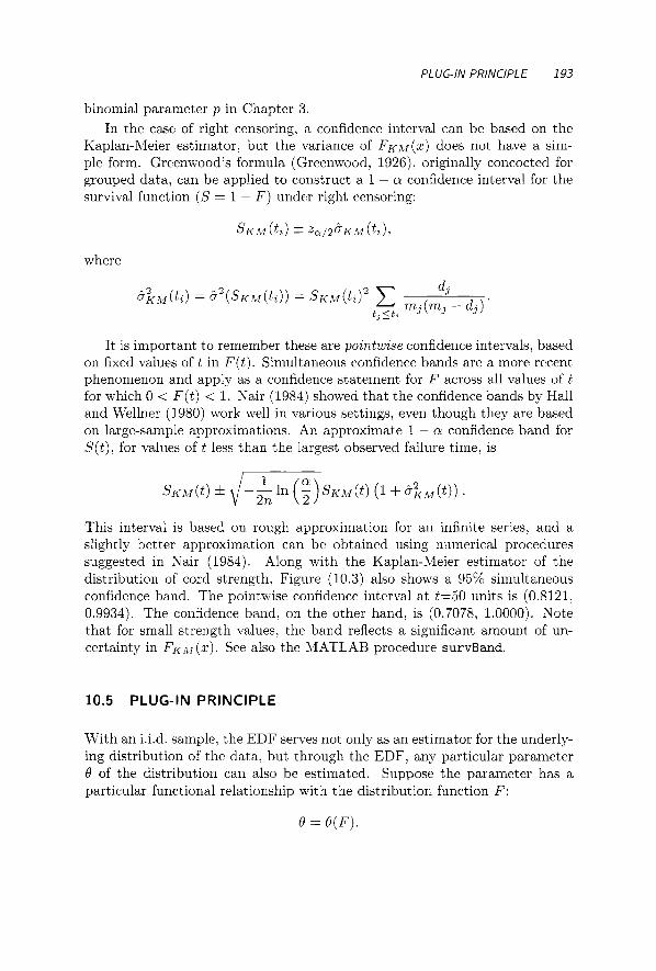
PLUG-/N PRlNClPLE 193
binomial parameter p in Chapter 3. In the case of right censoring, a confidence interval can be based on the
Kaplan-Meier estimator. but the variance of F ~ h f ( z ) does not have a sim- ple form. Greenwood’s formula (Greenwood, 1926), originally concocted for grouped data, can be applied to construct a 1 - cr confidence interval for the survival function ( S = 1 - F ) under right censoring:
where
It is important to remember these are pointwise confidence intervals. based on fixed values o f t in F ( t ) . Simultaneous confidence bands are a more recent phenomenon and apply as a confidence statement for F across all values o f t for which 0 < F ( t ) < 1. Kair (1984) showed that the confidence bands by Hall and Wellner (1980) work well in various settings, even though they are based on large-sample approximations. An approximate 1 - cr confidence band for S ( t ) . for values o f t less than the largest observed failure time, is
This interval is based on rough approximation for an infinite series, and a slightly better approximation can be obtained using numerical procedures suggested in Nair (1984). Along with the Kaplan-Meier estimator of the distribution of cord strength, Figure (10.3) also shows a 95% simultaneous confidence band. The pointwise confidence interval at t=50 units is (0.8121. 0.9934). The confidence band. on the other hand, is (0.7078, 1.0000). Note that for small strength values, the band reflects a significant amount of un- certainty in F K M ( z ) . See also the ICIATLAB procedure survBand.
10.5 PLUG-IN PRINCIPLE
With an i.i.d. sample. the EDF serves not only as an estimator for the underly- ing distribution of the data, but through the EDF, any particular parameter 8 of the distribution can also be estimated. Suppose the parameter has a particular functional relationship with the distribution function F :
0 = O(F).

194 ESTlMATlNG DlSTRlBUTlON FUNCTlONS
Examples are easy to construct. The population mean, for example, can be expressed
30
p = p ( F ) = 1 xdF(x) --oo
and variance is
As Fn is the sample analog to F , so .Q(Fn) can serve as a sample-based estimator for 6. This is the idea of the plug-in principle . The estimator for the population mean:
Obviously, the plug-in principle is not necessary for simply estimating the mean, but it is reassuring to see it produce a result that is consistent with standard estimating techniques.
Example 10.4 The quantile xp can be expressed as a function of F : xp = inf{x : s," d F ( z ) 5 1 - p } . The sample equivalent is the value gP = inf{z :
s," dFn(z) 5 1 - p } . If F is continuous, then we have xp = F - l ( p ) and Fn(eP) = p is solved uniquely. If F is discrete, eP is the smallest value of x for which
n
i=l
or, equivalently, the smallest order statistic x,, for which i / n 5 p , i.e.. (z + l ) / n > p . For example, with the flower data in Table 10.15, the me- dian waiting times are easily estimated as the smallest values (x) for which FKAJ(X) 5 1/2, which are 16 (for the male flowers) and 29 (for the female flowers).
If the data are not i.i.d.. the NPMLE F can be plugged in for F in Q ( F ) . This is a key selling point to the plug-in principle: it can be used to formulate estimators where we might have no set rule to estimate them. Depending on the sample, F might be the EDF or the Kaplan-Meier estimator. The plug-in technique is simple, and it will form a basis for estimating uncertainty using re-sampling techniques in Chapter 15.
Example 10.5 To find the average cord strength from the censored data, for example. it would be imprudent to merely average the data, as the censored observations represent a lower bound on the data, hence the true mean will be

SEMI-PARAMETRIC lNfERENCE 195
underestimated. By using the plug in principle, we will get a more accurate estimate; the code below estimates the mean cord strength as 54.1946 (see also the MATLAB m-file pluginmu. The sample mean, ignoring the censoring indicator, is 51.4438.
>> [cdfy svdata svcensor 1 = kmcdfsm(vdata,vcensor, ipresorted) ; >> if min(svdata)>O;
skm = 1-cdfy; %survival function
svdata2 = [O svdata’l; svdata3 = [svdata’ svdata(end1l ; dx = svdata3 - svdata2; mu-hat = skml *dx’;
cdfyl = CO, cdfy’l; cdfyi! = [cdfy’ 11; df = cdfy2 - cdfyl; svdatal = [svdata’, 01; mu-hat = svdatal *df’;
skml = [l, skm’l ;
else;
end ; >> mu-hat
ans =
154.1946
10.6 S E M I- PAR A M ET R I C I N F E R E N C E
The proportional hazards model for lifetime data relates two populations ac- cording to a common underlying hazard rate. Suppose ro(t ) is a baseline hazard rate, where r ( t ) = f ( t ) / ( l - F ( t ) ) . In reliability theory, r ( t ) is called the failure rate. For some covariate z that is observed along with the life- time, the positive function of Q(z) describes how the level of 5 can change the failure rate (and thus the lifetime distribution):
r ( t ; z) = ro(t)Q(z).
This is termed a semi-parametric model because ro(t) is usually left un- specified (and thus a candidate for nonparametric estimation) where as Q(5) is a known positive function, at least up to some possibly unknown parameters. Recall that the CDF is related to the failure rate as
r(u)du = R(u) = - In S(z). L where S(z) = 1 - F ( z ) is called the survivor function. R(t) is called the cumulative failure rate in reliability and life testing. In this case, So(t) is the

196 ESTIMATING DlSTRlBUTION FUNCTIONS
baseline survivor function, and relates to the lifetime affected by Q(z) as
S ( t ; z ) = S o ( t ) W
The most commonly used proportional hazards model used in survival analysis is called the Cox Model (named after Sir David Cox), which has the form
With this model, the (vector) parameter ,8 is left unspecified and must be estimated. Suppose the baseline hazard function of two different populations are related by proportional hazards as r l ( t ) = rO(t)X and rz(t) = ro(t)Q. Then if TI and Tz represent lifetimes from these two populations,
The probability does not depend at all on the underlying baseline hazard (or survivor) function. With this convenient set-up. nonparametric estimation of S( t ) is possible through maximizing the nonparametric likelihood. Suppose n possibly right-censored observations ( 2 1 , . . . , z,) from F = 1 - S are observed. Let & represent the number of observations at risk just before time 2,. Then, if S,=l indicates the lifetime was observed at xi,
In general. the likelihood must be solved numerically. For a thorough study of inference with a semi-parametric model. we suggest Statistical Models and Methods for Lifetime Data by Lawless. This area of research is paramount in survival analysis.
Related to the proportional hazard model, is the accelerated lafetime model used in engineering. In this case, the baseline survivor function So(t) can rep- resent the lifetime of a test product under usage conditions. In an accelerated life test, and additional stress is put on the test unit, such as high or low temperature, high voltage, high humidity, etc. This stress is characterized through the function @(z) and the survivor function of the stressed test item is
S( t ; z) = So(t@(.)).
Accelerated life testing is an important tool in product development, especially for electronics manufacturers who produce gadgets that are expected to last several years on test. By increasing the voltage in a particular way, as one example, the lifetimes can be shortened to hours. The key is how much faith

EMPIRICAL PROCESSES 197
the manufacturer has on the known acceleration function 9 ( z ) . In MATLAB, the Statistics Toolbox offers the routine coxphfit, which
computes Cox proportional hazards estimator for input data, much in the same way the kmcdf sm computes the Kaplan-Meier estimator.
10.7 EMPIRICAL PROCESSES
If we express the sample as X,(w), . . . . Xn(w), we note that F,(z) is both a function of z and w E a. From this. the EDF can be treated as a random process. The Glivenko-Cantelli Theorem from Chapter 3 states that the EDF F,(z) converges to F ( z ) (i) almost surely (as random variable, z fixed). and (ii) uniformly in z. (as a function of z with w fixed). This can be expressed as :
Let W ( z ) be a standard Brownian motion process. It is defined as a stochastic process for which W(0) = 0, W ( t ) N "(0, t ) , W ( t ) has independent increments, and the paths of W ( t ) are continuous. A Brownian Bridge is defined as B( t ) = W ( t ) - t W ( l ) , 0 5 t 5 1. Both ends of a Brownian Bridge, B(0) and B(l) , are tied to 0. and this property motivates the name. A Brownian motion W ( z ) has covariance function y( t , s) = t A s = rnin(t. s). This is because IE(N'(t)) = 0, Var(W(t)) = s, for s < t . Cov(W(t), W ( s ) ) =
@ov(W(s), (W(t) - W ( s ) ) + W ( s ) ) and W has independent increments. Define the random process B,(z) = &(F,(z) - F ( z ) ) . This process con-
verges to a Brownian Bridge Process, B ( z ) , in the sense that all finite dimen- sional distributions of B,(z) (defined by a selection of 5 1 , . . . , 2,) converge to the corresponding finite dimensional distribution of a Brownian Bridge B ( z ) .
Using this, one can show that a Brownian Bridge has mean zero and co- variance function y( t , s ) = t A s - t s . If s < t . y(s.t) = s(1 - t ) . For s < t , y(s , t ) = IE(W(s)-sW(l))(W(t)-tW(1)) = . . . = s - s t . BecausetheBrown- ian Bridge is a Gaussian process, it is uniquely determined by its second order properties. The covariance function y(t . s) for the process &(F,(t) - F ( t ) ) is:

198 ESTIMATING DISTRIBUTION FUNCTIONS
Proof:
11 IEy(t,s) = IE - C ( l ( X i < t ) - F ( t ) - C ( l ( X , < s) - F ( s ) [(i i ).(A j
1 n 1 n 1 n
= -IE(l(X1 < t ) - F( t ) ) ( l (X1 < s) - F ( s ) )
-IE [1(X1 < t A s ) - F ( t ) l ( X l < s ) - F ( s ) l ( X 1 < t ) + F ( t ) F ( s ) ] =
= - ( F ( t As) - F ( t ) F ( s ) ) .
This result is independent of F , as long as F is continuous, as the sample X I , . . . X , could be transformed to uniform: Y1 = F ( X 1 ) , . . . , Y, = F(X,) . Let G,(t) be the empirical distribution based on Yl, . . . , Y,. For the uniform distribution the covariance is ~ ( t , s ) = tAs - t s , which is exactly the correlation function of the Brownian Bridge. This leads to the following result:
Theorem 10.2 The random process f i ( F , ( z ) - F ( z ) ) converges in distri- bution to the Brownian Bridge process.
10.8 EMPIRICAL LIKELIHOOD
In Chapter 3 we defined the likelihood ratio based on the likelihood function L(Q) = n f(zi; Q ) , where X I , . . . X, were i.i.d. with density function f(z; 0). The likelihood ratio function
(10.5)
allows us to construct efficient tests and confidence intervals for the parameter 8. In this chapter we extend the likelihood ratio to nonparametric inference, although it is assumed that the research interest lies in some parameter 0 =
0 ( F ) . where F ( z ) is the unknown CDF. The likelihood ratio extends naturally to nonparametric estimation. If we
focus on the nonparametric likelihood from the beginning of this chapter. from an i.i.d. sample of X I . . . . X, generated from F ( z ) .
n n
i=l i=l

EMPlRlCAL LlKELlHOOD 199
The likelihood ratio corresponding to this would be R ( F ) = L ( F ) / L ( F , ) . where F, is the empirical distribution function. R ( F ) is called the empzrzcal lakelzhood ratao. In terms of F , this ratio doesn’t directly help us creating confidence intervals. All we know is that for any CDF F , R ( F ) 5 1 and reaches its maximum only for F = F,. This means we are considering only functions F that assign mass on the values X , = I,, a = 1,. . . .n. and R is reduced to function of n - 1 parameters R ( p 1 , . . . , p n - l ) where p , = d F ( z , ) and Cp, = 1.
It is more helpful to think of the problem in terms of an unknown pa- rameter of interest 6 = 6 ( F ) . Recall the plug-zn przncaple can be applied to estimate 6 with 8 = 6(Fn) . For example, with p = J z d F ( z ) was merely the sample mean, i.e. J z d F , ( s ) = 2 . We will focus on the mean as our first example to better understand the empirical likelihood.
Confidence Interval for the Mean. Suppose we have an i.i.d. sample X I , . . . . X , generated from an unknown distribution F ( z ) . In the case p ( F ) =
J s d F ( z ) , define the set C,(p) on p = (P I , . . . ,p,) as
The empirical likelihood associated with p maximizes L ( p ) over C,(p). The restriction Cp2s, = p is called the structural constraint. The empirical like- lihood ratio (ELR) is this empirical likelihood divided by the unconstrained NPMLE, which is just L ( l /n , . . . , l / n ) = n-n. If we can find a set of solutions to the empirical likelihood, Owen (1988) showed that
is approximately distributed x: if p is correctly specified. so a nonparametric confidence interval for p can be formed using the values of -2 log R ( p ) .
MATLAB software is available to help: e1m.m computes the empirical likelihood for a specific mean, allowing the user to iterate to make a curve for R ( p ) and. in the process. construct confidence intervals for p by solving R ( p ) = TO for specific values of ro. Computing R ( p ) is no simple matter; we can proceed with Lagrange multipliers to maximize Cpzz , subject to Cpz = 1 and C ln(np,) = ln(r0). The best numerical optimization methods are described in Chapter 2 of Owen (2001).
Example 10.6 Recall Exercise 6.2. Fuller et al. (1994) examined polished window strength data to estimate the lifetime for a glass airplane window. The units are ksi (or 1,000 psi). The MATLAB code below constructs the empirical likelihood for the mean glass strength, which is plotted in Figure

200 ESTIMATING DISTRIBUTION FUNCTIONS
10.4 (a). In this case, a 90% confidence interval for p is constructed by using the value of TO so that -2ln7-0 < x2(0.90) = 2.7055, or TO > 0.2585. The confidence interval is computed as (28.78 ksi, 33.02 ksi).
>>
>> >>
x = [18.83 20.8 21.657 23.03 23.23 24.05 24.321 25.5 25.52 25.8 . . . 26.69 26.77 26.78 27.05 27.67 29.9 31.11 33.2 33.73 33.76 33.89 . . . 34.76 35.75 35.91 36.98 37.08 37.09 39.58 44.045 45.29 45.381 1; n=size (x) ; i=i ; f o r mu=min(x):O.l:max(x) R-mu=elm(x, mu,zeros(l,l), 100, le-7, le-9, 0 ) ; ELR-mu(i)=R-mu; Mu(i)=mu; i=i+l;
end
-1
Fig. 10.4 (for different samples).
Empirical likelihood ratio as a function of (a) the mean and (b) the median
Owen's extension of Wilk's theorem for parametric likelihood ratios is valid for other functions of F , including the variance, quantiles and more. To construct R for the median, we need only change the structural constraint from Cpizi = ,LL to Cpi sign(zi - 2 0 . 5 0 ) = 0.
Confidence Interval for the Median. In general, computing R(z ) is difficult. For the case of estimating a population quantile, however, the opti- mizing becomes rather easy. For example, suppose that n1 observations out of n are less than the population median 20.50 and n2 = n - n1 observations are greater than 20.50. Under the constraint 20 .50 = 20.50 , the nonparametric likelihood estimator assigns mass (2nl)- ' to each observation less than Z0.50
and assigns mass (2nz ) - l to each observation to the right of 2 0 . 5 0 , leaving us

EXERClSES 201
with
Example 10.7 Figure 10.4(b). based on the MATLAB code below, shows the empirical likelihood for the median based on 30 randomly generated numbers from the exponential distribution (with p=l and 20.50 = - ln(0.5) = 0.6931). A 90% confidence interval for 20.50, again based on TO > 0.2585. is (0.3035, 0.9021).
For general problems, computing the empirical likelihood is no easy matter. and to really utilize the method fully, more advanced study is needed. This section provides a modest introduction to let you know what is possible using the empirical likelihood. Students interested in further pursuing this method are recommended to read Owen’s book.
10.9 EXERCISES
10.1. With an i.i.d. sample of n measurements. use the plug-in principle to derive an estimator for population variance.
10.2. Twelve people were interviewed and asked how many years they stayed at their first job. Three people are still employed at their first job and have been there for 1.5. 3.0 and 6.2 years. The others reported the following data for years at first job: 0.4, 0.9, 1.1. 1.9. 2.0, 3.3, 5.3, 5.8. 14.0. Using hand calculations. compute a noriparametric estimator for the distribution of T = time spent (in years) at first job. Verify your hand calculations using MATLAB. According to your estimator, what is the estimated probability that a person stays at their job for less than four years? Construct a 95% confidence interval for this estimate.
10.3. Using the estimator in Exercise 10.2. use the plug-in principle to com- pute the underlying mean number of years a person stays at their first job. Compare it to the faulty estimators based on using (a) only the noncensored items and (b) using the censored times but ignoring the censoring mechanism.
10.4. Consider Example 10.3, where we observe series-system lifetimes of a series system. We observe n different systems that are each made of kE

202 ESTlMATlNG DlSTRlBUTlON FUNCTIONS
identical components (i = 1, . . . ,n) with lifetime distribution F . The lifetime data is denoted ( 5 1 , . . . , z,) and are possibly right censored. Show that if we let rj = k j +. . . +in, the likelihood can be expressed as (10.5) and solve for the nonparametric maximum likelihood estimator.
10.5. Suppose we observe m different k-out-of-n systems and each system contains i.i.d. components (with distribution F ) , and the ith system contains ni components. Set up the nonparametric likelihood function for F based on the n system lifetimes (but do not solve the likelihood).
10.6. Go to the link below to download survival times for 87 people with lupus nephritis. They were followed for 15+ or more years after an initial renal biopsy. The duration variable indicates how long the patient had the disease before the biopsy; construct the Kaplan-Meier estimator for survival, ignoring the duration variable.
http://lib.stat.cmu.edu/datasets/lupus
10.7. Recall Exercise 6.3 based on 100 measurements of the speed of light in air. Use empirical likelihood to construct a 90% confidence interval for the mean and median.
http://www.itl.nist.gov/div898/strd/univ/data/Michelso.dat
10.8. Suppose the empirical likelihood ratio for the mean was equal to R ( p ) = p l ( 0 5 p 5 1) + (2 - p)1(1 5 p 5 2). Find a 95% confidence interval for p.
10.9. The Receiver Operating Characteristic (ROC) curve is a statistical tool to compare diagnostic tests. Suppose we have a sample of measurements (scores) X I , . . . , X , from a diseased population F ( z ) , and a sample of Yl, . . . , Y, from a healthy population G ( y ) . The healthy population has lower scores, so an observation is categorized as being diseased if it exceeds a given threshold value, e.g., if X > c. Then the rate of false- positive results would be P(Y > c) . The ROC curve is defined as the plot of R(p) = F(G- l (p ) ) . The ROC estimator can be computed using the plug-in principle:
= Fn(G;VP)).
A common test to see if the diagnostic test is effective is to see if R ( p ) remains well above 0.5 for 0 5 p 5 1. The Area Under the Curve (AUC) is defined as
1
AUC = .I R(p)dp.

REFERENCES 203
Show that AUC = P ( X 5 Y ) and show that by using the plug-in principle, the sample estimator of the AUC is equivalent to the Mann- Whitney two-sample test statistic.
REFERENCES
Brown, J. S. (1997), What It Means to Lead, Fast Company. 7. New York. Rlansueto Ventures. LLC.
Cox, D. R. (1972), "Regression Models and Life Tables.'' Journal of the Royal Statzstzcal Soczety (B), 34, 187-220.
Crowder. Ll. J.. Kimber, A. C., Smith. R. L., and Sweeting, T. J. (1991). Statzstzcal Analysts of Relzabzlzty Data. London, Chapman & Hall.
Fuller Jr.. E. R.. Frieman, S. W.. Quinn, J. B.. Quinn. G. D., and Carter, W. C. (1994). "Fracture Mechanics Approach to the Design of Glass Aircraft Windows: A Case Study", SPIE Proceedangs. Vol. 2286. (Society of Photo-Optical Instrumentation Engineers (SPIE) . Bellingham. WA) .
Greenwood, hl. (1926), "The Natural Duration of Cancer," in Reports on Publzc Health and Medzcal Subjects. 33. London: H. hl Stationery Office.
Hall, W. J.. and Wellner. J. A. (1980). -Confidence Bands for a Survival Curve." Bzometrzka, 67. 133-143
Kaplan, E. L.. and Neier. P. (1958). "Nonparametric Estimation from Incom- plete Observations." Journal of the Amerzcan Statzstzcal Assoczatzon. 53, 457-481.
Kiefer. J., and Wolfowitz, J. (1956). "Consistency of the hlaximum Likelihood Estimator in the Presence of Infinitely Many Incidental Parameters," Annals of Mathematzcal Statzstzcs. 27, 887-906.
Lawless. J. F. (1982), Statzstzcal Models and Methods for Lzfetzme Data, New York: Wiley.
Muenchow, G (1986). "Ecological Use of Failure Tirne Analysis." Ecology 67, 246250.
Kair, V. N. (1984). "Confidence Bands for Survival Functions with Censored Data. A Comparative Study," Technometrzcs, 26, 265-275.
Owen, A. B. (1988). "Empirical Likelihood Ratio Confidence Intervals for a Single Functional.'' Bzometrzka. 75, 237-249.
(1990). "Empirical Likelihood Confidence Regions," Annals of Statzs- tzcs. 18. 90-120
(2001), Empzrzcal Lzkelzhood. Boca Raton. FL: Chapman & Hall/CRC. Stigler, S. M. (1994), "Citations Patterns in the Journals of Statistics and
Probability." Statzstzcal Sczence. 9. 94-108.

This Page Intentionally Left Blank

Density Estimation
George McFly: Lorraine, my density has brought me to you. Lorraine Baines: What? George McFly: Oh. what I meant to say was. .. Lorraine Baines: Wait a minute, don’t I know you from somewhere? George McFly: Yes. Yes. I’m George, George McFly. I’m your density. I mean ... your destiny.
From the movie Back to the Future, 1985
Probability density estimation goes hand in hand with nonparametric estima- tion of the cumulative distribution function discussed in Chapter 10. There. we noted that the density function provides a better visual summary of how the random variable is distributed across its support. Symmetry, skewness. disperseness and unimodality are just a few of the properties that are ascer- tained when we visually scrutinize a probability density plot.
Recall. for continuous i.i.d. data. the empzrzcal denszty f unc t zon places probability mass 1/n on each of the observations. While the plot of the empirical dzstrzbutzon function (EDF) emulates the underlying distribution function. for continuous distributions the empirical density function takes no shape beside the changing frequency of discrete jumps of 1/n across the domain of the underlying distribution - see Figure 11.2(a).
205

206 DENSlTY ESTlMATlON
Fig. 11.1 Playfair’s 1786 bar chart of wheat prices in England
11.1 HISTOGRAM
The histogram provides a quick picture of the underlying density by weighting fixed intervals according the their relative frequency in the data. Pearson (1895) coined the term for this empirical plot of the data, but its history goes as far back as the 18th century. William Playfair (1786) is credited with the first appearance of a bar chart (see Figure 11.1) that plotted the price of wheat in England through the 17th and 18th centuries.
In MATLAB, the procedure hist (x) will create a histogram with ten bins using the input vector x. Figure 11.2 shows (a) the empirical density function where vertical bars represent Dirac’s point masses at the observations, and (b) a 10-bin histogram for a set of 30 generated N(0,l) random variables. Obviously, by aggregating observations within the disjoint intervals, we get a better, smoother visual construction of the frequency distribution of the sample.
>> x = rand_nor(O,l,30,1); >> hist(x) >> histfit(x,1000)
The histogram represents a rudimentary smoothing operation that pro- vides the user a way of visualizing the true empirical density of the sample. Still, this simple plot is primitive, and depends on the subjective choices the user makes for bin widths and number of bins. With larger data sets, we can increase the number of bins while still keeping average bin frequency at a reasonable number. say 5 or more. If the underlying data are continuous, the histogram appears less discrete as the sample size (and number of bins) grow, but with smaller samples, the graph of binned frequency counts will not pick up the nuances of the underlying distribution.

KERNEL AND BANDWIDTH 207
04-
0 3 -
0 2 -
O i -
-2 - 1 5 -1 -05 0 0 5 l
(a)
1 5
1 1 2 2 5
Fig. 11.2 Empirical "density" (a) and histogram (b) for 30 normal N(0,l) variables.
The MATLAB function h i s t f it (x,n) plots a histogram with n bins along with the best fitting normal density curve. Figure 11.3 shows how the appear- ance of continuity changes as the histogram becomes more refined (with more bins of smaller bin width). Of course, we do not have such luxury with smaller or medium sized data sets; and are more likely left to ponder the question of underlying normality with a sample of size 30, as in Figure 11.2(b).
>> x = rand_nor(O,1,5000,1); >> histfit(x,lO) >> histf it (x, 1000)
If you have no scruples, the histogram provides for you many opportunities to mislead your audience, as you can make the distribution of the data appear differently by choosing your own bin widths centered at a set of points arbi- trarily left to your own choosing. If you are completely untrustworthy, you might even consider making bins of unequal length. That is sure to support a conjectured but otherwise unsupportable thesis with your data, and might jump-start a promising career for you in politics.
11.2 KERNEL AND BANDWIDTH
The idea of the density estimator is to spread out the weight of a single observation in a plot of the empirical density function. The histogram, then, is the picture of a density estimator that spreads the probability mass of each sample item uniformly throughout the interval (i.e.. bin) it is observed in.

208 DENSlTY ESTlMATlON
Fig. 11.3 Histograms with normal fit of 5000 generated variables using (a) 10 bins and (b) 50 bins.
Note that the observations are in no way expected to be uniformly spread out within any particular interval, so the mass is not spread equally around the observation unless it happens to fall exactly in the center of the interval.
In this chapter, we focus on the kernel density estimator that more fairly spreads out the probability mass of each observation, not arbitrarily in a fixed interval, but smoothly around the observation, typically in a symmetric way. With a sample XI, . . . , X,, we write the density estimator
(11.1)
for X , = x,. i = 1,. . . , n. The kernel function K represents how the probabil- ity mass is assigned, so for the histogram. it is just a constant in any particu- lar interval. The smoothing function h, is a positive sequence of bandwidths analogous to the bin width in a histogram.
The kernel function K has five important properties -
1. K ( x ) 2 0 vx 2 . K ( x ) = K ( - x ) for IC > 0 3. J K ( u ) d u = 1 4. JuK(u)du = 0 5 . JuZK(u)du = 0: < m.

KERNEL AND BANDWlDTH 209
Fig. 11.4 tions.
(a) Normal, (b) Triangular, (c) Box, and (d) Epanechnickov kernel func-
Figure 11.4 shows four basic kernel functions:
1. Normal (or Gaussian) kernel K ( z ) = $(x),
2. Triangular kernel K ( J : ) = C-"C - 1x1) 1(-c < z < c), c > 0.
3. Epanechnickov kernel (described below).
4. Box kernel, K ( z ) = 1(-c < J: < c)/(2c), c > 0.
While K controls the shape. h, controls the spread of the kernel. The accuracy of a density estimator can be evaluated using the mean integrated squared error, defined as
MISE = E ( / ( f ( z ) - f(~))~dz)
= /Bias'(f(z))dz + Var(f(z))dz. (11.2) s To find a density estimator that minimizes the MISE under the five mentioned constraints, we also will assume that f ( x ) is continuous (and twice differen- tiable), h, -+ 0 and nh, + cc as n 4 m. Under these conditions it can be

210 DENSITY ESTIMATION
shown that
Bias(f(x)) = &f”(x ) + O(h:) and 2
(11.3)
where R(g) = J g(u)2du.
We determine (and minimize) the MISE by our choice of h,. From the equations in (11.3), we see that there is a tradeoff. Choosing h, to reduce bias will increase the variance, and vice versa. The choice of bandwidth is important in the construction of f(x). If h is chosen to be small, the subtle nuances in the main part of the density will be highlighted, but the tail of the distribution will be unseemly bumpy. If h is chosen large. the tails of the distribution are better handled, but we fail to see important characteristics in the middle quartiles of the data.
By substituting in the bias and variance in the formula for (11.2), we minimize MISE with
At this point, we can still choose K ( x ) and insert a “representative” density for f(x) to solve for the bandwidth. Epanechnickov (1969) showed that. upon substituting in f ( z ) = q5(x)? the kernel that minimizes MISE is
The resulting bandwidth becomes h: FZ 1.068n-’/’, where 8 is the sample standard deviation. This choice relies on the approximation of 0 for f(x). Alternative approaches. including cross-validation, lead to slightly different answers.
Adaptive kernels were derived to alleviate this problem. If we use a more general smoothing function tied to the density at x3. we could generalize the density estimator as
(11.4)
This is an advanced topic in density estimation, and we will not further pur- sue learning more about optimal estimators based on adaptive kernels here. We will also leave out details about estimator limit properties, and instead point out that if h, is a decreasing function of n, under some mild regularity
conditions, lf(x) -f(x)I 5 0. For details and more advanced topics in density

KERNEL AND BANDWIDTH 211
fig. 11.5 Density estimation for sample of size n=7 using various kernels: (all) Nor- mal, (a) Box, (b) Triangle, (c) Epanechnikov.
-1 0 4
0 35
Fig. 11.6 Density estimation for sample of size n = 7 using various bandwidths.
estimation, see Silverman (1986) and Efromovich (1999). The (univariate) density estimator from T\;I ATLAB. called
ksdensity(data1.
is illustrated in Figure 11.5 using a sample of seven observations. The default estimate is based on a normal kernel: to use another kernel, just enter 'box', 'triangle', or 'epanechnikov' (see code below). Figure 11.5 shows how the nor- mal kernel compares to the (a) box. ( 2 ) triangle and (c) epanechnikov kernels. Figure 11.6 shows the density estimator using the same data based on the normal kernel. but using three different bandwidths. Note the optimal band- width (0.7449) can be found by allowing a third argument in the ksdensity output.
>> datal=[11,12,12.2,12.3,13,13.7,18];

212 DENSlTY ESTlMATlON
>> data2=[50,21,25.5,40.0,41,47.6,39]; >> [fl,xl]=ksdensity(datal,’kernel’, ’box’); >> plot(xl,fl,’-k’) >> hold on >> [f2,~2,band]=ksdensity(datal) ; >> plot(x2,f2,’:kJ) >> band
band = 0.7449
>> [fl,xl]=ksdensity(datal,’width’,2); >> plot(xl,fl, ’--k’) >> hold on >> [fl,xl]=ksdensity(datal,’width’,l); >> plot(xl,fl,’-k’) >> [fl,xll=ksdensity(datal, ’width’, .5) ; >> plot(xl,fl,’:k’)
Censoring. The MATLAB function ksdensity also handles right-censored data by adding an optional vector designating censoring. Although we will not study the details about the way density estimators handle this problem. censored observations are treated in a way similar to nonparametric max- imum likelihood, with the weight assigned to the censored observation xc being distributed proportionally to non-censored observations xt 2 x, (see the Kaplan-Meier estimator in Chapter 10). General weighting can also be included in the density estimation for ksdensity with an optional vector of weights.
Example 11.1 Radiation Measurements. In some situations, the exper- imenter might prefer to subjectively decide on a proper bandwidth instead of the objective choice of bandwidth that minimizes MISE. If outliers and subtle changes in the probability distribution are crucial in the model, a more jagged density estimator (with a smaller bandwidth) might be preferred to the optimal one. In Davies and Gather (1993), 2001 radiation measurements were taken from a balloon at a height of 100 feet. Outliers occur when the balloon rotates, causing the balloon‘s ropes to block direct radiation from the sun to the measuring device. Figure 11.7 shows two density estimates of the raw data. one based on a narrow bandwidth and the other more smooth density based on a bandwidth 10 times larger (0.01 to 0.1). Both densities are based upon a normal (Gaussian) kernel. While the more jagged estima- tor does show the mode and skew of the density as clearly as the smoother estimator, outliers are more easily discerned.
>> T=load( ’balloondata.txt’); >> ~ 1 = ~ ( : , 1 ) ; T2=T(:,2); >> [fl,xl]=ksdensity(Tl, ’width’, . O i l ;

EXERCISES 213
Fig. 11.7 Density estimation for 2001 radiation measurements using bandwidths band = 0.5 and band=0.05.
>> plot(xl,fl,’-k’) >> hold on >> [f2,~2]=ksdensity(TI, ’width’, .I) ; >> plot(x2,f2,’:k’)
11.2.1 Bivariate Density Estimators
To plot density estimators for bivariate data, a three-dimensional plot can be constructed using MATLAB function k d f f t 2 , noting that both x and y, the vectors designating plotting points for the density, must be of the same size.
In Figure 11.8; (univariate) density estimates are plotted for the seven observations [ d a t a l , data21. In Figure 11.9, k d f f t 2 is used to produce a two-dimensional density plot for the seven bivariate observations (coupled together).
11.3 EXERCISES
11.1. Which of the following serve as kernel functions for a density estimator? Prove your assertion one way or the other.
a. K ( z ) = I(-1 < J: < 1) /2 ;
b. K ( z ) = l ( 0 < J: < 1).

214 DENSITY ESTIMATION
I
0 35
Fig. 11.8 estimator for second variable.
(a) Univariate density estimator for first variable; (b) Univariate density
c. K ( z ) = l /z,
d. K ( z ) = $(2z + 1)(1 - 2z) 1(-i < z < i), e. K ( z ) = 0.75(1 - z2) 1(-1 < z < 1)
11.2. With a data set of 12, 15, 16, 20, estimate p* = P(observation is less than 15) using a density estimator based on a normal (Gaussian) ker- nel with h, = m. Use hand calculations instead of the MATLAB function.
11.3. Generate 12 observations from a mixture distribution, where half of the observations are from n/(O, 1) and the other half are from n/(1,0.64). Use the MATLAB function ksdensity to create a density estimator. Change bandwidth to see its effect on the estimator. Repeat this pro- cedure using 24 observations instead of 12.
11.4. Suppose you have chosen kernel function K ( z ) and smoothing function h, to construct your density estimator, where -co < K ( z ) < co. What should you do if you encounter a right censored observation? For exam- ple. suppose the right-censored observation is ranked m lowest out of n, m s n - 1 .
11.5. Recall Exercise 6.3 based on 100 measurements of the speed of light in air. In that chapter we tested the data for normality. Use the same data to construct a density estimator that you feel gives the best visual display of the information provided by the data. What parameters did you choose? The data can be downloaded from
http://www.itl.nist.gov/div898/strd/univ/data/Michelso.dat

REFERENCES 215
Fig. 11.9 Bivariate Density estimation for sample of size n = 7 using bandwidth =
[2,21.
11.6. Go back to Exercise 10.6. where a link is provided to download right- censored survival times for 87 people with lupus nephritis. Construct a den&ity estimator for the survival, ignoring the duration variable.
http://lib.stat.cmu.edu/datasets/lupus
REFERENCES
Davies, L., and Gather, U. (1993) , ‘.The Identification of Multiple Outliers” (discussion paper), Journal of the Amer ican Statistical Association, 88,
Efromovich, S . (1999) , Nonparametric Curve Est imation: Methods, Theory and Applications, New York: Springer Verlag.
Epanechnikov, V. A. (1969) , “Nonparametric Estimation of a hlultivariate Probability Density,“ Theory of Probability and i ts Applications, 14, 153- 158.
Pearson, K. (1895) , Contributions t o the Mathematical Theory of Evolution II, Philosophical Transactions of the Royal Society of London (A) ,186,
782-792.

216 DENSlTY ESTlMATlON
343-414 Playfair, W. (1786), Commercial and Political Atlas: Representing, b y Copper-
Plate Charts, the Progress of the Commerce, Revenues, Expenditure, and Debts of England, during the Whole of the Eighteenth Century. London: Corry.
Silverman, B. (1986), Density Estimation for Statistics and Data Analysis, New York: Chapman & Hall.

12 Beyond Linear
Regress i o n
Essentially, all models are wrong, but some models are useful.
George Box, from Empirical Model-Building and Response Surfaces
Statistical methods using linear regression are based on the assumptions that errors, and hence the regression responses, are normally distributed. Variable transformations increase the scope and applicability of linear regres- sion toward real applications. but many modeling problems cannot fit in the confines of these model assumptions.
In some cases, the methods for linear regression are robust to minor vi- olations of these assumptions. This has been shown in diagnostic methods and simulation. In examples where the assumptions are more seriously vio- lated, however. estimation and prediction based on i he regression model are biased. Some reszduals (measured difference between the response and the model's estimate of the response) can be overly large in this case, and wield a large influence on the estimated model. The observations associated with large residuals are called outliers. which cause error variances to inflate and reduce the power of the inferences made.
In other applications. parametric regression techniques are inadequate in capturing the true relationship between the response and the set of predictors. General "curve fitting" techniques for such data problems are introduced in the next chapter. where the model of the regression is unspecified and not necessarily linear.
In this chapter, we look at simple alternatiyes to basic least-squares re-
217

218 BEYOND LlNEAR REGRESSlON
gression. These estimators are constructed to be less sensitive to the outliers that can affect regular regression estimators. Robust regression estimators are made specifically for this purpose. Nonparametric or rank regression relies more on the order relations in the paired data rather than the actual data measurements, and isotonic regression represents a nonparametric regression model with simple constraints built in, such as the response being monotone with respect to one or more inputs. Finally, we overview generalized linear models which although parametric, encompass some nonparametric methods, such as contingency tables, for example.
12.1 LEAST SQUARES REGRESSION
Before we introduce the less-familiar tools of nonparametric regression, we will first review basic linear regression that is taught in introductory statistics courses. Ordinary least-squares regression is synonymous with parametric re- gression only because of the way the errors in the model are treated. In the simple linear regression case, we observe n independent pairs ( X i , x), where the linear regression of Y on X is the conditional expectation IE(Y1X). A char- acterizing property of normally distributed X and Y is that the conditional expectation is linear, that is, IE(Y1X) = PO + PIX.
errors xi(x - g ) 2 = Ci(Y, - [PO + P1Xi])2 with respect to the parameters Standard least squares regression estimates are based on minimizing squared
and PO. The least squares solutions are
C;=l(xi - X ) ( K - Y ) c;=l(Xz - X ) 2
- (Xzyz - n X Y ) En 2=1 X ? - n X 2 '
P1 =
-
a 0 = Y - p J
(12.1)
(12.2)
This solution is familiar from elementary parametric regression. In fact. (&.a1) are the MLEs of (PO. P I ) in the case the errors are normally dis- tributed. But with the minimized least squares approach (treating the sum of squares as a "loss function"). no such assumptions were needed, so the model is essentially nonparametric. However, in ordinary regression. the distribu- tional properties of fro and p1 that are used in constructing tests of hypothesis and confidence intervals are pinned to assuming these errors are homogenous and normal.

RANK REGRESSION 219
12.2 RANK REGRESSION
The truest nonparametric method for modeling bivariate data is Spearman's correlation coefficient which has no specified model (between X and Y) and no assumed distributions on the errors. Regression methods, by their nature. require additional model assumptions to relate a random variable X to Y via a function for the regression of JE(Y/X) . The technique discussed here is nonparametric except for the chosen regression model; error distributions are left to be arbitrary. Here we assume the linear model
y, = Po + &Xi, 2 = 1,. . . , 12
is appropriate and. using the squared errors as a loss function, we compute $0 and f i 1 as in (12.2) and (12.1) as the least-squares solution.
Suppose we are interested in testing HO that the population slope is equal to against the three possible alternatives, HI : 01 > PIO, H I : PI < PIO, H I : /31 # @lo. Recall that in standard least-squares regression, the Pearson coefficient of linear correlation (6) between the X s and Y s is connected to .01
via
+Q,. &FGiF Jm'
To test the hypothesis about the slope. first calculate U, = Y, -/3loX,, and find the Spearman coefficient of rank correlation j3 between the X,s and the U,s. For the case in which Plo = 0. this is no more than the standard Spear- man correlation statistic. In any case, under the assumption of independence, (b - p ) m - N(O.1) and the tests against alternatives H1 are
Alternative p-value
where 2 - N(O.1). The table represents a simple nonparametric regression test based only on Spearman's correlation statistic.
Example 12.1 Active Learning. Kvam (2000) examined the effect of ac- tive learning methods on student retention by examining students of an in- troductory statistics course eight months after the course finished. For a class taught using an emphasis on active learning techniques, scores were compared to equivalent final exam scores.
Exam 1 14 15 18 16 17 12 17 15 17 14 17 13 15 18 14 Exam2 14 10 11 8 17 9 11 13 12 13 14 11 11 15 9

220 BEYOND LlNEAR REGRESSlON
Scores for the first (z-axis) and second (y-axis) exam scores are plotted in Figure 12.l(a) for 15 active-learning students. In Figure 12.1(b), the solid line represents the computed Spearman correlation coefficient for X i and Ui = Y , - @loxi with PI0 varying from -1 to 1. The dashed line is the pvalue corresponding to the test HI : p1 # @lo. For the hypothesis Ho : P1 2 0 versus H1 : p1 < 0, the p-value is about 0.12 (the p-value for the two-sided test, from the graph, is about 0.24).
Note that at plo = 0.498, 6 is zero, and at /?lo = 0, j3 = 0.387. The pvalue is highest at plo = 0.5 and less than 0.05 for all values of Plo less than - 0.332.
>> n0=1000; >> S=load(’activelearning.txt’); >> tradl=S(:,l); trad2=S(:,2); >> acti=S(:,3); act2=S(:,4); >> trad= [tradl trad21 ; act= [actl act21 ; >> r=zeros (no, 1) ; p=zeros (no, 1) ; b=zeros(nO, 1) ;
>> for i=l:nO b(i)=(i- (n0/2) /(n0/2) ; [rO z0 PO] =spear(actl, act2-b(i) *act11 ; r (i) =rO ; p (i)=pO ; end
>> stairs(b,p,’:k’) >> hold on >> stairs(b,r,’-k’)
12 14 16 18 Test 1
I
-021
-0.4 I -1 -0.5 0 0.5 1
Slwe Parameter
Fig. 12.1 (a) Plot of test #1 scores (during term) and test # 2 scores (8 months after). (b) Plot of Spearman correlation coefficient (solid) and corresponding p-value (dot ted) for nonparametric test of slope for -1 5 P ~ o 5 1.

ROBUST REGRESSlON 221
12.2.1
Among n bivariate observations. there are (z) different pairs ( X t , y Z ) and ( X , , q ) , i # j . Foreachpair(X,,Y,)and(X3.q),1<-i<j<-nwefindthe corresponding slope
Sen-Theil Estimator of Regression Slope
Y3 - Yz - x, - Xi'
s . . -
Compared to ordinary least-squares regression, a more robust estimator of the slope parameter is
- p1 = median{&,. 1 <- i < j 5 n}.
Corresponding to the least-squares estimate, let
60 = median{Y} - $Imedian{X}.
Example 12.2 If we take n = 20 integers (1,. . . ,20} as our set of predictors X I . . . . ~ Xzo, let Y be 2X + E where E is a standard normal variable. Next. we change both Y1 and Y ~ o to be outliers with value 20 and compare the ordinary least squares regression with the more robust nonparainetric method in Figure 12.2.
-7 45,
40
35 \ 30 ) 251
I
15-
10-
5 -
2o r
~~
0 5 10 15 20 25
Fig. 12.2 Regression: Least squares (dotted) and nonparametric (solid).
12.3 ROBUST REGRESSION
"Robust" estimators are ones that retain desired statistical properties even when the assumptions about the data are slightly off. Robust linear regres-

222 BEYOND LlNEAR REGRESSlON
sion represents a modeling alternative to regular linear regression in the case the assumptions about the error distributions are potentially invalid. In the simple linear case, we observe n independent pairs ( X % , E), where the linear regression of Y on X is the conditional expectation IE(Y1X) = PO + P I X .
For rank regression, the estimator of the regression slope is considered to be robust because no single observation (or small group of observations) will have an significant influence on estimated model; the regression slope picks out the median slope out of the (;) different pairings of data points.
One way of measuring robustness is the regression’s breakdown point, which is the proportion of bad data needed to affect the regression adversely. For example, the sample mean has a breakdown point of 0, because a single obser- vation can change it by an arbitrary amount. On the other hand, the sample median has a breakdown point of 50 percent. Analogous to this, ordinary least squares regression has a breakdown point of 0, while some of the robust techniques mentioned here (e.g., least-trimmed squares) have a breakdown point of 50 percent.
There is a big universe of robust estimation. We only briefly introduce some robust regression techniques here. and no formulations or derivations are given. A student who is interested in learning more should read an intro- ductory textbook on the subject, such as Robust Statwtics by Huber (1981).
12.3.1 Least Absolute Residuals Regression
By squaring the error as a measure of discrepancy, the least-squares regression is more influenced by outliers than a model based on. for example. absolute deviation errors: C, lY, - 21, which is called Least Absolute Residuals Re- gression. By minimizing errors with a loss function that is more “forgiving” to large deviations, this method is less influenced by these outliers. In place of least-squares techniques, regression coefficients are found from linear pro- gramming.
12.3.2 Huber Estimate
The concept of robust regression is based on a more general class of estimates (30,bI) that minimize the function
2 V ( Y , - R) CT
2 = 1
where u is a loss function and 0 is a scale factor. If $(x) = x2, we have regular least-squares regression, and if +(x) = 1x1, we have least absolute residuals

ROBUST REGRESSION 223
regression. A general loss function introduced by Huber (1975) is
Depending on the chosen value of c > 0. G(z) uses squared-error loss for small errors, but the loss function flattens out for larger errors.
12.3.3 Least Trimmed Squares Regression
Least Trimmed Squares (LTS) is another robust regression technique proposed by Rousseeuw (1985) as a robust alternative to ordinary least squares regres- sion. Within the context of the linear model y, = P’x,, i = I, . . . . n, the LTS estimator is represented by the value of that minimizes Cz=l T, n. Here. xt is a pxl vector and T , is the z t h order statistic from the squared residuals T, = (y, - P’X,)~ and h is a trimming constant (n /2 5 h 5 n) chosen so that the largest n - h residuals do not affect the model estimate. Rousseeuw and Leroy (1987) showed that the LTS estimator has its highest level of robustness when h = [n/2] + [ ( p + l ) / 2 ] . While choosing h to be low leads to a more robust estimator, there is a tradeoff of robustness for efficiency.
h
12.3.4 Weighted Least Squares Regression
For some data, one can improve model fit by including a scale factor (weight) in the deviation function. Weighted least squares minimizes
n
2 = 1
where w, are weights that determine how much influence each response will have on the final regression. With the weights in the model, we estimate /3 in the linear model with
9 = (x’wx)-l x ’ w y ,
where X is the design matrix made up of the vectors zz, y is the response vector. and W is a diagonal matrix of the weights w1,. . . . w,. This can be especially helpful if the responses seem not to have constant variances. Weights that counter the effect of heteroskedasticity, such as

224 BEYOND LINEAR REGRESSION
work well if your data contain a lot of replicates; here m is the number of replicates at yz. To compute this in MATLAB, the function l s c o v computes least-squares estimates with known covariance; for example, the output of
lscov(A,B,W)
returns the weighted least squares solution to the linear system A X = B with diagonal weight matrix X.
12.3.5 Least Median Squares Regression
The least median of squares (LMS) regression finds the line through the data that minimizes the median (rather than the mean) of the squares of the errors. While the LMS method is proven to be robust, it cannot be easily solved like a weighted least-squares problem. The solution must be solved by searching in the space of possible estimates generated from the data, which is usually too large to do analytically. Instead, randomly chosen subsets of the data are chosen so that an approximate solution can be computed without too much trouble. The MATLAB function
lmsreg(y, X>
computes the LMS for small or medium sized data sets.
Example 12.3 Star Data. Data from Rousseeuw and Leroy (1987), p. 27, Table 3, are given in all panels of Figure 12.3 as a scatterplot of temperature versus light intensity for 47 stars. The first variable is the logarithm of the effective temperature at the surface of the star (Te) and the second one is the logarithm of its light intensity (LILO). In sequence, the four panels in Figure 12.3 show plots of the bivariate data with fitted regressions based on (a) Least Squares, (b) Least Absolute Residuals. (c) Huber Loss & Least Trimmed Squares, and (d) Least Median Squares. Observations far away from most of the other observations are called leverage points; in this example, only the Least Median Squares approach works well because of the effect of the leverage points.
>> stars = load(’stars.txt’); n = size(stars,l); >> x = Cones(n,i) stars(:,2)1; y = stars(:,3); >> bols = X\y; [ignore,idx] = sort(stars(:,2)); >> plot(stars(:,2),stars(:,3),’o’,stars(idx,2), . . .
X(idx,:)+bols,’-.’ )
legend(’Data’,’OLS’) >> % >> % Least Absolute Deviation >> blad = medianregress(stars(: ,2) ,stars(: , 3 ) ) ; >> plot(stars(:,2),stars(:,3),’oJ,stars(idx,2), . . .
X(idx,:)*bols,’-.’,stars(idx,2),X(idx,:)*blad,’-.’) legend(’Data’,’OLS’,’LAD’);

ROBUST REGRESSlON 225
651 , ,
351 ' ' ' ' ' I 3 4 36 3 8 4 4 2 4 4 4 6 4 6 5
35.- 34 36 3 8 4 4 2 4 4 4 6 4 0 5
- 1 0 I
3 . 5 - - , ' ' I 3 4 36 36 4 4 2 4 4 4 6 4 8 5
Fig. 12.3 Estimation and Least Trimmed Squares, (d) Least Median Squares.
Star data with (a) OLS Regression, (b) Least Absolute Deviation. (c) Huber
>> % >> % Huber Estimation >> k = 1.345; % tuning parameters in Huber's weight function >> wgtfun = O(e) (k*(abs(e)>k)-abs(e) .*(abs(e)>k)) ./abs(e)+l; >> % Huber's weight function >> wgt = rand(length(y),l); >> bO = lscov(X,y,wgt); >> res = y - X*bO; >> res = res/mad(res)/0.6745; % Standardized Residua1:s >> rn = 30; >> for i=l:m
% Initial Weights
% Raw Residuals
wgt = wgtfun(res); % Compute the weighted estimate using these weights bhuber = lscov(X,y,wgt); if all((bhuber-bO)<.Ol*bO)% Stop with convergence
else return;
res = y - X+bhuber;

226 BEYOND LINEAR REGRESSlON
res = res/mad(res)/0.6745; end
end >> plot(stars(:,2),stars(:,3),’o’,stars(idx,2),X(idx,:).
*bols,’-.’, stars(idx,2),X(idx,:)*blad,’-x’, . . . stars(idx,2),X(idx,:)*bhuber,’-s’) legend(’Data’,’OLS’,’LAD’,’Huber’);
>> % >> % Least Trimmed Squares >> blts = lts(stars(: , 2 ) , y ) ; >> plot(stars(:,2),stars(:,3),’oJ,stars(idx,2),X(idx,:).
*bols,’-.’, stars(idx,2),X(idx,:)*blad,’-x’, . . . stars(idx,2),X(idx,:)*bhuber,’-s’, stars(idx,2), . . . X(idx,:)*blad,’-+’) legend(’Data’,’OLS’,’LAD’,’Huber’,’LTS’);
>> % >> % Least Median Squares >> [LMSout,blms,Rsq]=LMSreg(y,stars(:,2)); >> plot(stars(:,2),stars(: ,3),’0’,stars(idx,Z),X(idx, : ) .
*bols,’-.’,stars(idx,2),X(idx,:)*blad,’-x’,... stars(idx,2), X(idx,:)*bhuber,’-s’,stars(idx,2), . . . X(idx,:)+blad,’-+’, stars(idx,Z),X(idx,:)*blms,’-d’) legend(’Data’,’OLS’,’LAD’,’Huber’,’LTS’,’LMS’);
Example 12.4 Anscombe’s Four Regressions. A celebrated example of the role of residual analysis and statistical graphics in statistical modeling was created by Anscombe (1973). He constructed four different data sets ( X z . x), i = 1.. . . ,11 that share the same descriptive statistics (X, Y,bo. 81, M S E , R2. F ) necessary to establish linear regression fit Y = bo + & X . The following statistics are common for the four data sets:
Sample size N 11 Mean of X ( X ) 9 Mean of Y (Y ) 7.5 Intercept 3 Slope (A ) 0.5 Estimator of CT, (s) 1.2366 Correlation T X , ~ 0.816
From inspection, one can ascertain that a linear model is appropriate for Data Set 1. but the scatter plots and residual analysis suggest that the Data Sets 2-4 are not amenable to linear modeling. Plotted with the data are the lines for least-square fit (dotted) and rank regression (solid line). See Exercise 12.1 for further examination of the three regression archetypes.

lSOTONlC REGRESSlON 227
X Y
Data Set 1
10 8 13 9 11 14 6 4 12 7 5 8.04 6.95 7.58 8.81 8.33 9.96 7.24 4.26 10.84 4.82 5.68
X Y
Data Set 2
10 8 13 9 11 14 6 4 12 7 5 9.14 8.14 8.74 8.77 9.26 8.10 6.13 3.10 9.13 7.26 4.74
X Y
12.4 ISOTONIC REGRESSION
Data Set 3
10 8 13 9 11 14 6 4 12 7 5 7.46 6.77 12.74 7.11 7.81 8.84 6.08 5.39 8.15 6.42 5.73
In this section we consider bivariate data that satisfy an order or restriction in functional form. For example, if Y is known to be a decreasing function of X , a simple linear regression need only consider values of the slope parameter /31 < 0. If we have no linear model, however: there is nothing in the empirical bivariate model to ensure such a constraint is satisfied. Isotonic regression considers a restricted class of estimators without the use of an explicit regres- sion model.
Consider the dental study data in Table 12.16, which was used to illustrate isotonic regression by Robertson, Wright, and Dykstra (1988). The data are originally from a study of dental growth measurements of the distance (mm) from the center of the pituitary gland to the pterygoniaxillary fissure (referring to the bone in the lower jaw) for 11 girls between the age of 8 and 14. It is assumed that PF increases with age. so the regression of PF on age is nondecreasing. But it is also assumed that the relationship between PF and age is not necessarily linear. The means (or medians, for that matter) are not strictly increasing in the PF data. Least squares regression does yield an increasing function for PF: Y = 0.065X + 21.89. but the function is nearly flat and not altogether well-suited to the data.
For an isotonic regression, we impose some order of the response as a function of the regressors.
Definition 12.1 If the regressors have a simple order x1 5 . . . 5 x,, a function f is isotonic with respect to x if f ( x 1 ) 5; . . . 5 f ( x , ) . For our purposes, isotonic wall be synonymous with mon,otonic. For same function g of X , we call the function g l ; an isotonic regression of g with weights w if and
Y
Data Set 4
6.58 5.76 7.71 8.84 8.47 7.04 5.25 12.50 5.56 7.91 6.89 X 8 8 8 8 8 8 8 19 8 8 8

228 BEYOND LlNEAR REGRESSlON
14 I
t /
14, I
4; 6 b 10 12 14 16 1s 20
(4
Fig. 12.4 Anscombe’s regressions: LS and Robust.
only if g* i s i so ton ic (i .e. , re tains the necessary order) and m i n i m i z e s
n
(12.3)
in the class of all isotonic f u n c t i o n s f
12.4.1 Graphical Solution to Regression
We can create a sim le graph to show how the isotonic regression can be solved. Let wk = xi) and Gk = zizl g ( z i ) w ( x i ) . In the example, the means are ordered, so f (xi) = pi and wi = ni, the number of observations at each age group. We let g be the set of PF means, and the plot of wk versus Gk, called the cumulat ive s u m diagram (CSD), shows that the empirical
$ k

ISOTONIC REGRfSSlON 229
Table 12.16 Size of Pituitary Fissure for Subjects of Various Ages.
Age 8 10 12 14
PF 21.23.5,23 24.21.25 21.5,22,19 23.5.25
Mean 22.50 23.33 20.83 24.25 PAVA 22.22 22.22 22.22 24.25
relationship between PF and age is not isotonic. Define G* to be the greatest convex minorant (GCM) which represents the
largest convex function that lies below the CSD. You can envision G* as a taut string tied to the left most observation (Wl, GI) and pulled up and under the CSD, ending at the last observation. The example in Figure 12.5(a) shows that the GCM for the nine observations touches only four of them in forming a tight convex bowl around the data.
25C
200
f ig . 12.5 convex minorant for dental data.
(a) Greatest convex minorant based on nine observations. (b) Greatest
The GCM represents the isotonic regression. The reasoning follows below (and in the theorem that follows). Because G* is convex, it is left differentiable at W,. Let g*(z,) be the left-derivative of G* at W,. If the graph of the GCM is under the graph of CSD at W,, the slopes of the GCM to the left and right of W, remain the same, i.e., if G*(W,) < G,, then g*(z,+1) = g*(z,) . This illustrates part of the intuition of the following theorem, which is not proven here (see Chapter 1 of Robertson, Wright, and Dykstra (1988)).

230 BEYOND /../NEAR REGREWON
Theorem 12.1 For function f in (12.3), the left-hand derivative g* of the greatest convex minorant is the unique isotonic regression of g on f . That is, if f is isotonic on X , then
n
Obviously, this graphing technique is going to be impractical for problems of any substantial size. The following algorithm provides an iterative way of solving for the isotonic regression using the idea of the GCM.
12.4.2 Pool Adjacent Violators Algorithm
In the CSD, we see that if g ( z i - 1 ) > g(zi) for some i , then g is not isotonic. To construct an isotonic g * , take the first such pair and replace them with the weighted average
Replace the weights xi) and w(z2-1) with w(zi) + w(z2-1 ) . If this correction (replacing g with 3 ) makes the regression isotonic, we are finished. Otherwise, we repeat this process with until an isotonic is set. This is called the Pool Adjacent Violators Algorithm or PAVA.
Example 12.5 In Table 12.16, there is a decrease in PF between ages 10 and 12, which violates the assumption that pituitary fissure increases in age. Once we replace the PF averages by the average over both age groups (22.083), we still lack monotonicity because the PF average for girls of age 8 was 22.5. Consequently, these two categories, which now comprise three age groups, are averaged. The final averages are listed in the bottom row of Table 12.16
12.5 GENERALIZED LINEAR MODELS
Assume that n ( p + 1)-tuples (yx. z12, xZ2,. . . . x p z ) . i = 1,. . . . n are observed. The values yz are responses and components of vectors z, = (zlz, X Z ~ , . . . . xp2) ’ are predictors. As we discussed at the beginning of this chapter, the standard theory of linear regression considers the model
Y = X p + E , (12.4)

GENERALIZED LINEAR MODELS 231
where Y = (Yl . . . ..Y,) is the response vector. X = (1, 51 x2 . . . xP) is the design matrix (1, is a column vector of n l 's), and E is vector of errors consisting of n i.i.d normal N(0 ,a2) random variables. The variance u2 is common for all yZs and independent of predictors ir the order of observation. The parameter ,!? is a vector of ( p + 1) parameters in the linear relationship.
Ey, = .',p = 3 0 + R121z + . . . /!3z1,2p,.
Fig. 12.6 (a) Peter McCullagh and (b) John Nelder.
The term generulzzed h e a r model (GLM) refers to a large class of models. introduced by Nelder and Wedderburn (1972) and popularized by McCullagh and Nelder (1994), Figure 12.6 (a-b). In a canonical GLM. the response vari- able Y, is assumed to follow an exponential family distribution with mean puz. which is assumed to be a function of xi,!?. This dependence can be nonlin- ear, but the distribution of Y, depends on covariates only through their linear combination, 7% = zi~3, called a h e a r predzctor. As in the linear regression. the epithet h e a r refers to being linear in parameters. not in the explanatory variables. Thus, for example. the linear combination
Po + P1 51 + $2 z; + 43 log(z1 + 5 2 ) + 04 21 . 2 2 ,
is a perfect linear predictor. What is generalized in model given in (12.4) by a GLM?
The three main generalizations concern the distributions of responses, the dependence of response on linear predictor. and variance if the error.
1. Although Y,s remain independent. their (common) distribution is gen- eralized. Instead of normal, their distribution is selected from the ex- ponential family of distributions (see Chapter 2 ) . This family is quite versatile and includes normal, binomial. Poisson, negative binomial] and gamma as special cases.

232 BEYOND LlNEAR REGRESSlON
2 . In the linear model (12.4) the mean of Y,, pi = EYi was equal to zip. The mean pi in GLM depends on the predictor qi = x',p as
(12.5)
The function g is called the link function. For the model (12.4), the link is the identity function.
3. The variance of Y , was constant (12.4). In GLM it may not be constant and could depend on the mean pi.
Models and inference for categorical data, traditionally a non-parametric topic, are unified by a larger class of models which are parametric in nature and that are special cases of GLM. For example, in contingency tables. the cell counts N,, could be modeled by multinomial Mn(n, {pz ,} ) distribution. The standard hypothesis in contingency tables is concerning the independence of row/column factors. This is equivalent to testing HO : p,, = azp3 for some unknown a, and p, such that C, a, = C, p3 = 1.
The expected cell count EN,, = np,,, so that under HO becomes EN,, = no$, , by taking the logarithm of both sides one obtains
log ENij = log n + log ai + log pj = const + ai + b j ,
for some parameters ai and b j . Thus, the test of goodness of fit for this model linear and additive in parameters a and b, is equivalent to the test of the original independence hypothesis HO in the contingency table. More of such examples will be discussed in Chapter 18.
12.5.1 GLM Algorithm
The algorithms for fitting generalized linear models are robust and well es- tablished (see Nelder and Wedderburn (1972) and McCullagh and Nelder (1994)). The maximum likelihood estimates of ,!? can be obtained using iter- ative weighted least-squares (IWLS).
(i) Given vector i i(k), the initial value of the linear predictor @') is formed using the link function, and components of adjusted dependent variate (working response), z:'), can be formed as
where the derivative is evaluated at the the available kth value.

GENERALIZED LINEAR MODELS 233
(ii) The quadratic (working) weights, W2('), are defined so that
where V is the variance function evaluated at the initial values.
(iii) The working response z ( ~ ) is then regressed onto the covariates IC,, with weights W,(') to produce new parameter estimates, g(lC+'). This vector is then used to form new estimates
7(k+1) = X / f i ( k + l ) and f i (k++1) = --I A(k+l ) 9 (7 1
We repeat iterations until changes become sufficiently small. Starting values are obtained directly from the data. using f i ( O ) = y; with occa- sional refinements in some cases (for example, to avoid evaluating log 0 when fitting a log-linear model with zero counts).
By default, the scale parameter should be estimated by the m e a n devaance. n-l Cr=l D(yz,p) . from p. 44 in Chapter 3, in the case of the normal and gamma distributions.
12.5.2 Links
In the GLM the predictors for Y , are summarized as the linear predictor 7% = zip. The link function is a monotone differentiable function g such that 7, = g(pz) . where pt = IEY,. We already mentioned that in the normal case p = 7 and the link is identity. g ( p ) = p .
Example 12.6 For analyzing count data (e.g.. contingency tables). the Pois- son model is standardly assumed. As p > 0, the identity link is inappropriate because 7 could be negative. However. if p = eq. then the mean is always positive, and 7 = log(p) is an adequate link.
A link is called natural if it is connecting 8 (the natural parameter in the exponential family of distributions) and p. In the Poisson case,
p = X and 8 = logp. Accordingly, the log is the natural link for the Poisson distribution.
Example 12.7 For the binomial distribution,
f(y(7r) = (;)rry(l - 7r)n--Y

234 BEYOND LlNEAR REGRESSlON
can be represented as
The natural link 7 = log(x/(l - 7 ~ ) ) is called logit link. With the binomial distribution, several more links are commonly used. Examples are the probit link 77 = @-‘(n), where @ is a standard normal CDF, and the complementary log-log link with 77 = log{- log(1 - n)}. For these three links, the probability 7r of interest is expressed as 7~ = eq/(l+eq), 7r = @(q) , and 7~ = l-exp{-eq}, respectively.
When data y, from the exponential family are expressed in grouped form (from which an average is considered as the group response), then the distri- bution for Y, takes the form
(12.6)
The weights w, are equal to 1 if individual responses are considered, w, = n, if response y, is an average of n, responses, and w, = l/n, if the sum of n, individual responses is considered.
The variance of Y, then takes the form
12.5.3 Deviance Analysis in GLM
In GLM, the goodness of fit of a proposed model can be assessed in several ways. The customary measure is dewzance statistics. For a data set with n observations, assume the dispersion q5 is known and equal to 1, and consider the two extreme models, the single parameter model stating EY, = f i and the R parameter saturated model setting EY, = f i , = Y,. Most likely, the interesting model is between the two extremes. Suppose M is the interesting model with 1 < p < n parameters.
If 8y = 8y(fiz.) are predictions of the model M and 8,“ = e$(g,) = yz are

GENERALlirED LlNEAR MODELS 235
the predictions of the saturated model. then the deviance of the model M is
When the dispersion 4 is estimated and different than 1. the scaled deviance of the model M is defined as D L = D~2.1/@.
Example 12.8 For y, E ( 0 , l} in the binomial family,
D = 22 { a z log (;) + (n, - yz)log ("i)} nz - Yz 1=1
0 Deviance is minimized at saturated model S. Equivalently. the log- likelihood es = L(yly) is the maximal log-likelihood with the data y.
0 The scaled deviance D L is asymptotically distributed as xz-,. Signif-
0 If a model K: with q parameters, is a subset of inodel M with p param-
icant deviance represents the deviation from a good model fit.
eters ( q < p ) . then
Residuals are critical for assessing the model (recall four Anscombe's re- gressions on p. 226). In standard normal regression models. residuals are cal- culated simply as yz - f i t , but in the context of GLTvls. both predicted values and residuals are more ambiguous. For predictions. it is important to distin- guish the scale: (i) predictions on the scale of q = and (ii) predictions on the scale of the observed responses y, for which IEY, := g- ' (qz) .
Regarding residuals. there are several approaches. Response reszduals are defined as rz = yz - g-' (7,) = yz - 8,. Also, the deviance residuals are defined as
.P = sign(y, - Pz 1 Jdz, where d, are observation specific contributions to the deviance D.
Deviance residuals are ANOVA-like decompositions.
thus testably assessing the contribution of each observation to the model de- viance. In addition, the deviance residuals increase with y, - ,iiz and are distributed approximately as standard normals. irrespectively of the type of GLM.

236 BEYOND LINEAR REGRESSlON
Example 12.9 For yi E (0 , l ) in the binomial family,
Another popular measure of goodness of fit of GLM is Pearson statistic
The statistic X 2 also has a x2n-p distribution.
Example 12.10 Caesarean Birth Study. The data in this example come from Munich hospital (Fahrmeir and Tutz, 1996) and concern infection cases in births by CEesarean section. The response of interest is occurrence of infection. Three covariates, each at two levels were considered as important for the occurrence of infection:
noplan - Whether the Czesarean section birth planned (0) or not (1);
riskf ac - The presence of Risk factors for the mother, such as diabetes, overweight, previous Czesarean section birth, etc, where present = 1. not present = 0;
antibio - Whether antibiotics were given (1) or not given (0) as a prophylaxis.
Table 12.17 provides the counts.
Table 12.17 Czesarean Section Birth Data
Planned Not Planned
Infec No Infec Infec No Infec
Antibiotics Risk Fact Yes 1 17 11 87 Risk Fact No 0 2 0 0
Risk Fact Yes 28 30 23 3 Risk Fact No 8 32 0 9
No Antibiotics
The MATLAB function glmf it, described in Appendix A, is instrumental in computing the solution in the example that follows.

EXERCISES 237
infection = 11 11 0 0 28 23 8 01; total =
proportion = infection./total; noplan = [O 1 0 1 0 1 0 11; riskfac = [l 1 0 0 1 1 0 01; antibio = [l I 1 1 0 0 0 01; [logitCoef2,dev] = glmfit(Cnop1an’ riskfact’ antibio’], . . .
logitFit = glmval(logitCoef2,[noplan’ riskfact’ antibio’1,’logit’); plot(l:8, proportion,’ks’, 1:8, logitFit,’ko’);
[18 98 2 0 58 26 40 91;
[infection’ total’l,’binomial’,’logit’);
>> >> >> >> >> >> >>
>> >>
The scaled deviance of this model is distributed as x 2 3 . The number of degrees of freedom is equal to 8 (n) vector i n f e c t i o n minus 5 for the five estimated parameters. PO. PI. Pz. 0 3 , d. The deviance d e v = l l is significant. yielding a pvalue of 1 - chi2cdf (1 1,3) =O . 01 17. The additive model (with no interactions) in MATLAB yields
P ( i n f e c t i o n ) = + p1 noplan + p2 r isk:fac + P3 a n t i b i o .
log P(no i n f e c t i o n )
The estimators of (PO, PI. B,, ,!33) are, respectively, (-1.89.1.07,2.03, -3.25). The interpretation of the estimators is made more clear if we look at the odds ratio
. eolnoplan. ,ozriskfac, ~ ~ a n t i b i o e - - P( inf ect ion) P(no infection)
At the value a n t i b i o = 1, the antibiotics have the odds ratio of infection/no infection. This increases by the factor exp(-3.25) == 0.0376, which is a de- crease of more than 25 times. Figure 12.7 shows the observed proportions of infections for 16 combinations of covariates (noplan, r i s k f ac , a n t i b i o ) marked by squares and model-predicted probabilities for the same combi- nations marked by circles. We will revisit this example in Chapter 18; see Example 18.5.
12.6 EXERCISES
12.1. Using robust regression. find the intercept and slope PO and for each of the four data sets of Anscombe (1973) from p. 226. Plot the ordinary least squares regression along with the rank regression estimator of slope. Contrast these with one of the other robust regression techniques. For which set does & differ the most from its LS counterpart = 0.5? Note that in the fourth set, 10 out of 11 X s are equal. so one should use S,, = (5 - x ) / ( X j -X ,+E) to avoid dividing by 0. After finding & and 81, are they different than ,& and bl? Is the hypothesis HO : /31 = 1/2 rejected in a robust test against the alternative H 1 : < l / 2 . for Data

238 BEYOND LlNEAR REGRESSlON
0.81
n
0.31
0.21
, , - 4 5 6
Fig. 12.7 CEsarean Birth Infection observed proportions (squares) and model predic- tions (circles). The numbers 1-8 on the z-axis correspond to following combinations of covariates (noplan, riskfac, antibio): (0,1,1), (1,1,1), (0,0,1), ( l , O , l ) , (0,1,0). ( l , l , O ) , (O,O,O), and (1.0,O).
Set 3? Note, here P ~ o = 1/2.
12.2. Using the PF data in Table 12.16, compute a median squares regression and compare it to the simple linear regression curve.
12.3. Using the PF data in Table 12.16, compute a nonparametric regression and test to see if P ~ o = 0.
12.4. Consider the Gamma(a, a / p ) distribution. This parametrization was selected so that IEy = /I. Identify Q and q5 as functions of cy and /I. Identify functions a, b and c.
Hint: The density can be represented as
QY
P exp { --QIogp - - + a:log(a) + (a - 1)logy - iog(r(a))
12.5. The zero-truncated Poisson distribution is given by
Show that f is a member of exponential family with canonical parameter log A.

EXERCISES 239
12.6. Dalziel, Lagen and Thurston (1941) conducted an experiment to assess the effect of small electrical currents on farm animals. with the eventual goal of understanding the effects of high-voltage powerlines on livestock. The experiment was carried out with seven cows, and six shock intensi- ties: 0. 1, 2. 3, 4, and 5 milliamps (note that shocks on the order of 15 milliamps are painful for many humans). Each 'cow was given 30 shocks. five at each intensity. in random order. The entire experiment was then repeated, so each cow received a total of 60 shocks. For each shock the response, mouth movement, was either present or absent. The data as quoted give the total number of responses, out of 70 trials, at each shock level. We ignore cow differences and differences between blocks (experiments).
Current Number of Number of Proportion of (milliamps) Responses Trials Responses
0 0 70 0.000 1 9 70 0.129 2 21 70 0.300 3 47 70 0.671 4 60 70 0.857 5 63 70 0.900
Propose a GLM in which the probability of a response is modeled with a value of Current (in milliamps) as a covariate.
12.7. Bliss (1935) provides a table showing the number of flour beetles killed after five hours exposure to gaseous carbon disulphide at various concen- trations. Propose a logistic regression model with a Dose as a covariate.
Table 12.18 Bliss Beetle Data
Dose Number of Number (log,, CS2 r n g l - l ) Beetles Killed
1.6907 1.7242 1.7552 1.7842 1.8113 1.8369 1.8610 1.8839
59 60 62 56 63 59 62 60
6 13 18 28 52 53 61 60
According to your model, what is the probability that a beetle will be killed if a dose of gaseous carbon disulphide is set to 1.8?

240 BEYOND LINEAR REGRESSION
REFERENCES
Anscombe, F. (1973), “Graphs in Statistical Analysis,” American Statistician,
Bliss, C. I. (1935), “The Calculation of the Dose-Mortality Curve,” Annals of
Dalziel, C, F. Lagen, J . B., and Thurston, J . L. (1941), “Electric Shocks,”
Fahrmeir, L., and Tutz, G. (1994), Multivariate Statistical Modeling Based on
Huber, P. J . (1973), “Robust Regression: Asymptotics, Conjectures, and
27, 17-21.
Applied Biology, 22, 134-167.
Transactions of IEEE, 60, 1073-1079.
Generalized Linear Models, New York: Springer Verlag
Monte Carlo,” Annals of Statistics, 1, 799-821. (1981), Robust Statistics, New York: Wiley.
Kvam, P. H. (ZOOO), “The Effect of Active Learning Methods on Student Retention in Engineering Statistics,” American Statistician, 54, 2. 136- 140.
Lehmann, E. L. (1998), Nonparametrics: Statistical Methods Based on Ranks, New Jersey: Prentice-Hall.
McCullagh, P., and Nelder, J. A. (1994), Generalized Linear Models, 2nd ed. London: Chapman & Hall.
Nelder, J. A., and Wedderburn, R. W. M. (1972), “Generalized Linear Mod- els,” Journal of the Royal Statistical Society, Ser. A, 135, 370-384.
Robertson, T., Wright, T. F., and Dykstra, R. L. (1988), Order Restricted Statistical Inference, New York: Wiley.
Rousseeuw, P. J . (1985), “Multivariate Estimation with High Breakdown Point,” in Mathematical Statistics and Applications B , Eds. W. Gross- mann et al., pp. 283-297, Dordrecht: Reidel Publishing Co.
Robust Regression and Outlier Detection. New York: Wiley.
Rousseeuw P. J . and Leroy A. M. (1987).

Curve Fitting Techniques
"The universe is not only queerer than we imagine, it is queerer than we can imagine''
J.B.S. Haldane (Haldane's Law)
In this chapter, we will learn about a general class of nonparametric regres- sion techniques that fit a response curve to input predictors without making strong assumptions about error distributions. The estimators. called smooth- zng functions. actually can be smooth or bumpy as the user sees fit. The final regression function can be made to bring out from the data what is deemed to be important to the analyst. Plots of a smooth estimator will give the user a good sense of the overall trend between the input X and the response Y. However, interesting nuances of the data might be lost to the eye. Such details will be more apparent with less smoothing, but a potentially noisy and jagged curve plotted made to catch such details might hide the overall trend of the data. Because no linear form is assumed in the model, this nonparametric regression approach is also an important component (of nonlznear regresszon, which can also be parametric.
Let (XI, Yl), . . . . (X, , Y,) be a set of n independent pairs of observations from the bivariate random variable (X. Y). Define the regression function m(z) as IE(YIX = z). Let Y , = rn(X,) + E,, i = 1,. . . , n when E,'S are errors with zero mean and constant variance. The estimators here are locally
241

242 CURVE FITTING TECHNlQUES
weighted with the form
i=l
The local weights a, can be assigned to Y, in a variety of ways. The straight line in Figure 13.1 is a linear regression of Y on X that represents an extremely smooth response curve. The curvey line fit in Figure 13.1 represents an estimator that uses more local observations to fit the data a t any X , value. These two response curves represent the tradeoff we make when making a curve more or less smooth. The tradeoff is between bias and variance of the estimated curve.
11
10 -
9 -
8-
7 -
6 - \ -
5 - t \
1 -
"0 5 10 15 20 25 30
Fig. 13.1 Linear Regression and local estimator fit to data.
In the case of linear regression, the variance is estimated globally because it is assumed the unknown variance is constant over the range of the response. This makes for an optimal variance estimate. However. the linear model is often considered to be overly simplistic, so the true expected value of k ( z ) might be far from the estimated regression, making the estimator biased. The local (jagged) fit, on the other hand. uses only responses at the value X , to estimate k ( X t ) , minimizing any potential bias. But by estimating m(x) locally. one does not pool the variance estimates. so the variance estimate at X is constructed using only responses at or close to X .
This illustrates the general difference between smoothing functions: those

KERNEL ESTIMATORS 243
that estimate m(z) using points only at z or close to it have less bias and high variance. Estimators that use data from a large neighborhood of x will produce a good estimate of variance but risk greater bias. In the next sections, we feature two different ways of defining the local region (or neighborhood) of a design point. At an estimation point x. kernel estzmators use fixed intervals around x such as x f co for some co > 0. Nearest neighbor estzmators use the span produced by a fixed number of design points that are closest to z.
13.1 KERNEL ESTIMATORS
Let K ( x ) be a real-valued function for assigning local weights to the linear estimator. that is,
If K ( u ) 3: l( lul 5 1) then a fitted curve based on K ( y ) will estimate m(z) using only design points within h units of .c. Usually it is assumed that S,K(z)dx = 1, so any bounded probability density could serve as a kernel. Unlike kernel functions used in density estimation, now K ( x ) also can take negative values, and in fact such unrestricted kernels are needed to achieve optimal estimators in the asymptotic sense. An example is the beta kernel defined as
1 K ( x ) = (1-22)11(1x) 5 l), - i = o . 1 , 2 . . .
B(1/2. y + 1) (13.1)
With the added parameter -1. the beta-kernel is remarkably flexible. For y = 0. the beta kernel becomes uniform. If y = 1 we get the Epanechikov kernel, y = 2 produces the biweight kernel, y = 3 the triweight, and so on (see Figure 11.4 on p. 209). For -1 large enough. the beta kernel is close the Gaussian kernel
K ( x ) =
with o2 = l / (2y + 3). which is the variance of densities from (13.1). For example. if y = 10. then s-, ( K ( z ) - a - ' d ( z / o ) ) dx = 0.00114, where o =
1/Jm. Define a scaling coefficient h so that
1 2
(13.2)
where h is the associated bandwzdth. By increasing h. the kernel function spreads weight away from its center, thus giving less weight to those data points close to z and sharing the weight more equally with a larger group of

244 CURVE FlTTlNG TECHNlQUES
design points. A family of beta kernels and the Epanechikov kernel are given in Figure 13.2.
0 351
0 3 - 1
0 2 5 -
0 2
Fig. 13.2 (a) A family of symmetric beta kernels; (b) K ( z ) = sin(Jzl/JZ - 7~/4) .
exp{--/zl/fi}
13.1.1 Nadaraya-Watson Estimator
Nadaraya (1964) and Watson (1964) independently published the earliest re- sults on for smoothing functions (but this is debateable), and the Nadaraya- Watson Estimator (NWE) of m(z) is defined as
(13.3)
For IC fixed, the value 6 that minimizes
n
C(YL - 8)2Kh(Xi - Z)> (13.4) i=l
is of the form C,"=, a,K. The Nadaraya-Watson estimator is the minimizer of (13.4) with a, = K h ( X , - x)/ Cr=l K h ( X , - x).
Although several competing kernel-based estimators have been derived since. the NWE provided the basic framework for kernel estimators, including local polynomial fitting which is described later in this section. The MATLAB function
mda-wat(x0, X, Y , bw)

KERNEL ESTIMATORS 245
Fig. 13.3 Nadaraya-14'atson Estimators for different values of bandwidth.
computes the Nadaraya-Watson kernel estimate at :c = x0. Here. ( X , Y ) are input data, and bw is the bandwidth.
Example 13.1 Noisy pairs ( X i , yZ), i = 1, . . . , 200 are generated in the fol- lowing way:
>> x=sort(rand(1,200)); >> y=sort(rand(1,200)); >> y=sin(4*pi*y)+0,9*randn(1,200) ;
Three bandwidths are selected h = 0.015,0.030, and 0.060. The three Nadaraya-Watson Estimators are shown in Figure 13.3. As expected, the es- timators constructed with the larger bandwidths appear smoother than those with smaller bandwidths.
13.1.2 Gasser- M iiller Estimator.
The Gasser-hliiller estimator proposed in 1979 uses areas of the kernel for the weights. Suppose X , are ordered, XI 5 X z . . . 5 X n . Let Xo = --oo and Xn+l = cc and define midpoints sz = ( X , + X,+1)/2. Then
(13.5)
The Gasser-hluller estimator is the minimizer of (13.4) with the weights ai =
ss:-, K h ( U - z)du.

246 CURVE N T T / N G TECHNIQUES
13.1.3 Local Polynomial Estimator
Both Nadaraya-Watson and Gasser-Miiller estimators are local constant fit estimators, that is, they minimize weighted squared error Cy=“=,(yi - Q)2wi for different values of weights wi. Assume that for z in a small neighborhood of x the function m ( z ) can well be approximated by a polynomial of order p :
j=O
where / 3 j = m ( j ) ( x ) / j ! . Instead of minimizing (13.4), the local polynomial (LP) estimator minimizes
(13.6)
over PI. . . . , 0”. Assume, for a fixed x, p j , j = 0, . . . , p minimize (13.6). Then, riz(z) = Bo, and an estimator of j t h derivative of m is
7i2(3)(z) = j ! & , j = 0,1, . . . , p . (13.7)
If p = 0, that is, if the polynomials are constants, the local polynomial esti- mator is Nadaraya-Watson. It is not clear that the estimator &(x) for general p is a locally weighted average of responses, (of the form C:=l a,Y,) as are the Nadaraya-Watson and Gasser-Muller estimators. The following repre- sentation of the LP estimator makes its calculation easy via the weighted least square problem. Consider the n x ( p + 1) matrix depending on x and X , - x , i = 1, . . . , n.
1 X I - x ( X I - z ) 2 . . . ( X l - x)” 1 X z - x ( X 2 - 2 ) 2 . . . (X2 - XI”
1 x, - x ( X , - 2 ) 2 . . . ( X , - x ) P . . . . . . . . . . . . x = (
Define also the diagonal weight matrix W and response vector Y :
Then the minimization problem can be written as (Y - X p ) ’ W ( Y - X p ) . The solution is well known: 6 = ( X ’ W X ) - l X ’ W Y . Thus, if (a1 a2 . . .a,) is the first row of matrix ( X ’ W X ) - l X ’ W , h ( x ) = a. Y = C, a,Y,. This repre-

NEAREST FJEIGHBOR METHODS 247
sentation (in matrix form) provides an efficient and elegant way to calculate the LP regression estimator. In MATLAB, use the function
l p f i t ( x , y , p , h),
where (2; y) is the input data, p is the order and h is the bandwidth. . . . a,) of s(X’WX)-lX’W is quite
complicated. Yet, for p = 1 (the local linear estimator), the expression for h ( z ) simplifies to
For general p , the first row (a1 a2
where S, = implemented in MATLAB by the function
~ ~ = l ( X , - x)JKh(X, - x), j = 0.1. and 2. This estimator is
l o c - l i n . m.
13.2 NEAREST NEIGHBOR METHODS
As an alternative to kernel estimators, nearest neighbor estimators define points local to X , not through a kernel bandwidth, which is a fixed strip along the x-axis, but instead on a set of points closest to X,. For example, a neighborhood for x might be defined to be the closest k design points on either side of x, where k is a positive integer such that k 5 n/2. Nearest neighbor methods make sense if we have spaces with clustered design points followed by intervals with sparse design points. The nearest neighbor estima- tor will increase its span if the design points are spread out. There is added complexity, however, if the data includes repeated design points. for purposes of illustration, we will assume this is not the case in our examples.
Nearest neighbor and kernel estimators produce similar results, in general. In terms of bias and variance. the nearest neighbor estimator described in this section performs well if the variance decreases more than the squared bias increases (see Altman, 1992).
13.2.1 LOESS
William Cleveland (1979), Figure 13.4(a), introduced a, curve fitting regression technique called LOWESS, which stands for locally weighted regression scatter plot smoothing. Its derivative, LOESS1, stands more generally for a local regression, but many researchers consider LOWESS and LOESS as synonyms.
lTerm actually defined by geologists as deposits of fine soil that are highly susceptible to wind erosion. We will stick with our less silty mathematical definition in this chapter.

248 CURVE FlTTlNG TECHNlQUES
Fig. 13.4 (a) William S. Cleveland, Purdue University; (b) Geological Loess.
Consider a multiple linear regression set up with a set of regressors X, = X, l . . . . ,X , I , to predict Y,, i = l , . . . ,n . If Y = !(XI, . . . ,XI,) + E , where E N ~ l f ( 0 . 0 ~ ) . Adjacency of the regressors is defined by a distance function d ( X . X * ) . For k = 2 , if we are fitting a curve at ( X r l , X r z ) with 1 5 T 5 n. then for i = 1,. . . , n,
Each data point influences the regression at ( X r l , Xr2) according to its distance to that point. In the LOESS method, this is done with a tri-cube weight function
where only q of n points closest to X, are considered to be "in the neighbor- hood" of X,, and d, is the distance of the furthest X, that is in the neigh- borhood. Actually, many other weight functions can serve just as well as the tri-weight function: requirements for w, are discussed in Cleveland (1979).
If q is large, the LOESS curve will be smoother but less sensitive to nuances in the data. As q decreases, the fit looks more like an interpolation of the data. and the curve is zig-zaggy. Usually, q is chosen so that 0.10 5 q/n 5 0.25. Within the window of observations in the neighborhood of X, we construct the LOESS curve Y(X) using either linear regression (called first order) or quadratic (second order).
There are great advantages to this curve estimation scheme. LOESS does not require a specific function to fit the model to the data; only a smoothing parameter (a = q/n) and local polynomial (first or second order) are required.

VARlANCEESTIMATlON 249
Given that complex functions can be modeled with such a simple precept, the LOESS procedure is popular for constructing a regression equation with cloudy, multidimensional data.
On the other hand. LOESS requires a large data set in order for the curve- fitting to work well. Unlike least-squares regression (and, for that matter. many non-linear regression techniques). the LOESS curve does not give the user a simple math formula to relate the regressors to the response. Because of this, one of the most valuable uses of LOESS is as an exploratory tool. It allows the practitioner to visually check the relationship between a regressor and response no matter how complex or convoluted the data appear to be.
In MATLAB. use the function
loess (x, y ,newx, a, b)
where x and y represent the bivariate data (vectors), newx is the vector of fitted points, a is the smoothing parameter (usually 0.10 or 0.25). and b is the order of polynomial (1 or 2). loess produces an output equal to newx.
Example 13.2 Consider the motorcycle accident data found in Schmidt. Matter and Schuler (1981). The first column is time. measured in milliseconds, after a simulated impact of a motorcycle. The second column is the accelera- tion factor of the driver’s head (accel), measured in g (9.8m/s2). T’ ime versus accel is graphed in Figure 13.5. The MATLAB code below creates a LOESS curve to model acceleration as a function of time (also in the figure). Note how the smoothing parameter influences the fit of the curve.
>> load motorcycle.dat >> time = motorcycle( : ,I) ; >> accel = motorcycle ( : ,2) ; >> loess(time, accel, newx, 0.20, 1) ; >> plot(time, acce1,’o’); >> hold on >> plot(time, newx, ’ - ’ ) ;
For regression with two regressors (x,y), use the MATLAB function:
loess2(x,y,z,newx,newy,a,b)
that contains inputs (x,y,z) and creates a surface fit in (newx,newy).
13.3 VARIANCE ESTIMATION
In constructing confidence intervals for m(x) , the variance estimate based on the smooth linear regression (with pooled-variance estimate) will produce the

250 CURVE NTTlNG TECHNlQUES
Fig. 13.5 ( c ) cy = 0.50, and (d) a = 0.80.
Loess curve-fitting for Motorcycle Data using (a) cy = 0.05, (b) cy = 0.20,
narrowest interval. But if the estimate is biased. the confidence interval will have poor coverage probability. An estimator of m(z) based only on points near x will produce a poor estimate of variance, and as a result is apt to generate wide. uninformative intervals.
One way to avoid the worst pitfalls of these two extremes is to detrend the data locally and use the estimated variance from the detrended data. Altman and Paulson (1993) use psuedo-residuals E7 = yz - (yZ+l + yz-1)/2 to form a variance estimator
n-1
where a2 /a2 is distributed x2 with (n - 2 ) / 2 degrees of freedom. Because both the kernel and nearest neighbor estimators have linear form in yz, a

SPLINES 251
Fig. 13.6 I. J. Schoenberg (1903-1990).
100(1 - a)% confidence interval for m(t) can be approximated with
where r = (n - 2)/2.
13.4 SPLINES
spline ( s p h e ) n. 1. A flexible piece of wood, hard rubber, or metal used in drawing curves. 2. A wooden or metal strip; a slat.
The American Heritage Dictionary
Splines, in the mathematical sense, are concatenated piecewise polynomial functions that either interpolate or approximate the scatterplot generated by n observed pairs, ( X I . Yl), . . . ~ ( X n , Yn). Isaac J. Schoenberg, the “father of splines,” was born in Galatz. Romania, on April 21, 1903, and died in Madison, Wisconsin, USA. on February 21. 1990. The more than 40 papers on splines written by Schoenberg after 1960 gave much impetus to the rapid development of the field. He wrote the first several in 1963, during a year’s leave in Princeton at the Institute for Advanced Study: the others are part of his prolific output as a member of the Llathematics Flesearch Center at the University of Wisconsin-Madison, which he joined in 1965.

252 CURVE FlTTlNG TECHNlQUES
13.4.1 interpolating Splines
There are many varieties of splines. Although piecewise constant, linear, and quadratic splines easy to construct, cubic splines are most commonly used because they have a desirable extremal property.
Denote the cubic spline function by m(z) . Assume X I . X z , . . . , X , are ordered and belong to a finite interval [u, b]. We will call X I , X2 , . . . , X , knots. On each interval [ X z - l , X z ] , i = 1 , 2 , . . . , n + 1.Xo = a.X,+1 = b. the spline m(z) is a polynomial of degree less than or equal to 3. In addition, these polynomial pieces are connected in such a way that the second derivatives are continuous. That means that at the knot points X, , a = 1, . . . , n where the two polynomials from the neighboring intervals meet, the polynomials have common tangent and curvature. We say that such functions belong to C2[a, b ] , the space of all functions on [a. b] with continuous second derivative.
The cubic spline is called natural if the polynomial pieces on the intervals [a. X I ] and [X,, b] are of degree 1. that is. linear. The following two properties distinguish natural cubic splines from other functions in C2[a. b] .
Unique Interpolation. Given the n pairs, ( X I , Y I ) , . . . , (X,, Y,), with dis- tinct knots X i there is a unique natural cubic spline m that interpolates the points. that is, m(Xi) = Y,.
Extremal Property. Given n pairs, (XI, Yl), . . . , (X,, Y,), with distinct and ordered knots X i : the natural cubic spline m(z) that interpolates the points also minimizes the curvature on the interval [a, b ] , where a < X I and X , < b. In other words, for any other function g E @’[a, b ] ,
b
lb(mrr(t))’dt 5 l (g”(t))’dt .
Example 13.3 One can ‘+draw” the letter V using a simple spline. The bivariate set of points (Xz.yZ) below lead the cubic spline to trace a shape reminiscent of the script letter V . The result of MATLAB program is given in Figure 13.7.
>> >> >> >> >> >> >> >> >>
x = [I0 40 40 20 60 50 25 16 30 60 80 75 65 1001; y = [85 90 65 55 100 70 35 10 10 36 60 65 55 501; t=l:length(x) ; tt=linspace(t(l) ,t(end) ,250) ; xx=spline(t,x,tt); yy=spline(t,y,tt); plot(xx,yy,’-’,’linewidth’,2), hold on plot(x,y,’o’,’markersize’ ,6) axis(’equal’),axis(’off’)

SPLlNE.5 253
Fig. 13.7 A cubic spline drawing of letter V .
Example 13.4 In MATLAB, the function csapi .m computes the cubic spline interpolant, and for the following z and y,
>> x = (4*pi)*[O 1 rand(l,20)]; y = sin(x); >> cs = csapi(x,y); >> fnplt(cs); hold on, plot(x,y,’o’) >> legend(’cubic spline’,’data’), hold of f
the interpolation is plotted in Figure 13.8(a), along with the data. A surface interpolation by 2-d splines is demonstrated by the following MATLAB code and Figure 13.8(b).
>> x = -1:.2:1; y=-1:.25:1; Cxx, yy] = ndgrid(x,y); >> z = sin(lO*(xx.^2+yy.^2)); pp = csapi((x,y),z); >> fnplt(pp)
There are important distinctions between spline regressions and regular poly- nomial regressions. The latter technique is applied to regression curves where the practitioner can see an interpolating quadratic or cubic equation that lo- cally matches the relationship between the two variables being plotted. The Stone-Weierstrass theorem (Weierstrass, 1885) tells us that any continuous function in a closed interval can be approximated wejl by some polynomial. While a higher order polynomial will provide a closer fit at any particular point, the loss of parsimony is not the only potential problem of over fitting: unwanted oscillations can appear between data points. Spline functions avoid this pitfall.

254 CURVE F/JJ/NG JECHNlQUES
Fig. 13.8 (a) Interpolating sine function; (b) Interpolating a surface.
13.4.2 Smoothing Splines
Smoothing splines, unlike interpolating splines, may not contain the points of a scatterplot, but are rather a form of nonparametric regression. Suppose we are given bivariate observations ( X i , X), i = 1,. . . , n. The continuously differentiable function riz on [a, b] that minimizes the functional
n .h
a=l (13.8)
is exactly a natural cubic spline. The cost functional in (13.8) has two parts: c,”=, (K - rn(X, ) )2 is minimized by an interpolating spline, and s, ( n ~ ” ( t ) ) ~ d t is minimized by a straight line. The parameter X trades off the importance of these two competing costs in (13.8). For small A, the minimizer is close to an interpolating spline. For X large, the minimizer is closer to a straight line.
Although natural cubic smoothing splines do not appear to be related to kernel-type estimators, they can be similar in certain cases. For a value of z that is away from the boundary, if n is large and X small, let
b
where f is the density of the X ’ s , hi = [ X / ( n f ( X i ) ) ] ’ / 4 and the kernel K is

SPLlNfS 255
1 2
~ ( z ) = - exp{-izi/JZ) sin(izl/JZ -F x/4). (13.9)
As an alternative to minimizing (13.8); the following version is often used:
( 13.10)
In this case, X = (1 - p ) / p . Assume that h is an average spacing between the neighboring X ' s . An automatic choice for p is 6(6 + h3) or X = h3/6.
Smoothing Splines as Linear Estimators. The :spline estimator is linear in the observations, m = S ( X ) Y , for a smoothing matrix S(X). The Reinsch algorithm (Reinsch, 1967) efficiently calculates S as
S(X) = ( I + X Q R - ~ Q ' ) - ' , ( 13.1 I)
where Q and R are structured matrices of dimensions n x (n - 2 ) and (n - 2 ) x (n - a ) , respectively:
& =
q12
q22 q 2 3
q32 q33
P43
. . . q n - 2 ,n- 1
qn- 1 ,n- 1
4 n . n - 1
R =
7-22 I-:!3
7.4 3
7-32 1-33
qn - 2 ,n - 1
qn- 1 .n- 1
with entries
and
I-i3 = 2(hj-1 + h j ) , i = j i = j + l .
The values hi are spacings between the Xi ' s , ix . , hi = Xi+l - X i . i = 1,. . . , n-1. For details about the Reinsch Algorithm, see Green and Silverman (1994).
256 CURVE FlTTlNG TECHNlQUES
13.4.3
Let riZh(z) be the regression estimator of rn(z), obtained by using the set of n observations ( X I , Y l ) , . . . , ( X n , Y n ) , and parameter h. Note that for kernel- type estimators, h is the bandwidth, but for splines, h is X in (13.8). Define the avarage mean-square error of the estimator riZh as
Selecting and Assessing the Regression Estimator
Let fi(,p(z) be the estimator of rn(z). based on bandwidth parameter h, obtained by using all the observation pairs except the pair ( X , , E). Define the cross-validation score CV(h) depending on the bandwith/trade-off parameter h as
(13.12)
Because the expected CV(h) score is proportional to the A M S E ( h ) or. more precisely,
E [CV(h)] M A M S E ( h ) + CT', where CT' is constant variance of errors 6 % . the value of h that minimizes CV(h) is likely, on average, to produce the best estimators.
For smoothing splines, and more generally. for linear smoothers m = S ( h ) y , the computationally demanding procedure in (13.12) can be simplified by
1 - S,i(h) l n y, - riZh(2)
CV(h) = - C i=l [ ( 13.13)
where S,,(h) is the diagonal element in the smoother (13.11). When n is large, constructing the smoothing matrix S( h) is computationally difficult. There are efficient algorithms (Hutchison and de Hoog. 1985) that calculate only needed diagonal elements S,, (h) . for smoothing splines, with calculational cost of O(n) .
Another simplification in finding the best smoother is the generalized cross- validation criterion, GCV. The denominator in (13.13) 1 - S,,(h) is replaced by overall average 1 -nP1 C,"=, S,,(h), or in terms of its trace, 1 -n- ' trS(h) . Thus
( 13.14)

SUMMARY 257
Example 13.5 Assume that riZ is a spline estimator and that X I . . . . , A, are eigenvalues of matrix QR-lQ’ from (13.11). Then, 2rS(h) = xy=l(l+hX,)-l . The GCV criterion becomes
nRSS( h)’ 2 GCV(h) =
[n - C7=1 i T k ]
13.4.4 Spline Inference
Suppose that the estimator riz is a linear combination of the yZs,
i= 1
Then
n
IE(&(z)) = ~ a z ( z ) m ( X , ) . and Var(riZ(z)) = a , ( z ) 0‘.
a= 1 c1 ’) Given z = X , we see that riZ is unbiased, that is, EriZ(X,) = m ( X , ) only if all
On the other hand, variance is minimized if all a, are equal. This illus- trates, once again, the trade off between the estimator‘s bias and variance. The variance of the errors is supposed to be constant. In linear regression we estimated the variance as
a, = 0, i # j .
RSS 8’ = - n - p ’
where p is the number of free parameters in the model. Here we have an analogous estimator,
where RSS = CZ, [K - &(X,)]’ .
13.5 SUMMARY
This chapter has given a brief overview of both kernlel estimators and local smoothers. An example from Gasser et al. (1984) shows that choosing a smoothing method over a parametric regression model can make a crucial dif- ference in the conclusions of a data analysis. A parametric model by Preece and Baines (1978) was constructed for predicting the future height of a hu-

258 CURVE FlTTlNG TECHNlQUES
man based on measuring children’s heights at different stages of development. The parametric regression model they derived for was particularly compli- cated but provided a great improvement in estimating the human growth curve. Published six years later, the nonparametric regression by Gasser et al. (1984) brought out an important nuance of the growth data that could not be modeled with the Preece and Baines model (or any model that came be- fore it). A subtle growth spurt which seems to occur in children around seven years in age. Altman (1992) notes that such a growth spurt was discussed in past medical papers, but had “disappeared from the literature following the development of the parametric models which did not allow for it.”
13.6 EXERCISES
13.1. Describe how the LOESS curve can be equivalent to least-squares re- gression.
13.2. Data set o j287 .da t is the light curve of the blazar 05287. Blazars, also known as BL Lac Objects or BL Lacertaes, are bright, extragalac- tic, starlike objects that can vary rapidly in their luminosity. Rapid fluctuations of blazar brightness indicate that the energy producing re- gion is small. Blazars emit polarized light that is featureless on a light plot. Blazars are interpreted to be active galaxy nuclei, not so different from quasars. From this interpretation it follows that blazars are in the center of an otherwise normal galaxy, and are probably powered by a supermassive black hole. Use a local-polynomial estimator to analyze the data in oj287 . d a t where column 1 is the julian time and column 2 is the brightness. How does the fit compare for the three values of p in (0.1, a}?
13.3. Consider the function
1 - 2 + 2 2 - 2 3 0 < x < l
2 < 2 < 3 . s ( 2 ) = -2(2 - 1) - 2 ( 2 - 1 ) 2 1 < 2 < 2 { -4 - 6 ( ~ - 2) - 2 ( 2 -
Does s(z) define a smooth cubic spline on [0, 31 with knots 1, and 2? If so, plot the 3 polynomials on [0;3].
13.4. In MATLAB, open the data file ear thquake. d a t which contains water level records for a set of six wells in California. The measurements are made across time. Construct a LOESS smoother to examine trends in the data. Where does LOESS succeed? Where does it fail to capture the trends in the data?
13.5. Simulate a data set as follows:

EXERClSES 259
-50
x= r and(1,lOO); x = sort (x) ; JI = x.^2 + 0.1 * randn(l,100);
-
Fit an interpolating spline to the simulated data as shown in Figure 13.5(a). The dotted line is y = 2'.
- 0 2 1 *- I 1 -i5OOL- ' 0 0 2 0 4 0 6 08 10 20 30 40 50 60
-0 4
(a) (b)
Fig 13.9 (Yz). i = 1.. . .82.
(a) Square plus noise, (b) Motorcycle Data: Time ( X , ) and Acceleration
13.6. Refer to the motorcycle data from Figure 13.5. Fit a spline to the data. Variable time is the time in milliseconds and accel is the acceleration of a head measured in ( 9 ) . See Figure 13.5 (b) as an example.
13.7. Star S in the Big Dipper constellation (Ursa Major) has a regular vari- ation in its apparent magnitude':
8 -100 -60 -20 20 60 100 140 magnitude 8.37 9.40 11.39 10.84 8.53 7.89 8.37
The magnitude is known to be periodic with period 240, so that the magnitude at 8 = -100 is the same as at 8 = 140. The m-spline y = csape(x,y, 'periodic') constructs a cubic spline whose first and second derivatives are the same at the ends osf the interval. Use it to
2L. Campbell and L. Jacchia. The Story of Varzable Stars. The BlacKiston Co., Philadelphia, 1941.

260 CURVE NTUNG TECHNIQUES
interpolate the data. Plot the data and the interpolating curve in the same figure. Estimate the magnitude at 8 = 0.
13.8. Use the smoothing splines to analyze the data in oj287.dat that was described in Exercise 13.2. For your reference, the data and implemen- tation of spline smoothing are given in Figure 13.10.
Fig. 13.10 Blazar 05287 luminosity
REFERENCES
Altman, N. S. (1992); “An Introduction to Kernel and Nearest Neighbor Non- parametric Regression,‘‘ American Statistician, 46, 175-185.
Altman, N. S., and Paulson, C. P. (1993), “Some Remarks about the Gasser- Sroka-Jennen-Steinmetz Variance Estimator.” Communications in Statis- tics, Theory and Methods, 22, 1045-1051.
Anscombe, F. (1973), “Graphs in Statistical Analysis,” American Statistician,
Cleveland, W. S . (1979), “Robust Locally Weighted Regression and Smooth- ing Scatterplots,” Journal of the American Statistical Association, 74,
De Boor, C. (1978), A Practical Guide to Splines, New York: Springer Verlag.
27, 17-21.
829-836.

REFERENCES 261
Gasser, T., and Rluller, H. G. (1979), .’Kernel Estimakion of Regression Func- tions,” in Smoothing Techniques for Curve Estimation, Eds. Gasser and Rosenblatt , Heidelberg: Springer Verlag.
Gasser, T., Muller, H. G., Kohler, W.. Molinari, L.,, and Prader, A. (1984), ”Nonparametric Regression Analysis of Growth Curves,” Annals of Statis- tics, 12, 210-229.
Green, P.J., and Silverman, B.W. (1994), Nonparametric Regression and Gen- eralized Linear Models: A Roughness Penalty Approach, London: Chap- man and Hall.
Huber, P. J. (1973), ”Robust Regression: Asymptotics, Conjectures, and Monte Carlo,” Annals of Statistics, 1, 799-821.
Hutchinson, M. F.: and de Hoog. F. R. (1985)> “Smoothing noisy data with spline functions,” Numerical Mathematics, 1, 9’9-106.
Miiller, H. G. (1987), ’Weighted Local Regression and Kernel Methods for Nonparametric Curve Fitting,“ Journal of the American Statistical As- sociation, 82, 231-238.
Nadaraya, E. A. (1964) , ”On Estimating Regressio:n,” Theory of Probability and Its Applications, 10, 186-190.
Preece, hl. A,, and Baines; M. J. (1978): “A New Family of Mathematical Models Describing the Human Growth Curve,” Annals of Human Biol-
Priestley, hl. B., and Chao, hl. T. (1972), “Nonparametric Function Fitting,” Journal of the Royal Statistical Society, Ser. B, 34, 385-392.
Reinsch, C. H. (1967) , “Smoothing by Spline Functions,” Numerical Mathe- matics, 10, 177-183.
Schmidt, G., Mattern, R., and Schuler, F. (1981), “Biomechanical Investiga- tion to Determine Physical and Traumatological Differentiation Criteria for the Maximum Load Capacity of Head anld Vertebral Column with and without Helmet under Effects of Impact,” E E C Research Program on Biomechanics of Impacts. Final Report Phase 111, 65, Heidelberg, Germany: Institut fur Rechtsmedizin.
Silverman, B. W. (1985), “Some Aspects of the Spline Smoothing Approach to Non-parametric Curve Fitting,” Journal of the Royal Statistical Society, Ser. B, 47, 152.
Tufte, E. R. (1983), The Visual Display of Quantitative Information, Cheshire, CT: Graphic Press.
Watson, G. S. (1964); “Smooth Regression Analysis,” Sankhya, Series A , 26,
Weierstrass, K. (1885); ”Uber die analytische Darstellbarkeit sogenannter willkiirlicher Functionen einer reellen Vernderlichen.“ Sitzungsberichte der Koniglich Preufiischen Akademie der Wissenschaften zu Berlin, 1885 (11). Erste Mitteilung (part 1) 633639; Zweite Mitteilung (part 2) 789- 805.
ogy, 5, 1-24.
359-372.

This Page Intentionally Left Blank

Wavelets
It is error only, and not truth, that shrinks from inquiry.
Thomm Paine (1737-1809)
14.1 INTRODUCTION TO WAVELETS
Wavelet-based procedures are now indispensable in many areas of modern statistics, for example in regression, density and function estimation, factor analysis, modeling and forecasting of time series, functional data analysis, data mining and classification. with ranges of application areas in science and engineering. Wavelets owe their initial popularity in statistics to shrznkage, a simple and yet powerful procedure efficient for many nonparametric statistical models.
Wavelets are functions that satisfy certain requirements. The name wavelet comes from the requirement that they integrate to zero, "waving" above and below the x-axis. The diminutive in wavelet suggest its good localization. Other requirements are technical and needed mostly to ensure quick and easy calculation of the direct and inverse wavelet transform.
compactly supported wavelets, wavelets with simple mathematical expres- sions, wavelets with short associated filters, etc. The simplest is the Haar wavelet, and we discuss it as an introductory example in the next section.
There are many kinds of wavelets. One can choose between smooth wavelets,
263

264 WAVELETS
Examples of some wavelets (from Daubechies’ family) are given in Figure 14.1. Note that scaling and wavelet functions in panels (a, b) in Figure 14.1 (Daubechies 4) are supported on a short interval (of length 3) but are not smooth; the other family member, Daubechies 16 (panels (e. f ) in Figure 14.1) is smooth, but its support is much larger.
Like sines and cosines in Fourier analysis, wavelets are used as atoms in representing other functions. Once the wavelet (sometimes informally called the mother wavelet) $(x) is fixed. one can generate a family by its translations and dilations, {$( e), ( a , b ) E R+ xR}. It is convenient to take special values for a and b in defining the wavelet basis: a = 2-3 and b = k . 2 - 3 . where k and j are integers. This choice of a and b is called cratacal samplang and generates a sparse basis. In addition. this choice naturally connects multiresolution analysis in discrete signal processing with the mathematics of wavelets.
Wavelets, as building blocks in modeling. are localized well in both time and scale (frequency). Functions with rapid local changes (functions with dis- continuities, cusps, sharp spikes, etc.) can be well represented with a minimal number of wavelet coefficients. This parsimony does not, in general, hold for other standard orthonormal bases which may require many “compensating” coefficients to describe discontinuity artifacts or local bursts.
Heisenberg’s principle states that time-frequency models cannot be precise in the time and frequency domains simultaneously. Wavelets, of course, are subject to Heisenberg’s limitation, but can adaptively distribute the time- frequency precision depending on the nature of function they are approximat- ing. The economy of wavelet transforms can be attributed to this ability.
The above already hints at how the wavelets can be used in statistics. Large and noisy data sets can be easily and quickly transformed by a discrete wavelet transform (the counterpart of discrete Fourier transform). The data are coded by their wavelet coefficients. In addition, the descriptor -fast” in Fast Fourier transforms can, in most cases, be replaced by “faster“ for the wavelets. It is well known that the computational complexity of the fast Fourier transformation is O ( n . log2(n)). For the fast wavelet transform the computational complexity goes down to O ( n ) . This means that the complexity of algorithm (in terms either of number of operations, time, or memory) is proportional to the input size, n.
Various data-processing procedures can now be done by processing the cor- responding wavelet coefficients. For instance, one can do function smoothing by shrinking the corresponding wavelet coefficients and then back-transforming the shrunken coefficients to the original domain (Figure 14.2). A simple shrinkage method, thresholding, and some thresholding policies are discussed later.
An important feature of wavelet transforms is their whztenzng property. There is ample theoretical and empirical evidence that wavelet transforms re- duce the dependence in the original signal. For example, it is possible, for any given stationary dependence in the input signal. to construct a biorthogonal

lNTRODUCTlON TO WAVELETS 265
A
0 6 1
0 4 t
-0 2
- 3 - 2 - 1 o 1 2 3 4
1
4 I 0
0 4;
0 2 t
- 0 2 ~
-0 6
L-, - 6 - 4 - 2 0 2 4 6 8
Fig. 14.1 and wavelets (right) corresponding to (a. b) 4, (c. d) 8, and (e. f ) 16 tap filters.
Wavelets from the Daubechies family. Depicted are scaling functions ( l e f t )

266 WAVELETS
Fig. 14.2 Wavelet-based data processing.
wavelet basis such that the corresponding in the transform are uncorrelated (a wavelet counterpart of the so called Karhunen-Lokve transform). For a discussion and examples, see Walter and Shen (2001).
We conclude this incomplete inventory of wavelet transform features by pointing out their sensitivity to self-similarity in data. The scaling regularities are distinctive features of self-similar data. Such regularities are clearly visible in the wavelet domain in the wavelet spectra, a wavelet counterpart of the Fourier spectra. More arguments can be provided: computational speed of the wavelet transform, easy incorporation of prior information about some features of the signal (smoothness, distribution of energy across scales), etc.
Basics on wavelets can be found in many texts, monographs, and papers at many different levels of exposition. Student interested in the exposition that is beyond this chapter coverage should consult monographs by Daubechies (1992). Ogden (1997), and Vidakovic (1999). and Walter and Shen (2001), among others.
14.2 H O W DO T H E WAVELETS WORK?
14.2.1 The Haar Wavelet
To explain how wavelets work, we start with an example. We choose the simplest and the oldest of all wavelets (we are tempted to say: grandmother of all wavelets!). the Haar wavelet, $(z). It is a step function taking values 1 and -1. on intervals [0, i) and [i. l), respectively. The graphs of the Haar wavelet and some of its dilations/translations are given in Figure 14.4.
The Haar wavelet has been known for almost 100 years and is used in various mat hematical fields. Any continuous function can be approximated uniformly by Haar functions, even though the “decomposing atom” is discon- tinuous.
Dilations and translations of the function $.

HOW DO THE WAVELETS WORK? 267
Fig. 14.3 (c) Ingrid Daubechies, Professor at Princeton
(a) Jean Baptiste Joseph Fourier 1768-1830. Alfred Haar 1885-1933. and
1 ! 0.0 0 2 0 4 06 0 8 1 0
X
i l !
Fig. 14.4 and translations of Haar wavelet on [0.1].
(a) Haar wavelet ~ ( z ) = l ( 0 5 z < f ) - l(f <. z 5 1); (b) Some dilations

268 WAVELETS
where Z = {. . . , -2, - 1 , O , 1 ,2 , . . . } is set of all integers, define an orthogonal basis of L2(R) (the space of all square integrable functions). This means that any function from L2(R) may be represented as a (possibly infinite) linear combination of these basis functions.
The orthogonality of $I9k’s is easy to check. It is apparent that
(14.1)
whenever j = j’ and k = k’ are not satisfied simultaneously. If j # j’ (say j’ < j ) , then nonzero values of the wavelet $ j t p are contained in the set where the wavelet $ j k is constant. That makes integral in (14.1) equal to zero: If j = j’, but k # k’, then at least one factor in the product $ j / k j . q J k is zero. Thus the functions $ij are mutually orthogonal. The con- stant that makes this orthogonal system orthonormal is 2jI2. The functions
The family {$jk, j E Z, k E Z} defines an orthonormal basis for IL2. Alter- natively we will consider orthonormal bases of the form { 4 ~ , k : $ j k , j > L , k E Z}, where q!~ is called the scaling function associated with the wavelet basis $jk, and 4jk(z) = 2j/’4(2jx - k ) . The set of functions { 4 L . k , k E Z} spans the same subspace as { $ j k , j < L,lc E Z}. For the Haar wavelet basis the scaling function is simple. It is an indicator of the interval [0,1), that is,
$10, $11, $20, $21, $22, $23 are depicted in Figure 14.403).
$(z) = l ( 0 5 Ic < 1).
The data analyst is mainly interested in wavelet representations of functions generated by data sets. Discrete wavelet transforms map the data from the time domain (the original or input data, signal vector) to the wavelet domain. The result is a vector of the same size. Wavelet transforms are linear and they can be defined by matrices of dimension n x n when they are applied to inputs of size n. Depending on a boundary condition, such matrices can be either orthogonal or “close” to orthogonal. A wavelet matrix W is close to orthogonal when the orthogonality is violated by non-periodic handling of boundaries resulting in a small. but non-zero value of the norm IIWW’ - 111, where I is the identity matrix. When the matrix is orthogonal, the corresponding transform can be thought is a rotation in R” space where the data vectors represent coordinates of points. For a fixed point. the coordinates in the new. rotated space comprise the discrete wavelet transformation of the original coordinates.
Example 14.1 Let y = (1, 0. -3,2.1.0.1,2). The associated function f is given in Fig. 14.5. The values f ( k ) = yk, k = 0,1 , . . . ,7 are interpolated by a piecewise constant function. The following matrix equation gives the connection between y and the wavelet coefficients d , y = W’d.

HOW DO THE WAVELETS WORK? 269
I I i i
0 1 2 3 4 5 5 7 8
Fig. 14.5 A function interpolating y on [0.8).
The solution is d = Wy.
coo do0 dl0
d l 1
dzo d2 1
d22
d23
coo doo dl0 di 1
d20 d z 1 d22
d23
14.2)

270 WAVELETS
Accordingly
The solution is easy to verify. For example, when z E [O, l),
1 1 1 1 1 f(z) = Jz. - - Jz. 22/2 + 1 . 5 + Jz. Jz = 1 / 2 + 1 / 2 = 1 (= y 0 ) .
2 f i
The MATLAB m-file WavMat .m forms the wavelet matrix W , for a given wavelet base and dimension which is a power of 2 . For example, W = WavMat (h , n , kO, s h i f t ) will calculate n x n wavelet matrix, corresponding to the filter h (connections between wavelets and filtering will be discussed in the follow- ing section), and kO and s h i f t are given parameters. We will see that Haar wavelet corresponds to a filter h = { 4 / 2 , 4 / 2 } . Here is the above example in MATLAB:
>> W = WavMat([sqrt(2)/2 sqrt(2)/21 ,2”3,3,2); >> W’ an5 =
0.3536 0.3536 0.5000 0 0.7071 0.3536 0.3536 0.5000 0 -0.7071 0.3536 0.3536 -0.5000 0 0 0.3536 0.3536 -0.5000 0 0 0.3536 -0.3536 0 0.5000 0 0.3536 -0.3536 0 0.5000 0 0.3536 -0.3536 0 -0.5000 0 0.3536 -0.3536 0 -0.5000 0
>> dat=[I 0 -3 2 1 0 1 21; >> wt = W * dat’; wt’
ans = 1.4142 -1.4142 1.0000 -1.0000 0.7071
>> data = W’ * w t ; data’ ans =
1.0000 0.0000 -3.0000 2.0000 1.0000
0 0 0 0
0.7071 0 -0.7071 0
0 0.7071 0 -0.7071 0 0 0 0
0 0 0 0 0 0
0.7071 -0.7071
-3.5355 0.7071 -0.7071
0.0000 1.0000 2.0000
Performing wavelet transformations via the product of wavelet matrix W and input vector y is conceptually straightforward, but of limited practical value. Storing and manipulating wavelet matrices for inputs exceeding tens of thousands in length is not feasible.
14.2.2
Fast discrete wavelet transforms become feasible by implementing the so called cascade algorithm introduced by Mallat (1989). Let {h(lc),k E Z} and { g ( k ) , k E Z} be the quadrature mirror filters in the terminology of signal
Wavelets in the Language of Signal Processing

HOW DO THE WAVELETS WORK? 271
processing. Two filters h and g form a quadrature mirror pair when:
g(n) = ( - l ) n h ( l - n).
The filter h ( k ) is a low pass or smoothing filter while g ( k ) is the high pass or detail filter. The following properties of h(n) , g ( n ) can be derived by using so called scaling relationship, Fourier transforms and iorthogonality: C k h ( k ) = 4. C k g ( k ) = 0 , C k h ( k ) 2 = 1, and C k h ( k ) k ( k - 2m) = l ( m = 0).
The most compact way to describe the cascade algorithm, as well to give efficient recipe for determining discrete wavelet coefficients is by using operator representation of filters. For a sequence a = {a,} the operators H and G are defined by the following coordinate-wise relations:
The operators H and G perform filtering and down-sampling (omitting every second entry in the output of filtering), and correspond to a single step in the wavelet decomposition. The wavelet decomposition thus consists of sub- sequent application of operators H and G in the particular order on the input data.
Denote the original signal y by d J ) . If the signal is of length n = 2’. then d J ) can be understood as the vector of coefficients in a series f(x) =
Ck=, ck 4 n k , for some scaling function 4 . At each step of the wavelet trans- form we move to a coarser approximation &-’) with c(3-l) = He(’) and d ( 3 - l ) = Gc(3). Here, d ( 3 - l ) represent the “details” lost by degrading c(3) to c(3-l). The filters H and G are decimating. thus the length of c(3-l) or d(J-’) is half the length of ~ ( 3 ) . The discrete wavelet transform of a sequence y = c ( ~ ) of length n = 2 J can then be represented as another sequence of length 2 J (notice that the sequence c(3-l) has half the length of ~ ( 3 ) ) :
2’--1 ( J )
(p > d(O),d(C , ” “ d ( J - 2 ) , ( $ - I ) ) , (14.4)
In fact, this decomposition may not be carried until the singletons do) and do) are obtained, but could be curtailed at ( J - L)th step.
( , (L) ,d(L)&+1) , . . . % d ( J - 2 ) 5 d(J-1) ’ jl (14.5)
for any 0 5 L 5 J - 1. The resulting vector is still a valid wavelet transform. See Exercise 14.4 for Haar wavelet transform “by hand.”
function dwtr = dwtr(data, L, filterh) % function dwtr = dwt(data, L, filterh); % % with scaling filter filterh and L detail levels. % % Example of Use:
Calculates the DWT of periodic data set

272 WAVELETS
n = length(fi1terh); C = data(:)’; dwtr = [I; H = fliplr(fi1terh); G = filterh; G(1:2:n) = -G(1:2:n); for j = l:L
nn = length(C); C = [C(mod((-(n-l) :-1) ,nn)+l) Cl ; D = conv(C,G); D = D([n:2:(n+nn-2)1+1); C = conv(C,H); c = c([n:2:(n+nn-2)1+1); dwtr = [D,dwtrl;
end; dwtr = [C, dwtrl;
%Length of wavelet filter %Data (row vector) live in V - j %At the beginning dwtr empty %Flip because of convolution %Make quadrature mirror % counterpart %Start cascade %Length needed to % make periodic %Convolve, % keep periodic and decimate %Convolve, % keep periodic and decimate %Add detail level to dwtr %Back to cascade or end %Add the last “smooth” part
As a result, the discrete wavelet transformation can be summarized as:
y - ( H ~ - ~ ~ , G H ~ - ~ - ~ y, G H ~ - ~ - ~ y, . . . , G H y , Gy), 0 5 L 5 J - 1.
The MATLAB program dwtr . m performs discrete wavelet transform:
> data = [l 0 -3 2 1 0 1 21; filter = [sqrt(2)/2 sqrt(2)/2]; > wt = dwtr(data, 3, filter)
wt = 1.4142 -1.4142 1.0000 -1.0000 0.7071 -3.5355 0.7071 -0.7071
The reconstruction formula is also simple in terms of H and G; we first define adjoint operators H* and G* as follows:
(H*a)k = C,h(k - 2 7 2 ) ~ ~
(G*a)k = C,g(k - 2 7 2 ) ~ ~ ~ .
Recursive application leads to:
( c ( L ) , ,-J(L), d(L+l), . . . , d ( J - 2 ) , d ( J - l ) ) + = ( H * ) J C ( L ) + ~ ~ ~ L 1 ( H * ) j G * d ( j ) ,
for some 0 5 L 5 J - 1.
function data = idwtr(wtr, L, filterh) % function data = idwt(wtr, L, filterh); Calculates the IDWT of wavelet % transformation wtr using wavelet filter “filterh” and L scales. % Use %>> max(abs(data - IDWTR(DWTR(data,3,filter), 3,filter))) %

WAVELET SHRINKAGE 273
%ans = 4.4409e-016
M = length(wtr); if nargin==2, L = round(log2(nn)); end; H = filterh; C = fliplr(H); G(2:2:n) = -G(2:2:n); LL = nn/(2"L); C = wtr(1:LL);
n = length(fi1terh);
for j = 1:L w = mod(O:n/2-1,LL)+1; D = wtr(LL+1:2*LL); ~u(1:2:2*LL+n) = [C C(1,w)l; Du(l:2:2*LL+n) = CD D(1,w)l; C = conv(Cu,H) + conv(Du,C); c = c( Cn:n+2*LL-lI-i) ; LL = 2*LL;
end; data = C;
% Lengths % Depth of transformation % Wavelet H filter % Wavelet G filter % Number of scaling coeffs % Scaling coeffs % Cascade algorithm % Make periodic % Wavelet coeffs % Upsample & keep periodic % Upsample & keep periodic % Convolve & add % Periodic part % Double the size of level
% The inverse DWT
Because wavelet filters uniquely correspond to selection of the wavelet orthonormal basis. we give a table a few common (and short) filters commonly used. See Table 14.19 for filters from the Daubechies, Coiflet and Symmlet families '. See Exercise 14.5 for some common properties of wavelet filters.
The careful reader might have already noticed that when the length of the filter is larger than two, boundary problems occur (there are no bound- ary problems with the Haar wavelet). There are several ways to handle the boundaries, two main are: symmetric and periodzc, that is, extending the orig- inal function or data set in a symmetric or periodic manner to accommodate filtering that goes outside of domain of function/data.
14.3 WAVELET S H R I N K AG E
Wavelet shrinkage provides a simple tool for nonparametric function estima- tion. It is an active research area where the methodology is based on optimal shrinkage estimators for the location parameters. Some references are Donoho and Johnstone (1994, 1995), Vidakovic (1999), Antoniadis, and Bigot and Sap- atinas (2001). In this section we focus on the simplest, yet most important shrinkage strategy - wavelet thresholding.
In discrete wavelet transform the filter H is an "averaging" filter while its mirror counterpart G produces details. The wavelet coefficients correspond to details. When detail coefficients are small in magnitude, they may be
IFilters are indexed by the number of taps and rounded at seven decimal places

274 WAVELETS
Haar Daub 4 Daub 6 Coif 6 Daub 8 Symm 8 Daub 10 Symm 10 Daub 12 Symm 12
Table 14.19 let Families.
Some Common Wavelet Filters from the Daubechies, Coiflet and Symm-
l/Jz 0.4829629 0.3326706 0.0385808 0.2303778
-0.0757657 0.1601024 0.0273331 0.1115407 0.0154041
1/Jz 0.8365163 0.8068915
0.7148466
0.6038293 0.0295195 0.4946239 0.0034907
-0.1269691
-0.0296355
0.2241439 0.4598775
0.6308808 0.4976187 0.7243085
0.7511339 -0.1179901
-0.0771616
-0.0391342
-0.1294095 -0.13501 10 0.60749 16
0.8037388 0.1384281 0.1993975 0.3152504
-0.04831 17
-0.0279838
-0.0854413 0.7456876
0.2978578 -0.2422949 0.7234077
-0.2262647 0.4910559
-0.1870348
0.0352263 0.2265843 0.0308414
-0.0992195 -0.0322449 0.6339789
-0.1297669 0.787641 1
Daub 8 Symm 8 Daub 10 Symm 10 Daub 12 Symm 12
1 0.0328830 -0.0105974 -0.0126034 0.0322231 0.0775715 -0.0062415 -0.0125808 0.0033357 0.0166021 -0.1753281 -0.0211018 0.0195389 0.0975016 0.0275229 -0.0315820 0.0005538 0.0047773 -0.0010773 0.3379294 -0.0726375 -0.0210603 0.0447249 0.0017677 -0.0078007
omitted without substantially affecting the general picture. Thus the idea of thresholding wavelet coefficients is a way of cleaning out unimportant details that correspond to noise.
An important feature of wavelets is that they provide unconditional bases2 for functions that are more regular. smooth have fast decay of their wavelet coefficients. As a consequence, wavelet shrinkage acts as a smoothing opera- tor. The same can not be said about Fourier methods. Shrinkage of Fourier coefficients in a Fourier expansion of a function affects the result globally due to the non-local nature of sines and cosines. However, trigonometric bases can be localized by properly selected window functions] so that they provide local. wavelet-like decompositions.
Why does wavelet thresholding work? Wavelet transforms disbalanced data. Informally, the "energy" in data set (sum of squares of the data) is preserved (equal to sum of squares of wavelet coefficients) but this energy is packed in a few wavelet Coefficients. This dzsbalancing property ensures that the function of interest can be well described by a relatively small number of wavelet coefficients. The normal i.i.d. noise, on the other hand. is invariant with respect to orthogonal transforms (e.g., wavelet transforms) and passes to the wavelet domain structurally unaffected. Small wavelet coefficients likely
21nformally. a family {q2} is an unconditional basis for a space of functions S if one can determine if the function f = Eta,& belongs to S by inspecting only the magnitudes of coefficients. la,/s.

WAVELET SHRlNKAGE 275
correspond to a noise because the signal part gets transformed to a few big- magnitude coefficients.
The process of thresholding wavelet coefficients can be divided into two steps. The first step is the policy choice, which is the choice of the thresh- old function T . Two standard choices are: hard and soft thresholding with corresponding transformations given by:
T h a r d (d .X ) = d l(Id1 > A),
T S O f t ( d . A) = (d - s i g n ( d ) A ) l(ldl >. A). (14.6)
where X denotes the threshold, and d generically denotes a wavelet coefficient. Figure 14.6 shows graphs of (a) hard- and (b) soft-thresholding rules when the input is wavelet coefficient d.
/ - 1
--I--
Fig. 14.6 (a) Hard and (b) soft thresholding; with X = 1.
Another class of useful functions are general shrinkage functions. A func- tion S from that class exhibits the following properties:
S ( d ) M 0. for d small: S ( d ) M d, for d large.
Many state-of-the-art shrinkage strategies are in fact of type S(d) . The second step is the choice of a threshold if the shrinkage rule is thresh-
olding or appropriate parameters if the rule has 5’-Functional form. In the following subsection we briefly discuss some of the standard methods of se- lecting a threshold.

276 WAVELETS
14.3.1 Universal Threshold
In the early 199Os, Donoho and Johnstone proposed a threshold X (Donoho and Johnstone, 1993; 1994) based on the result in theory of extrema of normal random variables.
Theorem 14.1 Let Z1,. . . ~ 2, be a sequence of i . i .d. standard normal ran- dom variables. Define
A, = { max 5 JG}. k l , ... .n
Then
I n addition, if
~ , ( t ) = { , max > t + d G } , 2=1,.. .,n
then P(B,(t)) < e - g .
Informally, the theorem states that the Zis are “almost bounded” by f d m . Anything among the n values larger in magnitude than d- does not look like the i.i.d. normal noise. This motivates the following threshold:
(14.7)
which Donoho and Johnstone call universal. This threshold is one of the first proposed and provides an easy and automatic thresholding.
In the real-life problems the level of noise 0 is not known, however wavelet domains are suitable for its assessment. Almost all methods for estimating the variance of noise involve the wavelet coefficients at the scale of finest detail. The signal-to-noise ratio is smallest at this level for almost all reasonably behaved signals, and the level coefficients correspond mainly to the noise.
Some standard estimators of 0 are:
or a more robust MAD estimator;
(ii) 6 = 1/0.6745 mediankId,-l,k - median,(d,-l,,)/, (14.9)
where dn- l ,k are coefficients in the level of finest detail. In some situations, for instance when data sets are large or when 0 is over-estimated, the universal thresholding oversmooths.

WAVELET SHRlNKAGE 277
Example 14.2 The following MATLAB script demonstrates how the wavelets smooth the functions. A Doppler signal of size 1024 is generated and random normal noise of size o = 0.1 is added. By using the Symmlet wavelet 8-tap fil- ter the noisy signal is transformed. After thresholdmg in the wavelet domain the signal is back-transformed to the original domain.
% Demo of wavelet-based function estimation clear all close all % (i) Make “Doppler” signal on [O,ll t=linspace(O,l,lO24); sig = sqrt(t.*(l-t)).*sin((2*pi*1.05) ./(t+.05)); % and plot it figure(1); plot(t, sig)
% (ii) Add noise of size 0.1. We are fixing % the seed of random number generator for repeatability % of example. We add the random noise to the signal % and make a plot. randn(’seed’,I) sign = sig + 0.1 * randn(size(sig)); figure(2); plot(t, sign)
% (iii) Take the filter H,
filt = [ -0.07576571478934 0.49761866763246 0.29785779560554 -0.01260396726226
% (iv) Transform the noisy % Choose L=8, eight detail
sw = dwtr(sign, 8, filt);
in this case this is SYMMliET 8
-0.02963552764595 . 0.80373875180522 . -0.09921954357694 . 0.03222310060407] :
signal in the wavelet domain. levels in the decomposition.
% At this point you may view the sw. Is it disbalanced? % Is it decorrelated? %(v) Let’s now threshold the small coefficients. The universal threshold is determined as lambda = sqrt(2 * log(1024)) * 0.1 = 0.3723
Here we assumed $sigma=O.l$ is known. In real life this is not the case and we estimate sigma. A robust estimator is ’MAD’ from the finest level of detail believed to be mostly transformed noise.
finest = sw(513:1024); sigma-est = 1/0.6745 * median(abs( finest - mediancfinest))); lambda = sqrt(2 * log(1024)) * sigma-est;
% hard threshold in the wavelet domain swt=sw . * (abs(sw) > lambda ) ; figure(3); plot([1:10241, swt, ’- ’)

278 WAVELETS
% (vi) Back-transform the thresholded object to the time % domain. Of course, retain the same filter and value L.
Fig. 14.7 Demo output (a) Original doppler signal, (b) Noisy doppler, (c) Wavelet coefficients that “survived” thresholding, (d) Inverse-transformed thresholded coeffi- cients.
Example 14.3 A researcher was interested in predicting earthquakes by the level of water in nearby wells. She had a large (8192 = 213 measurements) data set of water levels taken every hour in a period of time of about one year in a California well. Here is the description of the problem:
The ability of water wells to act as strain meters has been observed for centuries. Lab studies indicate that a seismic slip occurs along a fault prior to rupture. Recent work has attempted to quantify this response, in an effort to use water wells as sensitive indicators of volumetric strain. If this is possible, water wells could aid in earthquake prediction by sensing precursory earthquake strain.
We obtained water leveI records from a well in southern California, collected over a year time span. Several moderate size earthquakes (magnitude 4.0 - 6.0) occurred in close proximity to the well during this time interval. There is a a significant amount of noise in the wa- ter level record which must first be filtered out. Environmental factors

KMVELET SHRlNKAGE 279
such as earth tides and atmospheric pressure create noise with frequen- cies ranging from seasonal to semidiurnal. The amount of rainfall also affects the water level, as do surface loading, pumping, recharge (such as an increase in water level due to irrigation), and sonic booms, to name a few. Once the noise is subtracted from the signal, the record can be analyzed for changes in water level, either an increase or a de- crease depending upon whether the aquifer is experiencing a tensile or compressional volume strain. just prior to an earthquake.
This data set is given in earthquake. dat . A plot of the raw data for hourly measurements over one year (8192 = 213 observations) is given in Figure 14.8(a). The detail showing the oscillation at the earthquake time is presented in Figure 14.8(b).
,-
I 3 1
~
i
Fig. 14.8 Panel (a) shows n = 8192 hourly measurements of the water level for a well in an earthquake zone. Notice the wide range of water levels at the time of an earth- quake around t = 417. Panel (b) focusses on the data around the earthquake time. Panel (c) shows the result of LOESS. and (d) gives a wavelet based reconstruction.

280 WAVELETS
Application of LOESS smoother captured trend but the oscillation artifact is smoothed out as evident from Figure 14.8(c). After applying the Daubechies 8 wavelet transform and universal thresholding we got a fairly smooth baseline function with preserved jump at the earthquake time. The processed data are presented in Figure 14.8(d). This feature of wavelet methods demonstrated data adaptivity and locality.
How this can be explained? The wavelet coefficients corresponding to the earthquake feature (big oscillation) are large in magnitude and are located at all even the finest detail level. These few coefficients “survived” the thresh- olding. and the oscillation feature shows in the inverse transformation. See Exercise 14.6 for the suggested follow-up.
Fig. 14.9 Lenna image.
One step in wavelet transformation of 2-D data exemplified on celebrated

EXERCISES 281
Example 14.4 The most important application of i!-D wavelets is in image processing. Any gray-scale image can be represented by a matrix A in which the entries correspond to color intensities of the pixel at location ( i , j ) . We assume as standardly done that A is a square matrix of dimension 2n x 2n. n integer.
The process of wavelet decomposition proceeds as follows. On the rows of the matrix A the filters H and G are applied. Two resulting matrices H,A and G,A are obtained, both of dimension 2n x 2n-1 (Subscript r suggest that the filters are applied on rows of the matrix A. 2n-1 is obtained in the dimension of H,A and G,A because wavelet filtering decimate). Now. the filters H and G are applied on the columns of H,A and G,A and matrices H,H,A, G,H,A, H,G,A and G,G,A of dimension 2n-1 x 2"-l are obtained. The matrix H,H,A is the average, while the matrices G,H,A,H,G,A and G,G,A are details (see Figure 14.9).3
The process could be continued in the same fashion with the smoothed matrix H,H,A as an input, and can be carried out until a single number is obtained as an overall "smooth" or can be stopped at any step. Notice that in decomposition exemplified in Figure 14.9, the matrix is decomposed to one smooth and three detail submatrices.
A powerful generalization of wavelet bases is the concept of wavelet pack- ets. Wavelet packets result from applications of operators H and G, discussed on p. 271, in any order. This corresponds to an overcomplete system of func- tions from which the best basis for a particular data set can be selected.
14.4 EXERCISES
14.1. Show that the matrix W' in (14.2) is orthogonal
14.2. In (14.1) we argued that ?,bJk and $ J / k ' are orthogonal functions whenever j = j ' and ,k = k' is not satisfied simultaneously. Argue that d J k and $ 3 ! k / are orthogonal whenever j ' 2 j . Find an example in which $hJk and $j'k' are not orthogonal if j ' < j .
14.3. In Example 14.1 it was verified that in (14.3) f(x) = 1 whenever x E [O. 1). Show that f(z) = 0 whenever z E [l. 2).
& & & & 14.4. Verify that (fi, --a. 1, -1, 2. -&, 2. -2) is aHaar wavelet trans- form of data set y = (1,0, -3 ,2 ,1 .0 ,1 ,2) by wing operators H and G from (14.4).
3This image of Lenna (Sjooblom) Soderberg, a Playboy centerfold from 1972, has become one of the most widely used standard test images in signal processing.

282 WAVELETS
Hint. For the Haar wavelet, low- and high-pass filters are h = (l/d l/d) and g = (1/& - l/d), so
H Y = H((1 ,0 , -3,2, 1 , 0 , 1 , 2 ) ) = ( l . l / h + O . l / h , - 3 . 1 / h + 2.1/&,
1 . 1 / & + 0 . l/h, 1 . 1 / h + 2 . 1 / h )
Repeat the G operator on H y and H ( H y ) . The final filtering is H ( H ( H y ) ) . Organize result as
14.5. Demonstrate that all filters in Table 14.19 satisfy the following proper- ties (up to rounding error):
Cihi = A, Cih: = 1, and Cihihi+z = 0.
14.6. Refer to Example 14.3 in which wavelet-based smoother exhibited no- table difference from the standard smoother LOESS. Read the data earthquake. dat into MATLAB, select the wavelet filter, and apply the wavelet transform to the data.
(a) Estimate the size of the noise by estimating (T using MAD from page 276 and find the universal threshold Xu.
(b) Show that finest level of detail contains coefficients exceeding the universal threshold.
(c) Threshold the wavelet coefficients using hard thresholding rule with X u that you have obtained in (b), and apply inverse wavelet transform. Comment. How do you explain oscillations at boundaries?

REFERENCES 283
REFERENCES
Antoniadis, A. , Bigot, J . , and Sapatinas, T. (2001), “Wavelet Estimators in Nonparametric Regression: A Comparative Simulation Study,” Journal of Statistical Software, 6, 1-83.
Daubechies, I. (1992)) Ten Lectures on Wavelets. Philadelphia: S.I.A.M. Donoho, D., and Johnstone, I. (1994), “Ideal Spatial Adaptation by Wavelet
Shrinkage,” Biometrika, 81, 425-455. Donoho, D., and Johnstone, I. (1995), Adapting to Unknown Smoothness via
Wavelet Shrinkage,” Journal of the American Stmatistical Association, 90, 1200-1224.
Donoho, D., Johnstone, I., Kerkyacharian, G., and P:ickard, D. (1996), “Den- sity Estimation by Wavelet Thresholding,” Annals of Statistics, 24, 508- 539.
hlallat, S. (1989), ”A Theory for Multiresolution Signal Decomposition: The Wavelet Representation,” IEEE Transactions on Pattern Analysis and Machine Intelligence, 11, 674-693.
Ogden, T. (1997), Essential Wavelets for statistical Applications and Data Analysis. Boston: Birkhauser.
Vidakovic, B. (1999) , Statistical Modeling b y Wavelets, New York: Wiley. Walter, G.G., and Shen X. (2001), Wavelets and Others Orthogonal Systems,
2nd ed. Boca Raton, FL: Chapman & Hall/CRC.

This Page Intentionally Left Blank

15 B 00 t s trap
Confine! I‘ll confine myself no finer than I am: these clothes are good enough to drink in; and so be these boots too: an they be not. let them hang themselves in their own straps.
William Shakespeare (Twelfth Nzghk. Act 1, Scene 111)
15.1 BOOTSTRAP SAMPLING
Bootstrap resampling is one of several controversial techniques in statistics and according to some. the most controversial. By resampling, we mean to take a random sample f r o m the sample, as if your sampled data X I , . . . , X , represented a finite population of size n. This new s8ample (typically of the same size n) is taken by ”sampling with replacement”, so some of the n items from the original sample can appear more than once. This new collection is called a bootstrap sample. and can be used to assess statistical properties such as an estimator’s variability and bias. predictive performance of a rule, significance of a test, and so forth. when the exact analytic methods are impossible or intractable.
By simulating directly from the data. the bootstrap avoids making un- necessary assumptions about parameters and models -- we are figuratively pulling ourselves up by our bootstraps rather than relying on the outside help of parametric assumptions. In that sense, t h t bootstrap is a nonparametric procedure. In fact, this resampling technique includes both parametric and
285

286 BOOTSTRAP
Fig. 15.1 (a) Bradley Efron, Stanford University: (b) Prasanta Chandra Mahalanobis (1893-1972)
nonparametric forms, but it is essentially empirical. The term bootstrap was coined by Bradley Efron (Figure 15.l(a)) at his
1977 Stanford University Reitz Lecture to describe a resampling method that can help us to understand characteristics of an estimator (e.g.. uncertainty, bias) without the aid of additional probability modeling. The bootstrap de- scribed by Efron (1979) is not the first resampling method to help out this way (e.g., permutation methods of Fisher (1935) and Pitman (1937). spatial sampling methods of Mahalanobis (1946), or jack-knife methods of Quenouille (1949)). but it's the most popular resampling tool used in statistics today.
So what good is a bootstrap sample? For any direct inference on the underlying distribution, it is obviously inferior to the original sample. If we estimate a parameter 8 = 8 ( F ) from a distribution F , we obviously prefer to use 0, = 8(Fn). What the bootstrap sample can tell us, is how 8, might change from sample to sample. While we can only compute On once (because we have just the one sample of n), we can resample (and form a bootstrap sample) an infinite amount of times. in theory. So a meta-estimator built from a bootstrap sample (say 8) tells us not about 8, but about On. If we generate repeated bootstrap samples 8 1 , . . . . 8 ~ , we can form an indirect picture of how On is distributed, and from this we generate confidence statements for 8. B is not really limited - it's as large as you want as long as you have the patience for generating repeated bootstrap samples.
For example, 5 & z,poz constitutes an exact (l-a)lOO% confidence in- terval for ,LL if we know X I , . . . , X , - n / ( ~ , n') and 05 = n/fi. We are essentially finding the appropriate quantiles from the sampling distribution of point estimate 2 . Unlike this simple example, characteristics of the sam- ple estimator often are much more difficult to ascertain, and even an interval based on a normal approximation seems out of reach or provide poor coverage probability. This is where resampling comes in most useful.

NONPARAMETRIC BOOTSTRAP 287
Fig. 15.2 Baron Von hfunchausen: the first bootstrapper.
The idea of bootstrapping was met with initial trepidation. After all, it might seem to be promising something for nothing. The stories of Baron Von Munchausen (Raspe, 1785), based mostly on folk tales, include astounding feats such as riding cannonballs. travelling to the Moon and being swallowed by a whale before escaping unharmed. In one adventure. the baron escapes from a swamp by pulling himself up by his own hail-. In later versions he was using his own bootstraps to pull himself out of the sea, which gave rise to the term bootstrapping.
15.2 N 0 N PAR A M E T R I C BOOTSTRAP
The percentile bootstrap procedure provides a 1-a nonparametric confidence interval for 0 directly. We examine the EDF from the bootstrap sample for 8, - a,, . . . . 8, - On. If On is a good estimate of 0, then we know 8 - 0, is a good estimate of 0, - 0. We don’t know the distribution of On - 0 because we don’t know 0, so we cannot use the quantiles from 0, - 0 to form a confidence interval. But we do know the distribution of 8 - On, and the quantiles serve the - same purpose. Order the outcomes of the bootstrap sample (01 - on. . . . , @B - 0,). Choose the c y / 2 and 1 - cy/2 sample quantiles

288 BOOTSTRAP
from the bootstrap sample: [e(l - a/2) - en, #(a/2) - en]. Then
P e(i - 4 2 ) - en < e - en < 8 ( 4 2 ) - en) = P (e(1- 4 2 ) < 0 < &/a)) Rz 1 - a.
(
The quantiles of the bootstrap samples form an approximate confidence in- terval for 0 that is computationally simple to construct.
Parametric Case. If the actual data are assumed to be generated from a distribution F ( z ; 6) (with unknown 6), we can improve over the nonparametric bootstrap. Instead of resampling from the data, we can generate a more efficient bootstrap sample by simulating data from F ( z ; O n ) .
Example 15.1 Hubble Telescope and Hubble Correlation. The Hub- ble constant ( H ) is one of the most important numbers in cosmology because it is instrumental in estimating the size and age of the universe. This long- sought number indicates the rate at which the universe is expanding, from the primordial “Big Bang.” The Hubble constant can be used to determine the in- trinsic brightness and masses of stars in nearby galaxies, examine those same properties in more distant galaxies and galaxy clusters. deduce the amount of dark matter present in the universe, obtain the scale size of faraway galaxy clusters, and serve as a test for theoretical cosmological models.
In 1929, Edwin Hubble (Figure 15.3(a)) investigated the relationship be- tween the distance of a galaxy from the earth and the velocity with which it appears to be receding. Galaxies appear to be moving away from us no matter which direction we look. This is thought to be the result of the Big Bang. Hubble hoped to provide some knowledge about how the universe was formed and what might happen in the future. The data collected include distances (megaparsecsl) to n = 24 galaxies and their recessional velocities (km/sec). The scatter plot of the pairs is given in Figure 15.3(b). Hubble’s law claims that Recessional Velocity is directly proportional to the Distance and the coefficient of proportionality is Hubble’s constant, H . By working backward in time, the galaxies appear to meet in the same place. Thus 1/H can be used to estimate the time since the Big Bang - a measure of the age of the universe. Thus, because of this simple linear model, it is important to es- timate correlation between distances and velocities and see if the no-intercept linear regression model is appropriate.
parsec = 3.26 light years.

N 0 N PARA iMETRlC BOOTSTRAP 289
Fig. 15.3 (a) Edwin Powell Hubble (1889-1953). American astronomer who is con- sidered the founder of extragalactic astronomy and who provided the first evidence of the expansion of the universe: (b) Scatter plot of 24 disfance-velocity pairs. Distance is measured in parsecs and velocity in km/h: (c) Histogram of correlations from 50000 bootstrap samples: (d) Histogram of correlations of Fisher’s z transformations of the bootstrap correlations.

290 BOOTSTRAP
Distance in megaparsecs ([Mpc]) .032 .034 .214 .263 ,275 ,275 .45 .5 .5 .63 .8 .9 .9 .9 .9 1.0 1.1 1.1 1.4 1.7 2.0 2.0 2.0 2.0
The recessional velocity ([km/sec])
The correlation coefficient between mpc and u, based on n = 24 pairs is 0.7896. How confident are we about this estimate? To answer this question we resample data and obtain B = 50000 subrogate samples, each consisting of 24 randomly selected (with repeating) pairs from the original set of 24 pairs. The histogram of all correlations r:, i = 1,. . .50000 among bootstrap samples is shown in Figure 15.3(c). From the bootstrap samples we find that the standard deviation of r can be estimated by 0.0707. From the empirical density for r , we can generate various bootstrap summaries about r .
Figure 15.3(d) shows the Fisher z-transform of the r*s, z: = 0.51og[(l + r:)/(l - r:)] which are bootstrap replicates of z = 0.51og[(l + r)/(1 - r ) ] . Theoretically, when normality is assumed, the standard deviation of z is (n - 3)-1 /2 . Here, we estimate standard deviation of z using bootstrap samples as 0.1906 which is close to (24 - 3)-lI2 = 0.2182. The core of the MATLAB program calculating bootstrap estimators is
170 290 -130 -70 -185 -220
650 150 500 920 450 500 500 960 500 850 800 1090
200 290 270 200 300 -30
>> >> >>
>>
bsam= [I ; B=50000; for b = 1:B bs = bootsample(pairs); ccbs = corrcoef (bs) ; bsam = Cbsam ccbs(l,2)] ; end
where the function
bootsample (XI
is a simple m-file resampling the vecin that is n x p data matrix with n equal to number of observations and p equal to dimension of a single observation.
function vecout = bootsample(vecin) In, p] = size(vecin1; selected-indices = floor(l+n.*(rand(l,n))); vecout = vecin(se1ected-indices,:);

NONPARAMETRIC BOOTSTRAP 291
Example 15.2 Trimmed Mean. For robust estiniation of the population mean, outliers can be trimmed off the sample, ensuring the estimator will be less influenced by tails of the distribution. If we trim off almost all of the data, we will end up using the sample median. Suppose we trim off 50% of the data by excluding the smallest and largest 25% of the sample. Obviously, the standard error of this estimator is not easily tractable, so no exact confidence interval can be constructed. This is where the bootstrap technique can help out. In this example, we will focus on constructing a two-sided 95% confidence interval for p, where
is an alternative measure of central tendency, the same as the population mean if the distribution is symmetric.
If we compute the trimmed mean from the sample as pn, it is easy to generate bootstrap samples and do the same. In this case, limiting B to 1000 or 2000 will make computing easier, because each repeated sample must be ranked and trimmed before f i can be computed. Let b(.025) and fi(.975) be the lower and upper quantiles from the bootstrap s(amp1e f i l , . . . , f i ~ .
The MATLAB m-file trimmean(x,P) trims P% (so 0 < P < 100) of the data, or P/2% of the biggest and smallest observations. The MATLAB m-file
ciboot(x,’trimmean’,5,.90,1000,10)
acquires 1000 bootstrap samples from x, performs the trimmean function (its additional argument, P=lO. is left on the end) and a 90% (2-sided) confidence interval is generated. The middle value is the point estimate. Below, the vector x represents a skewed sample of test scores, and a 90% confidence interval for the trimmed mean is (57.6171, 89.9474). The third argument in the ciboot function can take on integer values between one and six, and this input dictates the type of bootstrap to construct. The input options are
1. Normal approximation (std is bootstrap).
2. Simple bootstrap principle (bad, don’t use).
3. Studentized, std is computed via jackknife.
4. Studentized. std is 30 samples’ bootstrap.
5. Efron’s pctl method.
6. Efron’s pctl method with bias correction(def,ault)

292 BOOTSTRAP
>> x = [11,13,14,32,55,58,61,67,69,73,73,89,90,93,94,94,95,96,99,991; >> m = trimmean(x,iO) m =
>> m2 = mean(x) m2 =
>> ciboot (x, 'trimmean' ,5, .90,1000,10)
71.7895
68.7500
ans = 57.6171 71.7895 82.9474
Estimating Standard Error. The most common application of a simple bootstrap is to estimate the standard error of the estimator en. The algorithm is similar to the general nonparametric bootstrap:
0 Generate B bootstrap samples of size n
0 Evaluate the bootstrap estimators 6 1 , . . . ,6,.
0 Estimate standard error of 0, as
where 6* = B-lC6i.
15.3 BIAS CORRECTION FOR NONPARAMETRIC INTERVALS
The percentile method described in the last section is simple, easy to use. and has good large sample properties. However. the coverage probability is not accurate for many small sample problems. The Accelerutzon and Bzas- Correction (or BC,) method improves on the percentile method by adjusting the percentiles (e.g., 6( l - 0/2 .6(~1/2) ) chosen from the bootstrap sample. A detailed discussion is provided in Efron and Tibshirani (1993).
The BC, interval is determined by the proportion of the bootstrap esti- mates d less than On, i.e., po = B-lCI(t?, < 0,) define the bias factor as
20 = @-%a)
express this bias, where @ is the standard normal CDF, so that values of zo

BIAS CORRECTION FOR NONPARAMETRIC INTERVALS 293
away from zero indicate a problem. Let
be the acceleration factor . where e* is the average of the bootstrap estimates . . . ,e,. It gets this name because it measures the rate of change in 06% as
a function of 0. Finally. the 100(1 - a)% BC, interval is computed as
where
Note that if zo = 0 (no measured bias) and a0 = 0, then (15.1) is the same as the percentile bootstrap interval. In the MATLAB m-file ciboot. the BC, is an option (6) for the nonparametric interval. For the trimmed mean example, the bias corrected interval is shifted upward:
>> ciboot(x,’trimmean’,6,.90,1000,10) ans =
60.0412 71.7895 84.4211
Example 15.3 Recall the data from Crowder et al. (1991) which was dis- cussed in Example 10.2. The data contain strength measurements (in coded units) for 48 pieces of weathered cord. Seven of the pieces of cord were dam- aged and yielded strength measurements that are considered right censored. The following MATLAB code uses a bias-corrected bootstrap to calculate a 95% confidence interval for the probability that the ;strength measure is equal to or less than 50. that is, F(50).
>>
>> >> >>
data = [36.3, 41.7, 43.9, 49.9, 50.1, 50.8, 51.9, 52.1, 52.3, 52.3, . . . 52.4, 52.6, 52.7, 53.1, 53.6, 53.6, 53.9, 53.9, 54.1, 54.6, . . . 54.8, 54.8, 55.1, 55.4, 55.9, 56.0, 56.1, 56.5, 56.9, 57.1, . . . 57.1, 57.3, 57.7, 57.8, 58.1, 58.9, 59.0, 59.1, 59.6, 60.4, . . . 60.7, 26.8, 29.6, 33.4, 35.0, 40.0, 41.9, 42.51;
censor=Cones(l,41), zeros(l,7)1 ; [best, sortdat, sortcenl = KMcdfSM(data’, censor’, 0); prob = best( sum( 50.0 >=data), 1) prob =

294 BOOTSTRAP
0.0949 >> function fkmt = kme_at_50(dt)
% this function performs Kaplan-Meier % estimation with given parameter % and produces estimated F(50.0) [kmest sortdat] = KMcdfSM(dt(: ,1), dt(: ,2), 0 ) ; fkmt = kmest(sum(50.0 >= sortdat), 1);
Using h e - a t - 5 0 .m and c iboot functions we obtain a confidence interval for F(50) based on 1000 bootstrap replicates:
>> ciboot( [data’ censor’], ’kme-at-50’, 5, .95, 1000) ans =
0.0227 0.0949 0.1918 >> % a 95% C I for F(50) is (0.0227, 0.1918) >> function fkmt = kme-all-x(dt)
% this function performs Kaplan-Meier estimation with given parameter % and gives estimated F() for all data points [kmest sortdat] = KMcdfSM(dt(: ,1), dt(: , 2 ) , 0) ; data = C36.3, 41.7, //...deleted...//, 41.9, 42.51; temp-val = [I; %calculate each CDF F O value for all data points for i=l:length(data) if sum(data(i) >= sortdat) > 0
else % when there is no observation, CDF is simply 0
end
temp-val = [temp-val kmest(sum(data(i) >= sortdat) , 111 ;
temp-val = [temp-val 01;
end fkmt = temp-Val;
The MATLAB functions c iboot and h e - a l l - x are used to produce Figure 15.4:
>> ci = ciboot([data’ censor’], ’he-all-x’, 5, .95, 1000); >> figure; >> plot (data’, ci(: ,2) ’ , ’ . ’1 ; >> hold on; >> plot(data’, ci(:,l)’, ’+’I; >> plot(data’, ci(:,3)’, ’ * ’ ) ;

THE JACKKNlFE 295
0.4 0.5 t *: ++ I **: +
I 1
Fig. 15.4 95% confidence band the CDF of Crowder’s data using 1000 bootstrap samples. Lower boundary of the confidence band is plotted with marker ’+‘, while the upper boundary is plotted with marker ’*..
15.4 T H E JACKKNIFE
The jackknzfe procedure, introduced by Quenouille (1949). is a resampling method for estimating bias and variance in en. It predates the bootstrap and actually serves as a special case. The resample is based on the “leave one out’’ method, which was computationally easier when computing resources were limited.
The z t h jackknife sample is (21, . . . , ~ ~ - 1 . ~ , + 1 , ..., zn). Let 8(,) be the esti- mator of 8 based only on the ith jackknife sample. The jackknife estimate of the bias is defined as
bJ = (72 - 1) pn - 8’) ,
where 8* = n-1C8(i) . The jackknife estimator for the variance of en is
The jackknife serves as a poor man’s version of the bootstrap. That is. it estimates bias and variance the same. but with a limited resampling mecha- nism. In MATLAB, the m-file
jackknife(x,function,pl, . . )
produces the jackknife estimate for the input function. The function j ackrsp (x, k produces a matrix of jackknife samples (taking k elements out, with default of k = 1).

296 BOOTSTRAP
>> [b,v,f]=jackknife(’trimmean’, x ’ , 10) %note: row vector input
b = -0.1074 % Jackknife estimate of bias
65.3476 % Jackknife estimate of variance
71.8968 % Jackknife corrected estimate
v =
f =
The jackknife performs well in most situations, but poorly in some. In case 8, can change significantly with slight changes to the data, the jackknife can be temperamental. This is true with 8 = median, for example. In such cases, it is recommended to augment the resampling by using a delete-d jackknife, which leaves out d observations for each jackknife sample. See Chapter 11 of Efron and Tibshirani (1993) for details.
15.5 BAYESIAN BOOTSTRAP
The Bayesian bootstrap (BB), a Bayesian analogue to the bootstrap, was introduced by Rubin (1981). In Efron’s standard bootstrap, each observation X , from the sample X I , . . . . X , has a probability of l / n to be selected and after the selection process the relative frequency f, of X , in the bootstrap sample belongs to the set (0. l / n , 2/n, . . . , (n - l ) / n , 1). Of course. C,f, = 1. Then, for example, if the statistic to be evaluated is the sample mean, its bootstrap replicate is X* = C,f,X,.
In Bayesian bootstrapping. at each replication a discrete probability dis- tribution g = (91,. . . , g,} on {1,2.. . . . n} is generated and used to produce bootstrap statistics. Specifically, the distribution g is generated by generating n - 1 uniform random variables U, N U ( 0 , l), z = 1.. . . , n - 1, and ordering them according to 0, = U, ,-I with 0 0 = 0 and 0, = 1. Then the probability of X , is defined as
- - g, = U, - Uz-l . a = 1,. . . ,n.
If the sample mean is the statistic of interest. its Bayesian bootstrap replicate is a weighted average if the sample, X* = C,g,X,. The following example explains why this resampling technique is Bayesian.
Example 15.4 Suppose that X I . . . . , X , are i.i.d. Ber(p) , and we seek a BB estimator of p . Let n1 be the number of ones in the sample and n - n1 the number of zeros. If the BB distribution g is generated then let PI = Cg,l(X, = 1) be the probability of 1 in the sample. The distribution for PI is simple, because the gaps in the U l , , , . , U,-l follow the (n-1)-variate Dirichlet distribution, Dzr( l .1 , . . . . 1). Consequently, PI is the sum of n1 gaps and is distrubted Be(n1. n - nl ) . Note that Be(n1, n - 721) is, in fact, the posterior

BAYESIAN BOOTSTRAP 297
for PI if the prior is x [P1(1 - PI)]-’ . That is. for .c E (0. l},
P ( X = zlP1) = P;J(1 - P p Z . PI K [P1(1- p1)l-l .
then the posterior is
[ P l / X 1 ; . . . , X,] ~ B e ( n l : n - n l ) .
For general case when X i take d 5 n different values the Bayesian interpreta- tion is still valid; see Rubin’s (1981) article.
Example 15.5 We revisit Hubble’s data and give a BB estimate of variability of observed coefficient of correlation T . For each BB distribution g calculate
where ( X i , X)‘ i = 1, . . . 2 4 are observed pairs of dist,ances and velocities. The MATLAB program below performs the BB resampling.
>>
>>
>> >> >> >>
>> >> >> >> >> >> >> >>
x = C0.032 0.034 0.214 0.263 0.275 0.275 0.45 0.5 0.5 0.63 0.8 0.9 0.9 0.9 0.9 1.0 1.1 1.1 1.4 1.7 2.0 2.0 2.0 2.0 1 ; %Mpc
650 150 500 920 450 500 500 960 500 850 800 10901; %velocity y = El70 290 -130 -70 -185 -220 200 290 270 200 300 -30 . . .
n=24; corr(x’, y’); B=50000; %number of BB replicates bbcorr = [ I ; %store BB correlation replicates f o r i = 1:B
sampl = (rand(1,n-1)); osmp = sort (sampl) ; all = [ O osamp 13; gis = diff(al1, 1);
% gis is BB distribution, % with gis as weights
corrbb is correlation
ssx = sum(gis .* x); ssy = sum( gis . * y) ; ssx2 = sum(gis . * x.-2); ssy2 = sum(gis . * y.-2); ssxy = sum(gis . * x . * y); corrbb = (ssxy - ssx * ssy)/ . . . sqrt((ssx2 - ssxA2)*(ssy2 - ssy-2)); %correlation replicate
%add replicate to the storage sequence bbcorr=[bbcorr corrbb]; end figure ( 1 ) hist(bbcorr,80) std (bbcorr) zs = 1/2 * log((l+bbcorr)./(l-bbcorr)); %Fis:her’s z figure (2) hist ( z s ,801 std(zs)

298 BOOTSTRAP
fig. 15.5 The histogram of 50,000 BB resamples for the correlation between the distance and velocity in the Hubble data; (b) Fisher z-transform of the BB correlations.
The histograms of correlation bootstrap replicates and their z-transforms in Figure 15.5 (a-b) look similar to the those in Figure 15.3 (c-d). Numerically, B = 50,000 replicates gave standard deviation of observed T as 0.0635 and standard deviation of z = 1/21og((l + ~ ) / ( 1 - T ) ) as 0.1704 slightly smaller than theoretical 24 - 3X1I2 = 0.2182.
15.6 PERMUTATION TESTS
Suppose that in a statistical experiment the sample or samples are taken and a statistic S is constructed for testing a particular hypothesis Ho. The values of S that seem extreme from the viewpoint of HO are critical for this hypothesis. The decision if the observed value of statistics S is extreme is made by looking at the distribution of S when HO is true. But what if such distribution is unknown or too complex to find? What if the distribution for 5' is known only under stringent assumptions that we are not willing to make?
Resampling methods consisting of permuting the original data can be used to approximate the null distribution of S. Given the sample, one forms the permutations that are conszstent with experimental design and Ho, and then calculates the value of S. The values of S are used to estimate its density (often as a histogram) and using this empirical density we find an approximate p-value. often called a permutat ion p-value.
What permutations are consistent with Ho? Suppose that in a two-sample

PERMUTATION TESTS 299
problem we want to compare the means of two popidations based on two in- dependent samples X I , . . . , X , and Yl , . . . ,Yn. T’he null hypothesis Ho is 1 - 1 ~ = p y . The permutations consistent with Ho wiould be all permutations of a combined (concatenated) sample X I . . . . , X,. Y ; , . . . , Y,. Or suppose we a repeated measures design in which observations are triplets corresponding to three treatments. i.e., (X11, XlZ3 X13), . . . . ( X n l , Xn2, Xn3), and that Ho states that the three treatment means are the same, 1-11 = 1-12 = 1-13. Then per- mutations consistent with this experimental design are random permutations among the triplets (X,,, X,2. Xa3), i = 1,. . . , n and a possible permutation might be
Thus, depending on the design and HO, consistent permutations can be quite different.
Example 15.6 Byzantine Coins. To illustrate the spirit of permutation tests we use data from a paper by Hendy and Charles (1970) (see also Hand et al, 1994) that represent the silver content (%Ag) (of a number of Byzantine coins discovered in Cyprus. The coins (Figure 15.6) are from the first and fourth coinage in the reign of King Manuel I, Comnenus (1143-1180).
1st coinage 5.9 6.8 6.4 7.0 6.6 7.7 7.2 6.9 6.2 4th coinage 5.3 5.6 5.5 5.1 6.2 5.8 5.8
The question of interest is whether or not there is statistical evidence to suggest that the silver content of the coins was significantly different in the later coinage.
Fig. 15.6 A coin of Manuel I Comnenus (1143-1180)
Of course. the two-sample t-test or one of its noinparametric counterparts is possible to apply here, but we will use the permutation test for purposes of illustration. The following MATLAB commands peirform the test:

300 BOOTSTRAP
>> coins=[5.9 6.8 6.4 7.0 6.6 7.7 7.2 6.9 6.2 . >> 5.3 5.6 5.5 5.1 6.2 5.8 5.81; >> coinsl=coins(l:9); coins2=coins(l0:16); >> s = (mean(coins~)-mean(coins2))/sqrt(var(coinsl)+var >> Sps = [ I ; asl=O; %Sps is permutation S, >> >> N=10000; >> for i = 1:N
%as1 is achieved significance level
coinsp=coins(randperm(l6)); coinspl=coinsp(l:9) ; coinsp2=coinsp(lO: 16) ; ~p = (mean(coinsp~)-mean(coinsp2))/ . . .
sps = [Sps sp 1 ; sqrt (var (coinspl)+var (coinsp2)) ;
as1 = as1 + (abs(Sp) > S 1 ; end
>> as1 = asl/N
coins2)
The value for S is 1.7301, and the permutation p-value or the achieved significance level is as1 = 0.0004. Panel (a) in Figure 15.7 shows the permu- tation null distribution of statistics S and the observed value of S is indicated by the dotted vertical line. Note that there is nothing special about selecting
and that any other statistics that sensibly measures deviation from Ho : p1 = p2 could be used. For example, one could use S = median(Xl)/sl - median(X2)/sz, or simply S = - x2.
To demonstrate how the choice what to permute depends on statistical de- sign, we consider again the two sample problem but with paired observations. In this case, the permutations are done within the pairs, independently from pair to pair.
Example 15.7 Left-handed Grippers. Measurements of the left- and right-hand gripping strengths of 10 left-handed writers are recorded.
1 Person 1 1 1 2 1 3 I 4 1 5 1 ~ 1 7 1 8 1 1 l 0 I 1 Left hand (X) I 140 I 90 1 125 I 130 I 95 I 121 I 85 I 97 I 131 I 110 1
Do the data provide strong evidence that people who write with their left hand have greater gripping strength in the left hand than they do in the right hand?

PERMUTATION TESTS 301
In the MATLAB solution provided below, dataL and d a t a are paired measurements and pdataL and pdataR are random permutations. either (1.2) or (2; l} of the 10 original pairs. The statistics S is the difference of the sample means. The permutation null distribution is shown as non-normalized histogram in Figure 15.7(b). The position of S with respect to the histogram is marked by dotted line.
>> dataL =[ 140 , 90 , 125 , 130 , 95 , 121 , 85 , 97 , 131 P 110 1 ; >> d a t a = [ 138 , 87 , 110 , 132 , 96 , 120 , 86 , 90 , 129 , 100 1 ; >> S=mean(dataL - d a t a ) >> data =[dataL; d a t a ] ; >> means=[] ; as1 =O; N=10000; >> f o r i = 1:N
pdata= [I ; f o r j = l : l O
pairs = data(randperm(2) , j ) ; pdata = [pdata pairs ] ;
end pdataL = pdata(1, :) ; pdataR = pdata(2, : ) ; pmean=mean(pdataL - pdataR) ; means= [means pmeanl; as1 = as1 + (abs(pmean) > S) ;
end
f ig. 15.7 Panels (a) and (b) show permutation null distribution of statistics S and the observed value of S (marked by dotted line) for the cases of (a) Bizantine coins. and (b) Left-handed grippers.

302 BOOTSTRAP
15.7 MORE ON T H E BOOTSTRAP
There are several excellent resources for learning more about bootstrap tech- niques, and there are many different kinds of bootstraps that work on various problems. Besides Efron and Tibshirani (1993), books by Chernick (1999) and Davison and Hinkley (1997) provide excellent overviews with numerous help- ful examples. In the case of dependent data various bootstrapping strategies are proposed such as block bootstrap, stationary bootstrap, wavelet-based bootstrap (wavestrap), and so on. A monograph by Good (2000) gives a comprehensive coverage of permutation tests.
Bootstrapping is not infallible. Data sets that might lead to poor perfor- mance include those with missing values and excessive censoring. Choice of statistics is also critical; see Exercise 15.6. If there are few observations in the tail of the distribution, bootstrap statistics based on the EDF perform poorly because they are deduced using only a few of those extreme observations.
15.8 EXERCISES
15.1. Generate a sample of 20 from the gamma distribution with X = 0.1 and r=3. Compute a 90% confidence interval for the mean using (a) the standard normal approximation, (b) the percentile method and (c) the bias-corrected method. Repeat this 1000 times and report the actual coverage probability of the three intervals you constructed.
15.2. For the case of estimating the sample mean with X, derive the expected value of the jackknife estimate of bias and variance.
15.3. Refer to insect waiting times for the female Western White Clematis in Table 10.15. Use the percentile method to find a 90% confidence interval for F(30), the probability that the waiting time is less than or equal to 30 minutes.
15.4. In a data set of size n generated from a continuous F , how many distinct bootstrap samples are possible?
15.5. Refer to the dominance-submissiveness data in Exercise 7.3. Construct a 95% confidence interval for the correlation using the percentile bootstrap and the jackknife. Compare your results with the normal approximation described in Section 2 of Chapter 7.
15.6. Suppose we have three observations from U(O,8) . If we are interested in estimating 8, the MLE for it is 8 = X33, the largest observation. If we obtain a bootstrap sampling procedure to estimate the variance of the hlLE, what is the distribution of the bootstrap estimator for 8?

EXERClSES 303
15.7. Seven patients each underwent three different methods of kidney dialy- sis. The following values were obtained for weLght change in kilograms between dialysis sessions:
Patient Treatment 1 Treatment 2 Treatment 3
1 2.90 2.97 2.67 2 2.56 2.45 2.62 3 2.88 2.76 1.84 4 2.73 2.20 2.33 5 2.50 2.16 1.27 6 3.18 2.89 2.39 7 2.83 2.87 2.39
Test the null hypothesis that there is no difference in mean weight change among treatments. Use properly designed permutation test.
15.8. In a controlled clinical trial Physician's Health Study I which began in 1982 and ended in 1987, more that 22.000 physicians participated. The participants were randomly assigned to two grosups: (i) Aspirin and (ii) Placebo, where the aspirin group have been taking 325 mg aspirin every second day. At the end of trial, the number of participants who suffered from Myocardial Infarction was assessed. The counts are given in the following table:
MyoInf No MyoInf Total
Aspirin 104 10933 11037 Placebo 189 10845 11034
The popular measure in assessing results in clinical trials is Risk Ra- tio (RR) which is the ratio of proportions of cases (risks) in the two groupsltreatments. From the table,
Interpretation of RR is that the risk of Myocardial Infarction for the Placebo group is approximately 110.55 = 1.82 times higher than that for the Aspirin group. With MATLAB, construct a bootstrap estimate for the variability of RR. Hint:
aspi = [zeros(10933,1); ones(l04,l)I; plac = [zeros(10845,1); ones(189,l)I; RR = (sum(aspi)/length(aspi))/(sum(plac)/length(plac));

304 BOOTSTRAP
BRR = [ I ; B=10000; for b = 1:B
baspi = bootsample(aspi); bplac = bootsample(p1ac) ;
BRR = [BRR (sum(baspi)/length(baspi))/(sum(bplac)/length(bplac))l ; end
(ii) Find the variability of the difference of the risks R, - R,, and of logarithm of the odds ratio, log(R,/(l - R,)) - log(R,/(l - R,)).
(iii) Using the Bayesian bootstrap, estimate the variability of RR, R, - R,, and log(Ra/(l - R,)) - log(R,/(1 - Rp)).
15.9. Let f , and g , be frequency/probability of the observation X , in an ordi- nary/Bayesian bootstrap resample from X I . . . . . X,. Prove that IE f , = IEg, = l / n , i.e., the expected probability distribution is discrete uniform, Varf, = (n + l) /n, Varg, = (n - 1)/n2, and for i # j , Corr(f,. f J ) =
Corr(g,,g,) = - I / (n - 1).
REFERENCES
Davison, A. C., and Hinkley, D. V. (1997), Bootstrap Methods and Their
Chernick, M. R., (1999), Bootstrap Methods - A Practitioner's Guide, New
Efron, B., and Tibshirani, R. J. (1993), A n Introduction to the Bootstrap,
Efron, B. (1979), "Bootstrap Methods: Another Look at the Jackknife," An-
Fisher, R.A. (1935), The Design of Experiments, New York: Hafner. Good, P. I. (2000), Permutation Tests: A Practical Guide to Resampling
Methods for Testing Hypotheses, 2nd ed., New York: Springer Verlag. Hand, D.J., Daly, F., Lunn, A.D., McConway, K.J. , and Ostrowski, E. (1994).
A Handbook of Small Datasets, New York: Chapman 8~ Hall. Hendy, M. F., and Charles, J. A. (1970), "The Production Techniques, Sil-
ver Content,, and Circulation History of the Twelfth-Century Byzantine Trachy," Archaeometry, 12, 13-21.
Mahalanobis, P. C. (1946), "On Large-Scale Sample Surveys," Philosophical Transactions of the Royal Society of London, Ser. B, 231, 329-451.
Pitman, E. J. G., (1937): "Significance Tests Which May Be Applied to Sam- ples from Any Population,'' Royal Statistical Society Supplement, 4, 119- 130 and 225-232 (parts I and 11).
Applications, Boston: Cambridge University Press.
York: Wiley.
Boca Raton, FL: CRC Press.
nals of Statistics, 7 , 1-26

REFERENCES 305
Quenouille, XI. H. (1949), “Approximate Tests of Correlation in Time Series,”
Raspe, R. E. (1785). The Travels and Surprising Adventures of Baron Mun-
Rubin, D. (1981), “The Bayesian Bootstrap,” Annals of Statistics, 9, 130-134.
Journal of the Royal Statistical Society, Ser. B, 11, 18-84.
chausen, London: Trubner, 1859 [lst Ed. 17851.

This Page Intentionally Left Blank

16 EM Algorithm
Insanity is doing the same thing over and over again and expecting different results.
Albert Einstein
The Expectation-Maximization (EM) algorithm is broadly applicable sta- tistical technique for maximizing complex likelihoods while handling problems with incomplete data. Within each iteration of the #algorithm. two steps are performed: (i) the E-Step consisting of projecting an appropriate functional containing the augmented data on the space of the original. incomplete data. and (ii) the M-Step consisting of maximizing the functional.
The name EM algorithm was coined by Dempster, Laird, and Rubin (1979) in their fundamental paper, referred to here as the DLR paper. But as is usually the case, if one comes to a smart idea, one may be sure that other smart guys in the history had already thought about it. Llong before, LfcKendrick (1926) and Healy and Westmacott (1956) proposed iterative methods that are examples of the EM algorithm. In fact. before the DLR paper appeared in 1997, dozens of papers proposing various iterative solvers were essentially applying the EM Algorithm in some form.
However, the DLR paper was the first to formally recognize these separate algorithms as having the same fundamental underpinnings. so perhaps their 1977 paper prevented further reinventions of the same basic math tool. While the algorithm is not guaranteed to converge in every type of problem (as mistakenly claimed by DLR), Wu (1983) showed convergence is guaranteed if the densities making up the full data belong to the exponential family.
307

308 EM ALGORITHM
This does not prevent the EM method from being helpful in nonparametric problems; Tsai and Crowley (1985) first applied it to a general nonparametric setting and numerous applications have appeared since.
16.0.1 Definition
Let Y be a random vector corresponding to the observed data y and having a postulated PDF f ( y , $), where 1c, = ($1,. . . , $ ~ d ) is a vector of unknown parameters. Let z be a vector of augmented (so called complete) data, and let z be the missing data that completes IC, so that z = [p, 21.
Denote by gc(z,$) the PDF of the random vector corresponding to the complete data set IC. The log-likelihood for $, if z were fully observed, would be
The incomplete data vector y comes from the "incomplete" sample space y . There is an one-to-one correspondence between the complete sample space X and the incomplete sample space y . Thus, for IC E X. one can uniquely find the "incomplete" y = y(z) E y . Also, the incomplete pdf can be found by properly integrating out the complete pdf,
where X(y) is the subset of X constrained by the relation y = y(z).
one performs the following two steps:
E-Step. Calculate
Let $ ( O ) be some initial value for $. At the k-th step the EM algorithm
M-Step. Choose any value $ ( k + l ) that maximizes Q($, $(k)), that is,
The E and M steps are alternated until the difference
L(7p++1)) - L($(")
becomes small in absolute value. Next we illustrate the EM algorithm with a famous example first consid-
ered by Fisher and Balmukand (1928). It is also discussed in Rao (1973). and later by Mclachlan and Krishnan (1997) and Slatkin and Excoffier (1996).

FfSHER’S EXAMPLE 309
16.1 FISHER’S EXAMPLE
The following genetics example was recognized by as an application of the EM algorithm by Dempster et al. (1979). The description provided here essentially follows a lecture by Terry Speed of UC at I3erkeley. In basic genetics terminology. suppose there are two linked bi-allelic loci, A and B , with alleles A and a . and B and b, respectively, where A is dominant over a and B is dominant over b. A double heterozygote AaBb will produce gametes of four types: AB, Ab. aB and ab. As the loci are linked, 1 he types AB and ab will appear with a frequency different from that of Ab and aB, say 1 - r and r. respectively. in males, and 1 - r’ and r’ respectively in females.
Here we suppose that the parental origin of these heterozygotes is from the mating AABB x aabb. so that r and T’ are the male and female recom- bination rates between the two loci. The problem is to estimate r and r’, if possible. from the offspring of selfed double heterozygotes. Because gametes AB. Ab.aB and ab are produced in proportions ( l - r ) /2 , r / 2 , r /2 and ( l - r ) /2? respectively, by the male parent. and (1 - r’)/2, rf /2 .r’ /2 and (1 - r’)/2, re- spectively. by the female parent. zygotes with genotypes AABB. AaBB.. . . etc, are produced with frequencies (1 - r ) ( l - r’)/4, (1 - T ) T ’ / ~ . etc.
The problem here is this: although there are 16 distinct offspring geno- types, taking parental origin into account. the dominance relations imply that we only observe 4 distinct phenotypes, which we denote by A*B*. A*b*, a*B* and a* b*. Here A* (respectively B*) denotes the dominant while a* (respec- tively b*) denotes the recessive phenotype determined by the alleles at A (respectively B ) .
Thus individuals with genotypes AABB, AaBB, AABb or AaBb, (which account for 9/16 of the gametic combinations) exhibit the phenotype A*B*, i.e. the dominant alternative in both characters. while those with genotypes AAbb or Aabb (3/16) exhibit the phenotype A*b*, those with genotypes aaBB and aaBb (3/16) exhibit the phenotype a*B*. and finally the double recessive aabb (1/16) exhibits the phenotype a*b*. It is a slightly surprising fact that the probabilities of the four phenotypic classes are definable in terms of the parameter y = (1 - r)(1 - T ’ ) , as follows: a*b* has probability 4 / 4 (easy to see), a*B* and A*b* both have probabilities (1 - y ) / 4 , while A*B* has rest of the probability. which is (2+y)/4. Kow suppose we have a random sample of n offspring from the selfing of our double heterozygote. The 4 phenotypic classes will be represented roughly in proportion to their theoretical probabilities, their joint distribution being multinomial
2+.11,1-7) 1-y: + M n ( 4 ’ 4 ’ 4 ‘ 4 n;- - - - - - (16.1)
Note that here neither r nor T’ will be separately estimable from these data, but only the product (1 - r ) ( l - r’). Because we know that T 5 1/2 and r’ 5 l / 2 , it follows that II, 2 1/4.

310 EM ALGORITHM
How do we estimate +? Fisher and Balmukand listed a variety of methods that were in the literature at the time, and compare them with maximum likelihood, which is the method of choice in problems like this. We describe a variant on their approach to illustrate the EM algorithm.
Let 9 = (125.18,20,34) be a realization of vector y = (y l , y2, y3, y4) be- lieved to be coming from the multinomial distribution given in (16.1). The probability mass function, given the data, is
n! (1/2 + $/4)y1 (1/4 - $/4)y2$-y3 ($/4)'*.
g(yl+ ' ) = y1!7&!y3!y4!
The log likelihood, after omitting an additive term not containing $ is
logL($) = Y1 lOd2 + $1 + (YZ + Y3) log(1 - $1 + Y4 log($).
By differentiating with respect to 11, one gets
Y1 Y2 + Y 3 Y4 8logL($)/8+ = - - ~ a + + 1 - $ +.;.' The equation alogL($)/d$ = 0 can be solved and solution is $ = ( d m ) / 3 9 4 x 0.626821.
5 +
Now assume that instead of original value y1 the counts y11 and y12, such that y11 + y12 = y1, could be observed, and that their probabilities are 1/2 and $/4, respectively. The complete data can be defined as x = ( ~ 1 1 , y12, 9 2 , y3, ~ 4 ) . The probability mass function of incomplete data y is S(Y> $1 = Cgc(z, $)! where
gc (z l $) = ~ ( z ) ( 1 / 2 ) ~ " ( $ / 4 ) ~ ~ ~ ( 1 / 4 - $/4)y22+y3($/4)y4,
c (x ) is free of $ l and the summation is taken over all values of z for which Y l l + y12 = Y1.
The complete log likelihood is
log Lc($) = (Y12 + Y4) log($) + (Y2 + Y3) 1 4 1 - $1. (16.2)
Our goal is to find the conditional expectation of log Lc($) given y, using the starting point for $(O),
Q($, $(')I = Ep){log LC($)IY}.
As log L, is linear function in y11 and y12, the E-Step is done by simply by replacing y11 and yl2 by their conditional expectations, given y. If Y11 is the random variable corresponding to y1l1 it is easy to see that

MIXTURES 311
so that the conditional expectation of Yl1 given y1 is
Of course, &) = y1 - yiy). This completes the E-Step part. so that Q(+,+(”)) is maximized. After
( 0 ) replacing y11 and y12 by their conditional expectations yiy) and ylz in the Q-function, the maximum is obtained at
In the M-Step one chooses
Y F + Y4 - -- &) I Y 2 + Y4 - ( 0 ) .
9102) + Y2 + Y3 + Y4 n - Y11
The EM-Algorithm is composed of alternating these two steps. At the iteration k we have
where y i t ) = $y1/(1/2 + q(k) /4) and y!:) = y1 algorithm computes the WILE for this problem. emexample. m.
- Y11 ( I c ) . To see how the EM see the MATLAB function
16.2 MIXTURES
Recall from Chapter 2 that mixtures are compound distributions of the form F ( z ) = F(zlt)dG(t) . The CDF G ( t ) serves as a mixing distribution on ker- nel distribution F ( z / t ) . Recognizing and estimating rnixtures of distributions is an important task in data analysis. Pattern recognition. data mining and other modern statistical tasks often call for mixture estimation.
For example. suppose an industrial process that ]produces machine parts with lifetime distribution F1, but a small proportion (of the parts (say, w) are defective and have CDF F 2 >> F1. If we cannot sort out the good ones from the defective ones, the lifetime of a randomly chosen part is
F ( z ) = (1 - w)F1(z) + wF2(z) .
This is a simple two-point mixture where the mixing distribution has two discrete points of positive mass. With (finite) discrete mixtures like this, the probability points of G serve as weights for the kernel distribution. In the nonparametric likelihood, we see immediately how difficult it is to solve for the MLE in the presence of the weight w , especially if w is unknown.
Suppose we want to estimate the weights of a fixed number k of fully known

312 EM ALGORITHM
distributions. We illustrate EM approach which introduces unobserved indi- cators with the goal of simplifying the likelihood. The weights are estimated by maximum likelihood. Assume that a sample X I . X z , . . . . X , comes from the mixture
k f ( z . w ) = C3=1w3f3(4.
where f l . . . . f k are continuous and the weights 0 5 w3 5 1 are unknown and constitute ( k - 1)-dimensional vector w = (q.. . . , wk-1) and Wk = 1 - w1 - . . . - w k - 1 . The class-densities f, (x) are fully specified.
Even in this simplest case when f l l . . . . f k are given and the only param- eters are the weights w . the log-likelihood assumes a complicated form.
The derivatives with respect to w3 lead to the system of equations. not solvable in a closed form.
Here is a situation where the EM Algorithm can be applied with a little creative foresight. Augment the data z = ( 5 1 , . . . ,zn) by an unobservable matrix z = ( z t 3 , i = 1,. . . . n : j = 1.. . . , k ) . The values z,3 are indicators, defined as
I, zi from f j
0. otherwise zi j = {
The unobservable matrix z (our “missing value”) tells us (in an oracular fash- ion) where the ith observation z, comes from. Note that each row of z contains a single 1 and k - 1 0‘s. With augmented data, z = (y, z ) the (complete) like- lihood takes quite a simple form,
The complete log-likelihood is simply
log L,(w) = c;==,c;=,zij 10gwj + C.
where C = C,C3z,3 log f 3 ( x t ) is free of w . This is easily solved.
The mth E-Step is Assume that mth iteration of the weight estimate w(m) is already obtained.
where z:?) is the posterior probability of ith observation coming from the j t h

MIXTURES 313
mixture-component, f:, , in the iterative step m.
Because logL,(w) is linear in zt3, Q ( ~ . U J ( ~ ) ) is simply Z:=,C~=,z~~) logw, + C. The subsequent M-Step is simple: Q(w. ~ ( ~ 1 ) is maximized by
J n
The MATLAB script (mixture-cla .m) illustrates the algorithm above. A sample of size 150 is generated from the mixture , f (z ) = 0.5n/(-5.22) + 0.3N(0, 0.52)+0.2n/(2, 1). The mixing weights are estimated by the EM algo- rithm. A4 = 20 iterations of EM algorithm yielded 2 =: (0.4977,0.2732,0.2290). Figure 16.1 gives histogram of data, theoretical mixture and EM estimate.
0.251
0.21
I
O. l2 l 0.1 1
0.05 -
-1 0 -5 0 .
0 5 Fig. 16 1 (histogram). the mixture (dotted h e ) and EM estimated mixture (solzd h e ) .
Observations from the 0.5hr ( -5 . 2’) + 0.3Ar(0, ( j1 .5~) + 0.2N(2,1) mixture
Example 16.1 As an example of a specific mixture o f distributions we con- sider application of EM algorithm in the so called Zero Inflated Poisson (ZIP) model. In ZIP models the observations come from two populations, one in which all values are identically equal to 0 and the other Poisson P(A). The “zero” population is selected with probability [, and the Poisson population

314 EM ALGORITHM
with complementary probability of 1 - E . Given the data, both X and E are to be estimated. To illustrate EM algorithm in fitting ZIP models, we consider data set (Thisted, 1988) on distribution of number of children in a sample of n = 4075 widows, given in Table 16.20.
Table 16.20 Frequency Distribution of the Number of Children Among 4075 Widows
Number of Children (number) 0 1 2 3 4 5 6 Number of Widows (freq) 3062 587 284 103 33 4 2
At first glance the Poisson model for this data seems to be appropriate, however, the sample mean and variance are quite different (theoretically, in Poisson models they are the same).
>> >> >> >>
>>
number = 0:6; %number of children freqs =[3062 587 284 103 33 4 21 ; n = sum(freqs) sum(freqs . + number)/n %sample mean ans =
0.3995 sum(freqs . + (number-0.3995) .-2)/(n-i)
%sample variance ails =
0.6626
This indicates presence of over-dispersion and the ZIP model can account for the apparent excess of zeros. The ZIP model can be formalized as
xz 2!
P ( x = ~ ) = (l-()-e-’. i = 1 , 2 . . . . ,
and the estimation of < and X is of interest. To apply the EM algorithm, we treat this problem as an zncomplete data problem. The complete data would involve knowledge of frequencies of zeros from both populations, no0 and 1201.
such that the observed fSequency of zeros no is split as no0 + nol. Here no0 is number of cases coming from the the point mass at 0-part and no1 is number of cases coming from the Poisson part of the mixture. If values of no0 and no1 are available, the estimation of < and X is straightforward. For example, the MLEs are
A &in, < = - and A = -. n T I - no0

EM AND ORDER STATlSTKS 315
where n, is the observed frequency of i children. This will be a basis for M-step in the EM implementation, because the estimator of ( comes from the fact that no0 - Bin(n,(), while the estimator of X is the sample mean of the Poisson part. The E-step involves finding IEn,,o if E and X are known. With 7200 - Bin(no.poo/(poo + p o l ) ) . where poo = ( and pol = (1 -()e-’, the expectation of no0 is
E t + (1 - ()e-’ ’
IE(no0 1 observed frequencies, <, A) = no x -
From this expectation, the iterative procedure can be set with
1
n - no0
X( t+ l ) = ~ ( t ) CZi nz,
where t is the iteration step. The following MATLAB code performs 20 it- erations of the algorithm and collects the calculated values of R O O , ( and X in three sequences newnOOs, newxis. and newlambdais. The initial values are given for E and X as ( 0 = 314 and XO = 114.
>> newxi =3/4; newlambda = 1/4; %initial values >> newnOOs= [I ; newxis= [I ; newlambdas= [I ; >> f o r i = 1:20
newno0 = freqs(1) * newxi/(newxi + . . .
newxi = newnOO/n; newlambda = sum((l:6).* freqs(2:7))/(n-newiOO); %collect the values in three sequences newnOOs= [newnOOs newno01 ; newxis= [newxis newxi] ; newlambdas=[newlambdas newlambda];
(1-newxi) *exp(-newlambda) ) ;
end
Table 16.21 gives the partial output of the MATLAB program. The values for newxi. newlambda. and newnOO will stabilize after several iteration steps.
16.3 E M A N D ORDER STATISTICS
When applying nonparametric maximum likelihood to data that contain (in- dependent) order statistics, the EM Algorithm can be applied by assuming that with the observed order statistic Xt.k (the ith smallest observation from an i.i.d. sample of k ) , there are associated with it k - 1 missing values: i - 1 values smaller than x,.k and k - i values that are larger. Kvam and Samaniego (1994) exploited this opportunity to use the EM for finding the nonparametric

316 EM ALGORlTHM
Table 16.21 on Widow Data
Some of the Twenty Steps in the EM Implementation of ZIP Modeling
Step newxi newlambda newnOO
0 114 314 2430.9 1 0.5965 0.9902 2447.2 2 0.6005 1.0001 2460.1
0.6037 1.0081 2470.2 3
18 0.6149 1.0372 2505.6 19 0.6149 1.0373 2505.8 20 0.6149 1.0374 2505.9
MLE for i.i.d. component lifetimes based on observing only k-out-of-n system lifetimes. Recall a k-out-of-n system needs k or more working components to operate, and fails after n - k + 1 components fail, hence the system lifetime is equivalent to X n - k f l n .
Suppose we observe independent order statistics X r z k , . i = 1, . . . , n where the unordered values are independently generated from F . When F is abso- lutely continuous, the density for XTz k , is expressed as
F ( x ) ) k t - T p f (z) .
For simplicity, let k, = k . In this application. we assign the complete data to be X , = {X,, , . . . . X & , Z,} , z = 1,. . . , n where 2, is defined as the rank of the value observed from X,. The observed data can be written as U, = {Wz, Z,}, where W, is the Zzth smallest observation from X, .
With the complete data, the LILE for F ( z ) is the EDF, which we will write as N(cc)/(nk) where N ( x ) = C,C,l(X,, 5 z). This makes the M - s t e p simple. but for the E-step, N is estimated through the log-likelihood. For example, if 2, = z. we observe W, distributed as X , k . If W, 5 z. out of the subgroup of size k from which W, was measured,
F ( t ) - F(rn7i)
1 - F(W2) z + ( k - z )
are expected to be less than or equal to x. On the other hand, if Wi > x, we know k - z + 1 elements from X i are larger than x , and

MAP VIA EM 317
are expected in (-x.x]. The E-Step is completed by summing all of these expected counts out of
the complete sample of nlc based on the most recent estimator of F froni the M-Step. Then, if F ( J ) represents our estimate of F after j iterations of the EM Algorithm, it is updated as
(16.3)
Equation (16.3) essentially joins the two steps of the 13hf Algorithm together. All that is needed is a initial estimate F(O) to start it off. The observed sample EDF suffices. Because the full likelihood is essentially a multinomial distribu- tion. convergence of F ( J ) is guaranteed. In general, the speed of convergence is dependent upon the amount of information. Compared to the mixtures application, there is a great amount of missing data here. arid convergence is expected to be relatively slow.
16.4 MAP VIA €M
The EM algorithm can be readily adapted to Bayesian context to maximize the posterior distribution. A maximum of the posterior distribution is the so called MAP (maximum a posteriori) estimator. used widely in Bayesian infer- ence. The benefit of MAP estimators over some other posterior parameters was pointed out on p. 53 of Chapter 4 in the context of Bayesian estima- tors. The maximum of the posterior ~ ( y l y ) . if it exists. coincides with the maximum of the product of the likelihood and prior f ( y I $ ) ~ ( $ ) . In terms of logarithms, finding the MAP estimator amounts to maximizing
log7r(wly) = logL(7J) + logn(7h).
The EM algorithm can be readily implemented as follows:
E-Step. At ( k + l)st iteration calculate
The E-Step coincides with the traditional EM algorithm, that is, &($. . l D ( k ) ) has to be calculated.
M-Step. Choose @('+I) to maximize Q(+. ~ ( ' 1 ) + logx(l;,). The M-Step here differs from that in the EM, because the objective function to be maximized withe respect to q ' s contains additional term. logarithm of the prior. How-

318 EM ALGORITHM
ever. the presence of this additional term contributes to the concavity of the objective function thus improving the speed of convergence.
Example 16.2 MAP Solution to Fisher's Genomic Example. Assume that we elicit a Be(v1, v2) prior on $,
The beta distribution is a natural conjugate for the missing data distribution, because ~ 1 2 N Bin(y1, ($/4)/(1/2 + $/4)). Thus the log-posterior (additive constants ignored) is
The E-step is completed by replacing y12 by its conditional expectation y1 x ($(k)/4)/(1/2 + 7.,!1(')/4). This step is the same as in the standard EM algorithm.
The M-Step, at ( k + 1)st iteration, is
When the beta prior coincides with uniform distribution (that is, when u1 =
v2 = l), the MAP and MLE solutions coincide.
16.5 INFECTION PATTERN ESTIMATION
Reilly and Lawlor (1999) applied the EM Algorithm to identify contaminated lots in blood samples. Here the observed data contain the disease exposure history of a person over k points in time. For the z t h individual, let
X, = l ( z t h person infected by end of trial),
where P, = P ( X , = 1) is the probability that the z t h person was infected at least once during k exposures to the disease. The exposure history is defined as a vector y, = {y21,. . . , yzk}% where
yt3 = l ( z t h person exposed to disease at j t h time point k ) .
Let A, be the rate of infection at time point 3 . The probability of not being infected in time point j is 1 - yZ3X3. so we have P, = 1 - n(l - yZ3X3). The corresponding likelihood for X = { X I . . . . . Xk} from observing n. patients is a

EXERClSES 319
bit daunting:
n
L(A) = n p ; - t (1 - p p 2 = 1
The EM Algorithm helps if we assign the unobservable
Z,, = l(person z infected at time poiint 1 7 ) .
where P(Zz , = 1) = A, if yZ3=1 and P(Z,, = 1) = 0 if yz3=O. Averaging over ytJ, P(Z,, = 1) = ytJ A,. With z,, in the complete likelihood (1 5 z 5 n. 1 5 3 5 Ic). we have the observed data changing to 5, = max{ztl,. . . , z , k } . and
n k
L(AIZ) = l-J l-J (Y2JA3)=*3 (1 - Yyz3~3)1-213 . 2 = 1 3 = l
which has the simple binomial form. For the E-Step, we find IE(ZtJlx2, A ( m ) ) . where A(") is the current estimate
for ( A l . . . . , Ak) after m iterations of the algorithm. We need only concern ourselves with the case 2, = 1, so that
In the M-Step, MLEs for ( A 1 , . . . , A,) are updated in iteration m + 1 from A+"), . . . , A p to
16.6 EXERCISES
16.1. Suppose we have data generated from a mixture of two normal distri- butions with a common known variance. n7rite a hlATLAB script to determine the MLE of the unknown means from an i.i.d. sample from the mixture by using the Ehl algorithm. Test your program using a sample of ten observations generated from an equal mixture of the two kernels N(0,l) and N(1.1).
16.2. The data in the following table come from the mixture of two Poisson

320 EM ALGORITHM
random variables: P(A1) with probability E and %'(A,) with probability 1 - E .
Value 0 1 2 3 4 5 6 7 8 9 1 0 F'req. 708 947 832 635 427 246 121 51 19 6 1
(i) Develop an EM algorithm for estimating E , XI, and A,.
(ii) Write MATLAB program that uses (i) in estimating E , XI, and A2
for data from the table.
16.3. The following data give the numbers of occupants in 1768 cars observed on a road junction in Jakarta, Indonesia, during a certain time period on a weekday morning.
Number of occupants 1 2 3 4 5 6 7 Number of cars 1 897 540 223 85 17 5 1
The proposed model for number of occupants X is truncated Poisson (TP), defined as
A2 exp{-X) i = 1,2 ; P ( X = i) = (I - exp{-A}) i ! '
(i) Write down the likelihood (or the log-likelihood) function. Is it straightforward to find the MLE of A by maximizing the likelihood or log-likelihood directly?
(ii) Develop an EM algorithm for approximating the MLE of A. Hznt: Assume that missing data is io - the number of cases when X = 0. so with the complete data the model is Poisson. ?(A). Estimate X from the complete data. Update io given the estimator of A.
(iii) Write MATLAB program that will estimate the MLE of X for Jakarta cars data using the EN procedure from (ii).
16.4. Consider the problem of right censoring in lifetime measurements in Chapter 10. Set up the EM algorithm for solving the nonparametric MLE for a sample of possibly-right censored values X I : . . . , X,.
16.5. Write RIATLAB program that will approximate the MAP estimator in Fisher's problem (Example 16.2). if the prior on $ is Be(2 ,2) . Compare the MAP and MLE solutions.

REFERENCES 321
REFERENCES
Dempster, A. P. , Laird, N. M., and Rubin, D. B. (1977), “Maximum Likeli- hood from Incomplete Data via the EM Algorithm” (with discussion), Journal of t he Royal Statist ical Society, Ser. B. 39. 1-38.
Fisher, R.A. and Balmukand, B. (1928). The estimation of linkage from the offspring of selfed heterozygotes. Journal of Genet ics , 20, 79-92.
Healy M. J. R., and Westmacott hl. H. (1956), “Missing Values in Experimenh Analysed on Automat’ic Computers,” Applied Stat is t ics ,5 , 203-306.
Kvam, P. H., and Samaniego, F. J. (1994) “Nonparametric Maximum Likeli- hood Estimation Based on Ranked Set Samples,” Journal of t he A m e r i - can Statist ical Associat ion, 89, 526-537.
McKendrick, A. G. (1926). ”Applications of Mathematics to Medical Prob- lems,” Proceedings of t he Edinburgh Mathematical Society , 44, 98-130.
TvIcLachlan, G. J., and Krishnan, T. (1997), T h e EM Algor i thm and Ex ten - sions; New York: Wiley.
Rao. C. R. (1973), Linear Statist ical Inference and i t s Appl icat ions, 2nd ed., New York: Wiley.
Reilly, hl., and Lawlor E. (1999), ‘LA Likelihood Method of Identifying Con- taminated Lots of Blood Product,” Internat ional Journal of Epidemiol-
Slatkin, hl., and Excoffier, L. (1996), ”Testing for Linkage Disequilibrium in Genotypic Data Using the Expectation-Maximization Algorithm,” Heredity, 76, 377-383.
Tsai, W. Y.. and Crowley, J. (1985). A Large Sa,mple Study of General- ized Maximum Likelihood Estimators from 1n.complete Data via Self- Consistency,” A n n a l s of Stat is t ics , 13, 1317-1334.
Thisted, R. A. (1988), E l e m e n t s of Statist ical Comput ing : Numerical Com- pu ta t ion , New York: Chapman & Hall.
Wu, C. F. J. (1983). “On the Convergence Properties of the EM Algorithm,” A n n a l s of Stat is t ics , 11, 95-103.
ogy, 28, 787-792.

This Page Intentionally Left Blank

Statistical Learning
Learning is not compulsory . . . neither is survival.
W. Edwards .Deming (1900-1993)
A general type of artificial intelligence. called machzne learnzng, refers to tech- niques that sift through data and find patterns that lead to optimal decision rules, such as classification rules. In a way, these techniques allow computers to “learn” from the data, adapting as trends in the data become more clearly understood with the computer algorithms. Statistical learning pertains to the data analysis in this treatment, but the field of machine learning goes well beyond statistics and into algorithmic complexity of computational methods.
In business and finance, machine learning is used to search through huge amounts of data to find structure and pattern, and this is called data mznzng. In engineering, these methods are developed for pattern recognatzon. a term for classifying images into predetermined groups based cn the study of statistical classification rules that statisticians refer to as dzscrzmznant analysts. In elec- trical engineering, specifically, the study of szgnal processzng uses statistical learning techniques to analyze signals from sounds, r<adar or other monitoring devices and convert them into digital data for easier statistical analysis.
Techniques called neural networks were so named because they were thought to imitate the way the human brain works. Analogou!; to neurons, connections between processing elements are generated dynamically in a learning system based on a large database of examples. In fact. most neural network algo- rithms are based on statistical learning techniques. especially nonparametric
323

324 STATlSTlCAL LEARNlNG
ones. In this chapter, we will only present a brief exposition of classification and
statistical learning that can be used in machine learning, discriminant anal- ysis, pattern recognition, neural networks and data mining. Nonparametric methods now play a vital role in statistical learning. As computing power has progressed through the years, researchers have taken on bigger and more com- plex problems. An increasing number of these problems cannot be properly summarized using parametric models.
This research area has a large and growing knowledge base that cannot be justly summarized in this book chapter. For students who are interested in reading more about statistical learning methods, both parametric and non- parametric, we recommend books by Hastie, Tibshirani and Friedman (2001) and Duda, Hart and Stork (2001).
17.1 DISC R I M I N A N T A N A LY S IS
Discriminant Analysis is the statistical name for categorical prediction. The goal is to predict a categorical response variable, G, from one or more predictor variables, x. For example, if there is a partition of k groups 6 = (GI, . . . , Gk). we want to find the probability that any particular observation x belongs to group Gj , j = 1,. . . , k and then use this information to classify it in one group or the other. This is called supervised classification or supervised learning because the structure of the categorical response is known, and the problem is to find out in which group each observation belongs. Unsupervised classification. or unsupervised learning on the other hand, aims to find out how many relevant classes there are and then to characterize them.
One can view this simply as a categorical extension to prediction for simple regression: using a set of data of the form (x1 ,g l ) , . . . , (xn ,gn) , we want to devise a rule to classify future observations x,+1,.. . , x,+,.
17.1.1 Bias Versus Variance
Recall that a loss function measures the discrepancy between the data re- sponses and what the proposed model predicts for response values, given the corresponding set of inputs. For continuous response values y with inputs 2 .
we are most familiar with squared error loss
We want to find the predictive function f that minimizes the expected loss. E[L(y. f ) j , where the expectation averages over all possible response values. With the observed data set, we can estimate this as

DISCRIMINANT ANALYSIS 325
The function that minimizes the squared error is the conditional mean IE(YIX = x). and the expected squared errors E(Y - f ( Y ) ) 2 consists of two parts: varzance and the square of the bias. If the classifier is based on a global rule. such as linear regression, it is simple, rigid, but at least stable. It has little variance, but by overlooking important nuances of the data, can be highly biased. A classifier that fits the model locally fails to garner information from as many observations and is more unstable. It has larger variance. but its adaptability to the detailed characteristics of the data ensure it has less bias. Compared to traditional statistical classification methods. most nonparametric classifiers tend to be less stable (more variable) but highly adaptable (less bias).
17.1.2 Cross-Validation
Obviously, the more local model will report less error than a global model, so instead of finding a model that simply minimizes error for the data set, it is better to put aside some of the data to test the model fit independently. The part of the data used to form the estimated model is called the training sample. The reserved group of data is the test sample.
The idea of using a training sample to develop a decision rule is paramount to empirical classification. Using the test sample to judge the method con- structed from the training data is called cross-validixtion. Because data are often sparse and hard to come by. some methods use the training set to both develop the rule and to measure its misclassificatiori rate (or error rate) as well. See the jackknife and bootstrap methods described in Chapter 15, for example.
17.1.3 Bayesian Decision Theory
There are two kinds of loss functions commonly used for categorical responses: a zero-one loss and cross-entropy loss. The zero-one loss merely counts the number of misclassified observations. Cross-entropy. on the other hand, uses the estimated class probabilities lj,(x) = P ( g E G,/z)) . and we minimize E(-2 lnlj,(X)).
By using zero-one loss, the estimator that minimizes risk classifies the observation to the most probable class. given the input P(G1X). Because this is based on Bayes rule of probability, this is called the Bayes Classz- f ier . Although, if P(XIG,) represents the distribution of observations from population G,. it might be assumed we know a prior probability P(G,) that

326 STATlSTlCAL LEARNlNG
represents the probability any particular observation comes from population G, . Furthermore, optimal decisions might depend on particular consequences of misclassification, which can be represented in cost variables; for example. cZ3 = Cost of classifying an observation from population G, into population
For example, if k=2, the Bayes Deciszon Rule which minimizes the ex- G3.
pected cost (cZ3) is to classify 2 into G1 if
and otherwise classify the observation into G2. Cross-entropy has an advantage over zero-one loss because of its continuity;
in regression trees, for example, classifiers found via optimization techniques are easier to use if the loss function is differentiable.
17.2 LINEAR CLASSIFICATION MODELS
In terms of bias versus variance, a linear classification model represents a strict global model with potential for bias, but low variance that makes the classifier more stable. For example, if a categorical response depends on two ordinal inputs on the ( 2 , ~ ) axis, a linear classifier will draw a straight line somewhere on the graph to best separate the two groups.
The first linear rule developed was based on assuming the the underlying distribution of inputs were normally distributed with different means for the different populations. If we assume further that the distributions have an identical covariance structure ( X , - N ( p L , , C)), and the unknown parameters have MLEs il, and 2, then the discrimination function reduces to
1 2
IC2-l ( 5 1 - 2 2 ) ’ - - ( 5 1 + 5 2 ) 2-l ( 5 1 - 2 2 ) > s (17.1)
for some value b, which is a function of cost. This is called Fzsher’s Lanear Dzscrzmznatzon Functzon (LDF) because with the equal variance assumption. the rule is linear in IC. The LDF was developed using normal distributions. but this linear rule can also be derived using a minimal squared-error ap- proach. This is true. you can recall. for estimating parameters in multiple linear regression as well.
If the variances are not the same. the optimization procedure is repeated with extra MLEs for the covariance matrices, and the rule is quadratic in the inputs and hence called a Quadratzc Dzscrzmznant Functzon (QDF). Because the linear rule is overly simplistic for some examples, quadratic classification rules are used to extend the linear rule by including squared values of the predictors. With k predictors in the model. this begets (k;l) additional pa-

LINEAR CLA!5IFICATION MODELS 327
rameters to estimate. So many parameters in the model can cause obvious problems, even in large data sets.
There have been several studies that have looked into the quality of linear and quadratic classifiers. While these rules work well if the normality assump- tions are valid, the performance can be pretty lousy if they are not. There are numerous studies on the LDF and QDF robustness. for example, see Moore (1973), Marks and Dunn (1974), Randles, Bramberg, and Hogg (1978).
17.2.1 Logistic Regression as Classifier
The simple zero-one loss function makes sense in thls categorical classification problem. If we relied on the squared error loss (and outputs labeled with zeroes and ones), the estimate for g is not necessarilly in [0,1], and even if the large sample properties of the procedure are satisfactory, it will be hard to take such results seriously.
One of the simplest models in the regression framework is the logistic regression model, which serves as a bridge between simple linear regression and statistical classification. Logistic regression, discussed in Chapter 12 in the context of Generalized Linear hlodels (GLM), applies the linear model to binary response variables. relying on a lznk functzon that will allow the linear model to adequately describe probabilities for binary outcomes. Below we will use a simple illustration of how it can be used as a classifier. For a more comprehensive instruction on logistic regression and other models for ordinal data. Agresti‘s book Categorzcal Data Analyszs serves as an excellent basis.
If we start with the simplest case where k = 2 groups. we can arbitrarily assign gz = 0 or gz = 1 for categories Go and GI. This means we are modeling a binary response function based on the measurements on z. If we restrict our attention to a linear model P(g = 115) = z’p, we will be saddled with an unrefined model that can estimate probability with a value outside [0,1]. To avoid this problem, consider transformations of the linear model such as
(i) logit: p ( z ) = P(g = 11.) = exp(z’P)/[l +exp(s’p)], so z’p is estimating lnb(z) / ( l - p ( z ) ) ] which has its range on R.
(ii) probit: P(g = 11.) = G(z’3); where G is the standard normal CDF. In this case z’p is estimating W1 ( p ( z ) ) .
(iii) log-log: p ( z ) = 1 - exp(exp(z’3)) so that z’p is estimating In[- ln(1 - P(Z))I on
Because the logit transformation is symmetric and has relation to the nat- ural parameter in the GLM context. it is generally the default transformation in this group of three. We focus on the logit link and seek to maximize the

328 STATlSTlCAL LEARNlNG
likelihood
n
L(P) = rIPz(Z)9"1 -Pz(Z))l-gt, 2=1
in terms of p ( z ) = 1 - exp(exp(z'P)) to estimate ,6' and therefore obtain MLEs for p ( z ) = P(g = llz). This likelihood is rather well behaved and can be maximized in a straightforward manner. We use the MATLAB function logistic to perform a logistic regression in the example below.
Example 17.1 (Kutner, Nachtsheim, and Neter, 1996) A study of 25 com- puter programmers aims to predict task success based on the programmers' months of work experience. The MATLAB m-file logist computes simple ordinal logistic regressions:
>> x=[14 29 6 25 18 4 18 12 22 6 30 11 30 5 20 13 9 32 24 13 19 4 28 22 81;
>> y=[O 0 0 1 1 0 0 0 1 0 1 0 1 0 1 0 0 1 0 1 0 0 1 1 11; >> logist(y,x,l) Number of iterations
3 Deviance 25.4246 Theta SE 3.0585 1.2590 Beta SE 0.1614 0.0650
0.1614 ans =
Here P = (PO, P I ) and /!?=(3.0585,0.1614). The estimated logistic regression function is
e-3.0585+0.1615z
= 1 + e-3.0585+0.1615z '
For example, in the case x1 = 14. we have $1 = 0.31; i.e., we estimate that there is a 31% chance a programmer with 14 months experience will successfully complete the project.
In the logistic regression model, if we use j5 as a criterion for classifying observations' the regression serves as a simple linear classification model. If misclassification penalties are the same for each category, 9 = 1/2 will be the classifier boundary. For asymmetric loss. the relative costs of the misclassifi- cation errors will determine an optimal threshold.
Example 17.2 (Fisher's Iris Data) To illustrate this technique, we use Fisher's Iris data. which is commonly used to show off classification methods. The iris data set contains physical measurements of 150 flowers - 50 for each of three

NEAREST NNGHBOR CLASSlFlCAJlON 329
types of iris (Virginica. Versicolor and Setosa). Iris flowers have three petals and three outer petal-like sepals. Figure (17.2.la) shows a plot of petal length vs width for Versicolor (circles) and Virginica (plus signs) along with the line that best linearly categorizes them. How is this line determined?
From the logistic function x’p = ln(p/(l - p ) ) , p = 1/2 represents an observation that is half-way between the Virginica iris and the Versicolor iris. Observations with values of p < 0.5 are classified to be Versicolor while those with p > 0.5 are classified as Virginica. At p = 1/2, x’p = ln(p/(l - p ) ) = 0, and the line is defined by Do + P1.1 + p2x2 = 0, which in this case equates to x2 = (42.2723 - 5.7545x1)/10.4467. This line is drawn in Figure (17.2.la).
>> load iris >> x = [PetalLength,PetalWidthl ; >> plot (PetalLength(51: 1001, PetalWidth(51: l o o ) , ’0’) >> hold on >> x2 = CPetalLength(51: 150), PetalWidth(51: l b O ) ] ;
>> v2 = Variety(51:150); >> L2 = logist(v2,x2,1);
>> fplot ( ’ (45.27-5.7*x) / l o . 4’, C3,71)
Number of iterations 8
Deviance 20,5635 Theta SE
45.2723 13.6117 Beta SE 5.7545 2.3059 10.4467 3.7556
While this example provides a spiffy illustration of linear classification. most populations are not so easily differentiated, and a linear rule can seem overly simplified and crude. Figure (17.2.lb) shows a similar plot of sepal width vs. length. The iris types are not so easily distinguished, and the linear classification does not help us in this example.
In the next parts of this chapter, we will look at ‘‘nonparametric” classify- ing methods that can be used to construct a more flexible, nonlinear classifier.
17.3 NEAREST N El GH BOR CLASS1 Fl CAT10 N
Recall from Chapter 13. nearest neighbor methods can be used to create nonparametric regressions by determining the regression curve at x based on explanatory variables 2, that are considered closest to x. We will call this a Ic-nearest neighbor classifier if it considers the k closest points to 5 (using a majority vote) when constructing the rule at that point.
If we allow k to increase, the estimator eventually uses all of the data to

330 STATISTKAL LEARNING
258 , I 35 I \
2t
+ + + + + * +
+ +
+ - * * - + + \;+ G o 61 * + + + + + + + + * c \ + +
1 , . +
0 0 o O ; \ + o 0
o \, m i - r c + 1 - e m
c 0 0 m t i I + o m - + + + t
+ 0 + 0 + i + + o c + +
C 3 3 \ i l ^ r " . e : c . ' I , 3 3 5 4 4 5 5 5 5 6 6 5 7 ?i 5 5 5 5 6 5 7 7 5 6
Fig. 17.1 and (b) sepal length vs. sepal width. Versicolor = 0, Virginica = +.
Two types of iris classified according to (a) petal length vs. petal width,
fit each local response, so the rule is a global one. This leads to a simpler model with low variance. But if the assumptions of the simple model are wrong, high bias will cause the expected mean squared error to explode. On the other hand, if we let k go down to one, the classifier will create minute neighborhoods around each observed 2,. revealing nothing from the data that a plot of the data has not already shown us. This is highly suspect as well.
The best model is likely to be somewhere in between these two extremes. As we allow k to increase, we will receive more smoothness in the classification boundary and more stability in the estimator. With small k , we will have a more jagged classification rule, but the rule will be able to identify more interesting nuances of the data. If we use a loss function to judge which is best, the 1-nearest neighbor model will fit best, because there is no penalty for over-fitting. Once we identify each estimated category (conditional on X ) as the observed category in the data, there will be no error to report.
In this case, it will help to split the data into a training sample and a test sample. Even with the loss function. the idea of local fitting works well with large samples. In fact. as the input sample size n gets larger, the Ic-nearest neighbor estimator will be consistent as long as k / n + 0. That is, it will achieve the goals we wanted without the strong model assumptions that come with parametric classification. There is an extra problem using the nonparametric technique, however. If the dimension of X is somewhat large. the amount of data needed to achieve a satisfactory answer from the nearest neighbor grows exponentially.

N E A R S J NEIGHBOR CLASSIFICA JlON 331
17.3.1 The Curse of Dimensionality
The curse of dzmenszonalaty, termed by Bellman (1961). describes the prop- erty of data to become sparse if the dimension of the sample space increases. For example, imagine the denseness of a data set with 100 observations dis- tributed uniformly on the unit square. To achieve the same denseness in a 10-dimensional unit hypercube, we would require lo2' observations.
This is a significant problem for nonparametri c classification problems including nearest neighbor classifiers and neural networks. As the dimen- sion of inputs increase, the observations in the training set become relatively sparse. These procedures based on a large number of parameters help to han- dle complex problems, but must be considered inappropriate for most small or medium sized data sets. In those cases, the linear methods may seem overly simplistic or even crude, but still preferable to nearest neighbor methods.
17.3.2 Constructing the Nearest Neighbor Classifier
The classification rule is based on the ratio of the nearest-neighbor density estimator. That is. if J: is from population G, then P(z1G) E (proportion of observations in the neighborhood around z)/(voluine of the neighborhood). To classify 5 , select the population corresponding to the largest value of
This simplifies to the nearest neighbor rule; if the neighborhood around z is defined to be the closest T observations. z is classified into the population that is most frequently represented in that neighborhood.
Figure (17.4) shows the output derived from the MATLAB example below. Fifty randomly generated points are classified into one of two groups in v in a partially random way. The nearest neighbor plots reflect three different smoothing conditions of k = l l . 5 and 1. As k gets ,smaller, the classifier acts more locally, and the rule appears more jagged.
>> y=rand(50,2) >> v=round(0.3*rand(50,1)+0.3*y(:,1)+0.4*y(:,2)); >> n=lOO; >> x=nby2(n); >> m=n-2; >> f o r i=l:m
w (i ,1) =nearneighbor (x (i ,1: 2) , y ,4, v) ; end
>> rr=find(w==l); >> x2=x(rr,:); >> plot (x2(:, 1) ,x2(: ,2), J . ' )

332 STATlSTlCAL LfARNlNG
Fig. 17.2 Nearest neighbor classification of 50 observations plotted in (a) using neigh- borhood sizes of (b) 11, (c) 5, (d) 1.

NEURAL NETWORKS 333
17.4 NEURAL NETWORKS
Despite what your detractors say, you have a remarkable brain. Even with the increasing speed of computer processing. the much slower human brain has surprising ability to sort through gobs of information. disseminate some of its peculiarities and make a correct classification often several times faster than a computer. When a familiar face appears to you around a street corner. your brain has several processes working in parallel to identify this person you see, using past experience to gauge your expectation (you might not believe your eyes. for example, if you saw Elvis appear around the corner) along with all the sensory data from what you see. hear. or even smell.
The computer is at a disadvantage in this contest because despite all of the speed and memory available, the static processes it uses cannot parse through the same amount of information in an efficient manner. It cannot adapt and learn as the human brain does. Instead, the digital processor goes through sequential algorithms, almost all of them being a waste of CPU time, rather than traversing a relatively few complex neural pathways set up by our past experiences.
Rosenblatt (1962) developed a simple learning algorithm he named the perceptron, which consists of an input layer of several nodes that is completely connected to nodes of an output layer. The perceptron is overly simplistic and has numerous shortcomings, but it also represents the first neural network. By extending this to a two-step network which includes a hzdden layer of nodes between the inputs and outputs. the network overcomes most of the disadvantages of the simpler map. Figure (17.4) shows a simple feed-forward neural network, that is, the information travels in thle direction from input to output.
Fig. 17.3 Basic structure of feed-forward neural network.
The square nodes in Figure (17.4) represent neurons. and the connections

334 STATISTICAL LEARNING
(or edges) between them represent the synapses of the brain. Each connection is weighted, and this weight can be interpreted as the relative strength in the connection between the nodes. Even though the figure shows three layers, this is considered a two-layer network because the input layer, which does not process data or perform calculations, is not counted.
Each node in the hidden layers is characterized by an activation func t ion which can be as simple as an indicator function (the binary output is similar to a computer) or have more complex nonlinear forms. A simple activation function would represent a node that would react when the weighted input surpassed some fixed threshold.
The neural network essentially looks at repeated examples (or input ob- servations) and recalls patterns appearing in the inputs along with each sub- sequent response. We want to train the network to find this relationship between inputs and outputs using supervised learning. A key in training the network is to find the weights to go along with the activation functions that lead to supervised learning. To determine weights, we use a back-propagation algorithm.
17.4.1 Back- propagation
Before the neural network experiences any input data, the weights for the nodes are essentially random (noninformative). So at this point, the network functions like the scattered brain of a college freshman who has celebrated his first weekend on campus by drinking way too much beer.
The feed-forward neural network is represented by
n0 * n H
input nodes hidden nodes output nodes' * n I
With an input vector X = ( 2 1 , . . . . z n r ) , each of the n I input node codes the data and "fires" a signal across the edges to the hidden nodes. At each of the n H hidden nodes. this message takes the form of a weighted linear combination from each attribute,
XFt, = A(ao, + ~ 1 ~ ~ 1 + . . . + LY,,~Z,,), j = 1.. . . , n H (17.2)
where A is the activation function which is usually chosen to be the szgmozd func t ion
1 1 + e c X
A(z) = -.
We will discuss why A is chosen to be a sigmoid later. In the next step, the n H hidden nodes fire this nonlinear outcome of the activation function to the

NEURAL NETWORKS 335
output nodes, each translating the signals as a linear combination
Each output node is a function of the inputs, and through the steps of the neural network, each node is also a function of the weights Q and p. If we observe Xl = ( ~ 1 1 . . . . , x n f l ) with output gl(k) for k = 1.. ..,no, we use the same kind of transformation used in logistic regression:
For the training data { ( X l , g ~ ) , . . . , ( X n , g n ) } , the classification is com- pared to the observation's known group, which is then back-propagated across the network, and the network responds (learns) by adjusting weights in the cases an error in classification occurs. The loss function associated with mis- classification can be squared errors. such as
SSQ(a,P) = Cr=ICL21(gi(k) - g ~ ( k ) ) ~ , (17.4)
where gl(k) is the actual response of the input X I for output node k and gl(k) is the estimated response.
Now we look how those weights are changed in this back-propagation. To minimize the squared error SSQ in (17.4) with respect to weights Q and /? from both layers of the neural net, we can take partial derivatives (with respect to weight) to find the direction the weights should go in order to decrease the error. But there are a lot of parameters to estimate: at3. with 1 5 i 5 n1.
1 6 j L n H and P 3 k , 1 5 j 5 n H , 1 5 k 5 no. It's not helpful to think of this as a parameter set, as if they have their own intrinsic value. If you do, the network looks terribly over-parameterized and unnecessarily complicated. Remember that a and p are artificial, and our focus is on the n predicted outcomes instead of estimated parameters. We will do this iteratively using batch learnzng by updating the network after the entire data set is entered.
Actually, finding the global minimum of SSQ with respect to Q and p will lead to over-fitting the model, that is, the answer wid1 not represent the true underlying process because it is blindly mimicking every idiosyncrasy of the data. The gradient is expressed here with a constant y called the learnzng rate:
(17.5)
(17.6)
and is solved iteratively with the following back-propagation equations (see

336 STATISTICAL LEARNING
Chapter 11 of Hastie et al. (2001)) via error variables a and b:
(17.7)
Obviously. the activation function A must be differentiable. Note that if A ( z ) is chosen as a binary function such as I ( z 2 0). we end up with a regular linear model from (17.2). The sigmoid function. when scaled as A,(z) = A(cz) will look like I(. 2 0) as c + co, but the function also has a well-behaved derivative.
In the first step, we use current values of Q and p to predict outputs from (17.2) and (17.3). In the next step we compute errors b from the output layer. and use (17.7) to compute a from the hidden layer. Instead of batch process- ing, updates to the gradient can be made sequentially after each observation. In this case, y is not constant. and should decrease to zero as the iterations are repeated (this is why it is called the learning rate).
The hidden layer of the network. along with the nonlinear activation func- tion, gives it the flexibility to learn by creating convex regions for classification that need not be linearly separable like the more simple linear rules require. One can introduce another hidden layer that in effect can allow non convex regions (by combining convex regions together). Applications exist with even more hidden layers, but two hidden layers should be ample for almost every nonlinear classification problem that fits into the neural network framework.
17.4.2 Implementing the Neural Network
Implementing the steps above into a computer algorithm is not simple, nor is it free from potential errors. One popular method for processing through the back-propagation algorithm uses six steps:
1. Assign random values to the weights.
2 . Input the first pattern to get outputs to the hidden layer (Rl, .... RnH) and output layer (g(1). ... >tj( k)).
3. Compute the output errors b.
4. Compute the hidden layer errors a as a function of b.
5. Update the weights using (17.5)
6. Repeat the steps for the next observation
Computing a neural network from scratch would be challenging for many In MATLAB. of us. even if we have a good programming background.

NEURAL NETWORKS 337
there are a few modest programs that can be used for classification, such as sof tmax (X, K ,Prior) that uses implements a feed-forward neural network using a training set X , a vector K for class indexing, with an optional prior argument. Instead of minimizing SSQ in (17.4). softmax assumes that “the outputs are a Poisson process conditional on their sum and calculates the error as the residual deviance.’‘
MATLAB also has a Neural Networks Toolbox, see
http://www.mathworks.com
which features a graphical user interface (GUI) for creating, training, and running neural networks.
17.4.3 Projection Pursuit
The technique of Projection Pursuit is similar to that of neural networks. as both employ a nonlinear function that is applied only to linear combinations of the input. While the neural network is relatively fixed with a set number of hidden layer nodes (and hence a fixed number of parameters), projection pursuit seems more nonparametric because it uses unspecified functions in its transformations. We will start with a basic model
dX) = TLl+ ( e m > (17.8)
where n p represents the number of unknown parameter vectors (01 . . . . ,On*). Note that 0:X is the projection of X onto the vector B,. If we pursue a
value of 0% that makes this projection effective, it seems logical enough to call this projection pursuit. The idea of using a linear combination of inputs to uncover structure in the data was first suggested by Kruskal (1969). Friedman and Stuetzle (1981) derived a more formal projection pursuit regression using a multi-step algorithm:
1. Define 7:’) = gz.
2 . Maximize the standardized squared errors
over weights w ( 3 ) (under the constraint that $(3)’1 = 1) and g ( 3 - l ) .
3. Update 7 with T , ( ~ ) = T:’-’) - g(J - ’ ) ( t i~ (J ) ’ z~) .
4. Repeat the first step k times until SSQ(k) _< 6 for some fixed S > 0.

338 STATISTICAL LEARNING
Once the algorithm finishes, it essentially has given up trying to find other projections, and we complete the projection pursuit estimator as
(17.10)
17.5 BINARY CLASSIFICATION TREES
Binary trees offer a graphical and logical basis for empirical classification. De- cisions are made sequentially through a route of branches on a tree - every time a choice is made, the route is split into two directions. Observations that are collected at the same endpoint (node) are classified into the same population. At those junctures on the route where the split is made are non- termznal nodes, and terminal nodes denote all the different endpoints where a classification of the tree. These endpoints are also called the leaves of the tree. and the starting node is called the root.
With the training set (51, gl), . . . , (xn, gn), where z is a vector of m compo- nents, splits are based on a single variable of z, possibly a linear combination. This leads to decision rules that are fairly easy to interpret and explain, so binary trees are popular for disseminating information to a broad audience. The phases of of tree construction include
0 Deciding whether to make the node a terminal node.
0 Select.ion of splits in a nonterminal node
0 Assigning classification rule at terminal nodes.
This is the essential approach of CART (Classzficatzon and Regresszon Trees). The goal is to produce a simple and effective classification tree without an excess number of nodes.
If we have k populations GI, . . . . Gk. we will use the frequencies found in the training data to estimate population frequency in the same way we con- structed nearest-neighbor classification rules: the proportion of observations in training set from the ith population = P(G,) = n,/n. Suppose there are n , ( r ) observations from G, that reach node r . The probability of such an observation reaching node T is estimated as
We want to construct a perfectly pure split where we can isolate one or some of the populations into a single node that can be a terminal node (or at least split more easily into one during a later split). Figure 17.4 illustrates a

BINARY CLASSIFICATION TREES 339
Fig. 17.4 Purifying a tree by splitting.
perfect split of node T . This, of course: is not always possible. This quality measure of a split is defined in an impurity index fu:nction
where y is nonnegative. symmetric in its arguments, maximized at ( l / k . . . . , l / k ) % and minimized at any k-vector that has a one and k - 1 zeroes.
Several different methods of impurity have been defined for constructing trees. The three most popular impurity measures are cross-entropy. Gini impurity and misclassification impurity:
1. Cross-entropy: Z(T) = -C, p,(T)>oP,(r) ln[P,(r)].
2. Gini: Z(T) = -C,+,Pz(~)P, (~) .
3. Misclassification: Z(T) = 1 - max, P,(T)
The misclassification impurity represents the minimum probability that the training set observations would be (empirical1y:l misclassified at node T .
The Gini measure and Cross-entropy measure have an analytical advantage over the discrete impurity measure by being differentiable. We will focus on the most popular index of the three. which is the cross-entropy impurity.
By splitting a node, we will reduce the impurity to
where q(R) is the proportion of observations that go to node T R ? and q(L) is the proportion of observations that go to node T L . Constructed this way, the binary tree is a recurswe classifier.
Q Xi
Let Q be a potential split for the input vector x. If x = ( 2 1 , .... 2,). = {zcz > 20) would be a valid split if 2, is ordinal. or Q = ( 2 , E S } if is categorical and S is a subset of possible categorical outcomes for z,. In
either case, the split creates two additional nodes for the binary response of the data to Q. For the first split. we find the split L)1 that will minimize the impurity measure the most. The second split will be chosen to be the Qz that minimizes the impurity from one of the two nodes created by &I.

340 STATlSTlCAL LEARNlNG
Suppose we are the middle of constructing a binary classification tree T that has a set of terminal nodes R. With
P( reach node r ) = P ( r ) = CPi(r) ,
suppose the current impurity function is
At the next stage, then, we split the node that will most greatly decrease I,.
Example 17.3 The following made-up example was used in Elsner, Lehmiller, and Kimberlain (1996) to illustrate a case for which linear classification models fail and binary classification trees perform well. Hurricanes categorized ac- cording to season as “tropical only” or “baroclinically influenced“ . Hurricanes are classified according to location (longitude, latitude), and Figure (17.5(a)) shows that no linear rule can separate the two categories without a great amount of misclassification. The average latitude of origin for tropical-only hurricanes is 18.8’N, compared to 29.1°N for baroclinically influenced storms. The baroclinically influenced hurricane season extends from-mid May to De- cember, while the tropical-only season is largely confined to the months of August through October.
For this problem, simple splits are considered and the ones that minimize impurity are Q1 : Longitude 2 67.75, and Qz : Longitude 5 62.5 (see home- work). In this case, the tree perfectly separates the two types of storms with two splits and three terminal nodes in Figure 17.5(b).
21 I , I I I I
I I B=19 T=18
I
I + I 0 0 I *
I I
I T=18
’ 0 0
I I I I
0 0, +
17 + - I 0 0 0 , +
161
I + ; c 0 I +
0 0 , + t
I I
I I I
13 - 1 0 I ?
12’ 58 60 62 M €6 66 70 72
(a) (b)
F g 17 5 Elsner at al. (1996). (b) Corresponding separating tree.
(a) Location of 37 tropical (circles) and other (plus-signs) hurricanes from

€?/NARY CL.ASS/F/CAT/ON TREES 341
>> long =[59.00 59.50 60.00 60.50 61.00 61.00 61.50 61.50 62.00 63.00 . . . 63.50 64.00 64.50 65.00 65.00 65.00 65.50 66.50 65.50 66.00 66.00 . . . 66.00 66.50 66.50 66.50 67.00 67.50 68.00 613.50 69.00 69.00 69.50 . . . 69.50 70.00 70.50 71.00 71.501;
>>
>>
>> >> >>
lat = c17.00 21.00 12.00 16.00 13.00 15.00 1.7.00 19.00 14.00 15.00.. . 19.00 12.00 16.00 12.00 15.00 17.00 16.00 19.00 21.00 13.00 14.00. . . 17.00 17.00 18.00 21.00 14.00 18.00 14.00 18.00 13.00 15.00 17.00 . . . 19.00 12.00 16.00 17.00 21.001; trop= [ 0 0 0 0 0 0 0 0 0 1 1 1 1 1 1 1 1 1 1 1 1 1 1 1 1 1 1 0 0 . . .
0 0 0 0 0 0 0 01; plot (long(find(1ong’ . *trop ’>0.5)) ’ ,lat (find(1ong’. *trop’>O. 5)) ’ , ’0’) hold on p1ot(1ong(find(1ong’.*tropJ<0.5))’,1at(find(1ong’.*trop’<0.5))’,’+’)
17.5.1 Growing the Tree
So far we have not decided how many splits will be used in the final tree; we have only determined which splits should take place first. In constructing a binary classification tree, it is standard to grow a tree that is initially too large, and to then prune it back, forming a sequence of sub-trees. This approach works well; if one of the splits made in the tree appears to have no value. it might be worth saving if there exists below it an effective split.
In this case we define a branch to be a split direction that begins at a node and includes all the subsequent nodes in the direction of that split (called a subtree or descendants). For example. suppose we consider splitting tree T at node r and T, represents the classification tree after the split is made. The new nodes made under r will be denoted TR and rL. The impurity is now
The change in impurity caused by the split is
Again, let R be the set of all terminal nodes of the tree. If we consider the potential differences for any particular split Q. say AzTp(r; Q), then the next split should be chosen by finding the terminal node r and split Q corresponding to
.
To prevent the tree from splitting too much, we will have a fixed threshold level T > 0 so that splitting must stop once the change no longer exceeds T .

342 STATISTICAL LEARNlNG
We classify each terminal node according to majority vote: observations in terminal node r are classified into the population i with the highest n i ( r ) . With this simple rule, the misclassification rate for observations arriving at node r is estimated as 1 - Pz(r).
17.5.2 Pruning the Tree
With a tree constructed using only a threshold value to prevent overgrowth. a large set of training data may yield a tree with an abundance of branches and terminal nodes. If 7 is small enough, the tree will fit the data locally, similar to how a 1-nearest-neighbor overfits a model. If T is too large, the tree will stop growing prematurely, and we might fail to find some interesting features of the data. The best method is t o grow the tree a bit too much and then prune back unnecessary branches.
To make this efficable, there must be a penalty function <T = <T(/RI) for adding extra terminal nodes, where IRl is the cardinality, or number of terminal nodes of R. We define our cost function to be a combination of misclassification error and penalty for over-fitting:
where
This is called the cost-complexity pruning algorithm in Breiman et a1 (1984). Using this rule, we will always find a subtree of T that minimizes C ( T ) . If we allow <T -+ 0, the subtree is just the original tree T , and if we allow [T -+ m, the subtree is a single node that doesn’t split at all. If we increase <T from 0, we will get a sequence of subtrees. each one being nested in the previous one.
In deciding whether or not to prune a branch of the tree at node r , we will compare C ( T ) of the tree to the new cost that would result from removing the branches under node T . LT will necessarily increase, while [T will decrease as the number of terminal nodes in the tree decreases.
Let T, be the branch under node r , so the tree remaining after cutting branch T, (we will call this T(,)) is nested in T , i.e., T(T) c T . The set of terminal nodes in the branch T, is denoted R,. If another branch at node s is pruned, we will denote the remaining subtree as T(,.s) C T(T) C T . Now,
C ( Z ) = &R,LT, (3) + <T,

BINARY CLASSIFICATION T R f f S 343
is equal to C ( T ) if <T is set to
Using this approach, we want to trim the node T that minimizes h(r ) . Obviously, only non-terminal nodes r E RC because terminal nodes have no branches. If we repeat this procedure after recomputing h(r ) for the resulting subtree, this pruning will create another sequence of nested trees
T I) T(Tl) 2 T ( T 1 , T 2 ) 2 . . . 2 rg.
where TO is the the first node of the original tree 2”. Each subtree has an associated cost (C(T) , C(TT1). . . . , C(r0)) which can be used to determine at what point the pruning should finish. The problem with this procedure is that the misclassification probability is based only on the training data.
A better estimator can be constructed by cross-validation. If we divide the training data into u subsets S1. . . . . S,, we can form u artificial training sets as
S(3) = us, t i 3
and constructing a binary classification tree based on each of the u sets S(1), . . . . S(,,). This type of cross-validation is analogous to the jackknife ”leave-one-out” resampling procedure. If we let L(3) be the estimated misclas- sification probability based on the subtree chosen in the j t h step of the cross validation (i.e.. leaving out S J ) , and let C ( 3 ) be the corresponding penalty function. then
provides a bona fide estimator for misclassification error. The corresponding penalty function for Lcv is estimated as the geometric mean of the penalty functions in the cross validation. That is.
To perform a binary tree search in MATLAB, the function treef it creates a decision tree based on an input an nxm matrix of inputs and a n-vector y of outcomes. The function treedisp creates a graphical representation of the tree using the same inputs. Several options are available to control tree growth, tree pruning, and misclassification costs (see Chapter 23). The function treeprune produces a sequence of trees by pruning according to a

344 STATISTICAL LEARNING
threshold rule. For example, if T is the output of a treeprune function, then treeprune(T1 generates an unpruned tree of T and adds information about optimal pruning.
>> numobs = size(meas, 1) ; >> tree = treefit (meas ( : ,I: 2) , species) ; >> [dtnum,dtnode,dtclassl = treeval(tree, meas(:,l:2)); >> bad = “strcmp(dtclass, species) ; >> sum(bad) / numobs
ans =
0.1333 %The decision tree misclassifies 13.3% or 20 of the specimens.
>> [grpnum,node,grpname] = treeval(tree, [x y l ) ; >> gscatter(x,y,grpnme,’grb’,’sod’) >> treedisp(tree,’name’,C’SL’ ’SW’)) >> resubcost = treetest(tree,’resub’); >> [cost,secost,ntermnodes,bestlevel] = . . . >> >> plot(ntermnodes,cost,’b-’ , ntermnodes,resubcost,’r--’) >> xlabel(’Number of terminal nodes’) >> ylabel(’Cost(misc1assification error)’) >> legend(’Cross-validation’,’Resubstitution’)
treetest (tree, ’ cross ’ ,meas ( : ,I: 2) , species) ;
vers
i ca
v i r g i m i c o l o r
Fig. 17 6 MATLAB function treedisp applied to Fisher’s Iris Data.

€WARY CLASSIFICAJDV TREES 345
17.5.3 General Tree Classifiers
Classification and regression trees can be convenient1.y divided to five different families.
(i) The CART family : Simple versions of CART have been emphasized in this chapter. This method is characterized by its use of two branches from each nonterminal node. Cross-validation and pruning are used to determine size of tree. Response variable can be quantitative or nominal. Predictor variables can be nominal or ordinal. and continuous predictors are supported. Motzvatzon: statistical prediction.
(ii) The CLS family: These include ID3, originally developed by Quinlan (1979). and off-shoots such as CLS and C4.5. For this method, the num- ber of branches equals the number of categories of the predictor. Only nominal response and predictor variables are supported in early versions, so continuous inputs had to be binned. However, the latest version of C4.5 supports ordinal predictors. Motmation: concept learning.
(iii) The AID family: Methods include AID, THAID. CHAID. MAID, XAID. FIRM, and TREEDISC. The number of branches varies from two to the number of categories of the predictor. Statistical significance tests (with multiplicity adjustments in the later versions) are used to determine the size of tree. AID. MAID, and XAID are for quantitative responses. THAID. CHAID. and TREEDISC are for nominal responses, although the version of CHAID from Statistical Innovations, distributed by SPSS. can handle a quantitative categorical response. FIRM comes in two vari- eties for categorical or continuous response. Predictors can be nominal or ordinal and there is usually provision for a missing-value category. Some versions can handle continuous predictors, others cannot. Motz- vatzon: detecting complex statistical relationshilos.
(iv) Linear combinations: Methods include OC1 and SE-Trees. The Num- ber of branches varies from two to the number of categories of predictor. Motzvation: Detecting linear statistical relationships combined to con- cept learning.
(v) Hybrid models: IND is one example. IND combines CART and C4 as well as Bayesian and minimum encoding methods. Knowledge Seeker combines methods from CHAID and ID3 with a novel multiplicity ad- justment.Motiwation: Combines methods from other families to find op- timal algorithm.

346 STATISTICAL LEARNING
17.6 EXERCISES
17.1. Create a simple nearest-neighbor program using MATLAB. It should input a training set of data in m + l columns; one column should contain the population identifier 1, ..., k and the others contain the input vectors that can have length m. Along with this training set, also input another m column matrix representing the classification set. The output should contain n, m, k and the classifications for the input set.
17.2. For the Example 17.3, show the optimal splits, using the cross-entropy measure, in terms of intervals { longitude 2 l o } and { latitude 2 11)
17.3. In this exercise the goal is to discriminate between observations coming from two different normal populations, using logistic regression.
Simulate a training data set, {(Xt,Y,).i = 1,. . . .n}, (take n even) as follows: For the first half of data, X, , i = 1 , . . . , n/2 are sampled from the standard normal distribution and Y, = 0, i = 1,. . . , n/2. For the second half, X , , i = n/2+1, . . . , n are sampled from normal distribution with mean 2 and variance 1, while Y, = 1, a = n/2 + 1,. . . . n. Fit the logistic regression to this data, P(Y = 1) = f ( X ) .
Simulate a validation set { ( X ; , y),j = 1,. . . , m} the same way, and classify these new 7 ’ s as 0 or 1 depending whether f ( X , * ) < 0.5 or 2 0.5.
(a) Calculate the error of this logistic regression classifier,
In your simulations use n = 60,200, and 2000 and m = 100.
(b) Can the error L,(rn) be made arbitrarily small by increasing n?
REFERENCES
Agresti, A. (1990), Categortcal Data Analysts, New York: Wiley. Bellman. R. E. (1961), Adaptzve Control Processes, Princeton. NJ: Princeton
Breiman, L., Friedman. J., Olshen, R., and Stone, C. (1984), Classzficatzon
Duda, R. O., Hart, P. E. and Stork. D. G. (2001), Pattern Classaficatzon. New
University Press.
and Regresszon Trees, Belmont , CA: Wadsworth.
York: Wiley.

REFERENCES 347
Fisher, R. A. (1936), “The Use of Multiple Measurem.ents in Taxonomic Prob- lems,” Annals of Eugenics, 7, 179-188.
Elsner, 3. B., Lehmiller, G. S., and Kimberlain, T. B. (1996); “Objective Classification of Atlantic Basin Hurricanes,” Journal of Climate, 9, 2880- 2889.
Friedman, J., and Stuetzle, W. (1981), ”Projection Pursuit Regression,” Jour- nal of the American Statistical Association, 76, 817-823.
Hastie, T., Tibshirani, R., and Friedman, J. (2001), The Elements of Statis- tical Learning, New York: Springer Verlag.
Kutner, M. A., Nachtsheim, C. J., and Neter, J. (1996), Applied Linear Re- gression Models, 4th ed., Chicago: Irwin.
Kruskal J. (1969), “Toward a Practical Method w’hich Helps Uncover the Structure of a Set of Multivariate Observations by Finding the Linear Tyansformation which Optimizes a New Index of Condensation,“ Statis- tical Computation, New York: Academic Press, pp. 427-440.
Marks, S., and Dunn, 0. (1974), “Discriminant Functions when Covariance Matrices are Unequal,” Journal of the American Statistical Association,
Moore, D. H. (1973). “Evaluation of Five Discrimination Procedures for Bi- nary Variables,“ Journal of the American Statistical Association, 68, 399- 404.
Quinlan, J. R. (1979), “Discovering Rules from Large Collections of Examples: A Case Study.” in Expert Systems in the Microelectronics Age, Ed. D. Michie, Edinburgh: Edinburgh University Press.
Randles, R. H., Broffitt, J.D., Ramberg, J. S., and Hogg, R. V. (1978), ”Gen- eralized Linear and Quadratic Discriminant Functions Using Robust Es- timates,” Journal of the American Statistical Association, 73, 564-568.
Rosenblatt, R. (1962), Principles of Neurodynamics: Perceptrons and the The- ory of Brain Mechanisms, Washington, DC: Spartan.
69, 555-559.

This Page Intentionally Left Blank

18 Nonparametric Bayes
Bayesian (bey' -zhuhn) n. 1. Result of breeding EL statistician with a clergyman to produce the much sought honest statistician.
Anonymous
This chapter is about nonparametric Bayesian inference. Understanding the computational machinery needed for non-conjugate Bayesian analysis in this chapter can be quite challenging and it is beyond the scope of this text. Instead, we will use specialized software. WinBUGS, to implement complex Bayesian models in a user-friendly manner. Some applications of WinBUGS have been discussed in Chapter 4 and an overview of' WinBUGS is given in the Appendix B.
Our purpose is to explore the useful applications of the nonparametric side of Bayesian inference. At first glance. the term nonparametrzc Bayes might seem like an oxymoron; after all, Bayesian analysis if3 all about introducing prior distributions on parameters. Actually, nonparametric Bayes is often seen as a synonym for Bayesian models with process priors on the spaces of densities and functions. Dirichlet process priors are the most popular choice. However, many other Bayesian methods are nonparametric in spirit. In addi- tion to Dirichlet process priors, Bayesian formulations of contingency tables and Bayesian models on the coefficients in atomic decoinpositions of functions will be discussed later in this chapter.
349

350 NONPARAMETRIC BAYES
18.1 DlRlCHLET PROCESSES
The central idea of traditional nonparametric Bayesian analysis is to draw in- ference on an unknown distribution function. This leads to models on function spaces, so that the Bayesian nonparametric approach to modeling requires a dramatic shift in methodology. In fact, a commonly used technical defini- tion of nonparametric Bayes models involves infinitely many parameters. as mentioned in Chapter 10.
Results from Bayesian inference are comparable to classical nonparametric inference, such as density and function estimation, estimation of mixtures and smoothing. There are two main groups of nonparametric Bayes methodolo- gies: (1) methods that involve prior/posterior analysis on distribution spaces, and ( 2 ) methods in which standard Bayes analysis is performed on a vast number of parameters, such as atomic decompositions of functions and den- sities. Although the these two methodologies can be presented in a unified way (see Mueller and Quintana, 2005), because of simplicity we present them separately.
Recall a Dirichlet random variable can be constructed from gamma random variables. If X I , . . . , X , are i.i.d. Garnrna(a,, l), then for Y , = X,/C,”=,X,, the vector (Yl, . . . , Y,) has Dirichlet Dir(a1,. . . , a,) distribution. The Dirich- let distribution represents a multivariate extension of the beta distribution: Dar(al.a2) = Be(a1,az). Also, from Chapter 2 , IEY, = a,/C,”,,a,, Ex2 = a,(a, + l)/Cy=la,(l + C,”=la,), and E(Y, 5 ) = a,a,/C,”=la,(l + C,”=,a,).
The Dirichlet process (DP), with precursors in the work of Freedman (1963) and Fabius (1964), was formally developed by Ferguson (1973, 1974).
It is the first prior developed for spaces of distribution functions. The DP is, formally, a probability measure (distribution) on the space of probability measures (distributions) defined on a common probability space X. Hence, a realization of DP is a random distribution function.
The DP is characterized by two parameters: (i) Qo, a specific probability measure on X (or equivalently, Go a specified distribution function on X); (ii) a, a positive scalar parameter.
Definition 18.1 (Ferguson, 19’73) The DP generates random probability mea- sures (random distributions) Q on X such that for any3nite partition B1,. . . . BI, of x.
(Q(B1). . . . , Q ( B k ) ) N D i r ( a Q o ( B i ) % . . . , a&o(Blc)),
where, Q(B, ) (a random variable) and Qo(Bi) (a constant) denote the prob- ability of set Bi under Q and Q o ) respectively. Thus, for any B ,

DlrPlCHLET PROCESSES 351
and
The probability measure QO plays the role of the center of the DP, while Q
can be viewed as a precision parameter. Large CI implies small variability of DP about its center Qo.
The above can be expressed in terms of CDFs, rather than in terms of probabilities. For B = (-m.z] the probability Q ( B ) = Q((-m,z]) = G ( z ) is a distribution function. As a result, we can write
and
The notation G N DP(aG0) indicates that the DP prior is placed on the distribution G.
Example 18.1 Let G N DP(aG0) and x1 < z2 < . . . < x, are arbitrary real numbers from the support of G. Then
( G ( z i ) , G ( z z ) - G ( z i ) . . . . . G(zn) - G(xn-1)) - D i r ( ~ G o ( z l ) , Q(Go(z~) - G O ( ~ I ) ) ? . . . , a(Go(zn) - Go(zn-1)))- (18.1)
which suggests a way to generate a realization of density from DP at discrete points.
If ( d l . . . . . d,) is a draw from (18.1). then ( d l . d l +&, . . . , Cr=2=ld2) is a draw from ( G ( z l ) , G ( z 2 ) , . . . , G ( z n ) ) . The MATLAB program dpgen.m generates 15 draws form DP(cuG0) for the base CDF Go 5 Be(2,2) and the precision parameter Q = 20. In Figure 18.1 the base CDF Be(2,2) is shown as a dotted line. Fifteen random CDF’s from DP(20, Be(2,2)) are scattered around the base CDF.
>> n = 30; >> a = 2; %a, b are parameters of the >> >> b = 2;
>> alpha = 20; %The precision parameter alpha = 20 describes >> % scattering about the BASE distribution. >> % Higher alpha, less variability.
>> x = linspace(l/n,l,n); %the equispaced points at which >> % random CDF’s are evaluated. >> y = CDF-beta(x, a, b); % find CDF’s of BASE:
%generate random CDF’s at 30 equispiiced points
%BASE distribution G-0 = Beta(2,2)
>> y-------------------

352
>> >> >> >> >> >> >> >> >> >>
NONPARAMETRIC BAYES
par = [ y ( l ) diff (y ) ] ; % and form a Dirichlet parameter
f o r i = 1:15 % Generate 15 random CDF’s. yy = rand-dirichlet(a1pha * par,l); plot( x, cumsum(yy),’-’,’linewidth’,l) %cumulative sum % of Dirichlet vector is a random CDF hold on end yyy = 6 .* (x.-2/2 - x.-3/3); %Plot BASE CDF as reference plot( x, yyy, ’ : ’ , ’linewidth’,3)
........................
0.1 0.2 0.3 0.4 0.5 0.6 0.7 0.8 0.9
Fig. 18.1 from DP(20, B e ( 2 , 2 ) ) are scattered around the base CDF.
The base CDF Be(2 ,2) is shown as a dotted line. Fifteen random CDF’s
An alternative definition of DP. due to Sethuraman and Tiwari (1982) and Sethuraman (1994), is known as the stick-breaking algorithm.
Definition 18.2 Let Ui - Be(1, a) . i = 1: 2 , . . . and V , - Go, i = 1 , 2 , . . . be two independent sequences of i . i .d . random variables. Define weights w1 = U1
and w i = Ui nili(l - Uj),i > 1. Then,
G = Cp=l~kS(Vj) N DP(aGo),
where 6(Vj) is a point mass at Vk.

DlRlCHLET PROCESSES 353
The distribution G is discrete, as a countable )mixture of point masses. and from this definition one can see that with probability 1 only discrete distributions fall in the support of DP. The name stick-breaking comes from the fact that Cw, = 1 with probability 1, that is, the unity is broken on infinitely many random weights. The Definition 18.2 suggests another way to generate approximately from a given DP.
Let GK = Cf=',,wkG(Vk) where the weights 01.. . . , W K - ~ are as in Defini- tion 18.2 and the last weight LJK is modified as 1 - w1 - . . . - wK-1 , so that the sum of K weights is 1. In practical applications, K is selected so that (1 - (a / (1+ a ) ) K ) is small.
18.1.1 Updating Dirichlet Process Priors
The critical step in any Bayesian inference is the transition from the prior to the posterior, that is, updating a prior when data are available. If Y1, Y2. . . . , Y, is a random sample from G. and G has Dirichlet prior DP(aG0). the posterior is remains Dirichlet, GIYI,. . . , Y, - DP(a*G;) . with a* = a + n, and
(18.2)
Notice that the DP prior and the EDF constitute a conjugate pazr because the posterior is also a DP. The posterior estimate of distribution is E(GIY1. . . . . Yn) =
GT,(t) which is, as we saw in several examples with con,jugate priors. a weighted average of the "prior mean" and the maximum likelihood estimator (the EDF).
Example 18.2 In the spirit of classical nonparametrics, the problem of esti- mating the CDF at a fixed value 2. has a simple nonparametric Bayes solution. Suppose the sample X I , . . . . X , - F is observed and that one is interested in estimating F ( z ) . Suppose the F ( z ) is assigned a Dirichlet process prior with a center Fo and a small precision parameter a. The posterior distribution for F ( z ) is Be(aFo(z) +ex, a(1- Fo(z)) + n - e,) where ex is the number of ob- servations in the sample smaller than or equal to z. As cy -+ 0, the posterior tends to a Be(e,, TI-&). This limiting posterior is often called nonznformatzwe. By inspecting the Be(l,. n - l,) distribution, or generating from it. one can find a posterior probability region for the CDF at any value z. Note that the posterior expectation of F ( z ) is equal to the classical estimator e,/n. which makes sense because the prior is noninformative.
Example 18.3 The underground train at Hartsfield-Jackson airport arrives at its starting station every four minutes. The numb'er of people Y entering a single car of the train is random variable with a Pojsson distribution,
Y/X - ?(A).

354 NONPARAMETRIC BAYES
0.95
0.9 -
0.851
GY
J 0.8-
0.75
- 9
-
0.71
0.651
0.61
I I
I- *
1
f ig. 18.2 For a sample n = 15 Beta(2,2) observations a boxplot of "noninformative" posterior realizations of P ( X 5 1) is shown. Exact value F(1) for Beta(2,2) is shown as dotted line.
A sample of size N = 20 for Y is obtained below.
9 7 7 8 8 1 1 8 7 5 7 1 3 5 7 1 4 4 6 1 8 9 8 1 0
The prior on X is any discrete distribution supported on integers [l. 171.
XIP N DD~SCT ( ( 1 , 2 , . . . . 17), P = ( p l , p z , . . . . p 1 7 ) ) .
where C, p , = 1. The hyperprior on probabilities P is Dirichlet,
P N Di~(aGo(l) .aGo(2), . . . . aGo(17)).
We can assume that the prior on X is a Dirichlet process with
Go = [l.l, 1.2.2,3,3,4 .4 .5 .6 ,5 .4 ,3 .2 .1 .1] /48
and o = 48. We are interested in posterior inference on the rate parameter A.
model
for (i in 1:N) c
c y [i] - dpois (lambda)
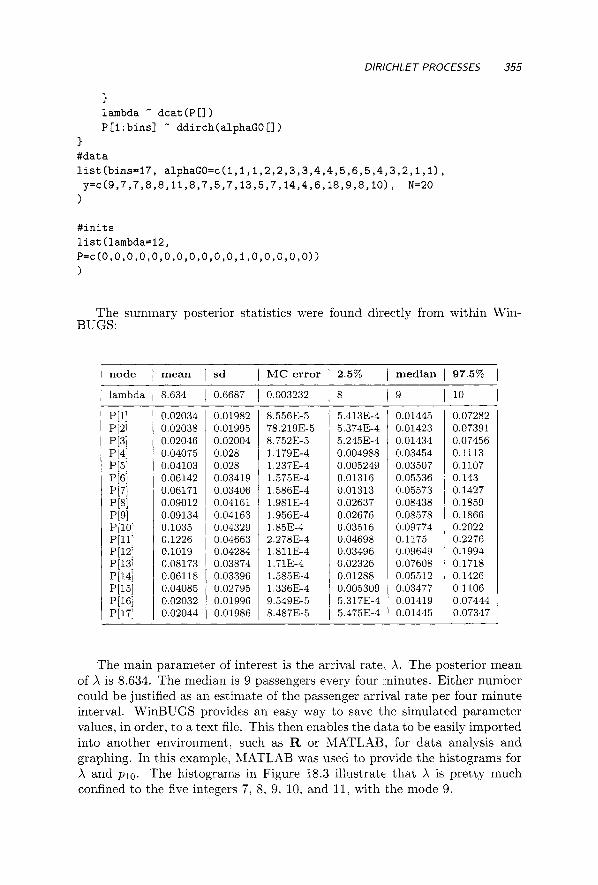
DIRICHLET PROC€SS€S 355
3 lambda dcat (P [I P [l :bins] ddirch(alphaG0 [I
> #data list (bins=17, alphaGO=c(l, 1,1,2,2,3,3,4,4,5,6,5,4,3,2,1,1) , y=c(9,7,7,8,8,11,8,7,5,7,13,5,7,14,4,6,18,9,8,10), N=20
)
#inits list(lambda=l2, P=c(0,0,0,0,0,0,0,0,0,0,0,1,0,0,0,0,0~) )
The summary posterior statistics were found directly from within Win- BUGS:
1 node 1 mean 1 sd 1 MC error I 2.5% 1 median 1 97.5% I 1 lambda 1 8.634 I 0.6687 I 0.003232 I 8 I9 I 10 I
0.02034 0.02038 0.02046 0.04075 0.04103 0.06142 0.06171 0.09012 0.09134 0.1035 0.1226 0.1019 0.08173 0.061 18 0.04085 0.02032 0.02044
0.01982 0.01995 0.02004 0.028 0.028 0.03419 0.03406 0.04161 0.04 163 0.04329 0.04663 0.04284 0.03874 0.03396 0.02795 0.01996 0.01986
8.5563-5 78.2 19E-5 8.7523-5 1.1793-4 1.237E-4 1.5753-4 1.5863-4 1.9813-4 1.9563-4 1.853-4
1.811E-4 1.71E-4 1.5853-4 1.3363-4 9.5493-5
2.2783-4
8.4873-5
5.4133-4 5.3743-4 5.2453-4 0.004988 0.005249 0.01316 0.01313 0.02637 0.02676 0.03516 0.04698 0.03496 0.02326 0.01288 0.005309 5.3173-4 5.4753-4
0.01445 0.01423 0.01434 0.03454 0.03507 0.05536 0.05573 0.08438 0.08578 0.09774 0.1175 0.09649 0.07608 0.05512 0.03477 0.01419 0.01445
0.07282 0.07391 0.07456 0.1113 0.1107 0.143 0.1427 0.1859 0.1866 0.2022 0.2276 0.1994 0.1718 0.1426 0.1106 0.07444 0.07347
The main parameter of interest is the arrival rate, A. The posterior mean of X is 8.634. The median is 9 passengers every four iminutes. Either number could be justified as an estimate of the passenger arrival rate per four minute interval. WinBUGS provides an easy way to save the simulated parameter values, in order, to a text file. This then enables the data to be easily imported into another environment. such as R or MATLAB, for data analysis and graphing. In this example, MATLAB was used to provide the histograms for X and p lo . The histograms in Figure 18.3 illustrate that X is pretty much confined to the five integers 7. 8. 9. 10. and 11, with the mode 9.

356 NONPARAMETRIC BAYES
Fig. 18.3 Histograms of 40,000 samples from the posterior for X and P[10].
18.1.2 Generalizing Dirichlet Processes
Some popular NP Bayesian models employ a mixture of Dirichlet processes. The motivation for such models is their extraordinary modeling flexibility. Let X I , Xa, . . . , X , be the observations modeled as
XiIOi - Bin(nz,Oz), OilF - F, i = l , . . . , n
F - Dir(a) .
(18.3)
If Q assigns mass to every open interval on [0,1] then the support of the distributions on F is the class of all distributions on [0,1]. This model allows for pooling information across the samples. For example, observation X, will have an effect on the posterior distribution of 0 3 . j # i, via the hierarchical stage of the model involving the common Dirichlet process.
The model (18.3) is used extensively in the applications of Bayesian non- parametrics. For example, Berry and Christensen (1979) use the model for the quality of welding material submitted to a naval shipyard, implying an interest in posterior distributions of 0,. Liu (1996) uses the model for re- sults of flicks of thumbtacks and focusses on distribution of O,+llX1,. . . , X,. McEarchern. Clyde, and Liu (1999) discuss estimation of the posterior pre- dictive Xn+l /X1. . . . . X,, and some other posterior functionals.
The DP is the most popular nonparametric Bayes model in the literature (for a recent review, see MacEachern and Mueller, 2000). However, limiting the prior to discrete distributions may not be appropriate for some applica-

BAYESIAN CATEGORICAL MODELS 357
tions. A simple extension to remove the constraint of discrete measures is to use a convoluted DP:
This model is called Dzrrchlet Process Mzxture (DPM). because the mix- ing is done by the DP. Posterior inference for DMP models is based on MCMC posterior simulation. Most approaches proceed by introducing la- tent variables d % X,ld, - f(xid,).O,(G - G and G‘ w DP(aG0). Efficient MCMC simulation for general MDP models is discussed, among others. in Escobar (1994), Escobar and West (1995), Bush and MacEachern (1996) and MacEachern and Mueller (1998). Using a Gaussian kernel, f ( z lp , C) 0:
exp{(z - p)’)E(z - p ) / 2 } . and mixing with respect to d = (p . C ) , a density estimate resembling traditional kernel density estimation is obtained. Such approaches have been studied in Lo (1984) and Escobar and West (1995).
A related generalization of Dirichlet Processes is i;he Mzxture of Dzrzchlet Processes (MDP). The MDP is defined as a DP with a center CDF which depends on random 0.
F - DP(aGe)
0 N 7 r ( d ) .
Antoniak (1974) explored theoretical properties of MDP’s and obtained pos- terior distribution for 0.
18.2 BAYESIAN CONTINGENCY TABLES AND CATEGORICAL MODELS
In contingency tables, the cell counts N,, can be modeled as realizations from a count distribution, such as Multinomial Mn(n,p,,) or Poisson P(A,,). The hypothesis of interest is independence of row and column factors. H0 : p,, = a,b,, where a, and b, are marginal probabilities of levels of two factors satisfying Etaz = C,b, = 1.
The expected cell count for the multinomial distribution is ENzJ = npt3. Under Ho, this equals na,b,, so by taking the logarilhm on both sides, one obtains

358 NONPARAMETRIC BAYES
Morning Noon
Afternoon Evening
for some parameters a, and @,. This shows that testing the model for addi- tivity in parameters a and p is equivalent to testing the original independence hypothesis Ho. For the Poisson counts, the situation is analogous: one uses log A,, = const + a, + D,.
Example 18.4 Activities of Dolphin Groups Revisited. We revisit the Dolphin’s Activity example from p. 162. Groups of dolphins were observed off the coast of Iceland and the table providing group counts is given below. The counts are listed according to the time of the day and the main activity of the dolphin group. The hypothesis of interest is independence of the type of activity from the time of the day.
6 28 38 6 4 5 14 0 9 13 56 10
1 Travelling Feeding Socializing
The WinBUGS program implementing the additive model is quite simple. We assume the cell counts are assumed distributed Poisson and the logarithm of intensity (expectation) is represented in an additive manner. The model parts (intercept, a,, and p J ) are assigned normal priors with mean zero and precision parameter xi. The precision parameter is given a gamma prior with mean 1 and variance 10. In addition to the model parameters, the WinBUGS program will calculate the deviance and chi-square statistics that measure goodness of fit for this model.
model { for (i in 1:nrow) {
for (j in 1:ncol) C groups[i, jl - dpois(lambda[i, jl) log(lambda[i,j]) <- c + alpha[il + beta[jl 1 )
#
c - dnorm(0, xi) for (i in 1:nrow) { alpha[i] dnorm(0, xi) 1 for (j in 1:ncol) { beta[jl I dnorrn(0, xi) 1 xi - dgauuna(0.01, 0.01)
# for (i in 1:nrow) C
for (j in 1:ncol) { devG[i, j] <- groups[i, j] * log((groups[i,jl+O.5)/ (lambda [i , j 1 +O .5) ) - (groups [i , j 1 -lambda [i , j 1 ; devX[i,jl <- (groups[i,jl-lambda[i,jl)
*(groups [it jl -lambda[i, jl ) /lambda[i, jl ; 1 > G2 <- 2 * sum( devG[,] 1 ; X2 <- sum( devX[,] ))

B A Y W A N CAT€GOR/CAL MOD€LS 359
1.514 1.028 -0.5182 -0.1105 1.121 0.1314 0.9439 0.5924 1.514 77.8 77.73
The data are imported as
0.7393 0.5658 0.5894 0.5793 0.5656 0.6478 0.6427 0.6451 0.7393 3.452 9.871
list(nrow=4, ncol=3, groups = s t ruc tu re (
.Data = c ( 6 , 28, 38, 6, 4, 5, 14, 0, 9, 13, 56, 101, .Dim,=c(4,3)) )
and initial parameters are
l i s t ( x i = O . l , c = 0 , a lpha=c(0 ,0 ,0 ,0) , beta=c(0,0,0) )
The following output gives Bayes estimators of tbe parameters, and mea- sures of fit. This additive model conforms poorly to the observations; under the hypothesis of independence, the test statistic is x 2 with 3 x 4 - 6 =
6 degrees of freedom, and the observed value X 2 = 77.73 has a pvalue (I-chi2cdf (77.73, 6 ) ) that is essentially zero.
I node
C
alpha[l] alpha[2] alpha[3] alpha[4] beta[l] beta[2] bet a[3]
G2 x2
C
mean I sd MC error I 2.5%
0.03152 0.0215 0.02072 0.02108 0.02 158 0.02492 0.02516 0.02512 0.03152 0.01548 0.03737
-0.02262 - 0.07829 -1.695 -1.259 0.02059 -1.134 -0.3026 -0.6616 - 0.02262 73.07 64.32
median
1.536 1.025 -0.5166 -0.1113 1.117 0.1101 0.9201 0.5687 1.536 77.16 75.85
97.5%
2.961 2.185 0.6532 1.068 2.277 1.507 2.308 1.951 2.961 86.2 102.2
Example 18.5 CEsarean Section Infections Rlevisited. We now con- sider the Bayesian solution to the Czesarean section birth problem from p. 236. The model for probability of infection in a birth by Cmarean section was given in terms of the logat link as,
P ( i n f ec t ion) = ,& + noplan + f l 2 r i s k f a c + p3 a n t i b i o .
log P ( n o i n f e c t i o n )
The WinBUGS program provided below implements the model in which the number of infections is Bin(n. p ) with p connected to covariates noplan r i s k f a c and a n t i b i o via the logit link. Priors on coefficients in the linear predictor are set to be a vague Gaussian (small precision parameter).
model( f o r ( i i n l:N)(
inf [i] - dbin(pCi1 , t o t a l [ i ] ) l o g i t ( p [ i ] ) <- beta0 + betal*noplan[i] +

360 NONPARAMETRIC BAYES
beta0 b e t a l be ta2 b e t a 3
be ta2*r i skf a c [i] + beta3*ant ib io [i]
3 be ta0 -dnorm(O, ~ . o ~ ~ ~ ~ ) b e t a l -dnorm(O, 0 . 0 0 0 0 ~ ) b e t a 2 "dnorm(0, 0.00001) b e t a 3 "dnorm(0, 0 . 0 0 0 0 ~ )
>
-1.962 0.4283 0.004451 -2.861 -1.941 -1.183 1.115 0.4323 0.003004 0.29 1.106 1.988 2.101 0.4691 0.004843 1.225 2.084 3.066 -3.339 0.4896 0.003262 -4.338 -3.324 -2.418
#DATA l i s t ( i n f = c ( l , 11, 0 , 0 , 28, 23, 8, 01,
noplan = c ( 0 , 1 , 0 , 1 , 0 9 1 , 0 , 1 ) , r i s k f a c = c ( l , l , 0 , 0, 1,1, 0, 01, a n t i b i o = c ( l , l , l,l,O,O,O,O) , N=8)
t o t a l = c(18 , 98, 2 , 0 , 58, 26, 40, 91,
#INITS l ist (be ta0 =0, betal=O,
beta2=0, beta3=0)
The Bayes estimates of the parameters Po - p3 are given in the WinBUGS output below.
I node 1 mean 1 sd 1 MC error 1 2.5% I median 1 97.5% 1
Note that Bayes estimators are close to the estimators obtained in the frequen- tist solution in Chapter 12: (po,&.p2,@3) = (-1.89, 1.07, 2.03. -3.25) and that in addition to the posterior means, posterior medians and 95% credible sets for the parameters are provided. WinBUGS can provide various posterior location and precision measures. From the table. the 95% credible set for PO is [-2.861. -1.1831.
18.3 BAYESIAN INFERENCE IN INFINITELY DIMENSIONAL NONPARAMETRIC PROBLEMS
Earlier in the book we argued that many statistical procedures classified as nonparametric are, in fact, infinitely parametric. Examples include wavelet regression, orthogonal series density estimators and nonparametric MLEs (Chapter 10). In order to estimate such functions, we rely on shrinkage, tapering or truncation of coefficient estimators in a potentially infinite ex- pansion class. (Chencov's orthogonal series density estimators, Fourier and wavelet shrinkage, and related.) The benefits of shrinkage estimation in statis-

INFINITELY DIMENSIONAL PROBLEMS 361
tics were first explored in the mid-1950's by C. Stein In the 1970's and 1980's. many statisticians were active in research on statistical properties of classical and Bayesian shrinkage estimators.
Bayesian methods have become popular in shrinkage estimation because Bayes rules are. in general, 9hrinkers". Most Bayes rules shrink large coef- ficients slightly, whereas small ones are more heaviily shrunk. Furthermore, interest for Bayesian methods is boosted by the possibility of incorporating prior information about the function to model wavelet coefficients in a realistic way.
Wavelet transformations W are applied to noisy measurements yz = f , + E , , i = 1.. . . , n, or, in vector notation, y = f + E . The linearity of W implies that the transformed vector d = W(y) is the sum of the transformed signal 8 = W ( f ) and the transformed noise 7 = W ( E ) . Furthermore, the orthog- onality of W implies that E ~ , i.i.d. normal N(0,o') components of the noise vector E . are transformed into components of 7 with the same distribution.
Bayesian methods are applied in the wavelet djomain, that is, after the wavelet transformation has been applied and the model d , N N(6',, a'). z = 1,. . . , n, has been obtained. We can model coefficient-by-coefficient because wavelets decorrelate and d, 's are approximately independent.
Therefore we concentrate just on a single typical wavelet coefficient and one model: d = 6' + E . Bayesian methods are applied to estimate the loca- tion parameter 6'. As 6''s correspond to the function to be estimated, back- transforming an estimated vector 8 will give the estimator of the function.
18.3.1 BAMS Wavelet Shrinkage
BASIS (stands for Bayeszan Adaptzve Multascale Shrznkage) is a simple effi- cient shrinkage in which the shrinkage rule is a Bayes rule for properly selected prior and hyperparameters of the prior. Starting with [die. 0'1 N N(6'. 0') and the prior 0' N € ( p ) , p > 0, with density f(a'1p) == pe-pu2, we obtain the marginal likelihood
1 2
dl6' N D€ (6' . . with density f(di6') = - fie-fild-el
If the prior on 6' is a mixture of a point mass 60 at zero, and a double- exponential distribution.
6 ' l E N €60 + (1 - €)D€(O, T ) ,
then the posterior mean of 6' (from Bayes rule) is:
(18.4)
(18.5)

362 NONPARAMETRlC BAYES
where
(18.6)
and
Fig. 18.4 Bayes rule (18.7) and comparable hard and soft thresholding rules.
As evident from Figure 18.4, the Bayes rule (18.5) falls between comparable hard- and soft-thresholding rules. To apply the shrinkage in (18.5) on a specific problem, the hyperparameters p, 7 , and E have to be specified. A default choice for the parameters is suggested in Vidakovic and Ruggeri (2001); see also Antoniadis, Bigot, and Sapatinas (2001) for a comparative study of many shrinkage rules, including BAMS. Their analysis is accompanied by MATLAB routines and can be found at
http://www-lmc.imag.fr/SMS/software/Gaussi~WaveDen/.
Figure 18.5(a) shows a noisy doppler function of size n = 1024, where the signal-to-noise ratio (defined as a ratio of variances of signal and noise) is 7. Panel (b) in the same figure shows the smoothed function by BAMS. The graphs are based on default values for the hyperparameters.
Example 18.6 Bayesian Wavelet Shrinkage in WinBUGS. Because of the decorrelating property of wavelet transforms, the wavelet coefficients are modeled independently. A selected coefficient d is assumed to be normal

/N f /N/T€LY DlMEiVSlONAL PROBLEMS 363
fig. 18.5 Signal reconstructed by BAMS.
(a) A noisy doppler signal [SKR=7, n=1024, noise variance cz = 11. (b)
d N N ( Q , 6 ) where Q is the coefficient corresponding to the underlying signal in data and < is the precision, reciprocal of variance. The signal component 6' is modeled as a mixture of two double-exponential distributions with zero mean and different precisions. because WinBUGS will not allow a point mass prior. The precision of one part of the mixture is large (so the variance is small) indicating coefficients that could be ignored as negligible. The cor- responding precision of the second part is small (so the variance is large) indicating important coefficients of possibly large magnitude. The densities in the prior mixture are taken in proportion p : (1 - p ) where p is Bernoulli. For all other parameters and hyperparameters. appropriate prior distributions are adopted.
We are interested in the posterior means for 8. Here is the WinBUGS implementation of the described model acting on ;some imaginary wavelet coefficients ranging from -50 to 50, as an illustration. Figure 18.6 shows the Bayes rule. Note a desirable shape close to that of the thresholding rules.
modelf f o r (j in 1:N)C
DD[j] dnorm(thetaCj1, tau) ; theta[j] <- pCjl * mulCj1 + (1-pCjl) * mu2Cjl; mul[jl ddexp(0, taul); muZ[jl ,, ddexp(0, tad); p[j] dbern(r) ;
3 r - dbeta(1,lO) ; tau - dgamma(0.5, 0.5) ;

364 NONPARAMETRIC BAYES
tau1 - dgamma(0.005, 0.5); tau2 -dgamma(0.5, 0.005);
#data list( DD=c(-50, -10, -5,-4,-3,-2,-1,-0.5, -0.1, 0,
0.1, 0.5, 1, 2,3,4,5, 10, 501, N = 1 9 ) ;
#inits list (tau=i, taul=O.i, tau2=i0) ;
Fig. 18.6 Approximation of Bayes shrinkage rule calculated by WinBUGS.
18.4 EXERCISES
18.1. Show that in the DP Definition 18.2, IE(C:==lwi) = 1 - [a/(l - a)]’.
18.2. Let p = s-”, ydG(y) and let G be a random CDF with Dirichlet process prior DP(aG0). Let y be a sample of size n from G. Using (18.2): show that
In other words, show that the expected posterior mean is a weighted average of the expected prior mean and the sample mean.
18.3. Redo Exercise 9.13, where the results for 148 survey responses are broken

EXERCISES 365
down by program choice and by race. Test the fit of the properly set additive Bayesian model. Use WinBUGS for model analysis.
18.4. Show that m(d) and S(d) from (18.6) and (18.7) are marginal distribu- tions and the Bayes rule for the model is
die DE ( e , 6) , e D E ( O . ~ ) ,
where p and r are the hyperparameters
18.5. This is an open-ended question. Select a data set with noise present in it (a noisy signal). transform the data to the wavelet domain, apply shrinkage on wavelet coefficients by the Bayes procedure described be- low, and back-transform the shrunk coefficients to the domain of original data.
(i) Prove that for [die] - N(O.1). [Olr2] N N(0,r2) , and r2 N (r2)-3/4% the posterior is unimodal at 0 if 0 < d2 < 2 and bimodal otherwise with the second mode
2
(ii) Generalize to [die] - N(O, u 2 ) . u2 known, and apply the larger mode shrinkage. Is this shrinkage of the thresholding type?
(iii) Use the approximation (1 - u)" N (1 - cyu) for u small to argue that the largest mode shrinkage is close to a James-Stein-type rule S*(d) =
(1 - &)+ d, where (f)+ = max(0, f}.
18.6. Chipman, Kolaczyk, and McCulloch (1997) prolpose the following model for Bayesian wavelet shrinkage (ABWS) which we give in a simplified form,
The prior on 6' is defined as a mixture of two normals with a hyperprior on the mixing proportion,
Variance o2 is considered known. and c >> 1
i) Show that the Bayes rule (posterior expectation) for 0 has the explicit form of

366 NONPARAMETRIC BAYES
where
d d l y = 1) p r ( d l y = 1) + (1 - p)7r(dly = 0)
P ( y = lid) =
and 7r(dlr = 1) and 7r(d(y = 0) are densities of N(0,a2 + ( c T ) ~ ) and N(0, a’ + T’ ) distributions, respectively, evaluated at d.
(ii) Plot the Bayes rule from (i) for selected values of parameters and hyperparameters (0’; T * , y, c ) so that the shape of the rule is reminiscent of thresholding.
REFERENCES
Antoniadis, A., Bigot, J., and Sapatinas, T. (2001); “Wavelet Estimators in Nonparametric Regression: A Comparative Simulation Study,” Journal of Statistical Software, 6, 1-83.
Antoniak, C. E. (1974), “Mixtures of Dirichlet Processes with Applications to Bayesian Nonparametric Problems,” Annals of Statistics, 2, 1152-1174.
Berry, D. A., and Christensen, R. (1979), “ Empirical Bayes Estimation of a Binomial Parameter Via Mixtures of Dirichlet Processes,” Annals of Statistics, 7, 558-568.
Bush, C. A., and MacEachern S. N. (1996)) “A Semi-parametric Bayesian Model for Randomized Block Designs,” Biometrika, 83, 275-286.
Chipman, H. A., Kolaczyk, E. D., and McCulloch, R. E. (1997), “Adaptive Bayesian Wavelet Shrinkage,” Journal of American Statistical Associa- tion, 92, 1413-1421.
Escobar, M. D. (1994), “Estimating Normal Means with a Dirichlet Process Prior,” Journal of American Statistical Association, 89, 268-277.
Escobar, M. D., and West, M. (1995), “Bayesian Density Estimation and Inference Using Mixtures, Journal of American Statistical Association,
Fabius, J . (1964), “Asymptotic Behavior of Bayes’ Estimates,” Annals of Mathematical Statistics, 35, 846-856.
Ferguson, T. S. (1973): “A Bayesian Analysis of Some Nonparametric Prob- lems,” Annals of Statistics, 1, 209-230.
(1974) , “Prior Distributions on Spaces of Probability Measures,” Annals of Statistics, 2, 615-629.
Freedman, D. A. (1963), “On the Asymptotic Behavior of Bayes’ Estimates in the Discrete Case,” Annals of Mathematical Statistics, 34, 1386-1403.
Liu, J. S. (1996), “ Nonparametric Hierarchical Bayes via Sequential Imputa-
90, 577-588.

REFERENCES 367
tions,” Annals of Statistics, 24, 911-930. Lo, A. Y. (1984), “On a Class of Bayesian Nonpararnetric Estimates, I. Den-
sity Estimates,“ Annals of Statistics, 12, 351-357. MacEachern, S. N., and Mueller, P. (1998), “Estimating Mixture of Dirichlet
Process Models, Journal of Computational and Graphical Statistics, 7,
(2000), “Efficient MCMC Schemes for Robust Model Extensions Us- ing Encompassing Dirichlet Process Mixture Models,” in Robust Bayesian Analysis, Eds. F. Ruggeri and D. Rios-Insua, New York: Springer Ver- lag.
MacEachern, S. N., Clyde, M . , and Liu, J. S. (19’99), “Sequential Impor- tance Sampling for Xonparametric Bayes Models: The Next Genera- tion,“ Canadian Journal of Statistics, 27, 251-267.
Mueller, P., and Quintana, F. A. (2004), “Nonparametric Bayesian Data Anal- ysis,” Statistical Science, 19. 95-110.
Sethuraman, J., and Tiwari, R. C. (1982), “Convergence of Dirichlet Measures and the Interpretation of their Parameter,” in Statistical Decision Theory and Related Topics 111, eds. S . Gupta and J. 0. Berger; New York: Springer Verlag, 2, pp. 305-315.
Sethuraman, J. (1994), “A Constructive Definition o’f Dirichlet Priors,‘’ Sta- tistica Sinica, 4, 639-650.
Vidakovic, B., and Ruggeri, F. (2001), ”BAMS Method: Theory and Simula- tions.” Sankhya, Ser. B, 63, 234-249.
223-238.

This Page Intentionally Left Blank

Appendix A: MATLAB
The combination of some data and an aching desire for an answer does not ensure that a reasonable answer can be extracted from a given body of data.
J. W. Tukey (1915-2000)
A . l USING MATLAB
MATLAB is a interactive environment that allows t'he user to perform compu- tational tasks and create graphical output. The user types in expressions and commands in a Command Window where numerical results of the commands are displayed with the user input. Graphical output will be produced in a new (graphics) window that can usually be printed1 or stored.
When MATLAB is launched. several windows are available to the user as you can see in Fig. A.7. Their uses are listed below:
Command Window: Typing commands and expressions - this is the main interactive window in the user interface
Launch Pad Window: Allows user to run demos
Workspace Window: List of variables entered or created during ses- sion
369

370 Appendix A: MATLAB
Fig. A. 7 Interactive environment of LIATLAB.
0 Command History Window: List of recent commands used
0 Array Editor Window: Allows user to manipulate arrays variables using spreadsheet
0 Current Directory Window: To specify directory where MATLAB will search for or store files
MATLAB is a high-level technical computing language for algorithm de- velopment, data visualization, data analysis, and numeric computation. Some highlight features of MATLAB can be summarized as
0 High-level language for technical computing. which are easy to learn
0 Development environment for managing code, files. and data
0 Mathematical functions for linear algebra. statistics, Fourier analysis. filtering. optimization, and numerical integration
0 2-D and 3-D graphics functions for visualizing data
0 Tools for building custom graphical user interfaces
0 Functions to communicate with other statistical software. such as R. WinBUGS

USlNG MATLAB 371
To get started, you can type doc in the command window. This will bring you to an HTML help window and you can search keyword or browse topics therein.
>> doc
Fig. A.8 Help window of MATLAB.
If you know the function name, but do not know how to use it, it is often useful to type "help function name" in command window. For example, if you want to know how to use function randg or find out what randg does.
>> h e l p randg
RANDG Gamma random numbers ( u n i t s c a l e ) . Note: To genera te gamma random numbers with s p e c i f i e d shape and s c a l e parameters , you should c a l l GAMRND.
R = RANDG r e t u r n s a s c a l a r random value chosen from a gamma d i s t r i b u t i o n with u n i t s c a l e and shape.
R = RANDG(A) r e t u r n s a mat r ix of random values chosen from gamma d i s t r i b u t i o n s with u n i t s c a l e . R i s t h e same s i z e as A, and RANDG genera tes each element of R us ing a shape parameter equal t o t h e corresponding element of A . . . . .

372 Appendix A: MATLAB
A . l . l Toolboxes
Serving as extensions to the basic MATLAB programming environment, tool- boxes are available for specific research interests. Toolboxes available include
Communications Toolbox Control System Toolbox DSP Blockset Extended Symbolic Math Toolbox Financial Toolbox Frequency Domain System Identification Fuzzy Logic Toolbox Higher-Order Spectral Analysis Toolbox Image Processing Toolbox LMI Control Toolbox Mapping Toolbox Model Predictive Control Toolbox Mu-Analysis and Synthesis Toolbox NAG Foundation Blockset Neural Network Toolbox Optimization Toolbox Partial Differential Equation Toolbox QFT Control Design Toolbox Robust Control Toolbox Signal Processing Toolbox Spline Toolbox Statistics Toolbox System Identification Toolbox Wavelet Toolbox
For the most part we use functions in the base MATLAB product, but where necessary we also use functions from the Statistics Toolbox. There are numer- ous procedures from other toolboxes that can be helpful in nonparametric data analysis (e.g., Neural Network Toolbox, Wavelet Toolbox) but we restrict rou- tine applications to basic and fundamental computational algorithms to avoid making the book depend on any pre-written software code.
A.2 M A T R I X OPERATIONS
MATLAB was originally written to provide easy interaction with matrix soft- ware developed by the NASA1-sponsored LINPACK and EISPACK projects. Today, MATLAB engines incorporate the LAPACK and BLAS libraries, em- bedding the state of the art in software for matrix computation. Instead of
'National Aeronautics and Space Administration.

MATRIX OPERATIONS 373
relying on do loops to perform repeated tasks, IIA'TLAB is better suited to using arrays because MATLAB is an interpreted language.
MATLAB was originally written to provide easy access to matrix software developed by the LINPACK and EISPACK projects, ( these projects were sponsored by NASA and much of the source code is in public domain) which together represent the state-of-the-art in software for matrix computation.
A.2.1 Entering a Matrix
There are a few basic conventions of entering a ma,trix in MATLAB, which include
0 Separating the elements of a row with blanks or commas.
0 Using a semicolon ':' to indicate the end of each row.
0 Surrounding the entire list of elements with square brackets, [
>> A = C3 0 1; 1 2 1; 1 1 11 % columns separa ted by a space % rows separa ted by " ; "
A = 3 0 1 1 2 1 1 1 1
A.2.2 Arithmetic Operations
MATLAB uses familiar arithmetic operators and precedence rules, but unlike most programming languages, these expressions involve entire matrices. The common matrix operators used in MATLAB are listed as follows:
+ addition - subtraction * multiplication power ' transpose .' transpose \ left division / right divisiion .* element-wise multiplication . A element-wise power ./ element-wise right division
>> X=[lO 10 201 ' ; >> A*X % A is 3x3, X is 3x1 and X' is lx
% semicolon suppresses output of X
% so A*X is 3x1 ans =
50 50 40

374 Appendix A: MATLAB
>> y=A\X % y is the solution of Ay=X
Y = -10.0000 -10.0000 40.0000
>> A.*A % " . * " multiplies corresponding elements of % matching matrices; this is equivalent to A.-2
ans =
9 0 1 1 4 1 I 1 1
A.2.3 Logical Operations
The relational operators in MATLAB are
< less than > greater than <= less-than-or-equal __ >= greater-than-or-equal -= not equal & (logical) and 1 (logical) or N (logical) not
equal __
When relational operators are applied to scalars, 0 represents false and 1 represents true.
A.2.4 Matrix Functions
These extra matrix functions are helpful in creating and manipulating arrays:
eye identity matrix ones matrix of ones zeros matrix of zeros diag diagonal matrix rand matrix of random U(0,l) inv matrix inverse det matrix determinant rank rank of matrix find indices of nonzero entries norm normalized matrix
A.3 CREATING FUNCTIONS IN MATLAB
Along with the extensive collection of existing MATLAB functions, you can create your own problem-specific function using input variables and generating

IMPORTING AND EXPORTING DATA 375
array or graphical output. Once you look at a simple example, you can easily see how a function is constructed. For example, here is a way to compute the PDF of a triangular distribution, centered at zero with the support [-c. c]:
function y = tripdf(x,c) y l = max(O,c-abs(x)) / c-2; Y = Yl
The function starts with the function y = functionname(input) where y is just a dummy variable assigned as function output at the end of the function. Local variables (such as y l ) can be defined and combined with input variables (x,c) and the output can be scalar or matrix form. Once the function is named. it will override any previous function with the same name (so try not to call your function "sort", "inv" or any other known MATLAB function you might want to use later).
The function can be typed and saved as an m-file (i.e., tripdf .m) because that is how MATLAB recognizes an external file with executable code. Al- ternatively, you can type the entire function (line b;y line) directly into the program, but it won't be automatically saved after you finish. Then you can '.call" the new function as
>> v = tripdf(0:4,3)
v = co.3333 0.2222 0.1111 0 03
>> tripdf ( -1 ,Z) <= 0.5 % =1 if statement is true ans =
1
It also possible to define a function as a variable. For example, if you want to define a truncated (and unnormalized) normal PDF, use the following command
>> tnormpdf = a(x, mu, sig, left, right) . . .
>> tnormpdf (-3:3,0,1,-2,2) normpdf (x,mu,sig) .*(x>left & x <right);
ans =
0 0 0.2420 0.3989 0.2420 0 0
The tnormpdf function does not integrate to 1. To normalize it, one can di- vide the result by (normcdf (right ,mu,sigma) - normcdf (left ,mu,sigma)) .
A.4 IMPORTING AND EXPORTING DATA
As a first step of data analysis, we may need to import data from external sources. The most common types of files used in the MATLAB statistical

376 Appendix A: MATLAB
computing are MATLAB data files, Text files, and Spreadsheet files. The MATLAB data file has the extension name * .mat. Here is an example of importing such data to MATLAB workspace.
A.4.1 M A T Files
You can use the command whos to look what variables are in the data file.
>> whos -file dataexample
Name Size Bytes Class
Sigma 2x2 U S 1x1 mu 1x2 xx 500x2
32 double array 8 double array 16 double array
8000 double array
Grand total is 1007 elements using 8056 bytes
Then you can use the command load to load all variables in this data file.
>> clear >> load dataexample >> whos
% clear variables in the workspace
% check what variables a r e in the workspace
Name Size Bytes Class
Sigma 2x2 anS 1x1 mu 1x2 xx 500x2
32 double array 8 double array 16 double array
8000 double array
Grand total is 1007 elements using 8056 bytes
In some cases, you may only want to load some variables in the MAT file to the workspace. Here is how you can do it.
>> clear >> varlist = {’Sigma’,’mu’); >> load(’dataexample.mat’,varlistC:)) >> clear varlist >> whos
% Created a list of variables
% remove varlist from workspace % see what is in the workspace
Name Size Bytes Class

IMPORTlNG AND EXPORTING DATA 377
Sigma 2x2 mu 1x2
32 double array 16 double array
Grand total is 6 elements using 48 bytes
Another way of creating variables of interest is to use an index.
>> clear >> vars = whos(’-file’, ’dataexample.mat’); >> load( ’ dataexample .mat ’ ,vars ( [l ,3] ) .name)
If you do not want to use full variable names, but want to use some patterns in these names. the load command can be used with a ‘-regexp‘ option. The following command will load the same variable as the previous one.
>> load(’dataexample.mat’, ’-regexp’, ’-St-m’);
Text files usually have the ext,ension name * . t x t , * . d .a t , * . csv, and so forth.
A.4.2 Text Files
If the data in the text file are organized as a matrix, you can still use load to import the data into the workspace.
>> load mytextdata.dat >> mytextdata
mytextdata =
-0.3097 0.2950 -0.1681 -1.4250 -1.5219 -0.3927 -0.6873 0.4615 0.8265 0.5759 -0.9907 1.0915 -0.6130 -1.1414 -0.0498 -1.0443 0.9597 0.0611 0.7193 -2.8428 1.9730 0.0123 -0.2831 0.9968
You can also assign the loading data to be stored )in a new variable.
>> x = load(’mytextdata.dat’);
The command load will not work if the text file is not organized in matrix form. For example, if you have a text file mydata. t x t
>> type mydata. txt
var 1 var2 var3 var4 name -0.3097 0.2950 -0.1681 -1.4250 Olive -1.5219 -0.3927 -0.6873 0.4615 Richard

378 Appendix A: MATLAB
0.8265 0.5759 -0.9907 1.0915 Dwayne -0.6130 -1.1414 -0.0498 -1.0443 Edwin 0.9597 0.0611 0.7193 -2.8428 Sheryl 1.9730 0.0123 -0.2831 0.9968 Frank
You should use a new function txtread to import variables to workspace.
>> [vari ,var2 ,var3,var4, strl = . . . textread(’mydata.txt’,’%f%f%f%f%s’, ’headerlines’,l ) ;
Alternatively, you can use textscan to finish the import.
>> fid = fopen(’mydata.txt’); >> c = textscan(fid, ’%f%f%f%f%s’, ’headerLines’,l); >> f close (f id) ; >> [CC1:411 % varl - var4
ans = -0.3097 0.2950 -0.1681 -1.4250 -1.5219 -0.3927 -0,6873 0.4615 0.8265 0.5759 -0.9907 1.0915 -0.6130 -1.1414 -0.0498 -1.0443 0.9597 0.0611 0.7193 -2.8428 1.9730 0.0123 -0.2831 0.9968
ans = ’Olive’ ’Richard ’ ’Dwayne’ ’Edwin’ ’ Sheryl ’ Frank ’
Comma-separated values files are useful when exchanging data. Given the file data . csv that contains the comma-separated values
>> type data. csv
02, 04, 06, 08, 10, 12 03, 06, 09, 12, 15, 18 05, 10, 15, 20, 25, 30 07, 14, 21, 28, 35, 42 11, 22, 33, 44, 55, 66
You can use csvread to read the entire file into workspace
>> csvread(’data.csv’)

IMPORTING AN,D EXPORTING DATA 379
ans =
2 4 6 8 3 6 9 12 5 10 15 20 7 14 21 28 11 22 33 44
10 12 15 18 25 30 35 42 55 66
A.4.3 Spreadsheet Files
Data from a spreadsheet can be imported into the workspace using the func- tion xlsread.
>> [NUMERIC, TXT ,RAW] =xls read( ’ d a t a . x l s ’ 1 ; >> NUMERIC
NUMERIC =
1.0000 2.0000 3.0000 4.0000 5.0000 6.0000 7.0000 8.0000 9.0000
>> TXT
TXT = ’Date ’ ’1/1/2001’ ’1/2/2001’ ’1/3/2001’ ’1/4/2001’ ’1/5/2001’ ’1/6/2001’ ’1/7/2001’ ’1/8/2001’ ’1/9/2001’
>> RAW
RAW = ’Date ’ ’1/1/2001’ J1/2/2001’
0.3000 N a N 0.4500 N a N 0.3000 12.0000 0.3500 5.0000 0.3500 5.0000 0.3500 10.0000 0.3500 13.0000 0.3500 5.0000 0.3500 23.0000
’ v a r l ’ var2 ’ ’var3’
’ v a r l ’ c 11 c 21
’var2’ CO .30001 [O .45001
’name’ ’Frank’
’ Sheryl ’
’ 12i chard ’ ’ Olive ’ ’ Dwayne ’ ’ Edwin’ ’ ;:tan J
’ 9
, ’
’name’ ’Frank’ C N a N l
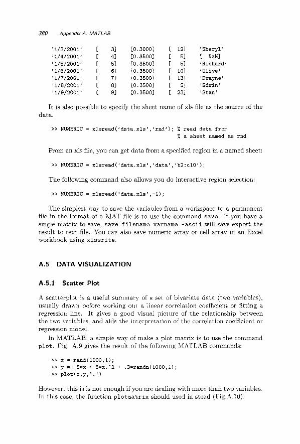
380 Appendix A: MATLAB
’1/3/2001’ [ 31 [0.3000] [ 121 ’Sheryl’ ’1/4/2001’ [ 41 [0.35001 I: 51 [: NaNl ’1/5/2001’ [ 51 [0.3500] [ 51 ’Richard’ ’1/6/2001’ [ 61 [0.3500] [ 101 ’Olive’ ’1/7/2001’ [ 71 [0.35001 131 ’Dwayne’ ’1/8/2001’ [ 81 [0.35001 [ 51 ’Edwin’ ’1/9/2001’ [ 91 C0.35001 [ 231 ’Stan’
It is also possible to specify the sheet name of xls file as the source of the data.
>> NUMERIC = xlsread(’data.xls’,’rnd’); % read data from % a sheet named as rnd
From an xls file, you can get data from a specified region in a named sheet:
>> NUMERIC = xlsread(’data.xls’,’data’,’b2:c10J);
The following command also allows you do interactive region selection:
>> NUMERIC = xlsread(’data.xls’,-l);
The simplest way to save the variables from a workspace to a permanent file in the format of a MAT file is to use the command save. If you have a single matrix to save, save filename varname - a s c i i will save export the result to text file. You can also save numeric array or cell array in an Excel workbook using x l s w r i t e .
A.5 DATA VISUALIZATION
A.5.1 Scatter Plot
A scatterplot is a useful summary of a set of bivariate data (two variables). usually drawn before working out a linear correlation coefficient or fitting a regression line. It gives a good visual picture of the relationship between the two variables, and aids the interpretation of the correlation coefficient or regression model.
In MATLAB, a simple way of make a plot matrix is to use the command p l o t . Fig. A.9 gives the result of the following MATLAB commands:
However. this is is not enough if you are dealing with more than two variables. In this case. the function p l o t m a t r i x should used in stead (Fig.A.lO).

DATA VISUALIZATION 381
-1 ’
0.2 0.4 0.6 0.8 1
Fig. A.9 Scatterplot of (z,y) for x = rand(1000,l) and y = .5*x + 5*x.2 + .3*randn(1000,1).
>> x = randn(50,3); >> y = x*[-l 2 1;2 0 1;l -2 3 ; l ’ ; >> plotmatrix(y)
In classification problems, it is also useful to look at scatter plot matrix with grouping variable (Fig.A. 11).
>> load carsmall; >> X = [MPG,Acceleration,Displacement,Weight,Horsepower] ; >> varNames = {’MPG’ ’Acceleration’ ’Displacement’ . . .
>> gplotmatrix(X, [I ,Cylinders, ’bgrcm’ , [ I , [I, ’on’, ’hist’ ,varNames) ; >> set(gcf,’color’,’white’)
’Weight’ ’Horsepower’);
A.5.2 Box Plot
Box plot is an excellent tool for conveying location and variation information in data sets. particularly for detecting and illustrating location and variation changes between different groups of data. Here is an example of how MATLAB makes a boxplot (Fig. A.12).
>> load carsmall >> boxplot(MPG, Origin, ’grouporder’, . . .
>> set(gcf,’color’,’white’) {’France’ ’Germany’ ’Italy’ ’Japan’ ’Sweden’ ’USA’))

382 Appendix A: MATLAB
Fig. A.10 Simulated data visualized by plotmatrix.
Fig. A . l l Scatterplot matrix for Car Data.

DATA VlSUALlZAJlON 383
45-
40
35
30
; 25- 20-
15-
10
+ '
-
T
I I I
I I
1- I I I El 0 Q - -
I
I
-
B I
I I
- I
Fig. A.12 Boxplot for Car Data.
A.5.3 Histogram and Density Plot
A histogram of univariate data can be plotted using hist (Fig.A.13).
>> hist (randn(100,l)
while a three-dimensional histogram of bivariate data is plotted using hist3, (Fig.A.14);
>> mu = [I -11; Sigma = L.9 .4 ; . 4 .31; >> r = mvnrnd(mu, Sigma, 500); >> hist3(r)
If you like a smoother density plot. you may turn to a kernel density or distribution estimate implemented in ksdensity (Fig.A.15). Also, in recent versions of MATLAB you have the option of not asking for outputs from the ksdensity, and the function plots the results directly.
>> [y,x] = ksdensity(randn(100,l)); >> plot (x ,y )
A.5.4 Plotting Function List
Here is a complete list of statistical plotting functions available in MATLAB

384 Appendix A: MATLAB
Fig. A.13 Histogram for simulated random normal data.
Fig. A. 14 Spatial histogram for simulated two-dimensional random normal data.

DATA V/SUAL/ZAT/ON 385
Fig. A.15 Kernel density estimator for simulated random normal data.
andrewsplot - Andrews plot for multivariate d,ata. bar - Bar graph. biplot - Biplot of variable/factor coefficients and scores. boxplot - Boxplots of a data matrix (one !per column). cdfplot - Plot of empirical cumulative distribution function. contour - Contour plot. ecdf - Empirical CDF (Kaplan-Meier estimate). ecdfhist - Histogram calculated from empirical CDF. fplot - Plots scalar function $f(x)$ at values of $x$. f surf ht - Interactive contour plot of a function. gline - Point, drag and click line drawing on figures. glyphplot - Plot stars or Chernoff faces fo:r multivariate data. gname - Interactive point labeling in x-y plots. gplotmatrix - Matrix of scatter plots grouped by a common variable. gscatter hist - Histogram (in MATLAB toolbox). hist3 ksdensity - Kernel smoothing density estimation. lsline - Add least-square fit line to scatter plot. normplot - Normal probability plot. parallelcoords - Parallel coordinates plot for multivariate data. probplot - Probability plot. q¶Plot - Quantile-Quantile plot. refcurve - Reference polynomial curve. ref line - Reference line. stairs - Stair-step of y with jumps at pt3ints x. surfht - Interactive contour plot of a data grid.
- Scatter plot of two variables g:rouped by a third.
- Three-dimensional histogram of bivariate data.

386 Appendix A: MATLAB
wblplot - Weibull probability plot.
A.6 STATISTICS
For your convenience! let’s look at a list of functions that can be used to compute summary statistics from data.
corr corrcoef
cross t ab geomean grpst at s harmmean iqr kurtosis mad mean median moment nancov nanmax nanmean nanmedian nanmin nanstd nansum nanvar
cov
- Linear or rank correlation coefficient. - Correlation coefficient with confidence intervals - Covariance. - Cross tabulation. - Geometric mean. - Summary statistics by group. - Harmonic mean. - Interquartile range. - Kurtosis. - Median Absolute Deviation. - Sample average (in MATLAB toolbox). - 50th percentile of a sample. - Moments of a sample. - Covariance matrix ignoring NaNs. - Maximum ignoring NaNs. - Mean ignoring NaNs. - Median ignoring NaNs. - Minimum ignoring NaNs. - Standard deviation ignoring NaNs. - Sum ignoring NaNs. - Variance ignoring NaNs.
partialcorr - Linear or rank partial correlation coefficient. prctile - Percentiles. quantile - Quantiles. range - Range. skewness - Skewness. std - Standard deviation (in MATLAB toolbox). tabulate - Frequency table. trimmean - Trimmed mean. var - Variance

STATlSTlCS 387
A.6.1 Distributions
I Distribution I CDF I PDF 1 Inveirse CDF I RNG 1
Beta Binomial Chi square Exponential Extreme value F Gamma Geometric Hypergeometric Lognormal Multivariate normal Negative binomial Normal (Gaussian) Poisson Rayleigh t Discrete uniform Uniform distribution Weibull
betacdf binocdf chi2cdf expcdf evcdf f cdf
gamcdf geocdf
hygecdf logncdf mvncdf
nbincdf normcdf
poisscdf r a y 1 cdf
t cdf unidcdf unif cdf wblcdf
betapdf binopdf chi2pdf exppdf evpdf fpdf
geopdf
lognpdf mvnpdf nbinpdf normpdf
p o i s spdf raylpdf
tpdf unidpdf unifpdf
wblpdf
gampdf
hygepdf
beitainv binoinv ch.i2inv expinv evinv :E i n v
gaminv ge o i n v
hygeinv lcgninv mvninv
nbininv ncrminv p o i s s i n v r a y l i n v
it i n v unidinv u n i f i n v wblinv
be tarnd binornd chi2rnd exprnd evrnd f rnd
gamrnd geornd
hygernd lognrnd mvnrnd
nbinrnd normrnd
poiss rnd r a y l r n d
t r n d unidrnd unif rnd wblrnd
A.6.2 Distribution Fitting
betaf it binof it evf it expf it gamf it gevf it gpf it lognf it m l e mlecov lognf it normf it poiss f it r a y l f it unif it wblf it
- Beta parameter es t imat ion . - Binomial parameter e s t i m a t i o n . - Extreme value parameter e s t i m a t i o n . - Exponent ia l parameter e s t i m a t i o n . - Gamma parameter es t imat ion . - General ized extreme va lue parameter es t imat ion . - General ized Pare to parameter es t imat ion . - Lognormal parameter e s t i m a t i o n . - Maximum l i k e l i h o o d es t imat ion (IrILE) . - Asymptotic covariance mat r ix of MLE. - Negative binomial parameter e s t i m a t i o n . - Normal parameter e s t i m a t i o n . - Poisson parameter es t imat ion . - Rayleigh parameter e s t i m a t i o n . - Uniform parameter e s t i m a t i o n . - Weibull parameter e s t i m a t i o n .
In addition to the command line function listed above, there is also a GUI to used for distribution fitting. You can use the command df ittool to invoke this tool (Fig.A.16).

388 Appendix A: MATLAB
>> dfittool
Fig. A.16 GUI for dfittool.
A.6.3 Nonparametric Procedures
kstest - Kolmogorov-Smirnov two-sample test. kst e st 2 mtest - Cramer Von Mises test for normality dagosptest runs-test - Runs test sign-test1 - Two-sample sign test. kruskal-wallis - Kruskal-Wallis rank test. friedman kendall spear - Spearman correlation coefficient. WmW - Wilcoxon-Mann-Whitney two-sample test. tablerxc mantel-haenszel- Mantel-Haenszel statistic for $2$x$2$ tables.
- Kolmogorov-Smirnov one or two-sample test
- D’Agostino-Pearson’s test for normality
- Friedman randomized block design test - Computes Kendall’s tau correlation statistic
- test of independence for $r$x$c$ table.
The listed nonparametric functions that are not distributed with MATLAB or its Statistics Toolbox can be downloaded from the book home page.

STATISTICS 389
A.6.4 Regression Models
A.6.4.1 Ordinary Least Squares (OLS) The most straightforward way of im- plementing OLS is based on normal equations.
>> x = rand(20,l); >> y = 2 + 3*x + randn(size(x)); >> X = [ones(length(x), 1) ,XI ; >> b = inv(X’*X)*X’*y % normal equation
b = 1.8778 3.4689
A better solution uses backslash because it is more numerically stable than inv.
b2 =
1.8778 3.4689
The pseudo inverse function pinv is also an option. It too is numerically stable, but it will yield subtly different results when your matrix is singular or nearly so. Is pinv better? There are arguments for both backslash and pinv. The difference really lies in what happens on singular or nearly singular matrixes. pinv will not work on sparse problems, and because pinv relies on the singular value decomposition, it may be slower for large problems.
>> b3 = pinvo()*y
b3 = 1.8778 3.4689
Large-scale problems where X is sparse may sometimes benefit from a sparse iterative solution. lsqr is an iterative solver
>> b4 = lsqr(X,y,l.e-13,10)
lsqr converged at iteration 2 to a solution wit.h relative residual 0.33

390 Appendix A: MATLAB
b4 =
I. 8778 3.4689
There is another option, Iscov. lscov is designed to handle problems where the data covariance matrix is known. It can also solve a weighted regression problem.
b5 = 1.8778 3.4689
Directly related to the backslash solution is one based on the QR factor- ization. If our over-determined system of equations to solve is X b = y , then a quick look at the normal equations,
b = (X’X)-lX’y
combined with the qr factorization of X ,
X = Q R
yields b = (R’Q’QR)-lR’Q‘y.
Of course, we know that Q is an orthogonal matrix, so Q’Q is an identity matrix.
b = (R’R)-‘R’Q’y
If R is non-singular, then (R’R)-‘ = R-’R‘-’? so we can further reduce to
b = R-lQ‘y
This solution is also useful for computing confidence intervals on the param- eters.
b6 = 1.8778 3.4689
A.6.4.2 Weighted Least Squares (WLS) Weighted Least Squares (WLS) is special case of Generalized Least Squares (GLS). It should be applied when

STATlSTlCS 391
there is heteroscedasticity in the regression. i.e. the variance of the error term is not a constant across observations. The optimal weights should be inversely proportional to the error variances.
>> x = (1:lO)’; >> wgts = l./rand(size(x)); >> y = 2 + 3*x + wgts.*randn(size(x)); >> X = [ones(length(x) ,1) ,XI ; >> b7 = lscov(M,y,wgts)
b7 =
-89.6867 27.9335
Another alternative way of doing WLS is to transform the independent and dependent variables so that we apply OLS to the transformed data.
coef8 = -89.6867 27.9335
A.6.4.3 Iterative Reweighted Least Squares (IRLS) IRLS can be used for mul- tiple purposes. One is to get robust estimates by r’educing the effect of out- liers. Another is to fit a generalized linear model, as described in Section A.6.6. MATLAB provides a function robus t f it which performs iterative reweighted least squares estimation which yield robust coefficient estimates.
brob =
10.5208 -2.0902
A.6.4.4 performs nonlinear least squares estimation.
Nonlinear Least Squares MATLAB provides a function nlinf it which
>> mymodel = @(beta, x) (beta(l)*x(: ,2) - x ( : ,3)/beta(5)) . / . . .
>> load reaction; (l+beta(2)*x(:,l)+beta(3)*~(:,2)+beta(4)*~(:,3));

392 Appendix A: MATLAB
>> beta = nlinfit(reactants,rate,mymodel,ones(5,1))
beta =
1.2526 0.0628 0.0400 0.1124 1.1914
A.6.4.5 Other Regression Functions
coxphfit nlintool nlpredci - Confidence intervals for prediction in nonlinear models nlparci - Confidence intervals for parameters in nonlinear models polyconf polyfit - Least-squares polynomial fitting. polyval rcoplot - Residuals case order plot. regress - Multivariate linear regression, also return the
- Cox proportional hazards regression. - Graphical tool for prediction in nonlinear models.
- Polynomial evaluation and with confidence intervals.
- Predicted values for polynomial functions.
R-square statistic, the F statistic and p value for the full model, and an estimate of the error variance.
regstats ridge - Ridge regression. rstool stepwise - Interactive tool for stepwise regression. stepwisefit - Non-interactive stepwise regression.
- Regression diagnostics for linear regression.
- Multidimensional response surface visualization (RSM).
A.6.5 ANOVA
The following function set can be used to perform ANOVA in a parametric or nonparametric fashion.
anoval - One-way analysis of variance. anova2 - Two-way analysis of variance. anovan - n-way analysis of variance. aoctool - Interactive tool for analysis of covariance. friedman - Friedman’s test (nonparametric two-way anova). kruskalwallis - Kruskal-Wallis test (nonparametric one-way anova)
A.6.6 Generalized Linear Models
MATLAB provides the glmf it and glmval functions to fit generalized linear models. These models include Poisson regression, gamma regression, and binary probit or logistic regression. The functions allow you to specify a link function that relates the distribution parameters to the predictors. It is also

possible to fit a weighted generalized linear model. Fig. A.17 is a result of the following MATLAB commands:
>> x = [2100 2300 2500 2700 2900 3100 3300 3!500 3700 3900 4100 43001’ ; >> n = [48 42 3 1 34 3 1 2 1 23 23 21 16 17 211’ ; >> y = [I 2 0 3 8 8 14 17 19 15 17 213’ ; >> b = glmfit(x, [y n], ’binomial’, ’link’, ’probit’); >> yfit = glmval(b, x, ’probit’, ’size’, n); >> plot(x, y./n, ’ o ’ , x, yfit./n, ’ - ’ I
‘ I O gl 0 8-
I I
07.
0.6
0 5-
-
0 4 - -I
1 0 3 L
0 2 -
0 1 -
Fig. A.17 Probit regression example.
A.6.7 Hypothesis Testing
MATLAB also provide a set of functions to perform some important statistical tests. These tests include tests on location or dispersion. For example, t t e s t and t t e s t 2 can be used to do a t test.
Hypothesis Tests. ansaribradley - Ansari-Bradley two-sample test for equal dispersions. dwtest ranksum - Wilcoxon rank sum test (independent samples). runstest - R u n s test for randomness. signrank - Wilcoxon sign rank test (paired samples). signtest - Sign test (paired samples).
- Durbin-Watson test for autocorrelation in regression.

394 Appendix A : MATLAB
ztest - Z test. ttest - One sample t test. ttest2 - Two sample t test. vart est - One-sample test of variance. vartest2 - Two-sample F test for equal variances. vartestn - Test for equal variances across multiple groups.
Distribution tests, sometimes called goodness of fit tests, are also included. For example, k s t e s t and k s t e s t 2 are functions to perform a Kolmogorov- Smirnov test.
Distribution Testing. chi2gof - Chi-square goodness-of-fit test. jbtest - Jarque-Bera test of normality. kstest - Kolmogorov-Smirnov test for one sample. kstest2 - Kolmogorov-Smirnov test for two samples. lillietest - Lilliefors test of normality.
A.6.8 Statistical Learning
The following function provide tools to develop data mining/machine learning programs.
Factor Models factoran - Factor analysis. pcacov - Principal components from covariance matrix. pcares - Residuals from principal components. princomp - Principal components analysis from raw data. rotatefactors - Rotation of FA or PCA loadings.
Decision Tree Techniques. treedisp - Display decision tree. treefit - Fit data using a classification or regression tree. treeprune treetest - Estimate error for decision tree. treeval
- Prune decision tree or create optimal pruning sequence.
- Compute fitted values using decision tree.
Discrimination Models classify - Discriminant analysis with 'linear', 'quadratic', 'diagLinear', 'diagquadratic', or 'mahalanobis' discriminant function
A.6.9 Bootstrapping
In MATLAB, boot and b o o t c i are used to obtain boostrap estimates. The former is used to draw bootstrapped samples from data and compute the bootstrapped statistics based on these samples. The latter computes the improved bootstrap confidence intervals, including the BCa interval.

>> load lawdata gpa lsat >> se = std(bootstrp(lOOO,Qcorr,gpa,lsat)) >> bca = bootci(lOOO,(Qcorr,gpa,lsat))
se =
0.1322
bca =
0.3042 0.9407

This Page Intentionally Left Blank

Appendix B: WinBUGS
Beware: MCMC sampling can be dangerous! (Disclaimer from WinBUGS User Man-
ual)
BUGS is freely available software for constructing Bayesian statistical models and evaluating them using MCWlC methodology.
BUGS and WINBUGS are distributed freely and are the result of many years of development by a team of statisticians and programmers at the Med- ical research Council Biostatistics Research Unit in Cambridge (BUGS and WinBUGS), and from recently by a team at University of Helsinki (Open- BUGS) see the project pages: http : //www .mrc-bsii. cam. ac . uk/bugs/ and http://mathstat.helsinki.fi/openbugs/.
Models are represented by a flexible language, and there is also a graphical feature, DOODLEBUGS, that allows users to specify their models as directed graphs. For complex models the DOODLEBUGS can be very useful. As of May 2007, the latest version of WinBUGS is 1.4.1 and OpenBUGS 3.0.
397

398 Appendix B: WinBUGS
6.1 USING WINBUGS
We start the introduction to WinBUGS with a simple regression example. Consider the model
y i lp i ,T - N(p2,T): i = 1,. . . , n
pi = Q + p ( ~ i - 2 ) )
~ ( 0 , 1 0 - ~ )
p ~ ( 0 , 1 0 - ~ )
T N ~a7TL7TLU(0.001,0.001).
The scale in normal distributions here is parameterized in terms of a precision parameter T which is the reciprocal of variance, T = l/a2. Natural distribu- tions for the precision parameters are gamma and small values of the precision reflect the flatness (noninformativeness) of the priors. The parameters Q and p are less correlated if predictors zi - 3 are used instead of xi. Assume that (z, y)-pairs (1, l), (2 ,3) , (3 ,3) , (4,3), and (5,5) are observed.
Estimators in classical, Least Square regression of y on z - 3, are given in the following table.
Coef LSEstimate SE Coef t P ALPHA 3.0000 0.3266 9.19 0.003 BETA 0.8000 0.2309 3.46 0.041 S = 0.730297 R-Sq = 80.0% R-Sq(adj) = 73.3%
How about Bayesian estimators? We will find the estimators by MCMC calculations as means on the simulated posteriors. Assume that the initial values of parameters are QO = 0.1, = 0.6, and r = 1. Start BUGS and input the following code in [File > New].
# A simple regression model( for (i in 1:N) { ~[i] ,. dnorm(mu[il ,tau); mu[i] <- alpha + beta * (x[il - x.bar); 3
x.bar <- mean(x[]); alpha dnorm(0, 0.0001); beta dnorm(0, 0 . 0 0 0 ~ ) ; tau - dgamma(0.001, 0.001); sigma <- l.O/sqrt (tau) ; 3 #-----------------------------
#these are observations list( x=c(1,2,3,4,5), Y=c(1,3,3,3,5), N=5); #-----------------------------
#the initial values

USING WINBUGS 399
l i s t (a1pha = 0.1 , be ta = 0 .6 , t a u = 1);
Next, put the cursor at an arbitrary position within the scope of model which delimited by wiggly brackets. Select the Model menu and open Spec- ification. The Specification Tool window will pop-out. If your model is highlighted, you may check model in the specification tool window. If the model is correct, the response on the lower bar of the BUGS window should be: model is syntactically correct. Next, highlight the “list” statement in the data-part of your code. In the Specification ‘Tool window select load data. If the data are in correct format, you should receive response on the bottom bar of BUGS window: data loaded. You will need to compile your model on order to activate inits-buttons. Select compile in the Specification Tool window. The response should be: model compiled, and the buttons load inits and gen inits become active. Finally, highlight the “list” state- ment in the initials-part of your code and in the Specification Tool window select load inits. The response should be: model is initialized, and this finishes reading in the model. If the response is initial values loaded but this or other chain contain uninitialized variables. click on the gen inits button. The response should be: initial values generated, model initialized.
Now, you are ready to Burn-in some simulations and at the same time check that the program is working. In the Model menu, choose Update ... and open Update Tool to check if your model updates.
From the Inference menu, open Samples .... A window titled Sample Monitor Tool will pop out. In the node sub-window input the names of the variables you want to monitor. In this case, the variables are a lpha , beta, and t a u . If you correctly input the variable the set button becomes active and you should set the variable. Do this for all 3 variables of interest. In fact, sigma as transformation of t a u is available, as well.
Now choose a lpha from the subwindow in Samplle Monitor Tool. All of the buttons (clear, set, trace, history, density, stats, coda, quantiles, bgr diag, auto cor) are now active. Return to Updlate Tool and select the desired number of simulations, say 10000, in the updates subwindow. Press the update button.
Return to Sample Monitor Tool and check trace for the part of MC trace for a , history for the complete trace, density for a density estimator of a, etc. For example, pressing stats button will produce something like the following table
I mean sd MCerror va12.5pc median va197.5pc start sample I I alpha 3.003 0.549 0.003614 1.977 3.004 4.057 10000 20001 1
The mean 3.003 is the Bayes estimator (as the mean from the sample from the posterior for a. There are two precision outputs, sd and MCerror. The

400 Appendix 6: WinBUGS
former is an estimator of the standard deviation of the posterior and can be improved by increasing the sample size but not the number of simulations. The later one is the error of simulation and can be improved by additional simulations. The 95% credible set is bounded by va12.5pc and va197.5pc, which are the 0.025 and 0.975 (empirical) quantiles from the posterior. The empirical median of the posterior is given by median. The outputs start and sample show the starting index for the simulations (after burn-in) and the available number of simulations.
01 I
0.81
0.61
0.4 I 04,L
O O 1 2
"0 2 4 6 8 10
(c )
1 6 F " " ' " ' I
1.4\ di
I
f ig. 6.18 Traces of the four parameters from simple example: (a) a , (b) p, (c) T .
and (d) 0 from WinBUGS. Data are plotted in MATLAB after being exported from WinBUGS.
For all parameters a comparative table is

BUILT-IN FUNCTIONS 401
I mean sd MCerror va12.5pc median va197.5pc start sample I alpha 3.003 0.549 0.003614 1.977 3.004 4.057 10000 20001 beta 0.7994 0.3768 0.002897 0.07088 0.7988 1.534 10000 20001 tau 1.875 1.521 0.01574 0.1399 1.471 5.851 10000 20001
sigma 1.006 0.7153 0.009742 0.4134 0.8244 2.674 10000 20001
If you want to save the trace for cy in a file and process it in MATLAB, say, select coda and the data window will open with an information window as well. Keep the data window active and select Save As from the File menu. Save the as in alphas.txt where it will be ready to be imported to MATLAB.
Kevin Murphy lead the project for communication between WinBUGS and MATLAB:
His suite MATBUGS, maintained by several researchers, communicates with WinBUGS directly from MATLAB.
B.2 BUILT-IN FUNCTIONS AND COMMON DISTRIBUTIONS IN BUGS
This section contains two tables: one with the list of built-in functions and the second with the list of available distributions.
The first-time WinBUGS user may be disappointed by the selection of built in functions - the set is minimal but sufficient. The full list of dis- tributions in WinBUGS can be found in Help>WinBUGS User Manual under The_BUGS_language:_stochastic_nodes>Distributions. BUGS also allows for construction of distributions for which are not in default list. In Table B.23 a list of important continuous and discrete distributions, with their BUGS syntax and parametrization, is provided. BUGS has the capa- bility to define custom distributions, both as likelihood or as a prior, via the so called zero-Poisson device.

402 Appendix B: WinBUGS
Table 5.22 Built-in Functions in WinBUGS
1 BUGS Code I function I abs (y) c log log (y ) cos (y) e q u a l s ( y , z ) exp (y) i np rod(y , z ) i n v e r s e (y) l og (y ) logf a c t (y) loggam(y) l o g i t (y) max(y, z ) mean(y) min(y, z ) p h i (y) pow(y, 2 )
s i n ( y 1 s q r t (y) r ank(v , s)
ranked(v, s) round(y) sd (y ) s t e p ( y > sum(y) t r u n c (y)
IYI In( - ln( 1 - y)) COS(Y) 1 if y = z; 0 otherwise exP(Y) CZYiZZ
W Y ) 14Y!) W ( Y ) ) W Y / ( 1 - Y)) y if y > z ; y otherwise 72-1ciyz, 72 = dim(y) y if y < z; z otherwise standard normal CDF @(y) Y+ sin(Y) f i
y-' for symmetric positive-definite matrix y
number of components of w less than or equal to w, the sth smallest component of w nearest integer to y standard deviation of components of y 1 if y 2 0; 0 otherwise
greatest integer less than or equal to y CZYZ

I Dis
txib
iiti
on
I BU
GS
Co
de
I D
ensi
ty
I B
crri
oull
i B
inom
ial
Cat
egor
ical
P
oiss
on
Bet
a
Chi
-squ
are
Dou
ble
Exp
onc:
mtia
l E
xpon
enti
al
Fla
t
Gam
rna
Nor
mal
P
aret
o
Stu
dent
-t
Uni
forr
m
Wei
hull
Mul
tino
mia
l
Dir
ichl
et
Mul
tiva
riat
e N
orrr
ial
Mul
tiva
riat
e S
tude
nt-t
,
Wis
hart
x - db
ern(p)
x - d
bin(p,
n)
x - d
cat (p[])
x N dpois(1ambda)
x - d
beta(a,b)
x - d
chisqrck)
x - d
dexpcmu, tau)
x N
dexp(lambda1
x N
dflato
x N dgamma(a,
b)
x - d
norm(mu, tau)
x - dp
ar)alpha,c)
x - d
t(mu,
tau, k)
x N dunif(a, b)
x N dweibcv, lambda)
x[] - d
multi(pC1, N)
p[] - dd
irch(alphaC1)
x[1
- dmnorm(muC1, T[,1)
x[l
- dmt(mu[l, T[,1,
k)
x[,l -
dwish(R[,l,
k)
Tab
le €
3.23
B
uilt
-in
dist
ribu
tion
s w
ith
BU
GS
nam
es a
nd
the
ir p
aram
et,r
izat
ions
.

This Page Intentionally Left Blank

CDF e t a , 352 KMcdfSM, 293 LMSreg, 226 WavMat.m, 270 andrewsplot, 386 anoval , 392 anova2, 392 anovan , 392 a n s a r i b r a d l e y , 394 aoc tool , 392 b a r , 386 b e s s e l , 11, 92 b e t a , 10 b e t a c d f , 21, 387 b e t a f i t , 387 b e t a i n c , 10, 75, 78 be ta inv , 21, 77, 387 betapdf , 21, 70, 387 betarnd, 387 b incdf , 38, 177 binlow, 39 binocdf , 14, 167, 387 b i n o f i t , 387 binoinv, 387 binopdf , 14, 40, 387 b i n o p l o t , 14 binornd, 387
MATLAIB Index
binup, 39 b i p l o t , 386 b o o t c i , 394 bootsample, 290, 304 boxplo t , 381, 386 c d f p l o t , 386 ch i2cdf , 19 , 157--159, 177, 387 ch iagof , 394 c h i a i n v , 19, 387 ch i2pdf , 19, 387 ch i2rnd , 387 c i b o o t , 291, 293 c l a s s i f y , 394 c l e a r , 37'6 contour , 386 conv, 272 c o r c o e f f , 386 c o r r , 298, 386 c o r r c o e f , 290 cov, 386 coxphf i t , 197 c r o s s t a b , 386 c s a p i , 25:3 csvread , 378 dagosptes t , 388 d f i t t o o l , 387 d i f f , 298

406 MATLAB INDEX
dwtest, 394 dwtr, 271 ecdf, 386 ecdfhist, 386 elm, 199 evcdf, 387 evfit, 387 evinv, 387 evpdf, 387 evrnd, 387 expcdf, 18, 387 expfit, 387 expinv, 18, 387 exppdf, 18, 387 exprnd, 18, 387 factoran, 394 factorial, 9 fcdf, 23, 387 finv, 23, 387 fliplr, 272 f l o o r , 10 fnplt, 253 forruns, 105 fpdf, 23, 387 fplot, 329, 386 friedman, 147, 388, 392 friedman-pairwise-comparison, 147 frnd, 387 fsurfht, 386 gamcdf, 18, 387 gamfit, 387 gaminv, 18, 387 gamma, 10 gammainc, 10 gampdf, 18, 387 gamrnd, 387 geocdf, 16, 387 geoinv, 16, 387 geomean, 386 geopdf, 16, 387 geornd, 16, 387 gevfit, 387 gline, 386 glmfit, 236, 392 glmval, 236, 392 glyphplot, 386 gplotmatrix, 381 grpstats, 386 gscatter, 344
harmean, 386 hist, 206, 298, 383 hist3, 386 histfit, 207 hygecdf, 16, 387 hygeinv, 16, 387 hygepdf, 16, 387 hygernd, 16, 387 idwtr, 272 inv, 388 iqr, 386 jackrsp, 295 jbtest, 394 kdfft2, 213 kendall, 388 kmcdfsm, 188 kruskal-wallis, 143, 388 kruskalwallis, 392 ksdensity, 211, 383 kstest, 88, 388, 394 kstest2, 88, 388, 394 kurtosis, 386 lillietest, 394 lmsreg, 224 load, 376 loc-lin, 247 loess, 249 loess2, 249 logist, 328, 329 logistic, 328 logncdf, 387 lognfit, 387 logninv, 387 lognpdf, 387 lognrnd, 387 lpfit, 247 Iscov, 224, 226, 388 lsline, 386 lsqr, 388 Its, 226 mad, 386 mantelhaenszel, 170, 388 mean, 386 median, 386 medianregress, 226 mixture-cla, 313 mle, 387 mlecov, 387 moment, 386

MATLAB INDEX 407
mtest, 92, 97, 388 mvncdf, 387 mvninv, 387 mvnpdf, 387 mvnrnd, 383, 387 nada-wat , 245 nancov, 386 nanmax, 386 nanmean, 386 nanmedian, 386 nanstd, 386 nansum, 386 nanvar, 386 nbincdf, 15, 387 nbininv, 15, 387 nbinpdf, 15, 387 nbinrnd, 15, 387 nchoosek, 9 nearneighbor, 331 nlinfit, 392 nlintool, 392 nlparci, 392 nlpredci, 392 normcdf, 19, 35, 387 normfit, 387 norminv, 19, 110, 387 normpdf, 19, 387 normplot, 386 normrnd, 387 parallelcoords, 386 partialcorr, 386 pcacov, 394 pcares, 394 pinv, 388 plot, 35, 329, 341 plotedf, 35 plotmatrix, 381 pluginmu, 195 poisscdf, 15, 387 poissfit, 387 poissinv, 15, 387 poisspdf, 15, 387 poissrnd, 15, 30, 387 polyconf , 392 polyfit, 392 polyval, 392 prctile, 386 princomp, 394 problow, 104
probplot, 97, 386 probup, 104
qqgamma, 100 qqnorm, 100 qqplot, 99, 111, 386 qqweib, 98, 100 quantile, 386 rand, 331 rand irichlet, 352 randg, 371. randn, 35, 380 range, 386 rank, 118 ranksum, 5#94 raylcdf, 387 raylfit, 387 raylinv, 387 raylpdf, 387 raylrnd, 387 rcoplot , 392 refcurve, 386 refline, 386 regress, 392 regstats, 392 ridge , 392 robustfit , 392 rotatefactors, 394 round, 331 rstool, 392 runs-test, 104, 388 runstest, 394 sign-testl, 121, 388 signrank, 394 signtest, 394 size, 344 skewness, 386 sof tmax, 337 sort, 298 spear, 124, 388 spline, 252 squaredrankstest , 134 stairs, 386 std, 386 stepwise, 392 stepwisefit , 392 surfht, 386 survband, 193 tablerxc, 1152, 388 tabulate, 386

408 MATLAB INDEX
t c d f , 20, 387 t ex t r ead , 378 tex tscan , 378 t i n v , 20, 387 tnormpdf, 375 t p d f , 20, 387 t r e e d i s p , 343 t r e e f i t , 343, 344, 394 t reeprune , 343, 394 t r e e t e s t , 344 t r e e v a l , 344, 394 trimmean, 291, 293, 386 t r i p d f , 375 t r n d , 387 t t e s t , 394 t t e s t 2 , 394 type , 378 unidcdf, 387 unidinv, 387 unidpdf, 387 unidrnd, 387 uni fcdf , 387
uni f inv , 387 u n i f i t , 387 uni fpdf , 387 uni f rnd , 387 var , 386 v a r t e s t , 394 va r t e s t2 , 394 va r t e s tn , 394 wblcdf, 387 w b l f i t , 387 wblinv, 387 wblpdf, 387 wblrnd, 387 wbplt, 386 whos, 376 wilcoxon-signed, 128 wilcoxon-signed2, 127 wmw, 132, 388 xls read , 379 x l swr i t e , 380 z t e s t , 394

Anscombe, F. J., 47
Agresti. A., 40. 154, 327 Altman, N. S., 247, 258 Anderson, T. W., 90 Anscombe, F. J., 47, 226 Antoniadis, A., 273, 362 Antoniak, C. E., 357 Arvin, D. V., 125
Bai, Z., 77 Baines, L., 205 Baines, ILI. J.. 258 Balmukand, B., 308 Bayes, T., 47, 48 Bellman, R. E., 331 Benford, F., 158 Berger, J. O., 58 Berry, D. A., 356 Best, N. G., 62 Bickel, P. J.; 174 Bigot, J., 273, 362 Birnbaum, Z. W., 83 Bradley, J. V.. 2 Breiman, L., 342 Broffitt, J.D., 327 Brown, J . S., 183
Author Index
Buddha, 81 Bush, C. A, , 357
Carter, W. C., 199 Casella, G., 1, 42. 62 Charles, J. A,. 299 Chen, M.-H.. 62 Chen, Z., 77 Chernick, M. R., 302 Christensen, R., 356 Cleveland, W., 247 Clopper, C. J., 39 Clyde, M., 356 Cochran, W. G., 167 Congdon, P.. 62 Conover, W. J., 2, 134, 148 Cox, D. R., 196 Cram&, H.. '91 Crowder, M. J., 188 Crowley, J., 308 Cummings, 7'. L., 177
D'Agostino, 12. B., 96 Darling, D. A,., 90 Darwin, C.; 154 Daubechies, I., 266 Davenport, J. M., 146

410 AUTHOR INDEX
David, H. A.. 69 Davies. L., 212 Davis. T. A.. 6 Davison. A. C., 302 de Hoog, F. R.. 256 Delampady, M., 58 Deming, W. E., 323 Dempster, A. P., 307 Donoho, D., 273, 276 Doob, J., 12 Doucet. H., 177 Duda, R. O., 324 Dunn, O., 327 Dykstra, R. L., 227
Ebert, R., 174 Efromovich, S., 211 Efron, B., 286, 292 Elsner, J. B., 340 Epanechnickov, V. A., 210 Escobar, hl. D., 357 Excoffier, L., 308
Fabius, J . , 350 Fahrmeir, L., 236 Falconer, S., 121 Feller, W., 12 Ferguson, T. S., 350 Finey, D. J.. 65 Fisher, R. A., 6, 41, 107, 154, 161.
Folks, L. J., 107 Fourier, J . , 266 Freedman, D. A, , 350 Friedman, J., 324, 336, 337, 342 Friedman, Wl., 145 Frieman, S. W., 199 Fuller Jr.. E. R.. 199
Gasser, T. 257 Gather, U., 212 Gelfand, A. E., 61 George, E. 0.. 108 Gilb, T.. 167 Gilks. W. R., 62 Good. I. J.. 108 Good, P. I., 302 Gosset. W. S., 20, 154 Graham, D., 167 Green. P. J . , 255
163, 308, 329
Haar, A., 266 Haenszel, W., 168 Hall, W. J., 193 Hammel, E. A., 174 Hart, P. E., 324 Hastie, T., 324, 336 Healy M. J. R., 307 Hedges, L. V., 107 Hendy, M. F., 299 Hettmansperger, T.P., 1 Hill, T.! 158 Hinkley, D. V., 302 Hoeffding, W., 1 Hogg, R. V., 327 Hotelling, H., 115 Hubble, E. P., 289 Huber, P. J., 222, 223 Hume, B., 153 Hutchinson, M. F., 256
Ibrahim, J., 62 Iman, R. L., 134, 146
Johnson, R.: 166 Johnson, S., 166 Johnstone, I., 273, 276
Kohler, W., 257 Kahm, M. J. , 177 Kahneman. D., 5 Kaplan, E. L., 188, 294 Kaufman, L., 137 Kendall, M. G., 125 Kiefer. J., 184 Kimber. A. C., 188 Kimberlain, T. B., 340 Kolmogorov, A. N., 81 Krishnan, T., 308 Kruskal. J.. 337 Kruskal. W. H.. 115, 142 Kutner, h1.A. 328 Kvam. P. H.. 219. 316
Laird. N. M., 307 Lancaster, H. O., 108 Laplace. P. S., 9 Lawless, J. F., 196 Lawlor E., 318 Lehmann, E. L.. 42. 131. 149 Lehmiller, G. S., 340

AUTHOR lNDEX 411
Leroy A. M., 223. 224 Lindley, D. V., 65 Liu. J . S., 356 Liu. 2.. 169 Lo, A. Y. . 357 Luben, R.N., 136
Mdller, H. G., 257 MacEachern, S. N.. 357 Madigan, D.. 65 Mahalanobis, P. C.. 286 Mallat, S.. 270 Mandel, J., 124 Mann. H., 115 Mantel, N., 168 Marks. S.. 327 Martz. H., 59 Mattern. R., 249 Matui. I., 179 McCullagh, P., 231 McEarchern, S. hl., 356 McFly, G.. 205 McKendrick, A. G., 307 McLachlan. G. J., 308 McNemar, Q., 164 Meier, P., 188, 294 Mencken, H. L., 1 Mendel, G., 154 Michelson, A,, 110 Miller, L. A., 162 Molinari, L., 257 Moore, D. H., 327 Mudholkar, G. S., 108 Mueller, P., 350, 356, 357 Muenchow. G.. 188
Nachtsheim. C. J.. 328 Nadaraya, E. A., 244 Nair, V. J., 193 Nelder, J. A., 231 Neter, J., 328
O’Connell. J.W., 174 Ogden, T., 266 Olkin. I., 107 Olshen, R., 342 Owen, A. B.. 199
Pabst. M.. 115 Pareto. V., 23
Pearson, E. S.: 39, 163 Pearson, K. , 6, 39, 81. 154, 161, 206 Pepys, S., 51 Phillips, D. P., 176 Piotrowski, H.: 163 Pitman, E. J. G., 286 Playfair, I&’.> 206 Popper, K. , 36 Preece, M. A., 258
Quade, D., 147 Quenouille, M. H., 286, 295 Quinlan, J . R., 345 Quinn? G. D. , 199 Quinn. J. 13.; 199 Quintana, F. A., 350
Radelet; ML, 172 Ramberg, .J. S.. 327 Randles, R.. H., 1. 327 Rao, C. R., 308 Rasmussen, M. H., 162 Raspe. R. E.! 287 Reilly, M., 318 Reinsch, C!. H.. 255 Richey, G.G., 124 Rickey, B., 141 Robert, C., 62 Robertson, T., 227 Rock, I., 137 Roeder, K., 84 Rosenblatt, F.. 333 Rousseeuur P. J., 223, 224 Rubin, D. B.! 296, 307 Ruggeri, F.! 362
Sager, T. W.. 77 Samaniego, F. J., 316 Sapatinas., T.. 273, 362 Scanlon, F.L., 136 Scanlon, T.J., 136 Schuler, F . > 249 Schmidt, G., 249 Schoenberg, I. J.. 251 Selke, T., 58 Sethuraman: J.: 352 Shah, M.K., 177 Shakespeare, W., 285 Shao, Q.-M.: 62 Shapiro, S. S., 93

412 AUTHOR INDEX
Shen, X.. 266 Sigmon, K.. 6 Silverman. B. W., 211, 255 Simonoff, J. S., 154 Singleton. N., 136 Sinha, B. K. , 77 Siskel. G., 174 Slatkin. M., 308 Smirnov. N. V.. 81. 86 Smith, A. F. M., 61 Smith, R. L., 188 Spaeth, R., 125 Spearman, C. E., 122 Speed, T., 309 Spiegelhalter, D. J., 62 Stephens, M. A , , 90, 96 Stichler, R.D., 124 Stigler, S. M., 188 Stokes, S. L., 77 Stone, C. , 342 Stork. D. G., 324 Stuetzle, W., 337 Sweeting, T. J., 188
Thisted, R. A., 314 Thomas, A, , 62 Tibshirani, R. J., 292, 324, 336 Tingey, F., 83 Tippet. L. H. C., 107 Tiwari, R. C., 352 Tsai, W. Y.. 308 Tutz, G., 236
Tversky, A , , 5 Twain, M., xiii
Utts, J., 108
van Gompel, R., 121 Vidakovic, B., 266, 273, 362 Voltaire, F. M., 6 von Bortkiewicz, L., 157 von Mises, R.; 91
Waller, R., 59 Wallis, W. A , , 142 Walter, G. G., 266 Wasserman: L., 2 Watson, G. S., 244 Wedderburn, R. W. M., 231 Weierstrass, K., 253 Wellner, J., 193 West: M., 357 Westmacott M. H., 307 Wilcoxon, F., 115, 127 Wilk, M. B., 93 Wilkinson, B., 107 Wilks, S. S., 43 Wilson, E. B., 40 Wolfowitz, J., 1, 184 Wright, S., 69 Wright, T. F., 227 Wu. C. F. J., 308
Young, N., 33

Accelerated life testing, 197 Almost-sure convergence. 28 Analysis of variance, 116. 141, Anderson-Darling test, 89 Anscombe’s data sets. 226 Artificial intelligence, 323
BAMS wavelet shrinkage. 361 Bandwidth
choice of. 210 optimal. 210
Bayes nonparametric, 349
Bayes classifier, 325 Bayes decision rule, 326 Bayes factor, 57 Bayes formula, 11 Bayesian computation, 61 Bayesian statistics. 47
prediction, 59 bootstrap. 296 conjugate priors, 54 expert opinion. 51 hyperperameter, 48 hypothesis testing. 56 interval estimation. 55 loss functions, 53
Subject Index
point eatimation, 5 2 posterior distribution, 49
prior predictive, 49
of precise hypotheses. 58 Lindley paradox, 65
Benford’s law, 158 Bernoulli distribution, 14 Bessel functions. 11 Beta distribution, 20 Beta function. 10 Beta-binomial distribution, 24 Bias, 325 Binary classiiication trees, 338
142 prior distribution, 48
Bayesian testing. 56
growing, 341 impurity function, 339
cross entropy, 339 Gini, 339 Inisclassification, 339
pruning, 342 Binomial distribution. 4, 14, 32
confidence intervals. 39 normal epproximation. 40 relation to Poisson, 15 test of hypothesis, 37

414 SUBJECT INDEX
Binomial distributions
Bootstrap, 285, 325 tolerance intervals, 74
Bayesian, 296 bias correction, 292 fallibility, 302 nonparametric, 287 percentile, 287
Bowman-Shenton test, 94 Box kernel function, 209 Brownian bridge, 197 Brownian motion, 197 Byzantine coins, 299
Categorical data, 153 contingency tables, 159 goodness of fit, 155
Cauchy distribution, 21 Censoring, 185, 212
type I, 186 type 11, 186
extended, 31 multinomial probabilities, 1
Central limit theorem, 1, 29
Central moment, 13 Chance variables, 12 Characteristic functions: 13, 32 Chi square test
rules of thumb, 156 Chi-square distribution, 19, 32 Chi-square test, 146, 155 Classification
binary trees, 338 linear models, 326 nearest neighbor, 329, 331 neural networks, 333 supervised, 324 unsupervised. 324
.70
Classification and Regression Trees (CART),
Cochran’s test, 167 Combinations, 9 Compliance monitoring, 74 Concave functions, 11 Concomitant, 186, 191 Conditional expectation, 14 Conditional probability, 11 Confidence intervals, 39
338
binomial proportion, 39, 40
Clopper-Pearson, 39 for quantiles, 73 Greenwood’s formula, 193 Kaplan-Meier estimator, 192 likelihood ratio, 43 normal distribution, 43 one sided, 39 pointwise, 193 simultaneous band, 193 two sided, 39 Wald, 40
Confirmation bias, 5 Conjugate priors, 54 Conover test, 133, 148
assumptions, 133 Consistent estimators, 29, 34 Contingency tables, 159, 177
TXC tables, 161 Fisher exact test, 163 fixed marginals, 163 McNemar test, 165
almost sure, 28 in distribution, 28 in probability, 28
Convergence, 28
Convex functions, 11 Correlation, 13 Correlation coefficient
Kendall’s tau, 125 Pearson. 116 Spearman. 116
Covariance, 13 Covariate, 195 Cram&-von Mises test. 91. 97, 112 Credible sets, 55 Cross validation, 325
binary classification trees, 343 test sample, 325, 330 training sample. 325, 330
Curse of dimensionality, 331 Curve fitting, 242 Czsarean birth study, 236
D’Agostino-Pearson test, 94 Data
Bliss beetle data, 239 California
Fisher‘s iris data, 329 well water level, 278

SUBJECT INDEX 415
horse-kick fatalities, 157 Hubble’s data, 297 interval, 4, 153 Mendel’s data, 156 motorcycle data, 249 nominal, 4, 153 ordinal. 4, 153
Data mining. 323 Delta method, 29 Density estimation, 184, 205
bandwidth, 207 bivariate, 213 kernel, 207
adaptive kernels, 210 box, 209 Epanechnickov. 209 normal, 209 triangular, 209
smoothing function, 208 Designed experiments, 141 Detrending data, 250 Deviance, 234 Dirichlet distribution, 22, 350 Dirichlet process. 350. 351. 354, 356
conjugacy, 353 mixture, 357 mixture of, 357 noninformative prior, 353
beta-binomial, 53 Discrete distributions
Discriminant analysis, 323, 324 Discrimination function
linear. 326 quadratic, 326
continuous, 17 beta. 20 Cauchy, 21 chi-square, 19. 32 Dirichlet, 22, 297. 350 double exponential, 21. 361 exponential, 17. 32 F, 23 gamma, 18 Gumbel. 76, 113 inverse gamma, 22 Laplace. 21 Lorentz, 21 negative-Weibull. 76
Distributions, 12
normal, 18 Pareto, 23 Student’s t , 20 uniform, 20, 32 Weibull, 59, 60
Bernoulli, 14 beta-binomial, 24 binomial, 4, 14 Dirac mass, 59 geometric, 16 hypergeometric, 16 multinomial, 16, 160, 185, 232 negative binomial, 15 Poisson, 15, 32 truncated Poisson, 320 uniform, 304
empirical, 34 convergence, 36
exponential family, 25 mixture, 23
discrete, 14
EM algorithm estimation. 311 normal. 32
uniform, 70
Icelandic, 162
361
Dolphins
Double exponential distribution, 21.
Efficiency asymptotic relative, 3, 44, 148 hypothesis testing, 44 nonparametric methods. 3
EM Algorithm, 307 definition. 308
Empirical density function, 184, 205 Empirical distribution function. 34. 183
Empirical likelihood, 43, 198 Empirical process, 197 Epanechikov kernel, 244 Epanechnickov kernel function, 209 Estimation, 33
converg;ence, 36
consistent, 34 unbiased, 34
Expectation. 12 Expected value, 12 Expert opinion, 51 Exponential distribution, 17, 32

416 SUBJECT lNDEX
Exponential family of distributions, 25 Extreme value theory, 75
F distribution, 23 Failure rate, 17, 27, 195 Fisher exact test, 163 Formulas
counting, 10 geometric series, 10 Newton’s, 11 Sterling’s, 10 Taylor series, 11
Fox news, 153 Friedman pairwise comparisons, 147 Friedman test, 116 Functions
Bessel, 11 beta, 10 characteristic, 13, 32
Poisson distribution, 31 convex and concave, 11 empirical distribution, 34 gamma, 10 incomplete beta, 10 incomplete gamma, 10 moment generating, 13 Taylor series, 32
Gamma distribution, 18 Gamma function, 10 Gasser-Muller estimator, 245 General tree classifiers, 345
AID, 345 CART, 345
hybrids, 345
SE-trees, 345
algorithm, 232 link functions, 233
Genetics Mendel’s findings, 154
Geometric distribution, 16 maximum likelihood estimator, 42
Geometric series, 10 Glivenko-Cantelli theorem, 36, 197 Goodness of fit, 81, 156
Anderson-Darling test, 89
CLS, 345
oc1, 345
Generalized linear models; 230
Bowman-Shenton test, 94 chi-square, 155 choosing a test, 94 Cram&-von Mises test, 91, 97;
D’Agostino-Pearson test, 94 discrete data, 155 Lilliefors test, 94 Shapiro-Wilks test, 93 two sample test, 86
Greenwood’s formula, 193 Gumbel distribution, 76, 113
112
Heisenberg’s principle, 264 Histogram, 206
Hogmanay, 120 Hubble telescope, 288 Huber estimate, 222 Hypergeometric distribution, 16 Hypothesis testing, 36
p-values, 37 Bayesian, 56 binomial proportion, 37 efficiency, 44 for variances; 148 null versus alternative, 36 significanc level, 36 type I error, 36 type I1 error, 37 unbiased, 37 Wald test, 37
bins, 206
Incomplete beta function, 10 Incomplete gamma function, 10 Independence, 11, 12 Indicator function, 34 Inequalities
Cauchy-Schwartz, 13, 26 Chebyshev, 26 Jensen, 26 Markov, 26 stochastic, 26
Inter-arrival times, 176 Interpolating splines, 252 Interval scale data, 4, 153 Inverse gamma distribution. 22 Isotonic regression, 227
Jackknife, 295, 325

SUBJECT lNDEX 41 7
Joint distributions, 12
k-out-of-n system, 78 Kaplan-Meier estimator, 185, 188
confidence interval. 192 Kendall’s tau, 125 Kernel
beta family, 244 Epanechikov, 244
Kernel estimators. 243 Kolmogorov statistic, 82, 109
quantiles, 84 Kolmogorov-Smirnov test, 82-84, 90 Kruskal-Wallis test, 141, 143. 149, 150
pairwise comparisons, 144
L2 convergence. 28 Laplace distribution. 21 Law of total probability. 11 Laws of large numbers (LLN). 29 Least absolute residuals regression, 222 Least median squares regression, 224 Least squares regression, 218 Least trimmed squares regression, 223 Lenna image, 281 Likelihood. 41
empirical. 43 maximum likelihood estimation,
41 Likelihood ratio. 43
confidence intervals, 43 nonparametric, 198
Lilliefors test, 94 Linear classification. 326 Linear discrimination function, 326 Linear rank statistics, 131
U-statistics, 131 Links, 233
complementary log-log. 234 logit, 234 probit, 234
Local polynomial estimator, 246 LOESS, 247 Logistic regression, 327
Loss functions missclassification error, 328
cross entropy, 325 in neural networks, 335 zero-one, 325, 327
Machine learning, 323 Mann-Whitney test, 116, 131, 141
equivalence to Wilcoxon sum rank
relation to ROC curve, 203 Mantel-Haenszel test, 167 Markov chain Monte Carlo (MCMC),
MATLAB
test. 132
61
ANOVA, 392 data visualization, 380 exporting data, 375 functions, 374 implementation, 5 importing data, 375 matrix operations, 372 nonparametric functions. 388 regression, 389 statistics functions, 386 windows, 369
Cramer-Rao lower bound, 42 delta method, 42 geometric distribution, 42 invariance property, 42 logistic regression; 328 negative binomial distribution, 42 nonparametric, 184, 185, 191 regularity conditions, 42
McNemar test, 165 Mean square convergence, 28 Mean squared error, 34, 36 Median, 13
Maximum likelihood estimation, 41
one sample test, 118 two sample test, 119
hlemoryless property, 16, 18 Meta analysis, 106, 157, 169
averaging p-values, 108 Fisher’s inverse x2 method, 107 Tippet- Wilkinson method, 107
Misclassification error, 328 Moment generating functions, 13 Multinomial distribution, 16, 185
Multiple comparisons central limit theorem, 170
Friedman test: 147 Kruskal-Wallis test, 144 test of variances, 149
Multivariate distributions

418 SUBJECT INDEX
Dirichlet, 22 multinomial, 16
Nadaraya-Watson estimator, 244 Natural selection, 154 Nearest neighbor
classification, 329 constructing, 331
Negative binomial distribution, 15
Negative Weibull distribution, 76 Neural networks, 323, 333
activation function, 334, 336 back-propagation, 334, 336 feed-forward, 333 hidden layers, 334 implementing, 336 layers, 333 MATLAB toolbox, 336 perceptron, 333 training data, 335 two-layer, 334
maximum likelihood estimator, 42
Newton’s formula, 11 Nominal scale data, 4, 153 Nonparametric
definition, 1 density estimation, 205 estimation, 183
Nonparametric Bayes, 349 Nonparametric Maximum likelihood es-
Nonparametric meta analysis, 106 Normal approximation
central limit theorem, 19 for binomial, 40
Normal distribution, 18 confidence intervals, 43 conjugacy, 49 kernel function, 209 mixture, 32
timation, 184, 185, 191
Normal probability plot, 97
Order statistics, 69, 115 asymptotic distributions, 75 density function, 70 distribution function, 70 EM Algorithm, 315 extreme value theory, 75 independent, 76
joint distribution, 70 maximum, 70 minimum, 70, 191
Ordinal scale data, 4, 153 Over-dispersion, 24, 314 Overconfidence bias, 5
Parallel system. 70 Parametric assumptions. 115
analysis of variance, 142 criticisms, 3 tests for, 81
Pareto distribution, 23 Pattern recognition, 323 Percentiles
sample, 72 Perceptron, 333 Permutation tests, 298 Permutations, 9 Plug-in principle, 193 Poisson distribution, 15, 32
in sign test, 120 relation to binomial, 15
Poisson process, 176 Pool adjacent violators algorithm (PAVA),
230 Posterior, 49
odds. 57 Posterior predictive distribution, 49 Power. 37. 38 Precision parameter, 64 Prior. 49
noninformative, 353 odds, 57
Prior predictive distribution, 49 Probability
Bayes formula, 11 conditional, 11 continuity theorem, 31 convergence
almost sure, 28 central limit theorem, 1, 29 delta method, 29 extended central limit theorem,
31 Glivenko-Cantelli theorem. 36.
197 in IL2, 28 in distribution, 28

SUBJECT lNDEX 419
in Mean square, 28 in probability, 28 Laws of Large Numbers, 29 Lindberg’s condition, 31 Slutsky’s theorem, 29
density function, 12 independence, 11 joint distributions, 12 law of total probability, 11 mass function, 12
Probability density function, 12 Probability plotting, 97
normal. 97 two samples, 98
Product limit estimator, 188 Projection pursuit, 337 Proportional hazards model, 196
Quade test, 147 Quadratic discrimination function: 326 Quantile-quantile plots, 98 Quantiles, 13
estimation. 194 sample, 72
Racial bigotry by scientists, 155
Random variables, 12 characteristic function, 13 conditional expectation, 14 continuous, 12 correlation. 13 covariance, 13 discrete, 12 expected value, 12 independent, 12 median, 13 moment generating function, 13 quantile. 13 variance. 13
Randomized block design, 116. 145 Range, 69 Rank correlations, 115 Rank tests, 115, 142 Ranked set sampling, 76 Ranks, 116, 141
in correlation, 122 linear rank statistics. 118 properties, 117
Receiver operating characteristic, 202 Regression
change point. 66 generalized linear, 230 isotonic, 227 least absolute residuals, 222 least median squares, 224 least :squares, 218 least trimmed squares: 223 logistic. 327 robust, 221 Sen-T’heil estimator, 221 weighted least squares, 223
Reinsch algorithm, 255 Relative riisk, 162 Resampling, 286 Robust, 44, 141 Robust regression, 221
breakdown point, 222 leverage points, 224
are under curve, 203
normal approximation, 103
ROC curve, 202
Runs test, 100, 111
Sample range, 69 distribution, 72 tolerance intervals. 74
Semi-paranietric statistics Cox model, 196 inference, 195
Sen-Theil estimator, 221 Series system, 70, 191 Shapiro-Wilks test. 93
coefficients, 94 quantiles, 94
Clopper-Pearson Interval. 40
assumptions, 118 paired samples, 119 ties in data, 122
Signal processing, 323 Significance level, 36 Simpson’s paradox, 172 Slutsky’s theorem. 29 Smirnov tet8t, 86. 88, 110
quantiles. 88 Smoothing splines, 254
Shrinkage, 53
Sign test, 116, 118

420 SUBJECT lNDEX
Spearman correlation coefficient, 122 assumptions, 124 hypothesis testing, 124 ties in data, 124
interpolating, 252 knots, 252 natural, 252 Reinsch algorithm, 255 smoothing, 254
Statistical learning, 323 loss functions, 325
cross entropy, 325 zero-one, 325
Splines
Sterling‘s formula, 10 Stochastic ordering
failure rate, 27, 32 likelihood ratio, 27, 32 ordinary, 26 uniform, 27, 32
Stochastic process, 197 Student’s t-distribution, 20 Supervised learning, 324 Survival analysis, 196 Survivor function, 12
t-distribution, 20 t-test
one sample, 116 paired data, 116
Taylor series, 11, 32 Ties in data
sign test, 122 Spearman correlation coefficient,
124 Wilcoxon sum rank test, 131
Tolerance intervals, 73 normal approximation, 74 sample range, 74 sample size, 75
Traingular kernel function, 209 Transformation
log-log, 327 logistic, 327 probit, 327
Trimmed mean, 291 Type I error, 36 Type I1 error, 37
Unbiased estimators, 34 Unbiased tests, 37 Uncertainty
overconfidence bias, 5 Voltaire’s perspective, 6
Uniform distribution, 20, 32, 70, 78 Universal threshold, 276 Unsupervised learning, 324
Variance, 13, 19, 325 k sample test, 148 two sample test, 133
Wald test, 38 Wavelets, 263
cascade algorithm, 271 Coiflet family, 273 Daubechies family, 264, 273 filters, 264 Haar basis, 266 Symmlet family, 273 thresholding, 264
hard, 275, 278 soft, 275
Weak convergence, 28 Weighted least squares regression, 223 Wilcoxon signed rank test, 116, 126
assumptions, 127 normal approximation, 127 quantiles, 128
equivalence to Mann-Whitney test,
assumptions, 129 comparison to t-test, 137 ties in data, 131
Wilcoxon sum rank test, 129
132
Wilcoxon test. 116
Zero inflated Poisson (ZIP), 313

WILEY SERIES IN PROBABILITY AND STATISTICS ESTABLISHED BY WALTER A. SHEWHART AND SAMUEL S. WILKS
Editors: David J. Balding, Noel A. C. Cressie, Nicholas I. Fisher, Iain M. Johnstone, J. B. Kadane, Geert Molenberghs, David W. Scott, Adrian F. M. Smith, Sanford Weisberg Editors Emeriti: Vic Barnett, J. Stuart Hunter, David G. Kendall, JozefL. Teugels
The Wiley Series in Probability and Statistics is well established and authoritative. It covers many topics of current research interest in both pure and applied statistics and probability theory. Written by leading statisticians and institutions, the titles span both state-of-the-art developments in the field and classical methods.
Reflecting the wide range of current research in statistics, the series encompasses applied, methodological and theoretical statistics, ranging from applicatiions and new techniques made possible by advances in computerized practice to rigorous treatment of theoretical approaches.
This series provides essential and invaluable reading for all statisticians, whether in aca- demia, industry, government, or research.
t ABRAHAM and LEDOLTER . Statistical Methods for Forecasting AGRESTI . Analysis of Ordinal Categorical Data AGRESTI . An Introduction to Categorical Data Analysis, Second Edition AGRESTI . Categorical Data Analysis, Second Edition ALTMAN, GILL, and McDONALD . Numerical Issues in Statistical Computing for the
AMARATUNGA and CABRERA . Exploration and Analysis of DNA Microarray and
ANDEL . Mathematics of Chance ANDERSON . An Introduction to Multivariate Statistical Analysiis, Third Edition
ANDERSON, AUQUIER, HAUCK, OAKES, VANDAELE, and WEISBERG .
ANDERSON and LOYNES . The Teaching of Practical Statisticis ARMITAGE and DAVID (editors) . Advances in Biometry ARNOLD, BALAKRISHNAN, and NAGARAJA . Records
Social Scientist
Protein Array Data
* ANDERSON . The Statistical Analysis of Time Series
Statistical Methods for Comparative Studies
* ARTHANARI and DODGE . Mathematical Programming in Statistics * BAILEY . The Elements of Stochastic Processes with Applications to the Natural
Sciences BALAKRISHNAN and KOUTRAS . Runs and Scans with Appliications BALAKRISHNAN and NG . Precedence-Type Tests and Applications BARNETT . Comparative Statistical Inference, Third Edition BARNETT . Environmental Statistics BARNETT and LEWIS . Outliers in Statistical Data, Third Edition BARTOSZYNSKI and NIEWIADOMSKA-BUGAJ . Probability and Statistical Inference BASILEVSKY . Statistical Factor Analysis and Related Methods: Theory and
BASU and RIGDON . Statistical Methods for the Reliability of F.epairable Systems BATES and WATTS . Nonlinear Regression Analysis and Its Applications
Applications
*Now available in a lower priced paperback edition in the Wiley Classics Library. +Now available in a lower priced paperback edition in the Wiley-Interscience Paperback Series.

BECHHOFER, SANTNER, and GOLDSMAN . Design and Analysis of Experiments for
BELSLEY . Conditioning Diagnostics: Collinearity and Weak Data in Regression BELSLEY, KUH, and WELSCH . Regression Diagnostics: Identifying Influential
BENDAT and PIERSOL . Random Data: Analysis and Measurement Procedures,
BERRY, CHALONER, and GEWEKE . Bayesian Analysis in Statistics and
BERNARD0 and SMITH . Bayesian Theory BHAT and MILLER . Elements of Applied Stochastic Processes, Third Edition BHATTACHARYA and WAYMIRE . Stochastic Processes with Applications BILLINGSLEY . Convergence of Probability Measures, Second Edition BILLINGSLEY . Probability and Measure, Third Edition BIRKES and DODGE . Alternative Methods of Regression BLISCHKE AND MURTHY (editors) . Case Studies in Reliability and Maintenance BLISCHKE AND MURTHY . Reliability: Modeling, Prediction, and Optimization BLOOMFIELD . Fourier Analysis of Time Series: An Introduction, Second Edition BOLLEN . Structural Equations with Latent Variables BOLLEN and CURRAN . Latent Curve Models: A Structural Equation Perspective BOROVKOV . Ergodicity and Stability of Stochastic Processes BOULEAU . Numerical Methods for Stochastic Processes BOX . Bayesian Inference in Statistical Analysis BOX . R. A. Fisher, the Life of a Scientist BOX and DRAPER ’ Response Surfaces, Mixtures, and Ridge Analyses, Second Edition
Statistical Selection, Screening, and Multiple Comparisons
Data and Sources of Collinearity
Third Edition
Econometrics: Essays in Honor of Arnold Zellner
* BOX and DRAPER . Evolutionary Operation: A Statistical Method for Process Improvement
BOX and FRIENDS . Improving Almost Anything, Revised Edition BOX, HUNTER, and HUNTER . Statistics for Experimenters: Design, Innovation,
BOX and LUCERO . Statistical Control by Monitoring and Feedback Adjustment BRANDIMARTE . Numerical Methods in Finance: A MATLAB-Based Introduction BROWN and HOLLANDER Statistics: A Biomedical Introduction BRUNNER, DOMHOF, and LANGER . Nonparametric Analysis of Longitudinal Data in
BUCKLEW ’ Large Deviation Techniques in Decision, Simulation, and Estimation CAIROLI and DALANG . Sequential Stochastic Optimization CASTILLO, HADI, BALAKRISHNAN, and SARABIA . Extreme Value and Related
CHAN * Time Series: Applications to Finance CHARALAMBIDES . Combinatorial Methods in Discrete Distributions CHATTERJEE and HADI . Regression Analysis by Example, Fourth Edition CHATTERJEE and HADI . Sensitivity Analysis in Linear Regression CHERNICK . Bootstrap Methods: A Practitioner’s Guide CHERNICK and FRIIS . Introductory Biostatistics for the Health Sciences CHILES and DELFINER * Geostatistics: Modeling Spatial Uncertainty CHOW and LIU . Design and Analysis of Clinical Trials: Concepts and Methodologies,
CLARKE and DISNEY . Probability and Random Processes: A First Course with
and Discovery, Second Editon
Factorial Experiments
Models with Applications in Engineering and Science
Second Edition
Applications, Second Edition * COCHRAN and COX . Experimental Designs, Second Edition
CONGDON . Applied Bayesian Modelling CONGDON . Bayesian Models for Categorical Data CONGDON . Bayesian Statistical Modelling
*Now available in a lower priced paperback edition in the Wiley Classics Library. +Now available in a lower priced paperback edition in the Wiley-Interscience Paperback Series.

CONOVER . Practical Nonparametric Statistics, Third Edition COOK. Regression Graphics COOK and WEISBERG . Applied Regression Including Computing and Graphics COOK and WEISBERG . An Introduction to Regression Graphics CORNELL . Experiments with Mixtures, Designs, Models, and the Analysis of Mixture
COVER and THOMAS . Elements of Information Theory COX . A Handbook of Introductory Statistical Methods
CRESSIE . Statistics for Spatial Data, Revised Edition CSORGO and HORVATH . Limit Theorems in Change Point Analysis DANIEL * Applications of Statistics to Industrial Experimentation DANIEL . Biostatistics: A Foundation for Analysis in the Health Sciences, Eighth Edition
Data, Third Edition
* COX . Planning of Experiments
* DANIEL . Fitting Equations to Data: Computer Analysis of Multifactor Data, Second Edition
DASU and JOHNSON . Exploratory Data Mining and Data Cleaning DAVID and NAGARAJA . Order Statistics, Third Edition
DEL CASTILLO . Statistical Process Adjustment for Quality Control DEMARIS . Regression with Social Data: Modeling Continuous and Limited Response
DEMIDENKO . Mixed Models: Theory and Applications DENISON, HOLMES, MALLICK and SMITH . Bayesian Methods for Nonlinear
DETTE and STUDDEN . The Theory of Canonical Moments with Applications in
DEY and MUKERJEE . Fractional Factorial Plans DILLON and GOLDSTEIN . Multivariate Analysis: Methods and Applications DODGE . Alternative Methods of Regression
* DEGROOT, FIENBERG, and KADANE * Statistics and the Law
Variables
Classification and Regression
Statistics, Probability, and Analysis
* DODGE and ROMIG . Sampling Inspection Tables, Second Edition * DOOB . Stochastic Processes
DOWDY, WEARDEN, and CHILKO . Statistics for Research, :Third Edition DRAPER and SMITH . Applied Regression Analysis, Third Edition DRYDEN and MARDIA . Statistical Shape Analysis DUDEWICZ and MISHRA . Modem Mathematical Statistics DUNN and CLARK . Basic Statistics: A Primer for the Biomediical Sciences,
DUPUIS and ELLIS . A Weak Convergence Approach to the Theory of Large Deviations EDLER and KITSOS . Recent Advances in Quantitative Methods in Cancer and Human
Third Edition
Health Risk Assessment * ELANDT-JOHNSON and JOHNSON . Survival Models and Data Analysis
'f ETHIER and KURTZ . Markov Processes: Characterization and Convergence ENDERS . Applied Econometric Time Series
EVANS, HASTINGS, and PEACOCK . Statistical Distributions, Third Edition FELLER . An Introduction to Probability Theory and Its Applications, Volume I,
FISHER and VAN BELLE . Biostatistics: A Methodology for the Health Sciences FITZMAURICE, LAIRD, and WARE . Applied Longitudinal Analysis
FLEISS . Statistical Methods for Rates and Proportions, Third Edition
FULLER . Introduction to Statistical Time Series, Second Edition FULLER. Measurement Error Models
Third Edition, Revised; Volume 11, Second Edition
* FLEISS . The Design and Analysis of Clinical Experiments
7 FLEMING and HARRINGTON . Counting Processes and Survival Analysis
*Now available in a lower priced paperback edition in the Wiley Classics Library. +Now available in a lower priced paperback edition in the Wiley-Interscience Paperback Series.

GALLANT . Nonlinear Statistical Models GEISSER * Modes of Parametric Statistical Inference GELMAN and MENG ' Applied Bayesian Modeling and Causal Inference from
GEWEKE . Contemporary Bayesian Econometrics and Statistics GHOSH, MUKHOPADHYAY, and SEN . Sequential Estimation GIESBRECHT and GUMPERTZ * Planning, Construction, and Statistical Analysis of
GIFI . Nonlinear Multivariate Analysis GIVENS and HOETING . Computational Statistics GLASSERMAN and YAO . Monotone Structure in Discrete-Event Systems GNANADESIKAN . Methods for Statistical Data Analysis of Multivariate Observations,
GOLDSTEIN and LEWIS . Assessment: Problems, Development, and Statistical Issues GREENWOOD and NIKULIN . A Guide to Chi-Squared Testing GROSS and HARRIS 1 Fundamentals of Queueing Theory, Third Edition
HAHN and MEEKER . Statistical Intervals: A Guide for Practitioners HALD . A History of Probability and Statistics and their Applications Before 1750 HALD . A History of Mathematical Statistics from 1750 to 1930 HAMPEL . Robust Statistics: The Approach Based on Influence Functions HANNAN and DEISTLER . The Statistical Theory of Linear Systems HEIBERGER . Computation for the Analysis of Designed Experiments HEDAYAT and SINHA . Design and Inference in Finite Population Sampling HEDEKER and GIBBONS * Longitudinal Data Analysis HELLER . MACSYMA for Statisticians HINKELMANN and KEMPTHORNE . Design and Analysis of Experiments, Volume 1 :
Introduction to Experimental Design HINKELMANN and KEMPTHORNE . Design and Analysis of Experiments, Volume 2:
Advanced Experimental Design HOAGLIN, MOSTELLER, and TUKEY . Exploratory Approach to Analysis
of Variance
Incomplete-Data Perspectives
Comparative Experiments
Second Edition
* HAHN and SHAPIRO . Statistical Models in Engineering
* HOAGLIN, MOSTELLER, and TUKEY * Exploring Data Tables, Trends and Shapes * HOAGLIN, MOSTELLER, and TUKEY + Understanding Robust and Exploratory
Data Analysis HOCHBERG and TAMHANE . Multiple Comparison Procedures HOCKING . Methods and Applications of Linear Models: Regression and the Analysis
HOEL . Introduction to Mathematical Statistics, Fifth Edition HOGG and KLUGMAN . Loss Distributions HOLLANDER and WOLFE . Nonparametric Statistical Methods, Second Edition HOSMER and LEMESHOW . Applied Logistic Regression, Second Edition HOSMER and LEMESHOW . Applied Survival Analysis: Regression Modeling of
of Variance, Second Edition
Time to Event Data t HUBER . Robust Statistics
HUBERTY . Applied Discriminant Analysis HUBERTY and OLEJNIK . Applied MANOVA and Discriminant Analysis,
HUNT and KENNEDY . Financial Derivatives in Theory and Practice, Revised Edition HUSKOVA, BERAN, and DUPAC . Collected Works of Jaroslav Hajek-
HUZURBAZAR . Flowgraph Models for Multistate Time-to-Event Data IMAN and CONOVER . A Modem Approach to Statistics
Second Edition
with Commentary
*Now available in a lower priced paperback edition in the Wiley Classics Library. ?Now available in a lower priced paperback edition in the Wiley-Interscience Paperback Series.

t JACKSON . A User’s Guide to Principle Components JOHN . Statistical Methods in Engineering and Quality Assurance JOHNSON . Multivariate Statistical Simulation JOHNSON and BALAKRISHNAN . Advances in the Theory and Practice of Statistics: A
JOHNSON and BHATTACHARYYA . Statistics: Principles and Methods, Fifth Edition JOHNSON and KOTZ . Distributions in Statistics JOHNSON and KOTZ (editors) . Leading Personalities in Statistical Sciences: From the
JOHNSON, KOTZ, and BALAKRISHNAN . Continuous Univariate Distributions,
JOHNSON, KOTZ, and BALAKRISHNAN . Continuous Univariate Distributions,
JOHNSON, KOTZ, and BALAKRISHNAN . Discrete Multivariate Distributions JOHNSON, KEMP, and KOTZ . Univariate Discrete Distributions, Third Edition JUDGE, GRIFFITHS, HILL, LUTKEPOHL, and LEE . The Theory and Practice of
JURECKOVA and SEN . Robust Statistical Procedures: Aymptotics and Interrelations JUREK and MASON . Operator-Limit Distributions in Probability Theory KADANE . Bayesian Methods and Ethics in a Clinical Trial Design KADANE AND SCHUM . A Probabilistic Analysis of the Sacco and Vanzetti Evidence KALBFLEISCH and PRENTICE . The Statistical Analysis of Failure Time Data, Second
KARIYA and KURATA . Generalized Least Squares KASS and VOS . Geometrical Foundations of Asymptotic Inference
Volume in Honor of Samuel Kotz
Seventeenth Century to the Present
Volume 1, Second Edition
Volume 2 , Second Edition
Ecenometrics, Second Edition
Edition
t KAUFMAN and ROUSSEEUW . Finding Groups in Data: An [ntroduction to Cluster Analysis
KEDEM and FOKIANOS . Regression Models for Time Series Analysis KENDALL, BARDEN, CARNE, and LE . Shape and Shape Theory KHURI . Advanced Calculus with Applications in Statistics, Second Edition KHURI, MATHEW, and SINHA . Statistical Tests for Mixed Linear Models KLEIBER and KOTZ . Statistical Size Distributions in Economics and Actuarial Sciences KLUGMAN, PANJER, and WILLMOT . Loss Models: From Data to Decisions,
KLUGMAN, PANJER, and WILLMOT. Solutions Manual to ,4ccompany Loss Models:
KOTZ, BALAKRISHNAN, and JOHNSON . Continuous Multivariate Distributions,
KOVALENKO, KUZNETZOV, and PEGG . Mathematical Theory of Reliability of
KVAM and VIDAKOVIC . Nonparametric Statistics with Applications to Science
LACHIN . Biostatistical Methods: The Assessment of Relative Risks LAD . Operational Subjective Statistical Methods: A Mathematical, Philosophical, and
LAMPERTI . Probability: A Survey of the Mathematical Theory, Second Edition LANGE, RYAN, BILLARD, BRILLINGER, CONQUEST, and GREENHOUSE .
LARSON . Introduction to Probability Theory and Statistical Inference, Third Edition LAWLESS . Statistical Models and Methods for Lifetime Data, Second Edition LAWSON . Statistical Methods in Spatial Epidemiology LE . Applied Categorical Data Analysis LE . Applied Survival Analysis
Second Edition
From Data to Decisions, Second Edition
Volume 1, Second Edition
Time-Dependent Systems with Practical Applications
and Engineering
Historical Introduction
Case Studies in Biometry
*Now available in a lower priced paperback edition in the Wiley Classics Library. ?Now available in a lower priced paperback edition in the Wiley-Interscience Paperback Series.

LEE and WANG . Statistical Methods for Survival Data Analysis, Third Edition LEPAGE and BILLARD . Exploring the Limits of Bootstrap LEYLAND and GOLDSTEIN (editors) . Multilevel Modelling of Health Statistics LIAO . Statistical Group Comparison LINDVALL . Lectures on the Coupling Method LIN . Introductory Stochastic Analysis for Finance and Insurance LINHART and ZUCCHINI . Model Selection LITTLE and RUBIN . Statistical Analysis with Missing Data, Second Edition LLOYD . The Statistical Analysis of Categorical Data LOWEN and TEICH . Fractal-Based Point Processes MAGNUS and NEUDECKER . Matrix Differential Calculus with Applications in
MALLER and ZHOU . Survival Analysis with Long Term Survivors MALLOWS . Design, Data, and Analysis by Some Friends of Cuthbert Daniel MA", SCHAFER, and SINGPURWALLA . Methods for Statistical Analysis of
MANTON, WOODBURY, and TOLLEY . Statistical Applications Using Fuzzy Sets MARCHETTE . Random Graphs for Statistical Pattern Recognition MARDIA and JUPP . Directional Statistics MASON, GUNST, and HESS . Statistical Design and Analysis of Experiments with
McCULLOCH and SEARLE * Generalized, Linear, and Mixed Models McFADDEN * Management of Data in Clinical Trials McLACHLAN . Discriminant Analysis and Statistical Pattern Recognition McLACHLAN, DO, and AMBROISE . Analyzing Microanay Gene Expression Data McLACHLAN and KRISHNAN * The EM Algorithm and Extensions McLACHLAN and PEEL . Finite Mixture Models McNEIL . Epidemiological Research Methods MEEKER and ESCOBAR . Statistical Methods for Reliability Data MEERSCHAERT and SCHEFFLER . Limit Distributions for Sums of Independent
MICKEY, DUNN, and CLARK * Applied Statistics: Analysis of Variance and
MILLER . Survival Analysis, Second Edition MONTGOMERY, PECK, and VINING . Introduction to Linear Regression Analysis,
MORGENTHALER and TUKEY . Configural Polysampling: A Route to Practical
MUIRHEAD . Aspects of Multivariate Statistical Theory MULLER and STOYAN . Comparison Methods for Stochastic Models and Risks MURRAY . X-STAT 2.0 Statistical Experimentation, Design Data Analysis, and
MURTHY, XIE, and JIANG . Weibull Models MYERS and MONTGOMERY . Response Surface Methodology: Process and Product
MYERS, MONTGOMERY, and VINING . Generalized Linear Models. With
NELSON . Accelerated Testing, Statistical Models, Test Plans, and Data Analyses NELSON . Applied Life Data Analysis NEWMAN . Biostatistical Methods in Epidemiology OCHI * Applied Probability and Stochastic Processes in Engineering and Physical
OKABE, BOOTS, SUGIHARA, and CHIU . Spatial Tesselations: Concepts and
Statistics and Econometrics, Revised Edition
Reliability and Life Data
Applications to Engineering and Science, Second Edition
Random Vectors: Heavy Tails in Theory and Practice
Regression, Third Edition
Fourth Edition
Robustness
Nonlinear Optimization
Optimization Using Designed Experiments, Second Edition
Applications in Engineering and the Sciences
Sciences
Applications of Voronoi Diagrams, Second Edition
*Now available in a lower priced paperback edition in the Wiley Classics Library. ?Now available in a lower priced paperback edition in the Wiley-Interscience Paperback Series

OLIVER and SMITH . Influence Diagrams, Belief Nets and Decision Analysis PALTA . Quantitative Methods in Population Health: Extensions of Ordinary Regressions PANJER . Operational Risk: Modeling and Analytics PANKRATZ . Forecasting with Dynamic Regression Models PANKRATZ * Forecasting with Univariate Box-Jenkins Models: Concepts and Cases
PERA, TIAO, and TSAY . A Course in Time Series Analysis PIANTADOSI . Clinical Trials: A Methodologic Perspective PORT . Theoretical Probability for Applications POURAHMADI . Foundations of Time Series Analysis and Prediction Theory PRESS * Bayesian Statistics: Principles, Models, and Applicaticlns PRESS . Subjective and Objective Bayesian Statistics, Second Edition PRESS and TANUR . The Subjectivity of Scientists and the Ba:yesian Approach PUKELSHEIM . Optimal Experimental Design PURI, VILAPLANA, and WERTZ . New Perspectives in Theoretical and Applied
* PARZEN . Modem Probability Theory and Its Applications
Statistics ?' PUTERMAN . Markov Decision Processes: Discrete Stochastic Dynamic Programming
* RAO . Linear Statistical Inference and Its Applications, Second Edition QIU . Image Processing and Jump Regression Analysis
RAUSAND and H0YLAND . System Reliability Theory: Models, Statistical Methods,
RENCHER . Linear Models in Statistics RENCHER . Methods of Multivariate Analysis, Second Edition RENCHER . Multivariate Statistical Inference with Applications
and Applications, Second Edition
* RIPLEY . Spatial Statistics * RIPLEY . Stochastic Simulation
ROBINSON * Practical Strategies for Experimenting ROHATGI and SALEH . An Introduction to Probability and Statistics, Second Edition ROLSKI, SCHMIDLI, SCHMIDT, and TEUGELS . Stochastic Processes for Insurance
ROSENBERGER and LACHIN . Randomization in Clinical Trials: Theory and Practice ROSS . Introduction to Probability and Statistics for Engineers and Scientists ROSSI, ALLENBY, and McCULLOCH . Bayesian Statistics and Marketing
and Finance
t ROUSSEEUW and LEROY * Robust Regression and Outlier Detection * RUBIN . Multiple Imputation for Nonresponse in Surveys
RUBINSTEIN . Simulation and the Monte Carlo Method RUBINSTEIN and MELAMED . Modem Simulation and Modeling RYAN . Modem Experimental Design RYAN . Modem Regression Methods RYAN . Statistical Methods for Quality Improvement, Second Edition SALEH . Theory of Preliminary Test and Stein-Type Estimation with Applications
SCHIMEK . Smoothing and Regression: Approaches, Computation, and Application SCHOTT . Matrix Analysis for Statistics, Second Edition SCHOUTENS . Levy Processes in Finance: Pricing Financial Dierivatives SCHUSS . Theory and Applications of Stochastic Differential E:quations SCOTT . Multivariate Density Estimation: Theory, Practice, and Visualization
t SEARLE . Linear Models for Unbalanced Data SEARLE . Matrix Algebra Useful for Statistics SEARLE, CASELLA, and McCULLOCH . Variance Components SEARLE and WILLETT . Matrix Algebra for Applied Economics SEBER and LEE . Linear Regression Analysis, Second Edition
* SCHEFFE . The Analysis of Variance
t SEBER . Multivariate Observations 'f SEBER and WILD . Nonlinear Regression
*Now available in a lower priced paperback edition in the Wiley Clas.sics Library. ?Now available in a lower priced paperback edition in the Wiley-Interscience Paperback Series.

SENNOTT . Stochastic Dynamic Programming and the Control of Queueing Systems * SERFLING . Approximation Theorems of Mathematical Statistics
SHAFER and VOVK . Probability and Finance: It’s Only a Game! SILVAPULLE and SEN * Constrained Statistical Inference: Inequality, Order, and Shape
SMALL and McLEISH . Hilbert Space Methods in Probability and Statistical Inference SRIVASTAVA . Methods of Multivariate Statistics STAPLETON . Linear Statistical Models STAUDTE and SHEATHER. Robust Estimation and Testing STOYAN, KENDALL, and MECKE . Stochastic Geometry and Its Applications, Second
STOYAN and STOYAN . Fractals, Random Shapes and Point Fields: Methods of
STREET and BURGESS . The Construction of Optimal Stated Choice Experiments:
STYAN . The Collected Papers of T. W. Anderson: 1943-1985 SUTTON, ABRAMS, JONES, SHELDON, and SONG . Methods for Meta-Analysis in
TAKEZAWA . Introduction to Nonparametric Regression TANAKA * Time Series Analysis: Nonstationary and Noninvertible Distribution Theory THOMPSON . Empirical Model Building THOMPSON . Sampling, Second Edition THOMPSON . Simulation: A Modeler’s Approach THOMPSON and SEBER . Adaptive Sampling THOMPSON, WILLIAMS, and FINDLAY . Models for Investors in Real World Markets TIAO, BISGAARD, HILL, PERA, and STIGLER (editors) . Box on Quality and
TIERNEY . LISP-STAT: An Object-Oriented Environment for Statistical Computing
TSAY . Analysis of Financial Time Series, Second Edition UPTON and FINGLETON . Spatial Data Analysis by Example, Volume 11:
VAN BELLE . Statistical Rules of Thumb VAN BELLE, FISHER, HEAGERTY, and LUMLEY . Biostatistics: A Methodology for
the Health Sciences, Second Edition VESTRUP . The Theory of Measures and Integration VIDAKOVIC . Statistical Modeling by Wavelets VINOD and REAGLE . Preparing for the Worst: Incorporating Downside Risk in Stock
WALLER and GOTWAY . Applied Spatial Statistics for Public Health Data WEERAHANDI . Generalized Inference in Repeated Measures: Exact Methods in
MANOVA and Mixed Models WEISBERG . Applied Linear Regression, Third Edition WELSH . Aspects of Statistical Inference WESTFALL and YOUNG . Resampling-Based Multiple Testing: Examples and
WHITTAKER . Graphical Models in Applied Multivariate Statistics WINKER . Optimization Heuristics in Economics: Applications of Threshold Accepting WONNACOTT and WONNACOTT . Econometrics, Second Edition WOODING . Planning Pharmaceutical Clinical Trials: Basic Statistical Principles WOODWORTH . Biostatistics: A Bayesian Introduction WOOLSON and CLARKE . Statistical Methods for the Analysis of Biomedical Data,
Restrictions
Edition
Geometrical Statistics
Theory and Methods
Medical Research
Discovery: with Design, Control, and Robustness
and Dynamic Graphics
Categorical and Directional Data
Market Investments
Methods for p-Value Adjustment
Second Edition
*Now available in a lower priced paperback edition in the Wiley Classics Library. TNow available in a lower priced paperback edition in the Wiley-Interscience Paperback Series.

WU and HAMADA . Experiments: Planning, Analysis, and Parameter Design
WU and ZHANG . Nonparametric Regression Methods for Longitudinal Data Analysis YANG . The Construction Theory of Denumerable Markov Processes YOUNG, VALERO-MOM, and FRIENDLY . Visual Statistics: Seeing Data with
ZELTERMAN . Discrete Distributions-Applications in the Health Sciences
ZHOU, OBUCHOWSKI, and McCLISH . Statistical Methods in Diagnostic Medicine
Optimization
Dynamic Interactive Graphics
* ZELLNER . An Introduction to Bayesian Inference in Econometrics
*Now available in a lower priced paperback edition in the Wiley Classics Library. +Now available in a lower priced paperback edition in the Wiley-Interscience Paperback Series.
Related Documents