NONPARAMETRIC REGRESSION ESTIMATION FROM DATA CONTAMINATED BY A MIXTURE OF BERKSON AND CLASSICAL ERRORS Raymond J. Carroll Department of Statistics, 3143 TAMU, Texas A&M University, College Station, Texas 77843, USA [email protected] Aurore Delaigle Department of Mathematics, University of Bristol, Bristol BS8 1TW, UK and Department of Mathematics and Statistics, University of Melbourne, Parkville, VIC, 3010, Australia [email protected] Peter Hall Department of Mathematics and Statistics, University of Melbourne, Parkville, VIC, 3010, Australia and Department of Statistics, University of California at Davis, Davis, CA 95616, USA [email protected] ABSTRACT Estimation of a regression function is a well known problem in the context of errors in variables, where the explanatory variable is observed with random noise. This noise can be of two types, known as classical or Berkson, and it is common to assume that the error is purely of one of these two types. In practice, however, there are many situations where the explanatory variable is contaminated by a mixture of the two errors. In such instances, the Berkson component typically arises because the variable of interest is not directly available and can only be assessed through a proxy, whereas the inaccuracy related to the observation of the latter causes an error of classical type. In this paper we propose a nonparametric estimator of a regression function from data contaminated by a mixture of the two errors. We prove consistency of our estimator, derive rates of convergence and suggest a data-driven implementation. Finite-sample performance is illustrated via simulated and real-data examples. Keywords : Berkson errors, Deconvolution, Errors in variables, Kernel method, Measure- ment error, Orthogonal series, Radiation dosimetry, Smoothing parameter. Short Title : Nonparametric Regression with Mixed Measurement Errors

Welcome message from author
This document is posted to help you gain knowledge. Please leave a comment to let me know what you think about it! Share it to your friends and learn new things together.
Transcript

NONPARAMETRIC REGRESSION ESTIMATION FROM DATA
CONTAMINATED BY A MIXTURE OF BERKSON AND CLASSICAL
ERRORS
Raymond J. CarrollDepartment of Statistics, 3143 TAMU, Texas A&M University, College Station, Texas
77843, [email protected]
Aurore DelaigleDepartment of Mathematics, University of Bristol, Bristol BS8 1TW, UK and
Department of Mathematics and Statistics, University of Melbourne, Parkville, VIC,3010, Australia
Peter HallDepartment of Mathematics and Statistics, University of Melbourne, Parkville, VIC,
3010, Australia and Department of Statistics, University of California at Davis, Davis,CA 95616, USA
ABSTRACT
Estimation of a regression function is a well known problem in the context of errors invariables, where the explanatory variable is observed with random noise. This noise canbe of two types, known as classical or Berkson, and it is common to assume that theerror is purely of one of these two types. In practice, however, there are many situationswhere the explanatory variable is contaminated by a mixture of the two errors. In suchinstances, the Berkson component typically arises because the variable of interest is notdirectly available and can only be assessed through a proxy, whereas the inaccuracy relatedto the observation of the latter causes an error of classical type. In this paper we proposea nonparametric estimator of a regression function from data contaminated by a mixtureof the two errors. We prove consistency of our estimator, derive rates of convergenceand suggest a data-driven implementation. Finite-sample performance is illustrated viasimulated and real-data examples.
Keywords: Berkson errors, Deconvolution, Errors in variables, Kernel method, Measure-
ment error, Orthogonal series, Radiation dosimetry, Smoothing parameter.
Short Title: Nonparametric Regression with Mixed Measurement Errors

1 INTRODUCTION
We consider nonparametric estimation of a regression function when the covariate is ob-
served with a mixture of Berkson and classical measurement errors. Contamination by
mixed errors arises frequently in toxicologic studies, where, for example, the goal is to
relate the occurrence, Y , of a disease to the level of exposure, X, to a toxic substance.
Typically, X cannot be observed directly and can be assessed only by observing another
variable, L, that is linearly related to it. The observations comprise a sample of inde-
pendent and identically distributed random vectors (Lj, Yj), 1 ≤ j ≤ n, generated by a
so-called Berkson model
Yj = g(Xj) + ηj , Xj = Lj + UB,j , (1.1)
where UB,j, Lj and ηj are mutually independent, E(ηj |Xj) = 0, var(ηj) < ∞. In this
setting, the variable L is often referred to as a proxy or surrogate for X, and UB is an error
of Berkson type. The model at (1.1) was first considered by Berkson (1950), and has been
studied mostly in parametric or semiparametric settings. Recent related work includes
that of Huwang and Huang (2000), Buonaccorsi and Lin (2002), Stram et al. (2002) and
Wang (2003). See Delaigle, Hall and Qiu (2006) for a nonparametric treatment.
In most situations, the surrogate L cannot be observed without measurement error,
caused by the inaccuracy of the measurement process (device or experimenter, for ex-
ample), and what we really observe are contaminated versions Wj of Lj, 1 ≤ j ≤ n,
generated by the model
Wj = Lj + UC,j , (1.2)
where UC,j and Lj are independent. The variable UC corresponds to a so-called classical
measurement error, a type of error that has been studied extensively in the literature.
Nonparametric methods for inference in settings such as this include kernel approaches
(e.g. Fan and Masry, 1992; Taupin, 2001; Linton and Whang, 2002) and techniques based
on simulation and extrapolation, or SIMEX, arguments (e.g. Cook and Stefanski, 1994;
Stefanski and Cook, 1995; Carroll et al., 2006; Carroll et. al., 1999; Kim and Gleser, 2000;
Devanarayan and Stefanski, 2002).
1
The Berkson and classical errors are very different in nature, and most existing meth-
ods focus exclusively on cases where the observations are contaminated by errors of only
one of the two types. In this paper our interest is in estimating the regression function g
when both types of errors are present. In our setting we observe a sample of independent
pairs (Wj, Yj), for 1 ≤ j ≤ n, generated by
Yj = g(Xj) + ηj , Xj = Lj + UB,j , Wj = Lj + UC,j , (1.3)
where UC,j ∼ fC , UB,j ∼ fB, Lj ∼ fL and ηj are mutually independent, E(ηj |Xj) = 0,
var(η) < ∞, and the respective error densities fC and fB are known. This model has been
studied by Reeves et al. (1998) in a parametric context of radon exposure, and by Mallick
et al. (2002) in a semiparametric, Bayesian setting of radiation exposure from nuclear
testing, see also Li, et al. (2007). In this paper we consider nonparametric estimation
of the regression function g, for data generated by the model at (1.3). A good recent
discussion of the origins of mixed Berkson and classical errors in the context of radiation
dosimetry is given by Schafer and Gilbert (2006).
In Section 2 we introduce a kernel estimator of g, involving the characteristic functions
of the errors UB and UC ; this methodology is appropriate when these quantities do not
vanish. The procedure can also be used as a consistent method in the case of pure Berkson
errors, and reduces to the approach of Fan and Truong (1993) when the errors are purely
of classical type.
Nonparametric estimation of g necessitates the selection of two bandwidths and a
ridge parameter. In Section 3 we propose a cross-validation procedure for choosing these
parameters in practice. We implement the fully data-driven method on simulated ex-
amples, to illustrate its finite-sample performance. Despite the considerable difficulty of
the problem, we show that the results obtained in practice are quite good. We apply
the procedure to a real-data example where the goal is to estimate the relation between
radiation exposure and incidence of thyroid diseases.
Section 4 discusses theoretical properties of the regression estimator. We obtain upper
bounds to a uniform rate of convergence of the estimator under models (1.1) and (1.3).
These results emphasize the particular difficulty of the problem, especially when compared
2

to density estimation in this context: for estimating a density from a sample contaminated
by mixed errors, Delaigle (2007) shows that the rates of convergence are the rates for
classical errors, multiplied by a factor of improvement proportional to the smoothness
of the Berkson error. In the case of regression estimators, however, the upper bound
established by the theory indicates that the rates of convergence are the rates for classical
errors, multiplied by a “degrading factor” proportional to the smoothness of the Berkson
error.
Section 5 suggests an alternative nonparametric orthogonal series estimator, designed
for cases where the function g and the densities fL and fB are compactly supported.
Technical details are collected into an appendix.
2 KERNEL METHOD
Assume we observe data (Wj, Yj), for 1 ≤ j ≤ n, generated by the model (1.3) and define
the function
a(`) ≡ E(Y |L = `) =
∫g(`− u)f−B(u) du , (2.1)
where f−B denotes the density of −UB. Here and below, unqualified integrals are taken
over the whole real line. Write a = b/fL, where
b(x) = a(x)fL(x) . (2.2)
We shall use the sample (Wj, Yj), for 1 ≤ j ≤ n, to consistently estimate the functions b
and fL, and obtain an estimator of g by deconvolution through equation (2.1).
Given a density fZ , write fFtZ for the corresponding characteristic function. Let K be a
kernel function, chosen so that its Fourier transform KFt satisfies KFt(0) = 1 and vanishes
outside a compact interval (note that such kernels are fairly standard in deconvolution
problems, see for example Fan and Truong (1993)). Given h > 0, put
KZ(x) = KZ(x |h) =1
2π
∫e−itx KFt(t)
/fFt
Z (t/h) dt ,
3
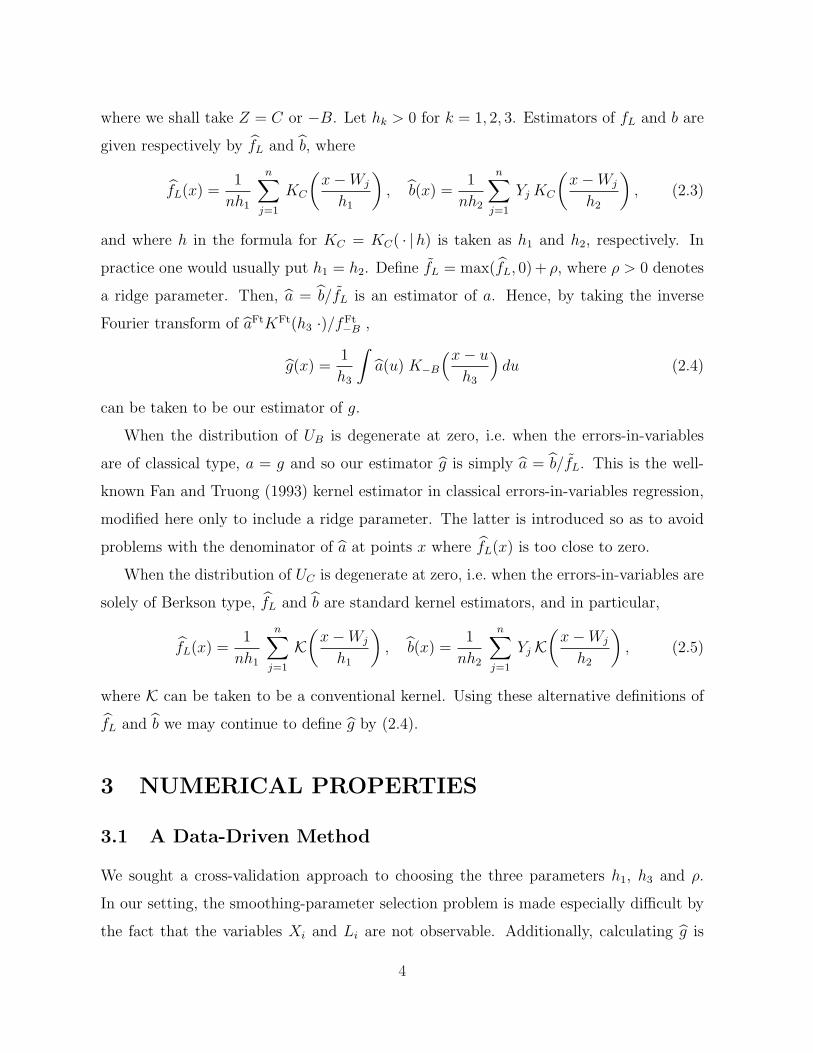
where we shall take Z = C or −B. Let hk > 0 for k = 1, 2, 3. Estimators of fL and b are
given respectively by fL and b, where
fL(x) =1
nh1
n∑j=1
KC
(x−Wj
h1
), b(x) =
1
nh2
n∑j=1
Yj KC
(x−Wj
h2
), (2.3)
and where h in the formula for KC = KC( · |h) is taken as h1 and h2, respectively. In
practice one would usually put h1 = h2. Define fL = max(fL, 0) + ρ, where ρ > 0 denotes
a ridge parameter. Then, a = b/fL is an estimator of a. Hence, by taking the inverse
Fourier transform of aFtKFt(h3 ·)/fFt−B ,
g(x) =1
h3
∫a(u) K−B
(x− u
h3
)du (2.4)
can be taken to be our estimator of g.
When the distribution of UB is degenerate at zero, i.e. when the errors-in-variables
are of classical type, a = g and so our estimator g is simply a = b/fL. This is the well-
known Fan and Truong (1993) kernel estimator in classical errors-in-variables regression,
modified here only to include a ridge parameter. The latter is introduced so as to avoid
problems with the denominator of a at points x where fL(x) is too close to zero.
When the distribution of UC is degenerate at zero, i.e. when the errors-in-variables are
solely of Berkson type, fL and b are standard kernel estimators, and in particular,
fL(x) =1
nh1
n∑j=1
K(
x−Wj
h1
), b(x) =
1
nh2
n∑j=1
Yj K(
x−Wj
h2
), (2.5)
where K can be taken to be a conventional kernel. Using these alternative definitions of
fL and b we may continue to define g by (2.4).
3 NUMERICAL PROPERTIES
3.1 A Data-Driven Method
We sought a cross-validation approach to choosing the three parameters h1, h3 and ρ.
In our setting, the smoothing-parameter selection problem is made especially difficult by
the fact that the variables Xi and Li are not observable. Additionally, calculating g is
4
a computationally intensive operation. We split the problem into two parts, selecting
(h1, ρ) and h3 separately, as follows.
Define
Sk1(`) = KC
(`−Wk
h1
)/{ n∑
k′=1
KC
(`−Wk′
h1
)+ ρ
},
Sk2(x) = h−13
∫Sk1(`) K−B
(x− `
h3
)d` .
Ideally we would use a cross-validation (CV) approach, selecting (h1, ρ) as
(h1, ρ) = argmin(h1,ρ)
n∑j=1
{Yj − a(Lj)
1− Sj1(Lj)
}2
, (3.1)
and then estimating h3 by
h3 = argminh3
n∑j=1
{Yj − g(Xj)
1− n−1∑n
k=1 Sk2(Xk)
}2
. (3.2)
(Here we use a GCV procedure in order to reduce computational labour.) However, Lj
and Xj are unobservable, and so we cannot calculate Sk1(Lj), a(Lj), Sk2(Xj) and g(Xj)
directly. We suggest two ways of estimating the unknown quantities, and combine the
two ideas to define our final procedure.
The first approach, motivated by the case where the error variances are small, is to sim-
ply ignore all error present in the data, i.e. replace all Lj’s and Xj’s by Wj’s, and replace
fFtB and fFt
C (in the definitions of KC and K−B) by 1. The second possibility is to replace
e−itLj/h1 (respectively, e−itXj/h3) in KC{(Lj −Wk)/h1} (respectively, K−B{(Xj − `)/h3})by e−itWj/h1KFt(t) / fFt
C (t/h1) (respectively, e−itWj/h3fFtB (−t/h3)/f
FtC (−t/h3)), which has,
asymptotically, the same expected value.
To gain more intuition, let (Z, f, r, V, h) denote (C, a, 1, L, h1) or (−B, g, 2, X, h3).
Then the νth procedure, ν = 1, 2, just described amounts to replacing Skr(Vj) by Skr;ν(Wj),
this being the version of Skr(Vj) obtained by replacing KZ{(Vj−·)/h} by KZ,ν{(Wj−·)/h},and f(Vj) by fν(Wj) =
∑nk=1 Yk Skr;ν(Wj), where KZ,1{(Wj − ·)/h} = K{(Wj − ·)/h},
K−B,2{(Wj − `)/h3} = KC{(Wj − `)/h3} and
KC,2
(Wj −Wk
h1
)= (2π)−1
∫exp{−it (Wj −Wk)/h1} KFt(t)
fFtC (t/h1)2
dt .
5
We noticed in our simulations that the first procedure tended to select smoothing
parameters that were too small, while the second tended to select too large values. The
following approach combines the two approaches in a way which tends to remove this
problem. (1) Choose
(h1, ρ) = argmin(h1,ρ)
n∑j=1
{w1
Yj − a1(Wj)
1− Sj1;1(Wj)+ w2
Yj − a2(Wj)
1− Sj1;2(Wj)
}2
;
then, (2) with w2 = 0.8 log{1+0.695 (σZ/σL)0.2} and w1 = 1−w2, where σ2Z is the variance
of UZ , for Z = B or C, and σ2L = σ2
W − σ2C with σ2
W the empirical variance of W , put
h3 = argminh3
n∑j=1
{w1
Yj − g1(Wj)
1− n−1∑n
k=1 Sk2;1(Wk)+ w2
Yj − g2(Wj)
1− n−1∑n
k=1 Sk2;2(Wk)
}2
;
and finally, (3) select (h1, ρ, h3) = (h1, ρ, (σB/σC)2/3 h3). The weight functions w1 and w2
were chosen empirically and are such that, when the error variance tends to zero, we select
the smoothing parameters via the first procedure only, which, for errors tending to zero,
is the same as the CV procedure that would be used in the error-free case. The correction
applied to h3 at the third step of the procedure allowed us to improve the results in cases
where one of the two errors was much larger than the other one.
3.2 Simulations
We applied the kernel method by generating samples (W1, Y1), . . . , (Wn, Yn) according to
model (1.3), where the regression function g was one of the following curves: (i) g(x) =
(50x2 + 10x + 25)−1 (sharp unimodal), (ii) g(x) = φ0,1.5(4x) + φ1,2(4x) + φ2,5(4x) (asym-
metric), and (iii) g(x) = 5 sin(2x) exp(−16x2/50) (sinusoidal), where φµ,σ is the density
of an N(µ, σ2) variable.
For each example, the variable L was either a centered normal or a multiple of T8, a
Student-t distributed variable with eigth degrees of freedom, and the error variables UB
and UC were normal or Laplace variables, centered at zero and having a variance equal
to 10% and 20%, respectively, of the variance of L. The variable η was N(0, σ2η), where
σ2η = 0.1× var|g|. Here, var|g| was defined by var(|g|) =
∫ q0.99
q0.01(|g| − E|g|)2/(q0.99 − q0.01),
6

−4 −2 0 2 4
−4
−2
02
4
x
targ
etd1d5d9
−4 −2 0 2 4
−4
−2
02
4
x
targ
et
d1d5d9
−4 −2 0 2 4
−4
−2
02
4
x
targ
et
d1d5d9
−4 −2 0 2 4
−4
−2
02
4
x
targ
et
d1d5d9
−4 −2 0 2 4
−4
−2
02
4
x
targ
et
d1d5d9
−4 −2 0 2 4
−4
−2
02
4
x
targ
et
d1d5d9
Figure 1: Estimation of function (iii) for samples of size n = 250, when L ∼ √0.75 T8,
UB and UC are Laplace (row 1) or normal (row 2), when (σ2B/σ2
L, σ2C/σ2
L) is, from left to
right, (0.1, 0.1), (0.1, 0.2), (0.2, 0.2). The solid curve is the target curve.
where E(|g|) =∫ q0.99
q0.01|g|/(q0.99 − q0.01) and qα was the αth quantile of |g| rescaled to
integrate to 1.
In each case, we considered samples of size n = 100 or 250, we generated 200 replicated
samples from the random vector (W,Y ), and we constructed the corresponding estimator
g, using the data-driven method of Section 3.1 and the kernel K with Fourier transform
KFt(t) = (1−t2)3 1[−1,1](t), which is commonly used in deconvolution problems. We report
the Integrated Squared Error, ISE(x) =∫ {g(x)− g(x)}2 dx. In all figures, the estimates
shown correspond to the first (d1), fifth (d5) and ninth (d9) deciles of the ordered values
of ISE. We present only a portion of the results; the conclusions are also supported by
the simulations not presented here.
In deconvolution problems it is rather common to consider two classes of errors, called
ordinary-smooth and supersmooth errors. Roughly, an error of the first (respectively,
second) type has a characteristic function behaving like a negative polynomial (respec-
tively, exponential) in the tails. Rates of convergence in errors-in-variables problems are
7
−4 −2 0 2 4
0.00
0.01
0.02
0.03
0.04
x
targ
etd1d5d9
−4 −2 0 2 4
0.00
0.01
0.02
0.03
0.04
x
targ
et
d1d5d9
−4 −2 0 2 4
0.00
0.01
0.02
0.03
0.04
x
targ
et
d1d5d9
−4 −2 0 2 4
0.00
0.01
0.02
0.03
0.04
x
targ
et
d1d5d9
−4 −2 0 2 4
0.00
0.01
0.02
0.03
0.04
x
targ
et
d1d5d9
−4 −2 0 2 4
0.00
0.01
0.02
0.03
0.04
x
targ
et
d1d5d9
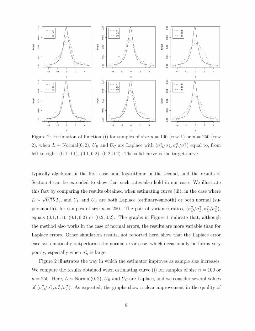
Figure 2: Estimation of function (i) for samples of size n = 100 (row 1) or n = 250 (row
2), when L ∼ Normal(0, 2), UB and UC are Laplace with (σ2B/σ2
L, σ2C/σ2
L) equal to, from
left to right, (0.1, 0.1), (0.1, 0.2), (0.2, 0.2). The solid curve is the target curve.
typically algebraic in the first case, and logarithmic in the second, and the results of
Section 4 can be extended to show that such rates also hold in our case. We illustrate
this fact by comparing the results obtained when estimating curve (iii), in the case where
L ∼ √0.75 T8, and UB and UC are both Laplace (ordinary-smooth) or both normal (su-
persmooth), for samples of size n = 250. The pair of variance ratios, (σ2B/σ2
L, σ2C/σ2
L),
equals (0.1, 0.1), (0.1, 0.2) or (0.2, 0.2). The graphs in Figure 1 indicate that, although
the method also works in the case of normal errors, the results are more variable than for
Laplace errors. Other simulation results, not reported here, show that the Laplace error
case systematically outperforms the normal error case, which occasionally performs very
poorly, especially when σ2B is large.
Figure 2 illustrates the way in which the estimator improves as sample size increases.
We compare the results obtained when estimating curve (i) for samples of size n = 100 or
n = 250. Here, L ∼ Normal(0, 2), UB and UC are Laplace, and we consider several values
of (σ2B/σ2
L, σ2C/σ2
L). As expected, the graphs show a clear improvement in the quality of
8

−2 −1 0 1 2 3
0.0
0.1
0.2
0.3
0.4
0.5
0.6
x
targ
etd1d5d9
−2 −1 0 1 2 3
0.0
0.1
0.2
0.3
0.4
0.5
0.6
x
targ
et
d1d5d9
−2 −1 0 1 2 3
0.0
0.1
0.2
0.3
0.4
0.5
0.6
x
targ
et
d1d5d9
−2 −1 0 1 2 3
0.0
0.1
0.2
0.3
0.4
0.5
0.6
x
targ
et
d1d5d9
−2 −1 0 1 2 3
0.0
0.1
0.2
0.3
0.4
0.5
0.6
x
targ
et
d1d5d9
−2 −1 0 1 2 3
0.0
0.1
0.2
0.3
0.4
0.5
0.6
x
targ
et
d1d5d9
Figure 3: Estimation of function (ii) for samples of size n = 250, when L ∼ Normal(0, 1),
UB is Laplace and UC is normal, with (σ2B/σ2
L, σ2C/σ2
L) equal to, from left to right, (0.1, 0.1),
(0.1, 0.2), (0.2, 0.1). Row 1 shows the estimator (2.4) and row 2 shows the local linear
estimator that ignores the error in the data. The solid curve is the target curve.
the estimators, in all cases, as n increases from 100 to 250.
Figure 3 illustrates the performance of the estimator in a case where the classical error
is smoother than the Berkson error — a situation encountered very often in real-data
applications. We compare the results obtained when estimating curve (ii) for different
values of (σ2B/σ2
L, σ2C/σ2
L), when the classical error UC is normal, i.e. supersmooth, and the
Berkson error UB is Laplace, i.e. ordinary-smooth. Here, L ∼ Normal(0, 1) and the 200
generated samples are of size n = 250. Here, and also in all other cases we considered, the
best results are clearly in the case of the lowest error variance, i.e. σ2B = σ2
C = 0.1σ2L. In
the figure we also illustrate the effect of the errors present in the data; we show the local-
linear estimators obtained when ignoring the error, i.e. when using the procedure with
plug-in bandwidth described by Fan and Gijbels (1995). The graphs show that ignoring
the error leads to severely biased estimators.
Of course, as for any nonparametric method in the usual ‘error-free’ regression prob-
9

−4 −2 0 2 4
−4
−2
02
4
x
targ
etd1d5d9
−4 −2 0 2 4
−4
−2
02
4
x
targ
et
d1d5d9
−4 −2 0 2 4
−4
−2
02
4
x
targ
et
d1d5d9
Figure 4: Estimation of function (iii) when n = 250, L ∼ Normal(0, σ2L) and Z ∼ Laplace
(√
0.5 σZ), with Z = UB or UC , for (σ2L, σ2
B, σ2C) equal to, from left to right, (0.5, 0.05, 0.1),
(1, 0.1, 0.2) or (2, 0.2, 0.4). The solid curve is the target curve.
lem, the quality of the estimator also depends on the range of the observed sample. In
particular, for a given family of densities fB, fC and fL, and given noise-to-signal ratios
σ2B/σ2
L and σ2C/σ2
L, the performance of the estimator depends on the variance of UB, UC
and L. For example, Figure 4 illustrates the results of estimating regression function
(iii) in the case where n = 250, L ∼ Normal(0, σ2L) and Z ∼ Laplace (
√0.5 σZ), with
Z = UB or UC , for (σ2L, σ2
B, σ2C) = (0.5, 0.05, 0.1), (1, 0.1, 0.2) or (2, 0.2, 0.4). When the
variances are smaller, the observations are more concentrated around the centre, and, as
a consequence, it is easier to recover the peaks of the curve. As the variances increase the
observations become more widespread, and, for a given sample size, it becomes harder to
recover the peaks of the regression curve, since the peaks are located around the centre
zero.
Finally, we apply our method to a case where the function g is unbounded. We take
g(x) = x2, L ∼ N(0, 1) and UB and UC are Laplace, with σ2B = σ2
C = 0.1. Here, since |g|integrates to infinity, we alter the definition of q0.01 and q0.99 in E|g| and var|g|, and take
q0.99 = −q0.01 = 2.5, corresponding approximately to the 0.99 quantile of the distribution
of L. In Section 4.3 we shall show that, although it seems quite hard to deal with such
unbounded functions g, our estimator is able to estimate g on a compact interval, of length
growing with the sample size. In Figure 5, we illustrate these results by showing the decile
curves obtained for samples of size n = 100, 250 and 500. We see clearly that, as the
sample size increases, the estimator is able to estimate g correctly on growing intervals.
10

−2 0 2
02
46
x
targ
et
d1d5d9
−2 0 2
02
46
x
targ
et
d1d5d9
−2 0 2
02
46
x
targ
et
d1d5d9
Figure 5: Estimation of the curve g(x) = x2 when L ∼ Normal(0, 1) and Z ∼ Laplace
(√
0.05), with Z = UB or UC and sample size is, from left to right, n = 100, 250 or 500.
The solid curve is the target curve.
Note that we show the estimated curves over a relatively large range, since the interval
[−2.5, 2.5] contains L with a probability of 0.988.
3.3 Data Example
We applied the kernel method to data from the Nevada Test Site (NTS) Thyroid Disease
Study; see, for example, Stevens et al. (1992), Kerber et al. (1993) and Simon et al. (1995).
The goal of the study was to relate radiation exposure (largely due to above-ground
nuclear testing in the 1950s) to various thyroid disease outcomes. In the Nevada study,
over 2, 000 individuals exposed to radiation as children were examined for thyroid disease.
The primary radiation exposure came from milk and vegetables. A recent update of the
dosimetry is available (Simon et al. 2005), as is a reanalysis of the thyroid disease data
(Lyon et al. 2006). We analyze a subset of the revised dosimetry data, namely the 1,278
women in the study, 103 of whom developed thyroiditis.
In this example, X (resp., W ) is the logarithm of the true (resp., observed) radiation
exposure and Y = 0 or 1 indicates absence or presence of thyroid disease. As discussed
in Mallick, et al. (2002), the uncertainties in this problem are a mixture of classical and
Berkson measurement errors. Following the illustrative analysis of Mallick et al. (2002), in
this illustration we assume that 50% of the total uncertainty variance is classical, and 50%
is Berkson. Also, as in their analysis and those of many others in the area, the Berkson
and classical uncertainties in the log-scale are assumed to be normally distributed.
11

x−axisy−
axis
−7 −6 −5 −4 −3 −2
0.06
0.08
0.10
Figure 6: Estimation of the regression curve for the thyroid data in the log-scale. The
x-axis is the logarithm of true dose, while the y-axis is the estimated risk of thyroiditis.
We applied our estimation procedure on these data, with smoothing parameters se-
lected via the method described in Section 3.1, with the kernel K as in Section 3.2. The
estimator of the regression curve P (Y = 1|X = x) is shown at Figure 6, for values of
x in the range [−7,−1.5], which corresponds to the values between the 10th and 90th
percentiles of the sample of observed log-doses. The graph shows a continuous, roughly
quadratic increase in risk as the true log-doses of radiation increase. Our results are
roughly in accord with the parametric analysis of Lyon, et al. (2006), although their use
of an excess relative risk model is less flexible than ours.
4 THEORETICAL PROPERTIES
4.1 Discussion of case of unbounded g
In the simple error-free case (i.e. the case where UB ≡ UC ≡ 0), nonparametric estimation
of an unbounded regression curve g defined on the whole real line is a hard problem:
in finite samples, the observations are confined to a finite range and in general, only
the observations in the neighborhood of the point x where we want to estimate g bring
valuable information about the value of g(x). Hence, unless g(x) → 0 as x → ∞, it is
usually not possible to construct a good estimator of g outside the range of the observed
data.
One of the interesting aspects of errors-in-variables problems is that nonparametric
12

inference cannot be undertaken in a strictly local sense. In particular, to estimate g at
x it is not adequate to rely on noisy observations of g at points close to x; observations
of g across its support are used to estimate g at a point in the middle of the support.
However, especially when the errors are of Berkson type, use of data on an unbounded,
infinitely supported function g can involve significant challenges: in finite samples, it is
impossible to observe values of L over more than just a finite range, and hence to obtain
information across the whole support of g.
Consider, for example, the case where g is unbounded and the distribution of the errors
UB has unbounded support. Specifically, assume that the proxy variable L is compactly
supported; that the Berkson error UB has a Laplace distribution, P (|UB| > x) = e−x for
x > 0; and that g(x) = ex2. Because the tails of the distribution of UB decrease more
slowly than the tails of g increase, then with high probability, any sample of data on
Y = g(L + UB) + η contains many very large values. In particular, for each D1 > 0 and
D2 ∈ (0, 1), the probability that g(Lj + UB,j) + ηj > nD1 for at least nD2 values of j in
the range 1 ≤ j ≤ n, converges to 1 as n →∞. In such instances, the observations on Y
are too ‘volatile’ and the estimator can turn out to be extremely unstable.
Circumstances as extreme as this are awkward to accommodate. One way of avoiding
this type of difficulty is to restrict attention to the case of bounded g, but that prevents
us from treating relatively standard cases such as, for example, polynomial g. Although
the problem can be very hard, we show below that our estimator can in fact be used
for such unbounded g; moreover, and perhaps surprisingly, the only way in which our
estimator is affected by the fact that, in finite samples, we can only observe data on L
over a finite range, is that we can only guarantee consistent estimation of g over a finite,
but growing with n, interval. We shall prove consistency of g by exploiting its similarities
with gn, the estimator of the function gn, which we define as the restriction of g over a
finite, but growing, interval. In situations less extreme than the one mentioned in the
previous paragraph, g and gn are sufficiently close for asymptotic properties of g to be
derivable from those of gn. More precisely, we assume that:
the distribution of UB has all moments finite, and |g(x)| ≤ D3 xD4 for all x,
where D3, D4 > 0 are constants,(4.1)
13

and we define gn = g · 1[−nD5 ,nD5 ](x), where, for a set A, 1A(x) = 1 if x ∈ A and 0
otherwise. If R is any compact set, then it can be proved from (4.1) that,
for any D5 > 0, no matter how small, P{gn(x) = g(x) for all x ∈ R}
=
1−O(n−D6) for any D6 > 0, no matter how large.(4.2)
Provided (4.1) holds, for any given D7 > 0, no matter how small, we can, by choosing
D5 > 0 sufficiently small, ensure that,
sup |gn| = O(nD7
)and
∫|gn| = O
(nD7
). (4.3)
We will see at the end of Subsection 4.3 that, together, (4.1)–(4.3) permit us to deal
with the case of unbounded, infinitely supported g by working with its truncated version
gn. This approach motivates the assumption, influencing (4.4) below, that g may depend
on n.
The assumption in (4.1) that all moments are finite is satisfied by the most common
error distributions. The condition |g(x)| = O(xD4) asks only that g increase no more than
polynomially fast, which is a mild constraint.
4.2 Notation and Assumptions
Motivated by the arguments in Subsection 4.1, we shall permit g = gn to depend on n,
subject to satisfying:
max
(sup |g|,
∫|g|
)≤ λ = λ(n) , (4.4)
where λ ≥ 1. It follows that a and b, at (2.1) and (2.3), can also depend on n, although
to avoid sub-subscripts we do not express this in notation. We adopt a conventional,
fixed-function interpretation of fB, fC , fL and the distribution of η.
Biases for the estimators fL and b, defined at (2.3), are respectively given by
biasf (x) = E{fL(x)− fL(x)} =1
2π
∫fFt
L (t){KFt(h1t)− 1
}e−itx dt ,
biasb(x) = E{b(x)− b(x)} =1
2π
∫bFt(t)
{KFt(h2t)− 1
}e−itx dt .
14

Define too
biasg(x) =1
2π
∫gFt(t)
{KFt(h3t)− 1
}e−itx dt ,
it being assumed in each case that the integral is convergent in the Riemann sense. To
interpret biasg, consider the case where g is a probability density, and we observe noisy
data generated as ζ = ηg + η, where ηg has density g, and η is independent of ηg and has
a known distribution with a characteristic function that does not vanish on the real line.
Then, biasg represents the bias of the standard deconvolution kernel estimator of g with
bandwidth h3.
Taking, for simplicity, h1 = h2, let supbi(h1) denote the maximum of the suprema of
the biases biasb and biasf , and define also δ, closely related to root mean squared error:
supbi(h1) = maxc=b,f
sup−∞<x<∞
|biasc(x)| , δ = λ−1 supbi(h1) + (nh2α+11 )−1/2 ,
where λ is as at (4.4) and α > 1 will be determined by (4.6); let R denote a finite union
of compact intervals on which fL is bounded away from zero; and assume that
(a) fL is uniformly bounded; (b) there exists an open set S containing R,
such that fL is bounded away from zero on S; and (c) for a constant ξ ∈(0,∞], fL(x) ≥ C1 (1 + |x|)−ξ for all |x|.
(4.5)
We permit ξ = ∞ in (4.5), in which case (4.5)(c) is degenerate and only (4.5)(a) and
(4.5)(b) are effective.
Next we state assumptions about the known densities fC and fB, the kernel K and
the regression mean g; see (4.6)(a)–(d), respectively. With C2 > 0 denoting a constant
and bβc the integer part of β, our assumptions are:
for constants α, β, γ such that α, β > 1 and β + γ ≥ 1 is an integer,
(a) |(d/dt)j fFtC (st)−1| ≤ C2 sj (1 + st)α−j, for j = 0 and 1, all |t| ≤ 1 and all
s ≥ 1; (b) |(d/dt)j fFt−B(st)−1| ≤ C2 sj (1 + st)β−j when 0 ≤ j ≤ min(β, β+
γ + 1), and |(d/dt)j fFt−B(st)−1| ≤ C2 sbβc when min(β, β + γ + 1) < j ≤
max(β, β + γ + 1), for all |t| ≤ 1 and all s ≥ 1; (c) |(d/dt)j KFt(t)| ≤ C2 for
0 ≤ j ≤ β + γ + 1 and for all t, and KFt(0) = 1 and KFt(t) vanishes outside
[−1, 1]; and (d) g satisfies (4.4).
(4.6)
15

The conditions imposed on fC and fB are a variation of the assumptions |fFtC (t)| ≥
const. (1+ |t|)−α and |fFt−B(t)| ≥ const. (1+ |t|)−β, respectively, which are typically encoun-
tered in errors-in-variables problems. They apply if, for example, the error distributions
are of Laplace type, and in particular if fC = φ( · |α) and fB = φ( · | β), where φ( · |ω) is
the density of the distribution function with characteristic function (1 + t2)−ω for all t.
Then, (a) holds with α = 2ω > 1, and (b) holds with β = 2ω and γ depending on ω.
More particularly, the case where fFt−B is the inverse of a polynomial, which occurs if, for
example, fFt−B(t) = (1 + t2)−ω and ω is an integer, is of special interest. More generally,
suppose that
fFt−B(t)−1 = 1 +
p∑j=1
cj tj , (4.7)
where 2 ≤ p < ∞ and the cj’s are constants. Then, it is readily checked that (4.6)(b)
holds. Smoother types of errors, for example those with Fourier transform bounded below
by a negative exponential, can be considered as well. Results similar to those given in
Section 4.3 hold for such errors too, but with considerably slower convergence rates. See
the discussion at the end of Section 4.3.
The restriction imposed on K reflects the fact that the compact support of KFt can
be taken, without loss of generality, to be contained in [−1, 1], and asks as well that KFt
be sufficiently smooth. In practice it is common to define K by KFt(t) = (1 − tr1)r2 for
t ∈ [−1, 1], and KFt = 0 otherwise, where r1 is an even integer and r2 is a positive integer.
In such cases, (4.6)(c) holds provided
r2 > β + γ + 1 (4.8)
and the value of γ is limited only by the size of r2; γ does not depend on selection of
the constants p and c1, . . . , cp in (4.7). In particular, by choosing r2 sufficiently large we
can take γ arbitrarily large in (4.6). These considerations generally permit us to take
ξ = ∞ in (4.5)(c); see the discussion immediately below Theorem 4.1. In such cases, (4.5)
imposes especially mild conditions on fL.
More generally, (4.5) and (4.6), and the statement of our main results in Section 4.3,
are tailored to permit relatively weak conditions on fL and g. For example, no smoothness
16

assumptions are imposed at this point. Indeed, we shall raise the smoothness issue only
through the bias terms biasb, biasf and biasg.
4.3 Properties in the Mixed Error Case
Here we assume the model (1.3), when neither of the errors UC and UB has a degenerate
distribution. The estimator g is given by (2.4), with fL and b defined at (2.3). For
simplicity we omit the case β + γ = ξ in (4.9) below; it is the same as for β + γ < ξ,
except that a factor log n is included. Upper bounds to convergence rates are given below.
We do not have minimax lower bounds that reflect the upper bounds.
Theorem 4.1. If (4.5) and (4.6) hold, and if h1 = h2 and 0 < h1, h3 ≤ B1 where B1 > 0,
then, for a constant B2 > 0 not depending on n, h1, h2 or h3,
supx∈R
E∣∣∣g(x)− g(x)− biasg(x)
∣∣∣ ≤ B2 λ(ρ + δ + ρ−1 δ2
)h−β
3
×
(1 + hβ+γ
3 ρ(β+γ)/ξ−1)
if β + γ < ξ(1 + hβ+γ
3
)if β + γ > ξ ,
(4.9)
where λ is as at (4.4).
To interpret this theorem, let us first consider the case where g is a bounded, integrable
function. Then the contribution of g to bias is represented in (4.9) by
biasg(x) =
∫K(u) {g(x− h3u)− g(x)} du = O
(hk
3
), (4.10)
where the first identity holds under the conditions of Theorem 4.1, and the second identity
holds provided g has k bounded derivatives,∫
(1 + |u|)k |K(u)| du < ∞ , (4.11)
and κj =∫
uj K(u) du = 0 for j = 1, . . . , k−1. Kernels satisfying these conditions, as well
as those in (4.6)(c), are commonly used in practice. For example, the kernels employed
in Section 3 are of this type for k = 2.
Bias formulae such as (4.10) are of course conventional. It is the remaining contribution
to convergence rate, bounded by the right-hand side of (4.9), that is most affected by the
17

errors-in-variables aspect of the problem and is therefore of greatest interest. Take the
ridge parameter ρ to equal a constant multiple of δ and assume that we can choose γ,
in (4.6), so large that hγ3 = O(ρ) (this assumption is not an issue if f−B satisfies (4.7).
Related interpretations of (4.9) are also possible where the simplifications obtainable when
f−B is given by (4.7) do not apply, but those instances are not so transparent, since then
both γ and ξ can impact on the overall convergence rate). Then (4.9) further simplifies to:
supx∈R
E∣∣∣g(x)− g(x)− biasg(x)
∣∣∣ = O(λ δ h−β
3
), (4.12)
where, since g is bounded and integrable, λ can be taken constant and so can be omitted
from (4.12). Results (4.10) and (4.12) imply the following rate of convergence of g to g:
supx∈R
E|g(x)− g(x)| = O(hk
3 + δ h−β3
). (4.13)
If fL has k bounded derivatives, then δ ∼ const. × n−k/(2α+2k+1) provided we take
h1 ∼ const. n−1/(2α+2k+1). This order of δ is also the minimax-optimal, root squared-
error convergence rate for estimators of g, in the case where UB is identically zero. See,
for example, Fan and Truong (1993). Thus, the factor h−β3 , on the right-hand side of
(4.13), can be interpreted as the amount by which the conventional convergence rate, δ,
is degraded by introducing the additional error UB.
Of course, the factor h−β3 diverges as the bandwidth h3 becomes smaller. On the other
hand, the bias term hk3 reduces to zero as h3 decreases, so there will be an optimal order
of magnitude of h3 for which the contributions hk3 and δ h−β
3 are in balance, leading to:
supx∈R
E|g(x)− g(x)| = O(n−k2/{(2α+2k+1)(β+k)}
). (4.14)
Result (4.9) reveals the potential deleterious effects of taking the ridge, ρ, too large
(that is, of larger order than δ) or too small. In particular, the order of magnitude of the
right-hand side of (4.9) is made larger by choosing ρ to be of either strictly larger order,
or strictly smaller order, than δ.
It is straightforward to combine Theorem 4.1, and the results in Section 4.1, to handle
the case of fixed but unbounded g. Specifically, taking gn = g · 1[−nD,nD](x), with D > 0
18

arbitrarily small, and assuming that (4.1) holds, (4.2) permits us to take λ = O(nr) for
any r > 0 in (4.9), provided we replace biasg(x) there by,
biasgn(x) =
∫K(u) {gn(x− h3u)− gn(x)} du = O
(nshk
3
)(4.15)
for all s > 0. The second identity in (4.15) holds provided g(k)n exists and |g(k)
n | grows no
more than polynomially fast, κj = 0 for j = 1, . . . , k − 1, and, in a mild strengthening
of (4.11),∫ |u|k+c |K(u)| du < ∞ for some c > 0. Therefore, and using also (4.12), the
following version of (4.14) follows from (4.2) and (4.9): For all r > 0,
supx∈R
|g(x)− g(x)| = Op
(n−(k2−r)/{(2α+2k+1)(β+k)}
). (4.16)
Thus it can be seen that unboundeness of g barely changes the convergence rate.
Note too from (4.14) and (4.16) that our bounds on the rate of convergence increase as
the smoothness of either error distribution increases; that is, as α or β increases. These
results correctly suggest that if either of the errors were “supersmooth,” for example
Gaussian, the convergence rate would be slower than the inverse of any polynomial in n.
In fact, no estimator can converge at a polynomial rate in the supersmooth cases.
5 ORTHOGONAL SERIES METHOD
An alternative estimator of g can be considered in the case where g, fB and fL are
compactly supported. Here and below, we assume that fL, g and fB have been rescaled
so that all three support intervals are contained within I = [−π, π]. In this case, it follows
from work of Delaigle, Hall and Qiu (2006) that no nonparametric estimator can identify g
outside the interval [aL +aB, bL−aB], where [−aB, aB] and [aL, bL] denote the supports of,
respectively, fB and fL. Here, for simplicity, we have assumed that fB is symmetric. The
estimator we describe below is able to identify g on the interval [aL+aB, bL−aB], whatever
the support, compact or not, of the classical error density fC . The trigonometric-series
expansion of a function k with support contained in I may be written as,
k(x) = k0 +∞∑
j=1
{k1j cos(jx) + k2j sin(jx)} ,
19

with k0 = (2π)−1∫I k and, for ` = 1, 2, k`,j = π−1
∫I k(x) cs`,j(x) dx, where cs`,j(x) =
cos(jx) or sin(jx) according as ` = 1 or 2, respectively. Using the sine-cosine decomposi-
tion of g and a, we have, from Delaigle, Hall and Qiu (2006)
(c1j
c2j
)=
1
δ21j + δ2
2j
(δ1j δ2j
−δ2j δ1j
)(r1j
r2j
), (5.1)
where, for ` = 1, 2, (c`,j, δ`,j, r`,j) denotes (g`,j, α`,j, a`,j), with α`,j = E{cs`,j(UB)} , and
an estimator of the Fourier coefficients of g can be deduced from (5.1), by replacing the
Fourier coefficients a0 and a`,j by a0 = (2π)−1∫I a and a`,j = π−1
∫I a cs`,j, where we
choose a to be a sine-cosine series estimator of a, defined by borrowing ideas of Hall and
Qiu (2005) in the context of pure classical errors.
More precisely, define b = a fL, p`,j = π−1E{cs`,j(W )} and q`,j ≡ π−1E{Y cs`,j(W )},for ` = 1, 2. Then it can be shown that (5.1) holds with (c`,j, δ`,j, r`,j) equal to either
(fL`,j, β`,j, p`,j) or (b`,j, β`,j, q`,j), where β`,j = E{cs`,j(UC)}, ` = 1, 2. Substituting the
estimators p`,j = (πn)−1∑
i cs`,j(Wi) and q`,j = (πn)−1∑
i Yi cs`,j(Wi) for p`,j and q`,j,
we see that a can be estimated by
a(x) =b0 +
∑j≥1 {b1j cos(jx) + b2j sin(jx)}
(2π)−1 +∑
j≥1 {fL1jcos(jx) + fL2j
sin(jx)}.
In practice, we need to truncate the series for a and only keep the terms corresponding to
j ≤ M1, where, for example, M1 can be chosen by a thresholding rule as in Hall and Qiu
(2005). The series for g needs also be truncated, to keep only the terms j ≤ M2, where
M2 can be selected by a cross-validation procedure of the type introduced in Delaigle,
Hall and Qiu (2006).
6 OUTLINE PROOF OF THEOREM 4.1
Define fL = max(fL, 0), ∆b = b− b, ∆f = fL − fL, ∆f = fL − fL, kx(u) = h−13 K−B{(u−
x)/h3} and Q1 = 2 (|a|∆2f + |∆b ∆f |)/{ρ (fL + ρ)}. It can be shown that,
g(x)− g(x) = biasg(x)− ρ
∫a kx
fL + ρ+ Ab(x)− Af (x) + Q2(x) , (6.1)
20

where
Ab(x) =
∫∆b kx
fL + ρ, Af (x) =
∫b ∆f kx
(fL + ρ)2, |Q2(x)| ≤
∫Q1 |kx| . (6.2)
Using (b) and (c) of (4.6) it can be shown that |K−B(x |h)| ≤ C1 h−β (1 + |x|)−(β+γ+1)
for all real x and all h > 0, where C1, C2, . . . will denote positive constants. This leads
to the result, hβ3
∫ |kx| (fL + ρ)−1 ≤ C2 (I1 + I2), where, with C > 0 chosen so small
that x + h3u ∈ S whenever x ∈ R and |h3u| ≤ C, and R and S as in (4.5), we define
I1 =∫|h3u|≤C
(1 + |u|)−(β+γ+1) du ≤ C3,
I2 =
∫
|h3u|>C
{(h3|u|)−ξ + ρ
}−1(1 + |u|)−(β+γ+1) du ≤ C4
hβ+γ3 ρ(β+γ)/ξ−1 if β + γ < ξ
hβ+γ3 if β + γ > ξ .
Combining the results in this paragraph we deduce that
hβ3
∫ |kx|fL + ρ
≤ C5
(1 + hβ+γ
3 ρ(β+γ)/ξ−1)
if β + γ < ξ(1 + hβ+γ
3
)if β + γ > ξ ,
(6.3)
uniformly in x ∈ R.
Using (4.6)(a) and the definition of supbi(h1) it can be shown that, for c = b and
c = f , we have, uniformly in x,
E{∆b(u)2
}+ |a|2E{
∆f (u)2} ≤ C6 λ2 δ2 . (6.4)
Using (6.3), (6.4) and the result |b| ≤ C7 λ fL, it can be proved that, for c = b and c = f ,
{EAc(x)2
}1/2 ≤ C8 λ δ h−β3
(1 + hβ+γ
3 ρ(β+γ)/ξ−1)
if β + γ < ξ(1 + hβ+γ
3
)if β + γ > ξ ,
(6.5)
ρ
∣∣∣∣∫
a kx
fL + ρ
∣∣∣∣ ≤ C9 λ ρ h−β3
(1 + hβ+γ
3 ρ(β+γ)/ξ−1)
if β + γ < ξ(1 + hβ+γ
3
)if β + γ > ξ ,
(6.6)
where both formulae hold uniformly in x ∈ R. Together, (6.1), (6.5) and (6.6) give:
g(x)− g(x) = biasg(x) + Q2(x) + Q3(x) , (6.7)
21

where Q2 is as before, and so satisfies the last inequality at (6.2), and
{EQ3(x)2
}1/2 ≤ C10 λ (ρ + δ) h−β3
(1 + hβ+γ
3 ρ(β+γ)/ξ−1)
if β + γ < ξ(1 + hβ+γ
3
)if β + γ > ξ ,
(6.8)
uniformly in x ∈ R. Properties (6.3) and (6.4), and the last inequality at (6.2), entail:
E|Q2(x)| ≤ C11 λ δ2 ρ−1 h−β3
(1 + hβ+γ
3 ρ(β+γ)/ξ−1)
if β + γ < ξ(1 + hβ+γ
3
)if β + γ > ξ .
(6.9)
Results (6.7)–(6.9) imply that g(x)−g(x) = biasg(x)+Q4(x), where, uniformly in x ∈ R,
E|Q4(x)| ≤ C12 λ{ρ + δ + δ2 ρ−1}h−β
3
(1 + hβ+γ
3 ρ(β+γ)/ξ−1)
if β + γ < ξ(1 + hβ+γ
3
)if β + γ > ξ .
Theorem 4.1 follows directly from these properties.
Acknowledgments
Carroll’s research was supported by a grant from the National Cancer Institute, and
by the Texas A&M Center for Environmental and Rural Health via a grant from the
National Institute of Environmental Health Sciences. Delaigle’s research was supported
by a Hellman Fellowship and a Maurice Belz Fellowship. We thank Dr. J. Lynn Lyon for
giving us access to the Nevada Test Site data and Dr. F. Owen Hoffman for many helpful
discussions on the mixture of Berkson and classical uncertainties.
REFERENCES
Berkson, J. (1950). Are there two regression problems? J. Amer. Statist. Assoc. 45,
164–180.
Buonaccorsi, J. P. and Lin, C.-D. (2002). Berkson measurement error in designed repeated
measures studies with random coefficients. J. Statist. Plann. Inf. 104, 53-72.
Carroll, R. J., Maca, J. D. and Ruppert, D. (1999). Nonparametric regression in the
presence of measurement error. Biometrika 86, 541–554.
22

Carroll, R. J., Ruppert, D., Stefanski, L. A. and Crainiceanu, C. M. (2006). Measurement
Error in Nonlinear Models, second edition. Chapman and Hall CRC Press, Boca
Raton.
Cook, J. R. and Stefanski, L. A. (1994). Simulation-extrapolation estimation in paramet-
ric measurement error models. J. Amer. Statist. Assoc. 89, 1314–1328.
Delaigle, A. (2007). Nonparametric density estimation from data contaminated by Berk-
son errors, classical errors, or a mixture of both. Can. J. Statist., 35, 1–16.
Delaigle, A., Hall, P. and Qiu, P. (2006). Nonparametric methods for solving the Berkson
errors-in-variables problem. J. Roy. Statist. Soc., B 68, 201–220.
Devanarayan, V. and Stefanski, L. A. (2002). Empirical simulation extrapolation for
measurement error models with replicate measurements. Statist. Probab. Lett.
59, 219-225.
Fan, J. and Gijbels, I. (1996). Local Polynomial Modelling and Its Applications, Chapman
and Hall: London.
Fan, J. and Masry, E. (1992). Multivariate regression estimation with errors-in-variables:
asymptotic normality for mixing processes. J. Multivariate Anal. 43, 237–271.
Fan, J. and Truong, Y. K. (1993). Nonparametric regression with errors in variables.
Ann. Statist. 21, 1900–1925.
Hall, P. and Qiu, P. (2005). Discrete-transform approach to deconvolution problems.
Biometrika 92, 135–148.
Huwang, L. and Huang, H. Y. S. (2000). On errors-in-variables in polynomial regression
– Berkson case. Statist. Sinica 10, 923-936.
Kerber, R. L., Till, J. E., Simon, S. L., Lyon, J. L. Thomas, D. C., Preston-Martin, S.,
Rollison, M. L., Lloyd, R. D. and Stevens, W. (1993). A cohort study of thyroid
disease in relation to fallout from nuclear weapons testing. J. Amer. Medical
Assoc. 270, 2076-2083.
Kim, J. and Gleser, L. J. (2000). SIMEX approaches to measurement error in ROC
studies. Comm. Statist. Theory Meth. 29, 2473–2491.
Li, Y., Guolo, A., Hoffman, F. O. and Carroll, R. J. (2007). Shared uncertainty in
measurement error problems, with application to Nevada Test Site Fallout data.
Biometrics, to appear.
Linton, O. and Whang, Y. J. (2002). Nonparametric estimation with aggregated data.
Econometric Theory 18, 420–468.
Lyon, J. L., Alder, S. C., Stone, M. B., Scholl, A., Reading, J. C. Holubkov, R., Sheng,
X., White, G. L., Hegmann, K. T., Anspaugh, L., Hoffman, F. O., Simon, S. L.,
Thomas, B., Carroll, R. J. and Meikle, A. W. (2006). Thyroid disease associ-
ated with exposure to the Nevada Test Site radiation: a reevaluation based on
corrected dosimetry and examination data. Epidemiology 17, 604-614.
Mallick, B., Hoffman, F. O. and Carroll, R. J. (2002). Semiparametric regression modeling
23

with mixtures of Berkson and classical error, with application to fallout from the
Nevada test site. Biometrics 58, 13-20.
Reeves, G. K., Cox, D. R., Darby, S. C. and Whitley, E. (1998). Some aspects of measure-
ment error in explanatory variables for continuous and binary regression models.
Stat. Medicine 17, 2157-2177.
Schafer, D. W. and Gilbert, E. S. (2006). Some statistical implications of dose uncertainty
in radiation dose-response analyses. Radiation Research 166, 303-312.
Simon, S. L., Till, J. E., Lloyd, R. D., Kerber, R. L., Thomas, D. C., Preston-martin,
S., Lyon, J. L. and Stevens, W. (1995). The Utah Leukemia case-control study:
dosimetry methodology and results. Health Physics 68, 460-471.
Simon, S. L., Anspaugh, L. R., Hoffman, F. O., et al. (2006). Update of dosimetry for
the Utah Thyroid Cohort Study. Radiation Research 165, 208-22.
Stefanski, L. A. and Cook, J. R. (1995). Simulation-extrapolation: The measurement
error jackknife. J. Amer. Statist. Assoc. 90, 1247–1256.
Stevens, W., Till, J. E., Thomas, D. C., et al. (1992). Assessment of leukemia and thyroid
disease in relation to fallout in Utah: report of a cohort study of thyroid disease
and radioactive fallout from the Nevada test site. University of Utah.
Stram, D. O., Huberman, M. and Wu, A. H. (2002). Is residual confounding a reason-
able explanation for the apparent protective effects of beta-carotene found in
epidemiological studies of lung cancer in smokers? Amer. J. Epidemiol. 155,
622–628.
Taupin, M. L. (2001). Semi-parametric estimation in the nonlinear structural errors-in-
variables model. Ann. Statist. 29, 66–93.
Wang, L. (2003). Estimation of nonlinear Berkson-type measurement error models.
Statist. Sinica 13, 1201–1210.
24

NOT-FOR-PUBLICATION APPENDIX: DETAILS FOR
SECTION 6
Put fL = max(fL, 0), ∆b = b− b, ∆f = fL − fL and ∆f = fL − fL, and observe that
1
fL + ρ=
1
fL + ρ− ∆f
(fL + ρ)(fL + ρ).
Therefore,
b + ∆b
fL + ρ=
b + ∆b
fL + ρ− b ∆f
(fL + ρ)2+
b ∆2f
(fL + ρ)2(fL + ρ)− ∆b ∆f
(fL + ρ)(fL + ρ).
Also,b
fL
− b
fL + ρ=
ρ b
fL (fL + ρ)=
ρ a
fL + ρ,
and sob + ∆b
fL + ρ=
b
fL
− ρ a
fL + ρ+
∆b
fL + ρ− b ∆f
(fL + ρ)2+ Q1 ,
where Q1, denoting quadratic terms, satisfies
|Q1| ≤|a| ∆2
f + |∆b ∆f |(fL + ρ)(fL + ρ)
≤ |a|∆2f + |∆b ∆f |
ρ (fL + ρ). (A.1)
Here we have used the fact that |∆f | ≤ |∆f |.Now, |∆f − ∆f | = |fL| I(fL < 0) ≤ |∆f | I(fL < 0), from which result and (A.1) it
follows that
b + ∆b
fL + ρ=
b
fL
− ρ a
fL + ρ+
∆b
fL + ρ− b ∆f
(fL + ρ)2+ Q2 , (A.2)
where Q2 satisfies:
|Q2| ≤|a|∆2
f + |∆b ∆f |ρ (fL + ρ)
+|b ∆f | I(fL < 0)
(fL + ρ)2. (A.3)
However, if fL < 0 then |∆f | > fL, whence it follows that
|b ∆f | I(fL < 0)
(fL + ρ)2≤ |b|∆2
f
fL (fL + ρ)2=
|a|∆2f
(fL + ρ)2.
Hence, (A.3) implies that
|Q2| ≤ Q3 ≡ 2|a|∆2
f + |∆b ∆f |ρ (fL + ρ)
. (A.4)
25
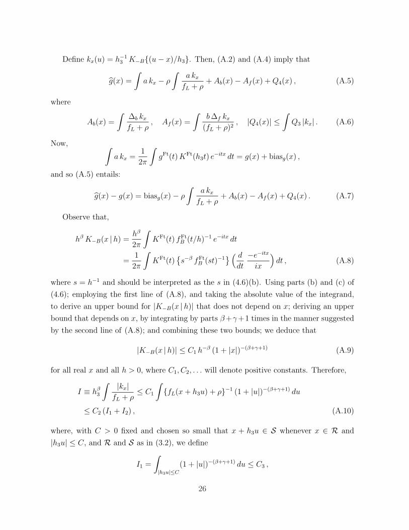
Define kx(u) = h−13 K−B{(u− x)/h3}. Then, (A.2) and (A.4) imply that
g(x) =
∫a kx − ρ
∫a kx
fL + ρ+ Ab(x)− Af (x) + Q4(x) , (A.5)
where
Ab(x) =
∫∆b kx
fL + ρ, Af (x) =
∫b ∆f kx
(fL + ρ)2, |Q4(x)| ≤
∫Q3 |kx| . (A.6)
Now, ∫a kx =
1
2π
∫gFt(t) KFt(h3t) e−itx dt = g(x) + biasg(x) ,
and so (A.5) entails:
g(x)− g(x) = biasg(x)− ρ
∫a kx
fL + ρ+ Ab(x)− Af (x) + Q4(x) . (A.7)
Observe that,
hβ K−B(x |h) =hβ
2π
∫KFt(t) fFt
B (t/h)−1 e−itx dt
=1
2π
∫KFt(t)
{s−β fFt
B (st)−1} ( d
dt
−e−itx
ix
)dt , (A.8)
where s = h−1 and should be interpreted as the s in (4.6)(b). Using parts (b) and (c) of
(4.6); employing the first line of (A.8), and taking the absolute value of the integrand,
to derive an upper bound for |K−B(x |h)| that does not depend on x; deriving an upper
bound that depends on x, by integrating by parts β +γ +1 times in the manner suggested
by the second line of (A.8); and combining these two bounds; we deduce that
|K−B(x |h)| ≤ C1 h−β (1 + |x|)−(β+γ+1) (A.9)
for all real x and all h > 0, where C1, C2, . . . will denote positive constants. Therefore,
I ≡ hβ3
∫ |kx|fL + ρ
≤ C1
∫{fL(x + h3u) + ρ}−1 (1 + |u|)−(β+γ+1) du
≤ C2 (I1 + I2) , (A.10)
where, with C > 0 fixed and chosen so small that x + h3u ∈ S whenever x ∈ R and
|h3u| ≤ C, and R and S as in (3.2), we define
I1 =
∫
|h3u|≤C
(1 + |u|)−(β+γ+1) du ≤ C3 ,
26
I2 =
∫
|h3u|>C
{(h3|u|)−ξ + ρ
}−1(1 + |u|)−(β+γ+1) du
≤ C4
{∫ h−13 ρ−1/ξ
Ch−13
(h3u)ξ
(1 + u)β+γ+1du + ρ−1
∫ ∞
h−13 ρ−1/ξ
(1 + |u|)−(β+γ+1) du
}
≤ C5
hβ+γ3 ρ(β+γ)/ξ−1 if β + γ < ξ
hβ+γ3 if β + γ > ξ
+ C5 ρ−1(h3 ρ1/ξ
)β+γ
≤ C6
hβ+γ3 ρ(β+γ)/ξ−1 if β + γ < ξ
hβ+γ3 if β + γ > ξ .
Here we have used the fact that fL(u) ≥ |u|−ξ for all sufficiently large |u|. Combining the
results from (A.10) down we deduce that
hβ3
∫ |kx|fL + ρ
≤ C7
(1 + hβ+γ
3 ρ(β+γ)/ξ−1)
if β + γ < ξ(1 + hβ+γ
3
)if β + γ > ξ ,
(A.11)
uniformly in x ∈ R.
Analogously to (A.9) it can be shown using (4.6)(a) that for all x and all h > 0,
|KC(x |h)| ≤ C8 h−α1 (1 + |x|)−1 . (A.12)
It follows from the definition of supbi(h1) that max(|E∆b|, |E∆f |) ≤ supbi(h1). Using
(A.12) to obtain the second inequality below, it can be proved that, uniformly in u,
var{∆f (u)} ≤ 1
nh21
∫KC
(u− w
h1
)2
fW (w) dw ≤ C9
(nh2α+1
1
)−1. (A.13)
An identical bound applies to var{∆b(u)}, although with a factor λ2; recall the assumption
that var(η) < ∞, imposed as part of model (1.3). Combining the results so far in this
paragraph we deduce that, for c = b and c = f , we have, uniformly in u,
E{∆b(u)2
}+ |a|2E{
∆f (u)2} ≤ C10 λ2 δ2 . (A.14)
The function fB, being a density, is integrable, and hence, in view of (2.1), the function
a is bounded above by a constant multiple of λ. Hence, by (2.2), |b| ≤ C11 λ fL for a
constant C11 > 0. This property, (A.11) and (A.14) together imply that, for c = b and
c = f ,
{EAc(x)2
}1/2 ≤ C12 λ δ h−β3
(1 + hβ+γ
3 ρ(β+γ)/ξ−1)
if β + γ < ξ(1 + hβ+γ
3
)if β + γ > ξ .
(A.15)
27

Formula (A.11) also implies that
ρ
∣∣∣∣∫
a kx
fL + ρ
∣∣∣∣ ≤ C13 λ ρ h−β3
(1 + hβ+γ
3 ρ(β+γ)/ξ−1)
if β + γ < ξ(1 + hβ+γ
3
)if β + γ > ξ ,
(A.16)
where both (A.15) and (A.16) hold uniformly in x ∈ R. Together, (A.7), (A.15) and
(A.16) give:
g(x)− g(x) = biasg(x) + Q4(x) + Q5(x) , (A.17)
where Q4 is as before, and so satisfies the last inequality at (A.6), and
{EQ5(x)2
}1/2 ≤ C14 λ (ρ + δ) h−β3
(1 + hβ+γ
3 ρ(β+γ)/ξ−1)
if β + γ < ξ(1 + hβ+γ
3
)if β + γ > ξ ,
(A.18)
uniformly in x ∈ R.
Properties (A.4), (A.11) and (A.14), and the last inequality at (A.6), entail:
E|Q4(x)| ≤∫
E(Q3) |kx|
≤ C15 λ δ2 ρ−1 h−β3
(1 + hβ+γ
3 ρ(β+γ)/ξ−1)
if β + γ < ξ(1 + hβ+γ
3
)if β + γ > ξ .
(A.19)
Combining (A.17)–(A.19) we deduce that
g(x)− g(x) = biasg(x) + Q6(x) , (A.20)
where, uniformly in x ∈ R,
E|Q6(x)| ≤ C16 λ{ρ + δ + δ2 ρ−1
}h−β
3
(1 + hβ+γ
3 ρ(β+γ)/ξ−1)
if β + γ < ξ(1 + hβ+γ
3
)if β + γ > ξ .
(A.21)
Theorem 4.1 follows directly from (A.20) and (A.21).
28
Related Documents