UNIVERSIDAD POLITÉCNICA DE MADRID Escuela Técnica Superior de Ingenieros de Telecomunicación NONPARAMETRIC MESSAGE PASSING METHODS FOR COOPERATIVE LOCALIZATION AND TRACKING Ph.D. Thesis Tesis Doctoral Vladimir Savić Ingeniero de Electrónica 2012

Welcome message from author
This document is posted to help you gain knowledge. Please leave a comment to let me know what you think about it! Share it to your friends and learn new things together.
Transcript
UNIVERSIDAD POLITÉCNICA DE MADRIDEscuela Técnica Superior de Ingenieros de
Telecomunicación
NONPARAMETRIC MESSAGE PASSINGMETHODS FOR COOPERATIVE
LOCALIZATION AND TRACKING
Ph.D. ThesisTesis Doctoral
Vladimir SavićIngeniero de Electrónica
2012

DEPARTAMENTO DE SEÑALES, SISTEMAS YRADIOCOMUNICACIONES
Escuela Técnica Superior de Ingenieros de Telecomunicación
Universidad Politécnica de Madrid
NONPARAMETRIC MESSAGE PASSINGMETHODS FOR COOPERATIVE
LOCALIZATION AND TRACKING
TESIS DOCTORAL
Autor:
Vladimir SavićIngeniero de Electrónica
Director:
Santiago Zazo BelloProfesor titular del Dpto. de Señales, Sistemas y Radiocomunicaciones
Universidad Politécnica de Madrid
2012

TESIS DOCTORAL
NONPARAMETRIC MESSAGE PASSING METHODS FORCOOPERATIVE LOCALIZATION AND TRACKING
AUTOR: Vladimir SavićDIRECTOR: Santiago Zazo Bello
Tribunal nombrado por el Mgfco. y Excmo. Sr. Rector de la UniversidadPolitécnica de Madrid, el día de de 2012.
PRESIDENTE: Narciso García Santos
SECRETARIO: Jesús Grajal de la Fuente
VOCAL: Antonio Artés Rodríguez
VOCAL: Joaquín Míguez Arenas
VOCAL: Lennart Svensson
SUPLENTE: Tomas McKelvey
SUPLENTE: Jesús Pérez Arriaga
Realizado el acto de defensa y lectura de Tesis el día de de 2012.
En la E.T.S. de Ingenieros de Telecomunicación.
Calificación:
EL PRESIDENTE LOS VOCALES
EL SECRETARIO


To my family


Acknowledgements
This Ph.D thesis would not have been possible without the support of many people.First of all, I would like to thank my supervisor Santiago Zazo Bello for his helpand many useful advices. I also appreciate that he gave me a chance to participatein many international conferences, and to perform a part of my research at anotheruniversities.
Furthermore, I would like to thank Petar M. Djurić (Stony Brook University) forsupervising me during my visit, and for providing me the access to the laboratory. Ialso thank Akshay Athalye (Stony Brook University), and Miodrag Bolić (Universityof Ottawa) for useful advices, and their support for performing the experiments.
Many thanks to Henk Wymeersch (Chalmers University) and Federico Penna(Politecnico di Torino) for their collaboration, which resulted in the novel algorithmuseful for many applications, including the topic of this thesis. Moreover, I thankHenk Wymeersch for supervising me during my visit at Chalmers University. I alsothank Lennart Svensson (Chalmers University) for the useful proposals on how toreduce the complexity of the proposed algorithms.
Many thanks to my colleagues at “Grupo de Aplicaciones de Procesado de Señal”(GAPS), especially Adrián Población, Benjamin Béjar, Igor Arambasić, Ivana Raos,Mariano García, Nelson Dopico, Pavle Belanović, Sergio Valcarcel. Moreover, Ithank to colleague from “Grupo de Microondas y Radar” (GMR), Ángel GarcíaFernández. I especially appreciate their advices that improved my research results,and their help to solve some administrative problems.
I would like to thank Bernard Henri Fleury (Aalborg University), Jesús Grajal(Universidad Politecnica de Madrid) and Ronald Raulefs (German Aerospace Center- DLR) for taking their time to review my thesis.
Finally, I also thank my family and all friends. Special thanks to my parents,Jovan and Olga, for their enormous support during my stay in Spain.
ix

x
Abstract
The objective of this thesis is the development of cooperative localization and track-ing algorithms using nonparametric message passing techniques. In contrast to themost well-known techniques, the goal is to estimate the posterior probability dens-ity function (PDF) of the position of each sensor. This problem can be solvedusing Bayesian approach, but it is intractable in general case. Nevertheless, theparticle-based approximation (via nonparametric representation), and an appropri-ate factorization of the joint PDFs (using message passing methods), make Bayesianapproach acceptable for inference in sensor networks. The well-known method forthis problem, nonparametric belief propagation (NBP), can lead to inaccurate be-liefs and possible non-convergence in loopy networks. Therefore, we propose fournovel algorithms which alleviate these problems: nonparametric generalized beliefpropagation (NGBP) based on junction tree (NGBP-JT), NGBP based on pseudo-junction tree (NGBP-PJT), NBP based on spanning trees (NBP-ST), and uniformly-reweighted NBP (URW-NBP). We also extend NBP for cooperative localization inmobile networks. In contrast to the previous methods, we use an optional smoothing,provide a novel communication protocol, and increase the efficiency of the samplingtechniques. Moreover, we propose novel algorithms for distributed tracking, in whichthe goal is to track the passive object which cannot locate itself. In particular, wedevelop distributed particle filtering (DPF) based on three asynchronous belief con-sensus (BC) algorithms: standard belief consensus (SBC), broadcast gossip (BG),and belief propagation (BP). Finally, the last part of this thesis includes the ex-perimental analysis of some of the proposed algorithms, in which we found thatthe results based on real measurements are very similar with the results based ontheoretical models.
xi

xii
Resumen
El objetivo de esta tesis es el desarrollo de los algoritmos para posicionamiento yseguimiento cooperativo mediante técnicas no paramétricas de paso de mensajes. Encontraste con la mayoría de técnicas bien conocidas, el objetivo es estimar la fun-ción densidad de probabilidad posterior de la posición de cada sensor. Este problemase puede resolver mediante técnica bayesiana, pero es insoluble en el caso general.Sin embargo, se puede resolver utilizando la aproximación basada en partículas (através de la representación no paramétrica), y una factorización apropiada de las fun-ciones densidad de probabilidad conjunta (utilizando métodos de paso de mensajes).Método bien conocido para este problema, nonparametric belief propagation (NBP),puede causar certezas inexactas y posible falta de convergencia en las redes conbucles. Por lo tanto, proponemos cuatro nuevos algoritmos que pueden resolver estosproblemas: nonparametric generalized belief propagation (NGBP) basado en junctiontree (NGBP-JT), NGBP basado en pseudo-junction tree (NGBP-PJT), NBP basadoen spanning trees (NBP-ST), y uniformly-reweighted NBP (URW-NBP). Tambiénproponemos extension de NBP para posicionamiento cooperativo en redes móviles.En contraste con los métodos anteriores, enviamos un mensaje opcional desde el fu-turo al presente, proponemos el nuevo protocolo para comunicación, y aumentamoseficaz de técnicas de muestreo. Además, proponemos nuevos algoritmos para elseguimiento distributivo, en el que el objetivo es realizar el seguimiento del objetopasivo que no puede ubicarse. En particular, desarrollomos filtros de particulas dis-tributivas (DPF) basados en tres belief consensus (BC) algoritmos: standard beliefconsensus (SBC), broadcast gossip (BG), y belief propagation (BP). Finalmente, laúltima parte de esta tesis incluye el análisis experimental de algunos de los algorit-mos propuestos, en el que se encontró que los resultados basados en medidas realesson muy similares a los resultados basados en modelos teóricos.
xiii

xiv
Contents
1 Introduction 1
1.1 Thesis objectives . . . . . . . . . . . . . . . . . . . . . . . . . . . . . 1
1.2 Outline of the thesis . . . . . . . . . . . . . . . . . . . . . . . . . . . 2
1.3 List of publications . . . . . . . . . . . . . . . . . . . . . . . . . . . . 3
2 Overview of cooperative localization techniques 5
2.1 Introduction . . . . . . . . . . . . . . . . . . . . . . . . . . . . . . . . 5
2.1.1 Motivating applications . . . . . . . . . . . . . . . . . . . . . 6
2.1.2 Classification of cooperative localization methods . . . . . . . 7
2.2 Measurement techniques . . . . . . . . . . . . . . . . . . . . . . . . . 9
2.2.1 Received signal strength (RSS) . . . . . . . . . . . . . . . . . 9
2.2.2 Time of arrival (TOA) . . . . . . . . . . . . . . . . . . . . . . 10
2.2.3 Time difference of arrival (TDOA) . . . . . . . . . . . . . . . 11
2.2.4 Lighthouse approach . . . . . . . . . . . . . . . . . . . . . . . 12
2.2.5 Angle of arrival (AOA) . . . . . . . . . . . . . . . . . . . . . 13
2.2.6 RSS profiling technique . . . . . . . . . . . . . . . . . . . . . 15
2.3 Deterministic localization techniques . . . . . . . . . . . . . . . . . . 16
2.3.1 Connectivity based algorithms . . . . . . . . . . . . . . . . . 16
2.3.2 Distance based algorithms . . . . . . . . . . . . . . . . . . . . 23
2.3.3 Localization using AOA . . . . . . . . . . . . . . . . . . . . . 31
2.4 Probabilistic localization techniques . . . . . . . . . . . . . . . . . . 34
2.5 Summary . . . . . . . . . . . . . . . . . . . . . . . . . . . . . . . . . 35
3 Message passing methods for cooperative localization in loopy net-
xv
works 37
3.1 Introduction . . . . . . . . . . . . . . . . . . . . . . . . . . . . . . . . 37
3.2 Belief propagation (BP) . . . . . . . . . . . . . . . . . . . . . . . . . 38
3.3 Nonparametric belief propagation (NBP) . . . . . . . . . . . . . . . 41
3.3.1 Computing messages . . . . . . . . . . . . . . . . . . . . . . . 42
3.3.2 Computing beliefs . . . . . . . . . . . . . . . . . . . . . . . . 43
3.3.3 Convergence of NBP . . . . . . . . . . . . . . . . . . . . . . . 44
3.3.4 Nonparametric boxed belief propagation (NBBP) . . . . . . . 44
3.3.5 Simulation results . . . . . . . . . . . . . . . . . . . . . . . . 45
3.3.6 Comparison with MDS . . . . . . . . . . . . . . . . . . . . . . 47
3.4 Correctness of BP . . . . . . . . . . . . . . . . . . . . . . . . . . . . 48
3.5 Generalized belief propagation (GBP) methods . . . . . . . . . . . . 50
3.5.1 GBP based on Kikuchi approximation (GBP-K) . . . . . . . 50
3.5.2 GBP based on junction-tree (GBP-JT) . . . . . . . . . . . . 51
3.5.3 GBP based on pseudo-junction-tree (GBP-PJT) . . . . . . . 52
3.5.4 Nonparametric approximation of GBP-PJT method . . . . . 58
3.5.5 Simulation results . . . . . . . . . . . . . . . . . . . . . . . . 64
3.6 Nonparametric belief propagation based on spanning trees (NBP-ST) 68
3.6.1 ST formation . . . . . . . . . . . . . . . . . . . . . . . . . . . 69
3.6.2 Simulation results . . . . . . . . . . . . . . . . . . . . . . . . 71
3.7 Uniformly-reweighted nonparametric belief propagation (URW-NBP) 72
3.7.1 Edge appearance probabilities . . . . . . . . . . . . . . . . . . 74
3.7.2 Simulation results . . . . . . . . . . . . . . . . . . . . . . . . 74
3.8 Summary . . . . . . . . . . . . . . . . . . . . . . . . . . . . . . . . . 79
4 Cooperative mobile network localization and tracking 81
4.1 Introduction . . . . . . . . . . . . . . . . . . . . . . . . . . . . . . . . 81
4.2 Cooperative localization in mobile networks . . . . . . . . . . . . . . 82
4.2.1 Extension of NBP for mobile networks . . . . . . . . . . . . . 83
4.2.2 A novel communication protocol . . . . . . . . . . . . . . . . 86
4.2.3 Improving sampling techniques . . . . . . . . . . . . . . . . . 88
4.2.4 Simulation results . . . . . . . . . . . . . . . . . . . . . . . . 92
xvi
4.3 Distributed target tracking . . . . . . . . . . . . . . . . . . . . . . . 98
4.3.1 Overview of centralized target tracking . . . . . . . . . . . . . 99
4.3.2 Distributed particle filtering . . . . . . . . . . . . . . . . . . . 102
4.3.3 Belief consensus algorithms . . . . . . . . . . . . . . . . . . . 103
4.3.4 Simulation results . . . . . . . . . . . . . . . . . . . . . . . . 108
4.4 Summary . . . . . . . . . . . . . . . . . . . . . . . . . . . . . . . . . 113
5 Experimental study of cooperative localization and tracking meth-ods 115
5.1 Introduction . . . . . . . . . . . . . . . . . . . . . . . . . . . . . . . . 115
5.2 Experimental study of NBP and NBP-ST methods . . . . . . . . . . 116
5.2.1 Experimental setup . . . . . . . . . . . . . . . . . . . . . . . . 116
5.2.2 Indoor modeling using RSS measurements . . . . . . . . . . . 117
5.2.3 Simulation results . . . . . . . . . . . . . . . . . . . . . . . . 120
5.3 Localization and tracking using novel RFID system . . . . . . . . . . 122
5.3.1 A novel sensatag-based RFID system . . . . . . . . . . . . . . 123
5.3.2 Sensatag localization . . . . . . . . . . . . . . . . . . . . . . . 125
5.3.3 Sensatag tracking . . . . . . . . . . . . . . . . . . . . . . . . . 127
5.3.4 Experimental results . . . . . . . . . . . . . . . . . . . . . . . 130
5.4 Summary . . . . . . . . . . . . . . . . . . . . . . . . . . . . . . . . . 137
6 Conclusions and future work 139
6.1 Conslusions . . . . . . . . . . . . . . . . . . . . . . . . . . . . . . . . 139
6.2 Future work . . . . . . . . . . . . . . . . . . . . . . . . . . . . . . . . 140
A GBP-JT: example network 143
B Convergence behavior of BP consensus 147
C Sensatag-based RFID localization 149
C.1 Functional blocks of the sensatag . . . . . . . . . . . . . . . . . . . . 149
C.2 Potential applications . . . . . . . . . . . . . . . . . . . . . . . . . . 151
Bibliography 155
xvii

xviii
List of Figures
2.1 (a) Single-hop and (b) multi-hop (cooperative) localization. . . . . . 6
2.2 Illustration of lighthouse approach . . . . . . . . . . . . . . . . . . . 13
2.3 Typical anisotropic antenna . . . . . . . . . . . . . . . . . . . . . . . 14
2.4 An antenna array with N antenna elements . . . . . . . . . . . . . . 15
2.5 DV-hop correction example . . . . . . . . . . . . . . . . . . . . . . . 18
2.6 Anchor beacon transmission ranges for (a) CAB-EA, and (b) CAB-EW 21
2.7 Example of localization using CAB . . . . . . . . . . . . . . . . . . . 23
2.8 Single-hop and 2-hop examples. . . . . . . . . . . . . . . . . . . . . . 25
2.9 N-hop scenario: (a) regular, and (b) irregular case . . . . . . . . . . 26
2.10 Initial estimates for node C . . . . . . . . . . . . . . . . . . . . . . . 26
2.11 The graph obtained after running the fold-free phase . . . . . . . . . 30
2.12 Nodes with AOA capability . . . . . . . . . . . . . . . . . . . . . . . 32
2.13 Illustration of AOA algorithm . . . . . . . . . . . . . . . . . . . . . . 33
3.1 Example of pairwise potential. . . . . . . . . . . . . . . . . . . . . . 39
3.2 An example of 5 node network and belief of node 5 . . . . . . . . . . 40
3.3 An example of 5 node network and belief of node 5 (information from2-hop neighbors included). . . . . . . . . . . . . . . . . . . . . . . . . 40
3.4 Drawing particles within the box. . . . . . . . . . . . . . . . . . . . . 45
3.5 Comparison of the results for a 50-node network (a) NBP, (b) NBBP. 45
3.6 Comparison of the (a) accuracy and (b) coverage . . . . . . . . . . . 46
3.7 Comparison of the (a) computational and (b) communication cost . 46
3.8 Comparison between NBBP and MDS . . . . . . . . . . . . . . . . . 48
3.9 (a) A simple loopy network, (b) Corresponding unwrapped networkfor the first 3 iterations . . . . . . . . . . . . . . . . . . . . . . . . . 49
xix
3.10 The basic clusters in the (a) Bethe approximation and (b) Kikuchiapproximation . . . . . . . . . . . . . . . . . . . . . . . . . . . . . . 50
3.11 (a) Triangulated 6-node graph, and corresponding (b) cluster graph,(c) clique tree, and (d) JT. . . . . . . . . . . . . . . . . . . . . . . . 53
3.12 (a) Example of 10-node graph, and (b) corresponding TG. . . . . . . 57
3.13 (a) Cluster graph based on TG from Figure 3.12b, and (b) corres-ponding PJT. . . . . . . . . . . . . . . . . . . . . . . . . . . . . . . . 57
3.14 Illustration of initial particles from 2-node and 3-node cliques. . . . . 60
3.15 Illustration of results for the 60-node network: (a) NBP, (b) NBP-TG,and (c) NGBP-PJT. . . . . . . . . . . . . . . . . . . . . . . . . . . . 63
3.16 Comparison of NBP, NBP-TG and NGBP-PJT beliefs. . . . . . . . . 65
3.17 CDF of RMSE. . . . . . . . . . . . . . . . . . . . . . . . . . . . . . . 66
3.18 The effect of transmission radius on RMSE in position . . . . . . . . 66
3.19 Comparison of KL divergence in each iteration . . . . . . . . . . . . 67
3.20 Communication cost for PJT formation . . . . . . . . . . . . . . . . 68
3.21 The effect of transmission radius on communication cost. . . . . . . 69
3.22 Original network with 100 unknown nodes and two corresponding STs. 71
3.23 Comparison of (a) accuracy and (b) coverage . . . . . . . . . . . . . 72
3.24 Comparison of (a) computational and (b) communication cost . . . . 72
3.25 (a) 4-node clique, and (b) 16 STs. . . . . . . . . . . . . . . . . . . . . 75
3.26 Optimum ρ estimation in 4-node network. . . . . . . . . . . . . . . . 75
3.27 NBP, TRW-NBP (ρ = 0.5), and true belief for the one of the targetnodes (x = 0m). . . . . . . . . . . . . . . . . . . . . . . . . . . . . . 76
3.28 Grid topology: (a) RMSE for different transmission radius, (b) Em-pirical model for optimal ρ. . . . . . . . . . . . . . . . . . . . . . . . 77
3.29 Random topology: (a) RMSE for different transmission radius, (b)Empirical model for optimal ρ. . . . . . . . . . . . . . . . . . . . . . 77
3.30 Comparison of the error for: (a) R = 6.6m, and (b) R = 16m. . . . . 78
4.1 Example of a graphical model for mobile positioning. . . . . . . . . . 83
4.2 Possible positions of target nodes in the case of (a) MIS, and (b)MIS-RP. . . . . . . . . . . . . . . . . . . . . . . . . . . . . . . . . . . 89
4.3 Tracking 5 nodes using different variants of NBP. . . . . . . . . . . . 93
xx
4.4 Comparison of the RMSE for: (a) grid, and (b) semi-random topolo-gies of the anchor nodes. . . . . . . . . . . . . . . . . . . . . . . . . . 93
4.5 KLD between approximated belief and particle-based belief. . . . . . 94
4.6 CDF of the position error for different approximations. . . . . . . . . 95
4.7 Comparison between MIS and MIS-RP . . . . . . . . . . . . . . . . . 96
4.8 Comparison between NBP, PMC-NBP and ANBP methods. . . . . . 97
4.9 Illustration of target tracking in a WSN. . . . . . . . . . . . . . . . . 100
4.10 Example of track in 25-node network. . . . . . . . . . . . . . . . . . 109
4.11 Determination of consensus parameters. . . . . . . . . . . . . . . . . 109
4.12 Performance comparison of DPF methods as a function of the numberof iterations. . . . . . . . . . . . . . . . . . . . . . . . . . . . . . . . 111
4.13 Performance comparison of DPF and CPF/NCPF as a function ofcommunication radius. . . . . . . . . . . . . . . . . . . . . . . . . . . 112
4.14 Communication cost comparison as a function of the communicationradius. . . . . . . . . . . . . . . . . . . . . . . . . . . . . . . . . . . . 113
5.1 (a) Crossbow’s IRIS wireless sensor node, (b) Illustration of the ex-periment in our lab. . . . . . . . . . . . . . . . . . . . . . . . . . . . 117
5.2 Illustration of (a) path-loss exponent estimation, and (b) reliablemodel for distance estimation . . . . . . . . . . . . . . . . . . . . . . 118
5.3 Histogram of distance estimate. . . . . . . . . . . . . . . . . . . . . . 119
5.4 Estimated probability of detection . . . . . . . . . . . . . . . . . . . 119
5.5 Examples of the pairwise potential functions . . . . . . . . . . . . . . 120
5.6 (a) Original network, (b),(c) two corresponding STs. . . . . . . . . . 121
5.7 Comparison of (a) accuracy, and (b) coverage. . . . . . . . . . . . . . 121
5.8 Comparison of (a) computational cost, and (b) communication cost. 122
5.9 Received Signal Strength (RSS) (from reader) at sensatag . . . . . . 124
5.10 Architecture of the sensatag-based RFID system. . . . . . . . . . . . 124
5.11 Sensing zone of the sensatag . . . . . . . . . . . . . . . . . . . . . . . 125
5.12 Experimental setup for sensatag localization . . . . . . . . . . . . . . 131
5.13 The effect of reader power on the average position error. . . . . . . . 132
5.14 Estimated probability of detection and the corresponding four-degreepolynomial fitting. . . . . . . . . . . . . . . . . . . . . . . . . . . . . 132
xxi
5.15 CDF of position error. . . . . . . . . . . . . . . . . . . . . . . . . . . 133
5.16 CDF of position error in different scenarios . . . . . . . . . . . . . . 133
5.17 CDF of position error for LOS and three NLOS scenarios. . . . . . . 134
5.18 Experimental setup for sensatag tracking. . . . . . . . . . . . . . . . 134
5.19 Illustration of results of tracking for two different tracks. . . . . . . . 135
5.20 Comparison of the (a) RMSEs, and (b) CDFs of position errors. . . . 136
5.21 Performance comparison of PF-BIN and DPF-BIN methods . . . . . 137
A.1 Example of triangulated 10-node network. . . . . . . . . . . . . . . . 144
A.2 The junction tree corresponding to the network in Figure A.1 . . . . 145
B.1 Example graphs for BP consensus . . . . . . . . . . . . . . . . . . . 148
C.1 Block diagram of the sensatag. . . . . . . . . . . . . . . . . . . . . . 150
C.2 Sensatag board used in the experiments . . . . . . . . . . . . . . . . 150
C.3 Experimental setup for typical warehouse application. . . . . . . . . 152
C.4 Binomial distribution for all 3 classes, and corresponding decisionbounds. . . . . . . . . . . . . . . . . . . . . . . . . . . . . . . . . . . 154
xxii

List of Acronyms
AFL Anchor-free localization
ANBP Auxiliary nonparametric belief propagation
AOA Angle of arrival
APF Auxiliary particle filtering
BC Belief consensus
BFS Breadth first search
BG Broadcast gossip
BP Belief propagation
CAB Concentric anchor beacon
CDF Cumulative distribution function
CPF Centralized particle filtering
DOM Direction of movement
DPF Distributed particle filtering
DV Distance-vector
GBP Generalized belief propagation
GPS Global positioning system
JT Junction tree
KDE Kernel density estimate
KF Kalman filter
KLD Kullback-Leibler (KL) divergence
xxiii

LOS Line-of-sight
MAP Maximum a posteriori
MC Max-consensus
MDS Multi-dimensional scaling
MIS Mixture importance sampling
ML Maximum likelihood
MMSE Minimum mean square estimate
NBBP Nonparametric boxed belief propagation
NBP Nonparametric belief propagation
NCPF Non-centralized particle filtering
NGBP Nonparametric generalized belief propagation
NLOS Non-line-of-sight
PDF Probability density function
PF Particle filtering
PJT Pseudo-junction tree
PMC Population Monte Carlo
RFID Radio-frequency identification
RIP Running intersection property
RMSE Root-mean-square (RMS) error
RP Reference particles
RSS Received signal strength
SBC Standard belief consensus
SIR Sample-importance-resampling
ST Spanning tree
TDOA Time difference of arrival
TG Thin graph
xxiv

TOA Time of arrival
TRW Tree-reweighted
UHF Ultra-high frequency
URW Uniformly-reweighted
UWB Ultra-wide band
WC Weighted centroid
WLAN Wireless local area networks
WSN Wireless sensor network
xxv

xxvi
Chapter 1
Introduction
1.1 Thesis objectives
In this thesis, we develop novel cooperative localization and tracking algorithms, forstatic and mobile networks, using nonparametric message passing techniques. Incontrast to the most well-known techniques, the goal is to estimate posterior prob-ability density function (PDF) of the position of each sensor. This problem canbe solved using Bayesian approach, but it is intractable in general case. Neverthe-less, the particle-based approximation (via nonparametric representation), and anappropriate factorization of the joint PDFs (using message passing methods), makeBayesian approach acceptable for inference in sensor networks. Extensions of well-known method for this problem, nonparametric belief propagation (NBP), are themain topic of this thesis. There are four main objectives:
• Development of novel message passing methods for cooperative localization inloopy networks. The goal is to improve performance of standard NBP, whichcan lead to inaccurate beliefs and possible non-convergence in loopy networks.
• Development of novel NBP-based algorithms for cooperative localization inmobile networks. The goal is to use smoothing nearly in real time, decreasethe communication cost, and increase the efficiency of sampling techniques.
• Development of novel belief consensus methods for distributed tracking of thepassive object. The goal is to use fastest consensus method, and to allow theuse of all parametric and nonparametric likelihood functions.
• Experimental analysis in indoor environment of some of the proposed al-gorithms for static and mobile networks. To that end, we use IRIS wirelessmotes, and semi-passive Radio-Frequency IDentification (RFID) system.
1
Introduction
1.2 Outline of the thesis
The rest of this thesis is organized as follows:
• Chapter 2 reviews cooperative (multi-hop) localization techniques, in whichsmall number of sensors, called anchor nodes, obtain their coordinates viaGlobal positioning system (GPS) or by installing them at points with knowncoordinates, and the rest, unknown nodes, must determine their own coordin-ates using the anchor’s positions and measured inter-sensor distances. Sincethe sensors are usually energy-conserving devices, i.e., without energy neces-sary for long-range communication, they have available only the noisy meas-urements of the distance to several neighboring nodes. In particular, we de-scribe standard measurement techniques, deterministic localization methods(distance-based and connectivity-based), localization using angle of arrival(AOA), and general framework for probabilistic localization.
• Chapter 3 addresses static positioning using improved message passing meth-ods. We first describe and analyse standard techniques, BP and NBP. Then,we propose nonparametric boxed belief propagation (NBBP), in which we ad-ded the bounded boxes to constraint the area from which the particles aredrawn. Since all of these methods (BP, NBP, NBBP) can lead to inaccuratebeliefs and possible non-convergence in loopy networks, we propose four im-proved message-passing methods: nonparametric generalized belief propaga-tion (NGBP) based on junction tree (NGBP-JT), NGBP based on pseudo-junction tree (NGBP-PJT), NBP based on spanning trees (NBP-ST), anduniformly-reweighted NBP (URW-NBP).
• Chapter 4 addresses two important problems: cooperative localization in mo-bile networks, and distributed tracking of the passive object. For the firstproblem, we extend NBP described in Chapter 3. In contrast to previousmethods, we send optional message from the future to present using only 1-legsmoothing, and solve two important problems of the standard NBP method:decrease the communication cost, and increase the efficiency of the samplingtechniques. For the second problem, distributed tracking, the goal is to trackthe passive object which cannot locate itself (in contrast to cooperative loc-alization in mobile networks). Since the current state-of-the-art methods donot use fastest consensus algorithms, and also most of them cannot handle allparametric and nonparametric likelihood functions, we propose novel generalframework for distribute target tracking. In particular, we propose distributedparticle filtering (DPF) based on three asynchronous belief consensus (BC) al-
2
1.3 List of publications
gorithms: standard belief consensus (SBC), broadcast gossip (BG), and beliefpropagation (BP).
• Chapter 5 includes the experimental analysis of some of the proposed al-gorithms in previous chapters. We analyse cooperative localization based onNBP, and NBP-ST, described in Chapter 3, and distributed tracking usingDPF based on BC algorithms, described in Chapter 4. Experimental ana-lysis of NBP and NBP-ST cooperative localization methods is performed us-ing received signal strength (RSS) data obtained in indoor environment. Forthese experiments, Crossbow’s IRIS wireless motes has been used, which isfully compatible with ZigBee/IEEE802.15.4 standard. Distributed trackinghas been analysed using semi-passive (sensatag-based) RFID system.
• Chapter 6 includes the conclusions and suggestions for the future work.
1.3 List of publications
The main results of this thesis have been published in following international journalsand conferences:
1. V. Savic and S. Zazo, “Reducing communication overhead for cooperative loc-alization using nonparametric belief propagation,” in IEEE Wireless Commu-nications Letters, 2012.
2. H. Wymeersch, F. Penna, and V. Savic, “Uniformly reweighted belief propaga-tion for estimation and detection in wireless networks,” in IEEE Trans. onWireless Communications, 2012.
3. V. Savic and S. Zazo, “Belief propagation techniques for cooperative localiza-tion in wireless sensor networks,” in Position Location - Theory, Practice andAdvances: A Handbook for Engineers and Academics, Wiley, 2011.
4. V. Savic, A. Athalye, M. Bolic and P. M. Djuric, “Particle filtering for indoorRFID tag tracking,” in IEEE Proc. of Statistical Signal Processing (SSP),Nice, France, June 2011.
5. H. Wymeersch, F. Penna, and V. Savic, “Uniformly reweighted belief propaga-tion: A factor graph approach,” in IEEE Proc. of Intl. Symposium on Inform-ation Theory (ISIT), St. Petersburg, Russia, July 2011.
6. F. Penna, H. Wymeersch and V. Savic, “Uniformly reweighted belief propaga-tion for distributed Bayesian hypothesis testing,” in IEEE Proc. of StatisticalSignal Processing (SSP), Nice, France, June 2011.
3
Introduction
7. V. Savic , H. Wymeersch , F. Penna and S. Zazo, “Optimized edge appearanceprobability for cooperative localization based on tree-reweighted nonparamet-ric belief propagation,” in Proc. of IEEE Int. Conf. Acoustics, Speech, andSignal Processing (ICASSP), pp. 3028-3031, Prague, Czech Rep., May 2011.
8. A. Athalye, V. Savic, M. Bolic and P. M. Djuric, “A radio frequency identi-fication system for accurate indoor localization,” in Proc. of IEEE Int. Conf.Acoustics, Speech, and Signal Processing (ICASSP), pp. 1777-1780, Prague,Czech Rep., May 2011.
9. V. Savic, A. Poblacion, S. Zazo, and M. Garcia, “Indoor positioning usingnonparametric belief propagation based on spanning trees,” EURASIP Journalon Wireless Communications and Networking, 2010.
10. V. Savic and S. Zazo, “Nonparametric belief propagation based on spanningtrees for cooperative localization in wireless sensor networks,” in IEEE Proc.of VTC-Fall, Ottawa, Canada, Sept. 2010.
11. V. Savic and S. Zazo, “Pseudo-junction tree method for cooperative local-ization in wireless sensor networks,” in IEEE Proc. of Information Fusion,Edinburgh, UK, July 2010.
12. V. Savic, A. Poblacion, S. Zazo, and M. Garcia, “An Experimental study ofRSS-based indoor localization using nonparametric belief propagation basedon spanning trees,” in IEEE Proc. of the Fourth International Conference onSensor Technologies and Applications (SENSORCOMM), pp. 238-243, Venice,Italy, July 2010.
13. V. Savic and S. Zazo, “Sensor localization using nonparametric generalizedbelief propagation in network with loops,” in IEEE Proc. of InformationFusion, pp. 1966-1973, Seattle, USA, July 2009.
14. V. Savic and S. Zazo, “Sensor localization using generalized belief propaga-tion in network with loops,” in Proc. of the 17th European Signal ProcessingConference - EUSIPCO, pp. 75-79, Glasgow, UK, August 2009.
15. V. Savic and S. Zazo, “Nonparametric boxed belief propagation for localiza-tion in wireless sensor networks,” in IEEE Proc. of the Third InternationalConference on Sensor Technologies and Applications (SENSORCOMM), pp.520-525, Athens, Greece, June 2009.
4
Chapter 2
Overview of cooperativelocalization techniques
2.1 Introduction
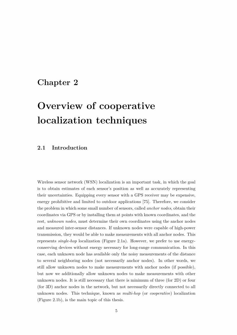
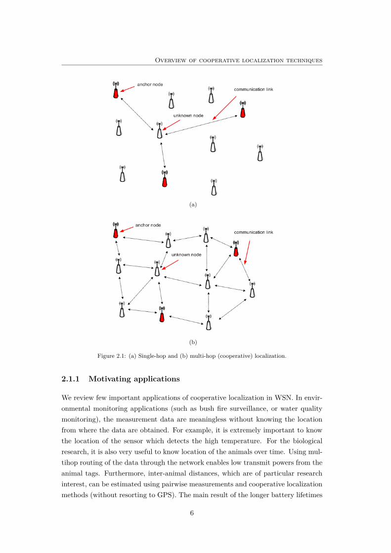
Wireless sensor network (WSN) localization is an important task, in which the goalis to obtain estimates of each sensor’s position as well as accurately representingtheir uncertainties. Equipping every sensor with a GPS receiver may be expensive,energy prohibitive and limited to outdoor applications [75]. Therefore, we considerthe problem in which some small number of sensors, called anchor nodes, obtain theircoordinates via GPS or by installing them at points with known coordinates, and therest, unknown nodes, must determine their own coordinates using the anchor nodesand measured inter-sensor distances. If unknown nodes were capable of high-powertransmission, they would be able to make measurements with all anchor nodes. Thisrepresents single-hop localization (Figure 2.1a). However, we prefer to use energy-conserving devices without energy necessary for long-range communication. In thiscase, each unknown node has available only the noisy measurements of the distanceto several neighboring nodes (not necessarily anchor nodes). In other words, westill allow unknown nodes to make measurements with anchor nodes (if possible),but now we additionally allow unknown nodes to make measurements with otherunknown nodes. It is still necessary that there is minimum of three (for 2D) or four(for 3D) anchor nodes in the network, but not necessarily directly connected to allunknown nodes. This technique, known as multi-hop (or cooperative) localization(Figure 2.1b), is the main topic of this thesis.
5
Overview of cooperative localization techniques
(a)
(b)
Figure 2.1: (a) Single-hop and (b) multi-hop (cooperative) localization.
2.1.1 Motivating applications
We review few important applications of cooperative localization in WSN. In envir-onmental monitoring applications (such as bush fire surveillance, or water qualitymonitoring), the measurement data are meaningless without knowing the locationfrom where the data are obtained. For example, it is extremely important to knowthe location of the sensor which detects the high temperature. For the biologicalresearch, it is also very useful to know location of the animals over time. Using mul-tihop routing of the data through the network enables low transmit powers from theanimal tags. Furthermore, inter-animal distances, which are of particular researchinterest, can be estimated using pairwise measurements and cooperative localizationmethods (without resorting to GPS). The main result of the longer battery lifetimes
6
2.1 Introduction
is less frequent recollaring of the animals. As another example, we can considerdeploying a sensor network in a manufacturing floor. The monitoring and control ofequipment has traditionally been wired, but making them wireless reduces the highcost of cabling and makes the manufacturing floor more dynamic. In addition, thesesensors monitor storage conditions (temperature and humidity) and help controlthe heating, ventilation, and air conditioning system. Sensors on mobile equipmentreport their location when the equipment is lost or needs to be found, and can evencontact security if the equipment is about to leave the building. Moreover, locationestimation may enable many of applications such as search-and-rescue, intrusion de-tection, road traffic monitoring, health monitoring, reconnaissance, and surveillance.A description of number of interesting applications can be found in [21,34,76,98].
2.1.2 Classification of cooperative localization methods
Range-based vs range-free methods
Range-free or connectivity-based localization methods [8, 68, 100, 101, 109] rely onconnectivity between the nodes. The principle of these algorithms is to determinewhether or not a sensor is in the transmission range of another sensor. The mostattractive feature of the range-free algorithms is their simplicity. However, theycan only provide a coarse grained estimate of each node’s location, which meansthat they are not only suitable for applications requiring precise location estimate.Range-based or distance-based localization algorithms [46,68,78,82,97] use the inter-sensor distance measurements in a sensor network to locate the entire network. Thistype of algorithms is usually more accurate, but sensitive to measurement errors.
Centralized vs distributed methods
Based on the approach of processing the individual inter-sensor data, localizationalgorithms can be also considered in two main classes: centralized and distributedalgorithms. Centralized algorithms [97, 100] utilize a single central processor (i.e.,fusion center) to collect all the individual inter-sensor data and produce a map of theentire sensor network, while distributed algorithms [46, 68, 82, 97, 118] rely on self-localization of each node in the sensor network using the local information it collectsfrom its neighbors. From the perspective of location estimation accuracy, centralizedalgorithms are likely to provide more accurate location estimates than distributedalgorithms. However, centralized algorithms suffer from the scalability problem,and generally are not feasible to be implemented for large scale WSN. On the otherhand, the main disadvantage of the distributed methods is that they require multiple
7
Overview of cooperative localization techniques
iterations to converge, which may cause the localization process to take long time.From the communication energy consumption perspective, centralized algorithmsin large-scale networks require each sensor’s measurements to be sent over multiplehops to the fusion center, while distributed algorithms require only local informationexchange between neighboring nodes but many such local exchanges may be required(depending on the number of iterations needed for convergence). If in a given sensornetwork and distributed algorithm, the average number of hops to the fusion centerexceeds the necessary number of iterations, then the distributed algorithm will bemore energy-efficient than a typical centralized algorithm [76].
Anchor-based vs anchor-free methods
Anchor-based [8, 68, 78, 97, 109] methods assume that a certain minimum numberof the nodes know their position, e.g., by manual placement or using some otherlocation mechanism such as GPS. This localization method has the limitation thatit needs another localization system to find the anchor node positions. In contrast,anchor-free [46,82,100,101] algorithms use local distance information to attempt todetermine node coordinates when no nodes have pre-defined positions. Of course,any such coordinate system will not be unique and can be embedded into anotherglobal coordinate space in infinitely many ways, depending on global translation,rotation, and flipping. Therefore, the main problem with anchor-free methods is theneed for an additional algorithm for transformation from the relative to the absolutecoordinates.
Probabilistic vs deterministic methods
Deterministic algorithms [68,82,97,100,101,109] use the measurements to estimatethe point estimate of the positions by applying classical least squares, multidimen-sional scaling, multilateration, or other optimization methods. In favor of theirrelative computational simplicity, they often lack a statistical interpretation, andas one consequence typically do not provide an estimate of the remaining uncer-tainty in each sensor location. However, iterative least-squares methods, like N -hop multilateration [97], have a straightforward statistical interpretation, by assum-ing a Gaussian model for all uncertainties, which may be questionable in practice.Non-Gaussian uncertainty is a common occurrence in real-world sensor localizationproblems, where there is usually some fraction of highly erroneous (outlier) meas-urements. On the other hand, probabilistic (or Bayesian) methods [8,46,48,78,118]take into account uncertainty of the measurements, so given the likelihood of e.g.,measured distance and a prior PDF of the positions of all unknown nodes, they
8
2.2 Measurement techniques
estimate the posterior PDF of the positions of all unknown nodes. However, themain drawback of the probabilistic methods is the high computational and com-munication cost which, in some applications, makes these methods unacceptable inlow-power WSN. Nevertheless, the particle-based approximation via nonparametricrepresentation, and an appropriate factorization of the PDFs, make probabilisticmethods acceptable for inference in sensor networks. In addition, nonparametricrepresentation enables us to estimate any PDF that does not exist in analytical(parametric) form.
2.2 Measurement techniques
Measurement techniques for WSN localization can be broadly classified into threecategories:
• Distance-based measurements (RSS, TOA, and TDOA)
• Angle-of-arrival (AOA) techniques
• RSS profiling techniques (fingerprinting)
We describe all of them in this section, with emphasis on the most commonused, distance related techniques. The detailed description can also be found in[43,63,76,98].
2.2.1 Received signal strength (RSS)
The goal of this technique is to estimate distance between neighboring sensors fromthe RSS measurements. These techniques are based on a standard feature foundin most wireless devices, a RSS indicator. They are attractive because they re-quire no additional hardware, and are unlikely to significantly impact local powerconsumption, sensor size and thus cost.
Let us denote this received power by Pr(d). This power varies as the inversesquare of the distance d between transmitter and receiver through the Friis equation:[84]:
Pr(d) = PtGtGrλ2
(4π)2d2 (2.1)
where Pt is the transmitted power, Gt is the transmitter antenna gain, Gr is thereceiver antenna gain, and λ is the wavelength of the transmitted signal in meters.However, the free-space model is an over-idealization, and the propagation of asignal is affected by reflection, diffraction and scattering. Of course, these effects are
9
Overview of cooperative localization techniques
environment (indoors, outdoors, rain, buildings, etc.) dependent. It is accepted onthe basis of empirical evidence to model RSS (Pr(d)) as a random and log-normallydistributed random variable with a distance dependent mean value:
Pr(d)[dBm] = P0(d0)[dBm]− 10np log10( dd0
) +Xσ (2.2)
where P0(d0) is known reference power value in dB milliwatts at a reference distancefrom the transmitter, np is the path loss exponent that measures the rate at whichthe RSS decreases with distance, typically between two and four depending on thespecific propagation environment, Xσ is a zero mean Gaussian distributed randomvariable with standard deviation σ and it accounts for the random effects of shad-owing. It is trivial to conclude from (2.2) that, given Pr(d)[dBm], the estimateddistance between a transmitter and receiver is:
d = d0 · 10−Pr(d)[dBm]−P0(d0)[dBm]
10np · 10Xσ
10np (2.3)
As we can see, the distance error is multiplicative (i.e., log-normally distributed)which means that RSS-based distance estimates have variance proportional to theirtrue distance. Therefore, RSS is most valuable in high-density sensor networks.
However, in addition to the path loss, measured RSS is also a function of thecalibration of both the transmitter and receiver. Depending on the expense of themanufacturing process, RSS indicator circuits and transmit powers will vary fromdevice to device. Also, transmit powers can change as batteries deplete. All theseproblems make RSS-based methods suitable only for coarse-grained localization.
2.2.2 Time of arrival (TOA)
Distances between neighboring sensors can be estimated from the propagation timemeasurements between transmitter and receiver, using two types of measurements,one-way and round-trip.
One-way propagation time measurements measure the difference between thesending time of a signal at the transmitter and the receiving time of the signal atthe receiver. It requires the local time at the transmitter and the local time atthe receiver to be accurately synchronized. This requirement may add to the costof sensors by demanding a highly accurate clock and/or increase the complexityof the sensor network by demanding a sophisticated synchronization mechanism.This disadvantage makes one-way propagation TOA measurements a less attractiveoption than measuring round-trip time in WSNs.
Round-trip propagation TOA measurements measure the difference between the
10
2.2 Measurement techniques
time when a signal is sent by a sensor and the time when the signal returned bya second sensor is received at the original sensor. Since the same clock is used tocompute the round-trip propagation time, there is no synchronization problem. Themajor error source in round-trip propagation TOA measurements is the delay re-quired for handling the signal in the second sensor. This internal delay is eitherknown via a priori calibration, or measured and sent to the first sensor to be sub-tracted.
A recent trend in propagation time measurements is the use of ultra-wide band(UWB) signals for accurate distance estimation [40, 102]. UWB is a signal whosefractional bandwidth (the ratio of its bandwidth to its center frequency) is largerthan 0.2 or a signal with a total bandwidth of more than 500 MHz. UWB canachieve higher accuracy because its bandwidth is very large and therefore its pulsehas a very short duration. This feature makes possible fine time resolution of UWBsignals and easy separation of multipath signals.
Generally, errors in TOA estimation are caused by two problems:
• Early-arriving multipath: Many multipath signals arrive very soon after theline-of-sight (LOS) signal, and their contributions to the cross-correlation ob-scure the location of the peak from the LOS signal.
• Attenuated LOS : The LOS signal can be severely attenuated compared to thelate-arriving multipath components, causing it to be “lost in the noise” andmissed completely; this leads to large positive errors in the TOA estimate.
2.2.3 Time difference of arrival (TDOA)
Taking time differences of TOA measurements eliminates the clock bias nuisanceparameter. This measurement is done between one transmitter and a number ofreceivers. The TDOA between a pair of receivers i and j is given by:
∆tij = ti − tj = 1c
(‖ri − rt‖ − ‖rj − rt‖) (2.4)
where ti and tj are the time when a signal is received at receivers, ri, rj and rt
is locations of transmitter, c is the propagation speed of the signal. However, themost widely used method is the generalized cross-correlation method [54], where thecross-correlation function between two signals si and si received at the receivers isgiven by:
ρij(τ) = 1T
T
0
si(t)sj(t− τ)dt (2.5)
11
Overview of cooperative localization techniques
The cross-correlation function can also be obtained from an inverse Fourier trans-form of the estimated frequency domain cross-spectral density function. Frequencydomain processing is often preferred because the signals can be filtered prior to com-putation of the cross-correlation function. The cross-correlation approach requiresvery accurate synchronization among receivers but does not impose any requirementon the signal transmitted by the transmitter.
This measurement technique is able to achieve better accuracy than RSS andTOA. However, the accuracy is achieved at the expense of higher equipment cost.The accuracy of TDOA measurements will improve when the separation betweenreceivers increases because this increases differences between time-of-arrival. Closelyspaced multiple receivers may give rise to multiple received signals that cannotbe separated. Another factor affecting the accuracy of TDOA measurements ismultipath. Overlapping cross-correlation peaks due to multipath usually cannot beresolved.
2.2.4 Lighthouse approach
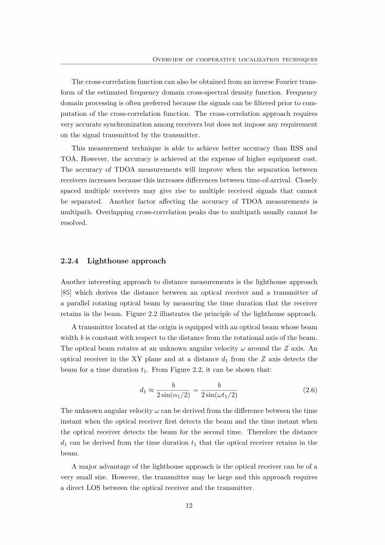
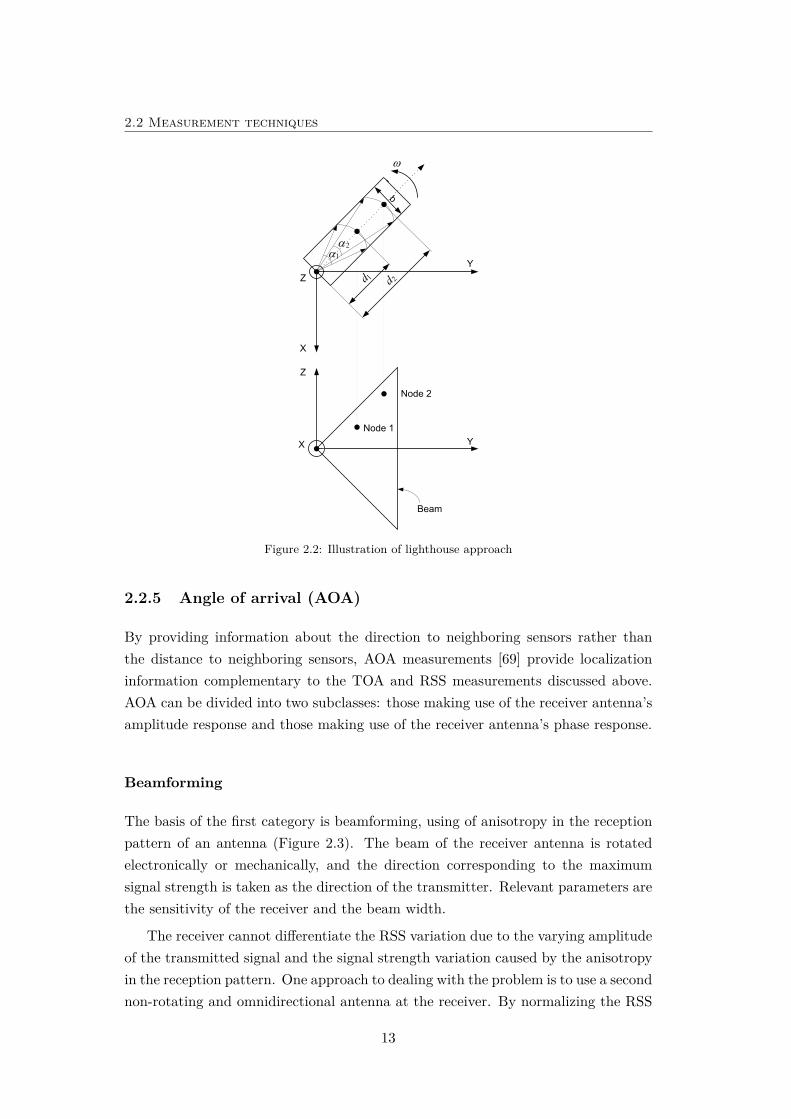
Another interesting approach to distance measurements is the lighthouse approach[85] which derives the distance between an optical receiver and a transmitter ofa parallel rotating optical beam by measuring the time duration that the receiverretains in the beam. Figure 2.2 illustrates the principle of the lighthouse approach.
A transmitter located at the origin is equipped with an optical beam whose beamwidth b is constant with respect to the distance from the rotational axis of the beam.The optical beam rotates at an unknown angular velocity ω around the Z axis. Anoptical receiver in the XY plane and at a distance d1 from the Z axis detects thebeam for a time duration t1. From Figure 2.2, it can be shown that:
d1 ≈b
2 sin(α1/2) = b
2 sin(ωt1/2) (2.6)
The unknown angular velocity ω can be derived from the difference between the timeinstant when the optical receiver first detects the beam and the time instant whenthe optical receiver detects the beam for the second time. Therefore the distanced1 can be derived from the time duration t1 that the optical receiver retains in thebeam.
A major advantage of the lighthouse approach is the optical receiver can be of avery small size. However, the transmitter may be large and this approach requiresa direct LOS between the optical receiver and the transmitter.
12
2.2 Measurement techniques
ω
1d 2d
1α2α
Figure 2.2: Illustration of lighthouse approach
2.2.5 Angle of arrival (AOA)
By providing information about the direction to neighboring sensors rather thanthe distance to neighboring sensors, AOA measurements [69] provide localizationinformation complementary to the TOA and RSS measurements discussed above.AOA can be divided into two subclasses: those making use of the receiver antenna’samplitude response and those making use of the receiver antenna’s phase response.
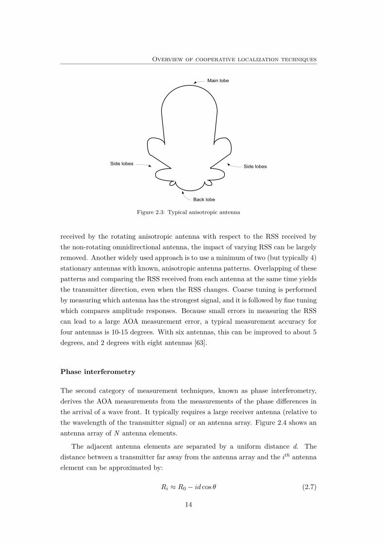
Beamforming
The basis of the first category is beamforming, using of anisotropy in the receptionpattern of an antenna (Figure 2.3). The beam of the receiver antenna is rotatedelectronically or mechanically, and the direction corresponding to the maximumsignal strength is taken as the direction of the transmitter. Relevant parameters arethe sensitivity of the receiver and the beam width.
The receiver cannot differentiate the RSS variation due to the varying amplitudeof the transmitted signal and the signal strength variation caused by the anisotropyin the reception pattern. One approach to dealing with the problem is to use a secondnon-rotating and omnidirectional antenna at the receiver. By normalizing the RSS
13
Overview of cooperative localization techniques
Figure 2.3: Typical anisotropic antenna
received by the rotating anisotropic antenna with respect to the RSS received bythe non-rotating omnidirectional antenna, the impact of varying RSS can be largelyremoved. Another widely used approach is to use a minimum of two (but typically 4)stationary antennas with known, anisotropic antenna patterns. Overlapping of thesepatterns and comparing the RSS received from each antenna at the same time yieldsthe transmitter direction, even when the RSS changes. Coarse tuning is performedby measuring which antenna has the strongest signal, and it is followed by fine tuningwhich compares amplitude responses. Because small errors in measuring the RSScan lead to a large AOA measurement error, a typical measurement accuracy forfour antennas is 10-15 degrees. With six antennas, this can be improved to about 5degrees, and 2 degrees with eight antennas [63].
Phase interferometry
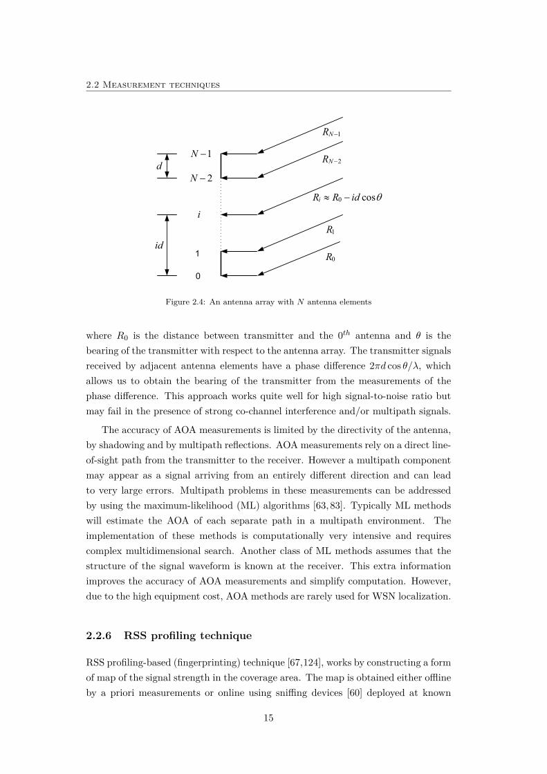
The second category of measurement techniques, known as phase interferometry,derives the AOA measurements from the measurements of the phase differences inthe arrival of a wave front. It typically requires a large receiver antenna (relative tothe wavelength of the transmitter signal) or an antenna array. Figure 2.4 shows anantenna array of N antenna elements.
The adjacent antenna elements are separated by a uniform distance d. Thedistance between a transmitter far away from the antenna array and the ith antennaelement can be approximated by:
Ri ≈ R0 − id cos θ (2.7)
14
2.2 Measurement techniques
0 cosiR R id θ≈ −
0R
1R
2NR −
1NR −
i
1N −
2N −
id
d
Figure 2.4: An antenna array with N antenna elements
where R0 is the distance between transmitter and the 0th antenna and θ is thebearing of the transmitter with respect to the antenna array. The transmitter signalsreceived by adjacent antenna elements have a phase difference 2πd cos θ/λ, whichallows us to obtain the bearing of the transmitter from the measurements of thephase difference. This approach works quite well for high signal-to-noise ratio butmay fail in the presence of strong co-channel interference and/or multipath signals.
The accuracy of AOA measurements is limited by the directivity of the antenna,by shadowing and by multipath reflections. AOA measurements rely on a direct line-of-sight path from the transmitter to the receiver. However a multipath componentmay appear as a signal arriving from an entirely different direction and can leadto very large errors. Multipath problems in these measurements can be addressedby using the maximum-likelihood (ML) algorithms [63, 83]. Typically ML methodswill estimate the AOA of each separate path in a multipath environment. Theimplementation of these methods is computationally very intensive and requirescomplex multidimensional search. Another class of ML methods assumes that thestructure of the signal waveform is known at the receiver. This extra informationimproves the accuracy of AOA measurements and simplify computation. However,due to the high equipment cost, AOA methods are rarely used for WSN localization.
2.2.6 RSS profiling technique
RSS profiling-based (fingerprinting) technique [67,124], works by constructing a formof map of the signal strength in the coverage area. The map is obtained either offlineby a priori measurements or online using sniffing devices [60] deployed at known
15
Overview of cooperative localization techniques
locations. They have been mainly used for location estimation in wireless local areanetworks (WLAN), but they would appear to be attractive also for WSN. In thistechnique, in addition to anchor nodes (e.g. access points in WLANs) and non-anchor nodes, a large number of sample points (e.g. sniffing devices) are distributedthroughout the coverage area of the WSN. At each sample point, a vector of RSSis obtained, with the ith entry corresponding to the ith anchor’s transmitted signal.Of course, many entries of the signal strength vector may be zero or very small,corresponding to anchor nodes at larger distances (relative to the transmission rangeor sensing radius) from the sample point. The collection of all these vectors provides(by extrapolation in the vicinity of the sample points) a map of the whole region.The collection constitutes the RSS model, and it is unique with respect to theanchor locations and the environment. The model is stored in a central location.By referring to the RSS model, a non-anchor node can estimate its location using theRSS measurements from anchors. However, the main problem of this approach issensitivity to environmental changes. In that case, the system must be re-calibrated,i.e., new vector of RSS have to be collected.
2.3 Deterministic localization techniques
In this section, we review deterministic (or non-Bayesian) localization techniques,in which the main goal is to find the point estimate of the sensor positions. Inparticular, we focus on connectivity-based and distance-based cooperative localiza-tion algorithms due to their prevalence in cooperative WSN localization. For bothclasses, we describe few centralized and distributed algorithms. In addition, wedescribe a method for localization using AOA measurements.
2.3.1 Connectivity based algorithms
Connectivity-based or “range-free” localization algorithms do not rely on any of themeasurement techniques described in Section 2.2. Instead they use the connectiv-ity information to estimate the location of the unknown nodes (i.e., who is withinthe communication range). We will describe three algorithms in subsequent sec-tions: distributed ad-hoc positioning based on the distance-vector-hop (DV-hop)approach [68], centralized and distributed algorithm based on multi-dimensionalscaling (MDS) [100,101], and distributed concentric anchor beacon (CAB) [109].
16
2.3 Deterministic localization techniques
Ad-hoc positioning
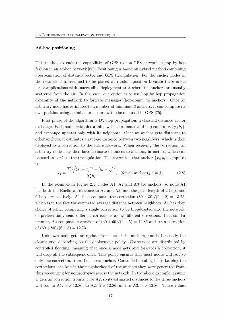
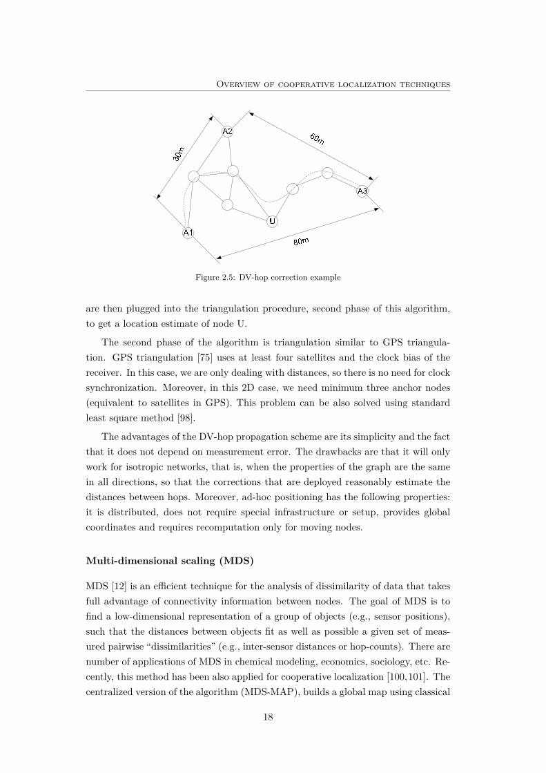
This method extends the capabilities of GPS to non-GPS network in hop by hopfashion in an ad-hoc network [68]. Positioning is based on hybrid method combiningapproximation of distance vector and GPS triangulation. For the anchor nodes inthe network it is assumed to be placed at random position because there are alot of applications with inaccessible deployment area where the anchors are usuallyscattered from the air. In this case, one option is to use hop by hop propagationcapability of the network to forward messages (hop-count) to anchors. Once anarbitrary node has estimates to a number of minimum 3 anchors, it can compute itsown position using a similar procedure with the one used in GPS [75].
First phase of the algorithm is DV-hop propagation, a classical distance vectorexchange. Each node maintains a table with coordinates and hop-counts {xi, yi, hi},and exchange updates only with its neighbors. Once an anchor gets distances toother anchors, it estimates a average distance between two neighbors, which is thendeployed as a correction to the entire network. When receiving the correction, anarbitrary node may then have estimate distances to anchors, in meters, which canbe used to perform the triangulation. The correction that anchor {xi, yi} computesis:
ci =∑√
(xi − xj)2 + (yi − yj)2∑hi
, (for all anchors j, i 6= j) (2.8)
In the example in Figure 2.5, nodes A1, A2 and A3 are anchors, so node A1has both the Euclidean distance to A2 and A3, and the path length of 2 hops and6 hops, respectively. A1 then computes the correction (80 + 30)/(6 + 2) = 13.75,which is in the fact the estimated average distance between neighbors. A1 has thenchoice of either computing a single correction to be broadcasted into the network,or preferentially send different corrections along different directions. In a similarmanner, A2 computes correction of (30 + 60)/(2 + 5) = 12.86 and A3 a correctionof (60 + 80)/(6 + 5) = 12.73.
Unknown node gets an update from one of the anchors, and it is usually theclosest one, depending on the deployment policy. Corrections are distributed bycontrolled flooding, meaning that once a node gets and forwards a correction, itwill drop all the subsequent ones. This policy ensures that most nodes will receiveonly one correction, from the closest anchor. Controlled flooding helps keeping thecorrections localized in the neighborhood of the anchors they were generated from,thus accounting for nonisotropies across the network. In the above example, assumeU gets an correction from anchor A2, so its estimated distances to the three anchorswill be: to A1: 3 × 12.86, to A2: 2 × 12.86, and to A3: 3 × 12.86. These values
17
Overview of cooperative localization techniques
Figure 2.5: DV-hop correction example
are then plugged into the triangulation procedure, second phase of this algorithm,to get a location estimate of node U.
The second phase of the algorithm is triangulation similar to GPS triangula-tion. GPS triangulation [75] uses at least four satellites and the clock bias of thereceiver. In this case, we are only dealing with distances, so there is no need for clocksynchronization. Moreover, in this 2D case, we need minimum three anchor nodes(equivalent to satellites in GPS). This problem can be also solved using standardleast square method [98].
The advantages of the DV-hop propagation scheme are its simplicity and the factthat it does not depend on measurement error. The drawbacks are that it will onlywork for isotropic networks, that is, when the properties of the graph are the samein all directions, so that the corrections that are deployed reasonably estimate thedistances between hops. Moreover, ad-hoc positioning has the following properties:it is distributed, does not require special infrastructure or setup, provides globalcoordinates and requires recomputation only for moving nodes.
Multi-dimensional scaling (MDS)
MDS [12] is an efficient technique for the analysis of dissimilarity of data that takesfull advantage of connectivity information between nodes. The goal of MDS is tofind a low-dimensional representation of a group of objects (e.g., sensor positions),such that the distances between objects fit as well as possible a given set of meas-ured pairwise “dissimilarities” (e.g., inter-sensor distances or hop-counts). There arenumber of applications of MDS in chemical modeling, economics, sociology, etc. Re-cently, this method has been also applied for cooperative localization [100,101]. Thecentralized version of the algorithm (MDS-MAP), builds a global map using classical
18
2.3 Deterministic localization techniques
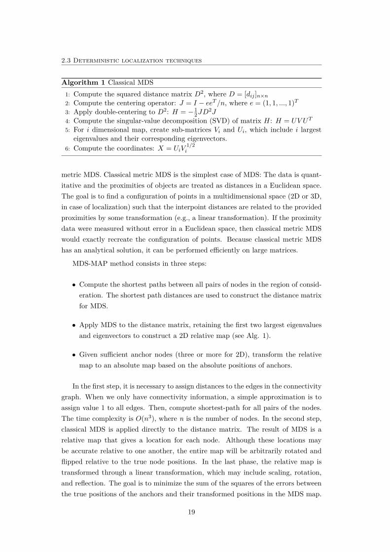
Algorithm 1 Classical MDS1: Compute the squared distance matrix D2, where D = [dij ]n×n2: Compute the centering operator: J = I − eeT /n, where e = (1, 1, ..., 1)T3: Apply double-centering to D2: H = −1
2JD2J
4: Compute the singular-value decomposition (SVD) of matrix H: H = UV UT
5: For i dimensional map, create sub-matrices Vi and Ui, which include i largesteigenvalues and their corresponding eigenvectors.
6: Compute the coordinates: X = UiV1/2i
metric MDS. Classical metric MDS is the simplest case of MDS: The data is quant-itative and the proximities of objects are treated as distances in a Euclidean space.The goal is to find a configuration of points in a multidimensional space (2D or 3D,in case of localization) such that the interpoint distances are related to the providedproximities by some transformation (e.g., a linear transformation). If the proximitydata were measured without error in a Euclidean space, then classical metric MDSwould exactly recreate the configuration of points. Because classical metric MDShas an analytical solution, it can be performed efficiently on large matrices.
MDS-MAP method consists in three steps:
• Compute the shortest paths between all pairs of nodes in the region of consid-eration. The shortest path distances are used to construct the distance matrixfor MDS.
• Apply MDS to the distance matrix, retaining the first two largest eigenvaluesand eigenvectors to construct a 2D relative map (see Alg. 1).
• Given sufficient anchor nodes (three or more for 2D), transform the relativemap to an absolute map based on the absolute positions of anchors.
In the first step, it is necessary to assign distances to the edges in the connectivitygraph. When we only have connectivity information, a simple approximation is toassign value 1 to all edges. Then, compute shortest-path for all pairs of the nodes.The time complexity is O(n3), where n is the number of nodes. In the second step,classical MDS is applied directly to the distance matrix. The result of MDS is arelative map that gives a location for each node. Although these locations maybe accurate relative to one another, the entire map will be arbitrarily rotated andflipped relative to the true node positions. In the last phase, the relative map istransformed through a linear transformation, which may include scaling, rotation,and reflection. The goal is to minimize the sum of the squares of the errors betweenthe true positions of the anchors and their transformed positions in the MDS map.
19
Overview of cooperative localization techniques
Computing the transformation parameters takes O(m3) time, wherem is the numberof anchors.
MDP-MAP does not work well on irregular networks, because it relies on shortest-path distance estimation, which can have large errors for remote nodes. Anotherproblem with this centralized method is that it is not applied easily to large net-works for which reading out the connectivity and distance information is potentiallyprohibitive. The improved version of MDS-MAP, called MDS-MAP-P, addressesboth of these problems.
MDS-MAP-P builds many local maps and then patches them together to form aglobal map. This method relies on local information and avoids using the distanceestimation between remote notes, so it achieves better results on irregular networks.Individual nodes simultaneously compute their own local maps using their local in-formation. Then, these maps can be incrementally merged to form a global map.Therefore, another benefit is that this algorithm can be easily executed in a distrib-uted fashion. MDS-MAP-P method consists in four steps:
• Set the range for local maps, Rlm. For each node, neighbors within Rlm hopsare involved in building its local map.
• For each node, apply MDS-MAP to the nodes within range Rlm to generateits local map.
• Merge local maps [100,101].
• Given sufficient anchor nodes (three or more for 2D), transform the relativemap to an absolute map based on the absolute positions of anchors.
The strength of both approaches is that it can be used when there are few orno anchor nodes. This approach also does not have limitation about anchor nodeplacement. It builds a relative map of the nodes even when no anchor nodes areavailable. With three or more anchor nodes, the relative map can be transformedinto absolute coordinates. An optional refinement step can be used to further im-prove the quality of the solution, at the expense of additional computation. Thisvariant of MDS-MAP (MDS-MAP-PR) [101] requires measured distances betweenthe neighboring nodes (see Section 2.3.2). A patching-based variation not only al-lows distributed and parallel computation, but also gives better solutions, especiallyon irregularly-shaped networks.
20
2.3 Deterministic localization techniques
1r
maxrmaxr
1r
2r2r
Figure 2.6: Anchor beacon transmission ranges for (a) CAB-EA, and (b) CAB-EW
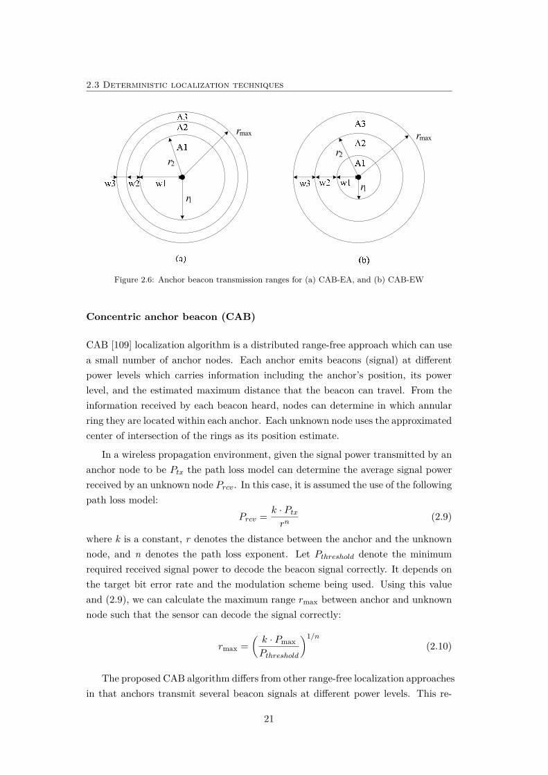
Concentric anchor beacon (CAB)
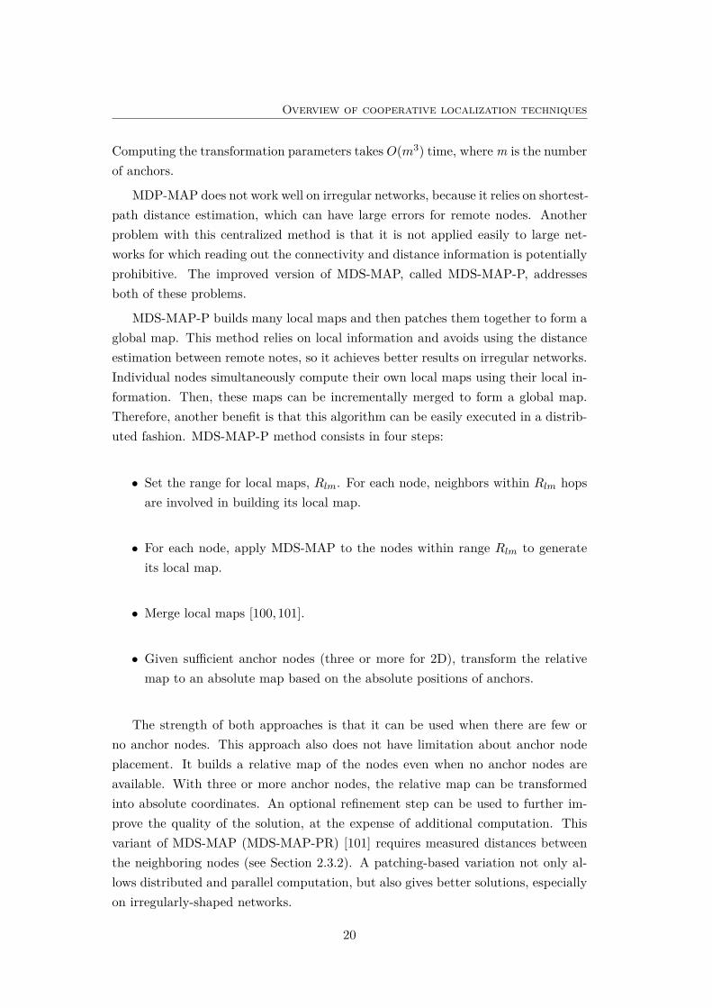
CAB [109] localization algorithm is a distributed range-free approach which can usea small number of anchor nodes. Each anchor emits beacons (signal) at differentpower levels which carries information including the anchor’s position, its powerlevel, and the estimated maximum distance that the beacon can travel. From theinformation received by each beacon heard, nodes can determine in which annularring they are located within each anchor. Each unknown node uses the approximatedcenter of intersection of the rings as its position estimate.
In a wireless propagation environment, given the signal power transmitted by ananchor node to be Ptx the path loss model can determine the average signal powerreceived by an unknown node Prcv. In this case, it is assumed the use of the followingpath loss model:
Prcv = k · Ptxrn
(2.9)
where k is a constant, r denotes the distance between the anchor and the unknownnode, and n denotes the path loss exponent. Let Pthreshold denote the minimumrequired received signal power to decode the beacon signal correctly. It depends onthe target bit error rate and the modulation scheme being used. Using this valueand (2.9), we can calculate the maximum range rmax between anchor and unknownnode such that the sensor can decode the signal correctly:
rmax =(k · PmaxPthreshold
)1/n(2.10)
The proposed CAB algorithm differs from other range-free localization approachesin that anchors transmit several beacon signals at different power levels. This re-
21
Overview of cooperative localization techniques
quirement is feasible in current WSNs. Ideally, the different power levels dividethe possible transmission ranges of an anchor into a circle and rings. The lowestpower level creates a circular coverage area, and the following higher levels are dis-tinguished by rings emanating from this lowest level. There are two variations of thisalgorithm (Figure 2.6). In CAB-EA, it is assumed that the area of the innermostcircle and the rings are all the same; and in CAB-EW, it is assumed that the widthof the innermost circle and the rings are all the same.
The relationship between the ith transmitting beacon power level Pi and themaximum transmitting power level Pmax is calculated using (2.9) and the relation-ship between the beacon transmission ranges ri and the maximum transmissionrange rmax (according to Figure 2.6). For CAB-EA and CAB-EW, these powers arerespectively given by:
Pi =(i
m
)n2Pmax, Pi =
(i
m
)nPmax (2.11)
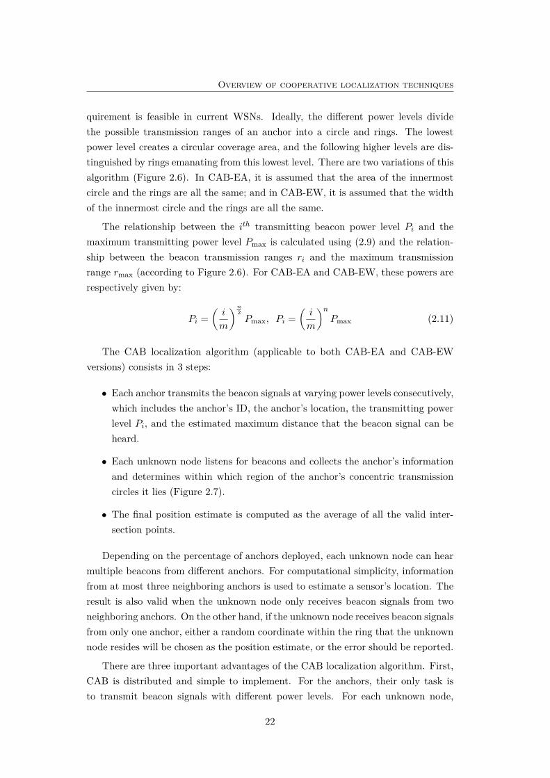
The CAB localization algorithm (applicable to both CAB-EA and CAB-EWversions) consists in 3 steps:
• Each anchor transmits the beacon signals at varying power levels consecutively,which includes the anchor’s ID, the anchor’s location, the transmitting powerlevel Pi, and the estimated maximum distance that the beacon signal can beheard.
• Each unknown node listens for beacons and collects the anchor’s informationand determines within which region of the anchor’s concentric transmissioncircles it lies (Figure 2.7).
• The final position estimate is computed as the average of all the valid inter-section points.
Depending on the percentage of anchors deployed, each unknown node can hearmultiple beacons from different anchors. For computational simplicity, informationfrom at most three neighboring anchors is used to estimate a sensor’s location. Theresult is also valid when the unknown node only receives beacon signals from twoneighboring anchors. On the other hand, if the unknown node receives beacon signalsfrom only one anchor, either a random coordinate within the ring that the unknownnode resides will be chosen as the position estimate, or the error should be reported.
There are three important advantages of the CAB localization algorithm. First,CAB is distributed and simple to implement. For the anchors, their only task isto transmit beacon signals with different power levels. For each unknown node,
22
2.3 Deterministic localization techniques
A
B
C
anchor
Valid intersection points
Node
Estimate
Figure 2.7: Example of localization using CAB
the determination of the intersection points from three chosen anchors as well asthe position estimate by averaging are not computationally intensive. Second, noinformation exchange between neighboring sensors is necessary. This reduces theenergy requirement for localization. And third, maintain high accuracy comparingto other connectivity-based algorithms. On the other hand, a sensor has to be ableto transmit several beacon signals at sufficient number of power levels, what makesthis method expensive.
2.3.2 Distance based algorithms
The core of distance based localization algorithms is the use of inter-sensor distancemeasurements in a WSN to locate the entire network. The main measurementstechniques used for this approach are described in Section 2.2.1. We first describethe extension of connectivity based algorithms (Section 2.3.1) to make them applic-able for distance based methods. Then, we will provide the detailed description oftwo well-known algorithms: collaborative (N-hop) multilateration (distributed andcentralized version) [97], and anchor-free distributed (AFL) localization [82].
Extension of connectivity-based algorithms
The centralized MDS-MAP approach [100,101], used in the connectivity-based local-ization algorithms described in Section 2.3.1, can be readily extended to incorporatedistance measurements into the corresponding optimization problem. Only a refine-ment step has to be added between steps 2 and 3. In this step, using the positionestimates of nodes in the MDS solution as an initial solution, least-squares min-imization can be applied to improve the match between the measured distances
23
Overview of cooperative localization techniques
between neighboring nodes and their distances in the solution. However, the mainproblem of this approach is that we cannot easily and accurately estimate n-hopdistances (n=2,3...). Alternative approach [50] tries to estimate these distances us-ing iterative MDS, in which random initial configuration of the nodes is used for thecomputation of unavailable distances. Another method, distributed weighted MDS(DW-MDS) [23], uses weights to quantify the accuracy of the measurements betweeneach pair of the nodes. Hence, if the measurement is not available, the weight is setto zero.
Distributed ad-hoc DV-hop algorithm, described in Section 2.3.1, can be exten-ded to incorporate distance measurements. A modified version of this algorithm,called DV-distance [68], includes distance measurements into the localization pro-cess. The only difference is propagation of measured distance among neighboringnodes instead of hop-count.
Collaborative (N-hop) multilateration
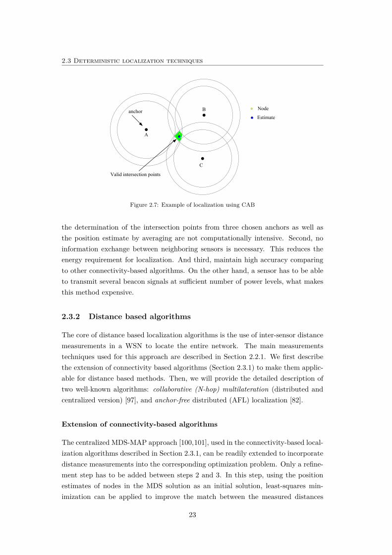
The collaborative multilateration [97] algorithm will be presented in two computa-tion models, centralized and distributed. In centralized algorithm all computationtakes place at a base station, and in distributed algorithm computation takes placeat every node. One of the main challenges in this algorithm is to prevent error accu-mulation inside the network. To prevent it, the node localization problem is set upas a least squares estimation problem with respect to the global network topology.Collaborative multilateration takes place in three main phases:
• Formation of collaborative subtrees
• Computation of initial estimates
• Position refinement
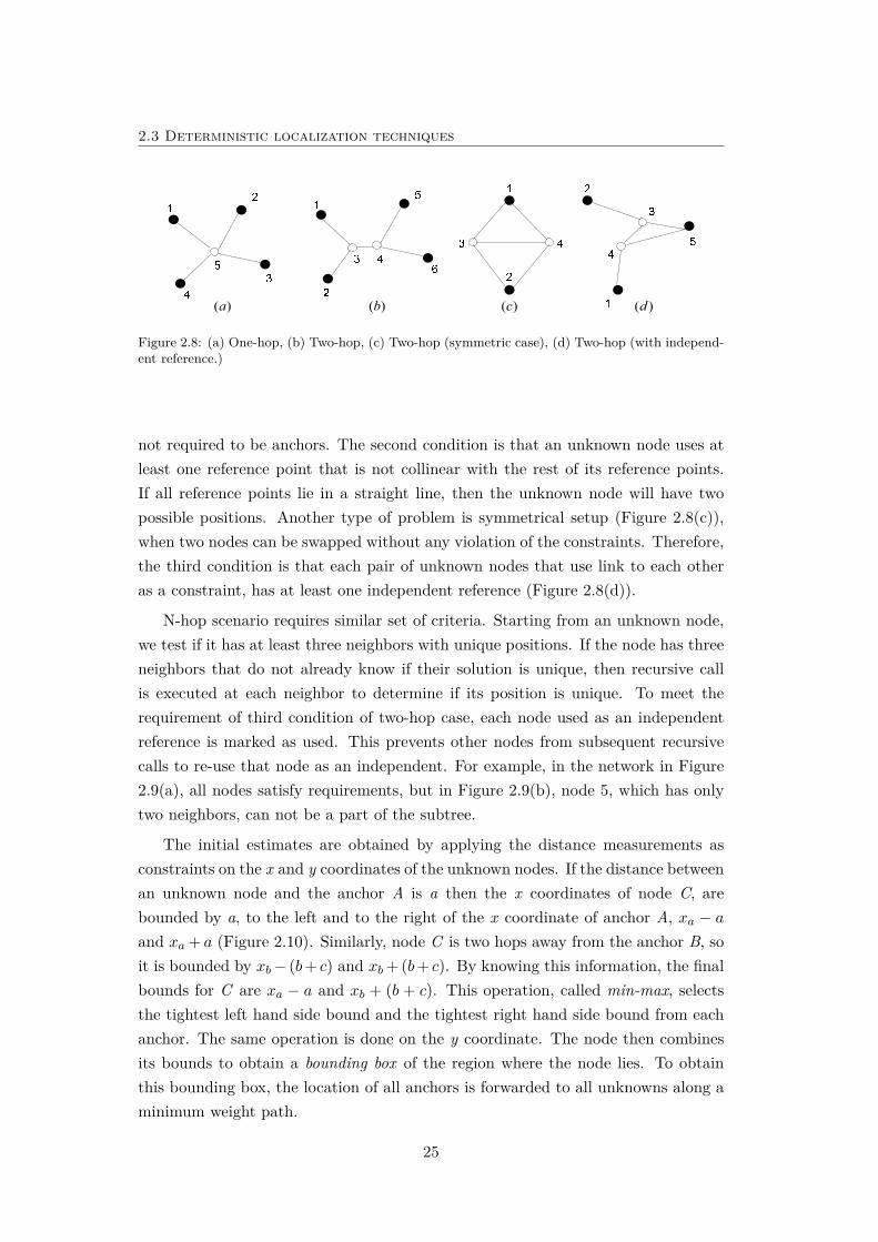
In the first phase, it is necessary to form the subtrees. Collaborative subtreesconstitutes a configuration of unknowns and anchors for which the estimated locationcan be uniquely determined. The nodes that do not meet the criteria for collabor-ative subtrees cannot participate in this configuration. The position estimates forsuch nodes are determined later in a post-processing phase. In the single-hop setupof Figure 2.8(a), the basic requirement for unknown node is that it is within range ofat least three anchors which are not lie in a straight line. A two-hop scenario (Figure2.8(b)) represents the case where the anchors are not always directly connected tothe node, but they are within a two-hop radius from the unknown node. In thiscase, the first condition is the same like for one-hop scenario, but these nodes are
24
2.3 Deterministic localization techniques
( )a ( )b ( )c ( )d
Figure 2.8: (a) One-hop, (b) Two-hop, (c) Two-hop (symmetric case), (d) Two-hop (with independ-ent reference.)
not required to be anchors. The second condition is that an unknown node uses atleast one reference point that is not collinear with the rest of its reference points.If all reference points lie in a straight line, then the unknown node will have twopossible positions. Another type of problem is symmetrical setup (Figure 2.8(c)),when two nodes can be swapped without any violation of the constraints. Therefore,the third condition is that each pair of unknown nodes that use link to each otheras a constraint, has at least one independent reference (Figure 2.8(d)).
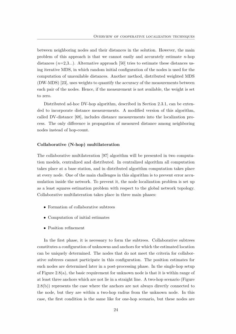
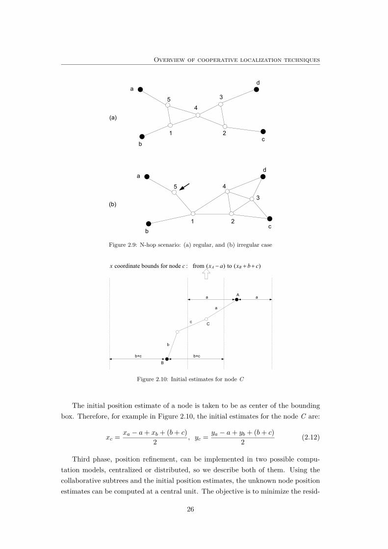
N-hop scenario requires similar set of criteria. Starting from an unknown node,we test if it has at least three neighbors with unique positions. If the node has threeneighbors that do not already know if their solution is unique, then recursive callis executed at each neighbor to determine if its position is unique. To meet therequirement of third condition of two-hop case, each node used as an independentreference is marked as used. This prevents other nodes from subsequent recursivecalls to re-use that node as an independent. For example, in the network in Figure2.9(a), all nodes satisfy requirements, but in Figure 2.9(b), node 5, which has onlytwo neighbors, can not be a part of the subtree.
The initial estimates are obtained by applying the distance measurements asconstraints on the x and y coordinates of the unknown nodes. If the distance betweenan unknown node and the anchor A is a then the x coordinates of node C, arebounded by a, to the left and to the right of the x coordinate of anchor A, xa − aand xa + a (Figure 2.10). Similarly, node C is two hops away from the anchor B, soit is bounded by xb− (b+ c) and xb + (b+ c). By knowing this information, the finalbounds for C are xa − a and xb + (b + c). This operation, called min-max, selectsthe tightest left hand side bound and the tightest right hand side bound from eachanchor. The same operation is done on the y coordinate. The node then combinesits bounds to obtain a bounding box of the region where the node lies. To obtainthis bounding box, the location of all anchors is forwarded to all unknowns along aminimum weight path.
25
Overview of cooperative localization techniques
5
1 2
3
4
a
bc
d
5
1 2
3
4
a
bc
d
(a)
(b)
Figure 2.9: N-hop scenario: (a) regular, and (b) irregular case
a
b
c
A
B
C
a a
b+cb+c
coordinate bounds for node : from ( ) to ( )A Bx c x a x b c− + +
Figure 2.10: Initial estimates for node C
The initial position estimate of a node is taken to be as center of the boundingbox. Therefore, for example in Figure 2.10, the initial estimates for the node C are:
xc = xa − a+ xb + (b+ c)2 , yc = ya − a+ yb + (b+ c)
2 (2.12)
Third phase, position refinement, can be implemented in two possible compu-tation models, centralized or distributed, so we describe both of them. Using thecollaborative subtrees and the initial position estimates, the unknown node positionestimates can be computed at a central unit. The objective is to minimize the resid-
26
2.3 Deterministic localization techniques
uals between the measured distances between the nodes and the distances computedin second phase using equation:
fij = dij −√
(exi − xj)2 + (eyi − yj)2 (2.13)
where dij represents the measured distance between nodes i and j, fij is residualbetween measured and estimated quantities, and the prefix e in front of x and ydenotes estimated coordinates as opposed to known coordinates. The objective isto minimize the mean square error over all equations:
F (xi, yi, xi+1, yi+1, ...) = min∑
f2ij (2.14)
The solution to this optimization problem can be obtained using some of the stand-ard least squares methods, for example Kalman filter (KF) [116]. A KF consists oftwo phases, a time update phase and a measurement update phase. For this pur-pose, the network is assumed to be static, the positions of the nodes do not changein time, so the time update phase is not used. The measurement update phase isgiven by the next set of equations:
Kk = P−k HT(HP−k H
T +R)−1
(2.15)
xk = Kk (zk − zk) + x−k (2.16)
Pk = (I −KkH)P−k (2.17)
where vector x−k represents initial estimates, xk represents new estimates after themeasurements update phases, P−k is the a priori estimate of the error covariance,Pk is the new estimate after the measurement update phase. Kk represents the KFgain and it serves a weight to the residual of the filter. The residual is the differencebetween the measurements (represented by zk) and the predicted measurement (zk =Hx−k ). Vector zk is the distance between the nodes, based on the current positionestimate, so matrix H is the Jacobian of zk with respect to the a priori estimates(x−k ) of the location. Matrix R is the measurement noise covariance matrix, whichcontains the known covariance of the distance measurement system (e.g., Gaussiannoise). Alg. 2 shows how to estimate the unknown locations.
Each edge in the collaborative subtree contributes one entry in the measurementmatrix zk. In matrix H, the number of unknown nodes determines the number ofcolumns and the number of edges determines the number of rows. The noise cov-ariance matrices (Pk, P−k ) are square matrices whose size depends on the numberof unknown nodes (a priori value P−k is set to the identity matrix). The measure-ment noise matrix R is a square matrix with size determined by number of edges in
27
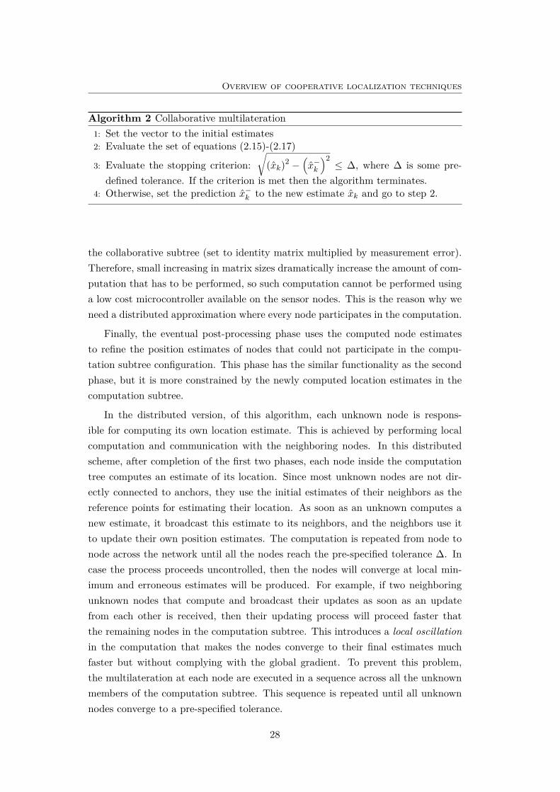
Overview of cooperative localization techniques
Algorithm 2 Collaborative multilateration1: Set the vector to the initial estimates2: Evaluate the set of equations (2.15)-(2.17)
3: Evaluate the stopping criterion:√
(xk)2 −(x−k
)2≤ ∆, where ∆ is some pre-
defined tolerance. If the criterion is met then the algorithm terminates.4: Otherwise, set the prediction x−k to the new estimate xk and go to step 2.
the collaborative subtree (set to identity matrix multiplied by measurement error).Therefore, small increasing in matrix sizes dramatically increase the amount of com-putation that has to be performed, so such computation cannot be performed usinga low cost microcontroller available on the sensor nodes. This is the reason why weneed a distributed approximation where every node participates in the computation.
Finally, the eventual post-processing phase uses the computed node estimatesto refine the position estimates of nodes that could not participate in the compu-tation subtree configuration. This phase has the similar functionality as the secondphase, but it is more constrained by the newly computed location estimates in thecomputation subtree.
In the distributed version, of this algorithm, each unknown node is respons-ible for computing its own location estimate. This is achieved by performing localcomputation and communication with the neighboring nodes. In this distributedscheme, after completion of the first two phases, each node inside the computationtree computes an estimate of its location. Since most unknown nodes are not dir-ectly connected to anchors, they use the initial estimates of their neighbors as thereference points for estimating their location. As soon as an unknown computes anew estimate, it broadcast this estimate to its neighbors, and the neighbors use itto update their own position estimates. The computation is repeated from node tonode across the network until all the nodes reach the pre-specified tolerance ∆. Incase the process proceeds uncontrolled, then the nodes will converge at local min-imum and erroneous estimates will be produced. For example, if two neighboringunknown nodes that compute and broadcast their updates as soon as an updatefrom each other is received, then their updating process will proceed faster thatthe remaining nodes in the computation subtree. This introduces a local oscillationin the computation that makes the nodes converge to their final estimates muchfaster but without complying with the global gradient. To prevent this problem,the multilateration at each node are executed in a sequence across all the unknownmembers of the computation subtree. This sequence is repeated until all unknownnodes converge to a pre-specified tolerance.
28
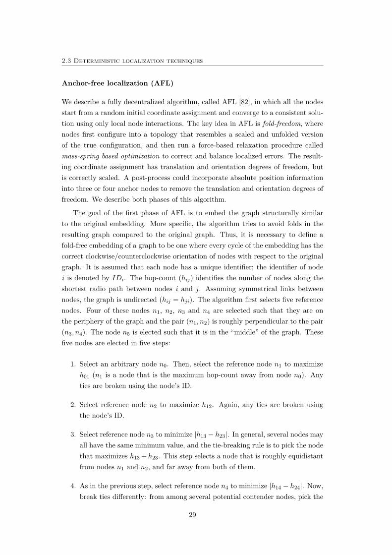
2.3 Deterministic localization techniques
Anchor-free localization (AFL)
We describe a fully decentralized algorithm, called AFL [82], in which all the nodesstart from a random initial coordinate assignment and converge to a consistent solu-tion using only local node interactions. The key idea in AFL is fold-freedom, wherenodes first configure into a topology that resembles a scaled and unfolded versionof the true configuration, and then run a force-based relaxation procedure calledmass-spring based optimization to correct and balance localized errors. The result-ing coordinate assignment has translation and orientation degrees of freedom, butis correctly scaled. A post-process could incorporate absolute position informationinto three or four anchor nodes to remove the translation and orientation degrees offreedom. We describe both phases of this algorithm.
The goal of the first phase of AFL is to embed the graph structurally similarto the original embedding. More specific, the algorithm tries to avoid folds in theresulting graph compared to the original graph. Thus, it is necessary to define afold-free embedding of a graph to be one where every cycle of the embedding has thecorrect clockwise/counterclockwise orientation of nodes with respect to the originalgraph. It is assumed that each node has a unique identifier; the identifier of nodei is denoted by IDi. The hop-count (hij) identifies the number of nodes along theshortest radio path between nodes i and j. Assuming symmetrical links betweennodes, the graph is undirected (hij = hji). The algorithm first selects five referencenodes. Four of these nodes n1, n2, n3 and n4 are selected such that they are onthe periphery of the graph and the pair (n1, n2) is roughly perpendicular to the pair(n3, n4). The node n5 is elected such that it is in the “middle” of the graph. Thesefive nodes are elected in five steps:
1. Select an arbitrary node n0. Then, select the reference node n1 to maximizeh01 (n1 is a node that is the maximum hop-count away from node n0). Anyties are broken using the node’s ID.
2. Select reference node n2 to maximize h12. Again, any ties are broken usingthe node’s ID.
3. Select reference node n3 to minimize |h13 − h23|. In general, several nodes mayall have the same minimum value, and the tie-breaking rule is to pick the nodethat maximizes h13 + h23. This step selects a node that is roughly equidistantfrom nodes n1 and n2, and far away from both of them.
4. As in the previous step, select reference node n4 to minimize |h14 − h24|. Now,break ties differently: from among several potential contender nodes, pick the
29
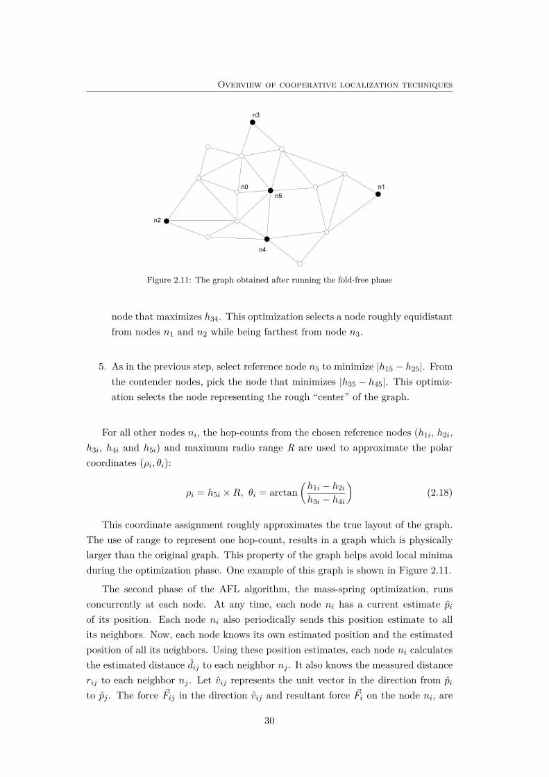
Overview of cooperative localization techniques
n0 n1
n2
n3
n4
n5
Figure 2.11: The graph obtained after running the fold-free phase
node that maximizes h34. This optimization selects a node roughly equidistantfrom nodes n1 and n2 while being farthest from node n3.
5. As in the previous step, select reference node n5 to minimize |h15 − h25|. Fromthe contender nodes, pick the node that minimizes |h35 − h45|. This optimiz-ation selects the node representing the rough “center” of the graph.
For all other nodes ni, the hop-counts from the chosen reference nodes (h1i, h2i,h3i, h4i and h5i) and maximum radio range R are used to approximate the polarcoordinates (ρi, θi):
ρi = h5i ×R, θi = arctan(h1i − h2ih3i − h4i
)(2.18)
This coordinate assignment roughly approximates the true layout of the graph.The use of range to represent one hop-count, results in a graph which is physicallylarger than the original graph. This property of the graph helps avoid local minimaduring the optimization phase. One example of this graph is shown in Figure 2.11.
The second phase of the AFL algorithm, the mass-spring optimization, runsconcurrently at each node. At any time, each node ni has a current estimate piof its position. Each node ni also periodically sends this position estimate to allits neighbors. Now, each node knows its own estimated position and the estimatedposition of all its neighbors. Using these position estimates, each node ni calculatesthe estimated distance dij to each neighbor nj . It also knows the measured distancerij to each neighbor nj . Let vij represents the unit vector in the direction from pi
to pj . The force ~Fij in the direction vij and resultant force ~Fi on the node ni, are
30

2.3 Deterministic localization techniques
respectively given by:
~Fij = vij(dij − rij) , ~Fi =∑j
~Fij (2.19)
The energy Eij , due to the difference in the measured and estimated distances, isthe square of the magnitude of ~Fij , and the total energy of node ni is given by:
Ei =∑j
Eij =∑j
(dij − rij)2 (2.20)
so the total energy of the system is E =∑iEi.
The energy Ei reduces when the node ni moves by an infinitesimal amount inthe direction of the resultant force ~Fi. The exact amount by which each node movesis important for two reasons. First, it must be ensured that the new position hasa smaller energy than the original position; second, it must be ensured that suchmovement does not result in a local minima. AFL can guarantee the first conditionby calculating the energy at the new location before moving there to guarantee thatthe energy reduces. But there is no simple way to guarantee that the move doesnot result in a local minima. It has been empirically chosen [82] that each nodemoves by the amount
∣∣∣~Fi∣∣∣ /(2mi), inversely proportional to the number of neighborsof neighbors of mi. However, thanks to the fold-freedom phase, there is a verylow probability of converging to local minima. Even if the graph reaches a localminimum, the fraction of nodes that get displaced tends to be small, thus causingonly a small deformation in the resulting graph.
2.3.3 Localization using AOA
We describe a method, called ad-hoc positioning using AOA [69], in which all un-known nodes have to determine their orientation and position in an ad-hoc networkwhere only a fraction of the nodes have positioning capabilities. It is assumed thateach node has the AOA capability (see Section 2.2.5). We assume that after thedeployment, the axis of the node has an arbitrary unknown heading, represented inFigure 2.12 by a thick black arrow. In this case, the AOA capability provides foreach node bearings to neighboring nodes with respect to a node’s own axis. A radialis a reverse bearing, or the angle under which an object is seen from another point.
The term heading means the bearing to north, that is, the absolute orientationof the main axis of each node. In Figure 2.12, for node B, bearing to A is ba, radialfrom A is ab, and heading is b. The problem to be solved is: given imprecise bearingmeasurements to neighbors in a connected ad-hoc network where a small fraction of
31
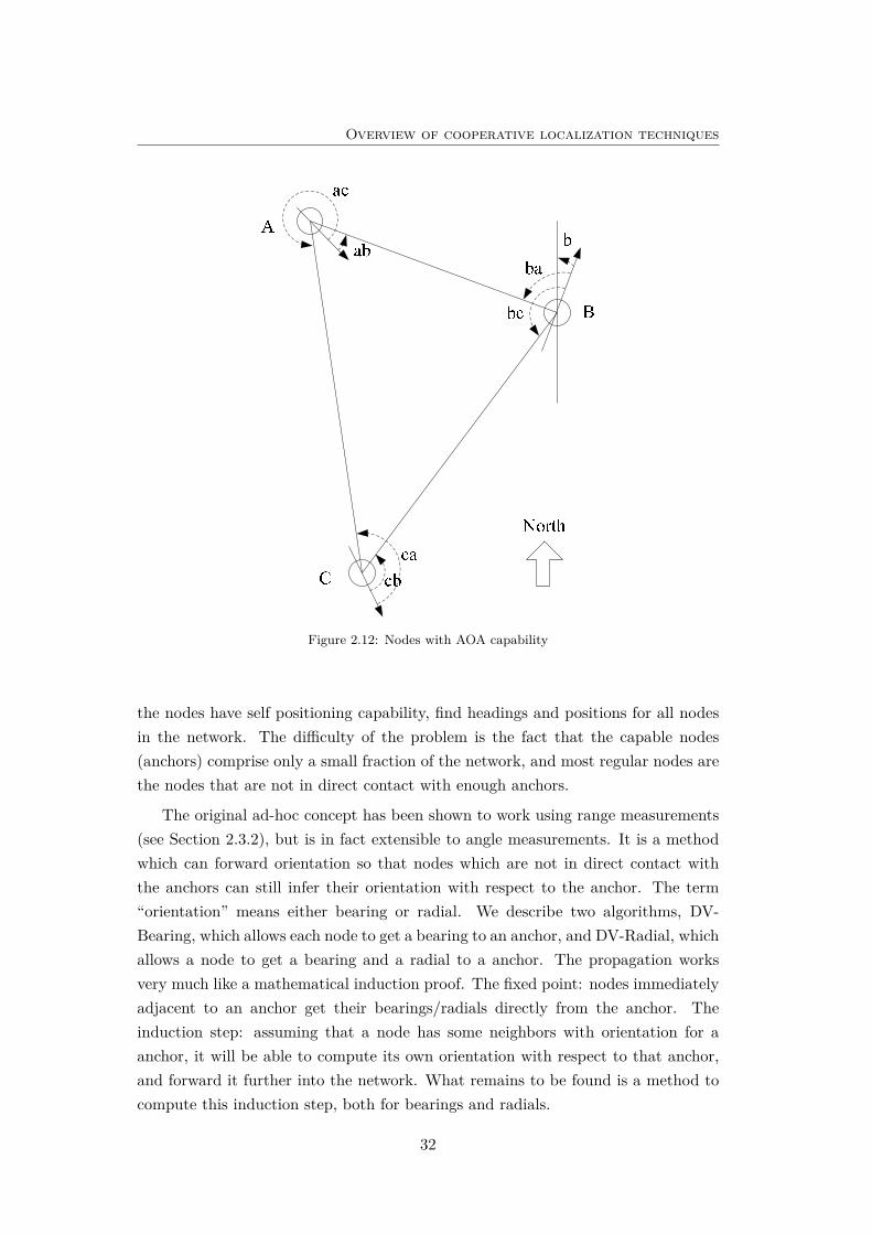
Overview of cooperative localization techniques
Figure 2.12: Nodes with AOA capability
the nodes have self positioning capability, find headings and positions for all nodesin the network. The difficulty of the problem is the fact that the capable nodes(anchors) comprise only a small fraction of the network, and most regular nodes arethe nodes that are not in direct contact with enough anchors.
The original ad-hoc concept has been shown to work using range measurements(see Section 2.3.2), but is in fact extensible to angle measurements. It is a methodwhich can forward orientation so that nodes which are not in direct contact withthe anchors can still infer their orientation with respect to the anchor. The term“orientation” means either bearing or radial. We describe two algorithms, DV-Bearing, which allows each node to get a bearing to an anchor, and DV-Radial, whichallows a node to get a bearing and a radial to a anchor. The propagation worksvery much like a mathematical induction proof. The fixed point: nodes immediatelyadjacent to an anchor get their bearings/radials directly from the anchor. Theinduction step: assuming that a node has some neighbors with orientation for aanchor, it will be able to compute its own orientation with respect to that anchor,and forward it further into the network. What remains to be found is a method tocompute this induction step, both for bearings and radials.
32
2.3 Deterministic localization techniques
Figure 2.13: Illustration of AOA algorithm: Node A infers its bearing to L using B’s and C’sbearings to L
The method is shown in Figure 2.13: assume node A knows its bearings toimmediate neighbors B and C (angles b and c), which in turn know their bearingsto a faraway landmark L. The problem is for A to find its bearing to L. If B andC are neighbors of each other, then A has the possibility to find all the angles intriangles ∆ABC and ∆BCL. This would allow A to find the angle LAC, whichyields the bearing of A with respect to L, as c+ LAC. Node A might accept anotherbearing to L from another pair of neighbors, if it involves less hops than the pairB-C. A then continues the process by forwarding its estimated bearing to L to itsneighbors which will help farther away nodes get their estimates for L. Once nodeA finds its bearings to at least three landmarks that are not on the same line or onthe same circle with A, it can infer its position using some triangulation procedurefor single-hop scenario.
If the radial method is to be used, a similar argument holds, with the differencethat now A needs to know, besides bearings of B and C to L, the radials of B andC from L. If the angle BLN (radial at B; ’N’ stands for ’north’) is also known, thenthe angle ALN (radial at A) can also be found since all angles in both triangles areknown. The actual downside for this method is in the increased communication -nodes B and C forward two values per landmark (bearing and radial) instead of justone, as in the bearing based method.
To conclude, the method we described infers position and orientation in an ad-hocnetwork where nodes can measure AOA from communication with their immediateneighbors. The assumption is that all unknown nodes have AOA capability andonly a fraction have self positioning capability. Two algorithms were described, DV-Bearing and DV-Radial. The advantages of the method are that it provides absolutecoordinates and absolute orientation, that it works well for disconnected networks,and does not require any additional infrastructure. Moreover, since the commu-
33
Overview of cooperative localization techniques
nication protocol can be localized, this algorithm is scalable to very large WSNs.Resulted positions have accuracy comparable to the range-based algorithms, andresulted orientations are usable for navigational and tracking purposes. However,high equipment cost makes this method impractical for WSN applications.
2.4 Probabilistic localization techniques
In contrast to deterministic methods [68, 82, 97, 100, 101, 109], probabilistic methods[8, 46, 48, 78, 118] take into account uncertainty of the measurements, so given thelikelihood of e.g., measured distance, and a prior PDF of the positions of all unknownnodes, they estimate the posterior PDFs of the positions of all unknown nodes.In order to find location estimates, it is sufficient to find either minimum meansquare estimate (MMSE), or maximum a posteriori (MAP) of this posterior PDF.These methods are also well-known as Bayesian methods. The main drawbackof the probabilistic methods is the high complexity, which makes these methodsunacceptable in low-power WSNs. Nevertheless, the particle-based approximation[2,32], and appropriate factorization using some message-passing method [77], makeprobabilistic methods acceptable for localization in WSN.
We provide here general framework for cooperative localization. Let us assumethat we have Ns sensors (Na anchors and Nu unknowns) scattered randomly in aplanar region, and denote the 2D location of sensor t by xt. The unknown node uobtains a noisy measurement dtu of its distance from node t with some probabilityPd(xt,xu):
dtu = ‖xt − xu‖+ vtu , vtu ∼ pv(dtu − ‖xt − xu‖ |Θtu) (2.21)
where, for noise vtu, we can assume a Gaussian distribution pv (with parameterΘtu = {µtu, σ2
tu}). However, it is straightforward to change it to any desired dis-tribution, e.g., an empirical distribution obtained by performing the experiments inthe deployment area.
The binary variable otu will indicate whether this observation is available or not:
otu ={
1, dtu observed,
0, otherwise.(2.22)
Finally, each sensor t has some prior distribution denoted pt(xt). This prior couldbe an uninformative one (i.e., with uniform distribution over the whole deploymentarea) for the unknowns and the Dirac Delta function for the anchors. Then, the
34
2.5 Summary
joint posterior PDF is given by:
p(x1, ..., xNu |{otu}, {dtu}) =∏(t,u)
p(otu |xt, xu )∏(t,u)
p(dtu |xt, xu )∏t
pt(xt) (2.23)
We also need to define probability of detection, from which we can draw variableotu. For large-scale WSNs, it is reasonable to assume that only a subset of pairwisedistances will be available, primarily between sensors which are located within thesome radius R. The ideal model of probability of detection is given by:
Pd(xt, xu) ={
1, for ‖xt − xu‖ ≤ R,0, otherwise.
(2.24)
Better approximations of Pd(xt, xu) can be obtained using real experiments in thedeployment area of interest, and is especially advisable for indoor scenarios. We canalso use the exponential model [46], which represents a better approximation:
Pd(xt, xu) = exp(−1
2 ‖xt − xu‖2 /R2
)(2.25)
Our goal is to compute the posterior marginal PDF p(xt, |{otu}, {dtu}) (for eachunknown node t) by marginalizing the joint posterior PDF, which is not tractablefor the localization problem. Therefore, we need to factorize the joint posteriorPDF using some message-passing method [77]. In addition, due to the presence ofnonlinear relationships and potentially non-Gaussian uncertainties, we should usea particle-based approximation [2, 32]. The best known method for this problem isNBP. It is recently used for cooperative localization in the static [46, 48] and themobile networks [99,118]. Detailed description of NBP, and a number of extensionswill be the main topic of Chapter 3.
2.5 Summary
In this chapter, we reviewed a number of cooperative WSN localization techniques.In particular, we described the standard measurement techniques (RSS, TOA/TDOA,AOA), deterministic localization methods (distance-based and connectivity-based),localization using AOA, and the general framework for probabilistic localization. Aswe can see, in the state-of-the-art there are a lot of deterministic methods withoutcapability to provide associated uncertainty online, especially in the case of non-Gaussian measurements, Therefore, further investigation of the probabilistic meth-ods will be the main topic of the following chapters of this thesis.
35

Overview of cooperative localization techniques
36
Chapter 3
Message passing methods forcooperative localization in loopynetworks
3.1 Introduction
Belief propagation (BP) [77, 121] is a way of organizing the global computation ofmarginal beliefs in terms of smaller local computations within the graph. It is oneof the best-known message passing methods for distributed inference in statisticalphysics, artificial intelligence, computer vision, localization, etc. The whole com-putation takes a time proportional to the number of links in the graph, which issignificantly less than the exponential time that would be required to compute mar-ginal probabilities naively. Therefore, BP is suitable for probabilistic cooperativeWSN localization described in Chapter 2. However, due to the presence of non-linear relationships and non-Gaussian uncertainties, the standard (parametric) BPis undesirable. Nevertheless, a particle-based approximation via nonparametric be-lief propagation (NBP), proposed by Ihler et al. [46, 48], makes BP acceptable forcooperative WSN localization.
However, in loopy networks NBP suffers from similar problems as standard BP,such as inaccurate beliefs and possible non-convergence. Few solutions for this prob-lem will be proposed in this chapter. We start with the description and analysis ofthe standard BP/NBP techniques, and also modified version of NBP, nonparametricboxed belief propagation (NBBP) [89,93]. Then, we propose four improved message-passing methods for loopy networks: nonparametric generalized belief propaga-tion (NGBP) based on junction tree (NGBP-JT) [90, 96], NGBP based on pseudo-
37
Message passing methods for cooperative localization in loopy networks
junction tree (NGBP-PJT) [92], NBP based on spanning trees (NBP-ST) [88, 91],and uniformly-reweighted NBP (URW-NBP) [79,95,119,120].
3.2 Belief propagation (BP)
In the standard BP algorithm [24,121], the belief at a node t (approximation of theposterior marginal PDF) is proportional to the product of the local evidence at thatnode ψt(xt), and all the messages coming into node t:
Mt(xt) = kψt(xt)∏u∈Gt
mut(xt) (3.1)
where xt is a state of node t, k is a normalization constant, and Gt denotes theneighbors of node t. The messages are determined by the message update rule:
mut(xt) =ˆxu
ψu(xu)ψtu(xt, xu)∏
g∈Gu\tmgu(xu)dxu (3.2)
where ψtu(xt, xu) is the pairwise potential between nodes t and u. On the right-hand side, there is a product over all messages going into node u except for the onecoming from node t. In other words, the message from node u to node t representsthe “opinion” of node u about the location of node t. The messages and beliefsare, of course, represented as PDFs, but not necessarily normalized. In practicalcomputation, one starts with nodes at the edge of the graph, and only computesa message when one has available all the messages required. It is easy to see [121]that each message needs to be computed only once for the graphs without loops.
For cooperative localization, we use an undirected graph [111] G = (V,E) con-sisting of a set of nodes or vertices V that are joined by a set of edges E. In orderto define an undirected graphical model (also knows as Markov random field), weplace at each node a random variable xs taking values in some space. In case oflocalization, this random variable represents the 2D location, and each edge repres-ents the measured distance. If we exclude the anchor nodes, the graph is obviouslyundirected.
The relationship between the graph and joint PDF may be quantified in termsof potential functions ψ which are defined over each of the graph’s cliques. A clique(C) is a subset of nodes such that for every two nodes in C, there exists an linkconnecting the two. So the joint PDF is given by:
p(x1, ..., xNu) ∝∏
cliquesC
ψC({xi : i ∈ C}) (3.3)
38
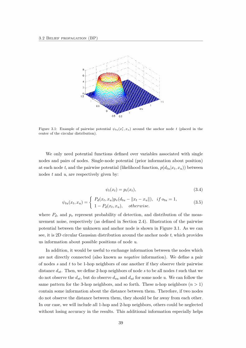
3.2 Belief propagation (BP)
Figure 3.1: Example of pairwise potential ψtu(x∗t , xu) around the anchor node t (placed in thecenter of the circular distribution).
We only need potential functions defined over variables associated with singlenodes and pairs of nodes. Single-node potential (prior information about position)at each node t, and the pairwise potential (likelihood function, p(dtu|xt, xu)) betweennodes t and u, are respectively given by:
ψt(xt) = pt(xt), (3.4)
ψtu(xt, xu) ={Pd(xt, xu)pv(dtu − ‖xt − xu‖), if otu = 1,1− Pd(xt, xu), otherwise.
(3.5)
where Pd, and pv represent probability of detection, and distribution of the meas-urement noise, respectively (as defined in Section 2.4). Illustration of the pairwisepotential between the unknown and anchor node is shown in Figure 3.1. As we cansee, it is 2D circular Gaussian distribution around the anchor node t, which providesus information about possible positions of node u.
In addition, it would be useful to exchange information between the nodes whichare not directly connected (also known as negative information). We define a pairof nodes s and t to be 1-hop neighbors of one another if they observe their pairwisedistance dst. Then, we define 2-hop neighbors of node s to be all nodes t such that wedo not observe the dst, but do observe dsu and dut for some node u. We can follow thesame pattern for the 3-hop neighbors, and so forth. These n-hop neighbors (n > 1)contain some information about the distance between them. Therefore, if two nodesdo not observe the distance between them, they should be far away from each other.In our case, we will include all 1-hop and 2-hop neighbors, others could be neglectedwithout losing accuracy in the results. This additional information especially helps
39
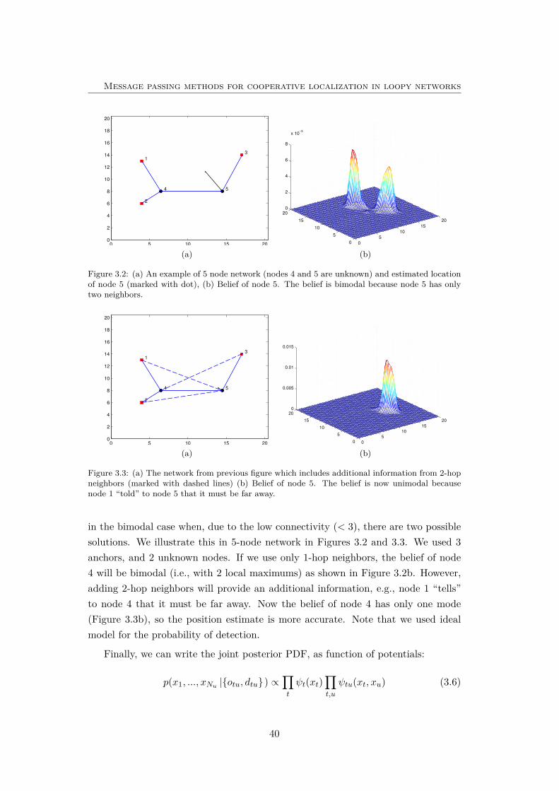
Message passing methods for cooperative localization in loopy networks
0 5 10 15 200
2
4
6
8
10
12
14
16
18
20
1
2
3
4 5
(a)0
5
10
15
20
0
5
10
15
20
0
2
4
6
8
x 10−3
(b)
Figure 3.2: (a) An example of 5 node network (nodes 4 and 5 are unknown) and estimated locationof node 5 (marked with dot), (b) Belief of node 5. The belief is bimodal because node 5 has onlytwo neighbors.
0 5 10 15 200
2
4
6
8
10
12
14
16
18
20
1
2
3
4 5
(a)0
5
10
15
20
0
5
10
15
20
0
0.005
0.01
0.015
(b)
Figure 3.3: (a) The network from previous figure which includes additional information from 2-hopneighbors (marked with dashed lines) (b) Belief of node 5. The belief is now unimodal becausenode 1 “told” to node 5 that it must be far away.
in the bimodal case when, due to the low connectivity (< 3), there are two possiblesolutions. We illustrate this in 5-node network in Figures 3.2 and 3.3. We used 3anchors, and 2 unknown nodes. If we use only 1-hop neighbors, the belief of node4 will be bimodal (i.e., with 2 local maximums) as shown in Figure 3.2b. However,adding 2-hop neighbors will provide an additional information, e.g., node 1 “tells”to node 4 that it must be far away. Now the belief of node 4 has only one mode(Figure 3.3b), so the position estimate is more accurate. Note that we used idealmodel for the probability of detection.
Finally, we can write the joint posterior PDF, as function of potentials:
p(x1, ..., xNu |{otu, dtu}) ∝∏t
ψt(xt)∏t,u
ψtu(xt, xu) (3.6)
40
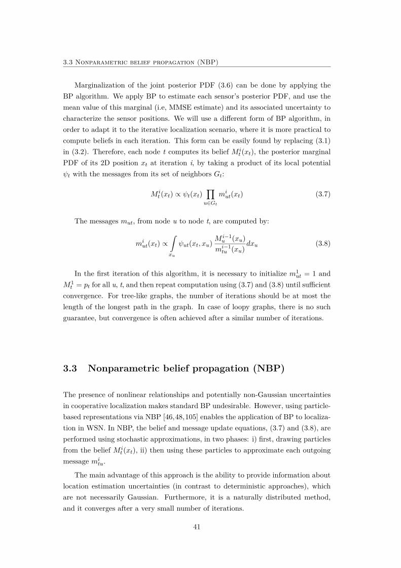
3.3 Nonparametric belief propagation (NBP)
Marginalization of the joint posterior PDF (3.6) can be done by applying theBP algorithm. We apply BP to estimate each sensor’s posterior PDF, and use themean value of this marginal (i.e, MMSE estimate) and its associated uncertainty tocharacterize the sensor positions. We will use a different form of BP algorithm, inorder to adapt it to the iterative localization scenario, where it is more practical tocompute beliefs in each iteration. This form can be easily found by replacing (3.1)in (3.2). Therefore, each node t computes its belief M i
t (xt), the posterior marginalPDF of its 2D position xt at iteration i, by taking a product of its local potentialψt with the messages from its set of neighbors Gt:
M it (xt) ∝ ψt(xt)
∏u∈Gt
miut(xt) (3.7)
The messages mut, from node u to node t, are computed by:
miut(xt) ∝
ˆxu
ψut(xt, xu) Mi−1u (xu)
mi−1tu (xu)
dxu (3.8)
In the first iteration of this algorithm, it is necessary to initialize m1ut = 1 and
M1t = pt for all u, t, and then repeat computation using (3.7) and (3.8) until sufficient
convergence. For tree-like graphs, the number of iterations should be at most thelength of the longest path in the graph. In case of loopy graphs, there is no suchguarantee, but convergence is often achieved after a similar number of iterations.
3.3 Nonparametric belief propagation (NBP)
The presence of nonlinear relationships and potentially non-Gaussian uncertaintiesin cooperative localization makes standard BP undesirable. However, using particle-based representations via NBP [46,48,105] enables the application of BP to localiza-tion in WSN. In NBP, the belief and message update equations, (3.7) and (3.8), areperformed using stochastic approximations, in two phases: i) first, drawing particlesfrom the belief M i
t (xt), ii) then using these particles to approximate each outgoingmessage mi
tu.
The main advantage of this approach is the ability to provide information aboutlocation estimation uncertainties (in contrast to deterministic approaches), whichare not necessarily Gaussian. Furthermore, it is a naturally distributed method,and it converges after a very small number of iterations.
41
Message passing methods for cooperative localization in loopy networks
3.3.1 Computing messages
Given N weighted particles {W j,it , Xj,i
t } from the beliefM it (xt) obtained at iteration
i, we can compute weighted particles of the outgoing BP message mitu. We first
consider the case of observed edges (1-hop) between unknown nodes. The distancemeasurement dtu provides information about how far sensor u is from sensor t, butno information about its relative direction (see Figure 3.1). To draw a particle ofthe message (xj,i+1
tu ), given the particle Xj,it which represents the position of sensor
t, we simply select a direction θj,i at random (i = 1), uniformly in the interval[0, 2π). However, starting from the second iteration, we can also include angularinformation [48] from the previous iteration using already computed beliefs. Wethen shift Xj,i
t in the direction of θj,i by an amount which represents the estimateddistance between nodes u and t (dtu + vj):
xj,i+1tu = Xj,i
t + (dtu + vj)[sin(θj,i) cos(θj,i)] (3.9)
For example, if node t is an anchor, the unknown node u, is located on noisy circlearound node t. That means that the particles from node u are distributed accordingto distribution shown in Figure 3.1. Assuming that there is detection between sensornodes t and u with probability Pd(xt, xu), the particles are weighted by the reminderof the message-update rule (3.8):
wj,i+1tu = Pd(Xi,j
t , xu) W j,it
miut(X
i,jt )
(3.10)
As we can see, for the denominator of (3.10), we need to know the parametricform of the message. We can approximate it using kernel density estimate (KDE)1.The optimal value for bandwidth hi+1
tu , can be obtained in a number of ways. Thesimplest technique is to apply the “rule of thumb” estimate [104]:
hi+1tu = N−
13 V ar({xi+1
tu }) (3.11)
It is also necessary to define messages coming from anchor nodes, which can befound using (3.8) and the belief of the anchor node x∗t (M i
t (xt) = δ(xt − x∗t )):
mi+1tu (xu) ∝ ψtu(x∗t , xu) (3.12)
1Approximation of the distribution p(x) : p(x) =∑
jwjKh(x− xj) given a Kernel Kh(x).
The most common kernel function (Kh) is the spherically symmetric Gaussian kernel: Kh(x) =N(x, 0, hI), where bandwidth h controls the variance [48,104].
42
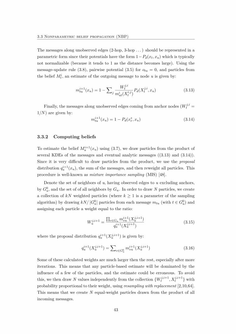
3.3 Nonparametric belief propagation (NBP)
The messages along unobserved edges (2-hop, 3-hop . . . ) should be represented in aparametric form since their potentials have the form 1−Pd(xt, xu) which is typicallynot normalizable (because it tends to 1 as the distance becomes large). Using themessage-update rule (3.8), pairwise potential (3.5) for otu = 0, and particles fromthe belief M i
t , an estimate of the outgoing message to node u is given by:
mi+1tu (xu) = 1−
∑j
W j,it
miut(X
i,jt )
Pd(Xj,it , xu) (3.13)
Finally, the messages along unobserved edges coming from anchor nodes (W j,it =
1/N) are given by:mi+1tu (xu) = 1− Pd(x∗t , xu) (3.14)
3.3.2 Computing beliefs
To estimate the belief M i+1u (xu) using (3.7), we draw particles from the product of
several KDEs of the messages and eventual analytic messages ((3.13) and (3.14)).Since it is very difficult to draw particles from the product, we use the proposaldistribution qi+1
u (xu), the sum of the messages, and then reweight all particles. Thisprocedure is well-known as mixture importance sampling (MIS) [48].
Denote the set of neighbors of u, having observed edges to u excluding anchors,by G0
u, and the set of of all neighbors by Gu. In order to draw N particles, we createa collection of kN weighted particles (where k ≥ 1 is a parameter of the samplingalgorithm) by drawing kN/
∣∣G0u
∣∣ particles from each message mtu (with t ∈ G0u) and
assigning each particle a weight equal to the ratio:
W j,i+1u =
∏v∈Gum
i+1vu (Xj,i+1
u )qi+1u (Xj,i+1
u )(3.15)
where the proposal distribution qi+1u (Xj,i+1
u ) is given by:
qi+1u (Xj,i+1
u ) =∑
v∈G0u
mi+1vu (Xj,i+1
u ) (3.16)
Some of these calculated weights are much larger then the rest, especially after moreiterations. This means that any particle-based estimate will be dominated by theinfluence of a few of the particles, and the estimate could be erroneous. To avoidthis, we then draw N values independently from the collection {W j,i+1
t , Xj,i+1t } with
probability proportional to their weight, using resampling with replacement [2,10,64].This means that we create N equal-weight particles drawn from the product of allincoming messages.
43
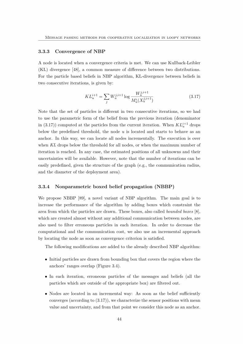
Message passing methods for cooperative localization in loopy networks
3.3.3 Convergence of NBP
A node is located when a convergence criteria is met. We can use Kullback-Leibler(KL) divergence [48], a common measure of difference between two distributions.For the particle based beliefs in NBP algorithm, KL-divergence between beliefs intwo consecutive iterations, is given by:
KLi+1u =
∑j
W j,i+1u log W j,i+1
u
M iu(Xj,i+1
u )(3.17)
Note that the set of particles is different in two consecutive iterations, so we hadto use the parametric form of the belief from the previous iteration (denominatorin (3.17)) computed at the particles from the current iteration. When KLi+1
u dropsbelow the predefined threshold, the node u is located and starts to behave as ananchor. In this way, we can locate all nodes incrementally. The execution is overwhen KL drops below the threshold for all nodes, or when the maximum number ofiteration is reached. In any case, the estimated positions of all unknowns and theiruncertainties will be available. However, note that the number of iterations can beeasily predefined, given the structure of the graph (e.g., the communication radius,and the diameter of the deployment area).
3.3.4 Nonparametric boxed belief propagation (NBBP)
We propose NBBP [89], a novel variant of NBP algorithm. The main goal is toincrease the performance of the algorithm by adding boxes which constraint thearea from which the particles are drawn. These boxes, also called bounded boxes [8],which are created almost without any additional communication between nodes, arealso used to filter erroneous particles in each iteration. In order to decrease thecomputational and the communication cost, we also use an incremental approachby locating the node as soon as convergence criterion is satisfied.
The following modifications are added to the already described NBP algorithm:
• Initial particles are drawn from bounding box that covers the region where theanchors’ ranges overlap (Figure 3.4).
• In each iteration, erroneous particles of the messages and beliefs (all theparticles which are outside of the appropriate box) are filtered out.
• Nodes are located in an incremental way: As soon as the belief sufficientlyconverges (according to (3.17)), we characterize the sensor positions with meanvalue and uncertainty, and from that point we consider this node as an anchor.
44
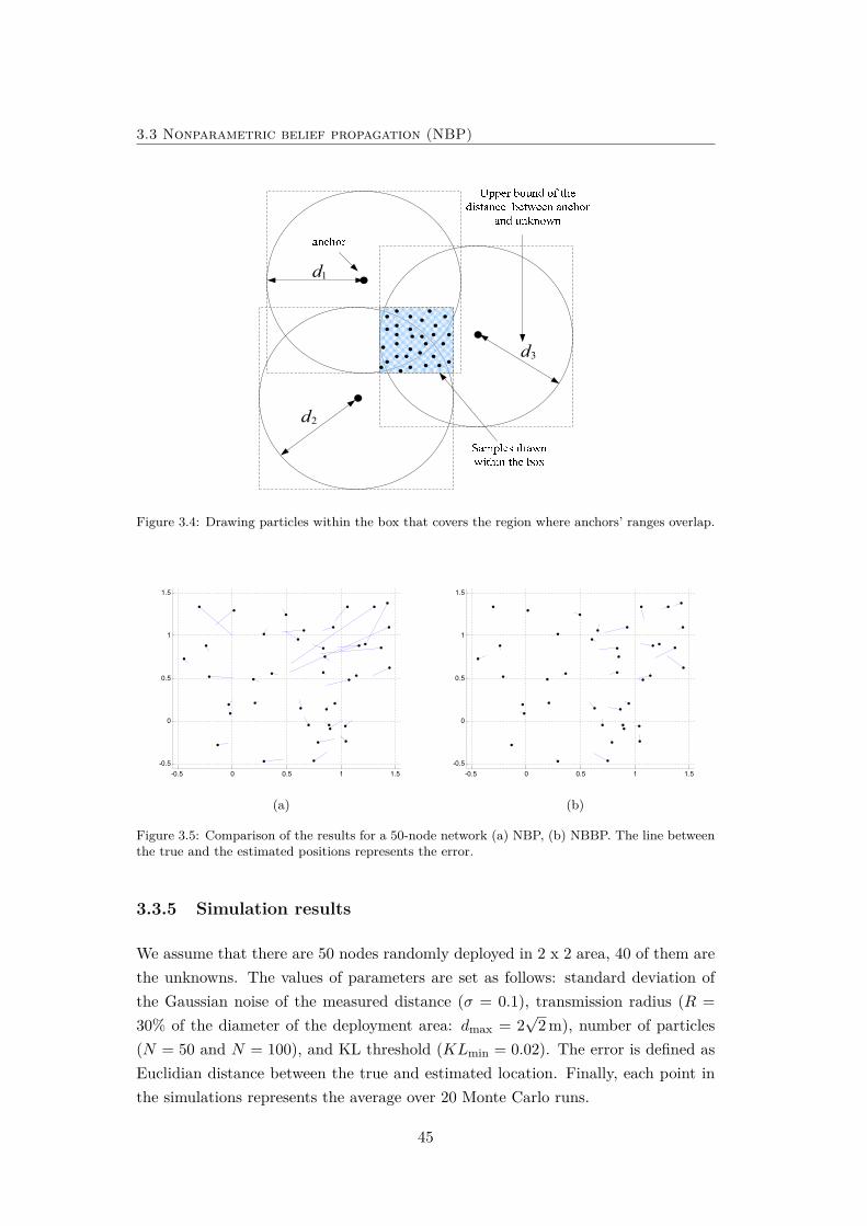
3.3 Nonparametric belief propagation (NBP)
1d
2d
3d
Figure 3.4: Drawing particles within the box that covers the region where anchors’ ranges overlap.
-0.5 0 0.5 1 1.5-0.5
0
0.5
1
1.5
(a)
-0.5 0 0.5 1 1.5-0.5
0
0.5
1
1.5
(b)
Figure 3.5: Comparison of the results for a 50-node network (a) NBP, (b) NBBP. The line betweenthe true and the estimated positions represents the error.
3.3.5 Simulation results
We assume that there are 50 nodes randomly deployed in 2 x 2 area, 40 of them arethe unknowns. The values of parameters are set as follows: standard deviation ofthe Gaussian noise of the measured distance (σ = 0.1), transmission radius (R =30% of the diameter of the deployment area: dmax = 2
√2 m), number of particles
(N = 50 and N = 100), and KL threshold (KLmin = 0.02). The error is defined asEuclidian distance between the true and estimated location. Finally, each point inthe simulations represents the average over 20 Monte Carlo runs.
45
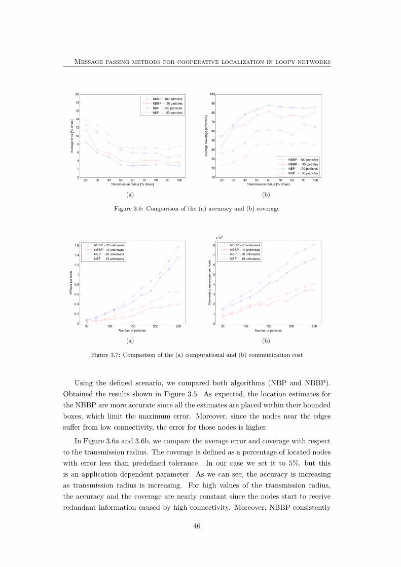
Message passing methods for cooperative localization in loopy networks
20 30 40 50 60 70 80 90 1000
2
4
6
8
10
12
14
16
18
20
Transmission radius [% dmax]
Ave
rage
erro
r [%
dm
ax]
NBBP - 100 particlesNBBP - 50 particlesNBP - 100 particlesNBP - 50 particles
(a)
20 30 40 50 60 70 80 90 10010
20
30
40
50
60
70
80
90
100
Transmission radius [% dmax]
Ave
rage
cov
erag
e (e
rror<
5%)
NBBP - 100 particlesNBBP - 50 particlesNBP - 100 particlesNBP - 50 particles
(b)
Figure 3.6: Comparison of the (a) accuracy and (b) coverage
50 100 150 200 2500
0.2
0.4
0.6
0.8
1
1.2
1.4
1.6
Number of particles
MFl
ops
per n
ode
NBBP - 20 unknownsNBBP - 10 unknownsNBP - 20 unknownsNBP - 10 unknowns
(a)
50 100 150 200 2500
1
2
3
4
5
6
7
8
x 104
Number of particles
Ele
men
tary
mes
sage
s pe
r nod
e
NBBP - 20 unknownsNBBP - 10 unknownsNBP - 20 unknownsNBP - 10 unknowns
(b)
Figure 3.7: Comparison of the (a) computational and (b) communication cost
Using the defined scenario, we compared both algorithms (NBP and NBBP).Obtained the results shown in Figure 3.5. As expected, the location estimates forthe NBBP are more accurate since all the estimates are placed within their boundedboxes, which limit the maximum error. Moreover, since the nodes near the edgessuffer from low connectivity, the error for those nodes is higher.
In Figure 3.6a and 3.6b, we compare the average error and coverage with respectto the transmission radius. The coverage is defined as a percentage of located nodeswith error less than predefined tolerance. In our case we set it to 5%, but thisis an application dependent parameter. As we can see, the accuracy is increasingas transmission radius is increasing. For high values of the transmission radius,the accuracy and the coverage are nearly constant since the nodes start to receiveredundant information caused by high connectivity. Moreover, NBBP consistently
46
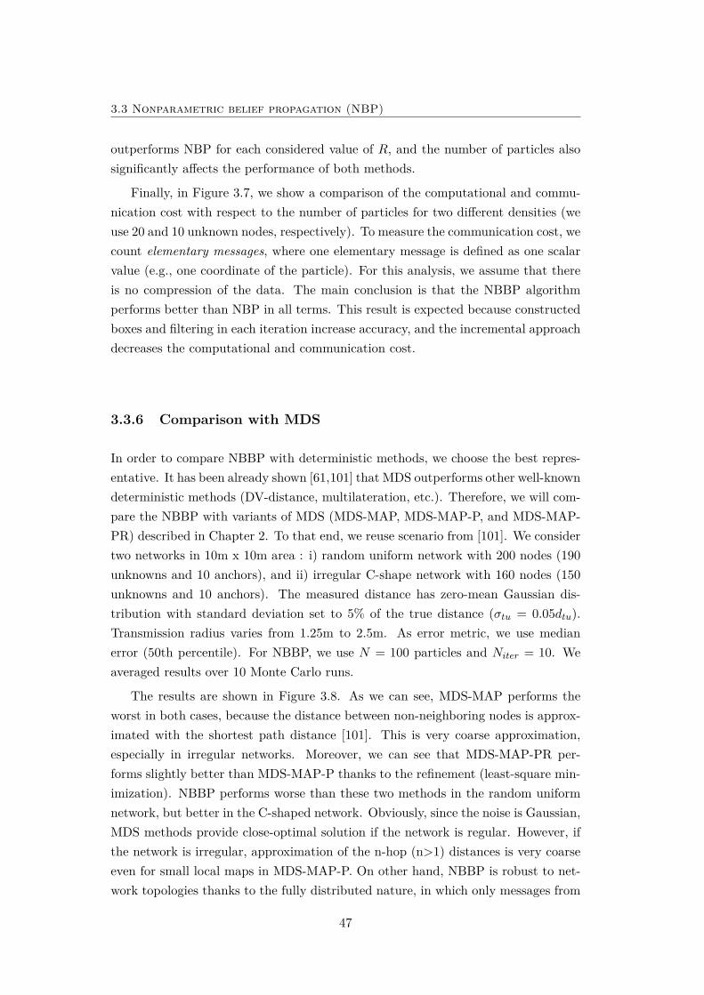
3.3 Nonparametric belief propagation (NBP)
outperforms NBP for each considered value of R, and the number of particles alsosignificantly affects the performance of both methods.
Finally, in Figure 3.7, we show a comparison of the computational and commu-nication cost with respect to the number of particles for two different densities (weuse 20 and 10 unknown nodes, respectively). To measure the communication cost, wecount elementary messages, where one elementary message is defined as one scalarvalue (e.g., one coordinate of the particle). For this analysis, we assume that thereis no compression of the data. The main conclusion is that the NBBP algorithmperforms better than NBP in all terms. This result is expected because constructedboxes and filtering in each iteration increase accuracy, and the incremental approachdecreases the computational and communication cost.
3.3.6 Comparison with MDS
In order to compare NBBP with deterministic methods, we choose the best repres-entative. It has been already shown [61,101] that MDS outperforms other well-knowndeterministic methods (DV-distance, multilateration, etc.). Therefore, we will com-pare the NBBP with variants of MDS (MDS-MAP, MDS-MAP-P, and MDS-MAP-PR) described in Chapter 2. To that end, we reuse scenario from [101]. We considertwo networks in 10m x 10m area : i) random uniform network with 200 nodes (190unknowns and 10 anchors), and ii) irregular C-shape network with 160 nodes (150unknowns and 10 anchors). The measured distance has zero-mean Gaussian dis-tribution with standard deviation set to 5% of the true distance (σtu = 0.05dtu).Transmission radius varies from 1.25m to 2.5m. As error metric, we use medianerror (50th percentile). For NBBP, we use N = 100 particles and Niter = 10. Weaveraged results over 10 Monte Carlo runs.
The results are shown in Figure 3.8. As we can see, MDS-MAP performs theworst in both cases, because the distance between non-neighboring nodes is approx-imated with the shortest path distance [101]. This is very coarse approximation,especially in irregular networks. Moreover, we can see that MDS-MAP-PR per-forms slightly better than MDS-MAP-P thanks to the refinement (least-square min-imization). NBBP performs worse than these two methods in the random uniformnetwork, but better in the C-shaped network. Obviously, since the noise is Gaussian,MDS methods provide close-optimal solution if the network is regular. However, ifthe network is irregular, approximation of the n-hop (n>1) distances is very coarseeven for small local maps in MDS-MAP-P. On other hand, NBBP is robust to net-work topologies thanks to the fully distributed nature, in which only messages from
47
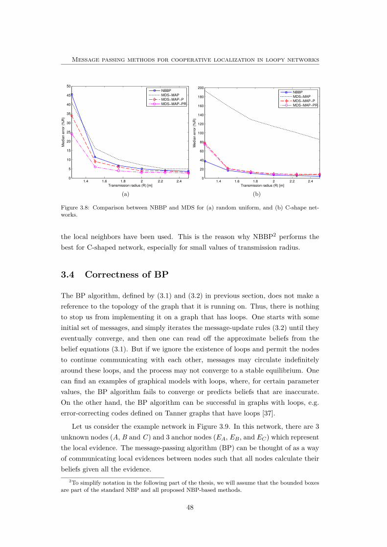
Message passing methods for cooperative localization in loopy networks
1.4 1.6 1.8 2 2.2 2.40
5
10
15
20
25
30
35
40
45
50
Transmission radius (R) [m]
Media
n e
rror
(%R
)
NBBP
MDS−MAP
MDS−MAP−P
MDS−MAP−PR
(a)
1.4 1.6 1.8 2 2.2 2.40
20
40
60
80
100
120
140
160
180
200
Transmission radius (R) [m]
Me
dia
n e
rro
r (%
R)
NBBP
MDS−MAP
MDS−MAP−P
MDS−MAP−PR
(b)
Figure 3.8: Comparison between NBBP and MDS for (a) random uniform, and (b) C-shape net-works.
the local neighbors have been used. This is the reason why NBBP2 performs thebest for C-shaped network, especially for small values of transmission radius.
3.4 Correctness of BP
The BP algorithm, defined by (3.1) and (3.2) in previous section, does not make areference to the topology of the graph that it is running on. Thus, there is nothingto stop us from implementing it on a graph that has loops. One starts with someinitial set of messages, and simply iterates the message-update rules (3.2) until theyeventually converge, and then one can read off the approximate beliefs from thebelief equations (3.1). But if we ignore the existence of loops and permit the nodesto continue communicating with each other, messages may circulate indefinitelyaround these loops, and the process may not converge to a stable equilibrium. Onecan find an examples of graphical models with loops, where, for certain parametervalues, the BP algorithm fails to converge or predicts beliefs that are inaccurate.On the other hand, the BP algorithm can be successful in graphs with loops, e.g.error-correcting codes defined on Tanner graphs that have loops [37].
Let us consider the example network in Figure 3.9. In this network, there are 3unknown nodes (A, B and C ) and 3 anchor nodes (EA, EB, and EC) which representthe local evidence. The message-passing algorithm (BP) can be thought of as a wayof communicating local evidences between nodes such that all nodes calculate theirbeliefs given all the evidence.
2To simplify notation in the following part of the thesis, we will assume that the bounded boxesare part of the standard NBP and all proposed NBP-based methods.
48
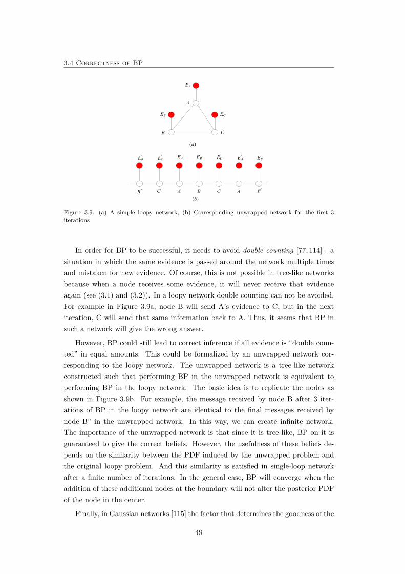
3.4 Correctness of BP
A
B C
AE
BE CE
CE'CE AE '
AEBE''BE '
BE
C'C''B BA 'A 'B
( )a
( )b
Figure 3.9: (a) A simple loopy network, (b) Corresponding unwrapped network for the first 3iterations
In order for BP to be successful, it needs to avoid double counting [77, 114] - asituation in which the same evidence is passed around the network multiple timesand mistaken for new evidence. Of course, this is not possible in tree-like networksbecause when a node receives some evidence, it will never receive that evidenceagain (see (3.1) and (3.2)). In a loopy network double counting can not be avoided.For example in Figure 3.9a, node B will send A’s evidence to C, but in the nextiteration, C will send that same information back to A. Thus, it seems that BP insuch a network will give the wrong answer.
However, BP could still lead to correct inference if all evidence is “double coun-ted” in equal amounts. This could be formalized by an unwrapped network cor-responding to the loopy network. The unwrapped network is a tree-like networkconstructed such that performing BP in the unwrapped network is equivalent toperforming BP in the loopy network. The basic idea is to replicate the nodes asshown in Figure 3.9b. For example, the message received by node B after 3 iter-ations of BP in the loopy network are identical to the final messages received bynode B” in the unwrapped network. In this way, we can create infinite network.The importance of the unwrapped network is that since it is tree-like, BP on it isguaranteed to give the correct beliefs. However, the usefulness of these beliefs de-pends on the similarity between the PDF induced by the unwrapped problem andthe original loopy problem. And this similarity is satisfied in single-loop networkafter a finite number of iterations. In the general case, BP will converge when theaddition of these additional nodes at the boundary will not alter the posterior PDFof the node in the center.
Finally, in Gaussian networks [115] the factor that determines the goodness of the
49
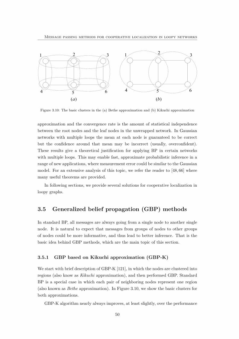
Message passing methods for cooperative localization in loopy networks
1 2 3
4 5 6
1 2 3
4 5 6
( )a ( )b
Figure 3.10: The basic clusters in the (a) Bethe approximation and (b) Kikuchi approximation
approximation and the convergence rate is the amount of statistical independencebetween the root nodes and the leaf nodes in the unwrapped network. In Gaussiannetworks with multiple loops the mean at each node is guaranteed to be correctbut the confidence around that mean may be incorrect (usually, overconfident).These results give a theoretical justification for applying BP in certain networkswith multiple loops. This may enable fast, approximate probabilistic inference in arange of new applications, where measurement error could be similar to the Gaussianmodel. For an extensive analysis of this topic, we refer the reader to [48, 66] wheremany useful theorems are provided.
In following sections, we provide several solutions for cooperative localization inloopy graphs.
3.5 Generalized belief propagation (GBP) methods
In standard BP, all messages are always going from a single node to another singlenode. It is natural to expect that messages from groups of nodes to other groupsof nodes could be more informative, and thus lead to better inference. That is thebasic idea behind GBP methods, which are the main topic of this section.
3.5.1 GBP based on Kikuchi approximation (GBP-K)
We start with brief description of GBP-K [121], in which the nodes are clustered intoregions (also know as Kikuchi approximation), and then performed GBP. StandardBP is a special case in which each pair of neighboring nodes represent one region(also known as Bethe approximation). In Figure 3.10, we show the basic clusters forboth approximations.
GBP-K algorithm nearly always improves, at least slightly, over the performance
50
3.5 Generalized belief propagation (GBP) methods
of standard BP, and it can significantly outperform standard BP if the graphicalmodel under consideration has only short loops. However, the complexity of GBP-K grows exponentially with the size of the basic clusters that are chosen. If weinclude all loops as the basic clusters, the GBP-K algorithm is exact, but computa-tionally unacceptable. This is the reason why this method is not appropriate for thelocalization problem at hand. For the detailed description of the GBP-K methodand its variations, the reader is referred to [121].
3.5.2 GBP based on junction-tree (GBP-JT)
GBP-JT is a standard method for exact inference in graphical model. That meansthat all posterior marginals will provide the true information about uncertainty ofnode estimates. This method can be derived using the elimination procedure [52].The graph is first triangulated (i.e. “virtual” edges are added so that every loop oflength more than 3 has a chord). Given a triangulated graph, with cliques Ci andpotentials ψCi(xCi), and given the corresponding junction tree (JT), which defineslinks between the cliques, we send the following message from clique Ci to clique Cjby the message update rule:
mij(xSij ) =∑Ci\Sij
ψCi(xCi)∏
k∈Gi\jmki(xSki) (3.18)
where Sij = Ci ∩ Cj , and where Gi are the neighbors of clique Ci in the JT. Thebelief at clique Ci is proportional to the product of the local evidence at that cliqueand all the messages coming into clique i:
Mi(xCi) = kψCi(xCi)∏j∈Gi
mji(xSji) (3.19)
Beliefs for single nodes can be obtained via further marginalization:
Mi(xi) =∑Ci\i
Mi(xCi) for i ∈ Ci (3.20)
Equations (3.18), (3.19), and (3.20) represent GBP-JT algorithm which is validfor arbitrary graphs. Note that in case of continuous variables, summation have to bereplaced by integration. The BP algorithm defined with (3.1) and (3.2) is a specialcase of GBP-JT, obtaining by noting that the original tree is already triangulated,and has only pairs of nodes as cliques. In that case, sets Sij are single nodes, andmarginalization using (3.20) is unnecessary.
We also need to define clique potential ψCi , which is given as a product of all
51
Message passing methods for cooperative localization in loopy networks
single-node and pairwise potentials. The potentials of 2-node clique Ci(t, u) and3-node clique Cj(t, u, v) are, respectively, given by:
ψCi(xCi) = ψtu(xt, xu)ψt(xt)ψu(xu) (3.21)
ψCj (xCj ) = ψtu(xt, xu)ψtv(xt, xv)ψuv(xu, xv)ψt(xt)ψu(xu)ψv(xv) (3.22)
The potentials of larger cliques can be defined in analog way. The single-node poten-tial ψt and pairwise potential ψtu are given by equations (3.4) and (3.5), respectively.If the edge (t, u) is triangulated, we set ψtu = 1. To provide better understandingof GBP-JT, we analyze an example in Appendix A.
As in case of BP, because of the presence of nonlinear relationships, and poten-tially highly non-Gaussian uncertainties, we need to apply nonparametric approx-imation of GBP-JT method (NGBP-JT). We skip the description since the generalframework will be provided for the NGBP-PJT method in Section 3.5.4 (which usesthe same nonparametric approximation as NGBP-JT). Detailed example can be alsofound in [90].
3.5.3 GBP based on pseudo-junction-tree (GBP-PJT)
There remained two main problems of GBP-JT method: i) how to efficiently formthe JT in an arbitrary network, and ii) how to decrease the effective dimensionality ofthe particles. To address these problem, we propose GBP-PJT. The main differencecomparing with GBP-JT is the formation of pseudo-junction tree (PJT), whichrepresents the approximated JT based on thin graph (TG). In addition, in orderto decrease the number of high-dimensional particles, we use improved importancedensity function, and also propose dimensionality reduction of the messages. Asby-product, we also propose NBP based on TG (NBP-TG), cheaper variant of NBP,which runs on the same graph as NGBP-PJT.
JT formation
JT is a clique tree based on triangulated graph [52,55], i.e., a graph with additional“virtual” edges so that every loop of length more than 3 has a chord. In triangulatedgraph, each 3-node loop (which is not subset of any larger clique) represents 3-node clique, and each edge (which is not subset of any 3-node clique) represents2-node clique. Larger cliques (> 3) should be avoided, but this is not possible inmost graphs, even with optimal triangulation procedure. Using these cliques ashypernodes, we can define a cluster graph [55] by connecting each pair of the cliqueswith minimum one common node (i.e., non-empty intersection). Using cluster graph,
52
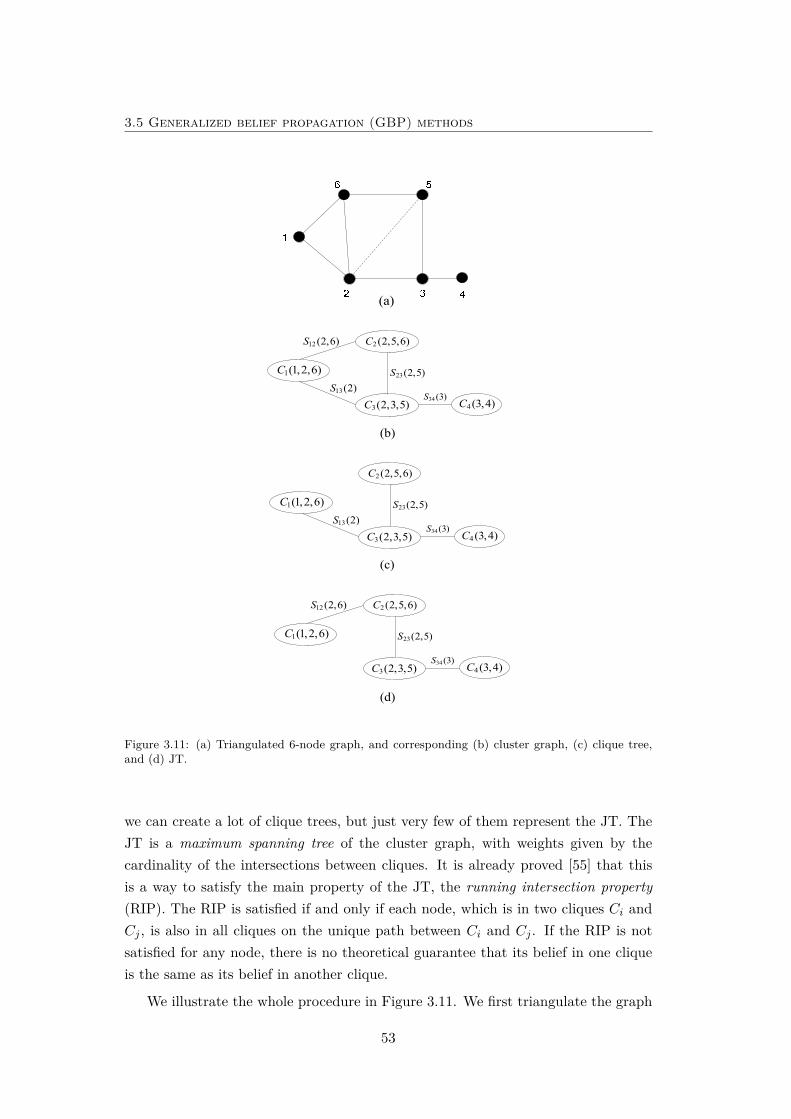
3.5 Generalized belief propagation (GBP) methods
(a)
1(1,2,6)C
2(2,5,6)C
3(2,3,5)C 4 (3,4)C34 (3)S
12 (2,6)S
23(2,5)S
(d)
1(1,2,6)C
2(2,5,6)C
3(2,3,5)C 4 (3,4)C34 (3)S13(2)S
12 (2,6)S
23(2,5)S
(b)
1(1,2,6)C
2(2,5,6)C
3(2,3,5)C 4 (3,4)C34 (3)S13(2)S
23(2,5)S
(c)
Figure 3.11: (a) Triangulated 6-node graph, and corresponding (b) cluster graph, (c) clique tree,and (d) JT.
we can create a lot of clique trees, but just very few of them represent the JT. TheJT is a maximum spanning tree of the cluster graph, with weights given by thecardinality of the intersections between cliques. It is already proved [55] that thisis a way to satisfy the main property of the JT, the running intersection property(RIP). The RIP is satisfied if and only if each node, which is in two cliques Ci andCj , is also in all cliques on the unique path between Ci and Cj . If the RIP is notsatisfied for any node, there is no theoretical guarantee that its belief in one cliqueis the same as its belief in another clique.
We illustrate the whole procedure in Figure 3.11. We first triangulate the graph
53
Message passing methods for cooperative localization in loopy networks
by adding the edge between nodes 2 and 5 (Figure 3.11a). Then we form thecluster graph (Figure 3.11b) with cliques Ci(t, u, v) and separator sets Sij(q, r) (Sij =Ci ∩ Cj), where t, u, v are the nodes in the clique, and q, r are the separatornodes. Finally, any spanning tree (ST) represents the clique tree like in Figure 3.11cand Figure 3.11d. The tree in Figure 3.11d is maximum ST (|S12| > |S13|), so itrepresents the JT of the initial graph. Note that the tree in Figure 3.11c does notsatisfy RIP since the node 6, which is in C1 and C2, is not in C3.
The described procedure represents the exact formation of the JT, also knownas chordal graph method. The main problem of this approach is the triangulationphase. Finding, a minimum triangulation, i.e., one where the largest clique hasminimum size, is NP-hard problem due to the number of permutations that mustbe checked. Of course, there exist approximate methods (e.g., [45]) which are lessexpensive, but, according to authors, still too costly. For more details, see Chapter10 in [55].
PJT formation
Due to the high complexity of the optimal JT formation, it is necessary to find someapproximation that will be suitable for the localization problem. Therefore, we tryto achieve the following:
(a) The number of cliques should be reasonable (i.e., in the order of the number ofnodes).
(b) In order to reduce the dimensionality of the problem, each clique will includeno more than 3 nodes.
(c) Since the triangulation is expensive procedure, we are going to avoid it, even ifit causes the break of RIP for the small percentage of the nodes.
After these approximations, the final result represents, strictly speaking, theclique tree. However, since it is very close to the JT (measured by percentage of thenodes that satisfies RIP), we name it pseudo-junction tree (PJT).
In order to satisfy the conditions (a) and (b), we need to decrease the number ofedges in the graph by formation of thin graph (TG). That can be easily done usingmodified version of breadth first search (BFS) method. Standard BFS method [7]begins at randomly chosen root node and explores all the neighboring nodes. Theneach of those neighbors explores their unexplored neighbors, and so on, until all thenodes are explored. In this way, there will not be a loop in the graph because all thenodes will be explored just once. Thus, the final result of BFS is a ST. The worst
54

3.5 Generalized belief propagation (GBP) methods
Algorithm 3 Searching for TG and cliques using modified BFS method1: Input: node list Q and root node root2: Copy to node lists: Nodes,NewV isit← Q3: Set current root: r ← root4: Create list of neighbors for all nodes n ∈ Q: Gn5: while Nodes is not empty do6: for all nodes t ∈ Gr do7: if t ∈ Nodes then8: Remove t from Nodes9: Insert t in WaitingRoots
10: Insert drt in T11: else if drt /∈ T and r ∈ NewV isit then12: Insert drt in T13: Remove r from NewV isit14: Create 3-node cliques:15: for all q ∈ PreviousRoots do16: if {drq, dtq} ∈ T then17: C3nodes ← {r, t, q}18: end if19: end for20: end if21: end for22: Insert r in PreviousRoots23: Set current root: r ← first unused node from
WaitingRoots24: end while25: Create 2-node cliques C2nodes: each edge in T which is not subset of C3nodes
26: Output: thin graph {Q,T} and cliques C = C2nodes ∪ C3nodes
case complexity is O(v + e), where v is the number of nodes and e is the number ofedges in the graph, since every node and every edge will be explored in the worstcase.
Nevertheless, a ST is very coarse approximation of the original graph since itexcludes a lot of edges from the graph. For example, in any ST, one communicationfailure breaks the graph into the two parts. As a consequence, we need more STsin order to have reasonable accurate inference in graphical models (this idea willbe used in Section 3.6). Therefore, we modify standard BFS method by permittingeach root node to make additional visit to the node that was already visited by someof the previous roots. All edges found by the first and the second visit, together withall the nodes from the original graph, represent the TG. In addition, the second visitwill automatically form a loop, so we use it to form 3-node clique. The 2-node cliquescan be found easily by taking all the edges that appear in TG, which are not alreadysubset of any a 3-node clique. The worst complexity is O(v+e+v · (v−1)) ≈ O(v2),
55
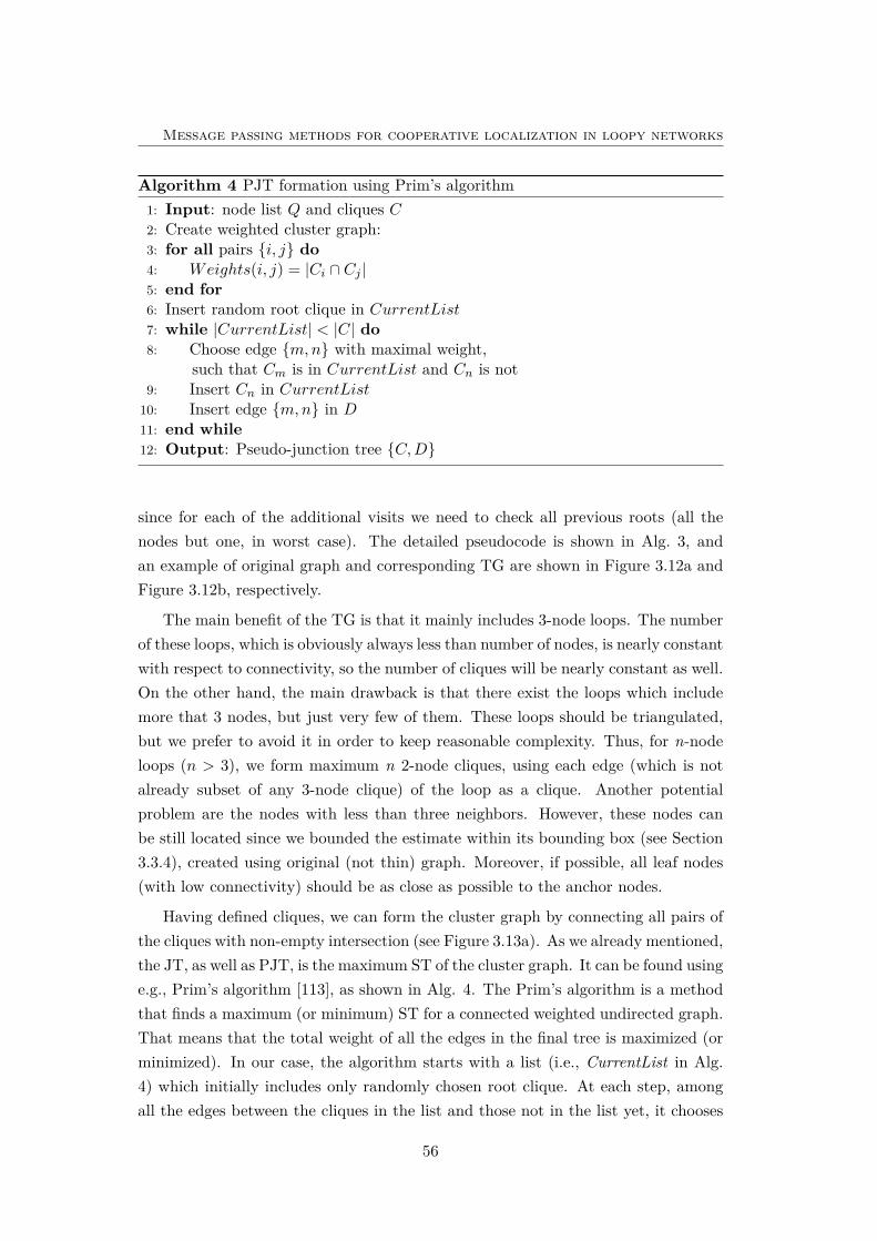
Message passing methods for cooperative localization in loopy networks
Algorithm 4 PJT formation using Prim’s algorithm1: Input: node list Q and cliques C2: Create weighted cluster graph:3: for all pairs {i, j} do4: Weights(i, j) = |Ci ∩ Cj |5: end for6: Insert random root clique in CurrentList7: while |CurrentList| < |C| do8: Choose edge {m,n} with maximal weight,
such that Cm is in CurrentList and Cn is not9: Insert Cn in CurrentList
10: Insert edge {m,n} in D11: end while12: Output: Pseudo-junction tree {C,D}
since for each of the additional visits we need to check all previous roots (all thenodes but one, in worst case). The detailed pseudocode is shown in Alg. 3, andan example of original graph and corresponding TG are shown in Figure 3.12a andFigure 3.12b, respectively.
The main benefit of the TG is that it mainly includes 3-node loops. The numberof these loops, which is obviously always less than number of nodes, is nearly constantwith respect to connectivity, so the number of cliques will be nearly constant as well.On the other hand, the main drawback is that there exist the loops which includemore that 3 nodes, but just very few of them. These loops should be triangulated,but we prefer to avoid it in order to keep reasonable complexity. Thus, for n-nodeloops (n > 3), we form maximum n 2-node cliques, using each edge (which is notalready subset of any 3-node clique) of the loop as a clique. Another potentialproblem are the nodes with less than three neighbors. However, these nodes canbe still located since we bounded the estimate within its bounding box (see Section3.3.4), created using original (not thin) graph. Moreover, if possible, all leaf nodes(with low connectivity) should be as close as possible to the anchor nodes.
Having defined cliques, we can form the cluster graph by connecting all pairs ofthe cliques with non-empty intersection (see Figure 3.13a). As we already mentioned,the JT, as well as PJT, is the maximum ST of the cluster graph. It can be found usinge.g., Prim’s algorithm [113], as shown in Alg. 4. The Prim’s algorithm is a methodthat finds a maximum (or minimum) ST for a connected weighted undirected graph.That means that the total weight of all the edges in the final tree is maximized (orminimized). In our case, the algorithm starts with a list (i.e., CurrentList in Alg.4) which initially includes only randomly chosen root clique. At each step, amongall the edges between the cliques in the list and those not in the list yet, it chooses
56
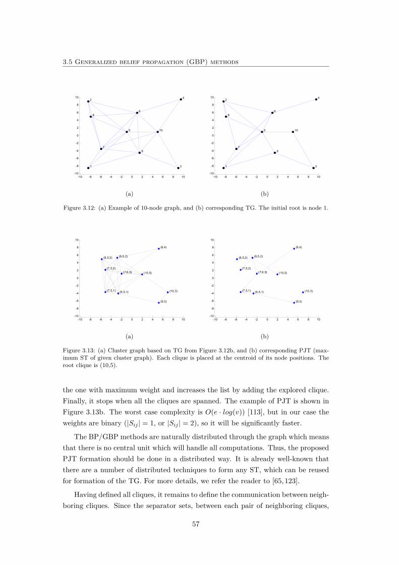
3.5 Generalized belief propagation (GBP) methods
-10 -8 -6 -4 -2 0 2 4 6 8 10-10
-8
-6
-4
-2
0
2
4
6
8
10
1
2
3
4
5
6
7
8
9
10
(a)
-10 -8 -6 -4 -2 0 2 4 6 8 10-10
-8
-6
-4
-2
0
2
4
6
8
10
1
2
3
4
5
6
7
8
9
10
(b)
Figure 3.12: (a) Example of 10-node graph, and (b) corresponding TG. The initial root is node 1.
-10 -8 -6 -4 -2 0 2 4 6 8 10-10
-8
-6
-4
-2
0
2
4
6
8
10
(10,3)
(10,5)
(9,5,1)
(9,3)
(8,5,2)
(7,5,1)
(7,5,2)(7,6,5)
(6,5,2)
(6,4)
(a)
-10 -8 -6 -4 -2 0 2 4 6 8 10-10
-8
-6
-4
-2
0
2
4
6
8
10
(10,3)
(10,5)
(9,5,1)
(9,3)
(8,5,2)
(7,5,1)
(7,5,2)(7,6,5)
(6,5,2)
(6,4)
(b)
Figure 3.13: (a) Cluster graph based on TG from Figure 3.12b, and (b) corresponding PJT (max-imum ST of given cluster graph). Each clique is placed at the centroid of its node positions. Theroot clique is (10,5).
the one with maximum weight and increases the list by adding the explored clique.Finally, it stops when all the cliques are spanned. The example of PJT is shown inFigure 3.13b. The worst case complexity is O(e · log(v)) [113], but in our case theweights are binary (|Sij | = 1, or |Sij | = 2), so it will be significantly faster.
The BP/GBP methods are naturally distributed through the graph which meansthat there is no central unit which will handle all computations. Thus, the proposedPJT formation should be done in a distributed way. It is already well-known thatthere are a number of distributed techniques to form any ST, which can be reusedfor formation of the TG. For more details, we refer the reader to [65,123].
Having defined all cliques, it remains to define the communication between neigh-boring cliques. Since the separator sets, between each pair of neighboring cliques,
57
Message passing methods for cooperative localization in loopy networks
are always non-empty, the separator nodes are responsible to perform the communic-ation. Practically, these nodes represents the cluster heads. For example, in Figure3.13b, the node 3 will request all the data from node 9, and upon receiving, it willsend the data to node 10, and vice versa.
Finally, it is important to note that the approximations we made usually breakthe RIP for some small number of nodes. For instance, in the PJT in Figure 3.13b,the node 10 (due to the non-triangulated 4-node loop: 3-9-5-10), and node 7 (dueto the appearance of 4-node clique: 2-6-5-7) do not satisfy the RIP. Therefore, wedo not have a guarantee that the belief of that node in one clique is the same as itsbelief in another clique [55]. Nevertheless, for the localization, this is not a problemsince we use the bounded boxes (see Section 3.3.4) for the initial set of particles.
3.5.4 Nonparametric approximation of GBP-PJT method
In this section, we propose an efficient nonparametric approximation of GBP-PJTmethod (which is also valid for GBP-JT). We first adapt GBP-JT to iterative scen-ario for cooperative localization, so the equations (3.18), (3.19), at iteration m+ 1,can be written as:
mm+1ij (xSij ) = 1
mmji(xSji)
∑Ci\Sij
Mmi (xCi) (3.23)
Mm+1i (xCi) ∝ ψCi(xCi)
∏j∈GCi
mm+1ji (xSji) (3.24)
At the beginning, it is necessary to initialize m1ij = 1, and M1
i = ψCi . Instead ofrunning on JT, we are going to run this method on PJT. We apply nonparametricapproximation through 3 main phases: i) drawing initial particles from the cliquepotentials, ii) computing messages, and iii) computing beliefs.
Drawing particles from the cliques
Let us draw NC weighted particles, {W k,mCi
, Xk,mCi} (k = 1, ..., NC ;m = 1), from
clique i. Since it is computationally very expensive to draw particles from M1i =
ψCi , we need to find appropriate importance density function. Thus, for the initialparticles, we are going to use two constraints: i) each particle of the node mustbe inside its bounding box, and ii) the distance between each pair of the nodes inclique should be close to the mean value of the measured distance. Taking this intoaccount, our importance density function qmCi (for m = 1) for clique Ci(t, u) is given
58
3.5 Generalized belief propagation (GBP) methods
by3:
q1Ci(xCi) = q1
tu(xt, xu) ={ψt(xt)ψu(xu), if ‖µtu − ‖xt − xu‖)‖ < δ
ε, otherwise(3.25)
where µtu is the mean value of measured distance. The parameter δ should be chosenso as to encompass nearly the whole PDF. Otherwise, if we cut out significantpart of the PDF, the final beliefs will be overconfident. For instance, if pv is aGaussian with standard deviation σd, δ = 3σd could be a good choice since it willencompass about 99% of the PDF. If the constraint is not satisfied, there is verysmall probability (ε→ 0) for the particle in that area, so we can neglect it. Finally,it is straightforward to show (using (3.25)) that the importance density function, for3-node clique Cj(t, u, v), can be found as:
q1Cj (xCj ) =
√q1tu(xt, xu)q1
tv(xt, xv)q1uv(xu, xv) (3.26)
To draw clique particle, we need to draw node particles within its boxes and acceptthe particle if the constraint is satisfied. If not, we reject the particle, and try again.The weights of the particles can be easily computed by:
W k,1Ci
=ψCi(X
k,1Ci
)q1Ci
(Xk,1Ci
)(3.27)
Then, these weights (as well as all computed weights in the following text) have tobe normalized:
W k,1Ci
=W k,1Ci∑
kW k,1Ci
(3.28)
In this way, we have created two types of particles: the edges (for 2-node cliques),and the triangles (for 3-node cliques). We illustrated an initial set of particles inFigure 3.14.
Computing messages
Having computed initial particles from the beliefs, we can compute the particlesfrom the messages. According to equation (3.23), we first need to marginalize thebelief from the previous iteration, then divide it by the incoming message from theprevious iteration. Since all node particles within the clique have one common weight(e.g., {W k,m
Ci, Xk,m
Ci} = {W k,m
Ci, {Xk,m
t , Xk,mu }}), we can simply pick the particles of
3We implicitly assumed that q1Ci
(xCi ) = 0 if the state of one of the clique nodes is out of thedeployment area.
59
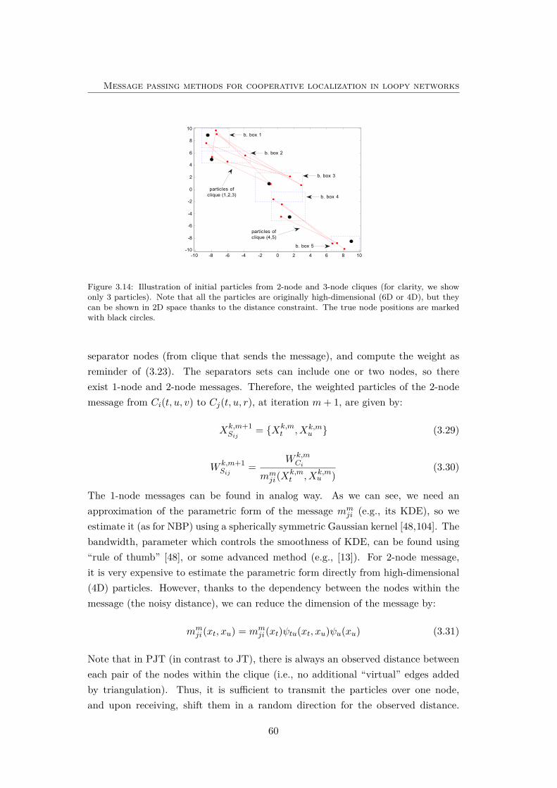
Message passing methods for cooperative localization in loopy networks
-10 -8 -6 -4 -2 0 2 4 6 8 10-10
-8
-6
-4
-2
0
2
4
6
8
10
particles of clique (1,2,3)
particles of clique (4,5)
b. box 1
b. box 2
b. box 3
b. box 4
b. box 5
Figure 3.14: Illustration of initial particles from 2-node and 3-node cliques (for clarity, we showonly 3 particles). Note that all the particles are originally high-dimensional (6D or 4D), but theycan be shown in 2D space thanks to the distance constraint. The true node positions are markedwith black circles.
separator nodes (from clique that sends the message), and compute the weight asreminder of (3.23). The separators sets can include one or two nodes, so thereexist 1-node and 2-node messages. Therefore, the weighted particles of the 2-nodemessage from Ci(t, u, v) to Cj(t, u, r), at iteration m+ 1, are given by:
Xk,m+1Sij
= {Xk,mt , Xk,m
u } (3.29)
W k,m+1Sij
=W k,mCi
mmji(X
k,mt , Xk,m
u )(3.30)
The 1-node messages can be found in analog way. As we can see, we need anapproximation of the parametric form of the message mm
ji (e.g., its KDE), so weestimate it (as for NBP) using a spherically symmetric Gaussian kernel [48,104]. Thebandwidth, parameter which controls the smoothness of KDE, can be found using“rule of thumb” [48], or some advanced method (e.g., [13]). For 2-node message,it is very expensive to estimate the parametric form directly from high-dimensional(4D) particles. However, thanks to the dependency between the nodes within themessage (the noisy distance), we can reduce the dimension of the message by:
mmji(xt, xu) = mm
ji(xt)ψtu(xt, xu)ψu(xu) (3.31)
Note that in PJT (in contrast to JT), there is always an observed distance betweeneach pair of the nodes within the clique (i.e., no additional “virtual” edges addedby triangulation). Thus, it is sufficient to transmit the particles over one node,and upon receiving, shift them in a random direction for the observed distance.
60
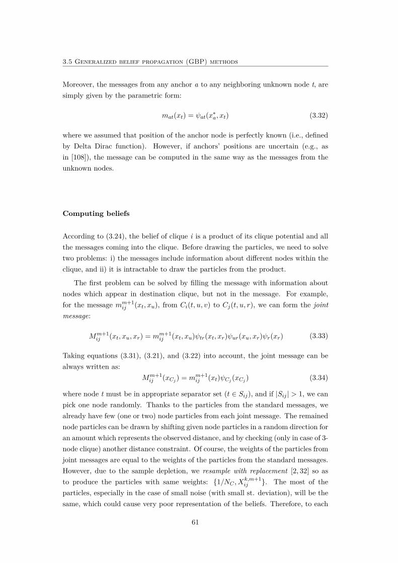
3.5 Generalized belief propagation (GBP) methods
Moreover, the messages from any anchor a to any neighboring unknown node t, aresimply given by the parametric form:
mat(xt) = ψat(x∗a, xt) (3.32)
where we assumed that position of the anchor node is perfectly known (i.e., definedby Delta Dirac function). However, if anchors’ positions are uncertain (e.g., asin [108]), the message can be computed in the same way as the messages from theunknown nodes.
Computing beliefs
According to (3.24), the belief of clique i is a product of its clique potential and allthe messages coming into the clique. Before drawing the particles, we need to solvetwo problems: i) the messages include information about different nodes within theclique, and ii) it is intractable to draw the particles from the product.
The first problem can be solved by filling the message with information aboutnodes which appear in destination clique, but not in the message. For example,for the message mm+1
ij (xt, xu), from Ci(t, u, v) to Cj(t, u, r), we can form the jointmessage:
Mm+1ij (xt, xu, xr) = mm+1
ij (xt, xu)ψtr(xt, xr)ψur(xu, xr)ψr(xr) (3.33)
Taking equations (3.31), (3.21), and (3.22) into account, the joint message can bealways written as:
Mm+1ij (xCj ) = mm+1
ij (xt)ψCj (xCj ) (3.34)
where node t must be in appropriate separator set (t ∈ Sij), and if |Sij | > 1, we canpick one node randomly. Thanks to the particles from the standard messages, wealready have few (one or two) node particles from each joint message. The remainednode particles can be drawn by shifting given node particles in a random direction foran amount which represents the observed distance, and by checking (only in case of 3-node clique) another distance constraint. Of course, the weights of the particles fromjoint messages are equal to the weights of the particles from the standard messages.However, due to the sample depletion, we resample with replacement [2, 32] so asto produce the particles with same weights: {1/NC , X
k,m+1ij }. The most of the
particles, especially in the case of small noise (with small st. deviation), will be thesame, which could cause very poor representation of the beliefs. Therefore, to each
61
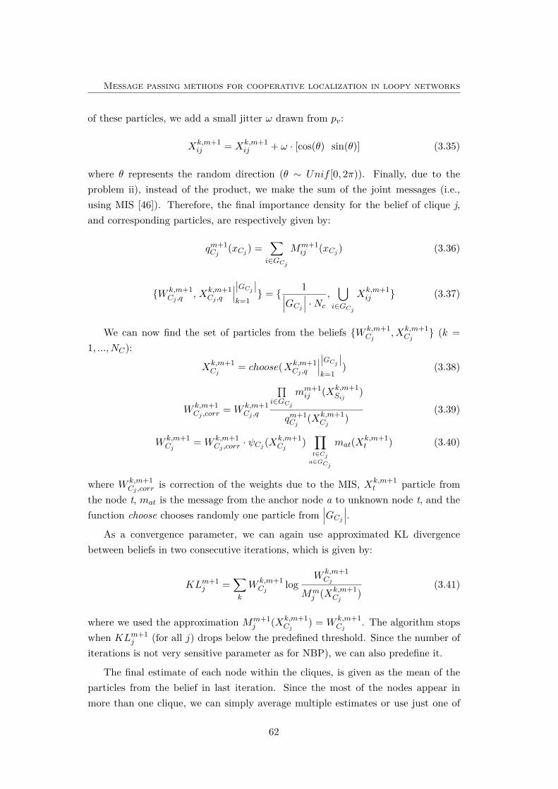
Message passing methods for cooperative localization in loopy networks
of these particles, we add a small jitter ω drawn from pv:
Xk,m+1ij = Xk,m+1
ij + ω · [cos(θ) sin(θ)] (3.35)
where θ represents the random direction (θ ∼ Unif [0, 2π)). Finally, due to theproblem ii), instead of the product, we make the sum of the joint messages (i.e.,using MIS [46]). Therefore, the final importance density for the belief of clique j,and corresponding particles, are respectively given by:
qm+1Cj
(xCj ) =∑i∈GCj
Mm+1ij (xCj ) (3.36)
{W k,m+1Cj ,q
, Xk,m+1Cj ,q
∣∣∣∣∣GCj ∣∣k=1
} = { 1∣∣∣GCj ∣∣∣ ·Nc
,⋃
i∈GCj
Xk,m+1ij } (3.37)
We can now find the set of particles from the beliefs {W k,m+1Cj
, Xk,m+1Cj
} (k =1, ..., NC):
Xk,m+1Cj
= choose(Xk,m+1Cj ,q
∣∣∣∣∣GCj ∣∣k=1
) (3.38)
W k,m+1Cj ,corr
= W k,m+1Cj ,q
∏i∈GCj
mm+1ij (Xk,m+1
Sij)
qm+1Cj
(Xk,m+1Cj
)(3.39)
W k,m+1Cj
= W k,m+1Cj ,corr
· ψCj (Xk,m+1Cj
)∏t∈Cja∈GCj
mat(Xk,m+1t ) (3.40)
where W k,m+1Cj ,corr
is correction of the weights due to the MIS, Xk,m+1t particle from
the node t, mat is the message from the anchor node a to unknown node t, and thefunction choose chooses randomly one particle from
∣∣∣GCj ∣∣∣.As a convergence parameter, we can again use approximated KL divergence
between beliefs in two consecutive iterations, which is given by:
KLm+1j =
∑k
W k,m+1Cj
logW k,m+1Cj
Mmj (Xk,m+1
Cj)
(3.41)
where we used the approximation Mm+1j (Xk,m+1
Cj) = W k,m+1
Cj. The algorithm stops
when KLm+1j (for all j) drops below the predefined threshold. Since the number of
iterations is not very sensitive parameter as for NBP), we can also predefine it.
The final estimate of each node within the cliques, is given as the mean of theparticles from the belief in last iteration. Since the most of the nodes appear inmore than one clique, we can simply average multiple estimates or use just one of
62
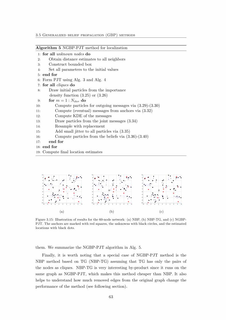
3.5 Generalized belief propagation (GBP) methods
Algorithm 5 NGBP-PJT method for localization1: for all unknown nodes do2: Obtain distance estimates to all neighbors3: Construct bounded box4: Set all parameters to the initial values5: end for6: Form PJT using Alg. 3 and Alg. 47: for all cliques do8: Draw initial particles from the importance
density function (3.25) or (3.26)9: for m = 1 : Niter do
10: Compute particles for outgoing messages via (3.29)-(3.30)11: Compute (eventual) messages from anchors via (3.32)12: Compute KDE of the messages13: Draw particles from the joint messages (3.34)14: Resample with replacement15: Add small jitter to all particles via (3.35)16: Compute particles from the beliefs via (3.36)-(3.40)17: end for18: end for19: Compute final location estimates
-10 -8 -6 -4 -2 0 2 4 6 8 10-10
-8
-6
-4
-2
0
2
4
6
8
10
(a)
-10 -8 -6 -4 -2 0 2 4 6 8 10-10
-8
-6
-4
-2
0
2
4
6
8
10
(b)
-10 -8 -6 -4 -2 0 2 4 6 8 10-10
-8
-6
-4
-2
0
2
4
6
8
10
(c)
Figure 3.15: Illustration of results for the 60-node network: (a) NBP, (b) NBP-TG, and (c) NGBP-PJT. The anchors are marked with red squares, the unknowns with black circles, and the estimatedlocations with black dots.
them. We summarize the NGBP-PJT algorithm in Alg. 5.
Finally, it is worth noting that a special case of NGBP-PJT method is theNBP method based on TG (NBP-TG) assuming that TG has only the pairs ofthe nodes as cliques. NBP-TG is very interesting by-product since it runs on thesame graph as NGBP-PJT, which makes this method cheaper than NBP. It alsohelps to understand how much removed edges from the original graph change theperformance of the method (see following section).
63
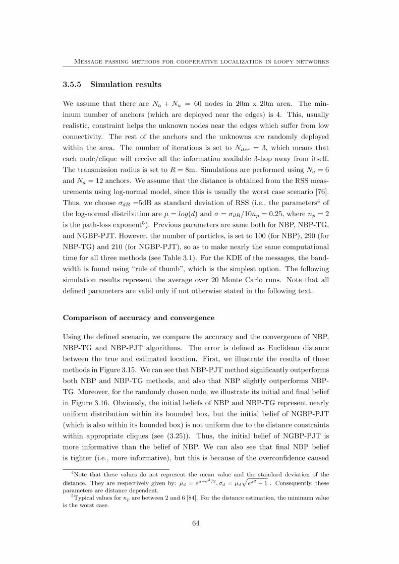
Message passing methods for cooperative localization in loopy networks
3.5.5 Simulation results
We assume that there are Na + Nu = 60 nodes in 20m x 20m area. The min-imum number of anchors (which are deployed near the edges) is 4. This, usuallyrealistic, constraint helps the unknown nodes near the edges which suffer from lowconnectivity. The rest of the anchors and the unknowns are randomly deployedwithin the area. The number of iterations is set to Niter = 3, which means thateach node/clique will receive all the information available 3-hop away from itself.The transmission radius is set to R = 8m. Simulations are performed using Na = 6and Na = 12 anchors. We assume that the distance is obtained from the RSS meas-urements using log-normal model, since this is usually the worst case scenario [76].Thus, we choose σdB =5dB as standard deviation of RSS (i.e., the parameters4 ofthe log-normal distribution are µ = log(d) and σ = σdB/10np = 0.25, where np = 2is the path-loss exponent5). Previous parameters are same both for NBP, NBP-TG,and NGBP-PJT. However, the number of particles, is set to 100 (for NBP), 290 (forNBP-TG) and 210 (for NGBP-PJT), so as to make nearly the same computationaltime for all three methods (see Table 3.1). For the KDE of the messages, the band-width is found using “rule of thumb”, which is the simplest option. The followingsimulation results represent the average over 20 Monte Carlo runs. Note that alldefined parameters are valid only if not otherwise stated in the following text.
Comparison of accuracy and convergence
Using the defined scenario, we compare the accuracy and the convergence of NBP,NBP-TG and NBP-PJT algorithms. The error is defined as Euclidean distancebetween the true and estimated location. First, we illustrate the results of thesemethods in Figure 3.15. We can see that NBP-PJT method significantly outperformsboth NBP and NBP-TG methods, and also that NBP slightly outperforms NBP-TG. Moreover, for the randomly chosen node, we illustrate its initial and final beliefin Figure 3.16. Obviously, the initial beliefs of NBP and NBP-TG represent nearlyuniform distribution within its bounded box, but the initial belief of NGBP-PJT(which is also within its bounded box) is not uniform due to the distance constraintswithin appropriate cliques (see (3.25)). Thus, the initial belief of NGBP-PJT ismore informative than the belief of NBP. We can also see that final NBP beliefis tighter (i.e., more informative), but this is because of the overconfidence caused
4Note that these values do not represent the mean value and the standard deviation of thedistance. They are respectively given by: µd = eµ+σ2/2, σd = µd
√eσ2 − 1 . Consequently, these
parameters are distance dependent.5Typical values for np are between 2 and 6 [84]. For the distance estimation, the minimum value
is the worst case.
64
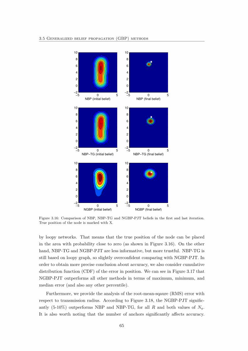
3.5 Generalized belief propagation (GBP) methods
NBP (initial belief)
−5 0 5−2
0
2
4
6
8
10
NBP (final belief)
−5 0 5−2
0
2
4
6
8
10
NBP−TG (initial belief)
−5 0 5−2
0
2
4
6
8
10
NBP−TG (final belief)
−5 0 5−2
0
2
4
6
8
10
NGBP (initial belief)
−5 0 5−2
0
2
4
6
8
10
NGBP (final belief)
−5 0 5−2
0
2
4
6
8
10
Figure 3.16: Comparison of NBP, NBP-TG and NGBP-PJT beliefs in the first and last iteration.True position of the node is marked with X.
by loopy networks. That means that the true position of the node can be placedin the area with probability close to zero (as shown in Figure 3.16). On the otherhand, NBP-TG and NGBP-PJT are less informative, but more trustful. NBP-TG isstill based on loopy graph, so slightly overconfident comparing with NGBP-PJT. Inorder to obtain more precise conclusion about accuracy, we also consider cumulativedistribution function (CDF) of the error in position. We can see in Figure 3.17 thatNGBP-PJT outperforms all other methods in terms of maximum, minimum, andmedian error (and also any other percentile).
Furthermore, we provide the analysis of the root-mean-sqaure (RMS) error withrespect to transmission radius. According to Figure 3.18, the NGBP-PJT signific-antly (5-10%) outperforms NBP and NBP-TG, for all R and both values of Na.It is also worth noting that the number of anchors significantly affects accuracy.
65
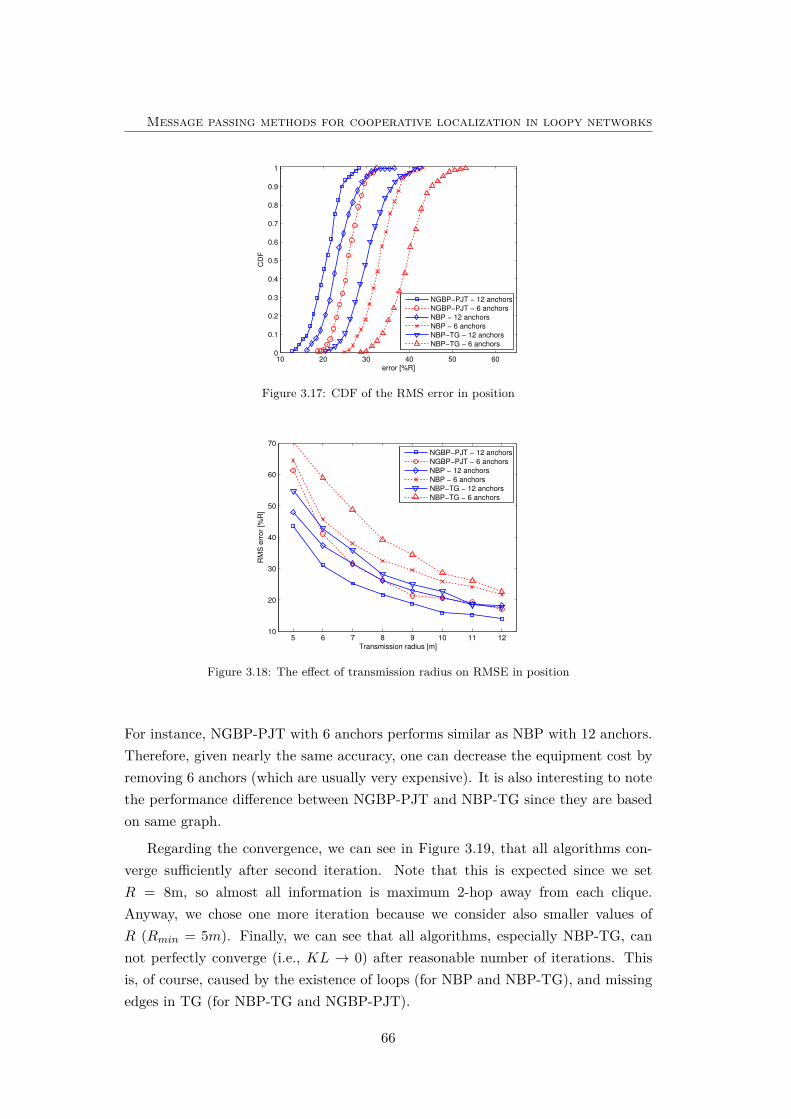
Message passing methods for cooperative localization in loopy networks
10 20 30 40 50 600
0.1
0.2
0.3
0.4
0.5
0.6
0.7
0.8
0.9
1
error [%R]
CD
F
NGBP−PJT − 12 anchors
NGBP−PJT − 6 anchors
NBP − 12 anchors
NBP − 6 anchors
NBP−TG − 12 anchors
NBP−TG − 6 anchors
Figure 3.17: CDF of the RMS error in position
5 6 7 8 9 10 11 1210
20
30
40
50
60
70
Transmission radius [m]
RM
S e
rror
[%R
]
NGBP−PJT − 12 anchors
NGBP−PJT − 6 anchors
NBP − 12 anchors
NBP − 6 anchors
NBP−TG − 12 anchors
NBP−TG − 6 anchors
Figure 3.18: The effect of transmission radius on RMSE in position
For instance, NGBP-PJT with 6 anchors performs similar as NBP with 12 anchors.Therefore, given nearly the same accuracy, one can decrease the equipment cost byremoving 6 anchors (which are usually very expensive). It is also interesting to notethe performance difference between NGBP-PJT and NBP-TG since they are basedon same graph.
Regarding the convergence, we can see in Figure 3.19, that all algorithms con-verge sufficiently after second iteration. Note that this is expected since we setR = 8m, so almost all information is maximum 2-hop away from each clique.Anyway, we chose one more iteration because we consider also smaller values ofR (Rmin = 5m). Finally, we can see that all algorithms, especially NBP-TG, cannot perfectly converge (i.e., KL → 0) after reasonable number of iterations. Thisis, of course, caused by the existence of loops (for NBP and NBP-TG), and missingedges in TG (for NBP-TG and NGBP-PJT).
66
3.5 Generalized belief propagation (GBP) methods
0 2 4 6 8 100.2
0.3
0.4
0.5
0.6
0.7
0.8
0.9
Iteration number
KL d
iverg
ence
NGBP−PJT − 12 anchors
NGBP−PJT − 6 anchors
NBP − 12 anchors
NBP − 6 anchors
NBP−TG − 12 anchors
NBP−TG − 6 anchors
Figure 3.19: Comparison of KL divergence in each iteration
Table 3.1: Comparison of the computational cost (measured in MFlops)
R NBP NBP-TG NGBP-PJT PJT
5m 0.56 0.56 0.56 0.0078m 0.71 0.59 0.67 0.01112m 0.82 0.62 0.73 0.013
Comparison of computational and communication cost
As we already mentioned, we set the same computational cost for R = 5m bychoosing appropriate number of particles for all three methods. It was not possibleto set the same cost for all methods (R > 5m) because the cost is more sensitive toR in case of NBP. On other hand, NGBP-PJT and NBP-TG costs are less sensitiveto R due to the nearly same number of edges with respect to R, in formed TG. Weprovide the average cost per node for different values of R in Table 3.1. We can seethat the cost of NGBP-PJT is the same or less for all considered values of R. Wecan also see that complexity of the PJT formation is negligible comparing with fullalgorithms.
Regarding communication cost, which is very important for the battery life of thewireless devices, we count elementary messages (i.e, scalar values). We will considerthe effect of transmission radius and number of unknowns, since their variationsobviously affect the cost. First, we analyse the cost of PJT formation (Alg. 1 andAlg. 2). As we can see in Figure 3.20, it is a linear function of transmission radius,and a quadratic function of number of unknowns. Second, we analyse the cost of allconsidered algorithms w.r.t. R for 2 different number of unknowns. According toFigure 3.21, we can conclude the following:
67
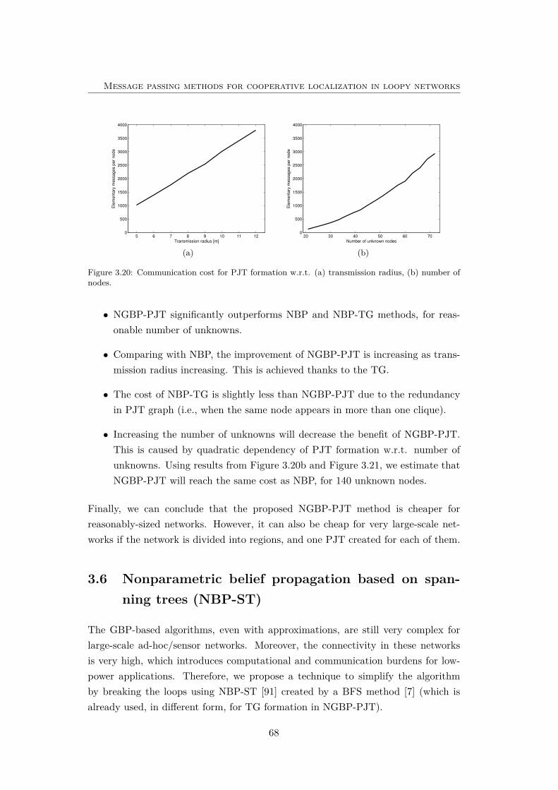
Message passing methods for cooperative localization in loopy networks
5 6 7 8 9 10 11 120
500
1000
1500
2000
2500
3000
3500
4000
Transmission radius [m]
Ele
me
nta
ry m
essa
ge
s p
er
no
de
(a)
20 30 40 50 60 700
500
1000
1500
2000
2500
3000
3500
4000
Number of unknown nodes
Ele
me
nta
ry m
essa
ge
s p
er
no
de
(b)
Figure 3.20: Communication cost for PJT formation w.r.t. (a) transmission radius, (b) number ofnodes.
• NGBP-PJT significantly outperforms NBP and NBP-TG methods, for reas-onable number of unknowns.
• Comparing with NBP, the improvement of NGBP-PJT is increasing as trans-mission radius increasing. This is achieved thanks to the TG.
• The cost of NBP-TG is slightly less than NGBP-PJT due to the redundancyin PJT graph (i.e., when the same node appears in more than one clique).
• Increasing the number of unknowns will decrease the benefit of NGBP-PJT.This is caused by quadratic dependency of PJT formation w.r.t. number ofunknowns. Using results from Figure 3.20b and Figure 3.21, we estimate thatNGBP-PJT will reach the same cost as NBP, for 140 unknown nodes.
Finally, we can conclude that the proposed NGBP-PJT method is cheaper forreasonably-sized networks. However, it can also be cheap for very large-scale net-works if the network is divided into regions, and one PJT created for each of them.
3.6 Nonparametric belief propagation based on span-ning trees (NBP-ST)
The GBP-based algorithms, even with approximations, are still very complex forlarge-scale ad-hoc/sensor networks. Moreover, the connectivity in these networksis very high, which introduces computational and communication burdens for low-power applications. Therefore, we propose a technique to simplify the algorithmby breaking the loops using NBP-ST [91] created by a BFS method [7] (which isalready used, in different form, for TG formation in NGBP-PJT).
68
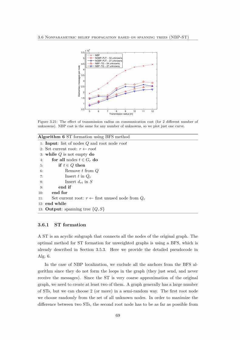
3.6 Nonparametric belief propagation based on spanning trees (NBP-ST)
5 6 7 8 9 10 11 120.5
1
1.5
2
2.5
3
3.5
4
4.5
5
5.5x 10
4
Transmission radius [m]
Ele
menta
ry m
essages p
er
node
NBP
NGBP−PJT − 54 unknowns
NGBP−PJT − 27 unknowns
NBP−TG − 54 unknowns
NBP−TG − 27 unknowns
Figure 3.21: The effect of transmission radius on communication cost (for 2 different number ofunknowns). NBP cost is the same for any number of unknowns, so we plot just one curve.
Algorithm 6 ST formation using BFS method1: Input: list of nodes Q and root node root2: Set current root: r ← root3: while Q is not empty do4: for all nodes t ∈ Gr do5: if t ∈ Q then6: Remove t from Q7: Insert t in Qr8: Insert drt in S9: end if
10: end for11: Set current root: r ← first unused node from Qr12: end while13: Output: spanning tree {Q,S}
3.6.1 ST formation
A ST is an acyclic subgraph that connects all the nodes of the original graph. Theoptimal method for ST formation for unweighted graphs is using a BFS, which isalready described in Section 3.5.3. Here we provide the detailed pseudocode inAlg. 6.
In the case of NBP localization, we exclude all the anchors from the BFS al-gorithm since they do not form the loops in the graph (they just send, and neverreceive the messages). Since the ST is very coarse approximation of the originalgraph, we need to create at least two of them. A graph generally has a large numberof STs, but we can choose 2 (or more) in a semi-random way. The first root nodewe choose randomly from the set of all unknown nodes. In order to maximize thedifference between two STs, the second root node has to be as far as possible from
69
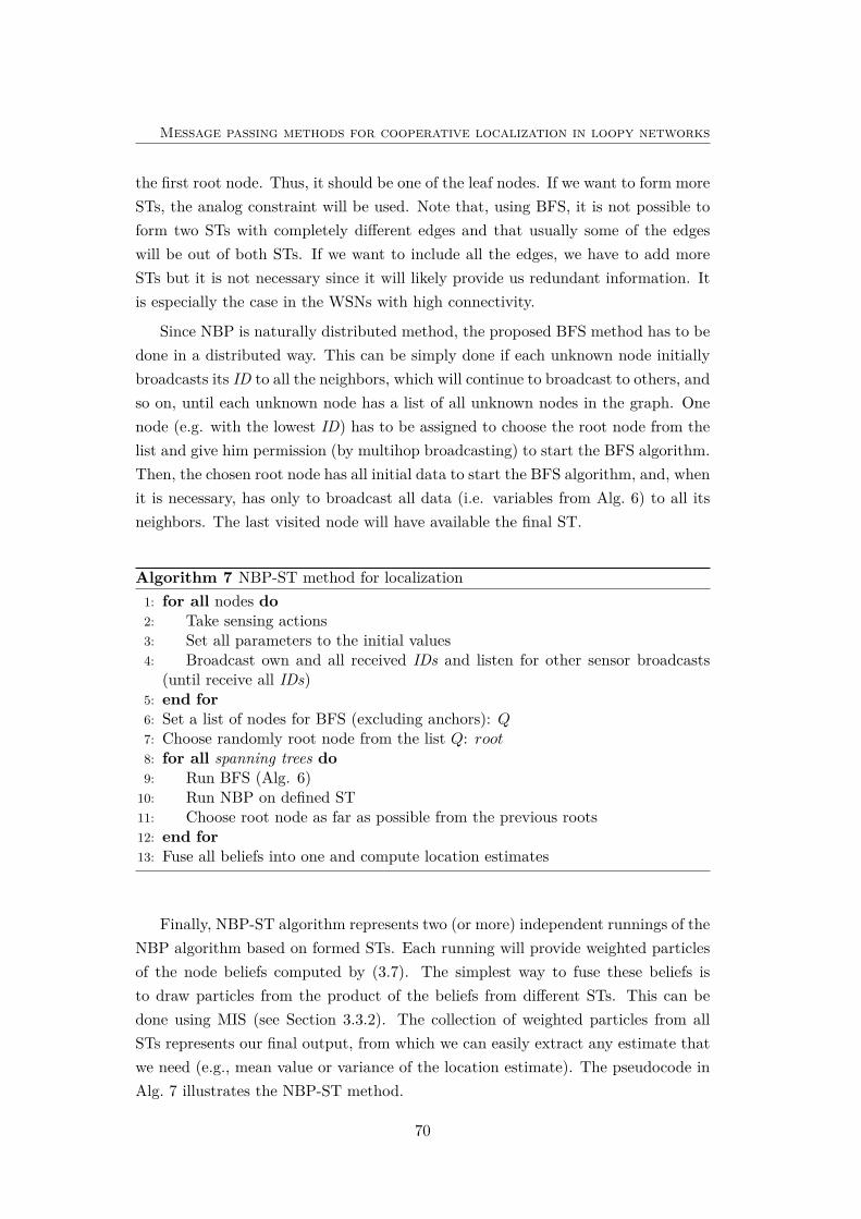
Message passing methods for cooperative localization in loopy networks
the first root node. Thus, it should be one of the leaf nodes. If we want to form moreSTs, the analog constraint will be used. Note that, using BFS, it is not possible toform two STs with completely different edges and that usually some of the edgeswill be out of both STs. If we want to include all the edges, we have to add moreSTs but it is not necessary since it will likely provide us redundant information. Itis especially the case in the WSNs with high connectivity.
Since NBP is naturally distributed method, the proposed BFS method has to bedone in a distributed way. This can be simply done if each unknown node initiallybroadcasts its ID to all the neighbors, which will continue to broadcast to others, andso on, until each unknown node has a list of all unknown nodes in the graph. Onenode (e.g. with the lowest ID) has to be assigned to choose the root node from thelist and give him permission (by multihop broadcasting) to start the BFS algorithm.Then, the chosen root node has all initial data to start the BFS algorithm, and, whenit is necessary, has only to broadcast all data (i.e. variables from Alg. 6) to all itsneighbors. The last visited node will have available the final ST.
Algorithm 7 NBP-ST method for localization1: for all nodes do2: Take sensing actions3: Set all parameters to the initial values4: Broadcast own and all received IDs and listen for other sensor broadcasts
(until receive all IDs)5: end for6: Set a list of nodes for BFS (excluding anchors): Q7: Choose randomly root node from the list Q: root8: for all spanning trees do9: Run BFS (Alg. 6)
10: Run NBP on defined ST11: Choose root node as far as possible from the previous roots12: end for13: Fuse all beliefs into one and compute location estimates
Finally, NBP-ST algorithm represents two (or more) independent runnings of theNBP algorithm based on formed STs. Each running will provide weighted particlesof the node beliefs computed by (3.7). The simplest way to fuse these beliefs isto draw particles from the product of the beliefs from different STs. This can bedone using MIS (see Section 3.3.2). The collection of weighted particles from allSTs represents our final output, from which we can easily extract any estimate thatwe need (e.g., mean value or variance of the location estimate). The pseudocode inAlg. 7 illustrates the NBP-ST method.
70
3.6 Nonparametric belief propagation based on spanning trees (NBP-ST)
-10 -8 -6 -4 -2 0 2 4 6 8 10-10
-8
-6
-4
-2
0
2
4
6
8
10
1
2
3
4
5
6
7
8 910
11
12
13
1415
16
17
18
19
20
2122
23
2425
26
27
28
29
30
3132
33
3435
36
37
38
3940
41
42
43
44
45
46
47
48
49
50
51
52
53
54
55
56
5758
59
60
61
62
6364
65
66
67
68
6970
71
72
73
74
7576
7778
79
80
81
82
83
84
85
86
87
88
8990
91
92
93
9495
96
97
98
99100
101
102
103
104105
106
107
108
109
110
(a)
-10 -8 -6 -4 -2 0 2 4 6 8 10-10
-8
-6
-4
-2
0
2
4
6
8
10
1
2
3
4
5
6
7
8 910
11
12
13
1415
16
17
18
19
20
2122
23
2425
26
27
28
29
30
3132
33
3435
36
37
38
3940
41
42
43
44
45
46
47
48
49
50
51
52
53
54
55
56
5758
59
60
61
62
6364
65
66
67
68
6970
71
72
73
74
7576
7778
79
80
81
82
83
84
85
86
87
88
8990
91
92
93
9495
96
97
98
99100
101
102
103
104105
106
107
108
109
110
(b)
-10 -8 -6 -4 -2 0 2 4 6 8 10-10
-8
-6
-4
-2
0
2
4
6
8
10
1
2
3
4
5
6
7
8 910
11
12
13
1415
16
17
18
19
20
2122
23
2425
26
27
28
29
30
3132
33
3435
36
37
38
3940
41
42
43
44
45
46
47
48
49
50
51
52
53
54
55
56
5758
59
60
61
62
6364
65
66
67
68
6970
71
72
73
74
7576
7778
79
80
81
82
83
84
85
86
87
88
8990
91
92
93
9495
96
97
98
99100
101
102
103
104105
106
107
108
109
110
(c)
Figure 3.22: (a) Original network with 100 unknown nodes (black dots) and 10 anchors (red as-terisks) for R = 6m, and (b), (c) Two corresponding STs. The roots are node 103 and node 71,respectively.
3.6.2 Simulation results
To illustrate the performance of this method, we conducted several simulations.We assume that there are 100 unknown and 10 anchor nodes randomly deployedin 20m x 20m area. Since the unknown nodes near the edges of the deploymentarea suffer from low connectivity, we make an exception for four anchors, which arerandomly deployed within four square-shaped areas of 4m x 4m near the edges. Thestandard deviation of the Gaussian noise on the distance estimate is set to σ = 0.3mand the number of iteration is set to Niter = 3. All simulations are done for N = 50and N = 100 particles with respect to the transmission radius (R = 4m - 10m).Each point in the simulations represents the average over 20 Monte Carlo trials.
Using the defined scenario, we compared NBP and NBP-ST algorithms. ForNBP-ST, we used 2 STs. The original network and 2 STs created by BFS areillustrated in Figure 3.22. Regarding accuracy and coverage in Figure 3.23, NBP-ST performs better than NBP for R > 7m, approximately. Obviously, for thesevalues of R there is a large number of loops in the network which decreases theperformance of the NBP method. For lower values of R, we could expect that NBP-ST performs with higher (or same) accuracy, but we cannot forget that, by usingonly 2 STs, we do not include all information (i.e., removed edges) that we have.Thus, the NBP outperforms NBP-ST in this case.
Regarding the computational/communication cost (Figure 3.24), NBP-ST per-forms better than NBP for R > 8m and R > 9m, respectively. In order to explainthis result, we should recall two main things we have taken into account: i) remov-ing the edges in order to form the STs, and ii) running NBP two times in theseSTs. The former decreases the computational/communication cost, but the latterone increases it. Therefore, in the low-connected networks the second operation pre-dominates, but in the highly-connected networks the first one predominates. The
71
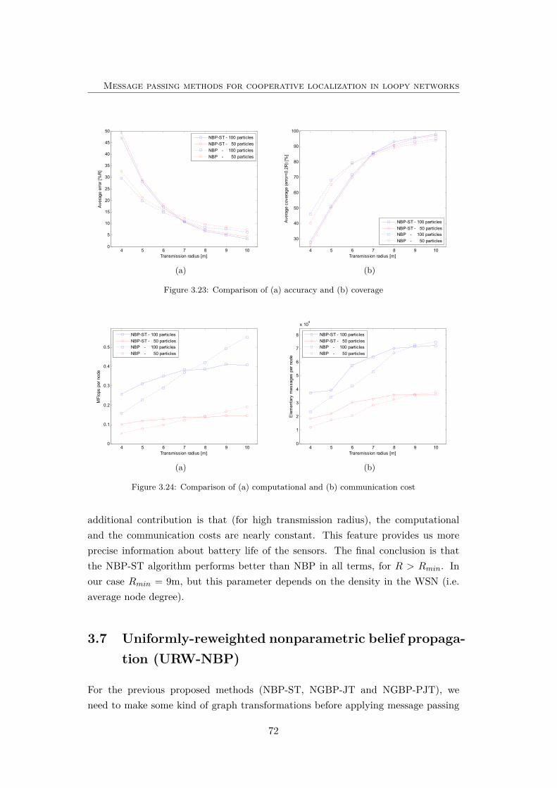
Message passing methods for cooperative localization in loopy networks
4 5 6 7 8 9 100
5
10
15
20
25
30
35
40
45
50
Transmission radius [m]
Ave
rage
erro
r [%
R]
NBP-ST - 100 particlesNBP-ST - 50 particlesNBP - 100 particlesNBP - 50 particles
(a)
4 5 6 7 8 9 10
30
40
50
60
70
80
90
100
Transmission radius [m]
Ave
rage
cov
erag
e (e
rror<
0.2R
) [%
]
NBP-ST - 100 particlesNBP-ST - 50 particlesNBP - 100 particlesNBP - 50 particles
(b)
Figure 3.23: Comparison of (a) accuracy and (b) coverage
4 5 6 7 8 9 100
0.1
0.2
0.3
0.4
0.5
Transmission radius [m]
MFl
ops
per n
ode
NBP-ST - 100 particlesNBP-ST - 50 particlesNBP - 100 particlesNBP - 50 particles
(a)
4 5 6 7 8 9 100
1
2
3
4
5
6
7
8
x 104
Transmission radius [m]
Ele
men
tary
mes
sage
s pe
r nod
e
NBP-ST - 100 particlesNBP-ST - 50 particlesNBP - 100 particlesNBP - 50 particles
(b)
Figure 3.24: Comparison of (a) computational and (b) communication cost
additional contribution is that (for high transmission radius), the computationaland the communication costs are nearly constant. This feature provides us moreprecise information about battery life of the sensors. The final conclusion is thatthe NBP-ST algorithm performs better than NBP in all terms, for R > Rmin. Inour case Rmin = 9m, but this parameter depends on the density in the WSN (i.e.average node degree).
3.7 Uniformly-reweighted nonparametric belief propaga-tion (URW-NBP)
For the previous proposed methods (NBP-ST, NGBP-JT and NGBP-PJT), weneed to make some kind of graph transformations before applying message passing
72
3.7 Uniformly-reweighted nonparametric belief propagation (URW-NBP)
method. This usually reduces the robustness of the whole algorithm, since the fail-ure of just one node can make significant effect on the localization performance.In addition, it is necessary to synchronize whole network, which is sometimes notpossible. Since standard NBP is robust to node failures, and capable to run inasynchronous networks [24], our goal is to find an improved method with the samefeatures. Therefore, we propose a method based on tree-reweighted BP (TRW-BP)proposed in [110].
In the standard TRW-BP algorithm the belief at a node t is proportional tothe product of the local evidence at that node ψt(xt), and all reweighted messagescoming into node t:
Mt(xt) ∝ ψt(xt)∏u∈Gt
mut(xt)ρut , (3.42)
where xt is a state of node t, ρtu = ρut is the appearance probability of the edge(t, u), and Gt denotes the neighbors of node t. The messages are determined by themessage update rule:
mut(xt) ∝ˆψu(xu)ψtu(xt, xu)1/ρtu
∏k∈Gu\t
mku(xu)ρkumtu(xu)1−ρtu dxu, (3.43)
where ψtu(xt, xu) is the pairwise potential between nodes t and u. On the right-handside, there is a product over all reweighted messages going into node u except forthe one coming from node t. The update-rule (3.43) is carried out over the network.Upon convergence, the beliefs are computed through (3.42). As in the case of NBP,it is more convenient to compute the beliefs at every iteration i. This leads to anequivalent form of TRW-BP: by replacing (3.42) in (3.43), we find that the beliefequations and message-update rule of TRW-BP are, respectively, given by:
M it (xt) ∝ ψt(xt)
∏u∈Gt
miut(xt)ρut (3.44)
miut(xt) ∝
ˆψut(xt, xu)1/ρut M
i−1u (xu)
mi−1tu (xu)
dxu. (3.45)
We can now apply TRW-BP to the localization problem. In the first iteration ofthis algorithm it is necessary to initialize m1
ut = 1 and M1t = pt (i.e., information
from anchors, if any) for all u, t, and then repeat computation using (3.44) and(3.45) until convergence or a preset number of iterations is attained. In a practicalimplementation, we have to use nonparametric version of TRW-BP (TRW-NBP).Hence, the beliefs and message update equations, (3.44) and (3.45), are performedusing particle-based approximations. Since this approximation is done in the sameway as for NBP, see Section 3.3 (and also [46,88]) for more details.
73
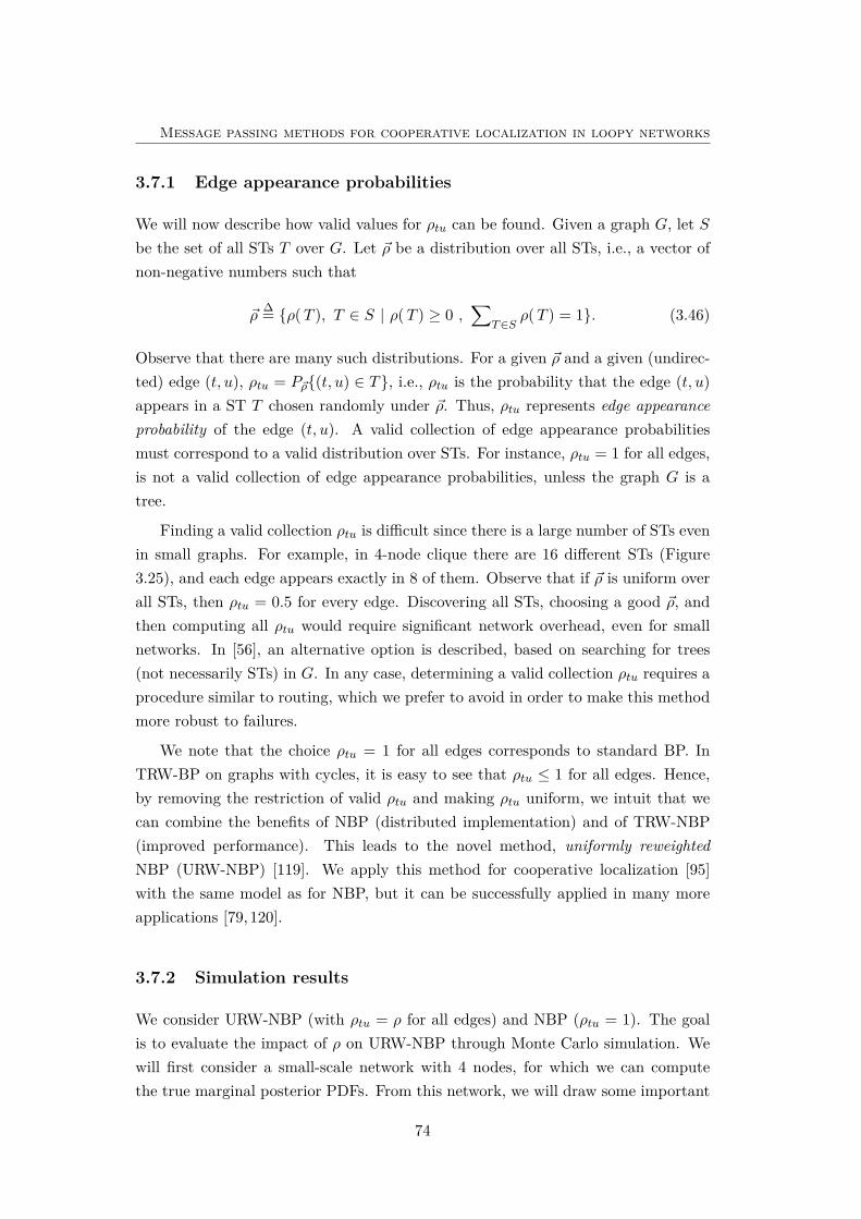
Message passing methods for cooperative localization in loopy networks
3.7.1 Edge appearance probabilities
We will now describe how valid values for ρtu can be found. Given a graph G, let Sbe the set of all STs T over G. Let ~ρ be a distribution over all STs, i.e., a vector ofnon-negative numbers such that
~ρ∆= {ρ(T ), T ∈ S | ρ(T ) ≥ 0 ,
∑T∈S
ρ(T ) = 1}. (3.46)
Observe that there are many such distributions. For a given ~ρ and a given (undirec-ted) edge (t, u), ρtu = P~ρ{(t, u) ∈ T}, i.e., ρtu is the probability that the edge (t, u)appears in a ST T chosen randomly under ~ρ. Thus, ρtu represents edge appearanceprobability of the edge (t, u). A valid collection of edge appearance probabilitiesmust correspond to a valid distribution over STs. For instance, ρtu = 1 for all edges,is not a valid collection of edge appearance probabilities, unless the graph G is atree.
Finding a valid collection ρtu is difficult since there is a large number of STs evenin small graphs. For example, in 4-node clique there are 16 different STs (Figure3.25), and each edge appears exactly in 8 of them. Observe that if ~ρ is uniform overall STs, then ρtu = 0.5 for every edge. Discovering all STs, choosing a good ~ρ, andthen computing all ρtu would require significant network overhead, even for smallnetworks. In [56], an alternative option is described, based on searching for trees(not necessarily STs) in G. In any case, determining a valid collection ρtu requires aprocedure similar to routing, which we prefer to avoid in order to make this methodmore robust to failures.
We note that the choice ρtu = 1 for all edges corresponds to standard BP. InTRW-BP on graphs with cycles, it is easy to see that ρtu ≤ 1 for all edges. Hence,by removing the restriction of valid ρtu and making ρtu uniform, we intuit that wecan combine the benefits of NBP (distributed implementation) and of TRW-NBP(improved performance). This leads to the novel method, uniformly reweightedNBP (URW-NBP) [119]. We apply this method for cooperative localization [95]with the same model as for NBP, but it can be successfully applied in many moreapplications [79,120].
3.7.2 Simulation results
We consider URW-NBP (with ρtu = ρ for all edges) and NBP (ρtu = 1). The goalis to evaluate the impact of ρ on URW-NBP through Monte Carlo simulation. Wewill first consider a small-scale network with 4 nodes, for which we can computethe true marginal posterior PDFs. From this network, we will draw some important
74
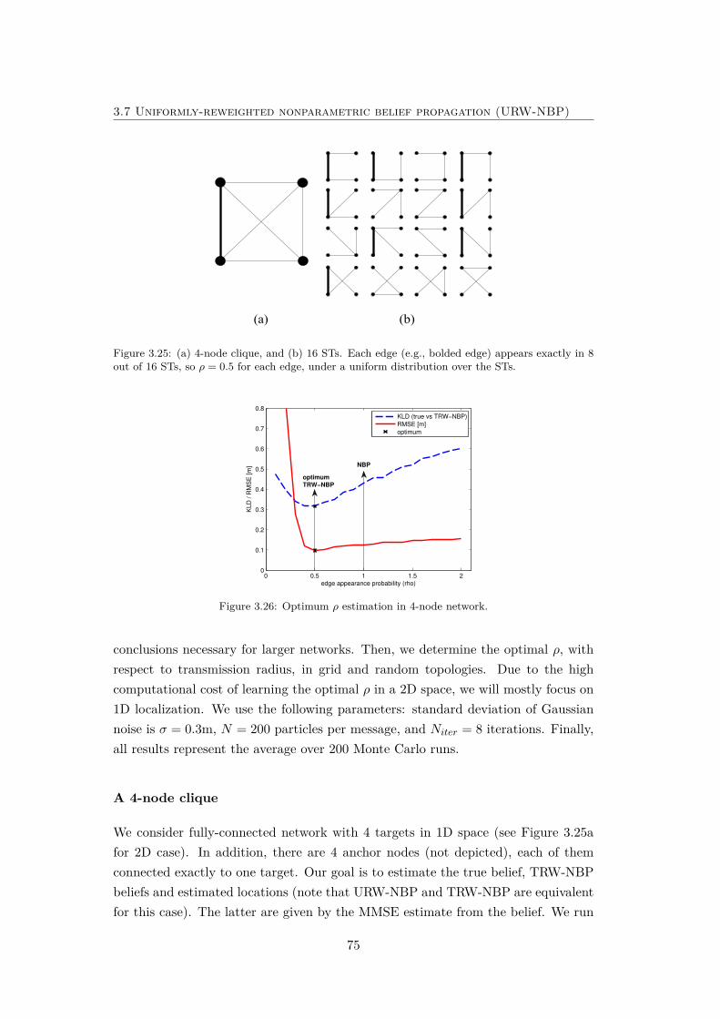
3.7 Uniformly-reweighted nonparametric belief propagation (URW-NBP)
(a) (b)
Figure 3.25: (a) 4-node clique, and (b) 16 STs. Each edge (e.g., bolded edge) appears exactly in 8out of 16 STs, so ρ = 0.5 for each edge, under a uniform distribution over the STs.
0 0.5 1 1.5 20
0.1
0.2
0.3
0.4
0.5
0.6
0.7
0.8
edge appearance probability (rho)
KL
D /
RM
SE
[m
]
KLD (true vs TRW−NBP)
RMSE [m]
optimum
optimumTRW−NBP
NBP
Figure 3.26: Optimum ρ estimation in 4-node network.
conclusions necessary for larger networks. Then, we determine the optimal ρ, withrespect to transmission radius, in grid and random topologies. Due to the highcomputational cost of learning the optimal ρ in a 2D space, we will mostly focus on1D localization. We use the following parameters: standard deviation of Gaussiannoise is σ = 0.3m, N = 200 particles per message, and Niter = 8 iterations. Finally,all results represent the average over 200 Monte Carlo runs.
A 4-node clique
We consider fully-connected network with 4 targets in 1D space (see Figure 3.25afor 2D case). In addition, there are 4 anchor nodes (not depicted), each of themconnected exactly to one target. Our goal is to estimate the true belief, TRW-NBPbeliefs and estimated locations (note that URW-NBP and TRW-NBP are equivalentfor this case). The latter are given by the MMSE estimate from the belief. We run
75
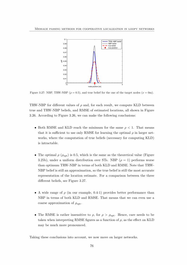
Message passing methods for cooperative localization in loopy networks
−5 0 50
0.01
0.02
0.03
0.04
0.05
0.06
0.07
0.08
0.09
0.1
node position [m]
pd
f
TRW−NBP belief
NBP belief
true belief
true position
Figure 3.27: NBP, TRW-NBP (ρ = 0.5), and true belief for the one of the target nodes (x = 0m).
TRW-NBP for different values of ρ and, for each result, we compute KLD betweentrue and TRW-NBP beliefs, and RMSE of estimated locations, all shown in Figure3.26. According to Figure 3.26, we can make the following conclusions:
• Both RMSE and KLD reach the minimum for the same ρ < 1. That meansthat it is sufficient to use only RMSE for learning the optimal ρ in larger net-works, where the computation of true beliefs (necessary for computing KLD)is intractable.
• The optimal ρ (ρopt) is 0.5, which is the same as the theoretical value (Figure3.25b), under a uniform distribution over STs. NBP (ρ = 1) performs worsethan optimum TRW-NBP in terms of both KLD and RMSE. Note that TRW-NBP belief is still an approximation, so the true belief is still the most accuraterepresentation of the location estimate. For a comparison between the threedifferent beliefs, see Figure 3.27.
• A wide range of ρ (in our example, 0.4-1) provides better performance thanNBP in terms of both KLD and RMSE. That means that we can even use acoarse approximation of ρopt.
• The RMSE is rather insensitive to ρ, for ρ > ρopt. Hence, care needs to betaken when interpreting RMSE figures as a function of ρ, as the effect on KLDmay be much more pronounced.
Taking these conclusions into account, we now move on larger networks.
76
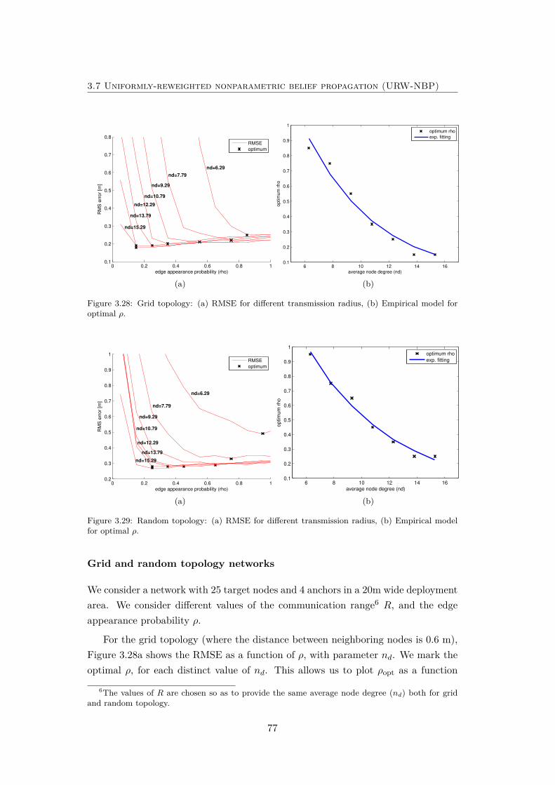
3.7 Uniformly-reweighted nonparametric belief propagation (URW-NBP)
0 0.2 0.4 0.6 0.8 10.1
0.2
0.3
0.4
0.5
0.6
0.7
0.8
edge appearance probability (rho)
RM
S e
rro
r [m
]
RMSE
optimum
nd=7.79
nd=12.29
nd=13.79
nd=15.29
nd=9.29
nd=10.79
nd=6.29
(a)
6 8 10 12 14 160.1
0.2
0.3
0.4
0.5
0.6
0.7
0.8
0.9
1
average node degree (nd)optim
um
rho
optimum rho
exp. fitting
(b)
Figure 3.28: Grid topology: (a) RMSE for different transmission radius, (b) Empirical model foroptimal ρ.
0 0.2 0.4 0.6 0.8 10.2
0.3
0.4
0.5
0.6
0.7
0.8
0.9
1
edge appearance probability (rho)
RM
S e
rro
r [m
]
RMSE
optimum
nd=6.29
nd=9.29
nd=12.29
nd=13.79
nd=15.29
nd=10.79
nd=7.79
(a)
6 8 10 12 14 160.1
0.2
0.3
0.4
0.5
0.6
0.7
0.8
0.9
1
average node degree (nd)
optim
um
rho
optimum rho
exp. fitting
(b)
Figure 3.29: Random topology: (a) RMSE for different transmission radius, (b) Empirical modelfor optimal ρ.
Grid and random topology networks
We consider a network with 25 target nodes and 4 anchors in a 20m wide deploymentarea. We consider different values of the communication range6 R, and the edgeappearance probability ρ.
For the grid topology (where the distance between neighboring nodes is 0.6 m),Figure 3.28a shows the RMSE as a function of ρ, with parameter nd. We mark theoptimal ρ, for each distinct value of nd. This allows us to plot ρopt as a function
6The values of R are chosen so as to provide the same average node degree (nd) both for gridand random topology.
77
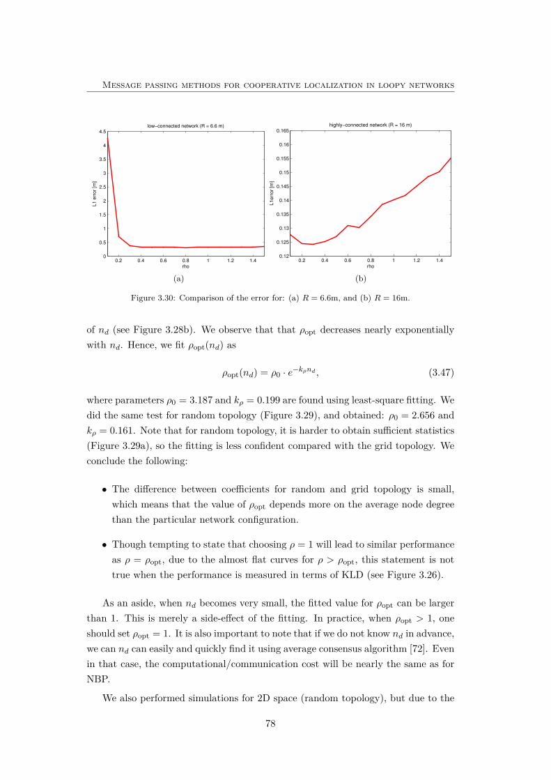
Message passing methods for cooperative localization in loopy networks
0.2 0.4 0.6 0.8 1 1.2 1.40
0.5
1
1.5
2
2.5
3
3.5
4
4.5
rho
L1
err
or
[m]
low−connected network (R = 6.6 m)
(a)
0.2 0.4 0.6 0.8 1 1.2 1.40.12
0.125
0.13
0.135
0.14
0.145
0.15
0.155
0.16
0.165
rhoL
1e
rro
r [m
]
highly−connected network (R = 16 m)
(b)
Figure 3.30: Comparison of the error for: (a) R = 6.6m, and (b) R = 16m.
of nd (see Figure 3.28b). We observe that that ρopt decreases nearly exponentiallywith nd. Hence, we fit ρopt(nd) as
ρopt(nd) = ρ0 · e−kρnd , (3.47)
where parameters ρ0 = 3.187 and kρ = 0.199 are found using least-square fitting. Wedid the same test for random topology (Figure 3.29), and obtained: ρ0 = 2.656 andkρ = 0.161. Note that for random topology, it is harder to obtain sufficient statistics(Figure 3.29a), so the fitting is less confident compared with the grid topology. Weconclude the following:
• The difference between coefficients for random and grid topology is small,which means that the value of ρopt depends more on the average node degreethan the particular network configuration.
• Though tempting to state that choosing ρ = 1 will lead to similar performanceas ρ = ρopt, due to the almost flat curves for ρ > ρopt, this statement is nottrue when the performance is measured in terms of KLD (see Figure 3.26).
As an aside, when nd becomes very small, the fitted value for ρopt can be largerthan 1. This is merely a side-effect of the fitting. In practice, when ρopt > 1, oneshould set ρopt = 1. It is also important to note that if we do not know nd in advance,we can nd can easily and quickly find it using average consensus algorithm [72]. Evenin that case, the computational/communication cost will be nearly the same as forNBP.
We also performed simulations for 2D space (random topology), but due to the
78
3.8 Summary
computational problems, only for 2 representative values of R. In this case, weused N = 500 particles, and Niter = 10 iterations. We observe in Figure 3.30athat for low connectivity (R = 6.6m), the error is relatively insensitive to ρ for anyρ > 0.4. When the connectivity is increased (R = 16m), the best value of ρ is 0.3,while ρ = 1 induces around 20% additional error (Figure 3.30b). Therefore, we canconclude that the behaviour is similar as in 1D space.
3.8 Summary
In this chapter, we proposed several novel methods for cooperative localization basedon nonparametric message passing methods. We provided detailed description ofstandard BP and NBP methods, and also proposed NBBP method which is capableto archive better performance than NBP with fewer particles. However, since thesemethods predict beliefs that are inaccurate in loopy networks, we proposed four solu-tions: NGBP-JT, NGBP-PJT, NBP-ST, and URW-NBP. The NGBP-JT method,which provides accurate beliefs in loopy networks, has acceptable complexity onlyin small-scale sensor networks. NGBP-PJT can significantly outperform NBP, butit is not fully scalable. NBP-ST can slightly outperform NBP method in highly-connected networks, and it is computationally feasible in large-scale ad-hoc/sensornetworks. However, the problem of all these methods is that some kind of graphtransformations is necessary before applying message passing method, which de-creases their robustness to failures. Therefore, we also proposed URW-NBP, whichis capable to slightly outperform NBP while keeping NBP’s robustness to failures.
79

Message passing methods for cooperative localization in loopy networks
80
Chapter 4
Cooperative mobile networklocalization and tracking
4.1 Introduction
This chapter addresses two important problems: i) cooperative localization in mo-bile networks, and ii) cooperative tracking of the passive object. For both prob-lems, we apply a variants of nonparametric message passing techniques. For thecooperative localization in mobile networks, we extend NBP described in Chapter3. In contrast to previous methods, we send an optional message from the future topresent using only 1-leg smoothing, and solve two important problems of the stand-ard NBP method: decrease the communication cost, and increase the efficiency ofthe sampling techniques. Our new low-cost protocol, which requires communicationof the beliefs (instead of the messages), which are approximated with the Gaussianmixture of very few components, is almost as accurate as the transmission of theparticles. This protocol also applies censoring, i.e., only informative data have beentransmitted. Regarding sampling techniques, we improve standard MIS by addinguniformly distributed particles, which makes NBP robust in the case of outliers.Moreover, we apply two sampling techniques within NBP, which are based on pop-ulation Monte Carlo (PMC), and auxiliary variable. These techniques increase theamount of information in the importance density. For the second problem, cooper-ative (and distributed) tracking, the goal is to track the passive object which cannotlocate itself (in contrast to cooperative mobile localization). Therefore, all the nodesin the network must agree on the estimate of the target state. Since the currentstate-of-the-art do not use fastest consensus methods, and also most of them can-not handle all parametric and nonparametric likelihood functions, we propose novelgeneral framework for distribute target tracking. We use distributed particle filter-
81
Cooperative mobile network localization and tracking
ing (DPF) based on three asynchronous belief consensus (BC) algorithms: standardbelief consensus (SBC), broadcast gossip (BG), and belief propagation (BP). SinceDPF can be also solved (without consensus) by exchanging the observed data, wealso determine under which conditions BC-based methods are preferred.
4.2 Cooperative localization in mobile networks
Cooperative localization in mobile networks is an important problem, as the avail-ability of location information can enable many applications [21, 76, 98], such astracking vehicles on roadways, firefighters in building under fire, forklifts in a ware-house, animals in woods, intruder detection, search-and-rescue, etc. The scenario issimilar as for static localization (see Section 2.1), but now the target nodes are mo-bile (i.e., attached to the objects that should be tracked). Anchor nodes are usuallystatic, but this is not necessary if they are equipped with GPS [75].
A number of methods for cooperative localization has been proposed, but mostof them are used for the localization in static networks (see [46,78,97,109,112] andChapter 2 of this thesis). Repeating these static localization algorithms can providethe location estimates in mobile networks, but this is suboptimal due to lack of theadditional information given by mobility of the sensor nodes. Some works alreadytake this information into account, for example [8, 49, 99, 118, 122]. Moreover, thegoal of most localization methods [49,109,112] is just to estimate the position of alltarget nodes, without the associated uncertainty. Since uncertainty of the estimate iscrucial for most applications, Bayesian approach [46,78,118] can be applied, in whichthe goal is to estimate the posterior marginal PDF of the target’s positions, given thepriors, and the likelihood of the measurements. Since this approach is intractablein large networks, it is necessary to use some message-passing method [77] and alsoto approximate all distributions using particle-based approximation [2, 32]. Onesuitable framework can be NBP, which is initially proposed for static networks [46],and analysed in Chapter 3 of this thesis. A variants of this method have beenalready used for cooperative localization in mobile networks [99, 118]. In [118],authors propose particle-based distributed message passing method defined on factorgraph. Comparing with NBP, which is defined on Markov Random Field, the maindifference is capability to work with higher-order potentials. In [99], authors useNBP method for distributed tracking of the mobile robots. For this application, itis also necessary to estimate the speed of the targets (not only positions). It alsotakes advantage of bidirectional nature of the NBP to send the messages from thefuture to present (also known as smoothing). However, this is only possible in thecase of offline postprocessing.
82
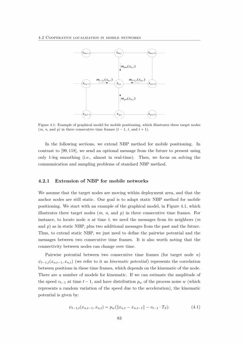
4.2 Cooperative localization in mobile networks
, 1m tx −
, 1n tx −
, 1p tx −
,m tx
,n tx
,p tx
, 1m tx +
, 1n tx +
, 1p tx +
1, ,( )t t n tm x− 1, ,( )t t n tm x+
,( )pn n tm x
,( )mn n tm x
Figure 4.1: Example of graphical model for mobile positioning, which illustrates three target nodes(m, n, and p) in three consecutive time frames (t− 1, t, and t+ 1).
In the following sections, we extend NBP method for mobile positioning. Incontrast to [99, 118], we send an optional message from the future to present usingonly 1-leg smoothing (i.e., almost in real-time). Then, we focus on solving thecommunication and sampling problems of standard NBP method.
4.2.1 Extension of NBP for mobile networks
We assume that the target nodes are moving within deployment area, and that theanchor nodes are still static. Our goal is to adapt static NBP method for mobilepositioning. We start with an example of the graphical model, in Figure 4.1, whichillustrates three target nodes (m, n, and p) in three consecutive time frames. Forinstance, to locate node n at time t, we need the messages from its neighbors (mand p) as in static NBP, plus two additional messages from the past and the future.Thus, to extend static NBP, we just need to define the pairwise potential and themessages between two consecutive time frames. It is also worth noting that theconnectivity between nodes can change over time.
Pairwise potential between two consecutive time frames (for target node n)ψt−1,t(xn,t−1, xn,t) (we refer to it as kinematic potential) represents the correlationbetween positions in these time frames, which depends on the kinematic of the node.There are a number of models for kinematic. If we can estimate the amplitude ofthe speed vt−1 at time t− 1, and have distribution pw of the process noise w (whichrepresents a random variation of the speed due to the acceleration), the kinematicpotential is given by:
ψt−1,t(xn,t−1, xn,t) = pw(‖xn,t − xn,t−1‖ − vt−1 · TS). (4.1)
83
Cooperative mobile network localization and tracking
where Ts represents the sampling interval. Note that it is usually hard to measurethe process noise (see Chapter 5), so Gaussian approximation is a common choice.However, since we prefer to keep non-Gaussian nature of NBP, we apply a simplermodel (as in [8]) which only requires the knowledge of the maximum speed of thetarget Vmax. This is usually easy to find for most applications (e.g., 5 m/s for people,1 m/s for forklifts, 30 m/s for cars, etc.). Given Vmax, kinematic potential of noden can be written as:
ψt−1,t(xn,t−1, xn,t) ={
1, if ‖xn,t−1 − xn,t‖ ≤ Vmax · Ts,0, otherwise.
(4.2)
Using this potential, we can predict the possible positions of node n at time t, giventhe estimate at time t−1, and vice versa for smoothing. Note that, if we can measurethe dynamic of the target (e.g., using an accelerometer or a pedometer), we can usea more informative kinematic potential [118].
Now we can extend the BP method described in Section 3.2 for mobile networks.Denote the belief of node n at time t, in last iteration of static BP (see (3.7)), asMSn,t(xn,t). To adapt the graphical model to mobile networks (according to Figure
4.1 and equation (3.7)), we can write the belief of node n in mobile networks as:
MFSn,t (xn,t) = mt−1,t(xn,t)MS
n,t(xn,t)mt+1,t(xn,t) = MFn,t(xn,t)mt+1,t(xn,t) (4.3)
where mt−1,t(xn,t) represents the filtering message (i.e., the message from pastto present), mt+1,t(xn,t) the smoothing message (i.e., the message from future topresent), and MFS
n,t (xn,t) is the belief which includes the filtering and the smoothingmessages. This belief can be available after Nt time frames (for Nt-leg smooth-ing). We will focus on 1-leg smoothing which can provide MFS
n,t (xn,t) at time t+ 1.By excluding mt+1,t(xn,t), we can also define the filtered belief MF
n,t(xn,t) which isavailable in real-time.
Using message update rule (see eq. (3.8)), we can define the filtering message(from t−1 to t), and the smoothing message (from t+1 to t). They are, respectively,given by:
mt−1,t(xn,t) ∝ˆ
xn,t−1
ψt−1,t(xn,t−1, xn,t)MFSn,t−1(xn,t−1)
mt,t−1(xn,t−1) dxn,t−1 (4.4)
mt+1,t(xn,t) ∝ˆ
xn,t+1
ψt+1,t(xn,t+1, xn,t)MFSn,t+1(xn,t+1)
mt,t+1(xn,t+1) dxn,t+1 (4.5)
84
4.2 Cooperative localization in mobile networks
Using (4.3), we can simplify previous equations:
mt−1,t(xn,t) ∝ˆ
xn,t−1
ψt−1,t(xn,t−1, xn,t)MFn,t−1(xn,t−1)dxn,t−1 (4.6)
mt+1,t(xn,t) ∝ˆ
xn,t+1
ψt+1,t(xn,t+1, xn,t)MSn,t+1(xn,t+1)mt+2,t+1(xn,t+1)dxn,t+1 (4.7)
Moreover, since we prefer to use 1-leg smoothing, we discard further informationfrom the future (i.e., we set mt+2,t+1(xn,t+1) = 1):
mt+1,t(xn,t) ∝ˆ
xn,t+1
ψt+1,t(xn,t+1, xn,t)MSn,t+1(xn,t+1)dxn,t+1 (4.8)
Regarding nonparametric approximation, we can reuse the weighted particlesfrom the static scenario {WS,j
n,t , XS,jn,t } (see Section 3.3), and use the filtering and the
smoothing message to reweight them:
WFS,jn,t = mt−1,t(XS,j
n,t ) ·WS,jn,t ·mt+1,t(XS,j
n,t ) = WF,jn,t ·mt+1,t(XS,j
n,t ) (4.9)
Messages, (4.6) and (4.8), can be computed via Monte Carlo integration, i.e.:
mt−1,t(xn,t) ∝∑j
ψt−1,t(XS,jn,t−1, xn,t)W
F,jn,t−1 (4.10)
mt+1,t(xn,t) ∝∑j
ψt+1,t(XS,jn,t+1, xn,t)W
S,jn,t+1 (4.11)
As we can see, this method is very flexible, since there are three different beliefsavailable: MS
n,t, MFn,t, and MFS
n,t . The belief MFn,t should be used in real-time ap-
plications, while the belief MFSn,t should be used in all applications in which we can
afford waiting one more sampling interval (TS). On the other hand, the belief MSn,t
should not be used for tracking, but it is useful for testing the target dynamic (forexample, it can be used to learn Vmax, if not known in advance).
Finally, it is important to mention that the proposed extension of NBP is notexact in networks with loops. As explained in Chapter 3, it can cause overconfidentbeliefs of the position estimates. This problem, which is inherited from the staticnetworks, can be solved using all proposed solutions in Chapter 3. However, in thischapter, we consider the networks with a negligible number of loops, so NBP-basedmethods will be good enough for the all analyses.
85
Cooperative mobile network localization and tracking
4.2.2 A novel communication protocol
Our second goal is to decrease the communication cost of NBP by: i) broadcastingthe beliefs instead of the messages, ii) approximating the packages without a signi-ficant effect on the localization performance, and iii) avoiding the transmission ofuninformative data. The proposed solutions are applicable for the mobile as well asfor the static networks (Chapter 3).
Broadcasting beliefs
Naturally, one can assume that the messages should be transmitted between eachpairs of the neighboring nodes. However, this produce a huge communication over-head since each node would need to send one message to each of the neighbors.Obviously, the main problem of this approach is that it does not take advantage ofthe broadcast in WSN (i.e., the transmitted message is needed at just one neighbor,not all). If we recall equation (see (3.9) in Chapter 3), we can see that the particlesof the messages are constructed using particles from the: i) current belief of the nodewhich transmits the message (source node), ii) measured distance, and iii) randomangle. Since the samples of the distance can be measured by each node (prior tolocalization) and stored into memory, they should not be transmitted. The samplesof the angles are drawn from the uniform distribution (3.9), so they can be computedat the destination. Thus, only particles of the beliefs, which are not available at thedestination node, should be transmitted. One problem could be reweighting (3.10),using outgoing message from previous iteration, since each node has only incomingmessages. It can be solved by computing the messages twice: once at the sourcenode, and once at the destination node. This protocol is summarized in Alg 8.
The main benefit of this approach is that each node has to broadcast only onepackage1 instead of nd packages in case of message transmission (where nd is nodedegree). This is paid by slight increase in computation since the messages must becomputed twice. However, it is already well-known [76] that the communication ismuch more energy-consuming than computation.
Package Approximation
For the described protocol, we would need to transmit Np particles (i.e., Np weights,and 2Np coordinates). However, we can avoid this using the following approxima-tions:
1To avoid confusion, we use term “packages” for the scalar data that will be transmitted, incontrast to term “messages” which refers to NBP messages, which are never transmitted. For thisanalysis, the package contains only one scalar value.
86

4.2 Cooperative localization in mobile networks
Algorithm 8 Communication protocol (without approximation and censoring)1: for all nodes do2: Obtain sufficient number of distance samples (from each neighbor)3: Initialize all belief and messages (see Section 3.2 in Chapter 3)4: for all iterations do5: Compute particles from outgoing messages and reweight them6: Transmit particles of the current belief7: Compute particles from incoming messages and reweight them8: end for9: end for
• We resample with replacement before transmission in order to avoid transmis-sion of the weights.
• The bandwidth (3.11) can be computed using the unweighted set of particles[13,46], so it should not be transmitted.
• We approximate unweighted particles with Gaussian mixture, and transmitonly their parameters. Upon receiving, we re-draw the set of particles fromthis mixture.
Since first two approximations are already part of the standard NBP (see Section3.3.2), they do not affect accuracy. Regarding the last approximation, we expect that(given sufficient mixture components) it will not affect significantly the localizationperformance. Since the main problem of cooperative localization is the presence ofmulti-modal beliefs (caused by non-rigid graphs and/or multi-modal measurementnoise), we expect that Gaussian mixture of very few components is appropriatechoice. We can cluster unweighted set of particles using k-means algorithm [59], orexpectation-maximization (see [9], chapter 9). The latter one can provide slightlybetter results, but with higher complexity. Thus, we recommend the use of k-means,especially for mobile networks.
Package censoring
We can additionally decrease communication using package censoring, i.e., by avoid-ing the transmission of the packages which provide little information. To that end,we do the following:
• In the first iteration, we only transmit the bounds of the bounded box (i.e.,4 scalar values, which define the rectangle) (see Section 3.3.4). Then, theparticles can be drawn at the destination node.
87
Cooperative mobile network localization and tracking
• We do not transmit beliefs in the last iterations since they will never be usedto update messages.
• Packages from anchor nodes are never transmitted (except their coordinates,if not known in advance).
• We do not transmit beliefs at iteration i which are similar to the beliefs initeration i− 1. The similarity can be measured using the KL divergence.
• We do not transmit parameters of mixture components which have very smallweights (less than some predefined threshold).
We expect that these steps will, without any effect on accuracy, significantlydecrease the communication cost. Note that we can also avoid receiving packages,as done in [26]. This technique should be applied if receiving the data is energy-consuming, and also in the case of single-cast communication.
4.2.3 Improving sampling techniques
In this section, our goal is to improve the sampling techniques used in standardNBP. We propose three techniques: i) MIS with reference particles (MIS-RP), ii)PMC, and iii) the method based on an auxiliary variable.
MIS-RP
The MIS technique defined by (3.16) usually provides a very good set of particles,and outperforms a number of techniques as shown in [47, 48]. However, this mightnot be the case in some rare events, e.g., in the presence of the huge outliers (e.g.,if obstacles are moving around).
According to the results in mobile robot localization [36], it is always useful to adda small number of uniformly distributed particles. These particles are essential for re-localization in the rare event that the sensor loses track of its position. We call theseadditional particles, reference particles (RP). In our case, this will especially happenif the messages from the neighboring target nodes provide wrong particles, buteither anchor nodes or the kinematic message provide good weights. The problemis illustrated in Figure 4.2. Without RP (Figure 4.2a), MIS provides the set ofparticles in which the best candidate is very far from the true position (e.g., due tothe outliers). With RP (Figure 4.2b), additional particles have been added uniformlyin the whole area, so the best candidate is closer2 to the true position.
2To simplify the example, we assumed the MAP estimate, but the same conclusion is valid forthe MMSE estimate.
88
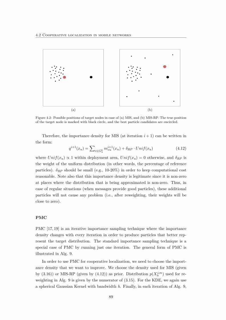
4.2 Cooperative localization in mobile networks
(a) (b)
Figure 4.2: Possible positions of target nodes in case of (a) MIS, and (b) MIS-RP. The true positionof the target node is marked with black circle, and the best particle candidates are encircled.
Therefore, the importance density for MIS (at iteration i+ 1) can be written inthe form:
qi+1(xu) =∑
v∈G0u
mi+1vu (xu) + δRP · Unif(xu) (4.12)
where Unif(xu) ∝ 1 within deployment area, Unif(xu) = 0 otherwise, and δRP isthe weight of the uniform distribution (in other words, the percentage of referenceparticles). δRP should be small (e.g., 10-20%) in order to keep computational costreasonable. Note also that this importance density is legitimate since it is non-zeroat places where the distribution that is being approximated is non-zero. Thus, incase of regular situations (when messages provide good particles), these additionalparticles will not cause any problem (i.e., after reweighting, their weights will beclose to zero).
PMC
PMC [17, 19] is an iterative importance sampling technique where the importancedensity changes with every iteration in order to produce particles that better rep-resent the target distribution. The standard importance sampling technique is aspecial case of PMC by running just one iteration. The general form of PMC isillustrated in Alg. 9.
In order to use PMC for cooperative localization, we need to choose the import-ance density that we want to improve. We choose the density used for MIS (givenby (3.16)) or MIS-RP (given by (4.12)) as prior. Distribution p(Xj,m
u ) used for re-weighting in Alg. 9 is given by the numerator of (3.15). For the KDE, we again usea spherical Gaussian Kernel with bandwidth h. Finally, in each iteration of Alg. 9,
89
Cooperative mobile network localization and tracking
Algorithm 9 Population Monte Carlo (PMC) (for node u)1: Choose initial importance function: q1
u(xu)2: for all iterations m = 1 : Nm do3: Draw particles: Xj,m
u ∼ qmu (x) (j = 1...Np)4: Compute weights: W j,m
u = p(Xj,mu )
qmu (Xj,mu )
5: Normalize weights: W j,mu = W j,m
u∑jW
(m)u
6: Resample with replacement7: Update importance density: qm+1
u (xu) =∑j Kh(xu −Xj,m
u )8: end for
we can draw a new set of the particles from this kernel as follows:
Xj,mu = Xj,m−1
u + εju · [cos(θju) sin(θju)] (4.13)
where εju ∼ N(ε; 0, h) and θju ∼ Unif [0, 2π). Note that we used simplified notationby removing the NBP iteration (do not mix NBP iterations with PMC iterations).We refer to this version of NBP, as PMC-NBP.
Finally, we propose an optional approximation of the PMC-NBP method. Themain computational problem of NBP and variations is the computation of KDE,which requires O(N2
p ) operations. This is especially the problem in PMC-NBP, sinceit has nested iterations (i.e., within one NBP iteration, there are NPMC iterations).Therefore, instead of using full information (the product of the messages from allthe neighbors), we use only information from the anchors. In order to keep the NBPalgorithm regular, we just need to keep full information in the first iteration of thePMC (which corresponds to the standard importance sampling). Since we do not useinformation from the target nodes, this method represents a non-cooperative PMC.Note that this approach will not only improve the beliefs of the anchors’ neighbors.Since NBP is still a cooperative method, in NBP’s very next iteration, the improvedestimate of the anchors’ neighbors will be flooded further into the network.
Auxiliary variable
Standard importance sampling used in NBP does not take into account most of theavailable information in the graph. This often causes high variance of the weights,i.e. there will be a lot of particles in the regions of low probability, and very few(or even just one) in the regions of high probability. One solution to this problemis to use the optimal importance density, which includes all the available informa-tion, but this is not feasible in most cases [2]. A second solution is PMC from theprevious section, which iteratively improves the importance density. The auxiliary
90
4.2 Cooperative localization in mobile networks
particle filtering (APF) [35,81] is an alternative solution which tries to predict (usingauxiliary variable) which particles will be in regions of high probability.
However, NBP is a generalization of particle filtering for any graphical model,so we need to adapt the standard APF method. One framework has been alreadyproposed in [16], in which the authors propose to use the index of the messages asan auxiliary variable in order to predict which message provides better information.This method is not very suitable (especially, for localization) due to the high dimen-sional auxiliary variable. In contrast to this approach, we will choose a 1D auxiliaryvariable, which will provide the largest amount of information.
Let us recall equation (3.9), written in a more general form:
xjru = XjXr + (dru + vjd)[cos(θjθ) sin(θjθ)] (4.14)
in which we again removed the NBP iteration index and, in contrast to (3.9), we usea different index (j, jX , jd, jθ ∼ 1...Np) for each random variable. As we can see, toupdate the particles of the messages (xjru), we need to use three random variables:particles of the current position (XjX
r ∼Mr(xr)), distance samples (dru + vjd ∼ pv),and angle samples (θjθ ∼ Unif [0, 2π)). The auxiliary variable could be an indexof any of these three random variables. Obviously, the uniformly distributed θjθ
includes the smallest amount of information (the entropy is maximal) than anyother random variable, so we choose jθ as the auxiliary variable. Then, we can setthe other indices to the same value (jX = jd = j). In other words, instead of drawingsamples uniformly in any direction (which will create a lot of particles with smallweights), we will draw them in the most likely direction according to the distributionof the auxiliary variable. To achieve this, we first, for each index jθ, find some likelyvalue associated with the message, e.g., expected value:
µjθru = µXr + µdru [cos(θjθ) sin(θjθ)] (4.15)
where we averaged the left-hand side of (4.14) over j. The computed set of meanvalues is further used to compute first-stage (1st) weights:
wjθ,1stru ∝ p(Y |µjθru) (4.16)
which represent the likelihood function given all information (Y ) that we want toinclude. Recall that these weights are for the message from node r to node u, whichrepresents some information about position of node u. Thus, we can include theproduct of all the messages coming to node u, but as for PMC, we again restrict toinformation from the anchors. For this approach, it is even more critical because the
91
Cooperative mobile network localization and tracking
number of messages (equal to twice the number of the edges in the graph) is typicallysignificantly larger than the number of target nodes. Therefore, the likelihood ofthe information that we want to include is given by:
p(Y |µjθru) =∏
a∈Gap(dau|x∗a, µjθru) ∝
∏a∈Ga
ψau(x∗a, µjθru) (4.17)
where Ga is the set of all the anchor neighbors of node u. In case of no anchorsin the neighborhood, we simply do not apply this approach. First-stage weightsprovide us information on how likely is the index of the angle jθ. Therefore, giventhe multinomial distribution defined by first-stage weights, we can draw set of Np
indices ind(jθ) (jθ = 1...Np). Then, we can compute particles from the message:
xjθru = Xjθr + (dru + vjθ)[sin(θind(jθ)) cos(θind(jθ))] (4.18)
Finally, the whole procedure is still not regular due to the double-counting of theinformation from anchors (which is regularly used in (3.15)). Thus, the regularweights, given by (3.10), should be divided by the weights of the importance densitygiven by the first-stage weights (4.16). The final weights for the particles from themessage, also called the second-stage weights [81] are given by:
wjθru = W jθr
mur(Xjθr )· 1p(Y |µind(jθ)
ru )(4.19)
Given these weights, we can proceed with the standard NBP. We refer to this versionas auxiliary NBP (ANBP). It is worth noting that the standard NBP is a special caseof ANBP, if no additional information (Y ) has been used, i.e., when p(Y |µjθru) ∝ 1,and p(θind(jθ)) = p(θjθ) ∝ Unif [0, 2π).
4.2.4 Simulation results
We conducted several simulations to analyse the performance of the NBP method inmobile networks, the effect of package approximation and censoring, and the effectof the improved sampling techniques.
Analysis of mobile positioning based on NBP
In first set of tests, we assume that there are Na = 16 anchor nodes and Nt = 5target nodes, deployed in a 100m x 100m area. Anchor nodes are deployed in grid,or semi-random3 topology. Target nodes are moving according to the Gaussian-
3The area is divided into Na square-shaped cells, and each anchor node is deployed randomlywithin one of them (i.e., one anchor per cell).
92
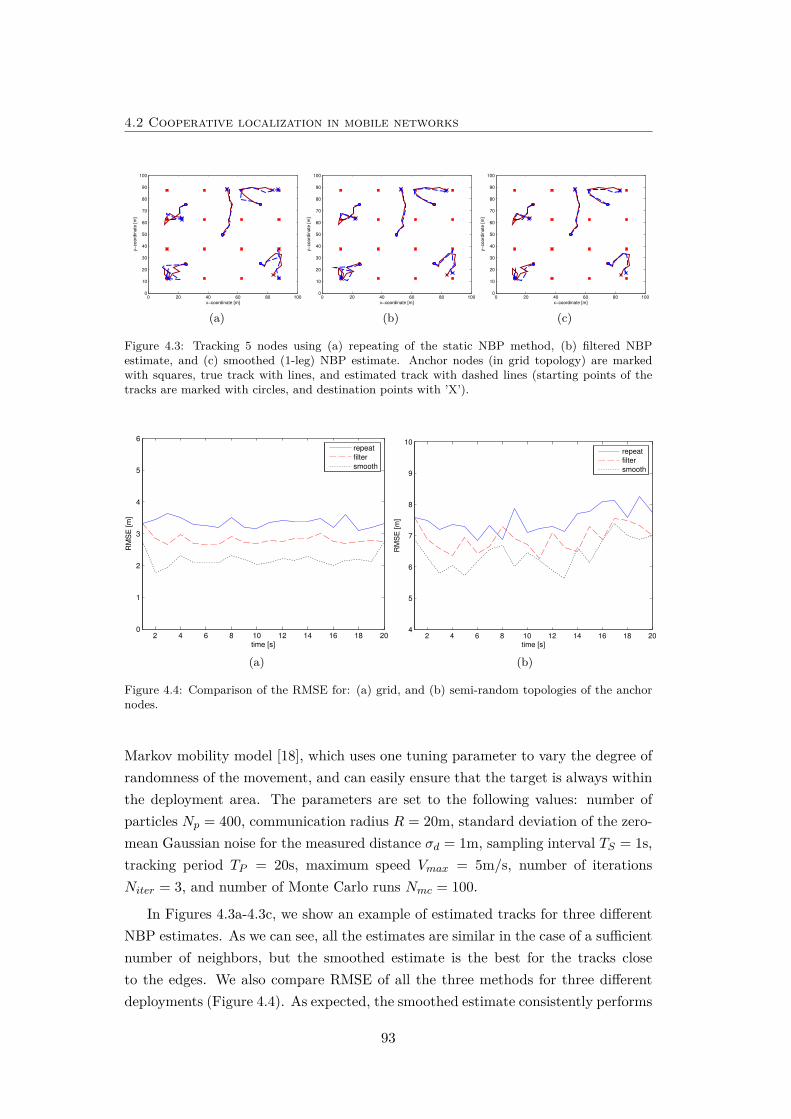
4.2 Cooperative localization in mobile networks
0 20 40 60 80 1000
10
20
30
40
50
60
70
80
90
100
x−coordinate [m]
y−
co
ord
ina
te [
m]
(a)
0 20 40 60 80 1000
10
20
30
40
50
60
70
80
90
100
x−coordinate [m]y−
co
ord
ina
te [
m]
(b)
0 20 40 60 80 1000
10
20
30
40
50
60
70
80
90
100
x−coordinate [m]
y−
co
ord
ina
te [
m]
(c)
Figure 4.3: Tracking 5 nodes using (a) repeating of the static NBP method, (b) filtered NBPestimate, and (c) smoothed (1-leg) NBP estimate. Anchor nodes (in grid topology) are markedwith squares, true track with lines, and estimated track with dashed lines (starting points of thetracks are marked with circles, and destination points with ’X’).
2 4 6 8 10 12 14 16 18 200
1
2
3
4
5
6
time [s]
RM
SE
[m
]
repeat
filter
smooth
(a)
2 4 6 8 10 12 14 16 18 204
5
6
7
8
9
10
time [s]
RM
SE
[m
]
repeat
filter
smooth
(b)
Figure 4.4: Comparison of the RMSE for: (a) grid, and (b) semi-random topologies of the anchornodes.
Markov mobility model [18], which uses one tuning parameter to vary the degree ofrandomness of the movement, and can easily ensure that the target is always withinthe deployment area. The parameters are set to the following values: number ofparticles Np = 400, communication radius R = 20m, standard deviation of the zero-mean Gaussian noise for the measured distance σd = 1m, sampling interval TS = 1s,tracking period TP = 20s, maximum speed Vmax = 5m/s, number of iterationsNiter = 3, and number of Monte Carlo runs Nmc = 100.
In Figures 4.3a-4.3c, we show an example of estimated tracks for three differentNBP estimates. As we can see, all the estimates are similar in the case of a sufficientnumber of neighbors, but the smoothed estimate is the best for the tracks closeto the edges. We also compare RMSE of all the three methods for three differentdeployments (Figure 4.4). As expected, the smoothed estimate consistently performs
93
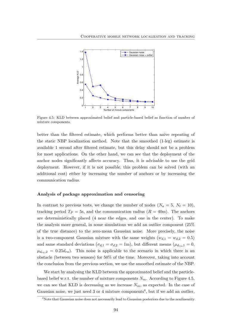
Cooperative mobile network localization and tracking
1 2 3 4 5 6 7 8 9 100
0.2
0.4
0.6
0.8
1
1.2
1.4
Number of mixture components
Avera
ge K
LD
Gaussian noise
Gaussian noise + outlier
Figure 4.5: KLD between approximated belief and particle-based belief as function of number ofmixture components.
better than the filtered estimate, which performs better than naive repeating ofthe static NBP localization method. Note that the smoothed (1-leg) estimate isavailable 1 second after filtered estimate, but this delay should not be a problemfor most applications. On the other hand, we can see that the deployment of theanchor nodes significantly affects accuracy. Thus, it is advisable to use the griddeployment. However, if it is not possible, this problem can be solved (with anadditional cost) either by increasing the number of anchors or by increasing thecommunication radius.
Analysis of package approximation and censoring
In contrast to previous tests, we change the number of nodes (Na = 5, Nt = 10),tracking period TP = 5s, and the communication radius (R = 40m). The anchorsare deterministically placed (4 near the edges, and one in the center). To makethe analysis more general, in some simulations we add an outlier component (25%of the true distance) to the zero-mean Gaussian noise. More precisely, the noiseis a two-component Gaussian mixture with the same weights (wd,1 = wd,2 = 0.5)and same standard deviations (σd,1 = σd,2 = 1m), but different means (µdru,1 = 0,µdru,2 = 0.25dru). This noise is applicable to the scenario in which there is anobstacle (between two sensors) for 50% of the time. Moreover, taking into accountthe conclusion from the previous section, we use the smoothed estimate of the NBP.
We start by analysing the KLD between the approximated belief and the particle-based belief w.r.t. the number of mixture components Nm. According to Figure 4.5,we can see that KLD is decreasing as we increase Nm, as expected. In the case ofGaussian noise, we just need 3 or 4 mixture components4, but if we add an outlier,
4Note that Gaussian noise does not necessarily lead to Gaussian posteriors due to the nonlinearity
94
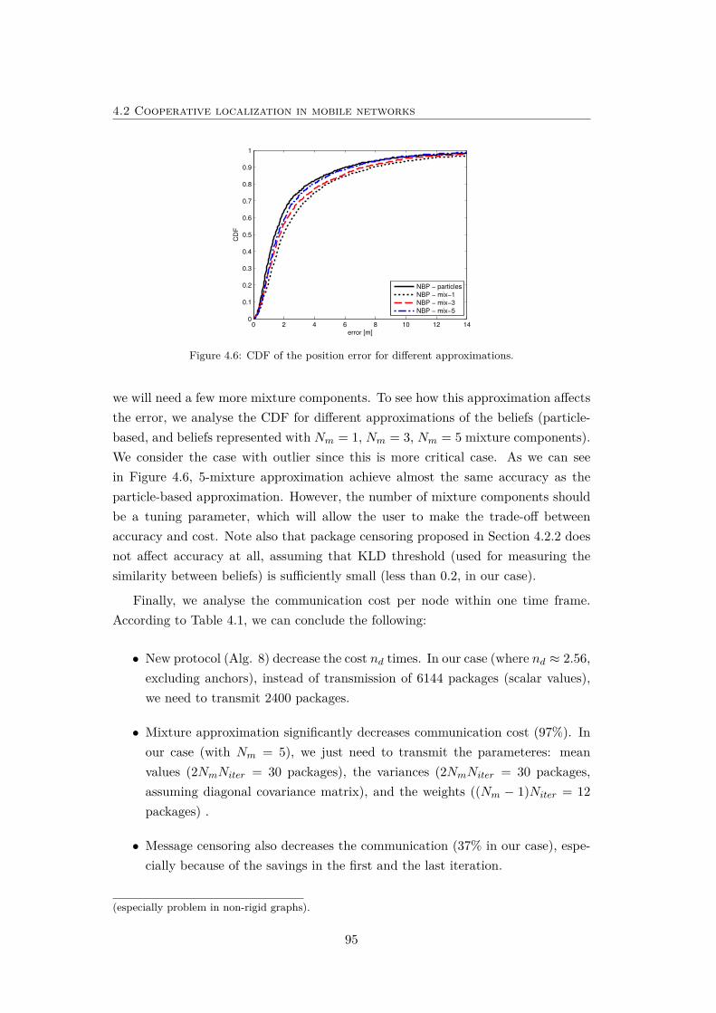
4.2 Cooperative localization in mobile networks
0 2 4 6 8 10 12 140
0.1
0.2
0.3
0.4
0.5
0.6
0.7
0.8
0.9
1
error [m]
CD
F
NBP − particles
NBP − mix−1
NBP − mix−3
NBP − mix−5
Figure 4.6: CDF of the position error for different approximations.
we will need a few more mixture components. To see how this approximation affectsthe error, we analyse the CDF for different approximations of the beliefs (particle-based, and beliefs represented with Nm = 1, Nm = 3, Nm = 5 mixture components).We consider the case with outlier since this is more critical case. As we can seein Figure 4.6, 5-mixture approximation achieve almost the same accuracy as theparticle-based approximation. However, the number of mixture components shouldbe a tuning parameter, which will allow the user to make the trade-off betweenaccuracy and cost. Note also that package censoring proposed in Section 4.2.2 doesnot affect accuracy at all, assuming that KLD threshold (used for measuring thesimilarity between beliefs) is sufficiently small (less than 0.2, in our case).
Finally, we analyse the communication cost per node within one time frame.According to Table 4.1, we can conclude the following:
• New protocol (Alg. 8) decrease the cost nd times. In our case (where nd ≈ 2.56,excluding anchors), instead of transmission of 6144 packages (scalar values),we need to transmit 2400 packages.
• Mixture approximation significantly decreases communication cost (97%). Inour case (with Nm = 5), we just need to transmit the parameteres: meanvalues (2NmNiter = 30 packages), the variances (2NmNiter = 30 packages,assuming diagonal covariance matrix), and the weights ((Nm − 1)Niter = 12packages) .
• Message censoring also decreases the communication (37% in our case), espe-cially because of the savings in the first and the last iteration.
(especially problem in non-rigid graphs).
95
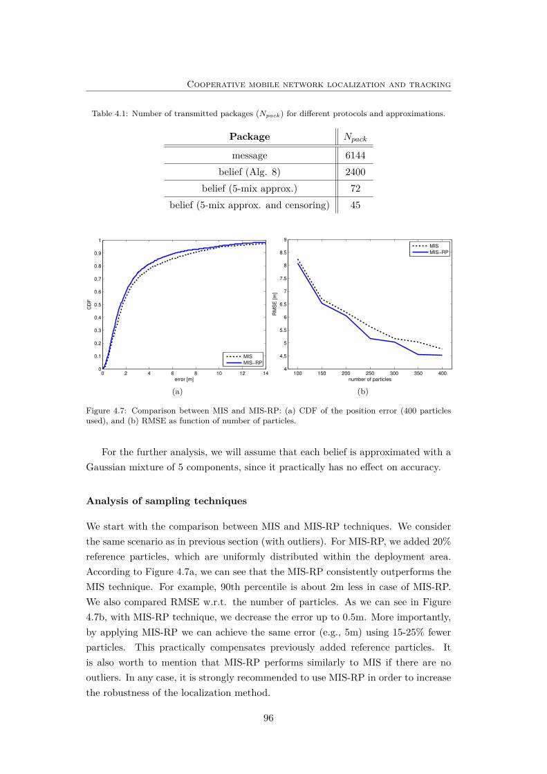
Cooperative mobile network localization and tracking
Table 4.1: Number of transmitted packages (Npack) for different protocols and approximations.
Package Npack
message 6144belief (Alg. 8) 2400
belief (5-mix approx.) 72belief (5-mix approx. and censoring) 45
0 2 4 6 8 10 12 140
0.1
0.2
0.3
0.4
0.5
0.6
0.7
0.8
0.9
1
error [m]
CD
F
MIS
MIS−RP
(a)
100 150 200 250 300 350 4004
4.5
5
5.5
6
6.5
7
7.5
8
8.5
9
number of particles
RM
SE
[m
]
MIS
MIS−RP
(b)
Figure 4.7: Comparison between MIS and MIS-RP: (a) CDF of the position error (400 particlesused), and (b) RMSE as function of number of particles.
For the further analysis, we will assume that each belief is approximated with aGaussian mixture of 5 components, since it practically has no effect on accuracy.
Analysis of sampling techniques
We start with the comparison between MIS and MIS-RP techniques. We considerthe same scenario as in previous section (with outliers). For MIS-RP, we added 20%reference particles, which are uniformly distributed within the deployment area.According to Figure 4.7a, we can see that the MIS-RP consistently outperforms theMIS technique. For example, 90th percentile is about 2m less in case of MIS-RP.We also compared RMSE w.r.t. the number of particles. As we can see in Figure4.7b, with MIS-RP technique, we decrease the error up to 0.5m. More importantly,by applying MIS-RP we can achieve the same error (e.g., 5m) using 15-25% fewerparticles. This practically compensates previously added reference particles. Itis also worth to mention that MIS-RP performs similarly to MIS if there are nooutliers. In any case, it is strongly recommended to use MIS-RP in order to increasethe robustness of the localization method.
96
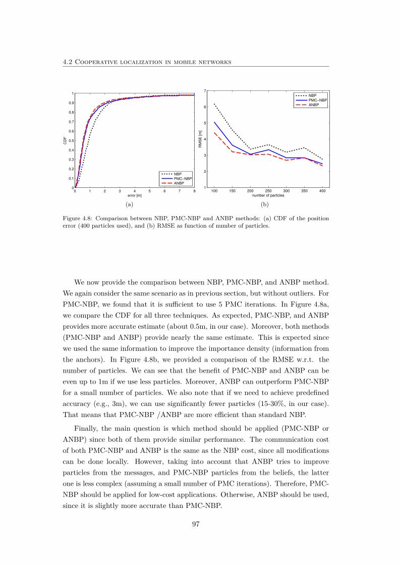
4.2 Cooperative localization in mobile networks
0 1 2 3 4 5 6 7 80
0.1
0.2
0.3
0.4
0.5
0.6
0.7
0.8
0.9
1
error [m]
CD
F
NBP
PMC−NBP
ANBP
(a)
100 150 200 250 300 350 4001
2
3
4
5
6
7
number of particlesR
MS
E [
m]
NBP
PMC−NBP
ANBP
(b)
Figure 4.8: Comparison between NBP, PMC-NBP and ANBP methods: (a) CDF of the positionerror (400 particles used), and (b) RMSE as function of number of particles.
We now provide the comparison between NBP, PMC-NBP, and ANBP method.We again consider the same scenario as in previous section, but without outliers. ForPMC-NBP, we found that it is sufficient to use 5 PMC iterations. In Figure 4.8a,we compare the CDF for all three techniques. As expected, PMC-NBP, and ANBPprovides more accurate estimate (about 0.5m, in our case). Moreover, both methods(PMC-NBP and ANBP) provide nearly the same estimate. This is expected sincewe used the same information to improve the importance density (information fromthe anchors). In Figure 4.8b, we provided a comparison of the RMSE w.r.t. thenumber of particles. We can see that the benefit of PMC-NBP and ANBP can beeven up to 1m if we use less particles. Moreover, ANBP can outperform PMC-NBPfor a small number of particles. We also note that if we need to achieve predefinedaccuracy (e.g., 3m), we can use significantly fewer particles (15-30%, in our case).That means that PMC-NBP /ANBP are more efficient than standard NBP.
Finally, the main question is which method should be applied (PMC-NBP orANBP) since both of them provide similar performance. The communication costof both PMC-NBP and ANBP is the same as the NBP cost, since all modificationscan be done locally. However, taking into account that ANBP tries to improveparticles from the messages, and PMC-NBP particles from the beliefs, the latterone is less complex (assuming a small number of PMC iterations). Therefore, PMC-NBP should be applied for low-cost applications. Otherwise, ANBP should be used,since it is slightly more accurate than PMC-NBP.
97
Cooperative mobile network localization and tracking
4.3 Distributed target tracking
Distributed tracking5 in WSN is important tasks for many applications in whichcentral unit is not available. For example, in emergency situations, such as fireor nuclear disaster, WSN can be deployed to detect these phenomena. Once thephenomena is detected (e.g., increased temperature, or radioactivity), the sensorsstart to sense their neighborhood and cooperatively track people and assets. Assensors are low-cost devices that may not survive during deployment, it is importantto achieve tracking in a manner that is fully asynchronous and robust to sensorsfailures, and in such a way that every sensor has the same belief of the targetlocation. Moreover, due to the nonlinear relationships and possible non-Gaussianuncertainties, a particle filtering (PF) should be applied [2], instead of traditionalmethods based on Kalman filtering (KF) [116].
Most of the methods for PF-based distributed target tracking in WSN are basedon the construction and maintenance of the communication path. For example,in [22], low-power sensors pass the parameters of likelihood function to the high-power sensors, which are responsible to manage the low-power nodes. In [103],a set of uncorrelated sensor cliques is constructed, in which slave nodes have totransmit Gaussian mixture parameters to the master node of the clique. Master nodeperforms the tracking, and forward estimates to another clique. In [62], a Markov-chain distributed PF is proposed, which does not route the information through thegraph during tracking. However, it requires that each node knows total number ofcommunication links and the number of communication links between each pair ofnodes, which can be obtained only by aggregating the data before tracking. These,routing-based6 algorithms lack robustness to failures and are also not suitable forasynchronous networks. To address these problems, several authors have consideredusing average consensus algorithms. In [41], the global posterior distribution isapproximated with a Gaussian mixture, and consensus is applied over the localparameters to compute the global parameters. Similarly, [42, 44] uses a Gaussianapproximation instead of Gaussian mixture. Randomized gossip consensus was usedin [74,106] for distributed target tracking. Finally, as a benchmark, we also mentionthe non-centralized PF (NCPF) [29], in which each node broadcasts measurementsuntil all the nodes have complete set of measurements. Then, each node (actinglike a fusion center) performs the tracking. Although this method is not scalable,it can be still competitive in some scenarios. These state-of-the-art methods suffer
5Note that distributed tracking is also cooperative. In order to be consistent with literature, wewill refer to it as distributed tracking.
6Authors sometimes use the term “message passing” [41, 42, 62] for this type of methods. Thiscan be confusing with the standard message passing method, belief propagation, which does notbelong to this category.
98
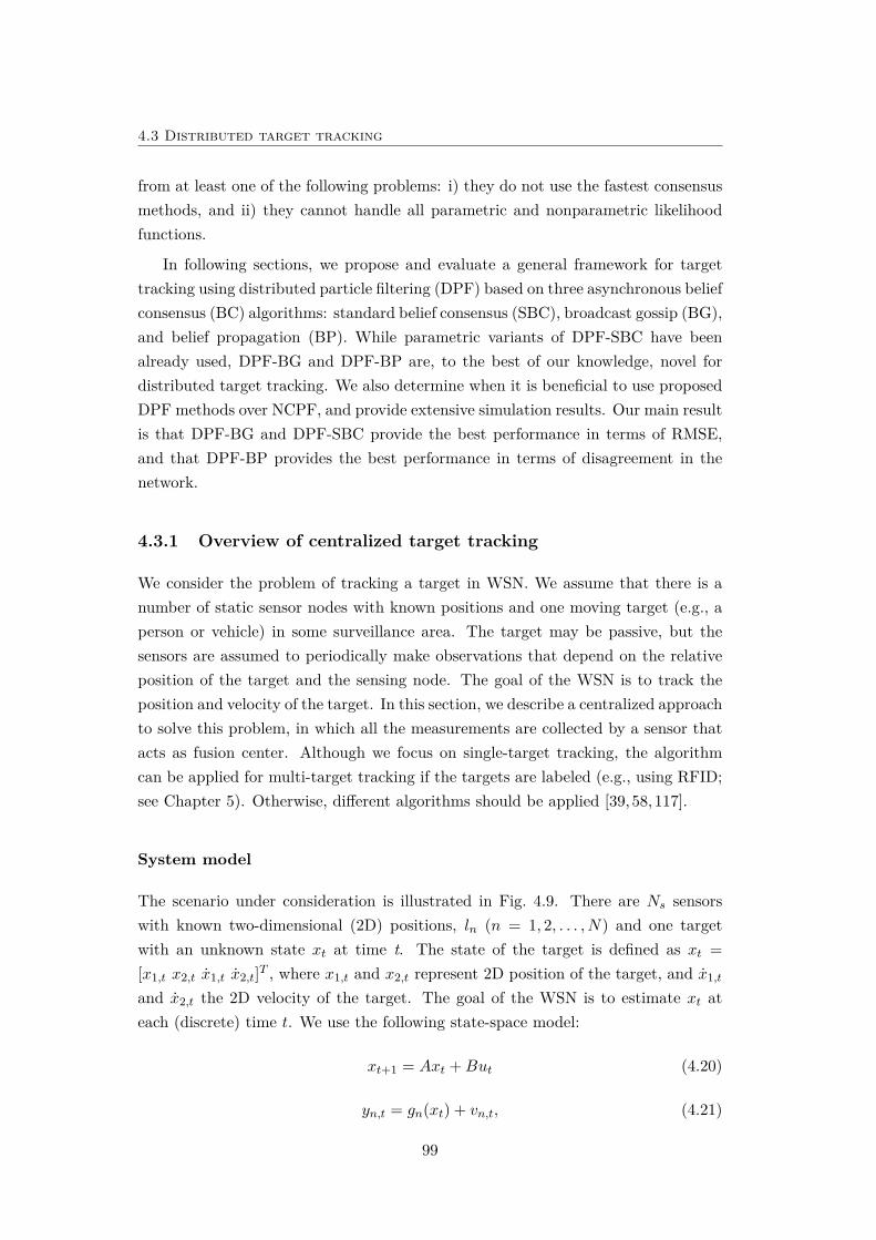
4.3 Distributed target tracking
from at least one of the following problems: i) they do not use the fastest consensusmethods, and ii) they cannot handle all parametric and nonparametric likelihoodfunctions.
In following sections, we propose and evaluate a general framework for targettracking using distributed particle filtering (DPF) based on three asynchronous beliefconsensus (BC) algorithms: standard belief consensus (SBC), broadcast gossip (BG),and belief propagation (BP). While parametric variants of DPF-SBC have beenalready used, DPF-BG and DPF-BP are, to the best of our knowledge, novel fordistributed target tracking. We also determine when it is beneficial to use proposedDPF methods over NCPF, and provide extensive simulation results. Our main resultis that DPF-BG and DPF-SBC provide the best performance in terms of RMSE,and that DPF-BP provides the best performance in terms of disagreement in thenetwork.
4.3.1 Overview of centralized target tracking
We consider the problem of tracking a target in WSN. We assume that there is anumber of static sensor nodes with known positions and one moving target (e.g., aperson or vehicle) in some surveillance area. The target may be passive, but thesensors are assumed to periodically make observations that depend on the relativeposition of the target and the sensing node. The goal of the WSN is to track theposition and velocity of the target. In this section, we describe a centralized approachto solve this problem, in which all the measurements are collected by a sensor thatacts as fusion center. Although we focus on single-target tracking, the algorithmcan be applied for multi-target tracking if the targets are labeled (e.g., using RFID;see Chapter 5). Otherwise, different algorithms should be applied [39,58,117].
System model
The scenario under consideration is illustrated in Fig. 4.9. There are Ns sensorswith known two-dimensional (2D) positions, ln (n = 1, 2, . . . , N) and one targetwith an unknown state xt at time t. The state of the target is defined as xt =[x1,t x2,t x1,t x2,t]T , where x1,t and x2,t represent 2D position of the target, and x1,t
and x2,t the 2D velocity of the target. The goal of the WSN is to estimate xt ateach (discrete) time t. We use the following state-space model:
xt+1 = Axt +But (4.20)
yn,t = gn(xt) + vn,t, (4.21)
99
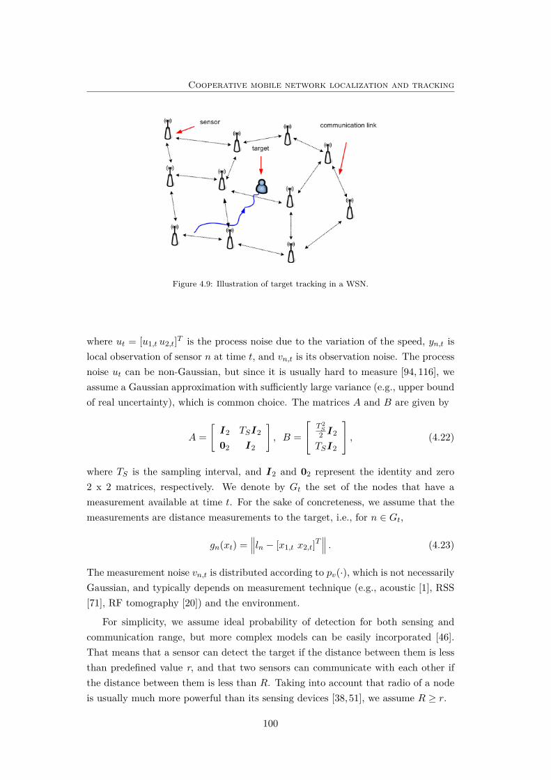
Cooperative mobile network localization and tracking
Figure 4.9: Illustration of target tracking in a WSN.
where ut = [u1,t u2,t]T is the process noise due to the variation of the speed, yn,t islocal observation of sensor n at time t, and vn,t is its observation noise. The processnoise ut can be non-Gaussian, but since it is usually hard to measure [94, 116], weassume a Gaussian approximation with sufficiently large variance (e.g., upper boundof real uncertainty), which is common choice. The matrices A and B are given by
A =[
I 2 TSI 2
02 I 2
], B =
T 2S2 I 2
TSI 2
, (4.22)
where TS is the sampling interval, and I 2 and 02 represent the identity and zero2 x 2 matrices, respectively. We denote by Gt the set of the nodes that have ameasurement available at time t. For the sake of concreteness, we assume that themeasurements are distance measurements to the target, i.e., for n ∈ Gt,
gn(xt) =∥∥∥ln − [x1,t x2,t]T
∥∥∥ . (4.23)
The measurement noise vn,t is distributed according to pv(·), which is not necessarilyGaussian, and typically depends on measurement technique (e.g., acoustic [1], RSS[71], RF tomography [20]) and the environment.
For simplicity, we assume ideal probability of detection for both sensing andcommunication range, but more complex models can be easily incorporated [46].That means that a sensor can detect the target if the distance between them is lessthan predefined value r, and that two sensors can communicate with each other ifthe distance between them is less than R. Taking into account that radio of a nodeis usually much more powerful than its sensing devices [38,51], we assume R ≥ r.
100
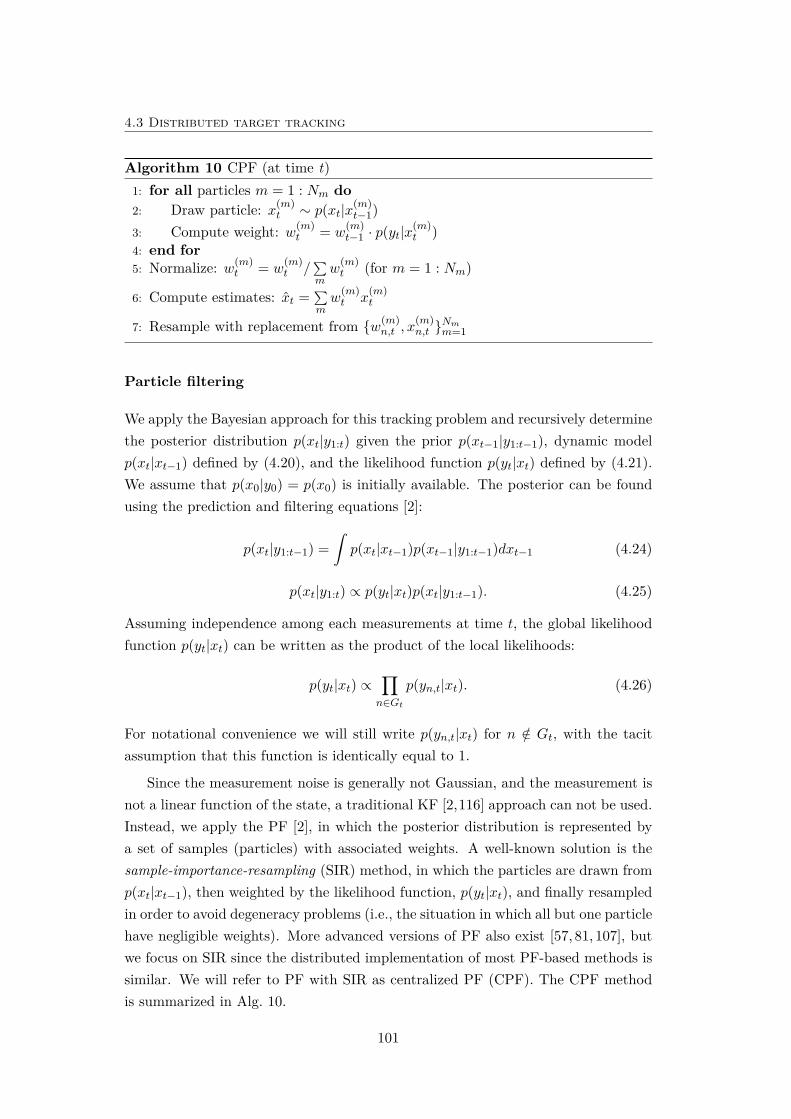
4.3 Distributed target tracking
Algorithm 10 CPF (at time t)1: for all particles m = 1 : Nm do2: Draw particle: x(m)
t ∼ p(xt|x(m)t−1)
3: Compute weight: w(m)t = w
(m)t−1 · p(yt|x
(m)t )
4: end for5: Normalize: w(m)
t = w(m)t /
∑mw
(m)t (for m = 1 : Nm)
6: Compute estimates: xt =∑mw
(m)t x
(m)t
7: Resample with replacement from {w(m)n,t , x
(m)n,t }
Nmm=1
Particle filtering
We apply the Bayesian approach for this tracking problem and recursively determinethe posterior distribution p(xt|y1:t) given the prior p(xt−1|y1:t−1), dynamic modelp(xt|xt−1) defined by (4.20), and the likelihood function p(yt|xt) defined by (4.21).We assume that p(x0|y0) = p(x0) is initially available. The posterior can be foundusing the prediction and filtering equations [2]:
p(xt|y1:t−1) =ˆp(xt|xt−1)p(xt−1|y1:t−1)dxt−1 (4.24)
p(xt|y1:t) ∝ p(yt|xt)p(xt|y1:t−1). (4.25)
Assuming independence among each measurements at time t, the global likelihoodfunction p(yt|xt) can be written as the product of the local likelihoods:
p(yt|xt) ∝∏n∈Gt
p(yn,t|xt). (4.26)
For notational convenience we will still write p(yn,t|xt) for n /∈ Gt, with the tacitassumption that this function is identically equal to 1.
Since the measurement noise is generally not Gaussian, and the measurement isnot a linear function of the state, a traditional KF [2,116] approach can not be used.Instead, we apply the PF [2], in which the posterior distribution is represented bya set of samples (particles) with associated weights. A well-known solution is thesample-importance-resampling (SIR) method, in which the particles are drawn fromp(xt|xt−1), then weighted by the likelihood function, p(yt|xt), and finally resampledin order to avoid degeneracy problems (i.e., the situation in which all but one particlehave negligible weights). More advanced versions of PF also exist [57, 81, 107], butwe focus on SIR since the distributed implementation of most PF-based methods issimilar. We will refer to PF with SIR as centralized PF (CPF). The CPF methodis summarized in Alg. 10.
101
Cooperative mobile network localization and tracking
This algorithm is run on one of the nodes in the WSN, which serves as fusioncenter. The main drawbacks of the CPF are: i) large energy consumption on thenodes which are in proximity of the fusion center, ii) high communication cost inlarge-scale networks; iii) the posterior distribution cannot be accessed from anynode in the network; and iv) fusion center has to know the locations, observations,and observation models of all the nodes. In the following section we will focus ondistributed implementations of PF method, which alleviate these problems.
4.3.2 Distributed particle filtering
Our goal is to track the target in a distributed, asynchronous way, such that all thenodes have a common view of the state of the target. We use distributed implement-ation of the PF (DPF), in which we want to avoid exchanging measurements and tohave a common set of samples and weights at every time step. If we can guaranteethat the samples at time t− 1 are common, and the weights at time t are common,then common samples at time t can be achieved by providing all nodes with thesame seed for random number generation, so as to ensure that their pseudo-randomgenerators are in the same state at all times. Ensuring common weights for all nodescan be achieved by means of a BC algorithm. BC formally aims to compute, in adistributed fashion the product of a number of functions over the same variable
BC(f1(x), f2(x), . . . , fNs(x)) =Ns∏n=1
fn(x). (4.27)
However, most BC algorithms are not capable to achieve exact consensus in a finitenumber of iterations (except BP-consensus in tree-like graphs; see Section 4.3.3). Aswe require exact consensus on the weights, we additionally apply max-consensus7
(MC) [72,106],MC(f1(x), f2(x), . . . , fNs(x)) = max
nfn(x), (4.28)
which computes the exact maximum over all arguments using the same asynchronousprotocol as average consensus in a finite number of iterations (equal to the diameterof the graph). This idea has been already used in [106] for gossip-based consensus.The final algorithm is shown in Alg. 11. Observe that, in contrast to CPF, thefollowing drawbacks have been removed: i) energy consumption is balanced acrossthe network; ii) reduced communication cost in certain scenarios (see later in thechapter); iii) every node has access to the posterior distribution; and iv) no know-ledge required of the locations, observations, or observation models of any othernode.
7Min-consensus can be also applied.
102
4.3 Distributed target tracking
Algorithm 11 DPF (at node n, at time t)1: for all particles m = 1 : Nm do2: Draw particle: x(m)
t ∼ p(xn,t|x(m)t−1)
3: Compute weight: w(m)n,t =
w(m)t−1 · BC
(p(y1,t|x(m)
t ), ..., p(yNs,t|x(m)t )
)4: end for5: Normalize: w(m)
n,t = w(m)n,t /
∑mw
(m)n,t (for m = 1 : Nm)
6: Compute estimates: xn,t =∑mw
(m)n,t x
(m)n,t
7: w(m)t = MC
(w
(m)1,t , ..., w
(m)Ns,t
)(for m = 1 : Nm)
8: Normalize: w(m)t = w
(m)t /
∑mw
(m)t (for m = 1 : Nm)
9: Resample with replacement from {w(m)t , x
(m)t }
Nmm=1
In the next section, we will describe three distinct BC algorithms.
4.3.3 Belief consensus algorithms
Our goal is to approximate the product of the local likelihoods using BC algorithms.Motivated by their scalability, asynchronous behavior and robustness to failures[6,24,73], we consider three variants of BC: SBC [73], BC based on BG [6], and BCbased on BP [24,77].
SBC
SBC [73] is defined in following iterative form:
M (i)n (xt) = M (i−1)
n (xt)∏u∈Gn
(M
(i−1)u (xt)
M(i−1)n (xt)
)ε, (4.29)
where Gn is the set of neighbors of node n,M (i)n represents current estimate (at itera-
tion i) of the global likelihood of the variable xt (in our case, xt ∈ {x(1)t , . . . , x
(Nm)t }),
and ε depends on maximum node degree in the network (0 < ε < 1/ηmax, whereηmax is maximum node degree in the network). For convenience, we define the up-date rate ξ (0 < ξ < 1), so ε = ξ/ηmax. Update rate ξ ≈ 1 is expected to provide thefastest convergence [72]. Note that logarithm of (4.29) represents standard averageconsensus algorithm [72]. We initialize by
M (1)n (xt) = p(yn,t|xt). (4.30)
103
Cooperative mobile network localization and tracking
This consensus algorithm guarantees convergence (in all connected graphs) as num-ber of iterations goes to infinity [73]. Thus, it asymptotically converges to thegeometrical average of the local distributions:
limi→∞
M (i)n (xt) =
∏n∈Gt
p(yn,t|xt)
1/Ns
, (4.31)
from which the desired quantity,∏n∈Gt p(yn,t|xt), can easily be found, for any value
of xt ∈ {x(1)t , . . . , x
(Nm)t }.
If the maximum node degree (ηmax) and number of nodes (Ns) are not known apriori, we need to estimate them in distributed way. The estimation of maximumnode degree can be done using max-consensus, while Ns can be determined [80] bysetting the initial state of one node to 1, and all others to 0. By using averageconsensus [72], they can obtain the result 1/Ns, which is the inverse of the numberof nodes in the network. We refer to this method as DPF-SBC.
BC based on BG
Gossip-based algorithms [28] can also achieve consensus in asynchronous networks.In order to use the broadcast nature of WSN, we choose broadcast gossip (BG) [6].It has been shown [6] that this method is significantly faster than other well-knowngossip-based methods, such as randomized gossip [15], and geographic gossip [27], inwhich only one pair of the nodes update its state per iteration. In broadcast gossip, itis assumed that all the nodes has internal clock which ticks independently accordingto a rate of e.g., a Poisson process [6]. When the clock of the n-th node ticks, noden broadcasts its own state value. This state value is received by all neighbors withincommunication radius R. Then, these nodes will make weighted average of theircurrent state value and the received state value. It has been shown [6] that BGconverges, in expectation, to the real average value.
For the belief consensus, we need to achieve convergence to the geometricalaverage (4.31), so at the k-th clock tick of node n all the nodes make the followingoperation:
M (k)u (xt) =
M(k−1)u (xt)γM (k−1)
n (xt)1−γ , u ∈ GnM
(k−1)u (xt), otherwise
(4.32)
where 0 < γ < 1 is the mixing parameter. It has been shown [6] that optimal valueof γ depends on the algebraic connectivity of the graph (which represent the secondsmallest eigenvalue of the Laplacian matrix [6, 72]). However, this parameter is notavailable in distributed scenario, so empirical study has been used [6] to find the
104
4.3 Distributed target tracking
optimal value of γ. Therefore, we will model γ as function of average node degree ηin the network, since η can be easily estimated in distributed way.
Initialization is exactly the same as for SBC. We also need to apply averageconsensus to estimate Ns and η. We refer to this variant of DPF as DPF-BG.
However, we make one difference comparing with standard BG. In order to havethe same communication cost per iteration, we assume that one SBC iteration cor-responds to Ns BG iterations (i.e., i = dk/Nse). This assumption is reasonabletaking into account that, to avoid collisions, even SBC has to broadcast its data insequential way.
BC based on BP
BP is well-known message passing algorithm on an undirected graphical model (see[24,77] and Chapter 3). Consider the following function:
∏n
p(yn,t|xn,t)∏u∈Gn
δ(xn,t − xu,t), (4.33)
which is equal to∏n∈Gt p(yn,t|xt), whenever all the dummy variables are the same.
Comparing (4.33) with (3.6)8, we can see that, if we set pairwise potential todelta Dirac impulse, running BP on the corresponding graph yields the margin-als Mn(xn,t) = C
∏n p(yn,t|xn,t) for every n, where C is a normalization constant.
Note that this normalization constant is irrelevant as weights in Alg. 11 will be nor-malized later anyway. The BP message passing equations are now as follows: thebelief at iteration i (the current approximation of C
∏n p(yn,t|xn,t)) is, according to
(3.7), given by:M (i)n (xn,t) ∝ p(yn,t|xn,t)
∏u∈Gn
m(i)un(xn,t), (4.34)
while the message from node u ∈ Gn to node n is, according to (3.8), given by:
m(i)un(xn,t) ∝
ˆxu,t
δ(xn,t − xu,t)M
(i−1)u (xu,t)
m(i−1)nu (xu,t)
dxu,t = M(i−1)u (xn,t)
m(i−1)nu (xn,t)
. (4.35)
Previous equation (4.35), can be written as:
m(i)un(xt) ∝
M(i−1)u (xt)
m(i−1)nu (xt)
, (4.36)
8Note that, in this chapter, t is time index, in contrast to Chapter 3.
105
Cooperative mobile network localization and tracking
where we removed index n since all the nodes have the same variable (xn,t = xu,t =xt). The denominator of (4.36) is the message from node n to node u in the previousiteration, and can be expressed as
m(i−1)nu (xt) ∝
M(i−2)n (xt)
m(i−2)un (xt)
. (4.37)
Combining previous two equations, we get the recursive expression for the messages:
m(i)un(xt) ∝
M(i−1)u (xt)
M(i−2)n (xt)
m(i−2)un (xt) (4.38)
Combining (4.34) and (4.38), we find a recursive expression for the beliefs:
M (i)n (xt) ∝ p(yn,t|xt)
∏u∈Gn
(M
(i−1)u (xt)
M(i−2)n (xt)
m(i−2)un (xt)
)(4.39)
= p(yn,t|xt)∏u∈Gn
m(i−2)un (xt)
∏u∈Gn
(M
(i−1)u (xt)
M(i−2)n (xt)
)
= M (i−2)n (xt)
∏u∈Gn
(M
(i−1)u (xt)
M(i−2)n (xt)
). (4.40)
which represents novel consensus algorithm based on BP. This method is initializedbyM (1)
n (xt) = p(yn,t|xt). We also need to setM (2)n (xt) in order to run the algorithm
defined by (4.40). Using (4.34) and (4.35), and assuming that m(1)nu (xt) = 1, we find
M (2)n (xt) = p(yn,t|xt)
∏u∈Gn
p(yu,t|xt) (4.41)
As described in Chapter 3, this method guarantees convergence to C∏n p(yn,t|xt)
for cycle-free network graphs. When the network graph has cycles, the beliefs areonly approximations of the true marginals (more details in Appendix B). Comparing(4.40) and (4.29), we can see that SBC is not specific instance of BP. In contrastto SBC, BP-consensus agrees on product of all local evidences (not the Ns-th rootof the product), and does not rely on knowledge of ηmax and Ns. We refer to thisvariant of DPF as DPF-BP.
Communication cost analysis
In this section, we analyze the communication cost of the three DPF methods, andcompare with the cost of NCPF and CPF. We denote by Npack the number of packets
106
4.3 Distributed target tracking
that a generic node n broadcasts at a generic time t. We assume that one packetcan contain P scalar values. We neglect the cost of determining (ηmax, η and Ns),so that all DPF methods will have the same communication cost.
At every iteration (except the first), nodes transmit Nw weights. In addition,nodes must perform MC, which also requires transmission of the weights in eachiteration. The number of iterations of the BC is Nit. The number of iterations ofthe MC is equal to the to the diameter of the graph Dg, which represents maximumhop-distance between two nodes. Thus, the average cost of DPF per node and pertime slot is
NDPFpack ≈
⌈Nw
P
⌉(Dg +Nit − 1). (4.42)
NCPF does not require transmission of the weights, but only local data, i.e., itsobservations and its 2D position9. We denote the number of these scalar values asNdata. The amount of data will accumulate with iterations since the node has totransmit its own data and all received data. Since the number of iterations is equalto Dg, the cost can be approximated by:
NNCPFpack ≈
Dg−1∑k=0
⌈ηkNdataP
⌉, (4.43)
where we approximate the degree of the each node with average network degree (η).
The cost of CPF depends on many factors, including the routing protocol, andthe position of the fusion center. Taking into account that in CPF each node trans-mits its information once (in contrast of Dg times, in NCPF), and that the fusioncenter is on an edge of the area, the average cost can be roughly approximated with
NCPFpack ≈
NNCPFpackDg
. (4.44)
Note that this cost is not evenly distributed over network.
From (4.42) we see that the DPF methods are fully scalable, since increasing thenumber of the nodes (by increasing its density) will not affect the cost. Althoughbeyond the scope of this chapter, we mention that if one prefers to use parametricapproximations [41, 42, 44] instead of Nw messages, only parameters of the beliefsand 2D sensor positions should be transmitted, in each iteration. It is also possibleto transmit only large weights (larger than predefined threshold) as in [106], or useother techniques for weight compression.
9If all the sensors learn the measurement model online, learned parameters also have to betransmitted.
107
Cooperative mobile network localization and tracking
Making the reasonable assumption that Nit = Dg + 1, we can quantify whenDPF is preferred over NCPF, i.e., when NDPF
pack < NNCPFpack :
⌈Nw
P
⌉<
12Dg
Dg−1∑k=0
⌈ηkNdataP
⌉. (4.45)
This condition is important in order to avoid over-using of consensus-based methods.For example, if the network is fully-connected (Dg = 1), or if the packet size is suffi-ciently large to afford transmission of all accumulated data (i.e., P > ηDg−1Ndata),NCPF should be applied. On the other hand, if the communication radius is verysmall (i.e., if Dg is very large), DPF methods should be applied. Note that a sim-ilar comparison can be done with CPF (i.e., using (4.42) and (4.44)), but note thatthe communication cost is not the unique reason why CPF method is not used (seeSection 4.3.1).
4.3.4 Simulation results
Simulation setup and performance measures
We assume that there are Ns = 25 sensors semi-randomly deployed in a 100mx 100m area: the area is divided into Ns square-shaped cells, and one sensor israndomly placed in each of them. The positions of these sensors are perfectly known.There is also one target in the area which is moving with constant speed V = 5m/saccording to a Gaussian random walk. An example of a track in a 25-node networkis shown in Figure 4.10. The sampling interval is set to Ts = 1s, and number ofthese intervals is set to Nt = 50. We set the sensing radius to r = 25m, and varythe communication radius R. We assume that the measured distance is distributedaccording to Gaussian mixture with two components, in which one component isoutlier. The parameters of this noise are set to following values: µd = (1m, 10m),σd = (1m, 1m) and wd = (0.75, 0.25). We use Np = 200 particles. The results areaveraged over Nmc = 100 Monte Carlo runs.
We will compare CPF, NCPF, and the three DPF methods (DPF-SBC, DPF-BG, and DPF-BP). We consider two performance metrics: RMSE in the positionerror erms, and, for DPF methods, the average disagreement in the position error edis.Introducing en,t,s as the target positioning error (i.e., Euclidean distance betweenthe true and estimated position of the target) at node n, at time t in simulation runs, we have:
erms =
√∑n,t,s e
2n,t,s
NsNtNmc, (4.46)
108
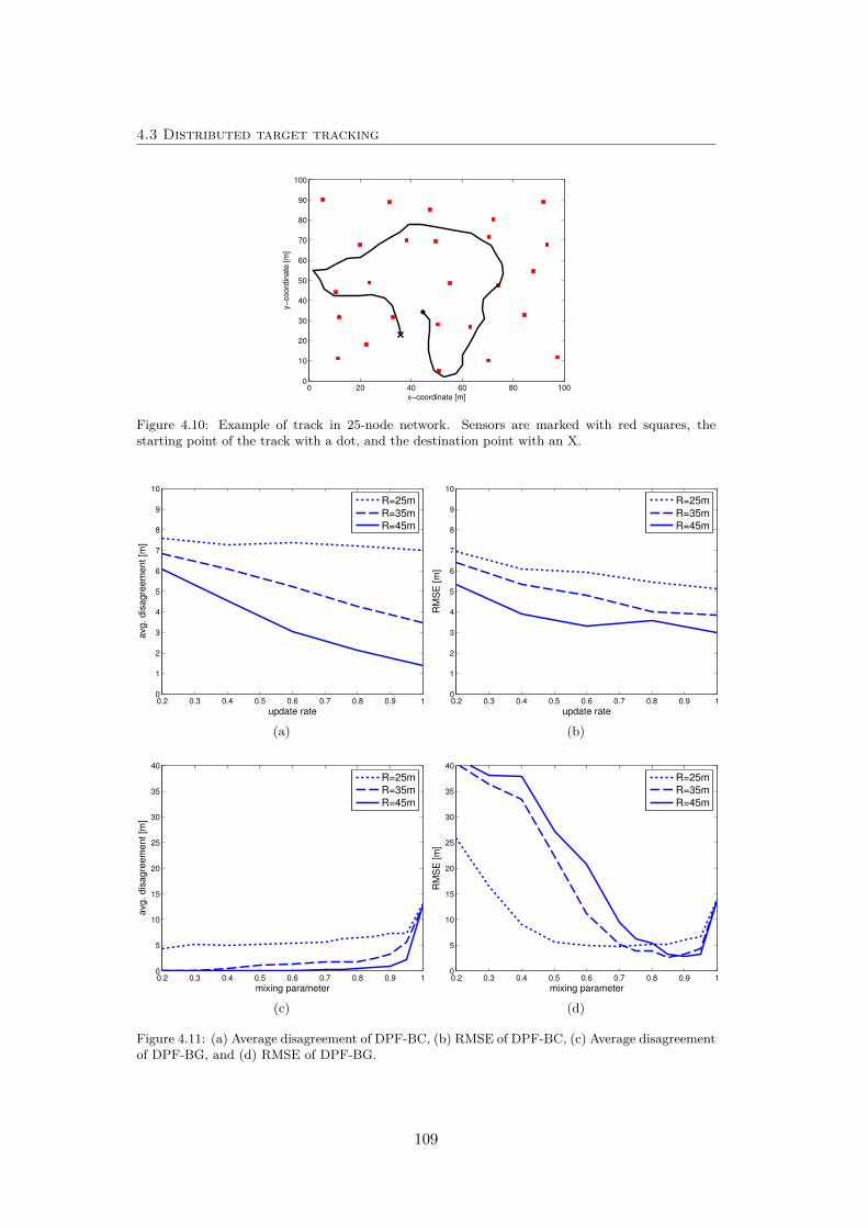
4.3 Distributed target tracking
0 20 40 60 80 1000
10
20
30
40
50
60
70
80
90
100
x−coordinate [m]
y−
co
ord
ina
te [
m]
Figure 4.10: Example of track in 25-node network. Sensors are marked with red squares, thestarting point of the track with a dot, and the destination point with an X.
0.2 0.3 0.4 0.5 0.6 0.7 0.8 0.9 10
1
2
3
4
5
6
7
8
9
10
update rate
avg
. d
isa
gre
em
en
t [m
]
R=25m
R=35m
R=45m
(a)
0.2 0.3 0.4 0.5 0.6 0.7 0.8 0.9 10
1
2
3
4
5
6
7
8
9
10
update rate
RM
SE
[m
]
R=25m
R=35m
R=45m
(b)
0.2 0.3 0.4 0.5 0.6 0.7 0.8 0.9 10
5
10
15
20
25
30
35
40
mixing parameter
avg
. d
isa
gre
em
en
t [m
]
R=25m
R=35m
R=45m
(c)
0.2 0.3 0.4 0.5 0.6 0.7 0.8 0.9 10
5
10
15
20
25
30
35
40
mixing parameter
RM
SE
[m
]
R=25m
R=35m
R=45m
(d)
Figure 4.11: (a) Average disagreement of DPF-BC, (b) RMSE of DPF-BC, (c) Average disagreementof DPF-BG, and (d) RMSE of DPF-BG.
109
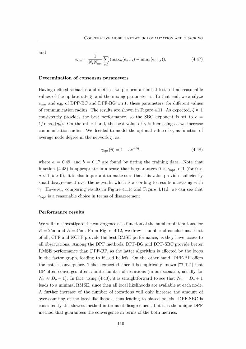
Cooperative mobile network localization and tracking
andedis = 1
NtNmc
∑s,t
(maxn(en,t,s)−minn(en,t,s)). (4.47)
Determination of consensus parameters
Having defined scenarios and metrics, we perform an initial test to find reasonablevalues of the update rate ξ, and the mixing parameter γ. To that end, we analyzeerms and edis of DPF-BC and DPF-BG w.r.t. these parameters, for different valuesof communication radius. The results are shown in Figure 4.11. As expected, ξ ≈ 1consistently provides the best performance, so the SBC exponent is set to ε =1/maxn(ηn). On the other hand, the best value of γ is increasing as we increasecommunication radius. We decided to model the optimal value of γ, as function ofaverage node degree in the network η, as:
γopt(η) = 1− ae−bη, (4.48)
where a = 0.49, and b = 0.17 are found by fitting the training data. Note thatfunction (4.48) is appropriate in a sense that it guarantees 0 < γopt < 1 (for 0 <
a < 1, b > 0). It is also important to make sure that this value provides sufficientlysmall disagreement over the network, which is according to results increasing withγ. However, comparing results in Figure 4.11c and Figure 4.11d, we can see thatγopt is a reasonable choice in terms of disagreement.
Performance results
We will first investigate the convergence as a function of the number of iterations, forR = 25m and R = 45m. From Figure 4.12, we draw a number of conclusions. Firstof all, CPF and NCPF provide the best RMSE performance, as they have access toall observations. Among the DPF methods, DPF-BG and DPF-SBC provide betterRMSE performance than DPF-BP, as the latter algorithm is affected by the loopsin the factor graph, leading to biased beliefs. On the other hand, DPF-BP offersthe fastest convergence. This is expected since it is empirically known [77,121] thatBP often converges after a finite number of iterations (in our scenario, usually forNit ≈ Dg + 1). In fact, using (4.40), it is straightforward to see that Nit = Dg + 1leads to a minimal RMSE, since then all local likelihoods are available at each node.A further increase of the number of iterations will only increase the amount ofover-counting of the local likelihoods, thus leading to biased beliefs. DPF-SBC isconsistently the slowest method in terms of disagreement, but it is the unique DPFmethod that guarantees the convergence in terms of the both metrics.
110
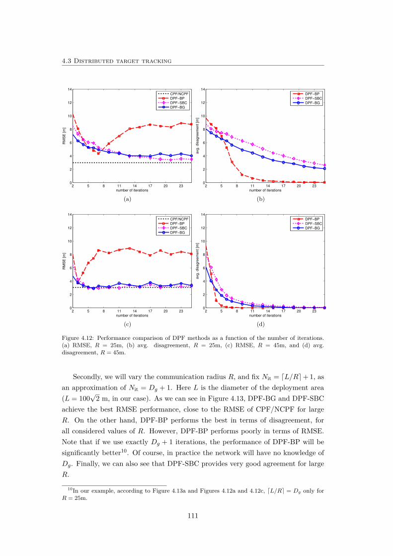
4.3 Distributed target tracking
2 5 8 11 14 17 20 230
2
4
6
8
10
12
14
number of iterations
RM
SE
[m
]
CPF/NCPF
DPF−BP
DPF−SBC
DPF−BG
(a)
2 5 8 11 14 17 20 230
2
4
6
8
10
12
14
number of iterations
avg. dis
agre
em
ent [m
]
DPF−BP
DPF−SBC
DPF−BG
(b)
2 5 8 11 14 17 20 230
2
4
6
8
10
12
14
number of iterations
RM
SE
[m
]
CPF/NCPF
DPF−BP
DPF−SBC
DPF−BG
(c)
2 5 8 11 14 17 20 230
2
4
6
8
10
12
14
number of iterations
avg. dis
agre
em
ent [m
]
DPF−BP
DPF−SBC
DPF−BG
(d)
Figure 4.12: Performance comparison of DPF methods as a function of the number of iterations.(a) RMSE, R = 25m, (b) avg. disagreement, R = 25m, (c) RMSE, R = 45m, and (d) avg.disagreement, R = 45m.
Secondly, we will vary the communication radius R, and fix Nit = dL/Re+ 1, asan approximation of Nit = Dg + 1. Here L is the diameter of the deployment area(L = 100
√2 m, in our case). As we can see in Figure 4.13, DPF-BG and DPF-SBC
achieve the best RMSE performance, close to the RMSE of CPF/NCPF for largeR. On the other hand, DPF-BP performs the best in terms of disagreement, forall considered values of R. However, DPF-BP performs poorly in terms of RMSE.Note that if we use exactly Dg + 1 iterations, the performance of DPF-BP will besignificantly better10. Of course, in practice the network will have no knowledge ofDg. Finally, we can also see that DPF-SBC provides very good agreement for largeR.
10In our example, according to Figure 4.13a and Figures 4.12a and 4.12c, dL/Re = Dg only forR = 25m.
111
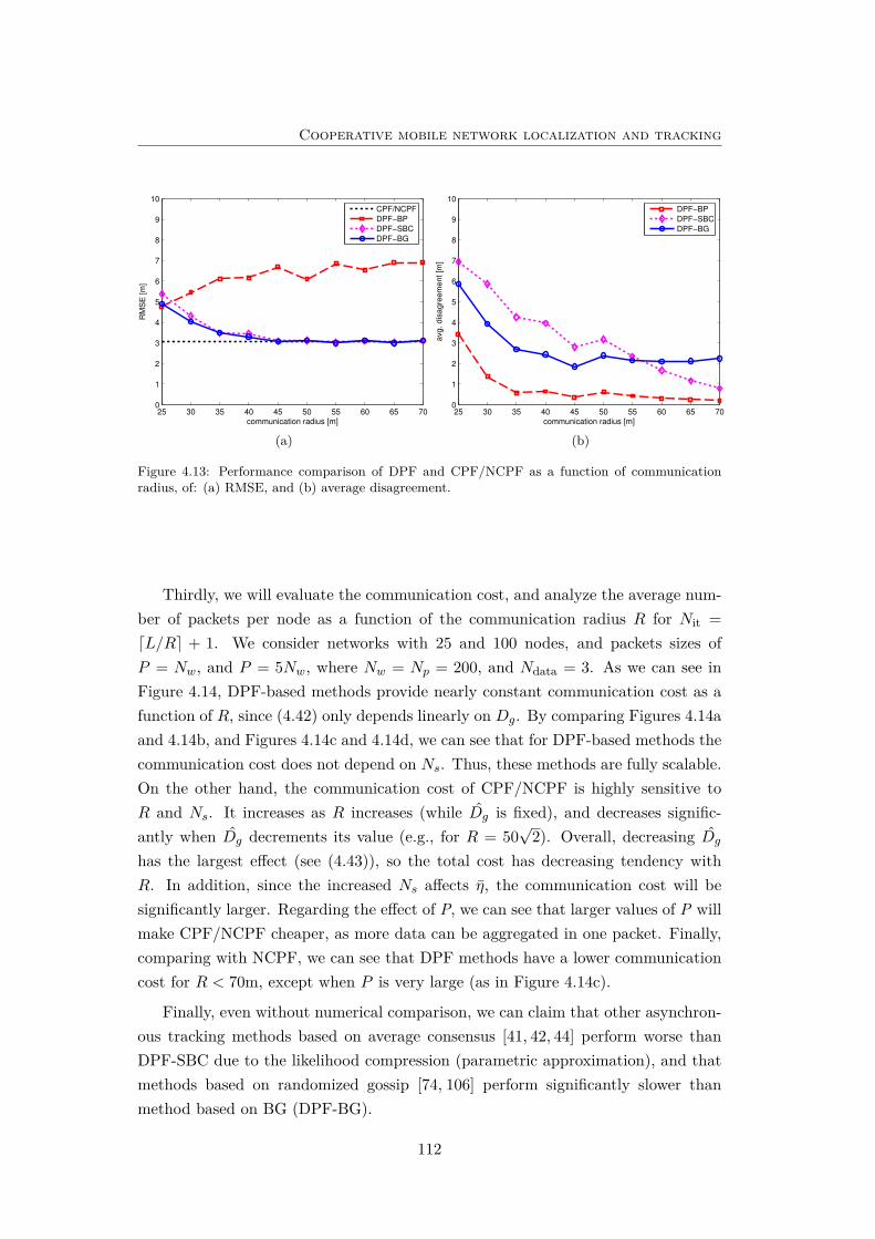
Cooperative mobile network localization and tracking
25 30 35 40 45 50 55 60 65 700
1
2
3
4
5
6
7
8
9
10
communication radius [m]
RM
SE
[m
]
CPF/NCPF
DPF−BP
DPF−SBC
DPF−BG
(a)
25 30 35 40 45 50 55 60 65 700
1
2
3
4
5
6
7
8
9
10
communication radius [m]
avg. dis
agre
em
ent [m
]
DPF−BP
DPF−SBC
DPF−BG
(b)
Figure 4.13: Performance comparison of DPF and CPF/NCPF as a function of communicationradius, of: (a) RMSE, and (b) average disagreement.
Thirdly, we will evaluate the communication cost, and analyze the average num-ber of packets per node as a function of the communication radius R for Nit =dL/Re + 1. We consider networks with 25 and 100 nodes, and packets sizes ofP = Nw, and P = 5Nw, where Nw = Np = 200, and Ndata = 3. As we can see inFigure 4.14, DPF-based methods provide nearly constant communication cost as afunction of R, since (4.42) only depends linearly on Dg. By comparing Figures 4.14aand 4.14b, and Figures 4.14c and 4.14d, we can see that for DPF-based methods thecommunication cost does not depend on Ns. Thus, these methods are fully scalable.On the other hand, the communication cost of CPF/NCPF is highly sensitive toR and Ns. It increases as R increases (while Dg is fixed), and decreases signific-antly when Dg decrements its value (e.g., for R = 50
√2). Overall, decreasing Dg
has the largest effect (see (4.43)), so the total cost has decreasing tendency withR. In addition, since the increased Ns affects η, the communication cost will besignificantly larger. Regarding the effect of P, we can see that larger values of P willmake CPF/NCPF cheaper, as more data can be aggregated in one packet. Finally,comparing with NCPF, we can see that DPF methods have a lower communicationcost for R < 70m, except when P is very large (as in Figure 4.14c).
Finally, even without numerical comparison, we can claim that other asynchron-ous tracking methods based on average consensus [41, 42, 44] perform worse thanDPF-SBC due to the likelihood compression (parametric approximation), and thatmethods based on randomized gossip [74, 106] perform significantly slower thanmethod based on BG (DPF-BG).
112
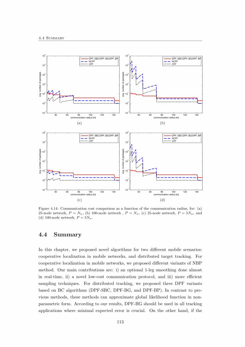
4.4 Summary
40 60 80 100 120 14010
−1
100
101
102
103
104
105
communication radius [m]
avg
. n
um
be
r o
f p
acka
ge
s
DPF−SBC/DPF−BG/DPF−BP
NCPF
CPF
(a)
40 60 80 100 120 14010
−1
100
101
102
103
104
105
communication radius [m]
avg
. n
um
be
r o
f p
acka
ge
s
DPF−SBC/DPF−BG/DPF−BP
NCPF
CPF
(b)
40 60 80 100 120 14010
−1
100
101
102
103
104
105
communication radius [m]
avg
. n
um
be
r o
f p
acka
ge
s
DPF−SBC/DPF−BG/DPF−BP
NCPF
CPF
(c)
40 60 80 100 120 14010
−1
100
101
102
103
104
105
communication radius [m]
avg
. n
um
be
r o
f p
acka
ge
s
DPF−SBC/DPF−BG/DPF−BP
NCPF
CPF
(d)
Figure 4.14: Communication cost comparison as a function of the communication radius, for: (a)25-node network, P = Nw, (b) 100-node network , P = Nw, (c) 25-node network, P = 5Nw, and(d) 100-node network, P = 5Nw.
4.4 Summary
In this chapter, we proposed novel algorithms for two different mobile scenarios:cooperative localization in mobile networks, and distributed target tracking. Forcooperative localization in mobile networks, we proposed different variants of NBPmethod. Our main contributions are: i) an optional 1-leg smoothing done almostin real-time, ii) a novel low-cost communication protocol, and iii) more efficientsampling techniques. For distributed tracking, we proposed three DPF variantsbased on BC algorithms (DPF-SBC, DPF-BG, and DPF-BP). In contrast to pre-vious methods, these methods can approximate global likelihood function in non-parametric form. According to our results, DPF-BG should be used in all trackingapplications where minimal expected error is crucial. On the other hand, if the
113

Cooperative mobile network localization and tracking
agreement of the estimates in the networks is more important than absolute error,DPF-BP could be a good choice. DPF-SBC, which guarantees convergence afterlarge number of iterations, could be applied when the cost and latency are notcrucial.
114
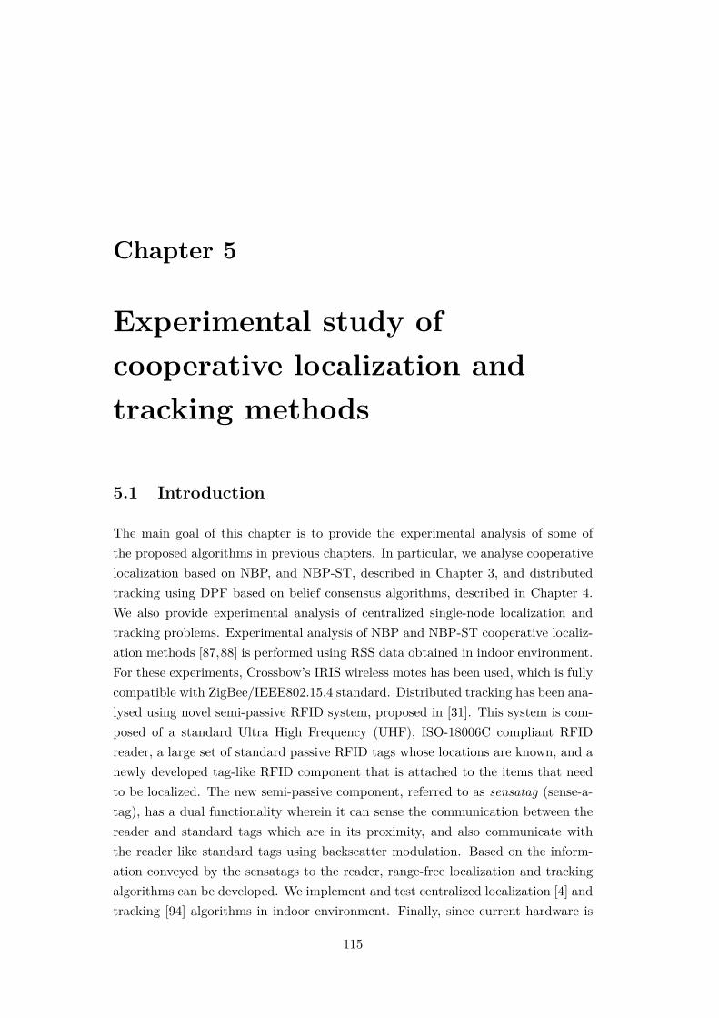
Chapter 5
Experimental study ofcooperative localization andtracking methods
5.1 Introduction
The main goal of this chapter is to provide the experimental analysis of some ofthe proposed algorithms in previous chapters. In particular, we analyse cooperativelocalization based on NBP, and NBP-ST, described in Chapter 3, and distributedtracking using DPF based on belief consensus algorithms, described in Chapter 4.We also provide experimental analysis of centralized single-node localization andtracking problems. Experimental analysis of NBP and NBP-ST cooperative localiz-ation methods [87,88] is performed using RSS data obtained in indoor environment.For these experiments, Crossbow’s IRIS wireless motes has been used, which is fullycompatible with ZigBee/IEEE802.15.4 standard. Distributed tracking has been ana-lysed using novel semi-passive RFID system, proposed in [31]. This system is com-posed of a standard Ultra High Frequency (UHF), ISO-18006C compliant RFIDreader, a large set of standard passive RFID tags whose locations are known, and anewly developed tag-like RFID component that is attached to the items that needto be localized. The new semi-passive component, referred to as sensatag (sense-a-tag), has a dual functionality wherein it can sense the communication between thereader and standard tags which are in its proximity, and also communicate withthe reader like standard tags using backscatter modulation. Based on the inform-ation conveyed by the sensatags to the reader, range-free localization and trackingalgorithms can be developed. We implement and test centralized localization [4] andtracking [94] algorithms in indoor environment. Finally, since current hardware is
115
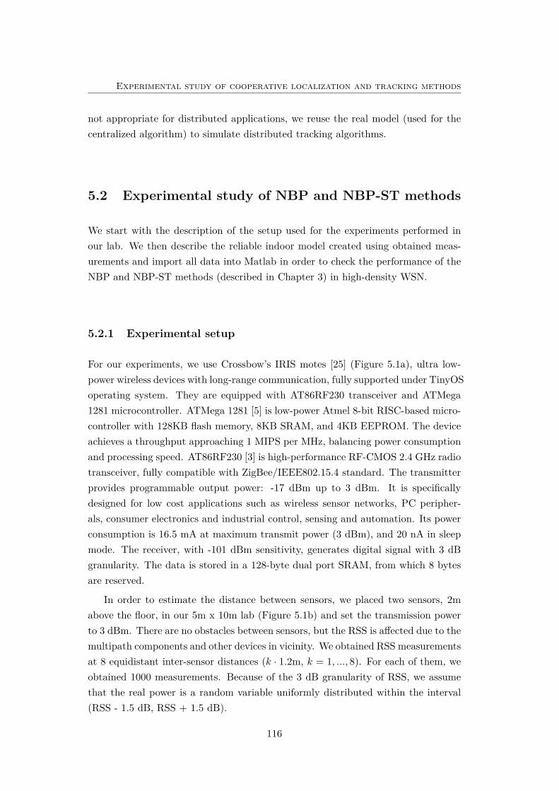
Experimental study of cooperative localization and tracking methods
not appropriate for distributed applications, we reuse the real model (used for thecentralized algorithm) to simulate distributed tracking algorithms.
5.2 Experimental study of NBP and NBP-ST methods
We start with the description of the setup used for the experiments performed inour lab. We then describe the reliable indoor model created using obtained meas-urements and import all data into Matlab in order to check the performance of theNBP and NBP-ST methods (described in Chapter 3) in high-density WSN.
5.2.1 Experimental setup
For our experiments, we use Crossbow’s IRIS motes [25] (Figure 5.1a), ultra low-power wireless devices with long-range communication, fully supported under TinyOSoperating system. They are equipped with AT86RF230 transceiver and ATMega1281 microcontroller. ATMega 1281 [5] is low-power Atmel 8-bit RISC-based micro-controller with 128KB flash memory, 8KB SRAM, and 4KB EEPROM. The deviceachieves a throughput approaching 1 MIPS per MHz, balancing power consumptionand processing speed. AT86RF230 [3] is high-performance RF-CMOS 2.4 GHz radiotransceiver, fully compatible with ZigBee/IEEE802.15.4 standard. The transmitterprovides programmable output power: -17 dBm up to 3 dBm. It is specificallydesigned for low cost applications such as wireless sensor networks, PC peripher-als, consumer electronics and industrial control, sensing and automation. Its powerconsumption is 16.5 mA at maximum transmit power (3 dBm), and 20 nA in sleepmode. The receiver, with -101 dBm sensitivity, generates digital signal with 3 dBgranularity. The data is stored in a 128-byte dual port SRAM, from which 8 bytesare reserved.
In order to estimate the distance between sensors, we placed two sensors, 2mabove the floor, in our 5m x 10m lab (Figure 5.1b) and set the transmission powerto 3 dBm. There are no obstacles between sensors, but the RSS is affected due to themultipath components and other devices in vicinity. We obtained RSS measurementsat 8 equidistant inter-sensor distances (k · 1.2m, k = 1, ..., 8). For each of them, weobtained 1000 measurements. Because of the 3 dB granularity of RSS, we assumethat the real power is a random variable uniformly distributed within the interval(RSS - 1.5 dB, RSS + 1.5 dB).
116
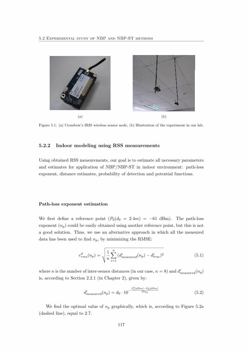
5.2 Experimental study of NBP and NBP-ST methods
(a) (b)
Figure 5.1: (a) Crossbow’s IRIS wireless sensor node, (b) Illustration of the experiment in our lab.
5.2.2 Indoor modeling using RSS measurements
Using obtained RSS measurements, our goal is to estimate all necessary parametersand estimates for application of NBP/NBP-ST in indoor environment: path-lossexponent, distance estimates, probability of detection and potential functions.
Path-loss exponent estimation
We first define a reference point (P0(d0 = 2.4m) = −61 dBm). The path-lossexponent (np) could be easily obtained using another reference point, but this is nota good solution. Thus, we use an alternative approach in which all the measureddata has been used to find np, by minimizing the RMSE:
edrms(np) =
√√√√ 1n
n∑i=1
(dimeasured(np)− ditrue)2 (5.1)
where n is the number of inter-sensor distances (in our case, n = 8) and dimeasured(np)is, according to Section 2.2.1 (in Chapter 2), given by:
dimeasured(np) = d0 · 10−Pir [dBm]−P0[dBm]
10np (5.2)
We find the optimal value of np graphically, which is, according to Figure 5.2a(dashed line), equal to 2.7.
117
Experimental study of cooperative localization and tracking methods
0 1 2 3 4 5 6 70
1
2
3
4
5
6
Path-loss exponent
RM
S e
rror [
m]
all data above thethreshold (-64 dBm)all data
(a)
0 1 2 3 4 5 6 7 8 9 10-80
-75
-70
-65
-60
-55
-50
True distance [m]
Rec
eive
d po
wer
[dB
m]
real modelideal modelthreshold power
our model
(b)
Figure 5.2: Illustration of (a) path-loss exponent estimation, and (b) reliable model for distanceestimation
Distance estimation
Using obtained measurements and estimated np, we can estimate the distance. Aswe expected, our indoor model is not similar to the ideal one (Figure 5.2b), so thedistance cannot be always trustfully estimated using (5.2). For example, the aver-aged received power of -66 dBm corresponds to three different distances (4.6m, 7mand 9.6m), so the mote can just guess. This is because the power is not monotonic-ally decreasing function of the distance. Therefore, we have to cut out the area belowthe threshold power (-64 dBm) because this area corresponds to the non-monotonicpart of the function. Above the threshold, each received power corresponds to theunique distance, which makes this model reliable for our scenario. In addition, sincewe excluded the data below the threshold, we must re-estimate np using only theremaining data. According to Figure 5.2a, np = 1.2. We illustrate in Figure 5.3, thedistance estimation which corresponds to the true value of 1.2m. As we can see, theerror distribution (dmeasured − dtrue) is not similar to the log-normal distribution,so we will use nonparametric form of the error distribution. Moreover, we havethree different sets of error samples (for 1.2m, 2.4m, and 3.6m). Thus, in order toimport these samples into Matlab, we will simply draw the sample from the nearesterror distribution, and then add it to the true distance (i.e., this is nearest neighborinterpolation, so for the true value of e.g., 2.9m, we use the error sample for 2.4m).
Model for probability of detection
For each inter-sensor distance, we found that RSS is above the power defined bysensitivity (Figure 5.4). This is expected because we set the transmission power to
118
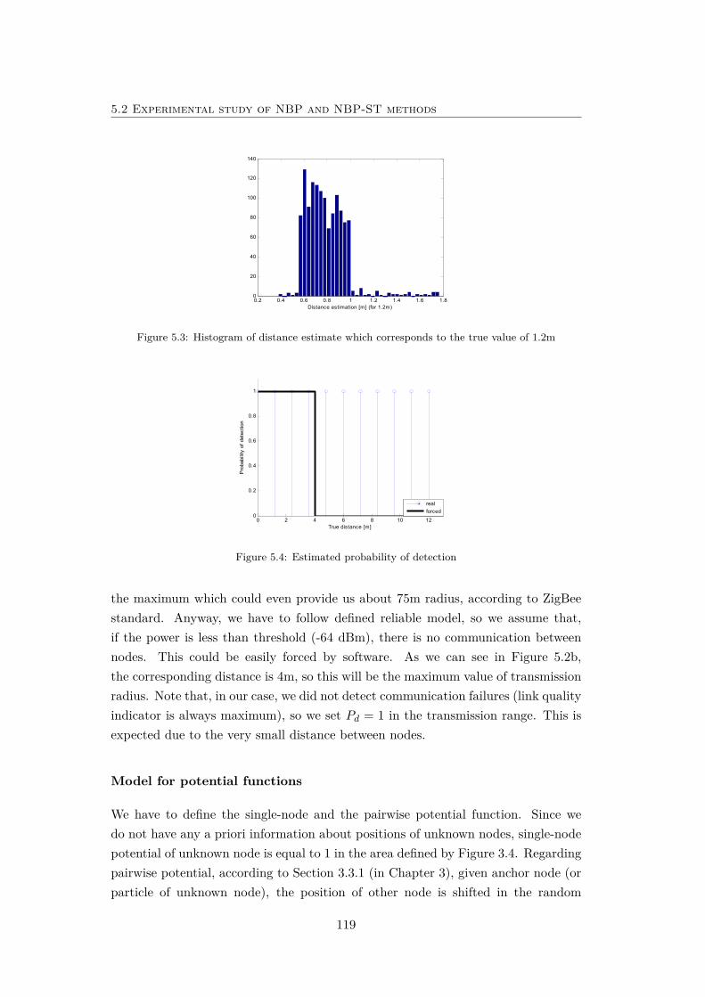
5.2 Experimental study of NBP and NBP-ST methods
0.2 0.4 0.6 0.8 1 1.2 1.4 1.6 1.80
20
40
60
80
100
120
140
Distance estimation [m] (for 1.2m)
Figure 5.3: Histogram of distance estimate which corresponds to the true value of 1.2m
0 2 4 6 8 10 120
0.2
0.4
0.6
0.8
1
True distance [m]
Pro
babi
lity
of d
etec
tion
realforced
Figure 5.4: Estimated probability of detection
the maximum which could even provide us about 75m radius, according to ZigBeestandard. Anyway, we have to follow defined reliable model, so we assume that,if the power is less than threshold (-64 dBm), there is no communication betweennodes. This could be easily forced by software. As we can see in Figure 5.2b,the corresponding distance is 4m, so this will be the maximum value of transmissionradius. Note that, in our case, we did not detect communication failures (link qualityindicator is always maximum), so we set Pd = 1 in the transmission range. This isexpected due to the very small distance between nodes.
Model for potential functions
We have to define the single-node and the pairwise potential function. Since wedo not have any a priori information about positions of unknown nodes, single-nodepotential of unknown node is equal to 1 in the area defined by Figure 3.4. Regardingpairwise potential, according to Section 3.3.1 (in Chapter 3), given anchor node (orparticle of unknown node), the position of other node is shifted in the random
119
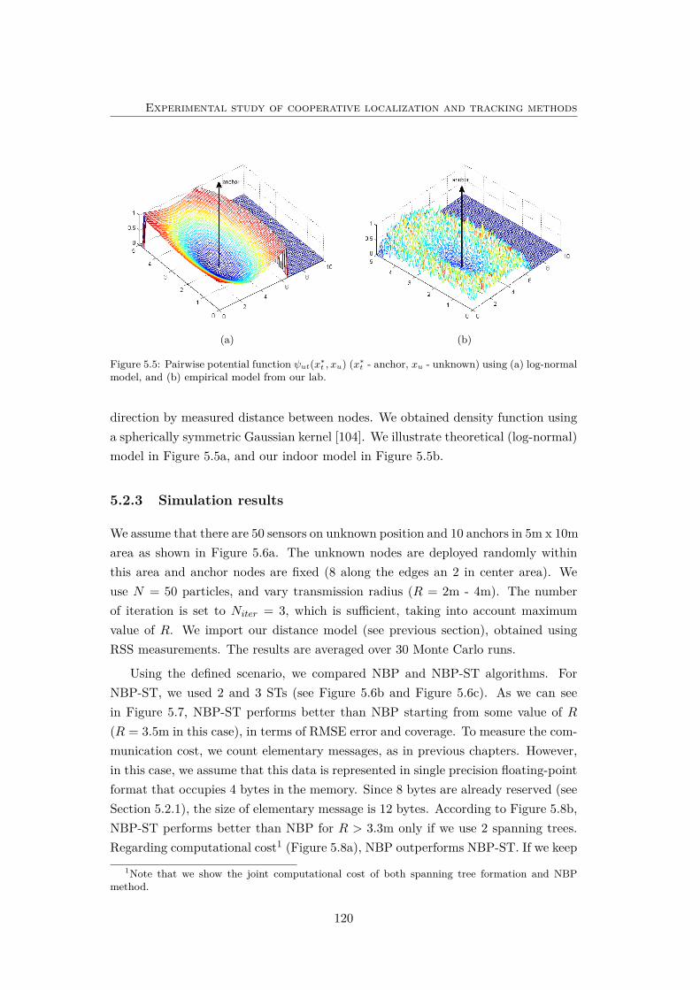
Experimental study of cooperative localization and tracking methods
(a) (b)
Figure 5.5: Pairwise potential function ψut(x∗t , xu) (x∗t - anchor, xu - unknown) using (a) log-normalmodel, and (b) empirical model from our lab.
direction by measured distance between nodes. We obtained density function usinga spherically symmetric Gaussian kernel [104]. We illustrate theoretical (log-normal)model in Figure 5.5a, and our indoor model in Figure 5.5b.
5.2.3 Simulation results
We assume that there are 50 sensors on unknown position and 10 anchors in 5m x 10marea as shown in Figure 5.6a. The unknown nodes are deployed randomly withinthis area and anchor nodes are fixed (8 along the edges an 2 in center area). Weuse N = 50 particles, and vary transmission radius (R = 2m - 4m). The numberof iteration is set to Niter = 3, which is sufficient, taking into account maximumvalue of R. We import our distance model (see previous section), obtained usingRSS measurements. The results are averaged over 30 Monte Carlo runs.
Using the defined scenario, we compared NBP and NBP-ST algorithms. ForNBP-ST, we used 2 and 3 STs (see Figure 5.6b and Figure 5.6c). As we can seein Figure 5.7, NBP-ST performs better than NBP starting from some value of R(R = 3.5m in this case), in terms of RMSE error and coverage. To measure the com-munication cost, we count elementary messages, as in previous chapters. However,in this case, we assume that this data is represented in single precision floating-pointformat that occupies 4 bytes in the memory. Since 8 bytes are already reserved (seeSection 5.2.1), the size of elementary message is 12 bytes. According to Figure 5.8b,NBP-ST performs better than NBP for R > 3.3m only if we use 2 spanning trees.Regarding computational cost1 (Figure 5.8a), NBP outperforms NBP-ST. If we keep
1Note that we show the joint computational cost of both spanning tree formation and NBPmethod.
120
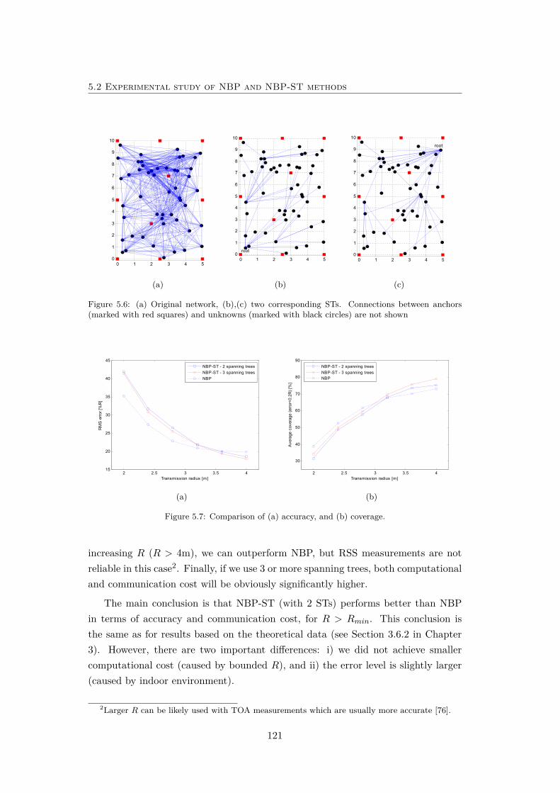
5.2 Experimental study of NBP and NBP-ST methods
0 1 2 3 4 50
1
2
3
4
5
6
7
8
9
10
(a)
0 1 2 3 4 50
1
2
3
4
5
6
7
8
9
10
root
(b)
0 1 2 3 4 50
1
2
3
4
5
6
7
8
9
10
root
(c)
Figure 5.6: (a) Original network, (b),(c) two corresponding STs. Connections between anchors(marked with red squares) and unknowns (marked with black circles) are not shown
2 2.5 3 3.5 415
20
25
30
35
40
45
Transmission radius [m]
RM
S e
rror [
%R
]
NBP-ST - 2 spanning treesNBP-ST - 3 spanning treesNBP
(a)
2 2.5 3 3.5 4
30
40
50
60
70
80
90
Transmission radius [m]
Ave
rage
cov
erag
e (e
rror<
0.2R
) [%
]
NBP-ST - 2 spanning treesNBP-ST - 3 spanning treesNBP
(b)
Figure 5.7: Comparison of (a) accuracy, and (b) coverage.
increasing R (R > 4m), we can outperform NBP, but RSS measurements are notreliable in this case2. Finally, if we use 3 or more spanning trees, both computationaland communication cost will be obviously significantly higher.
The main conclusion is that NBP-ST (with 2 STs) performs better than NBPin terms of accuracy and communication cost, for R > Rmin. This conclusion isthe same as for results based on the theoretical data (see Section 3.6.2 in Chapter3). However, there are two important differences: i) we did not achieve smallercomputational cost (caused by bounded R), and ii) the error level is slightly larger(caused by indoor environment).
2Larger R can be likely used with TOA measurements which are usually more accurate [76].
121
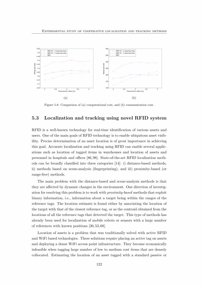
Experimental study of cooperative localization and tracking methods
2 2.5 3 3.5 40.05
0.1
0.15
0.2
0.25
0.3
0.35
0.4
0.45
0.5
0.55
Transmission radius [m]
MFl
ops
per n
ode
NBP-ST - 2 spanning treesNBP-ST - 3 spanning treesNBP
(a)
2 2.5 3 3.5 4100
150
200
250
300
350
400
Transmission radius [m]
Kby
tes
per n
ode
NBP-ST - 2 spanning treesNBP-ST - 3 spanning treesNBP
(b)
Figure 5.8: Comparison of (a) computational cost, and (b) communication cost.
5.3 Localization and tracking using novel RFID system
RFID is a well-known technology for real-time identification of various assets andusers. One of the main goals of RFID technology is to enable ubiquitous asset visib-ility. Precise determination of an asset location is of great importance in achievingthis goal. Accurate localization and tracking using RFID can enable several applic-ations such as location of tagged items in warehouses and location of assets andpersonnel in hospitals and offices [86, 98]. State-of-the-art RFID localization meth-ods can be broadly classified into three categories [14]: i) distance-based methods,ii) methods based on scene-analysis (fingerprinting), and iii) proximity-based (orrange-free) methods.
The main problem with the distance-based and scene-analysis methods is thatthey are affected by dynamic changes in the environment. One direction of investig-ation for resolving this problem is to work with proximity-based methods that exploitbinary information, i.e., information about a target being within the ranges of thereference tags. The location estimate is found either by associating the location ofthe target with that of the closest reference tag, or as the centroid obtained from thelocations of all the reference tags that detected the target. This type of methods hasalready been used for localization of mobile robots or sensors with a large numberof references with known positions [30,53,68].
Location of assets is a problem that was traditionally solved with active RFIDand WiFi based technologies. These solutions require placing an active tag on assetsand deploying a dense WiFi access point infrastructure. They become economicallyinfeasible when tagging large number of low to medium cost items that are denselycollocated. Estimating the location of an asset tagged with a standard passive or
122
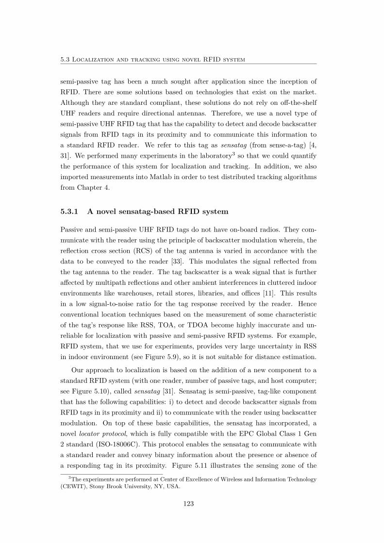
5.3 Localization and tracking using novel RFID system
semi-passive tag has been a much sought after application since the inception ofRFID. There are some solutions based on technologies that exist on the market.Although they are standard compliant, these solutions do not rely on off-the-shelfUHF readers and require directional antennas. Therefore, we use a novel type ofsemi-passive UHF RFID tag that has the capability to detect and decode backscattersignals from RFID tags in its proximity and to communicate this information toa standard RFID reader. We refer to this tag as sensatag (from sense-a-tag) [4,31]. We performed many experiments in the laboratory3 so that we could quantifythe performance of this system for localization and tracking. In addition, we alsoimported measurements into Matlab in order to test distributed tracking algorithmsfrom Chapter 4.
5.3.1 A novel sensatag-based RFID system
Passive and semi-passive UHF RFID tags do not have on-board radios. They com-municate with the reader using the principle of backscatter modulation wherein, thereflection cross section (RCS) of the tag antenna is varied in accordance with thedata to be conveyed to the reader [33]. This modulates the signal reflected fromthe tag antenna to the reader. The tag backscatter is a weak signal that is furtheraffected by multipath reflections and other ambient interferences in cluttered indoorenvironments like warehouses, retail stores, libraries, and offices [11]. This resultsin a low signal-to-noise ratio for the tag response received by the reader. Henceconventional location techniques based on the measurement of some characteristicof the tag’s response like RSS, TOA, or TDOA become highly inaccurate and un-reliable for localization with passive and semi-passive RFID systems. For example,RFID system, that we use for experiments, provides very large uncertainty in RSSin indoor environment (see Figure 5.9), so it is not suitable for distance estimation.
Our approach to localization is based on the addition of a new component to astandard RFID system (with one reader, number of passive tags, and host computer;see Figure 5.10), called sensatag [31]. Sensatag is semi-passive, tag-like componentthat has the following capabilities: i) to detect and decode backscatter signals fromRFID tags in its proximity and ii) to communicate with the reader using backscattermodulation. On top of these basic capabilities, the sensatag has incorporated, anovel locator protocol, which is fully compatible with the EPC Global Class 1 Gen2 standard (ISO-18006C). This protocol enables the sensatag to communicate witha standard reader and convey binary information about the presence or absence ofa responding tag in its proximity. Figure 5.11 illustrates the sensing zone of the
3The experiments are performed at Center of Excellence of Wireless and Information Technology(CEWIT), Stony Brook University, NY, USA.
123
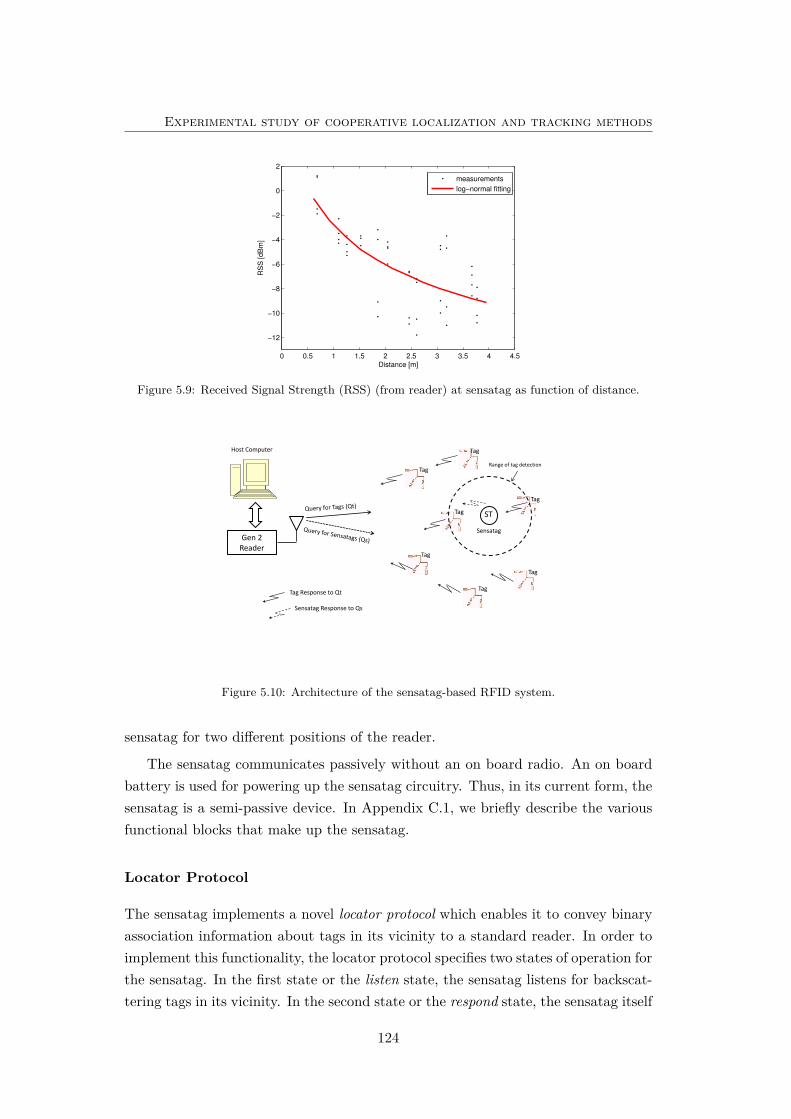
Experimental study of cooperative localization and tracking methods
0 0.5 1 1.5 2 2.5 3 3.5 4 4.5
−12
−10
−8
−6
−4
−2
0
2
Distance [m]
RS
S [
dB
m]
measurements
log−normal fitting
Figure 5.9: Received Signal Strength (RSS) (from reader) at sensatag as function of distance.
Gen 2 Reader
ST
Tag Response to Qt
Sensatag Response to Qs
Tag
Tag
Tag
Tag
Tag
Tag
Tag
Sensatag
Host Computer
Range of tag detection
Figure 5.10: Architecture of the sensatag-based RFID system.
sensatag for two different positions of the reader.
The sensatag communicates passively without an on board radio. An on boardbattery is used for powering up the sensatag circuitry. Thus, in its current form, thesensatag is a semi-passive device. In Appendix C.1, we briefly describe the variousfunctional blocks that make up the sensatag.
Locator Protocol
The sensatag implements a novel locator protocol which enables it to convey binaryassociation information about tags in its vicinity to a standard reader. In order toimplement this functionality, the locator protocol specifies two states of operation forthe sensatag. In the first state or the listen state, the sensatag listens for backscat-tering tags in its vicinity. In the second state or the respond state, the sensatag itself
124
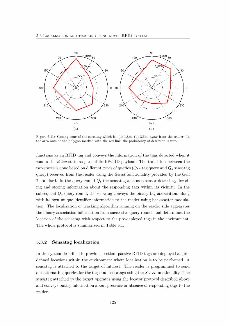
5.3 Localization and tracking using novel RFID system
50cm
100cm
150cm
30
210
60
240
90
270
120
300
150
330
180 0
(a)
50cm
100cm
150cm
30
210
60
240
90
270
120
300
150
330
180 0
(b)
Figure 5.11: Sensing zone of the sensatag which is: (a) 1.8m, (b) 3.6m, away from the reader. Inthe area outside the polygon marked with the red line, the probability of detection is zero.
functions as an RFID tag and conveys the information of the tags detected when itwas in the listen state as part of its EPC ID payload. The transition between thetwo states is done based on different types of queries (Qt - tag query and Qs sensatagquery) received from the reader using the Select functionality provided by the Gen2 standard. In the query round Qt the sensatag acts as a sensor detecting, decod-ing and storing information about the responding tags within its vicinity. In thesubsequent Qs query round, the sensatag conveys the binary tag association, alongwith its own unique identifier information to the reader using backscatter modula-tion. The localization or tracking algorithm running on the reader side aggregatesthe binary association information from successive query rounds and determines thelocation of the sensatag with respect to the pre-deployed tags in the environment.The whole protocol is summarized in Table 5.1.
5.3.2 Sensatag localization
In the system described in previous section, passive RFID tags are deployed at pre-defined locations within the environment where localization is to be performed. Asensatag is attached to the target of interest. The reader is programmed to sendout alternating queries for the tags and sensatags using the Select functionality. Thesensatag attached to the target operates using the locator protocol described aboveand conveys binary information about presence or absence of responding tags to thereader.
125
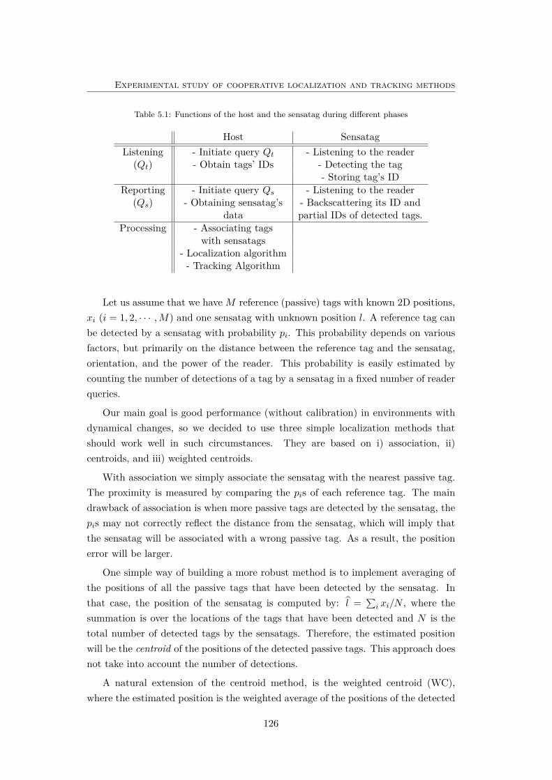
Experimental study of cooperative localization and tracking methods
Table 5.1: Functions of the host and the sensatag during different phases
Host SensatagListening - Initiate query Qt - Listening to the reader
(Qt) - Obtain tags’ IDs - Detecting the tag- Storing tag’s ID
Reporting - Initiate query Qs - Listening to the reader(Qs) - Obtaining sensatag’s - Backscattering its ID and
data partial IDs of detected tags.Processing - Associating tags
with sensatags- Localization algorithm- Tracking Algorithm
Let us assume that we haveM reference (passive) tags with known 2D positions,xi (i = 1, 2, · · · ,M) and one sensatag with unknown position l. A reference tag canbe detected by a sensatag with probability pi. This probability depends on variousfactors, but primarily on the distance between the reference tag and the sensatag,orientation, and the power of the reader. This probability is easily estimated bycounting the number of detections of a tag by a sensatag in a fixed number of readerqueries.
Our main goal is good performance (without calibration) in environments withdynamical changes, so we decided to use three simple localization methods thatshould work well in such circumstances. They are based on i) association, ii)centroids, and iii) weighted centroids.
With association we simply associate the sensatag with the nearest passive tag.The proximity is measured by comparing the pis of each reference tag. The maindrawback of association is when more passive tags are detected by the sensatag, thepis may not correctly reflect the distance from the sensatag, which will imply thatthe sensatag will be associated with a wrong passive tag. As a result, the positionerror will be larger.
One simple way of building a more robust method is to implement averaging ofthe positions of all the passive tags that have been detected by the sensatag. Inthat case, the position of the sensatag is computed by: l =
∑i xi/N , where the
summation is over the locations of the tags that have been detected and N is thetotal number of detected tags by the sensatags. Therefore, the estimated positionwill be the centroid of the positions of the detected passive tags. This approach doesnot take into account the number of detections.
A natural extension of the centroid method, is the weighted centroid (WC),where the estimated position is the weighted average of the positions of the detected
126
5.3 Localization and tracking using novel RFID system
tags. Since it is expected that the closer tags will be detected more times than moredistant ones, the weights are proportional to probabilities of detection of the tags.So, the estimated position is found as:
l =∑
ipixi =
∑i
N id
Nqxi (5.3)
where Nq is number of queries, and N id number of detections of a tag i by a sensatag.
A description of two potential applications (shelf identification and direction ofmovement estimation) is provided in Appendix C.2.
5.3.3 Sensatag tracking
Let us assume that we have K reference (passive) tags with known 2D positions, lk(k = 1, 2, · · · ,K) and one sensatag attached to an object with an unknown positionand velocity xt at time t. A reference tag can be detected by an sensatag withprobability pk,t. This probability depends on various factors, but primarily on thedistance between the reference tag and the sensatag, orientation, and the powerof the reader [11]. This probability is easily estimated by counting the number ofdetections of a tag by an sensatag in a fixed number of reader queries. Using thisobservation, our goal is to estimate xt at each time t.
We use the following discrete state-space model:
xt+1 = Axt +But (5.4)
yt = Cxt + vt (5.5)
where xt = [x1,t x2,t x1,t x2,t]T is the state vector at time t, which includes theposition and velocity of the sensatag that we want to estimate, ut = [u1,t u2,t]T isthe process noise (which accounts for the variation of the speed), yt = [y1,t y2,t]T isobservation at time t, and vt = [v1,t v2,t]T is observation noise. The observation isgiven as yt =
∑k pk,tlk, i.e., the weighted average of the positions of the detected
tags (i.e., WC method described above). This position estimate is more accurate(see next section) than other estimates found either by non-weighted average, orsimply by association with the nearest reference point. It is also worth noting that,since our observations represent static position estimates, our model is linear (incontrast to distance-based method, in Section 4.3.2). Given this observation, thesampling period TS , and assuming random motion of the target, we can define thematrices A, B, and C as follows:
127
Experimental study of cooperative localization and tracking methods
A =[
I 2 TSI 2
02 I 2
], B =
T 2S2 I 2
TSI 2
, C =[
I 2 02]
(5.6)
We apply the Bayesian approach to solve this tracking problem. filtering. Attime t, our goal is to estimate the posterior distribution p(xt|y1:t) given the priorp(xt−1|y1:t−1) (initially, p(x0|y0) = p(x0) is available), the state evolution p(xt|xt−1)(defined by the motion model (5.4)), and the likelihood function p(yt|xt) (defined bythe measurement model (5.5)). This posterior can be found by the prediction andfiltering equations [2] already used in Chapter 4 (equations (4.24), and (4.25)).
A standard closed-form solution can be found using traditional KF [116], assum-ing that the model is linear (as in our case), and that ut and vt are drawn fromGaussian distributions. The estimation of the process noise ut is generally very dif-ficult (it requires an accelerometer or a similar device attached to the target). Thus,we approximate ut by a Gaussian distribution. To make the process reliable, we needto find an upper bound of the true noise, e.g., by injecting enough uncertainty intothe covariance matrix. However, the measurement noise vt can be easily obtainedusing real samples. Generally, we cannot expect (especially, in indoor environment)that this noise vt is Gaussian, so KF is not an optimal solution for our problem.
Therefore, we apply the PF method [2] in which we represent the posterior PDFby a set of random samples (particles) with associated weights. We apply the well-known SIR method (called PF-SIR). In this method, the particles are drawn fromp(xt|xt−1), then weighted by the likelihood function, p(yt|xt), and finally, resampledin order to avoid the degeneracy problem (the situation in which all but one particlehave negligible weights). The PF-SIR method is summarized in Chapter 4 (Alg.11).
Note that in generally we don have a parametric form of likelihood function,so we can find its approximation using a KDE [104]. Namely, given a set of Ni
calibration samples vit = yit − Cxit, we have:
p(vt) =∑i
Kh(vt − vit) (5.7)
where Kh is the commonly used spherically symmetric Gaussian kernel: Kh(x) =N (x, 0, hI), and h is the bandwidth which controls the variance. To find h, we usethe generalized cross entropy estimator [13], which provides very accurate estimates.This kernel can be found offline prior to tracking. However, if the RFID systemis fast enough to provide Ni samples during the sampling period (TS) and also tocompute (5.7), the likelihood function can be obtained online, at each time frame.
128
5.3 Localization and tracking using novel RFID system
We can see that the main drawback of this method is high complexity. In thefollowing text, we propose PF with different model of the likelihood function.
Improved PF method (PF-BIN)
We propose a model for the number of detections of a tag by an sensatag and showhow we proceed with particle filtering. First, we model the probability of detectionof a tag by an sensatag according to
p = 11 + eα(d−d0) (5.8)
where d is the distance between a tag and the sensatag, and α > 0, d0 > 0 areparameters of the model, with d0 being the distance at which the probability ofdetection is equal to 1/2, and α being the parameter which determines the steepnessof the function.
Our measurements represent the number of times a tag is detected by an sensatagin N query rounds. We assume that during the N query rounds, the location ofthe object with the sensatag has not changed much (recall that the object with theattached sensatag is moving). Let the number of detections of the kth tag be equalto nk. Then the probability of nk is modeled by the binomial distribution, i.e.,
P (nk) =(N
nk
)pnkk (1− pk)N−nk (5.9)
where pk is given by (5.8) with d replaced by dk, the distance between the sensatagand the kth tag. In the field, there are total of K tags and for each of them we havea number of detections nk ∈ {0, 1, · · · , N}, k = 1, 2, · · · ,K.
Under the assumption that the parameters of the model in (5.8) are known (theyare estimated offline), we proceed with particle filtering as follows (note that we alsoassume that at time t− 1 we have the set of particles x(m)
t−1):
Step 1: Propagate the particles by using the prior, that is,
x(m)t ∼ p(xt|x(m)
t−1). (5.10)
Step 2: Compute the likelihood of the particles x(m)t given the measurements yt =
[n1,t n2,t · · ·nK,t]>. The likelihood function is given by
p(yt|x(m)t )
=∏Kk=1
(Nnk
)p
(m)nk,tk,t (1− p(m)
k,t )(N−nk,t) (5.11)
129
Experimental study of cooperative localization and tracking methods
where
p(m)k,t = 1
1 + eα(d(m)k,t−d0)
(5.12)
and d(m)k,t is the distance between the sensatag (whose location is defined by
the particle x(m)t ) and the k-th tag at time t. We note that the weights of the
particles are
w(m)t ∝ p(yt|x(m)
t ). (5.13)
Step 3: Resample with replacement.
We refer to this novel variant of PF-SIR, as PF-BIN method.
Distributed tracking
Current sensatag-based RFID system can only work in centralized fashion (i.e., thehost computer collects the data and runs the algorithms). However, with small modi-fications, sensatags can also perform the localization and the tracking algorithms indistributed way (recall that they are equipped with FPGA). It is only necessary toupdate sensatag software, and to provide appropriate protocol for communicationwith neighboring sensatags4. Note that, in contrast to the centralized case, thesensatags must be used as reference nodes (anchors).
Taking this into account, we can use the same model from the centralized scenariofor the simulation of the distributed tracking algorithms. Therefore, we can test theDPF methods (DPF-SBC, DPF-BG and DPF-BP) proposed in Section 4.3.2.
5.3.4 Experimental results
We now provide details of the experiments for studying sensatag-based RFID systemfor localization, tracking and related applications.
Sensatag localization
We deployed 12 passive tags in 6 reference points, where at each point we deployedtwo passive tags.5 The overall area was 1.6m x 1.3m. The setup is shown in Figure
4If we want to increase the communication range, they should be active as well (i.e., with on-board radio).
5The reason for having two passive tags at (nearly) same location was to prevent missing a tagby the sensatag because of eventual destructive superposition of the signals from the reader and the
130
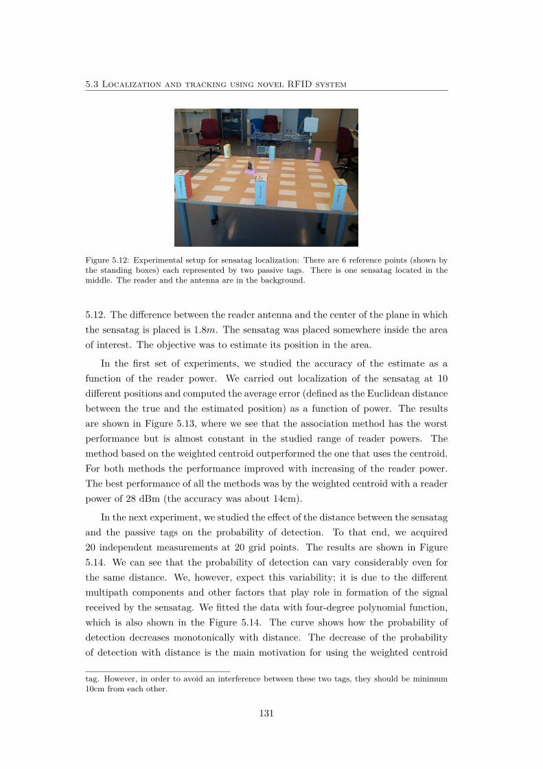
5.3 Localization and tracking using novel RFID system
Figure 5.12: Experimental setup for sensatag localization: There are 6 reference points (shown bythe standing boxes) each represented by two passive tags. There is one sensatag located in themiddle. The reader and the antenna are in the background.
5.12. The difference between the reader antenna and the center of the plane in whichthe sensatag is placed is 1.8m. The sensatag was placed somewhere inside the areaof interest. The objective was to estimate its position in the area.
In the first set of experiments, we studied the accuracy of the estimate as afunction of the reader power. We carried out localization of the sensatag at 10different positions and computed the average error (defined as the Euclidean distancebetween the true and the estimated position) as a function of power. The resultsare shown in Figure 5.13, where we see that the association method has the worstperformance but is almost constant in the studied range of reader powers. Themethod based on the weighted centroid outperformed the one that uses the centroid.For both methods the performance improved with increasing of the reader power.The best performance of all the methods was by the weighted centroid with a readerpower of 28 dBm (the accuracy was about 14cm).
In the next experiment, we studied the effect of the distance between the sensatagand the passive tags on the probability of detection. To that end, we acquired20 independent measurements at 20 grid points. The results are shown in Figure5.14. We can see that the probability of detection can vary considerably even forthe same distance. We, however, expect this variability; it is due to the differentmultipath components and other factors that play role in formation of the signalreceived by the sensatag. We fitted the data with four-degree polynomial function,which is also shown in the Figure 5.14. The curve shows how the probability ofdetection decreases monotonically with distance. The decrease of the probabilityof detection with distance is the main motivation for using the weighted centroid
tag. However, in order to avoid an interference between these two tags, they should be minimum10cm from each other.
131
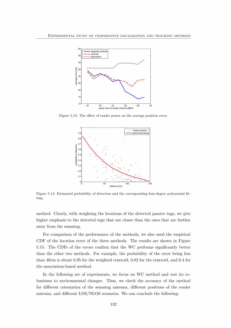
Experimental study of cooperative localization and tracking methods
20 22 24 26 28 3010
15
20
25
30
35
40
45
50
power level of reader antenna [dBm]
ave
rag
e e
rro
r [c
m]
weighted centroid
centroid
association
Figure 5.13: The effect of reader power on the average position error.
0 50 100 1500
0.1
0.2
0.3
0.4
0.5
0.6
0.7
0.8
0.9
1
distance [cm]
pro
ba
bili
ty o
f d
ete
ctio
n
measurements
polynomial fitting
Figure 5.14: Estimated probability of detection and the corresponding four-degree polynomial fit-ting.
method. Clearly, with weighting the locations of the detected passive tags, we givehigher emphasis to the detected tags that are closer than the ones that are furtheraway from the sensatag.
For comparison of the performance of the methods, we also used the empiricalCDF of the location error of the three methods. The results are shown in Figure5.15. The CDFs of the errors confirm that the WC performs significantly betterthan the other two methods. For example, the probability of the error being lessthan 40cm is about 0.95 for the weighted centroid, 0.82 for the centroid, and 0.4 forthe association-based method.
In the following set of experiments, we focus on WC method and test its ro-bustness to environmental changes. Thus, we check the accuracy of the methodfor different orientation of the sensatag antenna, different positions of the readerantenna, and different LOS/NLOS scenarios. We can conclude the following:
132
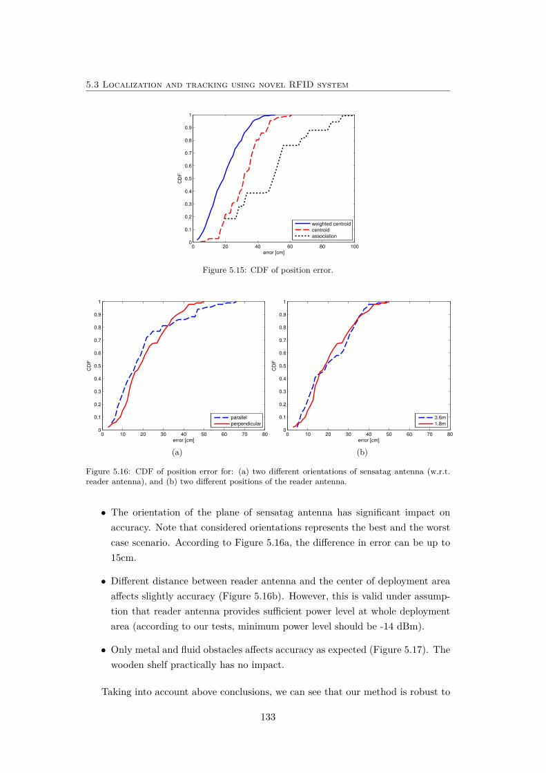
5.3 Localization and tracking using novel RFID system
0 20 40 60 80 1000
0.1
0.2
0.3
0.4
0.5
0.6
0.7
0.8
0.9
1
error [cm]
CD
F
weighted centroid
centroid
association
Figure 5.15: CDF of position error.
0 10 20 30 40 50 60 70 800
0.1
0.2
0.3
0.4
0.5
0.6
0.7
0.8
0.9
1
error [cm]
CD
F
parallel
perpendicular
(a)
0 10 20 30 40 50 60 70 800
0.1
0.2
0.3
0.4
0.5
0.6
0.7
0.8
0.9
1
error [cm]
CD
F
3.6m
1.8m
(b)
Figure 5.16: CDF of position error for: (a) two different orientations of sensatag antenna (w.r.t.reader antenna), and (b) two different positions of the reader antenna.
• The orientation of the plane of sensatag antenna has significant impact onaccuracy. Note that considered orientations represents the best and the worstcase scenario. According to Figure 5.16a, the difference in error can be up to15cm.
• Different distance between reader antenna and the center of deployment areaaffects slightly accuracy (Figure 5.16b). However, this is valid under assump-tion that reader antenna provides sufficient power level at whole deploymentarea (according to our tests, minimum power level should be -14 dBm).
• Only metal and fluid obstacles affects accuracy as expected (Figure 5.17). Thewooden shelf practically has no impact.
Taking into account above conclusions, we can see that our method is robust to
133
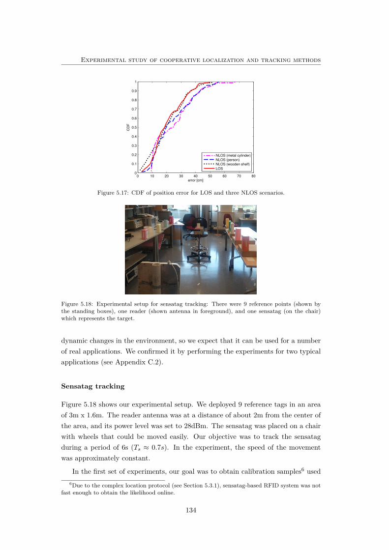
Experimental study of cooperative localization and tracking methods
0 10 20 30 40 50 60 70 800
0.1
0.2
0.3
0.4
0.5
0.6
0.7
0.8
0.9
1
error [cm]
CD
F
NLOS (metal cylinder)
NLOS (person)
NLOS (wooden shelf)
LOS
Figure 5.17: CDF of position error for LOS and three NLOS scenarios.
Figure 5.18: Experimental setup for sensatag tracking: There were 9 reference points (shown bythe standing boxes), one reader (shown antenna in foreground), and one sensatag (on the chair)which represents the target.
dynamic changes in the environment, so we expect that it can be used for a numberof real applications. We confirmed it by performing the experiments for two typicalapplications (see Appendix C.2).
Sensatag tracking
Figure 5.18 shows our experimental setup. We deployed 9 reference tags in an areaof 3m x 1.6m. The reader antenna was at a distance of about 2m from the center ofthe area, and its power level was set to 28dBm. The sensatag was placed on a chairwith wheels that could be moved easily. Our objective was to track the sensatagduring a period of 6s (Ts ≈ 0.7s). In the experiment, the speed of the movementwas approximately constant.
In the first set of experiments, our goal was to obtain calibration samples6 used6Due to the complex location protocol (see Section 5.3.1), sensatag-based RFID system was not
fast enough to obtain the likelihood online.
134
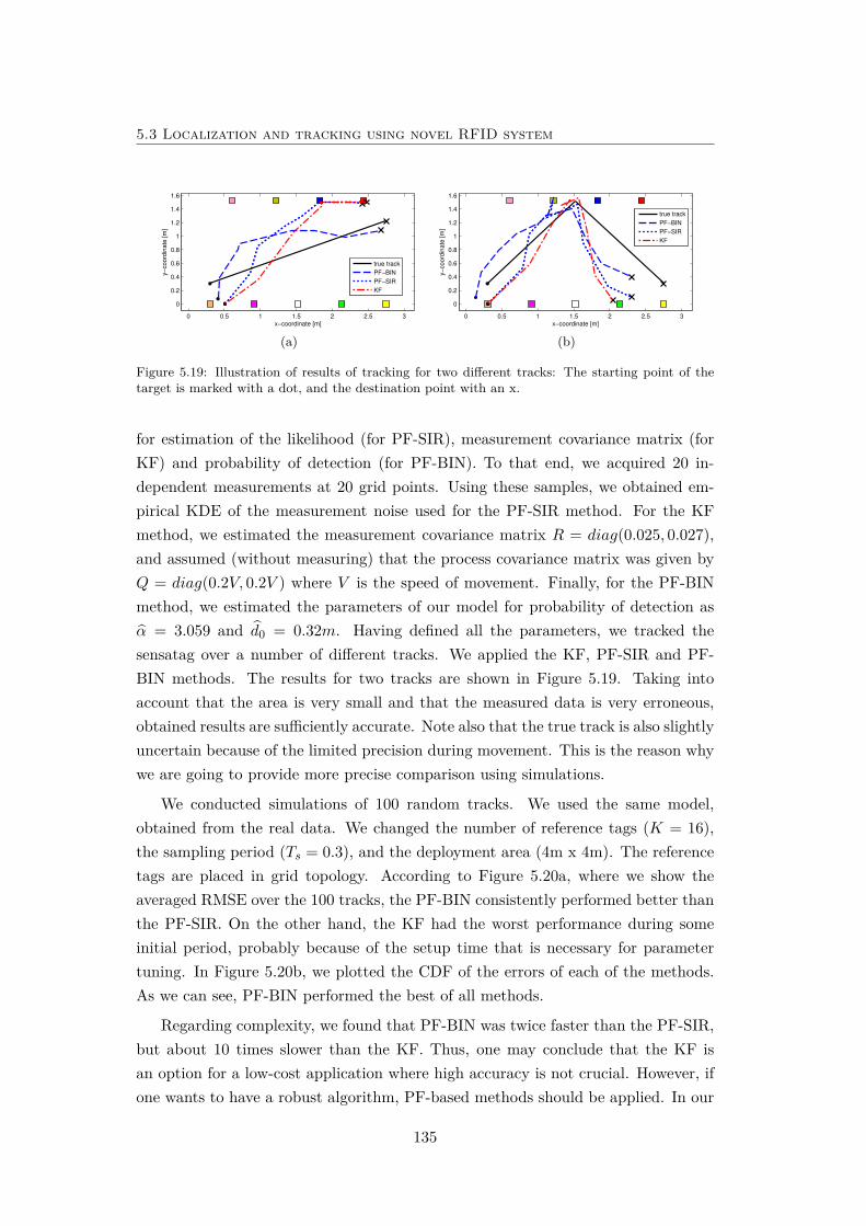
5.3 Localization and tracking using novel RFID system
0 0.5 1 1.5 2 2.5 3
0
0.2
0.4
0.6
0.8
1
1.2
1.4
1.6
x−coordinate [m]
y−
co
ord
ina
te [
m]
true track
PF−BIN
PF−SIR
KF
(a)
0 0.5 1 1.5 2 2.5 3
0
0.2
0.4
0.6
0.8
1
1.2
1.4
1.6
x−coordinate [m]
y−
co
ord
ina
te [
m]
true track
PF−BIN
PF−SIR
KF
(b)
Figure 5.19: Illustration of results of tracking for two different tracks: The starting point of thetarget is marked with a dot, and the destination point with an x.
for estimation of the likelihood (for PF-SIR), measurement covariance matrix (forKF) and probability of detection (for PF-BIN). To that end, we acquired 20 in-dependent measurements at 20 grid points. Using these samples, we obtained em-pirical KDE of the measurement noise used for the PF-SIR method. For the KFmethod, we estimated the measurement covariance matrix R = diag(0.025, 0.027),and assumed (without measuring) that the process covariance matrix was given byQ = diag(0.2V, 0.2V ) where V is the speed of movement. Finally, for the PF-BINmethod, we estimated the parameters of our model for probability of detection asα = 3.059 and d0 = 0.32m. Having defined all the parameters, we tracked thesensatag over a number of different tracks. We applied the KF, PF-SIR and PF-BIN methods. The results for two tracks are shown in Figure 5.19. Taking intoaccount that the area is very small and that the measured data is very erroneous,obtained results are sufficiently accurate. Note also that the true track is also slightlyuncertain because of the limited precision during movement. This is the reason whywe are going to provide more precise comparison using simulations.
We conducted simulations of 100 random tracks. We used the same model,obtained from the real data. We changed the number of reference tags (K = 16),the sampling period (Ts = 0.3), and the deployment area (4m x 4m). The referencetags are placed in grid topology. According to Figure 5.20a, where we show theaveraged RMSE over the 100 tracks, the PF-BIN consistently performed better thanthe PF-SIR. On the other hand, the KF had the worst performance during someinitial period, probably because of the setup time that is necessary for parametertuning. In Figure 5.20b, we plotted the CDF of the errors of each of the methods.As we can see, PF-BIN performed the best of all methods.
Regarding complexity, we found that PF-BIN was twice faster than the PF-SIR,but about 10 times slower than the KF. Thus, one may conclude that the KF isan option for a low-cost application where high accuracy is not crucial. However, ifone wants to have a robust algorithm, PF-based methods should be applied. In our
135
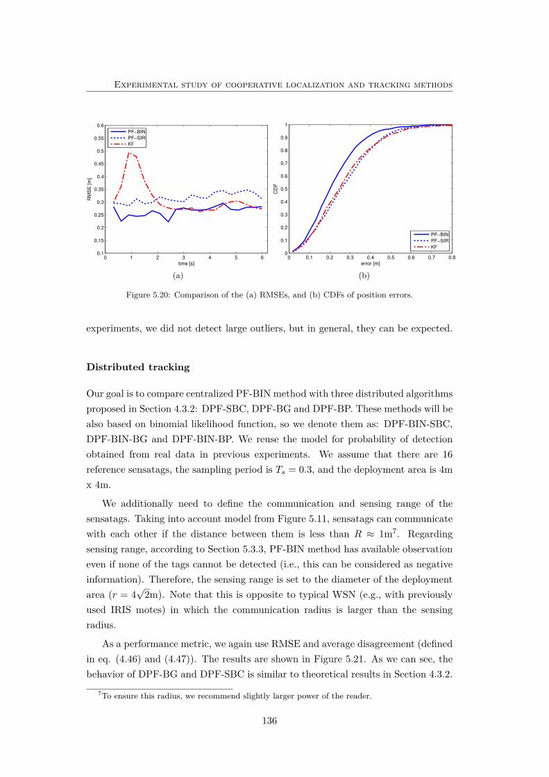
Experimental study of cooperative localization and tracking methods
0 1 2 3 4 5 60.1
0.15
0.2
0.25
0.3
0.35
0.4
0.45
0.5
0.55
0.6
time [s]
RM
SE
[m
]
PF−BIN
PF−SIR
KF
(a)
0 0.1 0.2 0.3 0.4 0.5 0.6 0.7 0.80
0.1
0.2
0.3
0.4
0.5
0.6
0.7
0.8
0.9
1
error [m]
CD
F
PF−BIN
PF−SIR
KF
(b)
Figure 5.20: Comparison of the (a) RMSEs, and (b) CDFs of position errors.
experiments, we did not detect large outliers, but in general, they can be expected.
Distributed tracking
Our goal is to compare centralized PF-BIN method with three distributed algorithmsproposed in Section 4.3.2: DPF-SBC, DPF-BG and DPF-BP. These methods will bealso based on binomial likelihood function, so we denote them as: DPF-BIN-SBC,DPF-BIN-BG and DPF-BIN-BP. We reuse the model for probability of detectionobtained from real data in previous experiments. We assume that there are 16reference sensatags, the sampling period is Ts = 0.3, and the deployment area is 4mx 4m.
We additionally need to define the communication and sensing range of thesensatags. Taking into account model from Figure 5.11, sensatags can communicatewith each other if the distance between them is less than R ≈ 1m7. Regardingsensing range, according to Section 5.3.3, PF-BIN method has available observationeven if none of the tags cannot be detected (i.e., this can be considered as negativeinformation). Therefore, the sensing range is set to the diameter of the deploymentarea (r = 4
√2m). Note that this is opposite to typical WSN (e.g., with previously
used IRIS motes) in which the communication radius is larger than the sensingradius.
As a performance metric, we again use RMSE and average disagreement (definedin eq. (4.46) and (4.47)). The results are shown in Figure 5.21. As we can see, thebehavior of DPF-BG and DPF-SBC is similar to theoretical results in Section 4.3.2.
7To ensure this radius, we recommend slightly larger power of the reader.
136
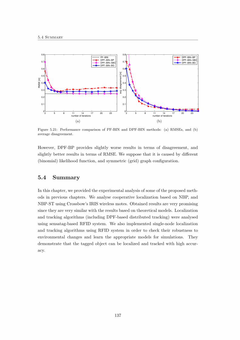
5.4 Summary
2 5 8 11 14 17 20 230
0.1
0.2
0.3
0.4
0.5
0.6
0.7
0.8
number of iterations
RM
SE
[m
]
PF−BIN
DPF−BIN−BP
DPF−BIN−SBC
DPF−BIN−BG
(a)
2 5 8 11 14 17 20 230
0.1
0.2
0.3
0.4
0.5
0.6
0.7
0.8
number of iterations
avg. dis
agre
em
ent [m
]
DPF−BIN−BP
DPF−BIN−SBC
DPF−BIN−BG
(b)
Figure 5.21: Performance comparison of PF-BIN and DPF-BIN methods: (a) RMSEs, and (b)average disagreement.
However, DPF-BP provides slightly worse results in terms of disagreement, andslightly better results in terms of RMSE. We suppose that it is caused by different(binomial) likelihood function, and symmetric (grid) graph configuration.
5.4 Summary
In this chapter, we provided the experimental analysis of some of the proposed meth-ods in previous chapters. We analyse cooperative localization based on NBP, andNBP-ST using Crossbow’s IRIS wireless motes. Obtained results are very promisingsince they are very similar with the results based on theoretical models. Localizationand tracking algorithms (including DPF-based distributed tracking) were analysedusing sensatag-based RFID system. We also implemented single-node localizationand tracking algorithms using RFID system in order to check their robustness toenvironmental changes and learn the appropriate models for simulations. Theydemonstrate that the tagged object can be localized and tracked with high accur-acy.
137

Experimental study of cooperative localization and tracking methods
138
Chapter 6
Conclusions and future work
6.1 Conslusions
We summarize below the main conclusions of this thesis:
• In Chapter 3, we proposed novel cooperative localization techniques basedon nonparametric message passing methods. The first contribution is NBBPmethod which is capable to archive better performance than NBP with lessparticles. Nevertheless, the main contributions of this chapters are four novelalgorithms for loopy networks: NGBP-JT, NGBP-PJT, NBP-ST, and URW-NBP. According to out results, we can conclude the following: i) NGBP-JTmethod, which provides accurate beliefs in loopy networks, has acceptablecomplexity only in small-scale sensor networks; i) NGBP-PJT can signific-antly outperform NBP, but it is not fully scalable, iii) NBP-ST can slightlyoutperform NBP method in highly-connected networks, and it is computation-ally feasible in large-scale ad-hoc/sensor networks; iv) URW-NBP is capable torun in asynchronous ad-hoc/sensor networks, and can slightly outperform NBPwhile keeping NBP’s robustness to failures. Although all proposed methodscan provide better estimates than NBP, our main conclusion is that URW-NBPleads to the best trade-off between accuracy, cost and robustness.
• In Chapter 4, we proposed novel algorithms for cooperative localization in mo-bile networks, and distributed target tracking. We extended NBP method forcooperative localization in mobile networks by providing: i) an optional 1-legsmoothing done almost in real-time, ii) a novel low-cost communication pro-tocol, and iii) more efficient sampling techniques. Moreover, novel algorithms,PMC-NBP and ANBP, which use more efficient sampling techniques, con-sistently outperform standard NBP. For the distributed target tracking, we
139
Conclusions and future work
proposed three DPF variants based on BC algorithms (DPF-SBC, DPF-BG,and DPF-BP). In contrast to previous methods, these methods can approx-imate global likelihood function in nonparametric form. According to ourresults, DPF-BG should be used in all tracking applications where minimalexpected error is crucial. On the other hand, if the agreement of the estimatesin the networks is more important than absolute error, DPF-BP could be agood choice. DPF-SBC, which guarantees convergence after large number ofiterations, could be applied when the cost and latency are not crucial.
• In Chapter 5, we provided the experimental analysis of NBP, NBP-ST andDPF methods. We used Crossbow’s IRIS wireless motes and novel semi-passiveRFID system. We also implemented single-node localization and tracking al-gorithms using RFID system in order to check their robustness to environ-mental changes and learn the appropriate models for simulations. Obtainedresults are very promising since they are very similar with the results basedon theoretical models.
6.2 Future work
Although we proposed a number of novel algorithms for cooperative localizationand tracking, by no means, the study in this thesis is complete. In this section,we propose several interesting topics for the future research. They can be dividedinto four categories: i) cooperative localization in static networks, ii) cooperativelocalization in mobile networks, iii) distributed target tracking, and iv) experimentalstudy of distributed algorithms.
Cooperative localization in static networks
One important remaining problem for the static networks is the case with non-rigid graphs, which usually appears in graphs with low connectivity. Although thisproblem was out of scope of this thesis, we know that bounded boxes and negativeinformation can be very helpful (e.g., see Figure 3.3). However, we expect thatadditional improvements are possible. For example, if NBP run in collaborativesubtrees (see Section 2.3.2), which are rigid, all the estimates will be unimodal.Then, postprocessing phase can take care of the nodes which are out of subtrees.Another interesting line of investigation could be additional improvements of theproposed algorithms in Chapter 3. Some tractable variant of TRW-NBP can bedeveloped, e.g., by computing the edge appearance probabilities using only localnode degree. Moreover, for GBP methods, it is eventually possible to find more
140
6.2 Future work
efficient approximations of the JT. Finally, some completely novel message-passingmethod can be developed, and compared with the proposed methods.
Cooperative localization in mobile networks
One line of investigation, in mobile networks, could be an additional improvementof the sampling techniques. For example, there is still question if it is possible toprovide NBP with linear complexity in the number of particles, while keeping thesimilar performance. Moreover, one can apply the NBP and variations for mobilelocalization with more informative mobility model. In that case, it might not benecessary to run NBP in each time frame, so the algorithm can keep running evenif NBP is relatively slow (comparing with sampling interval Ts). Regarding com-munication cost, one can find a different compression techniques for the packagesthat have to be transmitted. Finally, the security in sensor networks should be alsoinvestigated. The serious problems can happen in the whole network, if just onenode transmits completely wrong message (a set of particles), or if an anchor nodetransmits wrong coordinates. We expect that these problems can be partially solvedusing the ideas from the game theory.
Distributed target tracking
The remaining problem of fast DPF algorithms (DPF-BG and DPF-BP) is no guar-antee for the convergence to the true likelihood. DPF-BG provides the true likeli-hood only in expectation, and DPF-BP provides biased results in the networks withloops. One line of investigation could be a hybrid methods based on combination ofSBC, BG and BP, which might provide better convergence/performance trade-off.For example, the method which runs DPF-BP couple of iterations, then switchesto DPF-SBC, will likely inherit the fast convergence of DPF-BP and high accuracyof DPF-SBC. Moreover, DPF-BP can be also extended using ideas from Chapter 3.However, assuming that for this application, we prefer to avoid graph transformation(since for the mobile scenario we need low latency), DPF based on URW-BP couldbe a good option. Since all of the proposed algorithms are dedicated for single-targettracking (or tracking multiple targets which are well separated), one important lineof investigation is multi-target tracking in which we need to estimate both the stateand the label of the targets. Finally, distributed simultaneous localization and track-ing (SLAT) in WSN could be very challenging topic. For this problem, the resultsfrom Chapter 3 (NBP-based cooperative localization), and Chapter 4 (DPF-basedtarget tracking) can be combined.
141
Conclusions and future work
Experimental study of distributed algorithms
Although this thesis already includes several real experiments in indoor environment,the algorithms are always run on the host computer (i.e., in centralized fashion).Therefore, it would be interesting to see how proposed algorithms perform if run, oneach mote, in completely distributed way. Of course, we expect the similar accuracyas for already shown centralized emulations of distributed algorithms (in Chapter5). However, the latency is still unknown. Thus, the main question is what is theminimal sampling interval (Ts) within which NBP algorithms and variations can beexecuted. The latency of ST and JT formations, which cannot be run in parallel,should be also analysed. These transformations of the graph also require a robustand synchronized protocol. Finally, distributed implementation can more preciselyshow us the level of robustness of all algorithms.
142
Appendix A
GBP-JT: example network
In this appendix, we analyze GBP-JT for small-scale networks illustrated in FigureA.1. The network has 10 nodes, 5 anchors (nodes 6-10) and 5 unknowns (nodes 1-5).There is a loop 1-2-4-5-3, so we have to triangulate it by adding two more edges (2-3and 3-4). Then we define 8 cliques in the graph: C1 = {x1, x2, x3}, C2 = {x2, x3, x4},C3 = {x3, x4, x5}, C4 = {x4, x9} , C5 = {x5, x10}, C6 = {x1, x6}, C7 = {x2, x7},C8 = {x3, x8}. The appropriate potentials of the three-node cliques are given by:
ψC1(x1, x2, x3) = ψ12(x1, x2)ψ13(x1, x3)
ψC2(x2, x3, x4) = ψ24(x2, x4) (A.1)
ψC3(x3, x4, x5) = ψ35(x3, x5)ψ45(x4, x5)
where we, for simplicity, assumed that single-node potentials are uninformative.Note that “virtual” edges do not appear in these equations since they are used onlyto define cliques. Other cliques, defined over pairs of nodes, represent the potentialfunctions between two nodes (already known from standard BP):
ψC4(x4, x9) = ψ49(x4, x9), ψC5(x5, x10) = ψ510(x5, x10),
ψC6(x1, x6) = ψ16(x1, x6), ψC7(x2, x7) = ψ27(x2, x7), (A.2)
ψC8(x3, x8) = ψ38(x3, x8).
The junction tree corresponding to the network in Figure A.1 is shown in FigureA.2. As we can see, “anchor cliques” (C4 − C8) do not receive the messages, sothis graph does not contain loops. Actually, these “anchor cliques” also include oneunknown node so we can send them messages, but this node can be also located bymarginalizing the belief of some other clique.
143
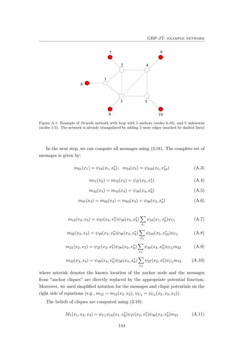
GBP-JT: example network
7 9
2 4
3 5
108
61
Figure A.1: Example of 10-node network with loop with 5 anchors (nodes 6-10), and 5 unknowns(nodes 1-5). The network is already triangulated by adding 2 more edges (marked by dashed lines)
In the next step, we can compute all messages using (3.18). The complete set ofmessages is given by:
m61(x1) = ψ16(x1, x∗6), m53(x5) = ψ510(x5, x
∗10) (A.3)
m71(x2) = m72(x2) = ψ27(x2, x∗7) (A.4)
m42(x4) = m43(x4) = ψ49(x4, x∗9) (A.5)
m81(x3) = m82(x3) = m83(x3) = ψ38(x3, x∗8) (A.6)
m12(x2, x3) = ψ27(x2, x∗7)ψ38(x3, x
∗8)∑x1
ψ16(x1, x∗6)ψC1 (A.7)
m32(x3, x4) = ψ49(x4, x∗9)ψ38(x3, x
∗8)∑x5
ψ510(x5, x∗10)ψC3 (A.8)
m21(x2, x3) = ψ27(x2, x∗7)ψ38(x3, x
∗8)∑x4
ψ49(x4, x∗9)ψC2m32 (A.9)
m23(x3, x4) = ψ49(x4, x∗9)ψ38(x3, x
∗8)∑x2
ψ27(x2, x∗7)ψC2m12 (A.10)
where asterisk denotes the known location of the anchor node and the messagesfrom “anchor cliques” are directly replaced by the appropriate potential function.Moreover, we used simplified notation for the messages and clique potentials on theright side of equations (e.g., m12 = m12(x2, x3), ψC2 = ψC2(x2, x3, x4)).
The beliefs of cliques are computed using (3.19):
M1(x1, x2, x3) = ψC1ψ16(x1, x∗6)ψ27(x2, x
∗7)ψ38(x3, x
∗8)m21 (A.11)
144
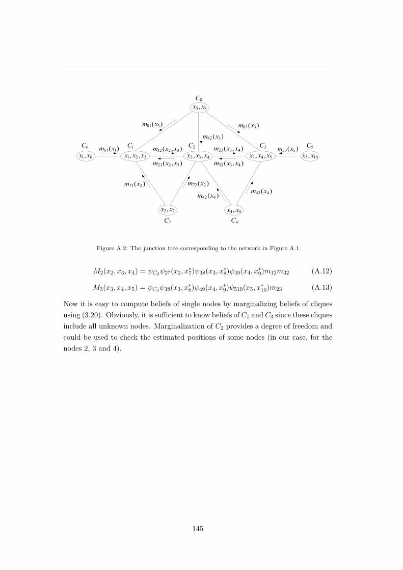
1 2 3, ,x x x12 2 3( , )m x x
2 3 4, ,x x x 3 4 5, ,x x x21 2 3( , )m x x
23 3 4( , )m x x
32 3 4( , )m x x1 6,x x
61 1( )m x5 10,x x
3 8,x x
2 7,x x 4 9,x x
83 3( )m x81 3( )m x
53 5( )m x
43 4( )m x71 2( )m x
82 3( )m x
42 4( )m x
72 2( )m x
8C
6C 1C 5C
7C 4C
2C 3C
Figure A.2: The junction tree corresponding to the network in Figure A.1
M2(x2, x3, x4) = ψC2ψ27(x2, x∗7)ψ38(x3, x
∗8)ψ49(x4, x
∗9)m12m32 (A.12)
M3(x3, x4, x5) = ψC3ψ38(x3, x∗8)ψ49(x4, x
∗9)ψ510(x5, x
∗10)m23 (A.13)
Now it is easy to compute beliefs of single nodes by marginalizing beliefs of cliquesusing (3.20). Obviously, it is sufficient to know beliefs of C1 and C3 since these cliquesinclude all unknown nodes. Marginalization of C2 provides a degree of freedom andcould be used to check the estimated positions of some nodes (in our case, for thenodes 2, 3 and 4).
145

GBP-JT: example network
146
Appendix B
Convergence behavior of BPconsensus
We analyse here the convergence behavior of BP consensus in loopy graphs. Itis already well-known [77] that BP consensus (as a special case of standard BP)converges to the exact solution after a finite number of iterations in cycle-free graphs.Using an appropriate message schedule, this number of iterations is equal to Dg + 1,where Dg is the diameter of the graph (i.e., the maximum hop-distance betweenany two nodes). However, for general graphs, it is straightforward to show (usingequation (4.40)) that the beliefs of BP consensus after Dg + 1 iterations is given by:
M (Dg+1)n (xt) ∝
∏u∈Gt
p(yu,t|xt)αu,n,t (B.1)
where αu,n,t ≥ 1 is an exponent (αu,n,t ∈ N) of node pair (u, n) at time t. In caseof cycle-free graphs αu,n,t = 1, so the estimated belief is equal to desired globallikelihood (given by (4.26)). In case of αu,t,n > 1, the observation from node u attime t is over-counted at node n. To understand the overcounting behavior, wedetermine αmax, the maximum value (maximized over n and u) of αu,n,t after Dg+1iterations. Note that running more than Dg + 1 iterations is unnecessary, as it willincrease the α-values. While for the general case this problem is hard, we limitourselves to some best- and the worst-case examples. In particular, we consider 4representative graph configurations, shown in Figure B.1:
1) Fully-connected graph (clique): For the example in Figure B.1a, Dg = 1, sothe belief at second iterations is given by (4.41). Since the graph is fully-connected,we know that the set Gn includes all nodes in the graph except node n (which islocally available). Therefore, αmax = 1, so BP consensus is correct.
147
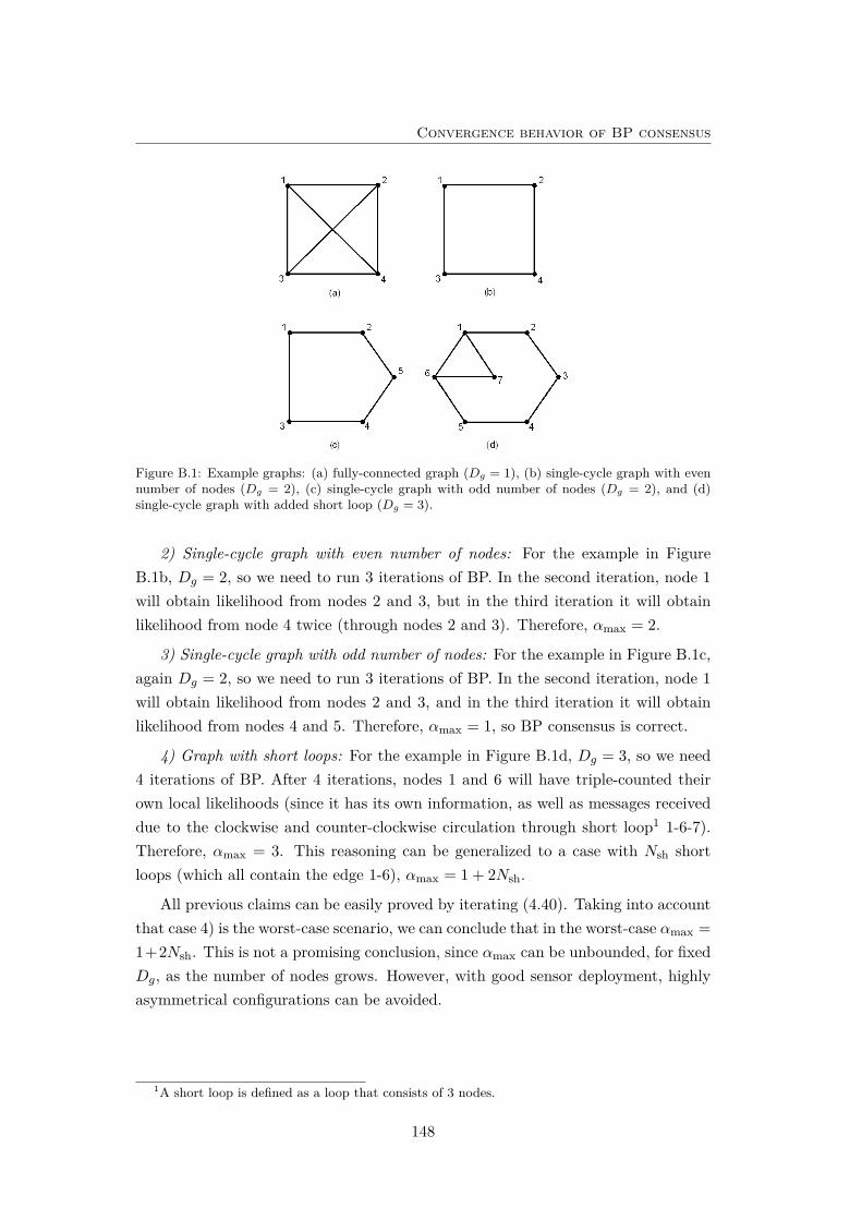
Convergence behavior of BP consensus
Figure B.1: Example graphs: (a) fully-connected graph (Dg = 1), (b) single-cycle graph with evennumber of nodes (Dg = 2), (c) single-cycle graph with odd number of nodes (Dg = 2), and (d)single-cycle graph with added short loop (Dg = 3).
2) Single-cycle graph with even number of nodes: For the example in FigureB.1b, Dg = 2, so we need to run 3 iterations of BP. In the second iteration, node 1will obtain likelihood from nodes 2 and 3, but in the third iteration it will obtainlikelihood from node 4 twice (through nodes 2 and 3). Therefore, αmax = 2.
3) Single-cycle graph with odd number of nodes: For the example in Figure B.1c,again Dg = 2, so we need to run 3 iterations of BP. In the second iteration, node 1will obtain likelihood from nodes 2 and 3, and in the third iteration it will obtainlikelihood from nodes 4 and 5. Therefore, αmax = 1, so BP consensus is correct.
4) Graph with short loops: For the example in Figure B.1d, Dg = 3, so we need4 iterations of BP. After 4 iterations, nodes 1 and 6 will have triple-counted theirown local likelihoods (since it has its own information, as well as messages receiveddue to the clockwise and counter-clockwise circulation through short loop1 1-6-7).Therefore, αmax = 3. This reasoning can be generalized to a case with Nsh shortloops (which all contain the edge 1-6), αmax = 1 + 2Nsh.
All previous claims can be easily proved by iterating (4.40). Taking into accountthat case 4) is the worst-case scenario, we can conclude that in the worst-case αmax =1+2Nsh. This is not a promising conclusion, since αmax can be unbounded, for fixedDg, as the number of nodes grows. However, with good sensor deployment, highlyasymmetrical configurations can be avoided.
1A short loop is defined as a loop that consists of 3 nodes.
148
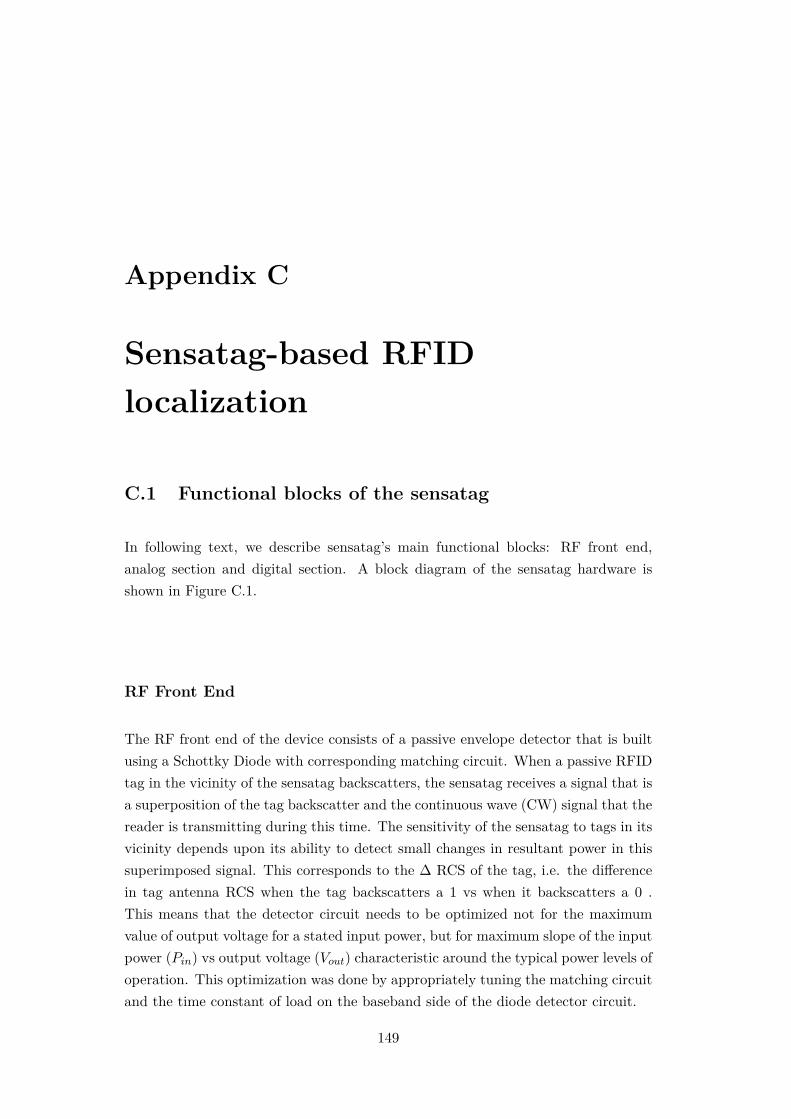
Appendix C
Sensatag-based RFIDlocalization
C.1 Functional blocks of the sensatag
In following text, we describe sensatag’s main functional blocks: RF front end,analog section and digital section. A block diagram of the sensatag hardware isshown in Figure C.1.
RF Front End
The RF front end of the device consists of a passive envelope detector that is builtusing a Schottky Diode with corresponding matching circuit. When a passive RFIDtag in the vicinity of the sensatag backscatters, the sensatag receives a signal that isa superposition of the tag backscatter and the continuous wave (CW) signal that thereader is transmitting during this time. The sensitivity of the sensatag to tags in itsvicinity depends upon its ability to detect small changes in resultant power in thissuperimposed signal. This corresponds to the ∆ RCS of the tag, i.e. the differencein tag antenna RCS when the tag backscatters a 1 vs when it backscatters a 0 .This means that the detector circuit needs to be optimized not for the maximumvalue of output voltage for a stated input power, but for maximum slope of the inputpower (Pin) vs output voltage (Vout) characteristic around the typical power levels ofoperation. This optimization was done by appropriately tuning the matching circuitand the time constant of load on the baseband side of the diode detector circuit.
149
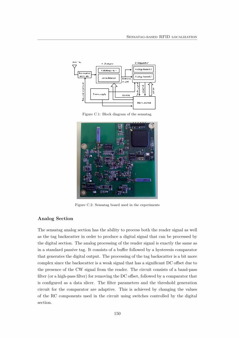
Sensatag-based RFID localization
Figure C.1: Block diagram of the sensatag.
Figure C.2: Sensatag board used in the experiments
Analog Section
The sensatag analog section has the ability to process both the reader signal as wellas the tag backscatter in order to produce a digital signal that can be processed bythe digital section. The analog processing of the reader signal is exactly the same asin a standard passive tag. It consists of a buffer followed by a hysteresis comparatorthat generates the digital output. The processing of the tag backscatter is a bit morecomplex since the backscatter is a weak signal that has a significant DC offset due tothe presence of the CW signal from the reader. The circuit consists of a band-passfilter (or a high-pass filter) for removing the DC offset, followed by a comparator thatis configured as a data slicer. The filter parameters and the threshold generationcircuit for the comparator are adaptive. This is achieved by changing the valuesof the RC components used in the circuit using switches controlled by the digitalsection.
150
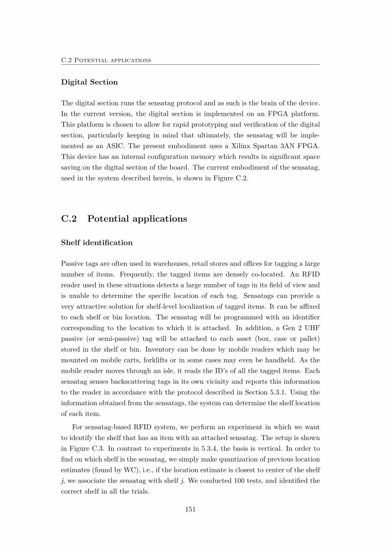
C.2 Potential applications
Digital Section
The digital section runs the sensatag protocol and as such is the brain of the device.In the current version, the digital section is implemented on an FPGA platform.This platform is chosen to allow for rapid prototyping and verification of the digitalsection, particularly keeping in mind that ultimately, the sensatag will be imple-mented as an ASIC. The present embodiment uses a Xilinx Spartan 3AN FPGA.This device has an internal configuration memory which results in significant spacesaving on the digital section of the board. The current embodiment of the sensatag,used in the system described herein, is shown in Figure C.2.
C.2 Potential applications
Shelf identification
Passive tags are often used in warehouses, retail stores and offices for tagging a largenumber of items. Frequently, the tagged items are densely co-located. An RFIDreader used in these situations detects a large number of tags in its field of view andis unable to determine the specific location of each tag. Sensatags can provide avery attractive solution for shelf-level localization of tagged items. It can be affixedto each shelf or bin location. The sensatag will be programmed with an identifiercorresponding to the location to which it is attached. In addition, a Gen 2 UHFpassive (or semi-passive) tag will be attached to each asset (box, case or pallet)stored in the shelf or bin. Inventory can be done by mobile readers which may bemounted on mobile carts, forklifts or in some cases may even be handheld. As themobile reader moves through an isle, it reads the ID’s of all the tagged items. Eachsensatag senses backscattering tags in its own vicinity and reports this informationto the reader in accordance with the protocol described in Section 5.3.1. Using theinformation obtained from the sensatags, the system can determine the shelf locationof each item.
For sensatag-based RFID system, we perform an experiment in which we wantto identify the shelf that has an item with an attached sensatag. The setup is shownin Figure C.3. In contrast to experiments in 5.3.4, the basis is vertical. In order tofind on which shelf is the sensatag, we simply make quantization of previous locationestimates (found by WC), i.e., if the location estimate is closest to center of the shelfj, we associate the sensatag with shelf j. We conducted 100 tests, and identified thecorrect shelf in all the trials.
151
Sensatag-based RFID localization
Figure C.3: Experimental setup for typical warehouse application: The goal is to find on whichshelf is sensatag.
Direction of movement (DOM) estimation
Accurate DOM estimation is crucial for many applications, in which we need to knowDOM of the person or object close to some monitoring area. Storage facilities ofteninventory their assets as the enter and leave the facility by installing RFID portalsat each entry/exit point. Conventional RFID systems suffer from two importantshortcomings: i) ambiguity in direction of asset motion (entering or exiting thefacility), and ii) cross reads between adjacent portals. These problems significantlyhamper the business intelligence derived from the deployed RFID system. Sensatagscan readily solve the above mentioned problems.
We describe here how to use location estimates for the DOM estimation. Thisproblem can be easily solved if we use 2 antennas, by measuring the times of detectionof the tagged object from the signals of the antennas [70]. However, due to the smallphysical distances of the whole setup, the more distant antenna from the incomingobject would read the tag almost at the same time as the nearer antenna, whichwould prevent easy determination of the DOM. Our solution for estimating theDOM of the sensatag relies on a reader with one antenna and on a number ofreference tags. In that case, DOM can be found by recognizing the pattern of thelocation samples (e.g., location estimates found by WC). One benefit of this method
152
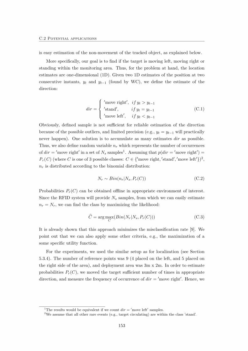
C.2 Potential applications
is easy estimation of the non-movement of the tracked object, as explained below.
More specifically, our goal is to find if the target is moving left, moving right orstanding within the monitoring area. Thus, for the problem at hand, the locationestimates are one-dimensional (1D). Given two 1D estimates of the position at twoconsecutive instants, yt and yt−1 (found by WC), we define the estimate of thedirection:
dir =
′move right′, if yt > yt−1′stand′, if yt = yt−1′move left′, if yt < yt−1
(C.1)
Obviously, defined sample is not sufficient for reliable estimation of the directionbecause of the possible outliers, and limited precision (e.g., yt = yt−1 will practicallynever happen). One solution is to accumulate as many estimates dir as possible.Thus, we also define random variable nr which represents the number of occurrencesof dir = ′move right′ in a set of Ns samples1. Assuming that p(dir = ′move right′) =Pr(C ) (where C is one of 3 possible classes: C ∈ {′move right, ′stand′, ′move left′})2,nr is distributed according to the binomial distribution:
Nr ∼ Bin(nr|Ns, Pr(C)) (C.2)
Probabilities Pr(C) can be obtained offline in appropriate environment of interest.Since the RFID system will provide Ns samples, from which we can easily estimatenr = Nr, we can find the class by maximizing the likelihood:
C = arg maxC
(Bin(Nr|Ns, Pr(C))) (C.3)
It is already shown that this approach minimizes the misclassification rate [9]. Wepoint out that we can also apply some other criteria, e.g., the maximization of asome specific utility function.
For the experiments, we used the similar setup as for localization (see Section5.3.4). The number of reference points was 9 (4 placed on the left, and 5 placed onthe right side of the area), and deployment area was 3m x 2m. In order to estimateprobabilities Pr(C), we moved the target sufficient number of times in appropriatedirection, and measure the frequency of occurrence of dir = ′move right′. Hence, we
1The results would be equivalent if we count dir = ′move left′ samples.2We assume that all other rare events (e.g., target circulating) are within the class ’stand’.
153
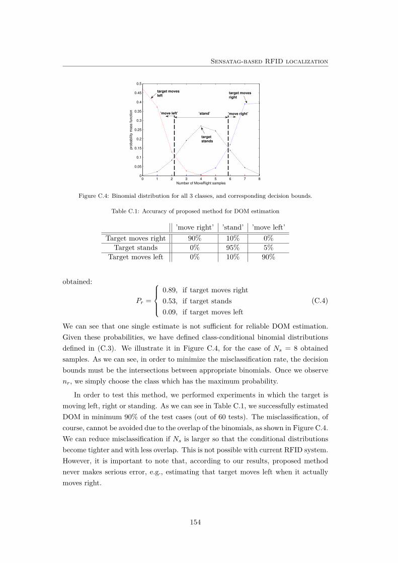
Sensatag-based RFID localization
0 1 2 3 4 5 6 7 80
0.05
0.1
0.15
0.2
0.25
0.3
0.35
0.4
0.45
0.5
Number of MoveRight samples
pro
ba
bili
ty m
ass f
un
ctio
n
’stand’’move left’ ’move right’
target movesleft
target movesright
targetstands
Figure C.4: Binomial distribution for all 3 classes, and corresponding decision bounds.
Table C.1: Accuracy of proposed method for DOM estimation
’move right’ ’stand’ ’move left’Target moves right 90% 10% 0%
Target stands 0% 95% 5%Target moves left 0% 10% 90%
obtained:
Pr =
0.89, if target moves right0.53, if target stands0.09, if target moves left
(C.4)
We can see that one single estimate is not sufficient for reliable DOM estimation.Given these probabilities, we have defined class-conditional binomial distributionsdefined in (C.3). We illustrate it in Figure C.4, for the case of Ns = 8 obtainedsamples. As we can see, in order to minimize the misclassification rate, the decisionbounds must be the intersections between appropriate binomials. Once we observenr, we simply choose the class which has the maximum probability.
In order to test this method, we performed experiments in which the target ismoving left, right or standing. As we can see in Table C.1, we successfully estimatedDOM in minimum 90% of the test cases (out of 60 tests). The misclassification, ofcourse, cannot be avoided due to the overlap of the binomials, as shown in Figure C.4.We can reduce misclassification if Ns is larger so that the conditional distributionsbecome tighter and with less overlap. This is not possible with current RFID system.However, it is important to note that, according to our results, proposed methodnever makes serious error, e.g., estimating that target moves left when it actuallymoves right.
154
Bibliography
[1] N. Ahmed, M. Rutten, T. Bessell, S. S. Kanhere, N. Gordon, and S. Jha,“Detection and tracking using particle-filter-based wireless sensor networks,”IEEE Transactions on Mobile Computing, vol. 9, no. 9, pp. 1332–1345, Sept.2010.
[2] M. S. Arulampalam, S. Maskell, N. G. Gordon, and T. Clapp, “A tutorial onparticle filters for online nonlinear/non-Gaussian Bayesian tracking,” IEEETransactions on Signal Processing, vol. 50, no. 2, pp. 174–188, Feb. 2002.
[3] AT86RF230, http://www.atmel.com/dyn/resources/prod_documents/doc5131.pdf.
[4] A. Athalye, V. Savic, M. Bolic, and P. M. Djuric, “A radio frequency identific-ation system for accurate indoor localization,” in Proc. of IEEE Int. Conf. onAcoustics, Speech and Signal Processing (ICASSP), May 2011, pp. 1777–1780.
[5] ATmega, http://www.atmel.com/dyn/resources/prod_documents/2549S.pdf.
[6] T. C. Aysal, M. E. Yildiz, A. D. Sarwate, and A. Scaglione, “Broadcast gossipalgorithms for consensus,” IEEE Transactions on Signal Processing, vol. 57,no. 7, pp. 2748–2761, 2009.
[7] D. A. Bader and K. Madduri, “Designing multithreaded algorithms forbreadth-first search and st-connectivity on the cray MTA-2,” in Proc. of Int.Conf. on Parallel Processing (ICPP), 2006, pp. 523–530.
[8] A. Baggio and K. Langendoen, “Monte Carlo localization for mobile wirelesssensor networks,” Ad Hoc Networks, vol. 6, no. 5, pp. 718–733, July 2008.
[9] C. M. Bishop, Pattern Recognition and Machine Learning. Secaucus, NJ,USA: Springer-Verlag New York, Inc., 2006.
155
BIBLIOGRAPHY
[10] M. Bolic, P. M. Djuric, and S. Hong, “Resampling algorithms and architec-tures for distributed particle filters,” IEEE Transactions on Signal Processing,vol. 53, no. 7, pp. 2442–2450, July 2005.
[11] M. Bolic, A. Athalye, and T. H. Li, Performance of Passive UHF RFID Sys-tems in Practice. John Wiley & Sons, Ltd, 2010, pp. 1–22.
[12] I. Borg and P. Groenen, Modern Multidimensional Scaling: Theory and Ap-plications. Springer, 2005.
[13] Z. I. Botev, “A novel nonparametric density estimator,” The University ofQueensland, Australia, Tech. Rep., 2006.
[14] M. Bouet and A. L. dos Santos, “RFID tags: Positioning principles and local-ization techniques,” in Proc. of Wireless Days, 2008, pp. 1–5.
[15] S. Boyd, A. Ghosh, B. Prabhakar, and D. Shah, “Randomized gossip al-gorithms,” IEEE Transactions on Information Theory, vol. 52, no. 6, pp.2508–2530, June 2006.
[16] M. Briers, A. Doucet, and S. S. Singh, “Sequential auxiliary particle beliefpropagation,” in Proc. of 8th Int. Conf. on Information Fusion, vol. 1, 2005.
[17] M. F. Bugallo, M. Hong, and P. M. Djuric, “Marginalized population MonteCarlo,” in Proc. of IEEE Int. Conf. on Acoustics, Speech and Signal Processing(ICASSP), 2009, pp. 2925–2928.
[18] T. Camp, J. Boleng, and V. Davies, “A survey of mobility models forad hoc network research,” Wireless Communications and Mobile Computing(WCMC), vol. 2, pp. 483–502, Sept. 2002.
[19] O. Cappe, A. Guillin, J.-M. Marin, C. P. Robert, and C. P. Roberty, “Popula-tion Monte Carlo,” Journal of Computational and Graphical Statistics, vol. 13,pp. 907–929, 2004.
[20] X. Chen, A. Edelstein, Y. Li, M. Coates, M. Rabbat, and A. Men, “SequentialMonte Carlo for simultaneous passive device-free tracking and sensor localiz-ation using received signal strength measurements,” in Proc. of IEEE/ACMInt. Conf. on Information Processing in Sensor Networks (IPSN), April 2011,pp. 342–353.
[21] C.-Y. Chong and S. P. Kumar, “Sensor networks: evolution, opportunities,and challenges,” Proc. of the IEEE, vol. 91, no. 8, pp. 1247–1256, Aug. 2003.
156
BIBLIOGRAPHY
[22] M. Coates, “Distributed particle filters for sensor networks,” in Proc. of 3rdWorkshop on Information Processing in Sensor Networks (IPSN), April 2004,pp. 99–107.
[23] J. Costa, N. Patwari, and A. O. Hero, III, “Distributed multidimensional scal-ing with adaptive weighting for node localization in sensor networks,” ACMTrans. on Sensor Networks, vol. -, pp. 1–26, June 2005.
[24] C. Crick and A. Pfeffer, “Loopy belief propagation as a basis for communic-ation in sensor networks,” in Uncertainty in Artificial Intelligence, 2003, pp.159–166.
[25] Crossbow, http://www.xbow.com.
[26] K. Das and H. Wymeersch, “Censored cooperative positioning for dense wire-less networks,” in Proc. of IEEE 21st Int. Symp. on Personal, Indoor andMobile Radio Communications (PIMRC), 2010, pp. 262–266.
[27] A. D. G. Dimakis, A. D. Sarwate, and M. J. Wainwright, “Geographic gos-sip: Efficient averaging for sensor networks,” IEEE Transactions on SignalProcessing, vol. 56, no. 3, pp. 1205–1216, March 2008.
[28] A. G. Dimakis, S. Kar, J. M. F. Moura, M. G. Rabbat, and A. Scaglione, “Gos-sip algorithms for distributed signal processing,” Proc. of the IEEE, vol. 98,no. 11, pp. 1847–1864, Nov. 2010.
[29] P. M. Djuric, J. Beaudeau, and M. Bugallo, “Non-centralized target trackingwith mobile agents,” in Proc. of IEEE Int. Conf. on Acoustics, Speech andSignal Processing (ICASSP), May 2011, pp. 5928–5931.
[30] P. M. Djuric, M. Vemula, and M. F. Bugallo, “Target tracking by particlefiltering in binary sensor networks,” IEEE Transactions on Signal Processing,vol. 56, no. 6, pp. 2229–2238, June 2008.
[31] P. Djuric and A. Athalye, “RFID system and method for localizing and track-ing a moving object with an rfid tag,” US Patent 11 799 257, 2010.
[32] P. Djuric, J. Kotecha, J. Zhang, Y. Huang, T. Ghirmai, M. Bugallo, andJ. Miguez, “Particle filtering,” IEEE Signal Processing Magazine, vol. 20, no. 5,pp. 19–38, Sept. 2003.
[33] D. M. Dobkin, The RF in RFID: Passive UHF RFID in Practice. Newton,MA, USA: Newnes, 2007.
157
BIBLIOGRAPHY
[34] N. I. Dopico, B. Bejar, S. V. Macua, P. Belanovic, and S. Zazo, “Improved an-imal tracking algorithms using distributed Kalman-based filters,” in EuropeanWireless Conference, 2011, pp. 1–8.
[35] A. Doucet and A. M. Johansen, “A tutorial on particle filtering and smoothing:fifteen years later,” The Oxford Handbook of Nonlinear Filtering, 2011.
[36] D. Fox, W. Burgard, F. Dellaert, and S. Thrun, “Monte Carlo localization:efficient position estimation for mobile robots,” in Proc. of the National Con-ference on Artificial Intelligence, Orlando, Florida, 1999.
[37] B. Frey and D. MacKay, “A revolution: Belief propagation in graphs withcycles,” in In Neural Information Processing Systems. MIT Press, 1998, pp.479–485.
[38] A. Galstyan, B. Krishnamachari, K. Lerman, and S. Pattem, “Distributedonline localization in sensor networks using a moving target,” in Proc. of 3rdInt. Symp. on Information Processing in Sensor Networks (IPSN), April 2004,pp. 61–70.
[39] A. F. Garcia-Fernandez and J. Grajal, “Multitarget tracking using the jointmultitrack probability density,” in Proc. of 12th Int. Conf. on InformationFusion, 2009, pp. 595–602.
[40] S. Gezici, Z. Tian, G. B. Giannakis, H. Kobayashi, A. F. Molisch, H. V. Poor,and Z. Sahinoglu, “Localization via ultra-wideband radios: a look at position-ing aspects for future sensor networks,” IEEE Signal Processing Magazine,vol. 22, no. 4, pp. 70–84, July 2005.
[41] D. Gu, “Distributed particle filter for target tracking,” in Proc. of IEEE Int.Conf. on Robotics and Automation (ICRA), April 2007, pp. 3856–3861.
[42] D. Gu, J. Sun, Z. Hu, and H. Li, “Consensus based distributed particle filterin sensor networks,” in Proc. of Int. Conf. Information and Automation, 2008,pp. 302–307.
[43] F. Gustafsson and F. Gunnarsson, “Mobile positioning using wireless networks:possibilities and fundamental limitations based on available wireless networkmeasurements,” IEEE Signal Processing Magazine, vol. 22, no. 4, pp. 41–53,July 2005.
[44] O. Hlinka, O. Sluciak, F. Hlawatsch, P. M. Djuric, and M. Rupp, “Distributedgaussian particle filtering using likelihood consensus,” in Proc. of IEEE Int.
158
BIBLIOGRAPHY
Conf. on Acoustics, Speech and Signal Processing (ICASSP), May 2011, pp.3756–3759.
[45] F. Hutter, B. Ng, and R. Dearden, “Incremental thin junction trees for dy-namic bayesian networks,” Darmstadt University of Technology, Tech. Rep.,2004.
[46] A. T. Ihler, J. W. I. Fisher, R. L. Moses, and A. S. Willsky, “Nonparametricbelief propagation for self-localization of sensor networks,” IEEE Journal onSelected Areas in Communications, vol. 23, no. 4, pp. 809–819, April 2005.
[47] A. T. Ihler, E. B. Sudderth, W. T. Freeman, and A. S. Willsky, “Efficientmultiscale sampling from products of Gaussian mixtures,” in Proc. of NeuralInformation Processing Systems (NIPS). Cambridge, MA: MIT Press, 2003.
[48] A. T. Ihler, “Inference in sensor networks: Graphical models and particlemethods,” Ph.D. dissertation, MIT, 2005.
[49] H. Jamali Rad, A. Amar, and G. Leus, “Cooperative mobile network localiza-tion via subspace tracking,” in Proc. of IEEE Int. Conf. on Acoustics, Speechand Signal Processing (ICASSP), May 2011, pp. 2612–2615.
[50] X. Ji and H. Zha, “Sensor positioning in wireless ad-hoc sensor networks usingmultidimensional scaling,” in Proc. of IEEE INFOCOM, vol. 4, 2004, pp.2652–2661.
[51] B. Jiang and B. Ravindran, “Completely distributed particle filters for targettracking in sensor networks,” in Proc. of IEEE Int. Parallel & DistributedProcessing Symp., 2011, pp. 334–344.
[52] M. Jordan and Y. Weiss, “Graphical models: probabilistic inference,” Hand-book of Neural Networks and Brain Theory. 2nd edition, vol. -, pp. 1–17, 2002.
[53] W. Kim, K. Mechitov, J.-Y. Choi, and S. Ham, “On target tracking with binaryproximity sensors,” in Proc. of 4th Int. Symp. on Information Processing inSensor Networks (IPSN), 2005, pp. 301–308.
[54] C. Knapp and G. Carter, “The generalized correlation method for estimation oftime delay,” IEEE Transactions on Acoustics, Speech, and Signal Processing,vol. 24, no. 4, pp. 320–327, 1976.
[55] D. Koller and N. Friedman, Probabilistic graphical models. MIT Press, 2009.
159
BIBLIOGRAPHY
[56] V. Kolmogorov, “Convergent tree-reweighted message passing for energy min-imization,” IEEE Transactions on Pattern Analysis and Machine Intelligence,vol. 28, no. 10, pp. 1568–1583, 2006.
[57] J. H. Kotecha and P. M. Djuric, “Gaussian sum particle filtering,” IEEE Trans-actions on Signal Processing, vol. 51, no. 10, pp. 2602–1612, Oct. 2003.
[58] C. M. Kreucher, “An information-based approach to sensor resource alloca-tion,” Ph.D. dissertation, The University of Michigan, 2005.
[59] K. Krishna and M. Narasimha Murty, “Genetic K-means algorithm,” IEEETransactions on Systems, Man, and Cybernetics, Part B: Cybernetics, vol. 29,no. 3, pp. 433–439, 1999.
[60] P. Krishnan, A. S. Krishnakumar, W.-H. Ju, C. Mallows, and S. N. Gamt,“A system for LEASE: location estimation assisted by stationary emitters forindoor rf wireless networks,” in Proc. of IEEE INFOCOM, vol. 2, 2004, pp.1001–1011.
[61] K. Langendoen and N. Reijers, “Distributed localization in wireless sensornetworks: a quantitative comparison,” Elsevier Computer Networks, vol. 43,no. 4, pp. 499–518, Nov. 2003.
[62] S. H. Lee and M. West, “Markov chain distributed particle filters (MCDPF),”in Proc. of 48th IEEE Conf. held jointly with the 2009 28th Chinese ControlConf Decision and Control (CDC/CCC), 2009, pp. 5496–5501.
[63] G. Mao, B. Fidan, and B. D. O. Anderson, “Wireless sensor network localiz-ation techniques,” Comput. Networks, vol. 51, no. 10, pp. 2529–2553, 2007.
[64] J. Miguez, “Analysis of parallelizable resampling algorithms for particle filter-ing,” Signal Processing, vol. 87, no. 12, pp. 3155 – 3174, 2007.
[65] A. J. Mooij, N. Goga, and W. Wesselink, “A distributed spanning tree al-gorithm for topology-aware networks,” in Proc. of the Conf. on Design, Ana-lysis, and Simulation of Distributed Systems, 2004.
[66] J. M. Mooij and H. J. Kappen, “Sufficient conditions for convergence of thesum–product algorithm,” IEEE Transactions on Information Theory, vol. 53,no. 12, pp. 4422–4437, Dec. 2007.
[67] L. M. Ni, Y. Liu, Y. C. Lau, and A. P. Patil, “LANDMARC: indoor locationsensing using active RFID,” in Proc. of 1st IEEE Int. Conf. on PervasiveComputing and Communications (PerCom), 2003, pp. 407–415.
160
BIBLIOGRAPHY
[68] D. Niculescu and B. Nath, “Ad hoc positioning system (APS),” in Proc. ofIEEE GLOBECOM, vol. 5, 2001, pp. 2926–2931.
[69] ——, “Ad hoc positioning system (APS) using AOA,” in Proc. of IEEE IN-FOCOM, vol. 3, Mar./Apr. 2003, pp. 1734–1743.
[70] Y. Oikawa, “Tag movement direction estimation methods in an RFID gatesystem,” in Proc. of 6th Int. Symp. on Wireless Communication Systems(ISWCS), 2009, pp. 41–45.
[71] A. Oka and L. Lampe, “Distributed target tracking using signal strength meas-urements by a wireless sensor network,” IEEE Journal on Selected Areas inCommunications, vol. 28, no. 7, pp. 1006–1015, Sept. 2010.
[72] R. Olfati-Saber and R. Murray, “Consensus problems in networks of agentswith switching topology and time-delays,” IEEE Transactions on AutomaticControl, vol. 49, no. 9, pp. 1520 – 1533, Sept. 2004.
[73] R. Olfati-Saber, E. Franco, E. Frazzoli, and J. S. Shamma, “Belief consensusand distributed hypothesis testing in sensor networks,” in Proc. of NESC Wor-skhop. Springer Verlag, 2006, pp. 169–182.
[74] B. N. Oreshkin and M. J. Coates, “Asynchronous distributed particle filtervia decentralized evaluation of gaussian products,” in Proc. of 13th Conf. onInformation Fusion (FUSION), 2010, pp. 1–8.
[75] B. W. Parkinson and J. J. Spilker, Global Positioning System: Theory &Applications (Volume One). Progress in Astronautics and Aeronautics, 1996.
[76] N. Patwari, J. N. Ash, S. Kyperountas, A. O. Hero, III, R. L. Moses, andN. S. Correal, “Locating the nodes: cooperative localization in wireless sensornetworks,” IEEE Signal Processing Magazine, vol. 22, no. 4, pp. 54–69, July2005.
[77] J. Pearl, Probabilistic Reasoning in Intelligent Systems: Networks of PlausibleInference. San Mateo: Morgan Kaufmann, 1988.
[78] R. Peng and M. L. Sichitiu, “Robust, probabilistic, constraint-based localiza-tion for wireless sensor networks,” in Proc. of 2nd IEEE Conf. on Sensor andAd Hoc Communications and Networks (SECON), 2005, pp. 541–550.
[79] F. Penna, H. Wymeersch, and V. Savic, “Uniformly reweighted belief propaga-tion for distributed bayesian hypothesis testing,” in Proc. of IEEE StatisticalSignal Processing Workshop (SSP), June 2011, pp. 733 –736.
161
BIBLIOGRAPHY
[80] T.-D. Pham, H. Q. Ngo, V.-D. Le, S. Lee, and Y.-K. Lee, “Broadcast gossipbased distributed hypothesis testing in wireless sensor networks,” in Proc. ofInt. Conf. on Advanced Technologies for Communications, 2009, pp. 84–87.
[81] M. K. Pitt and N. Shephard, “Filtering via simulation: Auxiliary particlefilters,” Journal of the American Statistical Association, vol. 94, no. 446, pp.590–599, June 1999.
[82] N. B. Priyantha, H. Balakrishnan, E. Demaine, and S. Teller, “Anchor-freedistributed localization in sensor networks,” MIT Laboratory for ComputerScience, Tech. Rep., 2003.
[83] T. S. Rappaport, J. H. Reed, and B. D. Woerner, “Position location usingwireless communications on highways of the future,” IEEE CommunicationsMagazine, vol. 34, no. 10, pp. 33–41, 1996.
[84] T. S. Rappaport, Wireless Communications: Principles and Practice. UpperSaddle River, NJ, USA: Prentice-Hall, Inc., 1995.
[85] K. Romer, “The lighthouse location system for smart dust,” in Proc. of the1st int. conf. on Mobile systems, applications and services, ser. MobiSys ’03,2003, pp. 15–30.
[86] T. Sanpechuda and L. Kovavisaruch, “A review of RFID localization: Ap-plications and techniques,” in Proc. of 5th Int. Conf. on Electrical Engineer-ing/Electronics, Computer, Telecommunications and Information Technology(ECTI-CON), vol. 2, may 2008, pp. 769 –772.
[87] V. Savic, A. Poblacion, S. Zazo, and M. Garcia, “An experimental study ofRSS-based indoor localization using nonparametric belief propagation basedon spanning trees,” in Proc. of 4th Int. Conf. on Sensor Technologies andApplications (SENSORCOMM), July 2010, pp. 238–243.
[88] ——, “Indoor positioning using nonparametric belief propagation based onspanning trees,” EURASIP Journal on Wireless Communications and Net-working, vol. 2010, pp. 1–12, Aug. 2010.
[89] V. Savic and S. Zazo, “Nonparametric boxed belief propagation for localizationin wireless sensor networks,” in Proc. of 3rd Int. Conf. on Sensor Technologiesand Applications (SENSORCOMM), 2009, pp. 520–525.
[90] ——, “Sensor localization using nonparametric generalized belief propagationin network with loops,” in Proc. of 12th Int. Conf. on Information Fusion,2009, pp. 1966–1973.
162
BIBLIOGRAPHY
[91] ——, “Nonparametric belief propagation based on spanning trees for cooper-ative localization in wireless sensor networks,” in Proc. IEEE 72nd VehicularTechnology Conf. Fall (VTC-Fall), Sept. 2010, pp. 1–5.
[92] ——, “Pseudo-junction tree method for cooperative localization in wirelesssensor networks,” in Proc. of 13th Int. Conf. on Information Fusion, July2010, pp. 1–8.
[93] ——, “Belief propagation techniques for cooperative localization in wirelesssensor networks,” in Handbook of Position Location: Theory, Practice, andAdvances (eds S. A. Zekavat and R. M. Buehrer), Wiley, 2011.
[94] V. Savic, A. Athalye, M. Bolic, and P. M. Djuric, “Particle filtering for indoorRFID tag tracking,” in Proc. of IEEE Statistical Signal Processing Workshop(SSP), June 2011, pp. 193 –196.
[95] V. Savic, H. Wymeersch, F. Penna, and S. Zazo, “Optimized edge appearanceprobability for cooperative localization based on tree-reweighted nonparamet-ric belief propagation,” in Proc. of IEEE Int. Conf. on Acoustics, Speech andSignal Processing (ICASSP), May 2011, pp. 3028–3031.
[96] V. Savic and S. Zazo, “Sensor localization using generalized belief propaga-tion in network with loops,” in Proc. of the 17th European Signal ProcessingConference (EUSIPCO), 2009.
[97] A. Savvides, H. Park, and M. B. Srivastava, “The bits and flops of the n-hopmultilateration primitive for node localization problems,” in Proc. of the 1stACM international workshop on Wireless sensor networks and applications.ACM, 2002, pp. 112–121.
[98] A. Sayed, A. Tarighat, and N. Khajehnouri, “Network-based wireless loca-tion: challenges faced in developing techniques for accurate wireless locationinformation,” IEEE Signal Processing Magazine, vol. 22, no. 4, pp. 24–40, July2005.
[99] J. Schiff, E. B. Sudderth, and K. Goldberg, “Nonparametric belief propagationfor distributed tracking of robot networks with noisy inter-distance measure-ments,” in Proc. of IEEE/RSJ Int. Conf. on Intelligent Robots and Systems,2009, pp. 1369–1376.
[100] Y. Shang, W. Rumi, Y. Zhang, and M. Fromherz, “Localization from con-nectivity in sensor networks,” IEEE Transactions on Parallel and DistributedSystems, vol. 15, no. 11, pp. 961–974, Nov. 2004.
163
BIBLIOGRAPHY
[101] Y. Shang and W. Ruml, “Improved MDS-based localization,” in Proc. of IEEEINFOCOM, vol. 4, 2004, pp. 2640–2651.
[102] Y. Shen, H. Wymeersch, and M. Z. Win, “Fundamental limits of widebandlocalization— part II: Cooperative networks,” IEEE Transactions on Inform-ation Theory, vol. 56, no. 10, pp. 4981–5000, 2010.
[103] X. Sheng, Y.-H. Hu, and P. Ramanathan, “Distributed particle filter withGMM approximation for multiple targets localization and tracking in wire-less sensor network,” in Proc. of Fourth Int. Symp. Information Processing inSensor Networks (IPSN), 2005, pp. 181–188.
[104] B. Silverman, Density Estimation for Statistics and Data Analysis. Chapmanand Hall, New York, 1986.
[105] E. B. Sudderth, A. T. Ihler, W. T. Freeman, and A. S. Willsky, “Nonparamet-ric belief propagation,” in Proc. of IEEE Int. Conf. on Computer Vision andPattern Recognition, vol. 1, 2003.
[106] D. Ustebay, M. Coates, and M. Rabbat, “Distributed auxiliary particle filtersusing selective gossip,” in Proc. of IEEE Int. Conf. on Acoustics, Speech andSignal Processing (ICASSP), May 2011, pp. 3296–3299.
[107] R. van der Merwe, A. Doucet, N. D. Freitas, and E. Wan, “The unscentedparticle filter,” in Proc. of Advances in Neural Information Processing Systems,Nov. 2001.
[108] M. Vemula, M. F. Bugallo, and P. M. Djuric, “Sensor self-localization withbeacon position uncertainty,” Signal Processing, vol. 89, pp. 1144–1154, June2009.
[109] V. Vivekanandan and V. W. S. Wong, “Concentric anchor beacon localiza-tion algorithm for wireless sensor networks,” IEEE Transactions on VehicularTechnology, vol. 56, no. 5, pp. 2733–2744, Sept. 2007.
[110] M. J. Wainwright, T. S. Jaakkola, and A. S. Willsky, “Tree-reweighted beliefpropagation algorithms and approximate ml estimation by pseudo-momentmatching,” in Proc. of AISTATS, 2003.
[111] M. Wainwright and M. Jordan, Graphical models, exponential families, andvariational inference. Now Publishers Inc., 2008.
[112] G. Wang and K. Yang, “A new approach to sensor node localization using RSSmeasurements in wireless sensor networks,” IEEE Transactions on WirelessCommunications, vol. 10, no. 5, pp. 1389–1395, May 2011.
164
BIBLIOGRAPHY
[113] X. Wang, X. Wang, and D. M. Wilkes, “A divide-and-conquer approach forminimum spanning tree-based clustering,” IEEE Transactions on Knowledgeand Data Engineering, vol. 21, no. 7, pp. 945–958, 2009.
[114] Y. Weiss, “Correctness of local probability propagation in graphical modelswith loops,” Neural Computation, vol. 12, pp. 1–41, 2000.
[115] Y. Weiss and W. T. Freeman, “Correctness of belief propagation in Gaussiangraphical models of arbitrary topology,” Neural Computation, vol. 13, pp.2173–2200, 2001.
[116] G. Welch and G. Bishop, “An introduction to the Kalman filter,” Universityof North Carolina at Chapel Hill, Tech. Rep., July 2006.
[117] J. L. Williams and R. A. Lau, “Data association by loopy belief propagation,”in Proc. of 13th Conf. on Information Fusion, July 2010, pp. 1–8.
[118] H. Wymeersch, J. Lien, and M. Z. Win, “Cooperative localization in wirelessnetworks,” Proc. of the IEEE, vol. 97, no. 2, pp. 427–450, 2009.
[119] H. Wymeersch, F. Penna, and V. Savic, “Uniformly reweighted belief propaga-tion for estimation and detection in wireless networks,” IEEE Transactions onWireless Communications, pp. 1–9, 2012.
[120] ——, “Uniformly reweighted belief propagation: A factor graph approach,” inProc. of IEEE Int. Symp. on Information Theory (ISIT), July 2011.
[121] J. S. Yedidia, W. T. Freeman, and Y. Weiss, Understanding belief propaga-tion and its generalizations. San Francisco, CA, USA: Morgan KaufmannPublishers Inc., 2003, pp. 239–269.
[122] J. Yi, S. Yang, and H. Cha, “Multi-hop-based Monte Carlo localization formobile sensor networks,” in Proc. of 4th IEEE Conf. on Sensor, Mesh and AdHoc Communications and Networks (SECON), 2007, pp. 162–171.
[123] A. Yoo, E. Chow, K. Henderson, W. McLendon, B. Hendrickson, and U. Cata-lyurek, “A scalable distributed parallel breadth-first search algorithm on blue-gene/L,” in Proc. ACM/IEEE SC 2005 Conf. Supercomputing, 2005.
[124] Y. Zhao, Y. Liu, and L. M. Ni, “VIRE: Active RFID-based localization usingvirtual reference elimination,” in Proc. of Int. Conf. on Parallel Processing(ICPP), 2007.
165
Related Documents


![Overview of Message Passing Algorithms for Cooperative ......Message passing Algorithm for Sensor Self-Localization in Wireless Networks”, ISIT 2011. [SLEEP] M. Welling and J.J.](https://static.cupdf.com/doc/110x72/5fa692baac944f1bc95544a2/overview-of-message-passing-algorithms-for-cooperative-message-passing-algorithm.jpg)