arXiv:1103.1492v1 [math.ST] 8 Mar 2011 The Annals of Statistics 2011, Vol. 39, No. 1, 232–260 DOI: 10.1214/10-AOS837 c Institute of Mathematical Statistics, 2011 NONPARAMETRIC ESTIMATION OF SURFACE INTEGRALS By Ra´ ul Jim´ enez 1 and J. E. Yukich 2 Universidad Carlos III de Madrid and Lehigh University The estimation of surface integrals on the boundary of an un- known body is a challenge for nonparametric methods in statistics, with powerful applications to physics and image analysis, among other fields. Provided that one can determine whether random shots hit the body, Cuevas et al. [Ann. Statist. 35 (2007) 1031–1051] es- timate the boundary measure (the boundary length for planar sets and the surface area for 3-dimensional objects) via the considera- tion of shots at a box containing the body. The statistics considered by these authors, as well as those in subsequent papers, are based on the estimation of Minkowski content and depend on a smoothing parameter which must be carefully chosen. For the same sampling scheme, we introduce a new approach which bypasses this issue, pro- viding strongly consistent estimators of both the boundary measure and the surface integrals of scalar functions, provided one can collect the function values at the sample points. Examples arise in experi- ments in which the density of the body can be measured by physical properties of the impacts, or in situations where such quantities as temperature and humidity are observed by randomly distributed sen- sors. Our method is based on random Delaunay triangulations and involves a simple procedure for surface reconstruction from a dense cloud of points inside and outside the body. We obtain basic asymp- totics of the estimator, perform simulations and discuss, via Google Earth’s data, an application to the image analysis of the Aral Sea coast and its cliffs. 1. Introduction. The estimation of functionals defined on the boundary Γ of an unknown body G ⊂ R d is a new branch of nonparametric statistics with powerful applications in several areas, including image analysis and stereology [9]. Cuevas et al. [8] address the estimation of the Minkowski Received November 2009; revised May 2010. 1 Supported in part by MEC Grant ECO-2008-05080 and CAM Grant 2008-00059-002. 2 Supported in part by NSF Grant DMS-08-05570. AMS 2000 subject classifications. Primary 62G05; secondary 60D05. Key words and phrases. Surface estimation, boundary measure, Delaunay triangula- tion, stabilization methods. This is an electronic reprint of the original article published by the Institute of Mathematical Statistics in The Annals of Statistics, 2011, Vol. 39, No. 1, 232–260. This reprint differs from the original in pagination and typographic detail. 1

Welcome message from author
This document is posted to help you gain knowledge. Please leave a comment to let me know what you think about it! Share it to your friends and learn new things together.
Transcript
arX
iv:1
103.
1492
v1 [
mat
h.ST
] 8
Mar
201
1
The Annals of Statistics
2011, Vol. 39, No. 1, 232–260DOI: 10.1214/10-AOS837c© Institute of Mathematical Statistics, 2011
NONPARAMETRIC ESTIMATION OF SURFACE INTEGRALS
By Raul Jimenez1 and J. E. Yukich2
Universidad Carlos III de Madrid and Lehigh University
The estimation of surface integrals on the boundary of an un-known body is a challenge for nonparametric methods in statistics,with powerful applications to physics and image analysis, amongother fields. Provided that one can determine whether random shotshit the body, Cuevas et al. [Ann. Statist. 35 (2007) 1031–1051] es-timate the boundary measure (the boundary length for planar setsand the surface area for 3-dimensional objects) via the considera-tion of shots at a box containing the body. The statistics consideredby these authors, as well as those in subsequent papers, are basedon the estimation of Minkowski content and depend on a smoothingparameter which must be carefully chosen. For the same samplingscheme, we introduce a new approach which bypasses this issue, pro-viding strongly consistent estimators of both the boundary measureand the surface integrals of scalar functions, provided one can collectthe function values at the sample points. Examples arise in experi-ments in which the density of the body can be measured by physicalproperties of the impacts, or in situations where such quantities astemperature and humidity are observed by randomly distributed sen-sors. Our method is based on random Delaunay triangulations andinvolves a simple procedure for surface reconstruction from a densecloud of points inside and outside the body. We obtain basic asymp-totics of the estimator, perform simulations and discuss, via GoogleEarth’s data, an application to the image analysis of the Aral Seacoast and its cliffs.
1. Introduction. The estimation of functionals defined on the boundaryΓ of an unknown body G⊂ R
d is a new branch of nonparametric statisticswith powerful applications in several areas, including image analysis andstereology [9]. Cuevas et al. [8] address the estimation of the Minkowski
Received November 2009; revised May 2010.1Supported in part by MEC Grant ECO-2008-05080 and CAM Grant 2008-00059-002.2Supported in part by NSF Grant DMS-08-05570.AMS 2000 subject classifications. Primary 62G05; secondary 60D05.Key words and phrases. Surface estimation, boundary measure, Delaunay triangula-
tion, stabilization methods.
This is an electronic reprint of the original article published by theInstitute of Mathematical Statistics in The Annals of Statistics,2011, Vol. 39, No. 1, 232–260. This reprint differs from the original in paginationand typographic detail.
1
2 R. JIMENEZ AND J. E. YUKICH
content
limε→0+
µ(⋃
x∈ΓBε(x))
2ε,(1.1)
µ := µd being the Lebesgue measure on Rd andBε(x) the closed d-dimensional
ball with center at x and radius ε. When the limit (1.1) exists, it is the mostbasic measure of the content of Γ and it coincides with length and surfacearea in dimensions 2 and 3, respectively [16]. Minkowski content estimatorsare based on random point samples distributed on a d-dimensional rect-angular solid containing G, for which one may determine whether a pointis in G or not. Roughly speaking, they are empirical measures of the ε-approximation
µ(⋃
x∈ΓBε(x))
2ε(1.2)
of the Minkowski content of Γ. Both the statistic considered by Cuevas etal. [8] and other closely related statistics [2, 10, 18] depend on the smoothingparameter ε, which must be chosen as a function of the size of the randompoint sample.
We propose a different nonparametric approach, free of smoothing param-eters, to estimate not only boundary lengths of planar sets and surface areasof solids, but also surface integrals of those scalar functions whose values areknowable at the sample points. While this paper focuses on instances wherethe body G is unknown, the proposed method is also of interest for bodieshaving a known but complex boundary, one having a surface integral defyingtraditional estimators.
The nonparametric estimation of surface integrals has practical applica-tions in image analysis, when the body G consists of some nonhomogeneousmaterial and the density h(x) of the material at x is collected at the sam-ple points. Thus, one might, for example, be interested in the mass perunit thickness of Γ, which corresponds to the surface integral commonlyrepresented by
∫
Γ hdΓ. In some instances, quantities such as temperatureand humidity can be measured by sensors randomly distributed on a set, inwhich an unknown body is embedded, and a fundamental problem is to es-timate the surface integral of these quantities on the boundary of the body.In other situations, including those arising in medical imaging, oncology andcardiology, knowledge of boundary length is of importance in the prognosisof an infarction, as well as in the assessment of the dissemination capacityof a tumor, as explained in Cuevas et al. [8].
Our statistics are based on the Delaunay triangulation of the samplepoints. Although the idea can be easily adapted to other graphs, in par-ticular to the Voronoi diagram, we chose the Delaunay triangulation for twospecific reasons:
ESTIMATION OF SURFACE INTEGRALS 3
1. It is a well-known tool in curve reconstruction methods. In particular,the β-skeleton [15], the Crust [1] and a wide range of related algorithmsinvolve computing Delaunay triangulations.
2. It is computationally efficient—for example, Boissonnat and Cazals [5]report a 3-dimensional Delaunay triangulation code which can handle500,000 randomly distributed points per minute.
The basic difference between previous methods and the one introducedhere is that formerly used methods estimate a fattened boundary, namely⋃
x∈ΓBε(x), whereas we directly estimate Γ by a surface (a curve if d= 2)properly selected among the polyhedra (polygons if d= 2) whose faces be-long to the Delaunay triangulation. Part of our methodology involves anew algorithm for surface reconstruction based on inner and outer samplingpoints, which differs substantially from the numerical methods for surfacereconstruction in which the sample points are on (or close to) the surfaceto be reconstructed. Our method is described in Section 2, where we intro-duce the relevant statistics. Section 3 establishes basic asymptotics of thesestatistics and provides a strongly consistent estimator of the surface inte-gral. In Section 4, we perform a simulation study. In particular, we estimatethe Minkowski content of sets, comparing our method with existing ones.An application to image analysis of the Aral Sea coast and its cliffs fromGoogle Earth’s data is discussed in Section 5. Section 6 summarizes ourconclusions. Our proofs, given in Section 7, rely on point process methods,including weak convergence of point processes and stabilization methods, atool for establishing general limit theorems for sums of weakly dependentterms in geometric probability [3, 19–21].
2. The method: Sewing boundaries of unknown sets. Following the basicassumptions of [8, 10], we will assume that G is a compact subset of an openand bounded d-dimensional rectangular solid Q and that the closure of theinterior of G has positive µ-measure. The boundary of G will be denoted byΓ, that is,
Γ := {x : for any ε > 0,Bε(x)∩G 6=∅ and Bε(x) ∩Gc 6=∅},
with Gc :=Q \G. It is assumed that the µ-boundary of G, defined by
{x : for any ε > 0, µ(Bε(x) ∩G)> 0 and µ(Bε(x)∩Gc)> 0},(2.1)
coincides with Γ. This rules out the existence of “extremities” to G havingnull d-dimensional Lebesgue measure. Thus, if we randomly plot enoughpoints in Q, there will be points inside and outside G close enough to anypoint on the boundary Γ. We assume that Γ is a (d−1)-rectifiable set. That
4 R. JIMENEZ AND J. E. YUKICH
is, there exists a countable collection of continuously differentiable mapsgi :R
d−1 →Rd such that
Hd−1
(
Γ∖
∞⋃
i=1
gi(Rd−1)
)
= 0,(2.2)
Hd−1 being the (d− 1)-dimensional Hausdorff measure [16]. We will assumethat Γ has finite Hausdorff measure and that Γ has tangent spaces whichare defined almost everywhere.
As in [8, 10], the sampling model consists of n i.i.d. random variablesX1, . . . ,Xn, uniformly distributed on Q, and n i.i.d. Bernoulli random vari-ables δ1, . . . , δn such that
δk =
{
1, if Xk ∈G,0, if Xk /∈G.
(2.3)
In other words, although G is unknown, we know whether a sample pointXk is inside G or not. In addition, given measurable h :Q→ R, we assumethat we know the values h(X1), . . . , h(Xn); in general, h is unknown on itsdomain, but we assume that we are able to collect its value at each of then sample points. Our goal is to estimate the surface integral of h, formallydefined by
∫
ΓhdΓ =
∫
Γh(γ)Hd−1(dγ).(2.4)
For sets Γ satisfying a stronger notion of (d− 1)-rectifiability, namely if Γis the Lipschitz image of a subset of R
d, the integral (2.4) coincides (upto a constant factor) with the Minkowski content of Γ when h = 1. Thusthe estimated target quantities in [2, 8, 10, 18] can be written as a surfaceintegral (2.4) with h(γ)≡ 1. This brings the issues and problems of [2, 8, 10,18] within the compass of this paper.
Denote by Xn the set of sample points {X1, . . . ,Xn} and let D(Xn) bethe Delaunay triangulation for Xn, namely the full collection of simplices(triangles when d= 2) with vertices in Xn satisfying the empty sphere cri-terion, namely that no point in Xn is inside the circumsphere (circumcircleif d = 2) of any simplex in D(Xn). For any sample of absolutely continu-ous i.i.d. points on R
d, there exists a unique Delaunay triangulation almostsurely [17]. Each simplex s ∈D(Xn) is represented by a subset of (d+1) ver-tices belonging to Xn, here denoted by {Xs(1), . . . ,Xs(d+1)}. Recalling (2.3),we introduce the sewing of Γ, denoted by S(Xn,Γ), and defined by
S(Xn,Γ) :=
{
s ∈D(Xn) : 1≤d+1∑
k=1
δs(k) ≤ d
}
.
ESTIMATION OF SURFACE INTEGRALS 5
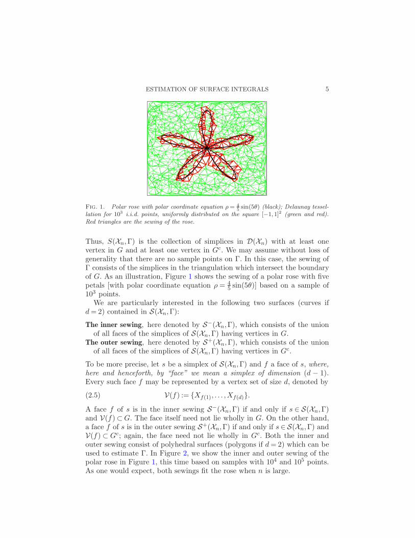
Fig. 1. Polar rose with polar coordinate equation ρ= 45sin(5θ) (black); Delaunay tessel-
lation for 103 i.i.d. points, uniformly distributed on the square [−1,1]2 (green and red).Red triangles are the sewing of the rose.
Thus, S(Xn,Γ) is the collection of simplices in D(Xn) with at least onevertex in G and at least one vertex in Gc. We may assume without loss ofgenerality that there are no sample points on Γ. In this case, the sewing ofΓ consists of the simplices in the triangulation which intersect the boundaryof G. As an illustration, Figure 1 shows the sewing of a polar rose with fivepetals [with polar coordinate equation ρ = 4
5 sin(5θ)] based on a sample of103 points.
We are particularly interested in the following two surfaces (curves ifd= 2) contained in S(Xn,Γ):
The inner sewing, here denoted by S−(Xn,Γ), which consists of the unionof all faces of the simplices of S(Xn,Γ) having vertices in G.
The outer sewing, here denoted by S+(Xn,Γ), which consists of the unionof all faces of the simplices of S(Xn,Γ) having vertices in Gc.
To be more precise, let s be a simplex of S(Xn,Γ) and f a face of s, where,here and henceforth, by “face” we mean a simplex of dimension (d − 1).Every such face f may be represented by a vertex set of size d, denoted by
V(f) := {Xf(1), . . . ,Xf(d)}.(2.5)
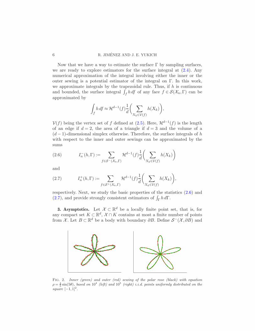
A face f of s is in the inner sewing S−(Xn,Γ) if and only if s ∈ S(Xn,Γ)and V(f)⊂G. The face itself need not lie wholly in G. On the other hand,a face f of s is in the outer sewing S+(Xn,Γ) if and only if s ∈ S(Xn,Γ) andV(f) ⊂ Gc; again, the face need not lie wholly in Gc. Both the inner andouter sewing consist of polyhedral surfaces (polygons if d= 2) which can beused to estimate Γ. In Figure 2, we show the inner and outer sewing of thepolar rose in Figure 1, this time based on samples with 104 and 105 points.As one would expect, both sewings fit the rose when n is large.
6 R. JIMENEZ AND J. E. YUKICH
Now that we have a way to estimate the surface Γ by sampling surfaces,we are ready to explore estimators for the surface integral at (2.4). Anynumerical approximation of the integral involving either the inner or theouter sewing is a potential estimator of the integral on Γ. In this work,we approximate integrals by the trapezoidal rule. Thus, if h is continuousand bounded, the surface integral
∫
f hdf of any face f ∈ S(Xn,Γ) can be
approximated by∫
fhdf ≈Hd−1(f)
1
d
(
∑
Xk∈V(f)
h(Xk)
)
,
V(f) being the vertex set of f defined at (2.5). Here, Hd−1(f) is the lengthof an edge if d = 2, the area of a triangle if d = 3 and the volume of a(d− 1)-dimensional simplex otherwise. Therefore, the surface integrals of hwith respect to the inner and outer sewings can be approximated by thesums
I−n (h,Γ) :=∑
f∈S−(Xn,Γ)
Hd−1(f)1
d
(
∑
Xk∈V(f)
h(Xk)
)
(2.6)
and
I+n (h,Γ) :=∑
f∈S+(Xn,Γ)
Hd−1(f)1
d
(
∑
Xk∈V(f)
h(Xk)
)
,(2.7)
respectively. Next, we study the basic properties of the statistics (2.6) and(2.7), and provide strongly consistent estimators of
∫
Γ hdΓ.
3. Asymptotics. Let X ⊂ Rd be a locally finite point set, that is, for
any compact set K ⊂Rd, X ∩K contains at most a finite number of points
from X . Let B ⊂ Rd be a body with boundary ∂B. Define S−(X , ∂B) and
Fig. 2. Inner (green) and outer (red) sewing of the polar rose (black) with equationρ= 4
5sin(5θ), based on 104 (left) and 105 (right) i.i.d. points uniformly distributed on the
square [−1,1]2.
ESTIMATION OF SURFACE INTEGRALS 7
S+(X , ∂B) analogously to S−(Xn,Γ) and S+(Xn,Γ), respectively. For x ∈X , when x ∈ S−(X , ∂B), we let ξ−(x,X ,B) be the normalized sum of theHausdorff measures of the faces belonging to S−(X , ∂B) and containing x.If x /∈ S−(X , ∂B), then we put ξ−(x,X ,B) = 0. Thus,
ξ−(x,X ,B) :=
1
d
∑
{f∈S−(X ,∂B) : x∈V(f)}
Hd−1(f), if x ∈⋃
f∈S−(X ,∂B)
V(f),
0, otherwise.
Similarly, we define ξ+(x,X ,B) to be the normalized sum of the Hausdorffmeasures of the faces belonging to S+(X , ∂B) and containing x; if no suchface exists, then ξ+ is defined to be zero.
We will use the functionals ξ− and ξ+ for several purposes; in particular,the statistics (2.6) and (2.7) can be expressed as the weighted sums
I−n (h,Γ) =
n∑
k=1
h(Xk)ξ−(Xk,Xn,G)(3.1)
and
I+n (h,Γ) =n∑
k=1
h(Xk)ξ+(Xk,Xn,G).(3.2)
The functional ξ− is translation invariant, that is, for all x ∈Rd, all locally
finite X and all bodies B, we have ξ−(x,X ,B) = ξ−(0,X − x,B − x); here,0 is a point at the origin of Rd and for sets F ⊂ R
d and x ∈ Rd, we put
{F −x} := {y−x :y ∈ F}. Also, given α > 0 and putting αF := {αy :y ∈ F},we have Hd−1(αf) = αd−1Hd−1(f). Thus, ξ− satisfies the following scalingproperty for all η > 0:
ηd−1ξ−(0,X ,B) = ξ−(0, ηX , ηB),(3.3)
which, when combined with translation invariance, gives
ηd−1ξ−(x,X ,B) = ξ−(0, η(X − x), η(B − x)).(3.4)
Thus, by the definition of I−n (h,Γ), we have
I−n (h,Γ) = n−(d−1)/dn∑
k=1
h(Xk)ξ−(0, n1/d(Xn −Xk), n
1/d(G−Xk)).(3.5)
Similarly, ξ+ is translation invariant and satisfies the scaling property (3.4)and, therefore,
I+n (h,Γ) = n−(d−1)/dn∑
k=1
h(Xk)ξ+(0, n1/d(Xn −Xk), n
1/d(G−Xk)).(3.6)
8 R. JIMENEZ AND J. E. YUKICH
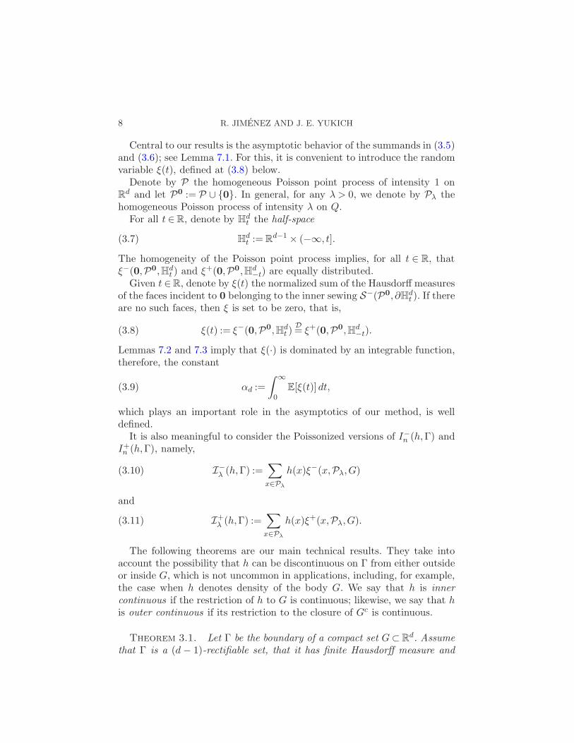
Central to our results is the asymptotic behavior of the summands in (3.5)and (3.6); see Lemma 7.1. For this, it is convenient to introduce the randomvariable ξ(t), defined at (3.8) below.
Denote by P the homogeneous Poisson point process of intensity 1 onRd and let P0 := P ∪ {0}. In general, for any λ > 0, we denote by Pλ the
homogeneous Poisson process of intensity λ on Q.For all t ∈R, denote by H
dt the half-space
Hdt :=R
d−1 × (−∞, t].(3.7)
The homogeneity of the Poisson point process implies, for all t ∈ R, thatξ−(0,P0,Hd
t ) and ξ+(0,P0,Hd−t) are equally distributed.
Given t ∈R, denote by ξ(t) the normalized sum of the Hausdorff measuresof the faces incident to 0 belonging to the inner sewing S−(P0, ∂Hd
t ). If thereare no such faces, then ξ is set to be zero, that is,
ξ(t) := ξ−(0,P0,Hdt )
D= ξ+(0,P0,Hd
−t).(3.8)
Lemmas 7.2 and 7.3 imply that ξ(·) is dominated by an integrable function,therefore, the constant
αd :=
∫ ∞
0E[ξ(t)]dt,(3.9)
which plays an important role in the asymptotics of our method, is welldefined.
It is also meaningful to consider the Poissonized versions of I−n (h,Γ) andI+n (h,Γ), namely,
I−λ (h,Γ) :=
∑
x∈Pλ
h(x)ξ−(x,Pλ,G)(3.10)
and
I+λ (h,Γ) :=
∑
x∈Pλ
h(x)ξ+(x,Pλ,G).(3.11)
The following theorems are our main technical results. They take intoaccount the possibility that h can be discontinuous on Γ from either outsideor inside G, which is not uncommon in applications, including, for example,the case when h denotes density of the body G. We say that h is innercontinuous if the restriction of h to G is continuous; likewise, we say that his outer continuous if its restriction to the closure of Gc is continuous.
Theorem 3.1. Let Γ be the boundary of a compact set G⊂Rd. Assume
that Γ is a (d − 1)-rectifiable set, that it has finite Hausdorff measure and
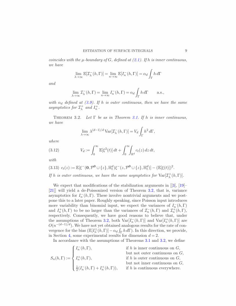
ESTIMATION OF SURFACE INTEGRALS 9
coincides with the µ-boundary of G, defined at (2.1). If h is inner continuous,we have
limλ→∞
E[I−λ (h,Γ)] = lim
n→∞E[I−n (h,Γ)] = αd
∫
ΓhdΓ
and
limλ→∞
I−λ (h,Γ) = lim
n→∞I−n (h,Γ) = αd
∫
ΓhdΓ a.s.,
with αd defined at (3.9). If h is outer continuous, then we have the sameasymptotics for I+
λ and I+n .
Theorem 3.2. Let Γ be as in Theorem 3.1. If h is inner continuous,we have
limλ→∞
λ(d−1)/dVar[I−λ (h,Γ)] = Vd
∫
Γh2 dΓ,
where
Vd :=
∫ ∞
0E[ξ2(t)]dt+
∫ ∞
0
∫
Rd
ct(z)dz dt,(3.12)
with
ct(z) := E[ξ−(0,P0 ∪ {z},Hdt )ξ
−(z,P0 ∪ {z},Hdt )]− (E[ξ(t)])2.(3.13)
If h is outer continuous, we have the same asymptotics for Var[I+λ (h,Γ)].
We expect that modifications of the stabilization arguments in [[3], [19]–[21]] will yield a de-Poissonized version of Theorem 3.2, that is, varianceasymptotics for I−n (h,Γ). These involve nontrivial arguments and we post-pone this to a later paper. Roughly speaking, since Poisson input introducesmore variability than binomial input, we expect the variances of I−n (h,Γ)and I+n (h,Γ) to be no larger than the variances of I−
n (h,Γ) and I+n (h,Γ),
respectively. Consequently, we have good reasons to believe that, underthe assumptions of Theorem 3.2, both Var[I−n (h,Γ)] and Var[I+n (h,Γ)] areO(n−(d−1)/d). We have not yet obtained analogous results for the rate of con-vergence for the bias (E[I±n (h,Γ)]−αd
∫
Γ hdΓ). In this direction, we provide,in Section 4, some experimental results for dimension d= 2.
In accordance with the assumptions of Theorems 3.1 and 3.2, we define
Sn(h,Γ) :=
I−n (h,Γ), if h is inner continuous on G,but not outer continuous on G,
I+n (h,Γ), if h is outer continuous on G,but not inner continuous on G,
12(I
−n (h,Γ) + I+n (h,Γ)), if h is continuous everywhere.
10 R. JIMENEZ AND J. E. YUKICH
In the light of our results and remarks, we propose to estimate the surfaceintegral
∫
Γ hdΓ by the strongly consistent sewing-based estimator
α−1d Sn(h,Γ).(3.14)
Since Theorems 3.1 and 3.2 only assume the rectifiability of Γ, the esti-mator (3.14) is applicable when the body G has sharp interior or exteriorcusps. In particular, it can be used for estimating the boundary measure ofsuch sets, an estimation problem in which previous methods [2, 8, 18] havedrawbacks. Under suitable conditions on the smoothing parameter, [10] alsodiscusses the consistency of the estimators based on the Minkowski contentfor a general class of bodies.
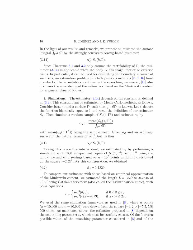
4. Simulations. The estimator (3.14) depends on the constant αd definedat (3.9). This constant can be estimated by Monte Carlo methods, as follows.Consider large n and a surface Γ0 such that
∫
Γ0 dΓ0 is known. Let 1 denote
the function identically equal to 1 and recall the definition of our estimatorSn. Then simulate a random sample of Sn(1,Γ0) and estimate αd by
αd :=mean(Sn(1,Γ0))
∫
Γ0 dΓ0
with mean(Sn(h,Γ0)) being the sample mean. Given αd and an arbitrary
surface Γ, the natural estimator of∫
Γ hdΓ is thus
α−1d Sn(h,Γ).(4.1)
Taking this procedure into account, we estimated α2 by performing asimulation with 1000 independent copies of Sn(1,Γ0), with Γ0 being theunit circle and with sewings based on n= 107 points uniformly distributedon the square [−2,2]2. For this configuration, we obtained
α2 = 1.1820.(4.2)
To compare our estimator with those based on empirical approximationof the Minkowski content, we estimated the length L= 12
√3≈ 20.7846 of
T , T being Catalan’s trisectrix (also called the Tschirnhausen cubic), withpolar equations
r =
{
sec3(θ/3), if 0< θ ≤ π,sec3((2π− θ)/3), if π < θ ≤ 2π.
We used the same simulation framework as used in [8], where n points(n= 10,000 and n= 30,000) were drawn from the square [−9,2]× [−5.5,5.5]500 times. As mentioned above, the estimator proposed in [8] depends onthe smoothing parameter ε, which must be carefully chosen. Of the fourteenpossible values of the smoothing parameter considered in [8] and of the
ESTIMATION OF SURFACE INTEGRALS 11
Table 1Mean and standard deviation of estimators based on the Minkowski content,with optimal smoothing parameter, and the sewing-based estimators over 500replications and simple sizes n= 10,000 and n= 30,000 (the true value is
12√3≈ 20.7846)
n mean(LMn (T )) std(LM
n (T )) mean(LSn(T )) std(LS
n(T ))
10,000 19.3679 1.0394 20.7030 0.314030,000 19.8237 1.0666 20.7328 0.2375
fourteen different corresponding estimators, we let LMn (T ) be the Minkowski
content estimator having, on average, the smallest bias, that is, the oneminimizing the difference between the expectation of the estimator and itstarget value. In Table 1, we compare LM
n (T ) with the sewing-based estimatorLSn(T ), namely
LSn(T ) = α−1
d Sn(1,T ).(4.3)
Roughly speaking, we improve the mean relative error (difference betweenexact and approximate mean value/exact value) by a factor of 10−3 and wesignificantly reduce the standard deviation.
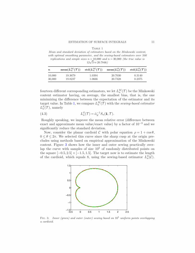
Now, consider the planar cardioid C with polar equation ρ = 1 + cos θ,0 ≤ θ ≤ 2π. We selected this curve since the sharp cusp at the origin pre-cludes using methods based on empirical approximation of the Minkowskicontent. Figure 3 shows how the inner and outer sewing practically over-lap the curve with samples of size 105 of randomly distributed points onthe square [−0.5,2.5]× [−1.5,1.5]. The target now is to estimate the lengthof the cardioid, which equals 8, using the sewing-based estimator LS
n(C).
Fig. 3. Inner (green) and outer (outer) sewing based on 105 uniform points overlappinga cardioid.
12 R. JIMENEZ AND J. E. YUKICH
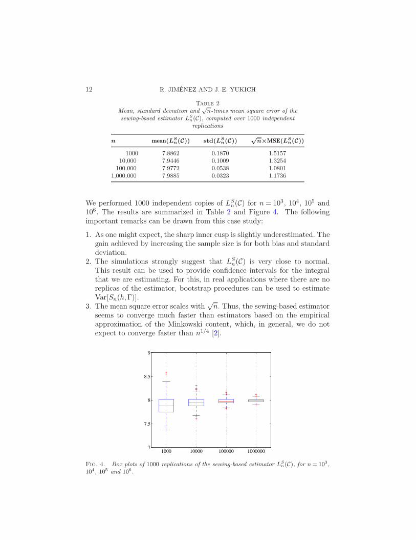
Table 2Mean, standard deviation and
√n-times mean square error of the
sewing-based estimator LSn(C), computed over 1000 independentreplications
n mean(LSn(C)) std(LS
n(C))√n×MSE(LS
n(C))
1000 7.8862 0.1870 1.515710,000 7.9446 0.1009 1.3254
100,000 7.9772 0.0538 1.08011,000,000 7.9885 0.0323 1.1736
We performed 1000 independent copies of LSn(C) for n= 103, 104, 105 and
106. The results are summarized in Table 2 and Figure 4. The followingimportant remarks can be drawn from this case study:
1. As one might expect, the sharp inner cusp is slightly underestimated. Thegain achieved by increasing the sample size is for both bias and standarddeviation.
2. The simulations strongly suggest that LSn(C) is very close to normal.
This result can be used to provide confidence intervals for the integralthat we are estimating. For this, in real applications where there are noreplicas of the estimator, bootstrap procedures can be used to estimateVar[Sn(h,Γ)].
3. The mean square error scales with√n. Thus, the sewing-based estimator
seems to converge much faster than estimators based on the empiricalapproximation of the Minkowski content, which, in general, we do notexpect to converge faster than n1/4 [2].
Fig. 4. Box plots of 1000 replications of the sewing-based estimator LSn(C), for n= 103,
104, 105 and 106.
ESTIMATION OF SURFACE INTEGRALS 13
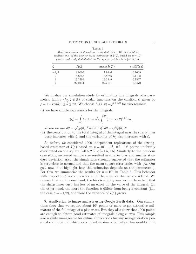
Table 3Mean and standard deviation, computed over 1000 independent
replications, of the sewing-based estimator of I(ζ), based on n= 104
points uniformly distributed on the square [−0.5,2.5]× [−1.5,1.5]
ζ I(ζ) mean(I(ζ)) std(I(ζ))
−1/2 8.0000 7.9446 0.10090 8.8858 8.8786 0.11381 13.3286 13.3349 0.18272 22.2144 22.2191 0.3470
We finalize our simulation study by estimating line integrals of a para-metric family {hζ , ζ ∈ R} of scalar functions on the cardioid C given by
ρ= 1+ cos θ,0≤ θ ≤ 2π. We choose hζ(x, y) = ρζ+1/2 for two reasons:
(i) we have simple expressions for the integrals
I(ζ) =
∫
Chζ dC =
√2
∫ 2π
0(1 + cos θ)1+ζ dθ,
where we use dC =√
(ρ(θ))2 + (ρ′(θ))2 dθ =√
2ρ(θ)dθ;(ii) the contribution to the total integral of the integral near the sharp inner
cusp increases with ζ , and the variability of hζ also increases with ζ .
As before, we considered 1000 independent replications of the sewing-based estimator of I(ζ) based on n = 103, 104, 105, 106 points uniformlydistributed on the square [−0.5,2.5] × [−1.5,1.5]. Similarly to the previouscase study, increased sample size resulted in smaller bias and smaller stan-dard deviation. Also, the simulations strongly suggested that the estimatoris very close to normal and that the mean square error scales with
√n. Our
goal now is to highlight how the estimation depends on the parameter ζ .For this, we summarize the results for n = 104 in Table 3. This behaviorwith respect to ζ is common for all of the n values that we considered. Weremark that, on the one hand, the bias is slightly smaller, to the extent thatthe sharp inner cusp has less of an effect on the value of the integral. Onthe other hand, the more the function h differs from being a constant (i.e.,
the case ζ =−1/2), the more the variance of I(ζ) grows.
5. Application to image analysis using Google Earth data. Our simula-tions show that we require about 105 points or more to get attractive esti-mators of the full image of a planar set. But they also show that 1000 pointsare enough to obtain good estimates of integrals along curves. This samplesize is quite manageable for online applications for any new-generation per-sonal computer, on which a compiled version of our algorithm would run in
14 R. JIMENEZ AND J. E. YUKICH
less than a second. Even n= 104 could be implemented for snapshot queries.Next, we discuss an application to image analysis using Google Earth data.Quite possibly, Google provides a sharp image of the area around your res-idence or workplace, but what can you infer from the image of the mostinaccessible regions of the planet, including, for example, the coast of theAral Sea?
According to the United Nations, the disappearance of the Aral Sea, oncethe fourth largest inland body of water on the planet, is the worst man-madeenvironmental disaster of the 20th century. It is estimated that the size of theAral Sea has fallen by more than 60% since the 1960s. Water withdrawal forirrigation has caused a dramatic fall in the water level, revealing a fascinatinggeology of cliffs overlooking the Aral Sea. What is the mean height of thecliffs along a long waterfront? How irregular are they? Google Earth provideselevation information for any pixel and, from its color, we can determinewhether it is in the Aral Sea or not. This scenario fits our sampling modeland thus we may use sewings to estimate the mean and variance of theelevations of cliffs along waterfronts. Both parameters are related to commontopographic measures. According to [13], the standard deviation of elevationprovides one of the most stable measures of the vertical variability of atopographic surface. On the other hand, the elevation mean is related to theelevation-relief ratio, namely
elevation mean – elevation min.
elevation max. – elevation min.,
which has been computed in the past using a point-sampling technique,rather than planimetry [22].
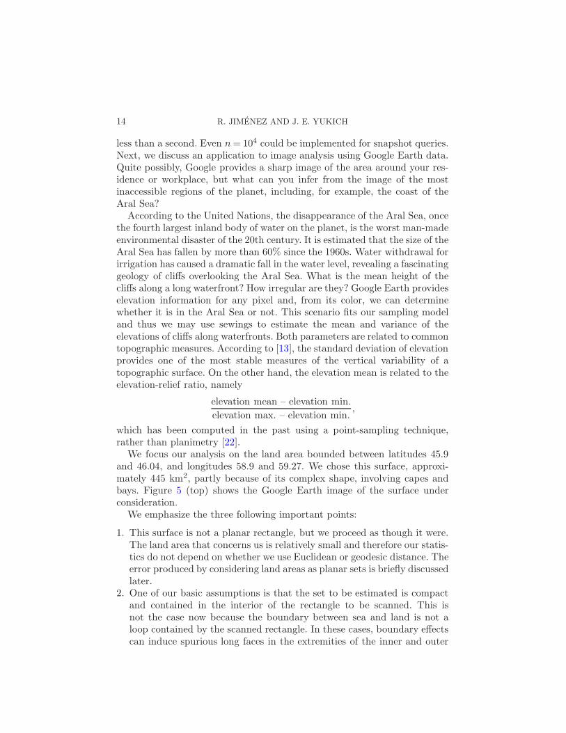
We focus our analysis on the land area bounded between latitudes 45.9and 46.04, and longitudes 58.9 and 59.27. We chose this surface, approxi-mately 445 km2, partly because of its complex shape, involving capes andbays. Figure 5 (top) shows the Google Earth image of the surface underconsideration.
We emphasize the three following important points:
1. This surface is not a planar rectangle, but we proceed as though it were.The land area that concerns us is relatively small and therefore our statis-tics do not depend on whether we use Euclidean or geodesic distance. Theerror produced by considering land areas as planar sets is briefly discussedlater.
2. One of our basic assumptions is that the set to be estimated is compactand contained in the interior of the rectangle to be scanned. This isnot the case now because the boundary between sea and land is not aloop contained by the scanned rectangle. In these cases, boundary effectscan induce spurious long faces in the extremities of the inner and outer
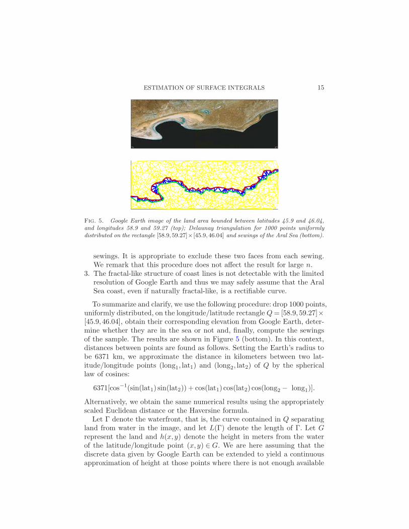
ESTIMATION OF SURFACE INTEGRALS 15
Fig. 5. Google Earth image of the land area bounded between latitudes 45.9 and 46.04,and longitudes 58.9 and 59.27 (top); Delaunay triangulation for 1000 points uniformlydistributed on the rectangle [58.9,59.27]× [45.9,46.04] and sewings of the Aral Sea (bottom).
sewings. It is appropriate to exclude these two faces from each sewing.We remark that this procedure does not affect the result for large n.
3. The fractal-like structure of coast lines is not detectable with the limitedresolution of Google Earth and thus we may safely assume that the AralSea coast, even if naturally fractal-like, is a rectifiable curve.
To summarize and clarify, we use the following procedure: drop 1000 points,uniformly distributed, on the longitude/latitude rectangle Q= [58.9,59.27]×[45.9,46.04], obtain their corresponding elevation from Google Earth, deter-mine whether they are in the sea or not and, finally, compute the sewingsof the sample. The results are shown in Figure 5 (bottom). In this context,distances between points are found as follows. Setting the Earth’s radius tobe 6371 km, we approximate the distance in kilometers between two lat-itude/longitude points (long1, lat1) and (long2, lat2) of Q by the sphericallaw of cosines:
6371[cos−1(sin(lat1) sin(lat2)) + cos(lat1) cos(lat2) cos(long2 − long1)].
Alternatively, we obtain the same numerical results using the appropriatelyscaled Euclidean distance or the Haversine formula.
Let Γ denote the waterfront, that is, the curve contained in Q separatingland from water in the image, and let L(Γ) denote the length of Γ. Let Grepresent the land and h(x, y) denote the height in meters from the waterof the latitude/longitude point (x, y) ∈ G. We are here assuming that thediscrete data given by Google Earth can be extended to yield a continuousapproximation of height at those points where there is not enough available
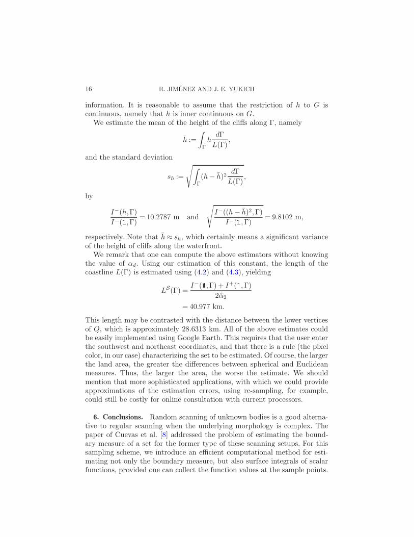
16 R. JIMENEZ AND J. E. YUKICH
information. It is reasonable to assume that the restriction of h to G iscontinuous, namely that h is inner continuous on G.
We estimate the mean of the height of the cliffs along Γ, namely
h :=
∫
Γh
dΓ
L(Γ),
and the standard deviation
sh :=
√
∫
Γ(h− h)2
dΓ
L(Γ),
by
I−(h,Γ)
I−(1,Γ) = 10.2787 m and
√
I−((h− h)2,Γ)
I−(1,Γ) = 9.8102 m,
respectively. Note that h≈ sh, which certainly means a significant varianceof the height of cliffs along the waterfront.
We remark that one can compute the above estimators without knowingthe value of αd. Using our estimation of this constant, the length of thecoastline L(Γ) is estimated using (4.2) and (4.3), yielding
LS(Γ) =I−(1,Γ)+ I+(1,Γ)
2α2
= 40.977 km.
This length may be contrasted with the distance between the lower verticesof Q, which is approximately 28.6313 km. All of the above estimates couldbe easily implemented using Google Earth. This requires that the user enterthe southwest and northeast coordinates, and that there is a rule (the pixelcolor, in our case) characterizing the set to be estimated. Of course, the largerthe land area, the greater the differences between spherical and Euclideanmeasures. Thus, the larger the area, the worse the estimate. We shouldmention that more sophisticated applications, with which we could provideapproximations of the estimation errors, using re-sampling, for example,could still be costly for online consultation with current processors.
6. Conclusions. Random scanning of unknown bodies is a good alterna-tive to regular scanning when the underlying morphology is complex. Thepaper of Cuevas et al. [8] addressed the problem of estimating the bound-ary measure of a set for the former type of these scanning setups. For thissampling scheme, we introduce an efficient computational method for esti-mating not only the boundary measure, but also surface integrals of scalarfunctions, provided one can collect the function values at the sample points.
ESTIMATION OF SURFACE INTEGRALS 17
We discuss conditions for getting strong consistency, as well as some issuesrelated to the rate of convergence of our estimators. Our proofs rely onpoint process methods, including weak convergence of point processes andstabilization methods.
We perform a simulation study to compare our estimators with previousestimators of boundary lengths of sets, concluding that the sewing-based es-timators (4.1) significantly reduce the errors and computation times, whileincreasing precision. We complete our simulation study by estimating bound-ary lengths of sets with sharp cusps, as well as the integrals of scalar func-tions on the boundaries of these sets, always obtaining good results.
An online application to image analysis using Google Earth data is dis-cussed. In particular, a complex waterfront of the Aral Sea, approximately41 km according to our estimators, is analyzed. Specifically, we estimatesurface integrals related to the mean and standard deviation of the heightof the irregular cliffs facing the sea line.
7. Proofs and technical results. As indicated at the outset, our approachmakes use of stabilizing functionals ξ, where ξ(x,X ) is a translation invariantfunctional defined on pairs (x,X ), where x ∈R
d and X ⊂Rd is locally finite.
Translation invariance means that ξ(x,X ) = ξ(x+ y,x+X ) for all y ∈ Rd.
We recall a few facts about such functionals [[3], [19]–[21]]. As in [19], weconsider the following metric on the space L of locally finite subsets of Rd:
D(A,A′) := (max{K ∈N :A∩BK(0) =A′ ∩BK(0)})−1.(7.1)
We say that ξ(·, ·) stabilizes on a homogeneous Poisson point process Pif, for all x ∈R
d, there is an a.s. finite R :=R(x,P) such that
ξ(x,P ∩BR(x)) = ξ(x, [P ∩BR(x)] ∪A)
for all A⊂ (BR(x))c. Recall that P0 := P ∪ {0}. Now, whenever ξ(·, ·) sat-
isfies stabilization, then P0 is a continuity point for the function g(A) :=ξ(0,A) with respect to the topology on L induced by D. Thus, by the contin-uous mapping theorem (Proposition A2.3V on page 394 of [11]), if Yn, n≥ 1,
is a sequence of random point measures satisfying YnD−→P0 as n→∞, then
ξ(0,Yn)D−→ ξ(0,P0); see [19] for details.
Thus, if Uk, k ≥ 1, are i.i.d. uniform on the unit cube with Un := {Uk}nk=1
and if ξ is translation invariant so that ξ(n1/dU1, n1/dUn) = ξ(0, n1/d(Un −
U1)), then, since the shifted and dilated random point measures n1/d(Un −U1) satisfy the convergence n1/d(Un −U1)
D−→P0, it follows from stabiliza-tion that, as n→∞,
ξ(n1/dUk, n1/dUn)
D−→ ξ(0,P0).(7.2)
18 R. JIMENEZ AND J. E. YUKICH
This result is central to proving the weak law of large numbers [21],
n−1n∑
k=1
ξ(n1/dUk, n1/dUn)
P→ E[ξ(0,P0)].(7.3)
The analogous convergence result for the two-dimensional vector
[ξ(n1/dUk, n1/dUn), ξ(n
1/dUj , n1/dUn)], k 6= j,
is likewise central to showing variance asymptotics and central limit theo-rems [3, 19] for the sums in (7.3).
One of the main features of our proofs is that if ξ is stabilizing, if Yn, n≥ 1,is a sequence of point processes on sets increasing up to the half-space H
which is a translation/rotation of Hd0 :=R
d−1× (−∞,0] and if YnD−→P ∩H
as n→∞, then, subject to the proper scaling, there exist limit results for ξanalogous to those at (7.3). Our goal is to make these ideas precise.
We prove our main results for the functional ξ−. Identical results hold forthe functional ξ+ and the proofs for it are analogous. We henceforth simplywrite ξ for ξ− and I for I−.
To demonstrate the required asymptotics for (3.1) and (3.2), and to takeadvantage of the ideas just discussed, it is natural to parametrize points inQ as follows. First, assume without loss of generality that Q has Lebesguemeasure equal to 1. Let M(G) be the medial axis of G, that is, the closure ofthe set of all points in G with more than one closest point on Γ. In general,M(G) is a nonregular (d − 1)-dimensional surface with null d-dimensionalLebesgue measure. We refer the reader to [7] for all matters concerning thetheory of medial axes.
Let Γ0 ⊂ Γ be the subset of Γ where there is no uniquely defined tangentplane. Then, Hd−1(Γ0) = 0 by assumption. Consider the subset G1 of G \M(G) consisting of points x such that there is a γ ∈ Γ \ Γ0 with x − γorthogonal to the tangent plane at γ and γ := γ(x) is the boundary pointclosest to x. Let G0 be the complement of G1 with respect to G \M(G).
For all t > 0, consider the level sets Γ(t) := {x ∈ G\M(G) :d(x,Γ) = t},where d(x,Γ) denotes the distance between x and Γ. Except possibly on aLebesgue null subset of G1, we may uniquely parameterize points x ∈ G1
as x(γ, t), where γ is the boundary point closest to x and t := ‖x− γ‖. SetΓ(0) = Γ. Let Γ1(t) := Γ(t)∩G1 and Γ0(t) := Γ(t)∩G0. For each γ ∈ Γ \Γ0,let Rγ be the distance between γ and M(G), measured along the orthogonalto the tangent plane to Γ at γ. Define D := supγ∈ΓRγ .
For any integrable function g :Q→ R, an application of the co-area for-mula (see Theorem 3.2.12 and Lemma 3.2.34 in [14]) for the distance functionf(x) := d(x,Γ) gives
∫
Gg(x)dx=
∫ D
0
∫
Γ(t)g(x)Hd−1(dx)dt
ESTIMATION OF SURFACE INTEGRALS 19
since |∇(f(x))| ≡ 1 a.e. This yields the scaled volume identity
n1/d
∫
Gg(x)dx=
∫ Dn1/d
0
[∫
Γ1(tn−1/d)g(x(γ, tn−1/d))Hd−1(dx)
]
dt
(7.4)
+
∫ Dn1/d
0
[∫
Γ0(tn−1/d)g(x)Hd−1(dx)
]
dt.
We may similarly write
n1/d
∫
Gc
g(x)dx=
∫ D′n1/d
0
[∫
Γ′1(tn
−1/d)g(x(γ, tn−1/d))Hd−1(dx)
]
dt
(7.5)
+
∫ D′n1/d
0
[∫
Γ′0(tn
−1/d)g(x)Hd−1(dx)
]
dt,
where D′,Γ′1(·) and Γ′
0(·) are now the analogs of D′,Γ1(·) and Γ0(·), respec-tively.
To simplify the notation and to set the stage for developing the analog of(7.2), we define, for all x ∈G1, the shifted and n1/d-dilated binomial pointmeasures
Pn(γ, t) := n1/d(Xn−1 − x(γ, tn−1/d)) ∪ {0},(7.6)
together with the shifted and dilated bodies
Gn(γ, t) := n1/d(G− x(γ, tn−1/d)).(7.7)
We similarly define the shifted and λ1/d-dilated Poisson point measures
Pλ(γ, t) := λ1/d(Pλ − x(γ, tλ−1/d)) ∪ {0}(7.8)
and the shifted and dilated bodies
Gλ(γ, t) := λ1/d(G− x(γ, tλ−1/d)).(7.9)
More generally, for all x ∈G, we write
Pn(x) := n1/d(Xn−1 − x)∪ {0}and similarly for Gn(x),Pλ(x) and Gλ(x).
Roughly speaking, the dilated bodiesGn(γ, t) are converging locally aroundx(γ, tn−1/d) to a half-space, whereas the restrictions of the point processesPn(γ, t) to Gn(γ, t) are converging to a homogeneous point process on thishalf-space [see (7.12)].
The next result, a consequence of this observation, is similar to (7.2) and isthe key to all that follows. It shows that for all γ ∈ Γ \Γ0 and t ∈ (0,∞), theHausdorff measure of faces incident to 0 and belonging to the inner sewingS−(Pn(γ, t), ∂Gn(γ, t)) converges in distribution to the Hausdorff measureof faces incident to 0 and belonging to the inner sewing S−(P0, ∂Hd
−t).
20 R. JIMENEZ AND J. E. YUKICH
Lemma 7.1. For all γ ∈ Γ \ Γ0 and t ∈ (0,∞), we have
ξ(0,Pn(γ, t),Gn(γ, t))D−→ ξ(t); ξ(0,Pλ(γ, t),Gλ(γ, t))
D−→ ξ(t).(7.10)
Proof. We will only prove the first result since the second follows byidentical methods. Using a rotation if necessary, we will, without loss ofgenerality, assume that the vector 0− (γ,0) is orthogonal to the boundaryof the half-space H
d−t.
For an arbitrary point set Y ⊂Rd and bodyD, let ξB(y,Y∩D) be the sum
of the Hausdorff measures of the faces of the Delaunay triangulation of Y∩Dlying wholly inside D and incident to y ∈ Y . Recall that, by construction,the faces giving nonzero contribution to ξ(0,Pn(γ, t),Gn(γ, t)) have verticesbelonging to Gn(γ, t). Since the boundary of Gn(γ, t) is differentiable, itfollows for large enough n that these faces will eventually belong entirely toGn(γ, t). In other words,
limn→∞
|ξ(0,Pn(γ, t),Gn(γ, t))− ξB(0,Pn(γ, t) ∩Gn(γ, t))|= 0 a.s.
(7.11)Since 0 is at a distance t from the boundary of Gn(γ, t), it follows that
the value of ξB at 0 with respect to H ∩ (Rd−1 ∩ (−∞, t]) is determinedby the points of H∩ (Rd−1 ∩ (−∞, t]) in a ball centered at 0 and of radiusR := max(t,R0), where R0 is the stabilization radius at 0 for the graph ofthe standard Delaunay triangulation of H∪0. Thus, reasoning exactly as in(7.1) and (7.2), we have that H∩ (Rd−1 ∩ (−∞, t]) is a continuity point forthe function g(A) := ξB(0,A) with respect to the topology on L induced bythe metric D at (7.1). Since
Pn(γ, t)∩Gn(γ, t)D−→H∩ (Rd−1 ∩ (−∞, t]),(7.12)
it therefore follows by the continuous mapping theorem that
ξB(0,Pn(γ, t)∩Gn(γ, t))D−→ ξB(0,H∩ (Rd−1 ∩ (−∞, t])) = ξ(t).
Combining this with (7.11), we have ξ(0,Pn(γ, t),Gn(γ, t))D−→ ξ(t), which
completes the proof. �
Given (7.10), one has convergence of the corresponding expectations in(7.10), provided the random variables satisfy the customary uniform inte-grability condition. This is the content of the next lemma.
Lemma 7.2. For all γ ∈ Γ \ Γ0 and all t > 0, we have
limn→∞
E[ξ(0,Pn(γ, t),Gn(γ, t))] = limλ→∞
E[ξ(0,Pλ(γ, t),Gλ(γ, t))] = E[ξ(t)].
ESTIMATION OF SURFACE INTEGRALS 21
Proof. It is straightforward that the empty sphere criterion charac-terizing Delaunay triangulations (see, e.g., Chapter 4 of [24]) implies that,uniformly in t, the volume of a Delaunay simplex in Pn(γ, t) has expo-nentially decaying tails, this being equivalent to the tail probability that acircumcircle (circumsphere in dimension greater than 2) contains no pointsfrom the binomial point process Pn(γ, t). It follows that for p > 0, there is aconstant C(p) such that
supn
sup(γ,t)
E[|ξ(0,Pn(γ, t),Gn(γ, t))|p]≤C(p),(7.13)
showing that
{ξ(0,Pn(γ, t),Gn(γ, t)), n≥ 1}are uniformly integrable. By Lemma 7.1, we obtain the desired convergenceof E[ξ(0,Pn(γ, t),Gn(γ, t))]. The convergence of E[ξ(0,Pλ(γ, t),Gλ(γ, t))] fol-lows using identical methods. �
The next two lemmas are also consequences of exponential decay of thevolume of the circumspheres not containing points from n1/dXn. The nextresult shows that the expectations appearing in Lemma 7.2 are uniformlybounded, a technical result foreshadowing the upcoming use of the domi-nated convergence theorem.
Lemma 7.3. There is an integrable function F : [0,∞) → [0,∞), withexponentially decaying tails, such that
supn
supx∈Γ(tn−1/d)
E[ξ(0,Pn(x),Gn(x))]≤ F (t)
and
supλ
supx∈Γ(tλ−1/d)
E[ξ(0,Pλ(x),Gλ(x))]≤ F (t).
Proof. For all x∈ Γ(tn−1/d), let
E(x) := {0 belongs to a facef of a simplex in D(Pn(x)), f ∩ ∂Hdt 6=∅}.
By definition, ξ vanishes on Ec(x). It is easy to see that P [E(x)] has expo-nentially decaying tails in t, uniformly in n and γ. The first result follows byconsidering ξ(0,Pn(x),Gn(x))1(E(x)), and applying the Cauchy–Schwarzinequality and the bound (7.13) with p= 2. The second result follows simi-larly. �
Our last lemma provides a high probability bound on the diameter ofDelaunay simplices, a result which follows immediately from the exponential
22 R. JIMENEZ AND J. E. YUKICH
decay of the volume of spheres not containing points from Xn or Pλ. In otherwords, making use of the bounds P [Pλ ∩Br(x) =∅] = exp(−λrdvd), wherevd is the volume of the unit radius d-dimensional ball, as well as the boundsP [Xn ∩Br(x) =∅] = (1− rdvd)
n, we obtain the following result.
Lemma 7.4. For any constant A > 0, there is a constant C > 0 suchthat, with probability exceeding 1− n−A, the diameter of all Delaunay sim-plices in D(Xn) is bounded by C(logn/n)1/d. Thus, with probability exceeding1− n−A, we have
supi≤n
ξ(Xi,Xn,G)≤C(logn/n)(d−1)/d
and
supx∈Pλ
ξ(x,Pλ,G)≤C(logλ/λ)(d−1)/d.
We now have all of the ingredients needed to prove Theorem 3.1.
Proof of Theorem 3.1. The proof has two parts: the first showsexpectation convergence and the second uses concentration inequalities todeduce the a.s. convergence.
Part I. We use the above lemmas (binomial input) to first show thatlimn→∞E[In(h,Γ)] = αd
∫
Γ hdΓ for h inner continuous, recalling that we no-
tationally simplify ξ− to ξ and I−n to In. We omit the proof of limλ→∞E[I−λ (h,
Γ)] = αd
∫
Γ hdΓ as it follows verbatim, using instead the Poisson input ver-sions of the above lemmas.
Note that ξ(X1,Xn,G) = 0 if X1 /∈G. Using (3.4) and conditioning on X1,we have
E[In(h,Γ)] = nE[h(X1)ξ(X1,Xn,G)]
= n1/dE[h(X1)ξ(0, n
1/d(Xn −X1), n1/d(G−X1))]
= n1/d
∫
Gh(x)E[ξ(0, n1/d(Xn−1 − x)∪ {0}, n1/d(G− x))]dx.
Using the scaled volume identity (7.4) and putting, for all x ∈G,
Gn(x) := h(x)E[ξ(0, n1/d(Xn−1 − x)∪ {0}, n1/d(G− x))],
we get that
E[In(h,Γ)] =
∫ Dn1/d
0
∫
Γ1(tn−1/d)Gn(x)Hd−1(dx)dt
(7.14)
+
∫ Dn1/d
0
∫
Γ0(tn−1/d)Gn(x)Hd−1(dx)dt.
ESTIMATION OF SURFACE INTEGRALS 23
The proof of expectation convergence will be complete once we show thatthe two integrals in (7.14) converge to αd
∫
Γ h(γ)Hd−1(dγ) and zero, respec-tively.
We first consider the first integral in (7.14). For fixed t > 0 and all n, thereis an a.e. C1 mapping fn : Γ→ Γ1(tn
−1/d) of Γ onto the level set Γ1(tn−1/d).
To prepare for an application of the dominated convergence theorem, wenext show, for each t > 0, that as n→∞,
∫
Γ1(tn−1/d)Gn(x)Hd−1(dx)→
∫
Γh(γ)E[(ξ(t))]Hd−1(dγ).(7.15)
To see this, write the difference of the integrals in (7.15) as the sum of∫
Γ1(tn−1/d)Gn(x)Hd−1(dx)−
∫
ΓGn(fn(γ))Hd−1(dγ)(7.16)
and∫
ΓGn(fn(γ))Hd−1(dγ)−
∫
Γh(γ)E[(ξ(t))]Hd−1(dγ).(7.17)
By a change of variables, the difference (7.16) equals∫
ΓGn(fn(γ))[Hd−1(dfn(γ))−Hd−1(dγ)].
By the a.e. smoothness of Γ, we have Hd−1(dfn(γ)) = (1 + ǫn(γ))Hd−1(dγ)a.e., where ǫn(γ) goes to zero as n→∞. By (7.13), we have
supn
supγ∈Γ
|Gn(fn(γ))| ≤C(1)‖h‖∞
and so the difference (7.16) goes to zero. Next, consider the difference (7.17).Recalling that t is fixed, for all γ ∈ Γ we write fn(γ) = x(γ, tn−1/d). Asn → ∞, we have h(x(γ, tn−1/d)) → h(x(γ,0)) = h(γ), by inner continuityof h. Combining this with Lemma 7.2, we get, for all x ∈ Γ1(tn
−1/d) withx= x(γ, tn−1/d), that Gn(x) converges to h(γ)E[ξ(t)] and so, by the boundedconvergence theorem, the difference (7.17) goes to zero as n → ∞. Thus,(7.15) holds.
By Lemma 7.3, we have, for fixed t > 0,∫
Γ1(tn−1/d)Gn(x)Hd−1(dx)≤ ‖h‖∞ × sup
n(Hd−1(Γ(tn−1/d)))× F (t).(7.18)
By the boundedness of h and Hd−1(Γ), the right-hand side of (7.18) is inte-grable in t and thus the dominated convergence theorem implies that
∫ Dn1/d
0
∫
Γ(tn−1/d)[h(x(γ, tn−1/d))E[ξ(0,Pn(γ, t),Gn(γ, t))]]Hd−1(dx)dt
24 R. JIMENEZ AND J. E. YUKICH
converges to∫ ∞
0
∫
Γh(γ)E[ξ(t)]Hd−1(dx)dt=
∫ ∞
0E[ξ(t)]dt
∫
Γh(γ)Hd−1(dγ),
as desired.Finally, we show that the second integral in (7.14) goes to zero as n→∞.
For fixed t > 0, the inside integrals in (7.14) are also bounded by the right-hand side of (7.18). Since Hd−1(Γ0(tn
−1/d))→ 0 as n→∞, the dominatedconvergence theorem gives that the second integral in (7.14) converges tozero. This completes the proof of expectation convergence.
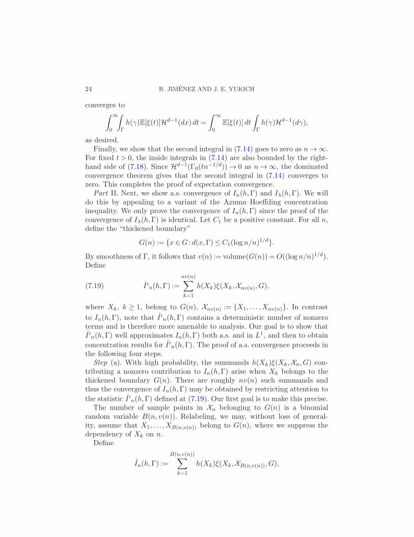
Part II. Next, we show a.s. convergence of In(h,Γ) and Iλ(h,Γ). We willdo this by appealing to a variant of the Azuma–Hoeffding concentrationinequality. We only prove the convergence of In(h,Γ) since the proof of theconvergence of Iλ(h,Γ) is identical. Let C1 be a positive constant. For all n,define the “thickened boundary”
G(n) := {x ∈G :d(x,Γ)≤C1(logn/n)1/d}.
By smoothness of Γ, it follows that v(n) := volume(G(n)) =O((logn/n)1/d).Define
I ′n(h,Γ) :=
nv(n)∑
k=1
h(Xk)ξ(Xk,Xnv(n),G),(7.19)
where Xk, k ≥ 1, belong to G(n), Xnv(n) := {X1, . . . ,Xnv(n)}. In contrast
to In(h,Γ), note that I ′n(h,Γ) contains a deterministic number of nonzeroterms and is therefore more amenable to analysis. Our goal is to show thatI ′n(h,Γ) well approximates In(h,Γ) both a.s. and in L1, and then to obtain
concentration results for I ′n(h,Γ). The proof of a.s. convergence proceeds inthe following four steps.
Step (a). With high probability, the summands h(Xk)ξ(Xk,Xn,G) con-tributing a nonzero contribution to In(h,Γ) arise when Xk belongs to thethickened boundary G(n). There are roughly nv(n) such summands andthus the convergence of In(h,Γ) may be obtained by restricting attention to
the statistic I ′n(h,Γ) defined at (7.19). Our first goal is to make this precise.The number of sample points in Xn belonging to G(n) is a binomial
random variable B(n, v(n)). Relabeling, we may, without loss of general-ity, assume that X1, . . . ,XB(n,v(n)) belong to G(n), where we suppress thedependency of Xk on n.
Define
In(h,Γ) :=
B(n,v(n))∑
k=1
h(Xk)ξ(Xk,XB(n,v(n)),G),
ESTIMATION OF SURFACE INTEGRALS 25
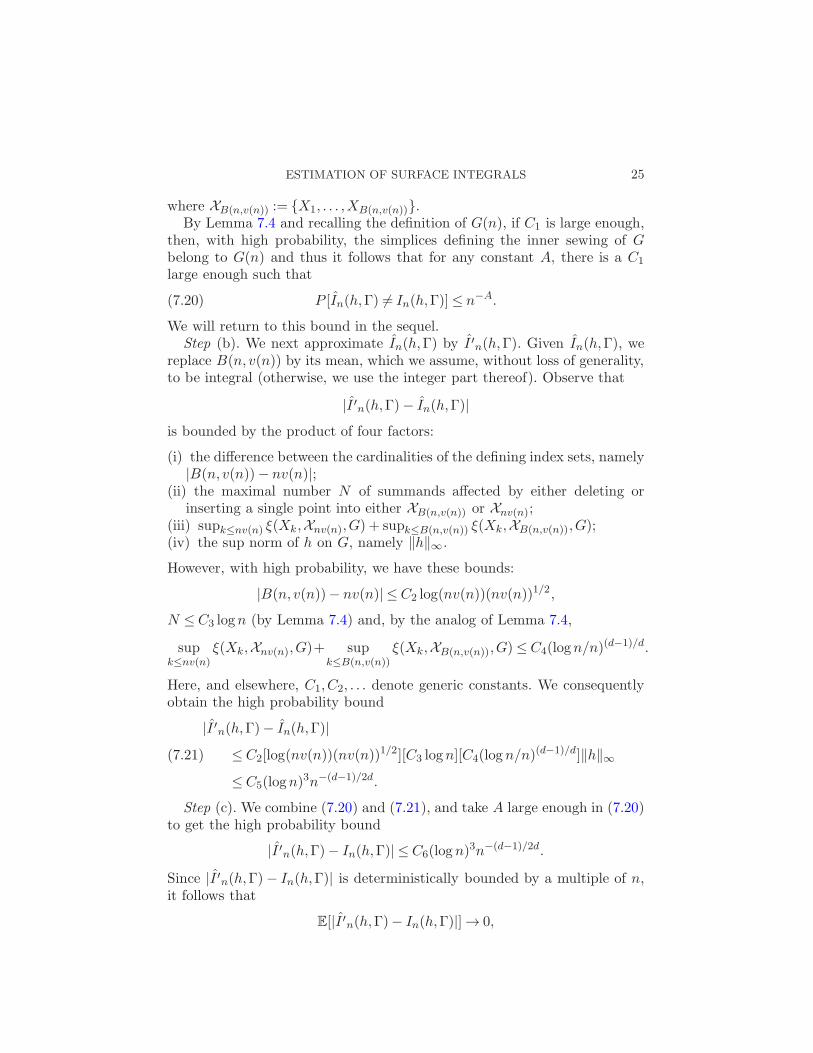
where XB(n,v(n)) := {X1, . . . ,XB(n,v(n))}.By Lemma 7.4 and recalling the definition of G(n), if C1 is large enough,
then, with high probability, the simplices defining the inner sewing of Gbelong to G(n) and thus it follows that for any constant A, there is a C1
large enough such that
P [In(h,Γ) 6= In(h,Γ)]≤ n−A.(7.20)
We will return to this bound in the sequel.Step (b). We next approximate In(h,Γ) by I ′n(h,Γ). Given In(h,Γ), we
replace B(n, v(n)) by its mean, which we assume, without loss of generality,to be integral (otherwise, we use the integer part thereof). Observe that
|I ′n(h,Γ)− In(h,Γ)|is bounded by the product of four factors:
(i) the difference between the cardinalities of the defining index sets, namely|B(n, v(n))− nv(n)|;
(ii) the maximal number N of summands affected by either deleting orinserting a single point into either XB(n,v(n)) or Xnv(n);
(iii) supk≤nv(n) ξ(Xk,Xnv(n),G) + supk≤B(n,v(n)) ξ(Xk,XB(n,v(n)),G);(iv) the sup norm of h on G, namely ‖h‖∞.
However, with high probability, we have these bounds:
|B(n, v(n))− nv(n)| ≤C2 log(nv(n))(nv(n))1/2,
N ≤C3 logn (by Lemma 7.4) and, by the analog of Lemma 7.4,
supk≤nv(n)
ξ(Xk,Xnv(n),G)+ supk≤B(n,v(n))
ξ(Xk,XB(n,v(n)),G)≤C4(logn/n)(d−1)/d.
Here, and elsewhere, C1,C2, . . . denote generic constants. We consequentlyobtain the high probability bound
|I ′n(h,Γ)− In(h,Γ)|≤C2[log(nv(n))(nv(n))
1/2][C3 logn][C4(logn/n)(d−1)/d]‖h‖∞(7.21)
≤C5(logn)3n−(d−1)/2d.
Step (c). We combine (7.20) and (7.21), and take A large enough in (7.20)to get the high probability bound
|I ′n(h,Γ)− In(h,Γ)| ≤C6(logn)3n−(d−1)/2d.
Since |I ′n(h,Γ)− In(h,Γ)| is deterministically bounded by a multiple of n,it follows that
E[|I ′n(h,Γ)− In(h,Γ)|]→ 0,
26 R. JIMENEZ AND J. E. YUKICH
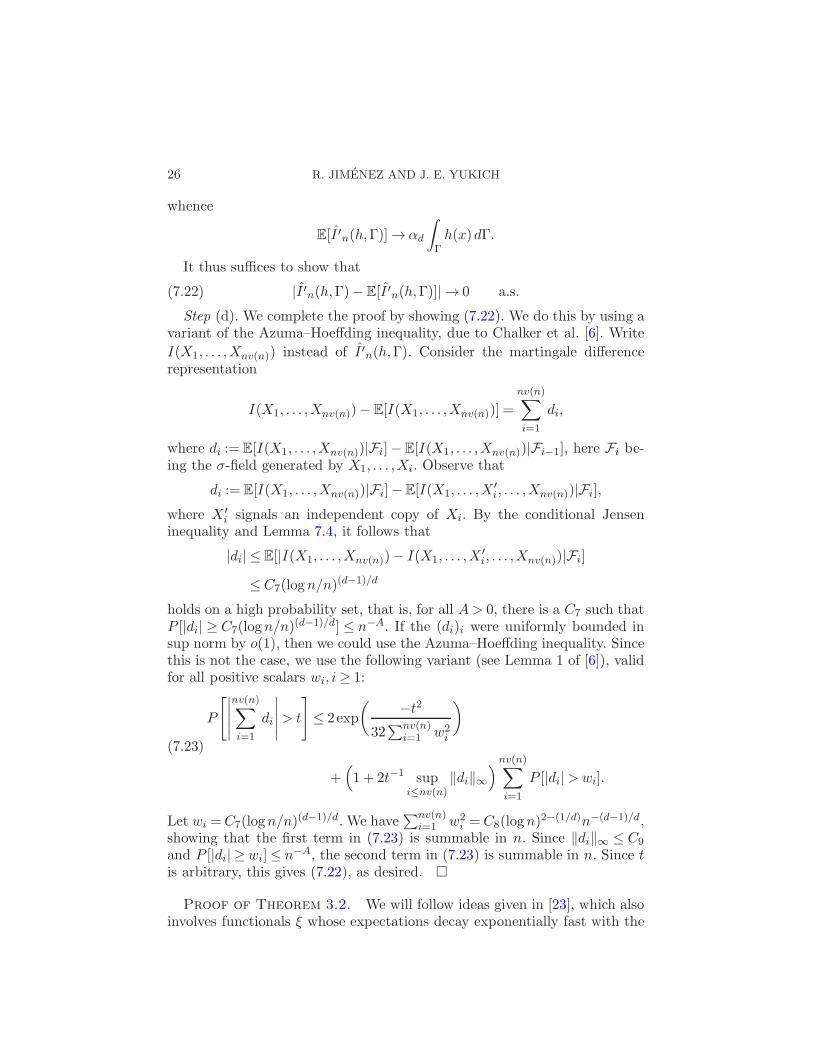
whence
E[I ′n(h,Γ)]→ αd
∫
Γh(x)dΓ.
It thus suffices to show that
|I ′n(h,Γ)−E[I ′n(h,Γ)]| → 0 a.s.(7.22)
Step (d). We complete the proof by showing (7.22). We do this by using avariant of the Azuma–Hoeffding inequality, due to Chalker et al. [6]. Write
I(X1, . . . ,Xnv(n)) instead of I ′n(h,Γ). Consider the martingale differencerepresentation
I(X1, . . . ,Xnv(n))− E[I(X1, . . . ,Xnv(n))] =
nv(n)∑
i=1
di,
where di := E[I(X1, . . . ,Xnv(n))|Fi]− E[I(X1, . . . ,Xnv(n))|Fi−1], here Fi be-ing the σ-field generated by X1, . . . ,Xi. Observe that
di := E[I(X1, . . . ,Xnv(n))|Fi]−E[I(X1, . . . ,X′i, . . . ,Xnv(n))|Fi],
where X ′i signals an independent copy of Xi. By the conditional Jensen
inequality and Lemma 7.4, it follows that
|di| ≤ E[|I(X1, . . . ,Xnv(n))− I(X1, . . . ,X′i, . . . ,Xnv(n))|Fi]
≤C7(logn/n)(d−1)/d
holds on a high probability set, that is, for all A> 0, there is a C7 such thatP [|di| ≥ C7(logn/n)
(d−1)/d] ≤ n−A. If the (di)i were uniformly bounded insup norm by o(1), then we could use the Azuma–Hoeffding inequality. Sincethis is not the case, we use the following variant (see Lemma 1 of [6]), validfor all positive scalars wi, i≥ 1:
P
[∣
∣
∣
∣
∣
nv(n)∑
i=1
di
∣
∣
∣
∣
∣
> t
]
≤ 2exp
( −t2
32∑nv(n)
i=1 w2i
)
(7.23)
+(
1 + 2t−1 supi≤nv(n)
‖di‖∞)
nv(n)∑
i=1
P [|di|>wi].
Let wi =C7(logn/n)(d−1)/d. We have
∑nv(n)i=1 w2
i =C8(logn)2−(1/d)n−(d−1)/d,
showing that the first term in (7.23) is summable in n. Since ‖di‖∞ ≤ C9
and P [|di| ≥wi]≤ n−A, the second term in (7.23) is summable in n. Since tis arbitrary, this gives (7.22), as desired. �
Proof of Theorem 3.2. We will follow ideas given in [23], which alsoinvolves functionals ξ whose expectations decay exponentially fast with the
ESTIMATION OF SURFACE INTEGRALS 27
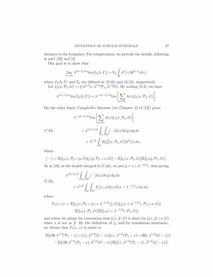
distance to the boundary. For completeness, we provide the details, followingin part [19] and [4].
Our goal is to show that
limλ→∞
λ(d−1)/dVar[Iλ(h,Γ)] = Vd
∫
Γh2(γ)Hd−1(dγ),
where Iλ(h,Γ) and Vd are defined at (3.10) and (3.12), respectively.Let ξλ(x,Pλ,G) := ξ(λ1/dx,λ1/dPλ, λ
1/dG). By scaling (3.4), we have
λ(d−1)/dVar[Iλ(h,Γ)] = λ−(d−1)/dVar
[
∑
x∈Pλ
h(x)ξλ(x,Pλ,G)
]
.
On the other hand, Campbell’s theorem (see Chapter 13 of [12]) gives
λ−(d−1)/dVar
[
∑
x∈Pλ
h(x)ξλ(x,Pλ,G)
]
= λ(d+1)/d
∫
G
∫
Rd
[· · ·]h(x)h(y)dy dx(7.24)
+ λ1/d
∫
GE[ξ2λ(x,Pλ,G)]h2(x)dx,
where
[· · ·] := E[ξλ(x,Pλ ∪ y,G)ξλ(y,Pλ ∪ x,G)]−E[ξλ(x,Pλ,G)]E[ξλ(y,Pλ,G)].
As in [19], in the double integral in (7.24), we put y = x+λ−1/dz, thus giving
λ(d+1)/d
∫
G
∫
Rd
[· · ·]h(x)h(y)dy dx(7.25)
= λ1/d
∫
G
∫
Rd
Fλ(z,x)h(x)h(x+ λ−1/dz)dz dx,
where
Fλ(z,x) := E[ξλ(x,Pλ ∪ {x+ λ−1/dz},G)ξλ(x+ λ−1/dz,Pλ ∪ x,G)]
−E[ξλ(x,Pλ,G)]E[ξλ(x+ λ−1/dz,Pλ,G)]
and where we adopt the convention that ξ(x,Y,G) is short for ξ(x,Y ∪x,G)when x is not in Y . By the definition of ξλ and by translation invariance,we obtain that Fλ(z,x) is equal to
E[ξ(0, λ1/d(Pλ − x)∪ {z}, λ1/d(G− x))ξ(z,λ1/d(Pλ − x)∪ {0}, λ1/d(G− x))]
−E[ξ(0, λ1/d(Pλ − x), λ1/d(G− x))]E[ξ(z,λ1/d(Pλ − x), λ1/d(G− x))].
28 R. JIMENEZ AND J. E. YUKICH
Write x := x(γ, tλ−1/d) and recall the definitions of Pλ(γ, t) and Gλ(γ, t)from (7.8) and (7.9), respectively, so that the above becomes
Fλ(z,x) = E[ξ(0,Pλ(γ, t) ∪ {z}, λ1/d(G− x))ξ(z,Pλ(γ, t), λ1/d(G− x))]
− E[ξ(0,Pλ(γ, t), λ1/d(G− x))]E[ξ(z,Pλ(γ, t), λ
1/d(G− x))].
Recalling that ξB(y,Y ∩D) is the normalized Hausdorff measure of thefaces of the Delaunay triangulation of Y ∩D lying inside D and incident toy, the above becomes
Fλ(z,x) = E[ξB(0, [Pλ(γ, t)∪ {z}] ∩Gλ(γ, t))ξB(z, [Pλ(γ, t)∪ {z}] ∩Gλ(γ, t))]
−E[ξB(0,Pλ(γ, t)∩Gλ(γ, t))]E[ξB(z, [Pλ(γ, t)∪ {z}] ∩Gλ(γ, t))].
Next, we have a two-dimensional version of (7.10), namely
[ξB(0, [Pλ(γ, t)∪ {z}] ∩Gλ(γ, t)), ξB(z, [Pλ(γ, t) ∪ {z}] ∩Gλ(γ, t))]
D−→ [ξB(0, [P0 ∪ {z}] ∩Hdt ), ξB(z, [P0 ∪ {z}] ∩H
dt )],
from which it follows from uniform integrability that as λ→∞,
Fλ(z,x)→ ct(z),(7.26)
where ct(z) is as in (3.13).We now find the large λ behavior of the integrals at (7.25). Recalling the
scaled volume identity (7.4) and recalling that x= x(γ, tλ−1/d), we get, aftersubstitution, that
λ(d+1)/d
∫
G
∫
Rd
[· · ·]h(x)h(y)dy dx
=
∫ Dλ1/d
0
∫
Γ1(tλ−1/d)
∫
Rd
Jλ(z, t, γ)dzHd−1 (dx)dt(7.27)
+
∫ Dλ1/d
0
∫
Γ0(tλ−1/d)
∫
Rd
Jλ(z, t, γ)dzHd−1(dx)dt,
where
Jλ(z, t, γ) := Fλ(z,x(γ, tλ−1/d))h(x(γ, tλ−1/d))h(x(γ, tλ−1/d) + λ−1/dz).
Notice that Jλ(z, t, γ) is dominated uniformly in λ by a function F (z, t, γ)decaying exponentially fast in |z| and t. By the a.e. continuity of h and theconvergence (7.26), the integrand in the first integral tends to ct(z)h
2(γ) asλ→∞. Bounding the integrand by ‖h‖2∞F (z, t, γ) and applying dominatedconvergence, we obtain that as λ→∞, the first integral in (7.27) convergesto
∫ ∞
0
∫
Γ
∫
Rd
h2(γ)ct(z)dzHd−1(dγ)dt.(7.28)
ESTIMATION OF SURFACE INTEGRALS 29
The second integral in (7.27) converges to zero, by same methods used toshow that the second integral in (7.14) goes to zero. Indeed,
∫
Γ0(tλ−1/d)
∫
Rd
Jλ(z, t, γ)dzHd−1(dx)
is bounded by an integrable function of t which is going to zero as λ→∞since
∫
Rd Jλ(z, t, γ)dz are bounded uniformly in γ and t, andHd−1(Γ0(tλ−1/d))→
0.On the other hand, the single integral at (7.24) satisfies the identity
λ1/d
∫
GE[ξ2λ(x,Pλ,G)]h2(x)dx= λ1/d
∫
GE[ξ2λ(x,Pλ,G)]h2(x)dx,
which, as λ→∞, tends to∫ ∞
0
∫
ΓE[ξ2(t)]dth2(γ)Hd−1(dγ)dt.(7.29)
Combining (7.28) and (7.29), and recalling the definition of Vd at (3.12), weobtain
limλ→∞
λ(d−1)/dVar[Iλ(h,Γ)] = Vd
∫
Γh2(γ)Hd−1(dγ).
This completes the proof of Theorem 3.2. �
Acknowledgments. Part of this work was done while R. Jimenez wasvisiting the Department of Mathematics of Lehigh University—he wishesto thank the faculty and staff of this department for their hospitality. Theauthors also wish to express their gratitude to Jan Rataj and Joe Fu, as wellas to the anonymous referees for their comments which led to an improvedexposition.
REFERENCES
[1] Amenta, N., Bern, J. and Eppstein, D. (1998). The Crust and the β-skeleton:Combinatorial curve reconstruction. Graph. Model. Image Process. 60 125–135.
[2] Armendariz, I., Cuevas, A. and Fraiman, R. (2009). Nonparametric estimation ofbaundary measures and related functional: Asymptotics results. Adv. in Appl.Probab. 41 311–322. MR2541178
[3] Baryshnikov, Y. and Yukich, J. E. (2005). Gaussian limits for random measuresin geometric probability. Ann. Appl. Probab. 15 213–253. MR2115042
[4] Baryshnikov, Y., Penrose, M. and Yukich, J. E. (2009). Gaussian limits for generalizedspacings. Ann. Appl. Probab. 19 158–185. MR2498675
[5] Boissonnat, J.-D. and Cazals, F. (2000). Natural coordinates of points on a surface.In Proceedings of the 16th Annual ACM Symposium on Computational Geometry223–232. ACM, New York. MR1802272

30 R. JIMENEZ AND J. E. YUKICH
[6] Chalker, T. K., Godbole, A. P., Hitczenko, P., Radcliff, J. and Ruehr, O. G.(1999). On the size of a random sphere of influence graph. Adv. in Appl. Probab.31 596–609. MR1742683
[7] Choi, H. I., Choi, S. W. and Moon, H. P. (1997). Mathematical theory of medialaxis transform. Pacific J. Math. 181 57–88. MR1491036
[8] Cuevas, A., Fraiman, R. and Rodrıguez-Casal, A. (2007). A nonparametric ap-proach to the estimation of lengths and surface areas. Ann. Statist. 35 1031–1051.MR2341697
[9] Cuevas, A. and Fraiman, R. (2010). Set estimation. In New Perspectives in Stochas-tic Geometry (I. Molchanov and W. Kendall, eds.) 374–397. Oxford Univ. Press,Oxford.
[10] Cuevas, A., Fraiman, R. and Gyorfi, L. (2010). Towards a universally consistentestimator of the Minkowski content. Preprint.
[11] Daley, D. J. and Vere-Jones, D. (2003). An Introduction to the Theory of PointProcesses, Vol. I, 2nd ed. Springer, New York. MR1950431
[12] Daley, D. J. and Vere-Jones, D. (2008). An Introduction to the Theory of PointProcesses, Vol. II, 2nd ed. Springer, New York. MR2371524
[13] Evans, I. S. (1972). General geomorphometry, derivatives of altitude, and descrip-tive statistics. In Spatial Analysis in Geomorphology (R. J. Chorley, ed.) 17–90.Mathuen & Co., London.
[14] Federer, H. (1969). Geometric Measure Theory. Springer, New York. MR0257325[15] Kirkpatrick, D. G. and Radke, J. D. (1998). A framework for computational
morphology. In Computational Geometry (G. Toussaint ed.) 217–248. North-Holland, Amsterdam.
[16] Mattila, P. (1999). Geometry of Sets and Measures in Euclidean Spaces: Fractalsand Rectifiability. Cambridge Univ. Press, Cambridge. MR1333890
[17] Moller, J. (1994). Lectures on Random Voronoi Tessellations. Lectures Notes inStatistics 87. Springer, New York. MR1295245
[18] Pateiro-Lopez, B. and Rodrıguez-Casal, A. (2008). Length and surface area es-timation under convexity type restrictions. Adv. in Appl. Probab. 40 348–358.MR2431300
[19] Penrose, M. D. (2007). Gaussian limits for random geometric measures. Electron.J. Probab. 12 989–1035. MR2336596
[20] Penrose, M. D. (2007). Laws of large numbers in stochastic geometry with statisticalapplications. Bernoulli 13 1124–1150. MR2364229
[21] Penrose, M. D. and Yukich, J. E. (2003). Weak laws of large numbers in geometricprobability. Ann. Appl. Probab. 13 277–303. MR1952000
[22] Pike, R. J. and Wilson S. E. (1971). Elevation-relief ratio, hypsometric integral,and geomorphic area-altitude analysis. Geol. Soc. Amer. Bull. 82 1079–1084.
[23] Schreiber, T. and Yukich, J. E. (2008). Variance asymptotics and central limittheorems for generalized growth processes with applications to convex hulls andmaximal points. Ann. Probab. 36 363–396. MR2370608
[24] Small, C. (1996). The Statistical Theory of Shape. Springer, New York. MR1418639
Department of StatisticsUniversidad Carlos III de MadridC/Madrid, 12628903 Getafe (Madrid)SpainE-mail: [email protected]
Department of MathematicsLehigh UniversityBethlehem, Pennsylvania 18015USAE-mail: [email protected]
Related Documents