Nonmonotone and Monotone Active Set Methods for Image Restoration

JOURNAL OF OPTIMIZATION THEORY AND APPLICATIONS: Vol. 106, No. 1, pp. 81–105, JULY 2000

Nonmonotone and Monotone Active-SetMethods for Image Restoration,

Part 2: Numerical Results1

T. KARKKAINEN2

AND K. MAJAVA3

Communicated by R. Glowinski

Abstract. Active-set methods based on augmented Lagrangian smoo-thing of nondifferentiable optimization problems arising in image resto-ration are studied through numerical experiments. Implementedalgorithms for solving both one-dimensional and two-dimensionalimage restoration problems are described. A new, direct way for solvingthe constrained optimization problem appearing in the inner iterationof the monotone algorithms is presented. Several numerical examplesare included.

Key Words. Image restoration, bounded variations, active-setmethods.

1. Introduction

This paper is the second part of series of two papers (cf. Ref. 1) con-cerning active-set methods for solving nonsmooth, convex optimizationproblems arising in image restoration. The image restoration problem isformulated as a minimization problem involving a least squares fit and abounded variation (BV) type regularization. Due to the BV-term, the costfunctional becomes nondifferentiable and some smoothing technique needsto be employed. In this paper, we consider the numerical realization of theimage restoration algorithms.

1This work was partially supported by the Academy of Finland under Projects 757635 and760120.

2Professor of Software Engineering, Department of Mathematical Information Technology,University of Jyvaskyla, Jyvaskyla, Finland.

3Doctoral Student, Department of Mathematical Information Technology, University of Jyvas-kyla, Jyvaskyla, Finland.

810022-3239y00y0700-0081$18.00y0 2000 Plenum Publishing Corporation

JOTA: VOL. 106, NO. 1, JULY 200082

Numerical algorithms for solving the (discretized) two-dimensional BV-regularized problem,

minu

#Ω

uuAzu2 dxCg #Ω

u∇uu dx, (1)

have been presented in many papers. Usually, numerical methods have beenbased on replacing the BV-term eΩ u∇uu dx by a smooth termeΩ1u∇uu2C( dx, for small positive (. The main problem with this technique

is that the optimality condition contain a highly nonlinear and usually oscil-lating term ∇ · (∇uy1u∇uu2C() that one should linearize. Due to this term,the original Newton method does not work satisfactorily, in the sense thatits domain of convergence is small. This is especially true if the regulariz-ation parameter ( is small. On the other hand, if ( is relatively large, thenthis term is well behaved, but the problem to be solved differs much fromthe original one. In Ref. 2, explicit time marching was applied to obtain agradient descent scheme for solving the (-regularized problem. In Ref. 3,the authors proposed a fixed-point iteration for solving the same problemand compared it numerically with existing minimization schemes (i.e., New-ton method and steepest descent). An efficient way to implement this fixed-point iteration using a nested preconditioned conjugate gradient scheme waspresented in Ref. 4. The idea in Ref. 5 was to remove some of the singularitycaused by the nondifferential cost functional before applying a linearizationtechnique such as Newton method. Finally, in Ref. 6, a classical relaxationmethod was applied.

Since the use of the artificial smoothing parameter ( can be problem-atic, let us consider a technique for solving the image restoration problemin original form. In Refs. 1 and 7, active-set methods based on augmentedLagrangian smoothing of the nonsmooth optimization problem

minu∈H1

0 (Ω)

(1y2) #Ω

uuAzu2 dxC#Ω

(µy2)(u∇uu2Cgu∇uu) dx (2)

were discussed. The characteristic feature of active-set methods is that theoriginal, nonsmooth optimization problem is transformed into a sequenceof smoother, constrained problems for which Newton-like steps can betaken. In Ref. 7, nonmonotone active-set algorithms were considered. Theconstrained optimization problem that appears in the inner iteration ofactive-set algorithms was treated using a penalty method, which becameexpensive (in terms of storage requirement and CPU time) in two-dimen-sional problems. In Ref. 1, it was noted that, depending on the way theLagrange multiplier is updated, active-set algorithms are either nonmono-tone or monotone. Moreover, in Ref. 1, a detailed analysis of convergenceof the given algorithms was performed.

JOTA: VOL. 106, NO. 1, JULY 2000 83

In the present paper, we continue the work in Ref. 1 by including lin-earization in the algorithms considered. Convergence analysis in Ref. 1 wasbased on the assumption that the inner iteration problem is solved exactly.However, numerical tests (Ref. 8) have shown that it is enough to replacethe exact solving by one Newton step and a line search. In a similar way asin Ref. 7, we treat the one-dimensional nonmonotone algorithm using apenalty method; for monotone algorithms, we present, for µ[h2, anefficient, direct way for solving the inner iteration problem. Moreover, amodified regularization as well as a nested iteration type technique are pro-posed and tested in the two-dimensional algorithms. Compared to pre-viously developed numerical methods, the main difference in our techniqueis the fact that no linear system need to be solved during the inner iterations.Thus, storage requirements are considerably smaller than in other methods.Furthermore, according to numerical experiments in Section 4, the CPUtime for solving image restoration problems remains small, also for largeproblems, with hundreds of thousands of unknowns.

The rest of the paper is organized in the following way. In Section 2,we give briefly discretized formulations and regularized optimality con-ditions for the image restoration problems. In the two-dimensional case, wegive two different formulations, corresponding to two different definitionsof the BV-seminorm. The first is based on the l1-norm; the second is basedon the l2-norm of the gradient. In Section 3, we give the implemented algo-rithms. In the one-dimensional case, implemented versions of the nonmono-tone and monotone algorithms are given. In the two-dimensional case, wepresent implemented monotone algorithms with a modified regularization.In Section 4, we introduce several numerical examples of one- and two-dimensional image restoration problems. In Section 5, we state theconclusions.

2. Formulations of Image Restoration Problems

We recall briefly the discrete setting of the image restoration problemsas described in Ref. 1. Let u, z, λ denote vectors in Rn, whose componentscorrespond to the values of the unknown functions in the equidistant discre-tization points in Ω. We denote by u · u the Euclidean norm of a scalar or avector and define convex sets

CnGλ∈Rn: uλ iuÚ 1, ∀iG1, . . . , n,

C2Gλ 1∈Rn1Bn2, λ 2∈Rn1Bn2: u((λ1)i , (λ 2)i ) uÚ 1, ∀iG1, . . . , n1n2.

JOTA: VOL. 106, NO. 1, JULY 200084

One-Dimensional Case. The discrete image restoration problem isdefined as

minu∈R

n

T1(u)G(1y2)(uAz)T(uAz)C(µy2)uTKuCguDuu1 , (3)

where Du is the backward difference approximation of u′, Ku is the centraldifference approximation of −u″ (both with homogeneous Dirichlet bound-ary conditions), and

uDuu1G ∑n

iG1

u(Du)iu.

Let us define the set of indices as

N1G1, 2, . . . , n.

The (regularized) necessary and sufficient optimality conditions for problem(3) read as follows:

u*AzCµKu*CgDTλ*G0, (4a)

λ*i G(Du*)iyu(Du*)iu, for i∈I*, (4b)

(Du*)jG0 and uλ*j uÚ 1, for j∈J*, (4c)

where the index sets are

I*Gi∈N1: (Du*)i≠0, J*G j∈N1: (Du*) jG0. (5)

Two-Dimensional Case. The discretized formulation of the l1-problemreads as follows:

minu∈R

n1Bn2

T2(u)G(1y2)(uAz)T(uAz)C(µy2)uTKuCg(uD1uu1CuD2uu1), (6)

where K is the central difference approximation of −∆ and where D1 andD2 are the backward difference approximations of the x-directional and y-directional derivatives (all with homogeneous Dirichlet boundary con-ditions). Here, n1 and n2 are the numbers of discretization points in the x-direction and y-direction. Define the set of indices as

N2G1, 2, . . . , n1n2,

and set

D≈G3D1

D24 and λ≈G3λ2

λ24 .

JOTA: VOL. 106, NO. 1, JULY 2000 85

The regularized optimality conditions for (6) are of the form

u*AzCµKu*CgD≈Tλ≈*G0, (7a)

(λ*l )iG(Dlu*)iyu(Dlu*)iu, for i∈I*l , (7b)

(Dlu*) jG0 and u (λ*l ) j uÚ 1, for j∈J*l , (7c)

for lG1, 2, where the index sets are

I*l Gi∈N2: (Dlu*)i≠0, J*l G j∈N2: (Dlu*) jG0. (8)

The discretized formulation of the l2-problem is given as follows:

minu∈R

n1Bn2

T3 (u)G(1y2)(uAz)T(uAz)C(µy2)uTKuCg ∑n1n2

iG1

u (D≈u)iu. (9)

The regularized optimality conditions for (9) read as

u*AzCµKu*CgD≈Tλ≈*G0, (10a)

(λ*l )iG(Dlu*)iyu(D≈u*)iu, for i∈I*, (10b)

(Dlu*) jG0 and b (λ≈*) j uÚ 1, for j∈J*, (10c)

for lG1, 2, and the index sets read as

I*Gi∈N2: (D≈u*)i≠0, J*G j∈N2: (D≈u*)iG0. (11)

3. Implemented Algorithms

3.1. One-Dimensional Active-Set Algorithms. Two implementedactive-set algorithms for solving the image restoration problem (3) are pre-sented. In Ref. 1, it is shown that, depending on the way we update theLagrange multipliers, active-set algorithms are either nonmonotone or mon-otone. Here, we present one algorithm of each kind. Let us denote the pro-jection onto an arbitrary index set S⊂N as

(PSu)iG5ui , for i∈S,

0, for i∈N \S.(12)

For simplicity, we also denote

DS_PSD.

JOTA: VOL. 106, NO. 1, JULY 200086

The convergence analysis in Ref. 1 was based on the assumption thatthe problem

minu∈R

n

T4(u)G(1y2)(uAz)T(uAz)C(µy2)uTKuCguDIuu1 , (13a)

s.t. DJ uG0, (13b)

is solved exactly in each iteration step of an active-set algorithm. Problem(13) itself represents a constrained, nonlinear optimization problem. Tohave an efficient algorithm for solving the original problem (3), problem(13) must be linearized and the constraint must be taken into account. Thecost functional T4 is smoother than T1 , because a part of the nonsmooth-ness of the original problem appears in the constraint DJuG0. This allowsus to apply a Newton-type linearization. In our algorithms, we present twodifferent approaches. In the first algorithm, problem (13) is treated using apenalty method. In the second algorithm, a new, direct way for solving (13)is presented.

Penalty Method. See Ref. 7. In the optimization problem (13), whenthe constraint

PJ(Du)GDJuG0

is treated by a penalty method, we obtain

minu∈R

nT( (u)G(1y2)(uAz)T(uAz)C(µy2)uTKuCg[uDIuu1C(1y2()uDJ uu21 ], (14)

where (H0 is the penalty parameter. The regularized optimality conditionsfor the solution u( of (14) read as

u(AzCµKu(CgDTI λC(gy()DT

J DJu(G0, (15a)

λ iG(λCcDu( )iymax(1, u(λCcDu()i u), for all i∈I. (15b)

Remark 3.1. If DJ u(G0 is set explicitly, the term (gy()DTJ DJu( van-

ishes from condition (15a).

The next algorithm was given almost in Ref. 7, where also the conver-gence of the penalty method for (→0 was shown. Differently from the algo-rithm in Ref. 7, we project uk onto Jk to have

(DukC1) jG0, on Jk.

Further, we use one-dimensional minimization for determining the stepsizet, whereas a priori fixed dumped steps were taken in Ref. 7.

JOTA: VOL. 106, NO. 1, JULY 2000 87

Algorithm 3.1. Nonmonotone Penalty Method.

Step 1. Choose cH0, (H0, u0∈Rn, and λ 0∈Cn. Set kG0.

Step 2. Determine the index sets

JGJkG j∈N1: u (λ kCcDuk) juÚ 1,

IGI kGi∈N1: u (λ kCcDuk)iuH1.

If kH1 and J kGJkA1, then stop; the solution is uk.Step 3. To have (DukC1)jG0, set (Duk)jG0 for all j∈J.Step 4. Set λ kC1

i G(Duk)iymax((, u (Duk)i u), for all i∈I, and solve for u,

[IdCµKC(gy()DTJ DJ ]uGzAgDT

I λ kC1.

Step 5. Take δuGuAuk and update ukC1GukCtδu, where t∈[0, 1] isobtained using one-dimensional minimization. Set

λ kC1j G(1y()(DukC1) j, for all j∈J.

Step 6. Set kGkC1, and go to Step 2.

Direct Monotone Active-Set Method. We present an approximate(exact for µG0), novel way for solving the constrained linear problem

(IdCµK)uGzAgDTI λ kC1, (16a)

DJ uG0, (16b)

corresponding to Step 4 of Algorithm 3.1 under Remark 3.1. First, considerthe problem

(IdCµK)uGr, uG3u1

u24 , rG3r1

r24 , (17)

with constraint

(Du)2G0.

By definition, the constraint means that

(u2Au1)yhG0,

which further gives

u2Gu1 .

When (17) is written explicitly, we get

u1CµK11u1CµK12u2Gr1 , (18a)

u2CµK21u1CµK22u2Gr2 . (18b)

JOTA: VOL. 106, NO. 1, JULY 200088

Since the eigenvalues of the matrix K belong to the interval (4, π 2h−2), theterms µKijuj and µKjiui , i≠ j, become small compared to unity for µ[h2. Inthis case, the matrix IdCµK can be approximated by a diagonal matrix.Now, by adding the two equations in (18), and by dropping the termsµK12u2 and µK21u1 , we obtain

(1CµK11)u1C(1CµK22)u2 ≈ r1Cr2 .

When u2Gu1 , this gives

∑2

jG1(1CµKjj )u1 ≈ r1Cr2 ,

and furthermore,

u1≈ (r1Cr2 )y ∑2

jG1

(1CµKjj ).

Similarly, when we consider the problem

i∈I: [(IdCµK)u]iGri ,

and for all jGiC1, . . . , iCl, lÛ 1, it holds that

[(IdCµK )u] jGrj and ujGui ,

ui can be solved approximately through

ui≈ ∑iCl

jGi

r jy ∑iCl

jGi

(1CµKjj ) and ujGui , jGiC1, . . . , iCl. (19)

Algorithm 3.2. Direct Monotone Active-Set Method.

Step 1. Choose cH0, u0∈Rn, and λ 0∈Cn such that J0⊂J*. Set kG0.Step 2. This is the same as in Algorithm 3.1.Step 3. This is the same as in Algorithm 3.1.Step 4. Set

λ kC1i G5(Duk)iyu(Duk)iu, for i∈I,

0, for i∈J,

and using (19) solve

(IdCµK )uGzAgDTI λ kC1, s.t. DJuG0. (20)

JOTA: VOL. 106, NO. 1, JULY 2000 89

Step 5. Take δuGuAuk and update ukC1GukCtδu, where t∈[0, 1] isobtained using one-dimensional minimization.

Step 6. Set kGkC1, and go to Step 2.

Remark 3.2. Actually, the new way for solving (20) implements a pro-jected gradient step with a diagonal preconditioning. First of all,

(IdCµK)δuG−[(IdCµK )ukAzCgDTI λ kC1 ],

for δuGuAuk, gives the same system as in (20). Second, the new solutionprocedure multiplies

rGzAgDTI λ kC1

by CTA−1C. The matrix C collects and sums the subsequent nodes sharingthe same value as the free root node ui through the backward differenceconstraint. The matrix A includes the sums of the diagonal entries of IdCµKon different subsets and CT distributes the result back into fixed nodes uj .Because the whole operation is symmetric and positive definite in the sub-space of the free nodes, this yields a descent direction for the line search.

Remark 3.3. One conclusion from the previous test runs performed inRef. 8 was that, in practice, Algorithms 3.1 and 3.2 give the same result alsofor µGh2.

3.2. Two-Dimensional Active-Set Algorithms. Implemented monotoneactive set algorithms for solving problems (6) and (9) are presented. Bothalgorithms describe two-dimensional generalizations of Algorithm 3.2.

Algorithm 3.3. Monotone l1-Algorithm (Implemented).

Step 1. Choose cH0, u0∈Rn1Bn2, λ≈0∈Cn1n2BC n1n2 such that J0⊂J*.Set kG0.

Step 2. Determine for lG1, 2,

JlGJ kl G j∈N2: u (λ k

l CcDluk) j uÚ 1,

IlGI kl Gi∈N2: u(λ k

l CcDluk)iuH1.

If kH1 and J kl GJ kA1

l , for both lG1, 2, then stop; the solutionis uk.

Step 3. For lG1, 2, to have (DlukC1)jG0, for all j∈Jl , set

(Dluk)jG0, for all j∈Jl .

JOTA: VOL. 106, NO. 1, JULY 200090

Step 4. For lG1, 2, set

(λ kC1l )iG5(Dlu

k)iyu(Dluk)i u, for i∈Il ,

0, for i∈Jl .

Step 5. Solve u approximately via

uCµKuGzAgDT1PI 1λ

kC11 AgDT

2PI 2λkC12 .

Step 6. Take δuGuAuk and update

ukC1GukCtδu,

where t∈[0, 1] is obtained using one-dimensional minimiz-ation. Set kGkC1, and go to Step 2.

Step 5 in Algorithm 3.3 is realized directly in a fashion similar as in(19); see also Remark 3.2. We search the subsets of indices which are linkedthrough

D1uG0 or D2uG0.

After these subsets have been found, where u shares the same value, theactual solution can be recovered as in the one-dimensional case.

Algorithm 3.4. Monotone l2-Algorithm (Implemented).

Step 1. Choose cH0, u0∈Rn1Bn2, λ≈0∈C2 such that J0⊂J*. Set kG0.Step 2. Determine

JGJkG j∈N2: u(λ≈ kCcD≈uk) j uÚ 1,

IGI kGi∈N2: u(λ≈ kCcD≈uk)i uH1.

If kH1 and JkGJkA1, then stop; the solution is uk.Step 3. To have u(D≈ukC1) j uG0, for all j∈J, set

u(D≈uk ) j uG0, for all j∈J.

Step 4. Set

(λ≈ kC1)iG5(D≈uk)iyu(D≈uk)i u, for i∈I,

0, for i∈J.

Step 5. This is the same as in Algorithm 3.3 for I1GI2GI.Step 6. This is the same as in Algorithm 3.3.

Due to the different definition of the Lagrange multiplier λ≈kC1,(λ1 )′i (u) and (λ2 )′i (u) are not necessarily zero in Algorithm 3.4. Hence, theHessian matrix has a structure different from that in the l1-case. However,

JOTA: VOL. 106, NO. 1, JULY 2000 91

Fig. 1. Lower left corner of the grid.

we have applied the same direct procedure as in Algorithm 3.3 to obtain anapproximate Hessian also for Algorithm 3.4. Our numerical experiments inSection 4 show that the number of iterations for Algorithm 3.4 is satisfac-tory compared to that for Algorithm 3.3.

Modified Regularization. A homogeneous Dirichlet boundary con-dition in the image restoration problems was chosen for theoretical con-venience. To obtain algorithms which are less sensitive to the boundaryconditions, we modify the basic regularizations by leaving out those back-ward differences which contain boundary points in their local stencil. Themodification is illustrated in Fig. 1. For details, see Ref. 9.

In the modified l1-regularization, the idea is similar to the piecewiseconstant discretization of a BV-type regularization analyzed in Ref. 10. Werecall that modification of the regularization does not change the conver-gence properties of the monotone methods.

4. Numerical Experiments

In this section, we present numerical examples to illustrate theefficiency and restoration capability of the given algorithms. In Section 4.1,we give some general information concerning tests and implementation ofthe algorithms. In Section 4.2, one-dimensional examples are presented. Thetwo-dimensional examples are considered in Section 4.3. In Section 4.4, theconclusion from the experiments is given. A more thorough description ofthe numerical experiments with active-set methods can be found in Ref. 9.

4.1. General Information.

Platform. All experiments were performed in an HP9000yJ280workstation (180 MHz PA8000 CPU). The algorithms were implementedusing the F77 language with double-precision arithmetic. One-dimensional

JOTA: VOL. 106, NO. 1, JULY 200092

examples were computed on the standard interval ΩG(0, 1); two-dimen-sional examples were computed in the unit square ΩG(0, 1)B(0, 1).

Generation of Noisy Images. The noisy image z is formed as follows.We generate n random numbers (s1 , . . . , sn ) on the interval (−1, 1), scalethem with δ , and add them to the noise-free image,

ziGz*i Cδsi .

In the one-dimensional examples, we set δG0.5; in two-dimensionalexamples, we set δG0.5 or δG1.

Stepsize in Active-Set Algorithms. The stepsize t is searched using theArmijo rule (Ref. 11). Fixed scalars s, β , σ , with sH0, β∈(0, 1), and σ∈(0, 1y2) are selected. Set

tGtkGβ mks,

where mk is the first nonnegative integer m for which

Th(uk)ATh(ukCβ msdk)Û −σβ msT ′h(uk)T dk , (21)

where dk is the search direction δu. In the experiments, the following choiceswere made:

sG1.0, βG0.4, σG0.25.

Two-Steps in Active-Set Algorithms. One conclusion from the pre-vious test runs performed in Ref. 8 was that, when the values of the otherparameters are fixed, the algorithms do not always converge if we use onlyone value of the parameter c. To ensure convergence to right solution, weuse the following procedure. First, we execute the algorithm using the initialvalue of c to get the solution u1 . Then, we increase the value of c by takingcG5c and execute the algorithm again using u1 as the initial guess.

The motivation behind this two-stage process is the observation con-cerning the role of c in Section 4.4 (iv): a small value of c yields a smallernumber of iterations, but a larger error level, whereas a bigger value of chas the opposite effect.

Nested Iterations. In the two-dimensional experiments, we appliedalso the so-called nested iterations (Ref. 12). This technique consists of solv-ing the image restoration problem with a mesh size h using a hierarchy ofcoarser grids with larger mesh sizes 2h, 4h, . . . , thus with smaller amountof unknowns. A good initial guess for the solution on the next finer grid isobtained by using interpolation (prolongation) of the solution at the coarserlevel. To define coarser problems, which require the noisy image z, weimplemented both the trivial injection, which sets up the vector z using the

JOTA: VOL. 106, NO. 1, JULY 2000 93

gridpoints at the current level, and the bilinear restriction, which transfersan averaged information from the finest grid. We denote the nested iterationversion of an algorithm via the letter N preceding the algorithm number.

Purposes of the Experiments. In the numerical testing, we are inter-ested in the following matters:

(i) Closeness of the obtained result u* to the true image z*. For thispurpose, we monitor the average error,

e(u*)_1(1yn) ∑n

iG1(u*Az*)2i .

(ii) Comparison of different modifications of the basic active-setalgorithm.

(iii) Scalability and efficiency: number of outer iterations and elapsedCPU time.

(iv) Role of the parameter c in active-set algorithms.(v) Values of different parameters and result sensitivity.

4.2. One-Dimensional Examples. In this section, we present somenumerical experiments computed using the algorithms presented in Section3.1.

Example 4.1. The true and noisy signals are given in Fig. 2 (left). Thesize of the problem is nG1000.

Example 4.2. The true and noisy signals for nG1000 are given in Fig.3. Notice that the error level here is twice the size of the jumps in the truesignal z*.

Fig. 2. True and noisy signals in Example 4.1 (left) and restored signal (right).

JOTA: VOL. 106, NO. 1, JULY 200094

Fig. 3. True and noisy signals in Example 4.2 for nG1000 (top left). Restored signals fornG500 (top right), nG1000 (bottom left), and nG5000 (bottom right).

Computational Results. Example 4.1 was solved using Algorithms 3.1and 3.2. Example 4.2 was solved using Algorithm 3.2 for three differentvalues of n. The explicit Uzawa method (Refs. 13–15) was used to obtain areference solution. As a stoppng criterion in the Uzawa method, we used

uukAukA1 uSÚ 10−7.

The values used for the parameters µ, c, g, and the penalty parameter were

µG10−10, cG0.01, gG0.005, penG10−11. (22)

Prior experiments were carried out to obtain an effective choice for thevalues of these parameters.

We used the initial value u0G10 in Algorithm 3.1. This choice is basedon (22). In Algorithm 3.2, we chose u0Gz; in the Uzawa method, we choseu0G0. The Lagrange multiplier λ 0 was obtained in all algorithms from theoptimality condition using the formula

(IdCµK )u0CgDTλ 0Gz. (23)

JOTA: VOL. 106, NO. 1, JULY 2000 95

Table 1. Results in Examples 4.1 and 4.2.

Ex n Alg T 1 (u*) CPU uJ*u It e(u*) T1(z*)

4.1 1000 3.1 67.73 0.09 974 20C2 8.92B10−2 71.814.1 1000 3.2 67.48 0.05 976 19C3 9.17B10−2

4.1 1000 Uzawa 67.47 30.98 971 28254 9.15B10−2

4.2 500 3.2 27.23 0.02 486 12C2 8.54B10−2 29.094.2 500 Uzawa 27.07 12.84 478 10205 8.07B10−2

4.2 1000 3.2 53.11 0.05 980 20C1 7.75B10−2 56.294.2 1000 Uzawa 52.98 41.13 967 16331 7.68B10−2

4.2 5000 3.2 284.06 0.40 4968 40C1 2.53B10−2 286.754.2 5000 Uzawa 281.34 2582.35 4966 601419 4.48B10−2

The results in Example 4.1 and Example 4.2 for nG500, 1000, 5000 arepresented in Table 1. In the first column, Ex denotes the correspondingexample. In the second column, the size of the problem is given; in the thirdcolumn the algorithm used is given. In the fourth column the final value ofthe cost functional T1(u*) is given. In the fifth column, we have the elapsedCPU time in seconds; in the sixth column, we have the number of indiceson the final active set J*. In the seventh column, It denotes the number ofiterations needed (first stepCsecond step); in the eighth column, we give theaverage error e(u*) for the obtained result. The error for the noisy signal zwith uniform noise was e(z)≈0.29 in all examples. The value of the costfunctional for the noise-free signal z* is given in the last column. The resultsare presented for only one quasirandom noise pattern, but we actually triedseveral noise patterns and the results were similar (Ref. 8). Plots of theresults of Algorithm 3.2 are given in Figs. 2 and 3.

4.3. Two-Dimensional Examples. We introduce some numericalexamples of two-dimensional image restoration problems. In the experi-ments, we used basic and nested versions of Algorithms 3.3 and 3.4 withmodified regularization.

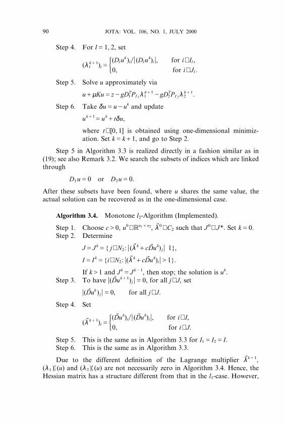
Example 4.3. The true and noisy images (δG1) are given in Fig. 4(top).

Example 4.4. The true and noisy images (δG1) are given in Fig. 4(bottom).

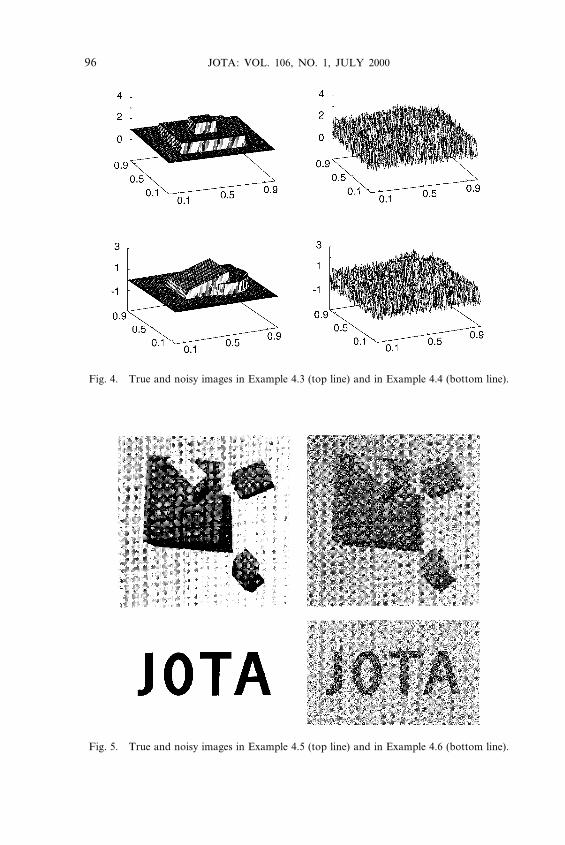
Example 4.5. The true and noisy images are given in Fig. 5 (top). Thesize of the image is 512B512 pixels. The (grey level values of the) true imagewas first scaled to the interval [0, 1]; after that, 50% of noise was added (δG0.5).

JOTA: VOL. 106, NO. 1, JULY 200096

Fig. 4. True and noisy images in Example 4.3 (top line) and in Example 4.4 (bottom line).

Fig. 5. True and noisy images in Example 4.5 (top line) and in Example 4.6 (bottom line).

JOTA: VOL. 106, NO. 1, JULY 2000 97

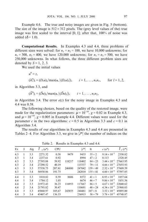
Example 4.6. The true and noisy images are given in Fig. 5 (bottom).The size of the image is 512B312 pixels. The (grey level values of the) trueimage was first scaled to the interval [0, 1]; after that, 100% of noise wasadded (δG1.0).

Computational Results. In Examples 4.3 and 4.4, three problems ofdifferent sizes were solved: for n1Gn2G100, we have 10,000 unknowns; forn1G300, n2G400, we have 120,000 unknowns; for n1Gn2G500, we have250,000 unknowns. In what follows, the three different problem sizes aredenoted by SG1, 2, 3.

We used the initial values

u0Gz,

(λ0l )iG(Dlu)iymax((, u (Dlu)i u), iG1, . . . , n1n2 , for lG1, 2,

in Algorithm 3.3, and

(λ≈0)iG(D≈u)iymax((, u (D≈u)i u), iG1, . . . , n1n2 ,

in Algorithm 3.4. The error e(z) for the noisy image in Examples 4.3 and4.4 was 0.58.

The following choices, based on the quality of the restored image, weremade for the regularization parameters: µG10−10, gG0.02 in Example 4.3,and µG10−10, gG0.005 in Example 4.4. Different values were used for theparameter c in the two algorithms: cG0.5 in Algorithm 3.3 and cG0.1 inAlgorithm 3.4.

The results of our algorithms in Examples 4.3 and 4.4 are presented inTables 2–4. For Algorithm 3.3, we give in uJ*u the number of indices on the

Table 2. Results in Examples 4.3 and 4.4.

Ex S Alg T h (u*) CPU uJ*u It e (u*) Th (z*)

4.3 1 3.3 2271.32 0.58 9479 9433 35C2 9.14B10−2 2330.824.3 1 3.4 2237.61 0.92 8994 47C2 0.113 2328.454.3 2 3.3 27395.88 59.92 118217 118402 84C23 3.44B10−2 27663.954.3 2 3.4 27290.52 40.19 115337 79C11 4.66B10−2 27655.934.3 3 3.3 57538.75 207.81 246880 247042 139C49 2.32B10−2 57609.594.3 3 3.4 56930.86 191.75 242010 135C41 4.60B10−2 57597.85

4.4 1 3.3 1810.82 0.59 8606 8572 41C1 8.95B10−2 1857.644.4 1 3.4 1784.12 1.05 6674 46C7 9.86B10−2 1851.564.4 2 3.3 21972.43 36.23 116953 117667 86C5 4.67B10−2 22040.624.4 2 3.4 21795.82 30.47 110691 48C24 4.34B10−2 21968.034.4 3 3.3 45860.97 105.67 243855 244481 107C8 3.52B10−2 45895.004.4 3 3.4 45407.47 136.33 236915 58C79 3.78B10−2 45748.87

JOTA: VOL. 106, NO. 1, JULY 200098

Table 3. Nested Algorithms in Examples 4.3 and 4.4.

Ex S Alg CPU uJ*u It e (u*)

4.3 2 N3.3 15.79 117389 117759 24C1, 8C1, 1C30 1.19B10−2

4.3 2 N3.4 20.25 113996 11C2, 27C10, 11C28 4.78B10−2

4.3 3 N3.3 39.04 246370 247,100 26C9, 29C3, 31C1 1.53B10−2

4.3 3 N3.4 56.98 242862 34C4, 7C19, 51C3 3.64B10−2

4.4 2 N3.3 18.08 115636 117542 19C1, 39C1, 37C1 3.88B10−2

4.4 2 N3.4 34.01 109867 3C20, 1C38, 67C1 5.39B10−2

4.4 3 N3.3 68.66 243398 245628 26C2, 40C15, 55C7 3.72B10−2

4.4 3 N3.4 133.20 237750 2C31, 57C8, 119C8 4.22B10−2

Table 4. Algorithm N3.3 for 20 and 10 iterations per level.

Ex S Alg CPU It e(u*)

4.3 2 N3.3 2.85 10C8C3 5.72B10−2

4.3 2 N3.3 10.92 20C2, 17C7, 20C2 1.19B10−2

4.3 3 N3.3 12.26 10C9C10 4.21B10−2

4.3 3 N3.3 46.87 20C3, 20C12, 20C20 2.03B10−2

4.4 2 N3.3 4.73 10C10C10 4.90B10−2

4.4 2 N3.3 18.21 19C1, 20C11, 20C20 3.88B10−2

4.4 3 N3.3 11.76 10C10C10 5.16B10−2

4.4 3 N3.3 46.62 20C7, 20C20, 20C20 3.86B10−2

final active sets J*1 and J*2 . By Th , we denote the cost functionals T2 andT3 . The results of Algorithms 3.3 and 3.4 are given in Table 2 and theresults of nested versions of the algorithms are given in Table 3. In thenested experiments, we applied the following strategy, which is further dis-cussed in Section 4.4 (ii). The values of the parameter g given above wereused at coarser levels; the value was decreased to gG0.001 at the finestlevel. Plots of the results of Algorithms 3.3 and 3.4 are given in Figs. 6 and7, where the plot on the left corresponds to Algorithm 3.3 and the plot onthe right corresponds to Algorithm 3.4. Plots of the results of AlgorithmN3.3 are given in Fig. 8 (top line).

Examples 4.5 and 4.6 involve grey scale images. In Fig. 9, the resultsof Algorithm 3.3 are given. In Example 4.5, we chose gG5 · 10−4; inExample 4.6, we chose gG3 · 10−3; the other parameters had the same valuesas above. In Example 4.5, the number of iterations was 103 and the elapsedCPU time was 197 seconds; in Example 4.6, the algorithm took 133 iter-ations and the elapsed CPU time was 173 seconds.

4.4. Conclusions from Numerical Experiments.

(i) Closeness of the Obtained Result u* to the True Image. We man-aged to restore the original images reasonably well; see Figs. 2–9. Still, there

JOTA: VOL. 106, NO. 1, JULY 2000 99

Fig. 6. Restored images in Example 4.3 for SG1 (100B100) (top line) and SG3 (500B500)(bottom line).

Fig. 7. Restored images in Example 4.4 for SG1 (100B100) (top line) and SG3 (500B500)(bottom line).

JOTA: VOL. 106, NO. 1, JULY 2000100

Fig. 8. Results of Algorithm N3.3 for SG3 (top line). Algorithm N3.3 with 10 iterations atall levels for cG0.5 (bottom line).

Fig. 9. Results of Algorithm 3.3 in Examples 4.5 and 4.6.

JOTA: VOL. 106, NO. 1, JULY 2000 101

was some error between obtained results and true images. However, thecomputed values of the cost functional were smaller than the correspondingvalues for the true images. From this, we conclude that the differencebetween the original image and the obtained result is partly caused by theoriginal formulation of the problem and not by unsuccessful minimization,for example. If the original formulation includes more information (givenstandard deviation, for example), a better value of g can be obtained, andthis improves the quality of the solution.

(ii) Comparison of Different Modifications of the Basic Active-SetAlgorithm. When testing nested iterations algorithms, we tried both ways,the bilinear restriction and the trivial injection, to determine the coarserproblems. Bilinear restriction gave better results, which are presented inTable 3. Since the nested iterations algorithm gives a smooth initial guess,we are able to decrease the value of the regularization parameter g at thelast level. Hence, we restrict less the variation of the image and try to betterrecover the true shape.

Algorithm N3.3 works well. It gives small errors e(u*) and is consider-ably faster than Algorithm 3.3. Algorithm N3.4 seems to work in Example4.3 where the true image is piecewise constant, but the results in Example4.4 are not as good. The errors e(u*) are slightly bigger and Algorithm N3.4is not at all faster than Algorithm 3.4.

Finally, we note that the modifications in the implemented algorithms,namely the usage of two different values of c and nested iterations typetechnique, were convergent in all examples.

(iii) Scalability and Efficiency. Figure 10 shows how the elapsed CPUtime, number of iterations, and size of the problem relate to each other inExamples 4.3 and 4.4. In the figures, the plot on the left corresponds toAlgorithm 3.3; the plot on the right corresponds to Algorithm 3.4. Withsome exceptions, there seems to be a mildly linear growth in number ofiterations and elapsed CPU time. Note that the direct inner iteration is inany case an O (N)-operation. We recall that an approximate Hessian matrixwas used in l2-algorithms. Still the number of iterations for the l2-algorithmcompared to the l1-algorithm is satisfactory in Fig. 10.

Using nested iterations in Algorithm 3.3 decreases considerably theelapsed CPU time and number of iterations; see Table 3. Actually, alreadyten iterations of Algorithm N3.3 at all levels gives satisfactory results witha very low CPU time. The results in Examples 4.3 and 4.4 for SG3 are givenin Fig. 8. In these results, a larger error level e(u*) remains. By allowing 20iterations at each level and using two values of c, also the error level is thesame as with the full algorithm; see Table 4. This implies that, if the primaryinterest is on the edge detection, it is not necessary to solve precisely theoriginal optimization problem. Moreover, after removing noise using an

JOTA: VOL. 106, NO. 1, JULY 2000102

Fig

.10

.E

laps

edC

PU

tim

ein

seco

nds

and

num

ber

ofiter

atio

nsin

Exa

mpl

e4.

3(t

oplin

e)an

din

Exa

mpl

e4.

4(b

otto

mlin

e).

JOTA: VOL. 106, NO. 1, JULY 2000 103

active-set algorithm, the edge detection can be focused into the inactive setonly or the union of the inactive sets in the l1-algorithms.

The efficiency of the implicit active-set methods compared to theexplicit Uzawa method can be seen in Example 4.2 where, for nG5000, theelapsed CPU time for the active-set method was 0.4 seconds, whereas theUzawa algorithm took 43 minutes. The monotone direct method was twiceas fast as the nonmonotone penalty method already in 1D. In the nonmono-tone algorithm, a linear system with tridiagonal matrix is solved in everyiteration. In 2D, the bandwidth of the system matrix arising from the pen-alty method grows to n2 . Thus, compared to our direct method with O (N )operations, the number of operations for solving this linear system usinge.g. the Cholesky method is of order O (n2

2N )≈O (N2) for n1≈n2 . Moreover,there is a similar, substantial difference between the storage requirements aswell.

(iv) Role of the Parameter c in Active-Set Algorithms. It is shownin Ref. 1 that the basic active-set algorithms without linearization becomeindependent of c after the first iteration. However, due to the explicit updateof the Lagrange multiplier in Step 4 of Algorithms 3.1 to 3.4, this is notvalid for the implemented algorithms. Decreasing the value of c makes theactive set J* too big and the result is not satisfactory. Increasing the valueof c does not have a remarkable influence on the results, but it increasesconsiderably the number of iterations needed. Hence, we utilize this obser-vation both in the initial choices cG0.5 and cG0.1 and in the two-stepprocedure described earlier.

(v) Values of Different Parameters and Sensitivity of Results. Duringthese experiments (various examples using the given algorithms and differ-ent amount of unknowns), after fixing the values of the parameters in thebeginning, the only parameter we had to adjust was the regularization par-ameter g. Thus, using the proposed values, neither the dimension of theproblem nor the problem itself has effect on the choices of parameters otherthan g.

5. Conclusions

Active-set methods for solving the nonsmooth, convex optimizationproblems that arise in image restoration were studied through numericalexperiments. Implemented nonmonotone and monotone active-set algo-rithms for solving the one-dimensional image restoration problem as wellas monotone algorithms with a modified regularization for solving the two-dimensional problems were given. For µ[h2, a novel, direct way for solvingthe constrained optimization problem that appears in the inner iteration ofthe monotone algorithms was described.

JOTA: VOL. 106, NO. 1, JULY 2000104

The performance of the given algorithms was tested through severalnumerical examples. In all the examples, there was a considerable amountof noise. However, we managed to restore the original images reasonablywell in a computationally efficient manner. The l1-Algorithm N3.3 withnested iterations turned out to be the most attractive of the tested methods,because of its efficiency and restoration capability.

References

1. KARKKAINEN, T., and MAJAVA, K., Nonmonotone and Monotone Active SetMethods for Image Restoration, Part 1: Convergence Analysis, Journal of Optim-ization Theory and Applications, Vol. 106, pp. 61–80, 2000.

2. RUDIN, L. I., OSHER, S., and FATEMI, E., Nonlinear Total-Variation BasedNoise Removal Algorithms, Physica D, Vol. 60, pp. 259–268, 1992.

3. VOGEL, C. R., and OMAN, M. E., Iterative Methods for Total-Variation Denois-ing, SIAM Journal on Scientific Computing, Vol. 17, pp. 227–238, 1996.

4. VOGEL, C. R., and OMAN, M. E., Fast, Robust Total-Variation Based Recon-struction of Noisy, Blurred Images, IEEE Transactions on Image Processing,Vol. 7, pp. 813–824, 1998.

5. CHAN, T., GOLUB, G., and MULET, P., A Nonlinear Primal–Dual Methodfor Total-Variation Based Image Restoration, SIAM Journal on Scientific Com-puting, Vol. 20, pp. 1964–1977, 1999.

6. CHAMBOLLE, A., and LIONS, P. L., Image Recovery via Total-Variation Minim-ization and Related Problems, Numerische Mathematik, Vol. 76, pp. 167–188,1997.

7. ITO, K., and KUNISCH, K., An Active Set Strategy Based on the AugmentedLagrangian Formulation for Image Restoration, Mathematical Modelling andNumerical Analysis, Vol. 33, pp. 1–21, 1999.

8. MAJAVA, K., Kohinanpoisto Lagrange-Menetelmilla, MS Thesis, University ofJyvaskyla, 1998 (in Finnish).

9. KARKKAINEN, T., and MAJAVA, K., Nonmonotone and Monotone Active SetMethods for Image Restoration, Technical Report B9y1999, Department ofMathematical Information Technology, University of Jyvaskyla, 1999.

10. CASAS, E., KUNISCH, K., and POLA, C., Regularization by Functions of BoundedVariation and Applications to Image Enhancement, Applied Mathematics andOptimization, Vol. 40, pp. 229–257, 1999.

11. BERTSEKAS, D. P., Constrained Optimization and Lagrange Multiplier Methods,Academic Press, New York, NY, 1982.

12. HACKBUSCH, W., Multigrid Methods and Applications, Springer Series in Com-putational Mathematics, Springer Verlag, Berlin, Germany, 1985.

13. ITO, K., and KUNISCH, K., Augmented Lagrangian Formulation of Nonsmooth,Convex Optimization in Hilbert Spaces, Control of Partial Differential Equationsand Applications, Edited by E. Casas, Lecture Notes in Pure and Applied Math-ematics, Marcel Dekker, New York, NY, Vol. 174, pp. 107–117, 1995.

JOTA: VOL. 106, NO. 1, JULY 2000 105

14. EKELAND, I., and TEMAM, R., Convex Analysis and Variational Problems, Stud-ies in Mathematics and Its Applications, North-Holland, Amsterdam, Holland,Vol. 1, 1976.

15. GLOWINSKI, R., LIONS, J. L., and TREMOLIERES, R., Numerical Analysis ofVariational Inequalities, North-Holland, Amsterdam, Holland, 1981.