Computational Intelligence, Volume 22, Number 1, 2006 NONMONOTONIC LOGIC AND STATISTICAL INFERENCE ∗ HENRY E. KYBURG,JR. Computer Science and Philosophy, University of Rochester, Rochester, NY 14627, USA; Institute for Human and Machine Cognition, 40 South Alcaniz Street, Pensacola, FL 32502, USA CHOH MAN TENG Institute for Human and Machine Cognition, 40 South Alcaniz Street, Pensacola, FL 32502, USA Classical statistical inference is nonmonotonic: obtaining more evidence or obtaining more knowledge about the evidence one has can lead to the replacement of one statistical conclusion by another, or the complete withdrawal of the original conclusion. While it has long been argued that not all nonmonotonic inference can be accounted for in terms of relative frequencies or objective probabilities, there is no doubt that much nonmonotonic inference can be accounted for in this way. Here we seek to explore the close connection between classical statistical inference and default logic, treating statistical inference within the framework of default logic, and showing that nonmonotonic logic in general, and default logic in particular, needs to take account of certain features of statistical inference. Default logic must take account of statistics, but at the same time statistics can throw light on problematic cases of default inference. Key words: nonmonotonic logic, default logic, probability, statistical inference, thresholding. 1. INTRODUCTION It is natural to think of the grounds for the defaults studied by Reiter (1980) and others (e.g., Lukaszewicz 1988; Brewka 1991; Gelfond et al. 1991; Delgrande, Schaub, and Jackson 1994; Mikitiuk and Truszczy´ nski 1995) as lying in what we know of relative frequencies in the world: practically all birds fly, practically all husbands and wives live in the same city. But there are those who have denied that high-relative frequency is necessary for default reasoning (e.g., McCarthy 1986). Our concern is not with this issue, but with a related one: classical statistical inference. Classical statistical inference is based on the idea that samples are somehow typical of the populations from which they are drawn. This is true of most samples. But the operative principles of statistical inference are somewhat different: they have to do, not with exploiting typicality or high frequencies directly, but with the control of frequencies of error (Mayo 1996). Not only do the terms in which classical statistical inference is conducted conform closely to the framework of default inference, but we believe the distinction between the prerequisite of an inference, the premise without which the inference cannot take place, and the justifications of the inference, the statements that must not be believed if the inference is to go through, is a distinction that can throw considerable light on the statistical inference (Kyburg and Teng 1999). On the other hand, while some default inferences seem uncontroversial (Tweety flies comes to mind), there are other default inferences, or groups of default inferences that seem more controversial. For example, a person may be both a Quaker (and thus, typically, a pacifist) and a Republican (and thus, typically, a hawk). We shall claim that considerations that guide our choice of reference classes in probability and statistics may also prove valuable in sorting out these difficult sets of default inferences. First steps toward this problem—the problem of approaching statistical inference as a kind of default inference—were taken in Kyburg and Teng (1999), but the issue was not ∗ This material is based upon work supported by NSF IIS 0328849, NASA NNA04CK88A, and ONR N00014-03-1-0516. C 2006 Blackwell Publishing, 350 Main Street, Malden, MA 02148, USA, and 9600 Garsington Road, Oxford OX4 2DQ, UK.

Nonmonotiic Logic
Dec 21, 2015
monotonicity and logic
Welcome message from author
This document is posted to help you gain knowledge. Please leave a comment to let me know what you think about it! Share it to your friends and learn new things together.
Transcript
Computational Intelligence, Volume 22, Number 1, 2006
NONMONOTONIC LOGIC AND STATISTICAL INFERENCE∗
HENRY E. KYBURG, JR.Computer Science and Philosophy, University of Rochester, Rochester, NY 14627, USA; Institute
for Human and Machine Cognition, 40 South Alcaniz Street, Pensacola, FL 32502, USA
CHOH MAN TENG
Institute for Human and Machine Cognition, 40 South Alcaniz Street, Pensacola, FL 32502, USA
Classical statistical inference is nonmonotonic: obtaining more evidence or obtaining more knowledge aboutthe evidence one has can lead to the replacement of one statistical conclusion by another, or the complete withdrawalof the original conclusion. While it has long been argued that not all nonmonotonic inference can be accounted forin terms of relative frequencies or objective probabilities, there is no doubt that much nonmonotonic inference canbe accounted for in this way. Here we seek to explore the close connection between classical statistical inference anddefault logic, treating statistical inference within the framework of default logic, and showing that nonmonotoniclogic in general, and default logic in particular, needs to take account of certain features of statistical inference.Default logic must take account of statistics, but at the same time statistics can throw light on problematic cases ofdefault inference.
Key words: nonmonotonic logic, default logic, probability, statistical inference, thresholding.
1. INTRODUCTION
It is natural to think of the grounds for the defaults studied by Reiter (1980) and others(e.g., Lukaszewicz 1988; Brewka 1991; Gelfond et al. 1991; Delgrande, Schaub, and Jackson1994; Mikitiuk and Truszczynski 1995) as lying in what we know of relative frequencies inthe world: practically all birds fly, practically all husbands and wives live in the same city.But there are those who have denied that high-relative frequency is necessary for defaultreasoning (e.g., McCarthy 1986). Our concern is not with this issue, but with a related one:classical statistical inference. Classical statistical inference is based on the idea that samplesare somehow typical of the populations from which they are drawn. This is true of mostsamples. But the operative principles of statistical inference are somewhat different: theyhave to do, not with exploiting typicality or high frequencies directly, but with the control offrequencies of error (Mayo 1996).
Not only do the terms in which classical statistical inference is conducted conformclosely to the framework of default inference, but we believe the distinction between theprerequisite of an inference, the premise without which the inference cannot take place, andthe justifications of the inference, the statements that must not be believed if the inferenceis to go through, is a distinction that can throw considerable light on the statistical inference(Kyburg and Teng 1999).
On the other hand, while some default inferences seem uncontroversial (Tweety fliescomes to mind), there are other default inferences, or groups of default inferences that seemmore controversial. For example, a person may be both a Quaker (and thus, typically, apacifist) and a Republican (and thus, typically, a hawk). We shall claim that considerationsthat guide our choice of reference classes in probability and statistics may also prove valuablein sorting out these difficult sets of default inferences.
First steps toward this problem—the problem of approaching statistical inference as akind of default inference—were taken in Kyburg and Teng (1999), but the issue was not
∗This material is based upon work supported by NSF IIS 0328849, NASA NNA04CK88A, and ONR N00014-03-1-0516.
C© 2006 Blackwell Publishing, 350 Main Street, Malden, MA 02148, USA, and 9600 Garsington Road, Oxford OX4 2DQ, UK.

NONMONOTONIC LOGIC AND STATISTICAL INFERENCE 27
treated in depth there. The role of statistical considerations in default inference, similarly,was only touched upon in Kyburg and Teng (2001).
2. STATISTICAL INFERENCE
Statistical inference comes in many forms. Most of these forms require something in theway of background knowledge, though it is interesting that confidence interval inference toclass ratios arguably need not depend on empirical assumptions. We take statistical inferenceas involving the tentative acceptance (or rejection) of a statistical hypothesis, or of somestatement equivalent to a statistical hypothesis. For example, measurement is often takento yield an interval within which a physical quantity is taken to fall. But since the truevalue of that quantity is the mean of the (hypothetical) unbounded population of adjustedmeasurements of that quantity, to say that a quantity lies in an interval is to say that the meanof an unbounded population of measurements lies in that interval. Even measurement can beconstrued as statistical inference.
Much of science uses statistical inference in a more transparent way. According to somewriters (Chow 1996), most scientific inference can be construed in terms of significancetesting. While we do not accept that thesis, we do agree that significance testing plays animportant role in many branches of science. Hypothesis testing that can be seen as the foun-dation of statistical inference in the prevalent classical British–American school (Lehmann1959) can be extended in many ways, and can, in particular, be taken as a foundation forconfidence interval analysis. Finally, there is Bayesian statistics. Bayesian statistics is oftenso-called because it allows us to take account of background knowledge, which is more exten-sive than is ordinarily dealt with by classical statistics, and thereby allows the use of Bayes’theorem in ways that would be prohibited in classical terms. It is also, sometimes, construedas more extreme—as denying that statistical hypotheses are ever legitimately “accepted” andinsisting that all we can do (and all we ought to do) on the basis of experience is to updateour probabilities, including the probabilities we assign to statistical hypotheses. This latterpossibility is one we shall not focus on, since it does not seem to us to involve nonmono-tonicity. When one updates probabilities by conditioning, the “new” probability is based onthe same probability function with which one started: P(A | B ) = P(A ∧ B )/P(B ). No newfunction need be introduced; we do not withdraw the results of previous inference. To besure, the agent’s confidence in A changes with the observation of B, and changes again withthe further observation of C. But what we infer on the basis of the observation B is P(A | B)and not P(A); what we infer on the basis of the further observation C is P(A | B ∧ C ), not yetanother value of P(A).
2.1. Significance Testing
The guiding idea behind significance testing is the control of error (Fisher 1971;Chapter 2). A classic example of simple significance testing is this: Suppose that hypothesisH0, the null hypothesis, asserts that the relative frequency of defective toasters manufacturedon a certain production line is less than 10%. We design a test for this hypothesis; for example,we decide to examine n toasters from the line and to reject H0 if more than k are defective.As is characteristic of significance tests, we arrive at no conclusion if k or less toasters inour sample are defective: we simply fail to reject H0. We may ask, as thoughtful statisticianshave, what it means to reject a hypothesis. To reject H0 is to perform a positive act; it isto abandon suspension of belief; it is to accept ¬H0, i.e., it is to accept that at least 10%

28 COMPUTATIONAL INTELLIGENCE
of the toasters produced by that line are defective. To fail to reject H0, on the other hand,calls for no action at all; we remain completely agnostic about the frequency of defectivetoasters.
The significance test is characterized as follows: The size of the test, α, is the maximumlong run chance of falsely rejecting the hypothesis under test, H0, i.e., the long run relativefrequency of obtaining k or more defective toasters out of n, given that less than 10% in generalare defective. Given that H0 is true, we can calculate this maximum long run frequency oferror precisely.
This is the “before test” analysis of the significance test of H0. This does not end thedesign of the test. We must stipulate how these n toasters are to be selected from thoseproduced (they must be selected in such a way that the long run frequency of error appliesto the sample we have selected), and we must also specify the standard according to whichthey will be judged defective or not.
Finally, we must actually perform the sampling and testing, and draw the conclusion,“Reject H0” or “Do not reject H0,” according as we observe more than k defectives in oursample or not.
We point out two things. First, if H0 is rejected, this is really, and not just metaphorically,inference. When we “reject” H0, we accept ¬H0. We stop the production line and look forthe source of the excess defects. If H0 is the “no effect” hypothesis for a cold remedy, wedevise more and more sensitive tests; we pursue the development of the remedy, at least fora while.
Of course, if we “fail to reject” H0, we have inferred nothing. The possibilities are justwhat they were before our test.
The second thing to note is that this inference, when it occurs, is nonmonotonic: furtherpremises (more data) could lead to our retracting the conclusion ¬H0. For example, we couldlook at a larger sample, and note a smaller fraction of defectives. But there are also less directgrounds we could have for rejecting the conclusion. For example, we might learn that whenthe production line first starts up there are a large number of defects, until the machinery getswarmed up, and that our sample was taken from the start of the line. Or we might learn thatthe sample was taken and analyzed by an engineer who is notoriously careless.
In the process of testing, there are a number of conditions we must think about; we willcome back to them in Section 5, after a brief review of evidential probability and default logic,since these conditions are best construed, we will argue, as “justifications” of the relevantstatistical default rules.
2.2. Hypothesis Testing
In hypothesis testing, we take account not only of the error of falsely rejecting a hypothesisthat is true (the possibility of false rejection in significance testing) but we also take accountof the error of failing to reject a hypothesis that is false. The first of these errors is Type Ierror; it is also called the size of a test, and often denoted by α. The second of these errors,called error of Type II, is often denoted by β; 1 − β is the power of a test.
We illustrate these ideas with a simple example, in which we test the hypothesis H0 that10% of the toasters in a shipment are defective against the hypothesis H1 that 60% of thetoasters are defective. We look at a sample of n. There are many possibilities for this sample,but for present purposes we can ignore the order in which the defective toasters appear. Thus,we focus on the n + 1 points in the sample space corresponding to the number of possibledefective toasters in our sample.
Given the hypothesis under test, H0, we can calculate the proportion of samples that have0, 1, . . . , n defective toasters. If we want the size of our test to be 0.05, we want to be sure
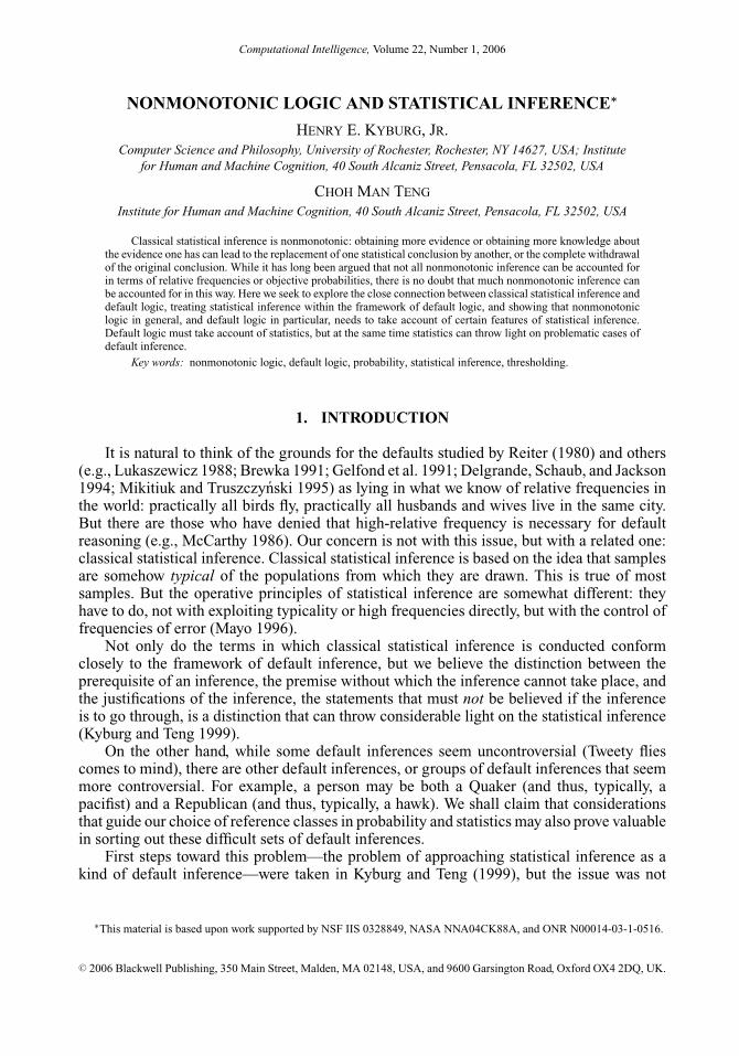
NONMONOTONIC LOGIC AND STATISTICAL INFERENCE 29
that we do not reject H0, given that it is true, in more than 5% of the cases. We will achievethis goal if we choose a value of k such that
∑i≤k(n
i )0.1i 0.9n−i is <0.05. That is easy: forn = 100, we could choose k = 0. The probability of error that we associate with this elementof the sample space is (100
0 )0.100.9100—a very small number indeed.But while this would give us excellent protection against falsely rejecting H0, we would
be led to accept the alternative hypothesis H1 far too infrequently. (We do not deal withthe possibility of suspending judgment; that would be a third alternative that would not addanything at this stage of our inquiry.) So what we want to do is to keep α at 0.05, and at thesame time maximize the chances of rejecting H0 when it is false. Just as we can calculate therelative frequency with which H0 will be falsely rejected, so we can calculate the frequencywith which it will erroneously fail to be rejected. We can do this because we are testing asimple hypothesis against a simple alternative. Suppose that the critical value of k is k0: if wefind k0 or more defects in our sample, we reject H0. Despite the fact that we have set this upas a test of one hypothesis against another, to reject one is not to be committed to the other:to reject H0 is to accept ¬H0, but not to accept H1, unless we have the disjunction H0 ∨ H1
as part of our background knowledge.To fail to reject H0 need not be to accept H0, and so, of course, need not be to reject
H1; nor, of course, is the rejection of H0 tantamount to the acceptance of H1. It may be, forexample, that when we control error of the first kind to be less than 0.05, our test may allowerror of the second kind to be 0.30—far too large to warrant acceptance of H1.
Again we emphasize, first, that when we accept ¬H0 we are performing a genuineinference. We send the shipment of toasters back, and we publish results, and we conductnew experiments. With the possible exception of the uncertainties involved, this is an inferencein the same sense as that which allows us to infer the velocity of a 1 gram bullet from theacceleration of a 10 kg block of wood into which it has been fired.
And second, this is a nonmonotonic inference. We may reinstate H0 if we examinethe whole shipment and find less than 10% defectives. Even the examination of a largersample might lead us to withdraw our conclusion. Learning that the sampling was done byan undercover agent of a competing supplier could also undo our acceptance of ¬H0.
2.3. Confidence Intervals
The simplest example of a confidence interval inference is measurement—say the mea-surement of a length. A method of measurement M is characterized by the distribution oferrors that it produces. In the best cases, the errors are known to be distributed approximatelynormally, with a mean of 0, and a well-established standard deviation d. The “true length” ofan object may be taken to be the mean of all possible measurements of it.
Let us apply method M to the measurement of an object o; suppose we obtain the resultm(o). Of course, we cannot conclude that the length of o is m(o); measurements, as we justnoted, are subject to error. Nor can we impose bounds on the possible value of the true lengthl(o) of o: given that the distribution of error is normal, an error of any finite magnitude ispossible. But noting that the true length of o is the expectation of measurements of it, we canconstrue inferring the true length as inferring that expectation—that is, making a statisticalinference. If M yields errors that are normal (0, d ), then measurements of o by this methodwill be distributed normally with mean equal to the true length l(o), and the same standarddeviation d.
Suppose that one chance in a hundred of error strikes us as secure enough. We cancalculate positive numbers δ1 and δ2 such that the result of measuring o will lie outside theinterval l(o) − δ1, l(o) + δ2 at most 1% of the time. We can find many such numbers, but if

30 COMPUTATIONAL INTELLIGENCE
we also impose the constraint that δ1 + δ2 be a minimum, we obtain a unique result. Often,as in this case, the interval will be symmetric: δ1 = δ2 = δ.
The problem, of course, is applying this analysis to the particular result m(o) we obtainedwhen we conducted our measurement. This is what we do, without fretting, and often withouteven thinking of it as statistical inference. If M is characterized by a standard deviation d,and we observe m(o), we infer (with confidence 0.99) that the true length of o, l(o), is in theinterval m(o) ± 2.58d.
What this means is a matter of some dispute. Many classical statisticians will insist thatwhat is characterized by the number 0.99 is the method M , and that all we can say of m(o)is that it is within a distance 2.58d of l(o) or that it is not. We shall argue later that thereis a sensible objective interpretation of probability according to which we can say that theprobability is 0.99 that l(o) ∈ m(o) ± 2.58d.
For present purposes the issue is not that this is statistical inference, but that it is inference.Having made the measurement, we conclude that o will fit in an opening that is m(o ) +2.58d wide. We conclude that it meets specification (or that it does not). We infer that thecombined length of this and another object o′, whose true length is l(o′), will be m(o ) + l(o′)±2.58d.
There is not much doubt that this is inference. Nor can there be much doubt that itis nonmonotonic. Even a second measurement would undermine the conclusion, since wewould be well advised to take the results of both measurements into account. We might alsoknow something relevant about the provenance of the object o that bears on its length. Or wemight get access to other measurements of o. It is only in the absence of other informationthat we infer that the true length of o is in the interval m(o ) ± 2.58d.
2.4. Inferring Relative Frequencies
These examples have involved premises—statements we take ourselves to know oraccept—as well as requiring that we not know or accept certain other things. There is aform of statistical inference, first formalized in 1932 (Clopper and Pearson 1934) that (ar-guably) requires no general statistical premises. Loosely speaking, since most samples froma finite population of which a proportion p of individuals are B represent the proportion ofitems that are B in that parent population, in the sense that the ratio of B’s in the sample isclose to p, we can infer from a sample something about this proportion. A bit less loosely(in fact quite precisely), given a sample size n, in which a number m of B’s occur, and givena confidence level, e.g., 0.99, we can compute upper and lower limits u(m/n ) and l(m/n )such that u(m/n ) − l(m/n ) is a minimum, and the claim that the proportion p of B’s in theparent population lies between these limits deserves at least that confidence. No assumptionsor approximations are involved—only inequalities. Although, it is frequently argued that thisnumber, 0.99, is not a probability, that argument is based on a particular interpretation ofprobability, and it is arguable from another, equally objective, point of view, that this numbercan be construed as a probability.
In any event, it is clear that this is an inference: to argue from a premise concerninga sample to a conclusion expressing a constraint on the relative frequency in the parentpopulation is an uncertain inference whose conclusion is supported but not entailed by itspremises. It is also abundantly clear that this inference is nonmonotonic. No doubt the reader’smind is already buzzing with possibilities that would undermine the inference. For example,we might already know what proportion of the population are B’s. We might obtain a largersample. We might know that the population in question comes from a set of populations inwhich the distribution of the frequency p of B is known.
NONMONOTONIC LOGIC AND STATISTICAL INFERENCE 31
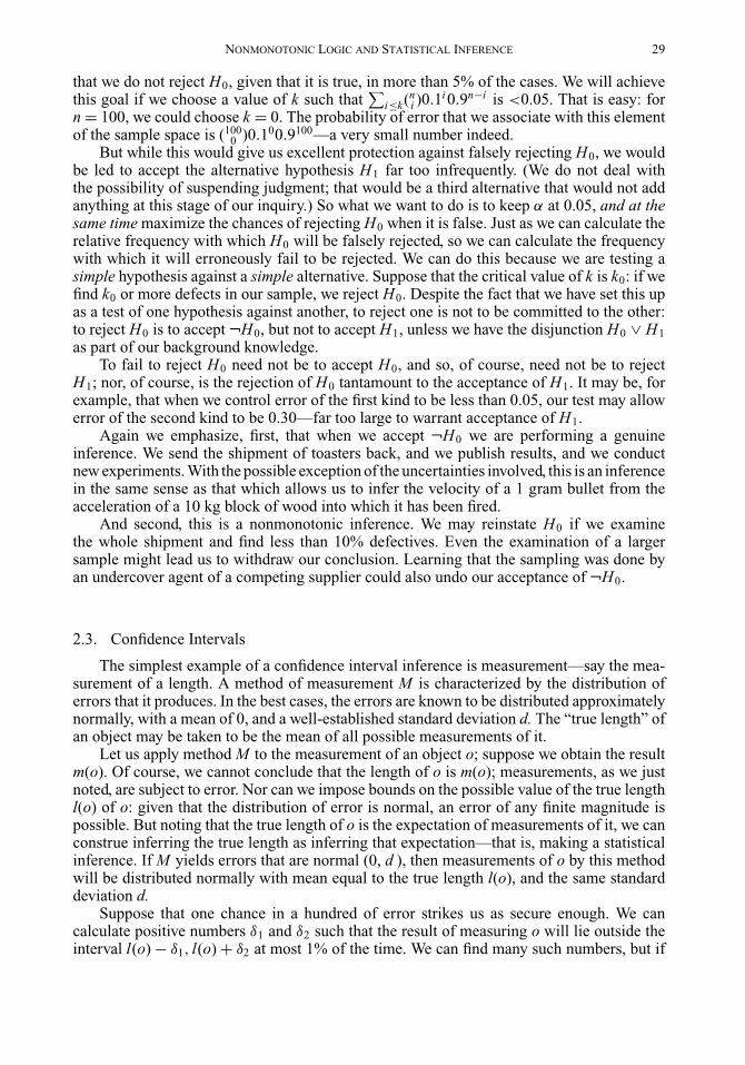
3. EVIDENTIAL PROBABILITY
We have already incurred the irritation (or worse) of classical statisticians by referring tothe “probabilities” of statistical hypotheses as possibly objective. We propose here to give avery brief sketch of evidential probability, an approach to probability that justifies this usage.
Probability is assigned to sentences relative to a body of knowledge and evidence, on thebasis of known approximate relative frequencies. Probabilities are therefore interval valued.The probability of a statement S, relative to a set of statements � constituting our evidenceand background knowledge, is the interval [p, q]—Prob(S, �) = [p, q]—and is objectivelydetermined as follows.
The frequency footing of any probability is a set of statements of the form %x(τ (x ), ρ(x ),p, q )1 which assert that the relative frequency of objects (tuples) satisfying the formula ρ thatalso satisfy the formula τ lies between p and q. There are many such statements we know; forexample, “%x(x lands heads, x is a toss of a coin, 0.45, 0.55),” including logically true onessuch as “%y(the proportion of A’s in y differs by less than k/(2
√n) from the proportion in B
in general, y is an n-membered subset of B’s, 1 − 1/k2, 1.0).” A sentence %x(τ (x ), ρ(x ), p,q ) is a candidate for the probability of a sentence S provided that for some term “α” of ourlanguage the sentences “τ (α) ≡ S” and “ρ(α)” are in �.
In general there will be many such statistical statements %x(τ (x ), ρ(x ), p, q ). Only threeprinciples are needed to resolve this problem. First, however, we must define the technicalrelation of conflict between statistical statements.
Definition 1. Given two intervals [p, q] and [r, s], we say that [p, q] is nested in [r, s] iffr ≤ p ≤ q ≤ s. The two intervals conflict iff neither is nested in the other. The cover of twointervals [p, q] and [r, s] is the interval [min(p, r ), max(q, s )].
Two statistical statements %x(τ (x ), ρ(x ), p, q ) and %x(τ ′(x ), ρ ′(x ), p′, q′) conflict if andonly if their associated intervals [p, q] and [p′, q′] conflict.
Note that conflicting intervals are not necessarily disjoint. They may overlap as long asneither is included entirely in the other.
Rule I
If two statistical statements conflict and the first is based on a marginal distribution whilethe second is based on the full joint distribution, ignore the first. This gives conditionalprobabilities pride of place when they conflict with the corresponding marginal probabilities.We will call this the principle of conditioning.
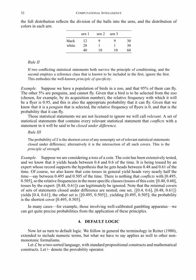
Example. Suppose we have 30 black and 30 white balls in a collection C. The relativefrequency of black balls among balls in C is 0.5, and this could serve as a probability that aspecific ball a in C is black. But if the members of C are divided into three urns, one of whichcontains 12 black balls and 28 white balls, and two of which each contains nine black ballsand one white ball, then if a is selected by a procedure that consists of (1) selecting an urn,and (2) selecting a ball from that urn, the relative frequency of black balls is 1/3(12/40) +1/3(9/10) + 1/3(9/10) = 0.70, and this is the appropriate probability that a, known to beselected in this way, is black. The marginal distribution is given by 30 black balls out of 60;
1These formulas are subject to constraints: they should exclude such predicates as “is an emerose” or “is grue” and theyshould mention the smallest justifiable intervals.
32 COMPUTATIONAL INTELLIGENCE
the full distribution reflects the division of the balls into the urns, and the distribution ofcolors in each urn.
urn 1 urn 2 urn 3
black 12 9 9 30white 28 1 1 30
40 10 10 60
Rule II
If two conflicting statistical statements both survive the principle of conditioning, and thesecond employs a reference class that is known to be included in the first, ignore the first.This embodies the well-known principle of specificity.
Example. Suppose we have a population of birds in a zoo, and that 95% of them can fly.The other 5% are penguins, and cannot fly. Given that a bird is to be selected from the zoo(chosen, for example, by its acquisition number), the relative frequency with which it willbe a flyer is 0.95, and this is also the appropriate probability that it can fly. Given that weknow that it is a penguin that is selected, the relative frequency of flyers is 0, and that is theprobability that it can fly.
Those statistical statements we are not licensed to ignore we will call relevant. A set ofstatistical statements that contains every relevant statistical statement that conflicts with astatement in it will be said to be closed under difference.
Rule III
The probability of S is the shortest cover of any nonempty set of relevant statistical statementsclosed under difference; alternatively it is the intersection of all such covers. This is theprinciple of strength.
Example. Suppose we are considering a toss of a coin. The coin has been extensively tested,and we know that it yields heads between 0.4 and 0.6 of the time. It is being tossed by anexpert whose record supports the hypothesis that he gets heads between 0.48 and 0.61 of thetime. Of course, we also know that coin tosses in general yield heads very nearly half thetime—say between 0.495 and 0.505 of the time. There is nothing that conflicts with [0.495,0.505], so the relative frequencies in the more specific classes (tosses of this coin: [0.40, 0.60],tosses by the expert: [0.48, 0.61]) can legitimately be ignored. Note that the minimal coversof sets of statements closed under difference are nested; one set, {[0.4, 0.6], [0.48, 0.61]}yields [0.4, 0.61]; the other set is {[0.495, 0.505]}, yielding [0.495, 0.505]; the probabilityis the shortest cover [0.495, 0.505].
In many cases—for example, those involving well-calibrated gambling apparatus—wecan get quite precise probabilities from the application of these principles.
4. DEFAULT LOGIC
Now let us turn to default logic. We follow in general the terminology in Reiter (1980),extended to include numeric terms, but what we have to say applies as well to other non-monotonic formalisms.
LetL be a two-sorted language, with standard propositional constructs and mathematicalconstructs. Let � denote the provability operator.

NONMONOTONIC LOGIC AND STATISTICAL INFERENCE 33
Definition 2. A default rule d is an expression of the form
α : β1, . . . , βn
γ,
where α, β1, . . . , βn, γ ∈ L. We call α the prerequisite, β1, . . . , βn the justifications, and γthe consequent of the default rule d. A default rule is normal if it is of the form α:γ
γ, and
seminormal if it is of the form α:β∧γ
γ.
A default theory is an ordered pair 〈F, D〉, where F is a set of sentences in L and D isa set of default rules.
Loosely speaking, a default rule α:β1,...,βn
γconveys the idea that if α is accepted, and
none of ¬β1, . . . ,¬βn are accepted, then by default we may assert γ . For a default theory=〈F, D〉, the known facts constitute F, and a theory extended from F by applying the defaultrules in D is known as an extension of , defined formally via a fixed point formulation.
Definition 3. Let = 〈F, D〉 be a default theory and E∗ be a set of sentences in L. LetE0 = F, and for i ≥ 0,
Ei+1 = {φ | Ei � φ}⋃ ⎧⎪⎪⎨⎪⎪⎩
γ
∣∣∣∣ α:β1,...,βn
γ∈ D,
α ∈ Ei ,
and ¬β1, . . . , ¬βn �∈ E∗
⎫⎪⎪⎬⎪⎪⎭The set of sentences E∗ is an extension of iff E∗ = ⋃
0≤i≤∞ Ei .
Basically, a default extension contains the set of given facts, is deductively closed, and alldefault rules that can be applied in the extension have been applied. In addition, an extensionhas to be minimal, that is, every sentence in an extension is either a fact or a consequent ofan applied default rule, or a deductive consequence of some combination of the two.
A default rule α:β1,...,βn
γcan be applied to conclude the consequent γ when the conditions
associated with its prerequisite α and justifications β1, . . . , βn are satisfied. The prerequisitecondition α is satisfied by showing that α is “present,” and each of the justification conditionsβ i is satisfied by showing that ¬β i is “absent.” Note that ¬β i is “absent” does not implyautomatically that β i is accepted. It merely means that there is no “hard proof ” that β i isfalse.
In the classical logic framework, the presence or absence of a formula is determinedby the deductive provability: α is “present” if α is provable from a set of sentences, and¬β i is “absent” if ¬β i is not provable from the same set of sentences. However, logicalprovability need not be the only way to determine whether a formula is “present” or “absent.”In particular, formulas obtained by the application of default rules may qualify as being“present.” This is particularly important in the current context, as we will see when weexamine the justifications for statistical inference.
5. STATISTICAL INFERENCE AS DEFAULT INFERENCE
“Assumptions” (or “presuppositions”) are sometimes invoked in statistical inference. Anexample is the “Simple Random Sampling” assumption (Moore 1979) often mentioned, andconstrued as the claim that each equinumerous subset of a population has the same probability
34 COMPUTATIONAL INTELLIGENCE
of being drawn. According to this assumption, every sample must have the same chance ofbeing chosen; but usually we know that that is false: Samples remote in space or time haveno chance of being selected.
We cannot choose a sample of trout by a method that will with equal probability selectevery subset of the set of all trout, here or there, past or present, with equal frequency. Yet,the population whose parameter we wish to evaluate may be precisely the set of all trout,here and there, past and present.
This is also true of the “sampling assumption” mentioned by Cramer (1951, p. 324)and also by Baird (1992, p. 31) which requires that each element in the domain has anequal probability of being selected.2 We cannot, therefore, take simple random sampling asa premise or a prerequisite of our statistical argument. We not only have no reason to acceptit, but, usually, some reasons for denying it.
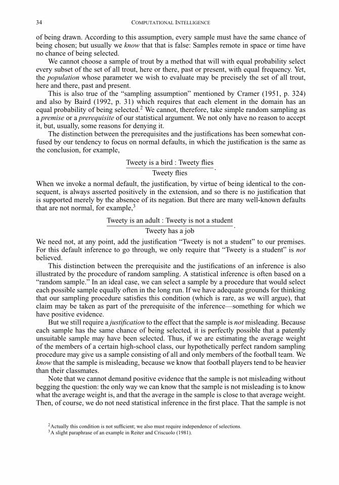
The distinction between the prerequisites and the justifications has been somewhat con-fused by our tendency to focus on normal defaults, in which the justification is the same asthe conclusion, for example,
Tweety is a bird : Tweety flies
Tweety flies.
When we invoke a normal default, the justification, by virtue of being identical to the con-sequent, is always asserted positively in the extension, and so there is no justification thatis supported merely by the absence of its negation. But there are many well-known defaultsthat are not normal, for example,3
Tweety is an adult : Tweety is not a student
Tweety has a job.
We need not, at any point, add the justification “Tweety is not a student” to our premises.For this default inference to go through, we only require that “Tweety is a student” is notbelieved.
This distinction between the prerequisite and the justifications of an inference is alsoillustrated by the procedure of random sampling. A statistical inference is often based on a“random sample.” In an ideal case, we can select a sample by a procedure that would selecteach possible sample equally often in the long run. If we have adequate grounds for thinkingthat our sampling procedure satisfies this condition (which is rare, as we will argue), thatclaim may be taken as part of the prerequisite of the inference—something for which wehave positive evidence.
But we still require a justification to the effect that the sample is not misleading. Becauseeach sample has the same chance of being selected, it is perfectly possible that a patentlyunsuitable sample may have been selected. Thus, if we are estimating the average weightof the members of a certain high-school class, our hypothetically perfect random samplingprocedure may give us a sample consisting of all and only members of the football team. Weknow that the sample is misleading, because we know that football players tend to be heavierthan their classmates.
Note that we cannot demand positive evidence that the sample is not misleading withoutbegging the question: the only way we can know that the sample is not misleading is to knowwhat the average weight is, and that the average in the sample is close to that average weight.Then, of course, we do not need statistical inference in the first place. That the sample is not
2Actually this condition is not sufficient; we also must require independence of selections.3A slight paraphrase of an example in Reiter and Criscuolo (1981).
NONMONOTONIC LOGIC AND STATISTICAL INFERENCE 35
misleading is a justification of the inference because we can have evidence that it is false (byknowing how the sample is misleading), while we cannot ordinarily have direct evidence thatit is true.4
What we can demand as a prerequisite is that the sample be obtained by a procedurethat conforms to good statistical practice. This will not guarantee that the sample is notmisleading—even perfect randomization would not guarantee that—but is as much as wecan ask as a prerequisite. The arguments go through anyway, and justifiably so. Our lack ofknowledge of bias functions as a justification in a default inference. This is the idea we willpursue in the following subsections.
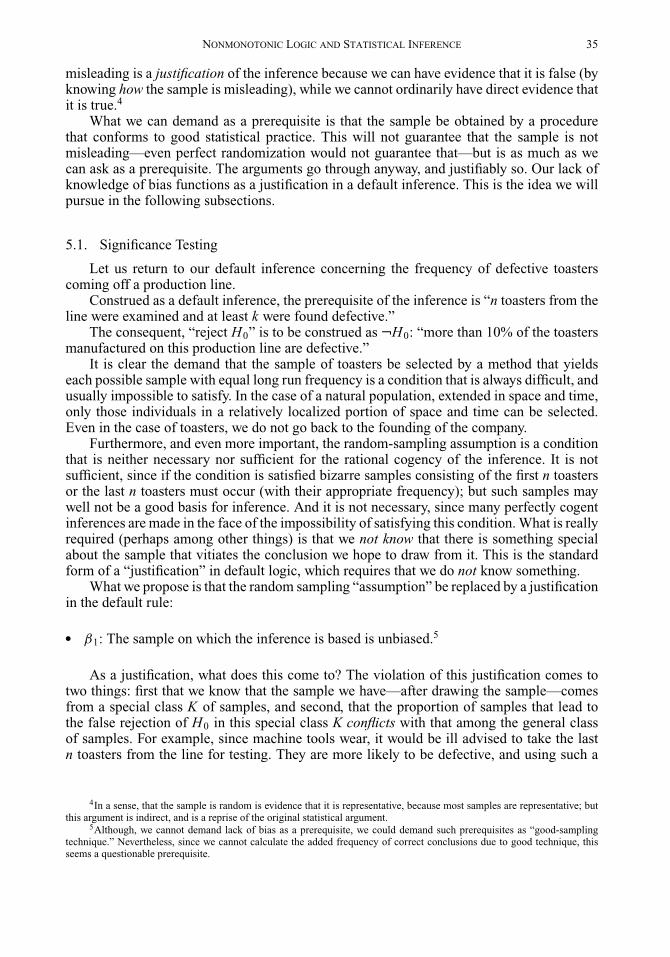
5.1. Significance Testing
Let us return to our default inference concerning the frequency of defective toasterscoming off a production line.
Construed as a default inference, the prerequisite of the inference is “n toasters from theline were examined and at least k were found defective.”
The consequent, “reject H0” is to be construed as ¬H0: “more than 10% of the toastersmanufactured on this production line are defective.”
It is clear the demand that the sample of toasters be selected by a method that yieldseach possible sample with equal long run frequency is a condition that is always difficult, andusually impossible to satisfy. In the case of a natural population, extended in space and time,only those individuals in a relatively localized portion of space and time can be selected.Even in the case of toasters, we do not go back to the founding of the company.
Furthermore, and even more important, the random-sampling assumption is a conditionthat is neither necessary nor sufficient for the rational cogency of the inference. It is notsufficient, since if the condition is satisfied bizarre samples consisting of the first n toastersor the last n toasters must occur (with their appropriate frequency); but such samples maywell not be a good basis for inference. And it is not necessary, since many perfectly cogentinferences are made in the face of the impossibility of satisfying this condition. What is reallyrequired (perhaps among other things) is that we not know that there is something specialabout the sample that vitiates the conclusion we hope to draw from it. This is the standardform of a “justification” in default logic, which requires that we do not know something.
What we propose is that the random sampling “assumption” be replaced by a justificationin the default rule:� β1: The sample on which the inference is based is unbiased.5
As a justification, what does this come to? The violation of this justification comes totwo things: first that we know that the sample we have—after drawing the sample—comesfrom a special class K of samples, and second, that the proportion of samples that lead tothe false rejection of H0 in this special class K conflicts with that among the general classof samples. For example, since machine tools wear, it would be ill advised to take the lastn toasters from the line for testing. They are more likely to be defective, and using such a
4In a sense, that the sample is random is evidence that it is representative, because most samples are representative; butthis argument is indirect, and is a reprise of the original statistical argument.
5Although, we cannot demand lack of bias as a prerequisite, we could demand such prerequisites as “good-samplingtechnique.” Nevertheless, since we cannot calculate the added frequency of correct conclusions due to good technique, thisseems a questionable prerequisite.

36 COMPUTATIONAL INTELLIGENCE
sample would lead to the excessively frequent false rejection of H0, which concerns long runaverage conditions.
If we draw a sample of toaster knobs (the plastic dials controlling the temperature) fromthe top of a crate to make an inference concerning the proportion of cracked knobs, we willalmost surely be wrong: cracked knobs tend to fall to the bottom of the crate.
This is a matter of something we know: we know that samples from the top of the crate areless frequently representative of the proportion of cracked knobs than are stratified samples—samples taken proportionally from several levels of the crate. Of course a sample from thetop could be representative; and a stratified sample could be misleading. But we must gowith the probabilities.
The mere possibility of having gotten a misleading sample should not inhibit our in-ference. In the absence of evidence to the contrary, the inference goes through. When thereis evidence against fairness—and note that this may be statistical evidence, which couldperfectly well be derived from the very sample we have drawn—the inference is blocked.
In short, the sample must not be known to belong to any alternative subclass that wouldserve as a reference class for a conflicting inference.
Of course there are other conditions that must be satisfied for our significance testinginference to be legitimate. We take these to be justifications: items whose denials must notbe “known.”
An obvious justification for the significance test we are discussing is that the sample ofn be the largest sample we have; to have observed n + m toasters from the line, and found atleast k defective would tell us something quite different. So one justification of our statisticalinference is:� β2: The sample of n is the largest appropriate sample we have.
Note that we do not have to know that there is no larger sample. It is perfectly possiblethat some earlier investigator started to look into quality control, began to take a sample, andbecame distracted. If we cannot combine his data with ours, there is surely no reason not touse the data we have for our inference. On the other hand, it would clearly be wrong to usewhat we know to be only part of the data.
A third justification pertains to prior knowledge. If we knew that under similar circum-stances the relative frequency of error for H0 were 0.25, as opposed to the α value of 0.05,that would surely have a bearing on our significance test inference. We might formulate thisas follows:� β3: There is no known set of prior distributions such that conditioning on them with the
data obtained leads to a probability interval conflicting with 1 − α.6
Note that we suppose here that even if our prior knowledge is vague—represented by aset of distributions, rather than a single distribution—we may find conflict with the size ofthe significance test. Thus if H0 were given a high enough prior probability, that probabilitycould undermine the result of the significance test.
Something like this may well be going on in the case of tests of psychic phenomenaand other controversial statistical inferences. Of course one would need to look at individual
6What “conflict” comes to in this instance is an interval that overlaps with, but does not include and is not included in[1 − α, 1].

NONMONOTONIC LOGIC AND STATISTICAL INFERENCE 37
cases, and to evaluate the plausibility of the prior probabilities, to arrive at a useful judgmentabout these matters.
It has long been agreed, even by the founding fathers of statistics, that if one has knowledgeof a prior distribution for a parameter (such as the defect rate in our toaster production line),we should use that knowledge (Fisher 1930; Neyman 1957). This is seldom or never madeexplicit as a premise, but fits in nicely as a justification for a default rule.
5.2. Hypothesis Testing
Let us consider the test of a hypothesis H0, the hypothesis that the relative frequency ofB’s among A’s is 1/3, against the alternative hypothesis H1 that the relative frequency of B’samong A’s is 3/4.
We test H0 against H1 by drawing a sample of five A’s, and observing the number ofB’s. If we observe four or five B’s, we reject H0. Error of the first kind, the chance of a falserejection of H0, is 0.045. Error of the second kind consists of failure to reject H0 when it isfalse. This is the long run frequency with which the hypothesis under test will be mistakenlyaccepted. Since the alternative H1 to H0 is simple, we can calculate this, too; it is 0.367.
Since we are taking as a premise—a prerequisite—that one or the other of these hypothe-ses is true, these are the only errors we can make in this test. Our before test chance of erroris best characterized by the interval [0.045, 0.367].
The default rule for the inference in which we reject H0 looks like this:
Prerequisite: (H0 ∨ H1) ∧ of a sample of five there are four or five B’s.Conclusion: ¬H0.Confidence (1 − θ ): 1 − 0.045 = 0.955.Justifications:
β1: This is the largest relevant sample.β2: This sample is unbiased.β3: There is no prior probability that gives rise, by conditioning, to a conflicting confidence.
Since we make an error in the legitimate application of this rule if and only if H0 is true, itseems plausible to say that the probability of H0 is 0.045. (Of course, classical statisticians willdeny that 0.045 is any kind of any probability; that reflects evidential rather than frequencyprobability.) But clearly if we have good reason to assign a high-prior probability to H0,conditioning may undermine our hypothesis test. If the probability of H0 is [p, q], andp ≥ 0.399, then the lower bound for the probability of H0 conditioned on the observation offour or five B’s in our sample of five A’s is greater than 0.045. In the case of such conflict itseems intuitive to take the probability based on the richer background knowledge as correct,in accord with Rule I for evidential probability.
There may be other justifications that could be mentioned, but we believe they are oftenreducible to these. Note that both size α and power 1 − β of classical tests are long runrelative frequencies. They are grounded semantically in facts about the world.
5.3. Confidence Intervals
This is a default version of confidence interval inference. We take ln(r ) and un(r ) to bethe lower and upper 1 − θ confidence bounds for a binomial sample of size n with the sampleratio r.

38 COMPUTATIONAL INTELLIGENCE
The default rule is:Prerequisite: s is a sample of n A’s of which a fraction r are B’s.Conclusion: The proportion of A’s that are B’s lies between ln(r ) and un(r ).Confidence: The conclusion is categorically asserted with confidence 1 − θ .
Again, the interesting part of the rule is its set of justifications:
β1: s is the largest sample of A’s we have.β2: s is not biased.
Put otherwise, we must not know that the sample is drawn from a class of samples inwhich the frequency of representative samples is less than that among the set of sampleson which the statistical inference is based. Note that we do not have to “know” that s isnot biased at all; it suffices that there is no default inference of sufficient strength withthe conclusion that s is biased.
β3: A is not known to be a member of a set of populations that gives rise, by conditioning,to a probability for the conclusion “The proportion of A’s that are B’s lies between ln(r )and un(r )” that conflicts with the interval [1 − θ , 1] or falls within it.
β4: There is no secular trend of B’s among the A’s.
Note that the denial of this justification could be established by a default inference from thesame data we would use in this inference. It would then block the confidence interval defaultrule.
Again, there may be other justifications that should be considered, but these seem tocover the most important ones. Although they need not be “known”—taken as part of theevidence—they should be subject to rational debate. Of course, to list β as a justificationdoes not preclude the possibility that it is known; if it is known, so much the better. What isprecluded is the use of the default rule when the negation of β is known.
6. COMPETING DEFAULTS
Statistical inference can be modeled as default inference. We can construct normativedefault rules based on these statistical inference principles. For instance, using confidenceinterval calculations we may say (with confidence 0.95) the proportion of birds that fly is inthe interval [0.93, 0.97]. This gives us a reason to adopt the default rule
bird : fly, β1, β2, . . .
fly,
where the β i ’s correspond to the justifications discussed in the previous section. Similarly,we may at the same time obtain another default rule
penguin : ¬fly, β ′1, β
′2, . . .
¬fly.
In general we can think of a default rule as being well justified if its associated confidenceinterval is “high”; for example, if the lower bound of the interval exceeds a certain rulethreshold 1 − θ .
Both of the above rules can be well supported by the underlying statistics, yet in the caseof an object being both a bird and a penguin, the two rules offer conflicting conclusions. Inthis section, we consider the problem of choosing between competing defaults.

NONMONOTONIC LOGIC AND STATISTICAL INFERENCE 39
6.1. Conflicts
Consider the following canonical example.
Example 1. We have a default theory = 〈F, D〉, where
F = {R, S },
D ={
R : T, β1, β2, . . .
T,
S : ¬T, β ′1, β
′2, . . .
¬T
}.
We get two extensions, one containing T and the other containing ¬T . If we take R to mean“bird,” S to mean “penguin,” and T to mean “fly,” then we would like to reject the extensioncontaining T (fly) in favor of the extension containing ¬T (not fly). However, if we take S tomean “animal” instead and keep the interpretations of R and T the same, we would want toreverse our preference. Now the extension containing T (fly) seems more reasonable.
Note that each of the default rules involved in the example above is intuitively appealingwhen viewed by itself against our background knowledge: birds fly; penguins do not fly; andanimals in general do not fly either. Moreover, both instantiations (penguins and animals) aresyntactically indistinguishable. We cannot base our decision to prefer one default rule overthe other by simply looking at their syntactic structures.
There are several approaches to circumventing this conceptual difficulty. The first is torevise the default theory so that the desired result is achieved (Reiter and Criscuolo 1981).We can amend the default rules by adding the exceptions as justifications, for example,
bird : fly, ¬penguin, . . .
fly;
animal : ¬fly, ¬bird, . . .
¬fly.
With this approach we have to constantly revise the default rules to take into account additionalexceptions. We have little guidance in constructing the list of justifications except that theresulting default rule has to produce the “right” answer in the given situation.
Another approach is to establish some priority structure over the set of defaults. Forexample, we can refer to a specificity or inheritance hierarchy to determine which defaultrule should be used in case of a conflict (Touretzky 1984; Horty, Touretzky, and Thomason1987). The penguin rule is more specific than the bird rule, and therefore, when both areapplicable we use the penguin rule and not the bird rule. However, conflicting rules do notalways fit into neat hierarchies (e.g., adults are employed, students are not, how about adultstudents? (Reiter and Criscuolo 1981)). It is not obvious how we can extend the hierarchicalstructure without resorting to explicitly enumerating the priority relations between the defaultrules (Brewka 1989, 1994).
The third approach is to appeal to probabilistic analysis. Defaults are interpreted asrepresenting some infinitesimal probability condition. Adams requires that for A to be a rea-sonable consequence of the set of sentences S, for any ε there must be a positive δ suchthat for every probability function, if the probability of every sentence in S is greater than1 − δ, then the probability of A is at least 1 − ε (Adams 1966, 1975). Pearl’s approachsimilarly involves quantification over possible probability functions (Pearl 1988, 1990).Bacchus et al. (1993) again take the degree of belief appropriate to a statement to be theproportion or limiting proportion of intended first-order models in which the statement istrue.
All of these approaches involve matters that go well beyond what we may reasonablysuppose to be available to us as empirical enquirers. In contrast, our approach to constructing
40 COMPUTATIONAL INTELLIGENCE
default rules is modeled on statistical inference. The confidence parameter α and the rulethreshold 1 − θ reflect established statistical procedures.
We have argued for the distinction between prerequisites and justifications in nonmono-tonic reasoning. In particular, many “assumptions” in statistical inference should be codedas justifications, which are acceptable unless shown false, as opposed to the stronger prereq-uisites, which are acceptable only if they can be proven true. Many logics of conditionals, forexample, along the lines of System P (Kraus, Lehman, and Magidor 1990), do not providefor such a distinction. In addition, there are some limitations that make a logic based onconditionals unsatisfactory for nonmonotonic inference. For a more complete discussion ofthese issues, see Kyburg, Teng, and Wheeler (Forthcoming).
Our principles for constructing default rules and resolving conflicts among them arein the same spirit as the approaches taken in Kyburg (1974) and Pollock (1990). Theseprinciples may not account for all our intuitions regarding conflicting default rules, but forthe large number of rules that are based mainly on our knowledge of or intuitions aboutrelative frequencies, they seem to offer sensible guidance.
6.2. A Fourth Approach
We can methodically resolve some of the conflicts posed by rules such as those discussedin Example 1. The appropriate default rule to be applied can be picked out by reference to thestatistical information supporting the rules. This provides an accountable basis for decidingbetween rules and, therefore, extensions.
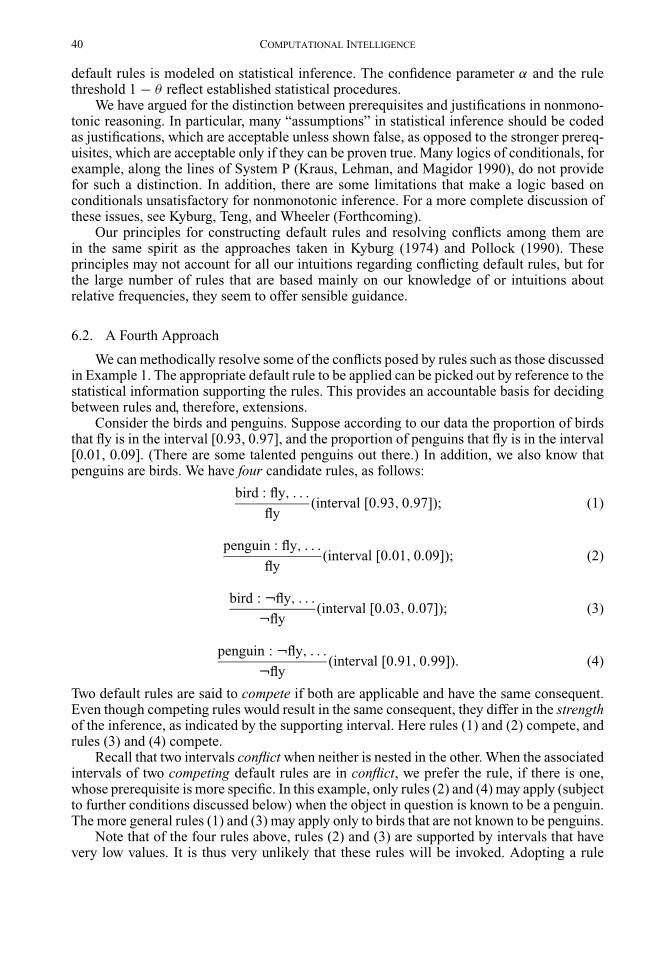
Consider the birds and penguins. Suppose according to our data the proportion of birdsthat fly is in the interval [0.93, 0.97], and the proportion of penguins that fly is in the interval[0.01, 0.09]. (There are some talented penguins out there.) In addition, we also know thatpenguins are birds. We have four candidate rules, as follows:
bird : fly, . . .
fly(interval [0.93, 0.97]); (1)
penguin : fly, . . .
fly(interval [0.01, 0.09]); (2)
bird : ¬fly, . . .
¬fly(interval [0.03, 0.07]); (3)
penguin : ¬fly, . . .
¬fly(interval [0.91, 0.99]). (4)
Two default rules are said to compete if both are applicable and have the same consequent.Even though competing rules would result in the same consequent, they differ in the strengthof the inference, as indicated by the supporting interval. Here rules (1) and (2) compete, andrules (3) and (4) compete.
Recall that two intervals conflict when neither is nested in the other. When the associatedintervals of two competing default rules are in conflict, we prefer the rule, if there is one,whose prerequisite is more specific. In this example, only rules (2) and (4) may apply (subjectto further conditions discussed below) when the object in question is known to be a penguin.The more general rules (1) and (3) may apply only to birds that are not known to be penguins.
Note that of the four rules above, rules (2) and (3) are supported by intervals that havevery low values. It is thus very unlikely that these rules will be invoked. Adopting a rule

NONMONOTONIC LOGIC AND STATISTICAL INFERENCE 41
threshold of, for instance, 0.80 would exclude these rules from being applied in practice.However, rule (2) still competes with rule (1), and is preferred to rule (1), as far as penguinsare concerned. By the same token, rule (4) is preferred to rule (3), but this time rule (4) islikely to be applied, as the associated interval is above the rule threshold. This allows us toconclude that penguins do not fly.
Now consider another case. Suppose we also have information about red birds; theproportion of red birds that fly is in the interval [0.60, 1.00]. Red birds are of course alsobirds, but this time we should not prefer the more specific inference. The information aboutred birds is vague (perhaps because there are few occurrences of red birds in our data). Thereis no conflict between the interval for red birds [0.60, 1.00] and the interval for birds ingeneral [0.93, 0.97]. In this case, even though red birds are more specific, the associatedstatistical information does not warrant the construction of a separate rule for this subclass.We have only rules (1) and (3) above, and they apply to all birds, red or otherwise.
Now let us look at the Nixon diamond. Suppose the proportion of pacifists among quakersis in the interval [0.85, 0.95], and the proportion of pacifists among Republicans is in theinterval [0.20, 0.25]. What can we say about Nixon, who is both a quaker and a Republican?
The four candidate rules are
quaker : pacifist, . . .
pacifist(interval [0.85, 0.95]); (5)
Republican : pacifist,. . .
pacifist(interval [0.20, 0.25]); (6)
quaker : ¬pacifist,. . .
¬pacifist(interval [0.05, 0.15]); (7)
Republican : ¬pacifist,. . .
¬pacifist(interval [0.75, 0.80]). (8)
Rules (5) and (6) compete, and rules (7) and (8) compete. In addition, the intervals ofthe rules in each pair conflict. Unlike penguins and birds, the two reference classes here,quakers and Republicans do not have a subset relationship. When the competing rules areboth applicable, as in the case for Nixon, and the conflict cannot be resolved by appealingto subset relationships between the reference classes, we take the cover of the conflictingintervals. This is equivalent to preferring the following rules when the person in question isboth a quaker and a Republican.
quaker ∧ Republican : pacifist,. . .
pacifist(interval [0.20, 0.95]);
quaker ∧ Republican : ¬pacifist,. . .
¬pacifist(interval [0.05, 0.80]).
The wide intervals reflect the conflicts; we are unlikely to invoke either of these rules as theyare not likely to be above our chosen threshold of acceptance.
6.3. Principles for Resolving Conflicts
We can adjudicate between competing default rules by considering the supporting statis-tical information. A preferred candidate rule is applied only when it is above the given rule
42 COMPUTATIONAL INTELLIGENCE
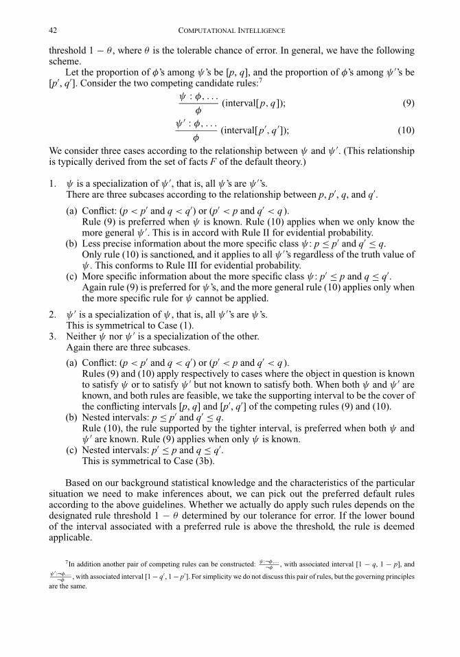
threshold 1 − θ , where θ is the tolerable chance of error. In general, we have the followingscheme.
Let the proportion of φ’s among ψ’s be [p, q], and the proportion of φ’s among ψ ′’s be[p′, q′]. Consider the two competing candidate rules:7
ψ : φ, . . .
φ(interval[p, q]); (9)
ψ ′ : φ, . . .
φ(interval[p′, q ′]); (10)
We consider three cases according to the relationship between ψ and ψ ′. (This relationshipis typically derived from the set of facts F of the default theory.)
1. ψ is a specialization of ψ ′, that is, all ψ’s are ψ ′’s.There are three subcases according to the relationship between p, p′, q, and q′.
(a) Conflict: (p < p′ and q < q′) or (p′ < p and q′ < q ).Rule (9) is preferred when ψ is known. Rule (10) applies when we only know themore general ψ ′. This is in accord with Rule II for evidential probability.
(b) Less precise information about the more specific class ψ : p ≤ p′ and q′ ≤ q.Only rule (10) is sanctioned, and it applies to all ψ ′’s regardless of the truth value ofψ . This conforms to Rule III for evidential probability.
(c) More specific information about the more specific class ψ : p′ ≤ p and q ≤ q′.Again rule (9) is preferred for ψ’s, and the more general rule (10) applies only whenthe more specific rule for ψ cannot be applied.
2. ψ ′ is a specialization of ψ , that is, all ψ ′’s are ψ’s.This is symmetrical to Case (1).
3. Neither ψ nor ψ ′ is a specialization of the other.Again there are three subcases.
(a) Conflict: (p < p′ and q < q′) or (p′ < p and q′ < q ).Rules (9) and (10) apply respectively to cases where the object in question is knownto satisfy ψ or to satisfy ψ ′ but not known to satisfy both. When both ψ and ψ ′ areknown, and both rules are feasible, we take the supporting interval to be the cover ofthe conflicting intervals [p, q] and [p′, q′] of the competing rules (9) and (10).
(b) Nested intervals: p ≤ p′ and q′ ≤ q.Rule (10), the rule supported by the tighter interval, is preferred when both ψ andψ ′ are known. Rule (9) applies when only ψ is known.
(c) Nested intervals: p′ ≤ p and q ≤ q′.This is symmetrical to Case (3b).
Based on our background statistical knowledge and the characteristics of the particularsituation we need to make inferences about, we can pick out the preferred default rulesaccording to the above guidelines. Whether we actually do apply such rules depends on thedesignated rule threshold 1 − θ determined by our tolerance for error. If the lower boundof the interval associated with a preferred rule is above the threshold, the rule is deemedapplicable.
7In addition another pair of competing rules can be constructed: ψ :¬φ,...¬φ
, with associated interval [1 − q, 1 − p], and
ψ ′:¬φ,...¬φ
, with associated interval [1 − q′, 1 − p′]. For simplicity we do not discuss this pair of rules, but the governing principles
are the same.

NONMONOTONIC LOGIC AND STATISTICAL INFERENCE 43
To recapitulate, we remove from the set of competing rules the less specific and vaguerrules. Of the remaining we take the cover of their associated intervals, and apply only thosewhose lower bounds are above the rule threshold. These principles for resolving conflictsbetween competing default rules are analogous to the ones developed for choosing betweenreference classes in an evidential probability setting (Kyburg and Teng 2001).
This statistical approach provides the normative guidance that is lacking in the ad hocapproach to revising default rules. Instead of relying on intuition to tweak the default rulesuntil they give the “right” results, our preferred rules are systematically generated from theunderlying statistics.
7. STATISTICAL DEFAULT THEORIES
The previous section deals with the problem of adjudicating potential conflicts betweencompeting default rules. The rules that are inappropriate in a particular situation are excludedfrom consideration based on a number of principles. Applying a single rule constitutes onestep in the inference process. When we consider the grander picture of default extensions,we need to take into account the effect of cumulative inference. An extension typically isderived from multiple inferences, some of whose applicability is dependent upon previousdefault conclusions. Statistical default rules and statistical default theories take into accountsuch cumulative effects in their formulation.
7.1. Statistical Considerations
An important feature of classical statistical inference is its emphasis on the control oferror (Mayo 1996). A corollary of this emphasis is that we may want to acknowledge explicitlyin our inference forms the upper limit of the frequency with which error may be committed.This represents a difference between our statistical defaults and standard defaults. In thecase of the statistical default rule there is an unavoidable, if controlled, chance of error. Thesignificance test default in Section 5.1 will yield a false rejection of H0 up to a fraction α ofthe time.
We have suggested rejecting the requirement that samples be strictly random, in favor ofthe requirement that we not know that they are biased. But this latter knowledge may be quiteweak; all we require in order for our inference to be blocked is some sort of “good reason,”which may itself come from a statistical default, for thinking our sample biased.
Furthermore, there is the question of the interaction between sentences in a default exten-sion. In Reiter’s formulation a default extension is deductively closed. However, when dealingwith statistical inferences, the bounds on the frequency of error for individual conclusionsdo not carry over unchanged when multiple conclusions are considered together. Acceptinga hypothesis H0 with confidence 0.95 and accepting another hypothesis H1 independentlywith confidence 0.95 do not entail the acceptance of both H0 and H1 simultaneously at aconfidence level of 0.95.
The same consideration goes for the chaining of default inferences. In the standard defaultlogic setting, once a default consequent is asserted it enjoys the same status as the “facts”that were originally given in the knowledge base.8 Such a default consequent can be used tosatisfy a prerequisite condition of an otherwise inapplicable default rule. Thus, the rules canbe chained to obtain further conclusions based on previous default inferences.
8At least until we discover an inconsistency and need to retract some conclusions.
44 COMPUTATIONAL INTELLIGENCE
This makes sense in a qualitative framework, but where defaults are based on statistics,it is clear that the more the number of steps involved, the lower the level of confidence thatcan be attributed to a conclusion thus obtained.
Given these considerations of statistically motivated default inference, a thresholdingmechanism is introduced to coordinate the interactions which give rise to a default extension.The resulting statistical defaults and statistical default theories are discussed in the followingsection.
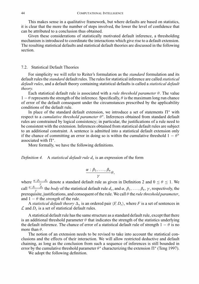
7.2. Statistical Default Theories
For simplicity we will refer to Reiter’s formulation as the standard formulation and itsdefault rules the standard default rules. The rules for statistical inference are called statisticaldefault rules, and a default theory containing statistical defaults is called a statistical defaulttheory.
Each statistical default rule is associated with a rule threshold parameter θ . The value1 − θ represents the strength of the inference. Specifically, θ is the maximum long run chanceof error of the default consequent under the circumstances prescribed by the applicabilityconditions of the default rule.
In place of the standard default extension, we introduce a set of statements �∗ withrespect to a cumulative threshold parameter θ∗. Inferences obtained from standard defaultrules are constrained by logical consistency; in particular, the justifications of a rule need tobe consistent with the extension. Inferences obtained from statistical default rules are subjectto an additional constraint. A sentence is admitted into a statistical default extension onlyif the chance of committing an error in doing so is within the cumulative threshold 1 − θ∗associated with �∗.
More formally, we have the following definitions.
Definition 4. A statistical default rule ds is an expression of the form
α : β1, . . . , βn
γθ,
where α : β1,...,βn
γdenote a standard default rule as given in Definition 2 and 0 ≤ θ ≤ 1. We
call α : β1,...,βn
γthe body of the statistical default rule ds , and α, β1, . . . , βn, γ , respectively, the
prerequisite, justifications, and consequent of the rule. We call θ the rule threshold parameter,and 1 − θ the strength of the rule.
A statistical default theory s is an ordered pair 〈F, Ds〉, where F is a set of sentences inL and Ds is a set of statistical default rules.
A statistical default rule has the same structure as a standard default rule, except that thereis an additional threshold parameter θ that indicates the strength of the statistics underlyingthe default inference. The chance of error of a statistical default rule of strength 1 − θ is nomore than θ .
The notion of an extension needs to be revised to take into account the statistical con-clusions and the effects of their interaction. We will allow restricted deductive and defaultchaining, as long as the conclusion from such a sequence of inferences is still bounded inerror by the cumulative threshold parameter θ∗ characterizing the extension �∗ (Teng 1997).
We adopt the following definition.
NONMONOTONIC LOGIC AND STATISTICAL INFERENCE 45
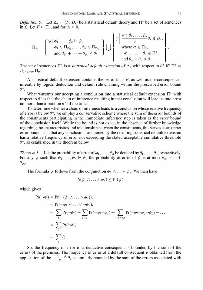
Definition 5. Let s = 〈F, Ds〉 be a statistical default theory and �∗ be a set of sentencesin L. Let F ⊆ �0, and for θ i ≥ 0,
�θi =⎧⎨⎩
ψ | φ1, . . . , φk � ψ,
φ1 ∈ �θφ1, . . . , φk ∈ �θφk
,
and θφ1+ · · · + θφk ≤ θi
⎫⎬⎭ ⋃⎧⎪⎪⎪⎪⎪⎨⎪⎪⎪⎪⎪⎩
γ
∣∣∣∣ α : β1, . . . , βn
γθs ∈ Ds,
where α ∈ �θα,
¬β1, . . . , ¬βn �∈ �∗,and θα + θs ≤ θi
⎫⎪⎪⎪⎪⎪⎬⎪⎪⎪⎪⎪⎭.
The set of sentences �∗ is a statistical default extension of s with respect to θ∗ iff �∗ =∪0≤θi ≤θ∗�θi .
A statistical default extension contains the set of facts F, as well as the consequencesinferable by logical deduction and default rule chaining within the prescribed error boundθ∗.
What warrants our accepting a conclusion into a statistical default extension �∗ withrespect to θ∗ is that the chain of inference resulting in that conclusion will lead us into errorno more than a fraction θ∗ of the time.
To determine whether a chain of inference leads to a conclusion whose relative frequencyof error is below θ∗, we employ a conservative scheme where the sum of the error bounds ofthe constituents participating in the immediate inference step is taken as the error boundof the conclusion itself. While the bound is not exact, in the absence of further knowledgeregarding the characteristics and relationship between the constituents, this serves as an uppererror bound such that any conclusion sanctioned by the resulting statistical default extensionhas a relative frequency of error not exceeding the stated acceptable cumulative thresholdθ∗, as established in the theorem below.
Theorem 1. Let the probability of error of φ1, . . . , φn be denoted by θ1, . . . , θn , respectively.For any ψ such that φ1, . . . , φn � ψ , the probability of error of ψ is at most θφ1
+· · ·+θφn .
The formula ψ follows from the conjunction φ1 ∧ . . . ∧ φn . We then have
Pr(φ1 ∧ . . . ∧ φn) ≤ Pr(ψ),
which gives
Pr(¬ψ) ≤ Pr(¬(φ1 ∧ . . . ∧ φn)),
= Pr(¬φ1 ∨ . . . ∨ ¬φn),
=∑
i
Pr(¬φi ) −∑i< j
Pr(¬φi¬φ j ) +∑
i< j<k
Pr(¬φi¬φ j¬φk) − . . .
≤∑
i
Pr(¬φi )
=∑
i
θi .
So, the frequency of error of a deductive consequent is bounded by the sum of theerrors of the premises. The frequency of error of a default consequent γ obtained from the
application of the α : β1,...,βn
γθs is similarly bounded by the sum of the errors associated with
46 COMPUTATIONAL INTELLIGENCE
the prerequisite (θα) and with the rule itself (θ s ). In addition, for the rule to be applicable,the negation of each of the justifications must be excluded from the extension �∗.
A standard default rule can be represented as a statistical default rule with strength1 (θ = 0). In other words, a standard default rule
α : β1, . . . , βn
γ
can be rewritten as
α : β1, . . . , βn
γ0
in the statistical default framework.Note that this does not mean that standard default rules have a zero chance of error, and are
therefore always correct. A θ value of 0 in this case merely denotes that the rules in questionare qualitative and are thus subjected only to the qualitative constraints, namely, logicalconsistency. The formulation of a statistical default extension is such that the application ofa qualitative default rule (with θ = 0) does not add to the cumulative error of the formulasderived via this default rule.
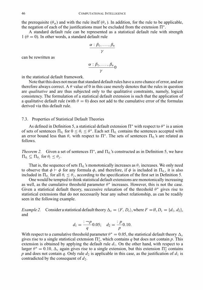
7.3. Properties of Statistical Default Theories
As defined in Definition 5, a statistical default extension �∗ with respect to θ∗ is a unionof sets of sentences �θi for 0 ≤ θi ≤ θ∗. Each set �θi contains the sentences accepted withan error bound less than θ i with respect to �∗. The sets of sentences �θi ’s are related asfollows.
Theorem 2. Given a set of sentences �∗, and �θi ’s constructed as in Definition 5, we have�θi ⊆ �θ j for θi ≤ θ j .
That is, the sequence of sets �θi ’s monotonically increases as θ i increases. We only needto observe that φ � φ for any formula φ, and therefore, if φ is included in �θi , it is alsoincluded in �θ j for all θi ≤ θ j , according to the specification of the first set in Definition 5.
One would be tempted to think statistical default extensions are monotonically increasingas well, as the cumulative threshold parameter θ∗ increases. However, this is not the case.Given a statistical default theory, successive relaxation of the threshold θ∗ gives rise tostatistical extensions that do not necessarily bear any subset relationship, as can be readilyseen in the following example.
Example 2. Consider a statistical default theorys = 〈F, Ds〉, where F =∅, Ds = {d1, d2},and
d1 = : ¬p
q0.05; d2 = : p
p0.10.
With respect to a cumulative threshold parameter θ∗ = 0.05, the statistical default theory sgives rise to a single statistical extension �∗
1, which contains q but does not contain p. Thisextension is obtained by applying the default rule d1. On the other hand, with respect to alarger θ∗ = 0.10, s again gives rise to a single extension, but this extension �∗
2 containsp and does not contain q. Only rule d2 is applicable in this case, as the justification of d1 iscontradicted by the consequent of d2.
NONMONOTONIC LOGIC AND STATISTICAL INFERENCE 47
The two sets of sentences �∗1 and �∗
2 are overlapping (e.g., they both contain the tau-tologies), but each contains elements that are not in the other set.
Thus, as the cumulative threshold parameter θ∗ increases, the extensions obtained from astatistical default theory do not form a monotonic sequence. Even the existence of extensionswith respect to one θ∗ does not provide any guarantee for the existence of extensions withrespect to other values of the threshold. This is shown in the following example.
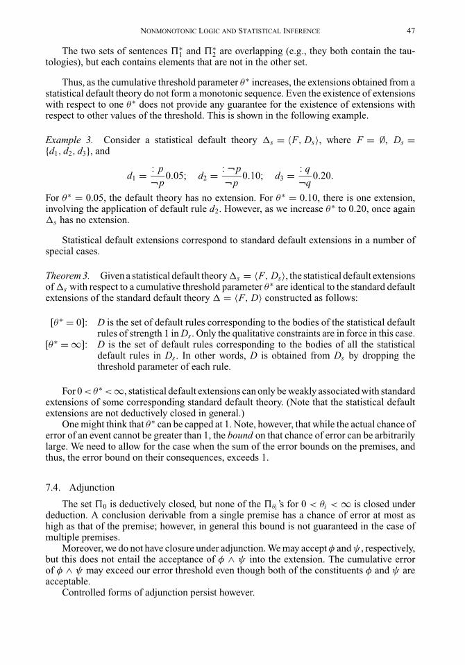
Example 3. Consider a statistical default theory s = 〈F, Ds〉, where F = ∅, Ds ={d1, d2, d3}, and
d1 = : p
¬p0.05; d2 = : ¬p
¬p0.10; d3 = : q
¬q0.20.
For θ∗ = 0.05, the default theory has no extension. For θ∗ = 0.10, there is one extension,involving the application of default rule d2. However, as we increase θ∗ to 0.20, once agains has no extension.
Statistical default extensions correspond to standard default extensions in a number ofspecial cases.
Theorem 3. Given a statistical default theorys = 〈F, Ds〉, the statistical default extensionsof s with respect to a cumulative threshold parameter θ∗ are identical to the standard defaultextensions of the standard default theory = 〈F, D〉 constructed as follows:
[θ∗ = 0]: D is the set of default rules corresponding to the bodies of the statistical defaultrules of strength 1 in Ds . Only the qualitative constraints are in force in this case.
[θ∗ = ∞]: D is the set of default rules corresponding to the bodies of all the statisticaldefault rules in Ds . In other words, D is obtained from Ds by dropping thethreshold parameter of each rule.
For 0 <θ∗ <∞, statistical default extensions can only be weakly associated with standardextensions of some corresponding standard default theory. (Note that the statistical defaultextensions are not deductively closed in general.)
One might think that θ∗ can be capped at 1. Note, however, that while the actual chance oferror of an event cannot be greater than 1, the bound on that chance of error can be arbitrarilylarge. We need to allow for the case when the sum of the error bounds on the premises, andthus, the error bound on their consequences, exceeds 1.
7.4. Adjunction
The set �0 is deductively closed, but none of the �θi ’s for 0 < θi < ∞ is closed underdeduction. A conclusion derivable from a single premise has a chance of error at most ashigh as that of the premise; however, in general this bound is not guaranteed in the case ofmultiple premises.
Moreover, we do not have closure under adjunction. We may accept φ and ψ , respectively,but this does not entail the acceptance of φ ∧ ψ into the extension. The cumulative errorof φ ∧ ψ may exceed our error threshold even though both of the constituents φ and ψ areacceptable.
Controlled forms of adjunction persist however.
48 COMPUTATIONAL INTELLIGENCE
If φ ∈ �θφ, φ � ψ1, and φ � ψ2, then ψ1 ∧ ψ2 ∈ �θφ
.If φ ∈ �θφ
, ψ ∈ �θψ, and θφ + θψ ≤ θ∗, then φ ∧ ψ ∈ �θφ+θψ
⊆ �∗.
In the first case, ψ1 ∧ ψ2 is accepted at the error threshold θφ if both conjuncts ψ1 andψ2 can be derived from the same premise φ that is itself acceptable at the error threshold θφ .
In the second case, we accept φ ∧ ψ provided that the sum of errors collectively inducedby the conjuncts φ and ψ is below the cumulative threshold parameter θ∗ of the statisticalextension �∗. The frequency of error of φ ∧ ψ is bounded by θφ + θψ .
Restricted adjunction gives rise to a logic that can be paraconsistent, as shown in thefollowing example.
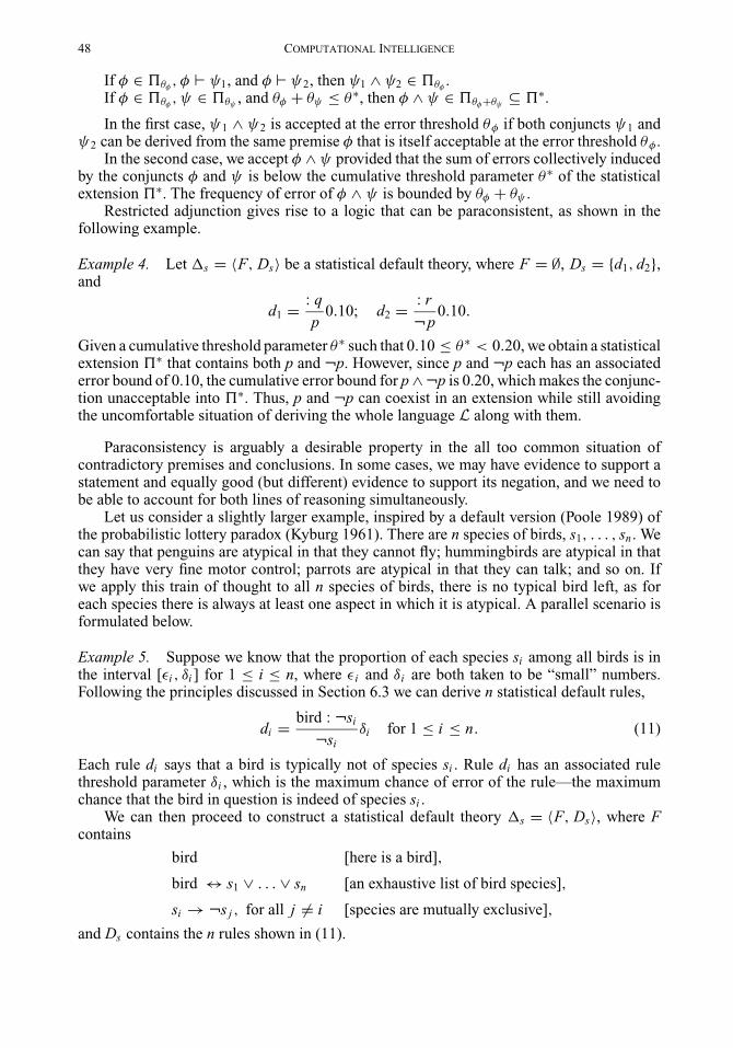
Example 4. Let s = 〈F, Ds〉 be a statistical default theory, where F = ∅, Ds = {d1, d2},and
d1 = : q
p0.10; d2 = : r
¬p0.10.
Given a cumulative threshold parameter θ∗ such that 0.10 ≤ θ∗ < 0.20, we obtain a statisticalextension �∗ that contains both p and ¬p. However, since p and ¬p each has an associatederror bound of 0.10, the cumulative error bound for p ∧ ¬p is 0.20, which makes the conjunc-tion unacceptable into �∗. Thus, p and ¬p can coexist in an extension while still avoidingthe uncomfortable situation of deriving the whole language L along with them.
Paraconsistency is arguably a desirable property in the all too common situation ofcontradictory premises and conclusions. In some cases, we may have evidence to support astatement and equally good (but different) evidence to support its negation, and we need tobe able to account for both lines of reasoning simultaneously.
Let us consider a slightly larger example, inspired by a default version (Poole 1989) ofthe probabilistic lottery paradox (Kyburg 1961). There are n species of birds, s1, . . . , sn . Wecan say that penguins are atypical in that they cannot fly; hummingbirds are atypical in thatthey have very fine motor control; parrots are atypical in that they can talk; and so on. Ifwe apply this train of thought to all n species of birds, there is no typical bird left, as foreach species there is always at least one aspect in which it is atypical. A parallel scenario isformulated below.
Example 5. Suppose we know that the proportion of each species si among all birds is inthe interval [εi , δi ] for 1 ≤ i ≤ n, where εi and δi are both taken to be “small” numbers.Following the principles discussed in Section 6.3 we can derive n statistical default rules,
di = bird : ¬si
¬siδi for 1 ≤ i ≤ n. (11)
Each rule di says that a bird is typically not of species si . Rule di has an associated rulethreshold parameter δi , which is the maximum chance of error of the rule—the maximumchance that the bird in question is indeed of species si .
We can then proceed to construct a statistical default theory s = 〈F, Ds〉, where Fcontains
bird [here is a bird],
bird ↔ s1 ∨ . . . ∨ sn [an exhaustive list of bird species],
si → ¬s j , for all j �= i [species are mutually exclusive],
and Ds contains the n rules shown in (11).
NONMONOTONIC LOGIC AND STATISTICAL INFERENCE 49
In the standard formulation of default logic, we would get n extensions, each containingone si and the negations of all the other s j ’s. In other words, for each extension, we wouldconclude that the bird we have is of a particular species. This seems to be an over commitment,given the statistical information that only between εi and δi of birds are of species si .
In the statistical default logic setting, we can have less extreme conclusions. With respectto a cumulative threshold parameter θ∗, where
max(δ1, . . . , δn) ≤ θ∗ < mini
(∑j �=i
δ j
),
all n statistical default rules can be applied to conclude respectively ¬s1, . . . , ¬sn , but wedo not necessarily include in the same statistical extension �∗ any of their deductive conse-quences. Thus, in the extension we can have
s1 ∨ . . . ∨ sn, ¬s1, . . . , ¬sn,
without getting a contradiction. A conjunction of the form ¬si ∧ . . . ∧ ¬s j is included in �∗if and only if δi + · · · + δ j ≤ θ∗.
In the case where θ∗ >∑
j �=i δ j for some i, we would derive ¬s j for all j �= i. These
sentences together with s1 ∨ . . . ∨ sn would give us si , blocking the application of di . Thus,we would have an extension containing si and, for all j �= i, ¬s j .
In the extreme case where θ∗ ≥ maxi (∑
j �=i δ j ), we would get n extensions each con-
taining one positive atom si . The extensions obtained in this case are identical to the onesobtained in the standard default logic setting.
8. CONCLUSION
Much of classical statistical inference can usefully be formulated as default inference,taking advantage of the distinction between prerequisites—statements that must be taken aspremises of the inference—and justifications—statements that must not be known, that is, inwhose presence the inference must fail. For example, in classical confidence inference to themean of a normal distribution, the value of the observation must be known, for otherwise wehave no basis for the inference. But at the same time, we must not know that the item sampledwas obtained by a procedure that is biased toward large values; we must not have reason tobelieve that the sampled item was part of a larger sample about which we have knowledge;and there must be no way of invoking a known prior probability distribution, conditioningon which would give us a conflicting probability.
It is common to have a collection of possible defaults whose conclusions conflict: stu-dents, by default, are not employed; adults, by default, are employed; so what are we to sayabout adult students? Tweety is a penguin and a bird; birds, by default, fly; penguins, by de-fault, do not fly. Many of these conflicting default inferences can be derived from statisticalknowledge. Choosing among these rules, when possible, can be based on the same principlesthat can be invoked in choosing among reference classes in statistical inference (Kyburg andTeng 2001).
Standard defaults rules are qualitative: if the default can be applied, the conclusion maybe included in an extension. Statistical defaults admit the quantitative possibility of error: ifa hypothesis is rejected at the 0.05 level, there is the explicit maximum chance of 0.05 thatthis rejection is in error, and that the hypothesis is nevertheless true. Statistical defaults are
50 COMPUTATIONAL INTELLIGENCE
therefore different from standard defaults in that they include a parameter θ that representsthe maximum chance of error of that inference.
A consequence of this difference is that while a standard default extension is an ordinarydeductively closed logical theory, extensions for statistical default theories are more compli-cated. For one thing, they are not closed under adjunction: if conclusion A may be in error nomore frequently than θ and conclusion B may be in error no more frequently than θ , that doesnot at all mean that the conclusion A ∧ B is similarly constrained to be in error no more oftenthan θ . For similar reasons, we cannot expect the extensions of statistical default theories tobe deductively closed.
However, we can make sense of the extensions of statistical default theories. We investi-gated some properties of statistical default theories and their connection to standard defaulttheories. Here Reiter’s default logic is used as a concrete platform for the discussion, but ourapproach is applicable to other nonmonotonic formalisms as well. The inferential relationsamong statistical default extensions may be reflected in a weak modal logic, the logic ofthresholding (Kyburg and Teng 2002). We claim that these statistical extensions are plausiblecandidates for realistic bodies of knowledge, and may be of use in AI.
REFERENCES
ADAMS, E. 1966. Probability and the logic of conditionals. In Aspects of Inductive Logic. Edited by J. Hintikka
and P. Suppes. Amsterdam, North Holland, pp. 265–316.
ADAMS, E. W. 1975. The Logic of Conditionals. Dordrecht, Reidel.
BACCHUS, F., A. J. GROVE, J. Y. HALPERN, and D. KOLLER. 1993. Statistical foundations for default reasoning.
In Proceedings of the Thirteenth International Joint Conference on Artificial Intelligence, pp. 563–569.
BAIRD, D. 1992. Inductive Logic: Probability and Statistics. Prentice-Hall, Englewood Cliffs, NJ.
BREWKA, G. 1989. Preferred subtheories—An extended logical framework for default reasoning. In Proceedings
of the Eleventh International Joint Conference on Artificial Intelligence, pp. 1043–1048.
BREWKA, G. 1991. Cumulative default logic: In defense of nonmonotonic inference rules. Artificial Intelligence,
50:183–205.
BREWKA, G. 1994. Reasoning about priorities in default logic. In Proceedings of the Twelfth National Conference
on Artificial Intelligence, pp. 940–945.
CHOW, S. L. 1996. Statistical Significance. Sage, London.
CLOPPER, C. J., and E. S. PEARSON. 1934. The use of confidence or fiducial limits illustrated in the case of the
binomial. Biometrika, 26:404–413.
CRAMER, H. 1951. Mathematical Methods of Statistics. Princeton University Press, Princeton, NJ.
DELGRANDE, J. P., T. SCHAUB, and W. K. JACKSON. 1994. Alternative approaches to default logic. Artificial
Intelligence, 70:167–237.
FISHER, R. A. 1930. Inverse probability. Proceedings of the Cambridge Philosophical Society, 26:528–535.
FISHER, R. A. 1971. The Design of Experiments. Hafner, New York.
GELFOND, M., V. LIFSCHITZ, H. PRZYMUSINSKA, and M. TRUSZCZYNSKI. 1991. Disjunctive defaults. In Proceed-
ings of the Second International Conference on Principles of Knowledge Representation and Reasoning,
pp. 230–238.
HORTY, J. F., D. S. TOURETZKY, and R. H. THOMASON. 1987. A clash of intuitions: The current state of nonmono-
tonic multiple inheritance systems. In Proceedings of the Tenth International Joint Conference on Artificial
Intelligence, pp. 476–482.
KRAUS, S., D. LEHMAN, and M. MAGIDOR. 1990. Nonmonotonic reasoning, preferential models and cumulative
logics. Artificial Intelligence, 44:167–207.
NONMONOTONIC LOGIC AND STATISTICAL INFERENCE 51
KYBURG, H. E., JR. 1961. Probability and the Logic of Rational Belief. Wesleyan University Press, Middletown,
CT.
KYBURG, H. E., JR. 1974. The Logical Foundations of Statistical Inference. Reidel, Dordrecht.
KYBURG, H. E., JR., and C. M. TENG. 1999. Statistical inference as default reasoning. International Journal of
Pattern Recognition and Artificial Intelligence, 13:267–283.
KYBURG, H. E., JR., and C. M. TENG. 2001. Uncertain Inference. Cambridge University Press, New York.
KYBURG, H. E., JR., and C. M. TENG. 2002. The logic of risky knowledge. In Electronic Notes in Theoretical
Computer Science, Volume 67. Elsevier Science.
KYBURG, H. E., JR., C. M. TENG, and G. WHEELER. Forthcoming. Conditionals and consequences. Journal of
Applied Logic.
LEHMANN, E. L. 1959. Testing Statistical Hypotheses. John Wiley and Sons, New York.
LUKASZEWICZ, W. 1988. Considerations on default logic: An alternative approach. Computational Intelligence,
4(1):1–16.
MAYO, D. 1996. Error and the Growth of Experimental Knowledge. University of Chicago Press, Chicago.
MCCARTHY, J. 1986. Applications of circumscription to formalizing common sense knowledge. Artificial Intel-
ligence, 28:89–116.
MIKITIUK, A., and M. TRUSZCZYNSKI. 1995. Constrained and rational default logics. In Proceedings of the
Fourteenth International Joint Conference on Artificial Intelligence, pp. 1509–1517.
MOORE, D. S. 1979. Statistics: Concepts and Controversies. W. H. Freeman, San Francisco.
NEYMAN, J. 1957. ‘Inductive behavior’ as a basic concept of philosophy of science. Review of the International
Statistical Institute, 25:5–22.
PEARL, J. 1988. Probabilistic Reasoning in Intelligent Systems. Morgan Kaufmann, San Francisco.
PEARL, J. 1990. System Z: A natural ordering of defaults with tractable applications to default reasoning. InTheoretical Aspects of Reasoning about Knowledge, pp. 121–135.
POLLOCK, J. 1990. Nomic Probability and the Foundations of Induction. Oxford University Press, Oxford.
POOLE, D. 1989. What the lottery paradox tells us about default reasoning. In Proceedings of the First International
Conference on Principles of Knowledge Representation and Reasoning, pp. 333–340.
REITER, R. 1980. A logic for default reasoning. Artificial Intelligence, 13:81–132.
REITER, R., and G. CRISCUOLO. 1981. On interacting defaults. In Proceedings of the Seventh International Joint
Conference on Artificial Intelligence, pp. 270–276.
TENG, C. M. 1997. Sequential thresholds: Context sensitive default extensions. In Proceedings of the Thirteen
Conference of Uncertainty in Artificial Intelligence, pp. 437–444.
TOURETZKY, D. S. 1984. Implicit ordering of defaults in inheritance systems. In Proceedings of the Fifth National
Conference on Artificial Intelligence, pp. 322–325.
Related Documents