Nonlinear structure formation in nonlocal gravity

IPPP/14/ 70 DCPT/14/ 140

Nonlinear structure formation in Nonlocal Gravity

Alexandre Barreira,1, 2, ∗ Baojiu Li,1 Wojciech A. Hellwing,1, 3 Carlton M. Baugh,1 and Silvia Pascoli21Institute for Computational Cosmology, Department of Physics, Durham University, Durham DH1 3LE, U.K.

2Institute for Particle Physics Phenomenology, Department of Physics, Durham University, Durham DH1 3LE, U.K.3Interdisciplinary Centre for Mathematical and Computational Modeling (ICM),

University of Warsaw, ul. Pawinskiego 5a, Warsaw, Poland

We study the nonlinear growth of structure in nonlocal gravity models with the aid of N-body simulation andthe spherical collapse and halo models. We focus on a model in which the inverse-squared of the d’Alembertianoperator acts on the Ricci scalar in the action. For fixed cosmological parameters, this model differs fromΛCDM by having a lower late-time expansion rate and an enhanced and time-dependent gravitational strength(∼ 6% larger today). Compared to ΛCDM today, in the nonlocal model, massive haloes are slightly moreabundant (by ∼ 10% at M ∼ 1014M/h) and concentrated (≈ 8% enhancement over a range of mass scales),but their linear bias remains almost unchanged. We find that the Sheth-Tormen formalism describes the massfunction and halo bias very well, with little need for recalibration of free parameters. The fitting of the haloconcentrations is however essential to ensure the good performance of the halo model on small scales. Fork & 1h/Mpc, the amplitude of the nonlinear matter and velocity divergence power spectra exhibits a modestenhancement of ∼ 12% to 15%, compared to ΛCDM today. This suggests that this model might only bedistinguishable from ΛCDM by future observational missions. We point out that the absence of a screeningmechanism may lead to tensions with Solar System tests due to local time variations of the gravitational strength,although this is subject to assumptions about the local time evolution of background averaged quantities.

I. INTRODUCTION

It has been almost a century since Einstein proposed his the-ory of General Relativity (GR) which is still considered oneof the main pillars of modern physics. The outstanding suc-cess of GR comes mostly from its ability to pass a number ofstringent tests of gravity performed in the Solar System [1].When applied on cosmological scales, however, GR seems tolose some of its appeal as it requires the presence of some un-known form of dark energy in order to explain the observedaccelerated expansion of the Universe. The simplest candi-date for dark energy is a cosmological constant, Λ, but thevalue of Λ required to explain the observations lacks theoreti-cal support. This has provided motivation for the proposal ofalternative gravity models which attempt to reproduce cosmicacceleration without postulating the existence of dark energy.Furthermore, the fact that the laws of gravity have never beentested directly on scales larger than the Solar System justi-fies the exploration of such modifications to GR on cosmo-logical scales. By understanding better the various types ofobservational signatures that different modified gravity mod-els can leave on cosmological observables, one can improvethe chance of identifying any departures from GR, or alterna-tively, extend the model’s observational success into a wholenew regime. Currently, the study of modified gravity modelsis one of the most active areas of research in both theoreticaland observational cosmology [2–5].

Here, we focus on a class of model that has attracted muchattention recently, which is known as nonlocal gravity [6]. Inthese models, the modifications to gravity arise via the addi-tion of nonlocal terms (i.e. which depend on more than onepoint in spacetime) to the Einstein field equations. These

∗ Electronic address: [email protected]

terms typically involve the inverse of the d’Alembertian op-erator, −1, acting on curvature tensors. To ensure causality,such terms must be defined with the aid of retarded Greenfunctions (or propagators). However, it is well known thatsuch retarded operators cannot be derived from standard ac-tion variational principles (see e.g. Sec. 2 of Ref. [6] for a dis-cussion). One way around this is to specify the model in termsof its equations of motion and not in terms of its action. Onemay still consider a nonlocal action to derive a set of causalequations of motion, so long as in the end one replaces, byhand, all of the resulting operators by their retarded versions.Both of these approaches, however, imply that nonlocal mod-els of gravity must be taken as purely phenomenological andshould not be interpreted as fundamental theories. In gen-eral, one assumes that there is an unknown fundamental (lo-cal) quantum field theory of gravity, and the nonlocal modelrepresents only an effective way of capturing the physics ofthe fundamental theory in some appropriate limit.

It was in the above spirit that Ref. [7] proposed a popularnonlocal model of gravity capable of explaining cosmic ac-celeration. In this model, which has been extensively studied(see e.g. Refs. [6, 8–17] and references therein), one addsthe term Rf

(−1R

)to the Einstein-Hilbert action, where R

is the Ricci scalar and f is a free function. As described inRef. [6], the function f can be constructed in such a way thatit takes on different values on the cosmological backgroundand inside gravitationally bound systems. In particular, at thebackground level, f can be tuned to reproduce ΛCDM-likeexpansion histories, but inside regions like the Solar System,one can assume that f vanishes, thus recovering GR com-pletely. This model, however, seems to run into tension withdata sensitive to the growth rate of structure on large scales[16, 17].

More recently, nonlocal terms have also been used to con-struct theories of massive gravity. An example of this is ob-tained by adding directly to the Einstein field equations a term

arX

iv:1

408.

1084

v1 [

astr

o-ph

.CO

] 5

Aug

201

4

2

likem2(gµν−1R

)T[18–21], wherem is a mass scale and T

means the extraction of the transverse part (see also Refs. [22–25] for models in which −1 acts on the Einstein and Riccitensors). This model has no ΛCDM limit for the backgroundevolution, but it can still match the current background expan-sion and growth rate of structure data with a similar goodness-of-fit [21]. Furthermore, Ref. [20] has investigated spheri-cally symmetric static solutions in this model, concluding thatit does not suffer from instabilities that usually plague the-ories of massive gravity. A similar model was proposed byRef. [26], which is characterized by a term ∝ m2R−2Rin the action (see Eq. (1)). Reference [27] showed that thismodel can reproduce current type Ia Supernovae (SNIa) data,although it also has no ΛCDM limit for the background ex-pansion. The time evolution of linear matter density fluctua-tions in this model also differs from that in ΛCDM, but thework of Ref. [27] suggests that the differences between thesetwo models are small enough to be only potentially distin-guishable by future observational missions.

Here, we extend the previous work done for the model ofRefs. [26, 27] by examining its predictions in the nonlinearregime of structure formation. We achieve this by running aset of N-body simulations, which we use to analyse the modelpredictions for the nonlinear matter and velocity divergencepower spectra, and also halo properties such as their abun-dance, bias and concentration. To the best of our knowledgethis is the first time N-body simulations have been used tostudy the nonlinear regime of structure formation in nonlocalgravity cosmologies. N-body simulations are however com-putationally expensive to run. To overcome this, it is com-mon to try to devise semi-analytical formulae that, motivatedby simple physical assumptions, aim to reproduce the resultsfrom the simulations with the calibration of free parameterskept to a minimum. A popular example is given by the Sheth-Tormen halo mass function [28–30] and its use in the halomodel approach for the nonlinear matter power spectrum [31].The performance of the halo model is well understood withinΛCDM, but less so in alternative gravity scenarios. In par-ticular, the free parameters in these formulae might need sub-stantial recalibration in models that differ significantly fromΛCDM (see e.g. Ref. [32]). One of our goals is to assess theperformance of these analytical formulae in nonlocal gravitymodels.

This paper is organized as follows. In Sec. II we present themodel and layout the equations relevant for the backgroundevolution. We also derive the equations of motion for spher-ically symmetric configurations under the quasi-static andweak-field approximations. In Sec. III we present the formu-lae relevant for the calculation of the nonlinear matter powerspectrum in the halo model formalism. In particular, we de-scribe the Sheth-Tormen expressions for the halo mass func-tion and bias, and define the Navarro-Frenk-White (NFW)halo concentration parameter. We also present the equationsrelevant for the linear evolution and spherical collapse of mat-ter overdensities. Our results are presented in Sec. IV, wherewe discuss the results from the N-body simulations and com-pare them with the predictions from the analytical formulae.We also comment on the role that Solar System tests of gravity

could play in setting the observational viability of this model.We summarize our findings in Sec. V.

In this paper, we work with the metric signature(+,−,−,−) and use units in which the speed of light c = 1.Latin indices run over 1, 2, 3 and Greek indices run over0, 1, 2, 3. We use κ = 8πG = 1/M2

Pl interchangeably, whereMPl is the reduced Planck mass and G is Newton’s constant.

II. THE R−2R NONLOCAL GRAVITY MODEL

A. Action and field equations

We consider the nonlocal gravity model of Refs. [26, 27],whose action is given by

A =1

2κ

∫dx4√−g

[R− m2

6R−2R− Lm

], (1)

where g is the determinant of the metric gµν , Lm is the La-grangian density of the matter fluid, R is the Ricci scalar and = ∇µ∇µ is the d’Alembertian operator. To facilitate thederivation of the field equations, and to solve them afterwards,it is convenient to introduce two auxiliary scalar fields definedas

U = −−1R, (2)S = −−1U = −2R. (3)

The solutions to Eqs. (2) and (3) can be obtained by evaluatingthe integrals

U ≡ −−1R (4)

= Uhom(x)−∫

d4y√−g(y)G(x, y)R(y),

S ≡ −−1U (5)

= Shom(x)−∫

d4y√−g(y)G(x, y)U(y),

where Uhom and Shom are any solutions of the homogeneousequations U = 0 and S = 0, respectively, and G(x, y)is any Green function of . The choice of the homogeneoussolutions and of the Green function specify the meaning of theoperator−1. To ensure causality, one should use the retardedversion of the Green function, i.e., the solutions of U (or S)should only be affected by the values ofR (or U ) that lie in itspast light-cone. The homogeneous solutions can be set to anyvalue, which is typically zero, without any loss of generality.In principle, the model predictions can be obtained by solvingEqs. (4) and (5). However, it is convenient to use the fields Uand S to cast the nonlocal action of Eq. (1) in the form of alocal scalar-tensor theory [10, 33, 34] as

A=1

2κ

∫dx4√−g

[R− m2

6RS − ξ1 (U +R)

−ξ2 (S + U)− Lm] , (6)

3

where ξ1 and ξ2 are Lagrange multipliers. The field equationscan then be written as

Gµν −m2

6Kµν = κTµν , (7)

U = −R, (8)S = −U, (9)

with

Kµν ≡ 2SGµν − 2∇µ∇νS − 2∇(µS∇ν)U

+

(2S +∇αS∇αU −

U2

2

)gµν , (10)

and where Tµν = (2/√−g) δ (Lm

√−g) /δgµν is the energy-

momentum tensor of the matter fluid. The use of the scalarfields U and S therefore allows one to obtain the solutions bysolving a set of coupled differential equations, instead of themore intricate integral equations associated with the inversionof a differential operator. These two formulations are, how-ever, not equivalent as explained with detail in many recentpapers (see e.g. Refs.[9, 18, 19, 23, 34–36]): Eqs. (7), (8) and(9) admit solutions that are not solutions of the original nonlo-cal problem. For instance, if U∗ is a solution of Eq. (8), thenU∗+Uhom is also a solution for any Uhom, sinceUhom = 0(the same applies for the field S and Eq. (9)). If one wishesthe differential equations (7), (8) and (9) to describe the non-local model, then one must solve them with the one and onlychoice of initial conditions that is compatible with the choiceof homogeneous solutions in Eqs. (4) and (5). All other ini-tial conditions lead to spurious solutions and should not beconsidered.

B. Background equations

Throughout, we always work with the perturbedFriedmann-Roberston-Walker (FRW) line element in theNewtonian gauge,

ds2 = (1 + 2Ψ) dt2 − a(t)2 (1− 2Φ) γijdxidxj , (11)

where a = 1/(1 + z) is the cosmic scale factor (z is the red-shift) and the gravitational potentials Φ, Ψ are assumed to befunctions of time and space. γij is the spatial sector of themetric, which is taken here to be flat.

At the level of the cosmological background (Φ = Ψ = 0),the two Friedmann equations can be written as

3H2 = κρm + κρde (12)−2H − 3H2 = κpm + κpde, (13)

where we have encapsulated the effects of the nonlocal terminto an effective background "dark energy" density, ρde, andpressure pde, which are given, respectively, by

κρde =m2

6

[6SH2 + 6H ˙S − ˙U ˙S − U2

2

], (14)

κpde = −m2

6

[2S(

2H + 3H2)

+ ¨S (15)

+4H ˙S + ˙U ˙S − U2

2

].

Additionally, Eqs. (8) and (9) yield

¨U + 3H ˙U = 6(H + 2H2

), (16)

¨S + 3H ˙S = −U . (17)(18)

In the above equations, a dot denotes a partial derivative w.r.t.physical time, t, an overbar indicates that we are consideringonly the background average and H = a/a is the Hubbleexpansion rate.

The background evolution in the R−2R model has to beobtained numerically. The differential equations are evolvedstarting from deep into the radiation dominated era (z = 106)with initial conditions for the auxiliary fields U = ˙U = S =˙S = 0. Note that, in the radiation era, the Ricci scalar van-

ishes (R = 6H + 12H2 = 0). Hence, from Eqs. (4) and (5)one sees that these initial conditions are indeed compatiblewith the choice Uhom = Shom = 0. The value of the pa-rameter m is determined by a trial-and-error scheme to yieldthe value of ρde0 that makes the Universe spatially flat, i.e.,ρr0 + ρm0 + ρde0 = ρc0 ≡ 3H2

0/κ, where the subscripts r,m refer to radiation and matter, respectively, the subscript 0

denotes present-day values, and H0 = 100hkm/s/Mpc is thepresent-day Hubble rate.

C. Spherically symmetric nonlinear equations

By assuming that the potentials Φ and Ψ are sphericallysymmetric, one can write the (0, 0) and (r, r) components ofEq. (7), and Eqs. (8) and (9), respectively, as

2

r2

(r2Φ,r

),r −

m2

6

[6SH2 +

4S

r2

(r2Φ,r

),r −

2

r2

(r2S,r

),r +2S,r Φ,r −S,r U,r −

U2

2

]= κρmδa

2, (19)

4

2

r(Φ,r −Ψ,r )− m2

6

[4SHa2 + 6SH2a2 +

4S

r(Φ,r −Ψ,r ) + 4S,r Φ,r −2S,r Ψ,r −4

S,rr

+ 2S,r U,r −U2

2

]= 0, (20)

1

r2

(r2U,r

),r +U,r (Ψ,r −Φ,r ) = 2

1

r2

(r2Ψ,r

),r −4

1

r2

(r2Φ,r

),r , (21)

1

r2

(r2S,r

),r +S,r (Ψ,r −Φ,r ) = U, (22)

where ,r denotes a partial derivative w.r.t. the comoving radialcoordinate r. When writing Eqs. (19)-(22), we have alreadyemployed the following simplifying assumptions:

1. We have assumed the so-called quasi-static limit, un-der which one neglects the time derivatives of perturbedquantities, e.g., S = ˙S + ˙δS ≈ ˙S, where δS is the per-turbed part of the auxiliary field;

2. We have also employed the so-called weak-field limit,which accounts for neglecting terms that involve Φ andΨ, and their first spatial derivatives, over those thatinvolve their second spatial derivatives. For example,(1− 2Φ) Φ,rr ≈ Φ,rr and Φ,r Φ,r Φ,rr.

The above equations still contain terms with Ψ,r and Φ,r, be-cause these terms contain the fields U and S, and up to now,we have not discussed the validity of applying these approxi-mations to the auxiliary fields. However:

1. Equation (21) tells us that the U field is of the sameorder as the scalar potentials, U ∼ Φ,Ψ. Consequently,the above approximations also hold for U ;

2. Equation (22) tells us that S,rr ∼ Φ,Ψ, which meanswe can also neglect all terms containing S, S,r and S,rr.

Under these considerations, the above equations simplifydrastically. In particular, the only equation that remains rel-evant for the study of the spherical collapse of matter over-densities is Eq. (19), which can be written as:

1

r2

(r2Φ,r

),r = 4πGeff ρmδa

2, (23)

where

Geff = G

[1− m2S

3

]−1

. (24)

Equation (23) is the same as in standard gravity, but with New-ton’s constant replaced by the time-dependent gravitationalstrength, Geff . This time dependence follows directly fromthe term 2SGµν in the field equations, Eq. (7), which in turnfollows from the variation of the term ∝ SR in the actionEq. (6). The fact that Geff depends only on time tells us thatgravity is modified with equal strength everywhere, regard-less of whether or not one is close to massive bodies or inhigh-density regions. This may bring into question the abilityof this model to pass the stringent Solar System tests of grav-ity [1, 37, 38]. We come back to this discussion in Sec. IV C.We note also that from Eq. (20), it follows that Φ = Ψ in thequasi-static and weak-field limits.

FIG. 1. CMB temperature power spectrum of the ΛCDM (black)andR−2R (blue) models for the cosmological parameters of TableI. The data points with errorbars show the power spectrum measuredby the Planck satellite [39, 40].

D. Model parameters

The results presented in this paper are for the cosmologicalparameter values listed in Table I. These are the best-fittingΛCDM parameters to a dataset that comprises the CMB datafrom the Planck satellite (both temperature and lensing) [39–41], and the BAO data from the 6df [42], SDDS DR7 [43] andBOSS DR9 [44] galaxy redshift surveys. The parameters werefound by following the steps outlined in Ref. [45], although inthe latter, neutrino masses are also varied in the constraints.In this paper, however, we treat neutrinos as massless for sim-plicity.

The CMB temperature power spectra of the ΛCDM andR−2R models for the parameters listed in Table I are shownin Fig. 1. The R−2R model predictions were obtained witha suitably modified version of the CAMB code [46]. Thederivation of the perturbed equations that enter the calcula-tions in CAMB follows the steps of Ref. [47], to which werefer the interested reader for details. The results in Fig. 1shows that theR−2R model is able to fit the CMB data witha goodness-of-fit that is similar to that of ΛCDM. In fact,the R−2R model is in slightly better agreement with thedata at low-l, which is mostly determined by the IntegratedSachs-Wolfe (ISW) effect. However, the larger errorbars onthese scales due to cosmic variance do not allow stringent con-straints to be derived.

5

TABLE I. Cosmological parameter values adopted in this paper. Ωr0,Ωb0, Ωc0, Ωde0, h, ns, and τ are, respectively, the present day frac-tional energy density of radiation (r), baryons (b), cold dark mat-ter (c) and dark energy (de), the dimensionless present day Hubbleexpansion rate, the primordial scalar spectral index and the opticaldepth to reionization. The scalar amplitude at recombination Asrefers to a pivot scale k = 0.05Mpc−1. These are the ΛCDM pa-rameters that best-fit the CMB temperature and lensing data fromthe Planck satellite [39–41], and the BAO data from the 6df [42],SDDS DR7 [43] and BOSS DR9 [44] galaxy redshift surveys. Theparameters were determined by following the strategy outlined inRef. [45], although in the latter neutrino masses are also varied inthe constraints. For the purpose of this paper we can assume neu-trinos to be effectively massless. The R−2R model parameter mis derived by the condition to make the Universe spatially flat, i.e. ,1 = Ωr0 + Ωb0 + Ωc0 + Ωde0(m).

Parameter Planck (temperature+lensing) + BAO

Ωr0h2 4.28× 10−5

Ωb0h2 0.02219

Ωc0h2 0.1177

h 0.6875ns 0.968τ 0.0965log10

[1010As

]3.097

Ωde0 0.704m 0.288

In Sec. IV we shall compare the results of the R−2Rmodel with those of standard ΛCDM. In this paper, we aremostly interested in the phenomenology driven by the mod-ifications to gravity in the R−2R model. This is why weshall use the same cosmological parameters for both models.A formal exploration of the constraints on the parameter spacein theR−2R model is beyond the scope of the present paper(see Ref. [48]).

III. HALO MODEL OF THE NONLINEAR MATTERPOWER SPECTRUM

In this section, we describe the halo model of the nonlinearmatter power spectrum, as well as all of its ingredients. Inparticular, we define the halo mass function, linear halo biasand halo density profiles. We also present the equations thatgovern the linear growth and spherical collapse of structures.

A. Halo model

In the halo model approach, one assumes that all matter inthe Universe lies within gravitationally bound structures (seeRef. [31] for a review). As a result, the two-point correlationfunction of the matter field can be decomposed into the con-tributions from the correlations between elements that lie in

the same halo (the 1-halo term) and in different haloes (the2-halo term). The power spectrum can also be decomposed ina similar way, and one can write

Pk = P 1hk + P 2h

k , (25)

where

P 1hk =

∫dM

M

ρ2m0

dn(M)

dlnM|u(k,M)|2,

P 2hk = I(k)2Pk,lin, (26)

are, respectively, the 1- and 2-halo terms, with

I(k) =

∫dM

1

ρm0

dn(M)

dlnMblin(M)|u(k,M)|. (27)

In Eqs.(25)-(27), ρm0 is the present-day background (to-tal) matter density; Pk,lin is the matter power spectrum ob-tained using linear theory; k is the comoving wavenumber;dn(M)/dlnM is the mass function, which describes the co-moving number density of haloes per differential logarithmicinterval of mass; u(k,M) is the Fourier transform of the den-sity profile of the haloes truncated at their size and normalizedsuch that u(k → 0,M) → 1; blin(M) is the linear halo biasparameter. We model all these quantities in the remainder ofthis section, in which we follow the notation of Refs. [32, 49].

B. Halo mass function

We define the halo mass function as

dn(M)

dlnMdlnM =

ρm0

Mf(S)dS, (28)

where S is the variance of the linear density field filtered on acomoving length scale R,

S(R) ≡ σ2(R) =1

2π2

∫k2Pk,linW

2 (k,R) dk. (29)

Here, W (k,R) = 3 (sin(kR)− kRcos(kR)) / (kR)3 is the

Fourier transform of the filter, which we take as a top-hat inreal space. The total mass enclosed by the filter is given by

M = 4πρm0R3/3. (30)

In Eq. (28), f(S)dS describes the fraction of the total massthat resides in haloes whose variances lie within [S, S + dS](or equivalently, whose masses lie within [M − dM,M ]) 1.Here, we use the Sheth-Tormen expression [28–30],

1 Note that the quantities S, R and M can be related to one another viaEqs. (29) and (30). In this paper, we use these three quantities interchange-ably when referring to the scale of the haloes.

6

f(S) = A

√q

2π

δcS3/2

[1 +

(qδ2c

S

)−p]exp

[−q δ

2c

2S

],

(31)

where A is a normalization constant fixed by the condition∫f(S)dS = 1. δc ≡ δc(z) is the critical initial overdensity

for a spherical top-hat to collapse at redshift z, extrapolated toz = 0 with the ΛCDM linear growth factor. This extrapola-tion is done purely to ensure that the resulting values of δc canbe more readily compared to values in ΛCDM. Note that forconsistency, Pk,lin in Eq. (29) is also the initial power spec-trum of the specific model, evolved to z = 0 with the ΛCDMlinear growth factor.

The Press-Schechter mass function [50] is obtained by tak-ing (q, p) = (1, 0) in Eq. (31). This choice is motivated bythe spherical collapse model. However, Refs. [28–30] showedthat the choice of parameters (q, p) = (0.75, 0.3) (motivatedby the ellipsoidal, instead of spherical collapse) leads to a bet-ter fit to the mass function measured from N-body simulationsof ΛCDM models (see also Ref. [51]). For alternative models,such as those with modified gravity, it is not necessarily truethat the standard ST parameters ((q, p) = (0.75, 0.3)) alsoprovide a good description of the simulation results. For ex-ample, in Ref. [32], we demonstrated that the ST mass func-tion can only provide a good fit to the simulation results ofGalileon gravity models [47, 52–54] after a recalibration ofthe (q, p) parameters. In Sec. IV D, we shall investigate theneed for a similar recalibration in the R−2R model.

C. Linear halo bias

The linear halo bias parameter b(M) [55] relates the clus-tering amplitude of haloes of massM to that of the total matterfield on large length scales (k 1h/Mpc),

δhalo(M) = b(M)δmatter, (32)

where δhalo and δmatter are the density contrast of the dis-tribution of haloes of mass M and of the total matter field,respectively. On smaller length scales, where the matter over-densities become larger δmatter & 1, Eq. (32) requires higherorder corrections (see e.g. [56]).

Following the same derivation steps as in Ref. [49], it isstraightforward to show that the ST linear halo bias parametercan be written as

b(M) = 1 + g(z)

(qδ2c/S − 1

δc+

2p/δc1 + (qδ2

c/S)p

), (33)

with g(z) = DΛCDM(z = 0)/DModel(z), where D(z)is the linear growth factor of a specific model defined asδmatter(z) = D(z)δmatter(zi)/D(zi).

D. Halo density profiles

We adopt the NFW formula [57] to describe the radial den-sity profile of dark matter haloes

ρNFW(r) =ρs

r/rs [1 + r/rs]2 , (34)

where ρs and rs are often called the characteristic density andthe scale radius of the halo. The mass of the NFW halo, M∆,is obtained by integrating Eq. (34) up to some radius R∆ (themeaning of the subscript ∆ will become clear later)

M∆ =

∫ R∆

0

dr4πr2ρNFW(r) (35)

= 4πρsR3

∆

c3∆

[ln (1 + c∆)− c∆

1 + c∆

],

where c∆ = R∆/rs is the concentration parameter.In our simulations, we define the halo mass as

M∆ =4π

3∆ρc0R

3∆, (36)

i.e., M∆ is the mass that lies inside a comoving radius R∆,within which the mean density is ∆ times the critical densityof the Universe at the present day, ρc0. In this paper, we take∆ = 200. By combining the two mass definitions of Eqs. (35)and (36), one gets ρs as a function of c∆:

ρs =1

3∆ρc0c

3∆

[ln (1 + c∆)− c∆

1 + c∆

]−1

. (37)

The NFW profile then becomes fully specified by the valuesof rs, which are determined by direct fitting to the densityprofiles of the haloes from the simulations. Equivalently, andas is common practice in the literature, one can specify theconcentration-mass relation c∆(M∆), instead of rs(M∆). Inthe context of ΛCDM cosmologies, the (mean) concentration-mass relation is well fitted by a power law function over acertain mass range [58–61]. The same is true, for instance,for Galileon gravity models [32], although with very differ-ent fitting parameters. A proper assessment of the perfor-mance of the halo model prescription therefore requires us tofit the concentration-mass relation of the R−2R simulationsas well. This is done in Sec. IV F. Given the relation c∆(M∆),then the NFW density profile becomes completely specifiedby the halo mass M∆.

Finally, since it is the Fourier transform of the profiles,u(k,M), and not the profiles themselves, that enter Eqs. (26)and (27), we simply mention that it is possible to show that

7

uNFW(k,M) =

∫ R∆

0

dr4πr2 sinkr

kr

ρNFW(r)

M∆

= 4πρsr3s

sin (krs)

M[Si ([1 + c∆] krs)− Si (krs)]

+cos (krs)

M[Ci ([1 + c∆] krs)− Ci (krs)]

− sin (c∆krs)

M (1 + c∆) krs

, (38)

where Si(x) =∫ x

0dtsin(t)/t and Ci(x) = −

∫∞x

dtcos(t)/t.Note that u(k → 0,M)→ 1, as required by its normalization.

E. Linear growth factor and spherical collapse dynamics

In order to use the ST formulae for the mass function andlinear halo bias one still needs to specify and solve the equa-tions that determine the threshold density δc and the evolutionof the linear overdensities. For scales well within the horizon,the linear (small) density contrast δlin is governed by

δlin + 2Hδlin − 4πGeff(a)ρmδlin = 0, (39)

or equivalently, by changing the time variable to N = lna, by

D′′ +

(E′

E+ 2

)D′ − 3

2

Geff(a)

G

Ωm0e−3N

E2= 0, (40)

where we have used that δlin(a) = D(a)δlin(ai)/D(ai) and aprime denotes a derivative w.r.t. N . The initial conditions areset up at zi = 300 using the known matter dominated solutionD(ai) = D′(ai) = ai. The R−2R model changes the waystructure grows on large scales compared to ΛCDM via itsmodifications to E(a) ≡ H(a)/H0 and Geff/G.

We have defined δc(z) as the linearly extrapolated value(using the ΛCDM linear growth factor) of the initial overden-sity of a spherical region for it to collapse at a given redshift,z. To determine δc, we consider the evolution equation ofthe physical radius ζ = a(t)r of the spherical halo at time t,which satisfies the Euler equation

ζ

ζ−(H +H2

)= −Φ,ζ

ζ= −Geff(a)

G

H20 Ωm0δa

−3

2,(41)

where the last equality follows from integrating Eq. (23) over∫r2dr. Changing the time variable to N and defining y(t) =

ζ(t)/ (aR), Eq. (41) becomes

y′′ +

(E′

E+ 2

)y′

+Geff(a)

G

Ωm0e−3N

2E2

(y−3 − 1

)y = 0, (42)

TABLE II. Summary of the three models we simulate in this pa-per. All models share the cosmological parameters of Table I.The QCDM model has the same expansion history as the R−2Rmodel, but with GR as the theory of gravity (cf. Sec. IV A).

Model H(a) Geff/G

"Full" R−2R H(a)R−2R Eq. (24)QCDM H(a)R−2R 1ΛCDM H(a)ΛCDM 1

where we have used δ = y−3 − 1, which follows frommass conservation 2. The initial conditions are set up asy(ai) = 1−δlin,i/3 and y′(ai) = δlin,i/3 (here, δlin,i is the lin-ear density contrast at the initial time). The value of δc is thendetermined by finding the value of the initial density δlin,i thatleads to collapse (y = 0, δ → ∞) at redshift z, evolving thisafterwards until today using the ΛCDM linear growth factor.

As we have noted above, in the R−2R model, the modi-fications to gravity are time dependent only. In other words,the value of Geff is the same on large and on small scales.This is different, for instance, from the case of Galileon grav-ity. In the latter, the nonlinearities of the Vainshtein screen-ing mechanism suppress the effective gravitational strengthfelt by a test particle that lies within a certain radius (knownas Vainshtein radius) from a matter source. In Eq. (42), thiswould be simply taken into account by replacing Geff(a) withGeff(a, δ = y−3 − 1) [49]. The picture becomes more com-plicated in the case of modified gravity models which em-ploy chameleon-type screening mechanisms [62, 63]. In thesemodels, Geff also depends on the size (or mass) of the haloand on the gravitational potentials in the environment wherethe halo forms. This requires a generalization of the sphericalcollapse formalism for these models, which has been devel-oped by Ref. [64].

IV. RESULTS

A. N-body simulations summary

Our simulations were performed with a modified version ofthe publicly available RAMSES N-body code [65]. RAMSESis an Adaptive Mesh Refinement (AMR) code, which solvesthe Poisson equation on a grid that refines itself when the ef-fective number of particles within a given grid cell exceeds auser-specified threshold, Nth. Our modifications to the codeconsist of (i) changing the routines that compute the back-ground expansion rate to interpolate the R−2R model ex-pansion rate from a pre-computed table generated elsewhere;(ii) re-scaling the total force felt by the particles in the simu-

2 Explicitly, one has ρma3R3 = (1 + δ) ρmζ3 ⇒ δ = (aR/ζ)3 − 1 =y−3 − 1.

8

lation by Geff(a)/G, whose values are also interpolated froma table generated beforehand.

In the following sections we show the N-body simulationresults obtained for three models. We simulate the "full"R−2R model of action Eq. (1), whose expansion historyand Geff/G are given by Eqs. (12) and (24), respectively.We also simulate a standard ΛCDM model and a model withthe same expansion history as the R−2R model, but withGeff/G = 1. We call the latter model QCDM, and compar-ing its results to ΛCDM allows us to pinpoint the impact of themodified H(a) alone on the growth of structure. The specificimpact of the modified Geff can then be measured by com-paring the results from the "full" R−2R model simulationswith those from QCDM. Table II summarizes the models weconsider in this paper.

We simulate all models on a cubic box of size L =200 Mpc/h with Np = 5123 dark matter particles. We takeNth = 8 as the grid refinement criterion. The initial con-ditions are set up at z = 49, using the ΛCDM linear mat-ter power spectrum with the parameters of Table I. For eachmodel, we simulate five realizations of the initial conditions(generated using different random seeds), which we use toconstruct errorbars for the simulation results by determiningthe variance across the realizations.

Finally, we simply note that the modifications to RAMSESneeded to simulate the R−2R model are trivial compared tothose that are necessary to simulate models such as f(R) [66–71], Symmetron [72, 73] or Galileons [74–79]. In these, be-cause of the screening mechanisms (which introduce densityand scale dependencies of the total force), additional solversare needed for the (nonlinear) equations of the extra scalardegrees of freedom. In the ECOSMOG code [66] (also basedon RAMSES), these equations are solved via Gauss-Seidel re-laxations on the AMR grid, which makes the simulations sig-nificantly more time consuming. We note also that recently,Ref. [80] has proposed a new and faster scheme to simulatescreened modified gravity in the mildly non-linear regime.This scheme uses the linear theory result, but combines it witha screening factor computed analytically assuming sphericalsymmetry, which helps speed up the calculations without sac-rificing the accuracy on mildly nonlinear scales too much.

B. Linear growth and δc curves

Before discussing the results from the simulations, it is in-structive to look at the model predictions for the linear growthrate of structure and for the time dependence of the criticaldensity δc(z).

From top to bottom, Fig. 2 shows the time evolution of thefractional difference of the expansion rate relative to ΛCDM,H/HΛCDM − 1, the effective gravitational strength Geff/Gand the fractional difference of the squared linear density con-trast relative to ΛCDM, (δ/δΛCDM)

2− 1. The expansion ratein the R−2R model is lower than in ΛCDM for a & 0.1.This reduces the amount of Hubble friction and thereforeboosts the linear growth rate. The gravitational strength in theR−2R model starts growing after a & 0.2, being approx-

FIG. 2. The upper panel shows the evolution of the expansion rate,plotted as the fractional difference w.r.t. the ΛCDM (black) result,H(a)/HΛCDM − 1 as a function of the expansion factor, a. H(a) isthe same for theR−2R (blue) and QCDM (red) models. The mid-dle panel shows the evolution of the effective gravitational strength,Geff/G. This is unity in the ΛCDM and QCDM models at all times.The lower panel shows the evolution of the squared linear densitycontrast, δ2, plotted as the fractional difference w.r.t. the ΛCDMprediction.

TABLE III. Values of the critical initial overdensity for the collapseof a spherical top-hat to occur at a = 0.6, a = 0.8, a = 1.0, ex-trapolated to a = 1.0 with the ΛCDM linear growth factor. Thisextrapolation is done to allow the resulting values of δc to be moreeasily compared to values in ΛCDM.

Model a = 0.6 a = 0.8 a = 1.0δc δc δc

R−2R 2.316 1.859 1.622QCDM 2.320 1.866 1.632ΛCDM 2.362 1.913 1.678

imately 6% larger than in GR at the present day. This alsoboosts the linear growth of structure, but has a smaller im-pact compared to the effect of the lower expansion rate. Thisis seen by noting that the differences between QCDM andΛCDM in the bottom panel are larger than the differences be-tween QCDM and the R−2R model.

Figure 3 shows the time dependence of δc. In the top panel,all models exhibit the standard result that δc decreases withtime, i.e., the initial overdensity of the spherical top-hat shouldbe smaller, if the collapse is to occur at later times. Comparedto ΛCDM, at late times (a & 0.3), the QCDM and R−2R

9

FIG. 3. The upper panel shows the time evolution of the criticalinitial density for a spherical top-hat halo to collapse at scale factora (linearly extrapolated to the present-day using the ΛCDM lineargrowth factor), for the ΛCDM (black), QCDM (red) and R−2R(blue) models. The lower panel shows the fractional difference w.r.t.ΛCDM.

models predict lower values for δc. This is as expected sincestructure formation is boosted at late times in these models,and as a result, this needs to be compensated by smaller val-ues of the initial overdensities for the collapse to occur at thesame epoch as in ΛCDM. Just like in the case of the lin-ear growth rate, the differences w.r.t. the ΛCDM results aremainly affected by the lower expansion rate, and not by thelarger values of Geff/G. At earlier times (a . 0.3), all mod-els have essentially the same expansion rate and gravitationalstrength, and as a result, the values of δc are roughly the same.Table III shows the values of δc at a = 0.60, a = 0.80 anda = 1.00, for the three models.

C. Interpretation of the constraints from Solar System tests ofgravity

The absence of a screening mechanism in the R−2Rmodel may raise concerns about the ability of the model tosatisfy Solar System constraints [1]. For instance, for the pa-rameters of Table I, the R−2R model predicts that the rateof change of the gravitational strength today, Geff/G, is

Geff

G= H0

d

dN

(Geff

G

)≈ 92× 10−13 yrs−1, (43)

which is at odds with the observational contraint Geff/G =(4± 9) × 10−13 yr−1, obtained from Lunar Laser Ranging

experiments [81]. Hence, it seems that this type of local con-straints can play a crucial role in determining the observa-tional viability of the R−2R model, potentially ruling it out(see e.g. Refs. [37, 38] for a similar conclusion, but in thecontext of other models).

It is interesting to contrast this result with that of the nonlo-cal model of Ref. [7], which we call here the f(X) model (forbrevity), where f(X) is a free function that appears in the ac-tion and X = −1R. The equations of motion of this modelcan be schematically written as

Gµν [1 + χ(X)] + ∆Gµν = Tµν , (44)

where ∆Gµν encapsulates all the extra terms that are not pro-portional to Gµν and the factor χ(X) is given by

χ = f(X) +−1

[R

df

dX(X)

]. (45)

For the purpose of our discussion, it is sufficient to look onlyat the effect of χ in Eq. (44). This rescales the gravitationalstrength as

Geff

G= 1 + χ−1

, (46)

which is similar to the effect of S in theR−2Rmodel. Thereis, however, one very important difference associated with thefact that in the case of the f(X) model, one has the freedomto choose the functional form of the terms that rescale Geff .To be explicit, we write the argument of f as

X = −1R = −1R+−1δR, (47)

where R and δR are, respectively, the background and spa-tially perturbed part of R. As explained in Ref. [6], the rela-tive size of R and δR is different in different regimes. At thebackground level, −1δR = 0 and so the operator −1 actsonly on R. On the other hand, within gravitationally boundobjects we have −1δR > −1R. Now recall that the co-variant operator acts with different signs on purely time-and space-dependent quantities 3. As a result, the sign of Xon the background differs from that within bound systems,such as galaxies or our Solar System. This can be exploitedto tune the function f in such a way that it vanishes whenthe sign of X is that which corresponds to bound systems. Inthis way, χ = 0 and one recovers GR completely 4. WhenX takes the sign that corresponds to the background, then thefunction f is tuned to reproduce a desired expansion history,typically ΛCDM. In the case of theR−2Rmodel, S is fixed

3 For instance, in flat four-dimensional Minkowski space we have =

+ ∂2

∂t2− ∂2

∂x2 − ∂2

∂y2 − ∂2

∂z2 .4 In Eq. (44), ∆Gµν also vanishes if χ = 0.

10

TABLE IV. Best-fitting Sheth-Tormen (q, p) parameters to the simu-lation results at a = 0.6, a = 0.8 and a = 1.0. The uncertainty inthe values of q and p is ∆q = 3.5 × 10−3 and ∆p = 1.5 × 10−3,respectively. These parameters are those that minimize the quan-tity∑i |n

sims(> Mi)/nST(> Mi, q, p)− 1|, in which nsims is the

cumulative mass function measured from the simulations and nST

is the analytical result given by the Sheth-Tormen mass function ofEqs. (28) and (31). Here, the index i runs over the number of binsused in the simulation results.

Model a = 0.6 a = 0.8 a = 1.0(q, p) (q, p) (q, p)

Standard (0.750, 0.300) (0.750, 0.300) (0.750, 0.300)

ΛCDM (0.713, 0.323) (0.756, 0.326) (0.756, 0.341)QCDM (0.727, 0.321) (0.756, 0.331) (0.763, 0.344)R−2R (0.720, 0.321) (0.741, 0.326) (0.756, 0.336)

to be S = −2(R+ δR

)and one does not have the freedom

to set it to zero inside bound objects. Consequently, the time-dependent part of S is always present in Eq. (24), which couldpotentially lead to a time-dependent gravitational strength thatis at odds with the current constraints.

For completeness, one should be aware of a caveat. In theabove reasoning, we have always assumed that the line ele-ment of Eq. (11) is a good description of the geometry of theSolar System. The question here is whether or not the fac-tor a(t)2 should be included in the spatial sector of the metricwhen describing the Solar System. This is crucial as the pres-ence of a(t) in Eq. (11) determines if S varies with time ornot. If a(t) is considered, then S varies with time and Geff

is time-varying as well. In this way, the model fails the So-lar System tests. On the other hand, if one does not considera(t) in the metric, then Geff is forcibly constant, and there areno apparent observational tensions. Such a static analysis wasindeed performed by Refs. [20, 26], where it was shown thatthe model can cope well with the local constraints.

This boils down to determining the impact of the global ex-pansion of the Universe on local scales. It is not clear to usthat if a field is varying on a time-evolving background, thenit should not do so in a small perturbation around that back-ground. However, we acknowledge this is an open questionto address, and such study is beyond the scope of the presentpaper. In what follows, we limit ourselves to assuming thatEq. (24) holds on all scales, but focus only on the cosmologi-cal (rather than local) interpretation of the results.

D. Halo mass function

Our results for the cumulative mass function of the ΛCDM(black), QCDM (red) and R−2R (blue) models are shownin Fig. 4 at a = 0.60, a = 0.80 and a = 1.00. The symbolsshow the simulation results obtained with the halo catalogueswe built using the Rockstar halo finder [82]. The resultsin the figure correspond to catalogues with subhaloes filtered

out. The lines show the ST analytical prediction (Eqs. (28) and(31)) computed for the fitted (solid lines) and standard (dashedlines) ST (q, p) parameters of Table IV. The (q, p) parameterswere fitted for all of the epochs shown, using the correspond-ing values of δc in Table III. From the figure, one notes that al-though performing the fitting helps to improve the accuracy ofthe analytical formulae, overall the use of the standard valuesfor (q, p) provides a fair estimate of the halo abundances in theR−2R model, and of its relative difference w.r.t. ΛCDM.This is not the case, for instance, in Galileon gravity models,for which Ref. [32] has found that it is necessary to recalibratesubstantially the values of (q, p) if the ST mass function is toprovide a reasonable estimate of the effects of the modifica-tions to gravity. In the case of theR−2R model, the fact thatthe standard values of (q, p) = (0.75, 0.30) work reasonablywell means that the modifications in the R−2R model, rel-ative to ΛCDM, are mild enough for its effects on the massfunction to be well captured by the differences in δc(z).

At a = 1.00, the mass function of the QCDM model showsan enhancement at the high-mass end (M & 5× 1012M/h),and a suppression at the low-mass end (M . 5×1012M/h),relative to ΛCDM. This is what one expects in hierarchicalmodels of structure formation if the growth rate of structureis boosted, as smaller mass objects are assembled more effi-ciently to form larger structures, leaving fewer of them. Theeffects of the enhanced Geff/G maintain this qualitative pic-ture, but change it quantitatively. More explicitly, the massscale below which the mass function drops below that ofΛCDM is smaller than the mass range probed by our simu-lations; and the enhancement of the number density of mas-sive haloes is more pronounced. In particular, compared toΛCDM, haloes with masses M ∼ 1014M/h are ∼ 5%and ∼ 15% more abundant in the QCDM and R−2R mod-els, respectively. Figure 4 also shows that the relative differ-ences w.r.t. ΛCDM do not change appreciably with time aftera ∼ 0.80. At earlier times (a ∼ 0.60), the halo abundances inthe QCDM and R−2R models approach one another, andtheir relative difference to ΛCDM decreases slightly, com-pared to the result at later times.

E. Halo bias

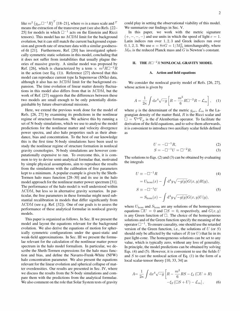
The linear halo bias predictions for the ΛCDM (black),QCDM (red) and R−2R (blue) models are shown in Fig. 5at a = 0.6, a = 0.8 and a = 1.0. The symbols show the sim-ulation results, which were obtained by measuring the ratio

b(k,M) =Phm(k,M)

Pk, (48)

where Pk is the total matter power spectrum and Phm(k,M)is the halo-matter cross spectrum for haloes of massM . Thesewere measured with the aid of a Delaunay Tessellation fieldestimator code [83, 84]. We measure the cross spectrum, in-stead of the halo-halo power spectrum, to reduce the amountof shot noise. The linear halo bias parameter is then given bythe large scale limit of b(k,M), i.e., b(M) = b(k 1,M).

11

FIG. 4. The cumulative mass function of dark matter haloes (upper panels) for the ΛCDM (black), QCDM (red) and R−2R (blue) models,at three epochs a = 0.6, a = 0.8 a = 1.0, as labelled. The lower panels show the difference w.r.t. the ΛCDM model results. The symbolsshow the simulation results, and the errorbars indicate twice the variance across the five realizations of the initial conditions. We have usedthe phase-space friends-of-friends Rockstar code [82] to build the halo catalogues (without subhalos) used to compute the halo abundances.We only show the results for haloes with mass M200 > 100 ×Mp ∼ 5 × 1011M/h, where Mp = ρm0L

3/Np is the particle mass in thesimulations. The lines correspond to the ST mass function of Eqs. (28) and (31) obtained using the fitted (solid lines) and the standard (dashedlines) (q, p) parameters listed in Table IV.

We only consider the halo mass bins for which b(k,M) hasclearly saturated to its asymptotic value on large scales.

The simulation results show that, within the errorbars, thelinear halo bias parameter for the three models is indistin-guishable at all epochs shown. This shows that the modifi-cations to gravity in the R−2R model are not strong enoughto modify substantially the way that dark matter haloes tracethe underlying density field. The ST formula, Eq. (33), repro-duces the simulations results very well. Note also that there islittle difference between the curves computed using the fitted(solid lines) and the standard (dashed lines) (q, p) parametersof Table IV. We conclude the same as in the case of the massfunction that, in the context of the R−2R model, there isno clear need to recalibrate the (q, p) parameters in order toreproduce the bias results from the simulations.

F. Halo concentration

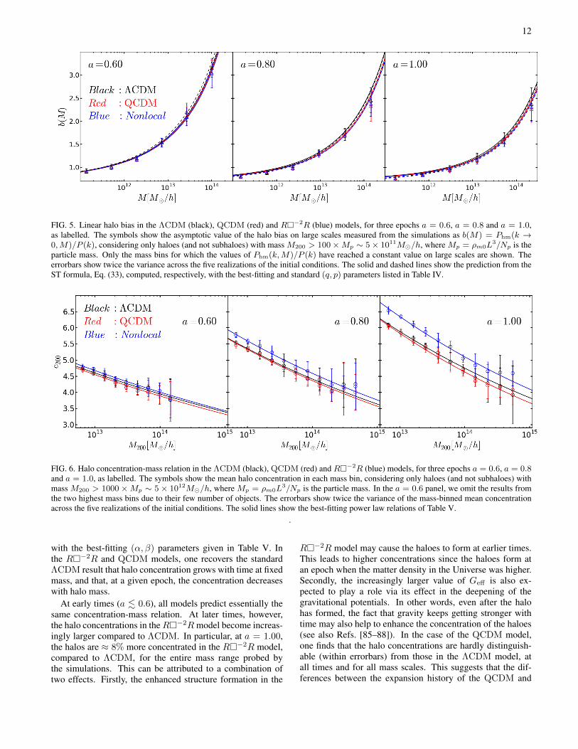
Figure 6 shows the halo concentration-mass relation for theΛCDM (black), QCDM (red) and R−2R (blue) models, ata = 0.60, a = 0.80 and a = 1.00. The symbols correspond tothe mean values of c200 identified in the same halo cataloguesused in Fig. 4. For all models, and at all epochs and mass

TABLE V. Concentration-mass relation best-fitting (α, β)parameters in the parametrization log10(c200) = α +βlog10

(M200/

[1012M/h

])to the simulation results at a = 0.6,

a = 0.8 and a = 1.0. The uncertainty in the values of α and β is∆α = ∆β = 0.001. These are the parameters that minimize thequantity

∑i(c

sims200 (Mi) − cparam

200 (Mi, α, β))2/(2∆csims200 (Mi))

2,where csims

200 (Mi) is the mean halo concentration measured from thesimulations, ∆csims

200 (Mi) is the variance of the mean across the fiverealizations and cparam

200 (Mi, α, β) is the concentration given by theparametrization. Here, the index i runs over the number of massbins.

Model a = 0.6 a = 0.8 a = 1.0(α, β) (α, β) (α, β)

ΛCDM (0.729,−0.066) (0.813,−0.084) (0.863,−0.093)QCDM (0.726,−0.068) (0.814,−0.087) (0.866,−0.100)R−2R (0.737,−0.067) (0.834,−0.086) (0.898,−0.095)

scales shown, one sees that the halo concentrations are wellfitted by the power law function (solid lines),

log10(c200) = α+ βlog10

(M200/

[1012M/h

]), (49)

12

FIG. 5. Linear halo bias in the ΛCDM (black), QCDM (red) and R−2R (blue) models, for three epochs a = 0.6, a = 0.8 and a = 1.0,as labelled. The symbols show the asymptotic value of the halo bias on large scales measured from the simulations as b(M) = Phm(k →0,M)/P (k), considering only haloes (and not subhaloes) with mass M200 > 100×Mp ∼ 5× 1011M/h, where Mp = ρm0L

3/Np is theparticle mass. Only the mass bins for which the values of Phm(k,M)/P (k) have reached a constant value on large scales are shown. Theerrorbars show twice the variance across the five realizations of the initial conditions. The solid and dashed lines show the prediction from theST formula, Eq. (33), computed, respectively, with the best-fitting and standard (q, p) parameters listed in Table IV.

FIG. 6. Halo concentration-mass relation in the ΛCDM (black), QCDM (red) and R−2R (blue) models, for three epochs a = 0.6, a = 0.8and a = 1.0, as labelled. The symbols show the mean halo concentration in each mass bin, considering only haloes (and not subhaloes) withmass M200 > 1000×Mp ∼ 5× 1012M/h, where Mp = ρm0L

3/Np is the particle mass. In the a = 0.6 panel, we omit the results fromthe two highest mass bins due to their few number of objects. The errorbars show twice the variance of the mass-binned mean concentrationacross the five realizations of the initial conditions. The solid lines show the best-fitting power law relations of Table V.

.

with the best-fitting (α, β) parameters given in Table V. Inthe R−2R and QCDM models, one recovers the standardΛCDM result that halo concentration grows with time at fixedmass, and that, at a given epoch, the concentration decreaseswith halo mass.

At early times (a . 0.6), all models predict essentially thesame concentration-mass relation. At later times, however,the halo concentrations in theR−2Rmodel become increas-ingly larger compared to ΛCDM. In particular, at a = 1.00,the halos are ≈ 8% more concentrated in the R−2R model,compared to ΛCDM, for the entire mass range probed bythe simulations. This can be attributed to a combination oftwo effects. Firstly, the enhanced structure formation in the

R−2R model may cause the haloes to form at earlier times.This leads to higher concentrations since the haloes form atan epoch when the matter density in the Universe was higher.Secondly, the increasingly larger value of Geff is also ex-pected to play a role via its effect in the deepening of thegravitational potentials. In other words, even after the halohas formed, the fact that gravity keeps getting stronger withtime may also help to enhance the concentration of the haloes(see also Refs. [85–88]). In the case of the QCDM model,one finds that the halo concentrations are hardly distinguish-able (within errorbars) from those in the ΛCDM model, atall times and for all mass scales. This suggests that the dif-ferences between the expansion history of the QCDM and

13

ΛCDM models (cf. Fig. 2) are not large enough to have animpact on the formation time of the haloes. Once the haloeshave formed in these two models, one can think as if the clus-tering inside these haloes decouples from the expansion. As aresult, and since the gravitational strength is the same (cf. Ta-ble II), one sees no significant differences in the concentrationof the haloes from the QCDM and ΛCDM simulations.

G. Nonlinear matter power spectrum

Figure 7 shows our results for the nonlinear matter powerspectrum. The power spectrum from the simulations was mea-sured using the POWMES code [89]. The solid (dashed) linesshow the halo model prediction obtained using Eq. (25) withthe fitted (standard) (q, p) parameters of Table IV. The dottedlines show the predictions obtained using linear theory. Next,we discuss these results separately for large, intermediate andsmall length scales.

Large scales. On scales k . 0.1h/Mpc, the halo modelis dominated by the 2-halo term, which is practically indis-tinguishable from the linear matter power spectrum. This isbecause, in the limit in which k → 0, one has that

I(k) ∼∫

dM1

ρm0

dn(M)

dlnMblin(M) = 1, (50)

where we have used the fact that |u(k → 0,M)| → 1 andthe last equality holds by the definition of the ST mass func-tion and halo bias [31]. In fact, in the standard halo modelapproach, replacing P 2h

k by Pk,lin in Eq. (25) leads to prac-tically no difference. As a result, the agreement between thehalo model and the simulation results on large (linear) scalesis always guaranteed.

Intermediate scales. On scales 0.1h/Mpc . k . 1h/Mpc,the halo model underpredicts slightly the power spectrummeasured from the simulations, for all models and at allepochs shown. This is due to a fundamental limitation of thehalo model on these scales, which follows from some simpli-fying assumptions about the modelling of halo bias on theseintermediate scales (see e.g. Sec. IV.F of Ref. [32] for a sim-ple explanation). In fact, the so-called halofit model arises asan alternative to the halo model that is more accurate on theseintermediate scales [90–92]. Nevertheless, in terms of the rel-ative difference to ΛCDM, the halo model limitations cancelto some extent, which leads to a better agreement with thesimulation results. Focusing on a = 1.00, the halo model pre-dictions for the QCDM model reproduce very well the resultsfrom the simulations. The predictions for the R−2R model,although not as accurate as in QCDM, still provide a fair es-timate of the enhancement of the clustering power relative toΛCDM. For example, at k ≈ 1h/Mpc and a = 1.00, thesimulations show an increase of ≈ 11% in the power relativeto ΛCDM, whereas the halo model predicts an enhancementof ≈ 15%, which is similar. Finally, it is worth mentioningthat the performance of the halo model when ones uses thestandard (q, p) = (0.75, 0.30) values (dashed lines) is com-

parable to the case where one uses the values that best fit themass function results (solid lines).

Small scales. On scales of k & 1h/Mpc, the halo modelpredictions are dominated by the 1-halo term, whose agree-ment with the simulations becomes better than on intermedi-ate scales, especially at a = 1.00. There are still some visiblediscrepancies at a = 0.60, which are similar to those foundin Ref. [32] for Galileon gravity models. These discrepanciesare however likely to be related with some of the assumptionsmade in the halo model approach, namely that all matter in theUniverse lies within bound structures, which is not true in thesimulations. However, similarly to what happens on interme-diate scales, the halo model performs much better when onelooks at the relative difference w.r.t. ΛCDM. The predictionsobtained by using the standard (q, p) parameter values (dashedlines), although not as accurate as the results obtained by us-ing the fitted (q, p) values (solid lines), are still able to providea good estimate of the effects of the modifications to gravityin the R−2R model on the small-scale clustering power.

In the QCDM model, the relative difference w.r.t. ΛCDMbecomes smaller with increasing k. In particular, for k &10h/Mpc at a = 1.0, the clustering amplitude of these twomodels becomes practically indistinguishable. This result canbe understood with the aid of the halo model expression forthe 1-halo term, P 1h

k , (cf. Eq. (26)), which depends on thehalo mass function and concentration-mass relation. Firstly,one notes that for smaller length scales, the integral in P 1h

kbecomes increasingly dominated by the lower mass end ofthe mass function. Consequently, the fact that the mass func-tion of the QCDM model approaches that of ΛCDM at lowmasses (becoming even smaller for M . 5 × 1012M/h ata = 1.00), helps to explain why the values of ∆Pk/Pk,ΛCDM

decrease for k & 1h/Mpc. Secondly, according to Fig. 6,the halo concentrations are practically the same in the ΛCDMand QCDM models. In other words, this means that in-side small haloes (those relevant for small scales), matter isalmost equally clustered in these two models, which helpsto explain why ∆Pk/Pk,ΛCDM is compatible with zero fork & 10h/Mpc (Ref. [93] finds similar results for k-mouflagegravity models).

The same reasoning also holds for the R−2R model,which is why one can also note a peak in ∆Pk/Pk,ΛCDM

at k ∼ 1h/Mpc. However, in the case of the R−2Rmodel, the mass function is larger at the low-mass end and thehalo concentrations are also higher, compared to QCDM andΛCDM. These two facts explain why ∆Pk/Pk,ΛCDM doesnot decrease in the R−2R model, being roughly constant ata = 1.00 for k & 1h/Mpc. In particular, we have explic-itly checked that if one computes the halo model predictionsof the R−2R model, but using the concentration-mass re-lation of ΛCDM, then one fails to reproduce the values of∆Pk/Pk,ΛCDM on small scales. This shows that a good per-formance of the halo model on small scales is subject to aproper modelling of halo concentration, which can only beaccurately determined in N-body simulations.

14

FIG. 7. The nonlinear matter power spectrum (upper panels) in the ΛCDM (black), QCDM (red) and R−2R (blue) models, at three epochsa = 0.6, a = 0.8 and a = 1.0, as labelled. The lower panels show the different w.r.t. ΛCDM. The symbols show the simulation results,where the errorbars show twice the variance across the five realizations of the initial conditions. The solid lines show the halo model predictionobtained using Eq. (25), with the best-fitting (q, p) parameters listed in Table IV. The dashed lines show the power spectrum when usingthe standard ST (q, p) = (0.75, 0.30) parameter values. The dotted lines show the result from linear perturbation theory. These lines areindistinguishable in the upper panels.

H. Nonlinear velocity divergence power spectrum

Figure 8 shows the nonlinear velocity divergence powerspectrum, Pθθ,5 for the three models of Table II and fora = 0.60, a = 0.80 and a = 1.00. The computation wasdone by first building a Delaunay tessellation using the par-ticle distribution of the simulations [83, 84], and then inter-polating the density and velocity information to a fixed gridto measure the power spectra. The upper panels show that onscales k . 0.1h/Mpc, the results from the simulations of allmodels approach the linear theory prediction, which is givenby

P linearθθ = a2

(H

H0

)2

f2P lineark , (51)

where P lineark is the linear matter power spectrum and f =

dlnδlin/dlna. On smaller scales, the formation of nonlinearstructures tends to slow down the coherent (curl-free) bulk

5 Here, θ is the Fourier mode of the divergence of the peculiar physical ve-locity field v, defined as θ(~x) = ∇v(~x)/H0.

flows that exist on larger scales. This leads to an overall sup-pression of the divergence of the velocity field compared tothe linear theory result for scales k & 0.1h/Mpc, as shown inthe upper panels.

In the lower panels, the simulation results also agree withthe linear theory prediction for k . 0.1h/Mpc. On thesescales, the time evolution of the power spectrum of all modelsis scale independent and the relative difference encapsulatesthe modifications to the time evolution of P linear

k , H and f ,in Eq. (51). On smaller scales, the values of ∆P θθk /P θθk,ΛCDMdecay w.r.t. the linear theory result until approximately k =1h/Mpc. This suppression follows from the fact that theformation of nonlinear structures is enhanced in the QCDMand R−2R models, relative to ΛCDM (cf. Figs. 4 and 7).Hence, on these scales, the suppression in the velocity diver-gence caused by nonlinear structures is stronger in the QCDMand R−2R model, compared to ΛCDM. Finally, on scalesk & 2 − 3h/Mpc, the relative difference to ΛCDM growsback to values comparable to the linear theory prediction. Onthese scales, one does not expect haloes to contribute con-siderably to P θθk for two main reasons. First, as haloes viri-alize, the motion of its particles tends to become more ran-dom, which helps to reduce the divergence of the velocityfield there. Secondly, and perhaps more importantly, P θθk iscomputed from a volume-weighted field, and as a result, since

15

FIG. 8. The nonlinear peculiar velocity divergence power spectrum (upper panels) in the ΛCDM (black), QCDM (red) and R−2R (blue)models, for three epochs a = 0.6, a = 0.8 and a = 1.0, as labelled. The lower panels show the difference w.r.t. ΛCDM. The symbols showthe simulation results, where the errorbars show the variance across the five realizations of the initial conditions. The dashed lines only linkthe symbols to help the visualization. The dotted lines in the bottom panels show the prediction of linear perturbation theory.

haloes occupy only a small fraction of the total volume, theyare not expected to contribute significantly to the total velocitydivergence power spectrum. On the other hand, considerablecontributions may arise from higher-volume regions such asvoids, walls or filaments, where coherent matter flows exist.For instance, matter can flow along the direction of dark mat-ter filaments, or inside a large wall or void that is expanding(see e.g. [94–96]). These small scale flows are larger in theQCDM and R−2R models at a fixed time, as shown by thegrowth of the values of ∆P θθk /P θθk,ΛCDM on small scales.

On scales k & 2 − 3h/Mpc, one may find it odd that theQCDM model predicts roughly the same matter power spec-trum as ΛCDM (cf. Fig. 7), but has a different velocity diver-gence power spectrum. This has to do with the weight withwhich different structures contribute to Pk and P θθk . For in-stance, Pk is computed from a mass-weighted density field,and hence, it is dominated by the highest density peaks, whichare due to dark matter haloes. In other words, it is very insen-sitive to the behavior of the clustering of matter in voids, wallsor filaments due to their lower density. On the contrary, P θθk ,which is computed from a volume-weighted field, is forciblyless sensitive to dark matter haloes due to their low volumefraction. The values of P θθk are then mostly determined by thevelocity field inside voids, walls and filaments. These struc-tures are typically larger than haloes and therefore they aremore sensitive to the background expansion of the Universe.Consequently, they are more likely to be affected by modifi-

cations to H(a), compared to haloes which detach from theoverall expansion sooner. This can then explain the differ-ences in the sizes of the modifications to Pk and P θθk on smallscales in the QCDM model, relative to ΛCDM. To test thiswe have computed P θθk by artificially setting θ(~x) = 0 in re-gions where the density contrast exceeds δ = 50. This shouldroughly exclude the contribution from haloes to the values ofP θθk . We have found no visible difference w.r.t. the results ofFig. 8, which shows that the small scale behavior of the ve-locity divergence is not affected by what happens inside darkmatter haloes. We have performed the same calculation, butby setting θ(~x) = 0 whenever δ < 0, to exclude the contri-bution from voids. We have found that at a = 1, the relativedifference of QCDM to ΛCDM at k ∼ 10h/Mpc drops from∼ 9% (as in Fig. 8) to ∼ 7%. This seems to suggest that thedominant effect in the small scale behavior of P θθk comes fromwalls and/or filaments. The velocity divergence in these struc-tures is typically large (see e.g. Fig. 2 of Ref. [97]) and theyalso occupy a sizeable fraction of the total volume as well.A more detailed investigation of these results is beyond thescope of the present paper.

Focusing at a = 1, at k ∼ 10h/Mpc and relative toΛCDM, the velocity power spectrum in the R−2R modelis enhanced by ∼ 12%, and the matter power spectrum by∼ 15%. On large (linear) scales the same figures are ∼ 12%and ∼ 7%, respectively. The size of the modifications tothe matter and velocity divergence power spectrum are rather

16

similar, but the latter might be easier to measure as they aretypically less sensitive to assumptions about baryonic pro-cesses such as galaxy bias. As an example, redshift spacedistortions (RSD) [98–100] are sensitive to the boost of thevelocity field on large scales, and therefore can be used totest modified gravity models (see e.g. Refs. [77, 101]). Thework of Refs. [102, 103] illustrated how the velocity distribu-tion of infalling galaxies around massive clusters can be usedto detect modifications to gravity (see also [104]). More re-cently, Ref. [105] demonstrated that modified gravity modelscan leave particularly strong signatures in the velocity disper-sion of pairs of galaxies on a broad range of distance scales.The level of precision of the data from future observationalmissions should prove sufficient to disentangle the differencesdepicted in Fig. 8. Such a forecast study would involve run-ning simulations with better resolution and larger box sizes,and as such, we leave it for future work.

V. SUMMARY

We have studied the nonlinear regime of structure forma-tion in nonlocal gravity cosmologies using N-body simula-tions, and also in the context of the semi-analytical ellipsoidalcollapse and halo models. To the best of our knowledge, thisis the first time the nonlinear growth of structure in nonlocalcosmologies has been studied. In particular, we investigatedthe impact that the modifications to gravity in nonlocal mod-els have on the halo mass function, linear halo bias param-eters, halo concentrations and on the statistics of the densityand velocity fields of the dark matter.

The action or equations of motion of nonlocal gravitymodels are typically characterized by the inverse of thed’Alembertian operator acting on curvature tensors. Here, wefocused on the model of Refs. [26, 27], in which the standardEinstein-Hilbert action contains an extra term proportional toR−2R (cf. Eq. (1)). The constant of proportionality is fixedby the dark energy density today, and hence this model con-tains the same number of free parameters as ΛCDM, althoughit has no ΛCDM limit for the background dynamics or gravi-tational interaction.

Our goal was not to perform a detailed exploration of thecosmological parameter space in the R−2R model. Instead,for the R−2R model we used the same cosmological pa-rameters as ΛCDM (cf. Table I). In this way one isolates theimpact of the modifications to gravity from the impact of hav-ing different cosmological parameter values. Nevertheless,although a formal exploration of the parameter space in theR−2Rmodel is left for future work (see Ref. [48]), the com-parison presented in Fig. 1 suggests that the model fits theCMB temperature data as well as ΛCDM. Our main resultscan be summarized as follows:

• The expansion rate in the R−2R model is smaller thanin ΛCDM at late times, and the gravitational strength is en-hanced by a time-dependent factor (cf. Fig. 2). Both effectshelp to boost the linear growth of structure (cf. Fig. 2) andalso speed up the collapse of spherical matter overdensities

(cf. Fig. 3). In particular, at the present day, the amplitude ofthe linear matter (velocity divergence) power spectrum is en-hanced by ≈ 7% (≈ 12%) in the R−2R model, comparedto ΛCDM. These results are in agreement with Ref. [27]. Thecritical density for collapse today, δc(a = 1), is≈ 3% smallerin the R−2R model, relative to ΛCDM (cf Fig. 3). Forthese results, the modified expansion history plays the dom-inant role in driving the differences w.r.t. ΛCDM, comparedto the effect of the enhanced Geff .

•At late times (a > 0.6), the number density of haloes withmasses M & 1012M/h is higher in the R−2R model,compared to ΛCDM. The difference becomes more pro-nounced at the high-mass end of the mass function. In par-ticular, at a = 1, haloes with mass M ∼ 1014M/h are≈ 10% more abundant in the R−2R model than in ΛCDM.At M = 1012M/h this difference is only ≈ 2%. The ef-fects of the modified H(a) and Geff on the enhancement ofthe high-mass end of the mass function are comparable.

The ST mass function describes well the absolute values ofthe halo number densities as well as the relative differencesw.r.t. ΛCDM, for all of the epochs studied (cf. Fig. 4). Wefind that the use of the standard (q, p) = (0.75, 0.30) ST pa-rameter values provides a fair estimate of the modifications tothe mass function in the R−2R model. However, recalibrat-ing these parameters to the simulation results helps to improvethe accuracy of the fit (cf. Table IV).

• The linear halo bias parameter in the R−2R model isbarely distinguishable from that in ΛCDM for all masses andepochs studied (cf. Fig. 5). In other words, the modificationsto gravity in the R−2R model play a negligible role in theway dark matter haloes trace the underlying density field. TheST halo bias formula provides therefore a good description ofthe simulation results. There is also almost no difference be-tween the semi-analytical predictions for the bias computedusing the best-fitting and standard values for the (q, p) ST pa-rameters.

• The halo concentration-mass relation is well-fitted by apower law function (cf. Fig. 6), but with fitting parameters thatdiffer from those of ΛCDM (see Table V). For a . 0.6, theconcentration of the haloes in the R−2R model is roughlythe same as in ΛCDM, but it increases with time. In particu-lar, at a = 1.0 (a = 0.8) and for all masses, haloes are ≈ 8%(≈ 4%) more concentrated in the R−2R model, comparedto ΛCDM. This is likely to be mainly due to the enhancedGeff on small scales, which helps to make the gravitationalpotential continuously deeper inside the haloes. On the otherhand, the effects of the modifications to the expansion historyin the R−2R play a negligible role in changing the concen-tration of the haloes. This can be explained by the fact thatthe modifications to H(a) are small enough not to have a sig-nificant impact on the formation time of the haloes. Conse-quently, once the haloes form, they detach from the expansionof the Universe and no longer "feel" the dynamics of the back-ground.

17

• The modifications to gravity in the R−2R model leadonly to a modest enhancement of the clustering power. Forinstance, at a = 1.0 (a = 0.8) the amplitude of the non-linear matter power spectrum is never larger than ≈ 15%(≈ 10%) on all scales (cf. Fig. 7). These differences mightbe hard to disentangle using data from galaxy clustering giventhe known uncertainties in modelling galaxy bias. On smallscales, k & 1h/Mpc, the differences w.r.t. ΛCDM are com-pletely determined by the enhanced Geff , and not by the mod-ifications to H(a).

At a = 1.0, the halo model describes the simulation resultson large (k . 0.1h/Mpc) and small (k & 1h/Mpc) scalesvery well. On intermediate scales and also at earlier times,the performance becomes worse due to known limitations ofthe halo model [31, 32]. These follow from a number of ap-proximations in the derivation of the halo model formalism,which sacrifice some accuracy in favour of analytical con-venience. In terms of the relative difference w.r.t. ΛCDM,these limitations cancel out and the halo model describes thesimulation results reasonably well for all epochs and scales.Moreover, the performance of the halo model formulae in de-scribing the simulation results does not depend critically onthe fitting of the (q, p) parameters to the mass function. How-ever, we have checked that the good performance of the halomodel on small scales is subject to a correct modelling of thehalo-concentration mass relation, which can only be properlydetermined via N-body simulation.

• Similarly to the case of the matter power spectrum,the modifications in the R−2R model lead only to modestchanges in the amplitude of the nonlinear velocity divergencepower spectrum. In particular, at a = 1.0 (a = 0.8) the en-hancement relative to ΛCDM is kept below ≈ 12% (≈ 10%)on all scales. However, measurements of RSD and/or galaxyinfall dynamics are less subject to galaxy bias uncertainties,and therefore, might stand a better chance of distinguishingbetween these two models.

• The R−2R model possesses no screening mechanismto suppress the modifications to gravity on small scales. Asa result, Solar System tests of gravity can be used to con-strain the model. For example, the R−2R model predictsthat Geff/G ≈ 92× 10−13 yrs−1, which is incompatible withthe current bound from Lunar Laser Ranging experiments,Geff/G = (4± 9)×10−13 yr−1 [81]. The local time variationofGeff follows from the background evolution of the auxiliaryscalar field S, and it seems nontrivial to devise a mechanismthat can suppress it around massive objects or in high-densityregions [37, 38]. In this paper, we focused only on a partic-ular choice of cosmological parameters. As a result, it mightbe possible that certain parameter combinations can be madecompatible with Solar System tests, whilst still being able to

yield viable cosmological solutions. Nevertheless, it seemsclear that these tests should be taken into account in futureconstraint studies, as they might have the potential to rule outthese models observationally.

In conclusion, the R−2R model, although it has noΛCDM limit for the dynamics of the background and grav-itational interaction, exhibits changes of only a few percentin observables sensitive to the nonlinear growth of structure.Some of these effects are degenerate with baryonic mecha-nisms such as AGN feedback or galaxy bias, or even withmassive neutrinos [45, 106–108]. This makes it challengingto distinguish this model from ΛCDM, but the precision ofupcoming observational missions such as Euclid [109, 110],DESI [111] or LSST [112] should make this possible. Froman observational point of view, however, future nonlinear stud-ies are only warranted provided the model is able to fit suc-cessfully the CMB data from Planck (see Ref. [48]), in a waythat is also compatible with the constraints from Lunar LaserRanging experiments. The latter requirement might be hard tosatisfy due to the absence of a screening mechanism.

ACKNOWLEDGMENTS

We thank Philippe Brax, Marius Cautun, Yves Dirian, Ste-fano Foffa, Ruth Gregory, Nima Khosravi, Michele Mag-giore, Michele Mancarella, Alex Kehagias, Martin Kunz andPatrick Valageas for useful comments and discussions. Wealso thank Lydia Heck for invaluable numerical support. Thiswork was supported by the Science and Technology Facili-ties Council [grant number ST/L00075X/1]. This work usedthe DiRAC Data Centric system at Durham University, oper-ated by the Institute for Computational Cosmology on behalfof the STFC DiRAC HPC Facility (www.dirac.ac.uk). Thisequipment was funded by BIS National E-infrastructure cap-ital grant ST/K00042X/1, STFC capital grant ST/H008519/1,and STFC DiRAC Operations grant ST/K003267/1 andDurham University. DiRAC is part of the National E-Infrastructure. AB is supported by FCT-Portugal throughgrant SFRH/BD/75791/2011. BL is supported by the RoyalAstronomical Society and Durham University. WAH is sup-ported by the ERC Advanced Investigator grant of C. S.Frenk, COSMIWAY, and by the Polish National Science Cen-ter through grant DEC-2011/01/D/ST9/01960. The researchleading to these results has received funding from the Eu-ropean Research Council under the European Union’s Sev-enth Framework Programme (FP/2007-2013) / ERC GrantNuMass Agreement n. [617143]. This work has been par-tially supported by the European Union FP7 ITN INVISI-BLES (Marie Curie Actions, PITN- GA-2011- 289442) andSTFC.

[1] C. M. Will(2014), arXiv:1403.7377 [gr-qc][2] T. Clifton, P. G. Ferreira, A. Padilla, and C. Skordis,

Phys.Rept. 513, 1 (2012), arXiv:1106.2476 [astro-ph.CO][3] D. Huterer, D. Kirkby, R. Bean, A. Connolly, K. Dawson,

18

et al.(2013), arXiv:1309.5385 [astro-ph.CO][4] B. Jain, A. Joyce, R. Thompson, A. Upadhye, J. Battat,

et al.(2013), arXiv:1309.5389 [astro-ph.CO][5] A. Joyce, B. Jain, J. Khoury, and M. Trodden(2014),

arXiv:1407.0059 [astro-ph.CO][6] R. Woodard, Found.Phys. 44, 213 (2014), arXiv:1401.0254

[astro-ph.CO][7] S. Deser and R. Woodard, Phys.Rev.Lett. 99, 111301 (2007),

arXiv:0706.2151 [astro-ph][8] C. Deffayet and R. Woodard, JCAP 0908, 023 (2009),

arXiv:0904.0961 [gr-qc][9] S. Deser and R. Woodard, JCAP 1311, 036 (2013),

arXiv:1307.6639 [astro-ph.CO][10] S. Nojiri and S. D. Odintsov, Phys.Lett. B659, 821 (2008),

arXiv:0708.0924 [hep-th][11] S. Jhingan, S. Nojiri, S. Odintsov, M. Sami, I. Thongkool,

et al., Phys.Lett. B663, 424 (2008), arXiv:0803.2613 [hep-th][12] T. Koivisto, Phys.Rev. D77, 123513 (2008), arXiv:0803.3399

[gr-qc][13] T. S. Koivisto, Phys.Rev. D78, 123505 (2008),

arXiv:0807.3778 [gr-qc][14] E. Elizalde, E. O. Pozdeeva, and S. Y. Vernov, Phys. Rev. D

85, 044002 (Feb. 2012), arXiv:1110.5806 [astro-ph.CO][15] E. Elizalde, E. O. Pozdeeva, and S. Y. Vernov, Classical and

Quantum Gravity 30, 035002 (Feb. 2013), arXiv:1209.5957[astro-ph.CO]

[16] S. Park and S. Dodelson, Phys. Rev. D 87, 024003 (Jan. 2013),arXiv:1209.0836 [astro-ph.CO]

[17] S. Dodelson and S. Park(2013), arXiv:1310.4329 [astro-ph.CO]

[18] M. Maggiore, Phys.Rev. D89, 043008 (2014),arXiv:1307.3898 [hep-th]

[19] S. Foffa, M. Maggiore, and E. Mitsou, Int.J.Mod.Phys. A, toappear(2014), arXiv:1311.3435 [hep-th]

[20] A. Kehagias and M. Maggiore, JHEP, to appear(2014),arXiv:1401.8289 [hep-th]

[21] S. Nesseris and S. Tsujikawa(2014), arXiv:1402.4613 [astro-ph.CO]

[22] M. Jaccard, M. Maggiore, and E. Mitsou, Phys.Rev. D88,044033 (2013), arXiv:1305.3034 [hep-th]

[23] S. Foffa, M. Maggiore, and E. Mitsou, Phys.Lett. B733, 76(2014), arXiv:1311.3421 [hep-th]

[24] L. Modesto and S. Tsujikawa, Phys.Lett. B727, 48 (2013),arXiv:1307.6968 [hep-th]

[25] P. G. Ferreira and A. L. Maroto, Phys.Rev. D88, 123502(2013), arXiv:1310.1238 [astro-ph.CO]

[26] M. Maggiore and M. Mancarella, Phys.Rev. D90, 023005(2014), arXiv:1402.0448 [hep-th]

[27] Y. Dirian, S. Foffa, N. Khosravi, M. Kunz, and M. Maggiore,JCAP 1406, 033 (2014), arXiv:1403.6068 [astro-ph.CO]

[28] R. K. Sheth and G. Tormen, Mon.Not.Roy.Astron.Soc. 308,119 (1999), arXiv:astro-ph/9901122 [astro-ph]

[29] R. K. Sheth, H. Mo, and G. Tormen,Mon.Not.Roy.Astron.Soc. 323, 1 (2001), arXiv:astro-ph/9907024 [astro-ph]

[30] R. K. Sheth and G. Tormen, Mon.Not.Roy.Astron.Soc. 329,61 (2002), arXiv:astro-ph/0105113 [astro-ph]

[31] A. Cooray and R. K. Sheth, Phys.Rept. 372, 1 (2002),arXiv:astro-ph/0206508 [astro-ph]

[32] A. Barreira, B. Li, W. A. Hellwing, L. Lombriser,C. M. Baugh, and S. Pascoli, JCAP 4, 029 (Apr. 2014),arXiv:1401.1497

[33] S. Capozziello, E. Elizalde, S. Nojiri, and S. D. Odintsov,Phys.Lett. B671, 193 (2009), arXiv:0809.1535 [hep-th]

[34] N. Koshelev, Grav.Cosmol. 15, 220 (2009), arXiv:0809.4927[gr-qc]

[35] T. S. Koivisto, AIP Conf.Proc. 1206, 79 (2010),arXiv:0910.4097 [gr-qc]

[36] A. O. Barvinsky, Phys.Rev. D85, 104018 (2012),arXiv:1112.4340 [hep-th]

[37] E. Babichev, C. Deffayet, and G. Esposito-Farese,Phys.Rev.Lett. 107, 251102 (2011), arXiv:1107.1569[gr-qc]

[38] R. Kimura, T. Kobayashi, and K. Yamamoto, Phys. Rev. D 85,024023 (Jan. 2012), arXiv:1111.6749 [astro-ph.CO]

[39] P. Ade et al. (Planck Collaboration)(2013), arXiv:1303.5075[astro-ph.CO]

[40] P. Ade et al. (Planck Collaboration)(2013), arXiv:1303.5076[astro-ph.CO]

[41] P. Ade et al. (Planck Collaboration)(2013), arXiv:1303.5077[astro-ph.CO]

[42] F. Beutler, C. Blake, M. Colless, D. H. Jones, L. Staveley-Smith, et al., Mon.Not.Roy.Astron.Soc. 416, 3017 (2011),arXiv:1106.3366 [astro-ph.CO]

[43] N. Padmanabhan, X. Xu, D. J. Eisenstein, R. Scalzo, A. J.Cuesta, et al., Mon.Not.Roy.Astron.Soc. 427, 2132 (2012),arXiv:1202.0090 [astro-ph.CO]

[44] L. Anderson, E. Aubourg, S. Bailey, D. Bizyaev, M. Blan-ton, et al., Mon.Not.Roy.Astron.Soc. 427, 3435 (2013),arXiv:1203.6594 [astro-ph.CO]

[45] A. Barreira, B. Li, C. Baugh, and S. Pascoli(2014),arXiv:1406.0485 [astro-ph.CO]

[46] A. Lewis, http://camb.info/[47] A. Barreira, B. Li, C. M. Baugh, and S. Pascoli, Phys.Rev.

D86, 124016 (2012), arXiv:1208.0600 [astro-ph.CO][48] Y. Dirian, S. Foffa, M. Kunz, M. Maggiore, and V. Pettorino,

in preparation[49] A. Barreira, B. Li, C. M. Baugh, and S. Pascoli, JCAP 1311,

056 (2013), arXiv:1308.3699 [astro-ph.CO][50] W. H. Press and P. Schechter, Astrophys. J. 187, 425 (Feb.

1974)[51] M. Maggiore and A. Riotto, Astrophys. J. 717, 515 (Jul. 2010),

arXiv:0903.1250 [astro-ph.CO][52] A. Nicolis, R. Rattazzi, and E. Trincherini, Phys. Rev. D 79,

064036 (2009)[53] A. De Felice and S. Tsujikawa, Phys.Rev.Lett. 105, 111301

(2010), arXiv:1007.2700 [astro-ph.CO][54] C. Deffayet, S. Deser, and G. Esposito-Farese, Phys.Rev. D80,

064015 (2009), arXiv:0906.1967 [gr-qc][55] H. Mo and S. D. White, Mon.Not.Roy.Astron.Soc. 282, 347

(1996), arXiv:astro-ph/9512127 [astro-ph][56] J. N. Fry and E. Gaztanaga, Astrophys.J. 413, 447 (1993),

arXiv:astro-ph/9302009 [astro-ph][57] J. F. Navarro, C. S. Frenk, and S. D. White, Astrophys.J. 490,

493 (1997), arXiv:astro-ph/9611107 [astro-ph][58] J. S. Bullock, T. S. Kolatt, Y. Sigad, R. S. Somerville, A. V.

Kravtsov, et al., Mon.Not.Roy.Astron.Soc. 321, 559 (2001),arXiv:astro-ph/9908159 [astro-ph]

[59] A. F. Neto, L. Gao, P. Bett, S. Cole, J. F. Navarro, et al.,Mon.Not.Roy.Astron.Soc. 381, 1450 (2007), arXiv:0706.2919[astro-ph]

[60] A. V. Maccio’, A. A. Dutton, and F. C. d. Bosch(2008),arXiv:0805.1926 [astro-ph]

[61] F. Prada, A. A. Klypin, A. J. Cuesta, J. E. Betancort-Rijo, andJ. Primack(2011), arXiv:1104.5130 [astro-ph.CO]

[62] J. Khoury and A. Weltman, Phys.Rev.Lett. 93, 171104 (2004),arXiv:astro-ph/0309300 [astro-ph]

[63] J. Khoury and A. Weltman, Phys.Rev. D69, 044026 (2004),

19

arXiv:astro-ph/0309411 [astro-ph][64] B. Li and G. Efstathiou, Mon.Not.Roy.Astron.Soc. 421, 1431

(2012), arXiv:1110.6440 [astro-ph.CO][65] R. Teyssier, Astron.Astrophys. 385, 337 (2002), arXiv:astro-

ph/0111367 [astro-ph][66] B. Li, G.-B. Zhao, R. Teyssier, and K. Koyama, JCAP 1201,

051 (2012), arXiv:1110.1379 [astro-ph.CO][67] E. Puchwein, M. Baldi, and V. Springel(2013),

arXiv:1305.2418 [astro-ph.CO][68] C. Llinares, D. F. Mota, and H. A. Winther(2013),

arXiv:1307.6748 [astro-ph.CO][69] H. Oyaizu, Phys.Rev. D78, 123523 (2008), arXiv:0807.2449

[astro-ph][70] G.-B. Zhao, B. Li, and K. Koyama, prd 83, 044007 (Feb.

2011), arXiv:1011.1257 [astro-ph.CO][71] W. A. Hellwing, B. Li, C. S. Frenk, and S. Cole,

Mon.Not.Roy.Astron.Soc. 435, 2806 (Nov. 2013),arXiv:1305.7486 [astro-ph.CO]

[72] A.-C. Davis, B. Li, D. F. Mota, and H. A. Winther, Astrophys.J. 748, 61 (Mar. 2012), arXiv:1108.3081 [astro-ph.CO]

[73] C. Llinares and D. F. Mota(2013), arXiv:1312.6016 [astro-ph.CO]

[74] K. C. Chan and R. Scoccimarro, PRD 80, 104005 (Nov. 2009),arXiv:0906.4548 [astro-ph.CO]

[75] F. Schmidt, Phys.Rev. D80, 043001 (2009), arXiv:0905.0858[astro-ph.CO]

[76] B. Li, G.-B. Zhao, and K. Koyama, JCAP 1305, 023 (2013),arXiv:1303.0008 [astro-ph.CO]

[77] M. Wyman, E. Jennings, and M. Lima, Phys.Rev. D88, 084029(2013), arXiv:1303.6630 [astro-ph.CO]

[78] A. Barreira, B. Li, W. A. Hellwing, C. M. Baugh, and S. Pas-coli, JCAP 2013, 027 (2013), arXiv:1306.3219 [astro-ph.CO]

[79] B. Li, A. Barreira, C. M. Baugh, W. A. Hellwing, K. Koyama,et al. JCAP11, 012 (2013), arXiv:1308.3491 [astro-ph.CO]

[80] H. A. Winther and P. G. Ferreira(2014), arXiv:1403.6492[astro-ph.CO]

[81] J. G. Williams, S. G. Turyshev, and D. H. Boggs,Phys.Rev.Lett. 93, 261101 (2004), arXiv:gr-qc/0411113 [gr-qc]

[82] P. S. Behroozi, R. H. Wechsler, and H.-Y. Wu, Astrophys.J.762, 109 (2013), arXiv:1110.4372 [astro-ph.CO]

[83] M. C. Cautun and R. van de Weygaert, ArXiv e-prints(May2011), arXiv:1105.0370 [astro-ph.IM]

[84] W. E. Schaap and R. van de Weygaert, A&A 363, L29 (Nov.2000), arXiv:astro-ph/0011007

[85] W. A. Hellwing and R. Juszkiewicz, Phys. Rev. D 80, 083522(Oct. 2009), arXiv:0809.1976

[86] W. A. Hellwing, S. R. Knollmann, and A. Knebe, MNRAS408, L104 (Oct. 2010), arXiv:1004.2929 [astro-ph.CO]

[87] W. A. Hellwing, Annalen der Physik 522, 351 (Mar. 2010),arXiv:0911.0573 [astro-ph.CO]

[88] W. A. Hellwing, M. Cautun, A. Knebe, R. Juszkiewicz, andS. Knollmann, J. Cosmology Astropart. Phys. 10, 012 (Oct.2013), arXiv:1111.7257 [astro-ph.CO]

[89] S. Colombi, A. H. Jaffe, D. Novikov, and C. Pichon(2008),

arXiv:0811.0313 [astro-ph][90] R. Smith et al. (Virgo Consortium), Mon.Not.Roy.Astron.Soc.

341, 1311 (2003), arXiv:astro-ph/0207664 [astro-ph][91] R. Takahashi, M. Sato, T. Nishimichi, A. Taruya, and

M. Oguri, Astrophys.J. 761, 152 (2012), arXiv:1208.2701[astro-ph.CO]

[92] G.-B. Zhao, Astrophys.J.Suppl. 211, 23 (2014),arXiv:1312.1291 [astro-ph.CO]

[93] P. Brax and P. Valageas(2014), arXiv:1403.5424 [astro-ph.CO]

[94] M. Cautun, R. van de Weygaert, B. J. T. Jones, andC. S. Frenk, Mon.Not.Roy.Astron.Soc. 441, 2923 (Jul. 2014),arXiv:1401.7866

[95] M. Cautun, R. van de Weygaert, and B. J. T. Jones,Mon.Not.Roy.Astron.Soc. 429, 1286 (Feb. 2013),arXiv:1209.2043 [astro-ph.CO]

[96] N. I. Libeskind, Y. Hoffman, and S. Gottlöber,Mon.Not.Roy.Astron.Soc. 441, 1974 (Jul. 2014),arXiv:1310.5706

[97] B. Li, W. A. Hellwing, K. Koyama, G.-B. Zhao, E. Jennings,and C. M. Baugh, Mon.Not.Roy.Astron.Soc. 428, 743 (Jan.2013), arXiv:1206.4317 [astro-ph.CO]

[98] R. Scoccimarro, Phys.Rev. D70, 083007 (2004), arXiv:astro-ph/0407214 [astro-ph]

[99] E. Jennings, C. M. Baugh, and S. Pascoli,Mon.Not.Roy.Astron.Soc. 410, 2081 (Jan. 2011),arXiv:1003.4282 [astro-ph.CO]

[100] E. Jennings, Mon.Not.Roy.Astron.Soc. 427, L25 (Nov. 2012),arXiv:1207.1439 [astro-ph.CO]

[101] E. Jennings, C. M. Baugh, B. Li, G.-B. Zhao, and K. Koyama,mnras 425, 2128 (Sep. 2012), arXiv:1205.2698 [astro-ph.CO]

[102] T. Y. Lam, T. Nishimichi, F. Schmidt, and M. Takada, Physi-cal Review Letters 109, 051301 (Aug. 2012), arXiv:1202.4501[astro-ph.CO]

[103] T. Y. Lam, F. Schmidt, T. Nishimichi, and M. Takada,Phys.Rev. D88, 023012 (2013), arXiv:1305.5548 [astro-ph.CO]

[104] Y. Zu, D. Weinberg, E. Jennings, B. Li, and M. Wyman(2013),arXiv:1310.6768 [astro-ph.CO]

[105] W. A. Hellwing, A. Barreira, C. S. Frenk, B. Li, and S. Cole,Phys.Rev.Lett. 112, 221102 (2014), arXiv:1401.0706 [astro-ph.CO]

[106] M. Baldi, F. Villaescusa-Navarro, M. Viel, E. Puchwein,V. Springel, et al.(2013), arXiv:1311.2588 [astro-ph.CO]

[107] J. Shim, J. Lee, and M. Baldi(2014), arXiv:1404.3639 [astro-ph.CO]

[108] A. Barreira, B. Li, C. Baugh, and S. Pascoli(2014),arXiv:1404.1365 [astro-ph.CO]

[109] R. Laureijs et al. (EUCLID Collaboration)(2011),arXiv:1110.3193 [astro-ph.CO]

[110] L. Amendola et al. (Euclid Theory Working Group)(2012),arXiv:1206.1225 [astro-ph.CO]

[111] M. Levi et al. (DESI collaboration)(2013), arXiv:1308.0847[astro-ph.CO]

[112] LSST Dark Energy Science Collaboration, ArXiv e-prints(Nov. 2012), arXiv:1211.0310 [astro-ph.CO]