Nonlinear simulation of tumor growth

Digital Object Identifier (DOI):10.1007/s00285-002-0174-6

J. Math. Biol. 46, 191–224 (2003) Mathematical Biology

Vittorio Cristini · John Lowengrub · Qing Nie

Nonlinear simulation of tumor growth

Received: 1 May 2002 / Revised version: 26 August 2002 /Published online: 18 December 2002 – c© Springer-Verlag 2002

Abstract. We study solid tumor (carcinoma) growth in the nonlinear regime using bound-ary-integral simulations. The tumor core is nonnecrotic and no inhibitor chemical speciesare present. A new formulation of the classical models [18,24,8,3] is developed and it isdemonstrated that tumor evolution is described by a reduced set of two dimensionless pa-rameters and is qualitatively unaffected by the number of spatial dimensions. One parameterdescribes the relative rate of mitosis to the relaxation mechanisms (cell mobility and cell-to-cell adhesion). The other describes the balance between apoptosis (programmed cell-death)and mitosis. Both parameters also include the effect of vascularization.

Our analysis and nonlinear simulations reveal that the two new dimensionless groupsuniquely subdivide tumor growth into three regimes associated with increasing degrees ofvascularization: low (diffusion dominated, e.g., in vitro), moderate and high vascularization,that correspond to the regimes observed in vivo. We demonstrate that critical conditionsexist for which the tumor evolves to nontrivial dormant states or grows self-similarly (i.e.,shape invariant) in the first two regimes. This leads to the possibility of shape control andof controlling the release of tumor angiogenic factors by restricting the tumor volume-to-surface-area ratio. Away from these critical conditions, evolution may be unstable leadingto invasive fingering into the external tissues and to topological transitions such as tumorbreakup and reconnection. Interestingly we find that for highly vascularized tumors, whilethey grow unbounded, their shape always stays compact and invasive fingering does notoccur. This is in agreement with recent experimental observations [30] of in vivo tumorgrowth, and suggests that the invasive growth of highly-vascularized tumors is associated tovascular and elastic anisotropies, which are not included in the model studied here.

1. Introduction

Tumor growth is a fundamental scientific problem and has received considerableattention by the mathematics community (see for example the recent review papers[1,9,2]). Here we focus on a continuum-scale description and pose the problem interms of conservation laws for the nutrient and tumor-cell concentrations, using anew formulation of an existing model [18,7,14]. This model describes evolution

V. Cristini, J. Lowengrub: School of Mathematics, and Department of Chemical Engineeringand Materials Science, University of Minnesota, Minneapolis MN 55455.

Current address: Department of Biomedical Engineering, and Department of Mathematics,University of California at Irvine, Irvine CA 92697. e-mail:[email protected];[email protected].

Q. Nie: Department of Mathematics, University of California at Irvine, Irvine CA 92697.e-mail: [email protected].

Key words or phrases: Tumor growth – Linear stability analysis – Self-similarity – Bound-ary-integral simulations

192 V. Cristini et al.

of avascular and vascularized tumors, but not the angiogenetic transition betweenthe two.

The tumor is treated as an incompressible fluid and tissue elasticity is neglected.Cell-to-cell adhesive forces are modeled by a surface tension at the tumor-tissueinterface. The growth of tumor mass is governed by a balance between cell mitosisand apoptosis (programmed cell-death). The rate of mitosis depends on the con-centration of nutrient and inhibitor chemical species, that obey diffusion-reactionequations in the tumor volume. The bulk source of chemical species is the blood.The concentration of capillaries in the tumor is assumed to be uniform as are theconcentrations of chemical species in the external tissues. In this paper we focus onthe case of nonnecrotic tumors (i.e., Phase I tumors) [7] with no inhibitor chemicalspecies. These conditions apply to small-sized tumors, or when the nutrient con-centrations in the blood and in the external tissues are high. We anticipate that sucha model should over-predict growth away from these conditions.

We present a new formulation of the mathematical model and we study tu-mor growth using boundary-integral simulations in the nonlinear regime to explorecomplex tumor morphologies. To our knowledge, these are the first fully nonlinearsimulations of a continuum model of tumor growth, and represent a step towardsthe development of a computer simulator of cancer, as will be discussed in moredetail in the Conclusions. We note that there has been recent work on cellular auto-mata-based simulations of tumor growth (e.g. see [19] and the references therein).Our new formulation demonstrates that tumor evolution is described by a reducedset of two parameters that characterize families of solutions. The parameter G de-scribes the relative rate of mitosis to the relaxation mechanisms (cell mobility andcell-to-cell adhesion). The parameter A describes the balance between apoptosisand mitosis. Both parameters also include the effect of vascularization. Our analy-sis reveals that tumor evolution is qualitatively unaffected by the number of spatialdimensions. Thus, here we focus our nonlinear simulations on 2D tumor geome-tries. Our study reveals that the two new dimensionless groups uniquely subdividetumor growth into three regimes associated with increasing degrees of vasculariza-tion: low (diffusion dominated, e.g., in vitro), moderate and high vascularization,that correspond to the regimes observed in in vivo experiments. We demonstrate thatcritical conditions exist for which the tumor evolves to nontrivial dormant statesor grows self-similarly (i.e., shape-invariant) in the first two regimes in the fullnonlinear system. Explicit examples of these behaviors are given using nonlinearsimulations. The existence of non-trivial dormant states was recently proved [13],but no examples of such states were given.

The self-similar behavior described here is analogous to that recently found indiffusional crystal growth [12], and leads to the possibility of shape control and ofcontrolling the release of tumor angiogenic factors by restricting the tumor volume-to-surface-area ratio. This could restrict angiogenesis during growth. Away fromthese critical conditions, evolution may lead to invasive fingering into the externaltissues and to topological transitions such as tumor breakup and reconnection. In-terestingly we find that, in the high-vascularization regime, while the tumor growsunbounded the tumor shape always stays compact and invasive fingering does notoccur. This is in agreement with recent experimental observations [30] of in vivo

Nonlinear simulation of tumor growth 193

tumor growth in a isotropic sponge-like matrix, and suggests that the invasivegrowth of highly-vascularized tumors is associated to vascular and elastic aniso-tropies, which are not included in the model investigated here.

In Sect. 2, our new formulation for nonnecrotic tumors is presented, analyticresults for radially symmetric tumors are revisited and the regimes of growth areidentified. Our linear analysis in two and three dimensions is presented in Sect.2.3. In Sect. 2.3.1, self-similar tumor evolution is investigated. Nonlinear simula-tions are presented in Sect. 4. Our conclusions and directions for future work arein Sect. 5.

2. Problem formulation and linear analysis

2.1. New formulation

The classical mathematical model [18,24,8,3] describing the evolution of nonne-crotic tumors in the absence of inhibitor chemical species is summarized in Appen-dix A. It is shown that the model system considered has only one intrinsic lengthscale: the diffusional length LD , and has three intrinsic time scales correspondingto the relaxation rate λR (associated to LD , cell mobility and cell-to-cell adhesion),the characteristic mitosis rate λM and the apoptosis rate λA. By using algebraicmanipulations, it can be shown that the dimensional problem stated in Appendix Acan be reformulated in terms of two nondimensional decoupled problems:

∇2� − � = 0,(1)

(�)� = 1;and

∇2p = 0,(2)

(p)� = κ − A G(x · x)�

2d,

in a d–dimensional tumor. Here, space and time have been normalized with theintrinsic scales LD and λ−1

R , the interface � separates the tumor volume from theexternal tissue, and the variables � and p represent a modified nutrient concen-tration and a modified pressure (see Appendix A for their definitions). The tumorsurface � (of local total curvature κ) is evolved using the normal velocity

V = −n · (∇p)� + G n · (∇�)� − A Gn · (x)�

d, (3)

where n is the outward normal to � and x is position in space. The instantaneousproblem stated above has only two dimensionless parameters:

G = λM

λR

(1 − B) ,

(4)A = λA/λM − B

1 − B.

194 V. Cristini et al.

The former describes the relative strength of cell mitosis to the relaxation mecha-nisms, and the latter describes the relative strength of cell apoptosis and mitosis.The effect of vascularization is in the parameter B defined in Appendix A. Notethat in the context of steady solutions, the parameter A is related to the parameter� introduced in [7] by A = 3�.

We define the rescaled rate of change of tumor volume H = ∫�

dxd as the massflux J = d

dtH = ∫

�V dxd−1. By using (1a)–(2a) we obtain from (3):

J = −G

∫

�

� dxd − A G H. (5)

2.2. Regimes of growth

In order to identify the regimes of growth, we consider evolution of a tumor thatremains radially symmetric. The interface � is an infinite cylinder for d = 2 ora sphere for d = 3, with radius R(t). All the variables have only r–dependence,where r is the polar coordinate. Equations (1)–(2) have the nonsingular solutions

�(r, t) =

I0(r)

I0(R), d = 2,

(sinh(R)

R

)−1 sinh(r)

r, d = 3,

(6)

and p(r, t) = (d − 1)R−1 − AGR2/(2d). Note that p(r, t) ≡ p(R, t), i.e., p isuniform across the tumor volume.

From equation (3) the evolution equation for the tumor radius R is:

dR

dt= V = −AG

R

d+ G

I1(R)

I0(R), d = 2.

1

tanh(R)− 1

R, d = 3.

(7)

Note that for a radially symmetric tumor, |G| rescales time and it can be shownthat V = G − AGR for d = 1, where R is defined for d = 1 as the instantaneousposition of the interface, with R(0) = 0. In all dimensions, unbounded growth(R → ∞) occurs if and only if AG ≤ 0. The growth velocity is plotted for d = 2in figure 1. Note that, for d = 3, the results are qualitatively similar and were re-ported in figure 9 in [7], although in the framework of the original formulation thegrowth regimes had not been identified. The figure is included here to identify thegrowth regimes. For given A, evolution from initial condition R(0) = R0 occursalong the corresponding curve. Three regimes are identified, and the behavior isqualitatively unaffected by the number of spatial dimensions d.

1. Low vascularization: G ≥ 0 and A > 0 (i.e., B < λA/λM ). Note that thespecial case of avascular growth (B = 0) belongs to this regime. Evolution ismonotonic and always leads to a stationary state R∞, that corresponds to theintersection of the curves in figure 1 with the dotted line V = 0. This behav-ior is in agreement with the experimental observations of in vitro diffusional

Nonlinear simulation of tumor growth 195

0 1 2 3 4 5 6 7 8 9 10−1

−0.8

−0.6

−0.4

−0.2

0

0.2

0.4

0.6

0.8

1

0.751

0.5

0.25

0−0.25

−0.5−0.75

−1

A =

R

VG

Fig. 1. Rescaled rate of growth G−1V from equation (7) as a function of rescaled tumorradius R for radially symmetric tumor growth and d = 2; A labelled.

growth [17] of multicell avascular spheroids to a dormant steady state [26,35].In the experiments, however, the tumors always develop a necrotic core whichfurther stabilizes their growth [6].

2. Moderate vascularization: G ≥ 0 and A ≤ 0 (i.e., 1 > B ≥ λA/λM ). Un-bounded growth occurs from any initial radius R0 > 0. The growth tends toexponential for A < 0 with velocity V → −AGR/d as R → ∞, and to linearfor A = 0 with velocity V → G as R → ∞.

3. High vascularization: G < 0 (i.e., B > 1). Growth (V > 0) may occur, de-pending on the initial radius, for A > 0, and is always unbounded; for A < 0(for which cell apoptosis is dominant: λA/λM > B), the evolution is alwaysto the only stationary solution R∞ = 0. This stationary solution may also beachieved for A > 0.

The stationary radius R∞ is independent of G, and is solution of V = 0 withV from equation (7). The stationary radius has limiting behaviors

R∞ → d A−1, A → 0,(8)

R∞ → d12 (d + 2)

12 (1 − A)

12 , A → 1,

where R∞ vanishes. Note that the limit A → 1 corresponds to λA → λM . Ford = 1 the stationary radius is R∞ = A−1 identically.

196 V. Cristini et al.

The pressure PC (see Appendix A) at the center of the tumor (r ≡ 0) is obtainedfrom equation (54b):

PC

(γ /LD)= (d − 1)/R + G − A G R2/(2d) − G

{1/I0(R), d = 2,

R/ sinh(R), d = 3,(9)

which has the asymptotic behavior PC (γ /LD)−1 → −AGR2/(2d) as R → ∞,indicating that if the tumor grows unbounded (AG ≤ 0) the pressure at the centeralso does (unless A = 0). This is a direct consequence of the absence of a necroticcore in this model. In a real system, the increasing pressure may itself contribute tonecrosis [27–29]. It is known (see, for example, [9]) that tumor cells continuouslyreplace the loss of cell volume in a tumor’s core because of necrosis, thus main-taining pressure finite. For d = 1 we define PC as the limit of P as R → −∞, andit can be shown that PC (γ /LD)−1 = G.

2.3. Linear analysis

We consider a perturbation of the spherical tumor interface �:

R(t) + δ(t)

{eilθ , d = 2,

Yl,m(θ, φ), d = 3,(10)

where δ is the dimensionless perturbation size and Yl,m is a spherical harmonic,where l and θ are polar wavenumber and angle, and m and φ azimuthal wavenumberand angle.

By solving the system of equations (1)–(3) in the presence of a perturbed in-terface we obtain the evolution equation (7) for the unperturbed radius R and theevolution equation for the perturbation size δ:

δ−1 dδ

dt

=

l

(J

2πR2 + A G

)

− A G

2

+G −(

J

2πR+ A G

R

2

)Il−1(R)

Il(R)− l

(l2 − 1

)

R3 − G I1(R)

R I0(R), d = 2,

G − A G − (l + 2) J

4πR3 − l(l − 1)(l + 2)

R3 , d = 3, (11)

where the dimensionless flux

J = 2π (d − 1) Rd−1 V + O (δ/R)2 , (12)

with V given by (7). Note that the linear evolution of the perturbation is inde-pendent of the azimuthal wavenumber m and there is a critical mode lc such thatperturbations grow for l < lc and decay for l > lc. The critical mode dependson the parameters A, G and the evolving radius R. This agrees with the linear

Nonlinear simulation of tumor growth 197

analyses presented in [18,7,5] for the special case where the unperturbed con-figuration is stationary (i.e. R constant). Also, for d = 1 it can be shown that

δ−1 ddt

δ = −l3 − G

((l2 + 1

) 12 − 1

)

+ AG (lR − 1).

During unbounded growth, AG ≤ 0 and perturbations decay to zero for d =1, 2 since δ−1 d

dtδ → lAGR < 0 for d = 1 and δ−1 d

dtδ → (l − 1)AG/2 < 0 for

d = 2, as R → ∞. For d = 3, δ−1 ddt

δ → 0, as R → ∞, for A = −3(l − 1)−1,and perturbations grow (decay) for A larger (smaller) than this value.

2.3.1. Shape evolution and conditions for self-similarityHere, we characterize the evolution of the perturbed shape using the shape factorδ/R (following Ref. [12]), governed by

(δ/R)−1 d

dt(δ/R) = δ−1 dδ

dt− J

2π (d − 1) Rd. (13)

Thus, whend

dt(δ/R) = 0

the tumor shape does not change in time and the evolution is linearly self-similar(sometimes also referred to as neutral stability). This condition divides regimes ofstable (δ/R → 0) and unstable (|δ/R| → ∞) growth.

Let us investigate conditions for which the tumor grows unbounded but self-sim-ilarly, thus maintaining its shape. This should have implications for angiogenesis, ortumor vascularization. It is known that angiogenesis occurs as tumor angiogeneticfactors are released within the tumor, and migrate to nearby vessels triggering thechemotaxis of endothelial cells and thus the formation of a network of blood vesselsthat finally penetrate the tumor providing unlimited supply of nutrients and thustypically resulting in malignancy. Assuming the flux of angiogenic factors to beproportional to the tumor/tissue interface area, and the rate of production of angio-genic factors to be proportional to the tumor volume, we conclude that self-similarevolution divides tumor growth in two categories: one (stable growth) character-ized by a decrease of the area-to-volume ratio during growth thus hampering orpreventing angiogenesis, the other (unstable growth) characterized by an increaseof the area-to-volume ratio and thus favoring angiogenesis.

In Sect. 4.3 the possibility of shape control, by “tuning” the parameter conditionsto impose self-similar growth, will be investigated in detail. Here we investigatethe possibility of self-similar evolution using constant parameters in the limit asthe effective tumor radius R → ∞.

The asymptotic behavior of the flux J as R → ∞ is, from (7) and (12), J →−2π (d − 1) AGRd/d . Note that if the tumor grows unbounded then AG ≤ 0. Ford = 3, it is easily shown from (11) and (13) that (δ/R)−1 d

dt(δ/R) → G (1 + Al/3)

as R → ∞ and thus there exists a critical

Al = −3l−1, (14)

198 V. Cristini et al.

such that for A = Al we obtain

d

dt(δ/R) → 0 as R → ∞,

and the growing tumor tends to self-similar (shape invariant) evolution. Under con-stant parameter conditions, unbounded growth that tends to self-similar is possibleonly in the moderate-vascularization regime characterized by G > 0 and A < 0.For A > Al the perturbation grows unbounded with respect to the growing un-perturbed radius; for A < Al it decays to zero. In the high-vascularization regime(G < 0), unbounded growth (A > 0) is always stable.

For d = 2 the perturbation always decays to zero thus leading to stable un-bounded growth, since (δ/R)−1 d

dt(δ/R) → AGl/2 as R → ∞ for A �= 0. Thus

in particular self-similar long-time behavior during growth with constant parame-ters is a peculiarity of three dimensions only. Moreover, in two dimensions unstable(bounded) growth is possible only in the low-vascularization regime. In Sect. 4.3and inAppendix B we demonstrate that unstable and self-similar unbounded growthare possible, both for d = 2 and d = 3, by varying the dimensionless parametersA and G in time. Interestingly, these results reveal that growth for d = 2 and 3 hasthe same qualitative features.

3. Numerical method

3.1. Boundary integral formulation

In two dimensions, the interface � ≡ ∂�(t) is represented by a planar curve,with arclength s. From potential theory, � can be expressed using a double-layerpotential ν:

� (x) = −(2π)−1∫

�

ν′ n′ · ∇K0(∣∣x′ − x

∣∣) ds′, (15)

where n is the outward normal of �, the prime indicates quantities evaluated atthe position s′ on the interface, and the Green’s function is −(2π)−1K0, whereK0 is the modified Bessel function [10]. Let � be parameterized counterclock-wise by x(α) ≡ (x(α), y(α)) with the arbitrary parameter α ∈ [0, 2π ] such that

ds = (x2α + y2

α

) 12 dα. Taking the limit of equation (15) for x → x (s) ∈ �, the

boundary condition (1b) becomes a second-kind Fredholm integral equation on theboundary �:

ν(α)

2+

∫ 2π

0ν(α′) K (

α, α′) dα′ = 1 (16)

where

K (α, α′) = (

(x(α′) − x(α)) yα′ − (y(α′) − y(α)) xα′) K1(r)

2πr(17)

with r = ((x(α′) − x(α))2 + (y(α′) − y(α))2

) 12 , and a subscript indicates differ-

entiation. In deriving equation (16), we have used

d

drK0(r) = −K1(r). (18)

Nonlinear simulation of tumor growth 199

The kernel K has a logarithmic singularity at α = α′:

K (α, α′) = L1

(α, α′) ln

(

4 sin2 α − α′

2

)

+ L2(α, α′) , (19)

where L1 and L2 are analytic and periodic [23,11]:

L1(α, α′) = ((

x(α′) − x(α))

yα′ − (y(α′) − y(α)

)xα′

) I1(r)

4πr, (20)

L2(α, α′) = K (

α, α′) − L1(α, α′) ln

(

4 sin2 α − α′

2

)

, (21)

and I1(r) is the modified Bessel function. Note that

L2(α, α) = 1

4π

yααxα − xααyα

x2α + y2

α

. (22)

For the computation of p, a dipole-layer representation [25] is used with the di-pole-layer potential η. We recast equation (2b) in terms of a second-kind Fredholmintegral equation on the boundary � [15,21]:

− η(α)

2+ 1

2π

∫ 2π

0η(α′)

(x(α) − x(α′))yα′ − (y(α) − y(α′))xα′

(x(α) − x(α′))2 + (y(α) − y(α′))2 dα′

= κ − AGx(α)2 + y(α)2

4. (23)

The normal velocity V in equation (3) requires the evaluation of the normalderivatives n · ∇� and n · ∇p. We first discuss the former. The normal derivativeof the double layer potential can be written in terms of a single layer potential S

[22,10]:

n · ∇� (s) = d

dsS (νs) − n (s) · S (nν) , (24)

where

S (P) ≡ − (2π)−1∫

�

P(s′) K0

(∣∣x (s) − x(s′)∣∣) ds′, (25)

for any vector (or scalar) P. In (25), the function K0 has a logarithmic singularityat s = s′, and a decomposition similar to equation (19) can be performed.

The normal derivative of p is computed using the Dirichlet-Neumann map [25,15,21]:

n · ∇p (α) = 1

2π

∫ 2π

0ηα′

(x(α) − x(α′)) yα′ + (y(α) − y(α′)) xα′

(x(α) − x(α′))2 + (y(α) − y(α′))2 dα′, (26)

where the principal value of the integral is taken.

200 V. Cristini et al.

3.2. Surface representation and quadrature

We discretize the planar curve describing the surface � using N marker points,with parametrization αj = jh, h = 2π/N , N is a power of 2. For an analytic andperiodic function L1, the following quadrature formula is spectrally accurate [16]:

∫ 2π

0L1

(αi, α

′) ln

(

4 sin2 αi − α′

2

)

dα′ ≈2n−1∑

j=0

w|j−i|L1(αi, αj ) (27)

for αi = πi/n, i = 0, ..., 2n − 1, n = N/2, where

wj = −2π

n

n−1∑

m=1

1

mcos

mjπ

n− (−1)jπ

n2 , j = 0, ..., 2n − 1. (28)

We use the standard composite trapezoidal rule for the integral involving thekernel L2, yielding spectral accuracy.

To compute S (P) we employ the same computational strategy for (24) as usedfor the kernel L1. The derivatives d/ds in (24) are approximated using Fast-Fou-rier-Transform spectral derivatives. As a result, n · ∇� is discretized with spectralaccuracy.

In equations (23) and (26), the integrals are calculated using the alternating-point trapezoidal quadrature also yielding spectral accuracy [34].

Using the collocation method with the quadrature rules described above, we re-duce the boundary integral equations (16) and (23) to a dense linear system, whichis then solved using an iterative solver GMRES [31]. Following [32,21], a 15thorder Fourier filter is used to reduce aliasing errors. Moreover, during a simulation,marker points are added by multiples of 2 (using trigonometric interpolation) whenthe amplitude of the Nyquist frequency (N/2) exceeded the tolerance for solvingthe integral equation.

3.3. Surface evolution

To evolve the tumor surface � (t), we follow [32,21] and use the tangent-angle/areaformulation in a scaled arclength frame defined by

ds = L

2πdα, (29)

where L(t) is the length of the tumor surface. This implies that the collocationpoints are equally spaced in arclength. Accordingly, we evolve the tumor surfaceusing the tangential velocity

T (α) = α

2π

∫ 2π

0θα′V ′dα′ −

∫ α

0θα′V ′dα′, (30)

where θ (α) is the angle between the tangent to the tumor surface and the x-axis:

xα = L

2πcos θ yα = L

2πsin θ, (31)

Nonlinear simulation of tumor growth 201

and V is the normal velocity. The length L(t) and the area H(t) of the tumor arerelated by

H(t) = L2

8π2

∫ 2π

0

∫ α

0sin

(θ − θ ′) dα′ dα. (32)

The evolution of the tumor surface is reposed in terms of θ(α, t), H(t), and thecentroid (xc, yc). The time-derivatives are

θ (α, t) = 2π

L(Vα + T θα) , H (t) =

∫

�

V ds, (33)

xc(t) = 1

H

(∫

�

x V ds − xcH

)

, yc(t) = 1

H

(∫

�

y V ds − ycH

)

. (34)

It can be shown that from equations (1–3), for our problem xc = yc = 0. After atime step, the point positions on the surface are reconstructed using (31)–(32), withintegration constant determined from (34).

Following [32], we can show that, at small spatial scales,

V ∼(

2π

L

)2

H (θαα) (35)

where H(ξ) = (4π)−1∫ 2π

0 ξ ′ cot((α − α′)/2)dα′ is the Hilbert transformation forany scalar ξ . This demonstrates that an explicit time-stepping scheme has the high-order constraint �t ≤ (hL/2π)3, where �t and h are the temporal and spatial gridsizes. In [32] and later in [21], time stepping methods based on an integration factorand Crank-Nicholson discretizations have been developed to reduce the stabilityconstraint. In this paper, we use a Crank-Nicholson discretization and a O(�t)2

method based on an integration factor [32].

4. Results

4.1. Unstable growth

Here, we investigate unstable evolution in the low-vascularization (diffusion dom-inated) regime, characterized by G, A > 0, for d = 2 using nonlinear boundary-integral simulations. The linear analysis in Sect. 2.3.1 demonstrates that evolutionin the other regimes is stable for d = 2. In Figure 2, the evolution of the tumor sur-face from a nonlinear boundary-integral simulation with N = 1024 and �t = 10−3

(solid curve) is compared to the result of the linear analysis (dotted). In this caseA = 0.5, G = 20, and the initial shape of the tumor is

(x(α), y(α)) = (2 + 0.1 cos 2α) (cos α, sin α) . (36)

According to linear theory (formula (7) and figure 1), the tumor grows. The radiallysymmetric equilibrium radius R∞ ≈ 3.32. Mode l = 2 is linearly stable initially,and becomes unstable at R ≈ 2.29. The linear and nonlinear results in figure 2 areindistinguishable up to t = 1, and gradually deviate thereafter. Correspondingly, ashape instability develops and forms a neck.At t ≈ 1.9, the linear solution collapses

202 V. Cristini et al.

Fig. 2. Evolution of the tumor surface in the low-vascularization regime, for d = 2, A = 0.5,G = 20, and initial tumor surface as in equation (36). Dotted lines: solution from linear anal-ysis; solid: solution from a nonlinear calculation with time step �t = 10−3 and a number ofmarker points N = 1024, reset, after time t = 2.51, to �t = 10−4 and N = 2048.

suggesting pinch-off; the nonlinear solution is stabilized by the cell-to-cell adhesiveforces (surface tension) that resist the development of high negative curvatures inthe neck. This is not captured by the linear analysis. Instead of pinching off, asis predicted linear evolution, the nonlinear tumor continues to grow and developslarge bulbs that eventually reconnect thus trapping healthy tissue (shaded regionsin the last frame in Figure 2) within the tumor. The frame at t = 2.531 describes theonset of reconnection of the bulbs. We expect that reconnection would be affect-ed by diffusion of nutrient outside the tumor, which is not included in the modelused here. However, the predictions of the development of shape instabilities andof the capture of healthy tissue during growth are in agreement with experimentalobservations [33].

The accuracy of our nonlinear calculations is established by a resolution studyof the simulation shown in Figure 2. First, the spatial error is investigated by varyingthe number N of collocation points representing the tumor surface. In Figure 3, themaximal differences in the tumor surface between a simulation with N = 1024 and

Nonlinear simulation of tumor growth 203

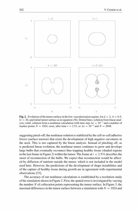
Fig. 3. Spatial resolution study for the case in figure 2: maximal differences between thesolution calculated using N = 1024 and other smaller N .

others with smaller N are plotted as functions of time. In all cases the time step is�t = 10−3. The tolerance for solving the integral equations for � and p is 10−10.At early times, the error is dominated by the tolerance in solving the equations;thus, the error decreases only slightly, from 10−8 to 10−9, as N increases. This isconsistent with the high-order accuracy of our discretization. The calculations forsmaller N stop at much earlier times than those for larger N due to the failure insolving the integral equations with the given tolerance. Clearly, the solution com-puted using N = 512 is accurate to 10−9, close to the tolerance 10−10, until thetumor surface is about to pinch (t ≈ 2.5).

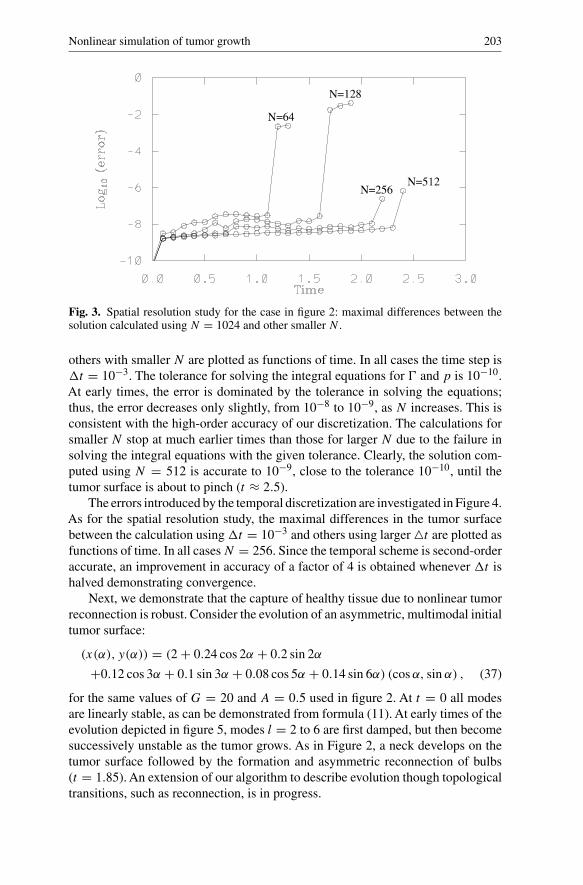
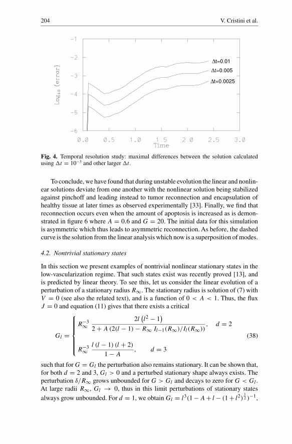
The errors introduced by the temporal discretization are investigated in Figure 4.As for the spatial resolution study, the maximal differences in the tumor surfacebetween the calculation using �t = 10−3 and others using larger �t are plotted asfunctions of time. In all cases N = 256. Since the temporal scheme is second-orderaccurate, an improvement in accuracy of a factor of 4 is obtained whenever �t ishalved demonstrating convergence.

Next, we demonstrate that the capture of healthy tissue due to nonlinear tumorreconnection is robust. Consider the evolution of an asymmetric, multimodal initialtumor surface:

(x(α), y(α)) = (2 + 0.24 cos 2α + 0.2 sin 2α

+0.12 cos 3α + 0.1 sin 3α + 0.08 cos 5α + 0.14 sin 6α) (cos α, sin α) , (37)

for the same values of G = 20 and A = 0.5 used in figure 2. At t = 0 all modesare linearly stable, as can be demonstrated from formula (11). At early times of theevolution depicted in figure 5, modes l = 2 to 6 are first damped, but then becomesuccessively unstable as the tumor grows. As in Figure 2, a neck develops on thetumor surface followed by the formation and asymmetric reconnection of bulbs(t = 1.85). An extension of our algorithm to describe evolution though topologicaltransitions, such as reconnection, is in progress.

204 V. Cristini et al.

Fig. 4. Temporal resolution study: maximal differences between the solution calculatedusing �t = 10−3 and other larger �t .

To conclude, we have found that during unstable evolution the linear and nonlin-ear solutions deviate from one another with the nonlinear solution being stabilizedagainst pinchoff and leading instead to tumor reconnection and encapsulation ofhealthy tissue at later times as observed experimentally [33]. Finally, we find thatreconnection occurs even when the amount of apoptosis is increased as is demon-strated in figure 6 where A = 0.6 and G = 20. The initial data for this simulationis asymmetric which thus leads to asymmetric reconnection. As before, the dashedcurve is the solution from the linear analysis which now is a superposition of modes.

4.2. Nontrivial stationary states

In this section we present examples of nontrivial nonlinear stationary states in thelow-vascularization regime. That such states exist was recently proved [13], andis predicted by linear theory. To see this, let us consider the linear evolution of aperturbation of a stationary radius R∞. The stationary radius is solution of (7) withV = 0 (see also the related text), and is a function of 0 < A < 1. Thus, the fluxJ = 0 and equation (11) gives that there exists a critical

Gl =

R−3∞

2l(l2 − 1

)

2 + A (2(l − 1) − R∞ Il−1(R∞)/Il(R∞)), d = 2

R−3∞

l (l − 1) (l + 2)

1 − A, d = 3

(38)

such that for G = Gl the perturbation also remains stationary. It can be shown that,for both d = 2 and 3, Gl > 0 and a perturbed stationary shape always exists. Theperturbation δ/R∞ grows unbounded for G > Gl and decays to zero for G < Gl .At large radii R∞, Gl → 0, thus in this limit perturbations of stationary states

always grow unbounded. For d = 1, we obtain Gl = l3(1 − A + l − (1 + l2)12 )−1,

Nonlinear simulation of tumor growth 205

Fig. 5. Evolution in the low-vascularization regime from a boundary-integral simulationwith d = 2, G = 20 and A = 0.5, and initial condition as in formula (37). The time stepfor the calculation is �t = 2 × 10−4. The number of marker points N = 512 initially, andis gradually increased to 2048 by the end of the simulation (t = 1.85) as required by thehighly deformed tumor surface.

which indicates that a nontrivial stationary solution may not exist, since Gl can benegative.

Let us next consider the nonlinear evolution for d = 2 of a mode l perturbationpredicted by the linear theory to be stationary. The value of G is equal to Gl , withR = R∞, given in Eq. (38).Although the perturbations are linearly stationary, thereis evolution due to nonlinearity. In figure 7 (top), the nonlinear evolution of severallinearly stationary shapes in the low-vascularization regime is shown through theirnonlinear perturbation size

δ/R0 = maxj

(|xj/R0|2 − 1

)1/2j = 1, N,

where the maximum is taken over all the computational nodes of the interface. Thecorresponding evolution of the tumor cross-sectional area in the x-y plane is shownin figure 7 (bottom). The linear steady shape corresponds to l = 4, A = 0.304,

206 V. Cristini et al.

t = 0 1

2.28 3

45.2

Fig. 6. Solid: nonlinear boundary-integral simulation of unstable growth of perturbation inthe low-vascularization regime; d = 2, G = 20, A = 0.6, initial and stationary radii R0 = 2and R∞ = 2.5771. Time is labeled. Dashed: linear result for same conditions.

G = G4 = 1.073. Initially, R0 = 6, and several initial perturbations are consid-ered: δ0/R0 = 0.01, 0.05, 0.1, 0.2. In addition, for each δ0/R0, several values ofG are considered. In figure 7, the solid curves correspond to the choice G = G4,the dotted curves to a value of G G4 and the dashed curves to a value ofG ≈ GNL

4 < G4, where GNL4 represents a nonlinear critical value, that depends

on the size of the perturbation, for which the numerical results predict evolution toa nontrivial nonlinear stationary state: δ/R becomes constant and non-zero. Here,we find only a numerical approximation to GNL

4 . For G > GNL4 perturbations are

nonlinearly unstable; for G < GNL4 they are stable and decay to zero (and the

undeformed configuration is steady).

The deviation G4 −GNL4 , for our numerical approximation to GNL

4 , is reportedin figure 8 (top) as a function of the limiting perturbation (δ/R)2∞ and demon-strates the effect of nonlinearity on the critical value of G. The corresponding areadeviation from the linear solution is shown in figure 8 (bottom).

Our results strongly suggest that for given l there exists a critical GNLl < Gl

such that for G = GNLl a nonlinear, nontrivial steady shape exists. Thus, nonlin-

earity is destabilizing for the stationary shapes. This is in contrast with the resultsobtained in section 4.1 where nonlinearity stabilizes the pinchoff predicted by lin-

Nonlinear simulation of tumor growth 207

0 5 10 15 20 25 30 35 40 45 50

10−2

10−1

Time

δ /R0

0 5 10 15 20 25 30 35 40 45 50110

115

120

125

130

135

140

Time

Area

Fig. 7. Top: time evolution of the perturbation size relative to a spherical tumor for d = 2,different initial l = 4 perturbations and A = 0.304. Solid: G = G4, Dotted: G G4,Dashed: G ≈ GNL

4 . Bottom: the corresponding evolution of the tumor area.

ear theory during unstable evolution. Finally, as expected, figure 8 indicates that thedeviation of GNL

l from the linear Gl is to the second order. For several perturbationsexamined, the initial (dashed curves) and steady nonlinear shapes (solid curves) aredepicted in figure 9.

208 V. Cristini et al.

0 0.002 0.004 0.006 0.008 0.01 0.012 0.014 0.016 0.018 0.020

0.05

0.1

0.15

0.2

0.25

0.3

0.35

0.4

(δ/R)2∞

G4−GNL

4

0 0.002 0.004 0.006 0.008 0.01 0.012 0.014 0.016 0.018 0.020

0.05

0.1

0.15

0.2

0.25

0.3

0.35

0.4

(δ/R)2∞

Area−Area0

Fig. 8. Top: The difference G4 −GNL4 versus the limiting steady nonlinear perturbation size

(δ/R)∞. Bottom: The corresponding area difference.

4.3. Self-similar evolution

Here we study self-similar evolution using linear analysis and nonlinear simula-tions, and we explore the possibility of controlling the shape of a tumor duringgrowth to take advantage of self-similar conditions and prevent growth of shape in-

Nonlinear simulation of tumor growth 209

−8 −6 −4 −2 0 2 4 6 8−8

−6

−4

−2

0

2

4

6

8

−8 −6 −4 −2 0 2 4 6 8−8

−6

−4

−2

0

2

4

6

8

−8 −6 −4 −2 0 2 4 6 8−8

−6

−4

−2

0

2

4

6

8

Fig. 9. The initial (dashed) and steady (solid) nonlinear tumor configurations for differentinitial perturbation amplitudes δ0/R0 = 0.01, 0.05, 0.2 corresponding to the data in figure7 with G ≈ GNL

4 .

stabilities. In figure 10 the evolution of a perturbation, predicted by linear analysis,during unbounded tumor growth (R → ∞) is examined in the moderate-vascular-ization regime characterized by G > 0 and A ≤ 0. As demonstrated from linearanalysis in Sect. 2.3.1, corresponding to d = 3 (solid lines) and A = Al the shapetends to become self-similar. For A > Al the perturbation grows unbounded withrespect to the unperturbed radius; for A < Al it decays to zero. For d = 2 (dashedlines) the perturbation always decays to zero. The behaviors as R → ∞ are

δ/R ∼{

R−l , d = 2,

R−(3A−1+l

), d = 3,

(39)

for A �= 0, and

δ/R ∼{

R−1, d = 2,

eR, d = 3,(40)

independently of l, for A = 0. Note that in this case V → G for both d = 2 and 3.

210 V. Cristini et al.

100

101

102

10−4

10−3

10−2

10−1

100

101

/R0

R

δ R/( )0

δ R/A4

A = =−3/4

−0.85

−3/4

08−

−0.65

0

Fig. 10. Rescaled growth ratio (δ/R) / (δ/R)0 as a function of rescaled radius R/R0 duringunbounded growth in the moderate-vascularization regime for d = 2 (dashed) and d = 3(solid); G = 1, l = 4, and A as labeled. The initial radius R0 = 10, except for the curved = 3, A = 0, for which R0 = 7. Asymptotic behaviors (dotted) from equations (39)–(40).

An analysis of the limit (δ/R)∞ of the shape factor δ/R as t → ∞ for d = 3and A = Al = −3/l corresponding to self-similar evolution as R → ∞ revealsthat the nontrivial limiting shape factor (δ/R)∞ → (δ/R)0 as R0 → ∞.

In the low-vascularization regime (G, A > 0) and in the high-vascularizationregime (G < 0) with A < 0, no unbounded growth occurs. In these regimes theperturbation may either grow or decay, and thus complicated tumor morphologiescan develop, as was illustrated by full nonlinear simulations in Sect. 4.1 in thelow-vascularization regime.

4.3.1. Time-dependent parameters

In experiments of in vitro [35] and in vivo [33] growth, the time scales that char-acterize prevascular or moderately vascular growth are relatively short (e.g., onemonth) and apoptosis can be neglected [33], i.e. λA = 0. Thus the dimensionlessparameter A becomes A = −B/ (1 − B). Therefore, it is possible to design anexperiment where the parameter A may be varied by changing B (through nutrientconcentrations in the blood, for example) while keeping the parameter G constantby adjusting the mitosis rate λM , for example through therapy. Analogously, it isalso possible to vary G while maintaining A constant. On longer time scales, apop-tosis is nonzero, and can be also controlled through therapy (e.g., radiation). Theseconsiderations and the following analysis reveal that, by varying the parameters ap-propriately, it should be possible to control the shapes of growing tumors therebypreventing the occurence of instabilities and invasive fingering.

Nonlinear simulation of tumor growth 211

One example of shape control is to maintain self-similar evolution duringgrowth by setting d

dt(δ/R) = 0 identically in equation (13). This can be achieved

by keeping G constant and varying A as a function of the unperturbed radius R by

A =

2(l2 − 1

)

G R3 + 2l−1(

I1 (R) Il−1 (R)

I0 (R) Il (R)− 1

)

− 2(

1 − 2l−1)

R−1 I1 (R) /I0 (R), d = 2,

3 (l + 2) (l − 1)

G R3 − 3l−1

+ 3(

1 + 3l−1)

R−2 (R/ tanh (R) − 1), d = 3.

(41)

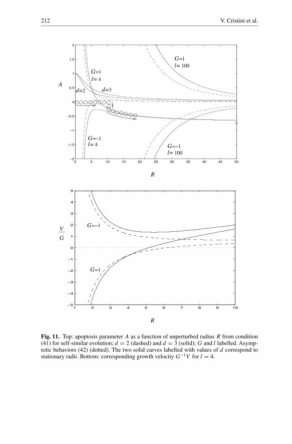
In figure 11 (top) the apoptosis parameter A(R) from Eq. (41) is shown ford = 2 (dashed lines) and d = 3 (solid). The growth velocity corresponding to self-similar evolution, obtained from (7) with A given by (41), is plotted in figure 11(bottom). The curves of A divide the plot into regions of stable growth and regionsof unstable growth of a given mode l. Figures 11 top and bottom indicate that inthe low-vascularization (diffusion-dominated) regime (G > 0, A > 0) self-similarevolution towards a stationary state is not possible for G constant (the stationarystates R∞ correspond to the intersection of curves (41) in figure 11 (top) with thecurves describing stationary radii). For instance, the growth velocity V < 0 for ini-tial radius R0 < R∞, and thus self-similar shrinkage of the tumor to zero occurs.On the other hand, for R0 > R∞, V > 0, and thus self-similar growth away fromthe stationary radius occurs. In the high-vascularization regime (G < 0), duringself-similar evolution the velocity V < 0. Thus self-similar shrinkage of a tumorfrom arbitrary initial condition to a point occurs, and self-similar unbounded growthis not possible.

Let us now focus on unbounded growth conditions: AG < 0. The limitingbehaviors as R → ∞ are A ≈ 2l−1R−1 > 0 for d = 2, and A ≈ −3l−1 +3

(1 + 3l−1

)R−1 < 0 for d = 3, and are independent of G. For G > 0 and A < 0

(moderate-vascularization regime), growth is stable for A < A(R) and unstableotherwise (note that A < A(R) always for d = 2); for G < 0 and A > 0 (highvascularization), growth is always stable since the stability condition is in this caseA > A(R) and A(R) < 0 as R → ∞. For d = 2, self-similar evolution remainsin the low-vascularization regime (A > 0), and does not occur in the moderate-vascularization regime; in contrast, for d = 3, a transition takes place into themoderate-vascularization regime (A becomes negative), and leads to unboundedself-similar growth. One can imagine an experiment in which an initially avasculartumor grows in the diffusion-dominated regime with G > 0 and A = 0. This corre-sponds to moving along the zero axis to the right, in figure 11, as illustrated by theopen circles. As the tumor grows by diffusion, angiogenesis occurs, and A becomesnegative. By adjusting A through the concentration of nutrient in the blood stream,while keeping G constant by adjusting the mitosis rate λM at the same time, one

212 V. Cristini et al.

0 5 10 15 20 25 30 35 40 45 50−2

−1.5

−1

−0.5

0

0.5

1

1.5

2

l=

l= 100

l= 100

4

=1

G=−1

G=−1

=1

l= 4

2d= d=3A

G

G

R

1 2 3 4 5 6 7 8 9 10−5

−4

−3

−2

−1

0

1

2

3

4

5

V

G

R

G=1

G=−1

Fig. 11. Top: apoptosis parameter A as a function of unperturbed radius R from condition(41) for self-similar evolution; d = 2 (dashed) and d = 3 (solid); G and l labelled. Asymp-totic behaviors (42) (dotted). The two solid curves labelled with values of d correspond tostationary radii. Bottom: corresponding growth velocity G−1V for l = 4.

Nonlinear simulation of tumor growth 213

can evolve the vascularized tumor along the curve A(R) that corresponds to self-similar growth in the moderate-vascularization regime, thus controlling the shapeand preventing invasive fingering. Correspondingly, the proliferation rate shouldbe varied as: (λM − λA)/λR = G (1 − A(R)). As l → ∞,

A →{

2(l2 − 1

)G−1R−3, d = 2,

3 (l + 2) (l − 1) G−1R−3, d = 3,(42)

and thus A > 0 and self-similar evolution in the low-vascularization regime be-comes possible at all radii (and it becomes forbidden in the moderate-vasculariza-tion regime) also for d = 3.

The apoptosis parameter for self-similar evolution with d = 1 is A =(

G−1l3 − 1 + (l2 + 1

) 12

)

(lR − 1)−1; note as a special case that, for G =

l−3(

(1 + l2

) 12 − 1

)

, A = 0 and unbounded self-similar growth occurs with con-

stant parameters. The behaviors described remain qualitatively unchanged for dif-ferent values of l.

To summarize, we found self-similar evolution, with the possiblity of shapecontrol, in all regimes with varying A and constant G. However, we discoveredthat in the low-vascularization regime, self-similar evolution to a steady state doesnot occur under these conditions. Similarly, self-similar unbounded growth in thehigh-vascularization regime does not occur. In Appendix B we examine the possi-bility of self-similar evolution to a steady-state in the low-vascularization regimeand of unbounded self-similar growth in the high vascularization regime by varyingG in addition to A.

4.3.2. Effect of nonlinearityWe now investigate the effect of nonlinearity on the self-similar evolution for d = 2predicted by the linear analysis.As discussed in section 4.3.1, self-similar evolutionrequires the time-dependent apoptosis parameter A = A(l, G, R) given in Eq. (41)and plotted in figure 11 (top). The radius R, used in the nonlinear simulation, isdetermined by the area of an equivalent circle: R = √

H/π . Examples of nonlinearself-similar evolution in the low-vascularization regime with l = 4 and G = 1 areshown in figure 12. In the top graph, the initial radius and perturbation are R0 = 7and δ0 = 0.3. Since the velocity V > 0, from figure 11 (bottom), the tumor growsand correspondingly A decreases. In the bottom graph, R0 = 4 and δ0 = 0.2; thecorresponding V < 0 indicating that the tumor shrinks (A increases). The solidcurves correspond to the nonlinear solution, at time t = 0 and at a later time, andthe dashed curves to the linear. The two are nearly indistinguishable revealing thatself-similar evolution is robust to nonlinearity for small perturbations.

In figure 13, the linear and nonlinear solutions are compared in the low-vascu-larization regime for l = 5, G = 1, A = A(l, G, R) and R0 = 4. Since V < 0,the tumors shrink and A increases. In the top figure, δ0 = 0.2 and in the bottomδ0 = 0.4. The results reveal that large perburbations are nonlinearly unstable andgrow, leading to a topological transition. In the last frame in figure 13 (bottom), the

214 V. Cristini et al.

-15

-10

-5

0

5

10

15

-15 -10 -5 0 5 10 15

-4

-3

-2

-1

0

1

2

3

4

-4 -3 -2 -1 0 1 2 3 4

Fig. 12. Top: self-similar nonlinear growth for R0 = 7 and δ0 = 0.3 (times t = 0 andt = 20 shown). Bottom: self-similar nonlinear shrinkage for R0 = 4 and δ0 = 0.2 (t = 0and t = 1.6 shown). The solid curves correspond to the nonlinear solution and the dashedcurves to the linear. In both cases, the evolution is in the low-vascularization regime withd = 2, l = 4 and G = 1, and the time-dependent A = A(l, G, R) given in Eq. (41) andplotted in figure 11 (top).

Nonlinear simulation of tumor growth 215

-4

-3

-2

-1

0

1

2

3

4

-4 -3 -2 -1 0 1 2 3 4

-4

-3

-2

-1

0

1

2

3

4

-4 -3 -2 -1 0 1 2 3 4

Fig. 13. Top: self-similar shrinkage for R0 = 4 and δ0 = 0.2 (t = 0 to 0.96 shown). Bottom:Unstable shrinkage for R0 = 4 and δ0 = 0.4 (t = 0 to 0.99). The solid curves correspondto the nonlinear solution and the dashed curves to the linear. In both cases, d = 2, G = 1,l = 5 and the evolution is in the low-vascularization regime. A = A(l, G, R) given in Eq.(41) and plotted in figure 11 (top).

216 V. Cristini et al.

-2

-1

0

1

2

-2 -1 0 1 2

-15

-10

-5

0

5

10

15

-15 -10 -5 0 5 10 15

Fig. 14. Nonlinear stable evolution in the high vascularization regime. Top: shrinkage withA = 0.2 and G = −5 (t = 0, 0.4, 0.8, 1.2 and 2.0 shown). Bottom: growth with A = 0.8and G = −5 (t = 0, 0.2, 0.5, 1.0, 1.5 and 2.3 shown). In both, the initial data is as in Eq.(36).

Nonlinear simulation of tumor growth 217

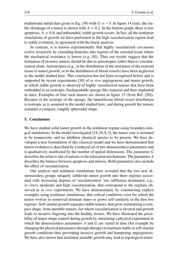
Fig. 15. HDMEC tumors seeded in biodegradable sponges and implanted in SCID micefrom [30]. The larger tumors overexpress the angiogenic factor Bcl-2 and are thus morehighly vascularized.

onset of pinch-off is evident. This can have important implications for therapy. Forexample, one can imagine an experiment in which a tumor is made to shrink bytherapy such that A is increased by increasing the apoptosis rate λA. Our exampleshows that a rapid decrease in size can result in shape instability leading to tumorbreak-up and the formation of microscopic tumor fragments that can enter the bloodstream through leaky blood vessels thus leading to metastases.

4.4. Evolution in the high vascularization regime

In the high-vascularization regime (G < 0), both shrinkage and growth of tumorsoccur. Shrinkage (A < 0) may be stable, self-similar and unstable. In contrast,unbounded growth (A > 0) is always characterized by a decay of the perturbationto zero with respect to the unperturbed radius and is thus stable for both d = 2and 3. In the nonlinear regime, we find that self-similar and unstable shrinkage arequalitatively very similar to that presented in figure 13 and therefore we do notpresent these results here. Instead, we present stable, nonlinear evolution from the

218 V. Cristini et al.

multimodal initial data given in Eq. (36) with G = −5. In figure 14 (top), the sta-ble shrinkage of a tumor is shown with A = 0.2. In the bottom graph, there is lessapoptosis, A = 0.8, and unbounded, stable growth occurs. In fact, all the nonlinearsimulations of growth we have performed in the high vascularization regime leadto stable evolution, in agreement with the linear analysis.

In contrast, it is known experimentally that highly vascularized carcinomaevolve invasively by extending branches into regions of the external tissue wherethe mechanical resistance is lowest (e.g. [9]). Thus our results suggest that theformation of invasive tumors should be due to anisotropies rather than to vascular-ization alone. Anisotropies (e.g., in the distribution of the resistance of the externaltissue to tumor growth, or in the distribution of blood vessels) have been neglectedin the model studied here. This conclusion has not been recognized before and issupported by recent experiments [30] of in vivo angiogenesis and tumor growth,in which stable growth is observed of highly vascularized tumors that have beenembedded in an isotropic, biodegradable sponge-like material and then implantedin mice. Examples of four such tumors are shown in figure 15 (from Ref. [30]).Because of the isotropy of the sponge, the tumor/tissue blood-vessel distributionis isotropic as is assumed in the model studied here, and during growth the tumorsmaintain a compact, roughly spheroidal shape.

5. Conclusions

We have studied solid tumor growth in the nonlinear regime using boundary-inte-gral simulations. In the model investigated [18,24,8,3], the tumor core is assumedto be nonnecrotic and no inhibitor chemical species to be present. We have de-veloped a new formulation of this classical model and we have demonstrated thattumor evolution is described by a reduced set of two dimensionless parameters andis qualitatively unaffected by the number of spatial dimensions. The parameter G

describes the relative rate of mitosis to the relaxation mechanisms. The parameter A

describes the balance between apoptosis and mitosis. Both parameters also includethe effect of vascularization.

Our analysis and nonlinear simulations have revealed that the two new di-mensionless groups uniquely subdivide tumor growth into three regimes associ-ated with increasing degrees of vascularization: low (diffusion dominated, e.g.,in vitro), moderate and high vascularization, that correspond to the regimes ob-served in in vivo experiments. We have demonstrated, by constructing explicitexamples using nonlinear simulations, that critical conditions exist for which thetumor evolves to nontrivial dormant states or grows self-similarly in the first tworegimes. Self-similar growth separates stable tumors, that grow maintaining a com-pact shape, from unstable tumors, for which vascularization is favored and growthleads to invasive fingering into the healthy tissues. We have illustrated the possi-bility of tumor shape control during growth by simulating a physical experiment inwhich the dimensionless parameters A and G are varied in time (for example bychanging the physical parameters through therapy) to maintain stable or self-similargrowth conditions thus preventing invasive growth and hampering angiogenesis.We have also shown that nonlinear unstable growth may lead to topological transi-

Nonlinear simulation of tumor growth 219

tions such as tumor breakup and reconnection with encapsulation of healthy tissue.Interestingly we have found that for highly vascularized tumors, while they growunbounded, their shape always stays compact and invasive fingering does not occur.This is in agreement with recent experimental observations [30] of in vivo tumorgrowth, and suggests that the invasive growth of highly-vascularized tumors is as-sociated to vascular and elastic anisotropies, which are not included in the modelwe have studied.

The work presented here demonstrates that nonlinear simulations are a pow-erful tool for understanding the phenomena that lead to growth of tumors. We areworking at the development of a three-dimensional computer simulator of a moresophisticated model of tumor growth, that includes the direct description of angio-genesis, and the effects of vascular and elastic (e.g., [20]) anisotropies that mayset preferred directions of growth and thus should be responsible for the invasivegrowth of maligant tumors. Angiogenesis is described by following the diffusionof tumor angiogenic factors through the tissues, and the chemotaxis of endothelialcells in response, leading to a nonuniform density of blood vessels. Such a sophis-ticated computer simulator should be useful for the scientific understanding of theconditions under which complex tumor morphologies develop during growth (suchas networks of blood vessels and shape instabilities), and also to help the designof targeted physical experiments in vitro or in vivo. Finally, this cancer simulatorshould find applications in a clinic environment, for example for testing differentcandidate therapies. As was only qualitatively illustrated in this paper, therapy willbe simulated by rigorously describing its effect on the physical parameters (such asmitosis and death rates) that characterize a tumor’s microenvironment. Simulationsof a specific patient’s reaction to each therapy can thus lead to the selection of themost promising therapies to be applied in vivo.

Appendix A

Governing equations

We consider a nonnecrotic tumor occupying a volume �(t). In the absence of in-hibitor chemical species, following [18,7,14], the quasi-steady diffusion equationfor the concentration σ(x, t) of nutrient is

0 = D∇2σ + �, (43)

where D is the diffusion constant, and � is the rate at which nutrient is added to �.The assumption of quasi-steady diffusion [7] is well supported by the considerationthat the tumor volume doubling time scale (e.g., one day) is typically much largerthat the diffusion time scale (≈ one minute).

The rate � incorporates all sources and sinks of nutrient in the tumor volume.Nutrient is supplied by the vasculature at a rate �B(σ, σB), where σB is the (uni-form) concentration in the blood. The rate of consumption of nutrient by the tumorcells is λ σ , with λ uniform. The blood-tissue transfer rate is assumed to be linear:

�B = −λB (σ − σB) , (44)

220 V. Cristini et al.

where λB is uniform. Thus, the rate � is given by

� = −λB (σ − σB) − λ σ. (45)

Modeling the tumor as an incompressible fluid, it follows that the velocity fieldu in � satisfies the continuity equation

∇ · u = λP , (46)

where λP is the cell-proliferation rate. We choose here the model

λP = bσ − λA, (47)

which is linear with respect to the nutrient concentration [7]: λA is the rate ofapoptosis and b and λA are assumed to be uniform.

The velocity is assumed to obey Darcy’s law [17]:

u = −µ∇P, (48)

where µ is the (constant) cell mobility and P(x, t) is the pressure inside �.The boundary condition for concentration at � ≡ ∂� is

(σ )� = σ∞, (49)

where σ∞ is the nutrient concentration outside the tumor volume, assumed to beuniform. This sets the characteristic mitosis rate to be

λM = bσ∞.

Pressure is assumed to satisfy the Laplace-Young boundary condition

(P )� = γ κ, (50)

where γ is the surface tension related to cell-to-cell adhesive forces, and κ is localtotal curvature. Finally, the normal velocity V = n · (u)� at the tumor boundary(with outward normal n) is

V = −µ n · (∇P)� . (51)

Dimensionless formulation

Equations (43) and (45) reveal that there is an intrinsic length scale

LD = D12 (λB + λ)−

12 , (52)

which for λB = 0 roughly estimates the stable size of an avascular tumor whendiffusion of nutrient and consumption balance. By nondimensionalizing lengthswith LD we obtain, from equations (48) and (50), an intrinsic relaxation time scaleλ−1

R corresponding to the rate

λR = µγL−3D (53)

Nonlinear simulation of tumor growth 221

2 4 6 8 10 12 14 16 18 200

0.2

0.4

0.6

0.8

1

1.2

1.4

1.6

1.8

2

G

R

V < 0

V > 0

5 6 7 8 9 100

0.1

0.2

0.3

0.4

0.5

0.6

R

A

V

Fig. 16. Top: growth parameter G from condition (41) for shape invariance, with V = 0and A(R) from Eq. (7) as a function of radius R; d = 2 (dashed) and d = 3 (solid); l = 4.Experiment of self-similar evolution between stationary states (dotted), with G imposed asa linear function of R. Bottom: apoptosis parameter A from (41), and growth velocity V , asa function of radius R during such experiment.

222 V. Cristini et al.

associated to the relaxation mechanisms cell mobility and surface tension. Theabove rate is used to nondimensionalize time.

Let us introduce the dimensionless parameters A and G defined in (4) and themodified concentration and pressure � and p so that

σ = σ∞ (1 − (1 − B)

(1 − �

)),

P = γ

LD

(p + (

1 − �)

G + A Gx · x2d

). (54)

The parameter

B = σB

σ∞λB

λB + λ(55)

represents the extent of vascularization.By algebraic manipulations it can be shown that equations (1) is obtained from

equations (43), (45) and (49). Equations (2) are obtained from (46)–(48) and (50).Finally, equation (3) is obtained from (51). In the main text of the paper, the barshave been dropped for simplicity.

Appendix B

Here we examine the possibility of self-similar evolution to a steady-state in thelow-vascularization regime and of unbounded self-similar growth in the high vas-cularization regime by varying G in addition to A. In figure 16 (top) the values ofgrowth parameter G as a function of radius R are plotted corresponding to nontrivialstationary states with a fixed tumor shape: d

dR(δ/R) = 0. In the high-vasculariza-

tion regime (G < 0), self-similar evolution occurs below the curves V = 0 infigure 16 (top), and thus V < 0 and self-similar unbounded growth remains for-bidden. Thus, unbounded growth in the high-vascularization is always stable evenfor variable A and G which is in agreement with recent experiments [30].

We consider then self-similar evolution between nontrivial stationary states inthe low-vascularization regime (G > 0). The dotted lines in figure 16 (top) repre-sent an experiment in which G is varied linearly between a stationary state R∞,1and a stationary state R∞,2 > R∞,1. In figure 16 (bottom), the correspondinggrowth velocities and time-dependent apoptosis parameters are shown. The figurereveals that during this experiment the growth velocity V > 0 and thus self-similarevolution is possible between the two stationary states. Other experimental pathsare possible, that lead to either growth or shrinkage of tumors to stationary states.The qualitative behaviors described are not affected by l.

Acknowledgements. V. Cristini and J. Lowengrub acknowledge Professor S. Ramakrishnanat the University of Minnesota for useful discussions, partial support from the NationalScience Foundation and the Minnesota Supercomputing Institute, and the hospitality of theInstitute for Mathematics and its Applications. V. Cristini also acknowledges the support ofthe MSI through a Reseach Scholar Award. Q. Nie acknowledges partial support from theNSF.

Nonlinear simulation of tumor growth 223

References

1. Adam, J.: General Aspects of Modeling Tumor Growth and Immune Response. In: ASurvey of Models on Tumor Immune Systems Dynamics, J. Adam and N. Bellomo Editors(Birkhauser, Boston 1996) 15–87

2. Bellomo, N., Preziosi, L.: Modelling and Mathematical Problems Related to TumorEvolution and Its Interaction with the Immune System. Mathl. Comput. Modelling 32,413–452 (2000)

3. Byrne, H.M.: The importance of intercellular adhesion in the development of carcino-mas. IMA J. Math. Med. Biol. 14, 305–323 (1997)

4. Byrne, H.M.: A weakly nonlinear analysis of a model of avascular solid tumour growth.J. Math. Biol. 39, 59–89 (1999)

5. Byrne, H.M., Chaplain, M.A.J.: Free boundary value problems associated with the gro-wth and development of multicellular spheroids. Eur. J. Appl. Math. 8, 639–658 (1997)

6. Byrne, H.M., Chaplain, M.A.J.: Growth of Nonnecrotic Tumors in the Presence andAbsence of Inhibitors. Mathl. Biosci. 135, 187–216 (1996)

7. Byrne, H.M., Chaplain, M.A.J.: Growth of Nonnecrotic Tumors in the Presence andAbsence of Inhibitors. Mathl. Biosci. 130, 151–181 (1995)

8. Byrne, H.M., Chaplain, M.A.J.: Modelling the role of cell-cell adhesion in the growthand development of carcinomas. Mathl. Comput. Modelling 24, 1–17 (1996)

9. Chaplain, M.A.J.: Avascular growth, Angiogenesis and Vascular growth in SolidTumours: The Mathematic Modelling of the Stages of Tumour Development. Mathl.Comput. Modelling 23, 47–87 (1996)

10. Colton, D., Kress, R.: Integral Equation Methods in Scattering Theory (Wiley-Inter-science, New York 1983)

11. Colton, D., Kress, R.: Inverse Acroustic and Electromagnetic Scattering Theory(Springer, Berlin 1992)

12. Cristini, V., Lowengrub, J.: Three-dimensional crystal growth. I. Linear analysis andself-similar evolution. J. Crystal Growth 240, 267–276 (2002)

13. Friedman, A., Reitich, F.: On the existence of spatially patterned dormant malignanciesin a model for the growth of non-necrotic vascular tumors. Math. Models Meth. Appl.Sci. 11, 601–625 (2001)

14. Friedman, A., Reitich, F.: Analysis of a mathematical model for the growth of tumors.J. Math. Biol. 38, 262 (1999)

15. Greenbaum, A., Greengard, L., McFadden, G.B.: Laplace’s equation and theDirichlet-Neumann map in multiply connected domains, J. Comp. Phys. 105, 267 (1993)

16. Greenbaum, A., Greengard, L., McFadden, G.B.: On the numerical solution of a hyper-singular integral equation in scattering theory, J. Comp.Appl. Math. 61, 345–360 (1995)

17. Greenspan, H.P.: Models for the Growth of a Solid Tumor by diffusion. Stud. Appl.Math. LI,4, 317–340 (1972)

18. Greenspan, H.P.: On the growth and stability of cell cultures and solid tumors. J. Theor.Biol. 56, 229–242 (1976)

19. Kansal, A.A., Torquato, S., Harsh IV, G.R., Chiocca, E.A., Deisboeck, T.S: Simulatedbrain tumor growth dynamics using a 3-D cellular automaton, J. Theor. Biol. 203,367–382 (2000)

20. Jones, A.F., Byrne, H.M., Gibson, J.S., Dold, J.W.: A mathematical model of the stressinduced during avascular tumour growth. J. Math. Biol. 40, 473–499 (2000)

21. Leo, P., Lowengrub, J., Nie, Q. Microstructural Evolution in Orthotropic Elastic Media,J. Comp. Phys. 157, 44–88 (2000)

22. Maue, A.: Uber die Formulierung eines allgemeinen Beugungsproblems durch eineIntegralgleichung, Zeit. Physik 126, 601–608 (1949)

224 V. Cristini et al.

23. Martensen, E.: Uber die Methode zum raumlichen Neumannschen Problem mit einerAnwendung fur torusartige Berandungen, Acta Math 109, 75–135 (1963)

24. McElwain, D.L.S., Morris, L.E.:Apoptosis as a volume loss mechanism in mathematicalmodels of solid tumor growth. Math. Biosci. 39, 147–157 (1978)

25. Mikhlin, S.G.: Integral Equations and Their Applications to Certain Problems inMechanics, Mathematical Physics, and Technology (Pergamon Press, New York 1957)

26. Mueller-Klieser, W.: Multicellular spheroids: a review on cellular aggregates in cancerresearch. J. Cancer Res. Clin. Oncol. 113, 101–122 (1987)

27. Netti, P.A.: University of naples, Italy. Personal communication28. Netti, P.A., Baxter, L.T., Boucher, Y., Skalak, R., Jain, R.K.: Time dependent behavior

of interstitial fluid pressure in solid tumors: Implications for drug delivery. Cancer Res.55, 5451–5458 (1995)

29. Please, C.P., Pettet, G., McElwain, D.L.S.: A new approach to modeling the formationof necrotic regions in tumors. Appl. Math. Lett. 11, 89–94 (1998)

30. Nor, J.E., Christensen, J., Liu, J., Peters, M., Mooney, D.J., Strieter, R.M., Polverini,P.J.: Up-Regulation of Bcl-2 in Microvascular Endothelial Cells Enhances IntratumoralAngiogenesis and Accelerates Tumor Growth. Cancer Res. 61, 2183–2188 (2001)

31. Youcef Saad, Martin H., Schultz, GMRES: A Generalized Minimal Residual Algorithmfor Nonsymmetric Linear Systems, SIAM J. Sci. Stat. Comput. 7, 856 (1986)

32. Hou, T., Lowengrub, J., Shelley, M.: Removing the Stiffness from Interfacial Flowswith Surface Tension, J. Comp. Phys. 114, 312–338 (1994)

33. Ramakrishnan, S.: Department of Pharmacology, University of Minnesota. Personalcommunication

34. Sidi, A., Israeli, M.: Quadrature Methods for Singular and Weakly Fredholm IntegralEquations, J. Sci. Comput. 3, 201–231 (1988)

35. Sutherland, R.M.: Cell and Environment interactions in tumor microregions: themulticell spheroid model. Science 240, 177–184 (1988)