Nonlinear Models for Repeated Measurement Data: An Overview and Update Marie Davidian and David M. Giltinan Nonlinear mixed effects models for data in the form of continuous, repeated measurements on each of a number of individuals, also known as hierarchical nonlinear models, are a popular platform for analysis when interest focuses on individual-specific characteristics. This framework first enjoyed widespread attention within the statistical research community in the late 1980s, and the 1990s saw vigorous development of new methodological and computational techniques for these models, the emergence of general-purpose software, and broad application of the models in numerous substantive fields. This article presents an overview of the formulation, interpretation, and implementation of nonlinear mixed effects models and surveys recent advances and applications. Key Words: Hierarchical model; Inter-individual variation; Intra-individual variation; Nonlinear mixed effects model; Random effects; Serial correlation; Subject-specific. 1. INTRODUCTION A common challenge in biological, agricultural, environmental, and medical applications is to make inference on features underlying profiles of continuous, repeated measurements from a sample of individuals from a population of interest. For example, in pharmacokinetic analysis (Sheiner and Ludden 1992), serial blood samples are collected from each of several subjects following doses of a drug and assayed for drug concentration, and the objective is to characterize pharmacological processes within the body that dictate the time-concentration relationship for individual subjects and the population of subjects. Similar objectives arise in a host of other applications; see Section 2.1. The nonlinear mixed effects model, also referred to as the hierarchical nonlinear model, has gained broad acceptance as a suitable framework for such problems. Analyses based on this model are now routinely reported across a diverse spectrum of subject-matter literature, and software has become widely available. Extensions and modifications of the model to Marie Davidian is Professor, Department of Statistics, North Carolina State University, Box 8203, Raleigh, NC 27695 (E-mail: [email protected]). David Giltinan is Staff Scientist, Genentech, Inc., 1 DNA Way South San Francisco, CA 94080-4990 (E-mail: [email protected]). 1

Welcome message from author
This document is posted to help you gain knowledge. Please leave a comment to let me know what you think about it! Share it to your friends and learn new things together.
Transcript
Nonlinear Models for Repeated Measurement Data:
An Overview and Update
Marie Davidian and David M. Giltinan
Nonlinear mixed effects models for data in the form of continuous, repeated measurements on
each of a number of individuals, also known as hierarchical nonlinear models, are a popular platform
for analysis when interest focuses on individual-specific characteristics. This framework first enjoyed
widespread attention within the statistical research community in the late 1980s, and the 1990s saw
vigorous development of new methodological and computational techniques for these models, the
emergence of general-purpose software, and broad application of the models in numerous substantive
fields. This article presents an overview of the formulation, interpretation, and implementation of
nonlinear mixed effects models and surveys recent advances and applications.
Key Words: Hierarchical model; Inter-individual variation; Intra-individual variation; Nonlinear
mixed effects model; Random effects; Serial correlation; Subject-specific.
1. INTRODUCTION
A common challenge in biological, agricultural, environmental, and medical applications
is to make inference on features underlying profiles of continuous, repeated measurements
from a sample of individuals from a population of interest. For example, in pharmacokinetic
analysis (Sheiner and Ludden 1992), serial blood samples are collected from each of several
subjects following doses of a drug and assayed for drug concentration, and the objective is to
characterize pharmacological processes within the body that dictate the time-concentration
relationship for individual subjects and the population of subjects. Similar objectives arise
in a host of other applications; see Section 2.1.
The nonlinear mixed effects model, also referred to as the hierarchical nonlinear model,
has gained broad acceptance as a suitable framework for such problems. Analyses based on
this model are now routinely reported across a diverse spectrum of subject-matter literature,
and software has become widely available. Extensions and modifications of the model to
Marie Davidian is Professor, Department of Statistics, North Carolina State University, Box 8203, Raleigh,
NC 27695 (E-mail: [email protected]). David Giltinan is Staff Scientist, Genentech, Inc., 1 DNA Way
South San Francisco, CA 94080-4990 (E-mail: [email protected]).
1

handle new substantive challenges continue to emerge. Indeed, since the publication of
Davidian and Giltinan (1995) and Vonesh and Chinchilli (1997), two monographs offering
detailed accounts of the model and its practical application, much has taken place.
The objective of this article is to provide an updated look at the nonlinear mixed ef-
fects model, summarizing from a current perspective its formulation, interpretation, and
implementation and surveying new developments. In Section 2, we describe the model and
situations for which it is an appropriate framework. Section 3 offers an overview of popular
techniques for implementation and associated software. Recent advances and extensions that
build on the basic model are reviewed in Section 4. Presentation of a comprehensive bibli-
ography is impossible, as, pleasantly, the literature has become vast. Accordingly, we note
only a few early, seminal references and refer the reader to Davidian and Giltinan (1995) and
Vonesh and Chinchilli (1997) for a fuller compilation prior to the mid-1990s. The remaining
work cited represents what we hope is an informative sample from the extensive modern
literature on the methodology and application of nonlinear mixed effects models that will
serve as a starting point for readers interested in deeper study of this topic.
2. NONLINEAR MIXED EFFECTS MODEL
2.1 The Setting
To exemplify circumstances for which the nonlinear mixed effects model is an appropriate
framework, we review challenges from several diverse applications.
Figure 1 goes here
Pharmacokinetics. Figure 1 shows data typical of an intensive pharmacokinetic study
(Davidian and Giltinan 1995, sec. 5.5) carried out early in drug development to gain insight
into within-subject pharmacokinetic processes of absorption, distribution, and elimination
governing concentrations of drug achieved. Twelve subjects were given the same oral dose
(mg/kg) of the anti-asthmatic agent theophylline, and blood samples drawn at several times
following administration were assayed for theophylline concentration. As ordinarily observed
in this context, the concentration profiles have a similar shape for all subjects; however, peak
concentration achieved, rise, and decay vary substantially. These differences are believed
2

to be attributable to inter-subject variation in the underlying pharmacokinetic processes,
understanding of which is critical for developing dosing guidelines.
To characterize these processes formally, it is routine represent the body by a simple
compartment model (e.g. Sheiner and Ludden 1991). For theophylline, a one-compartment
model is standard, and solution of the corresponding differential equations yields
C(t) =Dka
V (ka − Cl/V )
{exp(−kat)− exp
(−Cl
Vt
)}, (1)
where C(t) is drug concentration at time t for a single subject following oral dose D at
t = 0. Here, ka is the fractional rate of absorption describing how drug is absorbed from
the gut into the bloodstream; V is roughly the volume required to account for all drug in
the body, reflecting the extent of drug distribution; and Cl is the clearance rate representing
the volume of blood from which drug is eliminated per unit time. Thus, the parameters
(ka, V, Cl) in (1) summarize the pharmacokinetic processes for a given subject.
More precisely stated, the goal is to determine, based on the observed profiles, mean
or median values of (ka, V, Cl) and how they vary in the population of subjects in order
to design repeated dosing regimens to maintain drug concentrations in a desired range. If
inter-subject variation in (ka, V, Cl) is large, it may be difficult to design an “all-purpose”
regimen; however, if some of the variation is associated with subject characteristics such as
age or weight, this might be used to develop strategies tailored for certain subgroups.
Figure 2 goes here
HIV Dynamics. With the advent of assays capable of quantifying the concentration of
viral particles in the blood, monitoring of such “viral load” measurements is now a routine
feature of care of HIV-infected individuals. Figure 2 shows viral load-time profiles for ten
participants in AIDS Clinical Trial Group (ACTG) protocol 315 (Wu and Ding 1999) follow-
ing initiation of potent antiretroviral therapy. Characterizing mechanisms of virus-immune
system interaction that lead to such patterns of viral decay (and eventual rebound for many
subjects) enhances understanding of the progression of HIV disease.
Considerable recent interest has focused on representing within-subject mechanisms by a
system of differential equations whose parameters characterize rates of production, infection,
3

and death of immune system cells and viral production and clearance (Wu and Ding 1999, sec.
2). Under assumptions discussed by these authors, typical models for V (t), the concentration
of virus particles at time t following treatment initiation, are of the form
V (t) = P1 exp(−λ1t) + P2 exp(−λ2t), (2)
where (P1, λ1, P2, λ2) describe patterns of viral production and decay. Understanding the
“typical” values of these parameters, how they vary among subjects, and whether they are
associated with measures of disease status at initiation of therapy such as baseline viral load
(e.g., Notermans et al. 1998) may guide use of drugs in the anti-HIV arsenal. A complication
is that viral loads below the lower limit of detection of the assay are not quantifiable and
are usually coded as equal to the limit (100 copies/ml for ACTG 315).
Dairy Science. Inflammation of the mammary gland in dairy cattle has serious economic
implications for the dairy industry (Rodriguez-Zas, Gianola, and Shook 2000). Milk somatic
cell score (SCS) is a measure reflecting udder health during lactation, and elucidating pro-
cesses underlying its evolution may aid disease management. Rodriguez-Zas et al. (2000)
represent time-SCS profiles by nonlinear models whose parameters characterize these pro-
cesses. Rekaya et al. (2001) describe longitudinal patterns of milk yield by nonlinear models
involving quantities such as peak yield, time-to-peak-yield, and persistency (reflecting ca-
pacity to maintain milk production after peak yield). Understanding how these parameters
vary among cows and are related to cow-specific attributes is valuable for breeding purposes.
Forestry. Forest growth and yield and the impact of silvicultural treatments such as
herbicides and fertilizers are often evaluated on the basis of repeated measurements on per-
manent sample plots. Fang and Bailey (2001) and Hall and Bailey (2001) describe nonlinear
models for these measures as a function of time that depend on meaningful parameters such
as asymptotic growth or yield and rates of change. Objectives are to understand among-
plot/tree variation in these parameters and determine whether some of this variation is
associated with site preparation treatments, soil type, and tree density to monitor and pre-
dict changes in forest stands with different attributes, and to predict growth and yield for
individual plots/trees to aid forest management decisions. Similarly, Gregoire and Schaben-
4
berger (1996ab) note that forest inventory practices rely on prediction of the volume of the
bole (trunk) of a standing tree to assess the extent of merchantable product available in trees
of a particular age using measurements on diameter-at-breast-height D and stem height H.
Based on data on D, H, and repeated measurements of cumulative bole volume at three-foot
intervals along the bole for several similarly-aged trees, they develop a nonlinear model to
be used for prediction whose parameters governing asymptote, growth rate, and shape vary
across trees depending on D and H; see also Davidian and Giltinan (1995, sec. 11.3).
Further Applications. The range of fields where nonlinear mixed models are used is vast.
We briefly cite a few more applications in biological, agricultural, and environmental sciences.
In toxicokinetics (e.g., Gelman et al. 1996; Mezetti et al. 2003), physiologically-based
pharmacokinetic models, complex compartment models including organs and tissue groups,
describe concentrations in breath or blood of toxic substances as implicit solutions to a system
of differential equations involving meaningful physiological parameters. Knowledge of the
parameters aids understanding of mechanisms underlying toxic effects. McRoberts, Brooks,
and Rogers (1998) represent size-age relationships for black bears via nonlinear models whose
parameters describe features of the growth processes. Morrell et al. (1995), Law, Taylor, and
Sandler (2002), and Pauler and Finkelstein (2002) characterize longitudinal prostate-specific
antigen trajectories in men by subject-specific nonlinear models; the latter two papers relate
underlying features of the profiles to cancer recurrence. Muller and Rosner (1997) describe
patterns of white blood cell and granulocyte counts for cancer patients undergoing high-
dose chemotherapy by nonlinear models whose parameters characterize important features
of the profiles; knowledge of the relationship of these features to patient characteristics aids
evaluation of toxicity and prediction of hematologic profiles for future patients. Mikulich et
al. (2003) use nonlinear mixed models in analyses of data on circadian rhythms. Additional
applications are found in the literature in fisheries science (Pilling, Kirkwood, and Walker
2002) and plant and soil sciences (Schabenberger and Pierce 2001).
Summary. These situations share several features: (i) repeated observations of a continu-
ous response on each of several individuals (e.g., subjects, plots, cows) over time or other con-
5
dition (e.g., intervals along a tree bole); (ii) variability in the relationship between response
and time or other condition across individuals, and (iii) availability of a scientifically-relevant
model characterizing individual behavior in terms of meaningful parameters that vary across
individuals and dictate variation in patterns of time-response. Objectives are to understand
the “typical” behavior of the phenomena represented by the parameters; the extent to which
the parameters, and hence these phenomena, vary across individuals; and whether some of
the variation is systematically associated with individual attributes. Individual-level predic-
tion may also be of interest. As we now describe, the nonlinear mixed effects model is an
appropriate framework within which to formalize these objectives.
2.2 The Model
Basic model. We consider a basic version of the model here and in Section 3; extensions
are discussed in Section 4. Let yij denote the jth measurement of the response, e.g., drug con-
centration or milk yield, under condition tij, j = 1, . . . , ni, and possible additional conditions
ui. E.g., for theophylline, tij is the time associated with the jth drug concentration for sub-
ject i following dose ui = Di at time zero. In many applications, tij is time and ui is empty,
and we use the word “time” generically below. We write for brevity xij = (tij,ui), but note
dependence on tij where appropriate. Assume that there may be a vector of characteristics
ai for each individual that do not change with time, e.g., age, weight, or diameter-at-breast-
height. Letting yi = (yi1, . . . , yini)T , it is ordinarily assumed that the triplets (yi,ui,ai)
are independent across i, reflecting the belief that individuals are “unrelated.” The usual
nonlinear mixed effects model may then be written as a two-stage hierarchy as follows:
Stage 1: Individual-Level Model. yij = f(xij,βi) + eij, j = 1, . . . , ni. (3)
In (3), f is a function governing within-individual behavior, such as (1)–(2), depending
on a (p × 1) vector of parameters βi specific to individual i. For example, in (1), βi =
(kai, Vi, Cli)T = (β1i, β2i, β3i)
T , where kai, Vi, and Cli are absorption rate, volume, and clear-
ance for subject i. The intra-individual deviations eij = yij − f(xij,βi) are assumed to
satisfy E(eij|ui,βi) = 0 for all j; we say more about other properties of the eij shortly.
Stage 2: Population Model. βi = d(ai,β, bi), i = 1, . . . ,m, (4)
6

where d is a p-dimensional function depending on an (r × 1) vector of fixed parameters,
or fixed effects, β and a (k × 1) vector of random effects bi associated with individual i.
Here, (4) characterizes how elements of βi vary among individuals, due both to systematic
association with individual attributes in ai and to “unexplained” variation in the population
of individuals, e.g., natural, biological variation, represented by bi. The distribution of
the bi conditional on ai is usually taken not to depend on ai (i.e., the bi are independent
of the ai), with E(bi|ai) = E(bi) = 0 and var(bi|ai) = var(bi) = D. Here, D is an
unstructured covariance matrix that is the same for all i, and D characterizes the magnitude
of “unexplained” variation in the elements of βi and associations among them; a standard
such assumption is bi ∼ N (0,D). We discuss this assumption further momentarily.
For instance, if ai = (wi, ci)T , where for subject i wi is weight (kg) and ci = 0 if creatinine
clearance is ≤ 50 ml/min, indicating impaired renal function, and ci = 1 otherwise, then for
a pharmacokinetic study under (1), an example of (4), with bi = (b1i, b2i, b3i)T , is
kai = exp(β1+b1i), Vi = exp(β2+β3wi+b2i), Cli = exp(β4+β5wi+β6ci+β7wici+b3i). (5)
Model (5) enforces positivity of the pharmacokinetic parameters for each i. Moreover, if bi is
multivariate normal, kai, Cli, Vi are each lognormally distributed in the population, consistent
with the widely-acknowledged phenomenon that these parameters have skewed population
distributions. Here, the assumption that the distribution of bi given ai does not depend on
ai corresponds to the belief that variation in the parameters “unexplained” by the systematic
relationships with wi and ci in (5) is the same regardless of weight or renal status, similar to
standard assumptions in ordinary regression modeling. For example, if bi ∼ N (0,D), then
log Cli is normal with variance D33, and thus Cli is lognormal with coefficient of variation
(CV) exp(D33)− 1, neither of which depends on wi, ci. On the other hand, if this variation
is thought to be different, the assumption may be relaxed by taking bi|ai ∼ N{0,D(ai)},where now the covariance matrix depends on ai. E.g., if the parameters are more variable
among subjects with normal renal function, one may assume D(ai) = D0(1− ci) + D1ci, so
that the covariance matrix depends on ai through ci and equals D0 in the subpopulation of
individuals with renal impairment and D1 in that of healthy subjects.
7
In (5), each element of βi is taken to have an associated random effect, reflecting the
belief that each component varies nonnegligibly in the population, even after systematic
relationships with subject characteristics are taken into account. In some settings, “unex-
plained” variation in one component of βi may be very small in magnitude relative to that
in others. It is common to approximate this by taking this component to have no associated
random effect; e.g., in (5), specify instead Vi = exp(β2 +β2wi), which attributes all variation
in volumes across subjects to differences in weight. Usually, it is biologically implausible
for there to be no “unexplained” variation in the features represented by the parameters,
so one must recognize that such a specification is adopted mainly to achieve parsimony and
numerical stability in fitting rather than to reflect belief in perfect biological consistency
across individuals. Analyses in the literature to determine “whether elements of βi are fixed
or random effects” should be interpreted in this spirit.
A common special case of (4) is that of a linear relationship between βi and fixed and
random effects as in usual, empirical statistical linear modeling, i.e.,
βi = Aiβ + Bibi, (6)
where Ai is a design matrix depending on elements of ai, and Bi is a design matrix typically
involving only zeros and ones allowing some elements of βi to have no associated random
effect. For example, consider the linear alternative to (5) given by
kai = β1 + b1i, Vi = β2 + β3wi, Cli = β4 + β5wi + β6ci + β7wici + b3i (7)
with bi = (b1i, b3i)T , which may be represented as in (6) with β = (β1, . . . , β7)
T , and
Ai =
1 0 0 0 0 0 0
0 1 wi 0 0 0 0
0 0 0 1 wi ci wici
, Bi =
1 0
0 0
0 1
;
(7) takes Vi to vary negligibly relative to kai and Cli. Alternatively, if Vi = β2 + β3wi + b2i,
so including “unexplained” variation in this parameter above and beyond that explained by
weight, bi = (b1i, b2i, b3i)T and Bi = I3, where Iq is a q-dimensional identity matrix.
If bi is multivariate normal, a linear specification as in (7) may be unrealistic for appli-
cations where population distributions are thought to be skewed, as in pharmacokinetics.
8

Rather than adopt a nonlinear population model as in (5), a common alternative tactic is
to reparameterize the model f . For example, if (1) is represented in terms of parameters
(k∗a, V∗, Cl∗)T = (log ka, log V, log Cl)T , then βi = (k∗ai, V
∗i , Cl∗i )
T , and
k∗ai = β1 + b1i, V ∗i = β2 + β3wi + b2i, Cl∗i = β4 + β5wi + β6ci + β7wici + b3i (8)
is a linear population model in the same spirit as (5).
In summary, specification of the population model (4) is made in accordance with usual
considerations for regression modeling and subject-matter knowledge. Taking Ai = Ip in
(6) with β = (β1, . . . , βp)T assumes E(β`i) = β` for ` = 1, . . . , p, which may be done in the
case where no individual covariates ai are available or as a part of a model-building exercise;
see Section 3.6. If the data arise according to a design involving fixed factors, e.g., a fac-
torial experiment, Ai may be chosen to reflect this for each component of βi in the usual way.
Within-individual variation. To complete the full nonlinear mixed model, a specification
for variation within individuals is required. Considerations underlying this task are often
not elucidated in the applied literature, and there is some apparent confusion regarding
the notion of “within-individual correlation.” Thus, we discuss this feature in some detail,
focusing on phenomena taking place within a single individual i. Our discussion focuses on
model (3), but the same considerations are relevant for linear modeling.
Figure 3 goes here
A conceptual perspective on within-individual variation discussed by Diggle et al. (2001,
Ch. 5) and Verbeke and Molenberghs (2000, sec. 3.3) is depicted in Figure 3 in the con-
text of the one-compartment model (1) for theophylline, where y is concentration and t is
time following dose D. According to the individual model (3), E(yij|ui,βi) = f(tij,ui,βi),
so that f represents what happens “on average” for subject i, shown as the solid line in
Figure 3. A finer interpretation of this may be appreciated as follows. Because f may not
capture all within-individual physiological processes, or because response may exhibit “local
fluctuations” (e.g., drug may not be “perfectly mixed” within the body as the compartment
model assumes), when i is observed, the response profile actually realized follows the dotted
line. In addition, as an assay is used to ascertain the value of the realized response at any
9

time t, measurement error may be introduced, so that the measured values y, represented by
the solid symbols, do not exactly equal the realized values. More precisely, then, f(t,ui,βi)
is the average over all possible realizations of actual concentration trajectory and measure-
ment errors that could arise if subject i is observed. The implication is that f(t,ui,βi) may
be viewed as the “inherent tendency” for i’s responses to evolve over time, and βi is an
“inherent characteristic” of i dictating this tendency. Hence, a fundamental principle un-
derlying nonlinear mixed effects modeling is that such “inherent” properties of individuals,
rather than actual response realizations, are of central scientific interest.
Thus, the yij observed by the analyst are each the sum of one realized profile and one set
of measurement errors at intermittent time points tij, formalized by writing (3) as
yij = f(tij,ui,βi) + eR,ij + eM,ij, (9)
where eij has been partitioned into deviations from f(tij,ui,βi) due to the particular realiza-
tion observed, eR,ij, and possible measurement error, eM,ij, at each tij. In (9), the “actual”
realized response at tij, if it could be observed without error, is thus f(tij,ui,βi)+ eR,ij. We
may think of (9) as following from a within-subject stochastic process of the form
yi(t,ui) = f(t,ui,βi) + eR,i(t,ui) + eM,i(t,ui) (10)
with E{eR,i(t,ui)|ui,βi} = E{eM,i(t,ui)|ui,βi} = 0, where eR,i(tij,ui) = eR,ij, eM,i(tij,ui) =
eM,ij, and hence E(eR,ij|ui,βi) = E(eM,ij|ui,βi) = 0. The process eM,i(t,ui) is similar to
the “nugget” effect in spatial models. Thus, characterizing within-individual variation cor-
responds to characterizing autocorrelation and variance functions (conditional on ui,βi)
describing the pattern of correlation and variation of realizations of eR,i(t,ui) and eM,i(t,ui)
and how they combine to produce an overall pattern of intra-individual variation.
First consider eR,i(t,ui). From Figure 3, two realizations (dotted line) at times close
together tend to occur “on the same side” of the “inherent” trajectory, implying that eR,ij
and eR,ij′ for tij, tij′ “close” would tend to be positive or negative together. On the other
hand, realizations far apart bear little relation to one another. Thus, realizations over time
are likely to be positively correlated within an individual, with correlation “damping out” as
observations are more separated in time. This suggests models such as the exponential corre-
lation function corr{eR,i(t,ui), eR,i(s,ui)|ui,βi} = exp(−ρ|t− s|); other popular models are
10

described, for example, by Diggle et al. (2001, Ch. 5). If “fluctuations” in the realization pro-
cess are believed to be of comparable magnitude over time, then var{eR,i(t,ui)|ui,βi} = σ2R
for all t. Alternatively, the variance of the realization process need not be constant over
time; e.g., if “actual” responses at any time within an individual are thought to have a
skewed distribution with constant CV σR, then var{eR,i(t,ui)|ui,βi} = σ2Rf 2(t,ui,βi). Let-
ting eR,i = (eR,i1, . . . , eR,ini)T , under specific variance and autocorrelation functions, define
T i(ui,βi, δ) to be the (ni × ni) diagonal matrix with diagonal elements var(eR,ij|ui,βi) de-
pending on parameters δ, say, and Γi(ρ) (ni×ni) with (j, j′) elements corr(eR,ij, eR,ij′ |ui,βi)
depending on parameters ρ, then
var(eR,i|ui,βi) = T1/2i (ui,βi, δ)Γi(ρ)T
1/2i (ui,βi, δ), (ni × ni), (11)
is the covariance matrix for eR,i. E.g., with constant CV σR and exponential correlation,
(11) has (j, j′) element σ2Rf(tij,ui,βi)f(tij′ ,ui,βi) exp(−ρ|tij − tij′|), and δ = σ2
R, ρ = ρ.
The process eM,i(t,ui) characterizes error in measuring “actual” realized responses on i.
Often, the error committed by a measuring device at one time is unrelated to that at another;
e.g., samples are assayed separately. Thus, it is usually reasonable to assume (conditional) in-
dependence of instances of the measurement process, so that corr{eM,i(t,ui), eM,i(s,ui)|ui,βi} =
0 for all t > s. The form of var{eM,i(t,ui)|ui,βi} reflects the nature of error variation;
e.g., var{eM,i(t,ui)|ui,βi} = σ2M implies this is constant regardless of the magnitude of the
response. Defining eM,i = (eM,i1, . . . , eM,ini)T , the covariance matrix of eM,i would thus
ordinarily be diagonal with diagonal elements var(eM,ij|ui,βi); i.e.,
var(eM,i|ui,βi) = Λi(ui,βi,θ), (ni × ni), (12)
a diagonal matrix depending on a parameter θ. (12) may also depend on βi; an example is
given below. For constant measurement error variance, Λi(ui,βi,θ) = σ2MIni
and θ = σ2M .
A common assumption (e.g., Diggle et al. 2001, Ch. 5) is that the realization and
measurement error processes in (10) are conditionally independent, which implies
var(yi|ui,βi) = var(eR,i|ui,βi) + var(eM,i|ui,βi). (13)
If such independence were not thought to hold, var(yi|ui,βi) would also involve a conditional
covariance term. Thus, combining the foregoing considerations and adopting (13) as is
11

customary, a general representation of the components of within-subject variation is
var(yi|ui,βi) = T1/2i (ui,βi, δ)Γi(ρ)T
1/2i (ui,βi, δ) + Λi(ui,βi,θ) = Ri(ui,βi, ξ), (14)
where ξ = (δT ,ρT ,θT )T fully describes the overall pattern of within-individual variation.
The representation (14) provides a framework for thinking about sources that contribute
to the overall pattern of within-individual variation. It is common in practice to adopt
models that are simplifications of (14). For example, measurement error may be nonexistent;
if response is age of a plant or tree and recorded exactly, eM,i(t,ui) may be eliminated from
the model altogether, so that (14) only involves T i and Γi. In many instances, although
ideally eR,i(t,ui) may have non-zero autocorrelation function, the observation times tij are
far enough apart relative to the “locality” of the process that correlation has “damped out”
sufficiently between any tij and tij′ as to be virtually negligible. Thus, for the particular
times involved, Γi(ρ) = Iniin (11) may be a reasonable approximation.
In still other contexts, measurement error may be taken to be the primary source of vari-
ation about f . Karlsson, Beal, and Sheiner (1995) note that this is a common approximation
in pharmacokinetics. Although this is generally done without comment, a rationale for this
approximation may be deduced from the standpoint of (14). A well-known property of assays
used to quantify drug concentration is that errors in measurement are larger in magnitude the
larger the (true) concentration being measured. Thus, as the “actual” concentration in a sam-
ple at time tij is f(tij,ui,βi)+eR,ij, measurement errors eM,ij at tij would be thought to vary
as a function this value. This would violate the usual assumption (13) that eM,ij is indepen-
dent of eR,ij. However, if the magnitude of “fluctuations” represented by the eR,ij is “small”
relative to errors in measurement, variation in measurement errors at tij may be thought
mainly to be a function of f(tij,ui,βi). In fact, if var(eR,ij|ui,βi) << var(eM,ij|ui,βi), one
might regard the first term in (14) as negligible. This leads to a standard model in this
application, where Ri(ui,βi, ξ) = Λi(ui,βi,θ), with Λi(ui,βi,θ) a diagonal matrix with
diagonal elements σ2f 2θ(tij,ui,βi) for some θ = (σ2, θ)T ; often θ = 1. Karlsson et al. (1995)
argue that this approximation, where effectively eR,i(t,ui) is entirely disregarded, may be
optimistic, as serial correlation may be apparent. To demonstrate how considering (14) may
12
lead to a more realistic model, suppose that, although although var(eR,ij|ui,βi) may be small
relative to var(eM,ij|ui,βi), so that Λi(ui,βi,θ) is reasonably modeled as above, eR,i(t,ui)
is not disregarded. As drug concentrations are positive, it may be appropriate to assume
that realized concentrations have a skewed distribution for each t and take T i(ui,βi, δ) to
have diagonal elements σ2Rf 2(tij,ui,βi). If θ = 1 and Γi(ρ) is a correlation matrix, one is
led to Ri(ui,βi, ξ) with diagonal elements (σ2R + σ2
M)f 2(tij,ui,βi) and (j, j′) off-diagonal
elements σ2Rf(tij,ui,βi)f(tij′ ,ui,βi)Γi,jj′(ρ), similar to models studied by these authors.
In summary, in specifying a model for Ri(ui,βi, ξ) in (14), the analyst must be guided by
subject-matter and practical considerations. As discussed below, accurate characterization
of Ri(ui,βi, ξ) may be less critical when among-individual variation is dominant.
In this formulation of Ri(ui,βi, ξ), the parameters ξ are common to all individuals. Just
as βi vary across individuals, in some contexts, parameters of the processes in (10) may
be thought to be individual-specific. For instance, if the same measuring device is used
for all subjects, var{eM,i(t,ui)|ui,βi) = σ2M for all i is plausible; however, “fluctuations”
may differ in magnitude for different subjects, suggesting, e.g., var{eR,i(t,ui)|ui,βi} = σ2R,i,
and it is natural to think of σ2R,i as depending on covariates and random effects, as in (4).
Such specifications are possible although more difficult (see Zeng and Davidian 1997 for an
example), but have not been widely used. If inter-individual variation in these parameters
is not large, postulating a common parameter may be a reasonable approximation.
The foregoing discussion tacitly assumes that f(t,ui,βi) is a correct specification of
“inherent” individual behavior, with actual realizations fluctuating about f(t,ui,βi). Thus,
deviations arising from eR,i(t,ui) in (10) are regarded as part of within-individual variation
and hence not of direct interest. An alternative view is that a component of these deviations
is due to misspecification of f(t,ui,βi). E.g., in pharmacokinetics, compartment models used
to characterize the body are admittedly simplistic, so systematic deviations from f(t,ui,βi)
due to their failure to capture the true “inherent” trajectory are possible. If, for example,
other “local” variation is negligible, the process eR,i(t,ui) in (10) in fact reflects entirely
such misspecification, and the true, “inherent trajectory” would be f(t,ui,βi) + eR,i(t,ui),
13
so that f(t,ui,βi) alone is a biased representation of the true trajectory. Here, eR,i(t,ui)
should be regarded as part of the “signal” rather than as “noise.” More generally, under
misspecification, part of eR,i(t,ui) is due to such systematic deviations and part is due to
“fluctuations,” but without knowledge of the exact nature of misspecification, distinguishing
bias from within-individual variation makes within-individual covariance modeling a nearly
impossible challenge. In the particular context of nonlinear mixed effects models, there are
also obvious implications for the meaning and relevance of βi under a misspecified model.
We do not pursue this further; however, it is vital to recognize that published applications
of nonlinear mixed effects models are almost always predicated on correctness of f(t,ui,βi).
Summary. We are now in a position to summarize the basic nonlinear mixed effects
model. Let f i(ui,βi) = {f(xi1,βi), . . . , f(xini,βi)}T , and let zi = (uT
i ,aTi )T summarize all
covariate information on subject i. Then, we may write the model in (3) and (4) succinctly as
Stage 1: Individual-Level Model.
E(yi|zi, bi) = f i(ui,βi) = f i(zi,β, bi), var(yi|zi, bi) = Ri(ui,βi, ξ) = Ri(zi,β, bi, ξ). (15)
Stage 2: Population Model. βi = d(ai,β, bi), bi ∼ (0,D). (16)
In (15), dependence of f i and Ri on the covariates ai and fixed and random effects through
βi is emphasized. This model represents individual behavior conditional on βi and hence
on bi, the random component in (16). In (16), we assume that the distribution of bi|ai
does not depend on ai, so that all bi have common distribution with mean 0 and covariance
matrix D. We adopt this assumption in the sequel, as it is routine in the literature, but the
methods we discuss may be extended if it is relaxed in the manner described in Section 2.2.
“Within-individual correlation.” The nonlinear mixed model (15)–(16) implies a model
for the marginal mean and covariance matrix of yi given all covariates zi; i.e, averaged across
the population. Letting Fb(bi) denote the cumulative distribution function of bi, we have
E(yi|zi) =∫
f i(zi, β, bi) dFb(bi), var(yi|zi) = E{Ri(zi, β, bi, ξ)|zi}+ var{f i(zi, β, bi)|zi}, (17)
where expectation and variance are with respect to the distribution of bi. In (17), E(yi|zi)
characterizes the “typical” response profile among individuals with covariates zi. In the liter-
ature, var(yi|zi) is often referred to as the “within-subject covariance matrix;” however, this
14
is misleading. In particular, var(yi|zi) involves two terms: E{Ri(zi,β, bi, ξ)|zi}, which av-
erages realization and measurement variation that occur within individuals across individuals
having covariates zi; and var{f i(zi,β, bi)|zi}, which describes how “inherent trajectories”
vary among individuals sharing the same zi. Note E{Ri(zi,β, bi, ξ)|zi} is a diagonal ma-
trix only if Γi(ρ) in (14), reflecting correlation due to within-individual realizations, is an
identity matrix. However, var{f i(zi,β, bi)|zi} has non-zero off-diagonal elements in general
due to common dependence of all elements of f i on bi. Thus, correlation at the marginal
level is always expected due to variation among individuals, while there is correlation from
within-individual sources only if serial associations among intra-individual realizations are
nonnegligible. In general, then, both terms contribute to the overall pattern of correlation
among responses on the same individual represented in var(yi|zi).
Thus, the terms “within-individual covariance” and “within-individual correlation” are
better reserved to refer to phenomena associated with the realization process eR,i(t,ui). We
prefer “aggregate correlation” to denote the overall population-averaged pattern of correla-
tion arising from both sources. It is important to recognize that within-individual variance
and correlation are relevant even if scope of inference is limited to a given individual only.
As noted by Diggle et al. (2001, Ch. 5) and Verbeke and Molenberghs (2000, sec. 3.3), in
many applications, the effect of within-individual serial correlation reflected in the first term
of var(yi|zi) is dominated by that from among-individual variation in var{f i(zi,β, bi)|zi}.This explains why many published applications of nonlinear mixed models adopt simple,
diagonal models for Ri(ui,βi, ξ) that emphasize measurement error. Davidian and Giltinan
(1995, secs. 5.2.4 and 11.3), suggest that, here, how one models within-individual correla-
tion, or, in fact, whether one improperly disregards it, may have inconsequential effects on
inference. It is the responsibility of the data analyst to evaluate critically the rationale for
and consequences of adopting a simplified model in a particular application.
2.3 Inferential Objectives
We now state more precisely routine objectives of analyses based on the nonlinear mixed
effects model, discussed at the end of Section 2.1. Implementation is discussed in Section 3.
15

Understanding the “typical” values of the parameters in f , how they vary across indi-
viduals in the population, and whether some of this variation is associated with individual
characteristics may be addressed through inference on the parameters β and D. The com-
ponents of β describe both the “typical values” and the strength of systematic relationships
between elements of βi and individual covariates ai. Often, the goal is to deduce an appro-
priate specification d in (16); i.e., as in ordinary regression modeling, identify a parsimonious
functional form involving the elements of ai for which there is evidence of associations. In
most of the applications in Section 2.1, knowledge of which individual characteristics in ai are
“important” in this way has significant practical implications. For example, in pharmacoki-
netics, understanding whether and to what extent weight, smoking behavior, renal status,
etc. are associated with drug clearance may dictate whether and how these factors must
be considered in dosing. Thus, an analysis may involve postulating and comparing several
such models to arrive at a final specification. Once a final model is selected, inference on D
corresponding to the included random effects provides information on the variation among
subjects not explained by the available covariates. If such variation is relatively large, it
may be difficult to make statements that are generalizable even to particular subgroups with
certain covariate configurations. In HIV dynamics, for example, for patients with baseline
CD4 count, viral load, and prior treatment history in a specified range, if λ2 in (2) character-
izing long-term viral decay varies considerably, the difficulty of establishing broad treatment
recommendations based only on these attributes will be highlighted, indicating the need for
further study of the population to identify additional, important attributes.
In many applications, an additional goal is to characterize behavior for specific individu-
als, so-called “individual-level prediction.” In the context of (15)–(16), this involves inference
on βi or functions such as f(t0,ui,βi) at a particular time t0. For instance, in pharmacoki-
netics, there is great interest in the potential for “individualized” dosing regimens based
on subject i’s own pharmacokinetic processes, characterized by βi. Simulated concentra-
tion profiles based on βi under different regimens may inform strategies for i that maintain
desired levels. Of course, given sufficient data on i, inference on βi may in principle be
16

implemented via standard nonlinear model-fitting techniques using i’s data only. However,
sufficient data may not be available, particularly for a new patient. The nonlinear mixed
model provides a framework that allows “borrowing” of information from similar subjects;
see Section 3.6. Even if ni is large enough to facilitate estimation of βi, as i is drawn from
a population of subjects, intuition suggests that it may be advantageous to exploit the fact
that i may have similar pharmacokinetic behavior to subjects with similar covariates.
2.4 “Subject-Specific” or “Population-Averaged?”
The nonlinear mixed effects model (15)–(16) is a subject-specific (SS) model in what
is now standard terminology. As discussed by Davidian and Giltinan (1995, sec. 4.4),
the distinction between SS and population averaged (PA, or marginal) models may not be
important for linear mixed effects models, but it is critical under nonlinearity, as we now
exhibit. A PA model assumes that interest focuses on parameters that describe, in our
notation, the marginal distribution of yi given covariates zi. From the discussion following
(17), if E(yi|zi) were modeled directly as a function of zi and a parameter β, β would
represent the parameter corresponding to the “typical (average) response profile” among
individuals with covariates zi. This is to be contrasted with the meaning of β in (16) as the
“typical value” of individual-specific parameters βi in the population.
Consider first linear such models. A linear SS model with second stage βi = Aiβ + Bibi
as in (6), for design matrix Ai depending on ai, and first stage E(yij|ui,βi) = U iβi, where
U i is a design matrix depending on the tij and ui, leads to the linear mixed effects model
E(yi|zi, bi) = f i(zi,β, bi) = X iβ + Zibi for X i = U iAi and Zi = U iBi, where X i thus
depends on zi. From (17), this model implies that
E(yi|zi) =
∫(X iβ + Zibi) dFb(bi) = X iβ,
as E(bi) = 0. Thus, β in a linear SS model fully characterizes both the “typical value” of βi
and the “typical response profile,” so that either interpretation is valid. Here, then, postulat-
ing the linear SS model is equivalent to postulating a PA model of the form E(yi|zi) = X iβ
directly in that both approaches yield the same representation of the marginal mean and
hence allow the same interpretation of β. Consequently, the distinction between SS and PA
17

approaches has not generally been of concern in the literature on linear modeling.
For nonlinear models, however, this is no longer the case. For definiteness, suppose that
bi ∼ N (0,D), and consider a SS model of the form in (15) and (16) for some function f
nonlinear in βi and hence in bi. Then, from (17), the implied marginal mean is
E(yi|zi) =
∫f i(zi,β, bi)p(bi; D)dbi, (18)
where p(bi; D) is the N (0,D) density. For nonlinear f such as (1), this integral is clearly
intractable, and E(yi|zi) is a complicated expression, one that is not even available in a
closed form and evidently depends on both β and D in general. Consequently, if we start
with a nonlinear SS model, the implied PA marginal mean model involves both the “typical
value” of βi (β) and D. Accordingly, β does not fully characterize the “typical response
profile” and thus cannot enjoy both interpretations. Conversely, if we were to take a PA
approach and model the marginal mean directly as a function of zi and a parameter β, β
would indeed have the interpretation of describing the “typical response profile.” But it
seems unlikely that it could also have the interpretation as the “typical value” of individual-
specific parameters βi in a SS model; indeed, identifying a corresponding SS model for which
the integral in (18) turns out to be exactly the same function of zi and β in (16) and does not
depend on D seems an impossible challenge. Thus, for nonlinear models, the interpretation
of β in SS and PA models cannot be the same in general; see Heagerty (1999) for related
discussion. The implication is that the modeling approach must be carefully considered to
ensure that the interpretation of β coincides with the questions of scientific interest.
In applications like those in Section 2.1, the SS approach and its interpretation are clearly
more relevant, as a model to describe individual behavior like (1)–(2) is central to the sci-
entific objectives. The PA approach of modeling E(yi|zi) directly, where averaging over the
population has already taken place, does not facilitate incorporation of an individual-level
model. Moreover, using such a model for population-level behavior is inappropriate, par-
ticularly when it is derived from theoretical considerations. E.g., representing the average
of time-concentration profiles across subjects by the one-compartment model (1), although
perhaps giving an acceptable empirical characterization of the average, does not enjoy mean-
18

ingful subject-matter interpretation. Even when the “typical concentration profile” E(yi|zi)
is of interest, Sheiner (2003, personal communication) argues that adopting a SS approach
and averaging the subject-level model across the population, as in (17), is preferable, as this
exploits the scientific assumptions about individual processes embedded in the model.
General statistical modeling of longitudinal data is often purely empirical in that there is
no “scientific” model. Rather, linear or logistic functions are used to approximate relation-
ships between continuous or discrete responses and covariates. The need to take into account
(aggregate) correlation among elements of yi is well-recognized, and both SS and PA models
are used. In SS generalized linear mixed effects models, for which there is a large, parallel
literature (Breslow and Clayton 1993; Diggle et al. 2001, Ch. 9) within-individual correla-
tion is assumed negligible, and random effects represent (among-individual) correlation and
generally do not correspond to “inherent” physical or mechanistic features as in “theoreti-
cal” nonlinear mixed models. In PA models, aggregate correlation is modeled directly. Here,
for nonlinear such empirical models like the logistic, the above discussion implies that the
choice between PA and SS approaches is also critical; the analyst must ensure that the inter-
pretation of the parameters matches the subject-matter objectives (interest in the “typical
response profile” versus the “typical” value of individual characteristics).
From a historical perspective, pharmacokineticists were among the first to develop in
nonlinear mixed effects modeling in detail; see Sheiner, Rosenberg, and Marathe (1977).
3. IMPLEMENTATION AND INFERENCE
A number of inferential methods for the nonlinear mixed effects model are now in common
use. We provide a brief overview, and refer the reader to the cited references for details.
3.1 The Likelihood
As in any statistical model, a natural starting point for inference is maximum likelihood.
This is a starting point here because the analytical intractability of likelihood inference has
motivated many approaches based on approximations; see Sections 3.2 and 3.3. Likelihood
is also a fundamental component of Bayesian inference, discussed in Section 3.5.
The individual model (15) along with an assumption on the distribution of yi given (zi, bi)
19

yields a conditional density p(yi|zi, bi; β, ξ), say; the ubiquitous choice is the normal. Under
the popular (although not always relevant) assumption that Ri(zi,β, bi, ξ) is diagonal, the
density may be written as the product of m contributions p(yij|zi, bi; β, ξ). Under this
condition, the lognormal has also been used. At Stage 2, (16), adopting independence of
bi and ai, one assumes a k-variate density p(bi; D) for bi. As with other mixed models,
normality is standard. With these specifications, the joint density of (yi, bi) given zi is
p(yi, bi|zi, ; β, ξ,D) = p(yi|zi, bi; β, ξ)p(bi; D). (19)
(If the distribution of bi given ai is taken to depend on ai, one would substitute for p(bi; D)
in (19) the assumed k-variate density p(bi|ai), which may depend on different parameters
for different values of ai.) A likelihood for β, ξ,D may be based on the joint density of the
observed data y1, . . . ,ym given zi,m∏
i=1
∫p(yi, bi|zi, ; β, ξ,D) dbi =
m∏i=1
∫p(yi|zi, bi; β, ξ)p(bi; D) dbi (20)
by independence across i. Nonlinearity means that the m k-dimensional integrations in (20)
generally cannot be done in a closed form; thus, iterative algorithms to maximize (20) in
β, ξ,D require a way to handle these integrals. Although numerical techniques for evaluation
of an integral are available, these can be computationally expensive when performed at each
internal iteration of the algorithm. Hence, many approaches to fitting (15)–(16) are instead
predicated on analytical approximations.
3.2 Methods Based on Individual Estimates
If the ni are sufficiently large, an intuitive approach is to “summarize” the responses yi for
each i through individual-specific estimates βi and then use these as the basis for inference
on β and D. In particular, viewing the conditional moments in (15) as functions of βi,
i.e., E(yi|ui,βi) = f(xij,βi), var(yi|ui,βi) = Ri(ui,βi, ξ), fit the model specified by these
moments for each individual. If Ri(ui,βi, ξ) is a matrix of the form σ2Ini, as in ordinary
regression where the yij are assumed (conditionally) independent, standard nonlinear OLS
may be used. More generally, methods incorporating estimation of within-individual variance
and correlation parameters ξ are needed so that intra-individual variation is taken into
appropriate account, as described by Davidian and Giltinan (1993; 1995, sec. 5.2).
20

Usual large-sample theory implies that the individual estimators βi are asymptotically
normal. Each individual is treated separately, so the theory may be viewed as applying
conditionally on βi for each i, yielding βi|ui,βi·∼ N (βi,Ci). Because of the nonlinearity
of f in βi, Ci depends on βi in general, so Ci is replaced by Ci in practice, where βi
is substituted. To see how this is exploited for inference on β and D, consider the linear
second-stage model (6); the same developments apply to any general d in (16) (Davidian
and Giltinan 1995, sec. 5.3.4). The asymptotic result may be expressed alternatively as
βi ≈ βi + e∗i = Aiβ + Bibi + e∗i , e∗i |zi·∼ N (0, Ci), bi ∼ N (0,D), (21)
where Ci is treated as known for each i, so that the e∗i do not depend on bi. This has the form
of a linear mixed effects model with known “error” covariance matrix Ci, which suggests
using standard techniques for fitting such models to estimate β and D. Steimer et al. (1984)
propose use of the EM algorithm; the algorithm is given by Davidian and Giltinan (1995,
sec. 5.3.2) in the case k = p and Bi = Ip. Alternatively, it is possible to use linear mixed
model software such as SAS proc mixed (Littell et al. 1996) or the Splus/R function lme()
(Pinheiro and Bates 2000) to fit (21). Because Ci is known and different for each i, and the
software default is to assume var(e∗i |zi) = σ2eIp, say, this is simplified by “preprocessing”
as follows. If C−1/2
i is the Cholesky decomposition of C−1
i ; i.e., an upper triangular matrix
satisfying C−1/2 T
i C−1/2
i = C−1
i , then C−1/2
i CiC−1/2 T
i = Ip, so that C−1/2
i e∗i has identity
covariance matrix. Premultiplying (21) by C−1/2
i yields the “new” linear mixed model
C−1/2
i βi ≈ (C−1/2
i Ai)β + (C−1/2
i Bi)bi + εi, εi ∼ N (0, Ip). (22)
Fitting (22) to the “data” C−1/2
i βi with “design matrices” C−1/2
i Ai and C−1/2
i Bi and the
constraint σ2e = 1 is then straightforward. For either this or the EM algorithm, valid ap-
proximate standard errors are obtained by treating (21) as exact.
A practical drawback of these methods is that no general-purpose software is available.
Splus/R programs implementing both approaches that require some intervention by the user
are available at http://www.stat.ncsu.edu/ st762 info/.
If the βi are viewed roughly as conditional “sufficient statistics” for the βi, this approach
may be thought of as approximating (20) with a change of variables to βi by replacing
21

p(yi|zi, bi; β, ξ) by p(βi|ui,βi; β, ξ). In point of fact, as the asymptotic result is not pred-
icated on normality of yi|ui,βi, and because the estimating equations for β,D solved by
normal-based linear mixed model software lead to consistent estimators even if normality
does not hold, this approach does not require normality to achieve valid inference. However,
the ni must be large enough for the asymptotic approximation to be justified.
3.3 Methods Based on Approximation of the Likelihood
This last point is critical when the ni are not large. E.g., in population pharmacokinetics,
sparse, haphazard drug concentrations over intervals of repeated dosing are collected on a
large number of subjects along with numerous covariates ai. Although this provides rich
information for building population models d, there are insufficient data to fit the pharma-
cokinetic model f to any one subject (nor to assess its suitability). Implementation of (20)
in principle imposes no requirements on the magnitude of the ni. Thus, an attractive tactic
is instead to approximate (20) in a way that avoids intractable integration. In particular, for
each i, an approximation to p(yi|zi; β, ξ,D) =∫
p(yi|zi, bi; β, ξ)p(bi; D) dbi is obtained.
First order methods. An approach usually attributed to Beal and Sheiner (1982) is
motivated by letting R1/2i be the Cholesky decomposition of Ri and writing (15)–(16) as
yi = f i(zi,β, bi) + R1/2i (zi,β, bi, ξ)εi, εi|zi, bi ∼ (0, Ini
). (23)
As nonlinearity in bi causes the difficulty for integration in (20), it is natural to consider a
linear approximation. A Taylor series of (23) about bi = 0 to linear terms, disregarding the
term involving biεi as “small” and letting Zi(zi,β, b∗) = ∂/∂bi{f i(zi,β, bi)}|bi=b∗ leads to
yi ≈ f i(zi, β,0) + Zi(zi, β,0)bi + R1/2i (zi, β,0, ξ)εi, (24)
E(yi|zi) ≈ f i(zi, β,0), var(yi|zi) ≈ Zi(zi, β,0)DZTi (zi, β,0) + Ri(zi, β,0, ξ). (25)
When p(yi|zi, bi; β, ξ) in (20) is a normal density, (24) amounts to approximating it by
another normal density whose mean and covariance matrix are linear in and free of bi,
respectively. If p(bi; D) is also normal, the integral is analytically calculable analogous to a
linear mixed model and yields a ni-variate normal density p(yi|zi; β, ξ,D) for each i with
mean and covariance matrix (25). This suggests the proposal of Beal and Sheiner (1982) to
22
estimate β, ξ,D by jointly maximizingm∏
i=1
p(yi|zi; β, ξ,D), which is equivalent to maximum
likelihood under the assumption the marginal distribution yi|zi is normal with moments (25).
The advantage is that this “approximate likelihood” is available in a closed form. Standard
errors are obtained from the information matrix assuming the approximation is exact.
This approach is known as the fo (first-order) method in the package nonmem (Boeck-
mann, Sheiner, and Beal 1992, http://www.globomax.net/products/nonmem.cfm) favored
by pharmacokineticists. It is also available in SAS proc nlmixed (SAS Institute 1999) via
the method=firo option. As (25) defines an approximate marginal mean and covariance
matrix for yi given zi, an alternative approach is to estimate β, ξ,D by solving generalized
estimating equations (GEEs) (Diggle et al. 2001, Ch. 8). Here, the mean is not of the “gen-
eralized linear model” type and the covariance matrix is not a “working” model but rather
an approximation to the true structure dictated by the nonlinear mixed model; however,
the GEE approach is broadly applicable to any marginal moment model. Implementation
is available in the SAS nlinmix macro (Littell et al. 1996, Ch. 12) with the expand=zero
option. The SAS nlinmix macro and proc nlmixed are distinct pieces of software. nlinmix
implements only the first order approximate marginal moment model (25) using the GEE
approach and a related first order conditional method, discussed momentarily. In contrast,
in addition to implementing (25) via the normal likelihood method above, nlmixed offers
several, different alternative approaches to “exact” likelihood inference, described shortly.
Vonesh and Chinchilli (1997, Chs. 8,9) and Davidian and Giltinan (1995, sec. 6.2.4)
describe the connections between GEEs and the approximate methods discussed in this
section. Briefly, because the approximation to var(yi|zi) in (25) depends on β, maximizing
the approximate normal likelihood corresponds to what has been called a “GEE2” method,
which takes full account of this dependence. The ordinary GEE approach noted above is
an example of “GEE1;” here, the dependence of var(yi|zi) on β only plays a role in the
formation of “weighting matrices” for each data vector yi.
Vonesh and Carter (1992) and Davidian and Giltinan (1995, sec. 6.2.3) discuss further,
related methods. An obvious drawback of all first order methods is that the approximation
23

may be poor, as they essentially replace E(yi|zi) =∫
f(zi,β, bi)p(bi; D) dbi by f(zi,β,0).
This suggests that more refined approximation would be desirable.
First order conditional methods. As p(yi|zi, bi; β, ξ) and p(bi; D) are ordinarily normal
densities, a natural way to approximate integrals like those in (20) is to exploit Laplace’s
method, a standard technique to approximate an integral of the form∫
e−`(b) db that follows
from a Taylor series expansion of −`(b) about the value b, say, maximizing `(b). Wolfinger
and Lin (1997) provide references for this method and a sketch of steps involved in using
this approach to approximate (20) in a special case of (15)–(16); see also Wolfinger (1993)
and Vonesh (1996). The derivations of these authors assume that the within-individual
covariance matrix Ri does not depend on βi and hence bi, which we write as Ri(zi,β, ξ).
The result is that p(yi|zi; β, ξ,D) may be approximated by a normal density with
E(yi|zi) ≈ f i(zi, β, bi)−Zi(zi, β, bi)bi, var(yi|zi) ≈ Zi(zi, β, bi)DZTi (zi, β, bi) + Ri(zi, β, ξ), (26)
bi = DZTi (zi, β, bi)Ri(zi, β, ξ){yi − f i(zi, β, bi)}, (27)
where Zi is defined as before, and bi maximizes `(bi) = {yi−f i(zi,β, bi)}T R−1i (zi,β, ξ){yi−
f i(zi,β, bi)}+ bTi Dbi in bi. In fact, bi maximizes in bi the posterior density for bi
p(bi|yi,zi; β, ξ,D) =p(yi|zi, bi; β, ξ)p(bi; D)
p(yi|zi; β, ξ,D). (28)
Lindstrom and Bates (1990) instead derive (26) by a Taylor series of (23) about bi = bi.
Equations (26)–(27) suggest an iterative scheme whose essential steps are (i) given cur-
rent estimates β, ξ, D and bi, say, update bi by substituting these in the right hand side
of (27); and (ii) holding bi fixed, update estimation of β, ξ,D based on the moments in
(26). Software is available implementing variations on this theme. The Splus/R function
nlme() (Pinheiro and Bates 2000) and the SAS macro nlinmix with the expand=eblup
option carry out step (ii) by a “GEE1” method. The nonmem package with the foce op-
tion instead uses a “GEE2” approach. Additional software packages geared to pharma-
cokinetic analysis also implement both this and the “first order” approach; e.g., winnonmix
(http://www.pharsight.com/products/winnonmix) and nlmem (Galecki 1998). In all cases,
standard errors are obtained assuming the approximation is exactly correct.
24
In principle, the Laplace approximation is valid only if ni is large. However, Ko and
Davidian (2000) note that it should hold if the magnitude of intra-individual variation is
small relative to that among individuals, which is the case in many applications, even if ni
are small. When Ri depends on βi, the above argument no longer holds, as noted by Vonesh
(1996), but Ko and Davidian (2000) argue that is still valid approximately for “small” intra-
individual variation. Davidian and Giltinan (1995, sec. 6.3) present a two-step algorithm
incorporating dependence of Ri on βi. The software packages above all handle this more
general case (e.g., Pinheiro and Bates 2000, sec. 5.2). In fact, the derivation of (26) involves
an additional approximation in which a “negligible” term is ignored (e.g., Wolfinger and Lin
1997, p. 472; Pinheiro and Bates 2000, p. 317). The nonmem laplacian method includes
this term and invokes Laplace’s method “as-is” in the case Ri depends on bi.
It is well-documented by numerous authors that these “first order conditional” approx-
imations work extremely well in general, even when ni are not large or the assumptions of
normality that dictate the form of (28) on which bi is based are violated (e.g., Hartford and
Davidian 2000). These features and the availability of supported software have made this
approach probably the most popular way to implement nonlinear mixed models in practice.
Remarks. The methods in this section may be implemented for any ni. Although they in-
volve closed-form expressions for p(yi|zi; β, ξ,D) and moments (25) and (26), maximization
or solution of likelihoods or estimating equations can still be computationally challenging,
and selection of suitable starting values for the algorithms is essential. Results from first
order methods may also be used as starting values for a more refined “conditional” fit. A
common practical strategy is to first fit a simplified version of the model and use the results
to suggest starting values for the intended analysis. For instance, one might take D to be
a diagonal matrix, which can often speed convergence of the algorithms; this implies the
elements of βi are uncorrelated in the population and hence the phenomena they represent
are unrelated, which is usually highly unrealistic. The analyst must bear in mind that failure
to achieve convergence in general is not valid justification for adopting a model specification
that is at odds with features dictated by the science.
25
3.4 Methods Based on the “Exact” Likelihood
The foregoing methods invoke analytical approximations to the likelihood (20) or first
two moments of p(yi|zi; β, ξ,D). Alternatively, advances in computational power have
made routine implementation of “exact” likelihood inference feasible for practical use, where
“exact” refers to techniques where (20) is maximized directly using deterministic or stochastic
approximation to handle the integral. In contrast to an analytical approximation as in
Section 3.3, whose accuracy depends on the sample size ni, these approaches can be made
as accurate as desired at the expense of greater computational intensity.
When p(bi; D) is a normal density, numerical approximation of the integrals in (20)
may be achieved by Gauss-Hermite quadrature. This is a standard deterministic method
of approximating an integral by a weighted average of the integrand evaluated at suitably
chosen points over a grid, where accuracy increases with the number of grid points. As the
integrals over bi in (20) are k-dimensional, Pinheiro and Bates (1995, sec. 2.4) and Davidian
and Gallant (1993) demonstrate how to transform them into a series of one-dimensional
integrals, which simplifies computation. As a grid is required in each dimension, the number
of evaluations grows quickly with k, increasing the computational burden of maximizing
the likelihood with the integrals so represented. Pinheiro and Bates (1995, 2000, Ch. 7)
propose an approach they refer to as adaptive Gaussian quadrature; here, the bi grid is
centered around bi maximizing (28) and scaled in a way that leads to a great reduction in
the number of grid points required to achieve suitable accuracy. Use of one grid point in each
dimension reduces to a Laplace approximation as in Section 3.3. We refer the reader to these
references for details of these methods. Gauss-Hermite and adaptive Gaussian quadrature
are implemented in SAS proc nlmixed (SAS Institute 1999); the latter is the default method
for approximating the integrals, and the former is obtained via method=gauss noad.
Although the assumption of normal bi is commonplace, as in most mixed effects model-
ing, it may be an unrealistic representation of true “unexplained” population variation. For
example, the population may be more prone to individuals with “unusual” parameter values
than indicated by the normal. Alternatively, the apparent distribution of the βi, even after
26
accounting for systematic relationships, may appear multimodal due to failure to take into
account an important covariate. These considerations have led several authors (e.g., Mallet
1986; Davidian and Gallant 1993) to place no or mild assumptions on the distribution of the
random effects. The latter authors assume only that the density of bi is in a “smooth” class
that includes the normal but also skewed and multimodal densities. The density represented
in (20) by a truncated series expansion, where the degree of truncation controls the flexi-
bility of the representation, and the density is estimated with other model parameters by
maximizing (20); see Davidian and Giltinan (1995, sec. 7.3). This approach is implemented
in the Fortran program nlmix (Davidian and Gallant 1992a), which uses Gauss-Hermite
quadrature to do the integrals and requires the user to write problem-specific code. Other
authors impose no assumptions and work with the βi directly, estimating their distribution
nonparametrically when maximizing the likelihood. Mallet (1986) shows that the resulting
estimate is discrete, so that integrations in the likelihood are straightforward. With covari-
ates ai, Mentre and Mallet 1994) consider nonparametric estimation of the joint distribution
of (βi,ai); see Davidian and Giltinan (1995, sec. 7.2). Software for pharmacokinetic analy-
sis implementing this type of approach via an EM algorithm (Schumitzky 1991) is available
at http://www.usc.edu/hsc/lab apk/software/uscpack.html. Methods similar in spirit
in a Bayesian framework (Section 3.5) have been proposed by Muller and Rosner (1997).
Advantages of methods that relax distributional assumptions are potential insight on the
structure of the population provided by the estimated density or distribution and more re-
alistic inference on individuals (Section 3.6). Davidian and Gallant (1992) demonstrate how
this can be advantageous in the context of selection of covariates for inclusion in d.
Other approaches to “exact” likelihood are possible; e.g., Walker (1996) presents an EM
algorithm to maximize (20), where the “E-step” is carried out using Monte Carlo integration.
3.5 Methods Based on a Bayesian Formulation
The hierarchical structure of the nonlinear mixed effects model makes it a natural candi-
date for Bayesian inference. Historically, a key impediment to implementation of Bayesian
analyses in complex statistical models was the intractability of the numerous integrations
27

required. However, vigorous development of Markov chain Monte Carlo (MCMC) techniques
to facilitate such integration in the early 1990s and new advances in computing power have
made such Bayesian analysis feasible. The nonlinear mixed model served as one of the first
examples of this capability (e.g., Rosner and Muller 1994; Wakefield et al. 1994). We provide
only a brief review of the salient features of Bayesian inference for (15)–(16); see Davidian
and Giltinan (1995, Ch. 8) for an introduction in this specific context and Carlin and Louis
(2000) for comprehensive general coverage of modern Bayesian analysis.
From the Bayesian perspective, β, ξ,D and bi, i = 1, . . . ,m, are all regarded as ran-
dom vectors on an equal footing. Placing the model within a Bayesian framework requires
specification of distributions for (15) and (16) and adoption of a third “hyperprior” stage
Stage 3: Hyperprior. (β, ξ,D) ∼ p(β, ξ,D). (29)
The hyperprior distribution is usually chosen to reflect weak prior knowledge, and typically
p(β, ξ,D) = p(β)p(ξ)p(D). Given such a full model (15), (16), and (29), Bayesian analysis
proceeds by identifying the posterior distributions induced; i.e., the marginal distributions
of β, ξ,D and the bi or βi given the observed data, upon which inference is based. Here,
because the bi are treated as “parameters,” they are ordinarily not “integrated out” as in the
foregoing frequentist approaches. Rather, writing the observed data as y = (yT1 , . . . ,yT
m)T ,
and defining b and z similarly, the joint posterior density of (β, ξ,D, b) is given by
p(β, ξ,D, b|y,z) =
∏mi=1 p(yi, bi|zi; β, ξ,D)p(β, ξ,D)
p(y|z), (30)
where p(yi, bi|zi; β, ξ,D) is given in (19), and the denominator follows from integration of
the numerator with respect to β, ξ,D, b. The marginals are then obtained by integration
of (30); e.g., the posterior for β is p(β|y,z), and an “estimate” of β is the mean or mode,
with uncertainty measured by spread of p(β|y,z). The integration involved is a daunting
analytical task (see Davidian and Giltinan 1995, p. 220).
MCMC techniques yield simulated samples from the relevant posterior distributions,
from which any desired feature, such as the mode, may then be approximated. Because
of the nonlinearity of f (and possibly d) in bi, generation of such simulations is more
complex than in simpler linear hierarchical models and must be tailored to the specific
28
problem in many instances (e.g. Wakefield 1996; Carlin and Louis 2000, sec. 7.3). This
complicates implementation via all-purpose software for Bayesian analysis such as WinBUGS
(http://www.mrc-bsu.cam.ac.uk/bugs/winbugs/contents.shtml). For pharmacokinetic
analysis, where certain compartment models are standard, a WinBUGS interface, PKBugs
(http://www.med.ic.ac.uk/divisions/60/pkbugs web/home.html), is available.
It is beyond our scope to provide a full account of Bayesian inference and MCMC im-
plementation. The work cited above and Wakefield (1996), Muller and Rosner (1997), and
Rekaya et al. (2001) are only a few examples of detailed demonstrations in the context of
specific applications. With weak hyperprior specifications, inferences obtained by Bayesian
and frequentist methods agree in most instances; e.g., results of Davidian and Gallant (1992)
and Wakefield (1996) for a pharmacokinetic application are remarkably consistent.
A feature of the Bayesian framework that is particularly attractive when a “scientific”
model is the focus is that it provides a natural mechanism for incorporating known constraints
on values of model parameters and other subject-matter knowledge through the specification
of suitable proper prior distributions. Gelman et al. (1996) demonstrate this capability in
the context of toxicokinetic modeling.
3.6 Individual Inference
As discussed in Section 2.3, elucidation of individual characteristics may be of interest.
Whether from a frequentist or Bayesian standpoint, the nonlinear mixed model assumes that
individuals are drawn from a population and thus share common features. The resulting
phenomenon of “borrowing strength” across individuals to inform inference on a randomly-
chosen such individual is often exhibited for the normal linear mixed effects model (f linear
in bi) by showing that E(bi|yi,zi) can be written as linear combination of population- and
individual-level quantities (Davidian and Giltinan 1995, sec. 3.3; Carlin and Louis 2000, sec.
3.3). The spirit of this result carries over to general models and suggests using the posterior
distribution of the bi or βi for this purpose.
In particular, such posterior distributions are a by-product of MCMC implementation of
Bayesian inference for the nonlinear mixed model, so are immediately available. Alterna-
29
tively, from a frequentist standpoint, an analogous approach is to base inference on bi on the
mode or mean of the posterior distribution (28), where now β, ξ,D are regarded as fixed. As
these parameters are unknown, it is natural to substitute estimates for them in (28). This
leads to what is known as empirical Bayes inference (e.g., Carlin and Louis 2000, Ch. 3).
Accordingly, bi in (27) are often referred to as empirical Bayes “estimates.” For a general
second stage model (16), such “estimates” for βi are then obtained as βi = d(ai, β, bi).
In both frequentist and Bayesian implementations, “estimates” of the bi are often ex-
ploited in an ad hoc fashion to assist with identification of an appropriate second-stage
model d. Specifically, a common tactic is to fit an initial model in which no covariates ai
are included, such as βi = β + bi; obtain Bayes or empirical Bayes “estimates” bi; and plot
the components of bi against each element of ai. Apparent systematic patterns are taken to
reflect the need to include that element of ai in d and also suggest a possible functional form
for this dependence. Davidian and Gallant (1992) and Wakefield (1996) demonstrate this
approach in a specific application. Mandema, Verotta, and Sheiner (1992) use generalized
additive models to aid interpretation. Of course, such graphical techniques may be sup-
plemented by standard model selection techniques; e.g., likelihood ratio tests to distinguish
among nested such models or inspection of information criteria.
3.7 Summary
With a plethora of methods available for implementation, the analyst has a range of
options for nonlinear mixed model analysis. With sparse individual data (ni “small”), the
choice is limited to the approaches in Sections 3.3, 3.4, and 3.5. First order conditional
methods yield reliable inferences for both rich (ni “large”) and sparse data situations; this is
in contrast to their performance when applied to generalized linear mixed models for binary
data, where they can lead to unacceptable biases. Here, we can recommend them for most
practical applications. “Exact” likelihood and Bayesian methods in require more sophistica-
tion and commitment on the part of the user. If rich intra-individual data are available for all
i, in our experience, methods based on individual estimates (Section 3.6), are attractive, both
on the basis of performance and the ease with which they are explained to non-statisticians.
30

Demidenko (1997) has shown that these methods are equivalent asymptotically to first-order
conditional methods when m and ni are large; see also Vonesh (2002).
Many of the issues that arise for linear mixed models carry over, at least approximately,
to the nonlinear case. For small samples, estimation of D and ξ may be poor, leading to
concern over the impact on estimation of β. Lindstrom and Bates (1990) and Pinheiro and
Bates (2000, sec. 7.2.1) propose approximate “restricted maximum likelihood” estimation of
these parameters in the context of first order conditional methods. Moreover, the reliability
of standard errors for estimators for β may be poor in small samples in part due to failure
of the approximate formulæ to take adequate account of uncertainty in estimating D and
ξ. The issue of testing whether all elements of βi should include associated random effects,
discussed in Section 2.2, involves the same considerations as those arising for inference on
variance components in linear mixed models; e.g., a null hypothesis that a diagonal element
of D, representing the variance of the corresponding random effect, is equal to zero, is on
the boundary of the allowable parameter space for variances. Under these conditions, it is
well-known for the linear mixed model that the usual test statistics do not have standard
null sampling distributions. E.g., the approximate distribution of the likelihood ratio test
statistic is a mixture of chi-squares; see, for example, Verbeke and Molenberghs (2000, sec.
6.3.4). In the nonlinear case, the same issues apply to “exact” or approximate likelihood
(under the first order or first order conditional approaches) inference.
4. EXTENSIONS AND RECENT DEVELOPMENTS
The end of the twentieth century and beginning of the twenty-first saw an explosion of
research on nonlinear mixed models. We cannot hope to do this vast literature justice, so
note only selected highlights. The cited references should be consulted for details.
New approximations and computation. Vonesh et al. (2002) propose a higher-order con-
ditional approximation to the likelihood than that obtained by the Laplace approximation
and show that this method can achieve gains in efficiency over first order conditional methods
and approach the performance of “exact” maximum likelihood. These authors also establish
large-m/large-ni theoretical properties. Raudenbush et al. (2000) discuss use of a sixth-order
31
Laplace-type approximation and Clarkson and Zhan (2002) apply so-called spherical-radial
integration methods (Monahan and Genz 1997) for deterministic and stochastic approxima-
tion of an integral based on a transformation of variables, both in the context of generalized
linear mixed models. These methods could also be applied to the likelihood (20).
Multilevel models and inter-occasion variation. In some settings, individuals may be
observed longitudinally over more than one “occasion.” One example is in pharmacokinetics,
where concentration measurements may be taken over several distinct time intervals following
different doses. In each interval, covariates such as enzyme levels, weight, or measures of renal
function may also be obtained and are thus “time-dependent” in the sense that their values
change across intervals for each subject. If pharmacokinetic parameters such as clearance
and volume of distribution are associated with such covariates, then it is natural to expect
their values to change with changing covariate values. If there are q dosing intervals Ih,
say, h = 1, . . . , q, then this may be represented by modifying (16) to allow the individual
parameters to change; i.e., write βij = d(aih,β, bi) to denote the value of the parameters at
tij when tij ∈ Ih, where aih gives the values of the covariates during Ih. This assumes that
such “inter-occasion” variation is entirely attributable to changes in covariates.
Similarly, Karlsson and Sheiner (1993) note that pharmacokinetic behavior may vary nat-
urally over time. Thus, even without changing covariates, if subjects are observed over several
dosing intervals, parameters values may fluctuate. This is accommodated by a second-stage
model with nested random effects for individual and interval-within-individual. Again letting
βij denote the value of the parameters when tij ∈ Ih, modify (16) to βij = d(ai,β, bi, bih),
where now bi and bih are independent with means zero and covariance matrices D and G,
say. See Pinheiro and Bates (2000 sec. 7.1.2) for a discussion of such multilevel models. Lev-
els of nested random effects are also natural in other settings. Hall and Bailey (2001) and
Hall and Clutter (2003) discuss studies in forestry where longitudinal measures of yield or
growth may be measured on each tree within a plot. Similarly, Rekaya et al. (2001) consider
milk yield data where each cow is observed longitudinally during it first three lactations.
Multivariate response. Often, more than one response measurement may be taken longi-
32
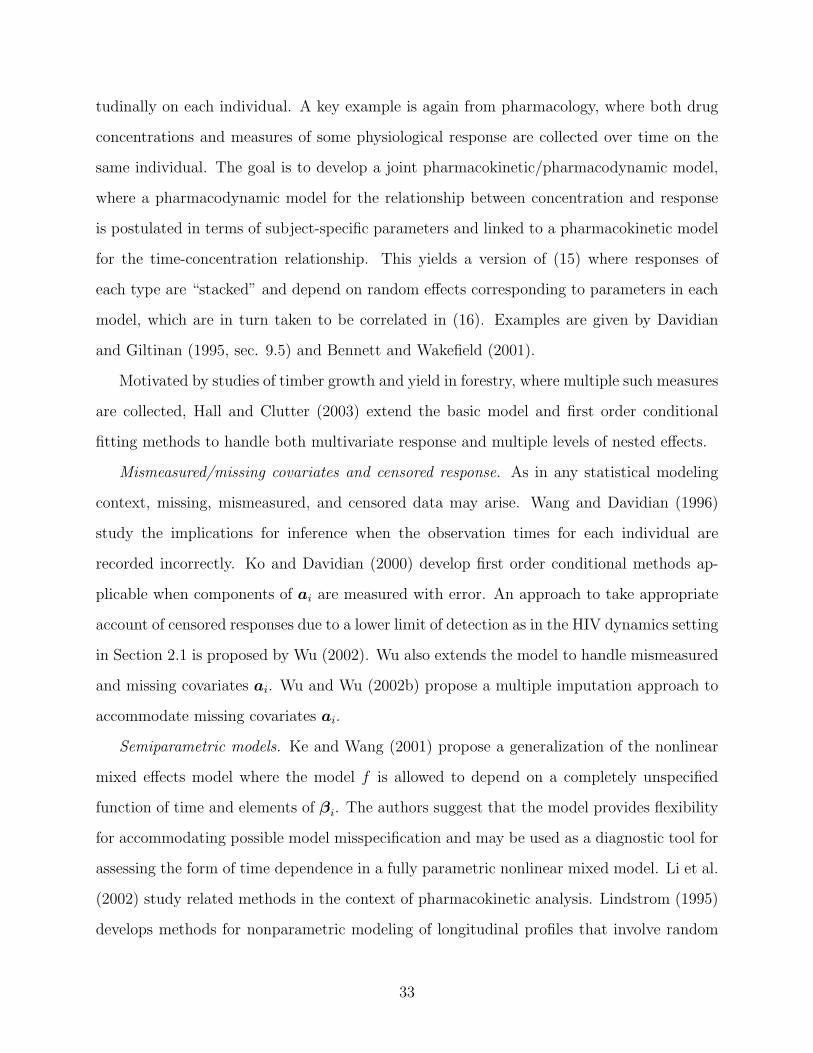
tudinally on each individual. A key example is again from pharmacology, where both drug
concentrations and measures of some physiological response are collected over time on the
same individual. The goal is to develop a joint pharmacokinetic/pharmacodynamic model,
where a pharmacodynamic model for the relationship between concentration and response
is postulated in terms of subject-specific parameters and linked to a pharmacokinetic model
for the time-concentration relationship. This yields a version of (15) where responses of
each type are “stacked” and depend on random effects corresponding to parameters in each
model, which are in turn taken to be correlated in (16). Examples are given by Davidian
and Giltinan (1995, sec. 9.5) and Bennett and Wakefield (2001).
Motivated by studies of timber growth and yield in forestry, where multiple such measures
are collected, Hall and Clutter (2003) extend the basic model and first order conditional
fitting methods to handle both multivariate response and multiple levels of nested effects.
Mismeasured/missing covariates and censored response. As in any statistical modeling
context, missing, mismeasured, and censored data may arise. Wang and Davidian (1996)
study the implications for inference when the observation times for each individual are
recorded incorrectly. Ko and Davidian (2000) develop first order conditional methods ap-
plicable when components of ai are measured with error. An approach to take appropriate
account of censored responses due to a lower limit of detection as in the HIV dynamics setting
in Section 2.1 is proposed by Wu (2002). Wu also extends the model to handle mismeasured
and missing covariates ai. Wu and Wu (2002b) propose a multiple imputation approach to
accommodate missing covariates ai.
Semiparametric models. Ke and Wang (2001) propose a generalization of the nonlinear
mixed effects model where the model f is allowed to depend on a completely unspecified
function of time and elements of βi. The authors suggest that the model provides flexibility
for accommodating possible model misspecification and may be used as a diagnostic tool for
assessing the form of time dependence in a fully parametric nonlinear mixed model. Li et al.
(2002) study related methods in the context of pharmacokinetic analysis. Lindstrom (1995)
develops methods for nonparametric modeling of longitudinal profiles that involve random
33
effects and may be fitted using standard nonlinear mixed model techniques.
Other topics. Methods for model selection and determination are studied by Vonesh,
Chinchilli, and Pu (1996), Dey, Chen, and Chang (1997), and Wu and Wu (2002a). Young,
Zerbe, and Hay (1997) propose confidence intervals for ratios of components of the fixed
effects β. Oberg and Davidian (2000) propose methods for estimating a parametric transfor-
mation of the response under which the Stage 1 conditional density is normal with constant
variance. Concordet and Nunez (2000) and Chu et al. (2001) discuss interesting applications
in veterinary science involving calibration and prediction problems. Methods for combining
data from several studies where each is represented by a nonlinear mixed model are dis-
cussed by Wakefield and Rahman (2000) and Lopes, Muller, and Rosner (2003). Yeap and
Davidian (2001) propose “robust” methods for accommodating “outlying” responses within
individual or “outlying” individuals. Lai and Shih (2003) develop alternative methods to
those of Mentre and Mallet (1994) cited in Section 3.4 that do not require consideration of
the joint distribution of βi and ai. For a model of the form (16), the distribution of the bi
is left completely unspecified and is estimated nonparametrically; these authors also derive
large-sample properties of the approach.
Pharmaceutical applications. A topic that has generated great recent interest in the phar-
maceutical industry is so-called “clinical trial simulation.” Here, a hypothetical population
is simulated to which the analyst may apply different drug regimens according to different
designs to evaluate potential study outcomes. Nonlinear mixed models are at the heart of
this enterprise; subjects are simulated from mixed models for pharmacokinetic and pharma-
codynamic behavior that incorporate variation due to covariates and “unexplained” sources
thought to be present. See, for example, http://www.pharsight.com/products/trial simulator.
More generally, nonlinear mixed effects modeling techniques have been advocated for popula-
tion pharmacokinetic analysis in a guidance issued by the U.S. Food and Drug Administration
(http://www.fda.gov/cder/guidance/1852fnl.pdf).
5. DISCUSSION
This review of nonlinear mixed effects modeling is of necessity incomplete, as it is beyond
34

the limits of a single article to document fully the extensive literature. We have chosen to
focus much of our attention on revisiting the considerations underlying the basic model from
an updated standpoint, and we hope that this will offer readers familiar with the topic addi-
tional insight and provide those new to the model a foundation for appreciating its rationale
and utility. We have not presented an analysis of a specific application; the references cited
in Section 2.1 and Clayton et al. (2003) and Yeap et al. (2003) in this issue offer detailed
demonstrations of the formulation, implementation, and interpretation of nonlinear mixed
models in practice. We look forward to continuing methodological developments for and new
applications of this rich class of models in the statistical and subject-matter literature.
ACKNOWLEDGMENTS
This research was partially supported by NIH grants R01-CA085848 and R37-AI031789.
REFERENCES
Beal, S.L., and Sheiner, L.B. (1982), “Estimating Population Pharmacokinetics,” CRC CriticalReviews in Biomedical Engineering, 8, 195–222.
Bennett, J., and Wakefield, J. (2001), “Errors-in-Variables in Joint Population Pharmacokinet-ic/Pharmacodynamic Modeling,” Biometrics, 57, 803–812.
Boeckmann, A.J., Sheiner, L.B., and Beal S.L. (1992), NONMEM User’s Guide, Part V, Intro-ductory Guide, San Francisco: University of California.
Breslow, N.E., and Clayton, D.G. (1993), “Approximate Inference in Generalized Linear MixedModels,” Journal of the American Statistical Association, 88, 9–25.
Carlin, B.P., and Louis, T.A. (2000), Bayes and Empirical Bayes Methods for Data Analysis,Second Edition, New York: Chapman and Hall/CRC Press.
Chu, K.K., Wang, N.Y., Stanley, S., and Cohen, N.D. (2001), “Statistical Evaluation of the Reg-ulatory Guidelines for Use of Furosemide in Race Horses,” Biometrics, 57, 294–301.
Clarkson, D.B., and Zhan, Y.H. (2002), “Using Spherical-Radial Quadrature to Fit GeneralizedLinear Mixed Effects Models,” Journal of Computational and Graphical Statistics, 11, 639–659.
Clayton, C.A., T.B. Starr, R.L. Sielken, Jr., R.L. Williams, P.G. Pontal, A.J. Tobia. (2003), ‘Usinga Non-linear Mixed Effects Model to Characterize Cholinesterase Activity in Rats Exposed toAldicarb,” Journal of Agricultural, Biological, and Environmental Statistics, 8, ????-????.
Concordet, D., and Nunez, O.G. (2000), “Calibration for Nonlinear Mixed Effects Models: AnApplication to the Withdrawal Time Prediction,” Biometrics, 56, 1040–1046.
Davidian, M., and Gallant, A. R. (1992a). Nlmix: A program for maximum likelihood estimationof the nonlinear mixed effects model with a smooth random effects density. Department ofStatistics, North Carolina State University.
Davidian, M., and Gallant, A.R. (1992b), “Smooth Nonparametric Maximum Likelihood Estima-tion for Population Pharmacokinetics, With Application to Quinidine,” Journal of Pharmacoki-netics and Biopharmaceutics, 20, 529–556.
35

Davidian, M., and Gallant, A.R. (1993), “The Nonlinear Mixed Effects Model With a SmoothRandom Effects Density,” Biometrika, 80, 475–488.
Davidian, M., and Giltinan, D.M. (1993), “Some simple methods for estimating intra-individualvariability in nonlinear mixed effects models,” Biometrics, 49, 59–73.
Davidian, M., and Giltinan, D.M. (1995), Nonlinear Models for Repeated Measurement Data, NewYork: Chapman and Hall.
Demidenko, E. (1997), “Asymptotic Properties of Nonlinear Mixed Effects Models,” in ModelingLongitudinal and Spatially Correlated Data: Methods, Applications, and Future Directions, eds.,T.G. Gregoire, D.R., Brillinger, P.J. Diggle, E. Russek-Cohen, W.G. Warren, and R.D. Wolfinger,New York: Springer.
Dey, D.K., Chen, M.H., and Chang, H. (1997), “Bayesian Approach for Nonlinear Random EffectsModels,” Biometrics, 53, 1239–1252.
Diggle, P.J., Heagerty, P., Liang, K.-Y., and Zeger, S.L. (2001), Analysis of Longitudinal Data,Second Edition, Oxford: Oxford University Press.
Hall, D.B., and Bailey, R.L. (2001), “Modeling and Prediction of Forest Growth Variables Basedon Multilevel Nonlinear Mixed Models,” Forest Science, 47, 311–321.
Hall, D.B., and Clutter, M. (2003), “Multivariate multilevel nonlinear mixed effects models fortimber yield predictions. ” Biometrics, in press.
Hartford, A., and Davidian, M. (2000), “Consequences of Misspecifying Assumptions in NonlinearMixed Effects Models,” Computational Statistics and Data Analysis, 34, 139–164.
Heagerty, P. (1999), “Marginally Specified Logistic-Normal Models for Longitudinal Binary Data,”Biometrics, 55, 688–698.
Fang, Z. and Bailey, R.L. (2001), “Nonlinear Mixed Effects Modeling for Slash Pine DominantHeight Growth Following Intensive Silvicultural Treatments,” Forest Science, 47, 287–300.
Galecki, A.T. (1998), “NLMEM: A New SAS/IML Macro for Hierarchical Nonlinear Models,”Computer Methods and Programs in Biomedicine, 55, 207–216.
Gelman, A., Bois, F., and Jiang, L.M. (1996), “Physiological Pharmacokinetic Analysis UsingPopulation Modeling and Informative Prior Distributions,”Journal of the American StatisticalAssociation, 91, 1400–1412.
Gregoire, T.G., and Schabenberger, O. (1996a), “Nonlinear Mixed-Effects Modeling of CumulativeBole Volume With Spatially-Correlated Within-Tree Data,” Journal of Agricultural, Biological,and Environmental Statistics, 1, 107–119.
Gregoire, T.G., and Schabenberger, O. (1996b), “A Non-Linear Mixed-Effects Model to PredictCumulative Bole Volume of Standing Trees,” Journal of Applied Statistics, 23, 257–271.
Karlsson, M.O., Beal, S.L., and Sheiner, L.B. (1995), “Three New Residual Error Models forPopulation PK/PD Analyses,” Journal of Pharmacokinetics and Biopharmaceutics, 23, 651–672.
Karlsson, M.O., and Sheiner, L.B. (1993), “The Importance of Modeling Inter-Occasion Variabilityin Population Pharmacokinetic Analyses,” Journal of Pharmacokinetics and Biopharmaceutics,21, 735–750.
Ke, C. and Wang, Y. (2001), “Semiparametric Nonlinear Mixed Models and Their Applications,”Journal of the American Statistical Association, 96, 1272–1298.
Ko, H.J., and Davidian, M. (2000), “Correcting for Measurement Error in Individual-Level Co-variates in Nonlinear Mixed Effects Models,” Biometrics, 56, 368–375.
Lai, T.L., and Shih, M.-C. (2003), “Nonparametric Estimation in Nonlinear Mixed Effects Models,”Biometrika, 90, 1–13.
36

Law, N.J., Taylor, J.M.G., and Sandler, H. (2002), “The Joint Modeling of a Longitudinal DiseaseProgression Marker and the Failure Time Process in the Presence of a Cure,” Biostatistics, 3,547–563.
Li, L., Brown, M.B., Lee, K.H., and Gupta, S. (2002), “Estimation and Inference for a Spline-Enhanced Population Pharmacokinetic Model,” Biometrics, 58, 601–611.
Lindstrom, M.J. (1995), “Self-Modeling With Random Shift and Scale Parameters and a Free-KnotSpline Shape Function,” Statistics in Medicine, 14, 2009–2021.
Lindstrom, M.J., and Bates, D.M. (1990), “Nonlinear Mixed Effects Models for Repeated MeasuresData,” Biometrics, 46, 673–687.
Littell, R.C., Milliken, G.A., Stroup, W.W., and Wolfinger, R.D. (1996), SAS System for MixedModels, Cary NC: SAS Institute Inc.
Lopes, H.F., Muller, P., and Rosner, G.L. (2003), “Bayesian meta-analysis for longitudinal datamodels using multivariate mixture priors, Biometrics, 59, 66–75.
Mallet, A. (1986), “A Maximum Likelihood Estimation Method for Random Coefficient RegressionModels,” Biometrika, 73, 645–656.
Mandema, J.W., Verotta, D., and Sheiner, L.B., (1992), “Building Population Pharmacokinetic/Phar-macodynamic Models,” Journal of Pharmacokinetics and Biopharmaceutics, 20, 511–529.
McRoberts, R.E., Brooks, R.T., and Rogers, L.L. (1998), “Using Nonlinear Mixed Effects Modelsto Estimate Size-Age Relationships for Black Bears,” Canadian Journal of Zoology, 76, 1098–1106.
Mentre, F., and Mallet, A. (1994), “Handling Covariates in Population Pharmacokinetics,” Inter-national Journal of Biomedical Computing, 36, 25–33.
Mezzetti, M., Ibrahim, J,.G., Bois, F.Y., Ryan, L.M., Ngo, L., and Smith, T.J. (2003), “A BayesianCompartmental Model for the Evaluation of 1,3-Butadiene Metabolism,” Applied Statistics, 52,291–305.
Mikulich, S.K., Zerbe, G.O., Jones, R.H., and Crowley, T.J. (2003), “Comparing Linear andNonlinear Mixed Model Approaches to Cosinor Analysis,” Statistics in Medicine, 22, 3195–3211.
Monahan, J., and Genz, A. (1997), “Spherical-Radial Integration Rules for Bayesian Computa-tion,” Journal of the American Statistical Association, 92, 664–674.
Morrell, C.H., Pearson, J.D., Carter, H.B., and Brant, L.J. (1995), “Estimating Unknown Tran-sition Times Using a Piecewise Nonlinear Mixed-Effects Model in Men With Prostate Cancer,”Journal of the American Statistical Association, 90, 45–53.
Muller, P., and Rosner, G.L. (1997), “A Bayesian Population Model With Hierarchical MixturePriors Applied to Blood Count Data,” Journal of the American Statistical Association, 92, 1279–1292.
Notermans, D.W., Goudsmit, J., Danner, S.A., de Wolf, F., Perelson, A.S., and Mittler, J. (1998).Rate of HIV-1 decline following antiretroviral therapy is related to viral load at baseline and drugregimen. AIDS 12, 1483–1490.
Oberg, A., and Davidian, M. (2000), “Estimating Data Transformations in Nonlinear Mixed EffectsModels,” Biometrics, 56, 65–72.
Pauler, D. and Finkelstein, D. (2002), “Predicting Time to Prostate Cancer Recurrence Based onJoint Models for Non-linear Longitudinal Biomarkers and Event Time,” Statistics in Medicine,21, 3897–3911.
Pilling, G.M., Kirkwood, G.P., and Walker, S.G. (2002), “An Improved Method for EstimatingIndividual Growth Variability in Fish, and the Correlation Between von Bertalanffy GrowthParameters,” Canadian Journal of Fisheries and Aquatic Sciences, 59, 424–432.
37
Pinheiro, J.C., and Bates, D.M. (1995), “Approximations to the Log-Likelihood Function in theNonlinear Mixed-Effects Model,” Journal of Computational and Graphical Statistics, 4, 12–35.
Pinheiro, J.C., and Bates, D.M. (2000), Mixed-Effects Models in S and Splus, New York: Springer.SAS Institute (1999), PROC NLMIXED, SAS OnlineDoc, Version 8, Cary, NC: SAS InstituteInc.
Schumitzky, A. (1991), “Nonparametric EM Algorithms for Estimating Prior Distributions,” Ap-plied Mathematics and Computation, 45, 143–157
Steimer, J.L., Mallet, A., Golmard, J.L., and Boisvieux, J.F. (1984), “Alternative Approaches toEstimation of Population Pharmacokinetic Parameters: Comparison with the Nonlinear MixedEffect Model,” Drug Metabolism Reviews, 15, 265–292.
Raudenbush, S.W., Yang, M.L., and Yosef, M. (2000), “Maximum Likelihood for Generalized Lin-ear Models With Nested Random Effects Via High-Order, Multivariate Laplace Approximation,”Journal of Computational and Graphical Statistics, 9, 141–157.
Rekaya, R., Weigel, K.A., and Gianola, D. (2001), “Hierarchical Nonlinear Model for Persistency ofMilk Yield in the First Three Lactations of Holsteins,” Lifestock Production Science, 68, 181–187.
Rodriguez-Zas, S.L., Gianola, D., and Shook, G.E. (2000), “Evaluation of models for somatic cellscore lactation patterns in Holsteins,” Lifestock Production Science, 67, 19–30.
Rosner, G.L, and Muller, P. (1994), “Pharmacokinetic/Pharmacodynamic Analysis of HematologicProfiles,” Journal of of Pharmacokinetics and Biopharmaceutics, 22, 499–524.
Schabenberger, O., and Pierce, F.J. (2002), Contemporary Statistical Models for the Plant and SoilSciences, New York: CRC Press.
Sheiner, L.B., and Ludden, T.M. (1992), “Population pharmacokinetics/pharmacodynamics,” An-nual Review of Pharmacological Toxicology, 32, 185–209.
Sheiner, L.B., Rosenberg, B., and Marathe, V.V. (1977), “Estimation of Population Characteristicsof Population Pharmacokinetic Parameters From Routine Clinical Data,” Journal of Pharma-cokinetics and Biopharmaceutics, 8, 635–651.
Verbeke, G., and Molenberghs, G. (2000), Linear Mixed Models for Longitudinal Data, New York:Springer.
Vonesh, E.F. (1996), “A Note on the Use of Laplace’s Approximation for Nonlinear Mixed-EffectsModels,” Biometrika, 83, 447–452.
Vonesh, E.F. (1992), “Mixed-Effects Nonlinear Regression for Unbalanced Repeated Measures,”Biometrics, 48, 1–17.
Vonesh, E.F., and Chinchilli, V.M. (1997), Linear and Nonlinear Models for the Analysis of Re-peated Measurements, New York: Marcel Dekker.
Vonesh, E.F., Chinchilli, V.M., and Pu, K.W. (1996), “Goodness-Of-Fit in Generalized NonlinearMixed-Effects Models,” Biometrics, 52, 572–587.
Vonesh, E.G., Wang, H., Nie, L., and Majumdar, D. (2002), “Conditional Second-Order General-ized Estimating Equations for Generalized Linear and Nonlinear Mixed-Effects Models,” Journalof the American Statistical Association, 97, 271–283.
Wakefield, J. (1996), “The Bayesian Analysis of Population Pharmacokinetic Models,” Journal ofthe American Statistical Association, 91, 62–75.
Wakefield, J. and Rahman, N. (2000), “The Combination of Population Pharmacokinetic Studies,”Biometrics, 56, 263–270.
Wakefield, J.C., Smith, A.F.M., Racine-Poon, A., and Gelfand, A.E. (1994), “Bayesian Analysisof Linear and Nonlinear Population Models by Using the Gibbs Sampler,” Applied Statistics, 43,201–221.
38

Walker, S.G. (1996), “An EM algorithm for Nonlinear Random Effects Models,” Biometrics, 52.934–944.
Wang, N., and Davidian, M. (1996), “A Note on Covariate Measurement Error in Nonlinear MixedEffects Models,” Biometrika, 83, 801–812.
Wolfinger, R. (1993), “Laplace’s Approximation for Nonlinear Mixed Models,” Biometrika, 80,791–795.
Wolfinger, R.D., and Lin, X. (1997), “Two Taylor-series Approximation Methods for NonlinearMixed Models,” Computational Statistics and Data Analysis, 25, 465–490.
Wu, H.L., and Ding, A.A. (1999), “Population HIV-1 Dynamics in vivo: Applicable Models andInferential Tools for Virological Data From AIDS Clinical Trials,” Biometrics, 55, 410–418.
Wu, H.L., and Wu, L. (2002a), “Identification of Significant Host Factors for HIV DynamicsModelled by Non-Linear Mixed-Effects Models,” Statistics in Medicine, 21, 753–771.
Wu, L. (2002), “A Joint Model for Nonlinear Mixed-Effects Models With Censoring and CovariatesMeasured With Error, With Application to AIDS Studies,” Journal of the American StatisticalAssociation, 97, 955–964.
Wu, L., and Wu, H.L. (2002b), “Missing Time-Dependent Covariates in Human ImmunodeficiencyVirus Dynamic Models,” Applied Statistics, 51, 2002.
Yeap, B.Y., Catalano, P.J., Ryan, L.M., and Davidian, M. (2003), ‘Robust Two-Stage Approach toRepeated Measurements Analysis of Chronic Ozone Exposure in Rats,” Journal of Agricultural,Biological, and Environmental Statistics, 8, ????-????.
Yeap, B.Y., and Davidian, M. (2001), “Robust Two-Stage Estimation in Hierarchical NonlinearModels,” Biometrics, 57, 266–272.
Young, D.A., Zerbe, G.O., and Hay, W.W. (1997), “Fieller’s Theorem, Scheff’e SimultaneousConfidence Intervals, and Ratios of Parameters of Linear and Nonlinear Mixed-Effects Models,”Biometrics, 53, 838–347.
Zeng, Q., and Davidian, M. (1997), “Testing Homgeneity of Intra-run Variance Parameters inImmunoassay,” Statistics in Medicine, 16, 1765–1776.
39
Time (hr)
The
ophy
lline
Con
c. (
mg/
L)
0 5 10 15 20 25
02
46
810
12
Figure 1. Theophylline concentrations for 12 subjects following a single oral dose.
40

0 20 40 60 80
12
34
56
7
Days
log1
0 P
lasm
a R
NA
(co
pies
/ml)
Figure 2. Viral load profiles for 10 subjects from the ACTG 315 study. The lower limit of
detection of 100 copies/ml is denoted by the dotted line.
41

0 5 10 15 20
02
46
810
12
y
t
Figure 3. Intra-individual sources of variation. The solid line is the “inherent” trajectory, the
dotted line is the “realization” of the response process that actually takes place, and the solid
diamonds are measurements of the “realization” at particular time points that are subject to
error.
42
Related Documents