Nonlinear Fiber Optics for Bio-Imaging by Roque Gagliano Molla Ingeniero Electricista Universidad de la República, Montevideo, Uruguay, 2001 Submitted to the Department of Electrical Engineering and Computer Science and the faculty of the Graduate School of the University of Kansas in partial fulfillment of the requirements for the degree of Master of Science. Chair: Dr. Rongqing Hui Dr. Victor Frost Dr. Kenneth Demarest Date of Thesis Defense: May 20 th , 2005

Welcome message from author
This document is posted to help you gain knowledge. Please leave a comment to let me know what you think about it! Share it to your friends and learn new things together.
Transcript

Nonlinear Fiber Optics for Bio-Imaging
by
Roque Gagliano Molla
Ingeniero Electricista
Universidad de la República, Montevideo, Uruguay, 2001
Submitted to the Department of Electrical Engineering and Computer Science and the
faculty of the Graduate School of the University of Kansas in partial fulfillment of the
requirements for the degree of Master of Science.
Chair: Dr. Rongqing Hui
Dr. Victor Frost
Dr. Kenneth Demarest
Date of Thesis Defense: May 20th, 2005

Acknowledgements I would like to show my appreciation and gratitude to my advisor Dr. Rongqing Hui.
This has been an amusing and rewarding learning experience that we started by
putting some living cells in a Pyrex back in January 2004. I would like to thank him
not only for his advice and financial support but also for being an endless source of
optimism and an example of self-motivation.
I would also like to thank the rest of my committee, Dr. Victor Frost and Dr. Kenneth
Demarest.
Special thanks to Jay Unruh and the rest of the group at Dr. Carey Johnson’s
laboratory of the Chemistry Department at the University of Kansas where all the
experiments of this work were performed.
Also, I would like to acknowledge the Fulbright Program, the OAS-LASPAU
Program, the Barca Family and the KU International Program for their support.
Finally I would like to thank my family and friend for helping me removing all the
obstacles in order to make my dream of a graduate education possible.
ii

Table of Contents Acknowledgements........................................................................................................... ii
Table of Contents.............................................................................................................iii
List of Figures ..................................................................................................................vi
Abstract ..........................................................................................................................viii
Chapter 1: Introduction............................................................................................... 1
1.1 Motivation......................................................................................................... 1
1.2 Two-photon microscopy and wavelength-tunable pulsed laser sources........... 1
1.3 Organization...................................................................................................... 4
Chapter 2: Nonlinear Effects of Optical Fibers .......................................................... 5
2.1 General Analysis............................................................................................... 5
2.2 Nonlinear Pulse Propagation............................................................................. 7
2.3 Chromatic Dispersion ..................................................................................... 10
2.4 Nonlinear effects............................................................................................. 11
2.4.1 Self Phase Modulation (SPM) ................................................................ 11
2.4.2 Cross Phase Modulation (XPM) ............................................................. 12
2.4.3 Four Wave Mixing (FWM)..................................................................... 12
2.4.4 Stimulated Raman Scattering (SRS)....................................................... 13
2.4.5 Stimulated Brillouin Scattering (SBS).................................................... 15
2.5 Split Step Fourier Method............................................................................... 15
Chapter 3: Optical Solitons....................................................................................... 17
3.1 Solitons in Physics .......................................................................................... 17
3.2 Fiber Solitons .................................................................................................. 18
3.3 Fundamental Soliton ....................................................................................... 20
3.4 Higher Order Solitons ..................................................................................... 20
3.5 Soliton Interaction........................................................................................... 20
3.6 Loss-Managed Solitons................................................................................... 21
3.7 Dispersion Management Solitons (Average Solitons).................................... 22
Chapter 4: Short Pulsed Fiber Lasers ....................................................................... 24
iii

4.1 Short Pulsed Cavity Lasers ............................................................................. 24
4.2 Mode-locking.................................................................................................. 25
4.2.1 Active Mode-locking .............................................................................. 26
4.2.2 Passive Mode Locking............................................................................ 26
4.3 Solid State Laser ............................................................................................. 27
4.4 Fiber Lasers..................................................................................................... 29
4.4.1 Ring Cavity Fiber Lasers ........................................................................ 30
4.4.2 Fabry-Perot or Linear cavities ................................................................ 32
4.5 High Power Pulsed Fiber Lasers..................................................................... 33
Chapter 5: Photonic Crystal Fibers........................................................................... 35
5.1 Fundamentals of photonic crystal waveguiding ............................................. 35
5.2 Classification of PCF ...................................................................................... 36
5.3 Modelling of microstructured fibers ............................................................... 37
5.4 Fabrication of photonic crystal fibers ............................................................. 39
5.5 Applications .................................................................................................... 40
Chapter 6: Experimental and Numerical Analysis of Soliton Self-Frequency Shift 42
6.1 Experimental Results ...................................................................................... 42
6.2 Generalized Non-Linear Schrödinger Equation.............................................. 45
6.3 Numerical Analysis......................................................................................... 49
Chapter 7: Analytical Analysis of Soliton Self-Frequency Shift.............................. 60
7.1 Analytical Model ............................................................................................ 61
7.2 Limitations of the previous analytical model.................................................. 66
7.3 A semi-analytical method for soliton self frequency shift in an optical fiber.67
7.3.1 Semi-Analytic Method Formulation ....................................................... 68
7.3.2 Results and Discussion. .......................................................................... 72
Chapter 8: Short Pulsed Lasers Applications for Two Photons Microscopy ........... 79
8.1 One-Photon Confocal Microscopy ................................................................. 80
8.2 Two Photons Microscopy ............................................................................... 82
8.3 Experimental Acquisition of Two-Photon Microscopy.................................. 84
iv

8.4 Other applications ........................................................................................... 89
CONCLUSIONS............................................................................................................. 90
FUTURE WORK............................................................................................................ 92
GLOSSARY ................................................................................................................... 93
REFERENCES ............................................................................................................... 95
APPENDIX A: Optical Fibers Characteristics ............................................................... 99
APPENDIX B: VPI Models and Numerical Parameters .............................................. 104
APPENDIX B: MATLAB CODE ................................................................................ 116
APPENDIX D: Submitted Publication ......................................................................... 118
v

List of Figures Figure 2.1: Stimulated Raman Scattering. ..................................................................... 14
Figure 4.1: Ti:Sapphire laser setup with Argon CW pump and self-mode-locking. ...... 28
Figure 4.2 All-fiber ring-laser. ....................................................................................... 31
Figure 4.3 Pulses Shortening in a Ring Fiber Laser [Nel97]. ....................................... 31
Figure 4.4: Schematic of a fiber laser ............................................................................ 33
Figure 4.5: MM fiber oscillator side-pumped ................................................................ 34
Figure 5.1: Classification of PCF [Bja03]..................................................................... 36
Figure 5.2: Geometrical characteristics of PCF. ........................................................... 37
Figure 6.1: Experimental Setup for a Wavelength-Tunable Pulsed Laser Source......... 43
Figure 6.2: Experimental spectrums for a wavelength shifter ....................................... 44
Figure 6.3: Raman Response Function [Agr01]. ........................................................... 46
Figure 6.3: Normalized Raman Gain for a SiO2 fiber. .................................................. 47
Figure 6.5: Soliton formation from the original pump pulse.......................................... 50
Figure 6.6: Time domain Characteristics of the output from a 7m HNL-PCF. ............. 51
Figure 6.7: Wavelength Shift for different Input Average Power in a 7m HNL-PCF. ... 52
Figure 6.8: Wavelength Shift and Input Average Power for 3m and 7m HNL-PCF...... 54
Figure 6.9: Supercontinuum generation after applying 5mW pulses to 7m of PCF. ..... 55
Figure 6.10: Time domain characteristics for different HNL-PCF lengths ................... 56
Figure 6.11: Wavelength Shift and Fiber length for a HNL-PCF. ................................. 57
Figure 6.12: Soliton Pulse width and Fiber Length for a HNL-PCF. ............................ 58
Figure 6.13: Soliton order N ans fiber length. ............................................................... 59
Figure 6.14: Numerical and Experimental Results Wavelength Shifts........................... 59
Figure 7.1: Semi-analytical method for SSFS in an optical fiber. ................................. 68
Figure 7.2: Block diagram for the semi-analytical method............................................ 72
Figure 7.3: Frequency shift versus pulse width for a 100m PMF. ................................. 74
Figure 7.4: SSFS for a HNL-PCF with different fiber lengths in log scale.................... 75
Figure 7.5: Frequency shift and pulse width for a 10m HNL-PCF............................... 76
vi

Figure 7.6: Wavelength shift and fiber length for a PCF.............................................. 77
Figure 8.1: A Scanning Laser Confocal Microscope Setup. .......................................... 80
Figure 8.2: Absorption and emission spectrum of the Alexa-series dyes. ...................... 82
Figure 8.3: Experimental setup for acquiring a two-photon image. .............................. 86
Figure 8.4: Two-photon image of a fluosphere using a 780nm pump laser................... 87
Figure 8.5: Radial intensity profile for a fluosphere using a pump laser at 780nm. ..... 87
Figure 8.6: Two-photon image of a fluosphere using a shifted pump laser to 920nm. .. 88
Figure 8.7: Radial intensity profile for the fluosphere at the center of figure 8.6. ........ 88
Figure A.1: Crystal Fibre NL-18-710 axial profile (http://www.crystal-fibre.com) ..... 99
Figure A.2: Attenuation Parameter (α) for Crystal Fibre NL-18-710. ........................ 101
Figure A.3: Nonlinear Coefficient (γ) for a Crystal Fibre NL-18-710. ........................ 101
Figure A.4: Dispersion Coefficient (D) for a Crystal Fibre NL-18-710. ..................... 102
Figure B.1: VPI Model used for simulations. ............................................................... 104
vii

Abstract Two-photon excitation (TPE) is a modern technology with applications in microscopy
and spectroscopy that has gained a great amount of attention in recent years. This
technique is the best suitable to analyze thick tissues and live animals as it works in
the near-infrared (NIR) region.
In this work we implement and evaluate a two-photon setup that allows the shifting of
the working wavelength over a wide range using the soliton self-frequency shift
(SSFS) effect. The shifter is implemented using a pulsed fiber laser and a photonic
crystal fiber (PCF). We also include a numerical evaluation of the dependency of the
fiber shift on the input average power and the fiber length.
A semi-analytical model is proposed to investigate the characteristics of the SSFS in
optical fibers. SSFS in two different types of fibers were evaluated and the results
agree very well with those of numerical simulations. We show that when the
frequency shift is small enough, it is inversely proportional to the fourth power of the
initial soliton pulse width. However, with large frequency shift, this fourth power rule
needs to be modified.
We finally show the first two-photon images obtained at the University of Kansas.
viii

Chapter 1: Introduction
1.1 Motivation Every day one is bombarded with press releases covering new discoveries in areas
such as DNA analysis and molecular analysis. Many of these new technological
breakthroughs are achieved thanks to the use of powerful microscopy instruments that
rely heavily on lasers [Sch01]. In this work we investigate innovative technologies
that open the doors for the improvement of existing instruments as well as of our
understanding of these phenomena.
1.2 Two-photon microscopy and wavelength-tunable pulsed laser sources
When using florescence microscopy, the pump’s photons are absorbed by the target
substance which then emits a photon in a longer wavelength. Different species are
labeled with different fluorescent dyes that emit in different wavelengths.
Recognizing a dye is equivalent to recognizing the targeted molecule.
A particular technique that has growing interest in the scientific community is the
two-photon laser scanning microscopy (TPLSM), where two photons from the pump
are absorbed simultaneously to generate one signal photon. This techniques allows
higher penetration lengths (you can see deeper into the object) and higher resolution
1

(you can see smaller objects) than conventional confocal microscopy instruments
[Den90].
A classical fluorescence microscopy instrument includes a solid state pulsed laser.
These devices are not only expensive, but also difficult to manipulate and not suitable
for field operation. In recent years, all-fiber pulsed laser based in fiber amplifiers have
become commercially available. These lasers are compact, easy to operate and easy to
translate. Their output power has consistently increased during the past two years
[Nel97].
In a photonic crystal fiber (PCF), air-holes are located around the core [Bja03]. These
air structures have several designs for different applications. A very common
implementation is characterized by its very high nonlinear index. Thanks to this high
non-linear parameter and due to the stimulated Raman scattering (SRS), as high-
power short pulses propagate along the fiber, an optical soliton is formed. The
soliton’s central frequency is then shifted to lower values [Nor02].
Fundamental optical solitons are pulses that do not change their shape while
propagating along an optical fiber [Agr03]. Raman solitons are formed from the
breaking of a high power pulse and have the characteristic of shifting their frequency
as a function of their pulse width [Bea87]. The soliton self-frequency shift (SSFS)
was first discovered by Mitschke et al in 1986 [Mit86]. At the same time, Gordon
2

[Gor86] formulated how the frequency shift inversely depends on the fourth power of
its width. However, this formulation does not take into account the fiber losses and
the frequency dependency of the fiber parameters. As the pulse changes its central
wavelength, the fiber group-delay dispersion, nonlinear parameter, effective area and
attenuation can vary considerably, modifying the fourth power rule [Gor86].
In this work we introduce a simple semi-analytic method to model SSFS in optical
fibers. By taking into account the fiber wavelength dependent attenuation, dispersion
and nonlinearity, we show that the SSFS becomes less sensitive to the input pulse
width when this width is narrow enough and the fourth power rule needs to be
modified for many practical applications. The results of semi-analytic calculations are
found to be in good agreement with numerical simulations using the split-step Fourier
method. Our results also indicate that the fourth-power rule predicted in [Gor86] is
accurate when the wavelength shift is small and the fiber loss is negligible.
Thanks to the SSFS, we were able to implement a highly wavelength-tunable pulsed
fiber laser that delivers femtosecond pulses to a two-photon microscope. The
wavelength tunable capability was achieved by introducing a PCF in the light path.
The two-photon images shown in this work were the first ones performed at the
University of Kansas [Nor02].
3

1.3 Organization
This Thesis is organized as follows: Chapters 2 to 5 introduce concepts such as
nonlinear effects in optical fibers, optical solitons, short pulses fiber lasers and
photonic crystal fibers. This work also includes extensive references for further study
of these topics.
In Chapter 6 we study the propagation of a short pulse in an optical fiber, particularly
in a PCF. We show numerical results for different input powers and fiber lengths and
contrast some of these simulations with experimental data.
A detailed analysis of the SSFS phenomenon is done in Chapter 7, where the semi-
analytical method is introduced. The results are also contrasted with numerical data
and with the analytical model in [Gor86].
In the last chapter we briefly describe a two-photon microscopy system and we show
the recorded images. These experiments were performed at Dr. Carey Johnson’s
laboratory at the Department of Chemistry of the University of Kansas.
Finally we present our conclusions and describe possible future works.
4

Chapter 2: Nonlinear Effects of Optical Fibers
2.1 General Analysis
The propagation of an electromagnetic field along an optical fiber is generically
described by Maxwell´s Equations [Agr01] from which we deduce the wave equation:
( ) ( ) ( )2
2
02
2 ,,1,t
trPt
trEc
trE∂
∂−
∂∂
−=×∇×∇rrrr
rr µ (2.1.1)
Where Er
is the electrical field, Pr
the induced polarization, ε0 is the vacuum
permittivity, µ0 the vacuum permeability and 00
1εµ
=c is the speed of the light in
vacuum. Although the relationship between Er
and Pr
will normally require a
quantum-mechanical study, many times a phenomenological relationship can be
applied:
( ) ( ) ( )( )Krrr
Mrrrr
+++= EEEEEEP 3210 : χχχε (2.1.2)
Where χ(j) is the jth order susceptibility, generally a tensor of rank j+1. The term j=1
represents the linear relationship; it affects the refractive index and the attenuation
coefficient of the fiber. The second order susceptibility, responsible for second order
harmonic generation, is negligible for SiO2 and thus is not present in optical fibers.
The third order susceptibility, χ(3), is responsible for phenomena such as third order
5

harmonic generation, four-wave mixing and nonlinear refraction (Kerr effect). In this
last effect, the intensity dependency of the refractive index is reflected as:
( ) 2
2
2,~ EnnEn
rr+=⎟
⎠⎞⎜
⎝⎛ ωω (2.1.3)
Where n(ω) represent the linear contribution and n2 is the nonlinear-index, related to
χ(3).
If we include the nonlinear effects, the induced polarization is obtained by adding two
terms: the linear contribution ( )( )trPL ,rr
and the nonlinear contribution ( )( )trPNL ,rr
:
( ) ( ) ( )trPtrPtrP NLL ,,,rrrrrr
+= (2.1.4)
The linear and nonlinear contributions are related to the electrical field by:
( ) ( ) ( ) ( )∫∞
∞−
−= '',', 10 dttrEtttrPL
rrrrχε (2.1.5)
( ) ( ) ( ) ( ) ( ) ( )∫ ∫ ∫∞
∞−
−−−= 3213213213
0 ,,,,,, dtdtdttrEtrEtrEtttttttrPNLrrrrrr
Mrr
χε (2.1.6)
A simplified analysis consists of considering the nonlinear term as a small
perturbation to the total polarization. In that sense, we should first find the solution
for the electrical field in a linear medium.
Following the analysis in [Agr01], we consider only the wave equation for the field in
the propagation axis (z):
( ) ( ) ( ) ziimz eeFArE βφρωω ±=,~ r (2.1.7)
6

Where zE~ is the z component of the Fourier transform of the electrical field, A is a
normalization constant, β is the propagation constant and m an integer. The solution
for the field dependency on ρ is well known and given by Bessel functions [Agr01].
2.2 Nonlinear Pulse Propagation
Nonlinear effects in optical fibers are particularly important when considering the
propagation of short pulses (from 10ns to 10fs). While these pulses travel through the
fiber their shape and spectrum are affected not only by nonlinearities, but also by
group-delay dispersion.
Considering (2.1.1) and (2.1.4) we build the wave equation that considers both linear
and nonlinear effects:
2
2
02
2
02
22 1
tP
tP
tE
cE NLL
∂∂
+∂
∂=
∂∂
−∇rrr
rµµ (2.2.1)
In order to solve this equation, we will make several simplifications. Firstly, we will
consider that the nonlinear effect is a small perturbation of the linear solution.
Secondly, we will assume that the optical field maintains its polarization along the
fiber length; consequently, we can use scalar magnitudes. Thirdly, we will consider
that the optical field is quasi-monochromatic, which means that 0ωω∆ <<1. Finally, we
will take a slowly varying envelope approximation for the field and we will find a
solution using the variable separation method:
7

( ) ( ) ( ) ziz ezAyxFrE 0
00 ,~,,~ βωωωω −=−r (2.2.2)
Where is the slowly varying of z pulse envelope and β( ω,~ zA ) 0 is the wave number
to be determinate by solving the eigenvalues equation.
Equation (2.2.1) can be transformed to the Helmholtz equation,
( ) 0~~ 20
2 =+∇ EkE ωε (2.2.3)
Here we generalize the definition for the field permittivity as
( ) ( ) ( ) NLεωχωε χχ ++= 1~1 (2.2.4)
Where NLε summarizes the nonlinear contribution to the dielectric constant:
( ) ( )trEtrP NLNL ,, 0rrrr
εε≈ (2.2.5)
( ) ( ) 2343 , trENL
rrχχχχχε = (2.2.6)
The dielectric constant and the diffraction index are related by:
( ) ( ) ( ) 2
02
~~⎟⎟⎠
⎞⎜⎜⎝
⎛+=
kin ωαωωε (2.2.7)
Where ( )ωα~ has a similar definition as ( )ωn~ in (2.1.3). All the material parameters
are normally complex magnitudes. It is important to observe that we are considering
the induced polarization as an instantaneous event, and so we are neglecting the
contribution of delayed effects such as molecular vibrations (especially the Raman
Effect).
8

The dielectric constant can now be approximated by considering the nonlinear
contribution as a small perturbation of the linear effect:
( ) ( ) ( ) nnnnnk
iEnn ∆+≈∆+=⎟⎟⎠
⎞⎜⎜⎝
⎛++= 2
2
~22
2
0
22
ωαωε (2.2.8)
Using (2.2.2) for solving the Helmholtz equation (2.2.3) when a permittivity like
(2.2.8) is considered, we get the following equation for the slowly varying envelope
A(z,t):
AAiAtAi
tA
zA 2
2
22
1 22γαβ
β =+∂∂
+∂∂
+∂∂ (2.2.9)
This equation is known as the nonlinear Schrödinger (NLS) equation. The fiber
parameters in this equation are related to the perturbation of the diffraction index
introduced in (2.2.8). The term 1/β1 represent the Group Velocity, β2 the Group-
Velocity Dispersion (GVD) and the nonlinear parameter γ is defined as:
effcAn 02ωγ = (2.2.10)
Where the parameter Aeff is known as the effective core area and is defined as:
( )
( )∫ ∫
∫ ∫∞
∞−
∞
∞−⎟⎠⎞⎜
⎝⎛
=dxdyyxF
dxdyyxFAeff 4
22
,
, (2.2.11)
In order to evaluate it, we need to consider the modal distribution for the fundamental
fiber mode. If we approximate F(x,y) by a Gaussian distribution, we can express: Aeff
= πw2, the width parameter w is a half of the Modal Diameter Field (MDF).
9

2.3 Chromatic Dispersion
The main source of group-delay dispersion for short pulse propagation along an
optical fiber is the chromatic dispersion which represents the wavelength dependency
of the diffraction index, n(ω). Mathematically, the effects can be understood by
expanding the mode-propagating constant β in a Taylor series:
( ) ( ) ( ) ( ) K+−+−+== 202010 2
1 ωωβωωββωωωβc
n (2.3.1)
Where:
( K,2,1,00
=⎟⎟⎠
⎞⎜⎜⎝
⎛=
=
mdd
m
m
mωωω
ββ ) (2.3.2)
The dispersion parameter D is defined as:
2
2
221 2
λλβ
λπ
λβ
dnd
cc
ddD ≈−== (2.3.3)
Dispersion is normal when D<0 and anomalous when D>0. An important parameter
is the zero-dispersion wavelength, where D=0.
As a pulse propagates along the fiber, chromatic dispersion causes different
wavelength to travel at different speeds. The effect at the output is a broadening of the
initial pulse, without changing the amplitude spectrum.
10
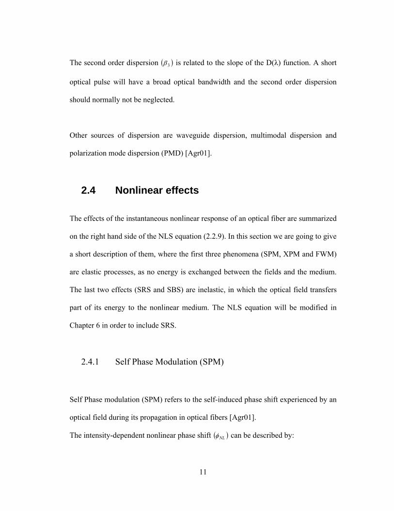
The second order dispersion ( )3β is related to the slope of the D(λ) function. A short
optical pulse will have a broad optical bandwidth and the second order dispersion
should normally not be neglected.
Other sources of dispersion are waveguide dispersion, multimodal dispersion and
polarization mode dispersion (PMD) [Agr01].
2.4 Nonlinear effects
The effects of the instantaneous nonlinear response of an optical fiber are summarized
on the right hand side of the NLS equation (2.2.9). In this section we are going to give
a short description of them, where the first three phenomena (SPM, XPM and FWM)
are elastic processes, as no energy is exchanged between the fields and the medium.
The last two effects (SRS and SBS) are inelastic, in which the optical field transfers
part of its energy to the nonlinear medium. The NLS equation will be modified in
Chapter 6 in order to include SRS.
2.4.1 Self Phase Modulation (SPM)
Self Phase modulation (SPM) refers to the self-induced phase shift experienced by an
optical field during its propagation in optical fibers [Agr01].
The intensity-dependent nonlinear phase shift ( )NLφ can be described by:
11

22
2 ELnNLr
λπφ = (2.4.1)
Where L is the fiber length and Er
the module of the electrical field at the working
wavelength.
Generally SPM brings a broadening of the amplitude spectrum and thus a stretching
of the pulse in time domain. The final result depends on the frequency chirp of the
original pulse as detailed in [Agr01].
2.4.2 Cross Phase Modulation (XPM)
Cross Phase Modulation (XPM) refers to the nonlinear phase shift induced by other
fields, having a different wavelength, direction, or polarization state:
( )22
212 22 EELnNL +=
λπφ (2.4.2)
In this case the term depending on 1Er
is the SPM as in (2.4.1) and 2Er
represent the
external field.
XPM is responsible for asymmetric spectral broadening of co-propagating optical
pulses.
2.4.3 Four Wave Mixing (FWM)
12

When several optical signals at different frequencies propagate along the fiber, the
total electrical field is equal to the vectorial addition of each individual field. The
resulting optical intensity will have new components as a result of the cross products
in the module calculation.
For example if three optical frequencies (f1, f2 and f3) interact in a nonlinear medium,
they will give rise to a fourth frequency (f4), where:
3214 ffff −+= (2.4.2)
FWM is responsible for inter-channel crosstalk in a WDM communication system.
2.4.4 Stimulated Raman Scattering (SRS)
Raman Scattering is an inelastic process where a photon of the incident field (called
pump) is absorbed and reemitted again, via an intermediate electron state, in a lower
frequency. The excess energy and impulse is dissipated as a phonon (vibrational
energy) into the material. This process can be combined with stimulated emission
where the new photon has the same frequency and momentum as an incident signal
photon. Consequently, through SRS, pump photons are progressively destroyed while
new photons, called Stokes photons, are created at a down-shifted frequency that
correspond to the signal photon. Figure 2.1 shows the scheme of the process.
13

2 x hυs hυp hυs
hυp - hυs
hυp hυs
Figure 2.1: Stimulated Raman Scattering, two incident photons, one representing the signal (υs) and the other representing the pump (υp). At the output the signal is amplified, the energy loss is h(υp- υs).
A less probable phenomenon is the emission of an anti-Stoke photon which has
higher energy that the incoming pump. In this study, we will mainly focus in the
generation of Stokes photons through SRS.
SRS has applications in amplification of optical communication signals and
spectroscopy. As a vibrational contribution, the SRS has a delayed response
characteristic for each material.
The relationship between the pump and the signal power (Ip and Is) can be described
as:
spRs IIg
dzdI
= (2.4.3)
Where gR is the Raman gain that can be measured experimentally. The Raman gain
bandwidth is very wide (around 13THz) and thus the effect is particularly important
for large bandwidth signal (very narrow pulses in time domain).
14

SRS is only visible when the pump power exceeds a certain threshold level
(typically ). WPthp 1≈
Spontaneous Raman Scattering occurs when a Raman photon is generated from a
pump photon but without any relationship with the signal. This effect is normally
considered as noise.
2.4.5 Stimulated Brillouin Scattering (SBS)
This effect is very similar to the previous one, but in this case an acoustic phonon is
generated only in the backward direction. SBS has higher but narrower gain (less than
100MHz) then SRS. In optical communication systems, SBS will limit the total
amount of power in the fiber. Because it only propagates in the backward direction
and due to its very narrow gain, we will not consider SBS in this work.
2.5 Split Step Fourier Method
Equation (2.2.7) can only be solved numerically. The preferred method is the “Split
Step Fourier Method”, where dispersion and nonlinear effects are solved separately in
time domain the first one and in frequency domain the last one [Agr01].
The fiber is chirped in small sections, where the dispersion is considered along each
segment, while the nonlinear operator is only applied at each segment’s middle point.
15

This method is implemented by the simulation software VPItransmissionMaker in
which the numerical results of this work are based [VPI05].
16

Chapter 3: Optical Solitons
In this chapter we will give an overview of optical solitons, describing its historical
origins and some fundamental properties. We will also cover some soliton categories
of particular interest for this work.
3.1 Solitons in Physics
Solitons, also known as “solitary waves”, have been the subject of intense studies in
many different fields, including hydrodynamics, nonlinear optics, plasma physics and
biology [Agr03].
The first observation of a solitary wave was in 1834. John Scott Russell, a Scottish
naval engineer, was riding a pair of horses along a narrow channel when he observed
a wave that would continue its course without apparent change of form or speed.
When working in nonlinear optics, solitons are classified as temporal or spatial
depending if they maintain their shape while propagating or if they are confined to the
transverse plane (orthogonal to the propagation direction). In this work we will only
consider temporal solitons which are formed thanks to compensation of the group-
delay dispersion by the self phase modulation (SPM).
17

3.2 Fiber Solitons
Temporal Solitons in optical fibers were first predicted in 1973 [Agr03], and have
several applications in the field of optical communications.
The goal is to find a solution for the NLS equation (that we will call soliton solution),
in which the input pulse maintains its shape as it propagates: ( ) ( ) .,0, ztAtzA ∀=
We can re-write equation (2.2.8), without considering fiber losses, using the soliton
variables:
0
1
Tzt β
τ−
= (3.2.1)
DLzZ = (3.2.2)
ALu Dγ= (3.2.3)
Where T0 is a temporal scaling parameter (normally the input 1/e intensity pulse
width) and 22
0 βTLD = is the dispersion length. The time variable (τ) travels at the
group velocity. The resulting equation for silica fibers is:
uuusignZui 2
2
22
2)(
+∂
∂=
∂∂
−τ
β (3.2.4)
The sign of the dispersion parameter plays an important role in determining the
soliton solution. For normal dispersion (β2>0), optical fibers can support dark solitons
18

where the pulse has zero amplitude at its center. Consequently, in order to support
bright solitons, the GVD needs to be anomalous (β2<0).
Using the inverse scattering method we can find a soliton solution for (3.2.4) which
has the following expression for its initial pulse envelope:
( ) ( )ττ hNu sec,0 = (3.2.5)
Where the parameter N is the soliton’s order and is related to the input pulse and the
fiber parameters as:
DTPcTP
LPN D
200
22
200
02 2 γ
λπ
βγ
γ === (3.2.6)
In a hyperbolic-secant pulse as in (3.2.5) we can relate its 1/e intensity pulse width
(T0) and its Full Width Half Width pulse width (TFWHW) as:
( ) 00 763.121ln2 TTTFWHW ≈+= (3.2.7)
For a Fourier-Transform (FT)-limited pulse the product of frequency uncertainty and
temporal uncertainty is minimized. For these pulses all the information is located on
its amplitude. The Frequency and time width are related as:
21
=∆∆ tω (3.2.8)
Which for a sech2 pulse it can be re-written as:
315.0=∆ FWHWTυ (3.2.9)
Normally, standard solitons are unchirped in the absence of Stimulated Raman
Scattering (IRS) and consequently they are transform-limited. However, the chirp-
free nature is not ensured when their spectrum shifts because of IRS [Agr03].
19

3.3 Fundamental Soliton
The fundamental order or first order temporal soliton correspond to the N=1 case. It is
the only solution that maintains its shape in every moment. The pulse shape is given
by:
( ) 2sec),( iZehZu ττ = (3.3.1)
The fundamental soliton condition can also be understood as the solution where the
nonlinearity (particularly the SPM) compensates the fiber dispersion in every point
along the fiber. Thus, the dispersion length (LD) and the nonlinear length
( ) are always equal. ( ) 10
−= PLNL γ
3.4 Higher Order Solitons
When N>1 in (3.2.5), we have a higher order soliton. Instead of maintaining its shape
over the entire fiber, higher order solitons have a periodical behavior in the z direction
with period [Agr03]:
2
2
2
20
0 222 ββππ FWHW
DTT
Lz ≈== (3.4.1)
3.5 Soliton Interaction
The presence of other pulses in the neighboring perturbs a temporal soliton simply
because the combining optical field is not a soliton solution of the NLS equation. This
20

phenomenon is called soliton interaction and can cause the pulses to come closer or
move apart in time domain.
Soliton interaction is critical for high speed soliton communication systems. In our
case, it occurs between the fundamental and the high order solitons in the fiber.
3.6 Loss-Managed Solitons
In section 3.2 we found a soliton solution for the NLS when the fiber had no loss. In
more general case, while propagating a soliton will lose part of its energy.
Consequently, the pulse will broaden as the SPM is weakened and can no longer
counteract the GVD.
Optical Amplifiers can be used for compensating fiber losses. Two techniques have
been proposed: the Lumped Amplification, where optical amplifiers (generally EDFA)
are placed periodically along the fiber, causing a sort of average compensation effect;
and Distributed Amplification which provides nearly lossless fibers by compensating
losses locally at every point. This objective is achieved by using Raman Amplifiers
[Mol85]. In both solutions the location and gain of the amplifiers are key design
parameters.
21

3.7 Dispersion Management Solitons (Average Solitons)
Dispersion management is widely used in WDM systems by employing specially
designed fibers. Optical solitons benefit from this technique as power losses can be
overcome by modifying the dispersion parameter in order to satisfy (3.2.6).
Fundamental solitons can be maintained in a lossy fiber if its GVD decreases
exponentially as:
( ) ( ) zez αββ −= 022 (3.7.1)
Fibers with such a GVD have been fabricated and are called Dispersion-Decreasing
Fibers (DDF). Their main characteristic is the reduction of the core diameter along
the fiber length. A disadvantage of DDF is that the average dispersion along the fiber
links is normally large.
Another solution for compensating the fiber losses by dispersion management
consists of using a dispersion map. In this case, a map period is formed by a
concatenation of a positive dispersion fiber and a negative dispersion fiber. Even
though the local dispersion does not agree with (3.7.1), the average dispersion over a
map period does.
At first sight, normal dispersion fibers (D<0) do not support bright solitons and this
solution should not work. Nevertheless, it has been shown that when the map period
22

is a fraction of the nonlinear length, nonlinear effects are relatively small and the
pulse evolves in a linear fashion over one map period. In this case the SPM is
compensated by the average dispersion. As a result the solitons’ peak power, width
and shape will oscillate periodically [Agr03].
Long distance transmission of an average soliton has been demonstrated by [Gri00].
In that experiment a 10-GHz pulse train propagated along a 28000 km re-circulating
loop with near zero average dispersion. The dispersion map consisted of 100km of
dispersion-shifted fiber (D= -1.2ps/nm/km) and 7km of standard fiber (D= 16.7
ps/nm/km). Amplifiers were placed every 25km.
23

Chapter 4: Short Pulsed Fiber Lasers
Fiber lasers have been available since 1961 [Agr201] as an alternative for solid state
short-pulses lasers. As in any laser, we can identify three main components: an optical
cavity, a pump and a gain medium (that performs the population investment).
Since 1989, Er+3 doped fiber-lasers have kept most of the attention as they can be
used on the 1550nm telecommunication windows. Other rare earth materials, such as
Yb+3 or Nd+3, are used for high power lasers.
The first fiber lasers were continuous-wave (CW), but since the late 80s pulsed lasers
have been built using a mode locking technique.
This chapter will give a quick review to some basic laser concepts and to solid state
lasers. We will then show some typical configurations for fiber lasers.
4.1 Short Pulsed Cavity Lasers
It could look contradictory, a priori, to generate ultrashort pulses with a laser source,
because of the frequency selection imposed by the optical cavity. Normally, these
cavities will allow oscillations in a few very narrow frequency domains around the
discrete resonance frequency: Lqcq 2=υ (q is an integer, c the speed of light and L
24

the optical length of the laser cavity) [Rul03]. Consequently, it can not deliver
ultrashort pulses while working in its usual regime.
In order to obtain a pulsed laser, the cavity needs to work on the multimode regime,
where all the longitudinal modes of the laser (where the unsaturated gain is greater
than the cavity losses) exist simultaneously. The time distribution of the laser output
depends essentially on the phase relationship between the different modes.
4.2 Mode-locking
While operating in a multimode regime, there is usually a competition between modes
to be amplified by stimulated emission from the same atoms, molecules or ions. This
contest brings fluctuation on the output instantaneous intensity, where the worst
scenario is a totally random noisy signal.
By organizing the mode competition, the mode-locking technique tries to obtain
periodic pulses at the output of the laser source; in frequency domain, the problem
could be formulated as finding constant relative phases between modes.
Mode-locking will normally be achieved by inserting a nonlinear material in the
cavity. In time domain, as the wave travels back and forward into the cavity, each
time it goes through the nonlinear material, the stronger fields will be considerable
25

more amplified than the weaker fields. If the conditions are well chosen, the situation
can arise to have all the energy concentrated in one single pulse.
There are two major classifications of mode-locking: passive and active. However, in
some occasions a self-locking process is possible, if the following conditions are
fulfilled:
- The pulse regime is favored over the CW regime.
- The overall system possessing the property of shortening the pulses
(normally by Kerr effect).
- Some mechanism initiating the self-locking process (for example knocking
the table or randomly moving some element in the cavity).
4.2.1 Active Mode-locking
Active mode-locking consist of modulating the amplitude of each longitudinal mode
by changing the cavity losses or the gain of the amplifying medium through an active
element introduced inside the fiber cavity. The first effect can be achieved by using
an acoustic-optical crystal and the second by pumping the medium with another
mode-locked laser.
4.2.2 Passive Mode Locking
26

If an absorbing medium with a saturable absorption coefficient (normally a liquid dye
solution) is placed inside the cavity, the combination of this material and the saturable
amplifying medium leads to the natural mode-locking of the laser. This process is
called passive mode locking which has no external monitoring or feedback circuit.
The pulse reaches its final shape when it becomes self-consistent in the cavity, which
means, when it keeps the same shape after a round trip.
The main problems with passive mode locking are: first, there are many compatible
pairs of saturable absorbing and amplifying media with the right properties. Secondly,
the output pulses are not very powerful and their wavelength is not easily tunable.
The hybrid method tries to take the best from the two previous ones in order to obtain
a wider choice of wavelengths and powers. In this case, the saturable absorber is
introduced inside a cavity with an external modulator, making it easier to obtain sub-
picoseconds pulses than the classical active mode-locking.
4.3 Solid State Laser
A Solid State Laser uses a solid crystalline material as the gain medium and is usually
optically pumped. They should not be confused with semiconductor or diode lasers
which are also ‘solid state’ but are almost always electrically pumped.
27

In recent years, most of the work in the field of ultrashort light pulse generation have
been based on the development of titanium-doped aluminum oxide (Ti:Al2O3,
Ti:sapphire) as a gain medium. The emission band of these lasers is centered in the
red region (~750nm) and can be tuned as much as 200nm [Rul03].
Even though active or passive mode-locking can be implemented, self-mode-locking
has shown to be the best choice. Normally a Kerr lens acts as the nonlinear medium in
order to achieve the locking property. The laser may need an additional external
cavity to improve its stability. Figure 4.1 shows a typical setup for a Ti:sapphire laser.
Figure 4.1: Ti:Sapphire laser setup with Argon CW pump and self-mode-locking. Fig 3-23 [Rul03].
The pump source can be an argon-ion CW laser (normally of about 10W of CW) or a
diode pumped green emitting laser. The length of the crystal is in the order of 1cm.
These kinds of lasers can generate 10fsec pulses at repetition rates of around 80Mhz.
28

4.4 Fiber Lasers
A quick overlook to figure 4.1 shows that Solid State lasers have several
mechanically adjustable optical elements that make it difficult for a commercial
implementation outside the optical table.
A fiber amplifier can be converted into a laser by placing it inside a cavity designed
to provide optical feedback. In this case the cavity is formed by optical fibers,
couplers and mirrors, the doped fiber acts as the gain medium, and a CW diode laser
as pump.
The selection of the pumping laser for a fiber laser will depend on the dopant and the
laser threshold for the system. Pumping schemes can be classified as three-level, four-
level or up-conversion lasers [Agr201].
Fiber lasers have the following advantages:
- Simple doping procedure.
- Low loss and high efficiencies.
- Pumping by compact and efficient diodes.
- An all-fiber device minimizing the need of mechanical alignments.
- Mode-locking, simplified thanks to the long interaction length.
- Lower cost
29

Erbium doped fiber lasers work in the 1550nm region, which is ideal for long
distances transmission. However, and thanks to the use of Periodically Poled Lithium
Niobate (PPLN) waveguides, efficient 780nm lasers are feasible through frequency
doubling [Arb97].
Nonlinear effects, such as XPM and SPM, play a central role in the operation of a
fiber laser, especially in the achieving of mode-locking. Dispersion causes the
broadening of the output pulse.
Fiber lasers can be configured for active or passive mode-locking, where the second
option is normally simpler and cheaper. Two cavities designs are relevant: ring cavity
and linear Fabry-Perot cavity. We will describe them in the next sections.
4.4.1 Ring Cavity Fiber Lasers
A simple ring fiber laser is shown in Figure 4.2, where the isolator works as the
nonlinear medium. The repetition period is equal to the time needed to complete one
round over the ring.
30

980 nm Pump
1550 nm Output
WDM Coupler
90/10 Coupler
Single-mode fiber
Erbium-doped fiber
Polarization Controller
Isolator/Polarizer
Figure 4.2 All-fiber ring-laser. An isolator works as a polarizer in the forward direction and blocks the light propagation in the reverse direction [Nel97].
In a passive mode locking configuration, the pulse shortening is performed by the
coherent addition of self-phase modulated pulses, thus it is very fast. We explain this
process in Figure 4.3; a pulse with arbitrary polarization is elliptically polarized by
the use of a polarizer and a quarter-wave plate. The nonlinear medium will cause the
pulse peak to rotate its polarization more than the pulse’s edges. The last two
elements (a half-wave plate and an output polarizer) filter the low intensity
components, making the overall effect a stretch of the original pulse. The input and
output polarizers are adjustable, and will be useful for the starting process.
Non Linear Element
Output narrower pulse
Polarizer λ/2 λ/4 PolarizerInput wide pulse
Figure 4.3 Pulses Shortening in a Ring Fiber Laser [Nel97].
31

Ideally, a passive mode-locked laser will evolve into a pulsed state on its own,
without an external perturbation or trigger. This is called “self-starting”, where the
pulses start up from the initial noise fluctuations. A mode-locked state can only be
achieved if the gain experienced by the fluctuation is long enough to allow it to
complete a round trip within its lifetime [Nel97]. Lasers in a unidirectional ring
configuration have shown to self-start easily with relative low powers.
4.4.2 Fabry-Perot or Linear cavities
Another configuration for fiber lasers are linear cavities, where the gain medium is
placed between two high-reflecting mirrors. Alignment of these cavities is not easy as
cavity losses increases rapidly with a tilt of the fiber end or the mirror. This problem
can be solved by depositing dielectric mirrors directly onto the fiber ends.
Dielectric coating can be damaged by the high power pump. Consequently, several
alternatives exist including the use of WDM couplers, Bragg gratings or fiber-loop
mirrors.
Figure 4.4 shows a schematic for a fiber laser with a saturable Bragg reflector used
both as one edge of the cavity and as the non-linear element that allows the passive
mode-locking.
32

980nm pump in
WDM Coupler Er/Yb doped fiber
SMF
Connector with a dielectric mirror
SBR
1550nm out
Figure 4.4: Schematic of a fiber laser where a Bragg reflector is used also for mode locking [Agra201].
Linear-cavity lasers will normally need between 10 to 100 times more powers than
ring-lasers for self-starting.
4.5 High Power Pulsed Fiber Lasers
Single-mode fibers can not handle very high peak power signals due to their small
fundamental mode area. In order to solve this problem, several techniques have been
developed including cladding pumped lasers and cladding pumped holey fiber lasers.
Multimode fibers (MMF) are well known for its large area, and thus are a feasible
medium for high power fiber lasers (MMF can handle up to 30 times larger power
than SMF). However, when using MMF there are several problems derived from the
interaction between modes: multimode dispersion, mode coupling, an increase in
generated amplified spontaneous emission (ASE) power noise, etc.
33

Ideally, we would like to preserve single mode propagation in the MMF. This could
be checked by splicing a MMF in between two single-mode fiber filters and
measuring the insertion loss as a function of the MMF length. For a silica fiber with a
cladding diameter of 250µm and a core diameter of 50µm, single-mode propagation
can be preserved over lengths shorter than 20m. Also, in such fibers mode-coupling is
relative insensitive to fiber bends [Fer00].
Figure 4.5 shows an experimental setup for a diffraction-limited passively locked
(through a saturable absorber) MM fiber laser. In this case the pulse stretching is
achieved by the use of two Faraday rotators and a fixed polarizer.
Pump
Doped MM fiber
Partial reflection
Faraday rotator
Faraday rotator
Saturable absorption mirror
PPLN
780 nm Output
Figure 4.5: MM fiber oscillator side-pumped with a broad-area laser diode [Fer00]. A PPLN is introduced at the edge to frequency double the output signal.
34

Chapter 5: Photonic Crystal Fibers
5.1 Fundamentals of photonic crystal
waveguiding
Photonic Crystal Fibers (PCF), also known as Microstructured Fibers (MF) or
Microstructured Optical Fibers (MOF) [Bja03], represent one of the most active
research areas in optics. Their main characteristic is the presence of a periodic or
aperiodic structure (particularly air holes) in the core-cladding area of the fiber.
Optical applications for periodic structures are well known in nature, a classical
example are the colorful spots on several butterfly’s wings; as the insect moves them,
we can appreciate the spots changing color [Bja03].
One Dimensional (1D) periodic structures, or one dimensional photonic crystals (PC),
are extensively used for important applications in optics, such as diffraction gratings,
Bragg stacks, etc.
Fiber optics and waveguides propagation usually relies on internal reflection or index
guiding. However, PCF, which are a 2D array, normally rely on the bandgap effect.
This phenomenon, similar to the recombination of a electron-hole pair in a
35

semiconductor, inhibits the electromagnetic field to propagate with certain
frequencies, forming a bandgap.
5.2 Classification of PCF
Different applications of PCF have different requirements in the fabrication process.
When observing its profile we can vary the number, size, form and position of the
holes. For some applications it is also important to dope the core in order to dominate
the attenuation and dispersion. Figure 5.1 shows the most used terms and major
classes of PCF.
Photonic Crystal Fiber (PCF) Microstructured Fiber (MF) Microstructured Optical Fiber (MOF)
Main class I Main class II - High-Index Core Fiber - Photonic Bandgap Fiber - Index Guiding Fiber - Bandgap Guiding Fiber - Holey Fiber
Figure 5.1: Classification of PCF [Bja03].
Hollow-Core (HC) or Air Guiding (AG)
High NA (HNA)
High Non linear (HNL)
Large Mode Area (LMA)
Low-Index Core (LIC)
Bragg Fiber (BF)
36

Only the fibers on the Main Class II propagate thanks to the bandgap effect, while the
rest are index-guiding fibers.
HNL are especially relevant for this work. These fibers normally have few holes
located in the cladding area and a very small (~2µm) core diameter.
5.3 Modeling of microstructured fibers
Two dimensional photonic crystals are the most studied case of periodical structures
[Bja03]. Figure 5.2 shows an axial cut of a PCF where for simplicity a hexagonal
representation is chosen. In this example we have a background material (normally
SiO2) and cylinders of diameter d arranged in a hexagonal lattice with a period Λ.
Most fiber parameters will depend on the factor d/ Λ.
d
Λ
Figure 5.2: Geometrical characteristics of PCF.
Cylinders normally contain just air, but eventually they can be filled with gasses or
other substances in order to build an optical sensor.
37

When modeling a Photonic Bandgap Fiber, the full vectorial nature of the
electromagnetic waves has to be taken into account. A simulation software developed
by MIT is widely used by the research community [MIT04].
On the other hand, when working with Index Guided Fibers, it is possible to apply the
methodology developed for standard fibers by calculating an effective index for the
cladding. The idea is to replace the PCF by an equivalent step-index fiber, where the
core is pure silica and the cladding has a refraction index that considers the geometry
of the PCF. The calculation of the core radius of the equivalent step-index fiber, as
well as other numerical methods for modeling PCF can be found in the literature.
[Bja03]
When considering HNL-PCF, its Raman gain coefficient will vary from a standard
fiber. There are two factors that affect this coefficient, first the smaller effective area
(less than 10µm2). Second, the existence of air holes where no Raman Effect can
occur. The numerical calculations for both parameters from the geometrical
characteristics of the fiber are shown in [Fuo03].
38

5.4 Fabrication of photonic crystal fibers
The idea of producing optical fibers with microscopy air holes goes back to the early
days of optical fiber technologies.
As in the standard fiber, PCF fabrication consists of two main steps: the preform
production and the drawing process using a high temperature furnace in a tower set-
up.
It is not desired to build a preform by drilling every hole in the bulk silica. However,
the product is obtained by directly staking silica tubes and rods with a circular outer
shape. Employing circular elements introduces additional air gaps in the fiber preform.
These could be avoided by using hexagonal elements, but in that case the
manufacturing process would be more complex. For air core fibers, the center rod is
replaced by capilar tubes that will break during the drawing process, forming an
empty core structure. After stacking, the capilars and rods may be held together by
thin wires and fused in an intermediate process, forming preform-canes.
One of the main disadvantages of the stack and pull technique is the contamination of
the glass elements. In recent years, other fabrication methods such as extrusion of the
core preform have been introduced.
39

The drawing of PCF is done in conventional towers. In order to avoid the collapse of
air holes due to its low surface tension, low temperatures are used (around 1900oC).
The key element of this process is to keep the fiber regular structure from the preform
up to the fiber dimension.
5.5 Applications
The most popular PCF are the High Nonlinear Fibers (HNL). They can achieve a high
non-linear coefficient and a positive dispersion parameter in the visible region,
allowing the formation of optical solitons. This effect is used to build highly
wavelength-tunable fiber lasers, with short fiber lengths. HNL fibers are also used for
supercontinuum (500 to 1700nm) generation, which has applications in metrology
(frequency references), coherence tomography and spectroscopy. When the zero-
dispersion wavelength is shifted at 1550nm, HNL fibers are very attractive for
telecom applications such as 2R Regenerators, multiple clock recovery, pulse
compression, wavelength conversion and supercontinuum WDM sources.
Double claddings PCF are of predominant interest in the context of high power
devices. Normally the fiber is doped with rare-earth elements such as Yb3+ and Nd3+.
These fibers have a high numerical-aperture, permitting an effective coupling of the
pump power.
40

Air guiding fibers can be used as the active medium for optical sensors, where the
core can be filled with the target gas or biological species.
41

Chapter 6: Experimental and Numerical Analysis of Soliton Self-Frequency Shift
The goal for this Chapter is to build and simulate a wavelength shifter to be used in
conjunction with a pulsed fiber laser as a pump for two photons microscopy. We will
show the complete setup in Chapter 8. Similar systems were reported in [Nor99] and
[Nor02]. However, there have been no reports of the use of these sources for two
photon imaging.
We will first introduce the experimental setup and show the resulting spectrums. We
will then generalize the NLS equation in order to include the Raman scattering.
Through the numerical analysis we will show the pulse evolution while propagating
along the optical fiber.
6.1 Experimental Results
The experimental setup is shown in Figure 6.1. The pump is a pulsed fiber laser
(IMRA Femtolite Ultra) which transmits 100fsec pulses in the 780nm wavelength at a
repetition rate of 50MHz and a maximum output average power of 20mW. The non-
linear medium consisted of 7m HNL-PCF (Photonic Crystal Fiber NL-18-710). The
fiber parameters are detailed in Appendix A. The fiber’s zero-dispersion wavelength
42

is 710nm. For the selected pump, the fiber is working at the anomalous dispersion
region as needed to generate bright solitons.
The power launched into the fiber was adjusted by mechanically misaligning the
optical system. The signal at the output of the fiber was coupled into an optical
spectrum analyzer (ANRO AQ6317B).
PCF
780 nm fiber laser OSA Mechanic
Translator
Figure 6.1: Experimental Setup for a Wavelength-Tunable Pulsed Laser Source.
When the incoming pulse has low average power, the chromatic dispersion is the
predominant effect and the pulse is simply broadened when traveling trough the fiber.
As we increase the input power, the SPM effect decreases the amount of total
broadening of the original pulse. After exceeding the Raman threshold, the pulse will
change its central frequency thanks to the SRS in a process known as pulse self-
frequency shift (PSFS) [Zys87].
After an initial stage of narrowing and when the incoming pulse exceeds a certain
threshold (in our case 200µW of average power), the pump pulse brakes into two
pulses by a phenomenon described by Zysset et al [Zys87] [Bea87]. The generated
pulse is formed at the longer-wavelength side of the pump (also called Stokes bands)
43

and forms a fundamental soliton. The center wavelength of this soliton is shifted as
the soliton propagates along the optical fiber. The shifting process is called soliton
self-frequency shift (SSFS) and is a result of the SRS. The amount of frequency shift
will depend on the pump peak power and the fiber length. Figure 6.2 shows the
experimental spectrum obtained for the setup in Figure 6.1 while varying the
launching power.
750 800 850 900 950 1000 1050Wavelenght (nm)
Arb
itrar
y un
its (a
u)
Figure 6.2: Experimental spectrums for a wavelength shifter where a mechanical translator is used to vary the input average power as shown in figure 6.1.Different colors correspond to different input
powers.
44

We can observe in figure 6.2 that the fundamental soliton is shifted over 1µm, but a
second order soliton is formed from the remaining power of the original pulse when
the fundamental soliton is above 920nm.
6.2 Generalized Non-Linear Schrödinger
Equation
In this section we will generalize the NLS equation in order to explain the
experimental results of the previous section. Although equation (2.2.8) explains most
of the common nonlinear effects in an optical fiber, it does not include the SRS which
origins the SSFS.
Intra-pulse Stimulated Raman Scattering is related to the delayed nature of the
vibrational response of the SiO2 molecules. Thus, mathematically, we need to use the
most general form for the nonlinear polarization given in equation (2.1.6) assuming
the following functional form for the third-order susceptibility:
( )( ) ( ) ( ) ( ) ( )3213
3213 ,, ttttttRtttttt −−−=−−− δδχχ (6.2.1)
Where R(t) is the normalized nonlinear response function. It includes both the
electronic and the vibrational (Raman) contributions. Assuming that the electronic
contribution is instantaneous, R(t) can be written as [Sto89] [Sto92]:
( ) ( ) ( ) ( )thftftR RRR +−= δ1 (6.2.2)
45

Here fR represents the fractional contribution of the delayed Raman response to the
nonlinear polarization and hR(t) is the Raman response function which is responsible
for the Raman gain whose spectrum is given by:
( ) ( ) ( )[ ]ωχω
ω ∆=∆ RRR hfcn
g~
Im3
0
0
(6.2.3)
The Raman gain can be found experimentally as shown in [Sto92]. The real part of
is found by using the Kramers-Kronig relations. Figure 6.3 shows the
temporal variation of h
( ω∆Rh~ )
R(t) and Figure 6.4 shows a typical Raman gain for a SiO2 fiber.
We should note that hR(t) becomes nearly zero for pulses wider than 5ps.
Figure 6.3: Raman Response Function [Agr01].
46

0 5 10 15 20 25 30 350
0.1
0.2
0.3
0.4
0.5
0.6
0.7
0.8
0.9
1
Frequency Shift (THz)
Nor
mal
ized
Ram
an G
ain
Figure 6.3: Normalized Raman Gain for a SiO2 fiber. The maximum value is at THz2.13=∆υ (equivalent to nm7.26=∆λ ) when the central frequency is 780nm [VPI05].
A common analytical approximation for the Raman response function is:
( ) ( ) ( 1221
22
21 sin2 τ
ττττ τ teth t
R−+
= ) (6.2.4)
The parameters τ1 and τ2 are adjustable for a good fit to the experimentally known
gain spectrum. The generally accepted values are: τ1=12.2fsec, τ2=32fsec and fR=0.18.
By considering equation (6.2.1), the new expression for the nonlinear Schrödinger
equation is generalized to include the Raman scattering as:
( ) ( ) ( ) ( ) ( ) ⎟⎟⎠
⎞⎜⎜⎝
⎛−⎟⎟
⎠
⎞⎜⎜⎝
⎛∂∂
+=∂∂
−∂∂
+∂∂
++∂∂
∫+∞
∞−
'',',161
222
03
3
32
2
21 dtttzAtRtzAt
iitA
tAi
tAA
zA
ωωγβββωα
(6.2.5)
47

The accuracy of this equation is verified by showing that it preserves the number of
photons during the pulse propagation if the fiber losses are set to zero (α=0). The
pulse energy is not conserved as part of the pulse energy is absorbed by the silica
molecules (Raman scattering is inelastic). These nonlinear losses are included in
(6.2.5).
For pulses wide enough to contain many optical cycles (widths>>10fsec), we can use
a Taylor-series expression for the pulse envelope:
( ) ( ) ( ) 222 ,',', tzAt
ttzAttzA∂∂
−≈− (6.2.6)
Another simplification consists on defining the first moment of the nonlinear
response function as:
( ) ( ) ( )( )
0
~Im
=∆
∞
∞−
∞
∞− ∆=== ∫∫
ωωdhd
fdttthfdtttRT RRRRR (6.2.7)
The result in the Schrödinger equation is:
( )⎟⎟
⎠
⎞
⎜⎜
⎝
⎛
∂
∂−
∂∂
+=∂∂
−∂∂
++∂∂
TA
ATAAT
iAAiT
AT
AiAzA
R
22
0
2
3
3
32
2
2 61
22 ωγββα
(6.2.8)
In this case the time frame moves with the pulse at the group velocity:
ztztT g 1βυ −≡−= (6.2.9)
Equation (6.2.5) is the most generic NLS formulation where the complete solution
can only be found numerically using, for example, the Split-Step Fourier Method as
explained in Chapter 2.
48

6.3 Numerical Analysis
In order to understand the experimental results obtained in section 6.1 we will
numerically solve equation (6.2.5) for different input powers and fiber lengths.
The numerical calculations were done using the software VPItransmissionMaker
[VPI05] where the numerical parameters are detailed in Appendix B. The fiber
parameters are the same as in the experimental setup and are shown in Appendix A.
As it was already mentioned, when the input optical average power exceeds 200µW,
the original power is breaking into two pulses creating an optical soliton. Figure 6.5
shows the numerical simulation of the formation of this soliton over the “wide” pump
pulse in time domain.
49

-0.4 -0.2 0 0.2 0.40
20
40
60
80
100
120
140
Time (psec)
Pow
er (W
)
Figure 6.5: Soliton formation from the original pump pulse through pulse break-up. The input pulse was 300µW of average power and 0.5m of HNL-PCF.
While propagating along the fiber, the new pulse (a soliton) is shifted in frequency.
The Soliton Self-Frequency Shift (SSFS) was first observed by L.F.Mollenauer, et al.
[Mol85] and analytically described by Gordon [Gor86]; this will be detailed in
Chapter 7. The magnitude of the wavelength shift is dependent upon the fiber length
and the pump power. These two dependencies will be studied in this section.
50

The first analysis consists of studying the time (Figure 6.6) and spectrum (Figure 6.7)
characteristics at the output of 7m of HNL-PCF when the average input power is
modified.
-20 0 20 40 60 80 100Time (psec)
1500µW
1200µW
1100µW
1000µW 900µW
800µW
600µW 500µW
400µW 300µW 200µW
Figure 6.6: Time domain Characteristics of the output from a 7m HNL-PCF for different input average power.
Soliton formation in a HNL-PCF was first predicted by Reid et al in [Rei02]. In our
simulation, the fundamental soliton is generated when the input average power is
200µW and the second order soliton when it is 800 µW, which agrees with equation
(3.2.6). After the soliton is generated it rapidly shifts its central wavelength.
51

1500µW
1200µW
1100µW
1000µW
900µW
800µW
600µW
500µW
400µW 300µW
100µW 200µW
700 750 800 850 900 950 1000 Wavelength (nm)
Figure 6.7: Wavelength Shift for different Input Average Power in a 7m HNL-PCF.
It can be observed in the time domain analysis (Figure 6.6) that the fundamental
soliton is delayed with respect to the pump pulse. This delay has two components: the
group delay dispersion and the delayed nature of the Stimulated Raman Scattering. If
we suppose a dispersion parameter of D = 68 ps/nm/km and a bandwidth of 10nm, the
delay due to the linear dispersion would be: psT 5007.01068 =××=∆ . Consequently,
the delay shown in figure 6.6 is mainly due to the Raman Effect.
52

Figure 6.7 shows that it is possible to build a wavelength shifter without second order
generation in the range of 780 to 920nm. Further shift is possible if we filter these
lower wavelength components.
Figure 6.8 shows how the wavelength shift evolves when we vary the input average
power for 3m and 7m of HNL-PCF. This study was done by [Nor99] for a
polarization maintaining fiber. For low input power the group delay dispersion
dominates and there is no soliton formation. As the power increases, the fundamental
soliton is formed and shifts its central wavelength linearly until it reaches a saturation
behavior. This is caused by both the fraction of power taken by the second order
soliton and the wavelength dependency of the fiber parameters. The effect of the fiber
parameters on the soliton self-frequency shift is analyzed in Chapter 7.
53

0 200 400 600 800 1000 1200 14000
20
40
60
80
100
120
140
160
180
Input Average Power (uW)
Wav
elen
gth
Shi
ft (n
m)
3m HNL-PCF7m HNL-PCF
Figure 6.8: Wavelength Shift and Input Average Power for 3m and 7m HNL-PCF.
When the input power reaches certain limit, we can observe the formation of a
supercontinuum (SC) [Ort02]. This phenomenon consists on the considerable spectral
broadening of optical pulses and has applications in the fields of optical
communications, metrology and coherence tomography [Ort02]. The origin to the SC
generation in HNL-PCF is related to the split of higher-order solitons into several
pulses with different red-shifted central frequencies. The non-solitonic pulses
maintain a phase relationship that causes the SC radiation [Por03]. Figure 6.9 shows
the numerical spectrum after applying a 5mW pulse to 7m of HNL-PCF, where a SC
is generated.
54

650 700 750 800 850 900 950 1000-120
-110
-100
-90
-80
-70
-60
-50
-40
-30
-20
Wavelength (nm)
Pow
er (d
Bm
)
Figure 6.9: Supercontinuum generation after applying 5mW pulses to 7m of HNL-PCF.
In figure 6.8 we can also observe that the difference between the wavelength shifts for
3m and 7m of fiber is very small. By studying the dependency of the wavelength shift
on the fiber length, we will also understand how the pulse evolves as it propagates
through the fiber. We perform a numerical simulation for a HNL-PCF varying its
length form 0.1m up to 7m. The results are shown in figures 6.11 to 6.14. In the first
section of the fiber, the chromatic dispersion and the self phase modulation (SPM)
compete between each other causing the narrowing of the original pulse. After the
soliton is formed through the break-up process, it starts shifting its central wavelength.
As it propagates, the soliton suffers the effects of fiber losses and changes on the
55

wavelength-dependent fiber parameters. The consequence of the presence of fiber
losses can be summarized as follows: as the peak power decreases, the width of the
soliton increases in order to maintain the fundamental soliton relationship. The
overall effect is a decrease on the wavelength shift slope as the fiber length increases.
Figure 6.10 shows the time characteristics as a function of the fiber length; we
observe the pulse attenuation and the pulse broadening.
7m
6m
5m
4m
3m
2m
1m
0.5m
0.1m
0 5 25 30 10 15 20Time (psec)
Figure 6.10: Time domain characteristics for different HNL-PCF lengths and an input average power of 500µW. The soliton is form after propagating along over 0.5m of fiber and then is
attenuated and broadened.
In the next two figures we show the evolution of the wavelength shift and the
soliton’s pulse width as a function of the fiber length where both cases agree with the
results of [Nor99] for a polarization maintaining fiber.
56

In Figure 6.11 we can verify the saturation behavior of the wavelength shift as we
increase the fiber length. In the case of an input signal of 1mW average power, a
second order soliton is formed soon after the fundamental soliton. The second order
soliton has a lower peak power that gives a lower shift but it also has saturation
behavior as a function of the fiber length.
0 5 10 15 200
20
40
60
80
100
120
140
160
180
Length (m)
Wav
elen
gth
Shi
ft (n
m)
500µW300µW1mW 1st Order1mW 2st Order
Figure 6.11: Wavelength Shift and Fiber length for a HNL-PCF and different input average powers. For 1mW, we show the 1st and 2nd order soliton shift.
From Figure 6.11 it can be seen that a higher power pump pulse will produced a
narrower soliton. In the next chapter it will be demonstrated that a narrower pulse
width will cause a longer wavelength shift. As the pulse propagates along the fiber, its
57

pulse width is increased in order to maintain the fundamental soliton condition. In
figure 6.13 we show how the soliton order is maintain around N=1 as explained in
[Sto92].
0 5 10 15
110
120
2020
30
40
50
60
70
80
90
100
Fiber Length (m)
Sol
iton
Pul
se W
idth
(fse
c)
500µW300µW
Figure 6.12: Soliton Pulse width and Fiber Length for a HNL-PCF.
We will finally compare the numerical spectrum and the experimental data for 7m of
HNL-PCF detailed in section 6.1. The Input optical power is modified by optical
misalignment as shown in figure 6.1. Figure 6.14 shows the good agreement between
the wavelength shift observed in our experiments and the shift predicted by the
numerical analysis
58

760 780 800 820 840 860 880 900 920Wavelength (nm)
Arb
itrar
y U
nits
(a.u
.)
Numerical Simulation
Experimental
0 5 10 15 200
0.2
0.4
0.6
0.8
1
Fiber Length (m)
Sol
iton
Ord
er
Figure 6.13: Soliton order N and fiber length. Circles represent the values for an input average power of 500µW and the diamonds for 300 µW.
Figure 6.14: Numerical and Experimental Results Wavelength Shifts for the setup in figure 6.1.
59

Chapter 7: Analytical Analysis of Soliton Self-Frequency Shift
Solitons have been introduced in Chapter 3 as a solution for the NLS equation that
preserves the pulse shape as it propagates. In this section we are only going to
consider fundamental order solitons.
Stimulate Raman Scattering will cause a pulse mean frequency to shift toward lower
values while propagating in an optical fiber. In the special case of an optical soliton, it
is possible to formulate an analytical expression for this shift as a function of its pulse
width. However, this expression is only valid while the fiber parameters stay constant
while the pulse is shifting its central frequency.
In this chapter we take a close look at the analytical theory formulated by Gordon
[Gor86] and experimentally confirmed by Mitschke and Mollenauer [Mit86]. We will
then introduce a semi-analytical method for calculating the SSFS when the fiber
parameters are not constant and we will contrast it with numerical calculations for
different fibers.
60

7.1 Analytical Model
Shifts of the mean soliton frequency can only be caused by frequency-dependent
losses or gain in the fiber. The Raman scattering will amplify the lower frequency
components (acting as the signal) at the expense of the higher-frequency parts (acting
as the pump).
Optical Solitons are the solutions of equation (3.2.4) that will not change its shape
while propagating. That normalized equation needs to be generalized in order to
consider the Raman scattering effect in a similar form as in equation (6.2.5):
( ) ( ) ( ) ( ) ( )∫ −+∂
∂−=
∂∂
− 22
2
21 susfdsuu
Zui ττ
τττ (7.1.1)
In this expression we are neglecting the electronic vibrational contributions and all
other nonlinear dispersive terms, f(s) represent the normalized fractional Raman
response function: ( ) ( )shfsf RR= , where f(-s)=0 (due to causality) and . ( )∫ = 1dssf
The Fourier Transform expression for a fundamental soliton as in equation (3.2.5) is:
( ) ( ) ⎟⎠⎞
⎜⎝⎛ Ω
==Ω ∫ Ω
2sec
21~ πττ τ heudu j (7.1.2)
Where ( 00 T)ωω −=Ω is the frequency deviation in soliton units and 0ω the mean (or
central) frequency of the pulse. We can now represent equation (7.1.1) in the
frequency domain (FT):
61

( ) ( ) ( ) ( ) ( )[ ]∫ −+ΩΩ−=∂
Ω∂− 22 ~
21~
susfdsuFTuZ
ui ττ (7.1.3)
( ) ( ) ( )[ ] ( ) ( ) ( )[ ]22 **~ τττ ufFTustusfdsuFT Ω=−∫ (7.1.4)
We introduce the function ( ) ( )[ ] ( )∫ Ω==Ω siesfdsfFT τχ that has the nature of a
susceptibility due to the conditions on f. Returning to our analysis for the NLS
equation in frequency domain and using the Fourier transform properties for the
convolution and the complex conjugate:
( ) ( ) ( ) ( ) ( ) ( )'''~'~'''''~''~21~
*2 Ω+ΩΩΩΩΩ−ΩΩ+ΩΩ−=∂
Ω∂− ∫ ∫ uududu
Zuj χ (7.1.5)
The complex function ( ) ( ) ( )Ω+Ω=Ω ''' χχχ j verifies the Kramers-Kronig relations.
Its imaginary part can be related to a loss coefficient that we will call the Raman
attenuation coefficient ( R )α . To find this relationship, we split the spectrum of our
pulse in two components: the pump (up) and the signal (us). The first one is
considered as a single frequency, constant amplitude signal and the second one is
only a small perturbation:
( ) ( )tueutu sti
pp += Ω− (7.1.6)
( ) ( ) ( )Ω+Ω−Ω=Ω spp uuu ~~ δ (7.1.7)
Substituting (7.1.7) in (7.15), where we only consider the terms proportional to the
pump power and the imaginary part on the right-side terms, we get:
( ) ( ) ( ) 222
~''2~
ΩΩ−Ω−=∂
Ω∂spp
s uuZ
uχ (7.1.8)
We finally obtain an expression for the nonlinear Raman attenuation coefficient:
62

( ) ( ) ( )[ ]∫ Ω=Ω−Ω−=Ω sjpR esfdsIm2''2χα (7.1.9)
After finding a frequency-dependent attenuation, we would like to obtain its
relationship with the central frequency shift. In order to proceed, we will first define
the mean frequency deviation of the soliton as:
∫ ΩΩ>=Ω< 2~udπ (7.1.10)
This magnitude is normally zero, when considering a fundamental soliton. We would
like to evaluate its derivative with respect of the Z position:
( )∫∫ ΩΩ=
ΩΩ=
>Ω<dZud
ddZ
udd
dZd
22 ~~π
π (7.1.11)
Considering the module relationship: ( ) ( )udZduu
dZdu
dZud ~~~~~
**2
+= and equations (7.1.5)
and (7.1.9), we find the expression:
( ) ( ) ( ) ( ) ( )∫ ∫ ∫ Ω+ΩΩΩΩΩΩΩΩΩ−=>Ω< '''~'~'''~~'''' ** uuduudd
dZd
Rαπ (7.1.12)
When we are in the presence of a fundamental soliton, its Fourier Transform satisfies
equation (7.1.2). We also need to consider the following integral relationship:
( ) ( ) ( )aaaxhaxhdx sinh22sec2sec =−+∫ (7.1.13)
We should recognize by their definitions that a change in >Ω< corresponds to a
change in the central frequency 0ω . We finally arrive to the expression:
( )∫
⎟⎠⎞
⎜⎝⎛ Ω
ΩΩΩ−=
2sinh8 2
30
παπω Rd
dZd
(7.1.14)
Where we relabeled ' as . 'Ω Ω
63

We now need to get an expression for the Raman loss from its definition in equation
(7.1.9). The time varying Raman response function is related to the Raman Gain by
equation (6.1.3), which has been experimentally measured by Stolen et al [Sto89]
[Sto92]. The resulting relationship is:
( ) ( ) ( 002
222
TRTgn RR ππ
π)λα Ω=Ω−=Ω (7.1.15)
Where R is the Raman loss spectrum normalized to the peak value, gR in cm/W, n2 in
cm2/W and λ in cm. If we express the pulse width in picoseconds, 02 Tπυ Ω−=
represents the frequency displacement in terahertz.
If we would like to convert equation (7.1.14) into an expression for υ, we need to
convert soliton’s variables back to real variables. Considering equations (3.2.1) and
(3.2.2):
cTD
dzdZπ
λ22
0
2
= (7.1.16)
dtT
d0
1=τ (7.1.17)
This leads us to a units converting coefficient: 30
2 2 cTD πλ . The most general
expression for the frequency shift is:
[ ] ( )∫
⎟⎠⎞
⎜⎝⎛ ΩΩΩΩ
−=
2sinh
216
/2
03
30
20
ππ
πλυ TRd
cTD
cmTHzdz
d (7.1.18)
64

Where λ, D, c and T0 are in units of centimeters and picoseconds.
In a particular case, we can approximate the R(υ) function by a linear function:
( ) ( )0
0 22
TCTRCR
ππυυ Ω
=Ω⇒= (7.1.19)
Where the constant C (in 1/THz) is a fiber-dependent constant that can be calculated
from its Raman gain. This approximation has been verified as accurate by Stolen et al
[Sto89] [Sto92].
To evaluate the integral in equation (7.1.19) we consider the following formula:
( )∫∞
=Ω
ΩΩ
02
4
1516
2sinh ππd (7.1.20)
Thus obtaining the expression:
[ ] 4
20 /
oTD
KkmTHzz
λυ−=
∂∂
(7.1.21)
Again, the constant K is a fiber-dependent parameter.
If we consider the following example: λ=1.5x10⁻⁷cm, D=1500 psec/cm2 and
( ) ( )υυ 2.13492.0=R , we get the expression:
[ ] 40 0045.0/
oTkmTHz
z−=
∂∂υ
(7.1.22)
65

The dependency on the fourth power of the pulse width can be understood as follows.
First a factor of -2 represents the dependency on the soliton’s peak power, which is
expressed in equation (3.2.6). Second, a factor of -1 due to the relationship between
the frequency displacement and the soliton’s spectral width and finally, a factor of -1
due to the linearization of the Raman loss as detailed in (7.1.19).
7.2 Limitations of the previous analytical model.
The theory detailed in the previous section published by Gordon [Gor86] has been
experimentally corroborated by Mitschke and Mollenauer [Mit86], when using
single-mode polarization preserving fiber. The pulses widths varied from 420 fsec to
45 psec. In those experiments, the maximum frequency shift was 2THz which is
equivalent to 16nm.
We should make it clear under what hypothesis equation (7.1.21) is valid. First, while
working with soliton units, we are assuming that the fiber dispersion and nonlinear
parameter have no wavelength dependency; this is reasonable for a single mode fiber
with small wavelength shifts as in [Mit86]. Second, the fiber was considered to have
no loss (αs=0), which is also reasonable for a single mode fiber (αs=0.25 dB/km). The
effect of fiber losses over a soliton was studied in section 3.6. The final hypothesis
was that the nonlinear loss αR was linearized in (7.1.19).
66

In recent years, the use of new and powerful pulsed lasers as well as highly nonlinear
fibers, such as the HNL-PCF presented in Chapter 5, make it possible to have
wavelength shifts larger than 100nm. Several wavelength tunable pulsed lasers have
been reported in both 1550 – 2000nm and 780 – 1000nm regions [Nor02] [Nor99].
For these amounts of wavelength shifts, we should no longer consider constant fiber
parameters such as dispersion and nonlinear coefficient. Moreover, in fibers such as
HNL-PCF, the attenuation coefficient could be as high as 200 dB/km and should not
be neglected. Consequently, the fourth power rule does not stand.
7.3 A semi-analytical method for soliton self
frequency shift in an optical fiber.
When considering a generic lossy fiber, with wavelength variable dispersion and
nonlinear coefficient, the analytical analysis goes back to the generalized NLS
equation (6.2.5). The only possible action is to numerically evaluate this equation
with tools like VPI Transmission Maker [VPI05]. However, because femtosecond
level pulse widths are usually used, very wide bandwidth is required in the numerical
simulation and the process is generally very time-consuming. Another drawback of
numerical simulation is that it does not directly show the effects of various physical
mechanisms behind the results.
67

We propose a semi-analytical method to investigate the characteristics of soliton self-
frequency shift (SSFS) in optical fibers. This method is useful to significantly
increase the speed of calculation compared to numerical simulations, while
maintaining excellent accuracy. SSFS in two different types of fibers were evaluated
and the results agree very well with those of numerical simulations. We show that
when the frequency shift is small enough, it is inversely proportional to the fourth
power of the initial soliton pulse width. However, with large frequency shift, this
fourth power rule needs to be modified.
7.3.1 Semi-Analytic Method Formulation
We consider a generic formulation where all fiber parameters can be wavelength
dependent: D(λ) and γ(λ) and αs(λ). In order to obtain a semi-analytical solution, we
truncate the fiber into short sections as shown in Figure 7.1. Within each section, a
fixed signal wavelength can be assumed and fiber parameters at this specific
wavelength can be used.
Figure 7.1: Semi-analytical method for SSFS in an optical fiber. Pp is the peak power of the pulse.
n-1 n z+∆zz
n+1
∆z Pp(z+∆z) Pp(z)T0(z) T0(z+∆z) υ(z) υ(z+∆z) λ(z) λ(z+∆z)
68

The optical frequency of a soliton passing through a short fiber section from z to
z+∆z can be expressed using equation (7.1.21) as:
( ) ( ) ( )( ) ( )( )
zzT
zzDKzzz
o
∆−=∆+4
2λλυυ (7.3.1)
As SSFS is a non-elastic effect, in addition to the frequency shift, the peak power (Pp)
of the pulse also changes after passing through the short section. This peak power
change is caused by three major effects, namely, fiber attenuation, pulse width change
and energy loss of each photon due to the red-shift of the wavelength. The nonlinear
Raman attenuation was studied in section 7.1. However we could do a simpler
analysis if we consider the average effect over the central frequency.
We can calculate the fundamental order soliton energy as:
( ) ( ) 0
2
0
2
0 2secsec2
0
2
TPdTTThPdTeTThPE ppT
zj
p === ∫∫∞+
∞−
∞+
∞−
β
(7.3.2)
When the pulse travels along the fiber, it changes its energy as a consequence of the
quantum loss:
( )( )
( ) ( )( ) ( )
( )( )zNh
zzNhzTzP
zzTzzPzE
zzE
p
p
υυ ∆+
=∆+∆+
=∆+
0
0
22
(7.3.3)
Where N is the total number of photons and h the Plank’s constant. We find then a
simplified expression for the nonlinear Raman attenuation:
( )( ) ( )( )
( )( )z
zzzzTzTzP
zzP pp υ
υ ∆+∆+
=∆+0
0 (7.3.4)
69

If we also consider the fiber losses, the pulse peak power at the output of the short
fiber section is:
( ) ( ) ( )( )
( )( )zzT
zTz
zzezPzzP zzpp ∆+
∆+=∆+ ∆−
0
0))((
υυλα (7.3.5)
Assuming a fundamental soliton is maintained when pulses propagate along the fiber;
the soliton’s peak power is also related to its width by equation (3.2.6) that can be
rewritten as:
( ) ( )))(())((2
))((2
20 zz
zcDzTzPp λγλπυλ
= (7.3.6)
Combining the last three equations, an expression of pulse width at z + ∆z can be
obtained as:
( ) ( )( )
( )( ) ( ) ( ) ( )zTzzz
ezpPzzzc
zzDzzzzT
0)(
2
)(30 ∆∆+−
∆+
∆+∆+=∆+
⎟⎠⎞⎜
⎝⎛λα
λλγπ
λλ (7.3.7)
Where )(/)( zzczz ∆+=∆+ υλ is the wavelength of the pulse at the output of the fiber
section which can be obtained by equation (7.3.1); ))(( zzD ∆+λ , ))(( zz ∆+λγ and
))(( zz ∆+λα are the dispersion nonlinearity parameter and fiber attenuation,
respectively, evaluated at this new wavelength.
Figure 7.3 shows the block diagram for the semi-analytical method. With the
parameters of a soliton pulse known at the input, equations (7.3.5) and (7.3.7) can be
used together to calculate the central frequency and the pulse width of the wavelength
shifted soliton at the output of a short fiber section. These parameters can in turn be
70

used as the input to the next fiber section. SSFS characteristics of a long fiber can be
obtained by dividing the fiber into short sections and repeating this calculation section
by section, along the fiber. Because the transfer function of each fiber section
described by equations (7.3.5) and (7.3.7) is analytical, the calculation is
straightforward and fast. In addition, since the wavelength of the optical pulse at
different fiber sections may be very different due to SSFS, precise fiber parameters at
each section can be used corresponds to the exact signal wavelength at that section.
This assures the accuracy of the calculation.
The Matlab code of the implementation for the method is attached in Appendix C.
71
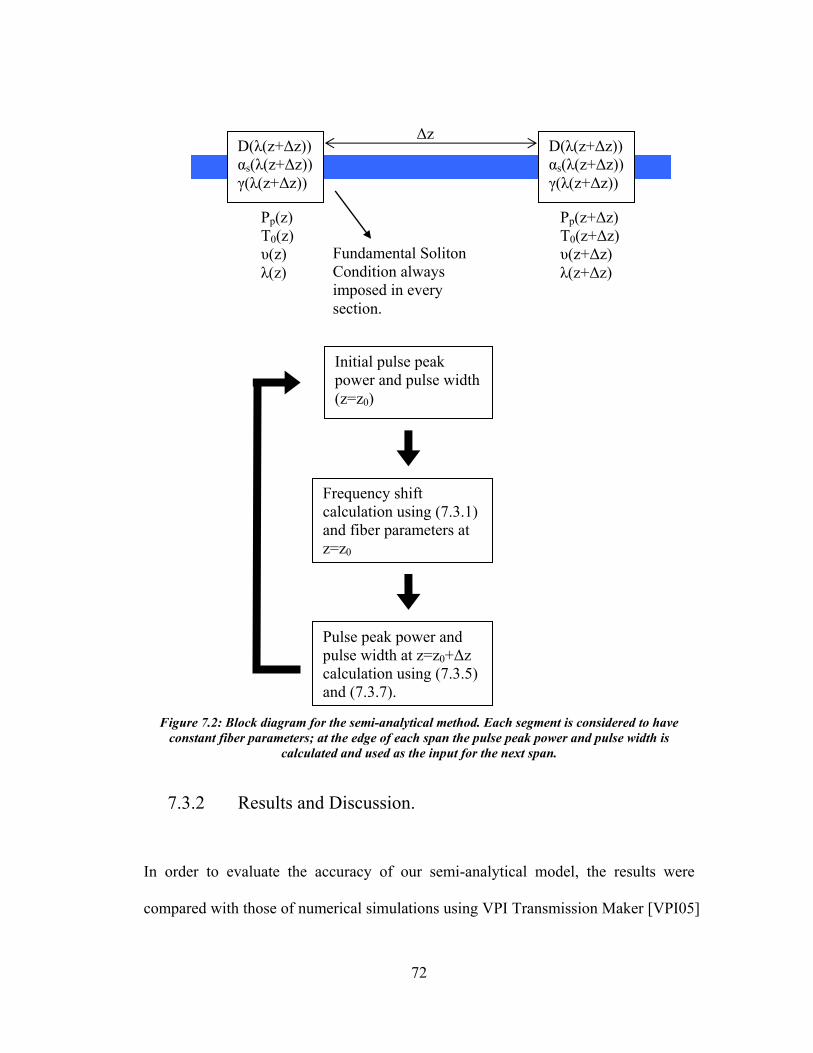
Pp(z) T0(z) υ(z) λ(z)
Pp(z+∆z) T0(z+∆z) υ(z+∆z) λ(z+∆z)
∆z D(λ(z+∆z)) αs(λ(z+∆z)) γ(λ(z+∆z))
D(λ(z+∆z)) αs(λ(z+∆z)) γ(λ(z+∆z))
Fundamental Soliton Condition always imposed in every section.
Initial pulse peak power and pulse width (z=z0)
Frequency shift calculation using (7.3.1) and fiber parameters at z=z0
Pulse peak power and pulse width at z=z0+∆z calculation using (7.3.5) and (7.3.7).
Figure 7.2: Block diagram for the semi-analytical method. Each segment is considered to have constant fiber parameters; at the edge of each span the pulse peak power and pulse width is
calculated and used as the input for the next span.
7.3.2 Results and Discussion.
In order to evaluate the accuracy of our semi-analytical model, the results were
compared with those of numerical simulations using VPI Transmission Maker [VPI05]
72

where the split-step Fourier method was used. Two fibers were used, a polarization
maintaining fiber (PMF) and a HNL-PCF. All the fiber parameters are shown in
Appendix A and the numerical parameters in Appendix B.
In the first case, we consider 100m of PMF (3M FS-PM-7811) as used in [Nor99].
The wavelength of the input soliton pulse is set at 1550nm. Soliton frequency shift
versus input optical pulse width is shown in Fig.7.3, in which, results of semi-
analytical calculation represented by triangles agree well with those obtained by
numerical simulations represented by open circles. The figure also shows the
evolution of the exponent x that relates the SSFS and the pulse width as:
xT −∝∆ 0υ (7.3.8)
In equation (7.1.21) x was 4, representing the fourth power rule. This is verified for
pulses wider than 100fsec, which agrees with the experimental work of [Mit86] where
pulses wider than 420fsec were used.
73

6
1.5
2
2.5
3
3.5
4
4.5
10
1
x dv
(GH
z)
20 40 60 80 100 150 10 2
10 3
10 4
10 5
Pulse width (fsec)
Figure 7.3: Frequency shift versus pulse width for a 100m PMF in log scale (left). The stray line represents the analytical result in (7.1.21), triangles represent the complete semi-analytical solution and circles represent the numerical results. The figure also shows the difference on the exponent x
from the analytical value of 4(right).
When the pulse is shifted to a longer wavelength, it is broadened due to the higher
dispersion. This behavior explains the saturation in the frequency shift for narrow
pulses. It needs to be mentioned that when the pulse width is narrower than 20fs, the
nonlinear Schrödinger equation (6.1.5) is no longer accurate because the narrowband
approximation fails [Agr01] which is beyond the scope of this work.
The fiber loss in this case is only 0.26dB, and thus has not an important impact in the
overall behavior.
74

The second fiber tested was a HNL-PCF (Photonic Crystal Fiber NL-18-710) which
parameters are shown in Appendix A.
In Figure 7.4 we show the numerical results of the SSFS as a function of the pulse
width for different fiber lengths. In every case we verify the saturation behavior for
narrow pulses.
20 30 50 80 10010
1
102
103
104
105
Pulse width (fsec)
dv (G
Hz)
0.1m1m5m10m
Figure 7.4: SSFS for a HNL-PCF with different fiber lengths in log scale. For very short fibers (0.1m) the shift is small enough to maintain the linear characteristic; however, for longer fibers we
can see the saturation effect.
In this case, while the pulse propagates through the fiber, we should not only consider
the increase of the chromatic dispersion, but also the decrease of its nonlinear
parameter and the high attenuation. The overall effect is a decrease of the peak power
of the pulse; as the soliton tries to maintain its fundamental relationship as in equation
(7.3.6), the pulse will also be broadened.
75

Figure 7.5 shows the frequency shift versus soliton pulse width in 10m of HNL-PCF
calculated by semi-analytical model (triangles) and numerical simulations (open
circles). The impact of fiber losses in PCF can not be neglected as it can take values
up 200 dB/km. To illustrate this effect, soliton frequency shift calculated without
fiber loss is also plotted in figure 7.5 (squares) for comparison. Similar to what
happened in the polarization maintaining fiber, the exponent x is equal to 4 at a
relatively wide pulse width and is reduced significantly when the pulse width is
narrower than 100fs.
20 40 60 80 100 150 10 1
10 2
10 3
10 4
10 5
10 6
4.
Pulse Width (fsec)
dv (G
Hz)
x
1.
2
2.
3
3.
4
Figure 7.5: Frequency shift and pulse width for a 10m HNL-PCF in log scale (left). The strait line represents the analytical result (7.1.21), squares the semi-analytical solution with no losses,
triangles the complete semi-analytical solution and circles the numerical result. The figure also shows the difference on the exponent x from the analytical value of 4 (right).
If we consider figure 7.4 for a fixed initial pulse width and different fiber lengths
(vertical direction), we can also observed a saturation behavior. Figure 7.6 shows an
76

example of the wavelength shift as a function of the fiber length, for the same HNL-
PCF, for different pulse widths calculated with semi-analytical model (continuous)
and numerical simulations (circles). The results clearly show the saturation in the
frequency shift at long fiber lengths as has been demonstrated experimentally [Nor99].
The discrepancy between the semi-analytical model and the numerical simulation
when the pulse width is narrower than 40fs is attributed to the effect of higher order
dispersion, which is not included in the semi-analytical model. This discrepancy was
not evident in the previous plots as we were using log scale.
0 2 4 6 8 10780
785
790
795
800
805
810
815
Fiber Length (m)
Cen
ter W
avel
engt
h (n
m)
30 fsec40 fsec100fsec
Pulse Width
Figure 7.6: Wavelength shift and fiber length for a PCF for different soliton pulse widths. Circles
represent the numerical data.
77

In all the cases, there is also agreement between the semi-analytical solution and the
numerical solution in both the output peak power and the output pulse width. The
output fundamental order of the soliton from the numerical solution was verified.
As a conclusion for this chapter, the analysis introduced in [Gor86] needs to be
modified when considering large frequency shifts and fiber with no-constant
parameters. The semi-analytical method introduced agrees with the analytical
formulation for relatively wide pulses and with the numerical solution in every case.
This method does not include the effect of the higher order dispersion.
78

Chapter 8: Short Pulsed Lasers Applications for Two Photons Microscopy
Femtosecond pulses lasers serve as a source for fluorescence microscopy. In this
technique, fluorescent dyes are attached to the target molecule (normally a protein) by
covalent labeling strategies. Once attached, the dyes will absorb the incident light at a
particular wavelength and emit photons at a known longer wavelength. Fluorescence
could be used to determinate presence or absence of the specific species, to
determinate concentration, to perform imaging, to study dynamic characteristics, etc.
[Sch01]
A common implementation consists of a one-photon confocal microscope, using a
Ti:Sa pulsed laser as the pulse source. In recent years two-photon microscopy has
emerged as the selected method for fluorescence microscopy in thick tissues and live
animals. The main difficulty in building a two-photon instrument is the cost of the
laser source as well as the expertise needed to maintain a solid-state laser. The
introduction of a high-power fiber laser allows overcoming both limitations.
In this chapter we will first give a short overview to one and two-photon microscopy,
detailing the differences between both methods. Then, we will introduce our
experimental setup and finally show different two-photon images.
79

8.1 One-Photon Confocal Microscopy
In a one-photon confocal microscopy system the excitation from the pulsed laser is
directed into a microscope objective and focused on the sample. This technique gives
a diffraction-limited spot of approximately 0.5 µm in diameter. [Sch01]
Detector pin-holePhoto
detector
Lens
Lens
Focal plane
Beam splitter
Lens
Out of focus
Fluorescently labeled tissue
3-demensional translation stage
Laser source
Figure 8.1: A Scanning Laser Confocal Microscope Setup. The sample is moving in the three dimensions in order to obtain a 3D image. A pin-hole is introduced in front of the detector for
improving the system’s resolution.
80

Figure 8.1 shows a typical setup where the energy from one absorbed photon gives
rise to the generation of one fluorescent photon.
We can identify several problems with confocal microscopy. First, the receiving
signal will include light from structures above and below the focus plane, limiting the
system’s resolution. A common solution to overcome this background is to introduce
a pin-hole near the detector; in this case we have a loss of signal at the receiver and
thus it may be needed to increase the pump power. Nevertheless, the pin-hole will not
help to reject the scattered excitation light from the target volume. In this case very
narrow bandpass filters may be needed as fluorescence and pump signals are close in
frequency domain.
The second problem that we can identify is related to the wavelength range where this
instruments works. Normally used fluorescence dyes (or fluorophores) will absorb in
the UV-Visible region and will emit at longer wavelength. An example of emission
and absorption spectrum for a family of such dyes is shown in Figure 8.2.
81

Figure 8.2: Absorption and emission spectrum of the Alexa-series one-photon fluorescence dyes.
Working in the UV-Visible region has three major problems: first, tissue cells have
very high absorption coefficient at these wavelengths, thus the penetration depth is
reduced and the possibility of photo-damage living cells increases. Second,
fluorophores are easily bleached when excited by a visible light. Finally, it is difficult
to build appropriate optical elements such as lenses and beam splitters [Den90].
8.2 Two Photons Microscopy
The simultaneous absorption of two photons by an atom or molecule in a single event
was first predicted in 1931 [Xu95] and was called Two-Photon Excitation (TPE).
However, it was only recently that two-photon laser scanning fluorescence
microscopy was demonstrated. In this method, the sample is illuminated with light of
a wavelength approximately twice the peak absorption wavelength of the fluorophore
82

in use. For example a dye absorbing at 400nm will be excited by two photons at
800nm.
As TPE is a second-order process, the number of photons absorbed per molecule per
unit of time (Nabs) by means of TPE depends on the square of the incident optical
power ( I(t) ) [Xu95]:
( ) ( ) ( )∫=V
abs trItrCdVtN ,, 2 rrδ (8.1)
Where ( )trC ,r represents the dye concentration and δ the two-photon absorption cross
section. Measuring the two-photon absorption cross section is usually difficult and it
will vary from the one-photon cross section. Consequently, if for example we take the
dyes in Figure 8.2, their two-photon absorption spectrum will not be the same as in
the figure.
When working in TPE, we can neglect the effects of photo-bleaching because the
target volume is very small and only a small number of dyes would be affected.
Taking a large time scale, we can assume that the dye concentration is constant.
Consequently, we can consider that the time and space components of the pump
intensity can be separated as: ( ) ( ) ( )rStItrIrr
0, = , where ( )rSr is unitless. Equation 8.1 can
be rewritten as:
( ) ( ) ( )∫=V
abs rdVStICtNr22
0δ (8.2)
This result can be used to find the time-averaged number of fluorescence photons
[Xu95]:
83

( ) ( )( )
( ) ( )∫><⎥⎥⎦
⎤
⎢⎢⎣
⎡
><
><>=<
V
rdVStICtItI
tF 22022
0
20
21 r
δφη (8.3)
Where the factor 1/2 reflects that two absorbed photons are needed to generate one
fluorescence photon, the term ( )( ) 2
0
20
><
><
tItI is a measure of the second order temporal
coherence of the pump and should be a constant (normally named g), φ is the
fluorescence quantum efficiency of the dye and η2 the efficiency of the measurement
system at the collecting wavelength. The square dependency of the two-photon
absorption on the pump power means that this phenomenon can only occur over a
very small volume around the focus point. Thus, the resolution of the instrument is
improved over the one-photon excitation and there is no need to use a pin-hole at the
receiver.
Another advantage of two-photon based imaging is that biological tissue has
considerable less scattering and absorption in the NIR wavelength. Consequently, the
penetration depth is increased and the probability of photo-damage reduced [Den90].
8.3 Experimental Acquisition of Two-Photon
Images
A classical setup for obtaining a two-photon image will still utilize a pulsed Ti:Sa
laser source. As we mention in this thesis, there are several advantages when using a
fiber based pulsed laser instead.
84

Working in collaboration with Dr. Carey Johnson’s lab, we performed two
experiments. First we obtained two-photon images using a pulsed fiber-laser emitting
at 780nm as the input pump. Then, we obtained a two-photon image shifting the
pump’s central wavelength to 920nm using a Photonic Crystal Fiber as demonstrated
in Chapter 6. In this second experiment, we do not need any filter at the output of the
wavelength shifter as there was not second order soliton generation and the pumping
pulse (after being dispersed by the fiber) was too broad to generate TPE.
The experimental setup is shown in Figure 8.3; when working at 780nm, the 7m PCF
was removed from the optical table. We utilized a Nikon TE2000 microscope with a
100X objective lens and equipped with a 2D piezo-electric scanning stage; the z-
dimension translation was achieved by manually moving the objective lens.
The sample was composed of fluospheres with 24nm of diameter that were doped
with a fluorescence material. The spheres were immobilized in a 3% agarose solution
at a concentration of 5nM. With these small samples, we were able to measure the
diffraction limit of our instrument when we identify a signal of 310nm of 1/e2
diameter.
85

Microscope Nikon TE2000 Source
7m PCF
Fiber Laser IMRA Femtolite Ultra.
Mechanic Translator
Sample
Detector
OSA
3D Scanning 780 nm fiber laser
Old Ti:Sa Laser (white) and New Fiber Laser (on top).
Figure 8.3: Experimental setup for acquiring a two-photon image. The PCF was removed when working of the 780nm region. The pictures shows the fiber-laser used for the experiment (IMRA
Femtolite Ultra) and compares it size with a classical Ti:Sa laser.
In Figure 8.4 we show a two-photon 2D image of a fluosphere taken in the radial
dimension when using the original pump laser at 780nm. Figure 8.5 shows the radial
intensity profile for the same sample. These were the first two-photon images
recorded at the University of Kansas.
Figure 8.6 and 8.7 show the same results but when the pump laser is shifted to a
longer wavelength using the HNL-PCF. There is no previous record available in the
literature of a two-photon image in this wavelength using a fiber laser.
86

Figure 8.4: Two-photon image of a fluosphere using a 780nm pump laser.
Figure 8.5: Radial intensity profile for a fluosphere using a pump laser at 780nm.
87

Figure 8.6: Two-photon image of a fluosphere using a shifted pump laser to 920nm. We can observe one sphere in the middle of the image and an aggregate in the upper right.
44.5
55.5
6
5
5.5
6
6.5
70
10
20
30
40
50
x (µm)y (µm)
Cou
nts
Figure 8.7: Radial intensity profile for the fluosphere at the center of figure 8.6.
88

8.4 Other applications
The optical setup shown in figure 8.3 can be adapted to perform a variety of
fluorescence based experiments that are out of the scope of this work.
First, we consider the two-photon fluorescence correlation spectroscopy (TPFCS). In
this technique, fluorescence fluctuations caused by the diffusion of molecules through
the focal area are detected and analyzed by autocorrelation or cross-correlation
functions. Applications include concentration assays, measurements of mobility,
reaction kinetics, detection of co-localization of proteins and high throughput
screening [Sch01].
Coherent anti-Stokes Raman scattering (CARS) is a nonlinear Raman process in
which two pump beams (at frequencies ωp and ωs respectively) are mixed in a sample
to generate a signal at the anti-Stoke frequency of ωas=2ωp-ωs. By using CARS we
can obtain high-quality three-dimensional images. A normal setup will include two
different (and expensive) pulsed lasers. However, a small change in our setup would
allow performing the experiment with a single pump. This objective represents
several challenges such as the stretch of the pulse spectrum and the synchronization
of the two beams.
89

CONCLUSIONS
In this work we studied the propagation of short optical pulses along a high nonlinear
photonic crystal fiber. We observed and simulated the formation of Raman solitons
and their frequency shift as a function of the fiber length and the input average power.
A wavelength-shifter was built and its experimental spectrum compared with the
numerical simulation results.
A semi-analytical method for the dependency of the soliton self-frequency shift on its
initial pulse width was introduced as a generalization of the fourth power rule
introduced in [Gor86]. The method agrees well with numerical results and behaviors
predicted in the literature. It also agrees with the analytical result in [Gor86] for small
frequency shifts and no fiber losses. This work was submitted for publication and the
resulting paper is shown in Appendix D.
The wavelength-shifter was introduced in a two-photon microscopy setup to obtain
the first two-photon images at the University of Kansas. The central frequency of the
pump laser was then shifted to obtain an image in a different pump wavelength. There
is no evidence in the literature of any previous successful implementation of this last
experiment.
90

As a consequence of the work detailed in this thesis, a NSF proposal was submitted
for the acquisition of a new laser source and microscope to build a permanent two-
photon instrument.
91

FUTURE WORK
Future work related to this master thesis can be focused in two areas. First, the
analytical formulation of the relationship between the pulse-breakup process and the
formed Raman soliton’s peak power. This analysis, in combination with the soliton
self-frequency shift, will allow obtaining an analytical relationship between the
frequency shift and the input pump average power.
In an experimental phase, a new laser source and a permanent setup will allow to
perform two-photon images, even simultaneously acquiring different colors. It will
also permit the realization of TPFCS and CARS analysis. This last technique
represents some technology challenges as pulse spectrum stretching and pulse
synchronization [Che93].
The availability of a width-varying and power-varying laser source would allow the
experimental verification of the semi-analytical method introduced in this work.
92

GLOSSARY
ASE – Amplified Spontaneous Emission
CARS – Coherent anti-Stokes Raman Scattering
CW – Continuous Wave
DNA – Deoxyribose Nucleic Acid
DDF – Dispersion-Decreasing Fiber
EDFA – Erbium Doped Fiber Amplifier
FT – Fourier Transform
FWHW – Full Width Half Width
FWM – Four Wave Mixing
GVD – Group Velocity Dispersion
HNL – High Nonlinear
MDF – Modal Diameter Field
MF – Microstructured Fiber
MM – Multimode
MMF – Multimode Fiber
MOF – Microstructured Optical Fiber
NIR – Near Infrared
NLS – Nonlinear Schrödinger equation.
PC – Photonic Crystal
PCF – Photonic Crystal Fiber
93

PMD – Polarization Mode Dispersion
PMF – Polarization Maintaining Fiber
PPLN – Periodically Poled Lithium-Niobate
PSFS – Pulse Self-Frequency Shift
SBS – Stimulated Brillouin Scattering
SC – Supercontinuum
SMF – Single Mode Fiber
SPM – Self Phase Modulation
SRS – Stimulated Raman Scattering
SSFS – Soliton Self Frequency Shift
TPE – Two-photon Excitation
TPFCS – Two-Photon Fluorescence Spectroscopy
TPLSM – Two-Photon Laser Scanning Microscopy
UV – Ultra-Violet
WDM – Wavelength Division Multiplexing
XPM – Cross-Phase Modulation
94

REFERENCES
[Agr01] Govind P. Agrawal, Nonlinear Fiber Optics, 3rd edition, Academic Press,
2001.
[Agr201] Govind P. Agrawal, Applications of Nonlinear Fiber Optics, Academic
Press, 2001.
[Agr03] Govind P. Agrawal, Yuri S. Krivshar, Optical Solitons, Elsevier Science,
2003.
[Akh92] Sergei A. Akhmanov, Optics of Femtosecond Laser Pulses, AIP, 1992.
[Arb97] M. A. Arbore, M. M. Fejer, M. E. Fermann, A. Hariharan, A. Galvanauskas
and D. Harter, “Frequency Doubling of femtosecond erbium-fiber soliton lasers in
periodically poled lithium niobate”, Opt. Lett. 22 (1997), 13-15.
[Arb97] M.A. Arbore, M.M. Fejer, M.E. Fermann, A. Hariharan, A. Galvanauskas, D.
Harter, “Frequency doubling of femtosecond erbium-fiber soliton lasers in
periodically poled lithium niobate”, Opt. Lett. 22 (1997),13-15.
[Bea87] P. Beaud, W. Hodel, B. Zysset and H. P. Weber, “Ultrashort pulse
propagation, pulse breakup, and fundamental soliton formulation in a single-mode
optical fiber”, IEEE J. Quantum Electron. 23 (1987), 1938-1946.
[Bja03] Anders Bjarklev, Jes Broeng, Araceli Sanchez Bjarklev, Photonic Crystal
Fibres, Kluwer AP, 2003.
[Bus04] K. Busch, S. Lolkes, R B Wehrspohn, H Foll, Photonic Crystals, Wiley VCH,
2004.
95

[Che93] S.V.Chernikov, E.M.Dianov, D.J. Richardson and D. N. Payne, “Soliton
pulse compression in dispersion-decreasing fiber”, Opt. Lett. 18 (1993), 476-478
[Che02] Ju-xin Cheng, Andreas Volkmer, Lewis D. Book and X. Sunney Xie,
“Multiplex Coherent Ant-Stokes Raman Scattering Microspectroscopy and Study of
Lipid Vesicle”, J. Phys. Chem. B 106 (2002), 8493-8498.
[Den90] Winfried Denk, James H. Strickler and Watt W. Webb, “Two-Photon Laser
Scanning Fluorescence Microscopy”, Science. 248 (1990),73-76.
[Egg03] Slusher Eggleton, Nonlinear Photonic Crystals, Springer, 2003
[Fer00] M.E.Fermann, A. Galvanauskas, M. Hofer, “Ultrafast pulse sources based on
multi-mode optical fibers”, Appl. Phys. B 70 (2000), S13-S23.
[Fuo03] M. Fuochi, F. Poli, S. Selleri, A. Cucinotta, and L, Vincetti, “Study of Raman
amplification properties in triangular photonic crystal fibers”, J. Lightware Technol
21 (2003) 2247-2254.
[Gor86] J.P. Gordon, “Theory of the soliton self-frequency shift”, Opt. Lett. 11 (1986)
659-661.
[Gri00] V. S. Grigoryan, R. M. Mu, G. M. Carter and C. R. Menyuk, “Experimental
Demostration of Long-Distance Dispersion-Managed Soliton Propagation at Zero
Average Dispersion”, Photonic Technology Lett. 12 (2000) 45-46.
[Mit86] F.M.Mitschke and L.F.Mollenauer, “Discovery of the soliton self-frequency
shift”, Opt. Lett 11 (1986), 659-661.
[MIT04] MIT Photonic-Bands (MPB), http://ab-initio.mit.edu/mpb.
96

[Mol85] L.F.Mollenauer, R.H. Stolen and M.N. Islam, “Experimental demonstration
of soliton propagation in long fibers: loss compensated by Raman gain”, Opt. Lett. 10
(1985) 229-231.
[Nel97] L.E. Nelson, D.J. Jones, K. Tamura, H.A. Haus, E.P.Ippen, “Ultrashort-
pulse fiber ring lasers”, Appl. Phys. B 65 (1997), 277-294.
[Nor99] Norihito Nishizawa, Ryuyi Okamura, Toshio Goto, “Analysis of Widely
Tunable Femtosecond Soliton Pulse Generation Using Optical Fibers”, J. Appl. Phys.
38 (1999) 4768.
[Nor02] Norihiko Nishizawa, Youta Ito and Toshio Goto, “0.78-0.90-µm Wavelength-
Tunable Femtosecond Soliton Pulse Generation Using Photonic Crystal Fiber”,
Photonic Technology lett. 14 (2002) 986-988.
[Ort02] A. Ortigosa-Blanch, J. C. Knight and P. St. J. Russell, “Pulse breaking and
supercontinuum generation with 200 fs pump pulses in photonic crystal fibers”, JOSA
B 19 (2002), 2567-2572.
[Pau03] H.N. Paulsen, K.M. Hilligsoe, J. Thogersen, S.R. Keiding, J.J. Larsen,
“Coherent anti-Stokes Raman Scaterring microscopy with a photonic crystal fiber
based light source”, Opt Lett. 28 (2003), 1123-1125.
[Por03] K. Porsezian, V.C. Kuriakose (Editors), Optical Solitons, Theoretical and
Experimental Challenges, Springer, 2003.
[Rei02] D.T. Reid, I.G. Cormack, W.J. Wadsworth,J.C. Knight and P.St.J. Russell,
“Soliton Selft-frequency Shift Effect in Photonic Crystal Fibre”, CLEO 2002.
[Rul03] Claude Rulliere, Femtosecond Laser Pulses, 2nd edition, Springer, 2003.
97

[Sch01] P. Schwille and E. Haustein, Fluorescence Correlation Spectroscopy,
available online.
[Sto89] R.H.Stolen, J.P.Gordon, W.J. Tomlinson and H.A. Haus, “Raman response
function of silica-core fibers”, JOSA B 6 (1989) 1159-1166.
[Sto92] R.H. Stolen and W.J.Tomlinson, “Effect of the Raman part of the nonlinear
refractive index on the propagation of ultrashort optical pulses in fibers”, JOSA B 9
(1992), 565-573.
[VPI05] VPI Transmission Maker Users Manual, VPI Photonics
(http://www.vpiphotonics.com), 2005.
[Xu95] Chris Xu and Watt W. Webb, “Measurement of two-photon excitation cross
sections of molecular fluorophores with data from 690 to 1050nm”, JOSA B 13
(1996), 481-491.
[Zys87] B. Zysset, P. Beaud and W. Hodel, “Generation of optical solitons in the
wavelength region 1.37-1.49 µm”, Appl. Phys. Lett. 50 (1987), 1027-1029.
98

APPENDIX A: Optical Fibers Characteristics
• Crystal Fibre NL-18-710
This nonlinear photonic crystal fiber has a zero dispersion wavelength at 710nm.
Figure A.1 shows an axial profile and Table A.1 its main parameters as given by the
manufacturer.
Figure A.1: Crystal Fibre NL-18-710 axial profile (http://www.crystal-fibre.com)
99

λ (nm) D (ps/nm/km) D slope (ps/nm2/km) γ (W-1 km-1) α (dB/km)
710 0 0.58 139 190
600 -142 1.70 171 210
800 68 0.59 122 170
1000 148 0.25 92 130
1550 185 -0.08 49 80
Table A.1: Crystal Fibre NL-18-710 Parameters (http://www.crystal-fibre.com)
Other fiber parameters:
• Core diameter (average): 1.8±0.1µm.
• Pitch (distance between cladding holes): 2.1±0.1 µm
• Air Filling Fraction in the holey region: >90%
• Width of struts holding the core: 70±10 nm
• Diameter of holey region: 21±0.5 µm
• Diameter of outer silica cladding (OD): 125±1 µm
• Coating diameter (single layer acrylate): 230±5 µm
In Figures A.2 through A.4 we plot the wavelength dependency of the fiber´s
parameters.
100

400 600 800 1000 1200 1400 1600 180060
80
100
120
140
160
180
200
220
240
260
Wavelength (nm)
Atte
nuat
ion
(dB
/km
)
400 600 800 1000 1200 1400 1600 18000.04
0.06
0.08
0.1
0.12
0.14
0.16
0.18
0.2
0.22
Wavelength (nm)
Non
linea
r Coe
ffici
ent (
1/W
m)
Figure A.2: Attenuation Parameter (α) for Crystal Fibre NL-18-710. The circles represent the values on Table A.1, the rest of the values were calculated by linear interpolation.
Figure A.3: Nonlinear Coefficient (γ) for a Crystal Fibre NL-18-710. The circles represent the values on Table A.1, the rest of the values were calculated by linear interpolation.
101

400 600 800 1000 1200 1400 1600 1800-400
-300
-200
-100
0
100
200
Wavelength (nm)
Dis
pers
ion
(pse
c/nm
km
)
Figure A.4: Dispersion Coefficient (D) for a Crystal Fibre NL-18-710. The circles represent the values on Table A.1, the rest of the values were calculated by linear interpolation.
• 3M FS-PM-7811
This is a polarization-maintaining fiber with a small core area in order to achieve a
large nonlinear index.
The fiber parameters are:
• Operating Wavelength: 1550nm.
• Mode Field Diameter: 5.5 µm.
• Dispersion parameter: 1.177 s/m2.
• Dispersion slope at 1550nm: 80 s/m3.
102

• Dispersion Law: ( )75 1055.110877.11 −− ×−×+= λD in [ps/nm2], where λ is in [cm].
• Nonlinear Parameter: ( )110044.0 −− ⋅= mWγ .
• Attenuation Typical at 1550nm: kmdB /6.2=α .
• Birefringence: . 4107 −×
103

APPENDIX B: VPI Models and Numerical Parameters
The numerical simulations in this Thesis were performed using the software VPI
Transmission Maker [VPI05]. It is a graphical programming software that includes an
important library of optical components. In our study we just needed to model
different pulses propagation through different fibers, so the simulation model was
very simple. The simulation model is shown in Figure B.1 and the principal
numerical parameters in Table B.1.
Figure B.1: VPI Model used for simulations.
104

Parameter Value
Time Windows 40ps (*)
Frequency Bandwidth 204.8 THz
Bit Rate Default 1/40 x 1012 bps
Table B.1: Numerical Parameters.
(*) for very small frequency shifts, this value was increased to 80ps or 160ps.
The parameters’ values in an xml format are shown next for each type of fiber.
1) Photonic Crystal Fiber Simulation Parameters:
i. Global Parameters:
<?xml version='1.0' encoding='UTF-8' ?> <!DOCTYPE SAVEDSTATES> <SAVEDSTATES master="PhotonicCrystalFiberThesis.vtmu"> <STATEVALUE unit="s" category="Global" label="TimeWindow" value="4e-11" __key="value" type="float"></STATEVALUE> <STATEVALUE unit="" category="Global" label="InBandNoiseBins" value="OFF" __key="value" type="enumeration"></STATEVALUE> <STATEVALUE unit="" category="Global" label="BoundaryConditions" value="Periodic" __key="value" type="enumeration"></STATEVALUE> <STATEVALUE unit="" category="Global" label="LogicalInformation" value="ON" __key="value" type="enumeration"></STATEVALUE> <STATEVALUE unit="Hz" category="Global" label="SampleModeBandwidth" value="204.8e12" __key="value" type="float"></STATEVALUE> <STATEVALUE unit="Hz" category="Global" label="SampleModeCenterFrequency" value="384.615e12" __key="value" type="float"></STATEVALUE> <STATEVALUE unit="Hz" category="Global" label="SampleRateDefault" value="204.8e12" __key="value" type="float"></STATEVALUE> <STATEVALUE unit="bit/s" category="Global" label="BitRateDefault" value="1/4e-11" __key="value" type="float"></STATEVALUE> <STATEVALUE unit="Hz" category="PulsedLaser" label="PulseCenterFrequency" value="384.615e12" __key="value" type="float"></STATEVALUE> <STATEVALUE unit="W" category="PulsedLaser" label="AveragePower" value="5e-3" __key="value" type="float"></STATEVALUE> <STATEVALUE unit="Hz" category="PulsedLaser" label="RepeatitionRate" value="50e6" __key="value" type="float"></STATEVALUE>
105

<STATEVALUE unit="s" category="PulsedLaser" label="To" value="100e-15" __key="value" type="float"></STATEVALUE> </SAVEDSTATES>
ii. Fiber Parameters:
<?xml version='1.0' encoding='UTF-8' ?> <!DOCTYPE SAVEDSTATES> <SAVEDSTATES master="UniversalFiberFwd.vtmg"> <STATEVALUE unit="" category="Physical" label="NumberOfFiberSpans" value="1" __key="value" type="int"></STATEVALUE> <STATEVALUE unit="m" category="Physical" label="Length" value="0.1" __key="value" type="floatarray"></STATEVALUE> <STATEVALUE unit="" category="Physical" label="AttenuationDescription" value="AttenuationFile" __key="value" type="enumeration"></STATEVALUE> <STATEVALUE unit="dB/m" category="Physical" label="Attenuation" value="0.2e-3" __key="value" type="floatarray"></STATEVALUE> <STATEVALUE unit="" category="Physical" label="AttFilename" value="Attenuation710.txt" __key="value" type="inputfilearray"></STATEVALUE> <STATEVALUE unit="Hz" category="Physical" label="ReferenceFrequency" value="PulseCenterFrequency" __key="value" type="float"></STATEVALUE> <STATEVALUE unit="" category="Physical" label="DispersionDescription" value="DispersionFile" __key="value" type="enumeration"></STATEVALUE> <STATEVALUE unit="s/m^2" category="Physical" label="Dispersion" value="16e-6" __key="value" type="floatarray"></STATEVALUE> <STATEVALUE unit="s/m^3" category="Physical" label="DispersionSlope" value="0.08e3" __key="value" type="floatarray"></STATEVALUE> <STATEVALUE unit="" category="Physical" label="DispersionFilename" value="Dispersion710.txt" __key="value" type="inputfilearray"></STATEVALUE> <STATEVALUE unit="" category="Physical" label="RamanScattering" value="Yes" __key="value" type="enumeration"></STATEVALUE> <STATEVALUE unit="" category="Physical" label="RamanFilename" value="RamanNew.txt" __key="value" type="inputfilearray"></STATEVALUE> <STATEVALUE unit="" category="Physical" label="RamanAdjustmentFactors" value="0.5" __key="value" type="floatarray"></STATEVALUE> <STATEVALUE unit="" category="Physical" label="SpontaneousRamanScattering" value="No" __key="value" type="enumeration"></STATEVALUE> <STATEVALUE unit="" category="Physical" label="RamanFraction" value="0.17" __key="value" type="floatarray"></STATEVALUE> <STATEVALUE unit="K" category="Physical" label="Temperature" value="300.0" __key="value" type="floatarray"></STATEVALUE> <STATEVALUE unit="s/(m^1/2)" category="Physical" label="PMDCoefficient" value="0.1e-12/31.62" __key="value" type="float"></STATEVALUE> <STATEVALUE unit="m" category="Physical" label="CorrelationLength"
106

value="50.0" __key="value" type="float"></STATEVALUE> <STATEVALUE unit="" category="Physical" label="NonlinearDescription" value="NonlinearFile" __key="value" type="enumeration"></STATEVALUE> <STATEVALUE unit="m^2/W" category="Physical" label="NonLinearIndex" value="8.2e-19" __key="value" type="floatarray"></STATEVALUE> <STATEVALUE unit="" category="Physical" label="NonLinearFilename" value="NonLinear710.txt" __key="value" type="inputfilearray"></STATEVALUE> <STATEVALUE unit="" category="Physical" label="CoreAreaDescription" value="CoreAreaParameter" __key="value" type="enumeration"></STATEVALUE> <STATEVALUE unit="m^2" category="Physical" label="CoreArea" value="1.77e-12" __key="value" type="floatarray"></STATEVALUE> <STATEVALUE unit="" category="Physical" label="CoreAreaFilename" value="" __key="value" type="inputfilearray"></STATEVALUE> <STATEVALUE unit="" category="Physical" label="OverlapIntegralFilename" value="" __key="value" type="inputfilearray"></STATEVALUE> <STATEVALUE unit="" category="Physical" label="EventLossDescription" value="EventLossParameter" __key="value" type="enumeration"></STATEVALUE> <STATEVALUE unit="dB" category="Physical" label="EventLoss" value="0.0" __key="value" type="floatarray"></STATEVALUE> <STATEVALUE unit="" category="Physical" label="EventLossFilename" value="" __key="value" type="inputfilearray"></STATEVALUE> <STATEVALUE unit="Hz" category="Numerical" label="FreqResolutionNB" value="25e9" __key="value" type="float"></STATEVALUE> <STATEVALUE unit="Hz" category="Numerical" label="FreqResolutionSFB" value="25e9" __key="value" type="float"></STATEVALUE> <STATEVALUE unit="Hz" category="Numerical" label="GridReferenceFrequency" value="PulseCenterFrequency" __key="value" type="float"></STATEVALUE> <STATEVALUE unit="" category="Numerical" label="SpectralDiscretizerDescription" value="FixedFrequencies" __key="value" type="enumeration"></STATEVALUE> <STATEVALUE unit="Hz" category="Numerical" label="NoiseCenterFrequency" value="PulseCenterFrequency" __key="value" type="float"></STATEVALUE> <STATEVALUE unit="Hz" category="Numerical" label="NoiseBandwidth" value="10e12" __key="value" type="float"></STATEVALUE> <STATEVALUE unit="dB" category="Numerical" label="AccuracyGoal" value="0.01" __key="value" type="float"></STATEVALUE> <STATEVALUE unit="" category="Numerical" label="IterationAccuracyFactor" value="10.0" __key="value" type="float"></STATEVALUE> <STATEVALUE unit="m" category="Numerical" label="InitialStepSize" value="0.01" __key="value" type="floatarray"></STATEVALUE> <STATEVALUE unit="m" category="Numerical" label="MinimumStepSize" value="0.005" __key="value" type="float"></STATEVALUE> <STATEVALUE unit="" category="Numerical" label="SplitStepType" value="Symmetric" __key="value" type="enumeration"></STATEVALUE> <STATEVALUE unit="m" category="Numerical" label="MaxStepWidth" value=".1" __key="value" type="float"></STATEVALUE> <STATEVALUE unit="deg" category="Numerical" label="MaxPhaseChange"
107

value="0.5" __key="value" type="float"></STATEVALUE> <STATEVALUE unit="m" category="Numerical" label="MeanStepWidth" value="1.0e3" __key="value" type="float"></STATEVALUE> <STATEVALUE unit="m" category="Numerical" label="WidthDeviation" value="100.0" __key="value" type="float"></STATEVALUE> <STATEVALUE unit="" category="Enhanced" label="PolarizationAnalysis" value="Scalar" __key="value" type="enumeration"></STATEVALUE> <STATEVALUE unit="" category="Enhanced" label="NoisePolarization" value="Unpolarized" __key="value" type="enumeration"></STATEVALUE> <STATEVALUE unit="" category="Enhanced" label="DistortionPolarization" value="Unpolarized" __key="value" type="enumeration"></STATEVALUE> <STATEVALUE unit="" category="Enhanced" label="NonlinearAdjustmentFactors" value="1.0 1.0 1.0 1.0 0.5" __key="value" type="floatarray"></STATEVALUE> <STATEVALUE unit="" category="Enhanced" label="WidthRandomNumberSeed" value="0" __key="value" type="int"></STATEVALUE> <STATEVALUE unit="" category="Enhanced" label="ScatteringRandomNumberSeed" value="0" __key="value" type="int"></STATEVALUE> <STATEVALUE unit="" category="Enhanced" label="FreezeWidth" value="0" __key="value" type="int"></STATEVALUE> <STATEVALUE unit="" category="Enhanced" label="FreezeScattering" value="0" __key="value" type="int"></STATEVALUE> <STATEVALUE unit="" category="Enhanced" label="CorrelationScatteringFactor" value="0.0" __key="value" type="float"></STATEVALUE> <STATEVALUE unit="" category="Enhanced" label="BirefringenceProfile" value="None" __key="value" type="enumeration"></STATEVALUE> <STATEVALUE unit="" category="Enhanced" label="BirefringenceFileDataType" value="RotationMatrices" __key="value" type="enumeration"></STATEVALUE> <STATEVALUE unit="" category="Enhanced" label="BirefringenceInputFilename" value="" __key="value" type="inputfile"></STATEVALUE> <STATEVALUE unit="" category="Enhanced" label="BirefringenceOutputFilename" value="" __key="value" type="outputfile"></STATEVALUE> <STATEVALUE unit="" category="Enhanced" label="LikelihoodRatiosFilename" value="" __key="value" type="outputfile"></STATEVALUE> <STATEVALUE unit="" category="Enhanced" label="FieldAnalysis" value="Yes" __key="value" type="enumeration"></STATEVALUE> <STATEVALUE unit="" category="Enhanced" label="SkipFieldAnalysis" value="0" __key="value" type="int"></STATEVALUE> <STATEVALUE unit="" category="Enhanced" label="SPM_EC" value="Yes" __key="value" type="enumeration"></STATEVALUE> <STATEVALUE unit="" category="Enhanced" label="XPM_EC" value="Yes" __key="value" type="enumeration"></STATEVALUE> <STATEVALUE unit="" category="Enhanced" label="XPM_MC" value="Yes" __key="value" type="enumeration"></STATEVALUE> <STATEVALUE unit="" category="Enhanced" label="IntraBandRaman" value="Yes" __key="value" type="enumeration"></STATEVALUE> <STATEVALUE unit="" category="Enhanced" label="InterBandRaman"
108

value="Yes" __key="value" type="enumeration"></STATEVALUE> <STATEVALUE unit="" category="Enhanced" label="HigherOrderNLEffects" value="Yes" __key="value" type="enumeration"></STATEVALUE> <STATEVALUE unit="" category="Enhanced" label="NoiseBinInteractions" value="Yes" __key="value" type="enumeration"></STATEVALUE> <STATEVALUE unit="" category="Enhanced" label="DistortionInteractions" value="Yes" __key="value" type="enumeration"></STATEVALUE> <STATEVALUE unit="" category="Enhanced" label="Options" value="" __key="value" type="string"></STATEVALUE> <STATEVALUE unit="" category="Enhanced" label="PowerPlotPoints" value="101" __key="value" type="int"></STATEVALUE> <STATEVALUE unit="" category="Enhanced" label="LogFilename" value="" __key="value" type="outputfile"></STATEVALUE> <STATEVALUE unit="" category="Enhanced" label="ConserveMemory" value="No" __key="value" type="enumeration"></STATEVALUE> <STATEVALUE unit="" category="Enhanced" label="NoiseRandomNumberSeed" value="0" __key="value" type="int"></STATEVALUE> <STATEVALUE unit="" category="Enhanced" label="Active" value="On" __key="value" type="enumeration"></STATEVALUE> </SAVEDSTATES>
iii. Pulse Parameter:
<?xml version='1.0' encoding='UTF-8' ?> <!DOCTYPE SAVEDSTATES> <SAVEDSTATES master="TxPulseSechOpt.vtmg"> <STATEVALUE unit="Hz" category="Physical" label="SampleRate" value="SampleRateDefault" __key="value" type="float"></STATEVALUE> <STATEVALUE unit="bit/s" category="Physical" label="BitRate" value="BitRateDefault" __key="value" type="float"></STATEVALUE> <STATEVALUE unit="Hz" category="Physical" label="EmissionFrequency" value="PulseCenterFrequency" __key="value" type="float"></STATEVALUE> <STATEVALUE unit="W" category="Physical" label="PeakPower" value="! " expr AveragePower / (RepeatitionRate * To)"" __key="value" type="float"></STATEVALUE> <STATEVALUE unit="s" category="Physical" label="FWHM" value="!" expr To*2* sqrt( log(2) )"" __key="value" type="float"></STATEVALUE> <STATEVALUE unit="" category="Physical" label="CenterPosition" value="0.5" __key="value" type="float"></STATEVALUE> <STATEVALUE unit="deg" category="Physical" label="InitialPhase" value="0.0" __key="value" type="float"></STATEVALUE> <STATEVALUE unit="deg" category="Physical" label="Azimuth" value="0" __key="value" type="float"></STATEVALUE> <STATEVALUE unit="deg" category="Physical" label="Ellipticity" value="0" __key="value" type="float"></STATEVALUE> <STATEVALUE unit="" category="Physical" label="PreSpaces" value="0"
109

__key="value" type="int"></STATEVALUE> <STATEVALUE unit="" category="Physical" label="PostSpaces" value="0" __key="value" type="int"></STATEVALUE> <STATEVALUE unit="" category="Physical" label="PRBS_Type" value="PRBS" __key="value" type="enumeration"></STATEVALUE> <STATEVALUE unit="" category="Physical" label="MarkProbability" value="0.5" __key="value" type="float"></STATEVALUE> <STATEVALUE unit="" category="Physical" label="PRBS_Order" value="7" __key="value" type="int"></STATEVALUE> <STATEVALUE unit="" category="Physical" label="MarkNumber" value="7" __key="value" type="int"></STATEVALUE> <STATEVALUE unit="" category="Physical" label="CodeWord" value="" __key="value" type="intarray"></STATEVALUE> <STATEVALUE unit="" category="Physical" label="InputFilename" value="" __key="value" type="inputfile"></STATEVALUE> <STATEVALUE unit="" category="Numerical" label="ExcessPulseSlots" value="3" __key="value" type="int"></STATEVALUE> <STATEVALUE unit="" category="Enhanced" label="RandomNumberSeed" value="0" __key="value" type="int"></STATEVALUE> <STATEVALUE unit="" category="Enhanced" label="OutputFilename" value="" __key="value" type="outputfile"></STATEVALUE> <STATEVALUE unit="" category="Enhanced" label="ControlFlagReset" value="Continue" __key="value" type="enumeration"></STATEVALUE> <STATEVALUE unit="" category="Enhanced" label="ControlFlagWrite" value="Overwrite" __key="value" type="enumeration"></STATEVALUE> <STATEVALUE unit="" category="Enhanced" label="OutputDataType" value="Blocks" __key="value" type="enumeration"></STATEVALUE> <STATEVALUE unit="" category="Enhanced" label="ChannelLabel" value="" __key="value" type="string"></STATEVALUE> </SAVEDSTATES>
2) Polarization maintaining fiber parameters:
i. Global Parameters:
<?xml version='1.0' encoding='UTF-8' ?> <!DOCTYPE SAVEDSTATES> <SAVEDSTATES master="PhotonicCrystalFiber31.vtmu"> <STATEVALUE unit="s" category="Global" label="TimeWindow" value="80e-12" __key="value" type="float"></STATEVALUE> <STATEVALUE unit="" category="Global" label="InBandNoiseBins" value="OFF" __key="value" type="enumeration"></STATEVALUE> <STATEVALUE unit="" category="Global" label="BoundaryConditions" value="Periodic" __key="value" type="enumeration"></STATEVALUE> <STATEVALUE unit="" category="Global" label="LogicalInformation" value="ON" __key="value" type="enumeration"></STATEVALUE> <STATEVALUE unit="Hz" category="Global" label="SampleModeBandwidth"
110

value="204.8e12" __key="value" type="float"></STATEVALUE> <STATEVALUE unit="Hz" category="Global" label="SampleModeCenterFrequency" value="193.1e12" __key="value" type="float"></STATEVALUE> <STATEVALUE unit="Hz" category="Global" label="SampleRateDefault" value="204.8e12" __key="value" type="float"></STATEVALUE> <STATEVALUE unit="bit/s" category="Global" label="BitRateDefault" value="1/80e-12" __key="value" type="float"></STATEVALUE> <STATEVALUE unit="Hz" category="PulsedLaser" label="PulseCenterFrequency" value="193.1e12" __key="value" type="float"></STATEVALUE> <STATEVALUE unit="W" category="PulsedLaser" label="AveragePower" value="5.5e-3" __key="value" type="float"></STATEVALUE> <STATEVALUE unit="Hz" category="PulsedLaser" label="RepeatitionRate" value="48e6" __key="value" type="float"></STATEVALUE> <STATEVALUE unit="s" category="PulsedLaser" label="To" value="100e-15" __key="value" type="float"></STATEVALUE> </SAVEDSTATES>
ii. Fiber Parameters:
<?xml version='1.0' encoding='UTF-8' ?> <!DOCTYPE SAVEDSTATES> <SAVEDSTATES master="UniversalFiberFwd.vtmg"> <STATEVALUE unit="" category="Physical" label="NumberOfFiberSpans" value="1" __key="value" type="int"></STATEVALUE> <STATEVALUE unit="m" category="Physical" label="Length" value="0.1" __key="value" type="floatarray"></STATEVALUE> <STATEVALUE unit="" category="Physical" label="AttenuationDescription" value="AttenuationParameter" __key="value" type="enumeration"></STATEVALUE> <STATEVALUE unit="dB/m" category="Physical" label="Attenuation" value="2.6e-3" __key="value" type="floatarray"></STATEVALUE> <STATEVALUE unit="" category="Physical" label="AttFilename" value="AttenuationL01.txt" __key="value" type="inputfilearray"></STATEVALUE> <STATEVALUE unit="Hz" category="Physical" label="ReferenceFrequency" value="PulseCenterFrequency" __key="value" type="float"></STATEVALUE> <STATEVALUE unit="" category="Physical" label="DispersionDescription" value="DispersionParameters" __key="value" type="enumeration"></STATEVALUE> <STATEVALUE unit="s/m^2" category="Physical" label="Dispersion" value="1.177e-5" __key="value" type="floatarray"></STATEVALUE> <STATEVALUE unit="s/m^3" category="Physical" label="DispersionSlope" value="0.08e3" __key="value" type="floatarray"></STATEVALUE> <STATEVALUE unit="" category="Physical" label="DispersionFilename" value="DispersionL01.txt" __key="value" type="inputfilearray"></STATEVALUE> <STATEVALUE unit="" category="Physical" label="RamanScattering" value="Yes" __key="value" type="enumeration"></STATEVALUE> <STATEVALUE unit="" category="Physical" label="RamanFilename"
111

value=""$BNROOT/data/UFM/RamanGain.dat"" __key="value" type="inputfilearray"></STATEVALUE> <STATEVALUE unit="" category="Physical" label="RamanAdjustmentFactors" value="0.5" __key="value" type="floatarray"></STATEVALUE> <STATEVALUE unit="" category="Physical" label="SpontaneousRamanScattering" value="No" __key="value" type="enumeration"></STATEVALUE> <STATEVALUE unit="" category="Physical" label="RamanFraction" value="0.17" __key="value" type="floatarray"></STATEVALUE> <STATEVALUE unit="K" category="Physical" label="Temperature" value="300.0" __key="value" type="floatarray"></STATEVALUE> <STATEVALUE unit="s/(m^1/2)" category="Physical" label="PMDCoefficient" value="0.1e-12/31.62" __key="value" type="float"></STATEVALUE> <STATEVALUE unit="m" category="Physical" label="CorrelationLength" value="50.0" __key="value" type="float"></STATEVALUE> <STATEVALUE unit="" category="Physical" label="NonlinearDescription" value="NonlinearIndexParameter" __key="value" type="enumeration"></STATEVALUE> <STATEVALUE unit="m^2/W" category="Physical" label="NonLinearIndex" value="2.6e-20" __key="value" type="floatarray"></STATEVALUE> <STATEVALUE unit="" category="Physical" label="NonLinearFilename" value="NonLinearL01.txt" __key="value" type="inputfilearray"></STATEVALUE> <STATEVALUE unit="" category="Physical" label="CoreAreaDescription" value="CoreAreaParameter" __key="value" type="enumeration"></STATEVALUE> <STATEVALUE unit="m^2" category="Physical" label="CoreArea" value="23.76e-12" __key="value" type="floatarray"></STATEVALUE> <STATEVALUE unit="" category="Physical" label="CoreAreaFilename" value="Area710.txt" __key="value" type="inputfilearray"></STATEVALUE> <STATEVALUE unit="" category="Physical" label="OverlapIntegralFilename" value="" __key="value" type="inputfilearray"></STATEVALUE> <STATEVALUE unit="" category="Physical" label="EventLossDescription" value="EventLossParameter" __key="value" type="enumeration"></STATEVALUE> <STATEVALUE unit="dB" category="Physical" label="EventLoss" value="0.0" __key="value" type="floatarray"></STATEVALUE> <STATEVALUE unit="" category="Physical" label="EventLossFilename" value="" __key="value" type="inputfilearray"></STATEVALUE> <STATEVALUE unit="Hz" category="Numerical" label="FreqResolutionNB" value="100e9" __key="value" type="float"></STATEVALUE> <STATEVALUE unit="Hz" category="Numerical" label="FreqResolutionSFB" value="100e9" __key="value" type="float"></STATEVALUE> <STATEVALUE unit="Hz" category="Numerical" label="GridReferenceFrequency" value="PulseCenterFrequency" __key="value" type="float"></STATEVALUE> <STATEVALUE unit="" category="Numerical" label="SpectralDiscretizerDescription" value="FixedFrequencies" __key="value" type="enumeration"></STATEVALUE> <STATEVALUE unit="Hz" category="Numerical" label="NoiseCenterFrequency" value="193.1e12" __key="value"
112

type="float"></STATEVALUE> <STATEVALUE unit="Hz" category="Numerical" label="NoiseBandwidth" value="10e12" __key="value" type="float"></STATEVALUE> <STATEVALUE unit="dB" category="Numerical" label="AccuracyGoal" value="0.01" __key="value" type="float"></STATEVALUE> <STATEVALUE unit="" category="Numerical" label="IterationAccuracyFactor" value="10.0" __key="value" type="float"></STATEVALUE> <STATEVALUE unit="m" category="Numerical" label="InitialStepSize" value="1000.0" __key="value" type="floatarray"></STATEVALUE> <STATEVALUE unit="m" category="Numerical" label="MinimumStepSize" value="1.0" __key="value" type="float"></STATEVALUE> <STATEVALUE unit="" category="Numerical" label="SplitStepType" value="Symmetric" __key="value" type="enumeration"></STATEVALUE> <STATEVALUE unit="m" category="Numerical" label="MaxStepWidth" value="1.0e3" __key="value" type="float"></STATEVALUE> <STATEVALUE unit="deg" category="Numerical" label="MaxPhaseChange" value="0.05" __key="value" type="float"></STATEVALUE> <STATEVALUE unit="m" category="Numerical" label="MeanStepWidth" value="1.0e3" __key="value" type="float"></STATEVALUE> <STATEVALUE unit="m" category="Numerical" label="WidthDeviation" value="100.0" __key="value" type="float"></STATEVALUE> <STATEVALUE unit="" category="Enhanced" label="PolarizationAnalysis" value="Scalar" __key="value" type="enumeration"></STATEVALUE> <STATEVALUE unit="" category="Enhanced" label="NoisePolarization" value="Unpolarized" __key="value" type="enumeration"></STATEVALUE> <STATEVALUE unit="" category="Enhanced" label="DistortionPolarization" value="Unpolarized" __key="value" type="enumeration"></STATEVALUE> <STATEVALUE unit="" category="Enhanced" label="NonlinearAdjustmentFactors" value="1.0 1.0 1.0 1.0 0.5" __key="value" type="floatarray"></STATEVALUE> <STATEVALUE unit="" category="Enhanced" label="WidthRandomNumberSeed" value="0" __key="value" type="int"></STATEVALUE> <STATEVALUE unit="" category="Enhanced" label="ScatteringRandomNumberSeed" value="0" __key="value" type="int"></STATEVALUE> <STATEVALUE unit="" category="Enhanced" label="FreezeWidth" value="0" __key="value" type="int"></STATEVALUE> <STATEVALUE unit="" category="Enhanced" label="FreezeScattering" value="0" __key="value" type="int"></STATEVALUE> <STATEVALUE unit="" category="Enhanced" label="CorrelationScatteringFactor" value="0.0" __key="value" type="float"></STATEVALUE> <STATEVALUE unit="" category="Enhanced" label="BirefringenceProfile" value="None" __key="value" type="enumeration"></STATEVALUE> <STATEVALUE unit="" category="Enhanced" label="BirefringenceFileDataType" value="RotationMatrices" __key="value" type="enumeration"></STATEVALUE> <STATEVALUE unit="" category="Enhanced" label="BirefringenceInputFilename" value="" __key="value" type="inputfile"></STATEVALUE> <STATEVALUE unit="" category="Enhanced" label="BirefringenceOutputFilename" value="" __key="value"
113

type="outputfile"></STATEVALUE> <STATEVALUE unit="" category="Enhanced" label="LikelihoodRatiosFilename" value="" __key="value" type="outputfile"></STATEVALUE> <STATEVALUE unit="" category="Enhanced" label="FieldAnalysis" value="Yes" __key="value" type="enumeration"></STATEVALUE> <STATEVALUE unit="" category="Enhanced" label="SkipFieldAnalysis" value="0" __key="value" type="int"></STATEVALUE> <STATEVALUE unit="" category="Enhanced" label="SPM_EC" value="Yes" __key="value" type="enumeration"></STATEVALUE> <STATEVALUE unit="" category="Enhanced" label="XPM_EC" value="Yes" __key="value" type="enumeration"></STATEVALUE> <STATEVALUE unit="" category="Enhanced" label="XPM_MC" value="Yes" __key="value" type="enumeration"></STATEVALUE> <STATEVALUE unit="" category="Enhanced" label="IntraBandRaman" value="Yes" __key="value" type="enumeration"></STATEVALUE> <STATEVALUE unit="" category="Enhanced" label="InterBandRaman" value="Yes" __key="value" type="enumeration"></STATEVALUE> <STATEVALUE unit="" category="Enhanced" label="HigherOrderNLEffects" value="No" __key="value" type="enumeration"></STATEVALUE> <STATEVALUE unit="" category="Enhanced" label="NoiseBinInteractions" value="Yes" __key="value" type="enumeration"></STATEVALUE> <STATEVALUE unit="" category="Enhanced" label="DistortionInteractions" value="Yes" __key="value" type="enumeration"></STATEVALUE> <STATEVALUE unit="" category="Enhanced" label="Options" value="" __key="value" type="string"></STATEVALUE> <STATEVALUE unit="" category="Enhanced" label="PowerPlotPoints" value="101" __key="value" type="int"></STATEVALUE> <STATEVALUE unit="" category="Enhanced" label="LogFilename" value="" __key="value" type="outputfile"></STATEVALUE> <STATEVALUE unit="" category="Enhanced" label="ConserveMemory" value="No" __key="value" type="enumeration"></STATEVALUE> <STATEVALUE unit="" category="Enhanced" label="NoiseRandomNumberSeed" value="0" __key="value" type="int"></STATEVALUE> <STATEVALUE unit="" category="Enhanced" label="Active" value="On" __key="value" type="enumeration"></STATEVALUE> </SAVEDSTATES>
iii. Pulse Parameters:
<?xml version='1.0' encoding='UTF-8' ?> <!DOCTYPE SAVEDSTATES> <SAVEDSTATES master="TxPulseSechOpt.vtmg"> <STATEVALUE unit="Hz" category="Physical" label="SampleRate" value="SampleRateDefault" __key="value" type="float"></STATEVALUE> <STATEVALUE unit="bit/s" category="Physical" label="BitRate" value="BitRateDefault" __key="value" type="float"></STATEVALUE> <STATEVALUE unit="Hz" category="Physical" label="EmissionFrequency" value="PulseCenterFrequency" __key="value" type="float"></STATEVALUE> <STATEVALUE unit="W" category="Physical" label="PeakPower"
114

value="!" expr AveragePower/(RepeatitionRate*To)"" __key="value" type="float"></STATEVALUE> <STATEVALUE unit="s" category="Physical" label="FWHM" value="!" expr To*2* sqrt( log(2) )"" __key="value" type="float"></STATEVALUE> <STATEVALUE unit="" category="Physical" label="CenterPosition" value="0.5" __key="value" type="float"></STATEVALUE> <STATEVALUE unit="deg" category="Physical" label="InitialPhase" value="0.0" __key="value" type="float"></STATEVALUE> <STATEVALUE unit="deg" category="Physical" label="Azimuth" value="0" __key="value" type="float"></STATEVALUE> <STATEVALUE unit="deg" category="Physical" label="Ellipticity" value="0" __key="value" type="float"></STATEVALUE> <STATEVALUE unit="" category="Physical" label="PreSpaces" value="0" __key="value" type="int"></STATEVALUE> <STATEVALUE unit="" category="Physical" label="PostSpaces" value="0" __key="value" type="int"></STATEVALUE> <STATEVALUE unit="" category="Physical" label="PRBS_Type" value="PRBS" __key="value" type="enumeration"></STATEVALUE> <STATEVALUE unit="" category="Physical" label="MarkProbability" value="0.5" __key="value" type="float"></STATEVALUE> <STATEVALUE unit="" category="Physical" label="PRBS_Order" value="7" __key="value" type="int"></STATEVALUE> <STATEVALUE unit="" category="Physical" label="MarkNumber" value="7" __key="value" type="int"></STATEVALUE> <STATEVALUE unit="" category="Physical" label="CodeWord" value="" __key="value" type="intarray"></STATEVALUE> <STATEVALUE unit="" category="Physical" label="InputFilename" value="" __key="value" type="inputfile"></STATEVALUE> <STATEVALUE unit="" category="Numerical" label="ExcessPulseSlots" value="3" __key="value" type="int"></STATEVALUE> <STATEVALUE unit="" category="Enhanced" label="RandomNumberSeed" value="0" __key="value" type="int"></STATEVALUE> <STATEVALUE unit="" category="Enhanced" label="OutputFilename" value="" __key="value" type="outputfile"></STATEVALUE> <STATEVALUE unit="" category="Enhanced" label="ControlFlagReset" value="Continue" __key="value" type="enumeration"></STATEVALUE> <STATEVALUE unit="" category="Enhanced" label="ControlFlagWrite" value="Overwrite" __key="value" type="enumeration"></STATEVALUE> <STATEVALUE unit="" category="Enhanced" label="OutputDataType" value="Blocks" __key="value" type="enumeration"></STATEVALUE> <STATEVALUE unit="" category="Enhanced" label="ChannelLabel" value="" __key="value" type="string"></STATEVALUE> </SAVEDSTATES>
115
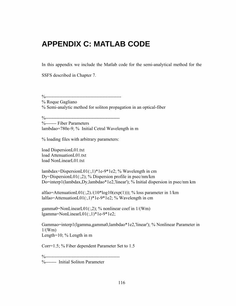
APPENDIX C: MATLAB CODE
In this appendix we include the Matlab code for the semi-analytical method for the
SSFS described in Chapter 7.
%------------------------------------------------- % Roque Gagliano % Semi-analytic method for soliton propagation in an optical-fiber %------------------------------------------------ %------- Fiber Parameters lambdao=780e-9; % Initial Cetral Wavelength in m % loading files with arbitrary parameters: load DispersionL01.txt load AttenuationL01.txt load NonLinearL01.txt lambdax=DispersionL01(:,1)*1e-9*1e2; % Wavelength in cm Dy=DispersionL01(:,2); % Dispersion profile in psec/nm/km Do=interp1(lambdax,Dy,lambdao*1e2,'linear'); % Initial dispersion in psec/nm km alfao=AttenuationL01(:,2)./(10*log10(exp(1))); % loss parameter in 1/km lalfao=AttenuationL01(:,1)*1e-9*1e2; % Wavelength in cm gamma0=NonLinearL01(:,2); % nonlinear coef in 1/(Wm) lgamma=NonLinearL01(:,1)*1e-9*1e2; Gammao=interp1(lgamma,gamma0,lambdao*1e2,'linear'); % Nonlinear Parameter in 1/(Wm) Length=10; % Length in m Corr=1.5; % Fiber dependent Parameter Set to 1.5 %------------------------------------------------ %------- Initial Soliton Parameter
116

c=3e8; % m/s To=[20:4:300]*1e-15 ; % Initial Soliton width (sec) vo=c/lambdao; % Initial Frequency (Hz) Po=(lambdao.^2).*(Do*1e-6)./(Gammao*2*pi*c*(To.^2)); %Initial Peak Power for Soliton %------------------------------------------------ Spams=1000; % Number of spans that the fiber is choped for j=1:length(To) % Initialization T(j,1)=To(j)*1e12; % To in psec l=Length/Spams*1e-3; % Spam Legnth in km lambda(j,1)=lambdao*1e2; % Units is cm v(j,1)=vo*1e-12; % Initial frequency in Thz D(j,1)=Do*1e2; % Initial dispersion in psec/cm2 P(j,1)=Po(j); for i=1:Spams, dv(j,i)=-((lambda(j,i).^2).*D(j,i)*133.58*Corr./(T(j,i).^4))*l; % Frequency Shift in THz v(j,i+1)=v(j,i)+dv(j,i); lambda(j,i+1)=(c./(v(j,i+1)*1e12))*1e2; % New lambda in cm D(j,i+1)=interp1(lambdax,Dy,lambda(j,i+1),'linear')*1e2; % Dispersion in psec/cm2 alfa(j,i+1)=interp1(lalfao,alfao,lambda(j,i+1),'linear'); % Attenuation in 1/km Gamma(j,i+1)=interp1(lgamma,gamma0,lambda(j,i+1),'linear'); T(j,i+1)=((lambda(j,i+1)^3).*D(j,i+1))./(Gamma(j,i+1)*2*pi.*c.*P(j,i).*exp(-alfa(j,i+1)*l).*lambda(j,i).*T(j,i))*1e12; % T in psec P(j,i+1)=(lambda(j,i+1)^2).*D(j,i+1)./(Gamma(j,i+1)*2*pi*c.*T(j,i+1)^2)*1e12; end end % Resuls display disp(T(:,1)) disp(P(:,1)) disp(T(:,Spams)*1e3) disp(P(:,Spams)) disp(-(v(:,Spams)-v(:,1))*1e3)
117

APPENDIX D: Submitted Publication
Some of the results of the work done for this Master Thesis were included in the
following article submitted for publication at OSA Optics Letters in April 2005.
Semi-analytical model of soliton self-frequency shift in an optical fiber
Roque Gagliano Molla, Student Member, IEEE and Rongqing Hui, Senior Member,
IEEE
Department of Electrical Engineering and Computer Science
The University of Kansas, Lawrence, KS 66045
Abstract:
A semi-analytical model is proposed to investigate the characteristics of soliton self-
frequency shift (SSFS) in optical fibers. SSFS in two different types of fibers were
evaluated and the results agree very well with those of numerical simulations. We
show that when the frequency shift is small enough, it is inversely proportional to the
fourth power of the initial soliton pulse width. However, with large frequency shift,
this fourth power rule needs to be modified.
Index Terms— Optical propagation in nonlinear media, optical soliton, Raman scattering.
118

I. Introduction
Soliton self frequency shift (SSFS) in optical fiber is due to the Stimulated Raman
Scattering (SRS). Once the pulse optical power level, the chromatic dispersion and
the fiber nonlinearity satisfy a well-known soliton condition, the Raman-shifted
optical pulses will be transformed into wavelength-shifted solitons and the amount of
SSFS can generally be adjusted by changing the power level of the optical pulses [1].
In recent years, new advances in high-power femtosecond fiber lasers and highly
nonlinear optical fibers have made SSFS more practical to obtain wavelength tunable
optical pulses. Because of its potential applications in optical communications and
biomedical imaging where wavelength tunability is desired, SSFS has been
investigated extensively. Experiments of SSFS in both 1550 – 2000nm and 780 –
1000nm wavelength regions have been reported [2, 3] and the results have been
analyzed both analytically and numerically.
The analytical formulation of Gordon [4] predicted that, the amount of SSFS ( )υ∆
is inversely proportional to the forth power of the FWHW optical pulse width ( )τ at
the fiber input, that is, . This result successfully explained the
experimental results reported in [1] where pulse width in the range of 420fs - 45ps
had been used. Although reference [4] provides a nice simple formula which predicts
the general behavior of SSFS, several effects were neglected such as fiber attenuation
and wavelength dependency of dispersion and nonlinearity. In fact, due to fiber
attenuation, the pulse peak power will be reduced and pulse width will be increased
while propagating along the fiber. As a result, the frequency shift tents to saturate as
demonstrated in [3]. In addition, as the central wavelength of an optical pulse shifts
while propagating along the fiber due to SSFS, its behavior will be determined by the
fiber parameters and the pulse energy at that specific wavelength. Because the amount
of SSFS is typically larger than 100nm, the wavelength dependent nature of
chromatic dispersion and nonlinearity may play important roles and they have to be
taken into account in theoretical calculations. On the other hand, numerical simulation
using split-step Fourier method has been proven to be effective and accurate to model
4, =∝∆ − xxτυ
119

the effect of SSFS. It has been used to predict the amount of wavelength shift versus
pulse optical power and pulse width. However, because femtosecond level pulse
widths are usually used, very wide bandwidth is required in the numerical simulation
and the process is generally very time-consuming. Another drawback of numerical
simulation is that it does not directly show the effects of various physical mechanisms
behind the results.
In this letter, we demonstrate a simple semi-analytic method to model SSFS in
optical fibers. By taking into account fiber attenuation and wavelength dependent
dispersion and nonlinearity, we show that the SSFS becomes less sensitive to the
input pulse width when this width is narrow enough and the fourth power rule
predicted in [4] may need to be modified for many practical applications. The results
of semi-analytic calculations are found to be in good agreement with numerical
simulations using split-step Fourier method. Our results also indicate that the fourth-
power rule predicted in [1] is accurate when the wavelength shift is small and the
fiber loss is negligible.
II. SEMI-ANALYTIC FORMULATION
Nonlinear optical pulse propagation in optical fibers can be modeled by an
extended nonlinear Schrödinger equation (NLS) in which the effect of Raman
scattering is included [5]:
( )
( ) ( ) ( ) ( ) ⎟⎟⎠
⎞⎜⎜⎝
⎛−⎟⎟
⎠
⎞⎜⎜⎝
⎛∂∂
+
=∂∂
−∂∂
+∂∂
++∂∂
∫∞+
∞−
'',',1
61
22
2
0
3
3
32
2
21
dtttzAtRtzAt
ii
tA
tAi
tAA
zA
ωωγ
βββωα
(1)
Where A(z, t) is the pulse envelope. The left-hand side represents the linear effects,
α is the fiber loss, β1 the group velocity, β2 and β3 the 1st order and the 2nd order
dispersions, respectively. The right-hand side represents the non-linear effects, where
γ is the nonlinear coefficient and R(t) is the response function that includes both the
electronic and the vibration (Raman) contribution [6,7]:
120

( ) ( ) ( ) ( )thftftR RRR +−= δ1 (2)
Where hR(t) is the Raman response function obtained from the Raman gain
spectrum of the fiber, fR represents the fractional contribution of the delayed Raman
response to nonlinear polarization.
When we neglect the fiber attenuation and consider that all fiber parameters are
independent of the wavelength, a closed-form analytical relationship between the
soliton central frequency shift and its initial pulse width can be found [4]:
( ) 4
20 /
oTD
KkmTHzz
λυ−=
∂∂
(3)
Where is the dispersion parameter in [ps/cm22 /2)( λβπλ cD −= 2], λ is the
wavelength in [cm] and T0 = τ /1.763 is the pulse width in [ps]. The proportionality
constant K is a fiber type- dependent parameter that is related to the value of the
Raman Gain. Although this analytical solution is simple, its derivation was based on a
single wavelength of the optical signal and therefore the wavelength dependency of
fiber parameters was not considered. Equation (3) is accurate when the amount of
pulse wavelength shift is small. In recently reported SSFS experiments, the pulse
wavelength shift can be as high as several hundred nanometers [3]. In this case, fixed-
wavelength approximation is no longer valid and eq.(3) needs to be modified.
Because different type of fibers may have very different wavelength dependency of
their key parameters, D(λ) and γ(λ) and α(λ), therefore, a closed-form analytical
solution may not be feasible. However, a semi-analytical formulation would be very
useful to significantly increase the speed of calculation compared to numerical
simulations, while maintaining excellent accuracy.
In order to obtain a semi-analytical solution, we truncate fiber into short sections,
within each section, a fixed signal wavelength can be assumed and fiber parameters at
this specific wavelength can be used. The optical frequency of a soliton passing
through a short fiber section from z to z + ∆z can be expressed as
( ) ( ) ( )( ) ( )( )
zzT
zzDKzzz
o
∆−=∆+ 4
2λλυυ (4)
121

Where )(zυ is the pulse optical frequency and T0(z) is the pulse width at the input.
D(λ(z)) is the fiber dispersion parameter at the wavelength λ(z). As SSFS is a non-
elastic effect, in addition to frequency shift, the peak power of the pulse also changes
after passing through the short section. This peak power change is caused by three
major effects, namely, fiber attenuation, pulse width change and energy loss of each
photon due to the red-shift of the wavelength. Therefore, the pulse peak power at the
output of the short fiber section is:
( ) ( ) ( )( )
( )( )zzT
zTz
zzezPzzP zzpp ∆+
∆+=∆+ ∆−
0
0))((
υυλα (5)
Where Pp(z) is the peak power at the input of the fiber section. Assuming a
fundamental soliton is maintained when pulses propagate along the fiber, the soliton
peak power is also related to its width by:
( ) ( )))(())((2
))((2
20 zz
zcDzTzPp λγλπυλ
= (6)
Combining equations (4 - 6), an expression of pulse width at z + ∆z can be obtained
as:
( ) ( )( )( )( ) ( ) ( ) ( ) ( )zTezPzzzc
zzDzzzzT zzzp 0
)(
3
0 2)(
∆∆+−∆+∆+∆+
=∆+ λαλλγπλλ
(7)
Where )(/)( zzczz ∆+=∆+ υλ is the wavelength of the pulse at the output of the
fiber section which can be obtained by equation (5); ))(( zzD ∆+λ , ))(( zz ∆+λγ and
))(( zz ∆+λα are the dispersion nonlinearity parameter and fiber attenuation,
respectively, evaluated at this new wavelength. With the parameters of a soliton pulse
know at the input, equations (5) and (7) can be used together to calculate the central
frequency and the pulse width of the wavelength shifted soliton at the output of a
short fiber section, these parameters can, in turn, be used as the input to the next fiber
section. SSFS characteristics of a long fiber can be obtained by dividing the fiber into
short sections and repeating this calculation section by section, along the fiber.
Because the transfer function of each fiber section described by equations (5) and (7)
122

is analytical, the calculation is straightforward and fast. In addition, since the
wavelength of the optical pulse at different fiber sections may be very different due to
SSFS, precise fiber parameters at each section can be used corresponds to the exact
signal wavelength at that section. This assures the accuracy of the calculation.
III. RESULTS AND DISCUSSION
In order to evaluate the accuracy of our semi-analytical model, the results were
compared with those of numerical simulations using VPI Transmission Marker [8]
where split-step Fourier method was used.
First we evaluated SSFS in a 100m polarization maintaining fiber (3M FS-PM-
7811) with wavelength dependent dispersion ( )75 1055.110877.11 −− ×−×+= λD in
[ps/nm2], where λ is in [cm], and wavelength-independent loss and
nonlinearity kmdB /6.2=α and ( )110044.0 −− ⋅= mWγ .The wavelength of the input
soliton pulse is set at 1550nm. Soliton frequency shift versus input optical pulse width
is shown in Fig.1, in which, results of semi-analytical calculation represented by
triangles agree well with those obtained by numerical simulations represented by
open circles. The vertical axis at the right indicates the exponent x. This parameter x
is equal to 4 when the pulse width is wide and the amount of frequency shift is small
as predicted by Gordon [4]. However, with pulse width narrower than 100fs, the
frequency shift becomes less sensitive to the pulse width and this slope can be
reduced significantly depending on fiber parameters. In this calculation, since the
fiber loss is only 0.26dB, for a 100m fiber-length, the impact in the results is
negligible. It needs to be mentioned that when the pulse width is narrower than 20fs,
the nonlinear Schrödinger equation (1) is no longer accurate because the narrowband
approximation fails [3] and that is beyond the scope of this work.
In order to show the effectiveness of this method, we also investigated SSFS in a
10m long photonic crystal fiber (PCF) with zero-dispersion wavelength at 710nm
[9,10]. The wavelength dependent fiber parameters are linearly interpolated from the
data listed in table 1. The wavelength of the input soliton pulses used in the
123

calculation is 780nm.
λ (nm) D (ps/nm/km) D slope (ps/nm2/km) γ (W-1 km-1) α (dB/km) 710 0 0.58 139 190
600 -142 1.70 171 210
800 68 0.59 122 170
1000 148 0.25 92 130
1550 185 -0.08 49 80
Table 1: Photonic Crystal Fiber NL-18-710 characteristics.
Fig. 2, shows the frequency shift versus soliton pulse width in the PCF calculated
by semi-analytical model (triangles) and numerical simulations (open cycles).
Because of the high loss in PCF, its impact cannot be neglected. To illustrate this
effect, soliton frequency shift calculated without fiber loss is also plotted in Fig.2
(squares) for comparison. Similar to what happened in the polarization maintaining
fiber, the exponent x is equal to 4 at relatively wide pulse width and is reduced
significantly when the pulse width is narrower than 100fs.
In all the cases, there is also agreement between the semi-analytical solution and
the numerical solution in both the output peak power and the output pulse width. The
output fundamental order of the soliton from the numerical solution was verified.
Fig.3 shows an example of the wavelength shift as a function of the fiber length for
different pulse widths calculated with semi-analytical model (continuous) and
numerical simulations. The results clearly show saturation in the frequency shift at
long fiber lengths as has been demonstrated experimentally [3]. The discrepancy
between semi-analytical model and numerical simulation when the pulse width is
narrower than 40fs is attributed to the effect of higher order dispersion, which is not
included in the semi-analytical model
IV. CONCLUSION
124

In this letter, we have introduced a semi-analytical method for the modeling of
SSFS in optical fibers. Calculation using this model is fast and is provides a better
understanding of the physical process involved. By comparing the calculated results
with numerical simulations in two different fiber types, the accuracy of semi-
analytical modeling is verified. When frequency shift is small enough, exponent x is
equal to 4, which agrees with previous works.
125

References
[1] F.M.Mitschke and L.F.Mollenauer, “Discovery of the soliton self-frequency shift”, Opt. Lett 11 (1986), 659-661.
[2] Norihiko Nishizawa, Youta Ito and Toshio Goto, “0.78-0.90-µm Wavelength-Tunable Femtosecond Soliton Pulse Generation Using Photonic Crystal Fiber”, Photonic Technology lett. 14 (2002) 986-988.
[3] Norihiko Nishizawa, Ryuji Okamura and Toshio Goto, “Analysis of Widely Wavelength Tunable Femtosecond Soliton Pulse Generation Using Optical Fibers” J. Appl. Phys. 38 (1999), 4768-4771.
[4] J.P. Gordon, “Theory of the soliton self-frequency shift”, Opt Lett. 11 (1986) 662-664.
[5] G. P. Agrawal, Nonlinear Fiber Optics, 3rd ed. New York: Academic, 2001.
[6] R.H. Stolen and W.J.Tomlinson, “Effect of the Raman part of the nonlinear refractive index on the propagation of ultrashort optical pulses infibers”, JOSA B 9 (1992), 565-573.
[7] R.H.Stolen, J.P.Gordon, W.J. Tomlinson and H.A. Haus, “Raman response function of silica-core fibers”, JOSA B 6 (1989) 1159-1166.
[8] VPI Photonics, VPI Transmission Maker, www.vpiphotonics.com.
[9] D.T. Reid, I.G. Cormack, W.J. Wadsworth,J.C. Knight and P.St.J. Russell, “Soliton Selft-frequency Shift Effect in Photonic Crystal Fibre”, CLEO 2002.
[10] M. Fuochi, F. Poli, S. Selleri, A. Cucinotta, and L, Vincetti, “Study of Raman amplification properties in triangular photonic crystal fibers”, J. Lightware Technol 21 (2003) 2247-2254.
126

Figure captions:
Fig. 1. Frequency shift versus pulse width for a 100m PMF in log scale. The straight
line represent the analytical result in [4], triangles the complete semi-analytical
solution and circles the numerical results. The figure also shows the difference
on the exponent x from the analytical value of 4
Fig. 2. Frequency shift and pulse width for a 10m PCF in log scale. The straight line
represent the analytical result in [4], squares the semi-analytical solution with no
losses, triangles the complete semi-analytical solution and circles the numerical
result. The figure also shows the difference on the exponent x from the
analytical value of 4.
Fig. 3. Wavelength shift and fiber length for a PCF for different soliton pulse widths.
Circles represent the numerical data.
127

Figure 1
1.5
2
2.5
3
3.5
4
4.5
1
6 10
dv (G
Hz)
20 40 60 80 100 15010
2
10 3
10 4
10 5
Pulse width (fsec)
x
128

Figure 2
20 40 60 80 Pulse Width (fsec)
100 15010
1
10 2
10 3
10 4
10 5
10 6
dvH
z)
(G
1.5
2
2.5
3
3.5
4
4.5
x
129

Figure 3
0 2 4 6 8 10780
785
790
795
800
805
810
815
Fiber Length (m)
Cen
ter W
avel
engt
h (n
m)
30 fsec40 fsec100fsec
Pulse Width
130
Related Documents