Nonlinear convection-dispersion models with a localized pollutant source, II - A class of inverse problems

ELSEVIER

Available online at www.sciencedirect.com MATHEMATICAL AND S¢,ENCE ~ ,D,n . -OT- COMPUTER

MODELLING Mathematical and Computer Modelling 42 (2005) 601-612

www.elsevier.com/locate/mcm

Nonl inear C o n v e c t i o n - D i s p e r s i o n M o d e l s wi th a Local ized Po l lu tant Source ,

I I - - A Class of Inverse P r o b l e m s

R. REVELLI AND L. RIDOLFI Department of Hydraulics

Politecnico di Torino, Torino, Italy <roberto. revell i><luca, ridolf i>©polit o. i~

(Received and accepted June 2004)

A b s t r a c t - - T h i s paper deals with the modelling and solution of a class of nonlinear inverse problems related to a transport diffusion model with a source term. Specifically, the first part of the paper deals with the description of the physical system and of the related mathematical problems. The second part deals with the development of the solution method which decomposes the space domain into a suitable set of subdomains. In each of them, the initial boundary value problem is direct and is solved by generalized collocation method. Combining the solutions in all domains gives the general solution to the inverse problem. Some simulations visualize the application of the method. @ 2005 Elsevier Ltd. All rights reserved.

Keywords--Nonl inear sciences, Transport processes, Diffusion, Direct, Inverse problems.

1. I N T R O D U C T I O N

This paper deals with the modelling and analysis of a class of inverse problems related to a

model, proposed in [1], describing nonlinear transport phenomena of chemicals in channels with

spatially variable properties with the addition of a nonlinear dispersion term and a localized

source. Referring to the contents of [1], which is going to be a constant reference to this present

paper, it is worth recalling that it deals with the above outlined modelling (with reference to the

classical literature [2-7]), and with the development of solution methods for direct problems.

Technically, the solution method is based on the the so-called generalized collocation method [8],

which is documented in various recent applications, e.g., [1,9,10]. In particular, the method

provides a useful discretization of continuous models and efficiently deals with nonlinearities

including the ones related to implicit boundary conditions. It diseretizes the original continuous

model (and problem) into a discrete (in space) model, with a finite number of degrees of freedom,

while the initial-boundary value problem is transformed into an initial-value problem for ordinary

differential equations. It is well understood that the method may provide an alternative to classical solution methods

for nonlinear equations for time evolution problems in one space dimension, while the initial-

boundary value problem is transformed into an initial-value problem for ordinary differential

Partially supported by Gruppo Nazionale Fisica Matematica of INDAM--Istituto Nazionale di Alta Matematica.

0895-7177/05/$ - see front matter @ 2005 Elsevier Ltd. All rights reserved. Typeset by .AA/~-~X doi:10, lO16/j.mcm.2004.06.023

602 R. REVELL[ AND L, RIDOLF[

equations. Then this system can be solved by standard methods for ordinary differential equations; see [11, Chapter II].

The analysis developed in [10] provides useful indications to deal with the estimate of the dis- tance between the true and the computational solution. Additional estimates can be obtained, as documented in [1], by comparison with analytic solutions. The method operates, as we shall see, efficiently even with stiff nonlinear problem. Nevertheless, it should be well understood that it is a technical alternative to classical solution methods for nonlinear partial differential equations, e.g., classical discretization schemes or Galerkin methods [12,13], which may be properly addressed to equations with source term [14]. The use of the software MATHEMATICA has shown to be able to deal efficiently with the solution of the initial-value problem for ordinary differential equations. Related programs can be recovered in [15].

This paper deals with the analysis of a class of inverse problems of interest for the applications. Specifically, we consider the case of models with localized source term such that both localization and time-evolution of the source are not known and have to be identified exploiting suitable measurements of the concentration of the chemical upstream and downstream from the source.

The contents are proposed through five sections, as follows.

• Section 1 deals with the above general introduction to the contents and to the aims of the paper.

• Section 2 deals with a concise summary of the class of transport and diffusion models in one space dimension with variable properties along the channel and nonlinear dispersion term. The model is the one proposed in [1], which, in particular, includes the presence of a distributed source term.

• Section 3 deals with the statement of the inverse problems which will be dealt with in this paper.

• Section 4 deals with the development of the mathematical method, based, as already mentioned, on the generalized collocation method [8]. This section refers to the classical literature on inverse problems for partial differential equations [1-18].

• Section 5 deals with some practical applications. • Section 6 indicates some research perspectives with special attention to the analysis of

relatively more sophisticated inverse problems.

2. M A T H E M A T I C A L P R O B L E M

The model considered in this paper was proposed in [1]. It describes the main transport processes that a chemical undergoes in a river according to

OC OT

[ 0c] _ o(v(()C)o( + K( ( )_5_( _ +

_ a c o 2 c + + cS(T)d(~ -- ~s), J

(2.1)

where ~ c [0, g] is the spatial coordinate, ~- E [0, T] is time, C E [0, Cmax] is the chemical concentration, and 5(.) is the Dirac delta function. In the above model, the advection, shear dispersion, nonlinear decay reaction, and a concentrated source term (located in ~s) in the case of a stream with spatially variable proprieties are retained. The functions are defined as h({) = ah(1 + ~/g) b'~ , v(~) = a,(1 + ~/g)bv, and K(~) = ag(1 + ~/g)bK. In the previous expressions, ah, bh, av, b~, ak, bk, A, m, and e are constants.

It is useful rewriting the differential equation (2.1) in a suitable dimensionless form such that all the independent and dependent variables are defined in the fundamental interval [0, 1]:

~- C = = = CM ( 2 . 2 )

Nonlinear Convection-Dispersion Models 603

where CM is the largest value of C, and where T is a critical t ime selected in order to yield lesser

or equal to one the coefficient of the term with higher (second) order space derivative. Technical

calculations yield Tak ~2

g2 = s - < l ~ T = e - - , (2.3) ak

where the choice of e is realized with the aim of keeping T consistent with time necessary to

observe the phenomena. The above change of variables leads to the following dimensionless equation:

Ou Ou c92u (~--'~- : [£1991(X) -- £2~2(X)] ~ + £3993(X)~X2 -- ]-t~t rn -- E4~4(2:)It n t- 7]S(t)t~(X -- 2:s) , (2.4)

where technical calculations yield

akbkT £1 -- ~2 ' ~1 -~" (1 -I- X) bk-1, (2.5a)

avT e 2 = e ' P 2 = ( I + x ) b', (2.5b)

akr ~1 = (1 + z) (2.5c) E3 -- g2 bk'

%bvT e4 - ~ - e2bv, ~4 = (1 + x) by-l, (2.5d)

and

(2.5e) # = A C ~ - I T , ~ - - C M .

The source term s(t) is concentrated at the position x = x~, with 0 < x~ < 1. Let us indicate with u(t ,x = 0) = c~(t) and u(t ,x = 1) = ~(t) the Dirichlet-type boundary conditions and with u(t = 0, x) = 7(x) the initial condition. Moreover, in the inverse problems, a measure of

concentration u.(t) = u(t ,x,) (or u*(t) = u(t,x*)) is known, with 0 < x . < x~ (x~ < x* < 1).

3. S T A T E M E N T OF I N V E R S E P R O B L E M

In the present paper, we propose a solution technique for the following three problems.

PROBLEM 1. Compute u(t, x) with given c~(t),/3(t), and s(t).

PROBLEM 2. Compute s(t) and u(t, x) with given a(t) , ~(t), u.(t) (or u*(t)).

PROBLEM 3. Compute ~(t) and u(t,x) with given c~(t), s(t), and u*(t).

Problem 1 is a direct problem that we consider for two reasons: to test the technique of domain decomposition (used in the inverse problems) for a model like (2.4) and to provide the

numerical input for the other two problems. Problems 2 and 3 are inverse problems; the first one is the most interesting problem from a physical point of view and it has the aim of finding the unknown temporal evolution of the source being known its spatial position, the concentration in a downstream (or upstream) point, and the boundary conditions. Differently, Problem 3 deals

with the research of the downstream boundary condition given the source term. In order to solve the previous three problems, a domain decomposition is adopted, that is, the

domain D = [0, 1] of the space variable is decomposed in subdomains as follows:

D --- [0, 1] = D1 u D2 U D3. - - , (3.1)

where the definition of the subdomains depends on the specific problem considered. The variable u

in the r th subdomain, Dr, is identified by the apex, i.e., u (r), and in each subdomain a suitable collocation I (~),

i = 1 , . . . , n ~ : I (r) x r ) , . . . ,~ , i , . . . , x ,

604 R. REVELLI AND L. RIDOLFI

is defined. On this basis, the two following numericM schemes will be used in the following section for the solution of the problems.

SCHEME 1. DIRICHLET PROBLEM. Two-points Dirichlet problem with collocation in space and integration in time.

The variable u(t, x) is interpolated and approximated in the corresponding collocation by

~(t, ~) ~ ~ ( t , z) = ~ L~(z>~(t), (a.2) i=1

where ~(t) = ~(z~, t) and L~(~) ~re generic fundamental (spatial) interpotants. SCHEME 2. INITIAL VALUE PROBLEM. Initial value problem with collocation in time and integration in space.

The variable u(t, x) is interpolated and approximated in the corresponding collocation by

~(t, ~) ~ ~ ( t , ~) = ~ &(t)~(~), (a.a) i=1

where ui(x) = u(x , ti) and Si(t) are generic fundamental (temporal) interpolants.

4. M A T H E M A T I C A L M E T H O D

The solution of Problem 1 goes through the following steps.

STEP 1 .1 . W e u s e the domain decomposition

D = [0, 11 = 191 U D2 = [0, xs] U [ms, 1], (4.1)

with Chebyschef-type collocations, namely,

i = 1 , . . . , r t I : ----" - ~ - " " " ~ i , . . . , X ~ X s ,

xo 1)! 1 + cos 2 [ nl

(4.2a)

for the D1 and

i = 1 , . . . , n2 : (2) x 2 ) - = x s , . . . , ~ c i , " ' , n2 '

-_ (I [~(i-i)] (4.2b)

for the D2. Scheme 1 is used for both D1 and D2, and the dependent variable u (~) = u(~)(t, x) is interpo-

lated and approximated by means of the values ul ") (t) -- u (~) (t, xl r)) using Lagrange polynomials as follows:

n,r

u(~) (t, x) ~ ~(~)"~ (t, ~) = ~ L~ ~) (:~)~)(~), (4.3) j = l

where r = 1,2, ulr)(t) = u(r)(t, xlr)), and

L~f )(x) - i=l,i#j

j = l

(4.4)


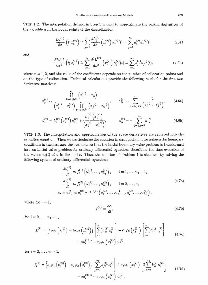
STEP 1.2. The interpolation defined in Step I is used to approximate the partial derivatives of the variable u in the nodal points of the discretization

Ou(~) ~,~ (~) ~,~ ( o~ t;x~ ~ )_2 ~ :~ C)(t) =2_,%~ (~)~j (~)(t) j = l j = l

(4.5~)

and

02~t(v) ( ) d Lj r)(t) ~"~i(v) (r) i.\ = 2_.., oj~ u j t~) , (4.5b)

d x 2 j = l j = l

where r = 1, 2, and the value of the coefficients depends on the number of collocation points and on the type of collocation. Technical calculations provide the following result for the first two derivative matrices:

a(r) = p = l , p • i , _(r) 1 , (4.6a)

p=l,pT~j

aji • uji + (xj~.)_xl,.)) b~ =-j=l,y#iE (4.6b)

S T E P 1.3. The interpolation and approximation of the space derivatives are replaced into the evolution equation. Then we particularize the equation in each node and we enforce the boundary conditions in the first and the last node so that the initial-boundary value problem is transformed into an initial value problem for ordinary differential equations describing the time-evolution of the values u i ( t ) of u in the nodes. Thus, the solution of Problem 1 is obtained by solving the following system of ordinary differential equations:

du~l) - f }L) (u~ ' ) .. u(1)) i=I , . ,n,- l , dt " ' ' ""

d t "" ' ' "

, . . . ~Unl_l~U 2 ~ . . .~

(4.7a)

where for i = 1,

for i = 2 , . . . , n l - 1,

f ~ l ) d a d t '

(4.7b)

[~-~ (1)(i)I ['~'~.(i) (1)l f}l) _ [~I~1 (X~ I)) --~2~fl2 (XlI))] l~__~aji uj I +E3~fla (X~ I)) [j~_lOJi uj J L j=~ J (4.7c)

for i ---- 2 , . . . , n 2 - - 1,

Oji ~tj (4.7d)


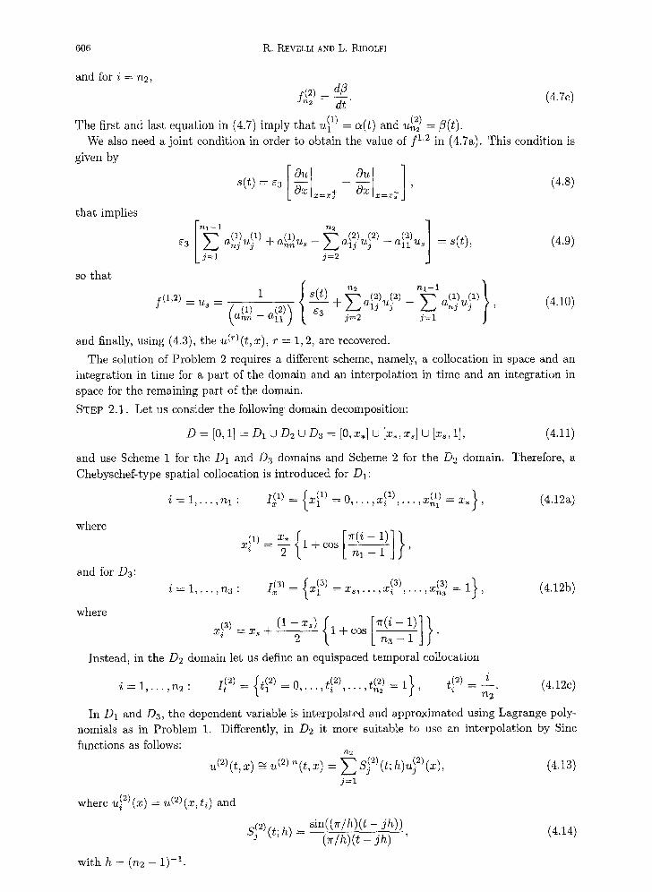
and for i : n2, f,(2) d~ = ( 4 . 7 e )

The first and last equation in (4.7) imply that u~ z) c~(t) and ~ (2) = = 9 ( t ) .

We also need a joint condition in order to obtain the value of fL2 in (4.7a). This condition is given by

[ Ou =x+ Ou ] (4.8) s(t)=~3 ~ O~=~: '

that implies

so that

(1) ( 1 ) . ~ a ( 1 ) u ~ (2) ( 2 ) _ a ( 2 ) u ~3 anj ~Zj nn s -- L~ alj ~J 11 s

L j=l j=2 = s(t), (4.9)

n l _ 1 } 1 s(t) + ~ (2)(2) (~) (1)

-- - - - ~ alj Uj -- E anj Uj , f(1,2) = Us [aO) ,~(2)'~ ¢3 (4.10) i x a n '~11 ) j=2 j = l

and finally, using (4.3), the u(~)(t, x), r = 1, 2, are recovered.

The solution of Problem 2 requires a different scheme, namely, a collocation in space and an integration in time for a part of the domain and an interpolation in time and an integration in space for the remaining part of the domain.

STEP 2.1. Let us consider the following domain decomposition:

D = [0, 1] = D, U D2 U Da = [0, x,] U [x., x~] U [Xs, 1], (4.11)

and use Scheme 1 for the D1 and Da domains and Scheme 2 for the D2 domain. Therefore, a Chebyschef-type spatial collocation is introduced for DI:

i : 1 , . . . , n 1 : /-(1) : {X[ 1) :0 , . . . ,x i - (1) , . . . ,x (1) : X , } , (4.12@

where

and for D3:

:-y 1+eost j '

. ={ [ -x (3) x(3)=1} i : 1, . . , n3 : I (3) x 3) : ms,.. , i , • - •, na , (4.12b)

where x} 3 ) = x s + ( 1 - x j 1 + c o s - -

2 / na 1

Instead, in the D2 domain let us define an equispaced temporal collocation

i=1, Ip {¢)=0, ,¢) I412o) . . . ~ ~ . . . , . . . ~ n 2 , - - n2

In D1 and D3, the dependent variable is interpolated and approximated using Lagrange polynomials as in Problem 1. Differently, in D2 it more suitable to use an interpolation by Sinc

functions as follows: n2 = Sj (t;h)u~2)(x), (4.13)

j = l

where ~ (2) ~i (x) = u (2)(x, ti) and

S} 2) (t; h) = sin((fr/h)(t - jh)) (4.14) (;r/h)(t - jh) '

with h = (n2 - 1) -1.


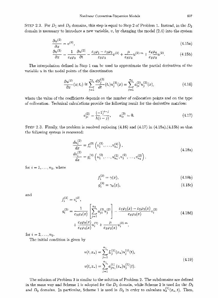
STEP 2.2. For D1 and D3 domains, this step is equal to Step 2 of Problem 1. Instead, in the D2 domain is necessary to introduce a new variable, v, by changing the model (2.4) into the system

0u (2) - v (2), (4.15a)

0x

Ov (2) _ 1 Ou (2) ~1~1 -E2~2v(2) + # u(2),~ + s4~4u(2). (4.15b) 0X K3(~P 3 0 t E3~ 3 E3~O 3 E3~ 3

The interpolation defined in Step 1 can be used to approximate the partial derivatives of the variable u in the nodal points of the discretization

~2 dS! 2) n2 Ou(2)(x;t~)Ox ~- Y~"L~t (t~)u~2)(x) = ~ ai,(2) Uy(2)" "(x), (4.16)

j = l j = l

where the value of the coefficients depends on the number of collocation points and on the type of collocation. Technical calculations provide the following result for the derivative matrices:

a~2) - ( - 1 ) i - / _(2) = 0 . (4 .17)

STEP 2.3. Finally, the problem is resolved replacing (4.16) and (4.17) in (4.15a),(4.15b) so that the following system is recovered:

du~ 2) = f~2)(V~), V(2)

dx " " ' ~ / '

dx - Yi . . , n2 , ~l , ' ' ' , n: ] ~

(4.1Sa)

for i = 1 , . . . , n2~ where

f } :) = (4.18b)

(4.18c)

and f(2) = v}2)

I

A . (2) + + 3w(x) '

for i = 2 , . . . , n 2 .

The initial condition is given by

(4.18d)

nl = nj (x , )u j (t),

j = l nl

V(t ,X.) ~-~ E -(1)(tin I ( x . ) ~ l ) ( t ) .

j = l

(4.19)

The solution of Problem 3 is similar to the solution of Problem 2. The subdomains are defined in the same way and Scheme 1 is adopted for the D1 domain, while Scheme 2 is used for the D2 and Da domains. In particular, Scheme 1 is used in D1 in order to calculate u(1)(x, , t ) . Then,


Scheme 2 in D2 allows us to obtain us, u(~2)(xs, t), and, by means of the joint condition (3.10),

u(3)(xs, t). Finally, by applying Scheme 2 in the D3 domain, the boundary condition ~(t) is recovered.

REMARK 1. The solution methods proposed for the inverse Problems 2 and 3 can be easily applied also when the measure, u*(t), is localized downstream from the source, that is, x* > x~. In this case, it is sufficient to define the following domain decomposition:

D = [0, 1] = D1 U D2 U D3 = [0, xs] U [xs, x*] U [x*, 1], (4.20)

and to apply the same steps proposed for the Problem 2 or 3, respectively.

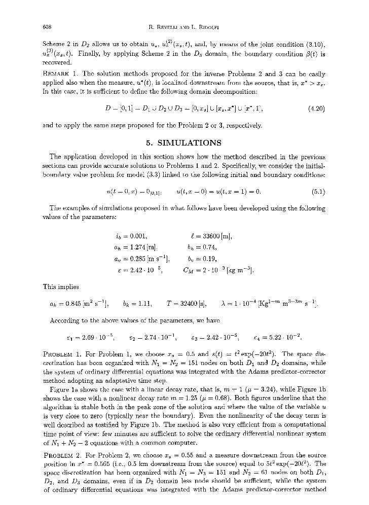
5. S I M U L A T I O N S

The application developed in this section shows how the method described in the previous sections can provide accurate solutions to Problems 1 and 2. Specifically, we consider the initial- boundary value problem for model (3.3) linked to the following initial and boundary conditions:

= 0 , x ) = %,1] , (5 .1 )

The examples of simulations proposed in what follows have been developed using the following values of the parameters:

ib = 0.001,

ah = 1.274 [m],

a~ = 0.285 [m s-l] ,

s = 2.42- 10 -5,

= 33600 [m],

bh = 0.74,

b~ = 0.19,

CM = 2 .1 0 -3 [kg m-3].

This implies

ak = 0.845 [m 2 s- l] , bk = 1.11, T = 32400 [s], A = 1 .1 0 -4 [Kg 1 -~ m 3-a'~ s-l] .

According to the above values of the parameters, we have

£1 = 2.69.10 -5, ~2 = 2.74.10 -1, £3 = 2.42.10 -5, ~4 ---- 5 .22.10 -2.

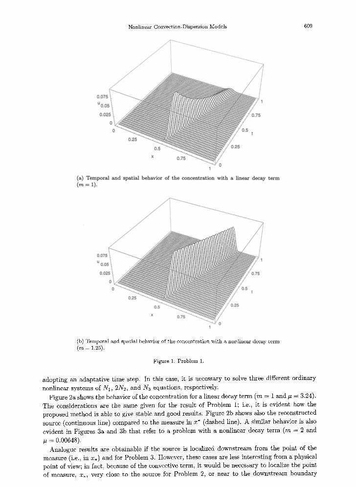
PROBLEM 1. For Problem 1, we choose xs = 0.5 and s(t) = t 2 exp(-20t2) . The space discretization has been organized with N1 = N2 = 151 nodes on both D1 and D~ domains, while the system of ordinary differential equations was integrated with the Adams predictor-corrector method adopting an adaptative time step.

Figure l a shows the case with a linear decay rate, that is, rn = 1 (# = 3.24), while Figure lb shows the case with a nonlinear decay rate m = 1.25 (~ = 0.68). Both figures underline that the algorithm is stable both in the peak zone of the solution and where the value of the variable u is very close to zero (typically near the boundary). Even the nonlinearity of the decay term is well described as testified by Figure lb. The method is also very efficient from a computational

time point of view: few minutes are sufficient to solve the ordinary differential nonlinear system

of N1 + N2 - 2 equations with a common computer.

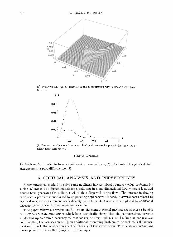
PROBLEM 2. For Problem 2, we choose xs = 0.55 and a measure downstream from the source position in x* = 0.565 (i.e., 0.5 km downstream from the source) equal to 5t 2 exp(-20t2) . The space discretization has been organized with N1 = N3 = 151 and Na = 61 nodes on both D1, D2, and D3 domains, even if in D2 domain less node should be sufficient, while the system of ordinary differential equations was integrated with the Adams predictor-corrector method


0.075

u 0.05

0.02!

1

(a) Temporal and spatial behavior of the concentration with a linear decay term ( .~ = 1).

l

0.075

U 0.05

0.02~

1

(b) Temporal and spatial behavior of the concentration with a nonlinear decay term (m = 1.25).

Figure 1. Problem 1.

adopting an adaptative time step. In this case, it is necessary to solve three different ordinary

nonlinear systems of N1, 2N2, and Ns equations, respectively.

Figure 2a shows the behavior of the concentration for a linear decay term (m --- 1 and # = 3.24). The considerations are the same given for the result of Problem 1; i.e., it is evident how the proposed method is able to give stable and good results. Figure 2b shows also the reconstructed

source (continuous line) compared to the measure in x* (dashed line). A similar behavior is also

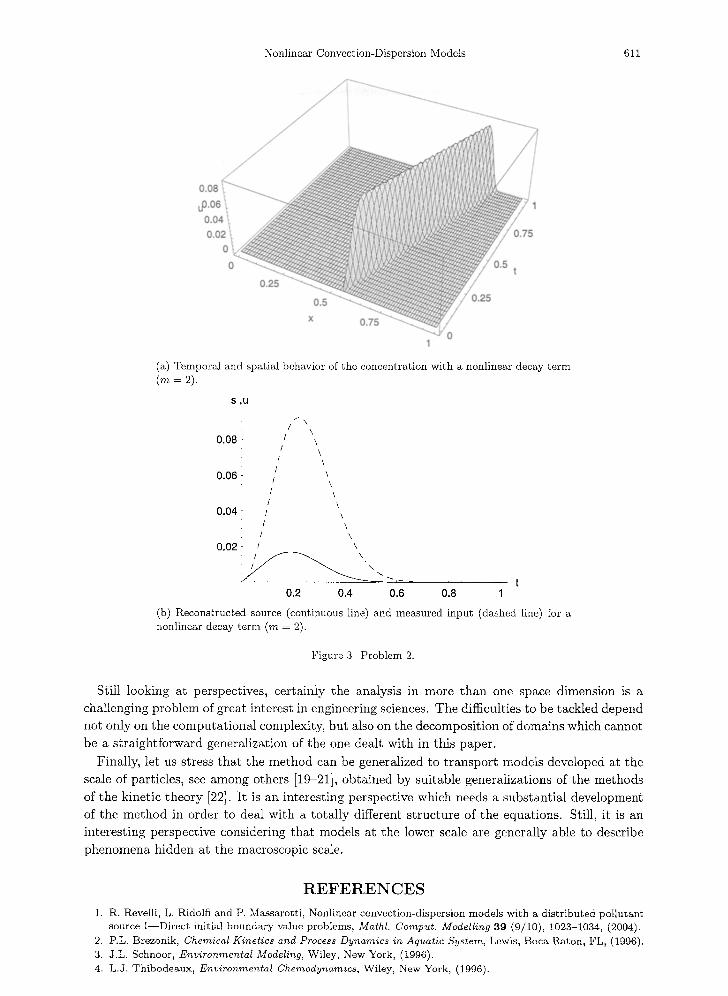
evident in Figures 3a and 3b that refer to a problem with a nonlinear decay term (m = 2 and

p = 0.00648). Analogue results are obtainable if the source is localized downstream from the point of the

measure (i.e., in x , ) and for Problem 3. However, these cases are less interesting from a physical point of view; in fact, because of the convective term, it would be necessary to localize the point of measure, x . , very close to the source for Problem 2, or near to the downstream boundary


0.1

0.075 U

0.0~

0.02.

(a) Temporal and spatial behavior of the concentration with a linear decay term (m ---- 1).

S , U

f \ , / i / \

0 .08 r \ / \

0 .06 I \ ! \

! \ 0 .04 1 / \

F f \

I ! \ , . 0.2 0 .4 0 ,6 0 .8 1

(b) Reconstructed source (continuous line) and measured input (dashed line) for a linear decay term (rn = 1).

Figure 2. Problem 2.

for Problem 3, in order to have a significant concentration u. (t) (obviously, this physical limit

disappears in a pure diffusive model).

6. CRITICAL ANALYSIS A N D P E R S P E C T I V E S

A computat ional method to solve some nonlinear inverse init ial-boundary value problems for a class of t ranspor t diffusion models for a pollutant in a one-dimensional flow, where a localized

source te rm generates the pollutant which then dispersed in the flow. The interest in dealing with such a problem is motivated by engineering applications. Indeed, in several eases related to applications, the measurement is not directly possible, while it needs to be replaced by additional

measurements related to the dependent variable.

This paper follows a previous one [1], where the computat ional method has shown to be able to provide accurate simulations which have technically shown that the computat ional error is controlled up to desired accuracy at least for engineering applications. Looking at perspectives and recalling the last section of [1], an additional interesting problem to be tackled is the identi- fication of both the localization and the intensity of the source term. This needs a nonstandard development of the method proposed in this paper.


0.08 uO.06 O.Oz 0.0

(a) Temporal and spatial behavior of the concentration with a nonlinear decay term (m = 2).

0.08

0.06

0.04

0.02

S ,U

f \ /

\ /

\ !

\ / \

/ \ t \

/ \ I \

/ \ / \

/ \

/ k

~ - - t 0.2 0.4 0.6 0.8 1

(b) Reconstructed source (continuous line) and measured input (dashed line) for a nonlinear decay term (m = 2).

Figure 3, Problem 2.

Still looking at perspectives, certainly the analysis in more than one space dimension is a

challenging problem of great interest in engineering sciences. The difficulties to be tackled depend

not only on the computa t iona l complexity, bu t also on the decomposi t ion of domains which cannot

be a s t ra ight forward generalization of the one dealt with in this paper.

Finally, let us stress t ha t the me thod can be generalized to t r anspor t models developed at the

scale of particles, see among others [19-21], obta ined by suitable generalizations of the methods

of the kinetic theory [22]. I t is an interesting perspective which needs a substant ia l development

of the me thod in order to deal with a to ta l ly different s t ruc ture of the equations. Still, it is an

interesting perspective considering tha t models at the lower scale are generally able to describe

phenomena hidden at the macroscopic scale.

R E F E R E N C E S

1. R. Revelli, L. Ridolfi and P. Massarotti, Nonlinear convection-dispersion models with a distributed pollutant source I--Direct initial boundary value problems, MathL Comput. Modelling 39 (9/10), 1023-1034, (2004).

2. P.L. Brezonik, Chemical Kinetics and Process Dynamics in Aquatic System, Lewis, Boca Raton, FL, (1996). 3. J.L. Schnoor, Environmental Modeling, Wiley, New York, (1996). 4. L.J. Thibodeaux, Environmental Chemodynamics, Wiley, New York, (1996).


5. R.P. Schwarzenbach, P.M. Gschwend and D.M. Imboden, Environmental Organic Chemistry, Wiley, New York, (1998).

6. K.R. Rajagopal and L. Tao, Mechanics of Mixtures, World Sci., Singapore, (1995). 7. A. Maraseo and A. Romano, Balance laws in charged continuous systems with an interface, Math. Mod.

Meth. Appl. Sci. 12, 903-920, (2002). 8. N. Bellomo, Nonlinear models and problems in applied sciences: From differential quadrature to generalized

collocation methods, Mathl. Comput. Modelling 26 (4), 13-34, (1997). 9. L. Ridolfi and R. Revelli, Sinc collocation-interpolation method for the simulation of nonlinear waves, Com-

puters Math. Applic. 46 (8/9), 1443-1453, (2003). 10. N. Bellomo, E. De Angelis, L. Graziano and A. Romano, Solution of nonlinear problems in applied sciences by

generalized collocation methods and Mathematica, Computers Math. Applic. 41 (10/11), 1343-1363, (2001). 11. N. Bellomo and L. Preziosi, Modelling Mathematical Methods and Scientific Computation, CRC Press, Boca

Raton, FL, (1995). 12. B. Di Martino, F. Flori, C. Giacomoni and P. Orenga, Mathematical and numerical analysis of a tsunami

problem, Math. Mod. Meth. Appl. Sci. 13, 1489-1514, (2003). 13. J. Valenciano and M.A.J. Chaplain, Computing highly accurate solutions of a tumor angiogenesis model,

Math. Mod. Meth. Appl. Sci. 13, 747-769, (2003). 14. E. Lorin and V. Seignole, Convection systems with stiff source term, Math. Mod. Meth. Appl. Sci. 13,

971-1019, (2003). 15. N. Bellomo, L. Preziosi and A. Romano, Mechanics and Dynamic Systems with Mathematica, Birkhguser,

Boston, MA, (2000). 16. J. Back, B. Blackwell and C. St. Clair~ Inverse Heat Conductions, Wiley, London, (1985). 17. M.M. Lavrent'ev, K.C. Reznitskaya and V.G. Yakhno, One-Dimensional Inverse Problems of Mathematical

Physics, American Mathematical Society Translations, Volume 130, Providence, RI, (1985). 18. D. Colton, R. Ewing and W. Rundell, Inverse Problems in Partial Differential Equations, SIAM, Philadel-

phia, PA, (1995). 19. C. Croizet and R. Catignol, Boltzmann-like modelling of a suspension, Math. Mod. Meth. Appl. Sci. 12,

943-964, (2002). 20. A. Bellouquid, A diffusive limit for nonlinear discrete velocity model, Math. Mod. Meth. Appl. Sci. 13, 35-58,

(2002). 21. M. Mokhtar-Kharroubi, Homogenization of boundary value problems and spectral problems for neutron

transport in local periodic media, Math. Mod. Meth. Appl. Sei. 14, 47-79, (2004). 22. L. Arlotti, N. Bellomo and E. De Angelis, Generalized kinetic (Boltzmann) models: Mathematical structures

and applications, Math. Mod. Meth. Appl. Sci. 12, 567-591, (2002).

Nonlinear convection-dispersion models with a localized pollutant source, II - A class of inverse problems

Documents