Nonlinear Control of Variable Speed Wind Turbines with Swithcing Across Operating Regimes

Nonlinear Control of Variable Speed Wind Turbines

With Switching Across Operating Regimes

Tuhin Das∗

Mech. Matls. & Aero. Engg. Dept.

University of Central Florida

Orlando, FL 32816

Email: [email protected]

Greg Semrau

Southwest Wind Power

1801 W Rt 66

Flagstaff AZ 86001

Sigitas Rimkus

Mech. Matls. & Aero. Engg. Dept.

University of Central Florida

Orlando, FL 32816

Abstract

One of the key control problems associated with variable speed wind turbines is

maximization of energy extraction when operating below the rated wind speed and

power regulation when operating above the rated wind speed. In this paper, we ap-

proach these problems from a nonlinear systems perspective. For below rated wind

speeds we adopt existing work appearing in the literature and provide further insight

into the characteristics of the resulting equilibrium points. For above rated wind speeds,

we propose a nonlinear controller and analyze the stability property of the resulting

∗Address all correspondence to this author.

1

equilibria. We propose a method for switching between the two regimes that ensures

continuity of control input at the transition point. We perform an analytical study of

the stability of the equilibria of the closed loop system under switching control. The

control laws are verified using a wind turbine model with two different wind speed

profiles.

1 Introduction

With the growing energy demand and need to decrease greenhouse gas emissions, renewable

energy systems are poised to become a large part of energy generation. One of the most

popular renewable energy systems over the past decade has been the wind turbine. Tech-

nological advances in modeling, prediction, sensing and control combined with the current

shift towards decentralized power have prompted development of wind energy systems. Al-

though initial expenditures could be an issue, the overall costs of installing and running wind

turbines are rapidly reducing with technological advances [4]. There are two different main

types of wind turbines, horizontal axis and vertical axis wind turbines [4, 9]. The focus of

this work in on horizontal axis wind turbines (HAWTs). There are two primary classifica-

tions of HAWTs, fixed speed and variable speed. The fixed speed system is easy to build and

operate but variable speed system provides greater energy extraction, up to a 20% increase

over fixed speed [4]. However, recent advances in fixed speed wind turbines augmented with

a variable ratio gearbox promises greater energy extraction [7]. The variable speed system

on the other hand requires more sophisticated controllers, which is an area of active research

[1].

From a systems perspective, energy is injected into the turbine through the torque gener-

ated at the turbine rotor due to wind velocity. Energy is extracted by drawing current from

the generator, which effectively provides a braking torque. In addition, the amount of wind

energy extracted can be modulated by varying the pitch angles of the rotor blades. The

generator torque (or current draw) and the blade pitch angle can be considered as control

2

inputs. A variable speed wind turbine operates differently in different operating regimes,

as shown in Fig.3, see [14, 11]. These operating regimes are explained in detail in the sec-

tion titled Operating Regimes. The main regimes of operation are, below rated wind speed

(regime 2, Fig.3) and above rated wind speed (regime 3, Fig.3). A significant amount of

work has been reported in the literature for regime 2 operation where maximization of the

extracted power is the main objective [3, 11, 5, 8, 10]. Typical control designs maintain the

wind turbine at a specific optimal operating point. In scenarios where this operating point

may not be exactly known or could change with time, it is adaptively identified using an

augmented parameter estimation algorithm.

Control designs proposed for regime 3 operations are relatively fewer in the literature.

In [2], the authors propose a cascaded generator torque controller. In both [1] and [17], the

authors propose multi-variable control in regime 3, employing both blade pitch and generator

torque as control inputs. Here the objective is to maintain relatively uniform generator torque

and thereby maintain uniform rotor speeds while achieving power regulation. As control

algorithms for the two regimes are considerably different, switching between controllers must

be handled carefully. There is very limited amount of work in the literature that addresses

the switching aspect. In [17], the authors propose a transition method that interpolates

between their regime 2 and 3 generator control torques, based on the current rotor speed.

In this paper, we address the control of a variable speed wind turbine from a nonlinear

systems perspective. For regime 2 operation, we do not attempt to develop a new control

algorithm. However, with the controller of [11] as a baseline algorithm, we provide further

insight into the characteristics of the equilibrium points and obtain a limiting operating

point. For regime 3 operation, we propose a simple nonlinear control and investigate the

stability of the equilibrium. As in regime 2, the proposed regime 3 controller also results in

two equilibrium points, of which one is stable and the other is unstable. We further determine

the region of attraction of the stable equilibrium points in each regime. We next propose

a method for switching between controllers based on rotor speed that ensures continuity of

3

rotor speed at the transition point. We analyze the implication of switching on the stability

of the closed loop system under the switching control. The paper is organized as follows.

First the system model is described. This is followed by a discussion on control development

where we first discuss the operating regimes and then present the control algorithms for

regimes 2 and 3. Switching between regimes is discussed next. Subsequently, an analysis

of the stability of the resulting equilibria under switching control is presented. Simulation

results are provided next and finally concluding remarks are presented.

2 System Model

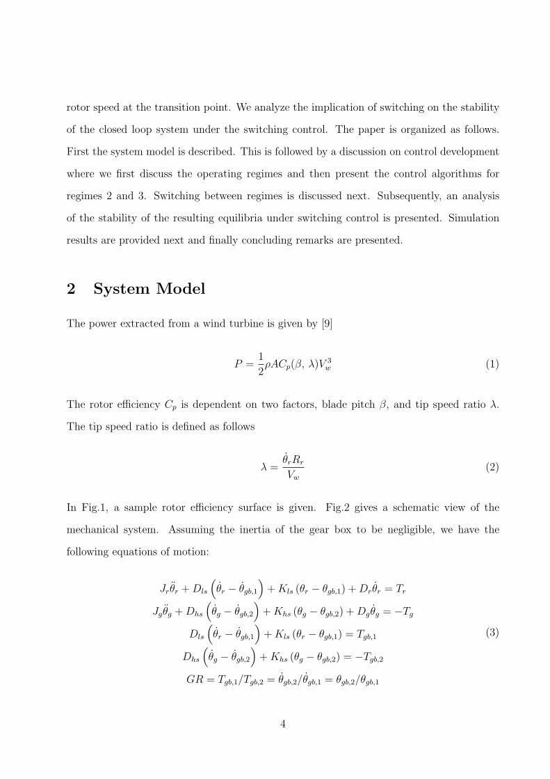
The power extracted from a wind turbine is given by [9]

P =1

2ρACp(β, λ)V

3w (1)

The rotor efficiency Cp is dependent on two factors, blade pitch β, and tip speed ratio λ.

The tip speed ratio is defined as follows

λ =θ̇rRr

Vw

(2)

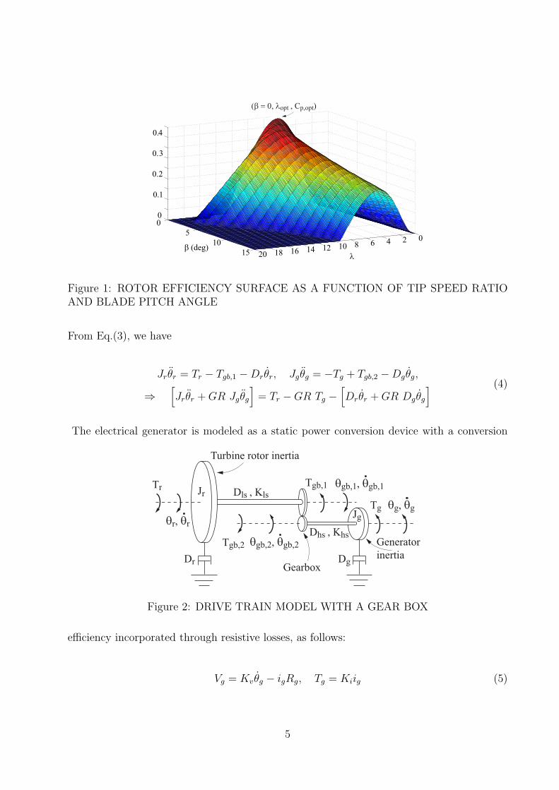
In Fig.1, a sample rotor efficiency surface is given. Fig.2 gives a schematic view of the

mechanical system. Assuming the inertia of the gear box to be negligible, we have the

following equations of motion:

Jrθ̈r +Dls

(θ̇r − θ̇gb,1

)+Kls (θr − θgb,1) +Drθ̇r = Tr

Jgθ̈g +Dhs

(θ̇g − θ̇gb,2

)+Khs (θg − θgb,2) +Dgθ̇g = −Tg

Dls

(θ̇r − θ̇gb,1

)+Kls (θr − θgb,1) = Tgb,1

Dhs

(θ̇g − θ̇gb,2

)+Khs (θg − θgb,2) = −Tgb,2

GR = Tgb,1/Tgb,2 = θ̇gb,2/θ̇gb,1 = θgb,2/θgb,1

(3)

4

02468101214161820

0

5

10

15

0

0.1

0.2

0.3

0.4

λβ (deg)

(β = 0, λopt , Cp,opt)

Figure 1: ROTOR EFFICIENCY SURFACE AS A FUNCTION OF TIP SPEED RATIOAND BLADE PITCH ANGLE

From Eq.(3), we have

Jrθ̈r = Tr − Tgb,1 −Drθ̇r, Jgθ̈g = −Tg + Tgb,2 −Dgθ̇g,

⇒[Jrθ̈r +GR Jgθ̈g

]= Tr −GR Tg −

[Drθ̇r +GR Dgθ̇g

] (4)

The electrical generator is modeled as a static power conversion device with a conversion

Tr

θr, θr

Dls , Kls

Tgb,1 θgb,1, θgb,1

Dhs , KhsTgb,2 θgb,2, θgb,2

Tg θg, θg

Dr Dg

Jr

Jg

Turbine rotor inertia

Generator

inertiaGearbox

Figure 2: DRIVE TRAIN MODEL WITH A GEAR BOX

efficiency incorporated through resistive losses, as follows:

Vg = Kvθ̇g − igRg, Tg = Kiig (5)

5

where Vg is the generator voltage, Kv is the generator emf constant, ig is the generator

current, Rg is the generator internal resistance, and Ki is the generator torque constant.

3 Control Development

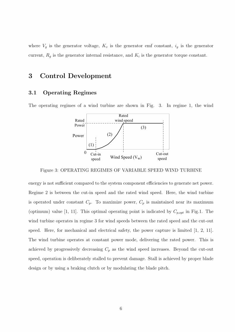
3.1 Operating Regimes

The operating regimes of a wind turbine are shown in Fig. 3. In regime 1, the wind

0Wind Speed (Vw)

Power

Rated

Power

Rated

wind speed

Cut-in

speed

Cut-out

speed

(1)

(2)

(3)

Figure 3: OPERATING REGIMES OF VARIABLE SPEED WIND TURBINE

energy is not sufficient compared to the system component efficiencies to generate net power.

Regime 2 is between the cut-in speed and the rated wind speed. Here, the wind turbine

is operated under constant Cp. To maximize power, Cp is maintained near its maximum

(optimum) value [1, 11]. This optimal operating point is indicated by Cp,opt in Fig.1. The

wind turbine operates in regime 3 for wind speeds between the rated speed and the cut-out

speed. Here, for mechanical and electrical safety, the power capture is limited [1, 2, 11].

The wind turbine operates at constant power mode, delivering the rated power. This is

achieved by progressively decreasing Cp as the wind speed increases. Beyond the cut-out

speed, operation is deliberately stalled to prevent damage. Stall is achieved by proper blade

design or by using a braking clutch or by modulating the blade pitch.

6

3.2 Below Rated Wind Speed - Regime 2

As discussed in the Introduction, control design for regime 2 is thoroughly addressed in the

literature. We do not attempt to develop a new control design for this regime. Rather, we

focus on the stability analysis of the closed loop system. First, a commonly used simplified

form of Eq.(4) is obtained by neglecting the compliance between θr and θg, which implies

from Eq.(3) and from Fig.2,

θ̇g = θ̇gb,2 = GR θ̇gb,1 = GR θ̇r, (6)

resulting in the following equation from Eq.(4),

Jeθ̈r = Tr −GR Tg −Deθ̇r, Je , Jr +GR2Jg, De , Dr +GR2Dg. (7)

Another simplification commonly appearing in literature is to neglect Deθ̇r in Eq.(7), due to

its relatively small magnitude in comparison to Tr or GR Tg. This gives

Jeθ̈r = Tr −GR Tg (8)

A standard control strategy for regime 2 operation [11] is

GR Tg = ktθ̇2r , kt > 0 (9)

For constant wind speeds, from Eqs.(1), (2), (7), and (8) it can be shown that the closed-loop

system is

λ̇ =ρAR2Vw

2Je

(Cp

λ3− 2kt

ρAR3

)λ2, (10)

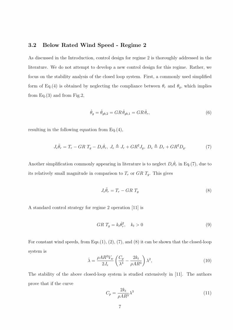
The stability of the above closed-loop system is studied extensively in [11]. The authors

prove that if the curve

Cp =2kt

ρAR3λ3 (11)

7

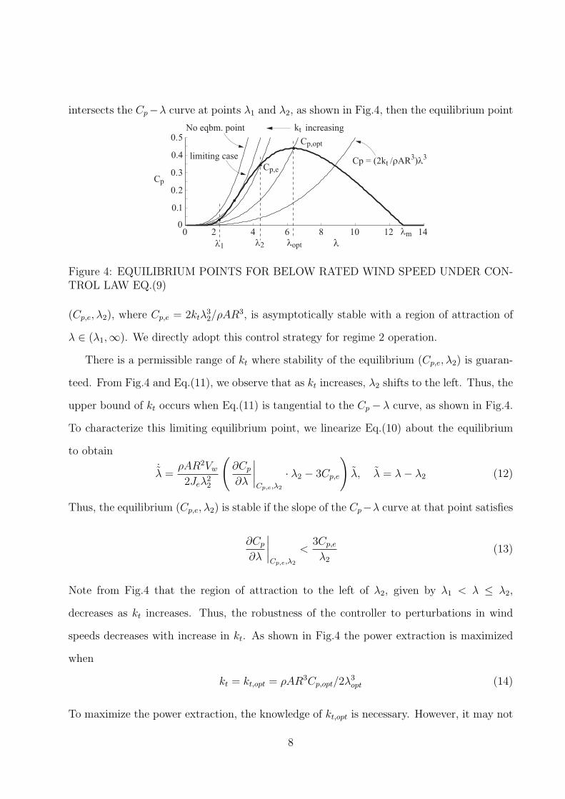
intersects the Cp−λ curve at points λ1 and λ2, as shown in Fig.4, then the equilibrium point

0 2 4 6 8 10 12 140

0.1

0.2

0.3

0.4

0.5

λ

Cp

Cp = (2kt /ρAR3)λ3

kt increasing

Cp,opt

λoptλ2λ1

Cp,e

No eqbm. point

limiting case

λm

Figure 4: EQUILIBRIUM POINTS FOR BELOW RATED WIND SPEED UNDER CON-TROL LAW EQ.(9)

(Cp,e, λ2), where Cp,e = 2ktλ32/ρAR

3, is asymptotically stable with a region of attraction of

λ ∈ (λ1,∞). We directly adopt this control strategy for regime 2 operation.

There is a permissible range of kt where stability of the equilibrium (Cp,e, λ2) is guaran-

teed. From Fig.4 and Eq.(11), we observe that as kt increases, λ2 shifts to the left. Thus, the

upper bound of kt occurs when Eq.(11) is tangential to the Cp − λ curve, as shown in Fig.4.

To characterize this limiting equilibrium point, we linearize Eq.(10) about the equilibrium

to obtain

˙̃λ =ρAR2Vw

2Jeλ22

(∂Cp

∂λ

∣∣∣∣Cp,e,λ2

· λ2 − 3Cp,e

)λ̃, λ̃ = λ− λ2 (12)

Thus, the equilibrium (Cp,e, λ2) is stable if the slope of the Cp−λ curve at that point satisfies

∂Cp

∂λ

∣∣∣∣Cp,e,λ2

<3Cp,e

λ2

(13)

Note from Fig.4 that the region of attraction to the left of λ2, given by λ1 < λ ≤ λ2,

decreases as kt increases. Thus, the robustness of the controller to perturbations in wind

speeds decreases with increase in kt. As shown in Fig.4 the power extraction is maximized

when

kt = kt,opt = ρAR3Cp,opt/2λ3opt (14)

To maximize the power extraction, the knowledge of kt,opt is necessary. However, it may not

8

be known exactly and may also change with time due to blade erosion, residue buildup etc.

Online estimation of kt,opt for power maximization has been addressed in many works such

as [11, 10, 5, 8], and is not a focus of this paper.

3.3 Above Rated Wind Speed - Regime 3

The primary control objective in regime 3 is to deliver a constant rated power, Pref . We

propose the following control law and investigate the stability of the resulting closed-loop

system obtained from Eq.(8).

Tg = Pref/θ̇rGR (15)

The resulting closed-loop equation is

Jeθ̈r = Tr − Pref/θ̇r (16)

For constant wind speed operation, as in regime 2, from Eq.(2) we have λ̇ = Rθ̈r/Vw. Since

Tr = P/θ̇r, where P is expressed in Eq.(1), we have

λ̇ =RV 2

w

Jeθ̇r

[1

2ρACp −

Pref

V 3w

](17)

For a constant Vw, the equilibrium condition is

1

2ρACp (λe) =

1

2ρACp,e =

Pref

V 3w

(18)

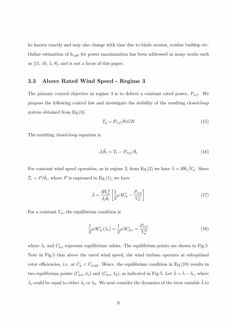
where λe and Cp,e represent equilibrium values. The equilibrium points are shown in Fig.5.

Note in Fig.5 that above the rated wind speed, the wind turbine operates at suboptimal

rotor efficiencies, i.e. at Cp < Cp,opt. Hence, the equilibrium condition in Eq.(18) results in

two equilibrium points (Cp,e, λ1) and (Cp,e, λ2), as indicated in Fig.5. Let λ̃ = λ− λe, where

λe could be equal to either λ1 or λ2. We next consider the dynamics of the error variable λ̃ to

9

0 2 4 6 8 10 12 140

0.1

0.2

0.3

0.4

0.5

λ

Cp

Cp,opt ( > Cp,e )

λoptλe = λ1

Cp,e

λe = λ2

Cp,e = 2Pref /ρAV3w

Unstable eqbm.

Stable eqbm.

λ~

Cp(λ2 + λ)~

λm

Figure 5: EQUILIBRIUM POINTS FOR ABOVE RATED WIND SPEED UNDER CON-TROL LAW EQ.(15)

investigate the stability property of the aforementioned equilibrium points. From Eqs.(17)

and (18), we obtain

˙̃λ =1

2ρA

RV 2w

Jeθ̇r

[Cp(λe + λ̃)− Cp(λe)

](19)

In Eq.(19), consider the term[Cp(λe + λ̃)− Cp(λe)

]. Note from Fig.5 that at the equilibrium

point (Cp,e, λ1),

[Cp(λ1 + λ̃)− Cp(λ1)

] > 0 when 0 < λ̃ < (λ2 − λ1)

< 0 when λ̃ < 0(20)

and at the equilibrium point (Cp,e, λ2),

[Cp(λ2 + λ̃)− Cp(λ2)

] < 0 when λ̃ > 0

> 0 when (λ1 − λ2) < λ̃ < 0(21)

Next, considering the following Lyapunov function candidate and its corresponding derivative

along systems trajectories,

V =1

2λ̃2, V̇ =

1

2ρA

RV 2w

Jeθ̇r

[Cp(λe + λ̃)− Cp(λe)

]λ̃ (22)

10

we observe that for the equilibrium point (Cp,e, λ1), V̇ > 0 for any λ̃ ̸= 0 satisfying λ̃ ∈

(−λ1, λ2 − λ1). Hence from Chetaev’s Theorem [13], we conclude that (Cp,e, λ1) is an unstable

equilibrium. For (Cp,e, λ2), however, V̇ < 0 for any λ̃ ̸= 0 satisfying λ̃ ∈ (λ1 − λ2,∞). Hence,

(Cp,e, λ2) is a locally asymptotically stable equilibrium point. Further, for the asymptotically

stable equilibrium point (Cp,e, λ2), from the observation above regarding V̇ and noting that

λ̃ moves monotonically toward 0 from either side, we conclude that the domain of attraction

is λ ∈ (λ1,∞). We note that the proposed design does not consider blade pitch variation for

attenuating generator torque variations. This will be an area of future research. We end this

section by noting that in regime 3, under the proposed controller, stable equilibrium points

lie on the Cp − λ curve where λm > λ2 > λopt and 0 < Cp,e < Cp,opt.

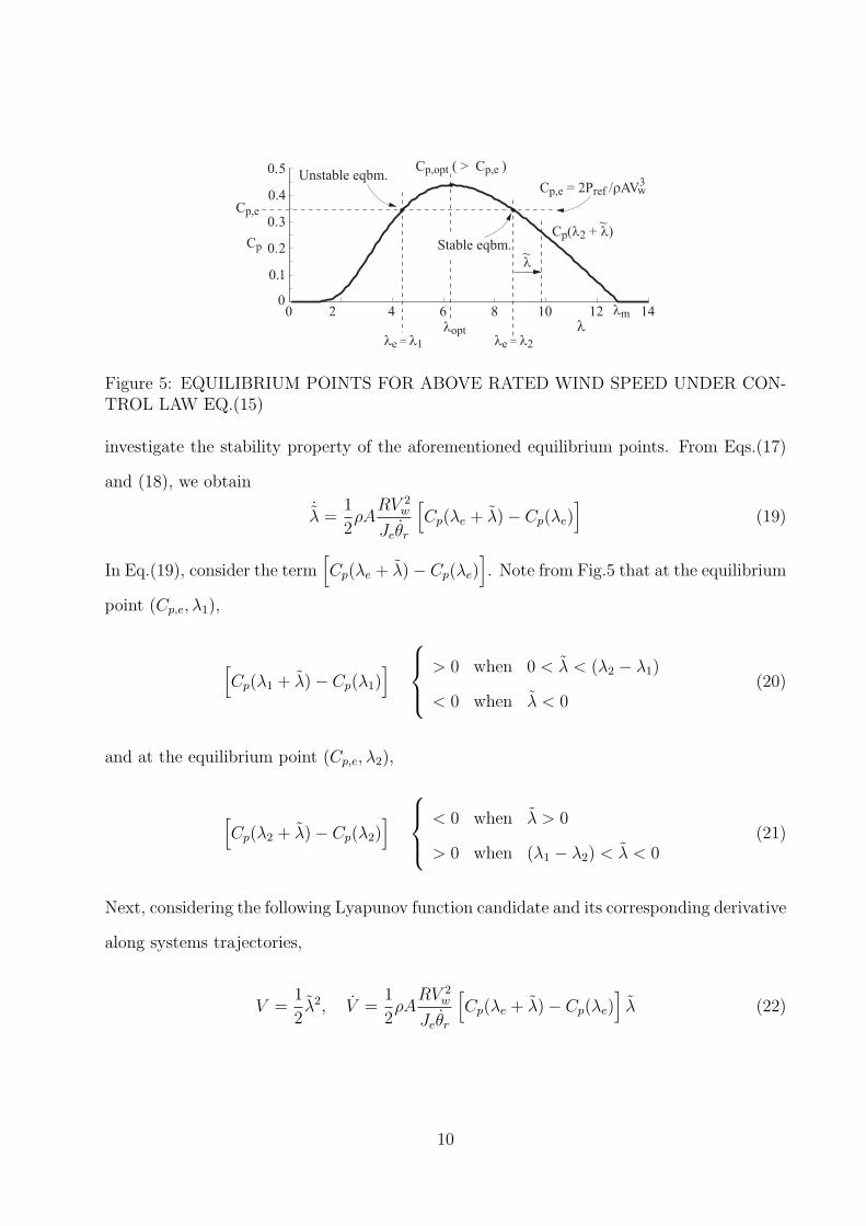
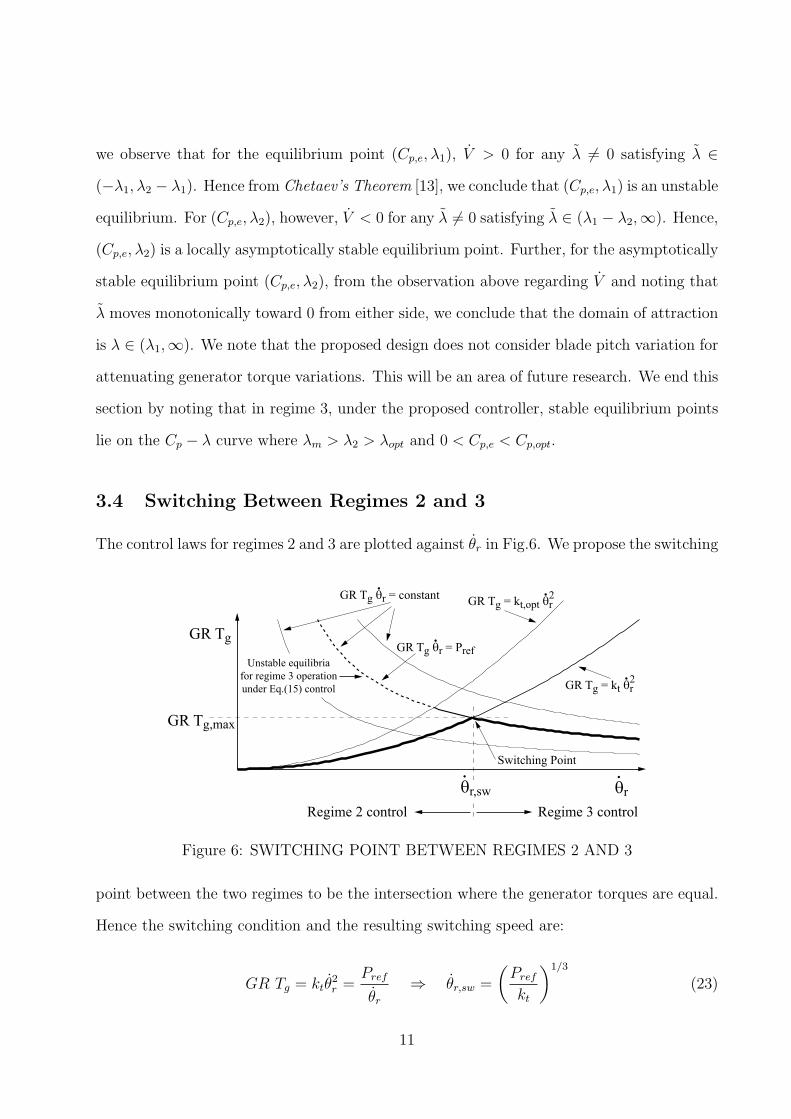
3.4 Switching Between Regimes 2 and 3

The control laws for regimes 2 and 3 are plotted against θ̇r in Fig.6. We propose the switching

θr

.

GR Tg

GR Tg θr = constant.

GR Tg = kt θr

.2

θr,sw

.

Regime 3 controlRegime 2 control

Switching Point

GR Tg,max

GR Tg θr = Pref

.

GR Tg = kt,opt θr

.2

Unstable equilibria

for regime 3 operation

under Eq.(15) control

Figure 6: SWITCHING POINT BETWEEN REGIMES 2 AND 3

point between the two regimes to be the intersection where the generator torques are equal.

Hence the switching condition and the resulting switching speed are:

GR Tg = ktθ̇2r =

Pref

θ̇r⇒ θ̇r,sw =

(Pref

kt

)1/3

(23)

11

Also, note that the control switching point corresponds to the maximum generator torque,

Tg,max. One method to determine θ̇r,sw and Pref is to use a prescribed Tg,max and a regime

2 operating point (Cp,e, λ2). Then, kt is obtained from Eq.(11) and substituting Tg,max and

kt in Eq.(23), yields

θ̇r,sw =

(GR Tg,max

kt

)1/2

⇒ Pref = ktθ̇3r,sw (24)

Alternately, knowing the rated power Pref and kt, one can determine θ̇r,sw and maximum

generator torque Tg,max using Eq.(23). Also, note that at the rated wind speed Vw,rated, the

system operates at the switching point θ̇r,sw. Therefore, from the regime 2 operating point

(Cp,e, λ2) and the rated power Pref , Vw,rated can be determined using Eq.(1) as follows

Vw,rated =

(2Pref

ρACp,e

)1/3

(25)

4 Analytical Study of the Switching Control

4.1 Common Equilibrium for Operation at Switching Point

In this section we establish that regime 2 and 3 controllers result in a common equlibrium

when the wind turbine is at equilibrium at the switching point. Here equilibrium refers to a

point on the Cp − λ curve. This is important because we wish to determine the entire set of

equilibrium points spanned by the wind turbine in regimes 2 and 3. This, in turn, will lead

to a common region of attraction for the proposed switching controller.

We first note that when the closed-loop system is at equilibrium at the switching point,

then the equilibrium rotor speed is θ̇r,sw, given by Eq.(23). Substituting for Pref from Eq.(23)

into the equilibrium condition for regime 3 in Eq.(18), we obtain

Cp,e =2kt

ρAR3λ3e (26)

12

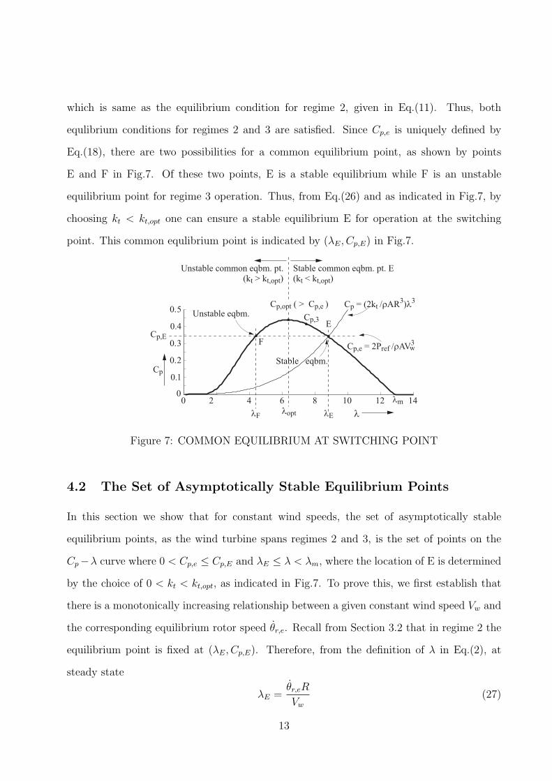
which is same as the equilibrium condition for regime 2, given in Eq.(11). Thus, both

equlibrium conditions for regimes 2 and 3 are satisfied. Since Cp,e is uniquely defined by

Eq.(18), there are two possibilities for a common equilibrium point, as shown by points

E and F in Fig.7. Of these two points, E is a stable equilibrium while F is an unstable

equilibrium point for regime 3 operation. Thus, from Eq.(26) and as indicated in Fig.7, by

choosing kt < kt,opt one can ensure a stable equilibrium E for operation at the switching

point. This common equlibrium point is indicated by (λE, Cp,E) in Fig.7.

0 2 4 6 8 10 12 140

0.1

0.2

0.3

0.4

0.5

λ

Cp

Cp = (2kt /ρAR3)λ3

λopt

Cp,opt ( > Cp,e )

Cp,E

λE

Cp,e = 2Pref /ρAV3w

Unstable eqbm.

Stable eqbm.

Stable common eqbm. pt. EUnstable common eqbm. pt.(kt < kt,opt)(kt > kt,opt)

E

F

Cp,3

λF

λm

Figure 7: COMMON EQUILIBRIUM AT SWITCHING POINT

4.2 The Set of Asymptotically Stable Equilibrium Points

In this section we show that for constant wind speeds, the set of asymptotically stable

equilibrium points, as the wind turbine spans regimes 2 and 3, is the set of points on the

Cp−λ curve where 0 < Cp,e ≤ Cp,E and λE ≤ λ < λm, where the location of E is determined

by the choice of 0 < kt < kt,opt, as indicated in Fig.7. To prove this, we first establish that

there is a monotonically increasing relationship between a given constant wind speed Vw and

the corresponding equilibrium rotor speed θ̇r,e. Recall from Section 3.2 that in regime 2 the

equilibrium point is fixed at (λE, Cp,E). Therefore, from the definition of λ in Eq.(2), at

steady state

λE =θ̇r,eR

Vw

(27)

13

Thus, from Eq.(27) we conclude that there is a monotonically increasing relationship between

Vw and θ̇r,e at steady state in regime 2. In regime 3, the equilibrium condition is given by

Eq.(18). Here, if Vw increases, Cp,e must decrease. Referring to Fig.5, we see that for stable

equilibrium points if Cp,e decreases, λe must increase and therefore θ̇r,e increases. Therefore,

there is a monotonically increasing relationship between the steady-state values of Vw and

θ̇r,e in regime 3 as well.

In Section 4.1, we have shown that regime 2 and 3 share a common stable equilibrium

(point E in Fig.7) at the point of switching. At the switching point, there exists a unique

θ̇r,e = θ̇r,sw, given by Eq.(23) or Eq.(24), and therefore a unique Vw = Vw,sw = θ̇r,swR/λE.

It can be verified using Eq.(25) that Vw,sw = Vw,rated. Therefore, we conclude from the

deductions above that for any constant Vw, there is a unique equilibrium rotor speed θ̇r,e.

Now consider the monotonically increasing behavior of Vw and θ̇r,e described above and

let there be a valid equilibrium point Cp,3 such that Cp,3 > Cp,E as shown in Fig.7. Since

regime 2 has a fixed operating point (λE, Cp,E), the operating point Cp,3 must be a regime

3 operating point. However, for regime 3 operation, Cp,3 > Cp,E implies Vw,3 < Vw,sw

according to Eq.(18), which in turn implies θ̇r,3 < θ̇r,sw from the monotonically increasing

nature of θ̇r,e with respect to Vw. This implies from Fig.6 that the equilibrium (λ3, Cp,3)

lies in regime 2, which is a contradiction. Therefore, any equilibrium point Cp,3 > Cp,E

is invalid. Furthermore, we have already shown in section 3.3 that any equilibrium point

λ ≤ λopt would be an unstable equilibrium in regime 3 operation. This proves the claim

made in this section.

4.3 Common Region of Attraction

In Section 4.2 we have established a set of asymptotically stable equilibrium points 0 <

Cp,e ≤ Cp,E spanning the operation of regimes 2 and 3. In regime 2, the region of attraction

is (λ1,∞), as indicated in Fig.4. This is a fixed region of attraction since the equilibrium

point is static at (Cp,e, λ2) = (Cp,E, λE). In regime 3, the equilibrium point is dependent on

14

wind speed Vw and for a given constant Vw, the region of attraction is (λ1,∞) as indicated in

Fig.5. Since, we have developed our analysis for constant Vw, this automatically motivates

the question of stability of the closed loop system for step changes in Vw. Step changes in

Vw can be considered as idealized wind gusts with disconitnuous increase or decrease of wind

speeds. They cause jumps in the instantaneous value of λ, and that could potentially cause

instability. They could also trigger transition between regimes and discontinuous jumps in

the equilibrium point. Hence, the stability properties of the proposed switched control would

be interesting to investigate for idealzed wind gusts. To this end, we propose and prove the

following theorem:

Theorem 1. For any step change in Vw, the set of asymptotically stable equilibrium points

on the Cp − λ curve, given by 0 < Cp ≤ Cp,E and λE ≤ λ < λm, have a common region of

attraction λF < λ < ∞ under the control laws for regimes 2 and 3, given in sections 3.2 and

3.3, and the switching criterion given in section 3.4.

Proof. As we have shown in Section 3.2 and Fig.4, the region of attraction in regime 2

is R1 = (λ1,∞). Similarly, we have shown in Section 3.3 and Fig.5 that the region of

attraction of an equilibrium (Cp,e, λ2) in regime 3 is (λ1,∞). Therefore, for a chosen regime

2 operating point E, the intersection of the regions of attraction of the set of all asymtotically

stable equilibrium points is Rc = (λF ,∞). Notably, Rc also represents a common region of

attraction of the switched system under step canges in Vw for any equilibrium point (Cp,e, λe)

satisfying 0 < Cp ≤ Cp,E and λE ≤ λ < λm. This is because λ increases monotonically when

λF < λ < λe and decreases monotonically when λ > λe in both regimes 2 and 3. Thus, from

this observation we can say that the common region of attraction Rc is (λF ,∞). We end the

proof by noting that this represents a conservative estimate of the region of attraction.

4.4 Predicting Instability Induced by Wind Gusts

In this section we explore the possibility of instability induced by indealized wind gusts

while the wind turbine operates in regimes 2 or 3. To predict instability conservatively, our

15

approach is to predict the magnitude of wind gusts that can drive λ outside (λF ,∞). It

is evident that this is only possible through step up in Vw and not through step down in

Vw. Suppose that the wind turbine is operating at steady state at the stable equilibrium

point with a wind speed of Vw,i and a tip speed ratio of λi. Let us assume a ideal wind gust

∆Vw which instantaneously increases the wind speed to Vw,f = Vw,i +∆Vw. Consequently, λ

incurs an instantaneous change to λf . Thus,

λi =θ̇RR

Vw,i

λf =θ̇RR

Vw,f

(28)

Since the system was at equilibrium just prior to the wind gust, and due to the large inertia

associated with θ̇R, θ̇R remains unchanged at the instant of the wind gust. Conservatively,

instability is induced if λf ≤ λF . Thus ∆Vw that can cause instability is

∆Vw = Vw,f − Vw,i >

(λi

λF

− 1

)Vw,i (29)

This estimate is conservative because in regime 2, the region of attraction is much larger

than (λF ,∞) and in regime 3, the minimum region of attraction is (λF ,∞) corresponding

to operation at Vw,sw and it increase as Vw increases.

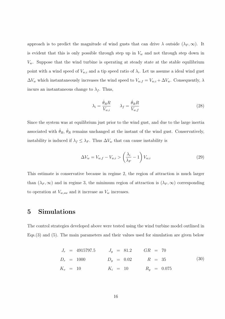
5 Simulations

The control strategies developed above were tested using the wind turbine model outlined in

Eqs.(3) and (5). The main parameters and their values used for simulation are given below

Jr = 4915797.5 Jg = 81.2 GR = 70

Dr = 1000 Dg = 0.02 R = 35

Kv = 10 Ki = 10 Rg = 0.075

(30)

16

The parameter values for Jr, Jg, GR and R were obtained from [15] for a 1.5MW wind

turbine. The rest were estimated. In particular, the parameters Kv and Ki were chosen to

approximately obtain the rated current and voltages reported in [15]. The parameter Rg was

chosen to yield a generator efficiency of ≈ 95 − 98% at the rated power [9]. The Cp(β, λ)

surface was modeled as the following function

Cp (β, λ) = 0.22(

116λi

− 0.4β − 5)e− 12.5

λi

1λi

= 1λ+0.08β

− 0.035β3+1

(31)

The surface represented by Eq.(31) is plotted in Fig.1. The calculation of Cp requires blade

element theory and Eq.(31) is an approximate analytical solution [6, 16]. The control laws

designed in this paper do not assume knowledge of the surface.

In designing the control switching point θ̇r,sw, we consider the pitch angle to be fixed at

β = 0. Note that for the chosen system, Cp,opt = 0.43821 and λopt = 6.325. Thus, from

Eq.(14), we have kt,opt = 1.7502× 105. The value of kt is chosen as kt = 1.5× 105 for simula-

tions, which will lead to suboptimal power extraction in regime 2. For power maximization,

one of the existing methods for estimating kt,opt, such as [11], could be augmented to the

basic control in Eq.(9). Thus, from Eq.(23)

Pref = 1.5× 106 W, kt = 1.5× 105 ⇒ θ̇r,sw = 2.1544 rad/s (32)

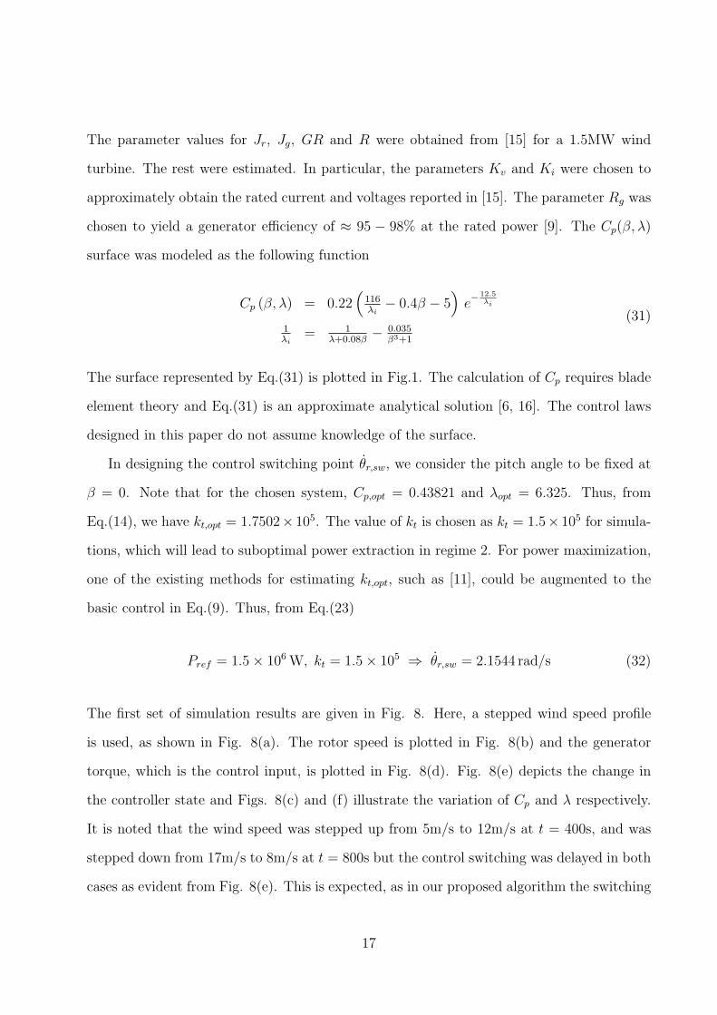
The first set of simulation results are given in Fig. 8. Here, a stepped wind speed profile

is used, as shown in Fig. 8(a). The rotor speed is plotted in Fig. 8(b) and the generator

torque, which is the control input, is plotted in Fig. 8(d). Fig. 8(e) depicts the change in

the controller state and Figs. 8(c) and (f) illustrate the variation of Cp and λ respectively.

It is noted that the wind speed was stepped up from 5m/s to 12m/s at t = 400s, and was

stepped down from 17m/s to 8m/s at t = 800s but the control switching was delayed in both

cases as evident from Fig. 8(e). This is expected, as in our proposed algorithm the switching

17

0 200 400 600 800 10005

10

15

20

00.10.20.30.40.5

0

4

8

12

05

10152025

0

2

4

6

0 200 400 600 800 1000 0 200 400 600 800 1000

0 200 400 600 800 1000 0 200 400 600 800 1000 0 200 400 600 800 1000

time (s) time (s) time (s)

X 103

Co

ntr

oll

er

Sta

te

Cp

λ

Regime 3

Regime 2

Tg

(N

m)

Vw

(m

/s)

θr

(rad

/s)

.

(a) (b) (c)

(d) (e) (f)

Figure 8: RESPONSE OF WIND TURBINE TO STEP CHANGES IN WIND SPEED

is governed by θ̇r. It is also confirmed from Figs. 8(c) and (f) that the equilibrium the point

Cpe , λe takes a fixed value independent of wind speed in regime 2, while it is dependent on

the wind speed in regime 3. Also note that there is no discontinuity the control input Tg at

the switching points. Finally, Fig. 8(f) also shows that transient λ varies monotonically in

approaching equilibrium in both regimes 2 and 3, justifying the common region of attraction

claimed in section 4.3. It is interesting to observe that the stepping down of wind speed at

800s caused a significant instantaneous jump in λ to λ > λm, causing Cp = 0 for a finite

duration. Nevertheless, the regime 2 equilibrium point (Cp,E, λE) was attained since it has a

region of attraction λF < λ < ∞. The power extraction and associated losses will be shown

in the following simulation results.

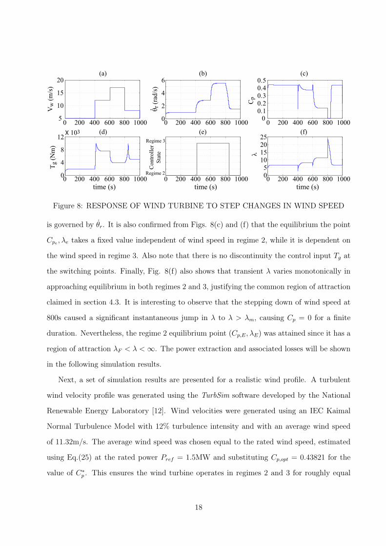
Next, a set of simulation results are presented for a realistic wind profile. A turbulent

wind velocity profile was generated using the TurbSim software developed by the National

Renewable Energy Laboratory [12]. Wind velocities were generated using an IEC Kaimal

Normal Turbulence Model with 12% turbulence intensity and with an average wind speed

of 11.32m/s. The average wind speed was chosen equal to the rated wind speed, estimated

using Eq.(25) at the rated power Pref = 1.5MW and substituting Cp,opt = 0.43821 for the

value of C∗p . This ensures the wind turbine operates in regimes 2 and 3 for roughly equal

18

0 200 400 600 800 10006

8

10

12

14

16

18

time (s)

Vw

(m

/s)

Figure 9: WIND SPEED PROFILE USED FOR SIMULATIONS

amounts of time over the duration of simulation. The generated wind speed data is shown

in Fig.9.

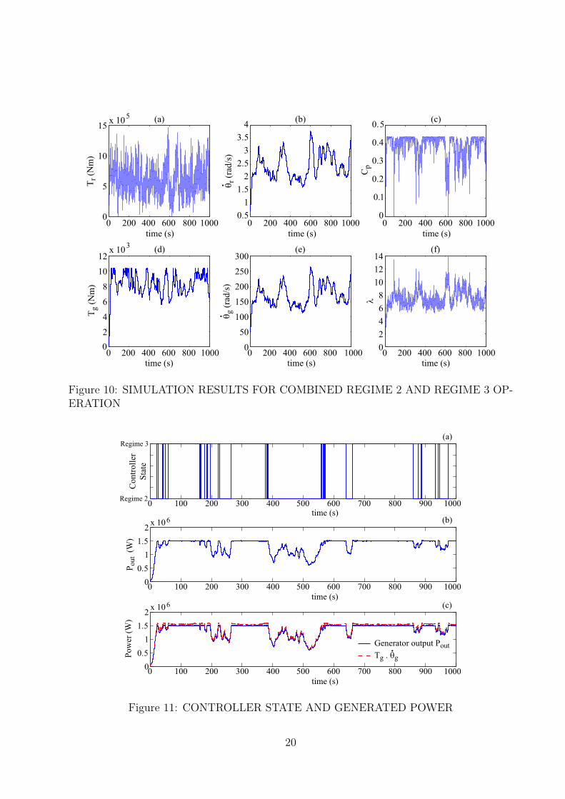
The simulation results are shown in Figs.10 and 11. In this simulation, the regime 3

control torque Tg was designed as

Tg = (Pref + Ploss) /θ̇rGR (33)

instead of Eq.(15), to account for electrical losses. The term Ploss = i2gRg, according to our

simplified generator model in Eq.(5). Equation (33) assumes the electrical power losses to

be known. Figs.10(a), (b), (d) and (e) show the variations in Tr, θ̇r, Tg and θ̇g, respectively.

Note that Tg is upper bounded due to the control design. The bound can be estimated

from Eq.(24) to be Tg,max ≈ 10kNm, which matches with that in Fig.10(d). The Cp and λ

plots are given in Figs.10(c) and (f) respectively. The plots show that λ primarily remains

confined to the region λ ≥ λopt with small transient excursions to λ < λopt. The former

region contains the set of stable equilibria for both regimes 2 and 3. In Fig.11(a), we plot

the controller state that switches between regimes 2 and 3. In Fig.11(b) we plot the generated

power. Comparing Figs.11(a) and (b), we confirm that indeed in regime 3, the rated power

is maintained at 1.5MW. Also, from Fig.10(d) and Fig.11(a) we note that there is not abrupt

19

0 200 400 600 800 10000

5

10

15x 10

5

0 200 400 600 800 10000.5

1

1.5

2

2.5

3

3.5

4

0 200 400 600 800 10000

0.1

0.2

0.3

0.4

0.5

0 200 400 600 800 10000

2

4

6

8

10

12

0 200 400 600 800 10000

50

100

150

200

250

300

0 200 400 600 800 10000

2

4

6

8

10

12

14x 10

3

time (s) time (s) time (s)

(a) (b) (c)

(d) (e) (f)

time (s) time (s) time (s)

Tr

(Nm

)T

g (

Nm

)

θr

(rad

/s)

.θ

g (

rad/s

).

Cp

λ

Figure 10: SIMULATION RESULTS FOR COMBINED REGIME 2 AND REGIME 3 OP-ERATION

0 100 200 300 400 500 600 700 800 900 1000

0 100 200 300 400 500 600 700 800 900 10000

0.5

1

1.5

2x 106

0 100 200 300 400 500 600 700 800 900 10000

0.5

1

1.5

2x 106

Po

ut (

W)

Contr

oll

er

Sta

te

Regime 3

Regime 2

Pow

er (

W)

Generator output Pout

Tg . θg

time (s)

time (s)

time (s)

(a)

(c)

(b)

.

Figure 11: CONTROLLER STATE AND GENERATED POWER

20

switching of the control input Tg at switching points, as ensured by the control design. In

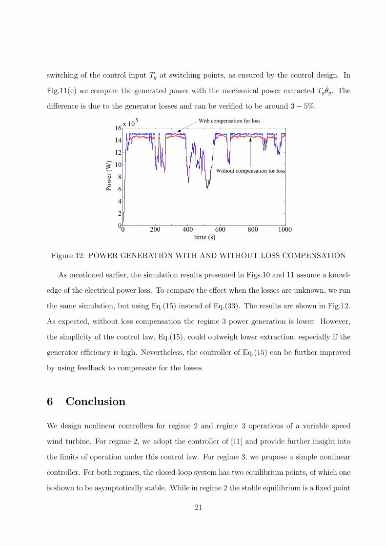
Fig.11(c) we compare the generated power with the mechanical power extracted Tgθ̇g. The

difference is due to the generator losses and can be verified to be around 3− 5%.

0 200 400 600 800 10000

2

4

6

8

10

12

14

16x 10

5

time (s)

Pow

er (

W)

With compensation for loss

Without compensation for loss

Figure 12: POWER GENERATION WITH AND WITHOUT LOSS COMPENSATION

As mentioned earlier, the simulation results presented in Figs.10 and 11 assume a knowl-

edge of the electrical power loss. To compare the effect when the losses are unknown, we run

the same simulation, but using Eq.(15) instead of Eq.(33). The results are shown in Fig.12.

As expected, without loss compensation the regime 3 power generation is lower. However,

the simplicity of the control law, Eq.(15), could outweigh lower extraction, especially if the

generator efficiency is high. Nevertheless, the controller of Eq.(15) can be further improved

by using feedback to compensate for the losses.

6 Conclusion

We design nonlinear controllers for regime 2 and regime 3 operations of a variable speed

wind turbine. For regime 2, we adopt the controller of [11] and provide further insight into

the limits of operation under this control law. For regime 3, we propose a simple nonlinear

controller. For both regimes, the closed-loop system has two equilibrium points, of which one

is shown to be asymptotically stable. While in regime 2 the stable equilibrium is a fixed point

21

on the (Cp, λ) curve, in regime 3 its location changes with wind speed. Switching between the

two regimes is based on the rotor speed whose measurement is assumed available. The control

input maintains continuity at the switching point. An analytical study of the switching

control yields a common region of attraction of the set of stable equilibrium points under step

changes in wind speeds. The controllers and the switching mechanism are validated through

simulations. The work presented in this paper can be further improved by incorporating

blade pitch modulation in regime 3 to reduce transients in generator torques. This feature

can potentially be augmented to the proposed regime 3 controller.

References

[1] B. Boukhezzar, L. Lupu, H. Siguerdidjane, and M. Hand. Multivariable control strategy

for variable speed, variable pitch wind turbines. Renewable, 32:1273–1287, 2007.

[2] B. Boukhezzar and H. Siguerdidjane. Nonlinear control of variable speed wind turbines

for power regulation. Proceedings of the IEEE Conference on Control Applications,

pages 114–119, Toronto, Canada, August 2005.

[3] B. Boukhezzar, H. Siguerdidjane, and M. Hand. Nonlinear control of variable-speed

wind turbines for generator torque limiting and power optimization. ASME Journal of

Solar Energy Engineering, 128:516–530, 2006.

[4] T. Burton, D. Sharpe, N. Jenkins, and E. Bossanyi. Wind Energy Handbook. Wiley, 1st

edition, 2001.

[5] J. Creaby, Y. Li, and J. E. Seem. Maximizing wind turbine energy capture using multi-

variable extremum seeking control. Wind Engineering, 33(4):361–387, June, 2009.

[6] F. Gao, D. Xu, and Y. Lv. Pitch-control for large-scale wind turbines based on feed

forward fuzzy-PI. Proceedings of the 7th World Congress on Intelligent Control and

Automation, June 25-27, Chongqing, China, pages 2277–2282, 2008.

22

[7] J. F. Hall, C. A. Mecklenborg, D. Chen, and S. B. Pratap. Wind energy conversion with

a variable-ratio gearbox: design and analysis. Renewable Energy, 36:1075–1080, 2011.

[8] T. Hawkins, W. N. White, G. Hu, and F. D. Sahneh. Wind turbine power capture control

with robust estimation. Proceedings of ASME 2010 Dynamic Systems and Control

Conference, September 12-15, 2010.

[9] B. K. Hodge. Alternative Energy Systems and Applications. John Wiley & Sons, Inc.,

2009.

[10] E. Iyasere, M. Salah, D. Dawson, and J. Wagner. Nonlinear robust control to maximize

energy capture in a variable speed wind turbine. American Control Conference, Seattle,

Washington, pages 1824–1829, June 11-13, 2008.

[11] K. E. Johnson, L. Y. Pao, M. J. Ballas, and L. J. Fingersh. Control of variable-speed

wind turbines. IEEE Control Systems Magazine, pages 70–81, June, 2006.

[12] N. Kelley and B. Jonkman. NWTC design codes.

http://wind.nrel.gov/designcodes/preprocessors/turbsim/, 2011.

[13] H. Khalil. Nonlinear Systems. Prentice-Hall, Inc. Upper Saddle River, NJ, 3 edition,

2002.

[14] W. E. Leithead and B. Connor. Control of variable speed wind turbines: Design task.

International Journal of Control, 73(13):1189–1212, 2000.

[15] S. Santoso and H. T. Le. Fundamental time-domain wind turbine models for wind power

studies. Renewable Energy, 32:2436–2452, 2007.

[16] J. G. Slootweg, H. Polinder, and W. L. Kling. Dynamic modeling of a winf turbine with

doubly fed induction generator. IEEE Power Engineering Society Summer Meeting,

1:644–649, 2001.

23

[17] A. D. Wright, L. J. Fingersh, and M. J. Ballas. Testing state-space controls for the con-

trols advanced research turbine. ASME Journal of Solar Energy Engineering, 128:506–

515, November, 2006.

24