18th International Conference on Supersymmetry and Unification of Fundamental Interactions (SUSY10) Physikalisches Institut, Bonn, GERMANY 24th August, 2010 Non-supersymmetric Extremal RN-AdS Black Holes Non-supersymmetric Extremal RN-AdS Black Holes Non-supersymmetric Extremal RN-AdS Black Holes in N = 2 Gauged Supergravity in N = 2 Gauged Supergravity in N = 2 Gauged Supergravity based on arXiv:1005.4607 [hep-th] Tetsuji KIMURA (KEK, JAPAN)

Welcome message from author
This document is posted to help you gain knowledge. Please leave a comment to let me know what you think about it! Share it to your friends and learn new things together.
Transcript

18th International Conference on Supersymmetry and Unification of Fundamental Interactions (SUSY10)
Physikalisches Institut, Bonn, GERMANY
24th August, 2010
Non-supersymmetric Extremal RN-AdS Black HolesNon-supersymmetric Extremal RN-AdS Black HolesNon-supersymmetric Extremal RN-AdS Black Holes
in N = 2 Gauged Supergravityin N = 2 Gauged Supergravityin N = 2 Gauged Supergravity
based on arXiv:1005.4607 [hep-th]
Tetsuji KIMURA (KEK, JAPAN)

Introduction

Introduction
Motivation: search Black Hole solutions in 4D N = 2 Gauged SUGRA
b WHY N = 2 (8-SUSY charges)?
��� Scalar fields living in highly symmetric spaces
��� (Flux) compactification scenarios in string/M-theory
b WHY Gauged?
��� Non-trivial scalar potential giving the cosmological constant
b WHY Black Holes?
��� Attractive in the study of solutions in 4D N = 2 SUGRA
��� Application to AdS4/CFT3 (or AdS4/CMP3)
Tetsuji KIMURA : Non-SUSY Extremal RN-AdS BHs in N = 2 Gauged SUGRA - 3 -
Introduction
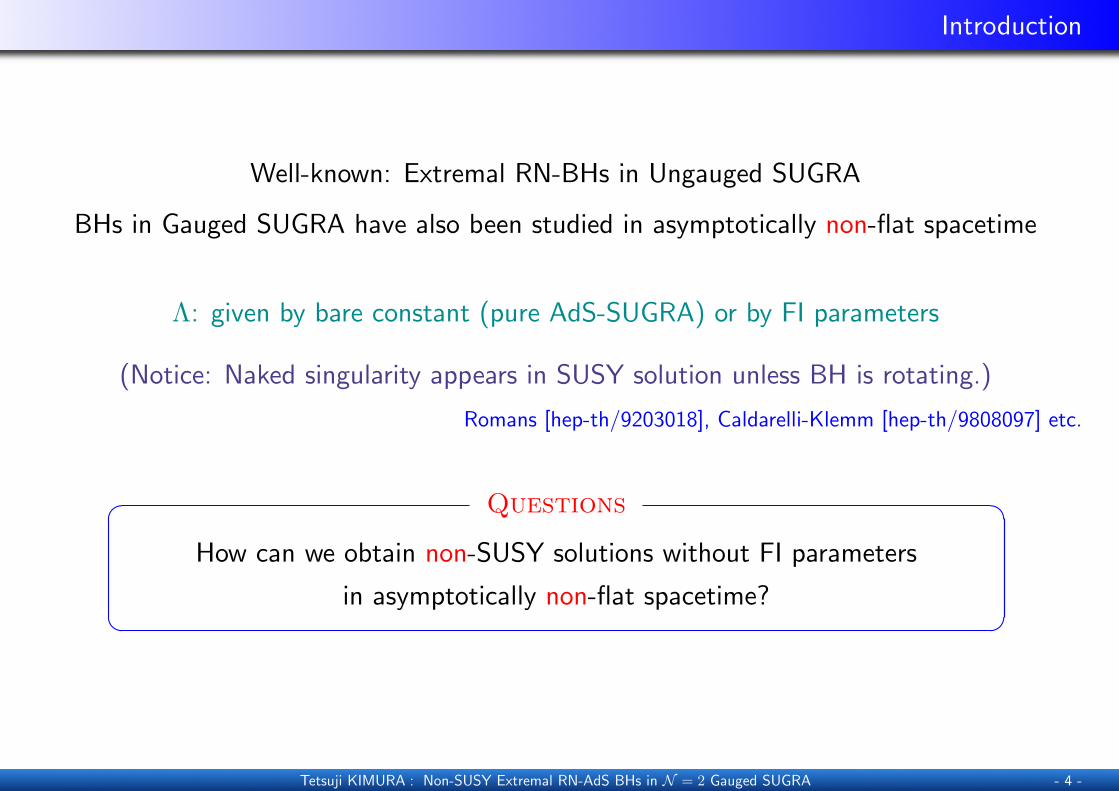
Well-known: Extremal RN-BHs in Ungauged SUGRA
BHs in Gauged SUGRA have also been studied in asymptotically non-flat spacetime
Λ: given by bare constant (pure AdS-SUGRA) or by FI parameters
(Notice: Naked singularity appears in SUSY solution unless BH is rotating.)
Romans [hep-th/9203018], Caldarelli-Klemm [hep-th/9808097] etc.
Questions� �How can we obtain non-SUSY solutions without FI parameters
in asymptotically non-flat spacetime?� �
Tetsuji KIMURA : Non-SUSY Extremal RN-AdS BHs in N = 2 Gauged SUGRA - 4 -

Contents
Introduction
N = 2 Gauged SUGRA
Effective Black Hole Potential
Attractor Equation
Single Modulus Model
Discussions
Contents
Introduction
N = 2 Gauged SUGRA
Effective Black Hole Potential
Attractor Equation
Single Modulus Model
Discussions
N = 2 Gauged SUGRA
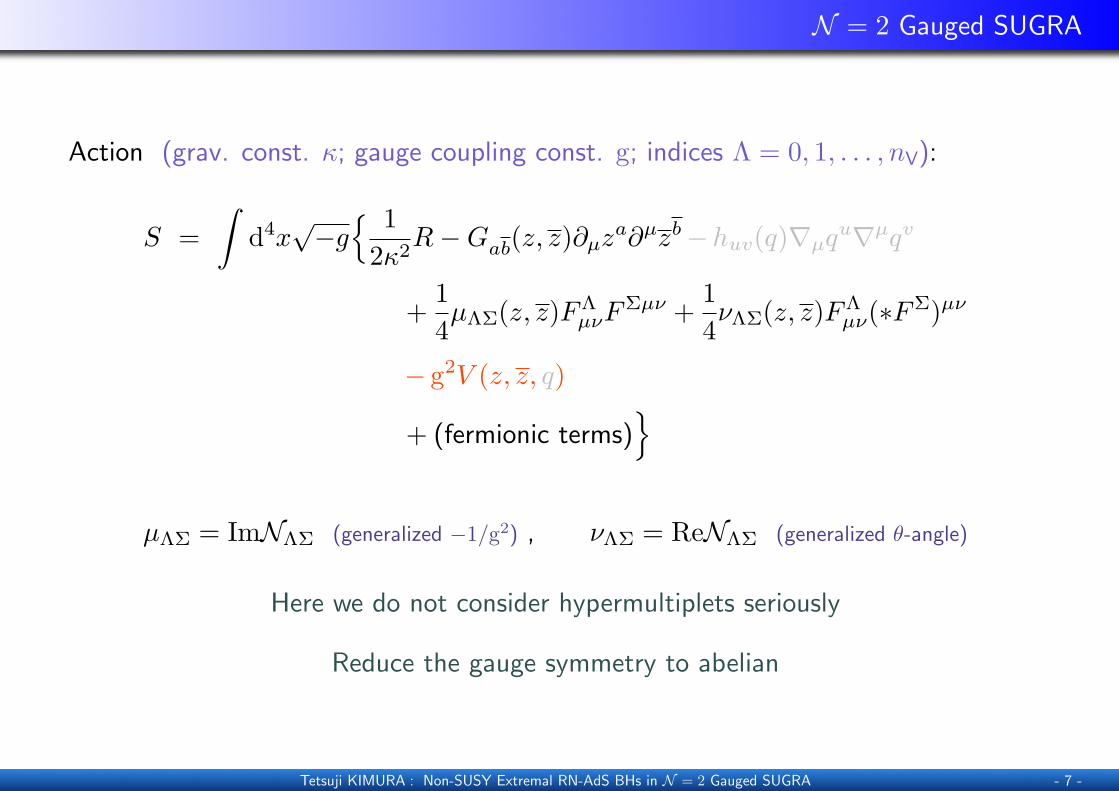
Action (grav. const. κ; gauge coupling const. g; indices Λ = 0, 1, . . . , nV):
S =∫
d4x√−g{ 1
2κ2R−Gab(z, z)∂µz
a∂µzb−huv(q)∇µqu∇µqv
+14µΛΣ(z, z)FΛ
µνFΣµν +
14νΛΣ(z, z)FΛ
µν(∗FΣ)µν
− g2V (z, z, q)
+ (fermionic terms)}
µΛΣ = ImNΛΣ (generalized −1/g2) , νΛΣ = ReNΛΣ (generalized θ-angle)
Here we do not consider hypermultiplets seriously
Reduce the gauge symmetry to abelian
Tetsuji KIMURA : Non-SUSY Extremal RN-AdS BHs in N = 2 Gauged SUGRA - 7 -

N = 2 Gauged SUGRA
Equations of Motion (abbreviate κ and g; set fermionic fields to be zero):
gµν :(Rµν −
12Rgµν
)− 2Gab ∂(µz
a∂ν)zb +Gab ∂ρz
a∂ρzb gµν = Tµν −V gµν
Tµν = −µΛΣFΛµρF
Σνσ g
ρσ +14µΛΣF
Λρσ F
Σρσ gµν (energy-momentum tensor)
za : −Gab√−g
∂µ
(√−ggµν∂νz
b)−∂Gab
∂zc∂ρz
b ∂ρzc
=14∂µΛΣ
∂zaFΛ
µνFΣµν +
14∂νΛΣ
∂zaFΛ
µν(∗FΣ)µν − ∂V
∂za
AΛµ : εµνρσ∂νGΛρσ = 0 , GΛρσ = νΛΣF
Σρσ − µΛΣ(∗FΣ)ρσ
electric charge qΛ ≡14π
∫S2GΛ , magnetic charge pΛ ≡ 1
4π
∫S2FΛ
Tetsuji KIMURA : Non-SUSY Extremal RN-AdS BHs in N = 2 Gauged SUGRA - 8 -

Metric Ansatz
Introduce a metric ansatz for RN(-AdS) BH: “charged”, “static”, “spherically symmetric”
'
&
$
%ds2 = −e2A(r)dt2 + e2B(r)dr2 + e2C(r)r2
(dθ2 + sin2 θ dφ2
)AdS2 × S2 as near horizon geometry (radii: rA and rH)
A(r) = logr − rHrA
, B(r) = −A(r) , C(r) = logrHr
R(AdS2 × S2) = 2(− 1r2A
+1r2H
)×
→ ds2(near horizon) = −(r − rHrA
)2
dt2 +(
rAr − rH
)2
dr2 + r2H(dθ2 + sin2 θ dφ2
)= −e2τ
r2Adt2 + r2Adτ2 + r2H
(dθ2 + sin2 θ dφ2
)(τ = log(r − rH))
Area of horizon is AH = 4πr2H
Tetsuji KIMURA : Non-SUSY Extremal RN-AdS BHs in N = 2 Gauged SUGRA - 9 -
Metric Ansatz
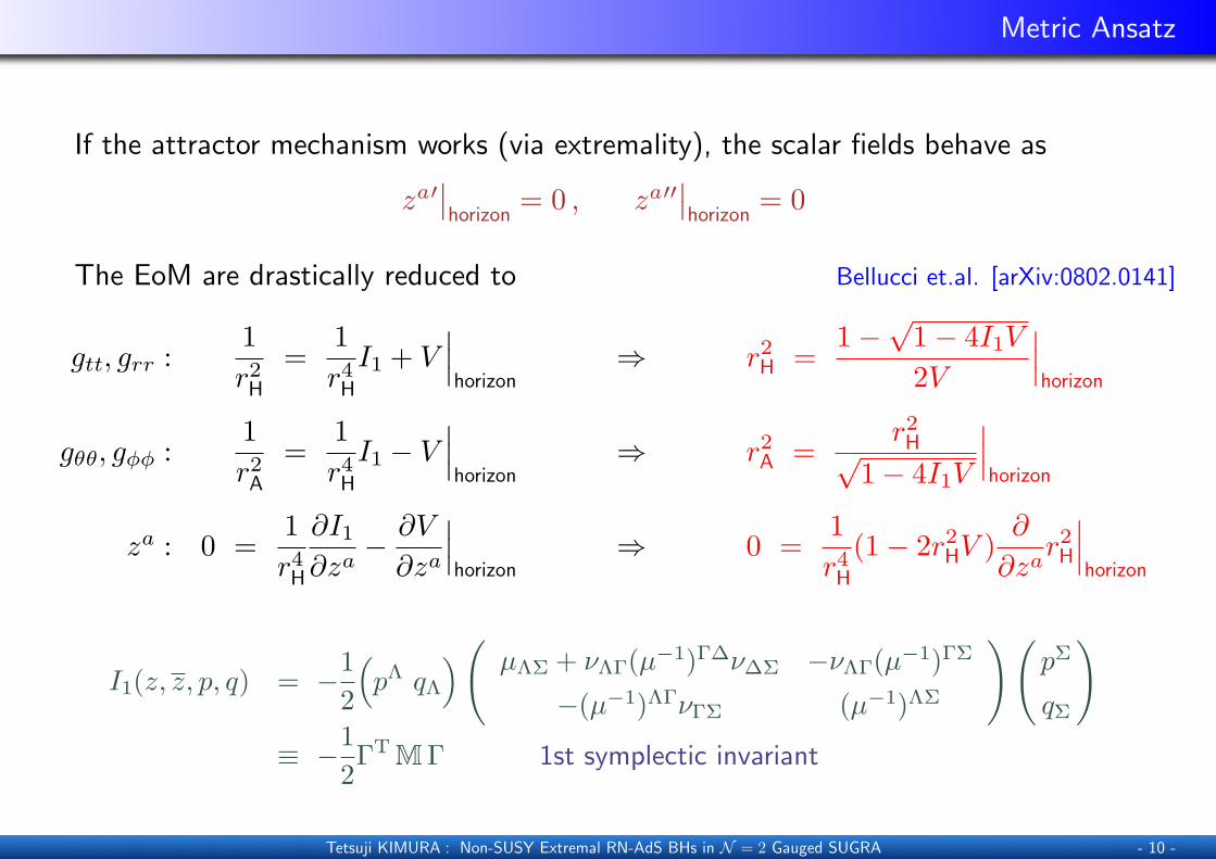
If the attractor mechanism works (via extremality), the scalar fields behave as
za′∣∣horizon
= 0 , za′′∣∣horizon
= 0
The EoM are drastically reduced to Bellucci et.al. [arXiv:0802.0141]
gtt, grr :1r2H
=1r4HI1 + V
∣∣∣horizon
⇒ r2H =1−√
1− 4I1V2V
∣∣∣horizon
gθθ, gφφ :1r2A
=1r4HI1 − V
∣∣∣horizon
⇒ r2A =r2H√
1− 4I1V
∣∣∣horizon
za : 0 =1r4H
∂I1∂za− ∂V
∂za
∣∣∣horizon
⇒ 0 =1r4H
(1− 2r2HV )∂
∂zar2H
∣∣∣horizon
I1(z, z, p, q) = −12
(pΛ qΛ
)( µΛΣ + νΛΓ(µ−1)Γ∆ν∆Σ −νΛΓ(µ−1)ΓΣ
−(µ−1)ΛΓνΓΣ (µ−1)ΛΣ
)(pΣ
qΣ
)≡ −1
2ΓT M Γ 1st symplectic invariant
Tetsuji KIMURA : Non-SUSY Extremal RN-AdS BHs in N = 2 Gauged SUGRA - 10 -

Effective Black Hole Potential
Black Hole Entropy is given as the Area of the horizon as in the case of RN-BH:
SBH(p, q) =AH
4π= r2H
∣∣∣horizon
≡ Veff(z, z, p, q)∣∣∣horizon
Veff(z, z, p, q) =1−√
1− 4I1V2V
Veff → I1 (if V → 0)
0 =1r4H
(1− 2r2HV )∂
∂zaVeff
∣∣∣horizon
We read the “cosmological constant Λ” from the scalar curvature:
R(AdS2 × S2) = 2(− 1r2A
+1r2H
)= 4V
V∣∣horizon
≡ Λ(“cosmological constant”)
The “attractor equation” which we have to solve is 0 =∂
∂zaVeff(z, z, p, q)
∣∣∣horizon
(If rH is finite and if Λ is non-positive)
Tetsuji KIMURA : Non-SUSY Extremal RN-AdS BHs in N = 2 Gauged SUGRA - 11 -

Effective Black Hole Potential
The “attractor equation” which we have to solve is
0 =∂
∂zaVeff(z, z, p, q)
∣∣∣horizon
=1
2V 2√
1− 4I1V
{2V 2∂I1
∂za−(√
1− 4I1V + 2I1V − 1)∂V∂za
} ∣∣∣∣∣horizon
Evaluate I1 and V : Description in terms of the central charge Z
Useful when we consider (non-)SUSY solutions
Def. of Z comes from the SUSY variation of gravitini:
δψAµ = DµεA + εAB T−µν γ
ν εB + igSAB γµ εB + (fermionic fields)
Z = −12
(14π
∫S2T−), SAB =
i
2(σx)ABPx
Use the property of the Special Kahler geometry
Tetsuji KIMURA : Non-SUSY Extremal RN-AdS BHs in N = 2 Gauged SUGRA - 12 -
Special Kahler Geometry
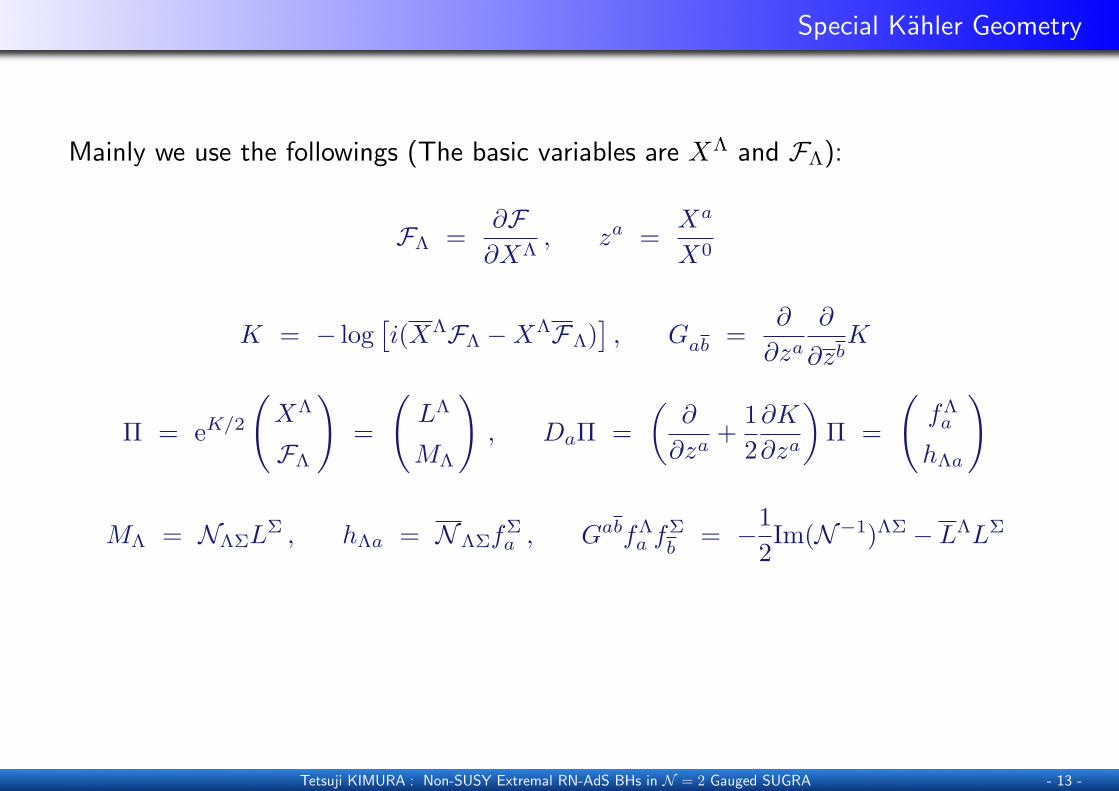
Mainly we use the followings (The basic variables are XΛ and FΛ):
FΛ =∂F∂XΛ
, za =Xa
X0
K = − log[i(XΛFΛ −XΛFΛ)
], Gab =
∂
∂za
∂
∂zbK
Π = eK/2
(XΛ
FΛ
)=
(LΛ
MΛ
), DaΠ =
(∂
∂za+
12∂K
∂za
)Π =
(fΛ
a
hΛa
)
MΛ = NΛΣLΣ , hΛa = NΛΣf
Σa , GabfΛ
a fΣb
= −12Im(N−1)ΛΣ − LΛLΣ
Tetsuji KIMURA : Non-SUSY Extremal RN-AdS BHs in N = 2 Gauged SUGRA - 13 -

Special Kahler Geometry
Write down Z, I1 and V in terms of (LΛ,MΛ) = eK/2(XΛ,FΛ):
Z = LΛ qΛ −MΛ pΛ
I1 = |Z|2 +GabDaZDbZ
V =3∑
x=1
(− 3|Px|2 +GabDaPxDbPx
)+ 4huv k
ukv
PxΛ, PxΛ: SU(2) triplet of Killing prepotentials in N = 2 SUGRA
Px = PxΛL
Λ − PxΛMΛ in SAB (x = 1, 2, 3)
If no hypermultiplets, only P3 = P3ΛL
Λ − P3ΛMΛ contributes to the potential.
Further, we could identify (P3Λ, P3Λ) = (qΛ, pΛ) P3 ≡ Z Cassani et.al. [arXiv:0911.2708]
V = −3|Z|2 +GabDaZDbZ
Tetsuji KIMURA : Non-SUSY Extremal RN-AdS BHs in N = 2 Gauged SUGRA - 14 -

Attractor Equation
Rewrite the “attractor equation” in terms of the central charge:
0 =∂
∂zaVeff(z, z, p, q)
∣∣∣horizon
=1
2V 2√
1− 4I1V
{2V 2∂I1
∂za−(√
1− 4I1V + 2I1V − 1)∂V∂za
} ∣∣∣∣∣horizon
=1 + V 2
eff√1− 4I1V
{2GVZDaZ + iCabcG
bbGccDbZ DcZ}∣∣∣∣∣
horizon
A Non-trivial factor GV =1− V 2
eff
1 + V 2eff
If Λ < 0 and DaZ = 0 (SUSY) → Naked Singularity → Search non-SUSY sol. DaZ 6= 0
If ∂aI1 = 0 or ∂aV = 0 → V |horizon = Λ = 0, or Empty Hole Z|horizon = 0
If GV = 0 → SBH = 1 (strange!)
Tetsuji KIMURA : Non-SUSY Extremal RN-AdS BHs in N = 2 Gauged SUGRA - 15 -

Attractor Equation
Rewrite the “attractor equation” in terms of the central charge:
0 =∂
∂zaVeff(z, z, p, q)
∣∣∣horizon
=1
2V 2√
1− 4I1V
{2V 2∂I1
∂za−(√
1− 4I1V + 2I1V − 1)∂V∂za
} ∣∣∣∣∣horizon
=1 + V 2
eff√1− 4I1V
{2GVZDaZ + iCabcG
bbGccDbZ DcZ}∣∣∣∣∣
horizon
Solve the equation 0 = 2GVZDaZ + iCabcGbbGccDbZ DcZ
∣∣∣horizon
under the condition V < 0, 1− 4I1V > 0, ∂aI1 6= 0, ∂aV 6= 0, DaZ 6= 0
Tetsuji KIMURA : Non-SUSY Extremal RN-AdS BHs in N = 2 Gauged SUGRA - 16 -

Contents
Introduction
N = 2 Gauged SUGRA
Effective Black Hole Potential
Attractor Equation
Single Modulus Model
Discussions

Example: D0-D4 System in T3-model
Consider the single modulus model w/ charges Γ = (0, p, 0, q0) (“D0-D4” system):
Holomorphic central charge W = e−K/2Z and its discriminant ∆(W ) are
F =(X1)3
X0, t =
X1
X0; W = q0 − 3p t2 , ∆(W ) = 12pq0
The attractor equation and its solution (t = 0 + iy, y < 0):
p(y2)3 + (q0 − 18p3q20)(y2)2 − 12p2q30(y
2)− 2pq40 = 0
y2 = A+B or A+ ω±B (ω3 = 1)
A =q03p(18p3q0 − 1
), B =
13p
(C1/3 +
q204
1 + (18p3q0)2
C1/3
)C = −q30
[1− 27p3q0 − (18p3q0)3 − 3
√3√−2p3q0 − 9(p3q0)2 − 432(p3q0)3
]
with pq0 < 0
Tetsuji KIMURA : Non-SUSY Extremal RN-AdS BHs in N = 2 Gauged SUGRA - 18 -
Example: D0-D4 System in T3-model
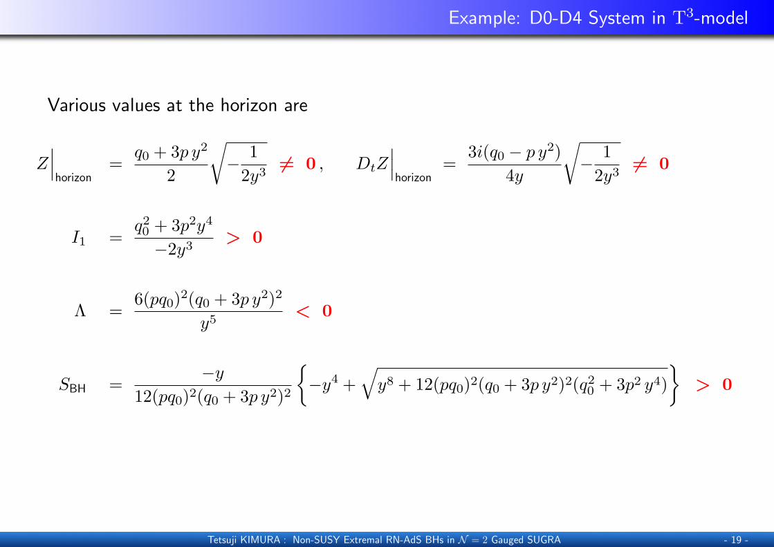
Various values at the horizon are
Z∣∣∣horizon
=q0 + 3p y2
2
√− 1
2y36= 0 , DtZ
∣∣∣horizon
=3i(q0 − p y2)
4y
√− 1
2y36= 0
I1 =q20 + 3p2y4
−2y3> 0
Λ =6(pq0)2(q0 + 3p y2)2
y5< 0
SBH =−y
12(pq0)2(q0 + 3p y2)2
{−y4 +
√y8 + 12(pq0)2(q0 + 3p y2)2(q20 + 3p2 y4)
}> 0
Tetsuji KIMURA : Non-SUSY Extremal RN-AdS BHs in N = 2 Gauged SUGRA - 19 -

Example: D0-D4 System in T3-model
Focus on the Large q0 limit:
The dominant part ot the Modulus t = 0 + iy (y < 0) is
y ∼ pq0 + (sub-leading orders)
The dominant parts of various values are
Z∣∣∣horizon
∼√−p3q0 + . . . 6= 0 , DtZ
∣∣∣horizon
∼ −ipq0
√−p3q0 + . . . 6= 0
I1 ∼ −p3q0 + . . . > 0
Λ ∼ p3q0 + . . . < 0 (up to overall factors)
SBH ∼ O(1) + . . . > 0 ?
Strange behaviors of Λ and SBH: incorrect expansions?
Tetsuji KIMURA : Non-SUSY Extremal RN-AdS BHs in N = 2 Gauged SUGRA - 20 -

Example: D0-D4 System in T3-model
Look at the Small q0 limit:
The dominant part of the Modulus t = 0 + iy (y < 0) is
y ∼ −√−q0p
+ (sub-leading orders)
The dominant parts of various values are
Z∣∣∣horizon
∼ q0
(−p
3
q30
)1/4
+ . . . 6= 0 , DtZ∣∣∣horizon
∼ ip
(− pq0
)1/4
+ . . . 6= 0
I1 ∼√−p3q0 + . . . > 0
Λ ∼ −√
(−p3q0)3 + . . . < 0 (up to overall factors)
SBH ∼√−p3q0 + . . . > 0
Very small |Λ| compared to others: similar to the non-BPS RN-BH sol.
Tetsuji KIMURA : Non-SUSY Extremal RN-AdS BHs in N = 2 Gauged SUGRA - 21 -

Example’: D0-D4 System in T3-model
Comparison: the values at the attractor point of RN-BH w/ Λ = 0:
non-BPS solution is given as
t = 0 + iy , y = −√−q0p
Z∣∣∣horizon
= − q0√2
(− p
3
q30
)1/4
6= 0 , DtZ∣∣∣horizon
= −3ip(− p
q0
)1/4
6= 0
SBH = I1 = |Z|2 +GttDtZDtZ = 4|Z|2 =√−4p3q0 > 0 , Λ = 0
1/2-BPS solution is given as
t = 0 + iy , y = −√q0p
Z∣∣∣horizon
=√
2q0( p3
q30
)1/4
6= 0 , DtZ∣∣∣horizon
= 0
SBH = I1 = |Z|2 =√
4p3q0 > 0 , Λ = 0
Tetsuji KIMURA : Non-SUSY Extremal RN-AdS BHs in N = 2 Gauged SUGRA - 22 -

Contents
Introduction
N = 2 Gauged SUGRA
Effective Black Hole Potential
Attractor Equation
Single Modulus Model
Discussions

Discussions
2� Studied Extremal RN-AdS Black Hole solutions in Abelian gauged SUGRA
2� Described the non-SUSY solution of the D0-D4 system in the T3-model
(see the D2-D6 system in Appendix)
ê Different behavior of the modulus, BH entropy, etc.
Z Description in all region in the asymptotically non-flat spacetime?
Z Include (charged) hypermultiplets?
Hristov-Looyestijn-Vandoren [arXiv:1005.3650] (constant sol. of Behrndt-Lust-Sabra–type, etc.)
Cassani-Ferrara-Marrani-Morales-Samtleben [arXiv:0911.2708] (nongeometric flux compactifications)
Tetsuji KIMURA : Non-SUSY Extremal RN-AdS BHs in N = 2 Gauged SUGRA - 24 -

Fin

Appendix

4D Black Holes
Study charged Black Hole solutions
in “4D”, “Asymptotically (non-)flat”, “Static”, “Spherically Symmetric” spacetime:
ds2 = −V (r)dt2 +1
V (r)dr2 + r2
(dθ2 + sin2 θ dφ2
)V (r) = 1− 2M
r+Q2
r2− Λr2
3, Q2 = q2
(ele.)
+ p2
(mag.)
, Λ = (cosmological constant)
'
&
$
%
“flat Minkowski” : M = Q = Λ = 0
Schwarzschild : M 6= 0, Q = Λ = 0
Schwarzschild-AdS : M 6= 0, Q = 0, Λ = − 3`2< 0
Reissner-Nordstrom (RN) : M 6= 0, Q 6= 0, Λ = 0
RN-AdS : M 6= 0, Q 6= 0, Λ = − 3`2< 0
Tetsuji KIMURA : Non-SUSY Extremal RN-AdS BHs in N = 2 Gauged SUGRA - 27 -

N = 2 Gauged SUGRA
Supersymmetric multilpets in 4D N = 2 SUGRA:
1 graviton multiplet: {gµν, A0µ, ψAµ}
µ = 0, 1, 2, 3 (4D, curved)A = 1, 2 (SU(2) R-symmetry)
nV vector multiplets: {Aaµ, z
a, λaA} a = 1, . . . , nV
za in special Kahler geometry SM
nH + 1 hypermultiplets: {qu, ζα} u = 1, . . . , 4nH + 4α = 1, . . . , 2nH + 2
qu in quaternionic geometry HM
Gauging: PROMOTE global symmetries from isometry groups on SM and HMto local symmetries
Ref.: Andrianopoli et.al. [hep-th/9605032]
Tetsuji KIMURA : Non-SUSY Extremal RN-AdS BHs in N = 2 Gauged SUGRA - 28 -

Identity
A Powerful Identity
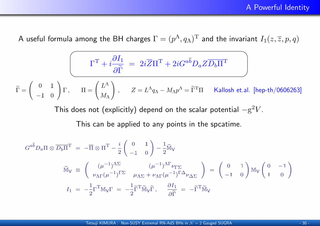
A useful formula among the BH charges Γ = (pΛ, qΛ)T and the invariant I1(z, z, p, q)�
�
�
�ΓT + i
∂I1
∂Γ= 2iZΠT + 2iGabDaZDbΠT
Γ =
(0 1
−1 0
)Γ , Π =
(LΛ
MΛ
), Z = LΛqΛ −MΛp
Λ = ΓTΠ Kallosh et.al. [hep-th/0606263]
This does not (explicitly) depend on the scalar potential −g2V .
This can be applied to any points in the spcatime.
Gab
DaΠ ⊗ DbΠT
= −Π ⊗ ΠT −
i
2
0 1
−1 0
!
−1
2eMV
eMV ≡
(µ−1)ΛΣ (µ−1)ΛΓνΓΣ
νΛΓ(µ−1)ΓΣ µΛΣ + νΛΓ(µ−1)Γ∆ν∆Σ
!
=
0 1
−1 0
!
MV
0 −1
1 0
!
I1 = −1
2Γ
TMVΓ = −1
2eΓ
TeMVeΓ ,
∂I1
∂eΓ= −eΓT
eMV
Tetsuji KIMURA : Non-SUSY Extremal RN-AdS BHs in N = 2 Gauged SUGRA - 30 -

Single Modulus Model: T3-model
Single modulus model (a = 1): F =(X1)3
X0
Z = eK/2(q0 + q t− 3p t2 + p0 t3
), t =
X1
X0
eK =i
(t− t)3, Gtt = − 3
(t− t)2≡ et
b1 etb1 δb1b1, Cttt =
6i(t− t)3
Search the sol. w/ V = −3|Z|2 + |Db1Z|2 < 0 → Z 6= 0
Consider non-SUSY sol. → Db1Z 6= 0
⇓
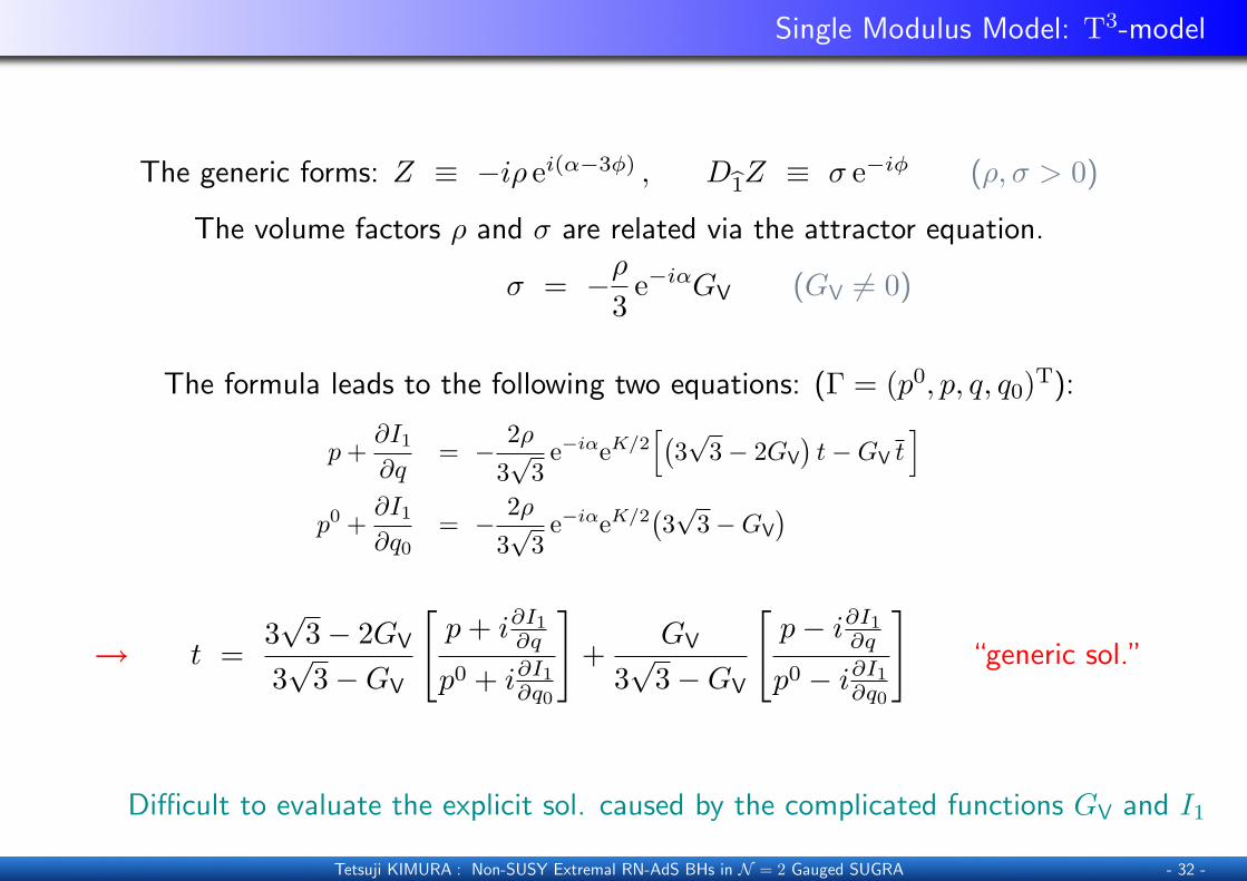
The generic forms of the central charge and its derivative:
Z ≡ −iρ ei(α−3φ) , Db1Z ≡ σ e−iφ (ρ, σ > 0)
[hep-th/0606263]
Tetsuji KIMURA : Non-SUSY Extremal RN-AdS BHs in N = 2 Gauged SUGRA - 31 -
Single Modulus Model: T3-model
The generic forms: Z ≡ −iρ ei(α−3φ) , Db1Z ≡ σ e−iφ (ρ, σ > 0)
The volume factors ρ and σ are related via the attractor equation.
σ = −ρ3
e−iαGV (GV 6= 0)
The formula leads to the following two equations: (Γ = (p0, p, q, q0)T):
p+∂I1∂q
= − 2ρ3√
3e−iαeK/2
[(3√
3− 2GV
)t−GV t
]p0 +
∂I1∂q0
= − 2ρ3√
3e−iαeK/2
(3√
3−GV
)
→ t =3√
3− 2GV
3√
3−GV
[p+ i∂I1
∂q
p0 + i∂I1∂q0
]+
GV
3√
3−GV
[p− i∂I1
∂q
p0 − i∂I1∂q0
]“generic sol.”
Difficult to evaluate the explicit sol. caused by the complicated functions GV and I1
Tetsuji KIMURA : Non-SUSY Extremal RN-AdS BHs in N = 2 Gauged SUGRA - 32 -
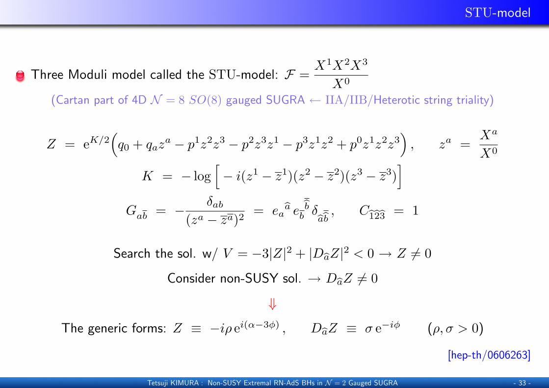
STU-model
Three Moduli model called the STU-model: F =X1X2X3
X0
(Cartan part of 4D N = 8 SO(8) gauged SUGRA ← IIA/IIB/Heterotic string triality)
Z = eK/2(q0 + qaz
a − p1z2z3 − p2z3z1 − p3z1z2 + p0z1z2z3), za =
Xa
X0
K = − log[− i(z1 − z1)(z2 − z2)(z3 − z3)
]Gab = − δab
(za − za)2= ea
ba eb
bb δbabb, C
b1b2b3 = 1
Search the sol. w/ V = −3|Z|2 + |DbaZ|2 < 0 → Z 6= 0
Consider non-SUSY sol. → DbaZ 6= 0
⇓
The generic forms: Z ≡ −iρ ei(α−3φ) , DbaZ ≡ σ e−iφ (ρ, σ > 0)
[hep-th/0606263]
Tetsuji KIMURA : Non-SUSY Extremal RN-AdS BHs in N = 2 Gauged SUGRA - 33 -

STU-model
The generic forms: Z ≡ −iρ ei(α−3φ) , DbaZ ≡ σ e−iφ (ρ, σ > 0)
The volume factors ρ and σ are related via the attractor equation.
σ = −ρ e−iαGV (GV 6= 0)
The formula leads to the following two equations:
pa +∂I1∂qa
= −2ρ e−iαeK/2[(
1−GV
)za − 2GV z
a]
p0 +∂I1∂q0
= −2ρ e−iαeK/2(1− 3GV
)
→ za = V 2eff
[pa + i∂I1
∂qa
p0 + i∂I1∂q0
]+ (1− V 2
eff)
[pa − i∂I1
∂qa
p0 − i∂I1∂q0
]“generic sol.”
Neither Veff = 1 nor Veff = 0
Difficult to evaluate the explicit sol. caused by the complicated functions GV and I1
Tetsuji KIMURA : Non-SUSY Extremal RN-AdS BHs in N = 2 Gauged SUGRA - 34 -

Another Example in T3-model
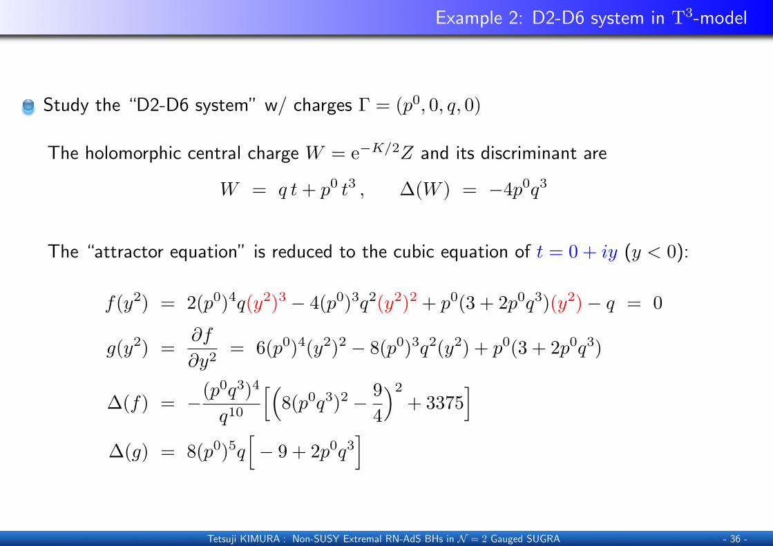
Example 2: D2-D6 system in T3-model
Study the “D2-D6 system” w/ charges Γ = (p0, 0, q, 0)
The holomorphic central charge W = e−K/2Z and its discriminant are
W = q t+ p0 t3 , ∆(W ) = −4p0q3
The “attractor equation” is reduced to the cubic equation of t = 0 + iy (y < 0):
f(y2) = 2(p0)4q(y2)3 − 4(p0)3q2(y2)2 + p0(3 + 2p0q3)(y2)− q = 0
g(y2) =∂f
∂y2= 6(p0)4(y2)2 − 8(p0)3q2(y2) + p0(3 + 2p0q3)
∆(f) = −(p0q3)4
q10
[(8(p0q3)2 − 9
4
)2
+ 3375]
∆(g) = 8(p0)5q[− 9 + 2p0q3
]
Tetsuji KIMURA : Non-SUSY Extremal RN-AdS BHs in N = 2 Gauged SUGRA - 36 -

Example 2: D2-D6 system in T3-model
The various values at the attractor point are
Z∣∣∣horizon
= −i(q − p0y2)√− 1
8y6= 0 , DtZ
∣∣∣horizon
= −(q + 3p0 y2)√− 1
32y36= 0
I1 =q2 + 3(p0)2y4
−6y> 0
Λ =2q2y
3((p0)2y2 − q
)2< 0
SBH =−3 +
√9 + 4q2
(q − (p0)2y2
)2(q2 + 3(p0)2y4
)−4q2(q − (p0)2y2)2y
> 0
The solution of the Modulus t = 0 + iy (y < 0) is given as
y2 = A+B or A+ ω±B , ω3 = 1
A =2q3p0
, B =1
6(p0)3q
(C1/3 +
14(p0)2
∆(g)C1/3
)C = −54(p0)5q3 − 8(p0)6q6 + 3
√3p0√−q2∆(f) , with p0q3 > 0
Tetsuji KIMURA : Non-SUSY Extremal RN-AdS BHs in N = 2 Gauged SUGRA - 37 -

Example 2’: D2-D6 system in T3-model
Compare our result to the (non-)SUSY solution of the RN-BH w/ Λ = 0
non-BPS solution:
t = 0 + iy , y = −√
q
3p0
Z∣∣∣horizon
=iq
3√
2
( 3p0
q
)1/4
6= 0 , DtZ∣∣∣horizon
= − q
2√
2
( 3p0
q
)3/4
6= 0
SBH = I1 = |Z|2 +GttDtZDtZ = 4|Z|2 =23
√p0q3
3> 0 , Λ = 0
1/2-BPS solution:
t = 0 + iy , y = −√− q
3p0
Z∣∣∣horizon
=−i√
2q3
(− 3p0
q
)1/4
6= 0 , DtZ∣∣∣horizon
= 0
SBH = I1 = |Z|2 =23
√−p
0q3
3> 0 , Λ = 0
Tetsuji KIMURA : Non-SUSY Extremal RN-AdS BHs in N = 2 Gauged SUGRA - 38 -

Hypermultiplets

Moduli Space of Hypermultiplets
Action including hypermultiplets:
S =∫
d4x√−g{ 1
2κ2R−Gab(z, z)∂µz
a∂µzb−huv(q)∇µqu∇µqv
+14µΛΣ(z, z)FΛ
µνFΣµν +
14νΛΣ(z, z)FΛ
µν(∗FΣ)µν
− g2V (z, z, q)
+ (fermionic terms)}
Moduli space of hypermultiplets = quaternionic geometry
We borrow the description in (non)geometric flux compactifications scenarios
arXiv:0911.2708 etc.
{qu}4nH + 4
= {zi, z}2nH(SKG)
+ {ξi, ξi}2nH
+ {ϕ, a, ξ0, ξ0}4 (universal)
(special quaternionic geometry)
Tetsuji KIMURA : Non-SUSY Extremal RN-AdS BHs in N = 2 Gauged SUGRA - 40 -

Moduli Space of Hypermultiplets
Contribution of hypermultiplets to the kinematics and potential:
huv dqudqv = Gi dzi dz +SKGH
(dϕ)24D dilaton
+14e4ϕ(
daaxion− ξT CH dξ
)2− 12e2ϕdξT MH dξ
scalars from RR
∇µqu = ∂µq
u + g kuΛA
Λµ , kΛ = −
[2qΛ + eΛ
I(CHξ)I] ∂∂a− eΛI ∂
∂ξI
P+ ≡ P1 + iP2 = 2eϕ ΠTV QCH ΠH
P− ≡ P1 − iP2 = 2eϕ ΠTV QCH ΠH
P3 = e2ϕ ΠTV CV(c+ Qξ)
MV,H =
(µ+ νµ−1ν −νµ−1
−µ−1ν µ−1
)V,H
µV,H = ImNV,H , νV,H = ReNV,H
,QΛ
I =
(eΛ
I eΛI
mΛI mΛI
), CV,H =
(0 1
−1 0
)QΛ
I = CTV QCH
ΠH = eKH/2(ZI,GI)T, zi = Zi/Z0: SKG variables in hypermoduli
ΠV = eKV/2(XΛ,FΛ)T: SKG variables in vector modulic = (pΛ, qΛ)T can also be regarded as the BH charges
Tetsuji KIMURA : Non-SUSY Extremal RN-AdS BHs in N = 2 Gauged SUGRA - 41 -

Hypermultiplets
huv∇µqu∇µqv = (∂µϕ)2 +
14e4ϕ(∇µa− ξ0∇µξ0 + ξ0∇µξ
0)2
∇µa = ∂µa− g(2qΛ + eΛ0ξ0 − eΛ0ξ
0)AΛµ
∇µξ0 = ∂µξ
0 − g(eΛ0)AΛµ , ∇µξ0 = ∂µξ0 − g(eΛ0)AΛ
µ
V (z, z, q) = GabDaP3DbP3 − 3|P3|2 , P3 = e2ϕ(Z + Zξ
)Z ≡ LΛqΛ −MΛp
Λ , Zξ ≡ LΛ(eΛ0ξ0 − eΛ0ξ0)−MΛ(mΛ
0ξ0 −mΛ0ξ0)
Very complicated even when we focus only on the Universal hypermultiplet
compared to the system only with Vector multiplets
arXiv:1005.3650� �SUSY BH-sol. in stationary, axisymmetric, asymptotically flat spacetime
has constant universal hypermoduli
and vector multiplets which follow the ordinary attractor mechanism� �How is non-SUSY RN(-AdS) BH-sol. in the presence of Universal hypermoduli?
−→ work in progress
Tetsuji KIMURA : Non-SUSY Extremal RN-AdS BHs in N = 2 Gauged SUGRA - 42 -
Related Documents


