Non-scanning Fluorescence Confocal Microscopy using Laser Speckle Illumination by Shihong Jiang, BEng. School of Electrical and Electronic Engineering Thesis submitted to The University of Nottingham for the Degree of Doctor of Philosophy October 2005

Welcome message from author
This document is posted to help you gain knowledge. Please leave a comment to let me know what you think about it! Share it to your friends and learn new things together.
Transcript

Non-scanning Fluorescence Confocal Microscopy
using Laser Speckle Illumination
by
Shihong Jiang, BEng.
School of Electrical and Electronic Engineering
Thesis submitted to The University of Nottingham
for the Degree of Doctor of Philosophy
October 2005

Abstract
Confocal scanning microscopy (CSM) is a much used and advantageous form of
microscopy. Although CSM is superior to conventional microscopy in many
respects, a major disadvantage is the complexity of the scanning process and the
sometimes long time to perform the scan. In this thesis a novel non-scanning
fluorescence confocal microscopy is investigated. The method uses a random time-
varying speckle pattern to illuminate the specimen, recording a large number of
independent full-field frames without the need for a scanning system. The recorded
frames are then processed in a suitable way to give a confocal image. The goal of this
research project is to confirm the effectiveness and practicality of speckle-
illumination microscopy and to develop this proposal into a functioning microscope
system. The issues to be addressed include modelling of the system performance,
setting up experiments, computer control and image processing. This work makes the
following contributions to knowledge:
• The development of criteria for system performance evaluation
• The development of methods for speckle processing, whereby the number of
frames required for an image of acceptable quality can be reduced
• The implementation of non-scanning fluorescence confocal microscopy based
upon separate recording of the speckle patterns and the fluorescence frames,
demonstrating the practicality and effectiveness of this method
• The realisation of real-time image processing by optically addressed spatial
light modulator, showing how this new form of optical arrangement may be
used in practice
The thesis is organised into three main segments. Chapters 1-2 review related work
and introduce the concepts of fluorescence confocal microscopy. Chapters 3-5
i

discuss system modelling and present results of performance evaluation. Chapters 6-
8 present experimental results based upon the separate recording scheme and the
spatial light modulation scheme, draw conclusions and offer some speculative
suggestions for future research.
ii

Acknowledgements
The author would like to thank Dr John Walker for his original and creative work in
the field of fluorescence confocal microscopy which provides a well-defined
research project for a PhD student, especially for his effort in providing the author
with the opportunity to carry out this work under his direct supervision. Without
John Walker’s expert knowledge of confocal microscopy and of relevant disciplines,
the completion of this work would have been an extremely difficult undertaking. The
author would also like to thank Professor Mike Somekh, Dr Barrie Hayes-Gill, Dr C.
W. See and other staff within the Applied Optics Group for their kind support and
helpful advice throughout his PhD studies. Special thanks are due to the International
Office of the University of Nottingham for providing funding to make the three-year
research possible. Thanks also go to the many members of staff and postgraduate
students who assisted the author with technical data, thoughtful comments as well as
equipment and lab tools for building the experimental systems.
Other people to whom the author is indebted for being very valuable to him
with his life and work are his wife Hong Ye, his son Weifeng and his mother Airu
Sun.
iii

Table of Contents
1. Introduction .............................................................................................................1
1.1 Laser confocal scanning microscopy ....................................................................2
1.2 Tandem scanning confocal microscopy................................................................3
1.3 Structured-light illumination.................................................................................5
1.3.1 Axially structured illumination .................................................................6
1.3.2 Laterally structured illumination...............................................................7
1.4 Laser speckle illumination ....................................................................................9
1.5 Remarks ..............................................................................................................10
2. Image formation ....................................................................................................13
2.1 Scanning fluorescence confocal microscopy ......................................................13
2.1.1 Low-aperture case ...................................................................................14
2.1.2 High-aperture case ..................................................................................15
2.2 Depth discrimination property ............................................................................18
2.3 Lateral resolution ................................................................................................19
2.4 Non-scanning fluorescence confocal microscopy using speckle illumination ...22
3. Simulation..............................................................................................................26
3.1 Fourier optics approach.......................................................................................26
3.2 Shot noise ............................................................................................................29
3.3 Additive white noise ...........................................................................................31
3.4 Quantisation ........................................................................................................34
3.5 Results .................................................................................................................35
3.5.1 Laser speckle...........................................................................................35
3.5.2 Uniform fluorescent planar object ..........................................................36
3.5.3 Point object .............................................................................................39
iv

4. Performance evaluation .........................................................................................45
4.1 Intensity non-uniformity .....................................................................................45
4.2 Nonlinear variation of image intensity................................................................46
4.3 Depth discrimination property ............................................................................49
4.4 Lateral resolution ................................................................................................50
5. Speckle processing ................................................................................................52
5.1 A-Law compression ............................................................................................53
5.2 Binary speckle.....................................................................................................61
5.3 Analysis...............................................................................................................64
6. Experimental confirmation ....................................................................................68
6.1 Experimental arrangement ..................................................................................68
6.2 Apparatus ............................................................................................................69
6.2.1 Laser........................................................................................................69
6.2.2 CCD camera ............................................................................................71
6.2.3 Specimen.................................................................................................72
6.2.4 Filters ......................................................................................................73
6.2.5 Rotating diffuser .....................................................................................73
6.3 Principal parameters............................................................................................74
6.4 Light budget ........................................................................................................76
6.5 Image noise analysis ...........................................................................................76
6.6 Experimental results............................................................................................78
6.6.1 Acquisition of raw images ......................................................................78
6.6.2 Postprocessed images and discussion .....................................................80
7. Real-time optical data processing..........................................................................88
7.1 Experimental arrangement ..................................................................................89
v

7.2 The transmissive miniature liquid crystal display...............................................91
7.3 Principal parameters............................................................................................92
7.4 Optical data processing .......................................................................................93
7.5 Experimental results with digital frame averaging ...........................................105
7.6 Image manipulation...........................................................................................111
7.7 Experimental results with averaging by CCD charge accumulation ................122
8. Conclusion and further work ...............................................................................127
8.1 Conclusion ........................................................................................................128
8.2 Further work......................................................................................................131
Bibliography..................................................................................................................133
vi
Chapter 1. Introduction
1. Introduction
“Real knowledge is to know the content of one’s ignorance.”
Confucius, 551 BC - 479
Confocal scanning microscopy (CSM), invented by Minsky in 1955 [1], is a widely
used technique in many fields of science particularly in the life and biosciences [2-4].
Unlike conventional microscopy, CSM illuminates and images only one small spot at
a time, in the focal plane of the objective. The sequences of points of light from the
specimen are detected through a pinhole and the output from the detector is built into
an image and displayed by a computer. CSM has many advantages over conventional
microscopy, including a valuable depth discrimination property that permits three-
dimensional image reconstruction, the improved lateral resolution and a reduced
effect of flare or scattered light contributing to the image. As CSM is a powerful and
irreplaceable tool for studying biological cells in vivo or in vitro, its capabilities have
been extended to include fluorescence detection and lifetime imaging [5-8], and to
improve its spatial resolution [9-12]. Progress in multiphoton excitation processes,
interest in the burgeoning field of single-molecule biophysics have recently pushed
CSM to its ultimate level of sensitivity [13-15].
Because a confocal image is built up pixel by pixel by scanning the
illuminated spot over the specimen, it is intrinsically time-consuming if a large area
needs to be searched. The noise level of confocal images can be easily higher than
wide-field images [16], particularly at high scan speeds, due to the limited number of
photons of fluorescence that can be collected from a diffraction-limited area in pixel
dwell times lasting fractions of a microsecond [17, 18]. Moreover, the light gathering
ability of CSM is low due to the use of a pinhole. During the last few decades,
1

Chapter 1. Introduction
various efforts have been undertaken to circumvent these limitations but retain the
advantages of confocal microscopy. Major advances include direct view, or tandem
scanning confocal microscopy, structured-light illumination such as standing wave
illumination, grid pattern illumination and laser speckle illumination. In this chapter
a general description and review of several state-of-the-art confocal microscopic
techniques is given.
1.1 Laser confocal scanning microscopy
Lasers are the most common light source for confocal scanning microscopes as they
provide ideal types of excitation light for fluorescence microscopy applications. In
Laser Scanning Confocal Microscope (LSCM) shown in Fig. 1.1 a laser beam is
focused by an objective onto a fluorescent specimen through an X-Y deflection
mechanism. The mixture of reflected light and emitted fluorescent light is captured
by the same objective and (after conversion into a static beam by the X-Y scanner
device) is focused onto a photomultiplier via a dichroic beamsplitter. Commonly, a
raster scan is generated by reflection from two moving mirrors, aligned at 90° with
the motion of each mirror being driven by a linear saw-tooth control signal. This
scanning unit is elaborately designed so that the laser location is changing linearly
without image distortion. Current LSCMs collect images with a scan speed of up to 5
frames/second with 512×512 pixels, such as the ZEISS LSM 510 META in which
the scanner consists of two independent galvanometric scanning mirrors. By varying
the distance between the objective and the specimen, users can generate a Z-series
that dissect through the specimen with a Z-scan interval down to 50 –100 nm. Object
features in the order of 0.2 µm can be resolved, and height differences of less than
0.1 µm are made visible [19].
2

Chapter 1. Introduction
Fig. 1.1. A typical LSCM system
(From http://yakko.bme.virginia.edu/phy506/system.gif)
1.2 Tandem scanning confocal microscopy
Mojmir Petran [20] pioneered the use of Nipkow disks in CSM, where the specimen
is illuminated with a large number of scanning beams in tandem to improve scanning
speed. A Nipkow disk is an opaque circular disk perforated with small holes
arranged at equal angular separations arranged in an Archimedean spiral. The holes
trace a raster scanning pattern when the disk is spun around its centre. In the tandem
scanning confocal microscope, the Nipkow disk can be spun rapidly enough to
provide video-rate (30 frames/second) imaging and was used in early experiments on
television and later in Petran’s confocal microscope. A typical Nipkow-disk confocal
microscope arrangement is shown in Fig. 1.2. The downside of the Nipkow-disk type
system is that the efficiency of light transmission is low, usually less than 5%, often
3
Chapter 1. Introduction
resulting in fluorescence that is too dim to take advantage of the high imaging speed
of the system [21].
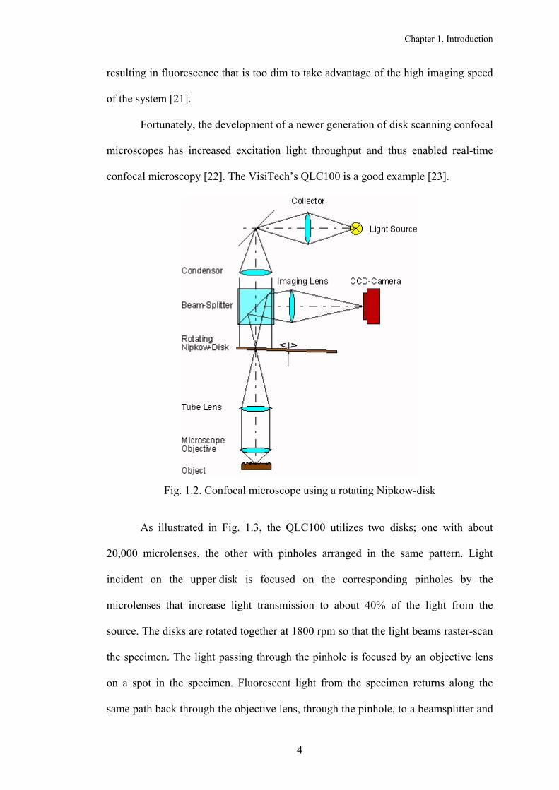
Fortunately, the development of a newer generation of disk scanning confocal
microscopes has increased excitation light throughput and thus enabled real-time
confocal microscopy [22]. The VisiTech’s QLC100 is a good example [23].
Fig. 1.2. Confocal microscope using a rotating Nipkow-disk
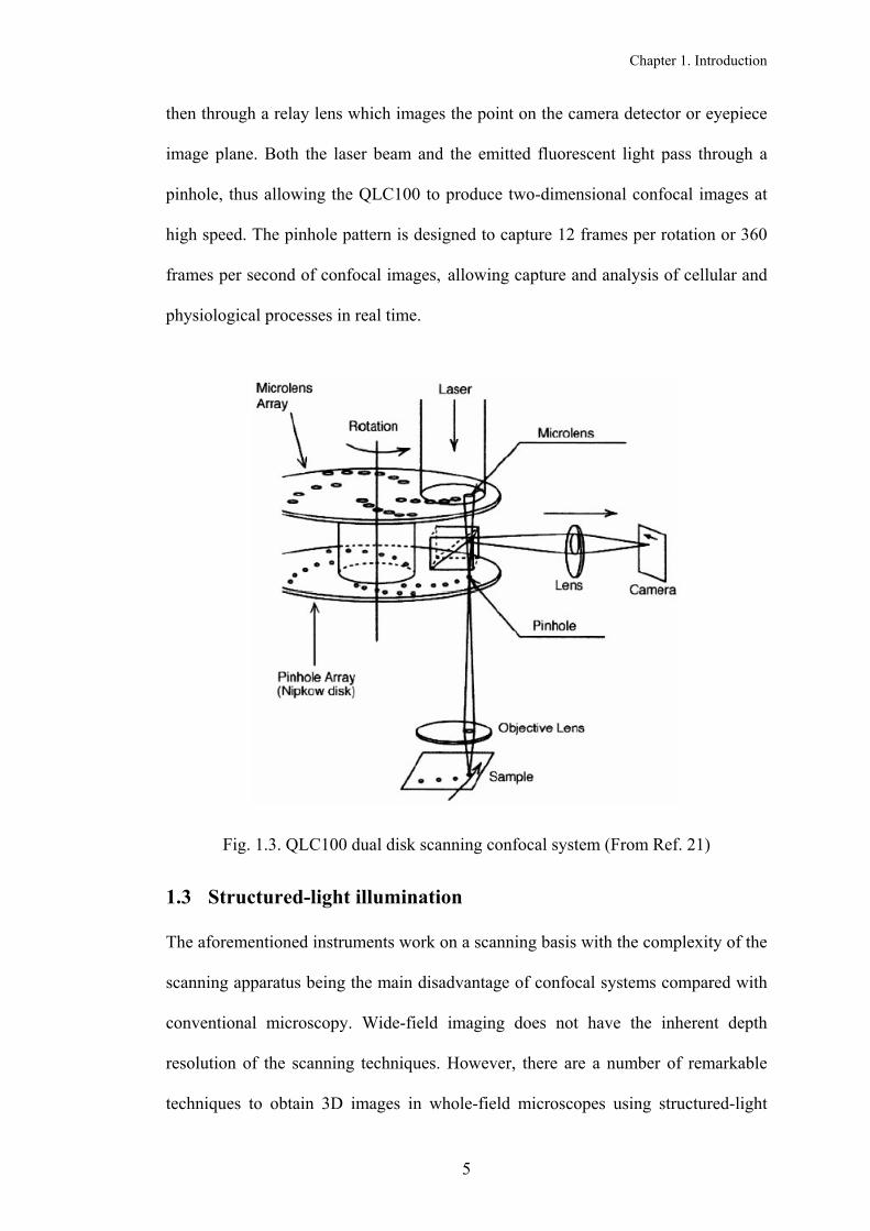
As illustrated in Fig. 1.3, the QLC100 utilizes two disks; one with about
20,000 microlenses, the other with pinholes arranged in the same pattern. Light
incident on the upper disk is focused on the corresponding pinholes by the
microlenses that increase light transmission to about 40% of the light from the
source. The disks are rotated together at 1800 rpm so that the light beams raster-scan
the specimen. The light passing through the pinhole is focused by an objective lens
on a spot in the specimen. Fluorescent light from the specimen returns along the
same path back through the objective lens, through the pinhole, to a beamsplitter and
4
Chapter 1. Introduction
then through a relay lens which images the point on the camera detector or eyepiece
image plane. Both the laser beam and the emitted fluorescent light pass through a
pinhole, thus allowing the QLC100 to produce two-dimensional confocal images at
high speed. The pinhole pattern is designed to capture 12 frames per rotation or 360
frames per second of confocal images, allowing capture and analysis of cellular and
physiological processes in real time.
Fig. 1.3. QLC100 dual disk scanning confocal system (From Ref. 21)
1.3 Structured-light illumination
The aforementioned instruments work on a scanning basis with the complexity of the
scanning apparatus being the main disadvantage of confocal systems compared with
conventional microscopy. Wide-field imaging does not have the inherent depth
resolution of the scanning techniques. However, there are a number of remarkable
techniques to obtain 3D images in whole-field microscopes using structured-light
5

Chapter 1. Introduction
illumination. Here two important structured illumination techniques will be
discussed. Other methods include image interference microscopy (InM) invented by
Mats GL Gustafsson [24, 25] and harmonic excitation light microscopy (HELM) by
Jan T. Frohn et al [26-28]. These methods are focused on obtaining optical
superresolution, so they are beyond the scope of this thesis and will not be discussed
here.
1.3.1 Axially structured illumination
Standing-wave fluorescence microscopy (SWFM) was invented by Brent Bailey et
al. in 1993 [29-32]. Its principle is shown in Fig. 1.4 where two collimated beams
from a laser are directed at the specimen from opposite sides. The coherent, equal-
amplitude beams (arrows) cross symmetrically relative to the microscope axis, and
are s-polarised. The interference of the beams then produces planar nodes and
antinodes (alternating dashed and solid lines) oriented perpendicular to the
microscope axis. Fluorescence is therefore excited in the specimen in a series of
equally spaced laminar zones, and nulled at the nodes. By optically shifting the
standing-wave field planes up or down within the specimen, it is possible to excite or
null structures selectively at different levels within the depth-of-field of the
microscope.
θlens 1
specimen
lens 2
Fig. 1.4. Schematic of axial standing wave illumination (From Ref. 30)
6

Chapter 1. Introduction
The intensity of the standing-wave field is constant over any plane parallel to
the x,y-plane, and varies sinusoidally with the axial (z) coordinate as:
)cos(1]))(cos/4cos[(1 0 φφθλπ ++=++= KzznIex (1.1)
where n is the specimen refractive index, λ is the laser wavelength, and φ is the
relative phase of the two beams which can be adjusted with very high precision by
moving a mirror with a piezo-electric drive. The image equation with the camera
held fixed in the image focal plane and the object stepped through focus, is:
(1.2) ∫∫∫ ++∆−=∆ zyxzyxyxSKzzzyxOzyxI ddd),,;','()]cos(1)[,,(),','( φ
where S is the microscope’s intensity point spread function and ∆ is the focus
position of the object. Since the value of φ is unknown, at least three images,
corresponding to a phase shift of φ between them, need to be acquired at each focal
plane to determine the optically sectioned image I. The axial resolution can be better
than a quarter of the node spacing, or 0.045 µm, under typical conditions.
z
Because the axial response to a point object in the SWFM has a ringing
effect, the sample thickness is limited by the period of the standing wave field unless
there is a priori knowledge. A further development of this method, called excitation
field synthesis, improves the sectioning capability by utilizing a superposition of
different interference patterns giving one sharp interference maximum.
1.3.2 Laterally structured illumination
A simple method of using grid pattern illumination was proposed in 1997 by which
optically sectioned fluorescence images may be obtained with conventional
microscopes [33-35].
As illustrated in Fig.1.5, a one-dimensional grid pattern is projected onto
the specimen. A CCD camera captures three images, I1, I2 and I3, corresponding to a
7

Chapter 1. Introduction
relative spatial phase shift of the grid of 120° between them. These images are then
processed by
2/12
322
312
21 })()(){(32 IIIIIII p −+−+−=
(1.3)
lamp
specimen
grid
sync
piezo
CCD camera
Fig. 1.5. Schematic of the optical arrangement using grid pattern illumination
(From Ref. 33)
The processed image Ip exhibits optical sectioning in the same fashion as a confocal
microscope, provided a suitable spatial frequency of the grid is chosen. This is
because in a conventional microscope only the zero spatial frequency within the
transfer function does not attenuate with defocus, one will thus obtain an optically
sectioned image of the object with the grid pattern superimposed. The rate of
attenuation with defocus will depend on the particular spatial frequency of the grid
that is projected onto the object. The fundamental issue to be addressed is how to
remove the unwanted grid pattern from the optically sectioned image. If v denotes
8
Chapter 1. Introduction
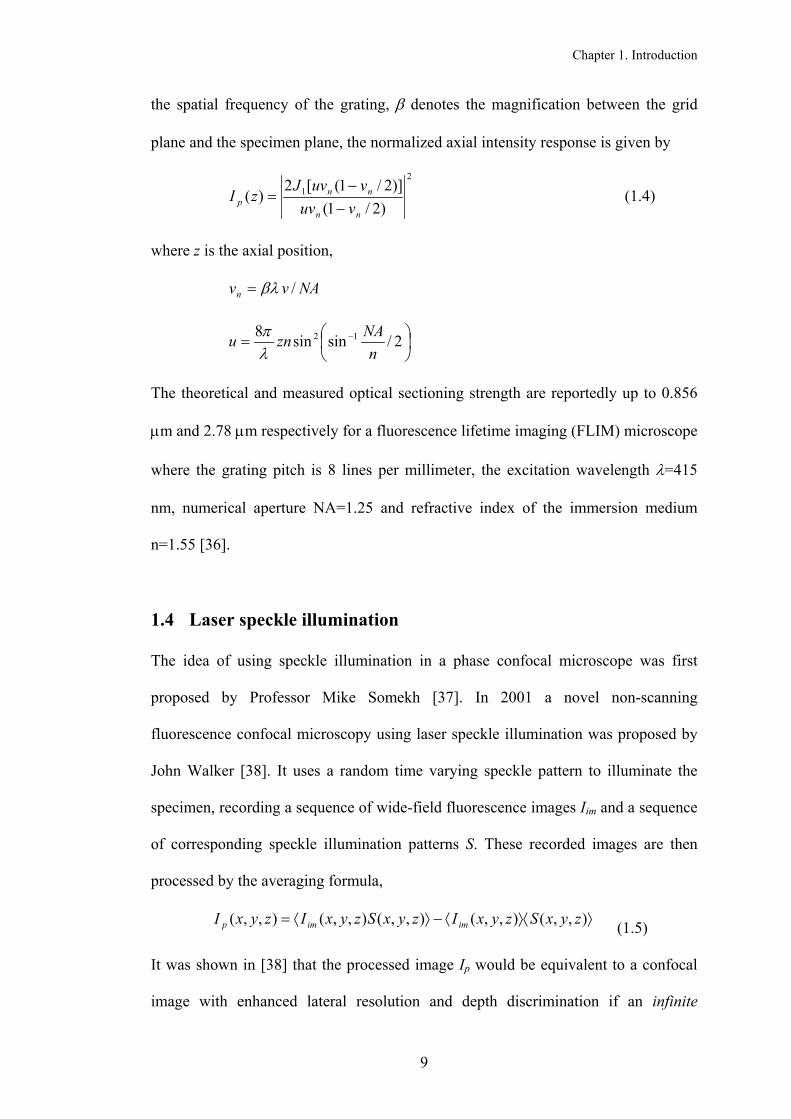
the spatial frequency of the grating, β denotes the magnification between the grid
plane and the specimen plane, the normalized axial intensity response is given by
2
1
)2/1()]2/1([2
)(nn
nnp vuv
vuvJzI
−−
= (1.4)
where z is the axial position,
NAvvn /βλ=
= − 2/sinsin8 12
nNAznu
λπ
The theoretical and measured optical sectioning strength are reportedly up to 0.856
µm and 2.78 µm respectively for a fluorescence lifetime imaging (FLIM) microscope
where the grating pitch is 8 lines per millimeter, the excitation wavelength λ=415
nm, numerical aperture NA=1.25 and refractive index of the immersion medium
n=1.55 [36].
1.4 Laser speckle illumination
The idea of using speckle illumination in a phase confocal microscope was first
proposed by Professor Mike Somekh [37]. In 2001 a novel non-scanning
fluorescence confocal microscopy using laser speckle illumination was proposed by
John Walker [38]. It uses a random time varying speckle pattern to illuminate the
specimen, recording a sequence of wide-field fluorescence images Iim and a sequence
of corresponding speckle illumination patterns S. These recorded images are then
processed by the averaging formula,
⟩⟩⟨⟨−⟩⟨= ),,(),,(),,(),,(),,( zyxSzyxIzyxSzyxIzyxI imimp (1.5)
It was shown in [38] that the processed image Ip would be equivalent to a confocal
image with enhanced lateral resolution and depth discrimination if an infinite
9

Chapter 1. Introduction
ensemble of frames were used. The theory of this method will be given in section
2.4. Here the physical significance of Eq. (1.5) is provided as the following:
The dynamic speckles falling on the specimen can be thought of as acting like
the illumination spots in a tandem scanning confocal microscope. The multiplication
of each fluorescent frame Iim by the same illumination speckle pattern S mimics the
returning fluorescent light from the specimen passed through the individual pinholes
in a Nipkow disk. The difference is that the speckles are random in both position and
in intensity, hence an average over a large number of speckle patterns must be
obtained. Depth discrimination occurs because parts of the sample away from the
focal plane are illuminated by the speckles formed in that plane. Since these speckles
are different, due to the fact that the speckle pattern associated with the sample is
three-dimensional in space, Iim is no longer correlated with S, and the ensemble of
their product (the first term) tends to the multiplication of their ensembles (the
second term), leaving a null image Ip.
This method avoids the scanning system and pinhole required in a
conventional CSM but retains the advantages of confocal microscopy. Experiments
to confirm the practicality and effectiveness of this method were made recently [39,
40]. Detailed discussions of this method will be given in the following chapters.
1.5 Remarks
An important feature of laser confocal scanning microscopes is the capability of
depth discrimination. This depth response derives from the use of a point detector
and is especially useful in the tomographic observation of thick fluorescent
specimens. In many applications, however it is not possible to use as small a detector
as we would like because of signal to noise problems. This is particularly true in
10

Chapter 1. Introduction
fluorescent imaging because the signal level is weak. The optical sectioning becomes
progressively worse as the pinhole size becomes larger (see Page 114 of Ref. 46). On
the other hand, the signal to noise ratio of the image increases as the pinhole size
increases, reaches a maximum value for an optimum pinhole size, and then decreases
as the pinhole is made larger.
Tandem scanning is an elegant solution to the scan-time problem. The first
version of this design suffered from the poor transmission of illumination through the
disc. However, this problem has been alleviated by a recent design that uses
microlenses to focus 40% of the illuminating light through the pinholes. This system,
has found wide utility among cell biologists. Because the size of pinholes is fixed,
resolution is necessarily worse when using lower power objectives compared with
the LSCM system where the pinhole size is adjustable [41].
Structured-light and laser speckle illumination techniques require no scanning
and have the potential to rapidly acquire data with a high signal-to-noise ratio.
Standing wave fluorescence microscopy (SWFM) is a wide-field technique which
provides high axial resolution in thin, fluorescently labelled specimens. However,
this method does not extend the lateral resolution. A weakness of SWFM is that its
optical transfer function contains large gaps between the central band and the
sidebands, the so-called “information gap” [42].
Grid pattern illumination does permit optically sectioned images to be
obtained but no information on the improved lateral resolution has been reported.
Furthermore, practical applications of structured illumination microscopy often
suffer from artefacts that can be observed as residual stripe patterns due to the
inaccurate grating shifts, non-sinusoidal grating patterns or fluctuation of excitation
light during acquisition [43].
11

Chapter 1. Introduction
Speckle illumination system makes it possible to perform wide-field
fluorescence confocal imaging with minimal modification to a conventional
microscope without the signal-to-noise problem associated with the pinhole size in a
scanning system. An advantage of wide-field microscopy is that the CCD camera has
a quantum efficiency (QE) between 20% and 80% depending on the wavelength.
However the QE of the photomultiplier used in CSMs is only 10% or less, although
it has very low detector noise levels. So to obtain the same signal level, typically 400
photons per pixel as for the CCD camera, the photomultiplier would require 4000
photons in a single scan. This is usually not possible for a fluorescence CSM.
Laser speckle illumination seems superior to other illumination techniques in
the sense that it provides a fully confocal imaging response. However this is at the
price of recording a huge number of frames, so that the recording time could be very
long. The attractiveness with this method would rely on the frame rate of the
recording device (CCD). Since current CCD technology allows a frame rate of 291
frames/s at the resolution of 480×640 pixels to be reached (C7770, Hamamatsu
Photonics), imaging with speckle illumination on the second scale should be possible
if the image obtained by averaging over 500 frames has an acceptable visual quality.
With the advent of spatial light modulator technology, it is possible to multiply two
frames optically in real time and average frames by taking a single CCD readout. An
advantage of the CCD camera is that “it can integrate the signal in analogue form on
the chip during a prolonged exposure, which avoids problems with digitisation errors
and readout noise encountered when accumulating an image by averaging successive
noisy individual frames in digital memory [44]”, thus increasing the attractiveness of
this method.
12
Chapter 2. Image formation
2. Image formation
"Everything should be made as simple as possible, but not simpler."
Albert Einstein, 1879 - 1955 There is an extensive literature [45-47] on the theory of image formation in confocal
microscopes, based on either the scalar or the vector far-field diffraction imaging
theory depending on whether a low-aperture or a high-aperture system is considered.
In this chapter calculations are made for both the cases by using the existing theory
to obtain the point spread function (response to a point source) in a fluorescence
confocal system. It should be noted that the size of the pinhole in a scanning system
is assumed to be ideally small, although this will cause signal-to-noise problems in
fluorescence imaging, and the optical systems involved are assumed aberration-free.
2.1 Scanning fluorescence confocal microscopy
As illustrated in Fig. 2.1, if we denote by O the spatial distribution of the
fluorescence generation, we can write the intensity just behind the object as
proportional to | , where h is the amplitude point response of the first lens
imaging at a wavelength of
Oh 21 | 1
1λ . This intensity is then imaged at the fluorescence
wavelength, 2λ , by the second lens. For circular pupils the confocal image intensity
is given by
OvuhvuhI ⊗= 221 )/,/(),( ββ (2.1)
where is the amplitude point response of the second lens, 2h 12 / λλβ = (λ2> λ1 due
to the Stokes shift) is the ratio of the wavelengths. The optical units
13

Chapter 2. Image formation
α
λπ 2
1
sin2 zu =
αλπ sin2
1
rv = (2.2)
where z is the defocus distance of the object, r the radial coordinate, α the semi-angle
of aperture.
λ2 λ1
pinhole specimen
Fig. 2.1. Schematic of scanning fluorescence confocal microscopy
2.1.1 Low-aperture case
Assuming both lens have an identical small angular aperture, the scalar theory is then
applicable. Based on Fraunhofer’s approximation, the amplitude point response can
be written as
∫ −=1
0 02 d)()
21exp()(2),( ρρρρρ vJjuPvuh
(2.3)
where P is the pupil function defined as
>≤≤
=1,0
10,1)(
ρρ
ρP (2.4)
J0 is the Bessel function of the zeroth order. If the object consists of a point source,
then the image is given by
2|)/,/(),(|),( ββ vuhvuhvuI = (2.5)
Fig. 2.2 shows such an image in a system with m 5.01 µλ = , m 6.02 µλ = and the
numerical aperture taking different values. Note that Fig. 2.2(b) is just for
comparison with the vector solution to be discussed later. Compared with
14

Chapter 2. Image formation
conventional fluorescence microscopy, the central peak of the confocal response is
sharpened by a factor of 1.4 (measured at half-peak intensity).
(a) (b) 5.0=NA 1=NA
Fig. 2.2. Image of a single point source in a fluorescence confocal microscope
with scalar solution
2.1.2 High-aperture case
For high-aperture incoherent systems, the vector solution should be used [48, 49].
Consider an optical system of revolution, which images a point source at infinity on
the optical axis. The source is assumed to give rise to a linearly polarised
monochromatic wave, with the electric vector E in the x-direction. The vector can be
divided into a linear combination of a component within the meridional plane, E||,
plus a component perpendicular to it, E⊥, as illustrated in Fig. 2.3(a). After
undergoing refraction, the parallel part E|| is bent by θ, while the perpendicular part
E⊥ suffers no change. The bent vector Eθ’ at the exit pupil now exhibits also a part in
the direction of the z-axis, Ez, as shown in Fig. 2.3(b) [50]. The components of the
field vectors at a point P in the image region are given by
15

Chapter 2. Image formation
φ φ
y
E
E||
E⊥
’ Eθ’
x
(a) The lateral plane (b)
Fig. 2.3 A schematic diagram fo
)2cos( 20 φIIiAEx +−=
)2sin( 2 φIiAEy −=
)cos(2 1 φIAEz −=
where A is a constant, φ is the azimuth and
∫ +=
α
αθθθθ
000 sin
sin)cos1(sincos),( vJvuI
∫
=
α
αθθθ
01
21 si
cexpsinsinsincos),( jvJvuI
∫ −=
α
αθθθθ
022 sin
sin)cos1(sincos),( vJvuI
where J0, J1 and J2 are the Bessel functions of the
, Inn xxJ ≈)( 1 and I2 are of lower order than I0,
comparison with I0. Invoking
16
E||
of
Ez’
θ z
The meridional plane
r vector solution
(2.6.1)
(2.6.2)
(2.6.3)
θ
αθ
2 dsincosexp uj
(2.7.1)
θ
αθ
2 dnos u
(2.7.2)
θ
αθ
2 dsincosexp uj
(2.7.3)
first kind. For small semi-angle α,
so that they may be neglected in

Chapter 2. Image formation
θθ ≈sin
−
≈elsewhere1
2.7equation of phase in the2/1cos
2θθ
αθρ sin/=
equation (2.7.1) is then reduced to equation (2.3), the usual scalar solution, resulting
in the electric field in the image region being linearly polarised in the same direction
of the incoming wave. For large semi-angle, I1 and I2 cannot be neglected, the effect
of field components Ey and Ez becomes significant, thus causing the point spread
function to be asymmetric about the axis of the system.
The situation is quite different for fluorescence imaging. The fluorescent
radiation is completely incoherent and randomly polarised. The time-averaged
intensity distribution may be obtained by averaging the polarised fields over all
possible states of polarisation. After carrying out this averaging and by assuming that
the excitation light is circularly polarised [51], the intensity point response of the first
and second lens can be expressed as
22
21
2021 ),(),(2),(),(),(),( vuIvuIvuIvuwvuwvuw ++=== (2.8)
Note that the above expression is independent of φ, meaning that the point spread
function is circularly symmetric. The image of a point source in a high-aperture
fluorescence confocal microscope is then given by
)/,/(),(),( ββ vuwvuwvuI = (2.9)
Calculations are made for a system with m 5.01 µλ = , m 6.02 µλ = and the numerical
aperture taking different values. The results are shown in Fig. 2.4. It may be seen that
for the case of NA=0.5 the scalar solution is consistent with the vector one, but for
the case of NA=1 the scalar theory underestimates the correct diffraction limit. It is
natural to ask at what NA the scalar theory is no longer applicable. The consensus
17

Chapter 2. Image formation
(see, for example, Ref. [52]) is that the scalar approximation is good up to a NA
value of 0.5.
(a) (b) 5.0=NA 1=NA
Fig. 2.4. Image of a single point source in a fluorescence confocal microscope
with vector solution
2.2 Depth discrimination property
If we scan a uniform fluorescent planar object through focus, i.e., we set
)'( uuO −= δ , where δ is a delta function, u’ is a specified focal position, then the
power, or the integrated intensity, in the image, is given by
∫∞
=0
2int d)/,/(),()( vvvuhvuhuI ββ (2.10)
for the low-aperture case or by
∫∞
=0int d)/,/(),()( vvvuwvuwuI ββ (2.11)
for the high-aperture case. Note that the prime of u has been dropped. The depth
discrimination property can be evaluated in terms of the ratio of the out-of-focus
integrated intensity to the in-focus integrated intensity:
)0(/)( intint IuI (2.12)
18

Chapter 2. Image formation
The full-width at half-maximum (FWHM) for the curve thus obtained versus z-
direction is defined to be the axial resolution. Calculations are made using (2.10),
(2.11) and (2.12) for both the low-aperture and high-aperture systems. The results are
shown in Figs. 2.5 and 2.6 respectively. It may be observed that high-aperture
systems give better axial resolution.
2.3 Lateral resolution
By setting 0=u in (2.3), we get the image intensity distribution of a single point
source at the focal plane in a low-aperture system:
211
/)/()(4)(
⋅=
ββ
vvJ
vvJvI
(2.13)
The optimal resolution is achieved if 1=β . Fig. 2.7 and Fig. 2.8 show the image
intensity distribution of an in-focus single point source, obtained via scalar and
vector approaches respectively. As for the axial resolution, the FWHM for the
distribution versus radial direction is defined to be the lateral resolution.
19

Chapter 2. Image formation
Fig. 2.5. Depth discrimination property with the scalar solution ( m 5.01 µλ = ,
) 5.0=NA
Fig. 2.6. Depth discrimination property with the vector solution ( m 5.01 µλ = ,
m 6.02 µλ = )
20

Chapter 2. Image formation
Fig. 2.7. Image intensity distribution for a single point source with the scalar solution ( m 5.01 µλ = , 5.0=NA )
Fig. 2.8. Image intensity distribution for a single point source with the vector solution ( m 5.01 µλ = , m 6.02 µλ = )
21

Chapter 2. Image formation
2.4 Non-scanning fluorescence confocal microscopy using speckle
illumination
The optical arrangement for non-scanning fluorescence confocal microscopy is
illustrated in Fig. 2.9. Illumination from an expanded laser beam is passed through a
rotating diffuser so that a time-varying Gaussian speckle pattern is formed
throughout the specimen region. The dichroic beam splitter directs a portion of the
scattered light at wavelength λ1 to the reference detector. The fluorescent light from
the object at a longer wavelength λ2 is imaged onto the imaging detector. By
selecting the appropriate Cartesian coordinates shown in the figure, the intensity
falling on the imaging detector can be expressed by
Fig. 2.9. A schematic diagram of the optical arrangement (From Ref. 38)
'd'd'd|)',','(|)',','()',','(),,( 22 zyxzzyyxxhzyxSzyxOzyxI im −−−= ∫∫∫
(2.14)
where O is the fluorophore concentration, h is the amplitude point response of the
imaging lens at λ
2
2, which in the low aperture case may be written as
22

Chapter 2. Image formation
∫∫ +−+−= 11112
21
212
2112 dd))(2exp())(exp(),(),,( yxyyxx
fiyx
fziyxPzyxh
λπ
λπ (2.15)
S is the speckle intensity in the object region given by
21111
1
21
212
11111
|dd))''(2exp(
))('exp()),(exp(),(|)',','(
yxyyxxf
i
yxfziyxiyxPzyxS
+−
+−= ∫∫
λπ
λπφ
(2.16)
where P is the pupil function of the imaging lens, f is the focal length and φ is the
phase introduced by the diffuser. The intensity falling on the reference detector
has the same form as (2.16):
refI
),,(),,( zyxSzyxI ref = (2.17)
If an infinitive ensemble of frames is recorded and then processed by the formula
⟩⟩⟨⟨−⟩⟨= ),,(),,(),,(),,(),,( zyxIzyxIzyxIzyxIzyxI refimrefimp (2.18)
where the angular brackets represent averaging over the sequence of frames, the
processed image Ip will be identical to the response from a scanning fluorescence
confocal microscope:
221 ||),,( hhOzyxI p ⊗= (2.19)
where is the amplitude point response of the imaging lens at λ1h 1:
∫∫ +−+−= 11111
21
212
1111 dd))(2exp())(exp(),(),,( yxyyxx
fiyx
fziyxPzyxh
λπ
λπ (2.20)
The physical basis of equation 2.18 was explained in Chapter 1 following equation
1.5. The derivation of (2.19) from formula (2.18) was first conducted by John G.
Walker [38]. As the formula is of vital importance, the derivation will be given here
again. By inserting (2.14) and (2.17) into (2.18) and bringing the averaging brackets
inside the integral, equation (2.18) may be written as
'd'd'd])',','(),,()',','(),,([
|)',','()',','(),,( 22
zyxzyxSzyxSzyxSzyxS
zzyyxxhzyxOzyxI p
⟩⟩⟨⟨−⟩⟨
−−−= ∫∫∫ (2.21)
23
Chapter 2. Image formation
The speckle pattern intensity S is related to the complex amplitude u by
2|),,(|),,( zyxuzyxS = (2.22)
and u is a circular complex Gaussian random variable because it is the sum of a large
number of random phasors, each arising from a different scattering point on the
surface of the diffuser. By making use of the Gaussian moment theorem (see Eq.
(3.9-3) on page 109 of Ref. [53]), the term inside the square brackets in (2.21) can be
expressed as
2|)',','(*),,(|)',','(),,()',','(),,(
⟩⟨=
⟩⟩⟨⟨−⟩⟨
zyxuzyxuzyxSzyxSzyxSzyxS
(2.23)
where is a statistical autocorrelation function (see Eq. (3.8-
30) on page 106 of Ref. [53]) which measures the statistical similarity of u
and over the ensemble. The complex amplitude u is related to the pupil
function by
⟩⟨ )',','(*),,( zyxuzyxu
)',','( zyx
),,( zyx
u
11111
21
212
11111
dd))(2exp(
))(exp()),(exp(),(),,(
yxyyxxf
i
yxfziyxiyxPzyxu
+−
+−= ∫∫
λπ
λπφ
(2.24)
Substituting (2.24) into (2.23), we have
2221112211
21
22
22
21
21
22112211
|dddd)/)''(2exp(
)/))(')((exp(
))),(),((exp(),(*),(|
)',','(),,()',','(),,(
yxyxfyyxxyyxxi
fyxzyxzi
yxyxiyxPyxP
zyxSzyxSzyxSzyxS
λπ
λπ
φφ
−−+−
+−+−
⟩−⟨=
⟩⟩⟨⟨−⟩⟨
∫∫ ∫∫ (2.25)
The averaged term in the above equation represents also a statistical autocorrelation.
For a diffuser with a scale of roughness much smaller than its pupil diameter, the
averaged term can be approximated to a Dirac-delta function:
),())),(),((exp( 21212211 yyxxyxyxi −−=⟩−⟨ δφφ (2.26)
Inserting (2.26) into (2.25) and integrating with respect to x2 and y2 leads to
24

Chapter 2. Image formation
211111
21
21
21
211
|dd)/))'()'((2exp(
)/))('(exp(|),(||
)',','(),,()',','(),,(
yxfyyyxxxi
fyxzziyxP
zyxSzyxSzyxSzyxS
λπ
λπ
−+−−
+−−=
⟩⟩⟨⟨−⟩⟨
∫∫ (2.27)
which, compared with (2.20), can be replaced by | . Hence
equation (2.21) becomes
21 |)',','( zzyyxxh −−−
'd'd'd|)',','(
)',','(|)',','(),,(2
2
1
zyxzzyyxxh
zzyyxxhzyxOzyxI p
−−−
−−−= ∫∫∫ (2.28)
which is a convolution operation and can be denoted by equation (2.19).
Of course, in reality only a finite number of frames in (2.18) may be used and
the resulting image will be imperfect.
25
Chapter 3. Simulation
3. Simulation
“Well begun is half done.”
Aristotle, 384 – 322 BC
This chapter aims to investigate the simulated behaviour of a non-scanning system
with finite frame averaging using formula (2.18). The effects of shot noise, additive
white noise and quantisation present in a CCD detector are also investigated. The
simulation is restricted to the low-aperture case ( 5.0≤NA ) and the optical systems
involved are assumed aberration-free, so that standard Fourier optics approach can be
used.
3.1 Fourier optics approach
Assuming the object is infinitely thin and imaged at an arbitrary focal position, the
fluorophore concentration in (2.14) can be written as
)O '()','()',','(' zzyxOzyx ∆−= δ (3.1)
where δ is a delta function, ∆z is the defocus distance. Inserting (3.1) into (2.14), the
image observed at position z = 0 can then be expressed by
22
22
22
|),,(|)),,(),((
'd'd|),','(|),','()','(
'd'd'd|)',','(|
)',','()'()','()0,,(
zyxhzyxSyxO
yxzyyxxhzyxSyxO
zyxzyyxxh
zyxSzzyxOyxI im
∆⊗∆=
∆−−∆=
−−−
∆−=
∫∫
∫∫∫ δ
(3.2)
This is a two-dimensional convolution operation but can be converted into a
multiplication operation in the Fourier space:
}}|),,({|)},,(),({{)0,,( 22
1 zyxhFzyxSyxOFFyxI im ∆∆= − (3.3)
26

Chapter 3. Simulation
In most cases the pupil function is radially symmetrical. By changing the
Cartesian coordinates to polar coordinates, the amplitude point response in (2.20) or
(2.15) will be reduced to a one-dimensional integral
111
02
21
01 )()
2exp()(2),( drr
frkr
Jzf
ikrrPzrh −= ∫
∞
π (3.4)
where λπ /2=k is the wave number, 21
211 yxr += , 22 yxr += . If we denote by
the radius of the pupil, let a ar /1=ρ , sin fa /=α , and normalise by dividing by
the pupil area , integral (3.4) will have the same form as (2.3) and is also termed
Fourier-Bessel transform or Hankel transform [54]. Since the analytical form of the
transform is not available except when
2aπ
0=z , thus giving
, the amplitude point response can be found
numerically by taking the two-dimensional Fourier transform of the effective pupil
function [55]
)//())0, fkarfr /(2 1 karJ=(h
))(exp(),(),( 2
21
21
1111 zf
yxiyxPyxPeff ∆+
−=λ
π (3.5)
So, the amplitude point response at λ1 can be written as
)})(exp(),({),,( 21
21
21
111 zf
yxiyxPFznmh ∆+
−=∆λ
π (3.6)
where fxm 1/ λ= and fyn 1/ λ= are the spatial frequency components. To obtain
, we rewrite (2.15) as ), zn ∆,(2 mh
∫∫ +−+∆
−=∆ 1111
1
21
212
2112 dd))(2exp())(exp(),(),,( yxyyxx
fiyx
fziyxPzyxh
ββλπ
λπ
where β is the ratio of the wavelengths as defined in Chapter 2, or
27

Chapter 3. Simulation
11111
21
212
2
2
112
dd))(2exp(
))(exp(),(),,(
yxyyxxf
i
yxfziyxPzyxh
+−
+∆
−=∆ ∫∫
λπ
λβπββ
(3.7)
It is useful to define , axx /12 = ayy /12 = and to change the integration to variables
of these new dimensionless variables. This leads to
22221
22
22
2
22
222
dd))(2exp(
))(exp(),('),,(
yxyyxxNi
yxNziyxPzyxh
+−
+∆
−=∆ ∫∫
λπ
λβπββ
(3.8)
where is the numerical aperture of the objective (within the Fourier
approximation) and P is a scaled version of the pupil function, such that
for
faN /=
0)2 =y
),(' 22 yx
,(' 2xP 122
22 ≥+ yx . It may be seen from (3.8) that the lens radius has
disappeared from the equation and that the form of depends only on N, λ
a
2h 1, ∆z and
β. Equation (3.8) may be written as
)})(exp(),('{),,(2
22
22
22
222 zyxNiyxPFznmh ∆+
−=∆λ
πβββ (3.9)
Analogously, equation (3.6) may be written as
)})(exp(),('{),,(1
22
22
2
221 zyxNiyxPFznmh ∆+
−=∆λ
π (3.10)
Comparing (3.9) with (3.10), it may be seen that keeping the coordinates of h2 the
same as h1 in the Fourier space leads to a contraction of the coordinates of the
second lens’ effective pupil function in the x2 y2 space by a factor of 1/β.
Using (2.16) and (2.17), the speckle intensity S and the reference speckle
pattern can also be expressed by refI
2
1
22
22
2
2222 |)})(exp(),(exp(),('{|),,( zyxNiyxiyxPFznmS ∆+
−=∆λ
πφ (3.11)
28

Chapter 3. Simulation
22222 |)},(exp(),('{|)0,,( yxiyxPFnmI ref φ= (3.12)
Based on (3.3), (3.9), (3.10), (3.11), (3.12), the averaging formula (2.18) and
expression (2.19), a computer programme coded in MATLAB is written to simulate
optical fluorescence imaging in a conventional microscope, a confocal scanning
microscope and a non-scanning confocal microscope respectively. In this programme
a subroutine is frequently called to perform two-dimensional discrete Fourier
transform. The coordinates x2, y2 and the spatial frequency components m and n then
take the form of integers and are represented by the element indices of complex
matrices.
3.2 Shot noise
Shot noise is the noise arising from the statistical distribution of the recorded
photons. Its statistical property is clearly elucidated in Goodman’s works [53]. When
electromagnetic fields are incident on a photosurface, a complex set of events can
occur. These include (1) absorption of a quantum of light energy (i.e., a photon) and
the transfer of that energy to an excited electron, (2) transport of the excited electron
to the surface, (3) release of the electron from the surface. The release of such an
electron from the photosurface is referred to as a photoevent, which obeys Poisson
impulse process. If K denotes the number of photoevents occurring in a given time
interval, or the number of photocounts, the probability p that K impulses fall
within the time interval can be expressed as
)(K
KK
eK
KKp −=!
)( (3.13)
where the mean number of photoevents K is given by
ταIAK = (3.14)
29
Chapter 3. Simulation
where α is a proportionality constant, I is the intensity of light incident on the
photosurface of illuminated area A during the measurement time of interest τ. An
important property of Poisson distribution is that its variance is equal to its mean:
KK =2σ (3.15)
A plot of function (3.13) is shown in Fig. 3.1. The signal-to-noise ratio associated
with this distribution, as defined by the ratio of mean to standard deviation, is given
by
KKSNRK
==σ
(3.16)
The uncertainty in the number of photons collected during the given period of time is
simply the shot noise given by
KKshot == σσ (3.17)
Photon shot noise is expressed in electrons. So a 10,000-electron exposure will have
a shot noise of 100 electrons. This implies that the best signal-to-noise ratio possible
for a 10,000-electron signal is 10,000/100 = 100.
In our simulation a MATLAB function imnoise(I, 'poisson') is used to
generate shot noise from the incident intensity distribution I.
30

Chapter 3. Simulation
Fig. 3.1. Probability masses associated with the Poisson distribution ( 5=K )
3.3 Additive white noise
For a CCD image sensor, there is a noise source caused by the chaotic motion of
electrons in the components of the detector, including
• dark current thermally induced charge carriers
• transfer noise additional or lost charge carriers due to shift of charge
carriers between the registers of a CCD image sensor
• readout noise caused by the amplifier processing chain and the A/D
conversion process
This type of noise may be modelled as additive Gaussian noise. Gaussian
noise obeys Gaussian distribution with a probability density function of the form:
31

Chapter 3. Simulation
−−= 2
2
2 2)(exp
21)(
σµ
πσ
xxp (3.18)
where µ is the mean and σ2 is the variance. Since the noise is signal-independent, the
observable image is given by
) (3.19) ,(),(),( yxnyxIyxIo +=
where I is the true image and n is the noise described by its mean and variance. The
signal-to-noise ratio is given by
(3.20) 22 / nsSNR σσ=
where and are the variances of the true image and the noise. It should be
noted that the readout noise is characterized by a zero-mean Gaussian distribution. A
MATLAB function imnoise(I,’Gaussian’,m,v) adds Gaussian noise of mean m and
variance v to the image I. Fig. 3.2 shows the simulated image of additive white noise.
The noise has a mean of 0.4 and a variance of 0.0001 as shown in Fig. 3.3. These
values are chosen to emulate the performance of the CCD detector used in the
experiments reported in Chapters 6 and 7.
2sσ 2
nσ
32

Chapter 3. Simulation
Fig. 3.2 A simulated 250×250 image of additive white noise
Fig. 3.3 The histogram of the image shown in Fig. 3.2
33

Chapter 3. Simulation
3.4 Quantisation
An optical detector converts optical energy into electrical energy in a square-law
fashion the electrical power is proportional to the square of the time-averaged
optical power. A general square-law detector with an input beam of intensity I and a
responsivity R will produce an output signal S given by
∫∫=A
yxtyxIRS dd),,( (3.21)
where angle brackets denote time averaging through the temporal response of the
detector, and A is the area of the active surface of the detector. The output signal S is
an analogue voltage, it is then put to the A/D converter (ADC) and a binary code is
generated. The voltage range, from zero for black to some maximum value for the
highest light intensity, is divided into a number of (usually) equal intervals. This
process is often referred to as quantisation.
ADCs usually have a resolution of 8 to 12 bits corresponding to 256 to 4096
intensity grades known as grey levels. Each grey level can be determined by
12 , ,1 ,0 12
max −=−
= nni iiI
I L (3.22)
where i is the grey level index, and n is the number of bits of the ADC. All the pixel
values within the same input interval are mapped to the same output grey level. A
MATLAB function uencode(U, N) performs uniform quantisation of the input array
U into N-bits.
The “round-off” error when an analogue signal is quantised is called the
quantisation error. All ADCs have rms noise that the quantisation error generates.
The rms quantisation voltage for an ADC equals 12/qrms =e , where q is the LSB
(least significant bit) size. As an example, the rms quantisation noise for a 8-bit ADC
with a 2.5V full scale value is 2.82mV. The quantisation error is random and can be
34

Chapter 3. Simulation
treated as white noise. The minimum levels of quantisation for the system not
dominated by this error can be determined in terms of the desired signal-to-noise
ratio defined by (3.20).
3.5 Results
The parameters necessary for the simulation are listed in table 3.1.
Numerical aperture N 0.5
Wavelength of illumination light λ1 0.5 µm
Wavelength of fluorescent light λ2 0.6 µm
Size of an individual frame 256×256 pixels
Scale factor 1 µm = 16 pixels
Defocus interval 0.5 µm
Table 3.1. Parameters for the simulation
3.5.1 Laser speckle
According to Eq. 3.11 a computer-generated laser speckle pattern is shown in Fig.
3.4. The phase variations introduced by the diffuser are uniformly distributed over
(−π, π). The pupil function was set to unity within a pupil with a diameter of 32
pixels and zero elsewhere. It is well known that the intensity distribution in a laser
speckle pattern obeys a negative-exponential probability density function given by
[53]
≥
−=
otherwise0
0exp1)( I
II
IIpI (3.23)
35

Chapter 3. Simulation
Theoretically the speckle intensity I can go to infinity, but in reality it falls into a
limited range [0, Imax]. It is reasonable to set I10max =I , because in this case the
probability of speckle intensity larger than Imax is only
{ } { }
00005.0)10exp()/exp(
)(11
max
0maxmaxmax
≈−=−=
−=<−=> ∫II
dxxpIIFIIFI
I (3.24)
A histogram corresponding to the speckle pattern in Fig. 3.4 is shown in Fig. 3.5
where 793=I , . 6557max =I
Fig. 3.4. Simulated speckle pattern Fig. 3.5. Histogram
3.5.2 Uniform fluorescent planar object
A simulation result using a uniform fluorescent planar object is shown in Fig. 3.6. It
may be seen that a conventional microscope (or type 1 microscope) cannot resolve
axially an infinite and featureless structure which contains only dc frequency
components, while a confocal microscope (or type 2 microscope) can. Non-scanning
confocal microscope does provide axial resolution similar to scanning microscopes,
but with unwanted intensity variations in the image. This intensity non-uniformity
decreases as the number of image frames increases, as shown in Fig. 3.6(b). For
validation purposes, a comparison of depth discrimination property for a scanning
36

Chapter 3. Simulation
system between theory and simulation is shown in Fig. 3.7, where the solid line is
obtained from Eq. (2.12) and the crosses from the simulated data. Quantitative
assessment of the depth discrimination property and the intensity non-uniformity for
a non-scanning system will be given in Chapter 4.
(a) For comparison purposes, the first column shows sets of images of
the object at a number of focal positions generated using the calculated
response from a conventional microscope. The second column shows the
images using the calculated response from a fluorescence scanning
confocal microscope. The third to sixth columns show a series of
simulated images of the same object calculated using the formula 2.18,
but averaged over 500, 1000, 1500 and 2000 independent frames. The
images are shown for the in-focus case (top row) and for the object
defocused by 0.5, 1, 1.5 and 2 µm respectively (rows two to five).
37

Chapter 3. Simulation
(b) The same data as in (a) but shown as a slice along the central line of each row
Fig. 3.6. Simulated results. Image of a uniform fluorescent planar object
Fig. 3.7. Depth discrimination property for the scanning system.
38

Chapter 3. Simulation
3.5.3 Point object
The test specimen O consisting of a set of nine isolated points being 30 pixels
(≈2µm) apart from each other is shown in Fig. 3.8. The simulation results using this
object are shown in Fig. 3.9. Unlike the situation for a uniform object, the type 1
microscope can resolve axially a single or multi-point object, because it has a finite
longitudinal frequency pass-band for higher transaxial frequency components [56].
The type 2 and non-scanning microscopes exhibit improved axial and lateral
resolution, as shown in Fig. 3.9(b). For validation purposes, a comparison of the
point spread function at the focal plane for a scanning system between theory and
simulation is shown in Fig. 3.10, where the solid line is obtained from Eq. (2.13) and
the crosses from the simulated data. To find the FWHM, we set I . From
(2.13) and the parameters in Table 3.1, we work out
)','( yx
5.0)( =v
2599.1=v or .
Since 1µm = 16 pixels, the FWHM in a pixelated image occupies about 6.22 pixels,
as indicated by the stars in the figure.
µm20.0≈r
To examine what effects additive Gaussian noise will have on the processed
image, we add Gaussian white noise to each individual fluorescence image expressed
by Eq. 3.3. This can be done by simply adding a line of the MATLAB function
mentioned in Section 3.3 to the simulation programme. We set the mean m=0.4, the
variance v=0.0001 for the image intensity 0 1I ≤≤ (equivalent to a mean equal to
40% of the maximum signal level and a standard deviation of 2.5% of the mean) to
emulate the performance of a CCD detector. We did not add Gaussian white noise to
each speckle pattern whose signal-to-noise ratio is good enough so that the influence
of Gaussian noise on the reference speckle pattern can be ignored.
39

Chapter 3. Simulation
Fig. 3.8. The test object
(a) For comparison purposes, the first column shows sets of images of
the object at a number of focal positions generated using the calculated
response from a conventional microscope. The second column shows the
images using the calculated response from a fluorescence scanning
confocal microscope. The third to sixth columns show a series of
simulated images of the same object calculated using the formula 2.18,
but averaged over 500, 1000, 1500 and 2000 independent frames. The
images are shown for the in-focus case (top row) and for the object
defocused by 0.5, 1, 1.5 and 2 µm respectively (rows two to five).
40

Chapter 3. Simulation
(b) The same data as in (a), but shown as a slice along the central line of each row
Fig. 3.9. Simulated results. Image of a multipoint object
Fig. 3.10. The intensity distribution in the focal plane for a point source in the scanning system
41

Chapter 3. Simulation
Fig. 3.11 shows the simulation result with shot noise, additive nonzero-mean
white noise and quantisation being considered for both the reference and imaging
detectors. There is no broadening of PSFs observed compared with the scanning
system (free of noise). The FWHM of PSFs for the non-scanning system will be
discussed in Chapter 4. Surprisingly, a very low level of residual noise can be
observed in the processed image though the noise level is much higher in each
individual frame. This can be accounted for by substituting Eq. 3.19 for the in the
averaging formula 2.18:
imI
⟩⟩⟨⟨−⟩⟨+⟩⟩⟨⟨−⟩⟨=
⟩⟩⟨+⟨−⟩+⟨=
SnnSSIISSnISnII p )(
(3.25)
Since the noise is random and is uncorrelated to the speckle pattern, the ensemble
average of their product is equal to the multiplication of their ensemble averages:
⟩⟩⟨⟨=⟩⟨ SnnS (3.26)
Eq. 3.25 is then reduced to
⟩⟩⟨⟨−⟩⟨= SIISI p (3.27)
which is a type 2 image with most of the noise removed.
A quantitative analysis of the signal-to-noise ratio for each non-scanning
bead image with added Gaussian noise was conducted, following the procedure
developed by Murray [57]. For measurements of signal, the noise free image in Fig.
3.9 was used. First, a threshold was determined to create a “bead mask” and signal
was measured from the mean intensity of pixels within the mask. Another
complementary “background mask” was chosen to give an estimate of the
background of the noise added image. The noise free image was then subtracted from
the noise added image, after background correction, to give a “noise image” (whose
mean should be close to zero). The noise image was then squared, and the square
42

Chapter 3. Simulation
root of the mean value (the mean was calculated over only the pixels passed by the
bead mask) of the squared noise image was denoted the “root mean square (rms)
noise”. Dividing the signal from each image by its rms noise gives the signal-to-
noise ratio. The calculated signal-to-noise ratio of a non-scanning system (with the
threshold value equal to 0.005) is plotted in Fig. 3.12. It is easy to show that the SNR
of the processed image is ten times that of an individual image.
Fig. 3.11. Intensity distribution of PSFs. Dashed line: scanning confocal. Solid line:
non-scanning with shot noise and 8-bit quantisation (500 averages). Dotted line: non-
scanning with additive white noise (500 averages)
43

Chapter 3. Simulation
Fig. 3.12. The image signal-to-noise ratio of a non-scanning system
44

Chapter 4. Performance evaluation
4. Performance evaluation We have seen in Chapter 3 that the postprocessed image in the non-scanning
microscope is imperfect due to a finite number of frames used. In this chapter a
number of quantitative evaluation criteria for the imaging performance are given
including the depth discrimination property, lateral resolution and, in particular,
intensity non-uniformity and non-linearity, and performance evaluation in terms of
these criteria are conducted.
4.1 Intensity non-uniformity
It has been shown in Fig 3.6 that unwanted intensity variations in the images from
the non-scanning confocal arrangement are evident and it is worth noting that this
non-uniformity decreases slowly as the number of frames increases. A suitable
evaluation criterion for this intensity non-uniformity may be expressed, for a uniform
object, in terms of the ratio of the standard deviation of the image intensity to its
mean:
><
><−><=
III 22
σ (4.1)
where I denotes the intensity in the image. For a scanning confocal microscope, σ
should approach zero. A plot of σ averaged over four images of a uniform planar
specimen obtained by simulation with four different initial random seeds is shown in
Fig 4.1. The error bars indicate the maximum deviation of σ from the average value.
It may be noted that σ decreases approximately with the square root of the number of
frames.
45

Chapter 4. Performance evaluation
Fig 4.1. A plot of intensity non-uniformity σ averaged over four random
images against the number of frames averaged. The error bars indicate the
maximum deviation from the average value
4.2 Nonlinear variation of image intensity
A further criterion to judge the output of a microscope arrangement is whether the
final image intensity varies linearly with the strength of the fluorescence. To
investigate this, a test object consisting of nine isolated points with fluorescence
radiation level varying from 1 to 9 is used. Two sample simulated images are shown
in Fig 4.2. Non-linearity is tested by comparing the energy contained in each peak
against the fluorescent radiation level in the corresponding point source. Fig 4.3
shows the energy in the peaks of Fig. 4.2, together with the corresponding results for
a scanning confocal system. A measure of non-linearity called average deviation
from linearity (ADL) can be used. The ADL is defined as
46

Chapter 4. Performance evaluation
%100/
/)'(
1
1
2
×−
=
∑
∑
=
=
Ny
NyyADL N
ii
N
iii
(4.2)
where yi are the ordinates for the scanning confocal microscope in Fig. 4.3, y’i are
the ordinates for non-scanning, and 9=N is the number of peaks. A plot of the ADL
calculated from four random images with (4.2) against the number of frames is
shown in Fig. 4.4. It is interesting to see that ADL decreases, in the same fashion as
the intensity non-uniformity σ, with the square root of the number of frames, as the
intensity nonlinearity in essence arises from the intensity non-uniformity. The
minimum number of frames is 1000 if a 10% intensity nonlinearity can be tolerated.
(a) in focus (b) 2 µm out of focus Fig 4.2. Image of a test object consisting of 9 isolated points with fluorescence
radiation level varying from 1 to 9 in a non-scanning confocal microscope.
47

Chapter 4. Performance evaluation
Fig 4.3. Plot of the energy in the peaks of Fig. 4.2, together with the corresponding results for a scanning confocal system.
Fig. 4.4. A plot of image intensity nonlinearity averaged over four random images.
The error bars indicate the maximum deviation from the average value
48

Chapter 4. Performance evaluation
4.3 Depth discrimination property
The depth discrimination property for the non-scanning arrangement can be
evaluated in the way discussed in Chapter 2.2, although the image intensity is not
uniform. The integrals in (2.12) may be replaced with the mean of intensity:
(4.3) ><>< )0(/)( IzI
Fig 4.5 shows the depth discrimination property calculated with (4.3) using the data
from the images of Fig 3.6. It may be seen that the scanning and non-scanning
confocal microscopes have indistinguishable responses to defocus, and the shape of
curve does not depend on the number of averaging.
Fig 4.5. Comparison of depth discrimination property between scanning and non-
scanning fluorescence confocal microscopes
49

Chapter 4. Performance evaluation
4.4 Lateral resolution
Lateral resolution may be assessed by measuring the FWHM of the PSF. A simulated
image of 9 isolated point sources with equal fluorescence emission in a non-scanning
microscope is shown in Fig 4.6 where the peaks are slightly different from each other
in height due to the non-uniformity phenomenon. To calculate the FWHM of each
peak in this pixelated image, the analytical expression of the one-dimensional
intensity distribution for the PSFs has been found by means of cubic spline
interpolation. The average FWHM is given by
∑=
=n
iin 1
1 δδ (4.4)
where n is the number of peaks, iδ is the FWHM of the ith peak. A measure of the
dispersion of the values (standard deviation) is given by
2
1)(
11 δδσ −−
= ∑=
n
iin (4.5)
The calculation results for the non-scanning microscope are presented in Fig 4.7.
which are very similar to those for the scanning microscope.
50

Chapter 4. Performance evaluation
Fig 4.6. Simulated image of 9 isolated point sources in a non-scanning confocal microscope
Fig 4.7. Average FWHM of the nine peaks in the simulated image of a scanning and non-scanning confocal microscope. The error bars indicate the standard deviation.
51

Chapter 5. Speckle processing
5. Speckle processing From Fig. 3.9 it may be seen that at least 500 raw images are required for a
postprocessed image of acceptable quality. The frame rate of a typical cooled digital
CCD camera is 25-30 frames/sec for a 512×512 image, so it will take about 15-20
seconds for the camera to capture 500 frames sequentially. This is too slow
compared with the scanning systems.
As discussed in Chapter 3, the intensity distribution in a laser speckle pattern
has a high probability of low intensities and a lower probability of higher intensities.
This wide variation in intensity levels has the effect of lowering the efficiency of the
averaging process in equation (2.18) and accounts for the large number of frames
required to get a reasonable value for image uniformity illustrated in Fig. 4.1. For the
application of speckle modulation, the important information is contained in the
placement and size of the speckles and not in the intensity fluctuation between them.
Therefore, a possible way to improve the efficiency of the averaging process is to
alter the intensity distribution in the reference speckle pattern by using some sort of
transfer functions, such as sigmoid function, hyperbolic tangent function and so on.
After the transformation, the mean relative to the maximum of the output data is
increased compared with the input data but the important information about the
speckle placement and size is preserved, so that the efficiency of the averaging
process can be improved and the number of frames required can be reduced.
In this chapter two methods are described which effectively reduce the number
of frames via speckle processing. They can be readily applied to the raw speckle
pattern recorded from the reference detector but can hardly be applied to
the illumination speckle pattern S which is a three-dimensional
)0,,( yxI ref
)',' zy,'(x
52

Chapter 5. Speckle processing
distribution in space. New simulation results show that they do not adversely affect
the performance in terms of the evaluation criteria considered in Chapter 4.
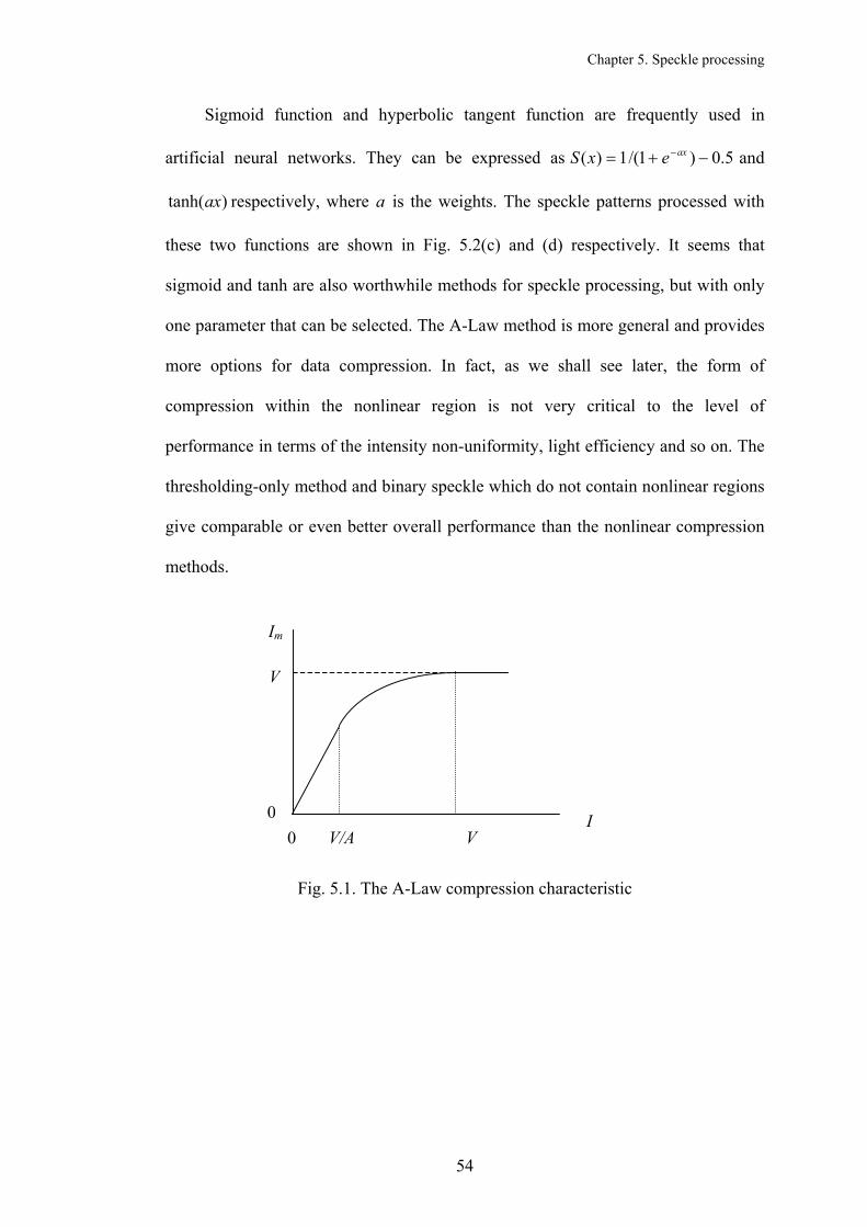
5.1 A-Law compression
A method known as A-Law compression [58] is commonly used in telephone
systems. The input signal I is divided into three regions and the output signal is given
by
>
≤≤+
+
≤≤+
=
)(for
)(for ln1
))/ln(1(
)(0for ln1
limitedVIV
clogarithmiVIAV
AVAIV
linearAVI
AAI
I m (5.1)
where V is the maximum value of the signal, and A is the compression coefficient.
The characteristic is shown in Fig. 5.1. For large values of A the characteristic is
predominantly logarithmic. When 1=A , the logarithmic region vanishes.
For the limited region, the intensities above the range [0, V] will be mapped to
the maximum value V, which is known as thresholding. The simulation of
thresholding can be easily performed in MATLAB by using function uint8(I/V*255)
or uint16(I/V*65535), where the values of input matrix I higher than V will be
brought back to 255 or 65535.
A MATLAB function compound (I, A, V, ‘A/compressor’) can be used to
implement logarithmic compression for the input signal I when the thresholding
operation is complete. The scalar A is the A-Law parameter, and V is the threshold
value. Example processed laser speckle images using A-Law compression are shown
in Fig. 5.2, where the threshold value V is set to ten times the mean of speckle
intensity S .
53
Chapter 5. Speckle processing
Sigmoid function and hyperbolic tangent function are frequently used in
artificial neural networks. They can be expressed as and
respectively, where a is the weights. The speckle patterns processed with
these two functions are shown in Fig. 5.2(c) and (d) respectively. It seems that
sigmoid and tanh are also worthwhile methods for speckle processing, but with only
one parameter that can be selected. The A-Law method is more general and provides
more options for data compression. In fact, as we shall see later, the form of
compression within the nonlinear region is not very critical to the level of
performance in terms of the intensity non-uniformity, light efficiency and so on. The
thresholding-only method and binary speckle which do not contain nonlinear regions
give comparable or even better overall performance than the nonlinear compression
methods.
5.0)1/(1)( −+= −axexS
)tanh(ax
00 V/A V
I
Im
V
Fig. 5.1. The A-Law compression characteristic
54

Chapter 5. Speckle processing
(a) A=10, S10=V (b) A=40, S10=V
(c) (d) 0002.0=a 0001.0=a
Fig. 5.2 Laser speckle patterns processed with (a) and (b): A-Law,
(c): sigmoid, (d): hyperbolic tangent
Applying A-Law processing to each individual reference speckle pattern
before the averaging process (2.18), new simulation results are obtained
and these are shown in Fig. 5.3. Compared with Fig. 3.6, it may be seen that the
image uniformity for a given number of frames is significantly improved. Or,
conversely, for a given image quality the number of frames can be reduced by about
50% when
)0,,( yxI ref
10=A and S10=V , as shown in Fig. 5.4. Fig. 5.5 shows a comparison
of the depth discrimination performance of the non-scanning arrangement using A-
Law processing and the conventional scanning system. Fig. 5.6 shows a comparison
of the average resolution measure FWHM obtained in conventional scanning and
with the A-Law processed non-scanning system. Compared with Fig. 4.7, it may be
55

Chapter 5. Speckle processing
seen that the non-scanning system with A-Law processing improves the lateral
resolution at small defocus. The improvement is not significant at large defocus
because the reference speckle patterns are no longer correlated with the fluorescence
frames generated at large defocus and the A-Law method becomes less effective. Fig.
5.7 shows a comparison of the linearity of the A-Law and scanning arrangements. No
significant deterioration of performance is observed using the A-Law processing.
(a) Grayscale images
56

Chapter 5. Speckle processing
(b) The same data as in (a) but shown as a slice along the central line of each row Fig. 5.3. Simulated images of a uniform fluorescent object with A-Law processing applied to the reference speckle patterns (A=10, S10=V )
Fig. 5.4. A plot of intensity nonuniformity σ against the number of frames averaged
57

Chapter 5. Speckle processing
Fig. 5.5. Comparison of depth discrimination property between scanning and non-scanning with A-Law processing ( 10=A , S10=V )
Fig. 5.6. Average FWHM of the nine peaks in the simulated image of a non-scanning confocal microscope with A-Law processing ( , 10=A S10=V ). The error bars indicate the standard deviation
58
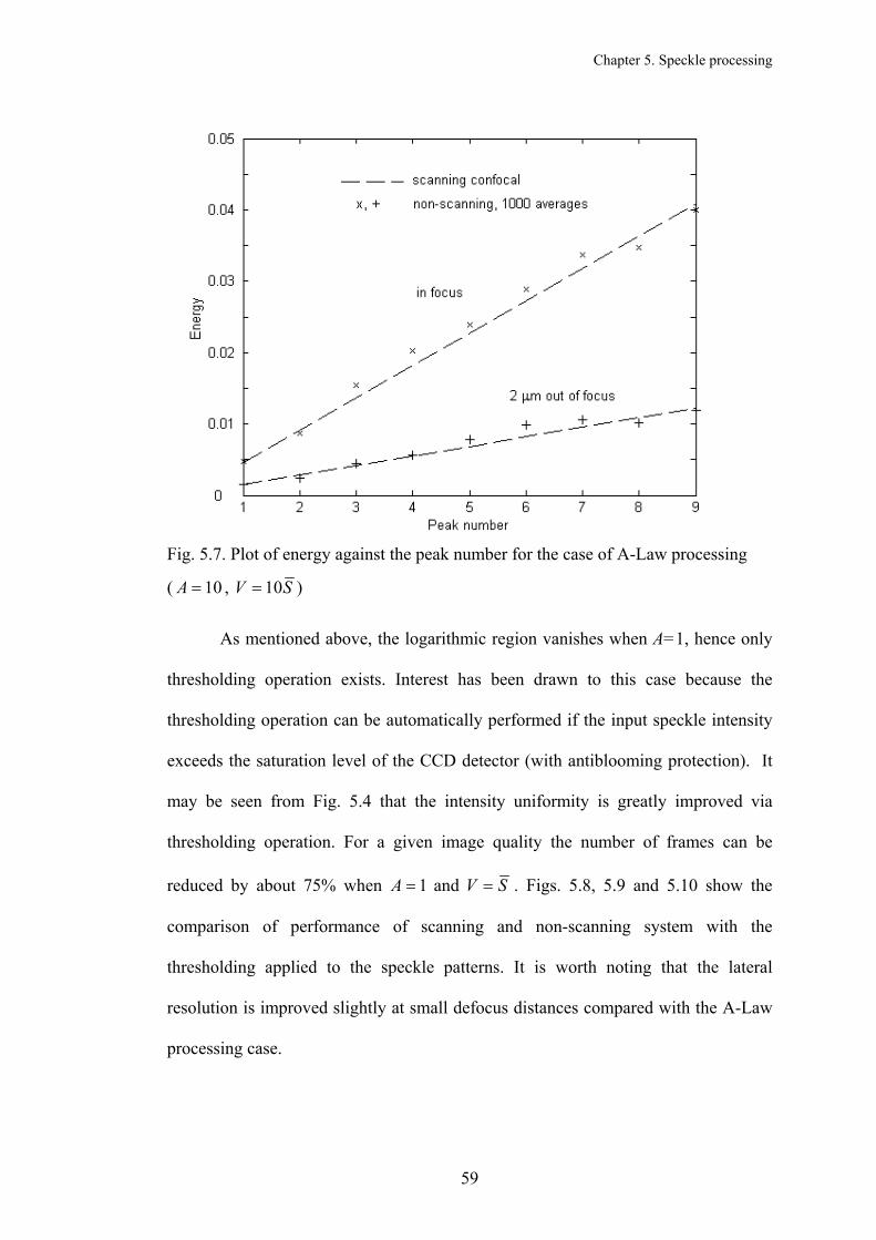
Chapter 5. Speckle processing
Fig. 5.7. Plot of energy against the peak number for the case of A-Law processing
( , 10=A S10=V )
As mentioned above, the logarithmic region vanishes when A=1, hence only
thresholding operation exists. Interest has been drawn to this case because the
thresholding operation can be automatically performed if the input speckle intensity
exceeds the saturation level of the CCD detector (with antiblooming protection). It
may be seen from Fig. 5.4 that the intensity uniformity is greatly improved via
thresholding operation. For a given image quality the number of frames can be
reduced by about 75% when 1=A and SV = . Figs. 5.8, 5.9 and 5.10 show the
comparison of performance of scanning and non-scanning system with the
thresholding applied to the speckle patterns. It is worth noting that the lateral
resolution is improved slightly at small defocus distances compared with the A-Law
processing case.
59

Chapter 5. Speckle processing
Fig. 5.8. Comparison of depth discrimination property between scanning and non-
scanning with thresholding operation ( 1=A , S=V )
Fig. 5.9. Average FWHM of the nine peaks in the simulated image of a non-scanning confocal microscope with thresholding operation ( , 1=A S=V ). The error bars indicate the standard deviation
60

Chapter 5. Speckle processing
Fig. 5.10. Plot of energy against the peak number for the case of thresholding 5.2 Binary speckle
A continuous laser speckle pattern can be represented by a binary one, shown in Fig.
5.11, in many applications, if a suitable threshold value is determined for a given
aperture, because the main features of the power spectral density of the speckle
intensity are maintained after a binarisation operation is performed [59].
(a) Threshold value S (b) Threshold value S5.1 Fig. 5.11. Binary speckle patterns
61

Chapter 5. Speckle processing
Fig. 5.12. Comparison of depth discrimination property between scanning and non-scanning with binary speckle (threshold value= S )
Fig. 5.13. Averaged FWHM of the nine peaks in the simulated image of a non-scanning confocal microscope with binarisation. The error bars indicate the standard deviation
62

Chapter 5. Speckle processing
Fig. 5.14. Plot of energy against the peak number for the case of binary speckle (threshold value = S )
By using binary speckle patterns the intensity non-uniformity can be reduced
by about a factor of 2 as shown in Fig. 5.4. Figs 5.12, 5.13 and 5.14 show the
comparison of performance of scanning and non-scanning system with binary
speckle patterns. No significant change in depth discrimination property and linearity
of the system is observed. However the FWHM values are widely distributed at
higher defocus distances.
Compared with A-Law compression and thresholding-only, binary speckle not
only reduces the number of frames effectively but also reduces the amount of digital
storage space. For example, transforming a speckle pattern of 256 grey levels into a
pattern of 2 levels results in an 8:1 savings in digital storage space. This is useful for
the real-time image processing which will be discussed in Chapter 7, as the speckle
patterns recorded from a CCD camera need to be transmitted to a miniature LCD and
reproduced on the LCD instantaneously. The use of binary speckle should reduce the
63

Chapter 5. Speckle processing
response time or may lead to the exploitation of binary optically addressed spatial
light modulator [60, 61].
5.3 Analysis
The above simulation of non-scanning confocal imaging with the application of
speckle processing shows that both the A-Law and binarisation operations have
significant positive influences on the intensity non-uniformity and the intensity non-
linearity, some degree of influences on the FWHM of the point spread function, but
no effect on the depth discrimination in terms of the performance evaluation criteria
considered. Since the simulation is performed based on the parameters chosen by
chance, it is therefore necessary to examine how the intensity non-uniformity σ and
the FWHM vary jointly with the compression coefficient A and the threshold value
V, so that optimum parameters may be determined by the compromise between σ and
FWHM. Note that σ also acts as a measure of light efficiency since by definition it is
inversely proportional to the mean of image intensity, and the ADL which acts as a
measure of the intensity nonlinearity can be represented by σ, since the intensity
nonlinearity arises actually from the intensity non-uniformity and both have the same
dependence on the number of frames as pointed out in section 4.2.
An analysis for this purpose is conducted and the results for the cases of
, , and binarisation operation are shown in Figs. 5.15 to 5.18
respectively. The FWHMs are calculated for the point object at two focal positions
(in focus and 2µm out of focus). It may be seen that optimum parameters can be
determined by making a compromise. For the case of A=1, or the thresholding-only
operation, the optimum threshold value appears between
1=A 10=A 20=A
>< S and . The >< S2
64

Chapter 5. Speckle processing
choice of compression coefficient A is not very critical to the level of performance.
The optimum threshold value for the case of A=10 or A=20 is the same which is
. For the binarisation case, the optimum threshold value should be < . A
summary of the above analysis is given in Table 5.1 where the crosses indicate the
corresponding optimal parameters.
>< S2 >S
Fig. 5.15 The relations of σ and FWHM with threshold value V (A=1)
65

Chapter 5. Speckle processing
Fig. 5.16. The relations of σ and FWHM with threshold value V (A=10)
Fig. 5.17. The relations of σ and FWHM with threshold value V (A=20)
66

Chapter 5. Speckle processing
Fig. 5.18. The relations of σ and FWHM with threshold value V (binary speckle)
A-Law
A V 1 10 20
Binary
<S> x
1.5<S> x
2<S> x x
5<S>
Table 5.1. Optimal parameters for speckle processing
It can be concluded that all the methods work at an acceptable standard when
optimal parameters are chosen. In the practical system the choice of method could be
made on the basis of which method is easier to implement.
67

Chapter 6. Experimental confirmation
6. Experimental confirmation
“Success is going from failure to failure without a loss of enthusiasm.”
Sir Winston Churchill, 1874-1965
A prototype optical bench system is constructed to demonstrate the practicality and
effectiveness of the non-scanning confocal microscopy idea.
6.1 Experimental arrangement
A schematic diagram of the experimental arrangement is shown in Fig. 6.1.
Illumination is from a laser beam passed through a rotating diffuser, a collimating
lens and an objective. The dichroic beamsplitter directs the beam to form a speckle
pattern throughout the specimen region. The fluorescent light from the object at a
longer wavelength is imaged via the lenses and the beamsplitter onto the CCD
camera. In this system, the fluorescence images and their corresponding illumination
speckle patterns are recorded separately. This requires that the diffuser “remember”
all the positions in a duty cycle and generate precisely the same sequence of speckle
patterns repetitively. A stepper motor is used for this purpose. At every diffuser
position, the camera takes a frame. A filter centred on the emission wavelength is
used for blocking unwanted laser light in the fluorescence image recording session.
In the speckle pattern recording session, the beamsplitter is replaced with a mirror
turned by 90 degrees and a diaphragm is added to generate the correct speckle size.
The experiment is aimed at demonstration of principle although the current
arrangement would be slower than conventional scanning systems.
68

Chapter 6. Experimental confirmation
mirror
diaphragm
s objective filter at fluorescent light
Cooled CCD camera
computer
diffu
dichroic beamsplitter
Dotted components: used in the spe
Dashed components: used in the flu
Solid components: used in both sess
Fig. 6.1. A schematic diagram of th
6.2 Apparatus
The apparatus which plays an important r
section.
6.2.1 Laser
A Sapphire 488-20 solid state laser sup
features of importance for this applicatio
fluorescent dyes work at this wavelength
specifications are given in Table 6.1 [62].
devices called Vertical External Cavity
conventional VECSELs, laser emission is d
Sapphire laser, in contrast, is optically pum
69
tube len
stepper motor
laser
ser collimating
attenuato
ckle pattern recording session
orescence image recording sessio
ions
e experimental arrangement
ole in the experiment is describe
plied by Coherent Inc was chos
n are the 488 nm wavelength
and the variable output power.
The Sapphire 488-20 belongs to a
Surface Emitting Lasers (VECS
riven (pumped) by electrical curr
ped. It comprises a semiconduct
specimen
lens
r
n
d in this
en. The
as many
Its main
class of
EL). In
ent. The
or pump

Chapter 6. Experimental confirmation
laser, focusing optics, a unique InGaAs quantum-well semiconductor that serves as a
gain medium and an output coupler, as illustrated in Fig. 6.2. Pump radiation from an
808 nm diode laser is focused on the OPS chip and absorbed by the quantum wells of
the chip, providing gain at the fundamental IR wavelength. With the inclusion of an
intra-cavity, nonlinear crystal, the infrared emission of the OPS chip is converted, via
second harmonic generation, to visible light at 488 nm. A remarkable property of
Sapphire is that the output is both single transverse mode (TEM00) and single
longitudinal mode (single frequency). In addition, Sapphire consumes 98% less input
power than argon iron lasers. It draws a maximum 60 W of electrical power, 50 W of
which goes to the thermoelectric cooler that stabilizes the resonator independent of
the environmental conditions. The remaining 10 W generates blue output. By
comparison, the air-cooled iron laser requires 1.0 to 1.5 kW of power.
Wavelength 488 ±2 nm
Coherence length >20 m
Output Power 1 ~ 20mW
Spatial Mode TEM00, M2 <1.1
Beam Asymmetry <1:1.1
Beam Diameter@ 1/e2 0.70 ±0.05 mm
Beam Divergence <1.2 mrad
Pointing Stability
(over 2 hours after warm-up and ±3°C) <30 µrad
Noise
20 Hz to 2 MHz
20 Hz to 20 kHz, peak-to-peak
<0.25%
<1%
Long-term Power Stability (2 hours, ±3°C) <2%
Polarization Ratio >100:1, vertical
Table 6.1 Laser specifications
70

Chapter 6. Experimental confirmation
Fig. 6.2. Sapphire resonator
(From the May 2001 issue of PHOTONICS SPECTRA © Laurin Publishing)
6.2.2 CCD camera
The ORCA cooled CCD camera supplied by Hamamatsu Photonics has low dark
noise and high quantum efficiency and is ideal for low-light level imaging. Its main
specifications and spectral response characteristics are given in Table 6.2 and Fig.
6.3 respectively [63].
Fig. 6.3. Spectral response characteristics
71
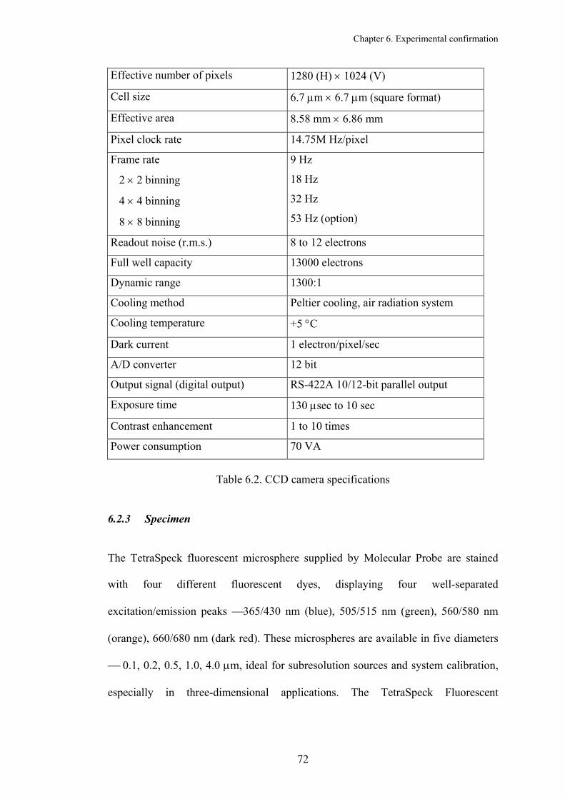
Chapter 6. Experimental confirmation
Effective number of pixels 1280 (H) × 1024 (V)
Cell size 6.7 µm × 6.7 µm (square format)
Effective area 8.58 mm × 6.86 mm
Pixel clock rate 14.75M Hz/pixel
Frame rate
2 × 2 binning
4 × 4 binning
8 × 8 binning
9 Hz
18 Hz
32 Hz
53 Hz (option)
Readout noise (r.m.s.) 8 to 12 electrons
Full well capacity 13000 electrons
Dynamic range 1300:1
Cooling method Peltier cooling, air radiation system
Cooling temperature +5 °C
Dark current 1 electron/pixel/sec
A/D converter 12 bit
Output signal (digital output) RS-422A 10/12-bit parallel output
Exposure time 130 µsec to 10 sec
Contrast enhancement 1 to 10 times
Power consumption 70 VA
Table 6.2. CCD camera specifications
6.2.3 Specimen
The TetraSpeck fluorescent microsphere supplied by Molecular Probe are stained
with four different fluorescent dyes, displaying four well-separated
excitation/emission peaks 365/430 nm (blue), 505/515 nm (green), 560/580 nm
(orange), 660/680 nm (dark red). These microspheres are available in five diameters
0.1, 0.2, 0.5, 1.0, 4.0 µm, ideal for subresolution sources and system calibration,
especially in three-dimensional applications. The TetraSpeck Fluorescent
72

Chapter 6. Experimental confirmation
Microspheres Size Kit (T-14792) includes a sample of each size, plus a mixture of
each size, mounted on six separate slides.
6.2.4 Filters
The dichroic beamsplitter is supplied by Omega Optical Inc. The spectra of the
dichroic beamsplitter is shown in Fig. 6.4. The emitter, supplied by Ealing Electro
Optics, has a central wavelength of 520 nm with a tolerance of ±10 nm.
Fig. 6.4. Spectra of the beamsplitter
6.2.5 Rotating diffuser
At least 500 different speckle patterns for each image recording session are required.
Such a great number of patterns are generated by a rotating diffuser which, driven by
a stepper motor through a gearbox, has a high resolution of up to 1000 steps per
degree. There are two types of speckle motion from a rotating diffuser [64]. If the
observation plane in the extreme near field of the illuminated area, speckle
translation will occur; the entire speckle pattern will move parallel to the motion of
the illuminated surface with little change in the shape or relative position of the
individual speckles. In the extreme far field, speckle boiling will occur; the speckles
will randomly evolve with no apparent displacement of the overall pattern. It is easy
73

Chapter 6. Experimental confirmation
to see from Fig. 6.1 that the speckle motion in our experiment just belongs to the first
type. In this case, the overall pattern at two consecutive diffuser positions appears to
move some distance without boiling. If the diffuser moves a distance smaller than the
illuminating spot, the two identical patterns may partly overlap within the field of
view. It is not clear whether this scenario will affect the averaging process, so the
diffuser is required to move a distance larger than the laser spot to avoid overlapping.
As the size of the laser spot is 0.7 mm and the disc is 120 mm in diameter, the
maximum number of frames within one turn will be limited to 120π/0.7≈538. For
convenience it is rounded to an integer of 500 by setting 720 steps for an angular
movement each time, which is 360/500 = 0.72°.
6.3 Principal parameters
The experimental system must meet the following requirements:
1. The Rayleigh resolution distance of the objective should be greater than the
size of fluorescent beads which are used as subresolution point sources
2. The numerical aperture of the objective is sufficiently large, as the light
emanating from the fluorescent beads is very weak
3. Each fluorescent bead should be magnified large enough so that its image
occupies a reasonable number of CCD pixels to satisfy the Nyquist sampling
condition (at least 2 pixels across the FWHM of a star image)
4. There are a reasonable number of beads within the field of view, preferably 10
or more, depending on the sample
Obviously the first requirement calls for a low-aperture objective and smaller beads
while the second calls for a high-aperture objective and larger beads. As a
compromise, we select the 4 µm fluorescent beads as the test specimen and a 5 time
74

Chapter 6. Experimental confirmation
objective with an NA of 0.12. Such an objective cannot resolve two 4 µm beads
separated 2 µm from each other when working in the type 1 (conventional) mode but
should be able to resolve them in the type 2 (confocal) mode. Given a magnification
of 20 which enables the image of a single bead to occupy 12 CCD pixels with a cell
size of 6.7 µm, the focal length of the tube lens is then determined. Note that the
image of the bead actually occupies 6 pixels because 2×2 binning∗ is used throughout
the experiment. This is equivalent to 7.5 pixels across the intensity PSF (a bit
oversampling). The principal parameters for the experimental system are listed in
Table 6.3.
Size of sample fluorescent beads 4 µm in diameter
Wavelength of laser light λ1 = 488 nm
Wavelength of fluorescence light λ2 = 520 nm
Numerical aperture of the objective NA = 0.12
Focal length of the objective f1 = 25.5 mm
Rayleigh resolution distance σ = 0.61λ2/NA = 2.64 µm
Speckle size on the object plane 1.22λ1/NA ≈ 5 µm
Focal length of the tube lens f2 = 500 mm
Magnification between the object and image planes M = f2/f1=19.61 ≈ 20
Aperture diameter of the diaphragm 2f1NA=6.12 mm
Field of view ≈ 430 µm × 340 µm
CCD resolution 640 × 512 pixels (2 × 2 binning)
Focal length of the collimating lens f3 = 30 mm
Angular movement of the diffuser 0.72°
Number of steps per revolution for the diffuser 500
Table 6.3. Principal parameters for the experimental system
∗ A way of increasing camera sensitivity by combining signals from multiple pixels, but this process reduces image resolution.
75
Chapter 6. Experimental confirmation
6.4 Light budget
A major problem experienced is the heavy loss of light due to the diffuser. With the
laser of 20 mW output power the incident power at the specimen is measured to be
only 0.6 mW which is not sufficient for fluorescence emission. A collimating lens is
therefore employed to converge the light scattered by the diffuser, thus increasing the
illumination power to 3 mW, and giving about 10-6 – 10-7 mW of emerging
fluorescent light at 520 nm emanating from the 4µm fluorescent bead specimen.
6.5 Image noise analysis
For the cooled CCD camera, thermal noise is not dominant, so noise in the image can
be considered as coming from two sources, readout noise and Poisson noise (shot
noise). From Table 6.2 the readout noise of the CCD camera can be assumed to be 20
electrons. The quantum efficiency of the camera is 50% according to Fig. 6.2. In the
fluorescence image recording session the CCD camera is exposed to the 4 µm
microsphere sample at a signal level of, presumably, 2×10⁻⁷ mW for 1 sec. Since 1
mW of light intensity at 500 nm is equivalent to 2×10¹⁵ photons/sec [65], the number
of photons absorbed at each pixel would be 400 (assuming an image of 1000×1000
pixels). This is just the case described in Ref. [16] from which a whole paragraph is
quoted as follows:
“In general terms, detector noise is most important at very low photon levels,
Poisson noise at higher levels. In a typical cooled CCD camera, the measurement
noise, mostly readout noise from the A/D converter in the camera, is about ten
electrons (r.m.s.) per pixel. This means that if many measurements of exactly the
same number of electrons were made, the standard deviation (root mean square
deviation from the mean value) would be ten. So, if exactly 100 electrons had
76

Chapter 6. Experimental confirmation
accumulated in a particular pixel in the array, there would be a probability of about
70% that the measured number would be between 90 and 110. The detective
quantum efficiency varies between 20% and 80% depending on the wavelength and
the CCD chip design. Let us assume 50%. This means that the detector noise is
equivalent to about 20 incident photons. Poisson noise arises because the emission
and detection of photons is a random process and fluctuates according to the Poisson
distribution. So if many measurements of a ‘uniform’ flux of photons were made
using a perfect measurement device, then the standard deviation of these
measurements would be given by the square root of the mean value. So, if the
detected number of photons is 100, we can regard this as a sample of a probability
distribution whose mean is 100 and whose standard deviation is 10. Thus at a signal
level of 400 photons, the Poisson noise would be 20 photons the same level as the
detector noise. At this signal level we could expect an r.m.s. noise-to-signal ratio of
around 7% (400 photons measured with 20 photons Poisson noise and the equivalent
of 20 photons detector noise since the two sources of noise are independent we
can add their contributions as the square root of the sum of their squares). With a
higher signal level, the shot noise would be greater than the (signal-independent)
detector noise.”
It should be noted that the above analysis does not take into account the
influence of external stray light, flare or light scattered by the elements of the optical
system and the light scattered through the object, which is thus cross talk between
object points. The former, which is constant in intensity over the detector, merely
serves to reduce contrast and can be subtracted from the detected signal. The latter in
the measured signal can be assumed to be uniformly distributed, so the intensity is
77

Chapter 6. Experimental confirmation
proportional to the area of the detector and also depends on the strength of the signal.
The quantifying of flare level is difficult and will not be discussed here.
6.6 Experimental results
6.6.1 Acquisition of raw images
The raw images of the specimen and the speckle pattern recorded with the
arrangement shown in Fig. 6.1 is different in their orientation, because in the
fluorescence image recording session the specimen is imaged inverted on the CCD
camera, while in the speckle recording session the image is erect. For this reason
either set of raw images must be flipped vertically prior to further processing. In
addition, in the speckle recording session the mirror must be accurately adjusted to
make sure that the corresponding points of the speckle pattern and the fluorescence
image are registered on the same pixel of the CCD camera, otherwise the fluorescent
spheres in the image do not look perfectly round. However it is very difficult to find
out whether a speckle pattern is correctly registered, as it looks completely different
from its corresponding fluorescence image. To solve this problem we replace the
fluorescent beads, when the fluorescence image recording session is completed, with
a uniform fluorescent microscope slide supplied by Omega Optical Inc., and record
an incoherent speckle pattern generated by this slide. This incoherent speckle pattern,
as shown in Fig. 6.5(a), looks blurry but bears a resemblance to the coherent one
shown in Fig. 6.5(b) and therefore can be used as a reference for judging by the eye
whether the coherent speckle pattern is correctly registered while the mirror is being
adjusted.
78

Chapter 6. Experimental confirmation
(a) Incoherent speckle pattern (b) Coherent speckle pattern
Fig. 6.5. The incoherent speckle pattern bears a resemblance to the coherent one
The CCD camera is controlled by the image acquisition software WASABI. By
means of the Time Lapse Recording function provided, a sequence of images can be
acquired easily and stored to the computer’s hard disk as digital data. The rotating
diffuser is controlled by an in-built script list that specifies all the actions required of
the stepper motor before or after each image is acquired. An individual raw image of
fluorescent beads taken with an exposure time of 1 sec and a corresponding speckle
pattern are shown in Fig. 6.6. The histograms in Fig. 6.7 clearly show a negative
exponential intensity distribution in the speckle pattern. Note that the maximum
value is equal to 4095 and the mean maxS S is equal to 620, giving S6.6max ≈S
rather than S10max ≈S as mentioned in subsection 3.5.1. This is because the
minimum intensity in the speckle pattern is at a level of about 210 rather than zero
due to the background noise. Since the recorded speckle pattern is from the extreme
near field of the diffuser, as mentioned in section 6.2.5, it should be noted that the
bright spots in Fig. 6.6(b) do not look very evenly distributed (the central portion
contains more bright spots than the surrounding) due to the surface irregularities of
the hand-made diffuser.
79

Chapter 6. Experimental confirmation
(a) Fluorescent beads (b) Speckle pattern
Fig. 6.6 An individual raw image (640×512×12)
(a) Linear histogram (b) Logarithmic histogram
Fig. 6.7 Histograms of the speckle pattern in Fig. 6.6(b), V , 4095= 625≈S
6.6.2 Postprocessed images and discussion
The recorded raw speckle patterns can be used to generate processed speckle, viz. A-
law compressed, intensity thresholded and binary speckle patterns as shown in Fig.
6.8 using the methods mentioned in Chapter 5.
A type 1 image of the 4 µm fluorescent microspheres can be obtained by
taking an average over 500 individual fluorescence images each illuminated with a
different speckle pattern. A series of such images at focal position of 0, 20 and 40
µm are shown in Figs 6.9(a) to (d) respectively. It may be seen that there is a
considerable amount of flare present in the images which comes mostly from
80

Chapter 6. Experimental confirmation
external stray light and light scattered by the elements of the optical system. Figs
6.9(e) to (h) show the non-scanning or type 2 images at the same focal positions
using equation (2.18) and averaging over 500 frames, giving an evident depth
discrimination property, enhanced lateral resolution and reduced effect of flare. Figs
6.10(a) to (h) show the type 2 images averaged with A-Law compressed speckle
patterns. Figs 6.11(a) to (h) show the type 2 images averaged with intensity
thresholded and binary speckle patterns respectively. Surface and profile plots of the
local regions illustrated in Figs 6.9 (a), 6.9(e), 6.10(a), 6.11(a) and 6.11(e) are shown
in Figs 6.12 (a), (b), (c), (d) and (e) respectively. In may be seen that the rightmost
double bead can hardly be resolved for the type 1 case, but is clearly resolved for the
type 2 case.
The effect of speckle processing on the processed images can be discerned
from the profile plots of Fig. 6.12, although the differences between the performance
of the A-Law processing and binarisation operation are small, as has been pointed
out in Section 5.3. The threshold values chosen for the images in Figs. 6.12(c), (d)
and (e) are 4095, 2047 and 0.3×4095, which are equivalent to S6.6 , S3.3 and S2
respectively. According to the blue curves in Figs. 5.16 to 5.19, their corresponding
intensity non-uniformity σ is read to be 0.07, 0.08 and 0.1 respectively. This means
that Fig. 6.12(c) has the best image quality in the sense that its intensity non-
uniformity σ is the lowest. Fig. 6.12(e) is worse than (c) and (d) since its intensity
non-uniformity σ is 0.1, but it is still better than (b) whose intensity non-uniformity
σ is around 0.14 according to the black curve of Fig. 5.4. This speculation has been
confirmed with the experimental results. It should be emphasized that all the methods
improve the image uniformity at an acceptable standard.
81

Chapter 6. Experimental confirmation
(a) A-law compressed, 10=A , 4095=V
(b) intensity thresholded, 1=A , 2047=V
(c) binary, threshold value = 0.3×4095
Fig. 6.8 Processed speckle patterns
82

Chapter 6. Experimental confirmation
(a) (e)
(b) (f)
(c) (g)
(d) (h) (a), (b), (c) and (d): type 1 images; (e), (f), (g) and (h): type 2 images
Fig. 6.9. Images of 4 micron fluorescent microspheres (640 × 512 × 12) at focal
positions of 0, 20, 40 and 60 µm
83

Chapter 6. Experimental confirmation
(a) (e) (b) (f) (c) (g) (d) (h) (a), (b), (c) and (d): A=10, V= 4095; (e), (f), (g) and (h): A=20, V=4095
Fig. 6.10 Images of 4 micron fluorescent microspheres (640 × 512 × 12) at focal
positions of 0, 20, 40 and 60 µm, averaged with A-Law compressed speckle
84

Chapter 6. Experimental confirmation
(a) (e) (b) (f) (c) (g) (d) (h)
(a), (b), (c) and (d): Thresholded, V= 2047 (e), (f), (g) and (h): Binary, V=0.3×4095
Fig. 6.11 Images of 4 µm fluorescent microspheres (640 × 512 × 12) at focal positions of 0, 20, 40 and 60 µm, averaged with thresholded and binary speckle respectively
85

Chapter 6. Experimental confirmation
(a)
(b)
(c)
(d)
(e)
(a): type 1, (b): type 2, (c): type 2 with A-law compression, (d): type 2 with
thresholding operation, (e): type 2 with binarisation operation
Fig. 6.12 Surface and profile plots of local regions
86

Chapter 6. Experimental confirmation
Fig. 6.13 Comparison of depth discrimination property
Fig. 6.13 shows a comparison of depth discrimination property between
theory and experiment. Note that the theoretical curve is obtained from a scanning
confocal system with a uniform planar object. It is reasonable to do so because
theoretically the non-scanning confocal microscope has the same 3-D optical transfer
function as a scanning one whose longitudinal frequency bandwidth is identical for
both the low and high transaxial frequency components. The intensity variation in a
non-scanning system accounts for a discrepancy of less than 10%.
The above experimental results exhibit excellent agreement with theory and
improved performance predicted by computer simulation. In particular, the results
confirm the dramatic effect of non-scanning microscope on the removal of additive
white noise present in each individual frame as mentioned in subsection 3.5.3.
87

Chapter 7. Real-time optical data processing
7. Real-time optical data processing As has been pointed out earlier, the arrangement described in the previous chapter is
slow in data collection and hence is unsuitable for imaging of biological tissue like
living cells. This chapter is devoted to an investigation of reduction in data collection
time by means of optical data processing and analogue frame averaging, because
optical data processing can be performed in real time and analogue frame averaging
can be implemented by taking a single CCD readout. To this end, a modified
experimental system is set up where a miniature transmissive liquid crystal display
(LCD) is employed to perform a real-time multiplication operation between two
individual frames. An LCD used in combination with an analogue CCD camera
behaves as an optically addressed spatial light modulator (OASLM) [66]. The
reason why such a configuration was adopted instead of simply using a commercial
OASLM is that the latter is too expensive. For example, the ENST Bretagne OASLM
with a frame rate of 1 KHz was priced at 10k euros in 2004. Of course, the cheaper
LCD used in our experiment has a low transmission of 22% and a low frame rate of
60 Hz, compared with those high-speed SLM devices whose frame rate can exceed 1
MHz, such as the Lenslet Ablaze SLM based on MQW GaAs technology [67]. A
problem associated with such a low transmission and low frame rate is that the LCD
will display a smeared image when using dynamic speckle patterns generated with a
rotating diffuser. This smearing effect will become serious with the increase in
rotating speed of the diffuser and will reduce the transmission of the LCD. Under
such circumstances the LCD will seriously block the weak fluorescent light coming
from the sample. Because of this limitation, it is required that the speckle patterns
change very slowly with time and the exposure time of the CCD camera be long
enough to allow the averaging process to complete. Although this will extend the
88
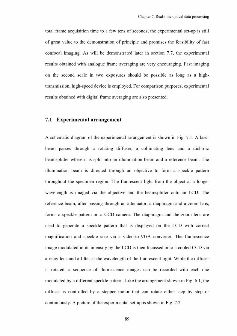
Chapter 7. Real-time optical data processing
total frame acquisition time to a few tens of seconds, the experimental set-up is still
of great value to the demonstration of principle and promises the feasibility of fast
confocal imaging. As will be demonstrated later in section 7.7, the experimental
results obtained with analogue frame averaging are very encouraging. Fast imaging
on the second scale in two exposures should be possible as long as a high-
transmission, high-speed device is employed. For comparison purposes, experimental
results obtained with digital frame averaging are also presented.
7.1 Experimental arrangement
A schematic diagram of the experimental arrangement is shown in Fig. 7.1. A laser
beam passes through a rotating diffuser, a collimating lens and a dichroic
beamsplitter where it is split into an illumination beam and a reference beam. The
illumination beam is directed through an objective to form a speckle pattern
throughout the specimen region. The fluorescent light from the object at a longer
wavelength is imaged via the objective and the beamsplitter onto an LCD. The
reference beam, after passing through an attenuator, a diaphragm and a zoom lens,
forms a speckle pattern on a CCD camera. The diaphragm and the zoom lens are
used to generate a speckle pattern that is displayed on the LCD with correct
magnification and speckle size via a video-to-VGA converter. The fluorescence
image modulated in its intensity by the LCD is then focussed onto a cooled CCD via
a relay lens and a filter at the wavelength of the fluorescent light. While the diffuser
is rotated, a sequence of fluorescence images can be recorded with each one
modulated by a different speckle pattern. Like the arrangement shown in Fig. 6.1, the
diffuser is controlled by a stepper motor that can rotate either step by step or
continuously. A picture of the experimental set-up is shown in Fig. 7.2.
89

Chapter 7. Real-time optical data processing
Fig. 7.1. A schematic diagram of the experimental arrangement
CCD camera
zoom lens cooled CCD camera
sample relay lens
DBS
r
Fig. 7.2. A picture of the experim
90
laser
diffuseLCD
ental set-up
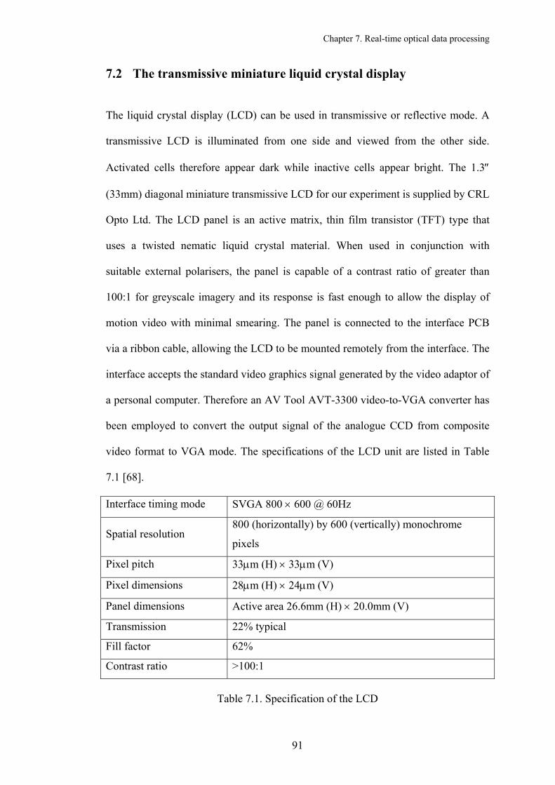
Chapter 7. Real-time optical data processing
7.2 The transmissive miniature liquid crystal display
The liquid crystal display (LCD) can be used in transmissive or reflective mode. A
transmissive LCD is illuminated from one side and viewed from the other side.
Activated cells therefore appear dark while inactive cells appear bright. The 1.3″
(33mm) diagonal miniature transmissive LCD for our experiment is supplied by CRL
Opto Ltd. The LCD panel is an active matrix, thin film transistor (TFT) type that
uses a twisted nematic liquid crystal material. When used in conjunction with
suitable external polarisers, the panel is capable of a contrast ratio of greater than
100:1 for greyscale imagery and its response is fast enough to allow the display of
motion video with minimal smearing. The panel is connected to the interface PCB
via a ribbon cable, allowing the LCD to be mounted remotely from the interface. The
interface accepts the standard video graphics signal generated by the video adaptor of
a personal computer. Therefore an AV Tool AVT-3300 video-to-VGA converter has
been employed to convert the output signal of the analogue CCD from composite
video format to VGA mode. The specifications of the LCD unit are listed in Table
7.1 [68].
Interface timing mode SVGA 800 × 600 @ 60Hz
Spatial resolution 800 (horizontally) by 600 (vertically) monochrome
pixels
Pixel pitch 33µm (H) × 33µm (V)
Pixel dimensions 28µm (H) × 24µm (V)
Panel dimensions Active area 26.6mm (H) × 20.0mm (V)
Transmission 22% typical
Fill factor 62%
Contrast ratio >100:1
Table 7.1. Specification of the LCD
91

Chapter 7. Real-time optical data processing
7.3 Principal parameters
In addition to the points to determine the system parameters discussed in Section 6.3,
a new factor that should be considered is the influence of the pixelated structure of
the LCD. Since the pixel size of the LCD is about five times that of the cooled CCD
camera, the image of the beads falling on the LCD has to be magnified by the same
amount to eliminate the effect on resolution. This suggests a change in the
magnification between the sample and the LCD from 20, set in the previous
experiment, to 100 and requires a subsequent increase in the focal length of the tube
lens to 2500 mm if the objective stays the same. Needless to say, the bench system
with a lens of such a long focal length will have to be a folded one and not look
respectable. For this reason, we keep the magnification unchanged at 20, which
results in the image of a single bead occupying about 2.4 LCD pixels with unwanted
dark grid pattern imposed due to the pixelated structure of the LCD. However, this
shortcoming is trivial and would be overcome if a high-resolution XGA (1024 × 768
pixels) LCD with a smaller pixel pitch of 18×18 µm could be used. The principal
parameters determined for the experiment are listed in Table 7.2.
92

Chapter 7. Real-time optical data processing
Size of sample fluorescent beads 4 µm in diameter
Wavelength of laser light λ1 = 488 nm
Wavelength of fluorescence light λ2 = 520 nm
Numerical aperture of the objective NA = 0.12
Focal length of the objective f1 = 25.5 mm
Rayleigh resolution distance σ = 0.61λ2/NA = 2.64 µm
Speckle size on the object plane 1.22λ1/NA ≈ 5 µm
Focal length of the tube lens f2 = 500 mm
Magnification between the object and LCD panel M1 = f2/f1=19.61 ≈ 20
Focal length of the relay lens f3 = 40 mm
Magnification between LCD and cooled CCD M2 = 1
Aperture diameter of the diaphragm 2f1NA=6.12 mm
Field of view ≈ 430 µm × 340 µm
CCD resolution 640 × 512 pixels (2 × 2 binning)
Focal length of the collimating lens f4 = 30 mm
Table 7.2. Principal parameters for the experiment
7.4 Optical data processing
Obviously, the ensemble average ⟩⋅⟨ SI in the first term of formula (2.18) can be
obtained by recording a sequence of individual LCD modulated images I and
then calculating the average. The following requirements must be met to ensure the
speckle pattern is correlated:
S⋅
Each image I is modulated with the speckle pattern S which is simultaneously
used to illuminate the sample
The position of the LCD panel must be precisely adjusted to allow the image I
to be accurately registered with the corresponding pixel locations on the LCD
panel
The modulated image formed at the cooled CCD detector can then be expressed as
93

Chapter 7. Real-time optical data processing
),(),(),( yxnyxSyxI + (7.1)
where n is the inevitable additive white noise. The LCD acts as an optical valve
whose liquid crystal cells are individually controlled by variable S to control the
amount of light transmitted. Obviously S should fall into the range of . 10 ≤≤ S
To obtain the second term ⟩⟩⟨⟨ SI in formula (2.18) in a suitable way, several
different approaches have been investigated:
1. Recording a sequence of individual fluorescence images without LCD
modulation and an additional sequence of speckle patterns. Inserting (7.1) into the
first term of the averaging formula (2.18) and (3.15) into the second term gives
(7.2) )1(0
1
⟩⟨−⟩⟨+=
⟩⟩⟨⟨−⟩⟩⟨⟨−⟩⟨+⟩⟨=
⟩⟩⟨+⟨−⟩+⟨=
SnISnSInIS
SnInISI
p
p
where is the ideal processed image. It is clear that the noise
cannot be removed because the intensity distribution in a speckle pattern obeys a
negative-exponential probability density function, its probable maximum intensity is
approximately ten times the value of its mean (see Section 3.5.1), hence
⟩⟩⟨⟨−⟩⟨= SIISI p0
1.0≈⟩S⟨ .
Figs. 7.3, 7.4 and 7.5 show the simulated averaged image with LCD modulation
, the averaged image without LCD modulation ⟩n+⟨IS ⟩+⟨ nI and the processed
image respectively. The simulated white noise with a mean equal to 40% of the
maximum signal level and a standard deviation of 2.5% of the mean is added to each
fluorescence frame. It may be seen that I is seriously masked by noise. Therefore
this approach is not usable.
1pI
0p
94

Chapter 7. Real-time optical data processing
Fig. 7.3. The averaged image with LCD modulation ⟨ ⟩+ nIS
Fig. 7.4. The averaged image without LCD modulation ⟩+⟨ nI
95

Chapter 7. Real-time optical data processing
Fig. 7.5. The processed image 1pI
2. Recording a sequence of individual fluorescence images without LCD
modulation and substituting a constant C for ⟩⟨S . The processed image then
becomes
(7.3)
In order to obtain the ideal image , we require
)1(
2
CnCIISCnCInIS
CnInISI p
−⟩⟨+⟩⟨−⟩⟨=⟩⟨−⟩⟨−⟩⟨+⟩⟨=
⟩+⟨−⟩+⟨=
0pI 1.0≈⟩⟨= S
1
C , but the noise cannot
be removed unless C . Apparently both conditions cannot be satisfied with the
same constant. Fig. 7.6 show the simulation result when
1=
=C . The processed image
obtained by subtracting 2pI ⟩+⟨ nI in Fig. 7.4 from ⟩+⟨ nIS
⟩
in Fig. 7.3 becomes
negative and definitely not a type 2 image although the noise has been completely
removed. The experimental results shown in Figs. 7.7, 7.8 and 7.9 confirm the
simulation very well. The modulated image +⟨ nIS is obtained with the LCD on,
96

Chapter 7. Real-time optical data processing
while the unmodulated image ⟩+⟨ nI is obtained with the LCD off, so that the
constant C . We conclude that this approach is unusable too. 1=
Fig. 7.6. The simulated processed image 2pI
97
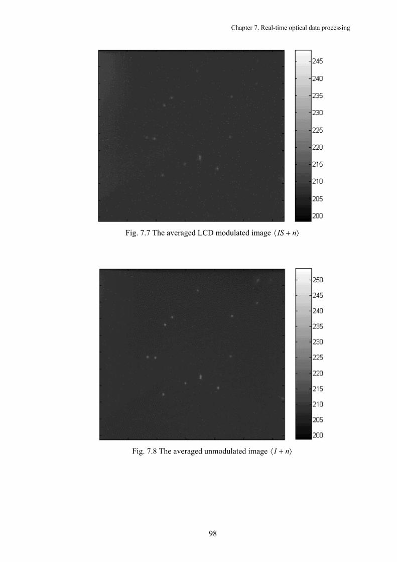
Chapter 7. Real-time optical data processing
Fig. 7.7 The averaged LCD modulated image ⟩+⟨ nIS
Fig. 7.8 The averaged unmodulated image ⟩+⟨ nI
98

Chapter 7. Real-time optical data processing
Fig. 7.9 The processed image 2pI
3. Recording a sequence of fluorescence images each modulated by an uncorrelated
speckle pattern S’. The processed image is then given by
(7.4) 0
3
''
'
p
p
ISIIS
nISnISnISnISI
=
⟩⟩⟨⟨−⟩⟨=⟩⟨+⟩⟨−⟩⟨+⟩⟨=
⟩+⟨−⟩+⟨=
Note that the ensemble average of the product of two uncorrelated random variables
is equal to the multiplication of their ensemble averages:
(7.5) ⟩⟩⟨⟨=⟩⟨ '' SIIS
and clearly,
(7.6) ⟩⟨=⟩⟨ SS '
The uncorrelated speckle pattern can be obtained by shifting the LCD laterally by a
small distance or that should exceed one speckle diameter, namely x∆ y∆
),(),(' yxxSyxS ∆−= (7.7)
99

Chapter 7. Real-time optical data processing
Fig. 7.10 shows the simulated averaged image ⟩+⟨ nIS ' obtained by shifting the LCD
horizontally by 20 pixels (equivalent to the speckle size). Fig. 7.11 shows the
processed image obtained using formula (7.4), and Fig. 7.12 the processed image
with its negative components suppressed. It is interesting to see that the image has a
satisfactory visual quality with most of the noise removed. Compared with
approaches 1 and 2, we conclude that approach 3 is a promising way forward, as it
can process data all-optically in two measurements taken with the LCD on and with
no need for knowledge of or ⟩⟨S ⟩⟨ 'S .
A downside of this approach is that the image intensity uniformity is a bit
worse than the two-detector system, and the noise level is relatively high. This is
because the correlated speckle ⟩⟨S in formula (2.18) is replaced with the
uncorrelated speckle ⟨ . According to the previous system performance
evaluation, the image intensity non-uniformity is dependent on the number of
averaging. The simulation results for this dependence is illustrated in Fig. 7.13 where
the first column shows the ideal images from a conventional microscope, the second
column shows the ideal images from a fluorescence scanning confocal microscope,
the third to six columns show the images obtained using formula 7.4, but averaged
over 500, 1000, 1500 and 2000 independent frames with additive white noise. It can
be seen that the intensity non-uniformity and the residual noise are reduced with the
increase in the number of averaging. From the discussion in Chapter 5, the intensity
uniformity can be improved through speckle processing. A comparison between
different speckle processing methods is shown in Fig. 7.14. Unfortunately the
unwanted intensity non-uniformity is about twice that of the two-detector
arrangement. The processing of binary speckle and thresholding are not significantly
effective, and the best candidate is the A-Law processing which gives an
⟩'S
100

Chapter 7. Real-time optical data processing
improvement of about 15%. A quantitative analysis of signal-to-noise ratio for the
non-scanning image in Fig. 7.13 was conducted using the same procedure as
described in section 3.5.3. The results (with the threshold value equal to 0.1) are
shown in Fig. 7.15. The in-focus image SNR of the SLM based system is between 5-
9, much lower than that of the two-detector system from Fig. 3.12.
Fig. 7.10. The averaged image modulated by uncorrelated speckle pattern ⟩+⟨ nIS '
101

Chapter 7. Real-time optical data processing
Fig.7.11. The processed image ⟩+⟨−⟩+⟨= nISnISI p '3
Fig. 7.12. The processed image with its negative components suppressed
102

Chapter 7. Real-time optical data processing
(a) Greyscale images
(b) Intensity distribution sliced along the central line of each panel Fig. 7.13. Simulation results using uncorrelated speckle processing
103

Chapter 7. Real-time optical data processing
Fig. 7.14. Intensity nonuniformity σ against the number of averaging
Fig. 7.15. The image signal-to-noise ratio in a SLM-based non-scanning system
104

Chapter 7. Real-time optical data processing
7.5 Experimental results with digital frame averaging
Encouraged by the results of the computer simulation presented in Section 7.4,
experiments were performed with 4µm fluorescent beads on the bench system shown
in Fig. 7.1. The experimental procedure includes two sessions for the specimen at
each focal position:
Record 500 frames of a field of 4µm fluorescent beads with each frame
modulated by LCD with a correlated speckle pattern
Move the LCD horizontally by about 100 µm, record 500 more frames with
each frame modulated with an uncorrelated speckle pattern
Measurements were taken for the object at 4 different focal positions. The
exposure time for each frame was set to 2 seconds. The recorded frames, stored on a
computer, were then processed using Eq. (7.4). An individual random laser speckle
pattern reproduced on the LCD is shown in Fig. 7.16. Its intensity distribution with a
negative-exponential characteristic is shown in Fig. 7.17. Figs 7.18 – 7.20 show the
averaged image modulated by correlated pattern ⟩+⟨ nIS , the averaged image
modulated by uncorrelated pattern ⟩+⟨ nIS ' and the processed image I respectively
when the object is in focus. Fig. 7.21 shows the processed image with the negative
components suppressed for the object at different focal positions. The experimental
results show evident agreement with theory and simulation except for the dark grid
pattern imposed due to the opaque mask between the LCD pixels. Another artefact is
that the beads in Fig. 7.20 look shadowy due to the fact that there is a small
displacement between the two averaged images. A zoom-in view of the bead
indicated with arrow in Fig. 7.20 is given in Fig. 7.22. The bead looks deformed as
3p
105

Chapter 7. Real-time optical data processing
shown in Fig. 7.23 after the negative components are removed. This problem will be
discussed later in section 7.6.
Fig. 7.16. The laser speckle pattern reproduced on the LCD
(a) Linear histogram (b) Logarithmic histogram
Fig. 7.17. Histograms of the speckle pattern in Fig. 7
106

Chapter 7. Real-time optical data processing
Fig. 7.18. The averaged image modulated by correlated pattern ⟨ ⟩+ nIS
Fig. 7.19. The averaged image modulated by uncorrelated pattern ⟨ ⟩+nIS '
107

Chapter 7. Real-time optical data processing
Fig. 7.20. The processed image 3pI
108

Chapter 7. Real-time optical data processing
(a) In focus (b) 20µm out of focus
(c) 40µm out of focus (d) 60µm out of focus
Fig. 7.21. Processed images (640 × 512 × 12) with the negative components
suppressed for the object at different focal positions
109

Chapter 7. Real-time optical data processing
Fig. 7.22. A zoom-in view of the bead indicated with arrow in Fig. 7.20
Fig. 7.23. A zoom-in view of the same bead as in Fig. 7.22 after the negative
components suppressed
110

Chapter 7. Real-time optical data processing
7.6 Image manipulation
As has been pointed out earlier, an artefact in the experimental result is that there is a
small displacement of bead location between the two averaged images, and the
amount of the displacement is different for the sample at different focal positions.
This problem may be caused by the misregistration of the fluorescence frame with
the corresponding pixel locations on the LCD panel during the measurement with
correlated speckle and by the shifting of the LCD between the two measurements, as
this scenario can be easily simulated by computer.
However this problem can be overcome by aligning the two averaged images
prior to the subtraction operation. A method for image alignment by cross-correlation
is introduced [69]. With this method the mismatch between two similar images can
be determined by measuring the peak offset from the origin of their cross-correlation.
But it is found that the method works only when no white noises exist in either image,
otherwise they cannot be subtracted away. Therefore, the processed image should be
expressed as
Tp ISISI ⟩⟨−⟩⟨= ' (7.8)
where denotes the ⟨ with a translational movement and it is assumed that
the averaged white noise has been removed from both images.
TIS ⟩⟨ ' ⟩'IS
⟩⟨n
To obtain the averaged white noise ⟩⟨n , 500 CCD frames were recorded with
the laser switched off. The histograms of an individual CCD frame and the averaged
frame are shown in Figs. 7.24 and 7.25 respectively. The standard deviation of the
averaged white noise has been reduced from 3.3 to 1, which implies that frame
averaging, or ensemble averaging, helps to reduce the white noise content. Figs. 7.26
and 7.27 show the images and ⟩⟨IS ⟩⟨ 'IS respectively where the noise has been ⟩⟨n
111

Chapter 7. Real-time optical data processing
subtracted. Figs. 7.28 and 7.29 show the subregions of Figs. 7.26 and 7.27 indicated
with arrows, from which we see that the bead is laterally displaced by a few pixels.
The cross-correlation c between images f and g can be written as
gfc ⊗= (7.9)
According to the correlation theorem, Eq. (7.9) in the Fourier space becomes
}{}{*}{ gFfFcF = (7.10)
where is the complex conjugate of . So we can easily obtain the cross-
correlation by taking the inverse Fourier transform of Eq. (7.10):
}{* fF }{ fF
(7.11) }}{}{*{1 gFfFFc −=
The calculated cross-correlation between the two subregions is shown in Fig.
7.30. The maximum of the cross-correlation is found at x=16, y=15, with an x-offset
of 3 pixels and a y-offset of 2 pixels from the origin (x=13, y=13). This means that
can be obtained by shifting image TIS ⟩⟨ ' ⟩⟨ 'IS 3 pixels upwards and 2 pixels to the
left. But, due to the pixelated structure of the LCD, the image intensities of the bead
in the subregions are not smoothly distributed, nor is their cross-correlation.
Therefore the assessed peak offset can be inaccurate. To avoid this problem, the
calculated cross-correlation needs to be smoothed prior to peak offset assessment.
The smoothed cross-correlation with a Gaussian kernel [70] is shown in Fig. 7.31.
Locations of the maxima of cross-correlation, smoothed cross-correlation and the
assessed movement for image ⟩⟨ 'IS for the object at different focal positions are
listed in Table 7.3.
The processed image for the object in focus obtained using Eq. (7.8) is shown
in Fig. 7.32, which does not look shadowy compared with Fig. 7.22. The images for
the specimen at different focal positions manipulated in the same way with negative
components suppressed are shown in Fig. 7.33. A zoom-in view of the bead
112

Chapter 7. Real-time optical data processing
indicated with arrow in Fig. 7.20 is given in Fig. 7.34. The bead reproduced by
removing the negative components is shown in Fig. 7.35 where no shape
deformation can be observed except the dark grid pattern imposed due to the
pixelated structure of the LCD. A zoom-in view of beads at different focal positions,
corresponding to Fig. 7.33, is shown in Fig. 7.36 where a depth discrimination
property is clearly displayed.
113
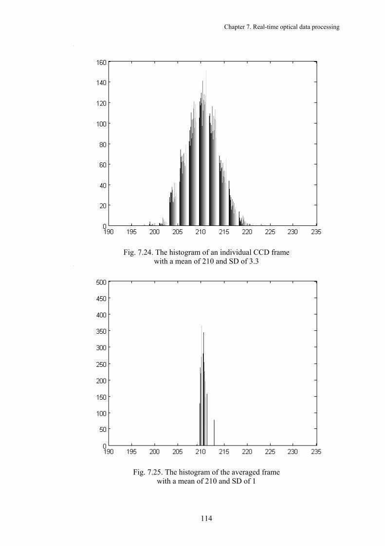
Chapter 7. Real-time optical data processing
Fig. 7.24. The histogram of an individual CCD frame
with a mean of 210 and SD of 3.3
Fig. 7.25. The histogram of the averaged frame
with a mean of 210 and SD of 1
114

Chapter 7. Real-time optical data processing
Fig. 7.26. The image ⟩⟨IS with ⟩⟨n removed
Fig. 7.27. The image ⟩⟨ 'IS with ⟩⟨n removed
115

Chapter 7. Real-time optical data processing
Fig. 7.28. The subregion of Fig. 7.26
Fig. 7.29. The subregion of Fig. 7.27
116

Chapter 7. Real-time optical data processing
Fig. 7.30. The cross-correlation between the two subregions
Fig. 7.31. Smoothed cross-correlation
117

Chapter 7. Real-time optical data processing
Focal position of the sample
(µm)
Centre of cross-
correlation
Location of maximum of
cross-correlation
Location of maximum of
smoothed cross-correlation
Assessed movement
0 x=13 y=13
x=16 y=15
x=15 y=15
2 pixels upwards 2 pixels to the left
20 x=13 y=13
x=13 y=14
x=14 y=14
1 pixel upwards 1 pixel to the left
40 x=13 y=13
x=13 y=13
x=13 y=13
No movement needed
60 x=18 y=18
x=14 y=19
x=14 y=19
4 pixels downwards
1 pixel to the left
Table 7.3 Assessment for image alignment
Fig. 7.32. The processed image Ip for the in-focus case with the image shifted
to the left by 2 pixels and then 2 pixels upwards
⟩⟨ 'IS
118

Chapter 7. Real-time optical data processing
(a) in focus (b) 20µm out of focus
(c) 40µm out of focus (d) 60µm out of focus
Fig. 7.33. The processed image with the negative components suppressed pI
119
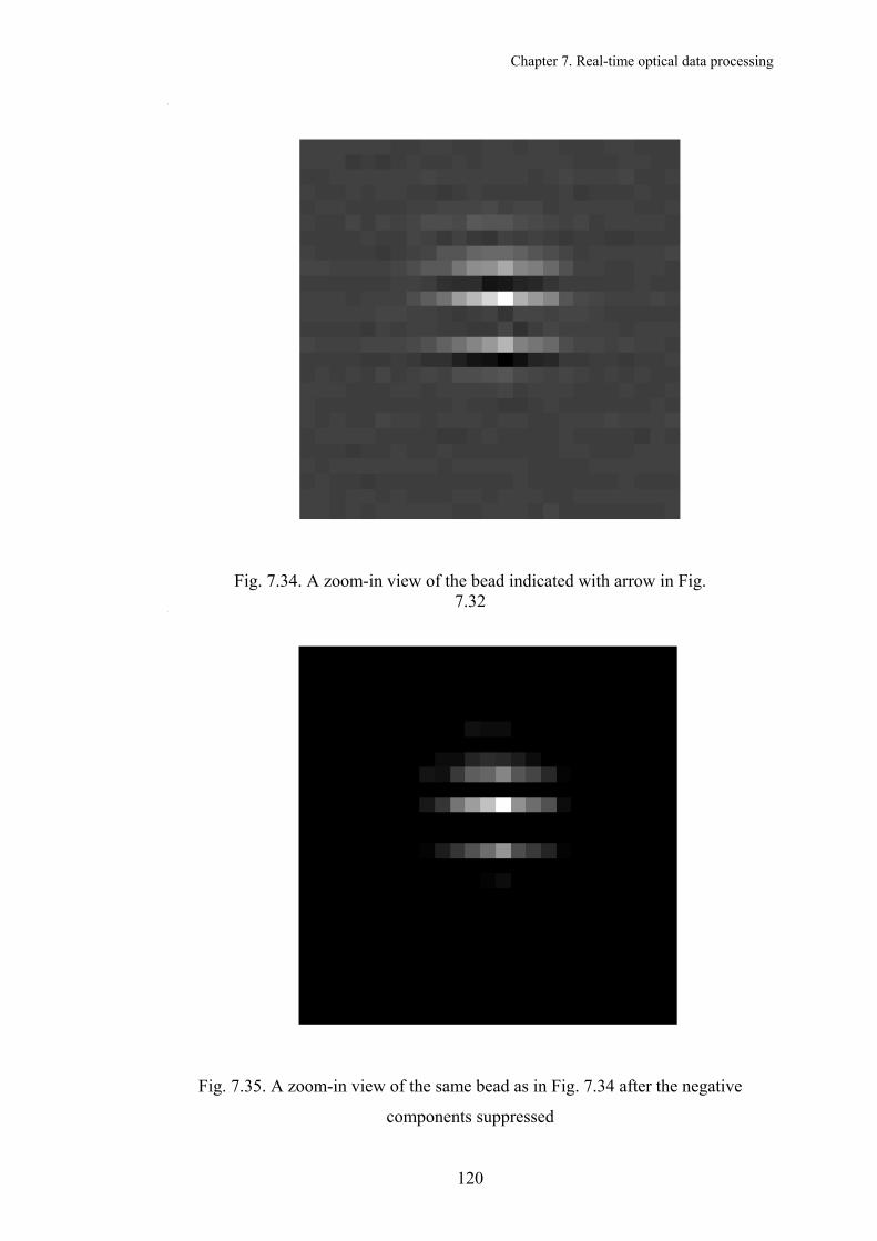
Chapter 7. Real-time optical data processing
Fig. 7.34. A zoom-in view of the bead indicated with arrow in Fig.
7.32
Fig. 7.35. A zoom-in view of the same bead as in Fig. 7.34 after the negative
components suppressed
120

Chapter 7. Real-time optical data processing
(a) In focus (b) 20 µm out of focus
(c) 40 µm out of focus (d) 60 µm out of focus
Fig. 7.36. A zoom-in view of beads at different focal positions
121

Chapter 7. Real-time optical data processing
7.7 Experimental results with averaging by CCD charge
accumulation
An experiment based on frame averaging by CCD charge accumulation or the two-
shot scheme was also conducted. Considering the low frame rate of the LCD, we set
the stepper motor speed to 150 steps/sec. The exposure time of the cooled CCD
camera was set to 10 seconds, during which time the diffuser rotates by 1.5°. The
speed of the speckle patterns moving vertically on the LCD panel was calculated to
be 2.6 mm/sec. The LCD was shifted vertically by 100 microns between the two
CCD readouts, because the speckle patterns change by far slower in the horizontal
direction than in the vertical direction, and a horizontal shift will not make
significant difference between the two measurements. The averaged frames and the
processed image are shown in Figs. 7.37. The images of the beads at focal positions
of 0µm, 20µm, 40µm and 60µm with and without image manipulation are shown in
Figs 7.38. A frame with the laser switched off is also recorded to obtain an image of
white noise for image manipulation. The processed images with the negative
components suppressed are shown in Fig. 7.39. A corresponding zoom-in view of
beads at different focal positions is shown in Fig.7.40 where a depth discrimination
property is clearly displayed. Compared with the experimental results with digital
frame averaging shown in Fig. 7.36, the averaging scheme by CCD charge
accumulation gives a very similar result but requires capturing only two frames so
that the data collection time can be reduced dramatically.
122

Chapter 7. Real-time optical data processing
(a) In focus (e) In focus
(b) 20 µm out of focus (f) 20 µm out of focus (c) 40 µm out of focus (g) 40 µm out of focus (d) 60 µm out of focus (h) 60 µm out of focus
Fig. 7.37. The images averaged by CCD charge accumulation (a)-(d): nIS + , (e)-(h): nIS +'
123

Chapter 7. Real-time optical data processing
(a) In focus (e) In focus, 1 pixel down (b) 20 µm out of focus (f) 20 µm out of focus, 1 pixel up (c) 40 µm out of focus (g) 40 µm out of focus, 1 pixel up (d) 60 µm out of focus (h) 20 µm out of focus, 1 pixel up
Fig. 7.38. The processed images (a)-(d): without image manipulation, (e)-(h): with image manipulation
124

Chapter 7. Real-time optical data processing
(a) In focus (e) In focus, 1 pixel down (b) 20 µm out of focus (f) 20 µm out of focus, 1 pixel up (c) 40 µm out of focus (g) 40 µm out of focus, 1 pixel up (d) 60 µm out of focus (h) 60 µm out of focus, 1 pixel up
Fig. 7.39. The processed image with the negative components suppressed (a)-(d): without image manipulation, (e)-(h): with image manipulation
125

Chapter 7. Real-time optical data processing
(a) in focus (b) 20 µm out of focus (c) 40 µm out of focus (d) 60 µm out of focus
Fig. 7.40. A zoom-in view of beads at different focal positions
126

Chapter 8. Conclusion and further work
8. Conclusion and further work
“The three things that are most essential to achievement are common sense, hard
work and stick-to-it-iv-ness.....”
Thomas Edison, 1847 – 1931
Fluorescence microscopy is the commonest approach for studying molecular
organisations and tissue structures. For anyone new to this area, however, it can be
difficult to decide which techniques or equipment to try: wide-field microscopy,
scanning confocal, or spinning disk confocal? When selecting which system to use
for imaging a sample, one should consider a few things: What spatial resolution is
required? Is the process to be observed fast or slow? Is the sample thick or thin? You
also need to consider some further questions: Is the sample subject to
photobleaching? What is the appropriate illumination intensity to avoid sample
damage? In many cases, no single microscope system will be best, and compromises
will have to be made. A strong demand of biologists for imaging their different
samples resulted in developments of new imaging techniques such as structured-light
illumination, 4Pi confocal microscopy, two-photon excitation microscopy, to name
just a few. Speckle-illuminated non-scanning fluorescence confocal microscopy, is a
novel method for obtaining images with the enhanced resolution and optical
sectioning properties of a confocal microscope but avoids the complexity of a
scanning system and potentially may avoid the long frame times associated with the
scanning process. This method has been investigated by experiment and computer
simulations, and the implementation of this method based on two different optical
arrangements is presented in this thesis. This chapter will summarize the conclusions
127
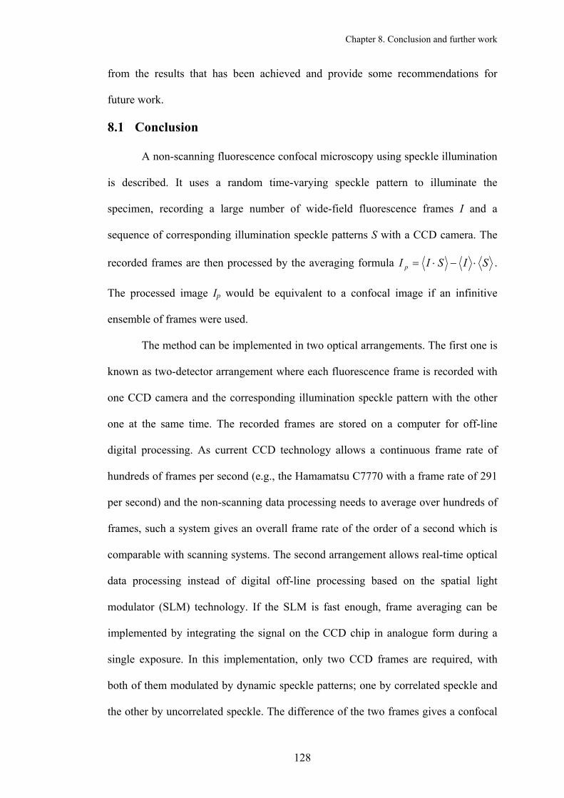
Chapter 8. Conclusion and further work
from the results that has been achieved and provide some recommendations for
future work.
8.1 Conclusion
A non-scanning fluorescence confocal microscopy using speckle illumination
is described. It uses a random time-varying speckle pattern to illuminate the
specimen, recording a large number of wide-field fluorescence frames I and a
sequence of corresponding illumination speckle patterns S with a CCD camera. The
recorded frames are then processed by the averaging formula SISIp ⋅−⋅=I .
The processed image Ip would be equivalent to a confocal image if an infinitive
ensemble of frames were used.
The method can be implemented in two optical arrangements. The first one is
known as two-detector arrangement where each fluorescence frame is recorded with
one CCD camera and the corresponding illumination speckle pattern with the other
one at the same time. The recorded frames are stored on a computer for off-line
digital processing. As current CCD technology allows a continuous frame rate of
hundreds of frames per second (e.g., the Hamamatsu C7770 with a frame rate of 291
per second) and the non-scanning data processing needs to average over hundreds of
frames, such a system gives an overall frame rate of the order of a second which is
comparable with scanning systems. The second arrangement allows real-time optical
data processing instead of digital off-line processing based on the spatial light
modulator (SLM) technology. If the SLM is fast enough, frame averaging can be
implemented by integrating the signal on the CCD chip in analogue form during a
single exposure. In this implementation, only two CCD frames are required, with
both of them modulated by dynamic speckle patterns; one by correlated speckle and
the other by uncorrelated speckle. The difference of the two frames gives a confocal
128

Chapter 8. Conclusion and further work
image. Developments in novel SLM structures, such as digital micromirror device
(DMD) [71, 72] and multiple quantum well (MQW) SLMs [73], have led to devices
with array sizes exceeding 256×256 and frame rates of 10 ∼ 100 KHz. Fast scanless
confocal imaging on the sub-second scale should be possible.
The effects of some important factors such as shot noise, Gaussian white
noise and quantisation error from a CCD detector on the non-scanning system were
investigated by simulation. The image signal-to-noise ratio for a multipoint object
was calculated using Murray’s procedure. It is shown that the in-focus image SNR of
the two-detector arrangement is between 30–70 for the frame number between 500–
2000, while the SLM based digital-averaging arrangement gives a SNR between 5-9.
For quantitative performance evaluation, several criteria were established in terms of
intensity non-uniformity, intensity non-linearity, depth discrimination property and
lateral resolution. The simulated behaviour of system was investigated against these
criteria. It is shown that the non-scanning system offers the same imaging response
as a scanning confocal system in the sense of depth discrimination property and
improved lateral resolution, except for a 10% image intensity variation with the two-
detector system and 20% with the SLM based system.
To reduce the number of frames required, some methods such as A-Law
compression and binary speckle were introduced to improve the efficiency of the
averaging process. The simulation results show that these methods can effectively
reduce the frame number by 50% for the two-detector system and 15% for the SLM
based system without any adverse effects on the performance assessed against the
same criteria.
Confocal imaging of 4µm fluorescent microspheres without a raster scan has
been realised on a self-built optical bench system. Since there is only one digital
129

Chapter 8. Conclusion and further work
CCD camera available, the two-detector experiment is implemented by using a
stepper motor and recording the fluorescent frames and the speckle frames
separately. The experimental results agree with simulation very well. It is shown that
the non-scanning system offers satisfactory image quality and good background
rejection. The SLM based experimental system uses a CCD camera in combination
with a transmissive LCD to operate as a OASLM. Frame averaging is performed in
two ways: digital frame averaging and analogue averaging by CCD charge
accumulation. Because of the low frame rate of the LCD used, analogue averaging is
accomplished by using slow time-varying speckle patterns and prolonged CCD
exposure time. The results obtained with the two averaging methods are very similar
and both show clear confocal properties. Since the SLM based system performs data
processing all-optically, the data collection time can be significantly reduced.
No matter which system is used, an important point that needs attention is
that the fluorescent frame and the corresponding speckle pattern must be correctly
registered with the CCD pixels, otherwise there would be a mismatch between the
two frames and the resulting image would show a shadow effect. However it has
been shown that this mismatch can be corrected automatically by calculating the
cross-correlation of the two frames.
In a few words, speckle-illuminated fluorescence microscopy offers several
advantages compared to the established scanning and non-scanning methods:
1. The same axial and lateral spatial resolution as the CSM
2. No need for a scanning apparatus
3. No need for a pinhole
4. Since the method is truly wide-field, it is less susceptible to photobleaching
because the light is not focused and the excitation density is much smaller [74]
130

Chapter 8. Conclusion and further work
5. The two-detector arrangement equipped with ordinary video CCD cameras has
an extremely simple structure. It can be used in place of conventional CSMs
when imaging speed is not essential
The principal disadvantages of this method compared to others is that
1. The illumination efficiency is low, about 15%, due to the use of the diffuser
2. There is a 10 – 20% unwanted variation in intensity levels
3. Not suitable for two-photon excitation
8.2 Further work
There is clearly a great deal of work yet to be done in order to develop a
sophisticated instrument on the basis of progress made to date. The issues to be
addressed include:
Current experiments are restricted to low-aperture case. It would be useful
and interesting to model high-aperture non-scanning confocal imaging using vector
theory which is outlined in section 2.12. Experiments could be made with high NA
objectives and standard submicron fluorescent beads.
It would be worthwhile to investigate other methods, such as sigmoid or tanh
function, for speckle processing.
As mentioned in section 6.2.5, there are two types of speckle motion from a
rotating diffuser: translation and boiling. The current simulation is restricted to the
boiling type. However the true case in a SLM based system is the translation type. It
would be useful if such a speckle motion could be modelled.
Whether a fast spatial light modulator is available will be crucial to the
survival of our research on fast confocal imaging with the SLM based system.
Recent literature survey shows that digital micromirror device (DMD) might be
131

Chapter 8. Conclusion and further work
feasible for our application. The DMD technology was perfected and commercialised
over the last decade. One of the advantages of DMD is that it can modulate light
independently of wavelength due to its simple reflective operation. The DMD has a
light modulator efficiency in the range of 65%. Binary frame rates up to 9,700
frames /second can be achieved for full array (1024x768) operation. LCDs are also
widely used SLMs and may be either transmissive or reflective, but do not have the
speed, precision or broadband capability that the DMD boasts. Commercial MQW
SLMs working at visible bands are still not available. A possible implementation of
two-shot scanless confocal microscopy using speckle illumination and the DMD for
optical data processing is illustrated in Fig. 8.1. One can expect a new optical
imaging technique to emerge!
CCD
DMD
PC CCD
source
diffuser
specimen
Fig. 8.1. Schematic representation of a speckle-illuminated non-scanning
fluorescence microscope using the DMD for optical data processing
132

Bibliography
Bibliography 1. M. Minsky, Memoir on Inventing the Confocal Scanning Microscope.
Scanning, 1988. 10(4): p. 128-138.
2. W.B. Amos, J.G. White, and M. Fordham, Use of Confocal Imaging in the
Study of Biological Structures. Applied Optics, 1987. 26(16): p. 3239-3243.
3. S.W. Paddock, ed. Confocal Microscopy Methods and Protocols. Methods in
Molecular Biology, ed. J.M. Walker. Vol. 122. 1999, Humana Press: Totowa,
New Jersey.
4. W.B. Amos and J.G. White, How the Confocal Laser Scanning Microscope
entered Biological Research. Biology of the Cell, 2003. 95(6): p. 335-342.
5. D.A. Agard, Y. Hiraoka, P. Shaw, and J.W. Sedat, Fluorescence Microscopy
in 3 Dimensions. Methods in Cell Biology, 1989. 30: p. 353-377.
6. S.J. Wright and G. Schatten, Confocal Fluorescence Microscopy and 3-
Dimensional Reconstruction. Journal of Electron Microscopy Technique,
1991. 18(1): p. 2-10.
7. M.J. Cole, J. Siegel, S.E.D. Webb, R. Jones, K. Dowling, M.J. Dayel, D.
Parsons-Karavassilis, P.M.W. French, M.J. Lever, L.O.D. Sucharov, M.A.A.
Neil, R. Juskaitis, and T. Wilson, Time-domain whole-field fluorescence
lifetime imaging with optical sectioning. Journal of Microscopy-Oxford,
2001. 203: p. 246-257.
8. D.J. Stephens and V.J. Allan, Light microscopy techniques for live cell
Imaging. Science, 2003. 300(5616): p. 82-86.
9. M.R. Young, S.H. Jiang, R.E. Davies, J.G. Walker, E.R. Pike, and M.
Bertero, Experimental confirmation of superresolution in coherent confocal
133
Bibliography
scanning microscopy using optical masks. Journal of Microscopy-Oxford,
1992. 165: p. 131-138.
10. Roy Pike, Superresolution in fluorescence confocal microscopy and in DVD
optical storage, in Confocal and Two-photon Microscopy, A. Diaspro, Editor.
2002, John Wiley and Sons: New York.
11. E.R. Pike and S.H. Jiang, Ultrahigh-resolution optical imaging of colloidal
particles. Journal of Physics-Condensed Matter, 2002. 14(33): p. 7749-7756.
12. Roy Pike, Deeph Chana, Pelagia Neocleous, and Shihong Jiang,
Superresolution in scanning optical systems, in Optical Imaging and
Microscopy, Peter Torok and F.-J. Kao, Editors. 2003, Springer: Berlin.
13. H. Tadakuma, J. Yamaguchi, Y. Ishihama, and T. Funatsu, Imaging of single
fluorescent molecules using video-rate confocal microscopy. Biochemical
and Biophysical Research Communications, 2001. 287(2): p. 323-327.
14. X. Michalet, A.N. Kapanidis, T. Laurence, F. Pinaud, S. Doose, M.
Pflughoefft, and S. Weiss, The power and prospects of fluorescence
microscopies and spectroscopies. Annual Review of Biophysics and
Biomolecular Structure, 2003. 32: p. 161-182.
15. J. Zimmermann, A. van Dorp, and A. Renn, Fluorescence microscopy of
single molecules. Journal of Chemical Education, 2004. 81(4): p. 553-557.
16. P.J. Shaw, Introduction to confocal Microscopy, in Light Microscopy in
Biology, A.J. Lacey, Editor. 1999, Oxford University Press: New York. p. 45-
71.
17. C.J.R. Sheppard, X. Gan, M. Gu, and M. Roy, Signal-to-noise in confocal
microscopes, in Handbook of biological confocal microscopy, J.B. Pawley,
Editor. 1995, Plenum Press: New York. p. 363-371.
134

Bibliography
18. J.R. Swedlow, K. Hu, P.D. Andrews, D.S. Roos, and J.M. Murray, Measuring
tubulin content in Toxoplasma gondii: A comparison of laser-scanning
confocal and wide-field fluorescence microscopy. Proceedings of the National
Academy of Sciences of the United States of America, 2002. 99(4): p. 2014-
2019.
19. LSM 510 and LSM 510 META Laser Scanning Microscopes, Operating
Manual, Release 3.2, Carl Zeiss, 2002
20. M. Petran, M. Hadravsk, M.D. Egger, and R. Galambos, Tandem-scanning
reflected-light microscope. Journal of the Optical Society of America, 1968.
58(5): p. 661.
21. H. Ishida, C. Genka, Y. Hirota, H. Nakazawa, and W.H. Barry, Formation of
planar and spiral Ca2+ waves in isolated cardiac myocytes. Biophysical
Journal, 1999. 77(4): p. 2114-2122.
22. A. Ichihara, T. Tanaami, H. Ishida, and M. Shimizu, Confocal fluorescent
microscopy using a Nipkow scanner, in Fluorescent and Luminescent Probes,
W.T. Mason, Editor. 1999, Academic Press: London.
23. Visitech International. Available at: <http://www.visitech.co.uk> [5 Jan
2005]
24. M.G.L. Gustafsson, D.A. Agard, and J.W. Sedat, (IM)-M-5: 3D widefield
light microscopy with better than 100 nm axial resolution. Journal of
Microscopy-Oxford, 1999. 195: p. 10-16.
25. M.G.L. Gustafsson, Surpassing the lateral resolution limit by a factor of two
using structured illumination microscopy. Journal of Microscopy-Oxford,
2000. 198: p. 82-87.
135

Bibliography
26. J.T. Frohn, H.F. Knapp, and A. Stemmer, True optical resolution beyond the
Rayleigh limit achieved by standing wave illumination. Proceedings of the
National Academy of Sciences of the United States of America, 2000. 97(13):
p. 7232-7236.
27. J.T. Frohn, H.F. Knapp, and A. Stemmer, Three-dimensional resolution
enhancement in fluorescence microscopy by harmonic excitation. Optics
Letters, 2001. 26(11): p. 828-830.
28. R. Fedosseev, Y. Belyaev, J. Frohn, and A. Stemmer, Structured light
illumination for extended resolution in fluorescence microscopy. Optics and
Lasers in Engineering, 2005. 43(3-5): p. 403-414.
29. B. Bailey, D.L. Farkas, D.L. Taylor, and F. Lanni, Enhancement of Axial
Resolution in Fluorescence Microscopy by Standing-Wave Excitation.
Nature, 1993. 366(6450): p. 44-48.
30. F. Lanni and B. Bailey, Standing -wave excitation for fluorescence
microscopy. Trends in Cell Biology, 1994. 4: p. 262-265.
31. B. Bailey, V. Krishnamurthi, D.L. Farkas, D.L. Taylor, and F. Lanni, Three-
dimensional imaging of biological specimens with standing wave
fluorescence microscopy. Proceedings of SPIE, 1994. 2184: p. 208-213.
32. V. Krishnamurthi, B. Bailey, and F. Lanni, Image processing in 3-D
standing-wave fluorescence microscopy. Proceedings of SPIE, 1994. 2655: p.
18-25.
33. M.A.A. Neil, R. Juskaitis, and T. Wilson, Method of obtaining optical
sectioning by using structured light in a conventional microscope. Optics
Letters, 1997. 22(24): p. 1905-1907.
136

Bibliography
34. M.A.A. Neil, R. Juskaitis, and T. Wilson, Real time 3D fluorescence
microscopy by two beam interference illumination. Optics Communications,
1998. 153(1-3): p. 1-4.
35. M.A.A. Neil, A. Squire, R. Juskaitis, P.I.H. Bastiaens, and T. Wilson, Wide-
field optically sectioning fluorescence microscopy with laser illumination.
Journal of Microscopy-Oxford, 2000. 197: p. 1-4.
36. S.E.D. Webb, Y. Gu, S. Leveque-Fort, J. Siegel, M.J. Cole, K. Dowling, R.
Jones, P.M.W. French, M.A.A. Neil, R. Juskaitis, L.O.D. Sucharov, T.
Wilson, and M.J. Lever, A wide-field time-domain fluorescence lifetime
imaging microscope with optical sectioning. Review of Scientific
Instruments, 2002. 73(4): p. 1898-1907.
37. M.G. Somekh, C.W. See, and J. Goh, Wide field amplitude and phase
confocal microscope with speckle illumination. Optics Communications,
2000. 174(1-4): p. 75-80.
38. J.G. Walker, Non-scanning confocal fluorescence microscopy using speckle
illumination. Optics Communications, 2001. 189(4-6): p. 221-226.
39. S.H. Jiang and J.G. Walker, Experimental confirmation of non-scanning
fluorescence confocal microscopy using speckle illumination. Optics
Communications, 2004. 238(1-3): p. 1-12.
40. S. Jiang and J.G. Walker, Non-scanning fluorescence confocal microscopy
using speckle illumination and optical data processing. Optics
Communications, 2005. 256(1-3): p. 35-45.
41. E. Wang, C.M. Babbey, and K.W. Dunn, Performance comparison between
the high-speed Yokogawa spinning disc confocal system and single-point
137

Bibliography
scanning confocal systems. Journal of Microscopy-Oxford, 2005. 218: p. 148-
159.
42. M.G. Gustafsson, Extended resolution fluorescence microscopy. Current
Opinion in Structrural Biology, 1999. 9(5): p. 627-634.
43. L.H. Schaefer, D. Schuster, and J. Schaffer, Structured illumination
microscopy: artefact analysis and reduction utilizing a parameter
optimization approach. Journal of Microscopy-Oxford, 2004. 216: p. 165-
174.
44. C.J.R. Sheppard and D.M.Shotton, Confocal Laser Scanning Microscopy.
Microscopy Handbooks. Vol. 38. 1997, Oxford, UK: BIOS Scientific
Publishers.
45. T.Wilson and C.Sheppard, Theory and Practice of Scanning Optical
Microscopy. 1984, London: Academic Press.
46. T.Wilson, Confocal Microscopy. 1990, San Diego, Calif.: Academic.
47. C.J.R. Sheppard and C.J. Cogswell, 3-Dimensional Image-Formation in
Confocal Microscopy. Journal of Microscopy-Oxford, 1990. 159: p. 179-194.
48. B. Richards and E. Wolf, Electromagnetic Diffraction in Optical Systems .2.
Structure of the Image Field in an Aplanatic System. Proceedings of the
Royal Society of London Series a- Mathematical and Physical Sciences,
1959. 253(1274): p. 358-379.
49. M. Bertero, P. Boccacci, G.J. Brakenhoff, F. Malfanti, and H.T.M.
Vandervoort, 3-Dimensional Image-Restoration and Superresolution in
Fluorescence Confocal Microscopy. Journal of Microscopy-Oxford, 1990.
157: p. 3-20.
138

Bibliography
50. B. Ulli, Optical data processing in high-numerical-aperture imaging, PhD
thesis, in Department of Physics. 2000, King's College: London.
51. I. Akduman, U. Brand, J. Grochmalicki, G. Hester, R. Pike, and M. Bertero,
Superresolving masks for incoherent high-numerical-aperture scanning
microscopy in three dimensions. Journal of the Optical Society of America a-
Optics Image Science and Vision, 1998. 15(9): p. 2275-2287.
52. J. Grochmalicki and R. Pike, Superresolution for digital versatile discs
(DVD's). Applied Optics, 2000. 39(34): p. 6341-6349.
53. J.W.Goodman, Statistical Optics. 1985: John Wiley & Sons.
54. R.N. Bracewell, The Fourier Transform and its Applications. 2 ed. 1986,
New York: McGraw-Hill Book Company.
55. M. Gu, Advanced Optical Imaging Theory. 1999, Berlin: Springer.
56. O. Nakamura and S. Kawata, 3-Dimensional Transfer-Function Analysis of
the Tomographic Capability of a Confocal Fluorescence Microscope. Journal
of the Optical Society of America a-Optics Image Science and Vision, 1990.
7(3): p. 522-526.
57. J.M. Murray, Evaluating the performance of fluorescence microscopes.
Journal of Microscopy-Oxford, 1998. 191: p. 128-134.
58. J.Dunlop and D.G.Smith, Telecommunications Engineering. 1994: Chapman
& Hall.
59. A.D. Ducharme, G.D. Boreman, and D.R. Snyder, Effects of Intensity
Thresholding on the Power Spectrum of Laser Speckle. Applied Optics, 1994.
33(13): p. 2715-2720.
139

Bibliography
60. G. Moddel, K.M. Johnson, W. Li, R.A. Rice, L.A. Paganostauffer, and M.A.
Handschy, High-Speed Binary Optically Addressed Spatial Light-Modulator.
Applied Physics Letters, 1989. 55(6): p. 537-539.
61. D. Cunningham, J. Sharpe, and K.M. Johnson, Application of an Optically
Addressed Spatial Light-Modulator to Real-Time Speckle Photography.
Optics Communications, 1993. 101(5-6): p. 311-316.
62. Operator's Manual, Sapphire 488-20 & 460-10 Laser Optically Pumped
Semiconductor Laser, Coherent, 2002, http://www.coherent.com
63. ORCA-1394 Digital CCD Camera (C4742-95-12NRG) User's Manual,
Hamamatsu Photonics, April 2001
64. J.H. Churnside, Speckle from a Rotating Diffuse Object. Journal of the
Optical Society of America, 1982. 72(11): p. 1464-1469.
65. J. B.Pawley, Handbook of biological confocal microscopy. 1989: Plenum
Press.
66. J.S. Ahearn and et al. Multiple quantum well (MQW) spatial light modulators
(SLMs) for optical data processing and beam steering. in Spatial Light
Modulators: Technology and Applications. 2001. San Diego: SPIE The
International Society for Optical Engineering.
67. Lenslet Ltd. Available at:<http://www.lenslet.com> [15 May 2005]
68. SVGA2 Miniature LCD User Guide, CRL Opto Limited, 2002,
http://www.crlopto.com
69. J. Frank and B.F. McEwen, Alignment by cross-correlation, in Electron
Tomography: Three-dimensional Imaging with the Transmission electron
Microscope, F. J., Editor. 1992, Plenum: New York. p. 205-213.
140
Bibliography
141
70. Matthew Brett, An introduction to smoothing [online]. Cambridge: MRC
Cognition and Brain Sciences Unit, 1999. Available at: <http://www.mrc-
cbu.cam.ac.uk/Imaging/Common/smoothing.shtml> [24 February 2005]
71. Q.S. Hanley, P.J. Verveer, M.J. Gemkow, D. Arndt-Jovin, and T.M. Jovin,
An optical sectioning programmable array microscope implemented with a
digital micromirror device. Journal of Microscopy-Oxford, 1999. 196: p.
317-331.
72. T. Fukano and A. Miyawaki, Whole-field fluorescence microscope with
digital micromirror device: imaging of biological samples. Applied Optics,
2003. 42(19): p. 4119-4124.
73. W.S. Rabinovich, M. Bashkansky, S.R. Bowman, R. Mahon, and P.R. Battle,
Speckle photography using optically addressed multiple quantum well spatial
light modulators. Optics Express, 1998. 2(11): p. 449-453.
74. Wolfgang Becker and Axel Bergmann, Lifetime imaging techniques for
optical microscopy [online]. Berlin: Becker & Hickl GmbH, 2003. Available
at:<http://www.becker-hickl.de/literature.htm> [1 August 2005]
Related Documents


