Non-parametric statistical techniques for the truncated data sample: Lynden-Bell’s C - − method and Efron-Petrosian approach Anastasia Tsvetkova on behalf of the Konus-Wind team Ioffe Institute

Welcome message from author
This document is posted to help you gain knowledge. Please leave a comment to let me know what you think about it! Share it to your friends and learn new things together.
Transcript
Non-parametric statistical
techniques for the truncated data
sample: Lynden-Bell’s C- − method
and Efron-Petrosian approach
Anastasia Tsvetkova
on behalf of the Konus-Wind teamIoffe Institute
2
Contents
Parametric vs non-parametric techniques
Konus-Wind experiment
The burst sample
The sample analysis
Selection effects
GRB detection horizon
Non-parametric statistical techniques for a truncated data sample
Luminosity (energy release) evolution
GRB luminosity and energy release functions
GRB formation rate
Summary

Parametric vs non-parametric techniques
Parametric Non-parametric(“distribution-free”)
Assumed distribution Predictable (and often Normal)
Any
Assumed variance Homogeneous Any
Typical data Ratio or Interval Ordinal or Nominal
Data set relationships Independent Any
Usual central measure Mean Median
Benefits Can draw more conclusions Simplicity; Less affected by outliers
3
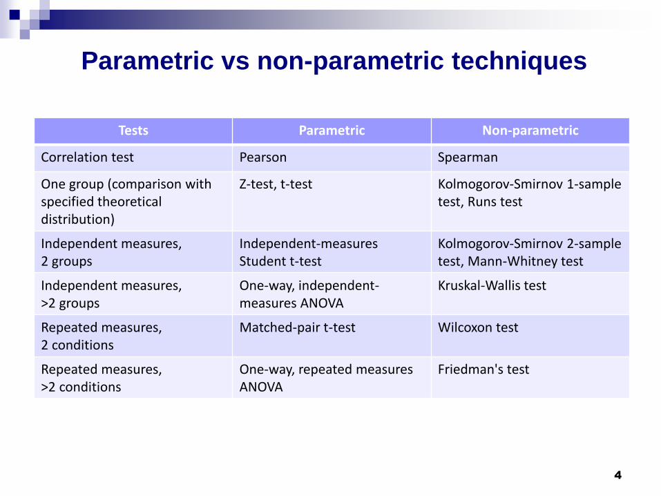
Parametric vs non-parametric techniques
Tests Parametric Non-parametric
Correlation test Pearson Spearman
One group (comparison with specified theoretical distribution)
Z-test, t-test Kolmogorov-Smirnov 1-sampletest, Runs test
Independent measures, 2 groups
Independent-measures Student t-test
Kolmogorov-Smirnov 2-sample test, Mann-Whitney test
Independent measures, >2 groups
One-way, independent-measures ANOVA
Kruskal-Wallis test
Repeated measures, 2 conditions
Matched-pair t-test Wilcoxon test
Repeated measures, >2 conditions
One-way, repeated measures ANOVA
Friedman's test
4
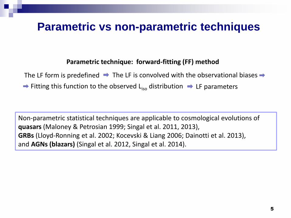
Parametric vs non-parametric techniques
5
Non-parametric statistical techniques are applicable to cosmological evolutions of quasars (Maloney & Petrosian 1999; Singal et al. 2011, 2013), GRBs (Lloyd-Ronning et al. 2002; Kocevski & Liang 2006; Dainotti et al. 2013), and AGNs (blazars) (Singal et al. 2012, Singal et al. 2014).
The LF form is predefined The LF is convolved with the observational biases
Fitting this function to the observed Liso distribution LF parameters
Parametric technique: forward-fitting (FF) method
6
Joint Russian-US Konus-Wind experiment
Two detectors (S1 and S2) are located on opposite faces of spacecraft, observing correspondingly the southern and northern celestial hemispheres;
~100-160 cm2 effective area;
Now around L1 at ~7 light seconds from Earth;
Light curves (LC): ~20 – 1500 keV ;
Waiting mode: LS res. is 2.944 s;
Triggered mode: LC res. is 2 ms –256 ms, from T0-0.512 s to T0+230 s128-ch spectra (20 keV – 20 MeV).
Advantages
Wide energy band: ~20 keV–20 MeV;
Exceptionally stable background;
The orbit of s/c excepts interferences from radiation belts and the Earth shadowing;
Continuous observations of all sky;
Duty circle 95%;
Observes almost all bright events (>10-6erg cm-2 s-1).6
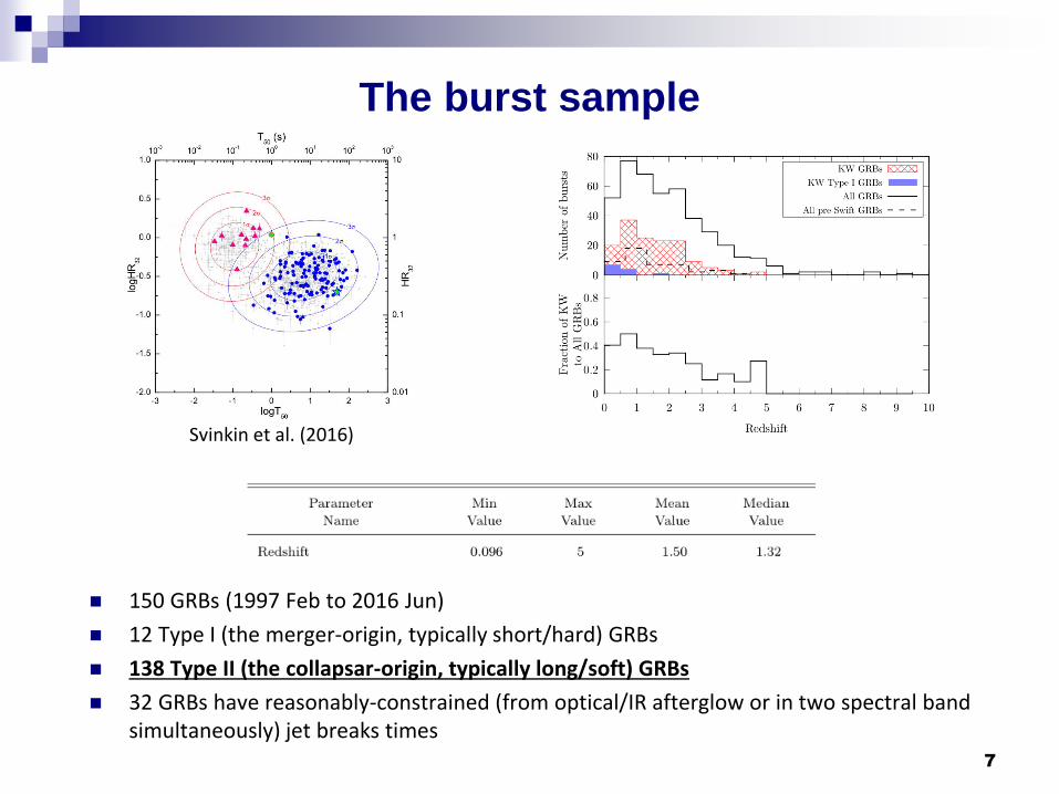
The burst sample
150 GRBs (1997 Feb to 2016 Jun)
12 Type I (the merger-origin, typically short/hard) GRBs
138 Type II (the collapsar-origin, typically long/soft) GRBs
32 GRBs have reasonably-constrained (from optical/IR afterglow or in two spectral band simultaneously) jet breaks times
7
Svinkin et al. (2016)

8
Analysis
The observer-frame energetics range: 10 keV – 10 MeV;
Durations (T100, T90, T50) were calculated in 75 keV – 1 MeV range;
The spectral lags were estimated;
Spectral analysis: time-integrated and peak spectra, CPL and Band models;
Best fit model: χ2CPL-χ
2Band>6 => the Band function;
Based on the GRB redshifts, which span the range 0.1 ≤ z ≤ 5, the rest-frame,
isotropic-equivalent energies (Eiso) and peak luminosities (Liso) were estimated;
Liso were calculated on the (1+z)64 ms time scale, which partially removes the
observational bias;
For 32 GRBs with reasonably-constrained jet breaks the collimation-corrected
values of the energetics are provided.

9
Selection effects
Trigger threshold: 9σ
Solid line: CPL (α= -1)
Dashed line: Band (α= -1, β = -2.5)
Incident angles: 60°
Dependence of the limiting KW energy flux on Ep
Band (2003)
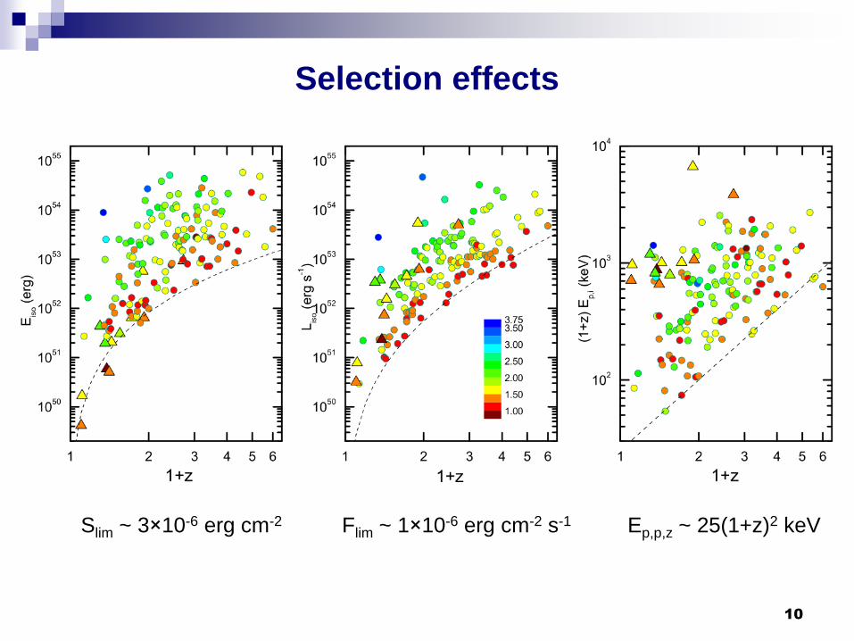
Selection effects
Slim ~ 3×10⁻⁶ erg cm-2
10
Flim ~ 1×10⁻⁶ erg cm-2 s-1 Ep,p,z ~ 25(1+z)2 keV
11
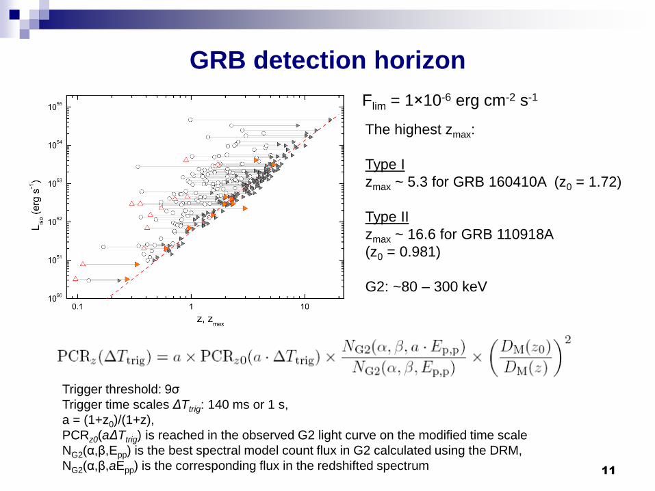
GRB detection horizon
Flim = 1×10⁻⁶ erg cm-2 s-1
Trigger threshold: 9σ
Trigger time scales ΔTtrig: 140 ms or 1 s,
a = (1+z0)/(1+z),
PCRz0(aΔTtrig) is reached in the observed G2 light curve on the modified time scale
NG2(α,β,Epp) is the best spectral model count flux in G2 calculated using the DRM,
NG2(α,β,aEpp) is the corresponding flux in the redshifted spectrum
The highest zmax:
Type I
zmax ~ 5.3 for GRB 160410A (z0 = 1.72)
Type II
zmax ~ 16.6 for GRB 110918A
(z0 = 0.981)
G2: ~80 – 300 keV
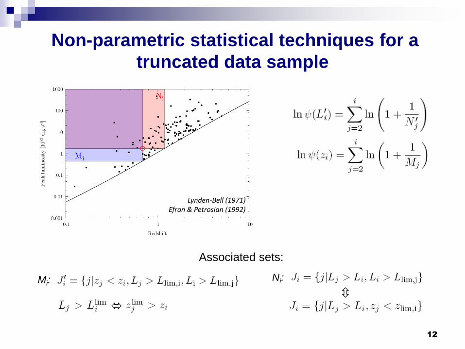
Non-parametric statistical techniques for a
truncated data sample
12
Lynden-Bell (1971)Efron & Petrosian (1992)
Associated sets:
Mi:
Ni:
13
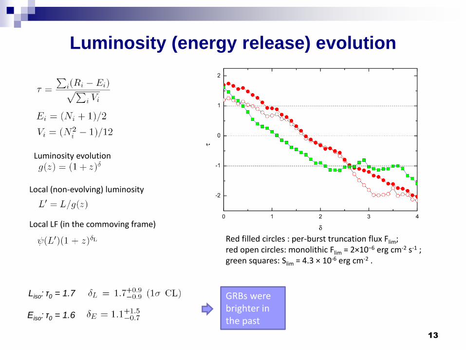
Luminosity (energy release) evolution
Red filled circles : per-burst truncation flux Flim;red open circles: monolithic Flim = 2×10⁻⁶ erg cm-2 s-1 ; green squares: Slim = 4.3 × 10⁻⁶ erg cm-2 .
Liso: τ0 = 1.7
Eiso: τ0 = 1.6
Luminosity evolution
Local LF (in the commoving frame)
Local (non-evolving) luminosity
GRBs were brighter in the past
14
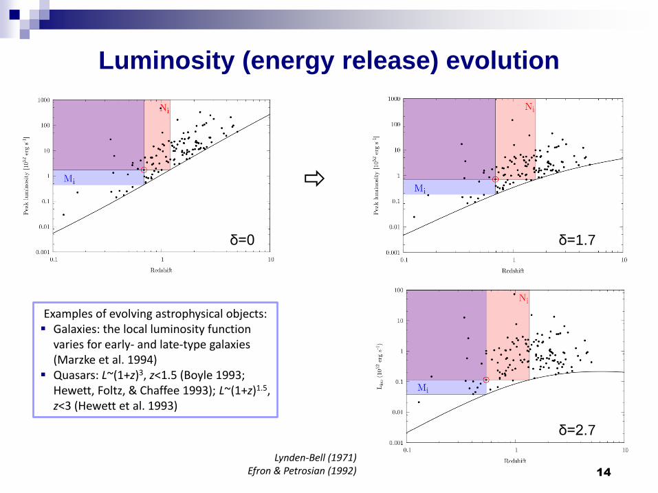
Luminosity (energy release) evolution
Lynden-Bell (1971)Efron & Petrosian (1992)
δ=0 δ=1.7
δ=2.7
Examples of evolving astrophysical objects: Galaxies: the local luminosity function
varies for early- and late-type galaxies (Marzke et al. 1994)
Quasars: L~(1+z)3, z<1.5 (Boyle 1993; Hewett, Foltz, & Chaffee 1993); L~(1+z)1.5, z<3 (Hewett et al. 1993)

15
Selection effects and luminosity (energy
release) evolution
Flim = 2×10⁻⁶ erg cm-2 s-1 ; Slim = 4.3 × 10⁻⁶ erg cm-2 .
Red circles: Luminosity;Green squares: Energy release.
The cosmic background temperature was higher; The metallicity was lower, which implies lower cooling rates and therefore higher temperatures on average; The heating rates were probably higher in the past because the SFR per unit volume was higher, leading to
more intense radiation fields at high redshifts.
16
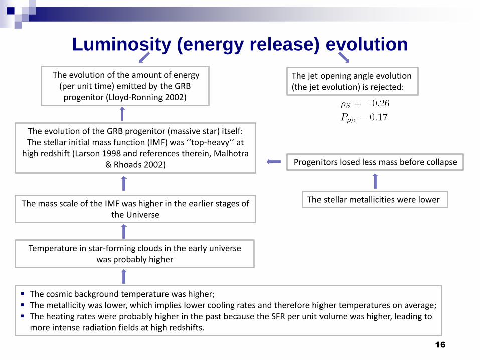
Luminosity (energy release) evolution
The evolution of the amount of energy (per unit time) emitted by the GRB
progenitor (Lloyd-Ronning 2002)
The jet opening angle evolution(the jet evolution) is rejected:
The evolution of the GRB progenitor (massive star) itself:The stellar initial mass function (IMF) was ‘‘top-heavy’’ at
high redshift (Larson 1998 and references therein, Malhotra & Rhoads 2002)
The mass scale of the IMF was higher in the earlier stages of the Universe
Temperature in star-forming clouds in the early universe was probably higher
Progenitors losed less mass before collapse
The stellar metallicities were lower
The present-time GRB luminosity
and energy release functions
17
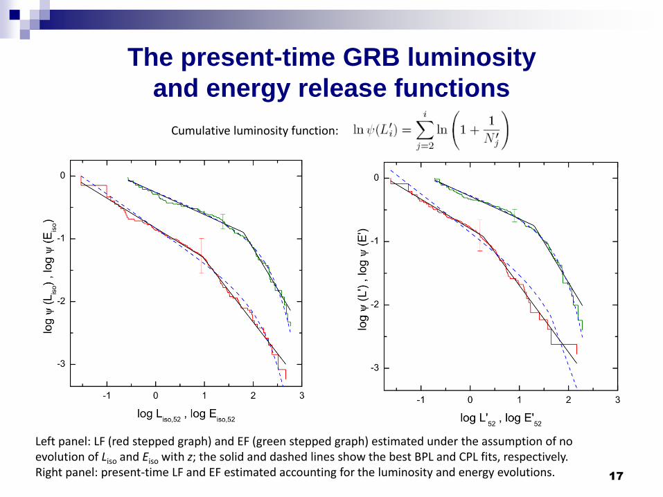
Cumulative luminosity function:
Left panel: LF (red stepped graph) and EF (green stepped graph) estimated under the assumption of no evolution of Liso and Eiso with z; the solid and dashed lines show the best BPL and CPL fits, respectively. Right panel: present-time LF and EF estimated accounting for the luminosity and energy evolutions.

The present-time GRB luminosity
and energy release functions
18
BPL: CPL:
α1, α2 – PL indices at the dim and bright distribution segments,xb – breakpoint of the distribution.
α – PL index,xcut – cutoff luminosity (or energy).

19
GRB formation rate evolution
SFR: Hopkins (2004), Bouwens et al. (2011), Hanish et al. (2006), Thompson et al. (2006), Li (2008).
Red open circles: no luminosity evolution; red filled circles: δL= 1.7;green open squares: no energy evolution; green filled squares: δL = 1.1.
Comoving density rate:
Differential comoving volume:
Hubble distance:
Normalized Hubble parameter:
DM is the transverse comoving distance
Cumulative rate evolution:

20
Summary
A systematic study of 150 GRBs (from 1997 February to 2016 June) with known redshifts was performed;
The influence of instrumental selection effects on the GRB parameter distributions was analyzed: the regions above the limits, corresponding to the bolometric fluence
Slim ∼ 3×10⁻⁶ erg cm-2 (in the Eiso – z plane) and bolometric peak energy flux
Flim ∼ 1×10⁻⁶ erg cm-2 s-1 (in the Liso – z plane) may be considered free from the selection biases;
KW GRB detection horizon extends to zmax ∼ 16.6, stressing the importance of GRBs as probes of the early Universe;
The GRB luminosity evolution, luminosity and energy release functions, and the evolution of the GRB formation rate were estimated accounting for the instrumental bias:
The derived luminosity evolution and isotropic energy evolution indices δL∼1.7 and δE∼1.1 are more shallow than those reported in previous studies, albeit within errors;
The shape of the derived LF is best described by the broken PL function with low- and high-luminosity slopes ∼ −0.5 and ∼ −1, respectively;
The EF is better described by the exponentially-cutoff PL with the PL index ∼ −0.3 and a cutoff isotropic energy of ∼ (2 − 4) × 1054 erg;
The derived GRBFR features an excess over the SFR at z < 1;
GRBs were more luminous in the past than today.

21
Thank you!
Related Documents