1 Non-linear idealisation error analysis of an aerospace stiffened panel loaded in compression Authors: L. Hetey, J. Campbell and R. Vignjevic Crashworthiness, Impact & Structural Mechanics Group, Department of Structures, Impact & Machine Dynamics, Cranfield University, Cranfield, Bedford MK43 0AL, UK Abstract The SAFESA (SAFE Structural Analysis) procedure is an idealisation error control methodology devised for linear static finite element (FE) analysis. This study examines the applicability of this process to non-linear problems. The studied case is the collapse analysis of an aircraft stiffened panel loaded in compression. The paper presents the critical investigation of important modelling assumptions, including the joint modelling, boundary conditions, geometrical imperfections and scattering in material parameters. Potential error sources are identified and then analysed using the non-linear FE solver ABAQUS. The analysis derived an improved FE model and concrete idealisation error estimates. The finally simulated failure behaviour corresponds well to the data measured in the test. Keywords: FEM, Modelling, Error control, Idealisation, ABAQUS, Non-linear 1 Introduction Stiffened panels are essential parts of aerospace structures due to their weight to stiffness ratio. For the safe design of new products it is important to investigate the loading response of these parts and to determine their failure load [1-6]. The outcome is crucial for virtual testing during the certification procedure. Fig. 1: SAFESA in the FE analysis process and involved errors The FE idealisation represents the transformation of a real-world structure into a computer model that can be simulated with the finite element method (FEM), Fig. 1. This process requires making assumptions and simplifications which introduce errors into the final solution. The aim is to establish a rigorous process for identifying these assumptions and controlling the resultant error.

Welcome message from author
This document is posted to help you gain knowledge. Please leave a comment to let me know what you think about it! Share it to your friends and learn new things together.
Transcript
1
Non-linear idealisation error analysis of an aerospace stiffened panel loaded in compression
Authors: L. Hetey, J. Campbell and R. Vignjevic
Crashworthiness, Impact & Structural Mechanics Group, Department of Structures, Impact & Machine Dynamics, Cranfield University, Cranfield, Bedford MK43 0AL, UK
Abstract
The SAFESA (SAFE Structural Analysis) procedure is an idealisation error control methodology devised for linear static finite element (FE) analysis. This study examines the applicability of this process to non-linear problems. The studied case is the collapse analysis of an aircraft stiffened panel loaded in compression. The paper presents the critical investigation of important modelling assumptions, including the joint modelling, boundary conditions, geometrical imperfections and scattering in material parameters. Potential error sources are identified and then analysed using the non-linear FE solver ABAQUS. The analysis derived an improved FE model and concrete idealisation error estimates. The finally simulated failure behaviour corresponds well to the data measured in the test.
Keywords: FEM, Modelling, Error control, Idealisation, ABAQUS, Non-linear
1 Introduction
Stiffened panels are essential parts of aerospace structures due to their weight to stiffness ratio. For the safe design of new products it is important to investigate the loading response of these parts and to determine their failure load [1-6]. The outcome is crucial for virtual testing during the certification procedure.
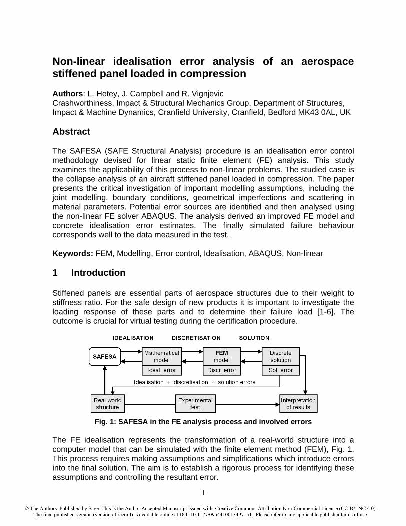
Fig. 1: SAFESA in the FE analysis process and involved errors
The FE idealisation represents the transformation of a real-world structure into a computer model that can be simulated with the finite element method (FEM), Fig. 1. This process requires making assumptions and simplifications which introduce errors into the final solution. The aim is to establish a rigorous process for identifying these assumptions and controlling the resultant error.
e805814
Text Box
Proceedings of the Institution of Mechanical Engineers, Part G: Journal of Aerospace Engineering Volume 228, Issue 9, July 2014, pp. 1574-1585 DOI: 10.1177/0954410013497151
e805814
Text Box
© The Authors. Published by Sage. This is the Author Accepted Manuscript issued with: Creative Commons Attribution Non-Commercial License (CC:BY:NC 4.0). The final published version (version of record) is available online at DOI:10.1177/0954410013497151. Please refer to any applicable publisher terms of use.
2
The idealisation error control process is investigated with the collapse analysis of an aircraft stiffened panel loaded in compression. This is achieved by applying the SAFESA methodology [7,8] which was initially conceived for linear static problems. The goal is to enhance the analysis reliability and to demonstrate that the SAFESA approach can be adapted to non-linear investigations. The text is structured as follows: Section 2 outlines the SAFESA methodology. Section 3 describes the compression panel and the building of a reference FE model. In Section 4 the critical study of possible error sources is discussed. The result is a revised FE model and an assessment of the remaining uncertainty. Section 5 derives conclusions.
2 SAFESA error control procedure SAFESA is an error control procedure for the idealisation of linear static FE analysis [7,8]. In how far the methodology can be extended to more complex problems is in the focus of current research [9,10]. The goal is to provide a methodology which helps analysts in FE modelling. This means that certain error bounds will be obtained, and an identical problem will not lead to widely different results when solved using different codes or by different analysts. Input for the procedure is a real world analysis case (CAD geometry, material properties etc.) and the output is a model ready for meshing. Idealisation decisions are documented with text and need to be confirmed by choosing a confidence level. If the decision cannot be made with certainty they will be flagged and need to be investigated at a following iteration. Idealisation control proceeds step-wise [8,10,11]:
• Step 1: Definition of boundaries, boundary conditions and loading.
• Step 2: Definition of load paths and idealisation of geometry.
• Step 3: Structural segmentation into features and primitives. The feature represents a recognisable entity with coherent properties, while the primitive is part of a feature and is the smallest possible fragmentation. The purpose is to study structural interconnections, and to analyse sub-models that have a manageable complexity.
• Step 4 and 5: Rerun of step one and two at the feature and primitive level.
• Step 6: Review of the conducted analyses up to this point. Either error levels can be derived or experimental testing (Step 7) is required.
• Step 7: Executing corroborative tests. This step can be the most elaborate but provides important modelling data.
Idealisation errors are introduced by the choice of mathematical models, boundary conditions, loading actions, material parameters and the elimination of geometrical details. Experience rules, simplified calculations, hierarchical modelling and sensitivity studies are used to analyse the error. Even if these tools are known to an
3
analyst, it is the consequent application of the procedural steps that improves the model reliability.
3 Reference model building
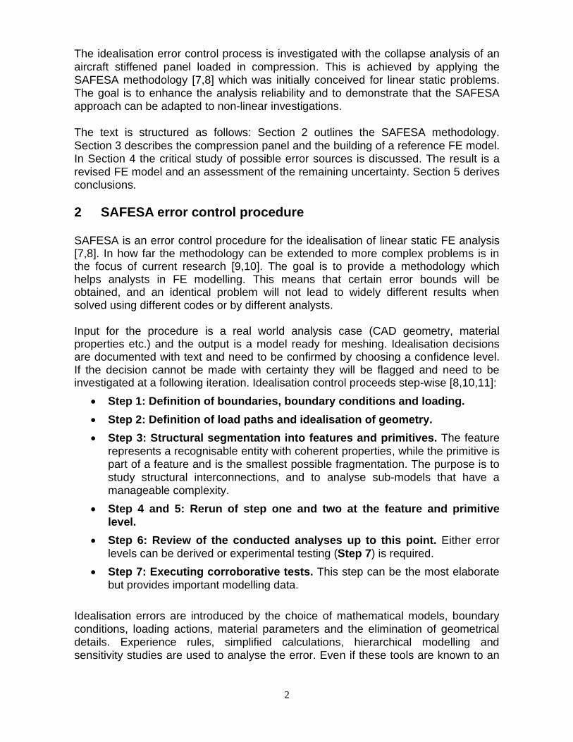
The structure consists of two stiffened panels connected with a buttstrap to form a single unit, Fig. 2-5. The panel length is 1.72 m, and the width is 1.03 m. Fig. 2 shows the CAD model of the panel, which is surrounded by the side frame and end platen.
Fig. 2: CAD model of the panel assembly
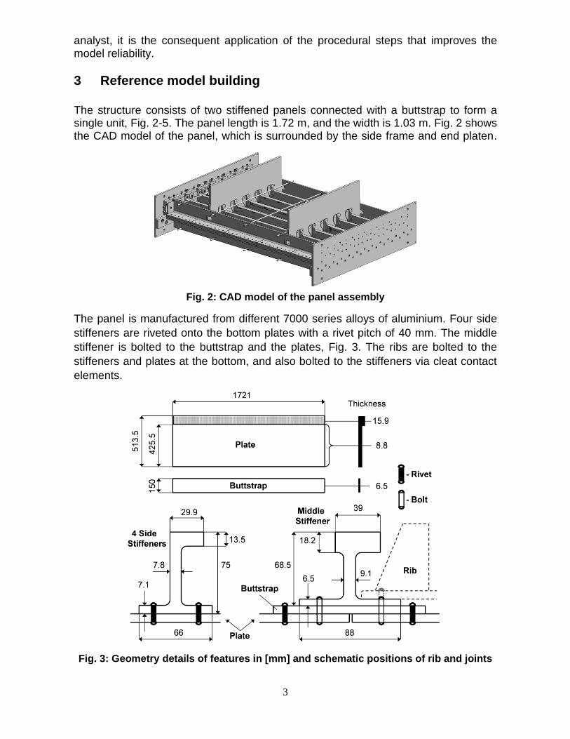
The panel is manufactured from different 7000 series alloys of aluminium. Four side
stiffeners are riveted onto the bottom plates with a rivet pitch of 40 mm. The middle
stiffener is bolted to the buttstrap and the plates, Fig. 3. The ribs are bolted to the
stiffeners and plates at the bottom, and also bolted to the stiffeners via cleat contact
elements.
Fig. 3: Geometry details of features in [mm] and schematic positions of rib and joints
4
Coupon tests for the used joints and aluminium alloys were performed. For the study
of geometrical imperfection, the thickness of plates, buttstrap and the stiffeners were
measured. During the panel test, data was recorded using displacement transducers,
strain gauges, crack detection sensors and speed cameras.
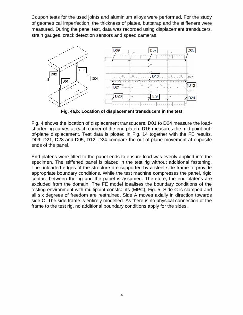
Fig. 4a,b: Location of displacement transducers in the test
Fig. 4 shows the location of displacement transducers. D01 to D04 measure the load-shortening curves at each corner of the end platen. D16 measures the mid point out-of-plane displacement. Test data is plotted in Fig. 14 together with the FE results. D09, D21, D28 and D05, D12, D24 compare the out-of-plane movement at opposite ends of the panel.
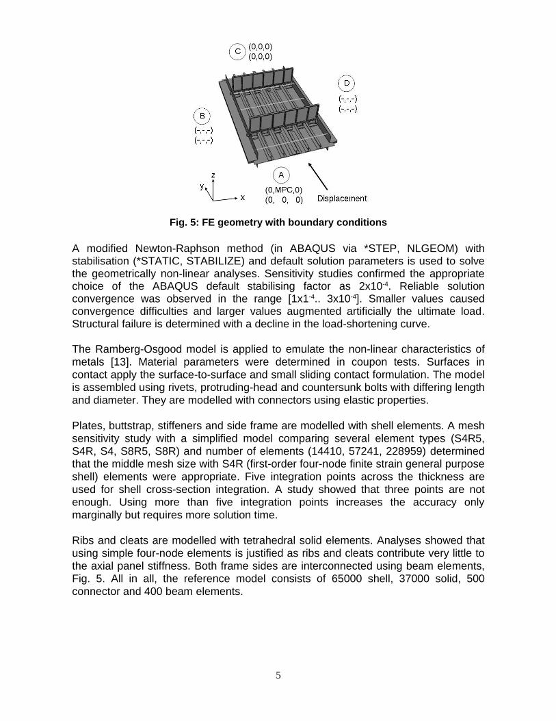
End platens were fitted to the panel ends to ensure load was evenly applied into the specimen. The stiffened panel is placed in the test rig without additional fastening. The unloaded edges of the structure are supported by a steel side frame to provide appropriate boundary conditions. While the test machine compresses the panel, rigid contact between the rig and the panel is assumed. Therefore, the end platens are excluded from the domain. The FE model idealises the boundary conditions of the testing environment with multipoint constraints (MPC), Fig. 5. Side C is clamped and all six degrees of freedom are restrained. Side A moves axially in direction towards side C. The side frame is entirely modelled. As there is no physical connection of the frame to the test rig, no additional boundary conditions apply for the sides.
5
Fig. 5: FE geometry with boundary conditions
A modified Newton-Raphson method (in ABAQUS via *STEP, NLGEOM) with stabilisation (*STATIC, STABILIZE) and default solution parameters is used to solve the geometrically non-linear analyses. Sensitivity studies confirmed the appropriate choice of the ABAQUS default stabilising factor as 2x10⁻⁴. Reliable solution convergence was observed in the range [1x1-4.. 3x10⁻⁴]. Smaller values caused convergence difficulties and larger values augmented artificially the ultimate load. Structural failure is determined with a decline in the load-shortening curve. The Ramberg-Osgood model is applied to emulate the non-linear characteristics of metals [13]. Material parameters were determined in coupon tests. Surfaces in contact apply the surface-to-surface and small sliding contact formulation. The model is assembled using rivets, protruding-head and countersunk bolts with differing length and diameter. They are modelled with connectors using elastic properties. Plates, buttstrap, stiffeners and side frame are modelled with shell elements. A mesh sensitivity study with a simplified model comparing several element types (S4R5, S4R, S4, S8R5, S8R) and number of elements (14410, 57241, 228959) determined that the middle mesh size with S4R (first-order four-node finite strain general purpose shell) elements were appropriate. Five integration points across the thickness are
used for shell cross-section integration. A study showed that three points are not enough. Using more than five integration points increases the accuracy only marginally but requires more solution time. Ribs and cleats are modelled with tetrahedral solid elements. Analyses showed that using simple four-node elements is justified as ribs and cleats contribute very little to the axial panel stiffness. Both frame sides are interconnected using beam elements, Fig. 5. All in all, the reference model consists of 65000 shell, 37000 solid, 500 connector and 400 beam elements.
6
4 Idealisation error investigation using SAFESA The execution of the error control procedure determined the following idealisation uncertainties [10]:
• sensitivity to boundary conditions,
• check if load path changes when nonlinear-behaviour starts,
• joint modelling,
• joints connecting several material layers,
• stiffener modelling with shell or solid elements,
• influence of stiffener mid-surfaces,
• plate and side frame contact,
• geometrical imperfections, and
• scattering in material parameters. The FE modelling was corrected iteratively, and the comparison between idealisations is based on the relative impact within each error source. The remaining uncertainty is the change in failure load of the reference model when modifying the idealisation. The resulting error levels were rounded to per cent values.
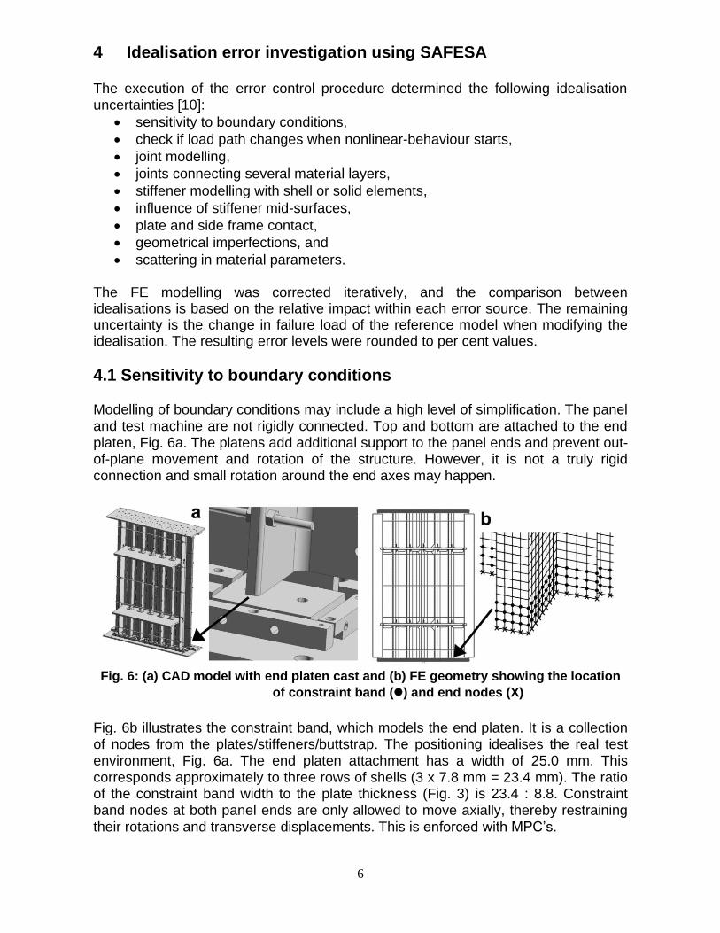
4.1 Sensitivity to boundary conditions Modelling of boundary conditions may include a high level of simplification. The panel and test machine are not rigidly connected. Top and bottom are attached to the end platen, Fig. 6a. The platens add additional support to the panel ends and prevent out-of-plane movement and rotation of the structure. However, it is not a truly rigid connection and small rotation around the end axes may happen.
Fig. 6: (a) CAD model with end platen cast and (b) FE geometry showing the location
of constraint band (⚫) and end nodes (X)
Fig. 6b illustrates the constraint band, which models the end platen. It is a collection of nodes from the plates/stiffeners/buttstrap. The positioning idealises the real test environment, Fig. 6a. The end platen attachment has a width of 25.0 mm. This corresponds approximately to three rows of shells (3 x 7.8 mm = 23.4 mm). The ratio of the constraint band width to the plate thickness (Fig. 3) is 23.4 : 8.8. Constraint band nodes at both panel ends are only allowed to move axially, thereby restraining their rotations and transverse displacements. This is enforced with MPC’s.
7
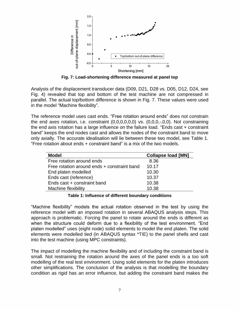
Fig. 7: Load-shortening difference measured at panel top
Analysis of the displacement transducer data (D09, D21, D28 vs. D05, D12, D24, see Fig. 4) revealed that top and bottom of the test machine are not compressed in parallel. The actual top/bottom difference is shown in Fig. 7. These values were used in the model “Machine flexibility”. The reference model uses cast ends. “Free rotation around ends” does not constrain the end axes rotation, i.e. constraint (0,0,0,0,0,0) vs. (0,0,0,-,0,0). Not constraining the end axis rotation has a large influence on the failure load. “Ends cast + constraint band” keeps the end nodes cast and allows the nodes of the constraint band to move only axially. The accurate idealisation will lie between these two model, see Table 1. “Free rotation about ends + constraint band” is a mix of the two models.
Model Collapse load [MN]
Free rotation around ends 8.36 Free rotation around ends + constraint band 10.17 End platen modelled 10.30 Ends cast (reference) 10.37 Ends cast + constraint band 10.38 Machine flexibility 10.38
Table 1: Influence of different boundary conditions
“Machine flexibility” models the actual rotation observed in the test by using the reference model with an imposed rotation in several ABAQUS analysis steps. This approach is problematic. Forcing the panel to rotate around the ends is different as when the structure could deform due to a flexibility of the test environment. “End platen modelled” uses (eight node) solid elements to model the end platen. The solid elements were modelled tied (in ABAQUS syntax *TIE) to the panel shells and cast into the test machine (using MPC constraints).
The impact of modelling the machine flexibility and of including the constraint band is small. Not restraining the rotation around the axes of the panel ends is a too soft modelling of the real test environment. Using solid elements for the platen introduces other simplifications. The conclusion of the analysis is that modelling the boundary condition as rigid has an error influence, but adding the constraint band makes the
8
model more realistic. An idealisation error of 2% (“Reference” vs. “Constraint band + free rotation around ends”) results due to the remaining end platen flexibility.
4.2 Check if the load path changes when non-linear behaviour starts This investigation addresses geometrical nonlinearity. Different stages in the loading process were anticipated in the idealisation phase:
• Linear elastic material deformation at lower stress levels.
• No local buckling. Thin-walled stiffened panels start buckling locally in the skin between stiffeners when compressed axially. But the panel in this study is a thick one, and no local buckling of the skin plate occurs.
• Global bending of the whole structure. At this point the stringers start buckling and the load path will change.
• Failure of a joint connection. This local failure will most likely be followed by a global collapse of the panel.
• Collapse of the structure. The structure deforms plastically and the capability to carry load is decreased.
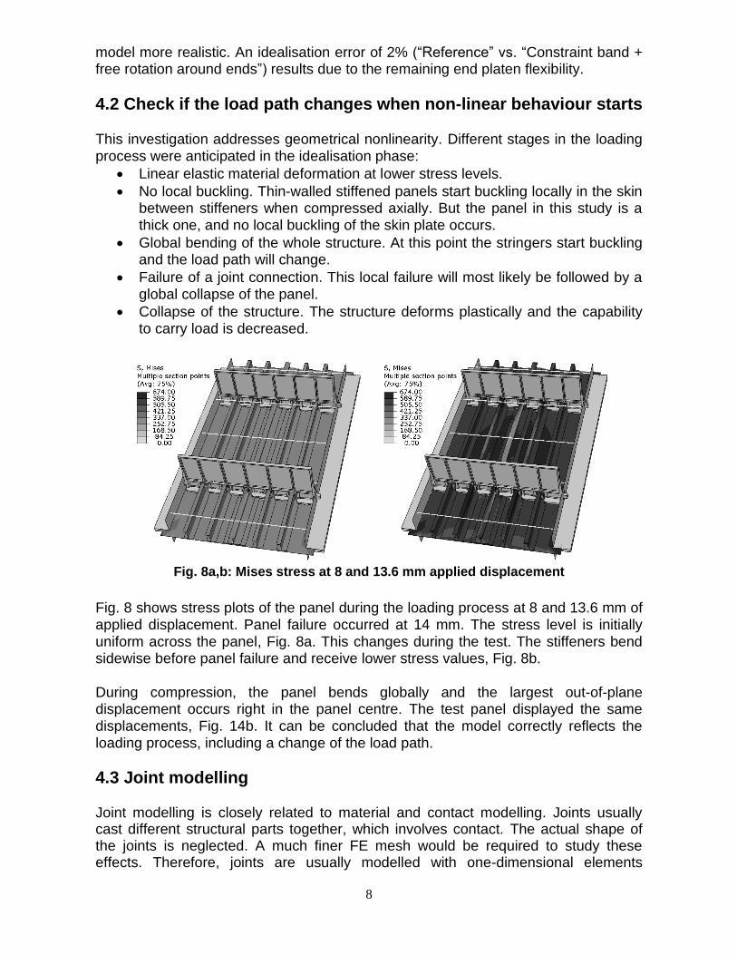
Fig. 8a,b: Mises stress at 8 and 13.6 mm applied displacement
Fig. 8 shows stress plots of the panel during the loading process at 8 and 13.6 mm of applied displacement. Panel failure occurred at 14 mm. The stress level is initially
uniform across the panel, Fig. 8a. This changes during the test. The stiffeners bend sidewise before panel failure and receive lower stress values, Fig. 8b. During compression, the panel bends globally and the largest out-of-plane displacement occurs right in the panel centre. The test panel displayed the same displacements, Fig. 14b. It can be concluded that the model correctly reflects the loading process, including a change of the load path.
4.3 Joint modelling Joint modelling is closely related to material and contact modelling. Joints usually cast different structural parts together, which involves contact. The actual shape of the joints is neglected. A much finer FE mesh would be required to study these effects. Therefore, joints are usually modelled with one-dimensional elements
9
between two nodes. Common joint models use springs, beams and connectors. ABAQUS offers several options for connector elements [12]:
• Connector_beam constrains the translation and rotation of the first node to the translation and rotation at the second node.
• Connector_link enforces a constant distance between two nodes, but allows rotations.
• Connector_cartesian connects two nodes using specific properties. Elasticity, plasticity, friction, damage or failure can be specified independently in three local Cartesian directions.
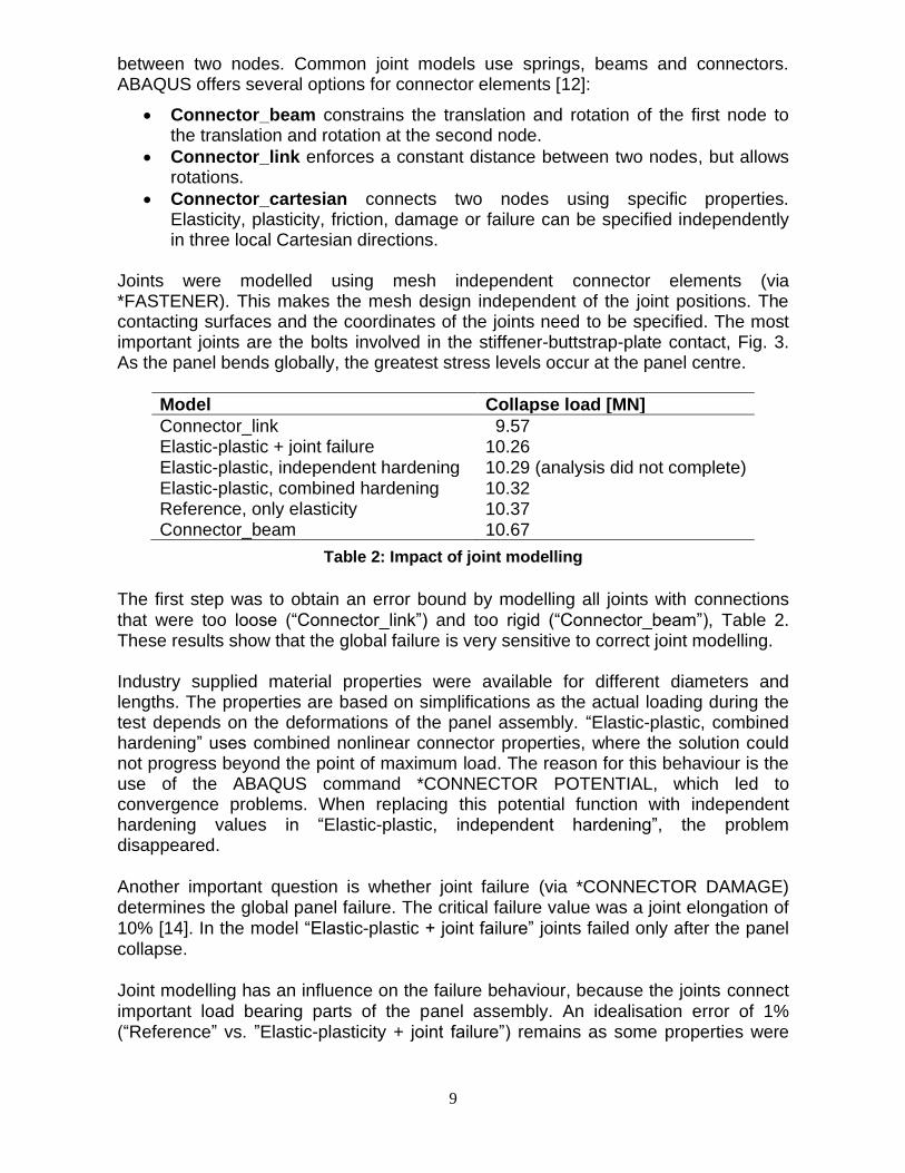
Joints were modelled using mesh independent connector elements (via *FASTENER). This makes the mesh design independent of the joint positions. The contacting surfaces and the coordinates of the joints need to be specified. The most important joints are the bolts involved in the stiffener-buttstrap-plate contact, Fig. 3. As the panel bends globally, the greatest stress levels occur at the panel centre.
Model Collapse load [MN]
Connector_link 9.57 Elastic-plastic + joint failure 10.26 Elastic-plastic, independent hardening 10.29 (analysis did not complete) Elastic-plastic, combined hardening 10.32 Reference, only elasticity 10.37 Connector_beam 10.67
Table 2: Impact of joint modelling
The first step was to obtain an error bound by modelling all joints with connections that were too loose (“Connector_link”) and too rigid (“Connector_beam”), Table 2. These results show that the global failure is very sensitive to correct joint modelling. Industry supplied material properties were available for different diameters and lengths. The properties are based on simplifications as the actual loading during the test depends on the deformations of the panel assembly. “Elastic-plastic, combined hardening” uses combined nonlinear connector properties, where the solution could not progress beyond the point of maximum load. The reason for this behaviour is the use of the ABAQUS command *CONNECTOR POTENTIAL, which led to convergence problems. When replacing this potential function with independent hardening values in “Elastic-plastic, independent hardening”, the problem disappeared. Another important question is whether joint failure (via *CONNECTOR DAMAGE) determines the global panel failure. The critical failure value was a joint elongation of 10% [14]. In the model “Elastic-plastic + joint failure” joints failed only after the panel collapse. Joint modelling has an influence on the failure behaviour, because the joints connect important load bearing parts of the panel assembly. An idealisation error of 1% (“Reference” vs. ”Elastic-plasticity + joint failure”) remains as some properties were
10
determined using engineering assumptions. The final model will incorporate the elastic-plastic joint properties with independent hardening.
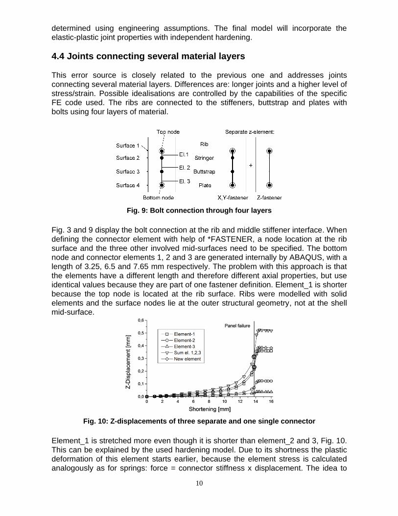
4.4 Joints connecting several material layers This error source is closely related to the previous one and addresses joints connecting several material layers. Differences are: longer joints and a higher level of stress/strain. Possible idealisations are controlled by the capabilities of the specific FE code used. The ribs are connected to the stiffeners, buttstrap and plates with bolts using four layers of material.
Fig. 9: Bolt connection through four layers
Fig. 3 and 9 display the bolt connection at the rib and middle stiffener interface. When defining the connector element with help of *FASTENER, a node location at the rib surface and the three other involved mid-surfaces need to be specified. The bottom node and connector elements 1, 2 and 3 are generated internally by ABAQUS, with a length of 3.25, 6.5 and 7.65 mm respectively. The problem with this approach is that the elements have a different length and therefore different axial properties, but use identical values because they are part of one fastener definition. Element_1 is shorter because the top node is located at the rib surface. Ribs were modelled with solid elements and the surface nodes lie at the outer structural geometry, not at the shell mid-surface.
Fig. 10: Z-displacements of three separate and one single connector
Element_1 is stretched more even though it is shorter than element_2 and 3, Fig. 10. This can be explained by the used hardening model. Due to its shortness the plastic deformation of this element starts earlier, because the element stress is calculated analogously as for springs: force = connector stiffness x displacement. The idea to
11
model these joints in a more realistic way is to move the z-component definition into a separate element, as illustrated in the right side of Fig. 9. Now, this connector will deform uniformly, leading to a more realistic model. The impact of this approach is shown in Fig. 10. The “New element” deforms less than the sum of the three separate elements. The element deformation at panel failure decreases from 0.32 to 0.23 mm, as indicated. This error source did not show much influence on the global failure behaviour as these bolts are located far from the panel centre. For analyses where mesh independent fasteners using several material layers are located in more critical regions it can become important. Nevertheless, the updated model will include this improvement.
4.5 Stiffener modelling with shell or solid elements Panel plates, buttstrap and stiffeners are plane, and will be modelled using general purpose shell elements. Classical shell theory is applicable, i.e. the length-thickness ratio is large (Fig. 3):
• panel plates (l/t = 425.5/8.8 = 48.35), and
• buttsrap (l/t = 150/6.5 = 23.08). Critical are the cross sections of the stiffeners’ top:
• side stiffeners (l/t = 29.9/13.5 = 2.21), and
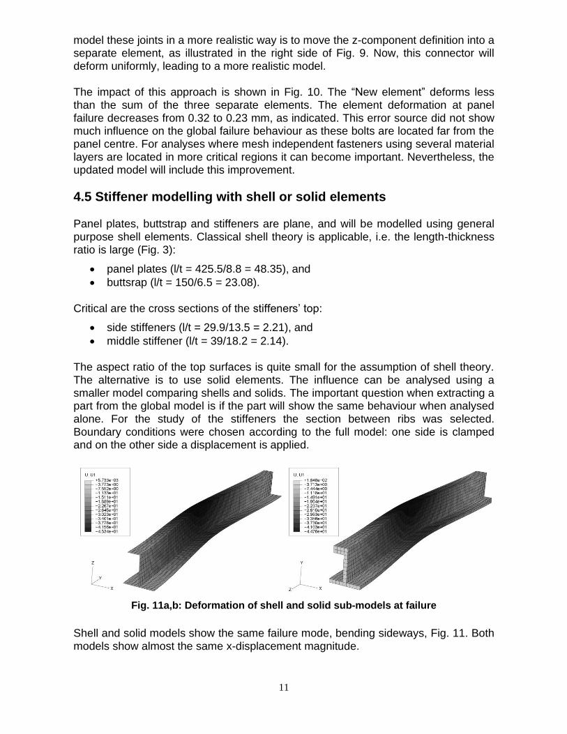
• middle stiffener (l/t = 39/18.2 = 2.14). The aspect ratio of the top surfaces is quite small for the assumption of shell theory. The alternative is to use solid elements. The influence can be analysed using a smaller model comparing shells and solids. The important question when extracting a part from the global model is if the part will show the same behaviour when analysed alone. For the study of the stiffeners the section between ribs was selected. Boundary conditions were chosen according to the full model: one side is clamped and on the other side a displacement is applied.
Fig. 11a,b: Deformation of shell and solid sub-models at failure
Shell and solid models show the same failure mode, bending sideways, Fig. 11. Both models show almost the same x-displacement magnitude.
12
Model S4R [kN] S4 [kN] No. el. C3D8I [kN] C3D20 [kN] No. el.
Coarse 774.63 786.18 1960 782.73 791.18 2352 Middle 775.72 781.23 7840 784.87 786.12 18816 Fine 775.71 776.80 31360 783.66 783.25 150528
Table 3: Collapse load of stiffeners modelled with shell or solid elements
Table 3 summarises the outcome of this analysis. Three mesh sizes were used, each time halving the length of each element side. Shells were divided into four quadratic and solids into eight cubic elements. The “Fine” solid model provides therefore four solid elements across the wall thickness. The stiffener failure load, which was measured as a drop in reaction force, is the interesting criterion. First order C3D8I and second order C3D20 solid elements were compared with S4 and S4R shells. The shell models converged to a failure load of 776 kN and the solid models to a
value of 783 kN, which is less than 1% difference. The error introduced by using shell elements on the full model can be considered as minor. Shells have the great advantage of being more economic in computing.
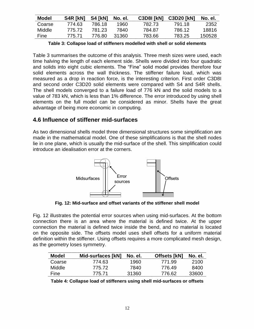
4.6 Influence of stiffener mid-surfaces As two dimensional shells model three dimensional structures some simplification are made in the mathematical model. One of these simplifications is that the shell nodes lie in one plane, which is usually the mid-surface of the shell. This simplification could introduce an idealisation error at the corners.
Fig. 12: Mid-surface and offset variants of the stiffener shell model
Fig. 12 illustrates the potential error sources when using mid-surfaces. At the bottom connection there is an area where the material is defined twice. At the upper connection the material is defined twice inside the bend, and no material is located on the opposite side. The offsets model uses shell offsets for a uniform material definition within the stiffener. Using offsets requires a more complicated mesh design, as the geometry loses symmetry.
Model Mid-surfaces [kN] No. el. Offsets [kN] No. el.
Coarse 774.63 1960 771.99 2100 Middle 775.72 7840 776.49 8400 Fine 775.71 31360 776.62 33600
Table 4: Collapse load of stiffeners using shell mid-surfaces or offsets
13
Table 4 compares the results of these models. “Mid-surfaces” are the same “S4R” models as in the previous section. The difference in ultimate load is not important and no idealisation error is concluded from using mid-surfaces.
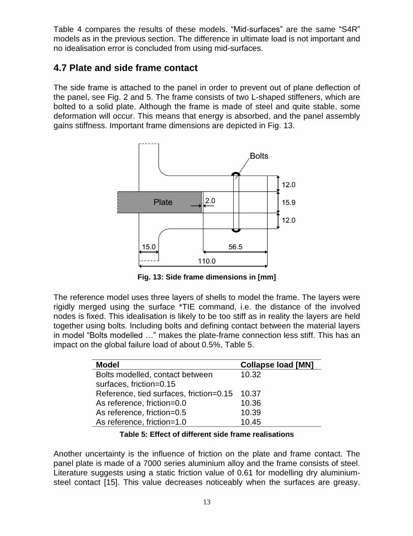
4.7 Plate and side frame contact The side frame is attached to the panel in order to prevent out of plane deflection of the panel, see Fig. 2 and 5. The frame consists of two L-shaped stiffeners, which are bolted to a solid plate. Although the frame is made of steel and quite stable, some deformation will occur. This means that energy is absorbed, and the panel assembly gains stiffness. Important frame dimensions are depicted in Fig. 13.
Fig. 13: Side frame dimensions in [mm]
The reference model uses three layers of shells to model the frame. The layers were rigidly merged using the surface *TIE command, i.e. the distance of the involved nodes is fixed. This idealisation is likely to be too stiff as in reality the layers are held together using bolts. Including bolts and defining contact between the material layers in model “Bolts modelled …” makes the plate-frame connection less stiff. This has an impact on the global failure load of about 0.5%, Table 5.
Model Collapse load [MN]
Bolts modelled, contact between surfaces, friction=0.15
10.32
Reference, tied surfaces, friction=0.15 10.37 As reference, friction=0.0 10.36 As reference, friction=0.5 10.39 As reference, friction=1.0 10.45
Table 5: Effect of different side frame realisations
Another uncertainty is the influence of friction on the plate and frame contact. The panel plate is made of a 7000 series aluminium alloy and the frame consists of steel. Literature suggests using a static friction value of 0.61 for modelling dry aluminium-steel contact [15]. This value decreases noticeably when the surfaces are greasy.
14
The contact is initially loose and gets tightened when the panel deforms. As the frame is attached to the panel, only slight mutual movement occurs. It can be concluded that including bolts improves the model reliability. The friction value of 0.15 was determined by the project partner and will be maintained.
4.8 Geometrical imperfections The FE model assumes perfectly even surfaces and all dimensions without local variations. The real panel geometry deviates from this perfect structure. The thickness of plates, buttstrap and stiffeners was measured along their length with a resolution of 1 µm. The measured thickness was usually bigger than specified in the CAD model, but not evenly distributed. The average difference was around 0.5% of the panel thickness, and the peak difference had a magnitude of 0.8%.
Three options of imperfection modelling will be compared for this investigation:
• creating a new mesh including the imperfection,
• adding eigenmode shapes, and
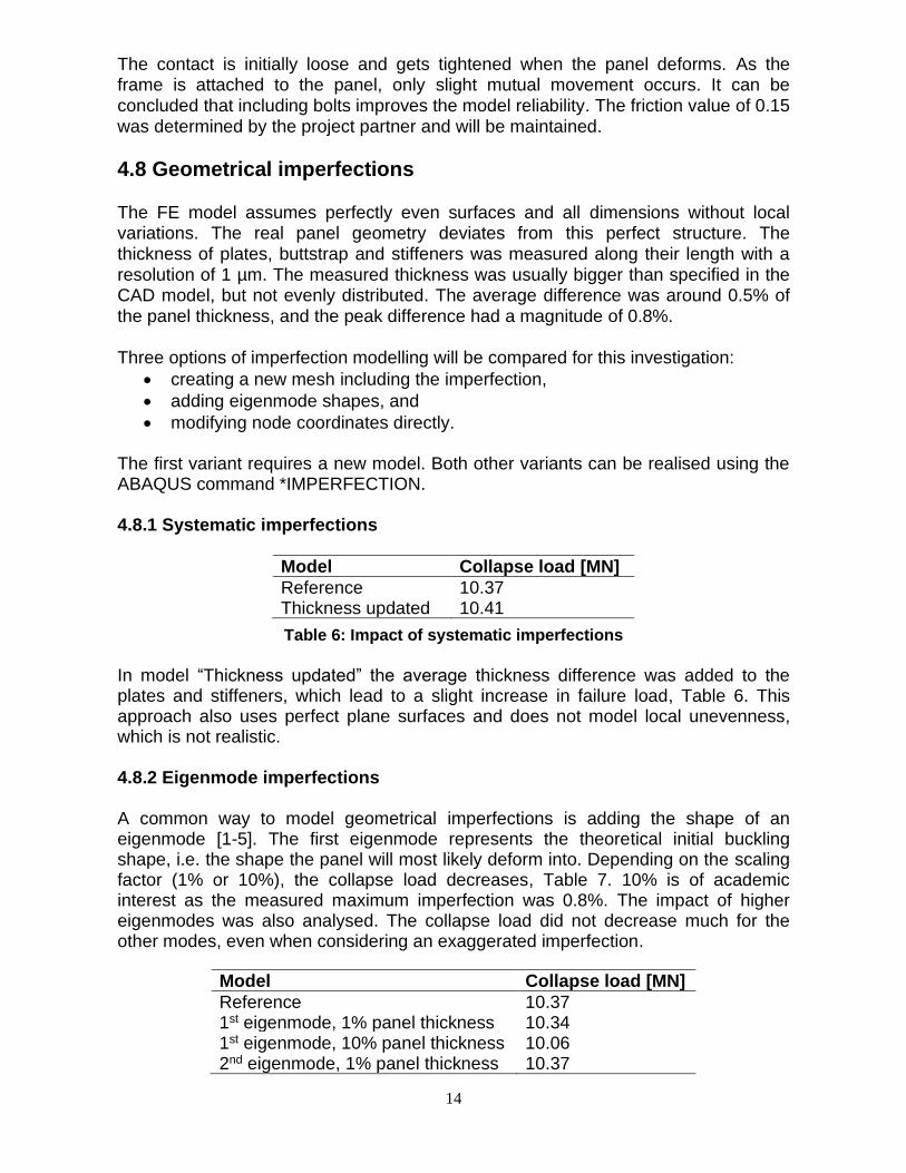
• modifying node coordinates directly. The first variant requires a new model. Both other variants can be realised using the ABAQUS command *IMPERFECTION. 4.8.1 Systematic imperfections
Model Collapse load [MN]
Reference 10.37 Thickness updated 10.41
Table 6: Impact of systematic imperfections
In model “Thickness updated” the average thickness difference was added to the plates and stiffeners, which lead to a slight increase in failure load, Table 6. This approach also uses perfect plane surfaces and does not model local unevenness, which is not realistic. 4.8.2 Eigenmode imperfections A common way to model geometrical imperfections is adding the shape of an eigenmode [1-5]. The first eigenmode represents the theoretical initial buckling shape, i.e. the shape the panel will most likely deform into. Depending on the scaling factor (1% or 10%), the collapse load decreases, Table 7. 10% is of academic interest as the measured maximum imperfection was 0.8%. The impact of higher eigenmodes was also analysed. The collapse load did not decrease much for the other modes, even when considering an exaggerated imperfection.
Model Collapse load [MN]
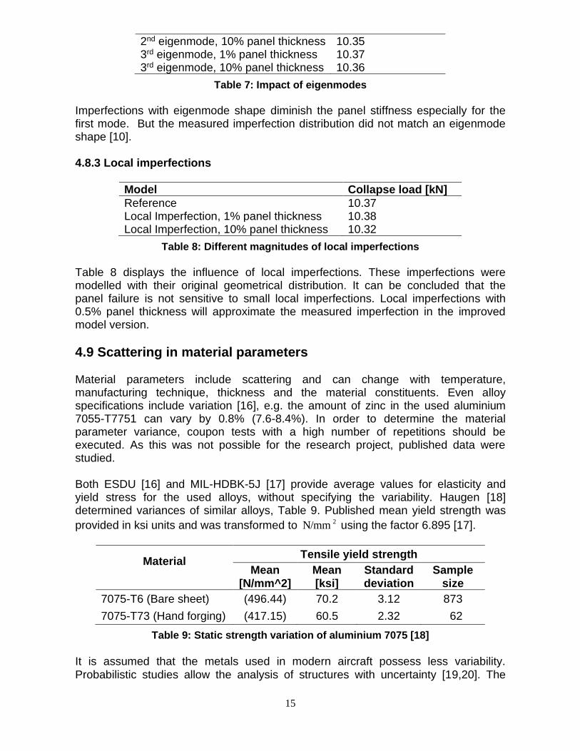
Reference 10.37 1st eigenmode, 1% panel thickness 10.34 1st eigenmode, 10% panel thickness 10.06 2nd eigenmode, 1% panel thickness 10.37
15
2nd eigenmode, 10% panel thickness 10.35 3rd eigenmode, 1% panel thickness 10.37 3rd eigenmode, 10% panel thickness 10.36
Table 7: Impact of eigenmodes
Imperfections with eigenmode shape diminish the panel stiffness especially for the first mode. But the measured imperfection distribution did not match an eigenmode shape [10]. 4.8.3 Local imperfections
Model Collapse load [kN]
Reference 10.37 Local Imperfection, 1% panel thickness 10.38 Local Imperfection, 10% panel thickness 10.32
Table 8: Different magnitudes of local imperfections
Table 8 displays the influence of local imperfections. These imperfections were modelled with their original geometrical distribution. It can be concluded that the panel failure is not sensitive to small local imperfections. Local imperfections with 0.5% panel thickness will approximate the measured imperfection in the improved model version.
4.9 Scattering in material parameters Material parameters include scattering and can change with temperature, manufacturing technique, thickness and the material constituents. Even alloy specifications include variation [16], e.g. the amount of zinc in the used aluminium 7055-T7751 can vary by 0.8% (7.6-8.4%). In order to determine the material parameter variance, coupon tests with a high number of repetitions should be executed. As this was not possible for the research project, published data were studied. Both ESDU [16] and MIL-HDBK-5J [17] provide average values for elasticity and yield stress for the used alloys, without specifying the variability. Haugen [18] determined variances of similar alloys, Table 9. Published mean yield strength was
provided in ksi units and was transformed to 2N/mm using the factor 6.895 [17].
Material
Tensile yield strength
Mean [N/mm^2]
Mean [ksi]
Standard deviation
Sample size
7075-T6 (Bare sheet) (496.44) 70.2 3.12 873
7075-T73 (Hand forging) (417.15) 60.5 2.32 62
Table 9: Static strength variation of aluminium 7075 [18]
It is assumed that the metals used in modern aircraft possess less variability. Probabilistic studies allow the analysis of structures with uncertainty [19,20]. The
16
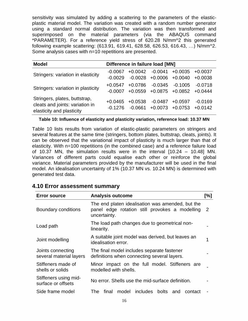
sensitivity was simulated by adding a scattering to the parameters of the elastic-plastic material model. The variation was created with a random number generator using a standard normal distribution. The variation was then transformed and superimposed on the material parameters (via the ABAQUS command *PARAMETER). For a reference yield stress of 620.28 N/mm^2 this generated following example scattering: (613.91, 619.41, 628.58, 626.53, 616.43, …) N/mm^2. Some analysis cases with n=10 repetitions are presented.
Model Difference in failure load [MN]
Stringers: variation in elasticity -0.0067
-0.0029
+0.0042
-0.0028
-0.0041
+0.0006
+0.0035
+0.0040
+0.0037
+0.0038
Stringers: variation in plasticity +0.0547
-0.0007
+0.0786
+0.0559
-0.0345
+0.0875
-0.1005
+0.0852
-0.0718
+0.0444
Stringers, plates, buttstrap,
cleats and joints: variation in
elasticity and plasticity
+0.0465
-0.1276
+0.0538
-0.0661
-0.0487
+0.0073
+0.0597
+0.0753
-0.0169
+0.0142
Table 10: Influence of elasticity and plasticity variation, reference load: 10.37 MN
Table 10 lists results from variation of elastic-plastic parameters on stringers and several features at the same time (stringers, bottom plates, buttstrap, cleats, joints). It can be observed that the variational impact of plasticity is much larger than that of elasticity. With n=100 repetitions (in the combined case) and a reference failure load of 10.37 MN, the simulation results were in the interval [10.24 – 10.48] MN. Variances of different parts could equalise each other or reinforce the global variance. Material parameters provided by the manufacturer will be used in the final model. An idealisation uncertainty of 1% (10.37 MN vs. 10.24 MN) is determined with generated test data.
4.10 Error assessment summary
Error source Analysis outcome [%]
Boundary conditions The end platen idealisation was amended, but the panel edge rotation still provokes a modelling uncertainty.
2
Load path The load path changes due to geometrical non-linearity.
-
Joint modelling A suitable joint model was derived, but leaves an idealisation error.
1
Joints connecting several material layers
The final model includes separate fastener definitions when connecting several layers.
-
Stiffeners made of shells or solids
Minor impact on the full model. Stiffeners are modelled with shells.
-
Stiffeners using mid-surface or offsets
No error. Shells use the mid-surface definition. -
Side frame model The final model includes bolts and contact -
17
between frame layers. The sliding panel-frame contact uses friction.
Geometrical imperfection
The final model contains local imperfections. -
Scattering in material parameter
Published material parameter variances were used to simulate the modelling impact.
1
Table 11: Error assessment summary
Table 11 provides a summary of the idealisation errors. The remaining idealisation uncertainty is indicated in the column entitled “[%]“. The error sources can be interdependent in reality. The interaction is problem specific and difficult to quantify. Applying the error control procedure allowed the identification and quantitative determination of idealisation errors. The results may be used to define a conservative lowest failure load.
4.11 Final model The improved model is updated based on the conclusions from the studies of each individual error source. The result is a model where the level of error introduced by the idealisation process is known and limited at a level acceptable to the analyst.
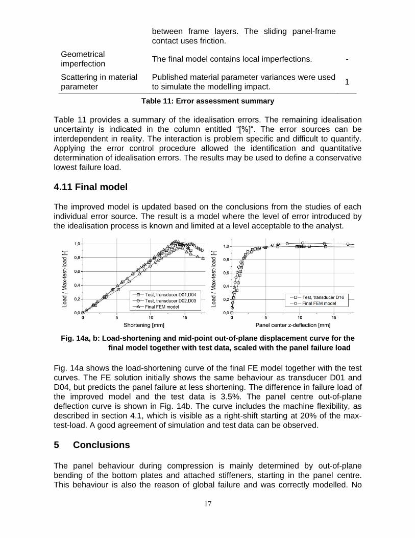
Fig. 14a, b: Load-shortening and mid-point out-of-plane displacement curve for the
final model together with test data, scaled with the panel failure load
Fig. 14a shows the load-shortening curve of the final FE model together with the test curves. The FE solution initially shows the same behaviour as transducer D01 and D04, but predicts the panel failure at less shortening. The difference in failure load of the improved model and the test data is 3.5%. The panel centre out-of-plane deflection curve is shown in Fig. 14b. The curve includes the machine flexibility, as described in section 4.1, which is visible as a right-shift starting at 20% of the max-test-load. A good agreement of simulation and test data can be observed.
5 Conclusions The panel behaviour during compression is mainly determined by out-of-plane bending of the bottom plates and attached stiffeners, starting in the panel centre. This behaviour is also the reason of global failure and was correctly modelled. No
18
local skin buckling takes place because the panel is thick-walled. This also explains the small impact of geometrical imperfections and the problems with the joints connecting several material layers. The improved model includes an idealisation uncertainty which is caused by the boundary conditions, joint modelling and material property variation. Applying SAFESA for the non-linear analysis case improves the FE idealisation outcome and determines concrete error bounds. The final FE failure load is 3.5% higher than in the test, which is a reliable prediction.
Acknowledgements
The work presented in this paper has been financially supported by the project MUSCA (acronym for "non-linear static MUltiSCAle analysis of large aero-structures"), partially funded by the European Union under the Sixth Framework Programme (Project Reference 516115). The authors would like to thank Prof. Dr. A. Morris, J.C. Brown, D. Schumann and the reviewers for their advice and the project partners for supplying the panel data and their valuable feedback.
References [1] Heitmann, M., Horst, P., and Fitzsimmons, D. Effective stiffness of postbuckled stiffened metallic panels under combined compression and shear stress. J. Strain Anal. Eng. Des., 2003, 38(6), 539-555. [2] Lynch, C., Murphy, A., Price, M., and Gibson, A. The computational analysis of fuselage stiffened panels loaded in compression. Thin-Walled Struct., 2004, 42(10), 1445-1464. [3] Murphy, A., Price, M., Gibson, A., and Armstrong, C. G. Efficient non-linear idealisations of aircraft fuselage panels in compression. Finite Elem. Anal. Des., 2004, 40(13-14), 1978-1993. [4] Hughes, O. F., Ghosh, B., and Chen, Y. Improved prediction of simultaneous local and overall buckling of stiffened panels. Thin-Walled Struct., 2004, 42(6), 827-856. [5] Sadovský, Z., Ďuricová, A., Ivančo, V., and Kriváček, J. Imperfection measures of eigen- and periodic modes of axially loaded stringer-stiffened cylindrical shells. Proc IMechE, Part G: J. of Aerospace Engineering, 2009, 224, 601-612. [6] Paik, J. K., and Seo, J. K. Nonlinear finite element method models for ultimate strength analysis of steel stiffened-plate structures under combined biaxial compression and lateral pressure actions – part II: stiffened panels. Thin-Walled Struct., 2009, 47(8-9), 998-1007. [7] Morris, A. J. The qualification of safety critical structures by finite element analytical methods. Proc IMechE, Part G: J. of Aerospace Engineering, 1996, 210, 203-208. [8] Vignjevic, R., Morris, A. J., and Belagundu, A. D. Towards high fidelity finite element analysis. Adv. Eng. Software, 1998, 29(7-9), 655-665. [9] Morris, A. A practical guide to reliable finite element modelling. Wiley, 2008. [10] Hetey, L. Idealisation error control for aerospace virtual structural testing. PhD Thesis, Cranfield University, Cranfield, England, 2009.
19
[11] Campbell, J., Hetey, L., and Vignjevic, R. Non-linear idealisation error analysis of a metallic stiffened panel loaded in compression. Thin-Walled Struct., 2012, 54, 44-53. [12] Anonymous. ABAQUS/Standard user’s manual, ver. 6.10. Hibbitt, Karlsson and Sorensen, 2010. [13] Ramberg, W., and Osgood, W. R. Description of stress-strain curves by three parameters. NACA tech. note 902, 1943. [14] Bickford, J. H., and Nassar, S. Handbook of bolts and bolted joints. Marcel Dekker, 1998. [15] Avallone, E. A., Baumeister, Th. III, and Sadegh, A. Mark’s standard handbook for mechanical engineering. 11th ed, McGraw-Hill Professional, 2006. [16] ESDU. Metallic material data handbook, DEF STAN 00-932, ESDU International, 2006. [17] DoD. Military standardization handbook. Metallic materials and elements for aerospace vehicle structures, MIL-HDBK-5J. USA, Department of Defence, 2003. [18] Haugen, E. B. Probabilistic mechanical design. New York: Wiley, 1980. [19] Mateus, A. F., and Witz, J. A. A parametric study of the post-buckling behaviour of steel plates. Eng. Struct., 2001, 23(2), 172-185. [20] Pradlwarter, H. J., Pellissetti, M. F., Schenk, C. A., Schuëller, G. I., Kreis, A., Fransen, S., Calvi, A., and Klein, M. Realistic and efficient reliability estimation for aerospace structures. Comput. Meth. Appl. Mech. Eng., 2005, 194(12-16), 1597-1617.
Related Documents