Information and Inference: A Journal of the IMA (2013) Page 1 of 53 doi:10.1093/imaiai/drn000 Non-Asymptotic Analysis of Tangent Space Perturbation DANIEL N. KASLOVSKY * AND FRANC ¸ OIS G. MEYER Department of Applied Mathematics, University of Colorado, Boulder, Boulder, CO, USA * [email protected] [email protected] [Received on 9 December 2013] Constructing an efficient parameterization of a large, noisy data set of points lying close to a smooth manifold in high dimension remains a fundamental problem. One approach consists in recovering a local parameterization using the local tangent plane. Principal component analysis (PCA) is often the tool of choice, as it returns an optimal basis in the case of noise-free samples from a linear subspace. To process noisy data samples from a nonlinear manifold, PCA must be applied locally, at a scale small enough such that the manifold is approximately linear, but at a scale large enough such that structure may be discerned from noise. Using eigenspace perturbation theory and non-asymptotic random matrix theory, we study the stability of the subspace estimated by PCA as a function of scale, and bound (with high probability) the angle it forms with the true tangent space. By adaptively selecting the scale that minimizes this bound, our analysis reveals an appropriate scale for local tangent plane recovery. We also introduce a geometric uncertainty principle quantifying the limits of noise-curvature perturbation for stable recovery. With the purpose of providing perturbation bounds that can be used in practice, we propose plug-in estimates that make it possible to directly apply the theoretical results to real data sets. Keywords: manifold-valued data, tangent space, principal component analysis, subspace perturbation, local linear models, curvature, noise. 2000 Math Subject Classification: 62H25, 15A42, 60B20 1. Introduction and Overview of the Main Results 1.1 Local Tangent Space Recovery: Motivation and Goals Large data sets of points in high-dimension often lie close to a smooth low-dimensional manifold. A fundamental problem in processing such data sets is the construction of an efficient parameterization that allows for the data to be well represented in fewer dimensions. Such a parameterization may be realized by exploiting the inherent manifold structure of the data. However, discovering the geometry of an underlying manifold from only noisy samples remains an open topic of research. The case of data sampled from a linear subspace is well studied (see [16, 18, 31], for example). The optimal parameterization is given by principal component analysis (PCA), as the singular value decom- position (SVD) produces the best low-rank approximation for such data. However, most interesting manifold-valued data organize on or near a nonlinear manifold. PCA, by projecting data points onto the linear subspace of best fit, is not optimal in this case as curvature may only be accommodated by choos- ing a subspace of dimension higher than that of the manifold. Algorithms designed to process nonlinear data sets typically proceed in one of two directions. One approach is to consider the data globally and produce a nonlinear embedding. Alternatively, the data may be considered in a piecewise-linear fashion and linear methods such as PCA may be applied locally. The latter is the subject of this work. Local linear parameterization of manifold-valued data requires the estimation of the local tangent c The author 2013. Published by Oxford University Press on behalf of the Institute of Mathematics and its Applications. All rights reserved. arXiv:1111.4601v4 [physics.data-an] 6 Dec 2013

Welcome message from author
This document is posted to help you gain knowledge. Please leave a comment to let me know what you think about it! Share it to your friends and learn new things together.
Transcript
Information and Inference: A Journal of the IMA (2013) Page 1 of 53doi:10.1093/imaiai/drn000
Non-Asymptotic Analysis of Tangent Space Perturbation
DANIEL N. KASLOVSKY∗ AND FRANCOIS G. MEYER
Department of Applied Mathematics, University of Colorado, Boulder, Boulder, CO, USA∗[email protected]
[Received on 9 December 2013]
Constructing an efficient parameterization of a large, noisy data set of points lying close to a smoothmanifold in high dimension remains a fundamental problem. One approach consists in recovering a localparameterization using the local tangent plane. Principal component analysis (PCA) is often the tool ofchoice, as it returns an optimal basis in the case of noise-free samples from a linear subspace. To processnoisy data samples from a nonlinear manifold, PCA must be applied locally, at a scale small enough suchthat the manifold is approximately linear, but at a scale large enough such that structure may be discernedfrom noise. Using eigenspace perturbation theory and non-asymptotic random matrix theory, we studythe stability of the subspace estimated by PCA as a function of scale, and bound (with high probability)the angle it forms with the true tangent space. By adaptively selecting the scale that minimizes this bound,our analysis reveals an appropriate scale for local tangent plane recovery. We also introduce a geometricuncertainty principle quantifying the limits of noise-curvature perturbation for stable recovery. With thepurpose of providing perturbation bounds that can be used in practice, we propose plug-in estimates thatmake it possible to directly apply the theoretical results to real data sets.
Keywords: manifold-valued data, tangent space, principal component analysis, subspace perturbation,local linear models, curvature, noise.
2000 Math Subject Classification: 62H25, 15A42, 60B20
1. Introduction and Overview of the Main Results
1.1 Local Tangent Space Recovery: Motivation and Goals
Large data sets of points in high-dimension often lie close to a smooth low-dimensional manifold. Afundamental problem in processing such data sets is the construction of an efficient parameterizationthat allows for the data to be well represented in fewer dimensions. Such a parameterization may berealized by exploiting the inherent manifold structure of the data. However, discovering the geometryof an underlying manifold from only noisy samples remains an open topic of research.
The case of data sampled from a linear subspace is well studied (see [16, 18, 31], for example). Theoptimal parameterization is given by principal component analysis (PCA), as the singular value decom-position (SVD) produces the best low-rank approximation for such data. However, most interestingmanifold-valued data organize on or near a nonlinear manifold. PCA, by projecting data points onto thelinear subspace of best fit, is not optimal in this case as curvature may only be accommodated by choos-ing a subspace of dimension higher than that of the manifold. Algorithms designed to process nonlineardata sets typically proceed in one of two directions. One approach is to consider the data globally andproduce a nonlinear embedding. Alternatively, the data may be considered in a piecewise-linear fashionand linear methods such as PCA may be applied locally. The latter is the subject of this work.
Local linear parameterization of manifold-valued data requires the estimation of the local tangent
c© The author 2013. Published by Oxford University Press on behalf of the Institute of Mathematics and its Applications. All rights reserved.
arX
iv:1
111.
4601
v4 [
phys
ics.
data
-an]
6 D
ec 2
013
2 of 53 D. N. KASLOVSKY AND F. G. MEYER
0
10
20
30
40
50
60
70
80
90
(a) small neighborhoods
0
10
20
30
40
50
60
70
80
90
(b) large neighborhoods
Angle
(degre
es)
0
15
30
45
60
75
90
(c) adaptive neighborhoods
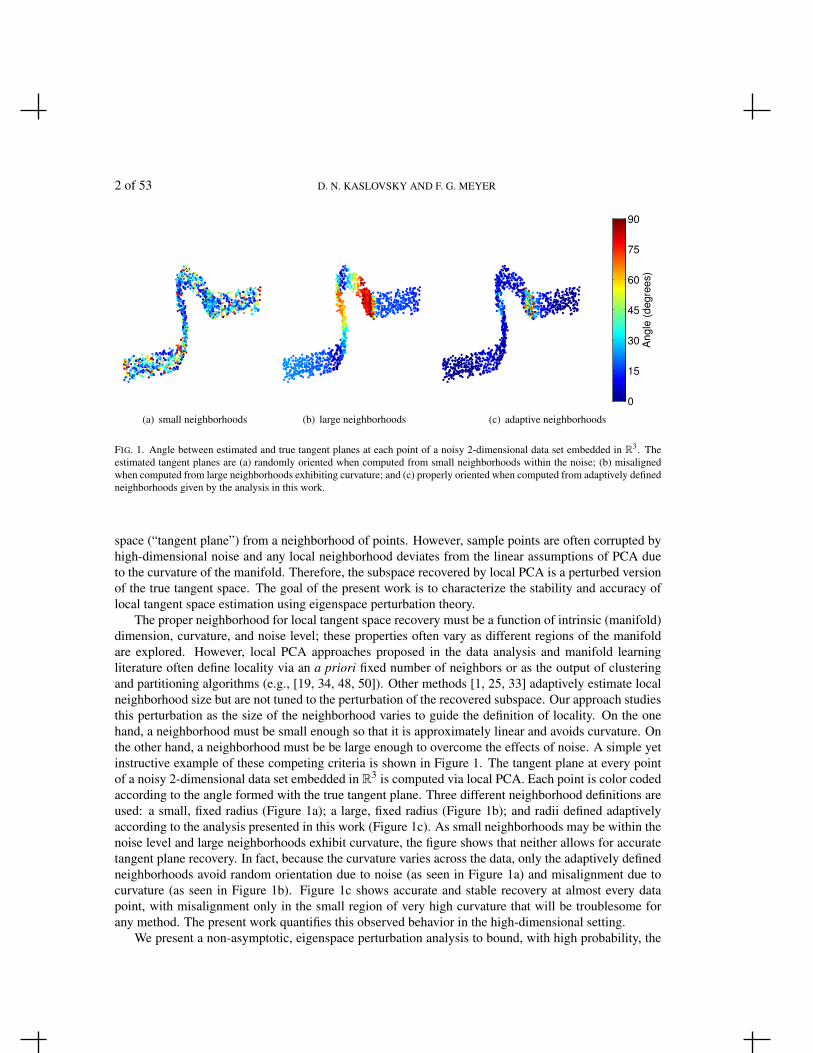
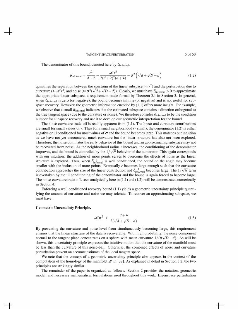
FIG. 1. Angle between estimated and true tangent planes at each point of a noisy 2-dimensional data set embedded in R3. Theestimated tangent planes are (a) randomly oriented when computed from small neighborhoods within the noise; (b) misalignedwhen computed from large neighborhoods exhibiting curvature; and (c) properly oriented when computed from adaptively definedneighborhoods given by the analysis in this work.
space (“tangent plane”) from a neighborhood of points. However, sample points are often corrupted byhigh-dimensional noise and any local neighborhood deviates from the linear assumptions of PCA dueto the curvature of the manifold. Therefore, the subspace recovered by local PCA is a perturbed versionof the true tangent space. The goal of the present work is to characterize the stability and accuracy oflocal tangent space estimation using eigenspace perturbation theory.
The proper neighborhood for local tangent space recovery must be a function of intrinsic (manifold)dimension, curvature, and noise level; these properties often vary as different regions of the manifoldare explored. However, local PCA approaches proposed in the data analysis and manifold learningliterature often define locality via an a priori fixed number of neighbors or as the output of clusteringand partitioning algorithms (e.g., [19, 34, 48, 50]). Other methods [1, 25, 33] adaptively estimate localneighborhood size but are not tuned to the perturbation of the recovered subspace. Our approach studiesthis perturbation as the size of the neighborhood varies to guide the definition of locality. On the onehand, a neighborhood must be small enough so that it is approximately linear and avoids curvature. Onthe other hand, a neighborhood must be be large enough to overcome the effects of noise. A simple yetinstructive example of these competing criteria is shown in Figure 1. The tangent plane at every pointof a noisy 2-dimensional data set embedded in R3 is computed via local PCA. Each point is color codedaccording to the angle formed with the true tangent plane. Three different neighborhood definitions areused: a small, fixed radius (Figure 1a); a large, fixed radius (Figure 1b); and radii defined adaptivelyaccording to the analysis presented in this work (Figure 1c). As small neighborhoods may be within thenoise level and large neighborhoods exhibit curvature, the figure shows that neither allows for accuratetangent plane recovery. In fact, because the curvature varies across the data, only the adaptively definedneighborhoods avoid random orientation due to noise (as seen in Figure 1a) and misalignment due tocurvature (as seen in Figure 1b). Figure 1c shows accurate and stable recovery at almost every datapoint, with misalignment only in the small region of very high curvature that will be troublesome forany method. The present work quantifies this observed behavior in the high-dimensional setting.
We present a non-asymptotic, eigenspace perturbation analysis to bound, with high probability, the
TANGENT SPACE PERTURBATION 3 of 53
angle between the recovered linear subspace and the true tangent space as the size of the local neighbor-hood varies. The analysis accurately tracks the subspace recovery error as a function of neighborhoodsize, noise, and curvature. Thus, we are able to adaptively select the neighborhood that minimizes thisbound, yielding the best estimate to the local tangent space from a large but finite number of noisymanifold samples. Further, the behavior of this bound demonstrates the non-trivial existence of suchan optimal scale. We also introduce a geometric uncertainty principle quantifying the limits of noise-curvature perturbation for tangent space recovery.
An important technical matter that one needs to address when analyzing points that are sampledfrom a manifold blurred with Gaussian noise concerns the probability distribution of the noisy samples.Indeed, after perturbation with Gaussian noise, the probability density function of the noisy points canbe expressed as the convolution of the probability density function of the clean points on the manifoldwith a Gaussian kernel. Geometrically, the points are diffused into a tube around the manifold, and thecorresponding density of the points is thinned. This concept has been studied in great detail in [26, 27]as well as in [12, 32]. The practical implication of these studies is that concentration of measure helpsus to guarantee that the volume of noisy points in a ball centered on the clean manifold can be estimatedfrom the volume of the corresponding ball of clean points, provided one applies a correction of theradius. We take advantage of these ideas in our analysis by replacing the ball of noisy points in thetube with a ball of similar volume extracted from the clean manifold, perturbed by Gaussian noise. Weintroduce the resulting, necessary modification to the radii in Section 5. A related issue concerns thedetermination of the point x0 about which we estimate the tangent plane. From a practical perspective,one can only observe noisy samples, and it is therefore reasonable that the perturbation bound shouldaccount for the fact that the analysis cannot be centered around the clean manifold. The expected effectof this additional source of uncertainty has been explored in detail in [26, 27]. In this paper, we proposea different approach. We devise a plug-in method to estimate a clean point x0 on the manifold using theobserved noisy data. As a result, the theoretical analysis can proceed assuming that x0 is given by anoracle. Our experiments confirm that the local origin x0 on the manifold can be estimated from the noisyneighborhood of observed points and that the perturbation error can be accurately tracked in practice. Inaddition, we expect this novel denoising algorithm to provide a universal tool for the analysis of noisypoint cloud data.
Our analysis is related to the very recent work of Tyagi, et al. [43], in which neighborhood sizeand sampling density conditions are given to ensure a small angle between the PCA subspace and thetrue tangent space of a noise-free manifold. Results are extended to arbitrary smooth embeddings of themanifold model, which we do not consider. In contrast, we envision the scenario in which no control isgiven over the sampling and explore the case of data sampled according to a fixed density and corruptedby high-dimensional noise. Crucial to our results is a careful analysis of the interplay between theperturbation due to noise and the perturbation due to curvature. Nonetheless, our results can be shownto recover those of [43] in the noise-free setting. Our approach is also similar to the analysis presentedby Nadler in [31], who studies the finite-sample properties of the PCA spectrum. Through matrixperturbation theory, [31] examines the angle between the leading finite-sample-PCA eigenvector andthat of the leading population-PCA eigenvector. As a linear model is assumed, perturbation results fromnoise only. Despite this difference, the two analyses utilize similar techniques to bound the effects ofperturbation on the PCA subspace and our results recover those of [31] in the curvature-free setting.
Application of multiscale PCA for geometric analysis of data sets has also been studied in [2, 9, 10,46]. In parallel to our work [20–22, 28], Maggioni and coauthors have developed results [3, 26, 27]addressing similar questions as those examined in this paper. These results are discussed above as wellas in more detail in Section 5 and Section 6. Other recent related works include that of Singer and
4 of 53 D. N. KASLOVSKY AND F. G. MEYER
Wu [40], who use local PCA to build a tangent plane basis and give an analysis for the neighborhoodsize to be used in the absence of noise. Using the hybrid linear model, Zhang, et al. [49] assume dataare samples from a collection of “flats” (affine subspaces) and choose an optimal neighborhood sizefrom which to recover each flat by studying the least squares approximation error in the form of Jones’β -number (see [17] and also [7] in which this idea is used for curve denoising). Finally, an analysis ofnoise and curvature for normal estimation of smooth curves and surfaces in R2 and R3 is presented byMitra, et al. [29] with application to computer graphics.
1.2 Overview of the Results
We consider the problem of recovering the best approximation to a local tangent space of a nonlineard-dimensional Riemannian manifold M from noisy samples presented in dimension D > d. Workingabout a reference point x0, an approximation to the tangent space of M at x0 is given by the span ofthe top d eigenvectors of the centered data covariance matrix (where “top” refers to the d eigenvectorsor singular vectors associated with the d largest eigenvalues or singular values). The question becomes:how many neighbors of x0 should be used (or in how large of a radius about x0 should we work) torecover the best approximation? We will often use the term “scale” to refer to this neighborhood size orradius.
To answer this question, we consider the perturbation of the eigenvectors spanning the estimatedtangent space in the context of the “noise-curvature trade-off.” To balance the effects of noise andcurvature (as observed in the example of the previous subsection, Figure 1), we seek a scale largeenough to be above the noise level but still small enough to avoid curvature. This scale reveals a linearstructure that is sufficiently decoupled from both the noise and the curvature to be well approximated bya tangent plane. At this scale, the recovered eigenvectors span a subspace corresponding very closely tothe true tangent space of the manifold at x0. We note that the concept of noise-curvature trade-off hasbeen a subject of interest for decades in dynamical systems theory [9].
The main result of this work is a bound on the angle between the computed and true tangent spaces.Define P to be the orthogonal projector onto the true tangent space and let P be the orthogonal projectorconstructed from the d-dimensional eigenspace of the neighborhood covariance matrix. Then the dis-tance ‖P−P‖2
F corresponds to the sum of the squared sines of the principal angles between the computedand true tangent spaces and we use eigenspace perturbation theory to bound this norm. Momentarilyneglecting probability-dependent constants to ease the presentation, the first-order approximation of thisbound has the following form:
Informal Main Result.
‖P− P‖F 6
2√
2√N
[K(+)r3 +σ
√d(D−d)
(σ + r√
d+2+ K 1/2r2
(d+2)√
2(d+4)
)]r2
d+2 −K r4
2(d+2)2(d+4) −σ2(√
d +√
D−d) , (1.1)
where r is the radius (measured in the tangent plane) of the neighborhood containing N points, σ is thenoise level, and K(+) and K are functions of curvature.
To aid the interpretation, we note that K(+) corresponds to the Frobenius norm of the matrix of principalcurvatures and K has size 2d(D−d)κ2 in the case where all principal curvatures are equal to κ . Thequantities N, r, σ , K(+), and K , as well as the sampling assumptions are more formally defined inSections 2 and 3, and the formal result is presented in Section 3.
TANGENT SPACE PERTURBATION 5 of 53
The denominator of this bound, denoted here by δinformal,
δinformal =r2
d +2− K r4
2(d +2)2(d +4)−σ
2(√
d +√
D−d)
(1.2)
quantifies the separation between the spectrum of the linear subspace (≈ r2) and the perturbation due tocurvature (≈K r4) and noise (≈σ2(
√d+√
D−d)). Clearly, we must have δinformal > 0 to approximatethe appropriate linear subspace, a requirement made formal by Theorem 3.1 in Section 3. In general,when δinformal is zero (or negative), the bound becomes infinite (or negative) and is not useful for sub-space recovery. However, the geometric information encoded by (1.1) offers more insight. For example,we observe that a small δinformal indicates that the estimated subspace contains a direction orthogonal tothe true tangent space (due to the curvature or noise). We therefore consider δinformal to be the conditionnumber for subspace recovery and use it to develop our geometric interpretation for the bound.
The noise-curvature trade-off is readily apparent from (1.1). The linear and curvature contributionsare small for small values of r. Thus for a small neighborhood (r small), the denominator (1.2) is eithernegative or ill conditioned for most values of σ and the bound becomes large. This matches our intuitionas we have not yet encountered much curvature but the linear structure has also not been explored.Therefore, the noise dominates the early behavior of this bound and an approximating subspace may notbe recovered from noise. As the neighborhood radius r increases, the conditioning of the denominatorimproves, and the bound is controlled by the 1/
√N behavior of the numerator. This again corresponds
with our intuition: the addition of more points serves to overcome the effects of noise as the linearstructure is explored. Thus, when δ
−1informal is well conditioned, the bound on the angle may become
smaller with the inclusion of more points. Eventually r becomes large enough such that the curvaturecontribution approaches the size of the linear contribution and δ
−1informal becomes large. The 1/
√N term
is overtaken by the ill conditioning of the denominator and the bound is again forced to become large.The noise-curvature trade-off, seen analytically here in (1.1) and (1.2), will be demonstrated numericallyin Section 4.
Enforcing a well conditioned recovery bound (1.1) yields a geometric uncertainty principle quanti-fying the amount of curvature and noise we may tolerate. To recover an approximating subspace, wemust have:
Geometric Uncertainty Principle.
K σ2 <
d +42(√
d +√
D−d)(1.3)
By preventing the curvature and noise level from simultaneously becoming large, this requirementensures that the linear structure of the data is recoverable. With high probability, the noise componentnormal to the tangent plane concentrates on a sphere with mean curvature 1/(σ
√D−d). As will be
shown, this uncertainty principle expresses the intuitive notion that the curvature of the manifold mustbe less than the curvature of this noise-ball. Otherwise, the combined effects of noise and curvatureperturbation prevent an accurate estimate of the local tangent space.
We note that the concept of a geometric uncertainty principle also appears in the context of thecomputation of the homology of the manifold M in [32]. As explained in detail in Section 3.2, the twoprinciples are strikingly similar.
The remainder of the paper is organized as follows. Section 2 provides the notation, geometricmodel, and necessary mathematical formulations used throughout this work. Eigenspace perturbation
6 of 53 D. N. KASLOVSKY AND F. G. MEYER
theory is reviewed in this section. The main results are stated formally in Section 3. We demonstratethe accuracy of our results and test the sensitivity to errors in parameter estimation in Section 4. Section5 presents the modifications that are needed to account for the sampling density of the noisy points,and introduces two plug-in estimates that can be used in practice to apply the theoretical results ofSection 3 to a real data set. We conclude in Section 6 with a discussion of the relationship to previouslyestablished results and further algorithmic considerations. Technical results and proofs are presented inthe appendices.
2. Mathematical Preliminaries
2.1 Geometric Data Model
A d-dimensional Riemannian manifold of codimension 1 may be described locally about a referencepoint x0 by the surface y = f (`1, . . . , `d), where `i is a coordinate in the tangent plane, Tx0M , to themanifold at x0. After translating x0 to the origin, we have
x0 = [0 0 · · · 0]T ,
and a rotation of the coordinate system can align the coordinate axes with the principal directions asso-ciated with the principal curvatures at x0. Aligning the coordinate axes with the plane tangent to M atx0 gives a local quadratic approximation to the manifold. Using this choice of coordinates, the manifoldmay be described locally [13] by the Taylor series of f at x0:
y = f (`1, . . . , `d) =12(κ1`
21 + · · ·+κd`
2d)+o
(`2
1 + · · ·+ `2d), (2.1)
where κ1, . . . ,κd are the principal curvatures of M at x0. In this coordinate system, a point x in aneighborhood of x0 has the form
x = [`1 `2 · · · `d f (`1, . . . , `d)]T .
Generalizing to a d-dimensional manifold of arbitrary codimension in RD, there exist (D−d) functions
fi(`) =12(κ
(i)1 `2
1 + · · ·+κ(i)d `2
d)+o(`2
1 + · · ·+ `2d), (2.2)
for i = (d+1), . . . ,D, with κ(i)1 , . . . ,κ
(i)d representing the principal curvatures in the ith normal direction
at x0. Then, given the coordinate system aligned with the principal directions, a point in a neighbor-hood of x0 has coordinates [`1, . . . , `d , fd+1, . . . , fD]. We truncate the Taylor expansion (2.2) and use thequadratic approximation
fi(`) =12(κ
(i)1 `2
1 + · · ·+κ(i)d `2
d), (2.3)
i = (d +1), . . . ,D, to describe the manifold locally.Consider now discrete samples from M obtained by uniformly sampling the first d coordinates
(`1, . . . , `d) in the tangent space inside Bdx0(r), the d-dimensional ball of radius r centered at x0, with
the remaining (D− d) coordinates given by (2.3). Because we are sampling from a noise-free linearsubspace, the number of points N captured inside Bd
x0(r) is a function of the sampling density ρ:
N = ρvdrd , (2.4)
TANGENT SPACE PERTURBATION 7 of 53
where vd is the volume of the d-dimensional unit ball. The sampled points are assumed to be in generallinear position, a standard assumption when sampling from a linear subspace (see Remark 2.3).
Finally, we assume the sample points of M are contaminated with an additive Gaussian noise vectore drawn from the N
(0,σ2ID
)distribution. Each sample x is a D-dimensional vector, and N such
samples may be stored as columns of a matrix X ∈ RD×N . The coordinate system above allows thedecomposition of x into its linear (tangent plane) component `, its quadratic (curvature) component c,and noise e, three D-dimensional vectors
`= [`1 `2 · · · `d 0 · · · 0]T (2.5)
c = [0 · · · 0 cd+1 · · · cD]T (2.6)
e = [e1 e2 · · · eD]T (2.7)
such that the last (D− d) entries of c are of the form ci = fi(`), i = (d + 1), . . . ,D. We may store theN samples of `, c, and e as columns of matrices L, C, E, respectively, such that our data matrix isdecomposed as
X = L+C+E. (2.8)
The true tangent space we wish to recover is given by the PCA of L. Because we do not have directaccess to L, we work with X as a proxy, and instead recover a subspace spanned by the correspondingeigenvectors of XXT . We will study how close this recovered invariant subspace of XXT is to thecorresponding invariant subspace of LLT as a function of scale. Throughout this work, scale refers tothe number of points N in the local neighborhood within which we perform PCA. Given a fixed densityof points, scale may be equivalently quantified as the radius r about the reference point x0 defining thelocal neighborhood.
REMARK 2.1 Of course it is unrealistic for the data to be observed in the described coordinate system.As noted, we may use a rotation to align the coordinate axes with the principal directions associated withthe principal curvatures. Doing so allows us to write (2.3) as well as (2.8). Because we will ultimatelyquantify the norm of each matrix using the unitarily-invariant Frobenius norm, this rotation will notaffect our analysis. We therefore proceed by assuming that the coordinate axes align with the principaldirections.
REMARK 2.2 Equation (2.3) represents an exact quadratic embedding of M . While it may be interest-ing to consider more general embeddings, as is done for the noise-free case in [43], a Taylor expansionfollowed by rotation and translation will result in an embedding of the form (2.2). Noting that thenumerical results of [43] indicate no loss in accuracy when truncating higher-order terms, proceedingwith an analysis of (2.3) remains sufficiently general.
REMARK 2.3 In a non-pathological configuration (e.g., points observed in general linear position), onlyd+1 sample points are needed to ensure that the top d eigenvectors of LLT span the true tangent space. Ithas been noted in the literature (e.g., [38, 44]) that O(d logd) points should be sampled for the empiricalcovariance matrix to be close in norm to the population covariance, with high probability. Strictlyenforcing this sampling condition is a very mild requirement for our setting, in which the samplingdensity ρ (see equation (2.4)) is usually large and the extra logarithmic factor of d is easily achieved.Further, this logarithmic factor is implicitly present in our analysis as a consequence of the lower boundon the smallest eigenvalue of LLT (see Appendix A.1). We also note that we do not intend to analyzethe extremely small scales (very small N) where finite sample effects create instability and prevent ameaningful analysis.
8 of 53 D. N. KASLOVSKY AND F. G. MEYER
2.2 Perturbation of Invariant Subspaces
Given the decomposition of the data (2.8), we have
XXT = LLT +CCT +EET +LCT +CLT +LET +ELT +CET +ECT . (2.9)
We introduce some notation to account for the centering required by PCA. Define the sample mean ofN realizations of random vector m as
m =1N
N
∑i=1
m(i), (2.10)
where m(i) denotes the ith realization. Letting 1N represent the column vector of N ones, define
M = m1TN (2.11)
to be the matrix with N copies of m as its columns. Finally, let M denote the centered version of M:
M = M−M. (2.12)
Then we have
X XT = LLT +CCT + EET + LCT +CLT + LET + ELT +CET + ECT . (2.13)
The problem may be posed as a perturbation analysis of invariant subspaces. Rewrite (2.9) as
1N
XXT =1N
LLT +∆ , (2.14)
where∆ =
1N(CCT + EET + LCT +CLT + LET + ELT +CET + ECT ) (2.15)
is the perturbation that prevents us from working directly with LLT . The dominant eigenspace of X XT
is therefore a perturbed version of the dominant eigenspace of LLT . Seeking to minimize the effect ofthis perturbation, we look for the scale N∗ (equivalently r∗) at which the dominant eigenspace of X XT
is closest to that of LLT . Before proceeding, we review material on the perturbation of eigenspacesrelevant to our analysis. The reader familiar with this topic is invited to skip directly to Theorem 2.1.
The distance between two subspaces of RD can be defined as the spectral norm of the differencebetween their respective orthogonal projectors [15]. As we will always be considering two equidimen-sional subspaces, this distance is equal to the sine of the largest principal angle between the subspaces.To control all such principal angles, we state our results using the Frobenius norm of this difference.Our goal is therefore to control the behavior of ‖P− P‖F , where P and P are the orthogonal projectorsonto the subspaces computed from L and X , respectively.
The norm ‖P− P‖F may be bounded by the classic sinΘ theorem of Davis and Kahan [4]. Wewill use a version of this theorem presented by Stewart (Theorem V.2.7 of [41]), modified for ourspecific purpose. First, we establish some notation, following closely that found in [41]. Consider theeigendecompositions
1N
LLT =UΛUT = [U1 U2]
[Λ1
Λ2
][U1 U2]
T , (2.16)
1N
XXT = UΛUT = [U1 U2]
[Λ1
Λ2
][U1 U2]
T , (2.17)
TANGENT SPACE PERTURBATION 9 of 53
such that the columns of U are the eigenvectors of 1N LLT and the columns of U are the eigenvectors of
1N X XT . The eigenvalues of 1
N LLT are arranged in descending order as the entries of diagonal matrix Λ .The eigenvalues are also partitioned such that diagonal matrices Λ1 and Λ2 contain the d largest entriesof Λ and the (D− d) smallest entries of Λ , respectively. The columns of U1 are those eigenvectorsassociated with the d eigenvalues in Λ1, the columns of U2 are those eigenvectors associated with the(D−d) eigenvalues in Λ2, and the eigendecomposition of 1
N X XT is similarly partitioned. The subspacewe recover is spanned by the columns of U1 and we wish to have this subspace as close as possible to thetangent space spanned by the columns of U1. The orthogonal projectors onto the tangent and computedsubspaces, P and P respectively, are given by
P =U1UT1 and P = U1UT
1 .
Define λd to be the dth largest eigenvalue of 1N LLT , or the last entry on the diagonal of Λ1. This
eigenvalue corresponds to variance in a tangent space direction.We are now in position to state the theorem. Note that we have made use of the fact that the columns
of U are the eigenvectors of LLT , that Λ1,Λ2 are Hermitian (diagonal) matrices, and that the Frobeniusnorm is used to measure distances. The reader is referred to [41] for the theorem in its original form.
THEOREM 2.1 (Davis & Kahan [4], Stewart [41]) Let
δ = λd−∥∥UT
1 ∆U1∥∥
F −∥∥UT
2 ∆U2∥∥
F
and consider
• (Condition 1) δ > 0
• (Condition 2)∥∥UT
1 ∆U2∥∥
F
∥∥UT2 ∆U1
∥∥F < 1
4 δ 2.
Then, provided that conditions 1 and 2 hold,∥∥∥P− P∥∥∥
F6 2√
2
∥∥UT2 ∆U1
∥∥F
δ. (2.18)
It is instructive to consider the perturbation ∆ as an operator with range in RD and quantify its effecton the existing invariant subspaces. Consider first the idealized case where U1 is an invariant subspaceof ∆ , i.e., ∆ maps points from the column space of U1 to the column space of U1. Clearly, UT
2 ∆U1 = 0in this case as the subspace spanned by U1 remains invariant under the action of ∆ , and the perturbationangle is zero. In general, however, we cannot expect such an idealized restriction for the range of∆ and we therefore expect that ∆U1 will have a component that is normal to the tangent space. Thenumerator ‖UT
2 ∆U1‖F of (2.18) measures this normal component, thereby quantifying the effect of theperturbation on the tangent space. Then ‖UT
1 ∆U1‖F measures the component that remains in the tangentspace after the action of ∆ . As this component does not contain curvature, ‖UT
1 ∆U1‖F corresponds tothe spectrum of the noise projected in the tangent space. Similarly, ‖UT
2 ∆U2‖F measures the spectrumof the curvature and noise perturbation normal to the tangent space. Thus, when ∆ leaves the columnspace of U1 mostly unperturbed (i.e., ‖UT
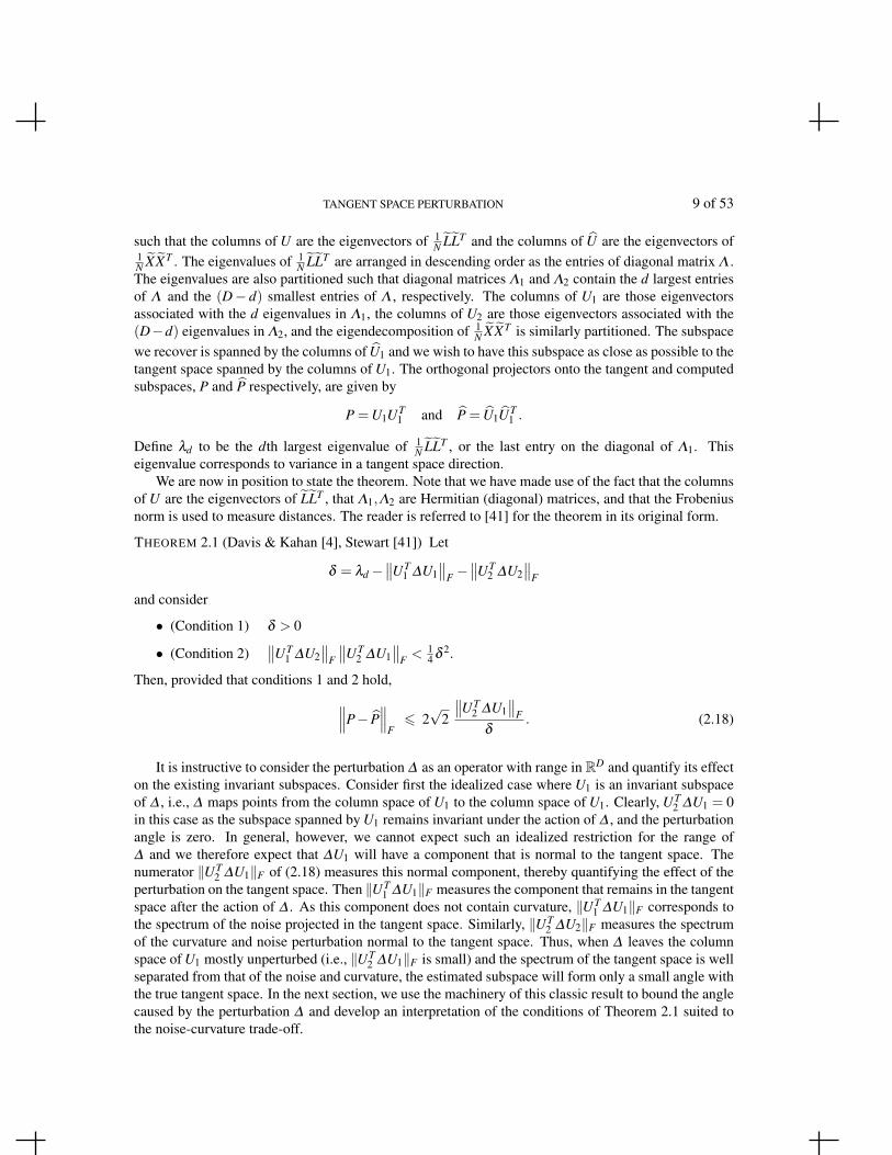
2 ∆U1‖F is small) and the spectrum of the tangent space is wellseparated from that of the noise and curvature, the estimated subspace will form only a small angle withthe true tangent space. In the next section, we use the machinery of this classic result to bound the anglecaused by the perturbation ∆ and develop an interpretation of the conditions of Theorem 2.1 suited tothe noise-curvature trade-off.
10 of 53 D. N. KASLOVSKY AND F. G. MEYER
3. Main Results
Given the framework for analysis developed above, the terms appearing in the statement of Theorem 2.1(∥∥UT
1 ∆U1∥∥
F ,∥∥UT
2 ∆U2∥∥
F ,∥∥UT
2 ∆U1∥∥
F ,∥∥UT
1 ∆U2∥∥
F , and λd) must be controlled. We notice that ∆ is asymmetric matrix, so that
∥∥UT1 ∆U2
∥∥F =
∥∥UT2 ∆U1
∥∥F . Using the triangle inequality and the geometric
constraintsUT
1 C = 0 and UT2 L = 0, (3.1)
the norms may be controlled by bounding the contribution of each term in the perturbation ∆ :
∥∥UT1 ∆U1
∥∥F 6 2
∥∥∥∥UT1
1N
LETU1
∥∥∥∥F+
∥∥∥∥UT1
1N
EETU1
∥∥∥∥F,
∥∥UT2 ∆U2
∥∥F 6
∥∥∥∥UT2
1N
CCTU2
∥∥∥∥F+2∥∥∥∥UT
21N
CETU2
∥∥∥∥F+
∥∥∥∥UT2
1N
EETU2
∥∥∥∥F,
∥∥UT2 ∆U1
∥∥F 6
∥∥∥∥UT2
1N
CLTU1
∥∥∥∥F+
∥∥∥∥UT2
1N
ELTU1
∥∥∥∥F+
∥∥∥∥UT2
1N
CETU1
∥∥∥∥F+
∥∥∥∥UT2
1N
EETU1
∥∥∥∥F.
Importantly, we seek control over each (right-hand side) term in the finite-sample regime, as we assumea possibly large but finite number of sample points N. Therefore, bounds are derived through a carefulanalysis employing concentration results and techniques from non-asymptotic random matrix theory.The technical analysis is presented in the appendix and proceeds by analyzing three distinct cases: thecovariance of bounded random matrices, unbounded random matrices, and the interaction of boundedand unbounded random matrices. The eigenvalue λd is bounded again using random matrix theory.In all cases, care is taken to ensure that bounds hold with high probability that is independent of theambient dimension D.
REMARK 3.1 Other, possibly tighter, avenues of analysis may be possible for some of the bounds pre-sented in the appendix. However, the presented analysis avoids large union bounds and dependence onthe ambient dimension to state results holding with high probability. Alternative analyses are possible,often sacrificing probability to exhibit sharper concentration. We proceed with a theoretical analysisholding with the highest probability while maintaining accurate results.
3.1 Bounding the Angle Between Subspaces
We are now in position to apply Theorem 2.1 and state our main result. First, we make the followingdefinitions involving the principal curvatures:
Ki =d
∑n=1
κ(i)n , K =
(D
∑i=d+1
K2i
) 12
, (3.2)
Ki jnn =
d
∑n=1
κ(i)n κ
( j)n , Ki j
mn =d
∑m,n=1m 6=n
κ(i)m κ
( j)n , (3.3)
and
K =
[D
∑i=d+1
D
∑j=d+1
[(d +1)Ki j
nn−Ki jmn]2] 1
2
. (3.4)
TANGENT SPACE PERTURBATION 11 of 53
The constant Ki is the mean curvature (rescaled by a factor of d) in normal direction i, for (d+1)6 i6D.The curvature of the local model is quantified by K, which is a natural result of our use of the Frobeniusnorm, and K , which results from the expectation of the norm of the curvature covariance. Note thatKiK j = Ki j
nn +Ki jmn. We also define the constants
K(+)i =
(d
∑n=1|κ(i)
n |2) 1
2
, and K(+) =
(D
∑i=d+1
(K(+)i )2
) 12
(3.5)
to be used when strictly positive curvature terms are required.The main result is formulated in the appendix and makes the following benign assumptions on the
number of sample points N and the probability constants ξ and ξλ :
N > 4(max(√
d,√
D−d)+ξ ), ξ < 0.7√
d(D−d), and ξλ <3√
d +2
√N,
in addition to the requirement that N >O(d logd) for the points observed in general linear position (seeRemark 2.3). We note that the assumptions are easily satisfied as we envision a sampling density suchthat N is large (but finite). Further, the assumptions listed above are not crucial to the result but allowfor a more compact presentation.
THEOREM 3.1 (Main Result) Let
δ =r2
d +2− K r4
2(d +2)2(d +4)−σ
2(√
d +√
D−d)− 1√
Nζdenom(ξ ,ξλ ) (3.6)
and
β =1√N
[K(+)r3
ν(ξ )+σ√
d(D−d)η(ξ ,ξλ )+1√N
ζnumer(ξ )
]. (3.7)
If the following conditions hold (in addition to the benign assumptions stated above):
• (Condition 1) δ > 0,
• (Condition 2) β < 12 δ ,
then
∥∥∥P− P∥∥∥
F6
2√
2β
δ=
2√
2 1√N
[K(+)r3ν(ξ )+σ
√d(D−d)η(ξ ,ξλ )+
1√N
ζnumer(ξ )]
r2
d+2 −K r4
2(d+2)2(d+4) −σ2(√
d +√
D−d)− 1√
Nζdenom(ξ ,ξλ )
(3.8)
with probability greater than1−2de−ξ 2
λ −9e−ξ 2(3.9)
over the joint random selection of the sample points and random realization of the noise, where thefollowing definitions have been made to ease the presentation:
• geometric and noise terms
ν(ξ ) =12(d +3)(d +2)
p1(ξ ), (linear–curvature)
12 of 53 D. N. KASLOVSKY AND F. G. MEYER
η1 = σ , (noise)
η2(ξλ ) =r√
d +2p2(ξλ ), (linear–noise)
η3(ξ ) =K 1/2r2
(d +2)√
2(d +4)p5(ξ ), (curvature–noise)
η(ξ ,ξλ ) = p3(ξ ,√
d(D−d))[
η1 +η2(ξλ )+η3(ξ )
],
• finite sample correction terms (numerator)
ζ1(ξ ) =12
K(+)r3 p21(ξ ), (linear–curvature)
ζ2(ξ ) = σ2√
d(D−d)p3(ξ ,√
d(D−d))p4(ξ ,√
D−d), (noise)ζnumer(ξ ) = ζ1(ξ )+ζ2(ξ ),
• finite sample correction terms (denominator)
ζ3(ξλ ) =r2
d +2
[p0(ξλ )+
(2√N− 1
N3/2
)(1− p0(ξλ )√
N
)], (linear)
ζ4(ξ ) =(K(+))2r4
4
(p1(ξ )+
1√N
p21(ξ )
), (curvature)
ζ5(ξ ,ξλ ) = 2rσd√
d +2p2(ξλ )p3(ξ ,d), (linear–noise)
ζ6(ξ ) = 2K12 r2
σ(D−d)
(d +2)√
2(d +4)p3(ξ ,D−d)p5(ξ ), (curvature–noise)
ζ7(ξ ) =52
σ2[√
d p4(ξ ,√
d)+√
D−d p4(ξ ,√
D−d)], (noise)
ζdenom(ξ ,ξλ ) = ζ3(ξ )+ζ4(ξ )+ζ5(ξ ,ξλ )+ζ6(ξ )+ζ7(ξ ),
and
• probability-dependent terms (i.e., terms depending on the probability constants)
p0(ξ ) = ξ
√8(d +2)(1− 1
N ), p1(ξ ) =
(2+ξ
√2), p2(ξ ) =
(1+ξ
5√
d +2√N
),
p3(ξ ,ω) =
(1+
65
ξ
ω
), p4(ξ ,ω) =
(ω +ξ
√2),
p5(ξ ) =
(1+
1√N(K(+))2
2K(d +2)2(d +4)(p1(ξ )+
1√N
p21(ξ ))
)1/2
.
TANGENT SPACE PERTURBATION 13 of 53
Finally, we recall the relationship N = ρvdrd given by (2.4).
Proof. Condition 2 is simplified from its original statement in Theorem 2.1 by noticing that ∆ is asymmetric matrix so that
∥∥UT1 ∆U2
∥∥F =
∥∥UT2 ∆U1
∥∥F . Then, applying the norm bounds computed in the
appendix to Theorem 2.1 and choosing the probability constants
ξλd= ξλ1 = ξλ and ξcc = ξc` = ξe` = ξce = ξe1 = ξe2 = ξe3 = ξc = ξ (3.10)
yields the result.
The bound (3.8) will be demonstrated in Section 4 to accurately track the angle between the true andcomputed tangent spaces at all scales. We experimentally observe that the bound is, in general, eitherdecreasing (for the curvature-free case), increasing (for the noise-free case), or decreasing at small scalesand increasing at large scales (for the general case). We therefore expect to be able to locate a scale atwhich the bound is minimized. Based on this observation, the optimal scale, N∗, for tangent spacerecovery may be selected as the N for which (3.8) is minimized (an equivalent notion of the optimalscale may be given in terms of the neighborhood radius r). Note that the constants ξ and ξλ need to beselected to ensure that this bound holds with high probability. For example, setting ξ = 2 and ξλ = 2.75yields probabilities of 0.81, 0.80, and 0.76 when d = 3,10, and 50, respectively. We also note that theprobability given by (3.9) is more pessimistic than we expect in practice.
As introduced in Section 1.2, we may interpret δ−1 as the condition number for tangent spacerecovery. Noting that the denominator in (3.8) is a lower bound on δ , we analyze the condition numbervia the bounds for λd , ‖UT
1 ∆U1‖F , and ‖UT2 ∆U2‖F . Using these bounds in the Main Result (3.8), we
see that when δ−1 is small, we recover a tight approximation to the true tangent space. Likewise, whenδ−1 becomes large, the angle between the computed and true subspaces becomes large. The notion of anangle loses meaning as δ−1 tends to infinity, and we are unable to recover an approximating subspace.
Condition 1, requiring that the denominator be bounded away from zero, has an important geo-metric interpretation. As noted above, the conditioning of the subspace recovery problem improvesas δ becomes large. Condition 1 imposes that the spectrum corresponding to the linear subspace (λd)be well separated from the spectra of the noise and curvature perturbations encoded by ‖UT
1 ∆U1‖F +‖UT
2 ∆U2‖F . In this way, condition 1 quantifies our requirement that there exists a scale such that thelinear subspace is sufficiently decoupled from the effects of curvature and noise. When the spectra arenot well separated, the angle between the subspaces becomes ill defined. In this case, the approximat-ing subspace contains an eigenvector corresponding to a direction orthogonal to the true tangent space.Condition 2 is a technical requirement of Theorem 2.1. Provided that condition 1 is satisfied, we observethat a sufficient sampling density will ensure that Condition 2 is met. Further, we numerically observethat the Main Result (3.8) accurately tracks the subspace recovery error even in the case when condition2 is violated. In such a case, the bound may not remain as tight as desired but its behavior at all scalesremains consistent with the subspace recovery error tracked in our experiments.
Before numerically demonstrating our main result, we quantify the separation needed between thelinear structure and the noise and curvature with a geometric uncertainty principle.
3.2 Geometric Uncertainty Principle for Subspace Recovery
Condition 1 indeed imposes a geometric requirement for tangent space recovery. Solving for the rangeof scales for which condition 1 is satisfied and requiring the solution to be real yields the geometricuncertainty principle (1.3) stated in Section 1.2. We note that this result is derived using δinformal,defined in equation (1.2), as the full expression for δ does not allow for an algebraic solution.
14 of 53 D. N. KASLOVSKY AND F. G. MEYER
The geometric uncertainty principle (1.3) expresses a natural requirement for the subspace recoveryproblem, ensuring that the perturbation to the tangent space is not too large. Recall that, with highprobability, the noise orthogonal to the tangent space concentrates on a sphere with mean curvature1/(σ
√D−d). We therefore expect to require that the curvature of the manifold be less than the curva-
ture of this noise-ball. To compare the curvature of the manifold to that of the noise-ball, consider thecase where all principal curvatures of the manifold are equal, and denote them by κ . Then (1.3) requiresthat
κ <1
σ√
D−d
√√√√ d +4
4d(√
d +√
D−d) . (3.11)
Noting that, for d > 1, we haved +4
4d(√
d +√
D−d) < 1,
we see that the uncertainty principle (1.3) indeed requires that the mean curvature of the manifold beless than that of the perturbing noise-ball.
Intuitively, we might expect that the uncertainty principle would be of the form
(curvature)× (noise-ball radius)< 1.
However, (1.3) is, in fact, more restrictive than our intuition, as illustrated by (3.11). As only finite-sample corrections have been neglected in δinformal, (1.3) is of the correct order. Interestingly, this morerestrictive requirement for tangent space recovery is only accessible through the careful perturbationanalysis presented above and an estimate obtained by a more naive analysis would be too lax. Theauthors in [32] present an algorithm to compute the homology of a manifold from a data set of noisypoints. The authors assume that the data are clean samples from a manifold perturbed with (D− d)-dimensional Gaussian noise along the normal fibers. In the context of our model, this is equivalent toremoving the first d components of the noise vector. The authors prove that the algorithm computes,with high probability, the correct homology of M , provided that the noise variance σ2 satisfies
1R
<1
σ√
D−dc
√9−√
89√
8with c < 1. (3.12)
The parameter 1/R is an upper bound on all the principal curvatures (R is also known as the reach [8]).This condition is almost identical to (3.11). The geometric uncertainty principle (1.3) is clearly not anartifact of our analysis, but is deeply rooted in the geometric and topological understanding of noisymanifolds.
4. Experimental Results I: Validating the Theory
In this section we present an experimental study of the tangent space perturbation results given above.In particular, we demonstrate that the bound presented in the Main Result (Theorem 3.1) accuratelytracks the subspace recovery error at all scales. As this analytic result requires no decompositions ofthe data matrix, our analysis provides an efficient means for obtaining the optimal scale for tangentspace recovery. We first present a practical use of the Main Result, demonstrating its accuracy when theintrinsic dimensionality, curvature, and noise level are known. We then experimentally test the stabilityof the bound when these parameters are only imprecisely available, as is the case when they must be
TANGENT SPACE PERTURBATION 15 of 53
estimated from the data. Finally, we demonstrate the accurate estimation of the noise level and localcurvature.
4.1 Subspace Tracking and Recovery
We generate a data set sampled from a 3-dimensional manifold embedded in R20 according to the localmodel (2.3) by uniformly sampling N = 1.25×10⁶ points inside a ball of radius 1 in the tangent plane.Curvature and the standard deviation σ of the added Gaussian noise will be specified in each experiment.We compare our bound with the true subspace recovery error. The tangent plane at reference point x0 iscomputed at each scale N via PCA of the N nearest neighbors of x0. The true subspace recovery error‖P− P‖F is then computed at each scale. Note that computing the true error requires N SVDs. A “truebound” is computed by applying Theorem 2.1 after measuring each perturbation norm directly from thedata. While no SVDs are required, this true bound utilizes information that is not practically availableand represents the best possible bound that we can hope to achieve. We will compare the mean of thetrue error and mean of the true bound over 10 trials (with error bars indicating one standard deviation)to the bound given by our Main Result in Theorem 3.1, holding with probability greater than 0.8.
For the experiments in this section, the bound (3.8) is computed with full knowledge of the necessaryparameters. In our experience, we observe in practice (results not shown) that the deviation of theempirical eigenvalue λd from its expectation is insignificant over the entire range of relevant scalesand therefore neglect its correction term (derived using a Chernoff bound in Appendix A.1) for theexperiments. We further note that knowledge of d provides an exact expression for this expectationas no additional geometric information is encoded by λd . As the principle curvatures are known, wecompute a tighter bound for ‖UT
2 CLTU1‖F using K in place of K(+). Doing so only affects the heightof the curve; its trend as a function of scale is unchanged. In practice, the important information iscaptured by tracking the trend of the true error regardless of whether it provides an upper bound to anyrandom fluctuation of the data. In fact, the numerical results indicate that an accurate tracking of erroris possible even when condition 2 of Theorem 3.1 is violated.
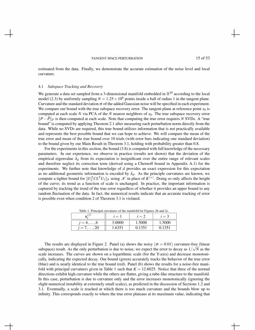
Table 1. Principal curvatures of the manifold for Figures 2b and 2c.
κ( j)i i = 1 i = 2 i = 3
j = 4, . . . ,6 3.0000 1.5000 1.5000j = 7, . . . ,20 1.6351 0.1351 0.1351
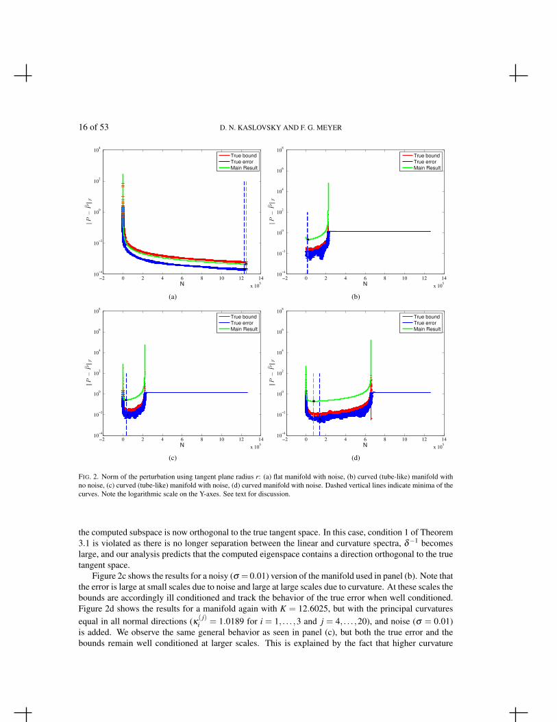
The results are displayed in Figure 2. Panel (a) shows the noisy (σ = 0.01) curvature-free (linearsubspace) result. As the only perturbation is due to noise, we expect the error to decay as 1/
√N as the
scale increases. The curves are shown on a logarithmic scale (for the Y-axis) and decrease monotoni-cally, indicating the expected decay. Our bound (green) accurately tracks the behavior of the true error(blue) and is nearly identical to the true bound (red). Panel (b) shows the results for a noise-free mani-fold with principal curvatures given in Table 1 such that K = 12.6025. Notice that three of the normaldirections exhibit high curvature while the others are flatter, giving a tube-like structure to the manifold.In this case, perturbation is due to curvature only and the error increases monotonically (ignoring theslight numerical instability at extremely small scales), as predicted in the discussion of Sections 1.2 and3.1. Eventually, a scale is reached at which there is too much curvature and the bounds blow up toinfinity. This corresponds exactly to where the true error plateaus at its maximum value, indicating that
16 of 53 D. N. KASLOVSKY AND F. G. MEYER
−2 0 2 4 6 8 10 12 14
x 105
10−4
10−2
100
102
104
N
‖P
−P‖F
True bound
True error
Main Result
(a)
−2 0 2 4 6 8 10 12 14
x 105
10−4
10−2
100
102
104
106
108
N
‖P
−P‖F
True bound
True error
Main Result
(b)
−2 0 2 4 6 8 10 12 14
x 105
10−4
10−2
100
102
104
106
108
N
‖P
−P‖F
True bound
True error
Main Result
(c)
−2 0 2 4 6 8 10 12 14
x 105
10−4
10−2
100
102
104
106
108
N
‖P
−P‖F
True bound
True error
Main Result
(d)
FIG. 2. Norm of the perturbation using tangent plane radius r: (a) flat manifold with noise, (b) curved (tube-like) manifold withno noise, (c) curved (tube-like) manifold with noise, (d) curved manifold with noise. Dashed vertical lines indicate minima of thecurves. Note the logarithmic scale on the Y-axes. See text for discussion.
the computed subspace is now orthogonal to the true tangent space. In this case, condition 1 of Theorem3.1 is violated as there is no longer separation between the linear and curvature spectra, δ−1 becomeslarge, and our analysis predicts that the computed eigenspace contains a direction orthogonal to the truetangent space.
Figure 2c shows the results for a noisy (σ = 0.01) version of the manifold used in panel (b). Note thatthe error is large at small scales due to noise and large at large scales due to curvature. At these scales thebounds are accordingly ill conditioned and track the behavior of the true error when well conditioned.Figure 2d shows the results for a manifold again with K = 12.6025, but with the principal curvaturesequal in all normal directions (κ( j)
i = 1.0189 for i = 1, . . . ,3 and j = 4, . . . ,20), and noise (σ = 0.01)is added. We observe the same general behavior as seen in panel (c), but both the true error and thebounds remain well conditioned at larger scales. This is explained by the fact that higher curvature
TANGENT SPACE PERTURBATION 17 of 53
is encountered at smaller scales for the manifold corresponding to panel (c) but is not encountereduntil larger scales in panel (d). Similar results are shown in Figure 3 for a 2-dimensional, noise-freesaddle (κ(3)
1 = 3,κ(3)2 =−3) embedded in R3, demonstrating an accurate bound for the case of principle
curvatures of mixed signs.The true bound (red) tightly tracks the true error (blue) and is tighter than our bound (green) in all
cases except for the curvature-free setting, where a difference on the order of 10−3 is observed. Thiscurvature-free bound may be understood by observing that the noise analysis is more precise than thatfor the curvature (see appendices) and that the height of the bound is controlled by the probability-dependent constants, which have been fixed across all plots for consistency. In fact, it is possible tochoose the probability-dependent constants much larger for the curvature-free setting without violatingCondition 2. Doing so increases the height of the bound (green) to match the height of the “true bound”(red) curve (result not shown). Note that a similar increase for nonzero curvature results in a curve thatviolates Condition 2.
In all of the presented experiments, the bound accurately tracks the behavior of the true error. Infact, the curves are shown to be parallel on a logarithmic scale, indicating that they differ only by mul-tiplicative constants. These observations further indicate that the triangle inequalities used in boundingthe norms ‖UT
m ∆Un‖F , m,n = 1,2, are reasonably tight. As no matrix decompositions are needed tocompute our bounds, we have efficiently tracked the tangent space recovery error. The dashed verticallines in Figure 2 indicate the locations of the minima of the true error curve (dashed blue) and the MainResult bound (dashed green). In general, we see agreement of the locations at which the minima occur,indicating the scale that will yield the optimal tangent space approximation. The minimum of the MainResult bound falls within a range of scales at which the true recovery error is stable. In particular, wenote that when the location of the bound’s minimum does not correspond with the minimum of thetrue error (such as in panel (d)), the discrepancy occurs at a range of scales for which the true error isquite flat. In fact, in panel (d), the difference between the error at the computed optimal scale and theerror at the true optimal scale is on the order of 10−2. Thus the angle between the computed and truetangent spaces will be less than half of a degree and the computed tangent space is stable in this rangeof scales. For a large data set it is impractical to examine every scale and one would instead most likelyuse a coarse sampling of scales. The true optimal scale would almost surely be missed by such a coarsesampling scheme. Our analysis indicates that despite missing the exact true optimum, we may recovera scale that yields an approximation to within a fraction of a degree of the optimum.
4.2 Sensitivity to Error in Parameters
As is often the case in practice, parameters such as intrinsic dimension, curvature, and noise level areunknown and must be estimated from the data. It is therefore important to experimentally test thesensitivity of tangent space recovery to errors in parameter estimation. In the following experiments, wetest the sensitivity to each parameter by tracking the optimal scale as one parameter is varied with theothers held fixed at their true values. For consistency across experiments, the optimal scale is reportedin terms of neighborhood radius and denoted by r∗. The relationship between neighborhood radius rand number of sample points N is defined by equation (2.4). In all experiments, we generate data setssampled from a 4-dimensional manifold embedded in R10 according to the local model (2.3).
Figure 4 shows that the optimal scale r∗ is sensitive to errors in the intrinsic dimension d. A dataset is sampled from a noisy, bowl-shaped manifold with equal principal curvatures in all directions. Weset the noise level σ = 0.01 and the principal curvatures κ
(i)j = 2 in panel (a) and κ
(i)j = 3 in panel (b).
18 of 53 D. N. KASLOVSKY AND F. G. MEYER
−1000 0 1000 2000 3000 4000 5000 6000−1
−0.5
0
0.5
1
1.5
2
2.5
3
N
‖P
−P‖F
True bound
True error
Main Result
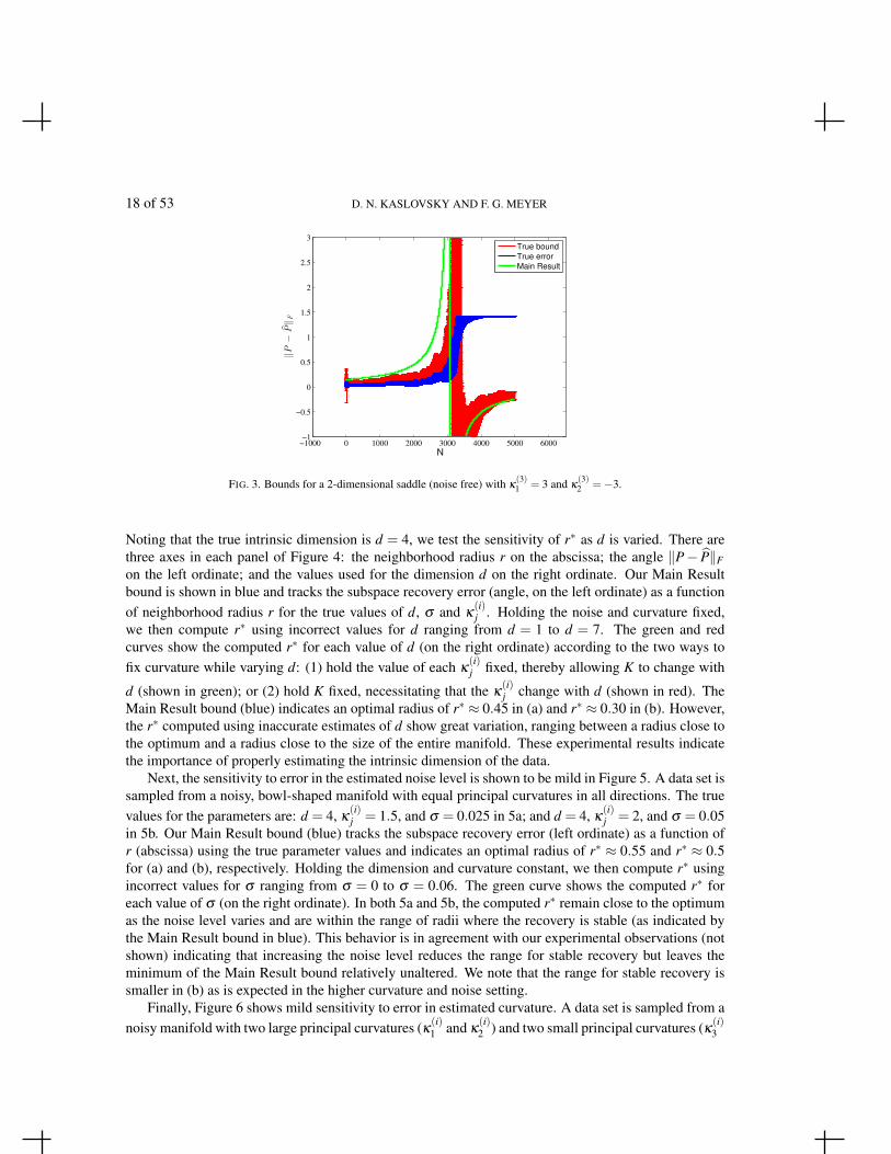
FIG. 3. Bounds for a 2-dimensional saddle (noise free) with κ(3)1 = 3 and κ
(3)2 =−3.
Noting that the true intrinsic dimension is d = 4, we test the sensitivity of r∗ as d is varied. There arethree axes in each panel of Figure 4: the neighborhood radius r on the abscissa; the angle ‖P− P‖Fon the left ordinate; and the values used for the dimension d on the right ordinate. Our Main Resultbound is shown in blue and tracks the subspace recovery error (angle, on the left ordinate) as a functionof neighborhood radius r for the true values of d, σ and κ
(i)j . Holding the noise and curvature fixed,
we then compute r∗ using incorrect values for d ranging from d = 1 to d = 7. The green and redcurves show the computed r∗ for each value of d (on the right ordinate) according to the two ways tofix curvature while varying d: (1) hold the value of each κ
(i)j fixed, thereby allowing K to change with
d (shown in green); or (2) hold K fixed, necessitating that the κ(i)j change with d (shown in red). The
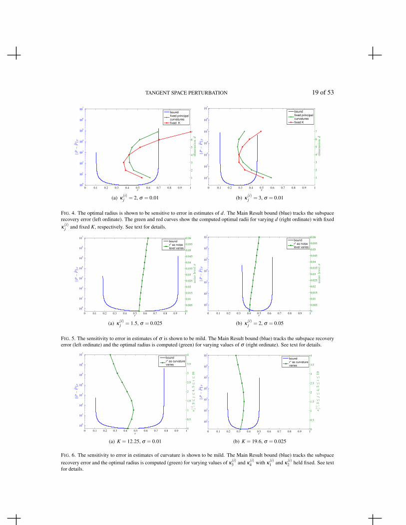
Main Result bound (blue) indicates an optimal radius of r∗ ≈ 0.45 in (a) and r∗ ≈ 0.30 in (b). However,the r∗ computed using inaccurate estimates of d show great variation, ranging between a radius close tothe optimum and a radius close to the size of the entire manifold. These experimental results indicatethe importance of properly estimating the intrinsic dimension of the data.
Next, the sensitivity to error in the estimated noise level is shown to be mild in Figure 5. A data set issampled from a noisy, bowl-shaped manifold with equal principal curvatures in all directions. The truevalues for the parameters are: d = 4, κ
(i)j = 1.5, and σ = 0.025 in 5a; and d = 4, κ
(i)j = 2, and σ = 0.05
in 5b. Our Main Result bound (blue) tracks the subspace recovery error (left ordinate) as a function ofr (abscissa) using the true parameter values and indicates an optimal radius of r∗ ≈ 0.55 and r∗ ≈ 0.5for (a) and (b), respectively. Holding the dimension and curvature constant, we then compute r∗ usingincorrect values for σ ranging from σ = 0 to σ = 0.06. The green curve shows the computed r∗ foreach value of σ (on the right ordinate). In both 5a and 5b, the computed r∗ remain close to the optimumas the noise level varies and are within the range of radii where the recovery is stable (as indicated bythe Main Result bound in blue). This behavior is in agreement with our experimental observations (notshown) indicating that increasing the noise level reduces the range for stable recovery but leaves theminimum of the Main Result bound relatively unaltered. We note that the range for stable recovery issmaller in (b) as is expected in the higher curvature and noise setting.
Finally, Figure 6 shows mild sensitivity to error in estimated curvature. A data set is sampled from anoisy manifold with two large principal curvatures (κ(i)
1 and κ(i)2 ) and two small principal curvatures (κ(i)
3
TANGENT SPACE PERTURBATION 19 of 53
0 0.1 0.2 0.3 0.4 0.5 0.6 0.7 0.8 0.9 110
0
101
102
103
104
105
106
107
r
‖P
−P‖F
1
2
3
4
5
6
7
dim
ensiond
boundfixed principalcurvaturesfixed K
(a) κ(i)j = 2, σ = 0.01
0 0.1 0.2 0.3 0.4 0.5 0.6 0.7 0.8 0.9 1
101
102
103
104
105
106
107
r
‖P
−P‖F
bound
fixed principalcurvatures
fixed K
1
2
3
4
5
6
7
dim
ensiond
(b) κ(i)j = 3, σ = 0.01
FIG. 4. The optimal radius is shown to be sensitive to error in estimates of d. The Main Result bound (blue) tracks the subspacerecovery error (left ordinate). The green and red curves show the computed optimal radii for varying d (right ordinate) with fixedκ(i)j and fixed K, respectively. See text for details.
0 0.1 0.2 0.3 0.4 0.5 0.6 0.7 0.8 0.9 1
100
101
102
103
104
105
106
107
r
‖P
−P‖F
bound
r* as noise
level varies
0
0.005
0.01
0.015
0.02
0.025
0.03
0.035
0.04
0.045
0.05
0.055
0.06
noiselevelσ
(a) κ(i)j = 1.5, σ = 0.025
0 0.1 0.2 0.3 0.4 0.5 0.6 0.7 0.8 0.9 1
101
102
103
104
105
106
107
r
‖P
−P‖F
bound
r* as noise
level varies
0
0.005
0.01
0.015
0.02
0.025
0.03
0.035
0.04
0.045
0.05
0.055
0.06
noiselevelσ
(b) κ(i)j = 2, σ = 0.05
FIG. 5. The sensitivity to error in estimates of σ is shown to be mild. The Main Result bound (blue) tracks the subspace recoveryerror (left ordinate) and the optimal radius is computed (green) for varying values of σ (right ordinate). See text for details.
0 0.1 0.2 0.3 0.4 0.5 0.6 0.7 0.8 0.9 1
100
101
102
103
104
105
106
107
r
‖P
−P‖F
bound
r* as curvature
varies
0
0.5
1
1.5
2
2.5
3
3.5
4
κ(i)
j,3≤
j≤
4,5≤
i≤
10
(a) K = 12.25, σ = 0.01
0 0.1 0.2 0.3 0.4 0.5 0.6 0.7 0.8 0.9 1
101
102
103
104
105
106
107
r
‖P
−P‖F
bound
r* as curvature
varies
0
0.5
1
1.5
2
2.5
3
3.5
4
κ(i)
j,3≤
j≤
4,5≤
i≤
10
(b) K = 19.6, σ = 0.025
FIG. 6. The sensitivity to error in estimates of curvature is shown to be mild. The Main Result bound (blue) tracks the subspacerecovery error and the optimal radius is computed (green) for varying values of κ
(i)3 and κ
(i)4 with κ
(i)1 and κ
(i)2 held fixed. See text
for details.
20 of 53 D. N. KASLOVSKY AND F. G. MEYER
and κ(i)4 ) in each normal direction i. This tube-like geometry provides more insight for sensitivity to error
in curvature by avoiding the more stable case where all principal curvatures are equal. The true valuesfor the parameters are: d = 4, σ = 0.01, κ
(i)1 = κ
(i)2 = 2, and κ
(i)3 = κ
(i)4 = 0.5 for 56 i6 10 in (a); and
d = 4, σ = 0.025, κ(i)1 = κ
(i)2 = 3, and κ
(i)3 = κ
(i)4 = 1 for 56 i6 10 in (b). Our Main Result bound (blue)
tracks the subspace recovery error (left ordinate) as a function of r (abscissa) using the true parametervalues and indicates an optimal radius of r∗ ≈ 0.45 and r∗ ≈ 0.35 for (a) and (b), respectively. Holdingthe dimension, noise level, and large principal curvatures κ
(i)1 and κ
(i)2 constant, we then compute the
r∗ using incorrect values for the smaller principal curvatures κ(i)3 and κ
(i)4 , 56 i6 10. The green curve
shows the r∗ computed for values of κ(i)3 = κ
(i)4 indicated on the right ordinate, 56 i6 10. The computed
r∗ remain within the range of radii where the recovery is stable (as indicated by the Main Result boundin blue) in both (a) and (b). We observe less variation in the higher curvature and higher noise caseshown in 6b. In this case, the larger principal curvatures anchor the bound, leaving r∗ less sensitive toerror in the estimated smaller principal curvatures. As can be expected, experimental results (not shown)indicate that r∗ is sensitive to perturbations of these anchoring, large principal curvatures.
5. Practical Application & Experimental Results II
With the purpose of providing perturbation bounds that can be used in practice, we provide in thissection the algorithmic tools that make it possible to directly apply the theoretical results of Section 3 toa real dataset.
The first tool is a “translation rule” to compare distances measured in the tangent plane Tx0M anddistances in RD: given a point x at a distance R from the origin, we provide an estimate, r(R), ofthe distance of the projection of x in Tx0M to the origin x0. The second tool is a plug-in method tocompute a “clean estimate”, x0, of the point x0 on M that serves as the origin of the coordinate systemin our analysis. Equipped with these two tools, the practitioner can compute the perturbation bound asa function of the radius R measured from x0 in the ambient space RD.
5.1 Effective Distance in the Tangent Plane Tx0M
Our Main Result, Theorem 3.1, is presented in terms of the radius r corresponding to the distance fromthe origin x0 of a point’s noise-free tangential component. Because r cannot be observed in practice,we provide an estimate r(R) of r for any point x at distance R from the origin. In the presentation thatfollows, we assume oracle knowledge of the local origin x0 ∈M ; recovery of this origin is addressed inthe next section.
As previously introduced, a point x in a neighborhood of x0 may be decomposed as x = x0+`+c+eand we recognize r2 = ‖`‖2. To explore the relationship between r and R, we compute
R2 = ‖x− x0‖2 = ‖x0 + `+ c+ e− x0‖2 = r2 +‖c‖2 +‖e‖2 +2〈`+ c,e〉, (5.1)
where we use that 〈`,c〉= 0. The terms on the right hand side depend on the realizations of the samplepoint x and noise e. To understand their sizes, we compute in expectation,
E[‖c‖2] = γr4, E[‖e‖2] = σ2D, and E[〈`+ c,e〉] = 0,
where
γ =∑
Di=d+1 3Kii
nn +Kiimn
2(d +2)(d +4). (5.2)
TANGENT SPACE PERTURBATION 21 of 53
Injecting these terms into (5.1), we solve for positive and real r and arrive at an approximation r(R) ofthe (tangent plane) radius r given the observable (ambient) radius R:
r(R) =
√12γ
(−1+
√1+4γ(R2−σ2D)
). (5.3)
REMARK 5.1 Another approach to determine the relationship between r and R proceeds as follows. Wecalculate the volume of the d-dimensional ball Bd
x0(r) given by the pre-image of the points in the ball
BDx0(R) of radius R in RD, and use this volume to derive an effective radius r.In the noise-free case, we can get some insight into this problem using a result from Gray [14] that
gives the volume of a geodesic ball BMx0(ω) on M centered at x0 as a function of the radius ω measured
along the manifold. We have
V (BMx0(ω)) = ω
dvd
(1− S(x0)
6(n+2)ω
2 +o(ω2)
),
where S(x0) is the scalar curvature of the manifold at x0 and vd is the volume of the d-dimensional unitball. Let r be the radius of the smallest ball that encloses the pre-image of BM
x0(ω) in the tangent plane
Tx0M ,∀`= (`1, . . . , `d) ∈ Bd
x0(r), x =
[`1 · · · `d fd+1(`) fD(`)
]∈ BM
x0(ω).
In our coordinate system, Bdx0(r) is the smallest ball that encloses the projection of BM
x0(ω) in the tangent
plane Tx0M , and therefore the volume of Bdx0(r) is smaller than the volume of BM
x0(ω). Finally, we note
that V (BMx0(ω)) corresponds to the volume of an “effective ball” in Rd of radius re f f ,
re f f = ω
(1− S(x0)
6(d +2)ω
2 +o(ω2)
)1/d
. (5.4)
Because V (Bdx0(r))6V (BM
x0(ω)) =V (Bd
x0(re f f )), we have r 6 re f f . We note that if ω is small, we can
approximate the chordal distance R with the geodesic distance ω . If we use re f f as an estimate for r, weobtain
r ≈ R(
1− S(x0)
6(d +2)R2)1/d
≈ R(
1− S(x0)
6d(d +2)R2). (5.5)
The computation of the sectional curvature in our coordinate system yields the following expression,
S(x0) =d
∑m,n=1m 6=n
D
∑i=d+1
κ(i)m κ
(i)n =
D
∑i=d+1
Kiimn, (5.6)
using the notation defined in (3.3). We finally obtain the following estimate of r,
R
(1− ∑
Di=d+1 Kii
mn
6d(d +2)R2
). (5.7)
In comparison, the estimate r(R) given by (5.3) is approximately equal to
R
(1− ∑
Di=d+1 3Kii
nn +Kiimn
4(d +2)(d +4)R2
), (5.8)
22 of 53 D. N. KASLOVSKY AND F. G. MEYER
for small values of R. The two estimates, which capture the effect of curvature on the relationshipbetween r and R, are indeed very similar, confirming the general form of the approximation given by(5.3).
REMARK 5.2 In a manner similar to the previous derivation, we can estimate the effect of the noise onthe volume a ball BD
x0(R) of noisy samples centered around x0. We define the normal space Nx0M to be
the orthogonal complement of Tx0M in RD. When D is sufficiently large, we expect that the Gaussiannoise will concentrate on the surface of a sphere of radius σ
√D. The probability density function of
the noisy samples is given by the convolution of the uniform distribution on the manifold (seen as adistribution in RD localized on M ) with the Gaussian kernel. If the manifold is flat, the probabilitydensity function of the noisy samples points X becomes uniform in the tube
Mσ =
x = y+u,y ∈M ,u ∈ Nx0M ,‖u‖6 σ√
D. (5.9)
Because the noisy points are spread uniformly in Mσ , the measure of the set of noisy points in the ballcentered at x0 of radius R, BD
x0(R), is given by
VD(BDx0(R)∩Mσ )
(2σ√
D)D−d, (5.10)
where the factor 1/(2σ√
D)D−d accounts for the uniform distribution of the noisy points in Mσ alongthe direction Nx0M . We can approximate the set BD
x0(R)∩Mσ by a smaller enclosed cylinder
Bdx0(√
R2−dσ2D)⊕ [−σ√
D,σ√
D]D−d
as soon as the radius R extends beyond the tube Mσ in the direction Nx0M . This yields the followingestimate for the volume of VD(BD
x0(R)∩Mσ ),
vd(R2−dσ2D)d/2(2σ
√D)D−d . (5.11)
We conclude that the set of noisy point in BDx0(R) has a measure given by
vd(R2−dσ2D)d/2 = vd
[R
√1− dσ2D
R2
]d
(5.12)
This measure corresponds to an effective radius r in the tangent plane given by
r = R
√1− dσ2D
R2 . (5.13)
Because we compute a lower bound on the measure of the set of noisy points in BDx0(R), the effective
radius (5.13) introduces a correction dσ2D to R2 that is d times larger than the correction obtained in(5.3), σ2D. While a more precise computation of VD(BD
x0(R)∩Mσ ) can remove the dependency on
the dimension d, this computation confirms that the effect of noise can be accounted for by a simplesubtraction of a term of the form σ2D from R2, as indicated in the less formal calculation that leads to(5.3).
TANGENT SPACE PERTURBATION 23 of 53
0 2 4 6 8 10 12 14
x 105
0
1
2
3
4
5
N
radiu
s
r in tangent plane
R in ambient space
r(R) est imated from R
(a) bowl geometry
0 2 4 6 8 10 12 14
x 105
0
1
2
3
4
5
N
radiu
s
r in tangent plane
R in ambient space
r(R) est imated from R
(b) tube geometry
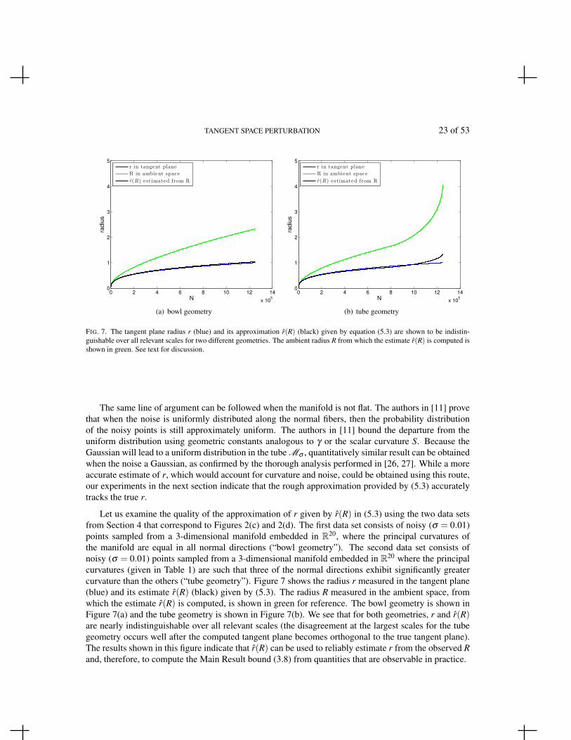
FIG. 7. The tangent plane radius r (blue) and its approximation r(R) (black) given by equation (5.3) are shown to be indistin-guishable over all relevant scales for two different geometries. The ambient radius R from which the estimate r(R) is computed isshown in green. See text for discussion.
The same line of argument can be followed when the manifold is not flat. The authors in [11] provethat when the noise is uniformly distributed along the normal fibers, then the probability distributionof the noisy points is still approximately uniform. The authors in [11] bound the departure from theuniform distribution using geometric constants analogous to γ or the scalar curvature S. Because theGaussian will lead to a uniform distribution in the tube Mσ , quantitatively similar result can be obtainedwhen the noise a Gaussian, as confirmed by the thorough analysis performed in [26, 27]. While a moreaccurate estimate of r, which would account for curvature and noise, could be obtained using this route,our experiments in the next section indicate that the rough approximation provided by (5.3) accuratelytracks the true r.
Let us examine the quality of the approximation of r given by r(R) in (5.3) using the two data setsfrom Section 4 that correspond to Figures 2(c) and 2(d). The first data set consists of noisy (σ = 0.01)points sampled from a 3-dimensional manifold embedded in R20, where the principal curvatures ofthe manifold are equal in all normal directions (“bowl geometry”). The second data set consists ofnoisy (σ = 0.01) points sampled from a 3-dimensional manifold embedded in R20 where the principalcurvatures (given in Table 1) are such that three of the normal directions exhibit significantly greatercurvature than the others (“tube geometry”). Figure 7 shows the radius r measured in the tangent plane(blue) and its estimate r(R) (black) given by (5.3). The radius R measured in the ambient space, fromwhich the estimate r(R) is computed, is shown in green for reference. The bowl geometry is shown inFigure 7(a) and the tube geometry is shown in Figure 7(b). We see that for both geometries, r and r(R)are nearly indistinguishable over all relevant scales (the disagreement at the largest scales for the tubegeometry occurs well after the computed tangent plane becomes orthogonal to the true tangent plane).The results shown in this figure indicate that r(R) can be used to reliably estimate r from the observed Rand, therefore, to compute the Main Result bound (3.8) from quantities that are observable in practice.
24 of 53 D. N. KASLOVSKY AND F. G. MEYER
5.2 Subspace Tracking and Recovery using the Ambient Radius
We now repeat the experiments of Section 4.1 by recomputing the subspace recovery error and subspacerecovery bounds using the radius in the ambient space, R, in place of the tangent plane radius, r. Wedemonstrate that, after converting the ambient radius R to its corresponding tangent plane radius r(R),the bound presented in the Main Result Theorem 3.1 accurately tracks the subspace recovery error.The presented results demonstrate that the Main Result may be used for tangent space recovery in thepractical setting where only the ambient radius is available.
We begin by generating 3-dimensional data sets embedded in R20 according to the specificationsgiven in Section 4.1. The curvature is chosen such that K = 12.6025 for all manifolds (excluding thelinear subspace example). The tube geometry is implemented by choosing principal curvatures as givenin Table 1 and the bowl geometry has all principal curvatures set to 1.0189. All but the noise-free dataset have Gaussian noise added with standard deviation σ = 0.01.
For each experiment, the ambient radius R is measured from the data and used to approximate thecorresponding tangent plane radius r(R) by equation (5.3), from which we compute our bound (3.8). Wethen compare this bound with the true subspace recovery error. Mimicking the experiments of Section4.1, the tangent plane at the local origin x0 is computed at each scale N via PCA of the N nearestneighbors of x0, where the distance from x0 (the radius R) is now measured in the ambient space RD.The true subspace recovery error ‖P− P‖F is then computed at each scale. The “true bound” is againcomputed by applying Theorem 2.1 after measuring each perturbation norm directly from the data. Werecall that this “true bound” requires no SVDs and utilizes information that is not practically availableto represent the best possible bound that we can hope to achieve. We will compare the mean of the trueerror and mean of the true bound over 10 trials (with error bars indicating one standard deviation) tothe bound given by our Main Result in Theorem 3.1, holding with probability greater than 0.8. We notethat for these experiments, the local origin x0 is given by oracle information and we will consider itsrecovery in a separate set of experiments.
The results are shown in Figure 8 and should be compared with those shown in Figure 2. Panel (a)shows the noisy curvature-free (linear subspace) result and we observe that the behaviors of the trueerror (blue), true bound (red), and main result bound (green) match the behaviors of their counterpartsin Figure 2(a) that were computed using r. In particular, the error in Figure 8(a) decays as 1/
√N (note
the logarithmic scale of the Y-axis). Our bound (green) accurately tracks the true error (blue) and isnearly indistinguishable from the true bound (red). Panel (b) shows the result for a noise-free manifoldwith tube geometry such that three of the normal directions exhibit high curvature while the others areflatter. We see that, much like in Figure 2(b), the main result bound (green) increases monotonically(ignoring the slight numerical instability at extremely small scales) to match the general behavior of thetrue error (blue) and true bound (red). Panel (c) shows the results for the noisy version of the manifoldused in panel (b). We observe that our bound (green) now exhibits blow up at small scales due to noiseand blow up at large scales due to curvature, matching the behavior of the true error. Finally, panel (d)shows the results for the noisy manifold with bowl geometry where all principal curvatures are equal,and indicates that our bound tracks the error at all scales. The dashed vertical lines in Figure 8 indicatethe locations of the minima of the true error curves (dashed blue) and the Main Result bounds (dashedgreen). We see that the location of the minimum of the Main Result bound is, in general, close to theminimum of the true error curve and falls within a range of scales for which the error is quite flat.
We observe that the results using R in Figure 8 are similar to those seen in Figure 2 using r, whilenoting that the true error for the tube geometry remains stable at larger scales in Figure 8 than the trueerror in Figure 2. To understand this observation, we examine the effect of geometry on the radii R and
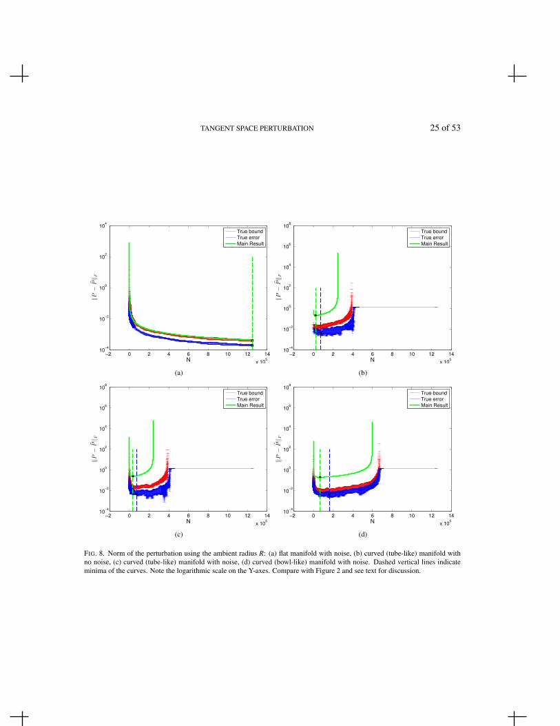
TANGENT SPACE PERTURBATION 25 of 53
−2 0 2 4 6 8 10 12 14
x 105
10−4
10−2
100
102
104
N
‖P
−P‖F
True bound
True error
Main Result
(a)
−2 0 2 4 6 8 10 12 14
x 105
10−4
10−2
100
102
104
106
108
N
‖P
−P‖F
True bound
True error
Main Result
(b)
−2 0 2 4 6 8 10 12 14
x 105
10−4
10−2
100
102
104
106
108
N
‖P
−P‖F
True bound
True error
Main Result
(c)
−2 0 2 4 6 8 10 12 14
x 105
10−4
10−2
100
102
104
106
108
N
‖P
−P‖F
True bound
True error
Main Result
(d)
FIG. 8. Norm of the perturbation using the ambient radius R: (a) flat manifold with noise, (b) curved (tube-like) manifold withno noise, (c) curved (tube-like) manifold with noise, (d) curved (bowl-like) manifold with noise. Dashed vertical lines indicateminima of the curves. Note the logarithmic scale on the Y-axes. Compare with Figure 2 and see text for discussion.
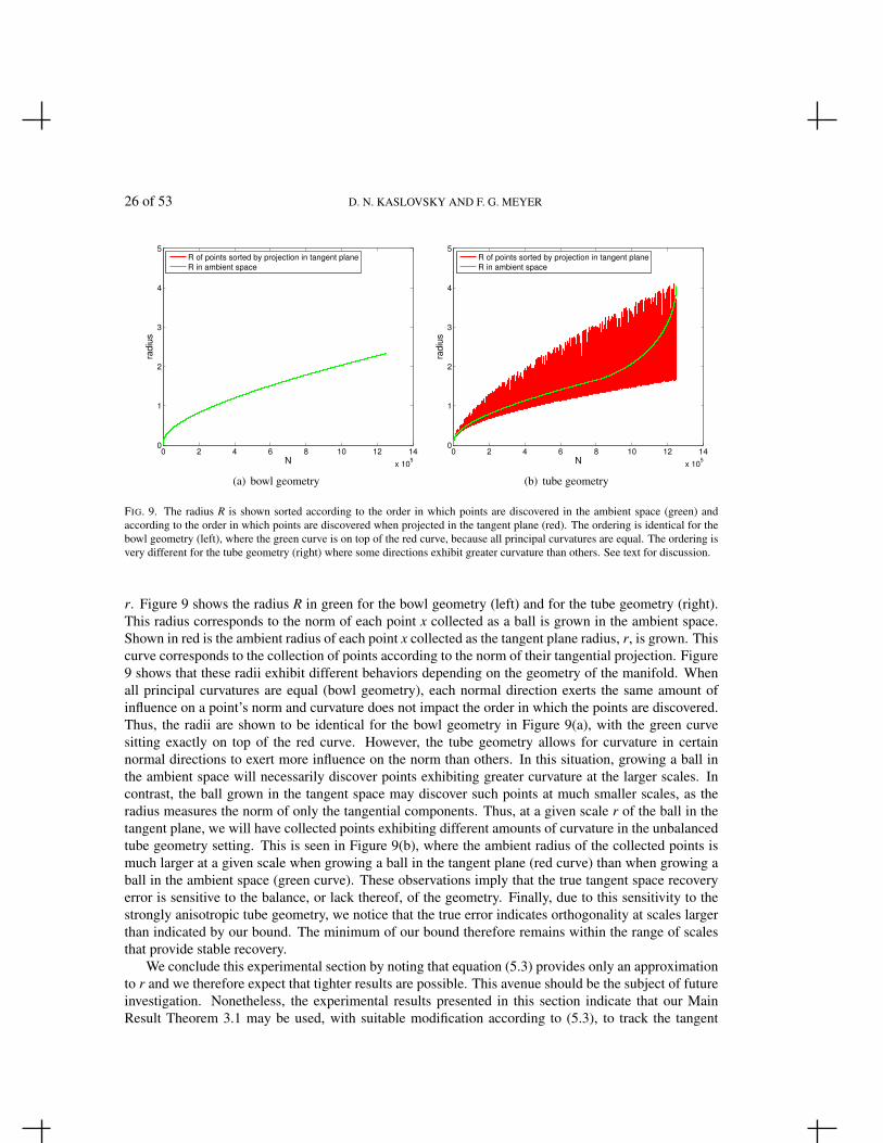
26 of 53 D. N. KASLOVSKY AND F. G. MEYER
0 2 4 6 8 10 12 14
x 105
0
1
2
3
4
5
N
radiu
s
R of points sorted by projection in tangent plane
R in ambient space
(a) bowl geometry
0 2 4 6 8 10 12 14
x 105
0
1
2
3
4
5
N
radiu
s
R of points sorted by projection in tangent plane
R in ambient space
(b) tube geometry
FIG. 9. The radius R is shown sorted according to the order in which points are discovered in the ambient space (green) andaccording to the order in which points are discovered when projected in the tangent plane (red). The ordering is identical for thebowl geometry (left), where the green curve is on top of the red curve, because all principal curvatures are equal. The ordering isvery different for the tube geometry (right) where some directions exhibit greater curvature than others. See text for discussion.
r. Figure 9 shows the radius R in green for the bowl geometry (left) and for the tube geometry (right).This radius corresponds to the norm of each point x collected as a ball is grown in the ambient space.Shown in red is the ambient radius of each point x collected as the tangent plane radius, r, is grown. Thiscurve corresponds to the collection of points according to the norm of their tangential projection. Figure9 shows that these radii exhibit different behaviors depending on the geometry of the manifold. Whenall principal curvatures are equal (bowl geometry), each normal direction exerts the same amount ofinfluence on a point’s norm and curvature does not impact the order in which the points are discovered.Thus, the radii are shown to be identical for the bowl geometry in Figure 9(a), with the green curvesitting exactly on top of the red curve. However, the tube geometry allows for curvature in certainnormal directions to exert more influence on the norm than others. In this situation, growing a ball inthe ambient space will necessarily discover points exhibiting greater curvature at the larger scales. Incontrast, the ball grown in the tangent space may discover such points at much smaller scales, as theradius measures the norm of only the tangential components. Thus, at a given scale r of the ball in thetangent plane, we will have collected points exhibiting different amounts of curvature in the unbalancedtube geometry setting. This is seen in Figure 9(b), where the ambient radius of the collected points ismuch larger at a given scale when growing a ball in the tangent plane (red curve) than when growing aball in the ambient space (green curve). These observations imply that the true tangent space recoveryerror is sensitive to the balance, or lack thereof, of the geometry. Finally, due to this sensitivity to thestrongly anisotropic tube geometry, we notice that the true error indicates orthogonality at scales largerthan indicated by our bound. The minimum of our bound therefore remains within the range of scalesthat provide stable recovery.
We conclude this experimental section by noting that equation (5.3) provides only an approximationto r and we therefore expect that tighter results are possible. This avenue should be the subject of futureinvestigation. Nonetheless, the experimental results presented in this section indicate that our MainResult Theorem 3.1 may be used, with suitable modification according to (5.3), to track the tangent
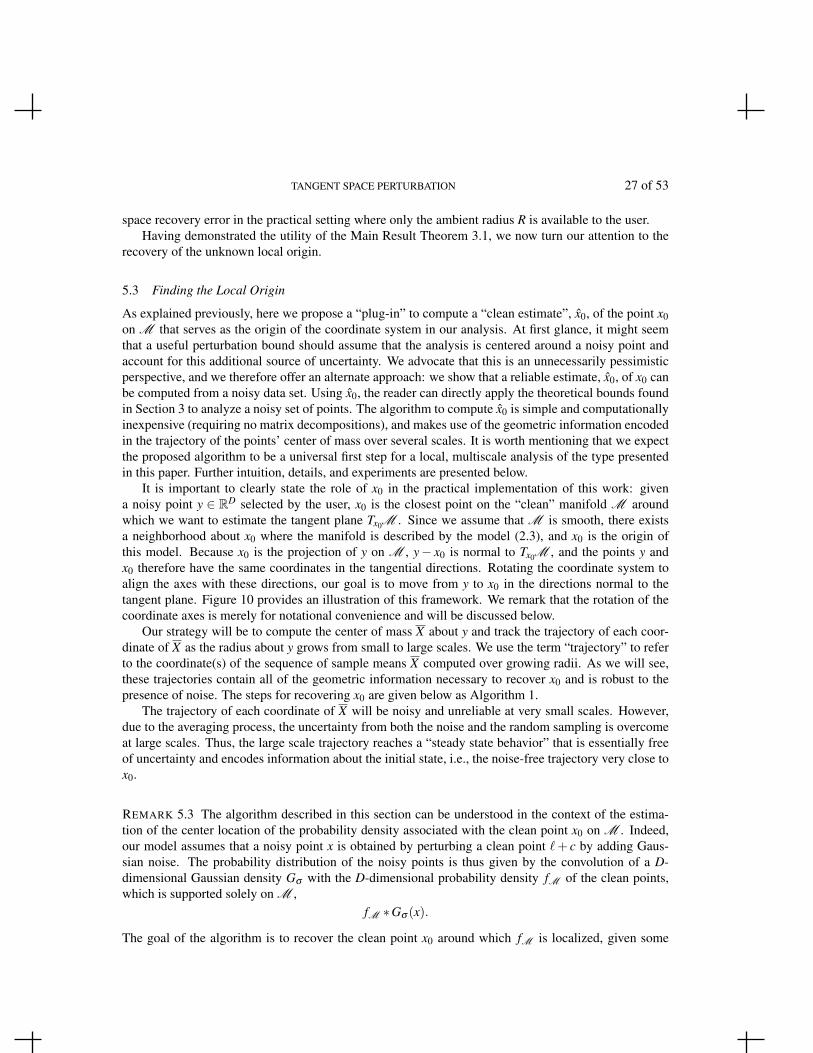
TANGENT SPACE PERTURBATION 27 of 53
space recovery error in the practical setting where only the ambient radius R is available to the user.Having demonstrated the utility of the Main Result Theorem 3.1, we now turn our attention to the
recovery of the unknown local origin.
5.3 Finding the Local Origin
As explained previously, here we propose a “plug-in” to compute a “clean estimate”, x0, of the point x0on M that serves as the origin of the coordinate system in our analysis. At first glance, it might seemthat a useful perturbation bound should assume that the analysis is centered around a noisy point andaccount for this additional source of uncertainty. We advocate that this is an unnecessarily pessimisticperspective, and we therefore offer an alternate approach: we show that a reliable estimate, x0, of x0 canbe computed from a noisy data set. Using x0, the reader can directly apply the theoretical bounds foundin Section 3 to analyze a noisy set of points. The algorithm to compute x0 is simple and computationallyinexpensive (requiring no matrix decompositions), and makes use of the geometric information encodedin the trajectory of the points’ center of mass over several scales. It is worth mentioning that we expectthe proposed algorithm to be a universal first step for a local, multiscale analysis of the type presentedin this paper. Further intuition, details, and experiments are presented below.
It is important to clearly state the role of x0 in the practical implementation of this work: givena noisy point y ∈ RD selected by the user, x0 is the closest point on the “clean” manifold M aroundwhich we want to estimate the tangent plane Tx0M . Since we assume that M is smooth, there existsa neighborhood about x0 where the manifold is described by the model (2.3), and x0 is the origin ofthis model. Because x0 is the projection of y on M , y− x0 is normal to Tx0M , and the points y andx0 therefore have the same coordinates in the tangential directions. Rotating the coordinate system toalign the axes with these directions, our goal is to move from y to x0 in the directions normal to thetangent plane. Figure 10 provides an illustration of this framework. We remark that the rotation of thecoordinate axes is merely for notational convenience and will be discussed below.
Our strategy will be to compute the center of mass X about y and track the trajectory of each coor-dinate of X as the radius about y grows from small to large scales. We use the term “trajectory” to referto the coordinate(s) of the sequence of sample means X computed over growing radii. As we will see,these trajectories contain all of the geometric information necessary to recover x0 and is robust to thepresence of noise. The steps for recovering x0 are given below as Algorithm 1.
The trajectory of each coordinate of X will be noisy and unreliable at very small scales. However,due to the averaging process, the uncertainty from both the noise and the random sampling is overcomeat large scales. Thus, the large scale trajectory reaches a “steady state behavior” that is essentially freeof uncertainty and encodes information about the initial state, i.e., the noise-free trajectory very close tox0.
REMARK 5.3 The algorithm described in this section can be understood in the context of the estima-tion of the center location of the probability density associated with the clean point x0 on M . Indeed,our model assumes that a noisy point x is obtained by perturbing a clean point `+ c by adding Gaus-sian noise. The probability distribution of the noisy points is thus given by the convolution of a D-dimensional Gaussian density Gσ with the D-dimensional probability density fM of the clean points,which is supported solely on M ,
fM ∗Gσ (x).
The goal of the algorithm is to recover the clean point x0 around which fM is localized, given some
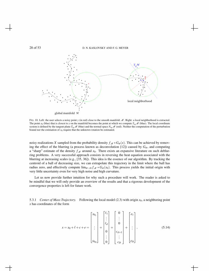
28 of 53 D. N. KASLOVSKY AND F. G. MEYER
local neighborhood
xT M
M
y
0
global manifold
x0
FIG. 10. Left: the user selects a noisy point y (in red) close to the smooth manifold M . Right: a local neighborhood is extracted.The point x0 (blue) that is closest to y on the manifold becomes the point at which we compute Tx0M (blue). The local coordinatesystem is defined by the tangent plane Tx0M (blue) and the normal space Nx0M (red). Neither the computation of the perturbationbound nor the estimation of x0 require that the unknown rotation be estimated.
noisy realizations X sampled from the probability density fM ∗Gσ (x). This can be achieved by remov-ing the effect of the blurring (a process known as deconvolution [12]) caused by Gσ , and computinga “sharp” estimate of the density fM around x0. There exists an expansive literature on such deblur-ring problems. A very successful approach consists in reversing the heat equation associated with theblurring at increasing scales (e.g., [35, 36]). This idea is the essence of our algorithm. By tracking thecentroid of a ball of decreasing size, we can extrapolate this trajectory in the limit where the ball hasradius zero, and effectively compute limσ→0 fM ∗Gσ (x0). This process yields the initial origin withvery little uncertainty even for very high noise and high curvature.
Let us now provide further intuition for why such a procedure will work. The reader is asked tobe mindful that we will only provide an overview of the results and that a rigorous development of theconvergence properties is left for future work.
5.3.1 Center of Mass Trajectory. Following the local model (2.3) with origin x0, a neighboring pointx has coordinates of the form
x = x0 + `+ c+ e =
x01
...
x0D
+
`1...`d
0...0
+
0...0
cd+1...
cD
+
e1
...
eD
, (5.14)
TANGENT SPACE PERTURBATION 29 of 53
Algorithm 1 Recovering the Local Origin x0
Input: Noisy points X = x(i)Ni=1, reference point y ∈ RD, scale intervals I (m)M
m=1 such that
I (m) = [R(m,1),R(m,2)] with R(m,1) < R(m,2) ∀m and
R(p,1) 6 R(q,1)
R(p,2) 6 R(q,2) for p > q
Outpt: Estimate x0 of the local origin x0 ∈M
FOR each scale interval I (m),m = 1, . . . ,M:
1. Center a ball at y and compute X = 1NB
∑NBi=1 x(i), the mean of the points inside the ball BD
y (Ry),∀Ry ∈I (m), where NB = |BD
y (Ry)|.
2. FOR each coordinate j = 1, . . . ,D:
(a) Fit (in the least squares sense) the trajectory of X j to the model
qy(Ry) = β2R2y +β0,
over the range of scales in I (m), explicitly requiring a zero first derivative at Ry = 0
(b) Set x(m)0 j
= β0
END
3. Set y = x(m)0
END
Return x0 = x(M)0 as the estimate of the local origin
and coordinate j of X is of the form
X j =1N
N
∑i=1
x(i)j =
x0 j +
1N ∑
Ni=1 `
(i)j + 1
N ∑Ni=1 e(i)j , j 6 d
x0 j +1N ∑
Ni=1 c(i)j + 1
N ∑Ni=1 e(i)j , j > d.
(5.15)
The sample mean X j =1N ∑
Ni=1 x(i)j approximates E[x j] with the uncertainty decaying as 1/
√N. More
precisely, by the Hoeffding inequality and the Gaussian tail bound, we have the following intervals forcoordinate j at scale N:
X j ∈
[x0 j −
√2ξ√N(r+σ), x0 j +
√2ξ√N(r+σ)
], j 6 d[(
x0 j +K jr2
2(d+2)
)−√
2ξ√N
(√dK(+)
j r2
2 +σ
),(
x0 j +K jr2
2(d+2)
)+√
2ξ√N
(√dK(+)
j r2
2 +σ
)], j > d
(5.16)with probability greater than 1−6e−ξ 2
. We see that while the coordinates exhibit variation about theirmeans at small scales, they reach their average (steady state) behavior with high probability at large
30 of 53 D. N. KASLOVSKY AND F. G. MEYER
scales. Thus, the large scale coordinate trajectories are controlled with little uncertainty for denselysampled data.
REMARK 5.4 More generally, we expect to observe data in a rotated coordinate system. Considerthe setting in R2 for a 1-dimensional manifold after applying a rotation to our conventional coordinatesystem. The observed coordinates will be of the form(
X1X2
)=
(x01x02
)+
(Q11 Q12Q21 Q22
)( 1N ∑
Ni=1 `
(i)1 + 1
N ∑Ni=1 e(i)1
1N ∑
Ni=1 c(i)2 + 1
N ∑Ni=1 e(i)2
)
=
x01 +Q11E[`]+Q12E[c]+ (Q11 +Q12)E[e]±O(
1√N
)x02 +Q21E[`]+Q22E[c]+ (Q21 +Q22)E[e]±O
(1√N
) (w.h.p.) (5.17)
=
x01 +Q12K2r2
2(d+2) ±O(
1√N
)x02 +Q22
K2r2
2(d+2) ±O(
1√N
),
where Q =
(Q11 Q12Q21 Q22
)is a unitary matrix. We see that all coordinates have the same form as coordinates
j > d in (5.16) with the slight modification introduced by the Qmn terms. In general, we will observea linear combination of all coordinates with weights Qmn < 1. In particular, all coordinates will be ofleading order r2 with a constant intercept (the origin), and all other orders of r appear as finite sampleuncertainty terms that decay as 1/
√N. Because an arbitrary rotation leaves all coordinates with the
same form as that of the coordinates j > d in equation (5.16), we proceed with the analysis of thesecoordinates without loss of generality.
Continuing from (5.16), we use a calculation similar to (5.1) to show that r2 ≈ R2 for small r. Wetherefore expect the coordinate trajectories ( j > d) to be quadratic functions of the observed radius Rwith intercept x0 and zero first derivative at R = 0. Fitting the observed trajectory of each coordinate tothe model
q(R) = β2R2 +β0 (5.18)
provides the least squares estimate of the origin x0 j = β0. By explicitly enforcing the zero first deriva-tive condition, the model (5.18) should be robust to uncertainty in the observed data at small scales.Moreover, initial estimates of x0 j may be obtained from the stable, large scale trajectories to anchor thesmall scale estimate using (5.18). We now examine this procedure in more detail.
5.3.2 Estimating x0. Equation (5.16) confirms our intuition that the large scale trajectory, smoothedfrom the averaging process, is very stable due to the 1/
√N decay of the finite sample uncertainty
terms. We must now cast this trajectory in terms of an observable radius Ry, the radius of a ball in RD
centered about the point y in the presence of noise. Recall that the intent of the following discussion isto informally derive the correct order for all terms, with complete rigor reserved for future work.
Consider first the effect of measuring the radius about a point other than x0. Let τ denote the offsetvector,
τ = y− x0 =[0 · · · 0 τd+1 · · · τD
]T,
since y and x0 only differ in their normal components. A calculation similar to (5.1) shows
R2y = ‖x− y‖2 = ‖x0 + `+ c− τ− x0‖2 = ‖`‖2 +‖c− τ‖2 6 r2 + γr4 +‖τ‖2. (5.19)
TANGENT SPACE PERTURBATION 31 of 53
Solving for r2 and injecting into (5.16) yields the following expression for X j (coordinates j > d) atscale N, holding with high probability:
X j ∈
[a1Ry +(x0 j −a0)−
√2ξ√N
a−1 , a1Ry +(x0 j −a0)+
√2ξ√N
a−1
], (5.20)
for Ry >
√‖τ‖2 +
14γ
, (5.21)
where
a1 =K j
2(d +2)√
γ, a0 =
K j
4(d +2)γ+O
(1Ry
), (5.22)
with uncertainty term
a−1 =12
√dγ
K(+)j Ry−
14
√d
γK(+)
j +O
(1Ry
). (5.23)
Next, reasoning in a manner similar to (5.1), we introduce the following correction for the presence ofthe noise, enlarging the radius Ry in (5.20) by σ
√D :
Ry← Ry +σ√
D.
We finally rewrite (5.20) to yield the expression for X j (coordinates j > d) at scale N, holding with highprobability:
X j ∈
[a1Ry +
(x0 j −a0 +a1σ
√D)−√
2ξ√N
a−1 , a1Ry +(
x0 j −a0 +a1σ√
D)+
√2ξ√N
a−1
], (5.24)
for Ry >
√‖τ‖2 +
14γ
,
with a1 and a0 as given by (5.22) and uncertainty term a−1 now taking the form
a−1 =12
√dγ
K(+)j Ry +
12
√dγ
K(+)j σ√
D− 14
√d
γK(+)
j +σ +O
(1Ry
). (5.25)
While (5.24) indicates that the large scale trajectory is linear in Ry, all of the necessary geometricinformation for Algorithm 1 to succeed is encoded in this trajectory. To see this, we proceed momen-tarily by taking a path slightly different from that of the proposed algorithm. Consider fitting the largescale trajectory to the model
qlineary (Ry) = α1Ry +α0 (5.26)
over the range of scale I (m) = [R(m,1)y ,R(m,2)
y ]. Let R(m,1)y correspond to N(m,1) points, R(m,2)
y correspond
to N(m,2) points, N(m,1) < N(m,2), and let N(m) = (N(m,1)+N(m,2))/2. The least squares fit of the largescale X j trajectory to (5.26) yields the coefficients
α1 ∈
[a1−
ξ√N(m)
√d2γ
K(+)j , a1 +
ξ√N(m)
√d2γ
K(+)j
](5.27)
32 of 53 D. N. KASLOVSKY AND F. G. MEYER
α0 ∈
[(x0 j −a0 +a1σ
√D)−√
2ξ√N(m)
(σ +
12
√dγ
K(+)j
(σ√
D− 12√
γ
)),
(x0 j −a0 +a1σ
√D)+
√2ξ√
N(m)
(σ +
12
√dγ
K(+)j
(σ√
D− 12√
γ
))]. (5.28)
Noting that the (rescaled) mean curvature K j is encoded in a1 and a0, we may recover a large scaleestimate of x0 j by setting
x(m)0 j
= α0−α1σ√
D+α21(d +2)
K j. (5.29)
Then we have
∣∣∣x0 j − x(m)0 j
∣∣∣ 6 √2ξ√
N(m)
(σ +
√d
2γK(+)
j
)+
ξ 2
N(m)
d(d +2)2γ
(K(+)j )2
|K j|, (5.30)
with high probability.
REMARK 5.5 The kth point of the X j trajectory has an uncertainty term that decays as 1/√
k. For
convenience, we have replaced the point-by-point uncertainty decay with a constant factor of 1/√
N(m)
above, where N(m) is the number of points in the middle of the current interval. A more rigorous analysiswould account for the heteroskedasticity of the sequence of sample means X j and use, e.g., a weightedleast squares fit to the model.
We may use these calculations to understand the initial large scale exploration performed by Algo-rithm 1. The estimate produced by the algorithm may be seen as the result of replacing the trajectorywith a linear function of Ry as given by (5.24). Then, discarding the data, we work only with this linearapproximation over all Ry. By doing so, we are discarding the quadratic behavior expected at smallscales near x0, as this part of the trajectory is damaged by the noise. We then recover the expectedquadratic behavior by fitting the linear approximation to the following quadratic model,
qquady (Ry) = β2R2
y +β0, (5.31)
where the zero first derivative condition is explicitly enforced. The estimate for coordinate j of x0 hasthe form
x0 j = α0 +α1F(I(m)), (5.32)
where
F(I (m)) =(R(m,2)
y )2 +4R(m,2)y R(m,1)
y +(R(m,1)y )2
6(R(m,2)y +R(m,1)
y )(5.33)
is a function of the scale interval. Comparing to (5.29), this estimate is equivalent to the previous largescale procedure when we choose
F(I (m)) =α1(d +2)
K j−σ√
D. (5.34)
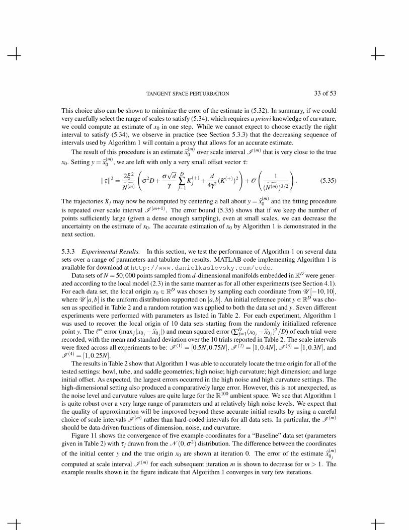
TANGENT SPACE PERTURBATION 33 of 53
This choice also can be shown to minimize the error of the estimate in (5.32). In summary, if we couldvery carefully select the range of scales to satisfy (5.34), which requires a priori knowledge of curvature,we could compute an estimate of x0 in one step. While we cannot expect to choose exactly the rightinterval to satisfy (5.34), we observe in practice (see Section 5.3.3) that the decreasing sequence ofintervals used by Algorithm 1 will contain a proxy that allows for an accurate estimate.
The result of this procedure is an estimate x(m)0 over scale interval I (m) that is very close to the true
x0. Setting y = x(m)0 , we are left with only a very small offset vector τ:
‖τ‖2 =2ξ 2
N(m)
(σ
2D+σ√
dγ
D
∑j=1
K(+)j +
d4γ2 (K
(+))2
)+O
(1
(N(m))3/2
). (5.35)
The trajectories X j may now be recomputed by centering a ball about y = x(m)0 and the fitting procedure
is repeated over scale interval I (m+1). The error bound (5.35) shows that if we keep the number ofpoints sufficiently large (given a dense enough sampling), even at small scales, we can decrease theuncertainty on the estimate of x0. The accurate estimation of x0 by Algorithm 1 is demonstrated in thenext section.
5.3.3 Experimental Results. In this section, we test the performance of Algorithm 1 on several datasets over a range of parameters and tabulate the results. MATLAB code implementing Algorithm 1 isavailable for download at http://www.danielkaslovsky.com/code.
Data sets of N = 50,000 points sampled from d-dimensional manifolds embedded inRD were gener-ated according to the local model (2.3) in the same manner as for all other experiments (see Section 4.1).For each data set, the local origin x0 ∈ RD was chosen by sampling each coordinate from U [−10,10],where U [a,b] is the uniform distribution supported on [a,b]. An initial reference point y ∈RD was cho-sen as specified in Table 2 and a random rotation was applied to both the data set and y. Seven differentexperiments were performed with parameters as listed in Table 2. For each experiment, Algorithm 1was used to recover the local origin of 10 data sets starting from the randomly initialized referencepoint y. The `∞ error (max j |x0 j − x0 j |) and mean squared error (∑D
j=1(x0 j − x0 j)2/D) of each trial were
recorded, with the mean and standard deviation over the 10 trials reported in Table 2. The scale intervalswere fixed across all experiments to be: I (1) = [0.5N,0.75N], I (2) = [1,0.4N], I (3) = [1,0.3N], andI (4) = [1,0.25N].
The results in Table 2 show that Algorithm 1 was able to accurately locate the true origin for all of thetested settings: bowl, tube, and saddle geometries; high noise; high curvature; high dimension; and largeinitial offset. As expected, the largest errors occurred in the high noise and high curvature settings. Thehigh-dimensional setting also produced a comparatively large error. However, this is not unexpected, asthe noise level and curvature values are quite large for the R100 ambient space. We see that Algorithm 1is quite robust over a very large range of parameters and at relatively high noise levels. We expect thatthe quality of approximation will be improved beyond these accurate initial results by using a carefulchoice of scale intervals I (m) rather than hard-coded intervals for all data sets. In particular, the I (m)
should be data-driven functions of dimension, noise, and curvature.Figure 11 shows the convergence of five example coordinates for a “Baseline” data set (parameters
given in Table 2) with τ j drawn from the N (0,σ2) distribution. The difference between the coordinatesof the initial center y and the true origin x0 are shown at iteration 0. The error of the estimate x(m)
0 j
computed at scale interval I (m) for each subsequent iteration m is shown to decrease for m > 1. Theexample results shown in the figure indicate that Algorithm 1 converges in very few iterations.
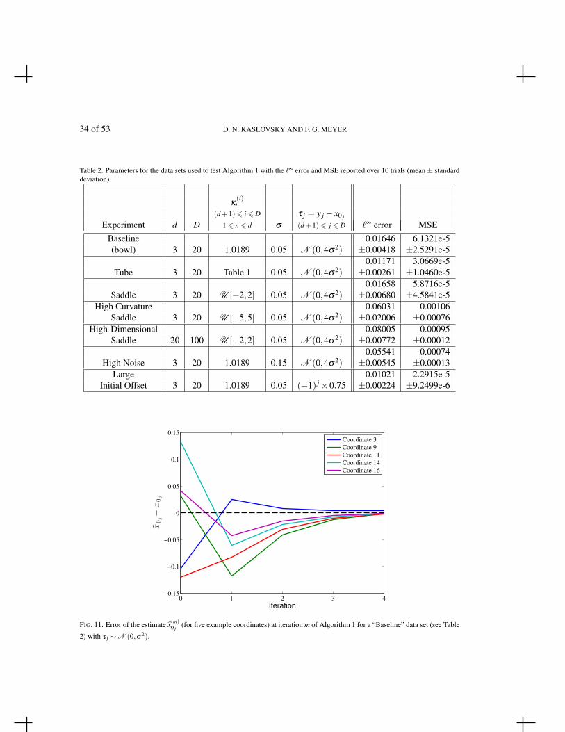
34 of 53 D. N. KASLOVSKY AND F. G. MEYER
Table 2. Parameters for the data sets used to test Algorithm 1 with the `∞ error and MSE reported over 10 trials (mean ± standarddeviation).
κ(i)n
(d +1)6 i6 D τ j = y j− x0 j
Experiment d D 16 n6 d σ (d +1)6 j 6 D `∞ error MSEBaseline 0.01646 6.1321e-5(bowl) 3 20 1.0189 0.05 N (0,4σ2) ±0.00418 ±2.5291e-5
0.01171 3.0669e-5Tube 3 20 Table 1 0.05 N (0,4σ2) ±0.00261 ±1.0460e-5
0.01658 5.8716e-5Saddle 3 20 U [−2,2] 0.05 N (0,4σ2) ±0.00680 ±4.5841e-5
High Curvature 0.06031 0.00106Saddle 3 20 U [−5,5] 0.05 N (0,4σ2) ±0.02006 ±0.00076
High-Dimensional 0.08005 0.00095Saddle 20 100 U [−2,2] 0.05 N (0,4σ2) ±0.00772 ±0.00012
0.05541 0.00074High Noise 3 20 1.0189 0.15 N (0,4σ2) ±0.00545 ±0.00013
Large 0.01021 2.2915e-5Initial Offset 3 20 1.0189 0.05 (−1) j×0.75 ±0.00224 ±9.2499e-6
0 1 2 3 4−0.15
−0.1
−0.05
0
0.05
0.1
0.15
Iteration
x0j−
x0j
Coordinate 3
Coordinate 9
Coordinate 11
Coordinate 14
Coordinate 16
FIG. 11. Error of the estimate x(m)0 j
(for five example coordinates) at iteration m of Algorithm 1 for a “Baseline” data set (see Table
2) with τ j ∼N (0,σ2).
TANGENT SPACE PERTURBATION 35 of 53
6. Discussion and Conclusion
6.1 Consistency with Previously Established Results
Local PCA of manifold-valued data has received attention in several recent works (for example, thosereferenced in Section 1). In particular, the analyses of [3] and [40], after suitable translation of notationand assumptions, demonstrate growth rates for the PCA spectrum that match those computed in thepresent work. The focus of our analysis is the perturbation of the eigenspace recovered from the localdata covariance matrix. We therefore confirm our results with those most similar from the literature. Themost closely related results are those of [31], in which matrix perturbation theory is used to study thePCA spectrum; [43], where neighborhood size and sampling conditions are given to ensure an accuratetangent space estimate from noise-free manifold-valued data; and [27], where theory is developed forthe implementation of multiscale PCA to detect the intrinsic dimension of a manifold.
In [31], a finite-sample PCA analysis assuming a linear model is presented. Keeping N and D fixed,the noise level σ is considered to be a small parameter. Much like the analysis of the present paper,the results are derived in the non-asymptotic setting. However, the bound on the angle between thefinite-sample and population eigenvectors is summarized in [31] for the asymptotic regime where N andD become large. The result, restated here in our notation, takes the form:
sinθU1,U1.
σ√λd
√DN+O(σ2).
We note that the main results of [31] are stated for N 6 D and that our analysis expects the oppositein general, although it is not explicitly required. Nonetheless, by setting curvature terms to zero, ourresults recover the reported leading behavior following the same asymptotic regime as [31], where termsO(1/
√N) are neglected and σ is treated as a small parameter. After setting all curvature terms to zero,
we assume condition 1 holds such that the denominator δ is sufficiently well conditioned and we maydrop all terms other than λd . Then our Main Result has the form:
sinθU1,U1.
1√N
1λd
σ√
d(D−d)[
r√d +2
+σ
]=
σ√λd
√d(D−d)√
N+O(σ2).
Setting d = 1 to match the analysis in [31] recovers its curvature-free result.Next, [43] presents an analysis of local PCA differing from ours in two crucial ways. First, the
analysis of [43] does not include high-dimensional noise perturbation and the data points are assumedto be sampled directly from the manifold. Second, the sampling density is not fixed, whereas the neigh-borhood size determines the number of sample points in our analysis. In fact, a goal of the analysis in[43] is to determine a sampling density that will yield an accurate tangent space estimate.
Allowing for a variable sampling density has the effect of decoupling the condition number δ−1
from the norm ‖UT2 ∆U1‖F measuring the amount of “lift” in directions normal to the tangent space
due to the perturbation. The analysis of [43] proceeds by first determining the optimal neighborhoodradius r∗ in the asymptotic limit of infinite sampling, N → ∞. This approach yields the requirementthat the spectra associated with the tangent space and curvature be sufficiently separated. Translating toour notation, setting noise terms to zero, and assuming the asymptotic regime of [43] such that we mayneglect finite-sample correction terms, we recover condition 1 of our Main Result Theorem 3.1:
λd−‖UT2 ∆U2‖F = λd−‖UT
21N
CCTU2‖F > 0. (6.1)
36 of 53 D. N. KASLOVSKY AND F. G. MEYER
Thus, Theorem 1 of [43] requires that r be chosen such that the subspace recovery problem is wellconditioned in the same sense that we require by condition 1. Substituting the expectations for eachterm in (6.1) yields
r2
(d +2)− K2r4(d +1)
2(d +2)2(d +4)> 0,
implying the choice r < c/K (for a constant c > 0), in agreement with the analysis of [43]. Once theproper neighborhood size has been selected, the decoupling assumed in [43] allows a choice of samplingdensity large enough to ensure a small angle. Again translating to our result (3.8), once r is selectedso that the denominator δ is well conditioned, the density may be chosen such that the 1/
√N decay of
the numerator ‖UT2 ∆U1‖F allows for a small recovery angle. Thus, we see that in the limit of infinite
sampling and absence of noise, our results are consistent with those of [43] in the fixed density setting.Finally, the recent work [27] studies multiscale PCA and the growth of the corresponding spectrum
to detect the intrinsic dimension of a manifold (or, more generally, a point cloud of random samples froma distribution concentrated around a low-dimensional manifold). The authors prove, under appropriateconditions, that the empirical covariance of noisy points localized in a Euclidean ball about a noisycenter is close to the population covariance of the underlying distribution, with high probability. Inparticular, the authors’ very detailed analysis shows that one may estimate the population covariancefrom the empirical covariance of noisy points that are localized before noise is added. Then, followingthe work in [26], further effort in [27] examines the effect of centering the multiscale analysis about anoisy origin.
Given an appropriate translation of the assumptions, the key results in [27] are of the same order asthose in the present work. Using our notation, [27] proceeds with an analysis of the geometric termscontained in the covariance 1
N X XT and bounds the difference from the population covariance by con-trolling the perturbation due to the noisy center and the localization process. In both the present analysisand that of [27], the empirical covariance 1
N X XT , computed from points localized before adding noise,provides the leading order terms that drive the behavior of ‖P− P‖F . By moving the analysis from r toR in Section 5, we allow both curvature and noise to affect the localization of points and experimentallyverify that ‖P− P‖F is consistent with our Main Result. Indeed, the results in Section 5 experimentallytest and confirm that the perturbation caused by such localization is small, as is theoretically derived in[27]. The effect of centering about a noisy origin is addressed in [27] through a rescaling of the observ-able radius, and conditions are given that allow for the covariance of the set of points localized abouta noisy origin to be close to the covariance of the points localized about the true origin. The algorithmintroduced in the present work, Algorithm 1 of Section 5, provides a simple method for recovering thetrue origin that may be used in practice. Through a very different framework than that of the analysisin [27], our method uses the geometric information encoded in the center of mass to compute the trueorigin of the local neighborhood. Our results therefore offer an algorithmic companion to the analysispresented in [27].
6.2 Algorithmic Considerations
6.2.1 Parameter Estimation. Practical methods must be developed to recover parameters such asdimension, curvature, and noise. Such parameters are necessary for any analysis or algorithm andshould be recovered directly from the data rather than estimated by a priori fixed values. The experi-mental results presented above suggest the particular importance of accurately estimating the intrinsicdimension d, for which there exist several algorithms. Fukunaga introduced a local PCA-based approachfor estimating d in [10]. The recent work in [3] presents a multiscale approach that estimates d in a
TANGENT SPACE PERTURBATION 37 of 53
pointwise fashion. Performing an SVD at each scale, d is determined by examining growth rate of themultiscale singular values. It would be interesting to investigate if this approach remains robust if onlya coarse exploration of the scales is performed, as it may be possible to reduce the computational costthrough an SVD-update scheme. Another scale-based approach is presented in [46] and the problemwas studied from a dynamical systems perspective in [9].
There exist statistical methods for estimating the noise level present in a data set that should beuseful in the context of this work (see, for example, [2, 5]). We experimentally obtain a reliable estimateof the noise level from the median of the smallest singular values over several small neighborhoods(results not shown). In [3], the smallest multiscale singular values are used as an estimate for the noiselevel and a scale-dependent estimate of noise variance is suggested in [7] for curve-denoising. Methodsfor estimating curvature (e.g., [23, 47]) have been developed for application to computer vision andextensions to the high-dimensional setting should be explored. Further, if one is willing to perform manySVDs of large matrices, our method of tracking the center of mass presented in Section 5 combined withthe growth rates for the PCA spectrum presented in [3] might yield the individual principal curvatures.
6.2.2 Sampling. For a tractable analysis, assumptions about sampling must be made. In this work wehave assumed uniform sampling in the tangent plane. This is merely one choice and we have conductedinitial experiments uniformly sampling the manifold rather than the tangent plane. Results suggestthat for a given radius, sampling the manifold yields a smaller curvature perturbation than that fromsampling the tangent plane. While more rigorous analysis and experimentation is needed, it is clear thatconsideration must be given to the sampling assumptions for any practical algorithm.
6.2.3 From Tangent Plane Recovery to Data Parameterization. The tangent plane recovered by ourapproach may not provide the best approximation over the entire neighborhood from which it wasderived. Depending on a user-defined error tolerance, a smaller or larger sized neighborhood may beparameterized by the local chart. If high accuracy is required, one might only parameterize a neighbor-hood of size N < N∗ to ensure the accuracy requirement is met. Similarly, if an application requiresonly modest accuracy, one may be able to parameterize a larger neighborhood than that given by N∗.
Finally, we may wish to use tangent planes recovered from different neighborhoods to construct acovering of a data set. There exist methods for aligning local charts into a global coordinate system (forexample [1, 37, 50], to name a few). Care should be taken to define neighborhoods such that a data setmay be optimally covered.
Funding
This work was supported by the National Science Foundation [DMS-0941476 to F.G.M. and D.N.K.,ACI-1226362 and DGE-0801680 to D.N.K.]; and the Department of Energy [DE-SC0004096 to F.G.M.].
Acknowledgements
The authors are grateful to the anonymous reviewers for their insightful comments and suggestions thatgreatly improved the content and presentation of this manuscript.
REFERENCES
[1] BRAND, M. (2003) Charting a Manifold. in Adv. Neural Inf. Process. Syst. 15, pp. 961–968. MIT Press.
38 of 53 D. N. KASLOVSKY AND F. G. MEYER
[2] BROOMHEAD, D. & KING, G. (1986) Extracting Qualitative Dynamics From Experimental Data. Phys. D,20(2-3), 217–236.
[3] CHEN, G., LITTLE, A., MAGGIONI, M. & ROSASCO, L. (2011) Some Recent Advances in Multiscale Geomet-ric Analysis of Point Clouds. in Wavelets and Multiscale Analysis: Theory and Applications, ed. by J. Cohen,& A. Zayed, pp. 199–225. Springer.
[4] DAVIS, C. & KAHAN, W. (1970) The Rotation of Eigenvectors by a Perturbation III. SIAM J. Numer. Anal., 7,1–46.
[5] DONOHO, D. & JOHNSTONE, I. (1995) Adapting to Unknown Smoothness via Wavelet Shrinkage. J. Amer.Statist. Assoc., 90, 1200–1224.
[6] EDELMAN, A. (1988) Eigenvalues and Condition Numbers of Random Matrices. SIAM J. Matrix Anal. Appl.,9(4), 543–560.
[7] FEISZLI, M. & JONES, P. (2011) Curve Denoising by Multiscale Singularity Detection and Geometric Shrink-age. Appl. Comput. Harmon. Anal., 31, 392–409.
[8] FEDERER, H. (1959) Curvature measures. Transactions of the American Mathematical Society, 93(3), 418–491.[9] FROEHLING, H., CRUTCHFIELD, J., FARMER, D., PACKARD, N. & SHAW, R. (1981) On Determining the
Dimension of Chaotic Flows. Phys. D, 3, 605–617.[10] FUKUNAGA, K. & OLSEN, D. (1971) An Algorithm for Finding Intrinsic Dimensionality of Data. IEEE Trans.
Comput., c-20(2), 176–183.[11] GENOVESE, C. R., PERONE-PACIFICO, M., VERDINELLI, I. & WASSERMAN, L. (2012) Minimax manifold
estimation. Journal of Machine Learning Research, 13, 1263–1291.[12] GENOVESE, C. R., PERONE-PACIFICO, M., VERDINELLI, I. & WASSERMAN, L. (2012a) Manifold estima-
tion and singular deconvolution under Hausdorff loss. The Annals of Statistics, 40(2), 941–963.[13] GIAQUINTA, M. & MODICA, G. (2009) Mathematical Analysis: An Introduction to Functions of Several
Variables. Springer.[14] GRAY, A. (1974) The volume of a small geodesic ball of a Riemannian manifold.. The Michigan Mathematical
Journal, 20(4), 329–344.[15] GOLUB, G. & LOAN, C. V. (1996) Matrix Computations. JHU Press.[16] JOHNSTONE, I. (2001) On the Distribution of the Largest Eigenvalue in Principal Component Analysis. Ann.
Statist., 29, 295–327.[17] JONES, P. (1990) Rectifiable sets and the Traveling Salesman Problem. Invent. Math., 102, 1–15.[18] JUNG, S. & MARRON, J. (2009) PCA Consistency in High Dimension, Low Sample Size Context. Ann. Statist.,
27, 4104–4130.[19] KAMBHATLA, N. & LEEN, T. (1997) Dimension Reduction by Local Principal Component Analysis. Neural
Comput., 9, 1493–1516.[20] KASLOVSKY, D. & MEYER, F. (2011) Image Manifolds: Processing Along the Tangent Plane. in 7th Interna-
tional Congress on Industrial and Applied Mathematics - ICIAM 2011.[21] (2011) Optimal Tangent Plane Recovery from Noisy Manifold Samples. http://arxiv.org/
abs/1111.4601v1.[22] (2012) Overcoming Noise, Avoiding Curvature: Optimal Scale Selection for Tangent Plane Recovery.
in Proc. IEEE Workshop on Statistical Signal Processing, pp. 904–907. http://dx.doi.org/10.1109/SSP.2012.6319851.
[23] KRSEK, P., LUKACS, G. & MARTIN, R. R. (1998) Algorithms for Computing Curvatures from Range Data.in The Mathematics of Surfaces VIII, Information Geometers, pp. 1–16.
[24] LAURANT, B. & MASSART, P. (2000) Adaptive Estimation of a Quadratic Functional by Model Selection.Ann. Statist., 28(5), 1302–1338.
[25] LIN, T. & ZHA, H. (2008) Riemannian Manifold Learning. IEEE Trans. Pattern Anal. Mach. Intell., 30, 796–809.
[26] LITTLE, A. V. (2011) Estimating the Intrinsic Dimension of High-Dimensional Data Sets: A Multiscale, Geo-
TANGENT SPACE PERTURBATION 39 of 53
metric Approach. Ph.D. thesis, Duke University.[27] LITTLE, A. V., MAGGIONI, M. & ROSASCO, L. (2012) Multiscale Geometric Methods for Data Sets I:
Multiscale SVD, Noise and Curvature. Discussion Paper MIT-CSAIL-TR-2012-029, Massachusetts Instituteof Technology.
[28] MEYER, F., KASLOVSKY, D. & WOHLBERG, B. (2012) Analysis of Image Patches: A Unified GeometricPerspective. SIAM Conference on Imaging Science (IS12).
[29] MITRA, N., NGUYEN, A. & GUIBAS, L. (2004) Estimating Surface Normals in Noisy Point Cloud Data.Internat. J. Comput. Geom. Appl., 14(4–5), 261–276.
[30] MUIRHEAD, R. (1982) Aspects of Multivariate Statistical Theory. Wiley.[31] NADLER, B. (2008) Finite Sample Approximation Results for Principal Component Analysis: A Matrix Per-
turbation Approach. Ann. Statist., 36, 2792–2817.[32] NIYOGI, P., SMALE, S. & WEINBERGER, S. (2011) A topological view of unsupervised learning from noisy
data. SIAM Journal on Computing, 40(3), 646–663.[33] OHTAKE, Y., BELYAEV, A. & SEIDEL, H.-P. (2006) A Composite Approach to Meshing Scattered Data.
Graph. Models, 68, 255–267.[34] ROWEIS, S. & SAUL, L. (2000) Nonlinear Dimensionality Reduction by Locally Linear Embedding. Science,
290, 2323–2326.[35] OSHER, S. & RUDIN, L. I. (1990) Feature-oriented image enhancement using shock filters. SIAM Journal on
Numerical Analysis, 27(4), 919–940.[36] PERONA, P. & MALIK, J. (1990) Scale-space and edge detection using anisotropic diffusion. Pattern Analysis
and Machine Intelligence, IEEE Transactions on, 12(7), 629–639.[37] ROWEIS, S., SAUL, L. & HINTON, G. (2002) Global Coordination of Locally Linear Models. in Adv. Neural
Inf. Process. Syst. 14, pp. 889–896. MIT Press.[38] RUDELSON, M. (1999) Random Vectors in the Isotropic Position. J. Funct. Anal., 164(1), 60–72.[39] SHAWE-TAYLOR, J. & CRISTIANINI, N. (2003) Estimating the Moments of a Random Vector with Applica-
tions. in Proc. of GRETSI 2003 Conference, pp. 47–52.[40] SINGER, A. & WU, H.-T. (2012) Vector Diffusion Maps and the Connection Laplacian. Comm. Pure Appl.
Math., 64, 1067–1144.[41] STEWART, G. & SUN, J. (1990) Matrix Perturbation Theory. Academic Press.[42] TROPP, J. (2011) User-Friendly Tail Bounds for Sums of Random Matrices. Found. Comput. Math., 12(4),
389–434.[43] TYAGI, H., VURAL, E. & FROSSARD, P. (2013) Tangent Space Estimation for Smooth Embeddings of
Riemannian Manifolds. Information and Inference, 2(1), 69–114.[44] VERSHYNIN, R. (2012) How Close is the Sample Covariance Matrix to the Actual Covariance Matrix. J.
Theoret. Probab., 25(3), 655–686.[45] VERSHYNIN, R. (2012) Introduction to the Non-Asymptotic Analysis of Random Matrices. in Compressed
Sensing, Theory and Applications, ed. by Y. Eldar, & G. Kutyniok, pp. 210–268. Cambridge.[46] WANG, X. & MARRON, J. (2008) A Scale-based Approach to Finding Effective Dimensionality in Manifold
Learning. Electron. J. Stat., 2, 127–148.[47] WILLIAMS, D. & SHAH, M. (1992) A Fast Algorithm for Active Contours and Curvature Estimation. Comput.
Vis. Image Und., 55(1), 14–26.[48] YANG, L. (2008) Alignment of Overlapping Locally Scaled Patches for Multidimensional Scaling and Dimen-
sionality Reduction. IEEE Trans. Pattern Anal. Mach. Intell., 30, 438–450.[49] ZHANG, T., SZLAM, A., WANG, Y. & LERMAN, G. (2010) Randomized Hybrid Linear Modeling by Local
Best-fit Flats. in CVPR, pp. 1927–1934.[50] ZHANG, Z. & ZHA, H. (2004) Principal Manifolds and Nonlinear Dimensionality Reduction via Tangent
Space Alignment. SIAM J. Sci. Comput., 26, 313–338.
40 of 53 D. N. KASLOVSKY AND F. G. MEYER
Appendix
Technical calculations are presented in this appendix. In particular, the norm of each random matrixcontributing to the perturbation term ∆ , defined in equation (2.15), is bounded with high probability.The analysis is divided between three cases: (1) norms of products of bounded random matrices; (2)norms of products of unbounded random matrices; and (3) norms of products of bounded and unboundedrandom matrices.
Each case requires careful attention to derive a tight result that avoids large union bounds and ensureshigh probability that is independent of the ambient dimension D. The analysis proceeds by boundingthe eigenvalues of the covariance matrices of (L−L), (C−C), and (E−E) using results from randommatrix theory and properties of the spectral norm. A detailed analysis of each of the three cases follows.
Before we start the proofs, one last comment is in order. The reader will notice that we sometimesintroduce benign assumptions about the number of samples N or the dimensions d or D in order toprovide bounds that are simpler to interpret. These assumptions are not needed to derive any of theresults; they are merely introduced to help us simplify a complicated expression, and introduce upperbounds that hold under these fairly benign assumptions. This should help the reader interpret the size ofthe different terms.
Notation
We often vectorize matrices by concatenating the columns of a matrix. If M = [m(1)| · · · |m(N)], then wedefine
−→m = vec(M) =
m(1)
...m(N)
.We denote the largest and smallest eigenvalue of a square matrix M by
λmax(M) and λmin(M),
respectively. In the main body of the paper, we use the standard notation X to denote the sample meanof N columns from the matrix X . In this appendix, we introduce a second notation to denote the sameconcept,
E[X ] = X =1N
N
∑n=1
x(n).
Finally, we denote by E[X ] the expectation of the random matrix X and by P[E] the probability of eventE.
A. Eigenvalue Bounds
A.1 Linear Eigenvalues
We seek a bound on the maximum and minimum (nonzero) eigenvalue of the matrix
1N(L−L)(L−L)T =
1N
N
∑k=1
(`(k)− `)(`(k)− `)T . (A.1)
TANGENT SPACE PERTURBATION 41 of 53
As only the nonzero eigenvalues are of interest, we proceed by considering only the nonzero upper-leftd×d block of the matrix in (A.1), or equivalently, by ignoring the trailing zeros of each realization `(k).Thus, momentarily abusing notation, we consider the matrix in (A.1) to be of dimension d× d. Theanalysis utilizes the following theorem found in [42].
THEOREM A.1 (Matrix Chernoff II, [42]) Consider a finite sequence Xk of independent, random, selfadjoint matrices that satisfy
Xk < 0 and λmax(Xk)6 λ∞ almost surely.
Compute the minimum and maximum eigenvalues of the sum of expectations,
µmin := λmin
(N
∑k=1E [Xk]
)and µmax := λmax
(N
∑k=1E [Xk]
).
Then
P
[λmin
(N
∑k=1
Xk
)6 (1−δ )µmin
]6 d
[e−δ
(1−δ )(1−δ )
]µmin/λ∞
, for δ ∈ [0,1], and
P
[λmax
(N
∑k=1
Xk
)> (1+δ )µmax
]6 d
[eδ
(1+δ )(1+δ )
]µmax/λ∞
, for δ > 0.
We apply this result to
Xk =1N(`(k)− `)(`(k)− `)T .
Clearly Xk is a symmetric positive semi-definite matrix and we have Xk < 0. Next,
λmax(Xk) =
∥∥∥∥ 1N(`(k)− `)(`(k)− `)T
∥∥∥∥2=
1N
∥∥∥`(k)− `∥∥∥26
1N
(‖`‖+‖`‖
)26
4r2
N
and we set λ∞ = 4r2/N. Simple computations yield
λmax
(N
∑k=1E[Xk]
)=
r2
d +2
[1− 1
N
]2
, and λmin
(N
∑k=1E[Xk]
)=
r2
d +2
[1− 1
N
]2
,
and we set
µmax = µmin = µ =r2
d +2
[1− 1
N
]2
.
By Theorem A.1 and using standard manipulations, we have the following result bound for the smallesteigenvalue, λd in our notation,
λd >r2
d +2
[1− 1
N
]2[
1−ξλd
1√N
√8(d +2)(1− 1
N )
]
with probability greater than 1−de−ξ 2
λd . Similarly, the following result holds for the largest eigenvalue,λ1 in our notation:
λ1 6r2
d +2
[1+ξλ1
5√
d +2√N
](A.2)
42 of 53 D. N. KASLOVSKY AND F. G. MEYER
with probability greater than 1−de−ξ 2
λ1 , as soon as N > 3. We define the last upper bound as
λbound(ξ ) =r2
d +2
[1+ξ
5√
d +2√N
], (A.3)
and we can use this bound to control the size of all the eigenvalues of the matrix 1N (L−L)(L−L)T ,
P` [λi 6 λbound(ξ ), i = 1, . . . ,d]> 1−de−ξ 2. (A.4)
Now that we have computed the necessary bounds for all nonzero linear eigenvalues, we return to ourstandard notation for the remainder of the analysis: each `(k) is of length D with `
(k)j = 0 for d+16 j6D
and L = [`(1)|`(2)| · · · |`(N)] is a D×N matrix.
A.2 Curvature Eigenvalues
To bound the largest eigenvalue, γ1, of 1N (C−C)(C−C)T we note that the spectral norm is bounded by
the Frobenius norm and we use the bound on the Frobenius norm derived in Section B.1. We can usethis bound to control the size of all the eigenvalues of the matrix 1
N (C−C)(C−C)T ,
P` [γi 6 γbound(ξ ), i = 1, . . . ,D−d]> 1−2e−ξ 2. (A.5)
where
γbound(ξ ) =r4
2(d +4)(d +2)2
√√√√ D
∑i, j=d+1
[(d +1)Ki jnn−Ki j
mn]2 +(K(+))2r4
4√
N
[(2+ξ
√2)+
(2+ξ√
2)2√
N
].
(A.6)The proof of the bound on the Frobenius norm is delayed until Section B.1.
REMARK A.1 A different (possibly tighter) bound may be derived using Theorem A.1. However, sucha bound would hold with a probability that becomes small when the ambient dimension D is large. Wetherefore proceed with the bound (A.6) above, noting that we sacrifice no additional probability by usingit here since it is required for the analysis in Section B.1.
A.3 Noise Eigenvalues
We may control the eigenvalues of 1N (E−E)(E−E)T using standard results from random matrix the-
ory. In particular, let smin(E) and smax(E) denote the smallest and largest singular value of matrix E,respectively. The following result (Corollary 5.35 of [45]) gives a tight control on the size of smin(E)and smax(E) when E has Gaussian entries.
THEOREM A.2 ([6, 45]) Let A be a D×N matrix whose entries are independent standard normal randomvariables. Then for every t > 0, with probability at least 1−2exp(−t2/2) one has
√N−√
D− t 6 smin(A) 6 smax(A) 6√
N +√
D+ t. (A.7)
TANGENT SPACE PERTURBATION 43 of 53
Define
α =
(σ
√1− 1
N
)−1
(A.8)
and note that the entries of Z = α(E −E) are independent standard normal random variables. Thisnormalization by α allows us to use Theorem A.2 and we divide by α2 to recover the result for (E−E)(E − E)T . Let us partition the Gaussian vector e into the first d coordinates, e1, and last D− dcoordinates, e2,
e =[e1 | e2
]T, (A.9)
and observe that the matrix UT1
1N (E−E)(E−ET
)U1 only depends on the realizations of e1. Similarly,the matrix UT
21N (E−E)(E−ET
)U2 only depends on the realizations of e2. By Theorem A.2, we have
λmax
(1N
UT1 (E−E)(E−ET
)U1
)6 σ
2(
1+5
2√
N(√
d +ξe1)
)(A.10)
with probability at least 1− e−ξ 2e1 over the random realization of e1, as soon as N > 4(
√d + ξe1), a
condition easily satisfied for any reasonable sampling density. Similarly,
λmax
(1N
UT2 (E−E)(E−ET
)U2
)6 σ
2(
1+5
2√
N(√
D−d +ξe2)
)(A.11)
with probability at least 1− e−ξ 2e2 over the random realization of e2, as soon as N > 4(
√D−d +ξe2).
B. Products of Bounded Random Matrices
B.1 Curvature Term: CCT
Begin by recalling the notation used for the curvature constants,
Ki =d
∑n=1
κ(i)n , K =
(D
∑i=d+1
K2i
) 12
, Ki jnn =
d
∑n=1
κ(i)n κ
( j)n , Ki j
mn =d
∑m,n=1m 6=n
κ(i)m κ
( j)n . (B.1)
The constant Ki quantifies the curvature in normal direction i, for i = (d + 1), . . . ,D. The overallcompounded curvature of the local model is quantified by K and is a natural result of our use of theFrobenius norm. We note that KiK j = Ki j
nn +Ki jmn. We also recall the positive constants
K(+)i =
(d
∑n=1|κ(i)
n |2) 1
2
, and K(+) =
(D
∑i=d+1
(K(+)i )2
) 12
. (B.2)
Our strategy for bounding the matrix norm ‖UT2
1N (C−C)(C−C)TU2‖F begins with the observation
that 1N (C−C)(C−C)T is a sample mean of N covariance matrices of the vectors (c(k)−c), k = 1, . . . ,N.
That is,1N(C−C)(C−C)T = E[(c− E[c])(c− E[c])T ]. (B.3)
44 of 53 D. N. KASLOVSKY AND F. G. MEYER
We therefore expect that 1N (C−C)(C−C)T converges toward the centered covariance matrix of c. We
will use the following result of Shawe-Taylor and Cristianini [39] to bound, with high probability, thenorm of the difference between this sample mean and its expectation.
THEOREM B.1 (Shawe-Taylor & Cristianini, [39]). Given N realizations of a random matrix Y dis-tributed with probability distribution PY , we have
PY
∥∥∥E[Y ]− E[Y ]∥∥∥F6
R√N
(2+ξ
√2)> 1− e−ξ 2
. (B.4)
The constant R = supsupp(PY )‖Y‖F , where supp(PY ) is the support of distribution PY .
We note that the original formulation of the result involves only random vectors, but since the Frobeniusnorm of a matrix is merely the Euclidean norm of its vectorized version, we formulate the theorem interms of matrices. We also note that the choice of R in (B.4) need not be unique. Our analysis willproceed by using upper bounds for ‖Y‖F which may not be suprema. Let
Rc = supc‖UT
2 c‖F .
Using Theorem B.1 and modifying slightly the proof of Corollary 6 in [39], which uses standard inequal-ities, we arrive at∣∣∣∣∥∥E[UT
2 (c−E[c])(c−E[c])TU2]∥∥
F −∥∥∥E[UT
2 (c− E[c])(c− E[c])TU2]∥∥∥
F
∣∣∣∣6∥∥∥E[UT
2 ccTU2]− E[UT2 ccTU2]
∥∥∥F+∥∥∥E[UT
2 c]− E[UT2 c]∥∥∥2
F6
R2c√N
(2+ξc
√2)+
R2c
N
(2+ξc
√2)2
with probability greater than 1−2e−ξ 2c over the random selection of the sample points. To complete the
bound we must compute Rc and∥∥E[UT
2 (c−E[c])(c−E[c])TU2]∥∥
F . A simple norm calculation shows
‖UT2 c‖2
F =14
D
∑i=d+1
(κ(i)1 `2
1 + . . . +κ(i)d `2
d
)26
r4
4
D
∑i=d+1
(K(+)
i
)2=
(K(+))2r4
4,
and we set Rc = K(+)r2/2. Next, the expectation takes the form∥∥∥E[UT2 (c−E[c])(c−E[c])TU2]
∥∥∥F
=∥∥∥E[UT
2 ccTU2]−E[UT2 c]E[cTU2]
∥∥∥F.
We calculate
E[cic j] =
[3Ki j
nn +Ki jmn
]r4
4(d +2)(d +4), and E[ci]E[c j] =
[Ki j
nn +Ki jmn
]r4
4(d +2)2
and compute the norm
∥∥∥E[UT2 (c−E[c])(c−E[c])TU2]
∥∥∥F=
r4
2(d +2)2(d +4)
√√√√ D
∑i, j=d+1
[(d +1)Ki j
nn−Ki jmn
]2.
TANGENT SPACE PERTURBATION 45 of 53
Finally, putting it all together, we conclude that
∥∥∥∥UT2
1N(C−C)(C−C)TU2
∥∥∥∥F6
r4
2(d +2)2(d +4)
√√√√ D
∑i, j=d+1
[(d +1)Ki j
nn−Ki jmn
]2
+1√N(K(+))2r4
4
[(2+ξc
√2)+
1√N
(2+ξc
√2)2]
with probability greater than 1−2e−ξ 2c over the random selection of the sample points.
B.2 Curvature-Linear Cross-Terms: CLT
Our approach for bounding the matrix norm ‖UT2
1N (C−C)(L−L)TU1‖F mirrors that of Section B.1.
Here, we use that E[`i] = 0 for 16 i6 d and proceed as follows. We have
R` = sup`‖`TU1‖F = r.
Reasoning as in the previous section, we have∣∣∣∣∥∥E[UT2 (c−E[c])(`−E[`])TU1]
∥∥F −
∥∥∥E[UT2 (c− E[c])(`− E[`])TU1]
∥∥∥F
∣∣∣∣6∥∥∥E[UT
2 c`TU1]− E[UT2 c`TU1]
∥∥∥F+∥∥∥E[`TU1]−E[`TU1]
∥∥∥F
(∥∥∥E[UT2 c]−E[UT
2 c]∥∥∥
F+∥∥E[UT
2 c]∥∥
F
)6
RcR`√N
(2+ξc`
√2)+
R`√N
(2+ξ`
√2)[ Rc√
N
(2+ξc
√2)+∥∥E[UT
2 c]∥∥
F
]with probability greater than 1− e−ξ 2
c` − e−ξ 2` − e−ξ 2
c over the random selection of the sample points.Finally, we set ξ` = ξc` and conclude∥∥∥∥UT
21N(C−C)(L−L)TU1
∥∥∥∥F6
K(+)r3
2√
N
[d +3d +2
(2+ξc`
√2)+
1√N
(2+ξc
√2)(
2+ξc`√
2)]
with probability greater than 1−2e−ξ 2c` − e−ξ 2
c over the random selection of the sample points.
C. Products of Unbounded Random Matrices: EET
We seek bounds for the matrix norms of the form∥∥∥∥UTn
1N(E−E)(E−E)TUm
∥∥∥∥F
for (n,m) = (1,1),(2,2), and (2,1). (C.1)
Because E is composed of N columns of independent realizations of a D-dimensional Gaussian vector,the matrix A defined by
A =1
N−11
σ2 (E−E)(E−E)T =α2
N(E−E)(E−E)T
46 of 53 D. N. KASLOVSKY AND F. G. MEYER
is Wishart WD(N−1, 1
N−1 ID), where α =
(σ
√1− 1
N
)−1
. As a result, we can quickly compute bounds
on the terms (C.1) since they can be expressed as the norm of blocks of A. Indeed, let us partition A asfollows
A =
[A11 A12A21 A22
],
where A11 is d×d, A22 is (D−d)×(D−d). We now observe that Anm is not equal to α2
N UTn (E−E)(E−
E)TUm, but both matrices have the same Frobenius norm. Precisely, the two matrices differ only by aleft and a right rotation, as explained in the next few lines.
Since only the first d entries of each column in U1 are nonzero, we can define two matrices P1 andQ1 that extract the first d entries and apply the rotation associated with U1, respectively, as follows
U1 =
Q1
0 0...
...0 0
=
1 0
0 10 0...
...0 0
Q1 = P1Q1.
We define similar matrices P2 and Q2 such that U2 = P2Q2. We conclude that
∥∥UTn (E−E)(E−E)TUm
∥∥F =
∥∥PTn (E−E)(E−E)T Pm
∥∥F =
Nα2 ‖Anm‖F .
In summary, we can control the size of the norms (C.1) by controlling the norm of the sub-matrices of aWishart matrix. We first estimate the size of ‖A11‖F and ‖A22‖F . This is a straightforward affair, sincewe can apply Theorem A.2 with P1(E−E) and P2(E−E), respectively, to get the spectral norm of A11and A22. We then apply a standard inequality between the spectral and the Frobenius norm of a matrixM,
‖M‖F 6√
rank(M)‖M‖2. (C.2)
This bound is usually quite loose and equality is achieved only for the case where all singular values ofmatrix A are equal. It turns out that this special case holds in expectation for the matrices in the analysisto follow, and thus (C.2) provides a tight estimate of the Frobenius norm. Using (A.10) and (C.2), wehave the following bound∥∥∥∥UT
11N(E−E)(E−E)TU1
∥∥∥∥F6 σ
2√
d[
1+52
1√N(√
d +ξe1
√2)]
with probability greater than 1−e−ξ 2e1 over the random realization of the noise. By (A.11), we also have∥∥∥∥UT
21N(E−E)(E−E)TU2
∥∥∥∥F6 σ
2√D−d[
1+52
1√N(√
D−d +ξe2
√2)]
with probability greater than 1− e−ξ 2e2 over the random realization of the noise.
TANGENT SPACE PERTURBATION 47 of 53
It remains to bound ‖A21‖. Here we proceed by conditioning on the realization of the last D− dcoordinates of the noise vectors in the matrix E; in other words, we freeze P2E. Rather than workingwith Gaussian matrices, we prefer to vectorize the matrix A21 and define
−→a21 = vec(AT
21).
Note that here we unroll the matrix A21 row by row to build −→a21. Because the Frobenius norm of A21is the Euclidean norm of −→a21, we need to find a bound on ‖−→a21‖. Conditioning on the realization ofP2E, we know (Theorem 3.2.10 of [30]) that the distribution of −→a21 is a multivariate Gaussian variableN (−→0 ,S), where
−→0 is the zero vector of dimension d(D− d) and S is the d(D− d)× d(D− d) block
diagonal matrix containing d copies of 1N A22
S =1N
A22
A22. . .
A22
.Let S† be a generalized inverse of S (such that SS†S = S), then (see e.g. Theorem 1.4.4 of [30])
−→a21T S†−→a21 ∼ χ
2(rank(S)).
Now, using only the bound for the smallest singular value in Theorem A.2, A22 has full rank, (D−d),with probability 1−e−(
√N−√
D−d)2/2, and therefore S has full rank, d(D−d), with the same probability.In the following, we derive an upper bound on the size of ‖−→a21‖ when A22 has full rank. A similar – buttighter – bound can be derived when S is rank deficient; we only need to replace (D−d) by the rank ofA22 in the bound that follows. Because the bound derived when A22 is full rank will hold when A22 isrank deficient (an event which happens with very small probability, anyway), we only worry about thiscase in the following. In this case, S† = S−1 and
−→a21T S−1−→a21 ∼ χ
2(d(D−d)).
Finally, using a corollary of Laurant and Massart (immediately following Lemma 1 of [24]), we get that,−→a21
T S−1−→a21 6 d(D−d)+2ξe3
√d(D−d)+2ξ
2e3
(C.3)
with probability greater than 1− e−ξ 2e3 . In the following, we assume that ξe3 6 0.7
√d(D−d), which
happens as soon as d or D have a moderate size. Under this mild assumption we have√d(D−d)+2ξe3
√d(D−d)+2ξ 2
e36√
d(D−d)
(1+
65
ξe3√d(D−d)
).
In order to compare ‖−→a21‖2 to −→a21T S−1−→a21, we compute the eigendecomposition of S,
S = O Π OT ,
where O is a unitary matrix and Π contains the eigenvalues of 1N A22, repeated d times. Letting
λmax( 1
N A22)
be the largest eigenvalue of 1N A22, we get the following upper bound,
‖−→a21‖2 6 λmax
(1N
A22
)−→a21
T OTΠ−1O−→a21 = λmax
(1N
A22
)−→a21
T S−1−→a21.
48 of 53 D. N. KASLOVSKY AND F. G. MEYER
We conclude that, conditioned on a realization of the last D−d entries of E, we have
Pe1
‖−→a21‖6
√λmax
(1N
A22
)√d(D−d)
[1+
65
ξe3√d(D−d)
]|e2
> 1− e−ξ 2
e3 . (C.4)
To derive a bound on ‖−→a21‖ that holds with high probability, we consider the event
Eε,ξ =
‖−→a21‖6
√d(D−d)√
N
(1+√
D−d + ε√N
)[1+
65
ξ√d(D−d)
].
As we will see in the following, the event Eε,ξ happens with high probability. This event depends onthe random realization of the top d coordinates, e1, of the Gaussian vector e (see (A.9)). Let us define asecond likely event, which depends only on e2 (the last D−d coordinates of e),
Ee2 =
√λmax
(1N
A22
)6
1√N
(1+√
D−d + ε√N
).
Theorem A.2 tells us that the event Ee2 is very likely, and Pe2 (Ece2) 6 e−ε2/2. We now show that the
probability of Ecε,ξ is also very small,
Pe1,e2(Ecε,ξ ) = Pe1,e2(E
cε,ξ ∩Ee2)+Pe1,e2(E
cε,ξ ∩E
ce2)6 Pe1,e2(E
cε,ξ ∩Ee2)+Pe2(E
ce2).
In order to bound the first term, we condition on e2,
Pe1,e2(Ecε,ξ ∩Ee2) = Ee2
[Pe1(E
cε,ξ ∩Ee2 |e2)
].
Now the two conditions,‖−→a21‖>
√d(D−d) 1√
N
(1+
√D−d+ε√
N
)[1+ 6
5ξ√
d(D−d)
]1√N
(1+
√D−d+ε√
N
)>√
λmax( 1
N A22)
imply that
‖−→a21‖>√
d(D−d)
√λmax
(1N
A22
)[1+
65
ξ√d(D−d)
],
and thus
Pe1(Ecε,ξ ∩Ee2 |e2)6 Pe1
(‖−→a21‖>
√d(D−d)
√λmax
(1N
A22
)[1+
65
ξ√d(D−d)
]|e2
).
Because of (C.4) the probability on the right-hand side is less than e−ξ 2, which does not depend on e2.
We conclude thatPe1,e2(E
cε,ξ )6 e−ε2/2 + e−ξ 2
.
TANGENT SPACE PERTURBATION 49 of 53
Finally, since∥∥∥∥UT2
1N(E−E)(E−E)TU1
∥∥∥∥F= σ
2(
1− 1N
)‖A21‖F = σ
2(
1− 1N
)‖−→a21‖,
we have∥∥∥∥ 1N
UT2 (E−E)(E−E)TU1
∥∥∥∥F6
σ2√
d(D−d)√N
(1+√
D−d +ξe2
√2√
N
)[1+
65
ξe3√d(D−d)
]
with probability greater than 1− e−ξ 2e2 − e−ξ 2
e3 over the realization of the noise.
D. Products of Bounded and Unbounded Random Matrices
D.1 Linear-Noise Cross-Terms: ELT
Our goal is to bound the matrix norm 1N ‖U
Tm (E−E)(L−L)TU1‖F , with high probability, for m= 1,2.
We detail the analysis for the case where m = 1 and note that the analysis for m = 2 is identical up tothe difference in dimension. Using the decomposition of the matrix U1 = P1Q1 defined in the previoussection, we have
1N
∥∥UT1 (E−E)(L−L)TU1
∥∥F =
1N
∥∥PT1 (E−E)(L−L)T P1
∥∥F . (D.1)
Before proceeding with a detailed analysis of this term, let us derive a bound, which will prove to bevery precise, using a back of the envelope analysis. The entry (i, j) in the matrix 1
N PT1 (E−E)(L−L)T P1
is given by1N
N
∑k=1
(e(k)i − ei)(`(k)j − ` j),
and it measures the average correlation between coordinate i6 d of the (centered) noise term and coor-dinate j 6 d of the linear tangent term. Clearly, this empirical correlation has zero mean, and an upperbound on its variance is given by
1N
σ2λ1,
where the top eigenvalue λ1 measures the largest variance of the random variable `, measured along thefirst column of U1. Since the matrix PT
1 (E−E)(L−L)T P1 is d×d, we expect
1N
∥∥PT1 (E−E)(L−L)T P1
∥∥F ≈
1√N
σ
√λ1d.
We now proceed with the rigorous analysis. The singular value decomposition of PT1 (L−L) is given by
PT1 (L−L) = Q1ΣV T , (D.2)
where Σ is the d×d matrix of the singular values, and V is a matrix composed of d orthonormal columnvectors of size N. Injecting the SVD of PT
1 (L−L) we have
1N
∥∥PT1 (E−E)(L−L)T P1
∥∥F =
1N
∥∥PT1 (E−E)V ΣQT
1∥∥
F =1N
∥∥PT1 (E−E)V Σ
∥∥F
6
√λ1√N
∥∥PT1 (E−E)V
∥∥F . (D.3)
50 of 53 D. N. KASLOVSKY AND F. G. MEYER
DefineZ1 = αPT
1 (E−E)V.
Each row of Z1 is formed by the projections of the corresponding row of αPT1 (E − E) onto the d-
dimensional subspace of RN formed by the columns of V . As such, the projected row is a d-dimensionalGaussian vector, the norm of which scales like
√d with high probability.
The only technical difficulty involves the fact that the columns of V change with the different real-izations of L. We need to check that this random rotation of the vectors in V does not affect the sizeof the norm of Z1. Proceeding in two steps, we first freeze a realization of L, and compute a bound on∥∥PT
1 (E−E)V∥∥
F that does not depend on L. We then remove the conditioning on L, and compute theprobability that ‖Z1‖F is very close to d.
Instead of working with Z1, we define the d2-dimensional vector
−→z1 = vec(ZT
1).
Consider the Nd-dimensional Gaussian vector
−→g1 = α vec(PT
1 (E−E))∼N (0, INd).
In the next few lines, we construct an orthogonal projector P such that~z1 = P~g1. As a result, we willhave that −→z1 ∼N (0, Id2), and using standard results on the concentration of the Gaussian measure, wewill get an estimate of ‖PT
1 (E−E)V‖F = α−1‖~z1‖.
First, consider the following d2×Nd matrix
V=
V T
V T
. . .V T
,formed by stacking d copies of V T in a block diagonal fashion with no overlap (note that V T is nota square matrix). We observe that because no overlap exists between the blocks, the rows of V areorthonormal and V is an orthogonal projector from RNd to Rd2
.Now, we consider the Nd×Nd permutation matrix Ω constructed as follows. We first construct the
d×Nd matrix Ω1 by interleaving blocks of zeros of size d× (N− 1) between the columns vectors ofthe d×d identity matrix,
Ω1 =
∣∣∣∣∣∣∣∣∣10...0
∣∣∣∣∣∣∣∣∣0 · · · 00 · · · 0...0 · · · 0
∣∣∣∣∣∣∣∣∣01...0
∣∣∣∣∣∣∣∣∣0 · · · 00 · · · 0...0 · · · 0
· · ·
∣∣∣∣∣∣∣∣∣00...1
∣∣∣∣∣∣∣∣∣0 · · · 00 · · · 0...0 · · · 0
.Now consider the matrix Ω2 obtained by performing a circular shift of the columns Ω1 to the right byone index,
Ω2 =
00...0
∣∣∣∣∣∣∣∣∣10...0
∣∣∣∣∣∣∣∣∣0 · · · 00 · · · 0
...0 · · · 0
∣∣∣∣∣∣∣∣∣01...0
∣∣∣∣∣∣∣∣∣0 · · · 00 · · · 0...0 · · · 0
· · ·
00...0
∣∣∣∣∣∣∣∣∣00...1
∣∣∣∣∣∣∣∣∣0 · · ·0 · · ·...0 · · ·
.
TANGENT SPACE PERTURBATION 51 of 53
We can iterate this process N− 1 times and construct N such matrices, Ω1, . . . ,ΩN . Finally, we stackthese N matrices to construct the Nd×Nd permutation matrix
Ω =
Ω1...
ΩN
.By construction, Ω only contains a single nonzero entry, equal to one, in every row and every column,and therefore is a permutation matrix. Finally, the matrix Ω allows to move the action of V from theright of E to the left, and we have
−→z1 = VΩ−→g1 . (D.4)
Putting everything together, we conclude that the matrix defined by
P= VΩ (D.5)
is an orthogonal projector, and therefore −→z1 ∼N (0, Id2). Using again the previous bound (C.3) on thenorm of a Gaussian vector, we have
Pe
(‖−→z1‖6
(d +
65
ε
)|L)> 1− e−ε2
. (D.6)
To conclude the proof, we remove the conditioning on L, and using (D.6) we have
Pe,`
(‖−→z1‖6
(d +
65
ε
))= E`Pe
(‖−→z1‖6
(d +
65
ε
)|L)> 1− e−ε2
.
Since ‖PT1 (E−E)V‖F = α−1‖−→z1‖, we have
Pe,`
(‖PT
1 (E−E)V‖F 6 σ
√1− 1
N
(d +
65
ε
))> 1− e−ε2
. (D.7)
Finally, combining (A.3), (A.4), (D.1), (D.3), and (D.7) we conclude that
Pe,`
(1N
∥∥UT1 (E−E)(L−L)TU1
∥∥F 6
σ√
λbound(ξ )√N
√1− 1
N
(d +
65
ε
))> (1− e−ε2
)(1−de−ξ 2) (D.8)
which implies
Pe,`
(1N
∥∥UT1 (E−E)(L−L)TU1
∥∥F 6
σ r√N√
d +2
[1+ξ
5√
d +2√N
](d +
65
ε
))> (1− e−ε2/2)(1−de−ξ 2
).
A similar bound holds for∥∥UT
21N (E−E)(L−L)TU1
∥∥F . Indeed, we define
Z2 = αPT2 (E−E)V, −→z2 = vec(Z2) , and −→g2 = α vec
(PT
2 (E−E)). (D.9)
52 of 53 LIST OF FIGURES
Again, we can construct an orthogonal projector P′ with size d(D−d)×N(D−d) so that−→z2 = P′−→g2 . (D.10)
By combining (D.4) and (D.10), we can control the concatenated vector[−→z1
−→z2]T by estimating the
norm of[−→g1
−→g2]T . We conclude that
‖UT1
1N (E−E)(L−L)TU1‖F
‖UT2
1N (E−E)(L−L)TU1‖F
6 σ r√N√
d +2
[1+ξλ1
5√
d +2√N
]d + 6
5 ξe`√d(D−d) + 6
5 ξe`
(D.11)
with probability greater than (1−de−ξ 2
λ1 )(1−e−ξ 2e`) over the joint random selection of the sample points
and random realization of the noise.
D.2 Curvature-Noise Cross-Terms: CET
The analysis to bound the matrix norm
1N
∥∥UT2 (C−C)(E−E)TUm
∥∥F =
1N
∥∥UTm (E−E)(C−C)TU2
∥∥F
for m = 1,2 proceeds in an identical manner to that for the bound on ‖ 1N UT
m (E −E)(L−L)TU1‖F .We therefore give only a brief outline here. Mimicking the reasoning that leads to (D.8), we get
Pe,`
(1N
∥∥UT1 (E−E)(C−C)TU2
∥∥F 6
σ√
γbound(ξ )√N
√1− 1
N
(√d(D−d)+
65
ε
))> (1− e−ε2
)(1−de−ξ 2),
where γbound(ξ ) is the bound on all the eigenvalues of 1N UT
2 (C−C)(C−C)TU2 defined in (A.6). Thisleads to a bound similar to (D.11) for the tangential and curvature components of the noise,
‖UT2
1N (C−C)(E−E)TU1‖F
‖UT2
1N (C−C)(E−E)TU2‖F
6 σ√
γbound(ξc)√N
√
d(D−d) + 65 ξce
(D−d) + 65 ξce
(D.12)
with probability greater than (1−2e−ξ 2c )(1−e−ξ 2
ce) over the joint random selection of the sample pointsand random realization of the noise.
List of Figures
1 Angle between estimated and true tangent planes at each point of a noisy 2-dimensionaldata set embedded in R3. The estimated tangent planes are (a) randomly oriented whencomputed from small neighborhoods within the noise; (b) misaligned when computedfrom large neighborhoods exhibiting curvature; and (c) properly oriented when com-puted from adaptively defined neighborhoods given by the analysis in this work. . . . . 2
LIST OF TABLES 53 of 53
2 Norm of the perturbation using tangent plane radius r: (a) flat manifold with noise, (b)curved (tube-like) manifold with no noise, (c) curved (tube-like) manifold with noise,(d) curved manifold with noise. Dashed vertical lines indicate minima of the curves.Note the logarithmic scale on the Y-axes. See text for discussion. . . . . . . . . . . . . 16
3 Bounds for a 2-dimensional saddle (noise free) with κ(3)1 = 3 and κ
(3)2 =−3. . . . . . 18
4 The optimal radius is shown to be sensitive to error in estimates of d. The Main Resultbound (blue) tracks the subspace recovery error (left ordinate). The green and red curvesshow the computed optimal radii for varying d (right ordinate) with fixed κ
(i)j and fixed
K, respectively. See text for details. . . . . . . . . . . . . . . . . . . . . . . . . . . . 195 The sensitivity to error in estimates of σ is shown to be mild. The Main Result bound
(blue) tracks the subspace recovery error (left ordinate) and the optimal radius is com-puted (green) for varying values of σ (right ordinate). See text for details. . . . . . . . 19
6 The sensitivity to error in estimates of curvature is shown to be mild. The Main Resultbound (blue) tracks the subspace recovery error and the optimal radius is computed(green) for varying values of κ
(i)3 and κ
(i)4 with κ
(i)1 and κ
(i)2 held fixed. See text for details. 19
7 The tangent plane radius r (blue) and its approximation r(R) (black) given by equation(5.3) are shown to be indistinguishable over all relevant scales for two different geome-tries. The ambient radius R from which the estimate r(R) is computed is shown in green.See text for discussion. . . . . . . . . . . . . . . . . . . . . . . . . . . . . . . . . . . 23
8 Norm of the perturbation using the ambient radius R: (a) flat manifold with noise, (b)curved (tube-like) manifold with no noise, (c) curved (tube-like) manifold with noise,(d) curved (bowl-like) manifold with noise. Dashed vertical lines indicate minima of thecurves. Note the logarithmic scale on the Y-axes. Compare with Figure 2 and see textfor discussion. . . . . . . . . . . . . . . . . . . . . . . . . . . . . . . . . . . . . . . . 25
9 The radius R is shown sorted according to the order in which points are discovered in theambient space (green) and according to the order in which points are discovered whenprojected in the tangent plane (red). The ordering is identical for the bowl geometry(left), where the green curve is on top of the red curve, because all principal curvaturesare equal. The ordering is very different for the tube geometry (right) where somedirections exhibit greater curvature than others. See text for discussion. . . . . . . . . 26
10 Left: the user selects a noisy point y (in red) close to the smooth manifold M . Right: alocal neighborhood is extracted. The point x0 (blue) that is closest to y on the manifoldbecomes the point at which we compute Tx0M (blue). The local coordinate system isdefined by the tangent plane Tx0M (blue) and the normal space Nx0M (red). Neither thecomputation of the perturbation bound nor the estimation of x0 require that the unknownrotation be estimated. . . . . . . . . . . . . . . . . . . . . . . . . . . . . . . . . . . . 28
11 Error of the estimate x(m)0 j
(for five example coordinates) at iteration m of Algorithm 1
for a “Baseline” data set (see Table 2) with τ j ∼N (0,σ2). . . . . . . . . . . . . . . . 34
List of Tables
1 Principal curvatures of the manifold for Figures 2b and 2c. . . . . . . . . . . . . . . . 152 Parameters for the data sets used to test Algorithm 1 with the `∞ error and MSE reported
over 10 trials (mean ± standard deviation). . . . . . . . . . . . . . . . . . . . . . . . . 34
Related Documents


![Towards resurgence and trans-seriesbrf02101/trans.pdf[CMSO]Carl M. Bender, Steven A. Orszag, \Advanced Mathematical Methods for Scientists and Engineers: Asymptotic Methods and Perturbation](https://static.cupdf.com/doc/110x72/5f1f84d8cdef73458378c1a3/towards-resurgence-and-trans-series-brf02101transpdf-cmsocarl-m-bender-steven.jpg)


