Non-arbitrage in financial markets: A Bayesian approach ...

Non-arbitrage in financial markets: A Bayesian approach for verificationF. V. Cerezetti and Julio Michael Stern Citation: AIP Conf. Proc. 1490, 87 (2012); doi: 10.1063/1.4759592 View online: http://dx.doi.org/10.1063/1.4759592 View Table of Contents: http://proceedings.aip.org/dbt/dbt.jsp?KEY=APCPCS&Volume=1490&Issue=1 Published by the American Institute of Physics. Related ArticlesEffective diffusivity through arrays of obstacles under zero-mean periodic driving forces J. Chem. Phys. 137, 154109 (2012) Multi-temperature representation of electron velocity distribution functions. I. Fits to numerical results Phys. Plasmas 19, 102103 (2012) Wigner surmises and the two-dimensional Poisson-Voronoi tessellation J. Math. Phys. 53, 103507 (2012) Stochastic simulation of tip-sample interactions in atomic force microscopy Appl. Phys. Lett. 101, 113105 (2012) Zero-quantum stochastic dipolar recoupling in solid state nuclear magnetic resonance J. Chem. Phys. 137, 104201 (2012) Additional information on AIP Conf. Proc.Journal Homepage: http://proceedings.aip.org/ Journal Information: http://proceedings.aip.org/about/about_the_proceedings Top downloads: http://proceedings.aip.org/dbt/most_downloaded.jsp?KEY=APCPCS Information for Authors: http://proceedings.aip.org/authors/information_for_authors

Downloaded 19 Oct 2012 to 189.18.82.143. Redistribution subject to AIP license or copyright; see http://proceedings.aip.org/about/rights_permissions

Non-Arbitrage In Financial Markets:A Bayesian Approach For Verification

F. V. Cerezetti∗,† and J. M. Stern∗∗

∗Ph.D. Candidate at the Department of Statistics, Institute of Mathematics and Statistics,University of São Paulo, Rua do Matão 1010, Cidade Universitária, 05508-090, São Paulo, Brazil.

† Risk Department, BM&FBovespa, Praça Antonio Prado 48, 01010-901, São Paulo, Brazil.1∗∗Department of Applied Mathematics, Institute of Mathematics and Statistics, University of São

Paulo, Rua do Matão 1010, Cidade Universitária, 05508-090, São Paulo, Brazil.

Abstract. The concept of non-arbitrage plays an essential role in finance theory. Under certain reg-ularity conditions, the Fundamental Theorem of Asset Pricing states that, in non-arbitrage markets,prices of financial instruments are martingale processes. In this theoretical framework, the analysisof the statistical distributions of financial assets can assist in understanding how participants be-have in the markets, and may or may not engender arbitrage conditions. Assuming an underlyingVariance Gamma statistical model, this study aims to test, using the FBST - Full Bayesian Sig-nificance Test, if there is a relevant price difference between essentially the same financial assettraded at two distinct locations. Specifically, we investigate and compare the behavior of call op-tions on the BOVESPA Index traded at (a) the Equities Segment and (b) the Derivatives Segment ofBM&FBovespa. Our results seem to point out significant statistical differences. To what extent thisevidence is actually the expression of perennial arbitrage opportunities is still an open question.

Keywords: Non-Arbitrage; Options; Variance Gamma; Full Bayesian Significance Test.PACS: 89.65.Gh

INTRODUCTION

The concept of arbitrage (profit without risk), or rather its non-occurrence, plays a keyrole in finance theory. For non-arbitrage markets, under completeness and other standardregularity conditions, it is possible to prove the Fundamental Theorem of Asset Pricing.This theorem states the existence and uniqueness of a consistent pricing system for allthe market’s securities, when prices are expressed in a common numeraire asset (forexample, nominal dollar prices discounted by a basic interest rate structure over time).Consistent current prices of an asset can then be computed as the expected value, withrespect to an equivalent risk neutral or martingale probability measure, of the asset’spayoff structure, that is, a full description of the asset’s value in each of the possiblestates of nature in the future.

More synthetically, as pointed out in the preface of [10], the Fundamental Theoremof Asset Pricing states that, in a regular mathematical model for financial markets, thenon-arbitrage principle holds if and only if there is an equivalent probability measurethat makes prices martingale processes. For fundamental insights and interpretations of

1 The ideas presented in this article express the authors’ personal ideas, and not the view of any private orpublic institution.

XI Brazilian Meeting on Bayesian StatisticsAIP Conf. Proc. 1490, 87-96 (2012); doi: 10.1063/1.4759592

© 2012 American Institute of Physics 978-0-7354-1102-9/$30.00

87

Downloaded 19 Oct 2012 to 189.18.82.143. Redistribution subject to AIP license or copyright; see http://proceedings.aip.org/about/rights_permissions

these results, see also [6], [9], [11], [15], and [16]. For a much wider perspective ofequilibrium conditions in economical theory, see [17].

The objective of the study is to estimate and compare parameters of statistical distribu-tions governing some specific assets. Using the FBST - the Full Bayesian SignificanceTest, we check if there is a significant difference on the parameters estimated for thesame financial asset traded at two distinct markets. Detection of significant discrepanciesmay indicate distinct behaviors of the participating agents in these markets, a differencethat, in turn, may generate arbitrage opportunities. Specifically, we will study contractsthat are traded at two distinct markets, namely options on the Bovespa Index, Ibovespa,traded at (a) the Equities Segment and (b) the Derivatives Segment of BM&FBovespa.2

This paper is organized as follows: Section 2 introduces the Variance Gamma model,used as the basis of our statistical analyses; Section 3 describes the FBST methodologyfor testing the statistical significance of sharp hypotheses; Section 4 discusses the avail-able empirical data bank; Section 5 covers empirical estimation procedures; Section 6describes the implementation of MCMC algorithms used for numerical integration; andSection 7 gives our conclusions and final remarks.

THE VARIANCE GAMMA PRICE MODEL

Modern theory of option pricing started with the work of [3] and [26], assuming the hy-pothesis of normality for continuously compounded returns. Strong empirical evidence,like volatility smiles and smirks or sporadical market crashes, suggested the need toextend the theory to more general statistical models, exhibiting skewness, kurtosis andtime-varying volatility structures. Some early examples of such extended models of par-ticular historical importance were given by [30] and [22]; for general overviews, see [5]and [31].

The Variance Gamma (VG) model, initially presented in [24] and [23], and general-ized in [22], has achieved in the past few years considerable popularity among financialmarket quantitative traders. According to its authors, VG models can accommodate verywell the empirically observed volatility smiles as well as prize-for-asymmetry, by cali-brating or estimating the model’s parameters related to kurtosis and skewness.

The VG process is an extension of the standard Ito process, characterized by constantdrift and diffusion, where time unfolds as a random variable following a stochasticGamma distribution. The basic intuition of this model is that “time” accounts for relevanteconomic action, having as many random jumps as the market activity engenders. Witha few small changes in the terminology used in [22],

X(t;σ ,ν ,μ) = μ · γ(t;1,ν)+σ ·B(γ(t;1,ν)), (1)

in which X(t;σ ,ν ,μ) is the VG process, μ is its drift, σ is its volatility; and B(t) is astandard Brownian Motion. Finally, the Gamma process with mean rate μ and variance

2 BM&FBovespa, created in 2008, through the integration between the SÆo Paulo Stock Exchange (Bolsade Valores de São Paulo) and the Brazilian Mercantile and Futures Exchange (Bolsa de Mercadorias eFuturos), is the 3rd largest financial exchange worldwide.

88

Downloaded 19 Oct 2012 to 189.18.82.143. Redistribution subject to AIP license or copyright; see http://proceedings.aip.org/about/rights_permissions

rate ν , γ(t;μ;ν), has independent gamma increments over non-overlapping time inter-vals, g(h) = γ(t + h;μ;ν)− γ(t;μ;ν), following a gamma density with mean μh andvariance νh. This key compositional property in an expression of the reproductive prop-erty for the Gamma distribution, as discussed in [28], and can be generalized to otherstochastic processes, see [33].

One appealing characteristic of the VG process is that it nests the Ito process (used inthe Black and Scholes model) as a special case. Moreover, conditional on the realizationof a random time change, g(t), the process X(t;σ ,ν ,μ) is normally distributed. Hence,the unconditional density for the X process can be obtained integrating on the gammadistributed increment,

f (X) =∫ ∞

0

1σ√2πg

exp(−(X−μg)2

2σ2g

)g

tν−1 exp

(−gν)

νtν Γ

(tν) dg. (2)

Using the VG process to replace the standard geometric Brownian motion, it ispossible to greatly extend many standard models of dynamic evolution, and still obtaintractable analytical or semi-analytical solutions. In particular, [22] extend the classicalBlack-Scholes model expressing the evolution of a (fundamental) asset price as

S(t) = S(0) · exp(r · t+X(t;σ ,ν ,μ)+ω · t), (3)

in which the parameter ω = ν−1 · ln(1− μ · ν − σ2 · ν · 2−1) is determined so thatE[S(t)] = S(0) · exp(r · t), where r is the riskless interest rate.

In this setting, it can be shown that

[ln(E(S(t))/S(0))] = r · t or S(0) = E [S(t) · exp(−r · t)] ,implying a compatibility with the general framework given by Fundamental Theorem ofAsset Pricing, as commented in the introduction.

In this framework, given a fundamental asset that follows a VG process, it is possibleto compute the price of a call option with strike value of K and maturing at time t:Expressing this option price by the martingale condition, c(S(0);K, t) = exp(−r · t) ·E[max[S(t)−K;0]]. Furthermore, [22] demonstrates that this mathematical expectationcan be analytically expressed as follows, where Ψ is a function defined in terms ofSecond Order Modified Bessel Functions and degenerate hypergeometric functions oftwo variables.

c(S(0);K, t) = S(0) ·Ψ(d ·

√1− c1

ν,(α + s) ·

√ν

1− c1,t

ν

)(4)

−K · exp(−r · t) ·Ψ(d ·

√1−c2

ν ,(α · s) ·√

ν1−c2

, tν

),

with

d =1s

[ln

(S(0)K

)+ r · t+ t

ν· ln

(1− c1

1− c2

)], (5)

89

Downloaded 19 Oct 2012 to 189.18.82.143. Redistribution subject to AIP license or copyright; see http://proceedings.aip.org/about/rights_permissions

α = ζ · s , ζ =−μσ2 , s=

σ√1+

(μσ)2 · ν

2

, (6)

c1 =ν · (α + s)2

2, c2 =

ν ·α2

2. (7)

SHARP HYPOTHESES AND THE FBST

As explained in the introduction, we intend to test the validity of the non-arbitragecondition in some Brazilian markets. In order to accomplish this task, we will analyzeprice time-series for option contracts on the BOVESPA Index traded at (a) the EquitiesSegment and (b) the Derivatives Segment of the BM&FBovespa Exchange. Specifically,we will estimate and compare parametric models for these two price series using the VGstatistical model described in the last section. In this setting, our specific task is to testthe significance of a statistical hypothesis stating a compatibility condition for the twoprice series under study.

If the two price series were unrelated, the corresponding and independent VG mod-els would have six free parameters, namely, (σa,νa,μa) and (σb,νb,μb). However, asexplained in the previous sections, under the non-arbitrage condition, the following hy-pothesis, H, expressed as a (vector) equality equation, must hold:

H : [σa,νa,μa] = [σb,νb,μb] .

This condition implies reducing by half the dimension (or degrees of freedom) of the pa-rameter space under consideration. Hence, following this path, the abstract non-arbitragecondition is translated into a concrete sharp statistical hypothesis in our statistical model.

Testing the significance of sharp hypotheses poses several technical and epistemolog-ical difficulties for traditional Bayes Factors. The FBST was specially designed to givea measure of the epistemic value of a sharp statistical hypothesis H, given the observa-tions, that is, to give a measure of the value of evidence in support of H given by theobservations. This measure is given by the support function ev(H), the FBST e-value.

Let θ ∈ Θ ⊆ Rp be a vector parameter of interest, and p(x |θ) be the likelihoodassociated to the observed data x, as in the standard statistical model. Under the Bayesianparadigm the posterior density, pn(θ), is proportional to the product of the likelihood anda prior density,

pn(θ) ∝ p(x |θ) p0(θ).The (null) hypothesis H states that the parameter lies in the null set, defined by

inequality and equality constraints given by vector functions g and h in the parameterspace.

ΘH = {θ ∈Θ |g(θ)≤ 0∧h(θ) = 0}From now on, we use a relaxed notation, writing H instead of ΘH . We are particularlyinterested in sharp (precise) hypotheses, i.e., those in which there is at least one equalityconstraint and hence, dim(H)< dim(Θ).

90

Downloaded 19 Oct 2012 to 189.18.82.143. Redistribution subject to AIP license or copyright; see http://proceedings.aip.org/about/rights_permissions

The FBST defines ev(H), the e-value supporting (in favor of) the hypothesis H, andev(H), the e-value against H, as

s(θ) =pn(θ)r(θ)

, s∗ = s(θ ∗) = supθ∈H s(θ) , s= s(θ) = supθ∈Θ s(θ) ,

T (v) = {θ ∈Θ |s(θ)≤ v} , W (v) =∫T (v)

pn (θ)dθ , ev(H) =W (s∗) ,

T (v) = Θ−T (v) , W (v) = 1−W (v) , ev(H) =W (s∗) = 1− ev(H) .

The function s(θ) is known as the posterior surprise relative to a given referencedensity, r(θ). Its role in the FBST is to make ev(H) explicitly invariant under suitabletransformations on the coordinate system of the parameter space. The truth function,W (v), is the cumulative surprise distribution.

The tangential (to the hypothesis) set T = T (s∗), is a Highest Relative Surprise Set(HRSS). It contains the points of the parameter space with higher surprise, relative tothe reference density, than any point in the null set H. When r(θ) ∝ 1, the possiblyimproper uniform density, T is the Posterior’s Highest Density Probability Set (HDPS)tangential to the null set H. Small values of ev(H) indicate that the hypothesis traverseshigh density regions, favoring the hypothesis.

Notice that, in the FBST definition, there is an optimization step and an integrationstep. The optimization step follows a typical maximum probability argument, accord-ing to which, “a system is best represented by its highest probability realization”. Theintegration step extracts information from the system as a probability weighted aver-age. Many inference procedures of classical statistics rely basically on maximizationoperations, while many inference procedures of Bayesian statistics rely on integration(or marginalization) operations. In order to achieve all its desired properies, the FBSTprocedure has to use both, having a simple and intuitive geometric characterization.

In general, the optimization and integration steps are performed numerically. Theoptimization step can be implemented using general porpose numerical optimizationalgorithms, like [1] and [2]. The integration step, is often tailor coded for each specificapplication using standard computational tools and techniques of Bayesian statisticslike Monte Carlo and Markov Chain Monte Carlo procedures, see [13] for a generaloverview.

MARKET DATA

This study covers two options on Ibovespa (BOVESPA Index) spot, that are traded, re-spectively, at the Equities Segment of the BM&FBovespa Exchange and at the IbovespaFutures at Derivatives Segment operated in the same institution. Regardless of somefine contractual distinctions concerning the definition of the underlying asset for each of

91

Downloaded 19 Oct 2012 to 189.18.82.143. Redistribution subject to AIP license or copyright; see http://proceedings.aip.org/about/rights_permissions

these options, the definition of their liquidation process at maturity depends on the sameeconomic variable, namely, the value of Ibovespa Settlement.3

The options at the Equities Segment are liquidated at maturity, according to thedifference between the Ibovespa Settlement and the strike of the option. Meanwhile, onthe expiration date, the parties in an option on Ibovespa Futures traded at the DerivativesSegment take positions in Future Ibovespa contracts. However, according to the rulesof the Ibovespa Futures market, the underlying value that is traded in these contractsis the same Ibovespa Settlement. Hence, on the expiration date, these Futures are alsoliquidated accordingly to the Ibovespa Settlement. Thus, exercising the option on theexpiration date, the parties in this contract on Ibovespa Futures are also (implicitly)assuming a liquidation according the difference between the Ibovespa Settlement andthe strike of the option. Besides this subtle difference, all other relevant aspects of theoptions contracts are the same for both segments.

This study is based on market data for the aforementioned european call optionson Ibovespa within the two months period starting on 15/12/2012 and ending on14/02/2012. This data was captured for the Equities Segment and Derivatives Segmentfor strikes ranging from 54,000 to 72,000, with bands at 1,000 points. Because trading inIbovespa Future option at Derivatives Segment only becomes bulky two months beforeits maturity, we considered only the contracts expiring in Feb./2012. In order to avoidnon-synchronization effects, we used data captured in trades close to the marking tomarket call. The Ibovespa spot values were obtained near the time of each trade. In total543 observations are available for analysis.

As a proxy of the Reference Interest Rate of the economy, we used the value of thefixed rate implicit in DI Futures contracts traded at BM&FBovespa. When maturity datesof the DI Futures differed from maturities dates of the options, the interest rates for theoptions were estimated using an exponential interpolation based on the standard 252business days convention.4

EMPIRICAL LIKELIHOOD AND ESTIMATION PROCEDURES

One of the standard approaches to perform a Bayesian analysis in finance econometrics,is to formulate an empirical observation error model, combine it with the basic stochasticmodels driving the price evolution of financial assets, and derive a joint empiricallikelihood function, see [7], [12], [20], [18] and [19].

This approach is used in [22] to estimate the parameters of the VG model. Theauthors formulate a simple observation error model for observed prices, wi, relativeto theoretical model prices, wi, using an exponential multiplicative structure, wi =wi exp(ηεi−η2/2), where εi stands for the standard white noise, that is, a zero-meanunit-variance Gaussian process. According to [22], this formulation is well suited todeal with heteroskedasticity in option prices for different strikes. The combined model

3 The Ibovespa Settlement is defined as the arithmetic mean of the BOVESPA Index in the three last hoursof trading of the last trading day, including the end of the closing call.4 The source of the data on the options, DI Futures and Ibovespa spot was BM&FBovespa.

92

Downloaded 19 Oct 2012 to 189.18.82.143. Redistribution subject to AIP license or copyright; see http://proceedings.aip.org/about/rights_permissions

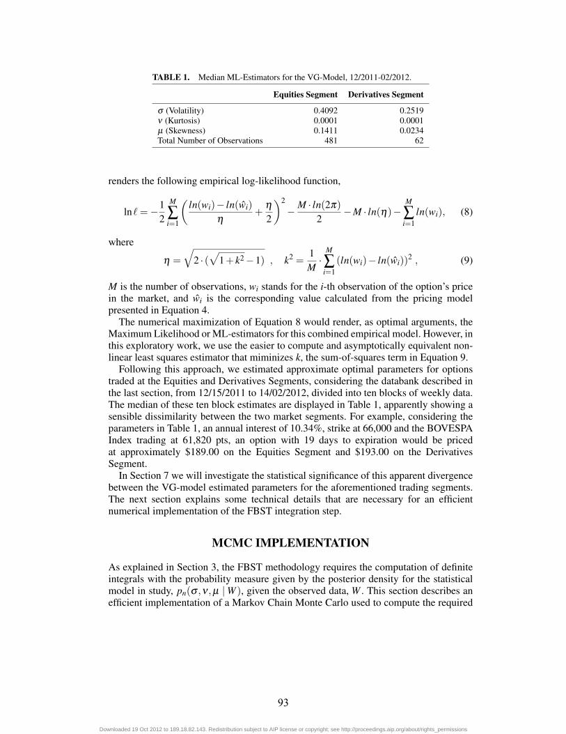
TABLE 1. Median ML-Estimators for the VG-Model, 12/2011-02/2012.

Equities Segment Derivatives Segment

σ (Volatility) 0.4092 0.2519ν (Kurtosis) 0.0001 0.0001μ (Skewness) 0.1411 0.0234Total Number of Observations 481 62

renders the following empirical log-likelihood function,

ln�=−12

M

∑i=1

(ln(wi)− ln(wi)

η+

η2

)2

−M · ln(2π)2

−M · ln(η)−M

∑i=1

ln(wi), (8)

where

η =

√2 · (

√1+ k2−1) , k2 =

1M·

M

∑i=1

(ln(wi)− ln(wi))2 , (9)

M is the number of observations, wi stands for the i-th observation of the option’s pricein the market, and wi is the corresponding value calculated from the pricing modelpresented in Equation 4.

The numerical maximization of Equation 8 would render, as optimal arguments, theMaximum Likelihood or ML-estimators for this combined empirical model. However, inthis exploratory work, we use the easier to compute and asymptotically equivalent non-linear least squares estimator that miminizes k, the sum-of-squares term in Equation 9.

Following this approach, we estimated approximate optimal parameters for optionstraded at the Equities and Derivatives Segments, considering the databank described inthe last section, from 12/15/2011 to 14/02/2012, divided into ten blocks of weekly data.The median of these ten block estimates are displayed in Table 1, apparently showing asensible dissimilarity between the two market segments. For example, considering theparameters in Table 1, an annual interest of 10.34%, strike at 66,000 and the BOVESPAIndex trading at 61,820 pts, an option with 19 days to expiration would be pricedat approximately $189.00 on the Equities Segment and $193.00 on the DerivativesSegment.

In Section 7 we will investigate the statistical significance of this apparent divergencebetween the VG-model estimated parameters for the aforementioned trading segments.The next section explains some technical details that are necessary for an efficientnumerical implementation of the FBST integration step.

MCMC IMPLEMENTATION

As explained in Section 3, the FBST methodology requires the computation of definiteintegrals with the probability measure given by the posterior density for the statisticalmodel in study, pn(σ ,ν ,μ |W ), given the observed data, W . This section describes anefficient implementation of a Markov Chain Monte Carlo used to compute the required

93

Downloaded 19 Oct 2012 to 189.18.82.143. Redistribution subject to AIP license or copyright; see http://proceedings.aip.org/about/rights_permissions

integrals, see [14] for general surveys and overviews of MCMC algorithms and theirapplication in Bayesian Statistics.

The implementation of our MCMC is based in a hierarchical combination of the Gibbsand Metropolis-Hastings algorithms, used to generate a random sample, (σ ,ν ,μ)(k),k = 1 . . .m, according to the desired posterior density, see [8].

At the higher level, the MCMC uses a Gibbs sampling procedure following a cyclicchain along conditional posterior densities, that is,

σ (k+1) ∼ pn(σ |W,ν(k),μ(k)) , (10)

ν(k+1) ∼ pn(ν |W,σ (k+1),μ(k)) , (11)

μ(k+1) ∼ pn(μ |W,σ (k+1),ν(k+1)) . (12)

At each step of the Gibbs chain, one still has to sample from non-standard, althoughunivariate, statistical distributions. This task is performed by a lower level samplingmethod based on the Metropolis-Hastings algorithm. This Metropolis-Hastings proce-dure uses a dynamically adjusted Gaussian kernel, N(0,ξ ), for generating random pro-posals, followed by the standard acceptance/rejection phase.

The numerical simulations in this article had, at the higher hierarchical level, the burn-in period, spacing among realizations and sample size, pre-set at, respectively, 200,10 and 500. Fine tuning of these parameters for the very best performance in FBSTapplications, can be accomplished using the error control method presented in [21].

CONCLUSIONS AND FINAL REMARKS

In the preceding sections we defined a coherent framework for testing the non-arbitragecondition in some financial markets based on:

1. the Fundamental Theorem of Asset Pricing;2. the Variance Gamma stochastic model for price evolution of a fundamental asset

and the associated formula for pricing european options;3. a carefully defined empirical likelihood function well suited for data analysis in

financial econometrics;4. the Full Bayesian significance test methodology;5. the efficient implementation of computational algorithms; and6. a carefully assembled data bank with price series of options on the BOVESPA

Index traded at (a) the Equities segment and (b) the Derivatives Segment of theBM&FBovespa Exchange.

A direct translation of the non-arbitrage hypothesis presented in section 3 requiresthe optimization of a six-parameter model under a three dimensional vector constraint,followed by a six-dimensional integration operation. In this exploratory work, we willtest a pair of much simpler hypotheses, namely, the point hypothesis stating that: Hab:the “true” parameters for the price model in segment (a) are equal to the maximumlikelihood estimates obtained in segment (b), and vice-versa, namely, the hypothesis

94

Downloaded 19 Oct 2012 to 189.18.82.143. Redistribution subject to AIP license or copyright; see http://proceedings.aip.org/about/rights_permissions

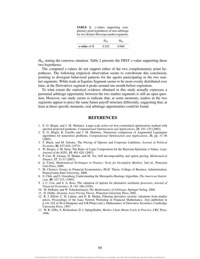
TABLE 2. e-values supporting com-plentary point hypotheses of non-arbitragefor two distinct Ibovespa market segments.

Hab Hba

e-value of H 0.242 0.066

Hba stating the converse situation. Table 2 presents the FBST e-value supporting thesetwo hypotheses.

The computed e-values do not support either of the two complementary point hy-potheses. The following empirical observation seems to corroborate this conclusion,pointing to divergent behavioral patterns for the agents participating in the two mar-ket segments: While trade at Equities Segment seems to be more evenly distributed overtime, at the Derivatives segment it peaks around one month before expiration.

To what extent the statistical evidence obtained in this study actually expresses aperennial arbitrage opportunity between the two market segments is still an open ques-tion. However, our study seems to indicate that, at some moments, traders in the twosegments appear to price the same future payoff structure differently, suggesting that, atleast at these specific moments, real arbitrage opportunities could be found.

REFERENCES

1. E. G. Birgin, and J. M. Martinez, Large-scale active-set box-constrained optimization method withspectral projected gradients, Computational Optimization and Applications, 23, 101–125 (2002).

2. E. G. Birgin, R. Castillo and J. M. Martinez, Numerical comparison of Augmented Lagrangianalgorithms for nonconvex problems, Computational Optimization and Applications, 31, pp. 31–56(2005).

3. F. Black, and M. Scholes, The Pricing of Options and Corporate Liabilities, Journal of PoliticalEconomy, 81, 637-654, (1973).

4. W. Borges, J. M. Stern, The Rules of Logic Composition for the Bayesian Epistemic e-Values. LogicJournal of the IGPL, 15, 401-420, (2007).

5. P. Carr, H. Geman, D. Madan, and M. Yor, Self decomposability and option pricing, MathematicalFinance, 17, 31-57 (2007).

6. A. Cerný, Mathematical Techniques in Finance: Tools for Incomplete Markets, 2nd ed., PrincetonUniv.Press, 2009.

7. M. Chernov, Essays in Financial Econometrics, Ph.D. Thesis, College of Business Administration,Pennsylvania State University, 2000.

8. S. Chib, and E. Greenberg, Understanding the Metropolis-Hastings Algorithm, The American Statisti-cian, 49, 327-333, (1995).

9. J. C. Cox, and S. A. Ross, The valuation of options for alternative stochastic processes, Journal ofFinancial Economics, 3, 145–166 (1976).

10. M. Delbaen, and W. Schachermayer, The Mathematics of Arbitrage, Springer Verlag, 2006.11. D. Duffie, Dynamic Asset Pricing Theory, Princeton University Press, 2001.12. R. J. Elliott, C. H. Lahaie, and D. B. Madan, Filtering derivative security valuations from market

prices, Proceedings of the Isaac Newton Workshop in Financial Mathematics. Also published inp.141-162 of M.A.Dempster and S.R.Pliska (eds.), Mathematics of Derivative Securities, CambridgeUniversity Press, 1997.

13. W. R. Gilks, S. Richardson, D. J. Spiegelhalter, Markov Chain Monte Carlo in Practice, CRC Press,1996.

95

Downloaded 19 Oct 2012 to 189.18.82.143. Redistribution subject to AIP license or copyright; see http://proceedings.aip.org/about/rights_permissions

14. A. Gelman, J. B. Carlin, H. S. Stern, and D. B. Rubin, Bayesian Data Analysis, Chapman & Hall,1998.

15. M. Harrison, and D. M. Kreps, Martingales and Arbitrage in Multiperiod Securities Market, Journalof Economic Theory, 20, 381–408, (1979).

16. M. Harrison, and S. Pliska, Martingales and Stochastic Integrals in the Theory of Continuous Trading,Stochastic Processes and Their Applications, 11, 215–260 (1981).

17. B. Ingrao, and G.Israel, The Invisible Hand: Economic Equilibrium in the History of Science, MITPress, 1990.

18. E. Jacquier, and R. A. Jarrow, Model Error in Contingent ClaimModels: Dynamic Evaluation, CiranoWorking Paper 96s-12, 1996. To appear in Journal of Econometrics.

19. E. Jacquier, and R. A. Jarrow, Bayesian Analysis of Contingent Claim Model Error, Journal ofEconometrics, 94, 145-180, (2000).

20. Jacquier, E., N.G. Polson and P.E. Rossi, Bayesian Analysis of Stochastic Volatility Models (withdiscussion): Journal of Business and Economic Statistics, 12, 371-417, (1994).

21. M. Lauretto, C. A. B. Pereira, J. M. Stern, S. Zacks, Full Bayesian Significance Test Applied toMultivariate Normal Structure Models, Brazilian Journal of Probability and Statistics, 17, 147–168,(2003).

22. D. Madan, P. Carr, and E. Chang, The Variance Gamma Process and Option Pricing, EuropeanFinance Review, 2, 79–105 (1998).

23. D. Madan, and F. Milne, Option Pricing with VG Martingale Components, Mathematical Finance,01, 39–55 (1991).

24. D. Madan, and E. Seneta, The variance gamma (V.G.) model for share market returns, Journal ofBusiness, 63, 511–524 (1990).

25. M. R. Madruga, C. A. B. Pereira, and J. M. STERN, Bayesian Evidence Test for Precise Hypotheses,Journal of Statistical Planning and Inference, 111, 185-198 (2003).

26. R. C. Merton, The Theory of Rational Option Pricing, The Bell Journal of Economics and Manage-ment Science, 04, 141-183, (1973).

27. C. A. B. Pereira and J. M. Stern, Evidence and Credibility: Full Bayesian Significance Test for PreciseHypotheses, Entropy, 01, 99-110 (1999).

28. C. A. B. Pereira, J. M. Stern, Special Characterizations of Standard Discrete Models. REVSTATStatistical Journal, 6, 199–230, (2008).

29. C. A. B. Pereira, J. M. Stern, S. Wechsler, Can a Significance Test be Genuinely Bayesian? BayesianAnalysis, 3, 79–100, (2008).

30. M. Rubinstein, Implied Binomial Trees, The Journal of Finance, 49, 771-818 (1994).31. A. N. Shiryaev, Essentials of Stochastic Finance: Facts, Models, Theory, World Scientific Publishing

Company, 1999.32. J. M. Stern, Constructive Verification, Empirical Induction, and Falibilist Deduction: A Threefold

Contrast, Information, 02, 635-650 (2011).33. A. V. Skorokhod, Studies in the Theory Random Processes, Addison-Wesley, 1967.

96

Downloaded 19 Oct 2012 to 189.18.82.143. Redistribution subject to AIP license or copyright; see http://proceedings.aip.org/about/rights_permissions