Noise & Uncertainty ASTR 3010 Lecture 7 Chapter 2.

Noise & Uncertainty

ASTR 3010

Lecture 7

Chapter 2

Accuracy & Precision

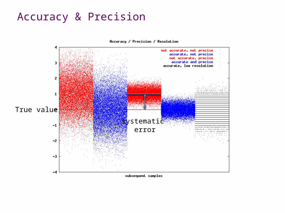
Accuracy & Precision

True value

systematic error

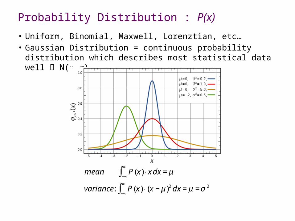
Probability Distribution : P(x)

• Uniform, Binomial, Maxwell, Lorenztian, etc…• Gaussian Distribution = continuous probability distribution which describes

most statistical data well N(,)

€

mean: P(x)⋅ x dx = μ−∞

∞

∫variance : P(x)⋅ (x − μ)2 dx = μ

−∞

∞

∫ =σ 2

Binomial Distribution

• Two outcomes : ‘success’ or ‘failure’probability of x successes in n trials with the probability of a success at each trial

being ρ

Normalized…

mean

when

€

P x;n,ρ( ) =n!

x!(n − x)!ρ x (1− ρ )n−x

€

P x;n,ρ( )x=0

n

∑ =1

€

P x;n,ρ( )x=0

n

∑ ⋅ x =K = np

€

n →∞ ⇒ Normaldistribution

n →∞ and np = const ⇒ Poissonian distribution

Gaussian Distribution

€

G(x) =1

2πσ 2exp −

x − μ( )2

2σ 2

⎡

⎣ ⎢ ⎢

⎤

⎦ ⎥ ⎥

Uncertainty of measurement expressed in terms of σ

Gaussian Distribution : FWHM

+t

€

G(μ + t) =1

2G(μ) → t =1.177σ

€

2.355σ

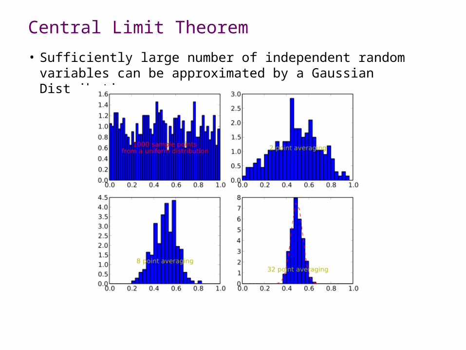
Central Limit Theorem

• Sufficiently large number of independent random variables can be approximated by a Gaussian Distribution.

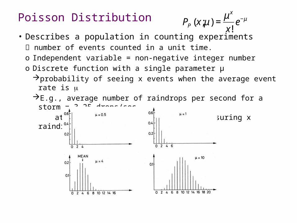
Poisson Distribution

• Describes a population in counting experiments number of events counted in a unit time.o Independent variable = non-negative integer numbero Discrete function with a single parameter μprobability of seeing x events when the average event rate is E.g., average number of raindrops per second for a storm = 3.25 drops/sec at time of t, the probability of measuring x raindrops = P(x, 3.25)

€

PP (x;μ) =μ x

x!e−μ

Poisson distribution

Mean and Variance

€

x = xx=0

∞

∑ PP (x;μ) = xμ x

x!e−μ

⎛

⎝ ⎜

⎞

⎠ ⎟

x=0

∞

∑

=K

= μ

(x − μ)2 =K

= x 2 − μ 2

=K

= μ €

μx

x!x=0

∞

∑ = eμuse

Signal to Noise Ratio

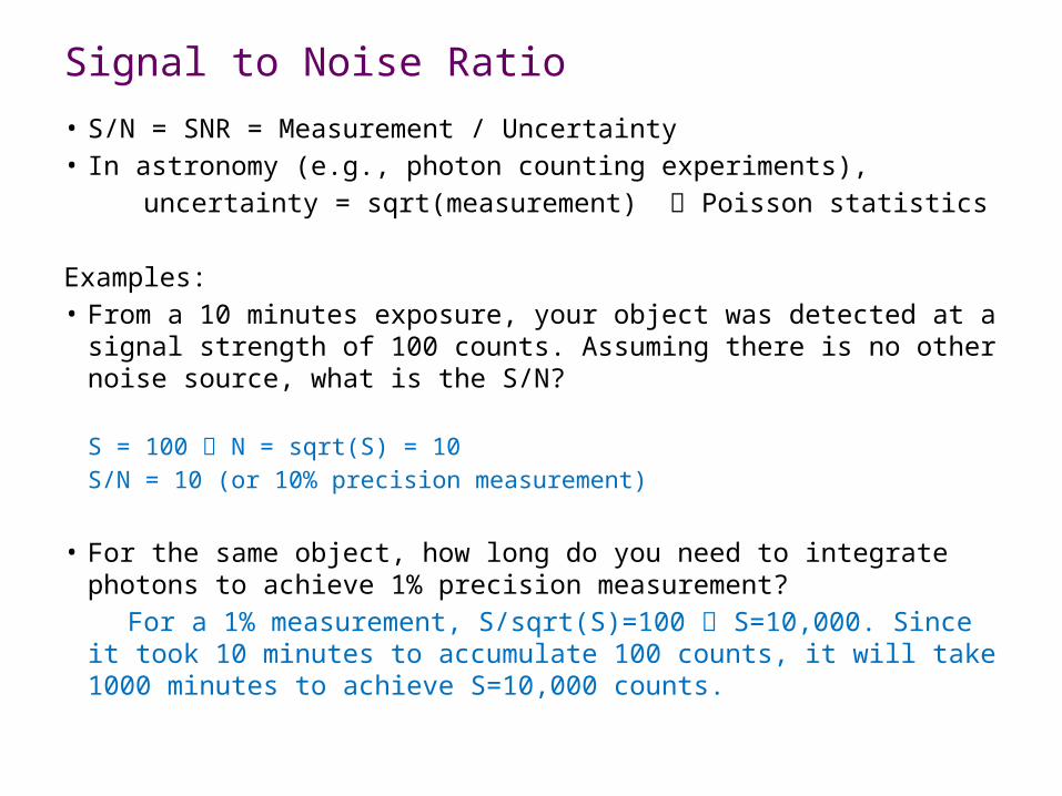
• S/N = SNR = Measurement / Uncertainty• In astronomy (e.g., photon counting experiments), uncertainty = sqrt(measurement) Poisson statistics

Examples:• From a 10 minutes exposure, your object was detected at a signal strength

of 100 counts. Assuming there is no other noise source, what is the S/N?

S = 100 N = sqrt(S) = 10S/N = 10 (or 10% precision measurement)

• For the same object, how long do you need to integrate photons to achieve 1% precision measurement?

For a 1% measurement, S/sqrt(S)=100 S=10,000. Since it took 10 minutes to accumulate 100 counts, it will take 1000 minutes to achieve S=10,000 counts.

Weighted Mean

• Suppose there are three different measurements for the distance to the center of our Galaxy; 8.0±0.3, 7.8±0.7, and 8.25±0.20 kpc. What is the best combined estimate of the distance and its uncertainty?

wi = (11.1, 2.0, 25.0)

xc = … = 8.15 kpc

c= 0.16 kpc

So the best estimate is 8.15±0.16 kpc.

2

2

1 22

1

11

c

ii

n

ii

c

n

iiic wwxx

Propagation of Uncertainty

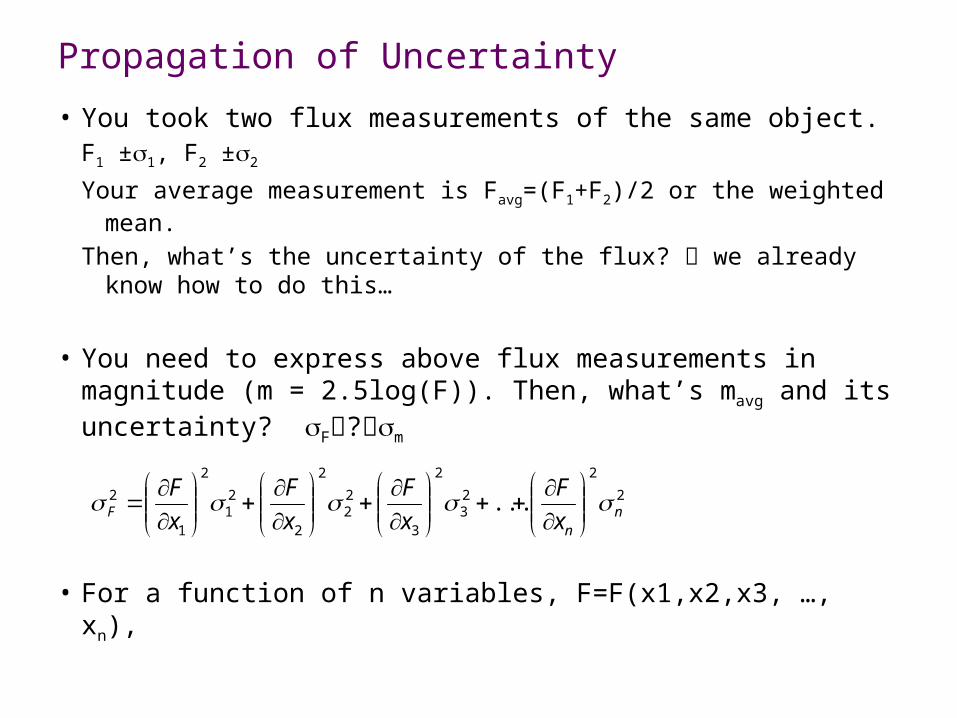
• You took two flux measurements of the same object. F1 ±1, F2 ±2

Your average measurement is Favg=(F1+F2)/2 or the weighted mean.

Then, what’s the uncertainty of the flux? we already know how to do this…

• You need to express above flux measurements in magnitude (m = 2.5log(F)). Then, what’s mavg and its uncertainty? F?m

• For a function of n variables, F=F(x1,x2,x3, …, xn),

2

2

23

2

3

22

2

2

21

2

1

2 ... nn

F x

F

x

F

x

F

x

F

Examples

1. S=1/2bh, b=5.0±0.1 cm and h=10.0±0.3 cm. What is the uncertainty of S?

S

h

b

Examples

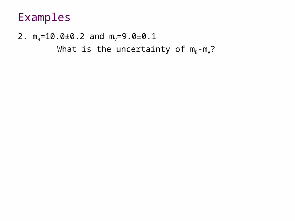
2. mB=10.0±0.2 and mV=9.0±0.1

What is the uncertainty of mB-mV?

Examples

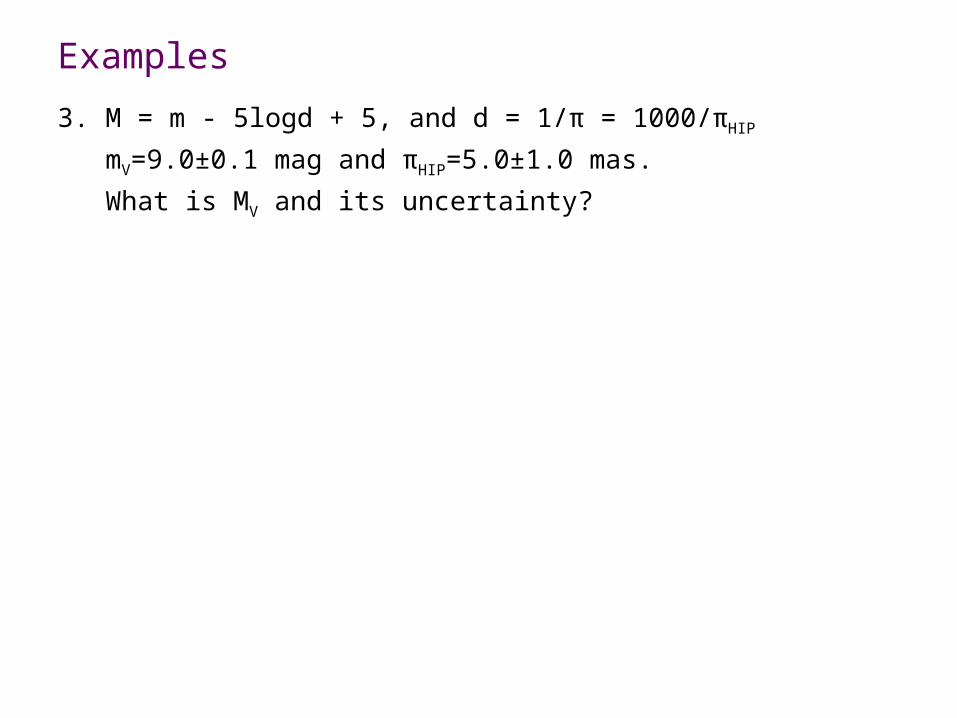
3. M = m - 5logd + 5, and d = 1/π = 1000/πHIP

mV=9.0±0.1 mag and πHIP=5.0±1.0 mas.

What is MV and its uncertainty?

In summary…

Important Concepts• Accuracy vs. precision• Probability distributions and

confidence levels• Central Limit Theorem• Propagation of Errors• Weighted means

Important Terms• Gaussian distribution• Poisson distribution

Chapter/sections covered in this lecture : 2